The Lake Okeechobee Water Quality Model (LOWQM) · EXECUTIVE SUMMARY The Lake Okeechobee Water...

S O U T H F L O R I D A W A T E R M A N A G E M E N T D I S T R I C T

The Lake Okeechobee Water Quality Model (LOWQM): Calibration/Validation Update 2012

WR-2013-002

R. Thomas James Lead Environmental Scientist Lake and River Ecosystems Section

Applied Sciences Bureau Water Resources Department

11/12/2013

i

TABLE OF CONTENTS Figures ............................................................................................................................................. ii Tables ............................................................................................................................................. iii Executive Summary ........................................................................................................................ 4

Introduction ..................................................................................................................................... 5

Model Description ........................................................................................................................... 5

Site Description ............................................................................................................................... 6

Monitoring Data .............................................................................................................................. 8

Hydrology and Nutrient Loads ................................................................................................. 8

Meteorology and Water Volume .............................................................................................. 8

Water Quality ............................................................................................................................ 8

Phytoplankton Density .............................................................................................................. 9

Sediment Quality .................................................................................................................... 10

Model Calibration and Validation ................................................................................................. 10

Water Budget .......................................................................................................................... 11

Resuspension and Settling ...................................................................................................... 11

Observed Data and Calibration and Validation Techniques ................................................... 13

Results ........................................................................................................................................... 14

Water Column Calibration and Validation ............................................................................. 14

Comparison of Original and Current LOWQM Calibration ................................................... 23

Sediment Calibration and Validation ...................................................................................... 24

Comparison to Measured Rates .............................................................................................. 24

Discussion ..................................................................................................................................... 26

Phosphorus .............................................................................................................................. 27

Nitrogen .................................................................................................................................. 27

Silica ....................................................................................................................................... 28

Algae ....................................................................................................................................... 28

Sediments and Sediment Water Interactions .......................................................................... 29

Suggested Model Improvements ................................................................................................... 29

Conclusions ................................................................................................................................... 29

Literature Cited .............................................................................................................................. 30

Appendix A. Phosphorus-Related Parameters................................................................................ 34

Appendix B. Original and New Calibration of Phytoplankton Parameters .................................... 36

Appendix C. Additional Original and New Calibration Parameters .............................................. 38

ii

FIGURES Figure 1. Diagram of the enhanced LOWQM. ............................................................................... 6

Figure 2. Map of Lake Okeechobee showing monitoring locations for inflows/outflows in-lake water quality (WQ), meteorology, and phytoplankton. ................................................................................................................. 7

Figure 3. (A) Sediment resuspension rate and (B) monthly averaged synthetic observations and simulated ISS ..................................................................................... 12

Figure 4. Simulated and monthly average observed values for (A) TP and (B) DIP.................... 18

Figure 5. Simulated and monthly average observed values for (A) TN and B) DIN.................... 19

Figure 6. Simulated and monthly average observed values for (A) NH4, (B) NOx and (C) DSI. ......................................................................................................................... 20

Figure 7. Simulated and monthly averaged observed values for (A) CHLA and (B) total algal C. ............................................................................................................ 21

Figure 8. Simulated and monthly averaged observed values for (A) cyanobacteria, (B) diatoms and (C) green algae. ................................................................................... 22

iii

TABLES Table 1. Regression equations and coefficients of determination (R2) for three

relationships to ISS using log transformed observed data from the eight station network L001-L008 from 1972 to present.......................................................... 9

Table 2. Calibration period (1997–2012) numerics for water column observed and simulated measurements. (Note: N – number of comparisons, O – observed, S – simulated, sd – standard deviation. Bold indicates an acceptable statistical comparison.) ................................................................................................. 15

Table 3. Validation period (1983–1996) numerics for water column observed and predicted variables. (Note: O – observed, S – simulated, sd – standard deviation. Bold indicates an acceptable statistical comparison.) ................................. 16

Table 4. Counts of the four numerical comparisons that were better, worse or did not change (by 5%) in contrasting the updated calibration over the original calibration. ...................................................................................................... 23

Table 5. Observed (from raw data of Fisher et al. 2001, Olila et al. 1995, Reddy 1991 and BEM and University of Florida 2007) and predicted mean and standard deviations for sediments of Lake Okeechobee mg l-1 for the top 6 cm of sediment. (Note: O –observed, S –simulated, sd – standard deviation. Bold indicates the result is within one standard deviation of the observed mean. Bold underline indicates the result is within two standard deviations of the observed mean.) ................................................................................................. 25

Table 6. Measured and simulated algal growth and N flux rates (mg m-2 d-1) ........................... 26

4

EXECUTIVE SUMMARY The Lake Okeechobee Water Quality Model (LOWQM) was developed to evaluate the

management of external nutrient load reductions on in-lake and in-sediment nutrient concentrations over a multi-decadal scale. This moderately complex model (Figure 1) was originally calibrated/validated to hydro-meteorological and monitoring data from 1982 to 2000. The model has been used to predict the effects of upstream hydrologic and nutrient management scenarios on downstream nutrient loads to estuaries and effects of sediment management options on in-lake nutrient conditions.

A series of extreme hydro-meteorological events occurred from 2005 to 2008 that were outside the range of observations in the original LOWQM calibration. Three hurricanes, Frances (September 4, 2004), Jeanne (September 26, 2004) and Wilma (October 25, 2005) directly affected the lake resulting in major sediment resuspension and increased water levels. This period of disturbance was followed by a major drought from 2006 to 2007. These extreme weather events resulted in major changes of the light environment, nutrients and phytoplankton in the lake.

The purpose of this current effort is to update the LOWQM calibration/validation to lengthen the simulation period and to include these extreme hydro-meteorologic events. Including these events increases the confidence that the LOWQM can accurately predict the outcome of future load reduction scenarios.

Specifically, the LOWQM was expanded to include the period January 2001 to April 2012. Inflow, discharge, nutrient loads, rainfall, and evaporation data from this period were added. Sediment resuspension, modeled as an external forcing function, was also revised and expanded. The period of January 1997 to April 2012 was used to recalibrate the model. The recalibration consisted of systematically changing model parameters within reasonable ranges; running the model using the timeline of nutrient loads, sediment resuspension, flows and weather for 1997 to 2012; and comparing model results to observed data for this period using four numerical comparisons. This tuning of model parameters was carried out to find the best numeric comparisons for nutrients and phytoplankton. Once completed, a validation run of the model was carried out for the January 1982 to December 1996 period. To do this the tuned parameters were unchanged, the timeline of nutrient loads, sediment resuspension, flows and weather for the 1982 to 1996 period were input to the model, and the model results were compared to observed data for this period.

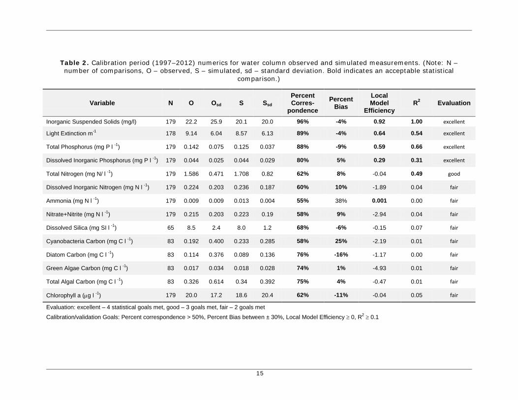
A number of input parameters were changed to allow model results to more closely match observed measurements from 1997 to 2012 (see Appendices A, B and C). The four numerical comparisons used between model predictions and observed measurements were percent bias, percent correspondence, local model efficiency, and R2. Each one of these comparisons tests the model results differently. Percent bias test the amount of under or over prediction by the model. Percent correspondence determines if the model is within the range of observed data variation. Local model efficiency determines if the model results follows observed trends and stays within the range of the observed data over time. R2 determines how well the model tracks the observed data over time. Model calibration was excellent (four out of four statistical goals met) for inorganic suspended solids, light extinction, total phosphorus (TP) and dissolved inorganic phosphorus (DIP), good (three out of four met) for total nitrogen (TN), and fair (two out of four met) for all others.

Model validation was excellent for inorganic suspended solids, light extinction, TP, DIP, TN, cyanobacteria, and chlorophyll a (CHLA), good for dissolved inorganic nitrogen (DIN), nitrate+nitrite nitrogen (NOx), green algae, and total algal carbon (C), and fair for all others. Model sediment estimates for various nutrients were compared to field measurements taken at

5

three separate years from 171 locations in the lake. Model estimates were within the one standard deviation of the mean of measurements at each time point, with the exception of one year of particulate organic phosphorus (P) and two years of DIN (that were within two standard deviations of the mean). An additional validation was comparing various nutrient uptake rates measured at given points in time and space on the lake to the median 25th and 75th percentiles of these rates simulated by the model. With the exception of ammonia (NH4) uptake, the model simulation encompassed the observed measured values. The updated calibration was as good (within 5% of the numeric criteria) or better than the original calibration for 49 of the 56 numeric comparisons for the calibration period (88%) and 44 of 56 numeric comparisons for the validation period (78%).

A number of model enhancements are suggested to improve nitrogen (N) and phytoplankton performance. Despite this varied performance of model constituents, overall the model is calibrated and validated to a wider range of conditions that will provide more reliable results for future management scenarios. Sensitivity and uncertainty analyses are recommended for these future simulations because of the unequal calibration success among modeled components.

INTRODUCTION Lake Okeechobee has experienced decades of excessive external phosphorus (P) loads

(Havens et al. 1996, Havens and James 2005). As the lake has become more culturally eutrophic, increases in TP, algal blooms (determined from events where CHLA concentrations exceed 40 micrograms per liter [µg l-1]), and increased cyanobacteria dominance occurred through the 1990s (Havens et al. 1996).

Numerous management programs to reduce external TP loads to the lake have been implemented since the 1970s. Despite reduced loads to the lake, the average annual P concentration in the lake has remained well above the Total Maximum Daily Load (TMDL) goal of 0.040 milligrams (mg) P per liter (l-1) (FDEP 2001). The explanation for this lack of response is that sediments, which contain a large pool of P—estimated at 28,700 metric tons in the top 10 centimeters (cm) (Reddy et al. 1995)—buffer the in-lake TP. Havens and James (2005) demonstrated this from annual nutrient budgets, which showed a decline of that net settling of P to the sediments over time as nutrient loads to the lake declined.

The LOWQM (Figure 1) was developed to provide an understanding of internal nutrient cycling within the lake—specifically TP—and to assess lake-wide responses to various management alternatives. This model has been used to support a number of programs and projects including the Lake Okeechobee TMDL (FDEP 2001), the Comprehensive Everglades Restoration Program (CERP) (RECOVER 2007), and the Lake Okeechobee Sediment Feasibility Study (Blasland Bouck and Lee Inc. 2001, James and Pollman 2011).

MODEL DESCRIPTION The LOWQM is a deterministic, mass balance model based on an enhanced version of

EUTRO5, the eutrophication submodel of the Water Quality Analysis Simulation Program, Version 5 (WASP5) (Ambrose et al. 1993a, 1993b). The model partitions the lake into three homogenous compartments: water column, oxic surface sediment and anoxic deeper sediment. It simulates the N, P, Silica (SI) and oxygen cycles, as well as phytoplankton dynamics (Figure 1) (James et al. 2005). The model uses a 0.08 day time step, and it prints out values on a daily basis.

6

Figure 1. Diagram of the enhanced LOWQM.

The LOWQM was enhanced based on recommendations by James and Bierman (1995), including the addition of surface sediment layers and sediment processes that affect nutrient availability in the water column; sediment resuspension; and changing water depth and interfacial area between sediment and water column as the lake volume changes. These improvements were documented in James et al. (1997) and the equations that involve resuspended solids and their impact on light and DIP are defined in James et al. (2005).

Further enhancements were made by James et al. (2005) to improve the model’s ability to predict decadal-scale response to external nutrient load reductions. These included four organic P (OP) classes based on degradability and solubility: (labile, moderately labile and non-degradable particulate P and dissolved P); three algal groups to represent the major algal classes in the lake (N-fixing cyanobacteria, diatoms and green algae); and SI dynamics to simulate a diatom group (Figure 1). This current version of LOWQM includes over 100 parameters that can be adjusted to calibrate the model to measured nutrient, chlorophyll, biomass and fluxes (Appendices A, B and C; also see James et al. 2005).

SITE DESCRIPTION Lake Okeechobee is a large (1,730 square kilometers) shallow (mean depth 2.7 meters [m])

lake in the south central region of the Florida Peninsula (Figure 2). It is important for native wildlife, sport and recreation, flood control and water supply for the surrounding area as well as the Everglades and the Caloosahatchee and St. Lucie estuaries. The lake has been studied extensively (Aumen and Wetzel 1995) and has been monitored for hydrology and water quality on a routine basis since 1972 (James et al. 1995a, 1995b, Zhang and Sharfstein 2013).

7

Figure 2. Map of Lake Okeechobee showing monitoring locations for inflows/outflows in-lake water quality (WQ), meteorology, and phytoplankton.

8

MONITORING DATA Lake Okeechobee water quality and flow data have been measured at 33 inflow/outflow

locations on a monthly to biweekly basis from 1973 to present (Figure 2). Water quality samples have been collected for the same time period at nine in-lake locations. In addition, phytoplankton have been measured at four stations between 1988 and 1992 (Cichra et al. 1995). After 1993, two of these locations were sampled and additional samples were taken from two alternate locations (Beaver et al. 2013). These data were used to develop and calibrate the LOWQM as described by James et al. (2005). The hydrology and water quality data are available from the South Florida Water Management District’s (District’s) DBHYDRO database (SFWMD 2012), the phytoplankton and sediment data are available from the District’s Ecological Data Management System (EDMS) (SFWMD 2011b).

HYDROLOGY AND NUTRIENT LOADS The inflow/outflow and associated water quality measurements are used to calculate nutrient

loads to and from Lake Okeechobee. These are reported in the Lake Okeechobee Watershed Protection Plan (Figure 2) (Zhang and Sharfstein 2013) and the Lake Okeechobee Operating Permit Annual Report (James and Sharfstein 2013). Nutrient and water budgets are calculated from these data and summed by month for inflows and outflows (James et al. 1995a). Flow and flow-weighted nutrient concentrations (calculated from flow and load) are boundary conditions in the input data set for the model.

METEOROLOGY AND WATER VOLUME Rainfall, evaporation, solar radiation and water temperature are measured at a network of

stations throughout the lake area (Figure 2) and also are calculated using next generation radar (NEXRAD) and satellite imagery (SFWMD 2011a). These data are averaged by month and used as forcing functions of the LOWQM.

Lake volume is estimated from daily measured stage data (SFWMD 2012; DBKEY 15611) using a stage storage relationship (USACE 1978). These daily volumes are used to set day 0 volume for the model and are used to compare observed and predicted volumes over time.

WATER QUALITY In-lake water quality measurements were averaged by month for use in comparisons for

model calibration and validation. Rigorous quality assurance and quality control procedures (SFWMD 1999) were in place after 1982; therefore, only data after 1982 were used in this calibration and validation process. Monthly means and standard deviations were calculated for TP and DIP, NH4, NOX, and TN (total Kjeldahl nitrogen + NOX), light extinction (Ke as 1.9/Secchi Disk depth), CHLA, and inorganic suspended solids (ISS). Dissolved silica (DSI) was also included, but it was measured and averaged quarterly.

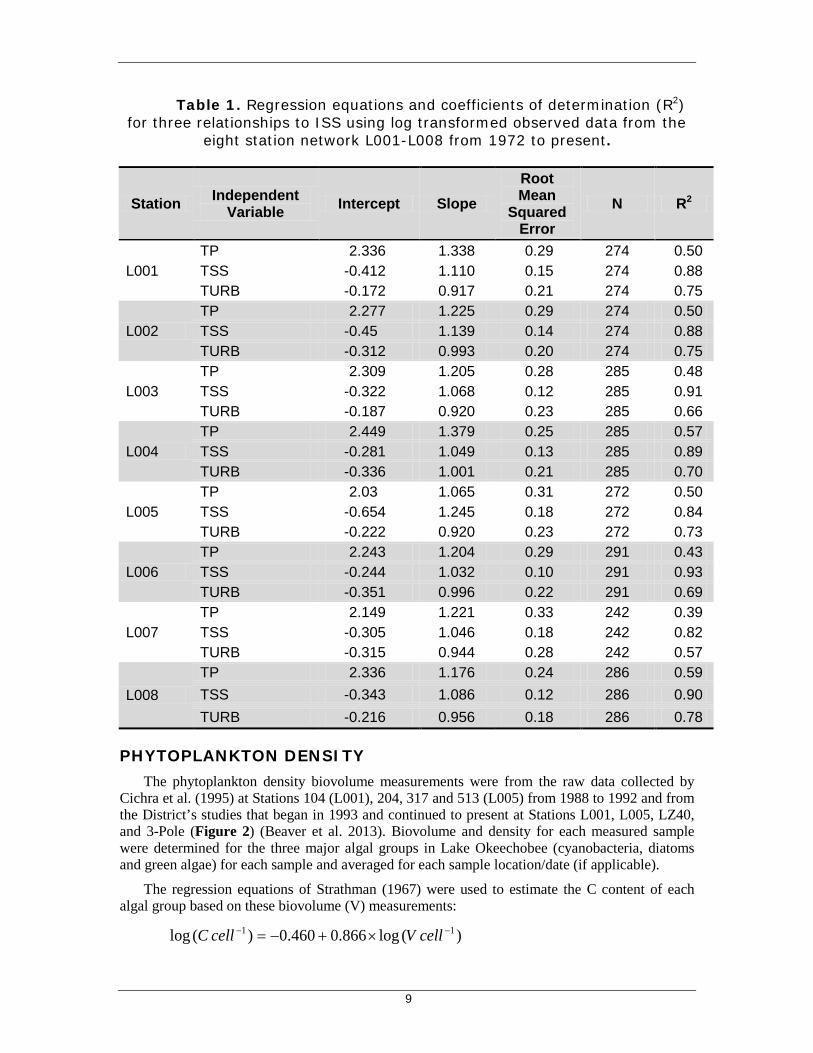
ISS were a critical component to estimate sediment water interactions. ISS was measured in the lake water column from 1974 to 1977 and 1990 to present, total suspended solids (TSS) from 1974 to 1977 and 1981 to present, turbidity (TURB) 1973 to present and TP from 1973 to present. Missing ISS data were estimated for each sampling location using log-log relationships between ISS and TSS, ISS and TURB, and ISS and TP, in that order respectively (Table 1). This filled in time series of synthetic raw data set of ISS (RISS) was used to develop the resuspension forcing function as described in the Resuspension and Settling section (below).

9

Table 1. Regression equations and coefficients of determination (R2) for three relationships to ISS using log transformed observed data from the

eight station network L001-L008 from 1972 to present.

Station Independent Variable Intercept Slope

Root Mean

Squared Error

N R2

L001 TP 2.336 1.338 0.29 274 0.50 TSS -0.412 1.110 0.15 274 0.88 TURB -0.172 0.917 0.21 274 0.75

L002 TP 2.277 1.225 0.29 274 0.50 TSS -0.45 1.139 0.14 274 0.88 TURB -0.312 0.993 0.20 274 0.75

L003 TP 2.309 1.205 0.28 285 0.48 TSS -0.322 1.068 0.12 285 0.91 TURB -0.187 0.920 0.23 285 0.66

L004 TP 2.449 1.379 0.25 285 0.57 TSS -0.281 1.049 0.13 285 0.89 TURB -0.336 1.001 0.21 285 0.70

L005 TP 2.03 1.065 0.31 272 0.50 TSS -0.654 1.245 0.18 272 0.84 TURB -0.222 0.920 0.23 272 0.73

L006 TP 2.243 1.204 0.29 291 0.43 TSS -0.244 1.032 0.10 291 0.93 TURB -0.351 0.996 0.22 291 0.69

L007 TP 2.149 1.221 0.33 242 0.39 TSS -0.305 1.046 0.18 242 0.82 TURB -0.315 0.944 0.28 242 0.57

L008 TP 2.336 1.176 0.24 286 0.59 TSS -0.343 1.086 0.12 286 0.90 TURB -0.216 0.956 0.18 286 0.78

PHYTOPLANKTON DENSITY The phytoplankton density biovolume measurements were from the raw data collected by

Cichra et al. (1995) at Stations 104 (L001), 204, 317 and 513 (L005) from 1988 to 1992 and from the District’s studies that began in 1993 and continued to present at Stations L001, L005, LZ40, and 3-Pole (Figure 2) (Beaver et al. 2013). Biovolume and density for each measured sample were determined for the three major algal groups in Lake Okeechobee (cyanobacteria, diatoms and green algae) for each sample and averaged for each sample location/date (if applicable).

The regression equations of Strathman (1967) were used to estimate the C content of each algal group based on these biovolume (V) measurements:

)(log866.0460.0)(log 11 −− ×+−= cellVcellC

10

for both green algae and cyanobacteria and

)(log758.0422.0)(log 11 −− ×+−= cellVcellC

for diatoms. The C per cell estimates were multiplied by the cell densities to determine mg C l-1 for each phytoplankton group. The monthly lake means and standard deviations were calculated from the appropriate samples for each group. These values were used to compare to model results using the four goodness-of-fit criteria.

SEDIMENT QUALITY Sediment nutrient and density data (e.g., mg P per kilogram [kg-1] sediment and kilogram

(kg) l-1 sediment for density) were measured by Reddy (1991), Fisher et al. (2001), and BEM and University of Florida (2007) in the top 10 cm of samples from 171 locations. Particulate inorganic P (IP) was extracted from each core using potassium chloride (KCL) (solution concentration of 1 mole per liter [1-M]), sodium hydroxide (NaOH) (1-M) or sodium bicarbonate (NaHCO3) (1-M) and hydrogen chloride (HCL) (1-M) in that order. The extractions were analyzed for IP and summed. These measurements (reported in mg kg-1 sediment) were multiplied by the given sediment sample’s dry bulk density (kg l-1 sediment) to transform the nutrient values to mg l-1 sediment (the units used in the model). DIP samples measured from the interstitial water were multiplied by the amount of water in the sediment to obtain total amount in a given volume of sediment, and then were divided by the total volume of sediment to obtain values to mg l-1 of sediment.

TP was determined from whole sediment samples extracted with a nitric acid/hyper-chlorate digest (Reddy 1991, Fisher et al. 2001). The difference between the TP and summed inorganic P was considered particulate organic P (POP). Along with DIP and OP, these measurements were averaged over the 171 locations to obtain average sediment nutrient concentrations and to determine the variance of each measurement (standard deviation). A similar methodology was employed to determine particulate inorganic and organic N and DIN and dissolved organic nitrogen (DON).

Nutrient fluxes measured from sediment cores in the lake (Moore et al. 1998, Fisher et al. 2005) were used to further validate model results. The observed lake mean and standard deviation of these measurements were compared to the model predictions for the appropriate years (1989 and 1998). Measurements of N uptake, nitrogen gas (N2) fixation, and algal productivity were determined for one day on Lake Okeechobee (Gu et al. 1997). In addition, various measurements of denitrification were made by Messer and Brezonik (1983). These values were used to further validate the LOWQM simulation.

MODEL CALIBRATION AND VALIDATION The LOWQM was applied to Lake Okeechobee for two periods (1) January 1997 to April

2012 for calibration and (2) January 1983 to December 1996 for validation. Comparisons between model predictions and observed data were made on a monthly basis. Observed measurements were averaged and standard deviations calculated by month for each year. Simulated output values were selected by using only values that represent the dates when observed data were taken. The selected simulated data were then averaged by month for each year and compared to the observed data using four separate goodness-of-fit numerics described in the Observed Data and Calibration and Validation Techniques section (below).

11

WATER BUDGET The model calculated Lake Okeechobee’s water budget from time series of inflows, outflows,

evaporation and rainfall. These time series were daily rates estimated from monthly averaged values. The initial volume was the appropriate day zero value (December 31, 1996 for the calibration, or December 31, 1982 for the validation) estimated from lake stage measurements (James et al. 2005). The model calculated volumes at each time step based on the previous time step volume and these time series. The initial time series of evaporation values was adjusted for each month to match model-predicted volumes to volumes for the lake estimated from lake stage measurements (James et al. 2005).

RESUSPENSION AND SETTLING The RISS data set as described in the Water Quality section (above) was reduced by

averaging together data that were sampled during the same week. This method insured each average value included samples from all regions of the lake under similar weather conditions. This averaged data set was used to develop the sediment resuspension rates.

A constant gross settling rate, VISS, (59 cm per day [d-1]) was specified for ISS in the model, based on the work of Mehta (1991). The time series of sediment resuspension, WST (Figure 3a), was developed for 1983–2012 by adjusting resuspension values until simulated ISS values closely matched the averaged RISS values (Figure 3b). The sediment resuspension rate was applied to the day of the observed measurement and all days in between the previous observed measurement and the current measurement (e.g., a stair step function). WST averaged 0.0028 cm of sediment day-1 (95% confidence interval 0.0001–0.008 cm of sediment day-1), with a maximum of 0.023 and a minimum of 0.0000 cm of sediment day-1.

The resultant resuspension of ISS simulated by the LOWQM ranged from near zero to over 80 grams per square meter per day (g m-2 d-1) (Figure 3a). Because inorganic solids represent approximately half of the solids in the lake, the estimated flux from the sediments is 0 to 160 g m-2 d-1 or 0 to 7 g m-2 per hour (h-1). Mehta (1991) measured potential erosion rates of sediment cores taken from Lake Okeechobee with a laboratory flume. Depending on the shear stress, he found hourly erosion values ranging from 1 to 576 g m-2 hr-1 of total sediment resuspension. Since LOWQM values are daily average, it is understandable that they are on the low end of the instantaneous rates measured by Mehta (1991).

All particulate nutrients and algae in sediments were resuspended using this calibrated WST time series. Although the model could calculate these fluxes from wind speed and direction data, as in James et al. (1997), these data were incomplete for the 30+ year period of the simulation and were therefore not used.

To close the sediment/water mass balance loops, a gross settling rate for organic P and N—VO (9.5 cm day-1)—was used to tune observed monthly averaged values. This VO value was constant throughout the simulation. The fraction of DON in the water column and sediment (FDON) was unchanged from the previous calibration (James et al. 2005) using a ratio of 0.002 mg DON mg-1 TN, which produce simulated TN that closely matched observed monthly averaged TN values (Appendix C). This constant fraction of DON was similar to the fraction of DON to TN measured in Lake Okeechobee sediments (Reddy 1991).

As in James et al. (2005), a surficial aerobic sediment layer and a subsurface anaerobic layer approximating the mixed layer depth was specified. Processes of decomposition, sediment oxygen uptake, and denitrification occurred in these sediments at different rates as determined by aerobic or anaerobic conditions. The surficial layer thickness was specified as one cm, consistent with measurements by Moore and Reddy (1994). An underlying anaerobic layer was set to a thickness of 5 cm. Nutrients were mixed in these layers through both diffusion and particle

12

mixing within the sediments (Appendix C: Dss, Smix respectively) and diffusion between the sediment and water column (Dsw). Sediments below 6 cm were considered permanently buried and outside the system with no communication upward. Subsurface sediments and all contents were buried out of the system at a constant rate, Vb (0.095 cm year-1)–determined from Pb210 studies of sediments in Lake Okeechobee (Brezonik and Engstrom 1998). This assumption of a 6-cm layer of sediment was based on three separate observations presented in James et al. (2005):

1. Brezonik and Engstrom (1998) found highest TP concentrations in the top 5 cm of sediment. 2. Kirby et al. (1994) found sub-millimeter laminations in mud sediments that disappeared

toward the top of the sediments suggesting that resuspension only affects the upper few cm of sediments.

3. Sediment cores taken after Hurricane Irene passed over the lake in October 1999 did not show signs of major disturbance below the first 5 cm of sediments (John White, Research Scientist, University of Florida, personal communication).

This assumption will be reconsidered in the future as the hurricane events of 2004 and 2005 did affect sediments at deeper depths (Jin et al. 2011).

Figure 3. (A) Sediment resuspension rate and (B) monthly averaged synthetic

observations and simulated ISS

0102030405060708090

Sedi

men

t res

uspe

nsio

n

mg

ISS

m-2

d-1

A

0

20

40

60

80

100

120

140

Inor

gani

c Su

spen

ded

Solid

s m

g/L

Synthetic observations Modeled

validation calibration

B

13

James et al. (2005) found that preliminary model simulations predicted dramatic declines of sediment ISS, primarily a result of the specified net burial rate, which was constrained by independent measurements of lead 210 isotope (Pb210) dating of sediment cores (Brezonik and Engstrom 1998). A review of sediment data for Lake Okeechobee (Brezonik and Engstrom 1998) and the model-computed fluxes indicate that the model was apparently missing a source of inorganic solids. James et al. (2005) assumed that settling of calcium carbonate, which is not simulated in the model but makes up 12 to 40 percent of dry sediments in the lake, was the source of the missing material. James et al. (2005) added a load of 239 g m-2 year-1 [note this is the value used in the original calibration but was misreported by James et al. (2005) as 327 m-2 year-1]. The same 239 g m-2 year-1 or 1.13 x 106 kg d-1 external load was maintained in this calibration effort (Appendix C).

OBSERVED DATA AND CALIBRATION AND VALIDATION TECHNIQUES

All initial values used for kinetic rates were based on those used by James et al. (2005) (Appendices A, B and C). These values were constrained within acceptable ranges as defined in Bowie et al. (1985), Thomann and Mueller (1987), and Ambrose et al. (1993b). Calibration was done in the order: ISS, TP, DIP, TN, DIN, NOX, NH4, DSI, CHLA, and phytoplankton C (cyanobacteria, diatom, and green algae). Parameters were systematically calibrated to the monthly averaged data based on this calibration order. The fine tuning did require some back and forth trial and error to obtain the best calibration set.

Observed and model-predicted monthly average data were compared using four goodness-of-fit measures including percent bias, R2, percent correspondence and local model efficiency (James et al. 2005). Percent bias is the average monthly difference between the simulated and observed data divided by the averaged observed data. This numeric determines if model results consistently over or under predict observed data. R2 is the amount of monthly observed variance described by the model simulation. This numeric determines how well the model follows any trends in the data. Percent correspondence (%Corr) compares the number of monthly model predictions that were within the monthly averaged 95% confidence interval (NC) to the total number of comparisons, Nt:

This numeric indicates how well the simulation stays within the range of observed data. Local model efficiency (LME) is calculated using the formula:

Where tO is the averaged observed value for a given month (denoted as t), tS is the monthly average of simulated values corresponding to the dates when the observed values were collected and Ncomp is the total number of monthly comparisons. This difference is divided by twice the standard deviation, OSDt, of the monthly observed values:

100% NN = Corr

t

c ×%

compNO

OS

LME

compN

t SDt

tt∑=

×−

−= 1 2||

1

t

N

i ttiSDt N

OOO

t∑=−

= 12)(

14

Where Oti is the mean monthly observed value from an individual station i in month t and Nt is the number of stations contributing to the samples in month t. This final numeric indicates how precise the model follows the observed data accounting for variability of the observed data.

Monthly differences are summed and then divided by Ncomp to obtain an overall average that could range from 0 to infinity. Subtracting this number from one gives the LME a range from 1 to negative infinity. If, on average, the difference between tO and tS is less than twice the standard deviation (i.e., within 95.46% of the probability curve of the observed data), then the LME will be between zero and one. If, on average, the difference between tO and tS is greater than twice the standard deviation, then LME is less than zero and unacceptable based on the LME.

The calibration period was the last fifteen years (January 1997 to April 2012) of the model simulation. This period was chosen because it included twelve years of observations that had not been simulated before including extreme hydro-meteorological events as already described. These updated observations also reflected more current conditions, which could be used as a starting point for future simulations. The calibration period was used to fine tune the fixed parameters so that model results reproduce the observed values as closely as possible. The validation period was the previous fourteen years (January 1983 to December 1996), which previously was used in the development of the original LOWQM (James et al. 2005). This validation period was used to test how well the model with the new calibrated parameters reproduced observed values under different water quality and hydro-meteorological conditions. The calibration and validation comparisons to observed data were rated excellent (four goodness-of-fit criteria met), good (three criteria met), or fair (two criteria met) based on the following goals: %Bias between ±30%, R2 greater than 0.1, %Corr greater than 50% and LME greater than zero. SAS (SAS Institute Inc. 1989) was used to calculate all statistical tests.

RESULTS

WATER COLUMN CALIBRATION AND VALIDATION For the calibration, ISS, Ke, TP and IP were evaluated as excellent having met all four

goodness-of-fit tests (Table 2). TN met all but the local model efficiency criteria, resulting in a good evaluation. All other measured constituents met the percent correspondence criteria and percent bias (except ammonia which met the LME criteria) resulting in a fair evaluation.

For the validation period, ISS, Ke, TP, DIP, TN, cyanobacteria and CHLA were rated as excellent having met all four goodness-of-fit criteria (Table 3). DIN, NOX, diatoms and total algal C were rated as good having met three of the four goodness-of-fit goals. All others were rated as fair having met two test, primarily percent correspondence and percent bias.

Because ISS was fitted using resuspension velocity as a forcing function, the model result was excellent compared to the observed data in both calibration and validation sets (Figure 3b, Tables 2, 3). Light extinction also was evaluated as excellent in both calibration and validation sets. The model calculated light extinction based on combinations of three factors: (1) HW, which is background extinction of the water column—a constant, (2) Xkc, which was multiplied by the CHLA concentration of each phytoplankton group and varied for each group, and (3) Hss, which was multiplied by ISS. The first and third factors were the most significant in this calculation (Tables 2 and 3, Appendix C: Hss, Hw).

15

Table 2. Calibration period (1997–2012) numerics for water column observed and simulated measurements. (Note: N – number of comparisons, O – observed, S – simulated, sd – standard deviation. Bold indicates an acceptable statistical

comparison.)

Variable N O Osd S Ssd Percent Corres-

pondence Percent

Bias Local Model

Efficiency R2 Evaluation

Inorganic Suspended Solids (mg/l) 179 22.2 25.9 20.1 20.0 96% -4% 0.92 1.00 excellent

Light Extinction m-1 178 9.14 6.04 8.57 6.13 89% -4% 0.64 0.54 excellent

Total Phosphorus (mg P l -1) 179 0.142 0.075 0.125 0.037 88% -9% 0.59 0.66 excellent

Dissolved Inorganic Phosphorus (mg P l -1) 179 0.044 0.025 0.044 0.029 80% 5% 0.29 0.31 excellent

Total Nitrogen (mg N/ l -1) 179 1.586 0.471 1.708 0.82 62% 8% -0.04 0.49 good

Dissolved Inorganic Nitrogen (mg N l -1) 179 0.224 0.203 0.236 0.187 60% 10% -1.89 0.04 fair

Ammonia (mg N l -1) 179 0.009 0.009 0.013 0.004 55% 38% 0.001 0.00 fair

Nitrate+Nitrite (mg N l -1) 179 0.215 0.203 0.223 0.19 58% 9% -2.94 0.04 fair

Dissolved Silica (mg SI l -1) 65 8.5 2.4 8.0 1.2 68% -6% -0.15 0.07 fair

Cyanobacteria Carbon (mg C l -1) 83 0.192 0.400 0.233 0.285 58% 25% -2.19 0.01 fair

Diatom Carbon (mg C l -1) 83 0.114 0.376 0.089 0.136 76% -16% -1.17 0.00 fair

Green Algae Carbon (mg C l -1) 83 0.017 0.034 0.018 0.028 74% 1% -4.93 0.01 fair

Total Algal Carbon (mg C l -1) 83 0.326 0.614 0.34 0.392 75% 4% -0.47 0.01 fair

Chlorophyll a (µg l -1) 179 20.0 17.2 18.6 20.4 62% -11% -0.04 0.05 fair

Evaluation: excellent – 4 statistical goals met, good – 3 goals met, fair – 2 goals met

Calibration/validation Goals: Percent correspondence > 50%, Percent Bias between ± 30%, Local Model Efficiency ≥ 0, R2 ≥ 0.1

16

Table 3. Validation period (1983–1996) numerics for water column observed and predicted variables. (Note: O – observed, S – simulated, sd – standard deviation. Bold indicates an acceptable statistical comparison.)

Variable N O Osd S Ssd Percent Corres-

pondence Percent

Bias Local Model

Efficiency R2 Evalu-

ation

Inorganic Suspended Solids (mg/l) 161 11.5 11.7 10.8 8.5 100% 0% 0.95 1.00 excellent

Light Extinction m-1 161 5.29 3.05 5.70 2.37 89% 13% 0.51 0.48 excellent

Total Phosphorus (mg P l -1) 162 0.096 0.047 0.1 0.02 92% 7% 0.58 0.39 excellent

Dissolved Inorganic Phosphorus (mg P l -1) 161 0.027 0.024 0.024 0.023 86% -4% 0.43 0.36 excellent

Total Nitrogen (mg N/ l -1) 161 1.539 0.479 1.207 0.235 74% -20% 0.3 0.10 excellent

Dissolved Inorganic Nitrogen (mg N l -1) 161 0.149 0.219 0.107 0.082 88% -23% 0.38 0.07 good

Ammonia (mg N l -1) 161 0.016 0.069 0.014 0.004 66% -34% 0.380 0.00 fair

Nitrate+Nitrite (mg N l -1) 161 0.132 0.209 0.093 0.085 86% -20% 0.34 0.09 good

Dissolved Silica (mg SI l -1) 62 11.2 5.0 12.8 2.8 66% 14% -0.65 0.03 fair

Cyanobacteria Carbon (mg C l -1) 54 0.514 0.708 0.387 0.293 94% -30% 0.55 0.24 excellent

Diatom Carbon (mg C l -1) 54 0.103 0.298 0.113 0.075 53% 21% -1.34 0.05 fair

Green Algae Carbon (mg C l -1) 54 0.022 0.024 0.019 0.012 87% -15% 0.4 0.01 good

Total Algal Carbon (mg C l -1) 54 0.638 0.772 0.519 0.322 94% -22% 0.63 0.09 good

Chlorophyll a (μg l -1) 160 24.4 16.2 27.3 17.8 79% 9% 0.3 0.11 excellent

Evaluation: excellent – 4 statistical goals met, good – 3 goals met, fair – 2 goals met

Calibration/validation Goals: Percent correspondence > 50%, Percent Bias between ±30%, Local Model Efficiency ≥ 0, R2 ≥ 0.1

17

TP also received an ‘excellent’ evaluation for both the calibration and validation (Tables 2 and 3). The general pattern of observed TP was similar to the sediment concentrations. This relationship was documented in the literature (Maceina and Soballe 1990, James et al. 1995b, James et al. 2008). Modeled TP variation tracked within the annual range of observed TP (Figure 4a). Modeled DIP also tracked the measured DIP very well, however annual minima and maxima generally extended beyond the boundaries of the observed data (Figure 4b).

TN calibration was rated ‘good’, meeting all but one numeric criterion (LME, Table 2). DIN also met all but one goodness-of-fit criterion (LME). In the validation period, DIN met all but the R2 numeric criteria while TN met all goodness-of-fit criteria (Table 3). Similar to TP, observed variation of TN was related to sediment resuspension but this relationship was not quite as strong (James et al. 1995b). The modeled TN was slightly high in the calibration period with an 8% bias and low in the validation period with a -20% bias and with greater annual variability in the calibration period (Tables 2 and 3, Figure 5a).

Modeled DIN remained within the range of measured values and also tracked the annual fluctuations rather well (Figure 5b). The minimum model values attained were close to the N fixation limit (0.05 mg l-1), at which point the model assumed N was absorbed from the atmosphere for the cyanobacteria.

NH4 met two goodness-of-fit criteria in the calibration and validation periods (percent correspondence and LME, Tables 2 and 3). A large number of the measured values were below detection limit of 0.01 mg l-1, which was improved to 0.005 mg l-1 in 1996 (Figure 6a). The model values generally remained above the detection limit but below the maximum observed values. The model did not track the measured values at the lower detection limit very well, but remained within the range of observed values a majority of the time.

NOx measurements, which were typically an order of magnitude greater than NH4, met the percent correspondence and percent bias criteria for calibration, and all but the R2 criteria for the validation periods (Tables 2 and 3). As for DIN, the modeled NOX was within the range of measured data and generally followed the annual variability of the data (Figure 6b).

Simulated DSI met percent correspondence and percent bias criteria for both the calibration and validation period. Overall the simulated values were much less variable than the observed data (Figure 6c), but appeared to follow the overall downward trend of measured DSI over time.

Modeled CHLA met the percent correspondence and percent bias criteria in the calibration period and all criteria for the validation period (Tables 2 and 3). Modeled CHLA values typically exceeded the maximum and minimum measured values on an annual basis (Figure 7a) but generally tracked the annual variability of the measured data.

Total algal C met the percent bias and percent correspondence criteria for the calibration period and the percent bias, percent correspondence and LME criteria for the validation period (Tables 1 and 2, respectively). The observed values of algae were lower after 2001 (Figure 7b). The model generally met the annual variation in the measured data, but did not reach the maximum values measured until 2000 when these measured values trended down.

The three algae groups met the percent correspondence and percent bias for the calibration period (Table 1). In the validation period simulations of green algae and cyanobacteria also met the LME criteria (Table 2). Measured data indicate that there was a distinct decline of cyanobacteria in the 2000s (Beaver et al. 2013, Figure. 8a). No trends were observed in diatoms (Figure 8b), while green algae may have declined (Figure 8c). Model cyanobacteria generally met the minimum measured values but miss many of the maximum values prior to 2000 (Figure 8a). Model diatom values generally were within the range of measured data (Figure 8b). Model green algae were on the low side of the measured data prior to 2000 but increased afterwards, meeting the minimal values but far exceeding the maximum measured values (Figure 8c).

18

Figure 4. Simulated and monthly average observed values for (A) TP and (B) DIP.

0.00

0.05

0.10

0.15

0.20

0.25

0.30

0.35

0.40

0.45

1982 1984 1986 1988 1990 1992 1994 1996 1998 2000 2002 2004 2006 2008 2010

Tota

l Pho

spho

rus m

g P/

L Model Measured


A

0

0.02

0.04

0.06

0.08

0.1

0.12

1982 1984 1986 1988 1990 1992 1994 1996 1998 2000 2002 2004 2006 2008 2010

Diss

olve

d In

orga

nic

Phop

horu

s mg

P/L

Model Measured


B

19

Figure 5. Simulated and monthly average observed values for (A) TN and B) DIN.

0

1

2

3

4

5

6

7

1982 1984 1986 1988 1990 1992 1994 1996 1998 2000 2002 2004 2006 2008 2010

Tota

l Nitr

ogen

mg

N/L

Model Measured

A


0

0.2

0.4

0.6

0.8

1

1.2

1982 1984 1986 1988 1990 1992 1994 1996 1998 2000 2002 2004 2006 2008 2010

Dkis

sovl

ed In

orga

nic

Nitr

ogen

m

g/L

Model MeasuredB


20

Figure 6. Simulated and monthly average observed values for (A) NH4, (B) NOx and (C) DSI.

0.000

0.005

0.010

0.015

0.020

0.025

0.030

0.035

0.040

1982 1984 1986 1988 1990 1992 1994 1996 1998 2000 2002 2004 2006 2008 2010

Amm

onia

mg/

L Model Measured


A

0

0.2

0.4

0.6

0.8

1

1.2

1982 1984 1986 1988 1990 1992 1994 1996 1998 2000 2002 2004 2006 2008 2010

Nitr

ate+

nitr

ite m

g/L

Model Measured


B

0

5

10

15

20

25

1982 1984 1986 1988 1990 1992 1994 1996 1998 2000 2002 2004 2006 2008 2010

Diss

olve

d Si

lica

mg/

L

Model Measured


C

21

Figure 7. Simulated and monthly averaged observed values for (A) CHLA and (B) total algal C.

0

10

20

30

40

50

60

70

80

90

1982 1984 1986 1988 1990 1992 1994 1996 1998 2000 2002 2004 2006 2008 2010

Chlo

roph

yll µ

g/L

Model Measured


A

0

0.5

1

1.5

2

2.5

3

3.5

1982 1984 1986 1988 1990 1992 1994 1996 1998 2000 2002 2004 2006 2008 2010

Phyt

opla

nkto

n Ca

rbon

mg

C/L


B

22

Figure 8. Simulated and monthly averaged observed values for (A) cyanobacteria, (B) diatoms and (C) green algae.

0

0.2

0.4

0.6

0.8

1

1.2

1.4

1.6

1982 1984 1986 1988 1990 1992 1994 1996 1998 2000 2002 2004 2006 2008 2010

Cyan

obac

teria

mg

C/L

Model Measured


A

00.20.40.60.8

11.21.41.61.8

2

1982 1984 1986 1988 1990 1992 1994 1996 1998 2000 2002 2004 2006 2008 2010

Diat

om m

g C/

L

Model measured


B

0

0.02

0.04

0.06

0.08

0.1

0.12

1982 1984 1986 1988 1990 1992 1994 1996 1998 2000 2002 2004 2006 2008 2010

Gre

en A

lgae

mg

C/L

Model Measured


C

23

COMPARISON OF ORIGINAL AND CURRENT LOWQM CALIBRATION

The goodness-of-fit of the original LOWQM calibration was also determined using the four numerics for the same set of water quality measures (data not shown). Because the new calibration was fine tuned to improve these numerics, the goodness-of-fit results should be better than the original. The numeric values were compared and the number of measurements that were improved by at least 5%, did not change within 5%, or were worse by at least 5%, were counted for each water quality parameter (Table 4). In the calibration period, the updated calibration improved in 19 of the 56 numerical comparisons, did not change for 30 comparisons, and was worse for 7 comparisons. For the validation period the updated calibration improved in 16, did not change in 28 and was worse in 12 of the 56 numerical comparisons. Note that even if the value was worse, the numeric may still have been acceptable for calibration.

Table 4. Counts of the four numerical comparisons that were better, worse or

did not change (by 5%) in contrasting the updated calibration over the original calibration.

Calibration Validation Variable

Worse No Change Better Worse No

Change Better

Inorganic Suspended Solids 0 4 0

0 4 0

Light Extinction 0 3 1 0 1 3

Total Phosphorus 1 3 0

1 3 0

Inorganic Phosphorus 0 2 2 1 2 1

Total Nitrogen 1 0 3

3 1 0

Dissolved Inorganic Nitrogen 1 2 1 0 2 2

Ammonia 1 2 1

1 0 3

Nitrate+Nitrite 0 3 1 1 2 1

Dissolved Silica 0 4 0

0 4 0

Cyanobacteria Carbon 0 2 2 1 1 2

Diatom Carbon 1 2 1

2 1 1

Green Algae Carbon 0 0 4 0 2 2

Total Algal Carbon 0 2 2

1 2 1

Chlorophyll a 2 1 1 1 3 0

sum 7 30 19 12 28 16

24

SEDIMENT CALIBRATION AND VALIDATION Modeled sediment concentrations were compared to the measured mean and standard

deviation obtained from previous studies (Reddy 1991, Fisher et al. 2001, BEM and University of Florida 2007). The modeled values (mean annual average) were primarily within ± one standard deviation of each measured mean (Table 5). Three of these values: POP in 2006, DIN in 1988 and DIN in 1998 were greater than one but less than two standard deviations from the observed mean. Often these values were close, because the simulated sediment concentrations do not change rapidly and the initial values for the model run were based on the first set of measured data (Reddy 1991).

Fluxes of DIP measured by Moore et al. (1998) and Fisher et al. (2005) using sediment incubations averaged 1.0 ± 0.81 mg m-2 d-1 in 1989 and 0.78 ± 0.58 mg m-2 d−1 in 1998. Model simulations of these values were 0.57 mg m-2 d-1 in 1989 and 0.30 mg m-2 d-1 in 1998. Ammonium flux, also measured in 1998 by Fisher, et al. (2005), was 18.8 ± 11.7 mg m-2 d-1. The average model prediction for that year was 9.0 mg m-2 d-1.

Given the numeric comparisons of water quality measurements to the simulated data in the 30-year period, the comparison to three sets of observed sediment measurements, and the comparison to sediment/water flux measurements, this updated calibration is a more robust predictive tool for use to determine outcomes of load reductions of nutrients to the lake.

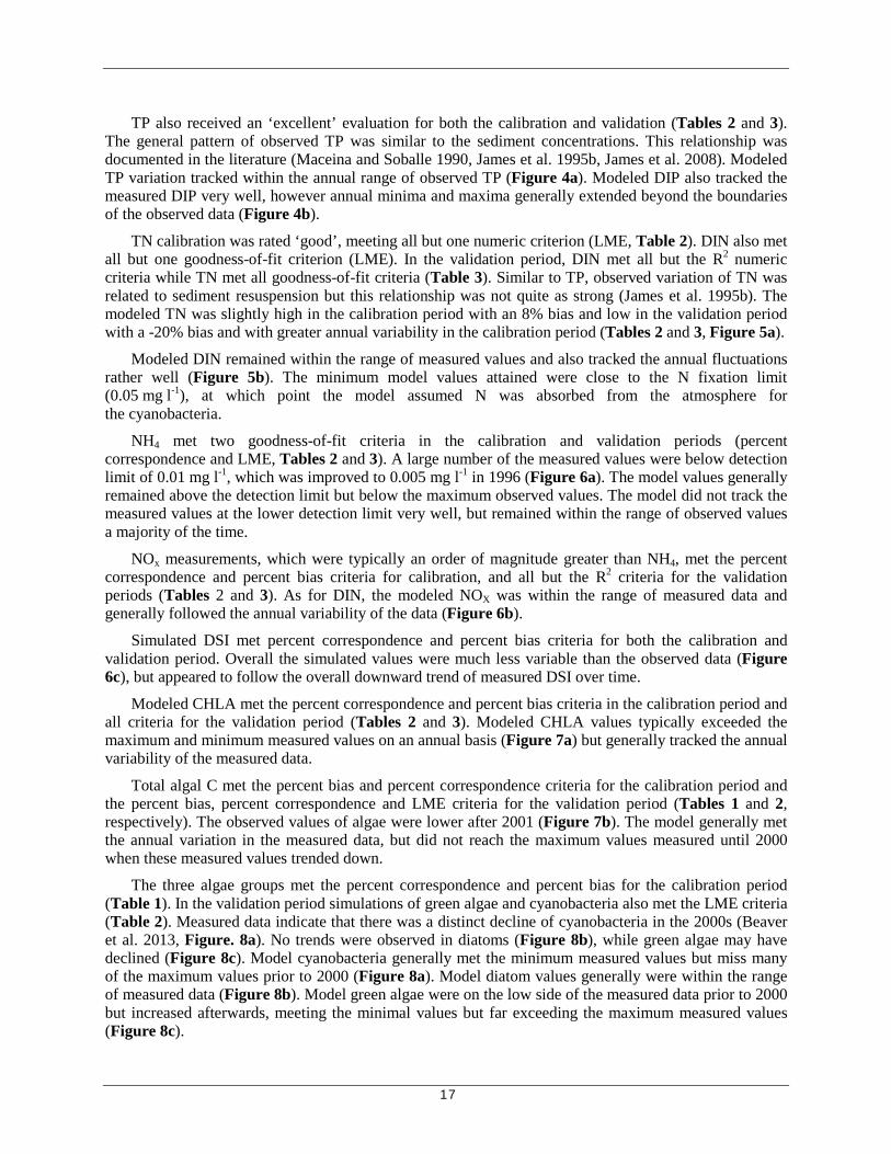
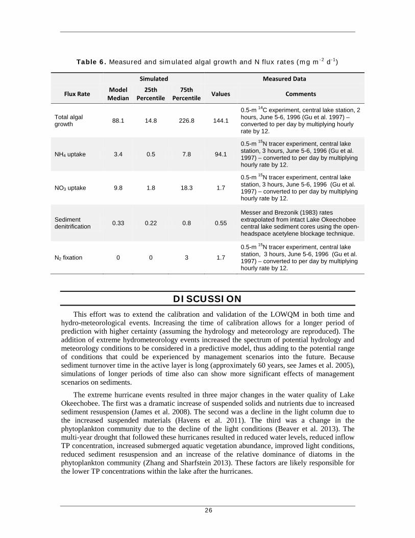
COMPARISON TO MEASURED RATES Algal growth, uptake of NH4, NO3, and N2 fixation were measured on the lake using 15N and

14C tracers (Gu et al. 1997). These measured values taken at 0.5 m in the center of the lake. In addition, denitrification estimates were measured from sediment cores by Messer and Brezonik (1983). These measurements were compared to the median, 25th and 75th percentile of the simulated daily values from the LOWQM model. The measured values fell within the percentile ranges simulated by the model for all but the NH4 uptake (Table 6)

25

Table 5. Observed (from raw data of Fisher et al. 2001, Olila et al. 1995, Reddy 1991 and BEM and University of Florida 2007) and predicted mean and standard deviations for sediments of Lake Okeechobee mg l-1 for the top 6 cm of sediment. (Note: O –

observed, S –simulated, sd – standard deviation. Bold indicates the result is within one standard deviation of the observed mean. Bold underline indicates the result is within two standard deviations of the observed mean.)

1988 1998 2006

Value O Osd S O Osd S O Osd S

Inorganic Solids 184,464 242,206 248,257 263,814 265,447 247,019 302,662 339,126 243,489

Total Phosphorus 124 95 139 179 220 136 186 243 140

Total Nitrogen 1509 1479 1,740 1302 971 1,871 2002 1669 1,791

Dissolved Inorganic Phosphorus 0.186 0.296 0.06 0.359 0.441 0.05 0.091 0.192 0.06

Total Inorganic Phosphorus 88.9 75.4 92.92 158 250.8 84.44 156.1 241.5 90.86

Dissolved Organic Phosphorus 0.164 0.404 0.04 0.022 0.076 0.04 0.025 0.051 0.04

Particulate Organic Phosphorus 34.8 26.8 45.67 21 25.8 51.54 29.6 38.7 48.45

Particulate and Dissolved Ammonia 6.5 5.2 6.03 17.2 14.7 6.08 5.9 7.1 5.8

Dissolved Inorganic Nitrogen 2.2 1.9 0.09 2 1.6 0.2 1.1 2.2 0.27

Organic Nitrogen 1,502 1,474 1,733 1,285 956 1,864 1,996 1,662 1,784

26

Table 6. Measured and simulated algal growth and N flux rates (mg m-2 d-1)

Simulated Measured Data

Flux Rate Model Median

25th Percentile

75th Percentile Values Comments

Total algal growth 88.1 14.8 226.8 144.1

0.5-m 14C experiment, central lake station, 2 hours, June 5-6, 1996 (Gu et al. 1997) – converted to per day by multiplying hourly rate by 12.

NH4 uptake 3.4 0.5 7.8 94.1

0.5-m 15N tracer experiment, central lake station, 3 hours, June 5-6, 1996 (Gu et al. 1997) – converted to per day by multiplying hourly rate by 12.

NO3 uptake 9.8 1.8 18.3 1.7


Sediment denitrification 0.33 0.22 0.8 0.55

Messer and Brezonik (1983) rates extrapolated from intact Lake Okeechobee central lake sediment cores using the open-headspace acetylene blockage technique.

N2 fixation 0 0 3 1.7


DISCUSSION This effort was to extend the calibration and validation of the LOWQM in both time and

hydro-meteorological events. Increasing the time of calibration allows for a longer period of prediction with higher certainty (assuming the hydrology and meteorology are reproduced). The addition of extreme hydrometeorology events increased the spectrum of potential hydrology and meteorology conditions to be considered in a predictive model, thus adding to the potential range of conditions that could be experienced by management scenarios into the future. Because sediment turnover time in the active layer is long (approximately 60 years, see James et al. 2005), simulations of longer periods of time also can show more significant effects of management scenarios on sediments.

The extreme hurricane events resulted in three major changes in the water quality of Lake Okeechobee. The first was a dramatic increase of suspended solids and nutrients due to increased sediment resuspension (James et al. 2008). The second was a decline in the light column due to the increased suspended materials (Havens et al. 2011). The third was a change in the phytoplankton community due to the decline of the light conditions (Beaver et al. 2013). The multi-year drought that followed these hurricanes resulted in reduced water levels, reduced inflow TP concentration, increased submerged aquatic vegetation abundance, improved light conditions, reduced sediment resuspension and an increase of the relative dominance of diatoms in the phytoplankton community (Zhang and Sharfstein 2013). These factors are likely responsible for the lower TP concentrations within the lake after the hurricanes.

27

Simulating these hydrometeorology events resulted in overestimates of TP, TN and cyanobacteria in the original model calibration (data not shown). The recalibration effort led to improved estimates of these water quality parameters more closely matching observed values, which will result in more reliable for predictions for similar extreme circumstances in the future.

Sediment-water interactions are a major factor in the water quality dynamics of Lake Okeechobee. The annual cycle of higher regional winds in the wintertime result in greater sediment resuspension and higher sediment and nutrients in the water column during this season (Havens 1994, James et al. 2009, Maceina and Soballe 1990). Major events such as hurricanes result in more persistent increases (Havens et al. 2001, James et al. 2008). Modeling the resuspension of sediment through an external forcing function resulted in the reproduction of water column TP.

TN is not as strongly related to sediment as TP (James et al. 1995b) in part because biological processes can remove or add to the pool of TN (James et al. 2011). These include N fixation by algae (Phlips and Ihnat 1995) and denitrification (Messer and Brezonik 1983, James et al. 2011), both of which contribute significantly to the N budget (Table 4). To calibrate TN properly, mineralization rates, N fixation, and denitrification rates were tuned.

Finally, algae in Lake Okeechobee are primarily light limited (Aldridge et al. 1995). The calibration of phytoplankton C was the most difficult because the model uses constant parameters to generate the growth, nutrient and light uptake capability of three separate groups of algae (cyanobacteria, diatoms, and green) that range by an order of magnitude from the least (green) to the most (cyanobacteria) dominant. Due to these model constraints, model parameters were chosen to capture the general reduction of cyanobacteria in the 2000s while maintaining the levels of diatoms and green algae.

Based on the various comparative numerics used in the calibration and validation, the model was acceptably calibrated and validated for use in predictive simulations. Because the success of calibration of parameters was not equal, any future predictive assessments using this model should include sensitivity and uncertainty analysis (see Dilks and James 2011).

PHOSPHORUS As pointed out in the previous calibration effort (James et al. 2005), an important aspect of

long-term evaluations of sediment-water P interactions is the deposition of organic P into the sediments and the remineralization of that P to IP. Part of the concern in predicting the long-term sediment-water P interactions is the concept that seston and algae deposited to the sediments consist of organic material with a wide range of resistance to decomposition. The easily degradable fraction quickly transforms to DIP, which is available for release to the water column, while more resistant organic fractions are retained and buried into the sediment. Models with only one OP state variable assume that all of this organic material is degradable. Such models cannot accurately describe both the short-term behavior due to decomposition of the readily degradable OP fraction and the longer-term behavior due to decomposition of the moderately- to non-degradable fractions (James et al. 2005). The success of this model calibration is a result of adequately defining both within sediment and sediment-water interactions.

NITROGEN N-fixation by cyanobacteria was implemented in this model because independent

measurements indicated that this process was responsible for approximately a third of the N load to the lake (Phlips and Ihnat 1995). However, after 2004, N-fixing cyanobacteria declined in dominance (e.g., Anabaena; Beaver et al. 2013) and presumably N-fixation. This is likely due to increased light limitation because after this time the TN to TP ratio declined below ten (annual

28

average for in-lake monitoring network; data not shown) indicating even greater N limitation. To address this decline in cyanobacteria dominance, the N-fixation switch was reduced from the original 0.1 mg l-1 (James et al. 2005) to 0.05 mg l-1 resulting in a better overall fit of modeled and observed DIN than the original calibration (Table 3). With the original N-fix switch, the minimal value the model would reach was just below 0.1 mg l -1, which is well above the minimal average of the observed data (Figure 5b). Using a value of 0.5 mg l -1 for the N-fix switch resulted in DIN predictions that closely matched the minimal values of the observed data.

The difficulty of calibrating and validating NH4 is attributed to the method used by the model to determine algal uptake of DIN. In this model, preference between NOx and NH4 is based on the half-saturation uptake kinetic value for DIN and the concentrations of NH4 and NOx (Ambrose et al. 1993a). Compared to observed measurements, model uptake rates for NH4 were much smaller (Table 6). Note that this comparison is the aggregated lake model to a single point/single day in the center of the lake. However, additional measurements made by Gu et al. (1997) indicate that ammonia was taken up more rapidly than nitrate in three out of four regions of the lake measured.

SILICA SI is an important parameter for diatom growth and was included to simulate this group. The

observed and computed values for DSI, for both the calibration and validation periods (Tables 2 and 3), are far in excess of values that would limit diatom growth (0.050 mg l -1). Clearly, there is not a full understanding of SI dynamics in the lake in part because loading estimates are based on quarterly rather than monthly sampling and SI in sediments have not been measured.

ALGAE The three groups of algae simulated in this model represented approximately 93% of the algal

biomass in Lake Okeechobee (Havens et al. 1996). The difference in the calibration and validation numerics was attributed primarily to the high variation within the observed data. The percent bias, which compares the means of the observed and modeled on a monthly averaged basis, was difficult to obtain in part because there was an order of magnitude difference between the observed cyanobacteria and green algae. There also was a transition from the earlier validation period of high cyanobacteria to much lower cyanobacteria in the calibration period, which corresponded generally to a decline in the frequency of N fixation (data not shown). Diatoms and green algae were essentially unchanged. In general the model maintained the trend for diatoms while greens increased. Note that greens were still an order of magnitude less than cyanobacteria and diatoms in both the calibration and validation period.

A difficulty in the calibration was to fix parameters that clearly varied over time. For example, one constant used in the model was the C to CHLA ratio. Based on the observed data, this value should be approximately 16 mg C:CHLA in the calibration (1997–2012) period and 26 mg C:CHLA in the validation (1981–1996) period. Using three separate ratios of C:CHLA for each simulated algae, the composite model average over the two periods was 20.4 mg C:CHLA, which is very close to the average observed value for both periods.

Despite using fixed values for each algal group, the observed CHLA was acceptably calibrated and validated. The simulated CHLA results extend beyond the maximal and minimal values observed in most years resulting in the poor R2 fit (Figure 7a). The only method to constrain the algae was using the light limitation factors and the self-shading coefficients. Neither of these provided enough constraint while using reasonable values from the literature (Bowie et al. 1985). Alternative formulations that include competitive feedback for space and the addition of grazers may be useful (see Suggested Model Improvements below).

29

SEDIMENTS AND SEDIMENT WATER INTERACTIONS The average observed values of nutrients in surface sediments from the three sampling events

demonstrate the large amount of spatial variation within the lake (Table 4, observed standard deviations). For the most part, model predictions are within the standard deviations of the observed data. DIN is an exception with modeled sediment values being an order of magnitude less than the observed data. Further analysis and review are required to improve model predicted sediment DIN.

SUGGESTED MODEL IMPROVEMENTS A number of changes to the LOWQM input and code would likely improve future calibration

and verification effort by addressing current weaknesses in the model’s ability to predict phytoplankton densities:

1. Evaluation of the algal uptake preference for NH4 and NOx. Given better predictions of the uptake of each of these nutrients could lead to improved estimates of organic mineralization, denitrification and nitrification in the lake. Such information would lead to improved prediction of the effects of management activities on changes in N in the lake.

2. Improved uptake kinetic formulations. The current model assumes that C:N:P:CHLA ratios remain constant within each group of algae. There are more sophisticated models that allow these ratios to vary depending on environmental conditions (Haney and Jackson 1996) and allow for luxury uptake of nutrients resulting in variable nutrient ratios.

3. Competitive feedback (space control/refugia). A spatial/refugia control mechanism (Wiegert 1979) may be useful in the LOWQM, to improve the calibration of both the CHLA and phytoplankton values.

4. Split water column into two layers. Light penetration through most of the pelagic region of the lake is very shallow (approximately 0.2 m, Phlips et al. 1997). A surface photosynthetic layer and a deeper non-photosynthetic layer could produce more precise algal growth estimates for the lake.

5. A major assumption of the LOWQM is that sediments below 6 cm act only as a sink, not a source of material to the lake. While this assumption was reasonable in the previous calibration (James et al. 2005), the hurricane events of 2004 and 2005 resulted in the disturbance and remixing of sediments well below this depth (Jin et al. 2011). Despite this remixing, such events are quite rare (James and Pollman 2011), and the material, which contains mostly unavailable P, is settled out and is reburied. The depth assumption should be reevaluated for long-term (50+ year) predictions through the addition of another deeper sediment layer, or a boundary condition that produces imports to the model under extreme (hurricane) conditions.

CONCLUSIONS Calibration and validation of the LOWQM to a longer period of monitoring data allowed the

inclusion of a series of exceptional hydro-meteorological events. This inclusion and the recalibration of the model will provide more reliable predictions for management scenarios into the future. The model predicts TP well, primarily due to the strong sediment water interactions. The more complex relationships for TN and phytoplankton and the greater difficulty in adequately calibrating to observed values may be improved through future model enhancements such as improved N-fixation and algal uptake preference. Sensitivity and uncertainty analyses are

30

recommended to assess the effects of model parameters that did not perform as well as desired on prediction results for future management scenarios.

LITERATURE CITED

Aldridge F.J., E.J. Phlips and C.L. Schelske. 1995. The use of nutrient enrichment bioassays to test for spatial and temporal distributions of limiting factors affecting phytoplankton dynamics in Lake Okeechobee, Florida. Pages 177–190 in Aumen, N.G., and R.G. Wetzel (eds.), Ecological Studies of the Littoral and Pelagic Systems of Lake Okeechobee, Florida (USA), Advances in Limnology 45.

Ambrose R.B., Jr., T.A. Wool and J.L. Martin. 1993a. The Water Quality Analysis Simulation Program, WASP5, Part A: Model Documentation. United States Environmental Protection Agency, Environmental Research Laboratory, Athens, GA.

Ambrose R.B., Jr., T.A. Wool and J.L. Martin. 1993b. The Water Quality Analysis Simulation Program, WASP5, Part B: The WASP5 Input Dataset, Version 5.00. United States Environmental Protection Agency, Center for Exposure Assessment Modeling, Athens, Georgia.

Aumen N.G. and R.G. Wetzel (eds.). 1995. Ecological Studies of the Littoral and Pelagic Systems of Lake Okeechobee, Florida (USA), Advances in Limnology 45.

Beaver J.R., D.A. Casamatta, T.L. East, K.E. Havens, A.J. Rodusky, R.T. James, C.E. Tausz and K.M. Buccier. 2013. Extreme weather events influence the phytoplankton community structure in a large lowland subtropical lake (Lake Okeechobee, Florida, USA). Hydrobiologia 709(1):213-226.

BEM and University of Florida. 2007. Lake Okeechobee Sediment Quality Final Report. Submitted to South Florida Water Management District, West Palm Beach.

Bierman V.J., Jr. and R.T. James. 1995. A preliminary modeling analysis of water quality in Lake Okeechobee, Florida: Diagnostic and sensitivity analyses. Water Research 29:2767-2775.

Blasland Bouck and Lee Inc. 2001. Lake Okeechobee Sediment Management Feasibility Study. Submitted to the South Florida Water Management District, West Palm Beach, FL

Bowie G.L., W.B. Mills, D.B. Porcella, C.L. Campbell, J.R. Pagenkopf, G.L. Rupp, K.M. Johnson, P.W.H. Chan, S.A. Gherini and C.E. Chamberlain. 1985. Rates, Constants, and Kinetics Formulations in Surface Water Quality Modeling (Second Edition). United States. Environmental Protection Agency, Environmental Research Laboratory, Athens, Georgia.

Brezonik P.L. and D.R. Engstrom. 1998. Modern and historic accumulation rates of phosphorus in Lake Okeechobee, Florida. Journal of Paleolimnology 20:31-46.

Cichra M.F., S. Badylak, N. Henderson, B.H. Rueter and E.J. Phlips. 1995a. Phytoplankton community structure in the open water zone of a shallow subtropical lake (Lake Okeechobee, Florida, USA). Pages 157–175 in Aumen, N.G., and R.G. Wetzel (eds.), Ecological Studies of the Littoral and Pelagic Systems of Lake Okeechobee, Florida (USA), Advances in Limnology 45.

Dilks, D. and R.T. James. 2011. A bayesian uncertainty analysis of the Lake Okeechobee Water Quality Model: Parameter uncertainty in a highly parameterized model. Lake and Reservoir Managment 27:376-389.

31

Fisher M.M., K.R. Reddy and R.T. James. 2001. Long-term changes in the sediment chemistry of a large shallow subtropical lake. Lake and Reservoir Managment 17:217-232.

Fisher M.M., K.R. Reddy, and R.T. James. 2005. Internal nutrient loads from sediments in a shallow, subtropical lake. Lake and Reservoir Managment 21(3):338-349.

FDEP. 2001. Total Maximum Daily Load for Total Phosphorus Lake Okeechobee, Florida. Florida Department of Environmental Protection, Tallahassee, FL, submitted to United States Environmental Protection Agency, Region IV, Atlanta, GA.

Gu B., K.E. Havens, C.L. Schelske and B.H. Rosen. 1997. Uptake of dissolved nitrogen by phytoplankton in a eutrophic subtropical lake. Journal of Plankton Research 19:759-770.

Haney J.D. and G.A. Jackson. 1996. Modeling phytoplankton growth rates. Journal of Plankton Research 18:63-85.

Havens K.E. 1994. Seasonal and spatial variation in nutrient limitation in a shallow sub-tropical lake (Lake Okeechobee, Florida) as evidenced by trophic state index deviations. Arch Hydrobiology 131:39-53.

Havens K.E., N.G. Aumen, R.T. James and V.H. Smith. 1996. Rapid ecological changes in a large subtropical lake undergoing cultural eutrophication. Ambio 25(3):150-155.

Havens K.E., K-R. Jin, A.J. Rodusky, B. Sharfstein, M.A. Brady, T.L. East, N. Iricanin, R.T. James, M.C. Harwell and A.D. Steinman. 2001. Hurricane effects on a shallow lake ecosystem and its response to a controlled manipulation of water level. Science World 1:44-70.

Havens K.E. and R.T. James. 2005. The phosphorus mass balance of Lake Okeechobee, Florida: Implications for eutrophication management. Lake and Reservoir Managment 21(2):139-148.

Havens K.E., J.R. Beaver, D.A. Casamatta, T.L. East, R.T. James, P. McCormick, E.J. Phlips and A.J. Rodusky. 2011. Hurricane effects on the planktonic food web of a large subtropical lake. Journal of Plankton Research 33(7):1081-1094.

James R.T. and V.J. Bierman, Jr. 1995. A preliminary modeling analysis of water quality in Lake Okeechobee, Florida: Calibration results. Water Research 29:2755-2766.

James R.T., B.L. Jones and V.H. Smith. 1995a. Historical trends in the Lake Okeechobee ecosystem II. Nutrient budgets. Arch Hydrobiology Supplement 107:25-47.

James R.T., V.H. Smith and B.L. Jones. 1995b. Historical trends in the Lake Okeechobee ecosystem III. Water quality. Arch Hydrobiology Supplement 107:49-69.

James R.T., J. Martin, T. Wool and P.F. Wang. 1997. A sediment resuspension and water quality model of Lake Okeechobee. Journal of American Water Resource Association 33:661-680.

James R.T., V.J. Bierman, Jr, M.J. Erickson and S.C. Hinz. 2005. The Lake Okeechobee water quality model (LOWQM) enhancements, calibration, validation and analysis. Lake and Reservoir Managment 21(3):231-260.

James R.T., M.J. Chimney, B. Sharfstein, D.R. Engstrom, S.P. Schottler, T. East and K-R Jin. 2008. Hurricane effects on a shallow lake ecosystem, Lake Okeechobee, Florida (USA). Fundamental and Applied Limnology 172(4):273-287.

32

James R.T., K.E. Havens, G. Zhu and B. Qin. 2009. Comparative analysis of nutrients, chlorophyll and transparency in two large shallow lakes (Lake Taihu, P.R. China and Lake Okeechobee, USA). Hydrobiologia 627(1):211-231.

James R.T., W. Gardner, M. McCarthy and S. Carini. 2011. Nitrogen dynamics in Lake Okeechobee: Forms, functions, and changes. Hydrobiologia 669(1):199-212.

James R.T. and C.D. Pollman. 2011. Sediment and nutrient management solutions to improve the water quality of Lake Okeechobee. Lake and Reservoir Managment 27(1):28-40.

James R.T. and B. Sharfstein. 2013. Appendix 4-1: Annual Permit Report for Lake Okeechobee Water Control Structures Operation. In: South Florida Water Management District, 2013 South Florida Environmental Report – Volume I, West Palm Beach, FL.

Jin K-R, N-B Chang, Z-G Ji and R.T. James. 2011. Hurricanes affect the sediment and environment in Lake Okeechobee. Critical Reviews in Environmental Science and Technology 41(S1):382-394.

Kirby, R., C. H. Hobbs, and A. J. Mehta. 1994. Shallow stratigraphy of Lake Okeechobee, Florida: a preliminary reconnaissance. Journal of Coastal Research 10: 339-350.

Maceina M.J. and D.M. Soballe. 1990. Wind-related limnological variation in Lake Okeechobee, Florida. Lake and Reservoir Managment 6:93-100.

Mehta A.J. 1991. Lake Okeechobee Phosphorus Dynamics Study, Sediment Characterization--Resuspension and Deposition Rates. South Florida Water Management District, West Palm Beach, Florida.

Messer J. P.L. Brezonik. 1983. Comparison of denitrification rate estimation techniques in a large shallow lake. Water Research 17:631-640.

Moore P.A.J. and K.R. Reddy. 1994. Role of Eh and pH on phosphorus geochemistry in sediments of Lake Okeechobee, Florida. Journal of Environmental Quality 23:955-964.

Moore P.A.J., K.R. Reddy and M.M. Fisher. 1998. Phosphorus flux between sediment and overlying water in Lake Okeechobee, Florida: Spatial and temporal variations. Journal of Environmental Quality 27:1428-1439.

Olila O.G., K.R. Reddy and W.G. Harris. 1995. Forms and distribution of inorganic phosphorus in sediments of two shallow eutrophic lakes in Florida. Hydrobiologia 302:147-161.

Phlips E.J. and J. Ihnat. 1995. Planktonic nitrogen fixation in a shallow subtropical lake (Lake Okeechobee, Florida, USA). Pages 191–201 in Aumen, N.G., and R.G. Wetzel (eds.), Ecological Studies of the Littoral and Pelagic Systems of Lake Okeechobee, Florida (USA), Advances in Limnology 45.

Phlips E.J., M. Cichra, K. Havens, C. Hanlon, S. Badylak, B. Rueter, M. Randall and P. Hansen 1997. Relationships between phytoplankton dynamics and the availability of light and nutrients in a shallow sub-tropical lake. Journal of Plankton Research 19:319-342.

Reddy K.R. 1991. Lake Okeechobee Phosphorus Dynamics Study: Volume II Physico-chemical Properties in the Sediments. Final report submitted to South Florida Water Management District, West Palm Beach, FL.

33

Reddy K.R., Y.P. Sheng and B.L. Jones. 1995. Lake Okeechobee Phosphorus Dynamics Study. Final report submitted to the South Florida Water Management District. West Palm Beach, FL.

SAS Institute Inc. 1989. SAS/STAT® Users Guide: Version 6. SAS Institute, Cary, NC.

SFWMD. 1999. SFWMD Comprehensive Quality Assurance Plan – 1999. South Florida Water Management District, West Palm Beach, FL.

SFWMD. 2011a. Nexrad-ET. South Florida Water Management District, West Palm Beach, FL. http://my.sfwmd.gov/nexrad/arcims/default.htm. Accessed January 25, 2012.

SFWMD. 2011b. Environmental Data Management System. South Florida Water Management District, West Palm Beach, FL. Accessed June 1, 2012.

SFWMD 2012. DBHYDRO. SFWMD. 1999. SFWMD Comprehensive Quality Assurance Plan – 1999. South Florida Water Management District, West Palm Beach, FL. http://my.sfwmd.gov/dbhydroplsql/show_dbkey_info.main_menu. Accessed July 21, 2012.

Strathman R.R. 1967. Estimating the organic carbon content of phytoplankton from cell volume or plasma volume. Limnology and Oceanography 12:411-418.

RECOVER. 2007. Lake Okeechobee Performance Measure Water Quality Mosaic. Restoration Coordination and Verification program c/o United States Army Corps of Engineers, Jacksonville, FL, and South Florida Water Management District, West Palm Beach, FL. http://www.evergladesplan.org/pm/recover/recover_docs/et/lo_pm_waterquality.pdf. Accessed march 7, 2013.

Thomann R.V. and J.A. Mueller. 1987. Principles of Surface Water Quality Modeling and Control. Harper and Row Publishers, New York, NY.

USACE. 1978. Area Capacity Curve-Lake Okeechobee 1968, Plates 26A and 27 – Central and Southern Florida Project for Flood Control and Other Purposes 2. Part 1. Rule Curves and Key Operating Criteria, Master Regulation Manual. United States Army Corps of Engineers, Jacksonville, FL.

Wiegert R.G. 1979. Population Models: Experimental Tools for Analysis of Ecosystems. Pages 233–277 in Horn D.J., G.R. Stairs and R.D. Mitchell (eds.), Analysis of Ecological Systems, Ohio State University Press, Columbus, Ohio.

Zhang J., and B. Sharfstein. 2013. Chapter 8: Lake Okeechobee Watershed Protection Program. In: South Florida Water Management District, 2013 South Florida Environmental Report –. Volume I. West Palm Beach, FL.

http://www.evergladesplan.org/pm/recover/recover_docs/et/lo_pm_waterquality.pdf

34

Appendix A. Phosphorus-Related Parameters

35

Parameter Model Calibration

Organic Phosphorus Class

Readily Degradable

Moderately Degradable

Non-Degradable Dissolved Description

KOPi original 0.031 0.0034 0 0.031 Mineralization rate of

organic P (/day) new 0.022 0.0024 0 0.01

KSOPi original 0.014 0.0014 0 0.014 Mineralization rate of

organic P in sediments (/day) new 0.011 0.018 0 0.005

VO

original 6.700 6.7 6.7 Settling of organic

nutrients new 9.500 9.5 9.5 Not

available (NA)

XOPi

original 0.600 0.1 0.1 0.2 Fraction of algal P that is recycled to this form of organic P (mg P/mg

Algal P) new 0.400 0.3 0.15 0.15

ΘOPi original 1.060 1.06 NA 1.06 Temperature coefficient

for mineralization (unitless) new 1.060 1.06 NA 1.06

ΘSOPi original 1.060 1.06 NA 1.06 Temperature coefficient

for mineralization in sediments (unitless) new 1.060 1.06 NA 1.06

ΦOPi

original 0.150 0.15 NA NA Fraction mineralized to dissolved organic P in

water column (mg dissolved organic P/mg

organic P) new 0.100 0.1 NA NA

ΦSOPi

original 0.150 0.15 NA NA Fraction mineralized to dissolved organic P in

sediments (mg dissolved organic P/mg

organic P) new 0.100 0.1 NA NA

36

Appendix B. Original and New Calibration of Phytoplankton

Parameters

37

Parameter Calibration Cyano-bacteria Diatoms Green

Algae Description

CCHL original 22 29 22

C to CHLA ratio (mg C mg-1 CHLA) new 16 24 21

FON original/new 0.5 0.5 0.5 Fraction of N that recycles to organic pool (mg organic N mg-1 TN)

FOP original/new 0.5 0.5 0.5 Fraction of P that recycles to organic pool (mg organic P mg-1 TP)

FSAP original/new NA 0 NA Fraction of SI that is dissolved (mg DSI mg-1 Total SI)

G1max original 1.5 2 2

Maximum growth rate d-1 new 1.7 2.2 2

IS1 original/new 45 100 105 Maximum light saturation Langleys d-1

kN original/new 0.032 0.032 0.032 Half saturation for DIN

kP original/new 0.0032 0.0032 0.0032 Half saturation for DIP

KPZDC original/new 0.02 0.02 0.02 Decomposition rate of phytoplankton in sediment day-1

KPZDT original/new 1.06 1.06 1.06 Temperature coefficient of phytoplankton decomposition in sediments (unitless)

kSI original/new NA 0.05 NA Half saturation for DSI (mg SI l-1)

N2FIX original 0.1 NA NA

N fixation switch (mg DIN l-1) new 0.06 NA NA

NCRB original/new 0.125 0.125 0.125 N to C Ratio (mg N mg-1 C)

PCRB original/new 0.022 0.022 0.022 P to C Ratio (mg P mg-1 C)

SICARB original/new NA 1 NA SI to C Ratio (mg Si mg-1 C)

Va original 4.32 9.43 8.49

Algal settling rate (cm d-1) new 4.75 12.1 10.97

ηphyt original 0.029 0.021 0.023 Algal light extinction coefficient (m-1 mg-1

CHLA) new 0.028 0.02 0.023

Θ1 original/new 1.06 1.06 1.06 Temperature coefficient for algal growth (unitless)

Θr original/new 1.06 1.06 1.06 Temperature coefficient for respiration (unitless)

λd original 0.02 0.053 0.056

Non-predatory mortality (d-1) new 0.02 0.055 0.054

λr original 0.087 0.072 0.072

Respiration rate (d-1) new 0.078 0.063 0.056

38

Appendix C. Additional Original and New Calibration Parameters

39

Parameter Original New Parameter Description

DSS 0.00008 N/C Diffusion rate between surface and bottom sediments (m2 second-1)

DWS 0.00008 N/C Diffusion rate between water column and sediment segment (m2 sec-1)

FDON 0.002 N/C Fraction of organic N that is dissolved (mg DON mg-1 ON)

KBOD 0.5 N/C Half saturation coefficient of oxygen (O2) limitation (mg O2 l-1) for the decay rate of organic C

KDC 0.1 N/C Carbonaceous deoxygenation rate constant (d-1) KDENIT 0.14 0.08 Maximum denitrification rate at 20 degrees Celsius (ºC) (d-1) KPSPAV 1000 N/C Partition coefficient between DIP and anaerobic sediments kg l-1 KPSPOV 6000 N/C Partition coefficient between DIP and aerobic sediments kg l-1

KNIT 0.4 0.3 Maximum nitrification rate at 20 ºC (day-1) KNO3 0.1 N/C Denitrification half-saturation factor (mg O2 l-1) KON 0.0045 0.0011 Maximum organic N mineralization at 20o C (d-1) KONs 0.000045 0.000040 maximum organic N mineralization at 20o C in the sediment (d-1)

KOXNIT 1 N/C Nitrification half saturation (mg l-1) KPSi 0.1 N/C Solubilization of particulate silica (d-1) KPSN 30 N/C Partition coefficient between ammonium and sediment (kg l-1) KPSSI 110 N/C Partition coefficient between available SI and sediment (kg l-1) LDIP 72.5 N/C Atmospheric load of IP (kg d-1)

LISS 1130000 N/C Additional load of solids (as calcium carbonate [CaCO3]) to surface sediment (kg d-1)

LNH4 661.7 N/C Atmospheric load of ammonia (kg d-1) LNOX 714.6 N/C Atmospheric load of NOx (kg d-1) LON 2003 N/C Atmospheric load of organic N (kg d-1) LOP 23.3 N/C Atmospheric load of organic P (kg d-1)

OCRB 2.67 N/C Oxygen to C ratio (mg 02 mg-1 C) SMIX 0.03 N/C Solids mixing between sediment segments (cm d-1)

Vb 0.095 N/C Burial rate of sediments cm per year Viss 59.3 N/C Settling of suspended solids cm per day Ηss 0.215 0.315 Light extinction coefficient due to suspended solids (m•mg ISS l-1)-1 Ηw 2.83 1.7 Light extinction coefficient due to color in water (m-1) ΘD 1.06 N/C Temperature coefficient for diffusion rates (unitless) ΘDC 1.06 N/C Temperature coefficient for carbonaceous deoxygenation (unitless) ΘDENIT 1.06 N/C Temperature coefficient for denitrification (unitless) ΘNIT 1.06 N/C Temperature coefficient for nitrification (unitless) Θon 1.06 N/C Temperature coefficient for organic N mineralization (unitless) Θons 1.06 N/C Temperature coefficient for N mineralization in sediment (unitless) Θpsi 1.06 N/C Temperature coefficient for SI solubilization (unitless) ΘSMIX 1.06 N/C Temperature coefficient for solids mixing (unitless)

N/C – no change

The Lake Okeechobee Water Quality Model (LOWQM) · EXECUTIVE SUMMARY The Lake Okeechobee Water...

Documents

Transcript of The Lake Okeechobee Water Quality Model (LOWQM) · EXECUTIVE SUMMARY The Lake Okeechobee Water...