The Lagrangian particle method for macroscopic andmicro±macro viscoelastic flow computations1

P. Halin, G. Lielens, R. Keunings*, V. Legat

CESAME, Division of Applied Mechanics, Universite catholique de Louvain, B-1348 Louvain-la-Neuve, Belgium

Received 4 March 1998; revised 12 May 1998

Abstract

We propose a new numerical technique, referred to as the Lagrangian Particle Method (LPM), for computing time-

dependent viscoelastic flows using either a differential constitutive equation (macroscopic approach) or a kinetic theory model

(micro±macro approach). In LPM, the Eulerian finite element solution of the conservation equations is decoupled from the

Lagrangian computation of the extra-stress at a number of discrete particles convected by the flow. In the macroscopic

approach, the extra-stress carried by the particles is obtained by integrating the constitutive equation along the particle

trajectories. In the micro±macro approach, the extra-stress is computed by solving along the particle paths the stochastic

differential equation associated with the kinetic theory model. Results are given for the start-up flow between slightly

eccentric rotating cylinders, using the FENE and FENE-P dumbbell models for dilute polymer solutions. # 1998 Elsevier

Science B.V. All rights reserved.

Keywords: Finite element method; Stochastic simulation; FENE dumbbells

1. Introduction

To date, most numerical simulations of viscoelastic flows have been based on a purely macroscopic

approach where one solves numerically the conservation laws together with a suitable rheologicalconstitutive equation. Study of the monograph by Crochet, Davies and Walters [1] and of consecutivereview papers (e.g. [2±5]) reveals that progress in macroscopic viscoelastic flow computations has beenvery impressive indeed. The subject, however, is by no means closed and further developments are stillcalled for, such as improved techniques for time-dependent and three-dimensional flows. Since thepioneering work by Laso and OÈ ttinger [6,7], a complementary micro±macro approach to viscoelasticflow simulations is now emerging that combines the solution of the conservation laws with the directuse of a kinetic theory model describing the fluid's rheology (e.g. [8±12]). In the micro±macro

J. Non-Newtonian Fluid Mech. 79 (1998) 387±403

ÐÐÐÐ

* Corresponding author. Tel.: +32-10-47-23-50; fax: +32-10-47-21-80.1Dedicated to Professor Marcel J. Crochet on the occasion of his 60th birthday.

0377-0257/98/$ ± see front matter # 1998 Elsevier Science B.V. All rights reserved.

PII: S 0 3 7 7 - 0 2 5 7 ( 9 8 ) 0 0 1 2 3 - 2

approach, modeling is achieved at the coarse-grain level without resorting to closure approximations ofquestionable value, thus providing a direct link between the flow-induced development of themicrostructure and the flow operating conditions.

In the present paper, we propose a new numerical technique, referred to as the Lagrangian ParticleMethod (LPM), for solving time-dependent viscoelastic flows with either the macroscopic or themicro±macro approach. LPM combines in a decoupled fashion the solution of the conservation lawswith a Lagrangian computation of the extra-stress at a number of discrete particles that are convectedby the flow. The extra-stress is computed by integrating along the particle paths either the relevantdifferential constitutive equation (macroscopic approach), or the stochastic differential equationassociated to the kinetic theory model (micro±macro approach). For illustrative purposes, we considerthe start-up flow of a dilute polymer solution between slightly eccentric rotating cylinders. The polymersolution is described by the kinetic theory of finitely extensible non-linear elastic (FENE) dumbbells.The FENE theory is used as such in the micro±macro LPM simulations, while its approximatemacroscopic version, namely the FENE-P constitutive equation obtained with the Peterlin closureapproximation [13], is used in the macroscopic LPM runs. In the micro-macro LPM simulations, eachLagrangian particle convected by the flow carries an ensemble of dumbbells. In LPM, these ensemblesof dumbbells can be statistically uncorrelated or correlated. The latter case yields in fact a numericalapproach that is equivalent, in the limit of vanishing discretization error, to the method of Brownianconfiguration fields introduced recently by Hulsen et al. [11].

The paper is organized as follows. In Section 2, we detail the relevant governing equations. Section 3describes the basic technical features of LPM. The simulation results are reported in Section 4. Finally,we conclude in Section 5.

2. Governing equations

We consider the time-dependent isothermal flow of an incompressible viscoelastic fluid in a confinedgeometry. Expressed in Eulerian form, the conservation laws for linear momentum and mass read [14]

�Dv

Dt� r � �ÿpI � s�; (1)

r � v � 0; (2)

where � is the density, p and v are the pressure and velocity fields, respectively, I is the unit tensor, s isthe extra-stress tensor, and �Dv=Dt� is the material time derivative �@v=@t� � v � rv. Note that we haveneglected body forces in Eq. (1). For describing the rheology of polymer solutions, it is customary todefine the extra-stress s as the sum of a viscous solvent contribution ss and a polymer contribution sp,

s � ss � sp; ss � 2�sD; (3)

where D is the rate of deformation tensor 12�rv�rvT� and �s is the constant shear viscosity of the

solvent.The conservation laws Eqs. (1) and (2) must be closed with a suitable model that relates the polymer

stress sp to the deformation of the fluid. In the present paper, we adopt for that purpose the kinetictheory of Warner finitely extensible non-linear elastic (FENE) dumbbells [13]. In this framework, the

388 P. Halin et al. / J. Non-Newtonian Fluid Mech. 79 (1998) 387±403

polymer solution is viewed as a suspension of non-interacting dumbbells convected in a Newtoniansolvent. A dumbbell is made of two identical Brownian beads connected by a spring. While the beadsrepresent the interaction between the polymer and the solvent, the spring models intramolecularinteractions. Carried by the macroscopic flow, the beads experience Brownian force, Stokes drag andthe spring force. In this coarse grain picture, the configuration of the polymer is described by the lengthand orientation of the vector Q connecting the two beads. For FENE dumbbells, the spring force Fc isdefined as

Fc�Q� � H

1ÿ Q2=Q20

Q; (4)

where H is a spring constant and Q0 is the maximum spring length. Although quite simple, the kinetictheory of FENE dumbbells has been found recently to model many phenomena observed with dilutesolutions (e.g. [15,16]). In particular, it is able to predict hysteretic behaviour in stress growth/relaxation experiments [17±19].

A central result of kinetic theory [13] is the diffusion equation that governs the evolution of theconfiguration distribution function �Q; t�, namely

@

@t� ÿ @

@Q� j � Qÿ 2

�Fc�Q�

� �

� �� 2kT

�

@

@Q� @@Q

; (5)

where � is the friction coefficient of the Brownian beads, T is the absolute temperature, k is theBoltzmann constant, and j is the velocity gradient. The latter is assumed constant over the polymer(dumbbell) length scale. In non-homogeneous flows, the distribution function generally depends uponthe spatial position x, and the time derivative in Eq. (5) becomes in fact the material derivativeD =Dt � @ =@t � v � @ =@x. A second key result of kinetic theory is an expression due to Kramers[13] that yields the polymer contribution to the stress:

sp � ÿnkTI � nhQFc�Q�i; (6)

where n is the dumbbell number density and the angular brackets denote the configuration spaceaverage

h�i �Z� dQ: (7)

For Hookean dumbbells (i.e. Q0!1 in Eq. (4)), it is possible to derive from Eqs. (5) and (6) a closed-form constitutive equation for the polymer stress sp. This yields the Oldroyd-B model, with a relaxationtime � � �/4H and a polymer contribution to the shear viscosity �p�nkT� [13]. When Q0 has a finitevalue, however, it is impossible to obtain a macroscopic constitutive equation that is mathematicallyequivalent to the FENE kinetic model. In order to exploit Kramers' expression Eq. (6), one must eithersolve the diffusion Eq. (5), or, as done in the present work, integrate along the flow trajectories theassociated Itoà stochastic differential equation [20]:

dQ � j � Qÿ 2

�Fc�Q�

� �dt �

��������4kT

�

sdW: (8)

P. Halin et al. / J. Non-Newtonian Fluid Mech. 79 (1998) 387±403 389

Here, W is the three-dimensional Wiener process, namely a Gaussian stochastic process with vanishingmean and covariance hW�t1�W�t2�i � min�t1; t2�I. As discussed in [20], Eq. (8) is an evolutionequation for the Markovian process Q whose probability density is solution of the diffusion Eq. (5).In the stochastic simulation approach, the polymer stress sp is again obtained by means of Kramers'expression Eq. (6), with the configuration average Eq. (7) computed as an ensemble average over manyrealizations of the stochastic process Q.

In the present paper, we also propose a new approach to the numerical computation of viscoelasticflow problems with a differential constitutive equation. The FENE-P equation is used for illustrativepurposes. It is based on a self-consistent pre-averaging approximation of the spring force Eq. (4) due toPeterlin,

Fc�Q� � H

1ÿ hQ2i=Q20

Q: (9)

The Peterlin closure approximation allows one to derive from the diffusion Eq. (5) the followingevolution equation [13] for the configuration tensor A � hQQi:

@A

@t� v � rAÿ j � Aÿ A � jT � 4kT

�I ÿ 4H=�

1ÿ Tr�A�=Q20

A: (10)

Use of Kramers' expression Eq. (6) and of the force law Eq. (9) then yields the FENE-P polymer stressin terms of the configuration tensor:

sp � ÿnkTI � nH

1ÿ Tr�A�=Q20

A: (11)

As detailed in [13], Eqs. (10) and (11) lead to a non-linear differential constitutive equation for thepolymer stress sp. In numerical work, it is more convenient to solve the configuration Eq. (10), and thencompute the polymer stress using Kramers' expression Eq. (11).

The rheometrical responses of the FENE and FENE-P models are compared in [21,22], where it isshown that the Peterlin closure approximation can have a significant impact indeed. (For a markedlybetter closure approximation of the FENE theory, see [17].) The FENE and FENE-P models involve atime constant � � �/4H and the dimensionless finite extensibility parameter b � HQ2

0=kT. We also notefor further reference that the polymer contribution to the zero shear rate viscosity is�0

p � nkT�b=�b� 3� for the FENE-P fluid, and �0p � nkT�b=�b� 5� for the FENE theory.

3. The Lagrangian particle method

3.1. Basic features

The LPM is depicted schematically in Fig. 1. We decouple the Eulerian solution of the conservationEqs. (1) and (2) from the Lagrangian computation of the polymer contribution to the stress. A typicaltime step goes as follows. Using the current polymer stress values, computed in each element (at theprevious time step), a standard Galerkin finite element technique is applied to the conservationequations to yield the updated velocity and pressure fields. The new velocity field is then used to update

390 P. Halin et al. / J. Non-Newtonian Fluid Mech. 79 (1998) 387±403

the polymer stress. In LPM, we compute the polymer stress at discrete Lagrangian particles which areconvected by the flow. This is achieved by solving along the computed particle trajectories either themacroscopic constitutive Eqs. (10) and (11), or the stochastic differential Eq. (8) for a larger number ofdumbbells carried by each particle. The polymer stress values thus obtained at the Lagrangian particlesare converted into an Eulerian, element-by-element polynomial representation, which feeds thediscretized conservation laws and allows for the calculation of the velocity and pressure fields at thenext time step.

Let us now briefly review the main technical features of LPM.

3.2. Conservation equations

We consider time-dependent, two-dimensional (2D) flows in a domain with a known boundary@. The flow domain is discretized by means of a fixed mesh of finite elements, over which theEulerian velocity and pressure fields are approximated as

va�x; t� �XNv

i�1

vi�t� i�x�; pa�x; t� �XNp

j�1

pj�t��j�x�: (12)

Here i and �j are given finite element basis functions, while vi and pj are unknown, time-dependentnodal values. The mesh being fixed, the shape functions depend on the spatial coordinates x only. Weuse Galerkin's principle (e.g. [3]) to discretize the conservation laws Eqs. (1) and (2). Residualsobtained after substitution of the approximations Eq. (12) in the governing Eqs. (1) and (2) are madeorthogonal to the set of basis functions, and an integration by parts is performed in the discretized

Fig. 1. Schematic of the Lagrangian particle method.

P. Halin et al. / J. Non-Newtonian Fluid Mech. 79 (1998) 387±403 391

momentum balance. The Galerkin equations readZ

i �Dva

Dt

� �d �

Z

r Ti � �ÿpaI � 2�sD

a � sp� d �Zq

it ds; (13)Z

�j�r � va�d � 0; (14)

for 1� i � N� and 1 � j � Np. In Eqs. (13) and (14), every term with the superscript a denotes thecorresponding finite element approximation obtained from the expansions Eq. (12), t is the contactforce, and s the arc length measured along the boundary.

The Galerkin Eqs. (13) and (14) can be used to compute the velocity and pressure fields provided thepolymer stress contribution to the discretized momentum balance Eq. (13), namelyZ

r Ti � sp d; (15)

be known. In LPM, we treat Eq. (15) as a known pseudo-body force term. The Galerkin Eqs. (13) and(14) thus constitute a set of first-order differential equations for the nodal values of va and pa. In thecurrent implementation of LPM, we discretize Eqs. (13) and (14) in time using the Euler forward/Eulerbackward predictor-corrector scheme with a constant time step �tcons. The solution of the implicitEuler backward equations is obtained by means of Newton's scheme, the initial guess being providedby the explicit Euler forward prediction. Finally, we use biquadratic continuous basis functions for thevelocity, and bilinear continuous basis functions for pressure.

3.3. Tracking the motion of Lagrangian particles

In LPM, we compute the polymer stress sp at a number Npart of Lagrangian particles convected by theflow. Over a typical time step �tn; tn�1 � tn ��tcons�, the trajectory of each Lagrangian particle isdetermined using the Eulerian velocity field obtained at time tn. If s denotes the position vector of theparticle, one thus solves the kinematic equation

dr

dt� va�r; tn�; (16)

for t in �tn; tn�1� and with the initial condition r(tn) known from the previous time step. We integrate Eq.(16) by means of the tracking procedure proposed by Goublomme et al. [23] in the context of steady-state flows of integral viscoelastic fluids. The basic idea is to solve Eq. (16) in the parent finite element,using a fourth-order Runge±Kutta method. For this, we adopt a constant time step �ttrack such that�ttrack � �tcons. Knowledge of the particle trajectories between tn and tn�1 allows us to compute thepolymer stress sp at time tn�1, as we now explain.

3.4. Differential constitutive equation

Most differential constitutive models currently used in computational rheology have the form

Dsp

Dt� f �sp;j�: (17)

392 P. Halin et al. / J. Non-Newtonian Fluid Mech. 79 (1998) 387±403

With microstructural models such as the FENE-P equation, the evolution equation for the configurationtensor (see Eq. (10)) has a similar form:

DA

Dt� g�A;j�: (18)

In LPM, we solve Eq. (17) or Eq. (18) along the flow trajectory of the Npart Lagrangian particles. Thematerial derivative operator thus reduces to a simple time derivative taken along the pathlines. Over atypical time step �tn; tn�1 � tn ��tcons�, we use the Eulerian velocity field obtained at time tn tointegrate Eq. (17) or Eq. (18). With the FENE-P model, one thus solves for each particle

DA�r�t��Dt

� g�A�r�t��; ja�r�t�; tn��; (19)

along the trajectory fr�t�; t 2 �tn; tn�1�g and with the initial condition A�r�tn�� known from the previoustime step. For this, we use a fourth-order Runge±Kutta method with a constant time step �tconst suchthat �ttrack��tconst��tcons. Having obtained A�r�tn�1��, we compute the updated polymer stresssp�r�tn�1�� by means of Kramers' expression (11).

3.5. Kinetic theory model

Computation of the polymer stress with the kinetic dumbbell model is achieved by solving thestochastic differential Eq. (8) along the trajectory of the Npart Lagrangian particles. For simplicity, wewrite all subsequent equations in dimensionless form. The connector vector Q, the time t, the velocitygradient and the polymer stress sp are made dimensionless with �kT=H�1=2; �; �ÿ1, and nkT,respectively, and we define the notation h�x� � 1=�1ÿ x=b�. For FENE dumbbells, the dimensionlessconnector force reads

Fc�Q� � h�Q2�Q; (20)

while for FENE-P dumbbells we have

Fc�Q� � h�hQ2i�Q: (21)

Finally, the dimensionless Kramers' expression Eq. (6) is

sp � hQFci ÿ I: (22)

Each Lagrangian particle carries a number Nd of dumbbells. Over the time step �tn; tn�1 � tn ��tcons�,the configuration Q of each dumbbell is obtained by solving Eq. (8) using the Eulerian velocity field attime tn,

dQ�r�t�� � �ja�r�t�; tn� � Q�r�t�� ÿ 12Fc�Q�r�t���� dt � dW; (23)

along the trajectory fr�t�; t 2 �tn; tn�1�g and with the initial condition Q�r�tn�� known from the previoustime step. In view of Kramers' expression Eq. (22), the updated polymer stress carried by a particle isthen approximated by the ensemble average

P. Halin et al. / J. Non-Newtonian Fluid Mech. 79 (1998) 387±403 393

sp�r�tn�1�� � 1

Nd

XNd

i�1

Q�i��r�tn�1��Fc�Q�i��r�tn�1��� ÿ I; (24)

where Q�i� is an individual realization of the stochastic process Q, and Fc is evaluated using either theFENE Eq. (20) or FENE-P Eq. (21) spring law.

For FENE-P dumbbells, we integrate Eq. (23) by means of the explicit Euler±Maruyamascheme, using a constant time step �tstoch such that �ttrack��tstoch��tcons. This yields the simplerecurrence

Q�r�tj�1�� � Q�r�tj�� � �ja�r�tj�; tn� � Q�r�tj�� ÿ 12Fc�Q�r�tj�����tstoch ��W j; (25)

for tj�1 � tj ��tstoch in the interval �tn; tn�1�. The vector of Wiener increments �W j has independentGaussian components with zero mean and variance �tstoch.

The Euler±Maruyama scheme Eq. (25) is of weak order 1 [20]. When used with FENE dumbbells, itcan lead to difficulties if �tstoch is too large. Indeed, an individual dumbbell can have its dimensionlesslength become larger than the upper bound

���bp

, which is unphysical. Thus, for FENE dumbbells, wesolve Eq. (23) by means of the semi-implicit predictor±corrector scheme proposed by OÈ ttinger [20].The predictor is the Euler scheme (25), which gives ~Q�r�tj�1��. The corrector has the form

�1� 14h�Q2�r�tj�1����tstoch�Q�r�tj�1�� � d�Q�r�tj��; ~Q�r�tj�1��;�W j�; (26)

where the known vector d is given by

d � Q�r�tj�� � 12�ja�r�tj�1�; tn� � ~Q�r�tj�1�� � ja�r�tj�; tn� � Q�r�tj��

ÿ 12h�Q2�r�tj���Q�r�tj����tstoch ��W j: (27)

The update Q�r�tj�1�� is a vector with direction d and length q that is solution of a cubic algebraicequation derived from Eq. (26). As shown in [20], q is unique and always in �0; ���

bp �. The predictor±

corrector scheme Eqs. (26) and (27) is of weak order 2.In Eqs. (25)±(27), the Gaussian increments �Wj can be replaced by other random variables that are

cheaper to generate. As in [22], we use uniformly distributed random numbers whose moments areselected such as to keep unchanged the weak order of the numerical schemes [20].

An important issue to consider is that of the statistical correlation between ensembles of dumbbellscarried by neighboring Lagrangian Particles [24]. The standard approach [7] uses uncorrelatedensembles in the sense that Npart�Nd independent Wiener processes govern the stochastic evolution ofthe dumbbells. Alternatively, if the same initial ensemble of dumbbells is used in each Lagrangianparticles, and if the same Nd independent Wiener processes are generated to compute the configurationof corresponding dumbbells in each particle, then strong correlations develop in the polymer stressfluctuations at neighboring particles, which have almost identical flow histories. As discussed in [24],variance reduction should result from the cancellation of these fluctuations when taking the divergenceof the polymer stress in the momentum balance Eq. (1). Use of correlated ensembles of dumbbells isthe basic idea behind the method of Brownian configuration fields introduced by Hulsen et al. [11]. Asdiscussed in [11,24], it dramatically reduces the spatial fluctuations of the computed velocity and stressfields, while decreasing the cost of generating the random numbers. In fact, LPM with correlatedensembles of dumbbells can de viewed as a Lagrangian particle solution of Eq. (11) in [11] that governs

394 P. Halin et al. / J. Non-Newtonian Fluid Mech. 79 (1998) 387±403

a particular configuration field. Their number Nf of configuration fields thus corresponds to our numberNd of dumbbells carried by each lagrangian particle.

3.6. Computation of the polymer stress integral

At the end of a typical time step for the solution of the conservation laws, say at time tn�1, we thus,have at our disposal values of the polymer stress sp at discrete Lagrangian Particle located at rl�tn�1�,for l � 1; 2;��� ;Npart. The last computational task to discuss is that using out these Lagrangian results tofeed the Eulerian discretized momentum balance Eq. (13). In other words, one must compute thepolymer stress integral Eq. (15) that will be used in the momentum balance Eq. (13) to update thevelocity field at time tn�2 � tn�1 ��tcons.

To do so, we compute in each finite element the linear least-squares polynomial that best fits theavailable polymer stress data, on the basis of the Lagrangian particles that are found present in theelement at time tn�1. The resulting piecewise-continuous Eulerian representation of sp is then used toevaluate the integrand of Eq. (15) at all integration points of the finite element mesh. Clearly, thisprocedure requires that at least three Lagrangian particles be present in each element at all discretetimes when the polymer stress integral is evaluated.

4. Results for start-up flow in a journal bearing

4.1. Problem description

We consider the time-dependent, planar flow of FENE and FENE-P fluids between slightly eccentriccylinders, starting from the rest state (Fig. 2). The inner cylinder, of radius Ri, is rotating at a constantangular velocity !, while the outer cylinder, of radius Ro, is fixed. The axes of the two cylinders areseparated by a small eccentricity e. We assume that the fluid sticks to the cylinder walls, and specify therest state as initial conditions. Thus, ma�x; t � 0� is set to 0 over . When using the macroscopic FENE-P constitutive equation, the initial configuration tensor A is set to its equilibrium value identically (thisamounts to specifying sp�x; t � 0� � 0 over . In the stochastic simulations, the initial dumbbellconfigurations in each Lagrangian particle are generated using the equilibrium distribution function[13].

The particular flow parameters and material data used in this work are listed in Table 1. The presentflow problem is characterized by the dimensionless eccentricity � � e=�Ro ÿ Ri� � 0:1, the dimension-less thickness � � �Ro ÿ Ri�=Ri � 0:1, the Reynolds number Re � �!Ri�Ro ÿ Ri�=��s � �0

p� � 1:1, theDeborah number De � �!Ri=�Ro ÿ Ri� � 3, the dimensionless finite extensibility b�50, and theviscosity ratio � � �s=��s � �0

p� � 1=9.

Table 1

Flow parameters and material data used in the simulations (expressed in an arbitrary consistent system of units)

Flow parameters Ri�10 Ro�11 e�0.1 !�0.1

Material data ��3 b�50 ��0.1 �s�0.1 �0p�0.8

P. Halin et al. / J. Non-Newtonian Fluid Mech. 79 (1998) 387±403 395

A typical finite element mesh is shown in Fig. 2. We use structured grids with Nr � N� quadrilateralelements, where Nr and N� are the number of uniformly-distributed elements in the radial and azimuthaldirections respectively. Most numerical results shown in this section have been obtained with the 4�80mesh of Fig. 2. For validation purposes, computations have also been performed with 8�80 and 4�160meshes, with identical results at the scale of the figures shown here [25]. The numerical solutions willbe presented in terms of the temporal evolution of the velocity and polymer stress in the region ofnarrowest gap (Fig. 2).

4.2. Macroscopic LPM computations with the FENE-P model

The results obtained with LPM applied to the FENE-P constitutive model Eqs. (10) and (11) areshown in Fig. 3. Contrary to the Newtonian solution (Re�1.1, De�0), the FENE-P velocity component�y reaches its steady value in an oscillatory fashion. A similar behaviour is predicted for thecomponents of the polymer stress. These LPM results have been obtained with a total of Npart � 2880Lagrangian particles that were uniformly distributed (i.e. 9 per element) at time t�0. The time stepswere set to �tcons � 10ÿ2 and �ttrack � �tconst � 10ÿ3.

In order to validate the LPM results, we have also computed the FENE-P solution using the mixedfinite element method implemented by Purnode and Crochet [26]. In this method, the Galerkinprinciple is applied to both the conservation and constitutive equations. Quadrilateral elements are usedwith linear, quadratic and 4�4 linear sub-elements for the pressure, the velocity and the configurationtensor, respectively. The time stepping scheme is the Euler predictor-corrector method. Fig. 3 shows theresults obtained with the mixed method, using the mesh of Fig. 2 and a time step �t �10ÿ2. Theagreement with the results provided by LPM is excellent.

Fig. 2. Finite element mesh for computing the start-up flow in a journal bearing. The enlargement shows a number of

Lagrangian particles convected by the flow, as well as the locations where the computed polymer stress (�) and velocity (*)

are displayed in subsequent figures.

396 P. Halin et al. / J. Non-Newtonian Fluid Mech. 79 (1998) 387±403

4.3. Micro±macro LPM computations with FENE-P dumbbells

Before discussing results for the FENE kinetic theory, it is useful to evaluate the stochastic LPMapproach with FENE-P dumbbells. We plot in Fig. 3 the FENE-P results defined as the mean of threeindependent micro±macro LPM simulations, using Nd � 4500 dumbbells in each of the Npart � 2880Lagrangian particles. In these simulations, we used correlated ensembles of dumbbells. The time stepswere set to �tcons � 10ÿ2 and �ttrack � �tstoch � 10ÿ3. Agreement between the macroscopic andmicro±macro results is excellent. In comparison with the results obtained for the same problem bymeans of the first-generation CONNFFESSIT code of Laso and OÈ ttinger (see Figs. 1 and 2 in Halinet al. [27]), the micro±macro LPM results are almost devoid of stochastic noise, especially in thevelocity field. This is confirmed by inspection of Fig. 4 where we show the results of three individualmicro-macro LPM runs, obtained with correlated or uncorrelated ensembles of dumbbells. With therather large number of dumbbells for each Lagrangian particle, the fluctuations are only slightlyreduced using correlated ensembles.

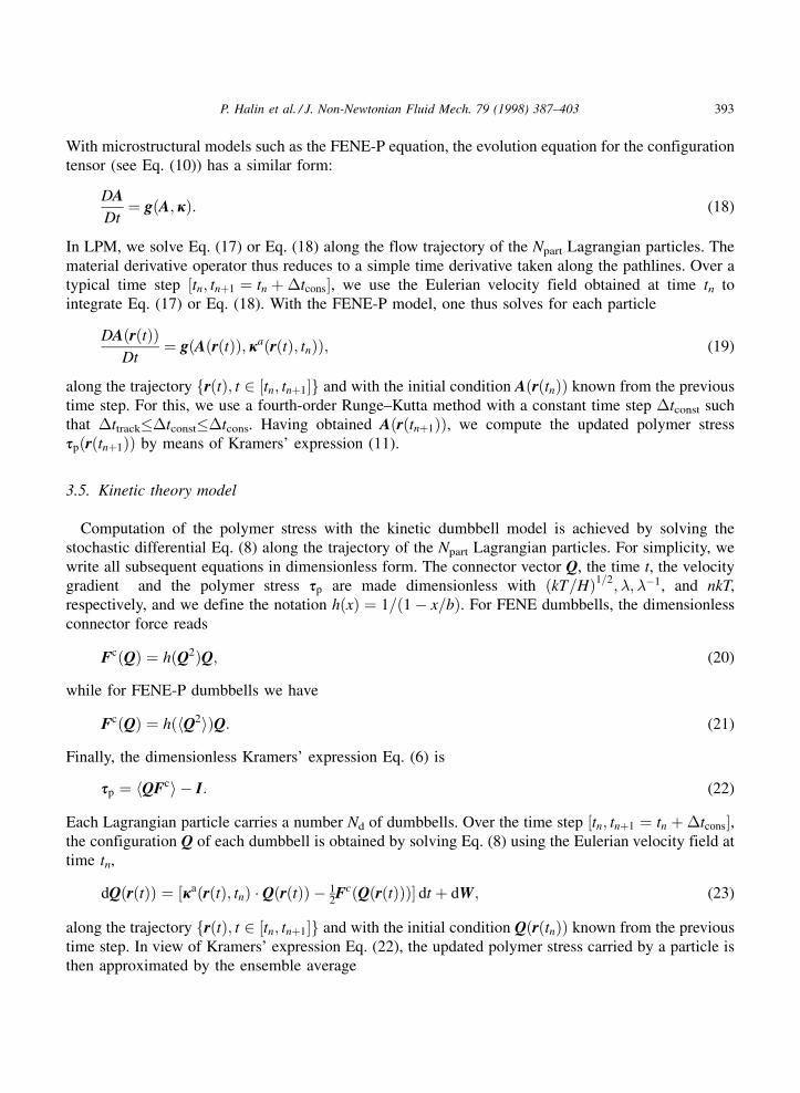
The effect of variance reduction brought about by the use of correlated ensembles of dumbbells ismuch more dramatic in Fig. 5. Here, we present the results of nine independent LPM simulations usingonly Nd � 450 dumbbells in each Lagrangian particle. The fluctuations in the stress and velocity aremuch reduced with correlated ensembles of dumbbells. One should note, however, that the polymerstress results obtained with correlated ensembles, though much smoother, do vary a lot from one run tothe other. In addition, the average over the nine independent runs is less accurate than that computedwith uncorrelated ensembles. A plausible explanation is that, with such a small number of dumbbells ineach particle, the use of correlated ensembles does not allow for an accurate generation of the initialequilibrium distribution.

Stochastic micro±macro simulations are mainly limited by the availability of computer memory.Using a fixed set of numerical parameters, including Npart and Nd, it may be practically feasible toaverage the results of a number NR of independent LPM realizations, while a single run with NR times

Fig. 3. Temporal evolution of velocity and polymer stress in the region of thinnest gap (see Fig. 2) obtained with the FENE-P

constitutive equation. The Newtonian velocity is shown for reference. Results of the macroscopic and micro±macro LPM

simulations are in excellent agreement with those obtained by means of the mixed finite element method (Eulerian macro).

P. Halin et al. / J. Non-Newtonian Fluid Mech. 79 (1998) 387±403 397

more dumbbells in each particle would not fit the available memory. In view of the non-linear couplingbetween polymer stress and velocity, it is not obvious that this simple averaging procedure behavessatisfactorily. Fig. 6 provides a positive answer in that regard, at least for the flow problem consideredhere.

Let R�i��t� denote the result of the ith stochastic LPM run at time t. We take the correspondingmacroscopic LPM result Rmacro(t) as a reference solution. Using a number nr of independent results(1� nr � NR), one obtains the average

R�nr�av �t� �

1

nr

Xnr

i�1

R�i��t�: (28)

Fig. 4. Temporal evolution of velocity and polymer stress in the region of thinnest gap (see Fig. 2) obtained with the FENE-P

constitutive equation. Three individual micro±macro LPM simulation results, obtained with correlated or uncorrelated

ensembles of 4500 dumbbells in each Lagrangian particle, are compared to their macroscopic LPM counterparts. The average

of the three individual micro-macro results is also shown.

398 P. Halin et al. / J. Non-Newtonian Fluid Mech. 79 (1998) 387±403

An estimate of the numerical error carried by this average is given by the mean quadratic error

e�nr� � 1

tf ÿ t0

Z tf

t0

�R�nr�av �t� ÿ Rmacro�t��2dt; (29)

where the relevant time interval [t0, tf] is set to [0, 15] in the present case (cfr. Fig. 4). Since we have atotal of NR independent LPM results at our disposal, there are N�nr� � NR!=nr!�NRÿ nr�! ways offorming the average Eq. (28), each carrying a mean quadratic error Eq. (29). It is the average of theseerrors, computed over the N(nr) possible combinations, that is plotted in Fig. 6 as a function of nr. Here,the result R being considered is either the velocity or the polymer stress. The evolution of the average

Fig. 5. Temporal evolution of velocity and polymer stress in the region of thinnest gap (see Fig. 2) obtained with the FENE-P

constitutive equation. Nine individual micro±macro LPM simulation results, obtained with correlated or uncorrelated

ensembles of 450 dumbbells in each Lagrangian particle, are compared to their macroscopic LPM counterparts. The average

of the nine individual micro±macro results is also shown.

P. Halin et al. / J. Non-Newtonian Fluid Mech. 79 (1998) 387±403 399

error is indeed consistent with the 1=�����nrp

behavior that would be obtained without the stress±velocitycoupling.

4.4. Micro±macro LPM computations with FENE dumbbells

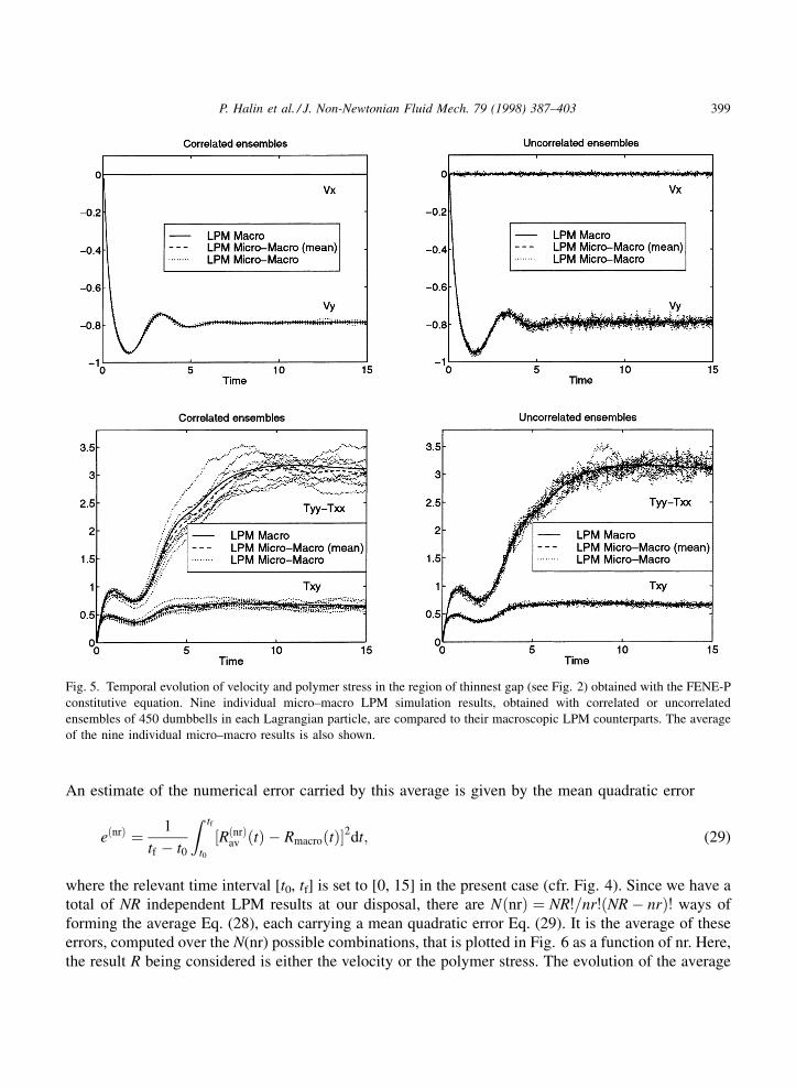
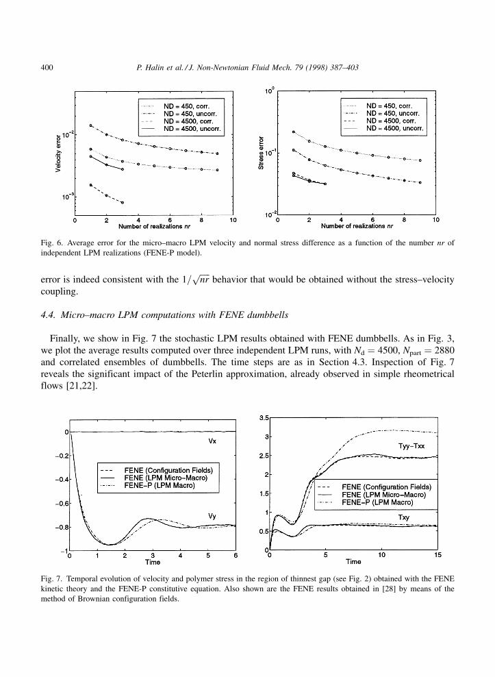
Finally, we show in Fig. 7 the stochastic LPM results obtained with FENE dumbbells. As in Fig. 3,we plot the average results computed over three independent LPM runs, with Nd � 4500, Npart � 2880and correlated ensembles of dumbbells. The time steps are as in Section 4.3. Inspection of Fig. 7reveals the significant impact of the Peterlin approximation, already observed in simple rheometricalflows [21,22].

Fig. 6. Average error for the micro±macro LPM velocity and normal stress difference as a function of the number nr of

independent LPM realizations (FENE-P model).

Fig. 7. Temporal evolution of velocity and polymer stress in the region of thinnest gap (see Fig. 2) obtained with the FENE

kinetic theory and the FENE-P constitutive equation. Also shown are the FENE results obtained in [28] by means of the

method of Brownian configuration fields.

400 P. Halin et al. / J. Non-Newtonian Fluid Mech. 79 (1998) 387±403

We also show in Fig. 7 the results obtained by our T.U. Delft colleagues [28] for the same flowproblem, using their Brownian configuration fields approach [11]. The agreement with the LPM resultsis very good indeed.

5. Discussion and conclusions

The above results demonstrate the ability of LPM to produce accurate numerical results in a non-trivial time-dependent viscoelastic flow problem, using either a macroscopic constitutive equation ofthe differential type or a kinetic theory model for the polymer dynamics.

Table 2 summarizes the computer resources (CPU time and main memory capacity) needed forobtaining the results illustrated in Figs. 3±5 for FENE-P dumbbells with the 4�80 finite element mesh.The particular computer used in this work is a SGI Indigo2 R10000 workstation.

We wish to point out that the data in Table 2 for the Eulerian macroscopic simulation are only shownfor the sake of completeness, and are not representative of the state-of-the-art of Eulerian methods fortransient viscoelastic flows. Indeed, the implicit mixed method implemented by Purnode and Crochet[26] was not designed with transient flows in mind as it solves at each time step the full set ofdiscretized equations by means of a Newton scheme, which of course is rather expensive. At any rate,the macroscopic LPM approach is quite attractive in terms of computer resources. Another strong pointof the new technique is the stability and accuracy of the Lagrangian integration of the constitutiveequation along the particle paths. Indeed, LPM takes account in a most natural way of the purelyconvective nature of differential viscoelastic constitutive equations.

The micro±macro LPM runs, with either correlated or uncorrelated ensembles of dumbbells, aresignificantly more expensive than macroscopic computations, but they remain feasible on availablehardware. This is of course the price to pay for the direct use in flow simulation of kinetic theorymodels, such as the FENE dumbbell model, which cannot be translated into an equivalent macroscopicconstitutive equation. Use of correlated ensembles of dumbbells not only reduces the statistical noiseaffecting the results but also does decrease the CPU time by almost a factor of two in the present case.One should also note that tracking the motion of the Lagrangian particles and the expensive task ofevaluating the particle polymer stress can be implemented on parallel computers using algorithmssimilar to those already developed for integral constitutive equations [29±31].

A number of numerical issues related to LPM still deserves further investigation. In particular,theoretical developments are needed to better understand the transfer of information between theLagrangian stress calculation and the Eulerian conservation equations, and the smoothing effect thatthis transfer may have. In this work, we used successfully a piecewise discontinuous least-squares

Table 2

Computer resources for the FENE-P simulations of Figs. 3±5, with �tcons � 10ÿ2 and [t0, tf] � [0,15]

Method Npart Nd CPU (s) Memory (MB)

Eulerian macro ± ± 62 285 81

LPM macro 2880 ± 2 607 16

LPM micro±macro (correlated ensembles) 2880 4500 94 900 313

LPM micro±macro (uncorrelated ensembles) 2880 4500 165 791 313

P. Halin et al. / J. Non-Newtonian Fluid Mech. 79 (1998) 387±403 401

interpolation of the Lagrangian polymer stress values. Use of continous least-squares interpolationproduced numerical instabilities [25] for reasons which remain to be understood. The numericalimplications of using correlated ensembles of dumbbells with LPM also deserve further study. Asdemonstrated in the present work, LPM can also be used with uncorrelated ensembles of dumbbells forproblems where the physical fluctuations become relevant [24]. Finally, criteria remain to be developedfor selecting optimal values of the numerical parameters (number of Lagrangian particles, number ofdumbbells, and the various time steps) for a given flow problem and its spatial discretization.

The major next step in the development of LPM is the design of an adaptive algorithm that wouldallow the automatic creation or deletion of Lagrangian particles when and where needed, in order tomeet specific accuracy requirements. Other useful extensions of LPM include the use of integralconstitutive equations and their related stochastic formulations [32,33], the implementation ofcapabilities for free-surface flows, and porting to parallel computer. We plan to report on thesedevelopments in the near future.

Acknowledgements

This work is supported by the ARC 97/02-210 project, Communaute Franc,aise de Belgique, and theBRITE/EURAM project MPFLOW CT96-0145. The work of V. Legat is supported by the BelgianFonds National de la Recherche Scientifique (FNRS). We thank our T.U. Delft colleagues MartienHulsen and Ben van den Brule for helpful discussions and for sharing with us their unpublished results[28].

References

[1] M.J. Crochet, A.R. Davies, K. Walters, Numerical Simulation of Non-Newtonian Flow, Elsevier, Amsterdam, 1984.

[2] M.J. Crochet, Simulation of viscoelastic flow. Rubber Chemistry and Technology, Am. Chem. Soc. 62 (1989) 426±455.

[3] R. Keunings, Simulation of viscoelastic fluid flow, in: C.L. Tucker III, (Ed.), Fundamentals of Computer Modeling for

Polymer Processing, Hanser, Munich, 1989, pp. 402±470.

[4] R. Keunings, P. Halin, Macroscopic and mesoscale approaches to the computer simulation of viscoelastic flows in:

J.R.A. Pearson, M.J. Adams, R.A. Mashelkar, A.R. Rennie (Eds.), Dynamics of Complex fluids, Imperial College Press,

The Royal Society, 1998, in press.

[5] F.P.T. Baaijens, Mixed finite element methods for viscoelastic flow analysis: a review, J. Non-Newtonian Fluid Mech.,

1998, this volume.

[6] H.C. OÈ ttinger, M. Laso, `Smart' polymers in finite-element calculations, in: P. Moldenaers, R. Keunings, (Eds.), Proc.

10th Int. Congr. on Rheology, Elsevier, Amsterdam, 1992, pp. 286±288.

[7] M. Laso, H.C. OÈ ttinger, Calculation of viscoelastic flow using molecular models: the CONNFFESSIT approach, J. Non-

Newtonian Fluid Mech. 47 (1993) 1±20.

[8] K. Feigl, M. Laso, H.C. OÈ ttinger, The CONNFFESSIT approach for solving a two-dimensional viscoelastic fluid

problem, Macromolecules 28 (1995) 3261±3274.

[9] C.C. Hua, J.D. Schieber, Application of kinetic theory models in spatiotemporal flows for polymer solutions, liquid

crystals and polymer melts using the CONNFFESSIT approach, Chem. Eng. Sci. 51 (1996) 1473±1485.

[10] M. Laso, M. Picasso, H.C. OÈ ttinger, 2D time-dependent viscoelastic flow calculations using CONNFFESSIT, AIChE J.

43 (1997) 877±892.

[11] M.A. Hulsen, A.P.G. van Heel, B.H.A.A. van den Brule, Simulation of vicoelastic flows using Brownian configuration

fields, J. Non-Newtonian Fluid Mech. 70 (1997) 79±101.

402 P. Halin et al. / J. Non-Newtonian Fluid Mech. 79 (1998) 387±403

[12] T.W. Bell, G.H. Nyland, J.J. de Pablo, M.D. Graham, Combined Brownian dynamics and spectral simulation of the

recovery of polymeric fluids after shear flow, Macromolecules 30 (1997) 1806±1812.

[13] R.B. Bird, C.F. Curtiss, R.C. Armstrong, O. Hassager, Dynamics of Polymeric Liquids, Kinetic theory, 2nd ed., vol. 2,

Wiley-Interscience, New York, 1987.

[14] R.B. Bird, R.C. Armstrong, O. Hassager, Dynamics of Polymeric Liquids, Fluid mechanics, 2nd ed., vol. 1, Wiley-

Interscience, New York, 1987.

[15] R.G. Larson, T.T. Perkins, D.E. Smith, S. Chu, Hydrodynamics of a DNA molecule in a flow field, Phys. Rev. E 55/2

(1997) 1794±1797.

[16] M.R.J. Verhoef, B.H.A.A. van den Brule, M.A. Hulsen, On the modelling of a PIB/PB Boger fluid in extensional flow. J.

Non-Newtonian Fluid Mech., 1998, submitted for publication.

[17] G. Lielens, P. Halin, I. Jaumain, R. Keunings, V. Legat, New closure approximations for the kinetic theory of finitely

extensible dumbbells, J. Non-Newtonian Fluid Mech. 76 (1998) 249±279.

[18] R. Sizaire, G. Lielens, I. Jaumain, R. Keunings, V. Legat, On the hysteretic behaviour of dilute polymer solutions in

relaxation following extensional flow, J. Non-Newtonian Fluid Mech., May 1998, in press.

[19] P.S. Doyle, E.S.G. Shaqfeh, G.H. McKinley, S.H. Spiegelberg, Relaxation of dilute polymer solutions following

extensional flow, J. Non-Newtonian Fluid Mech. 76 (1998) 79±110.

[20] H.C. OÈ ttinger, Stochastic Processes in Polymeric Fluids: Tools and Examples for Developing Simulation Algorithms,

Springer, Berlin, 1996.

[21] M. Herrchen, H.C. OÈ ttinger, A detailed comparison of various FENE dumbbell models, J. Non-Newtonian Fluid Mech.

68 (1997) 17±42.

[22] R. Keunings, On the Peterlin approximation for finitely extensible dumbbells, J. Non-Newtonian Fluid Mech. 68 (1997)

85±100.

[23] A. Goublomme, B. Draily, M.J. Crochet, Numerical prediction of extrudate swell of a high-density polyethylene, J. Non-

Newtonian Fluid Mech. 44 (1992) 171±195.

[24] H.C. OÈ ttinger, B.H.A.A. van den Brule, M.A. Hulsen, Brownian configuration fields and variance reduced

CONNFFESSIT, J. Non-Newtonian Fluid Mech. 70 (1997) 255±261.

[25] P. Halin, Ph.D. Thesis, Universite catholique de Louvain, Belgium, in preparation.

[26] B. Purnode, M.J. Crochet, Flows of polymer solutions through contractions. Part 1. Flow of polyacrylamide solutions

through planar contractions, J. Non-Newtonian Fluid Mech. 65 (1996) 269±289.

[27] P. Halin, R. Keunings, M. Laso, H.C. OÈ ttinger, M. Picasso, Evaluation of a micro-macro computational technique in

complex polymer flows, in: A. Ait-Kadi et al., (Eds.), Proc. 12th Int. Cong. on Rheology, 1996, pp. 401±402.

[28] W.J. ter Horst, Simulation of a viscoelastic flow in a journal bearing geometry using Brownian configuration fields.

Technical Report, Msc internal report MEAH-172, Laboratory for Aero and Hydrodynamics, Delft University of

Technology, January 1998.

[29] R. Aggarwal, R. Keunings, F.-X. Roux, Simulation of the flow of integral viscoelastic fluids on a distributed memory

parallel computer, J. Rheol. 38(2) (1994) 405±419.

[30] P. Henriksen, R. Keunings, Parallel computation of the flow of integral viscoelastic fluids on a heterogeneous network of

workstations, Int. J. Numer. Meth. Fluids 18 (1994) 1167±1183.

[31] R. Keunings, Parallel finite element algorithms applied to computational rheology, Computers Chem. Eng. 19(6/7)

(1995) 64±669.

[32] K. Feigl, H.C. OÈ ttinger, A new class of stochastic simulation models for polymer stress calculation, J. Chem. Phys. 109

(1998) 815±826.

[33] K. Feigl, H.C. OÈ ttinger, Towards realistic rheological models for polymer melt processing, Macromol. Symp. 121 (1997)

187±203.

P. Halin et al. / J. Non-Newtonian Fluid Mech. 79 (1998) 387±403 403