The Labor Market Impact of Undocumented Immigrants: Job ...

The Labor Market Impact of Undocumented Immigrants:Job Creation vs. Job Competition∗

Christoph Albert†

Universitat Pompeu Fabra

April 3, 2017

Abstract

This paper presents novel evidence on the effect of legal status on workers’ labor marketoutcomes in the US and explores the impact of undocumented immigration in a labormarket model featuring search frictions and non-random hiring. Firms receive applica-tions from documented and undocumented workers and hire the worker they can extractthe largest surplus from. As undocumented workers have a lower reservation wage dueto their ineligibility for unemployment benefits, lower wage bargaining power and risk ofbeing detected and removed, their wages are lower and job finding rates higher, which isconsistent with the empirical evidence. An increase in the share of undocumented immi-grants leads to the creation of additional jobs, but also more competition for documentedjob seekers. When calibrated to US data, the job creation effect dominates and undocu-mented immigration benefits documented workers. An increase in the removal rate mutesjob creation and thus lowers the job finding rate of all workers. This detrimental effect iseven larger if the removal rate increases more for employed workers (e.g. through worksiteraids) because this leads to a risk premium in their wages. Using the introduction of state-wide omnibus immigration laws as a measure of increased removal risk, I find evidence formuted job creation and a risk premium in immigrants’ wages.

Keywords: wage gap, migrant workers, hiring, employment.

JEL: J31, J61, J63, J64.

∗This is a preliminary draft of work in progress. I thank my advisors Regis Barnichon and Albrecht Glitz fortheir guidance and encouragement throughout the project. I am also grateful to Joan Monras, Jordi Galí, JanStuhler, Jesús Fernández-Huertas Moraga and participants of the CREI Macroeconomics Breakfast, the CREIInternational Lunch, the CEMFI PhD workshop, the BGSE PhD Jamboree 2016, the CEUS Workshop 2016and the SMYE 2017 for their helpful comments and suggestions.†Universitat Pompeu Fabra, Department of Economics and Business, Carrer Ramon Trias Fargas, 25-27

08005 Barcelona; e-mail: [email protected]

1

1 Introduction

Is immigration beneficial for native workers because it leads to the creation of additional jobs

or does it harm their labor market prospects through higher job competition? This question

has been the subject of much debate as many developed countries saw rising immigrant inflows

throughout the last few decades. In the United States, the share of foreign-born residents

among the population has increased from around 5% in the 1970’s to over 13% today, triggered

by a change in immigration policy during the 1960s facilitating entry from Latin America and

Asia and causing a shift in the skill composition towards less educated immigrants. A second

major shift in the nature of US immigration especially since the beginning of the 1990s is un-

documented immigration. While the number of all immigrants residing in the US doubled from

around 20 million to 40 million between 1990 and 2013, the number of immigrants without

legal status increased almost fourfold from 3 million to over 11 million during the same period.1

Undocumented immigrants in the US actively participate in labor market, constituting around

5% of the labor force.2

The goal of this paper is to shed new light on the labor market impact of undocumented im-

migration and on the question whether stricter immigration enforcement protects documented

workers. I first present novel evidence on the effect of documentation status on workers’ labor

market outcomes and then analyze the effects of undocumented immigration in a labor market

model featuring search frictions and non-random hiring consistent with the empirical findings.

In this framework, the immigration of undocumented workers leads to increased job creation

but also poses higher job competition for documented workers. These effects are both induced

by lower reservation wages of undocumented workers and have opposing effects on the employ-

ment of documented workers. Calibrated to US data, the model suggests that undocumented

immigration is beneficial for documented workers because of a dominating job creation effect.1There exist divergent figures of the number of undocumented immigrants in the US depending on the

estimation method. The cited numbers are taken from the Pew Research Center, whose estimation relies on a"residual method". This method is based on a census count or survey estimate of the number of foreign-bornresidents who have not become U.S. citizens and subtracts estimated numbers of legally present individuals invarious categories from administrative data. The resulting residual is an indirect estimate of the size of theundocumented immigrant population.

2Borjas (2016) for example finds that among the male population, the employment rate of undocumentedimmigrants is higher than both the employment rate of natives and legal immigrants.

2

Stricter immigration enforcement that leads to a higher deportation (or "removal") probability

mutes job creation, even more so if this policy targets rather employed than unemployed un-

documented workers.

My first contribution to the literature consists in showing that documentation status is an

important driver of labor market outcome differences across workers. In particular, I find that

undocumented immigrants earn lower wages and have higher job finding rate than both natives

and documented immigrants. Although the latter earn less and find jobs faster than natives

as well, the differences are smaller and almost disappear for immigrants that have spent more

than 25 years in the US. Having spent fewer years in the US is also associated with lower

earnings and a higher job finding rate (for both types of immigrants). These findings suggest a

connection between low wages and high job finding rates and are to the best of my knowledge

novel in the literature. The second contribution is the analysis of the impact of undocumented

immigration in a search and matching model featuring non-random hiring that is consistent

with the empirical facts. I assume that workers are either documented or undocumented and

that the latter have a lower reservation wage than the former. This explains the wage gap

between the two worker types. While a difference in wages between otherwise identical workers

can also be generated in a standard job search model, the difference in job finding rates is a

puzzle for a model with random matching between firms and workers. I therefore include a

non-random hiring mechanism (following Barnichon and Zylberberg, 2014) in my framework,

which implies that firms can receive multiple applications and choose their preferred candidate

among them (Barron et al. 1985, Barron and Bishop 1985). This generates higher job finding

probabilities and employment rates for cheaper workers as suggested by the data.

The key characteristics implying a lower reservation wage for undocumented workers are in-

eligibility for unemployment benefits, a lower wage bargaining power and a risk of removal,

whereby most of the reservation wage gap is driven by the bargaining power difference. Due

to this gap, firms make a higher surplus by hiring undocumented job seekers and an increase

in their share in the unemployed pool has two opposing effects: The job creation effect, which

is the only effect present in the standard framework, induces firms to create more vacancies

as expected wage costs fall and therefore leads to higher wages and job finding rates for all

3

workers. The competition effect on the other hand, which is only present once we allow for

non-random hiring, lowers documented workers’ job finding as there is a higher probability

of competing with an undocumented applicant. Which of the two effects dominates depends

on the size of the reservation wage difference between the worker types. The higher are the

wage costs that firms can save by hiring an undocumented instead of a documented worker,

the stronger is the job creation effect and the more beneficial is undocumented immigration.

After calibrating the model to match the data, I simulate an increase in the population share

of undocumented immigrants and find that the job creation effect dominates the competition

effect because the wage difference is large enough and expected wage costs of firms fall strongly.

Hence, undocumented immigration is unambiguously beneficial for documented workers as it

raises their job finding rates and wages.

Finally, I use the framework to simulate a policy of stricter immigration enforcement by in-

creasing the removal risk. One effect of this is an increase in the break-up probability for

matches with undocumented workers, which lowers job creation and depresses job finding rates

and wages of all workers. A second effect arises, if the risk increases more strongly for employed

than for unemployed undocumented workers. A higher removal rate for the employed implies

that firms have to pay a risk compensation in order to induce an undocumented worker to

accept a job. This compensation raises expected wage costs, decreases the expected profits

from opening a vacancy and as a consequence depresses job creation and job finding rates of all

workers further. This second effect is larger, the higher is the disutility associated with removal.

Testing the model’s predictions using the state-wide implementation of omnibus immigration

laws as a measure of increased removal risk, I find that these laws are associated with a lower

job finding rate for all workers, which is evidence for muted vacancy creation. Moreover, I find

that they are associated with lower wages for natives and higher wages for immigrants, which

is consistent with a risk compensation in immigrants’ wages.

Previous studies on migration in the US often only considered the distinct skill composition or

experience profiles of immigrants in their models (e.g. Borjas, 2003, Peri and Sparber, 2009, Ot-

taviano and Peri, 2012, Llull, 2013). However, as being undocumented is highly correlated with

skills (on average undocumented immigrants have a lower education than documented ones) le-

4

gal status as an additional dimension of immigrant heterogeneity should not be neglected.3 An

exception is a study by Edwards and Ortega (2016) who differentiate between documented and

undocumented immigrants. Contrary to my framework, the authors assume a frictionless labor

market with wages equal to marginal productivity, which implies that the earnings differences

between documented and undocumented workers are solely due to productivity differences.

This is a questionable assumption as there are various other explanations for lower earnings

of undocumented workers that are not related to productivity. Since the undocumented are

not legally permitted to work, firms are not bound to any minimum wage laws and might use

the threat of being sanctioned for hiring them to justify paying lower wages. Furthermore, the

inability to receive unemployment benefits lowers the outside option to working and suppresses

the wages of undocumented workers additionally. I therefore use a framework with search fric-

tions that easily allows to consider these points by assuming differences in bargaining power

and unemployment benefits across worker types. Other closely related work employing a model

with search frictions to study employment and wage effects of immigration is by Chassamboulli

and Peri (2015). They assume that all workers are equally productive but that immigrants, and

even more so the subgroup of the undocumented, have lower reservation wages than natives.

The prospect of hiring workers at a lower cost increases firms’ profit and induces job creation,

a mechanism also at work in this paper. However, their search model features random hiring,

i.e. although firms can discriminate between natives and immigrants once they are matched,

they cannot do so in their hiring. Hence, all workers always have the same job finding rate and

therefore immigration unambiguously drives up wages and employment of natives. As I find

that the prediction of equal job finding rates across worker types is not supported by the data,

I tackle the assumption of random hiring in this paper.

The fact that many immigration studies stress the different skill distribution of immigrants

and consider natives and immigrants as imperfect substitutes raises the question whether the

assumption of perfect substitutability between natives, documented and undocumented im-

migrants made throughout the paper is too strong. To address this concern, I filter out skill

differences as thorough as possible in my empirical investigation, which is why all results should3Of course, most studies do not distinguish immigrants by legal status simply because an identifier to do so

was not available. A reliable method to identify undocumented immigrants has just become recently available(see section 2.1).

5

be viewed as being conditional on having the same skills. In particular, I only focus on low-

skilled workers and add an extensive set of demographic, occupation and industry controls in

the regressions, including an interaction between industry and occupation fixed effects. Thus,

I assume that natives, legal and undocumented immigrants are perfect substitutes only within

each narrowly defined industry-occupation cell. I thereby control for imperfect substitutability

within broader skill cells as emphasized by previous studies. This allows me to uncover doc-

umentation status as an additional and so far neglected dimension of heterogeneity. In that

sense, my work complements the literature focussing on skill heterogeneity.

The remainder of the paper is organized as follows. In section 2, I describe how undocumented

immigrants are identified in the data and present some descriptive statistics. Section 3 analyzes

wages and job finding rates of natives, documented and undocumented immigrants empirically.

Section 4 sets up the search model with non-random hiring. Section 5 outlines the calibration

strategy. Section 6 examines the effect of undocumented immigration of workers in the cali-

brated model. Section 7 explores the impact of a change in the removal risk. Section 8 tests

some predictions derived from the model empirically. Section 9 concludes.

2 Data, Identification Method and Descriptives

In the following section, I describe the data and the method of identifying undocumented

immigrants used. This method is first described in Borjas (2016) and based on demographic,

social and economic characteristics of survey respondents. I show that the percentage of both

documented and undocumented immigrants is by far the highest among workers without a high

school degree. I further highlight the demographic differences between natives and immigrants

and their concentration across industries by education level.

2.1 Data and Identification of Undocumented Immigrants

The data used in this section come from the March supplement of the Current Population

Survey (CPS) obtained from IPUMS. My analysis is restricted to the period beginning in 1994

because information on the birthplace and citizenship status of a survey respondent was only

included from that year on. I only include prime age workers (age 25 to 65) in all samples. A

6

respondent is defined as an immigrant, if he is born outside the United States and not American

citizen by birth. In section 3.2, I further use the basic monthly files of the CPS with workers

matched over two consecutive months following Shimer (2012) in order to examine transition

rates between employment and unemployment.

Neither the CPS basic monthly files nor the March supplement allow to directly identify undoc-

umented immigrants. However, as the US labor market surveys are address-based and designed

to be representative of the whole population, they also include undocumented respondents. The

CPS data are likely to offer the best coverage of undocumented immigrants because individuals

are interviewed in person, whereas for the US Census and ACS data are collected by mail.4 The

government surveys are actually used by the US Department of Homeland Security (DHS) to

estimate the size of the undocumented immigrant population via a so-called "residual method".

The DHS obtains the number of legal immigrants in the US from administrative data of of-

ficially admitted individuals and subtracts them from the foreign-born non-citizen population

estimated from the surveys. The resulting residual is the estimated number of unauthorized

residents.

Recently, a methodology for identifying undocumented immigrants at the individual level in

the survey data was developed by Passel and Cohn (2014). They add an undocumented status

identifier based on respondents’ demographic, social, economic and geographic characteristics

to the CPS March supplement. They use variables like citizenship status or coverage by public

health insurance to identify a foreign-born respondent as legal and then classify the remaining

immigrants as "potentially undocumented". As a final step, they apply a filter on the poten-

tially undocumented immigrants to ensure that the count of the immigrants that are finally

classified as undocumented is consistent with the estimates from the residual method. Unfortu-

nately, their code is not available for replication. However, Borjas (2016) describes a simplified

and replicable version of the methodology of Passel and Cohn (2014) based on the 2012-2013

CPS files they constructed, which he uses to identify undocumented respondents in all CPS

March supplements since 1994. I follow his algorithm and replicate the undocumented status4Only one third of those who do not respond to the ACS survey initially are randomly selected for in-person

interviews, which could result in an underrepresentation of undocumented respondents, who might ignore thesurvey due to the fear of detection.

7

identifier in the CPS March supplement data. Borjas (2016) does not apply a filter to take

care of the overcounting of undocumented immigrants in the microdata as the DHS residual

method does but shows that his method yields an undocumented immigration population that

is similar in terms of size and demographic characteristics to the one in Passel and Cohn (2014).

Borjas’ simplified identification method consists in classifying every immigrant who does not

fulfill at least one of the following condition as undocumented:

• being US citizen

• residing in the US since 1980 or before

• receiving social security benefits or public health insurance

• residing in public housing or receiving rental subsidies

• being veteran or currently in the Armed Forces

• working in the government sector or in occupations requiring licensing

• being Cuban

• married to a legal immigrant or US citizen

Figure 1 plots the share of undocumented immigrants identified with the method of Borjas

(2016) among the total prime age population and among all prime age immigrants since 1994

in the four groups commonly used for the classification of educational attainment: high school

dropouts, high school graduates, workers with some college education and college graduates.

Among high school dropouts, the percentage of undocumented immigrants is by far the highest

and increased the strongest, from 7% in 1994 to almost 25% in 2015. In the higher education

groups, the percentage has risen only moderately, reaching just above 5% for high school and

college graduates.5 Also among immigrants, the percentage of undocumented is the largest and5A part of the rise of the undocumented share among high school dropouts is due to the fact that education

levels of natives and documented immigrants have improved more strongly than education levels of undocu-mented immigrants (between 1994 and 2016 the share of high school dropouts has fallen from 15% to 9% forthe former and from 41% to 37% for the latter).

8

Figure 1: Percentage of undocumented immigrants

% of total population % of all immigrants

05

10

15

20

25

Undocum

ente

d (

%)

1994 1996 1998 2000 2002 2004 2006 2008 2010 2012 2014 2016Year

< HS HS

Some College College

010

20

30

40

50

Undocum

ente

d (

%)

1994 1996 1998 2000 2002 2004 2006 2008 2010 2012 2014 2016Year

< HS HS


Source: CPS March supplement with Borjas (2016) identification, prime age workers only

increased the most in the group of high school dropouts. This suggests that on average undoc-

umented have a lower education than documented immigrants and this difference is increasing

over time (the percentage of high school dropouts is around 37% among the former and 19%

among the latter in 2016).

Table 1 shows some descriptive statistics of the sample of prime age workers covering the most

recent ten years (2007-2016) by education and status (native, documented immigrant or undoc-

umented immigrant). Across all education levels, undocumented workers are six to seven years

younger than both native and documented workers, who have around the same age. More-

over, depending on the education level, documented are 9 to 13 years longer in the US than

undocumented immigrants. However, this is partially because all immigrants that reside in

the US since 1980 or before are classified as legal.6 Irrespective of education, the percentage

of men among documented immigrants is somewhat lower and among undocumented some-

what higher than among natives. The shares of hispanic and asian workers differ substantially

across the level of education education. Among undocumented high-school dropouts, 89% of

workers are hispanic and this percentage decreases strongly with education. Among college6This is due to the Immigration Reform and Control Act of 1986 (IRCA), which granted amnesty to all

undocumented immigrants that had entered the US in 1980 or before.

9

Table 1: Descriptive statistics

Education Status Age Years in US % Men % Hispanic % AsianNative 45 - 52 23 3

<HS Doc. 45 21 48 77 13Undoc. 39 12 57 89 7Native 45 - 50 11 2

HS Doc. 44 21 46 49 23Undoc. 38 11 54 69 15Native 44 - 45 10 3

SC Doc. 44 22 44 37 25Undoc. 38 11 51 51 19Native 44 - 46 5 4

C Doc. 44 20 45 18 44Undoc. 37 7 53 18 57

Note: The statistics are averages across the 2007-2016 CPS March supplement and drawn from the prime ageworker sample described in the text.

graduates without documentation only 18% are of hispanic origin. A similar pattern holds for

documented immigrants, although their share of hispanic workers is lower than among undocu-

mented immigrants. For the the share of asian workers, we observe the opposite pattern across

education levels: the higher is education, the higher is the share of asians among immigrants.

Moreover, for workers with less than a college degree there are more asians among documented

than among undocumented immigrants.

Figure 2 explores whether worker status is associated with a concentration in different in-

dustries. I identify 13 different industries based on the one-digit level of the North American

Industry Classification System (NAICS). The most salient feature of the figure is the high num-

ber of both documented and undocumented immigrant workers among high school dropouts,

which is in most industries close to the number of native workers. Only Wholesale and Retail

Trade, Transportation and Utilities, Education and Health as well as Government7 are largely

dominated by a native workforce. In Agriculture, native workers are even a small minority

among workers without high school degree. Most undocumented high school dropouts work7By construction of the identification method, no undocumented immigrants work for the government.

10

Figure 2: Worker distribution across industries by education0

.2.4

.6W

ork

ers

(m

illio

n)

Agricultu

re

Mining

Constructi

on

Manufacturin

g

Wholesa

le/Retail T

rade

Transp

ortatio

n/Utili

ties

Informatio

n

Finance

Prof./B

usiness

Servi

ces

Educatio

n/Health

Leisure

/Hosp

itality

Other Servi

ces

Govern

ment

< High school

Native Documented Undocumented

01

23

4W

ork

ers

(m

illio

n)

Agricultu

re

Mining

Constructi

on

Manufacturin

g

Wholesa

le/Retail T

rade

Transp

ortatio

n/Utili

ties

Informatio

n

Finance

Prof./B

usiness

Servi

ces

Educatio

n/Health

Leisure

/Hosp

itality

Other Servi

ces

Govern

ment

High school


01

23

45

Work

ers

(m

illio

n)

Agricultu

re

Mining

Constructi

on

Manufacturin

g

Wholesa

le/Retail T

rade

Transp

ortatio

n/Utili

ties

Informatio

n

Finance

Prof./B

usiness

Servi

ces

Educatio

n/Health

Leisure

/Hosp

itality

Other Servi

ces

Govern

ment

Some college


02

46

810

Work

ers

(m

illio

n)

Agricultu

re

Mining

Constructi

on

Manufacturin

g

Wholesa

le/Retail T

rade

Transp

ortatio

n/Utili

ties

Informatio

n

Finance

Prof./B

usiness

Servi

ces

Educatio

n/Health

Leisure

/Hosp

itality

Other Servi

ces

Govern

ment

College



in the Construction and Leisure and Hospitality industry. In the latter, which includes for

example cooks and waiters, they constitute even the largest share of the three worker types.

The upper right and bottom panels suggest that among higher educated workers with at least

a high school degree, the number of immigrants is small compared to the number of natives

across all industries. Furthermore, the number of undocumented is always smaller than the

number of documented immigrants.

Given the large size of the immigrant workforce relative to natives among high school dropouts,

I choose to restrict my empirical analysis to this education level only (for simplicity henceforth

referred to as "low-skilled"). Beside the large share of both documented and undocumented

immigrant workers, there are three more reasons for focusing on this group. First, the identi-

11

fication method is more precise among low-skilled workers because some of the variables used

for identification like receiving social security benefits are less relevant for the high-skilled. In

the Appendix I provide a back-of-the-envelope calculation of the percentage of correctly iden-

tified undocumented immigrants in each education group, which I find to be around 100% for

low-skilled and only around 40%-50% for college educated workers. Second, concentrating on

workers that are homogenous in terms of their education level is likely to lead to a more precise

estimation of the effect of legal status. Third, unobserved skill differences between natives,

documented and undocumented immigrants play a rather small role in the low-skilled labor

market.8

3 Empirical Evidence

Next, I present empirical evidence supporting the claim that the labor market performance of

low-skilled workers is not only affected by being an immigrant or a native but depends primarily

on an immigrant’s legal status. In particular, I show that low-skilled undocumented immigrants

earn lower wages than both documented immigrants and natives. A wage gap between the latter

two types is also existent but much smaller in size. The wage gap to natives falls throughout an

immigrant’s stay in the US and disappears completely after 25 years when being documented

but not when being undocumented. Moreover, I find that immigrants find jobs faster than

natives and that, analogously to wages, the gap is higher for undocumented immigrants and for

both types falling in the length of stay in the country. I also find evidence of lower separation

rates of immigrants, although the differences are small and disappear for immigrants that are

more than 25 years in the US. Finally, using a basic Mortensen-Pissarides framework, I show

that the wage and transition rate differences translate to a much lower reservation wage for

undocumented immigrants relative to natives and documented immigrants.

3.1 Wages

It has been well established by the literature that immigrants are paid less than native workers

even when controlling for observables. However, to my knowledge there exists no extensive8All empirical findings in this paper also hold for high school graduates, workers with some college or using

any pooled sample of workers having at most some college education.

12

Figure 3: Hourly wages of low-skilled workers (1999 dollars)

05

10

15

Avera

ge h

ourly w

age

Agricultu

re

Mining

Constructi

on

Manufacturin

g

Wholesa

le/Retail T

rade

Transp

ortatio

n/Utili

ties

Informatio

n

Finance

Prof./B

usiness

Servi

ces

Educatio

n/Health

Leisure

/Hosp

itality

Other Servi

ces

Govern

ment

< High school



empirical research using recent microdata that also takes into account the effect of legal status

on earnings.9 In order to fill this gap in the literature I use the CPS March supplement data

with undocumented immigrants identified by the Borjas (2016) algorithm. Following previous

studies (e.g. Borjas, 2003), I exclude the self-employed, those working without pay, those not

working full-time (52 weeks per year, at least 35 hours per week) and people living in group

quarters.10 I construct real hourly wages by dividing the total wage income of an employee

by the number of hours worked per year, deflating the result to 1999 dollars with the CPI-U

adjustment factor provided in the IPUMS database and controlling for outliers by dropping the

1st and 99th percentile of the distribution of the hourly wage.

Figure 3 reports the average hourly wages of workers without high school degree in each of the

13 industries during the period 2007-2016. Not surprisingly, natives earn the highest wages in

all industries. With the only exception being Mining, documented immigrants have the second9Edwards and Ortega (2016) document wage differences between documented and undocumented immigrants

within industries, but do not perform a more in-depth regression analysis.10Results are robust to keeping part-time workers.

13

highest wages, while undocumented immigrants earn the least. The lowest paying industries

with earnings of under $10 for all types of workers are Leisure and Hospitality, Agriculture and

Education and Health. Except for Mining and Construction, undocumented immigrants earn

hourly wages well below $10 in all industries. However, these figures should be viewed with

caution as Table 1 clearly suggests that the three worker samples differ with respect to demo-

graphic characteristics, which certainly influences their earnings. Controlling for observables

beyond education and industry is therefore crucial.

Figure 4 shows the percentage of workers with hourly earnings below the minimum wage during

the years 2007-2015. I define the minimum wage either as the one in force in the state a worker

is residing in or as the federal minimum wage in case the latter is higher than the former in a

given year. The figure suggests that 35% of undocumented workers working in Agriculture are

paid below the minimum wage. In other industries with a high number of undocumented work-

ers, the percentage lies between 20% and 30%, except in Construction. Pooling all industries,

the percentage of workers earning below minimum wage is around 10 percentage points lower

for documented than for undocumented immigrants and around 4 percentage points lower for

documented immigrants than for natives.

In order to test whether the wage differences between worker types also exist between otherwise

comparable workers, I run a wage regression with an extensive set of demographic controls

including age, age squared, sex, hispanic and asian origin. Additional to demographic factors

and industry fixed effects, I control for the worker’s occupation, which relates to the specific

technical function in a job. Indeed, several studies suggest that natives and immigrants are

imperfect substitutes and tend to specialize in tasks they have a comparative advantage in,

which are more communication-intensive for natives and more manual/physical for immigrants

(Peri and Sparber, 2009, Rica et al., 2013). Thus, additional to industry dummies, I include

a dummy for each of the around 500 occupation codes attributed to a worker in the CPS

data. As a final robustness check, I include an interaction of industry- and occupation-fixed

effects, i.e. a dummy for each industry-occupation combination instead of separate industry and

occupation dummies. By doing so, I assume that only within each industry-occupation cell,

natives, documented and undocumented immigrants are perfect substitutes. The regression

14

Figure 4: Low-skilled workers paid below minimum wage (%)

010

20

30

40

Belo

w m

in. w

age (

%)

Agricultu

re

Mining

Constructi

on

Manufacturin

g

Wholesa

le/Retail T

rade

Transp

ortatio

n/Utili

ties

Informatio

n

Finance

Prof./B

usiness

Servi

ces

Educatio

n/Health

Leisure

/Hosp

itality

Other Servi

ces

Govern

ment

< High school



specification has the following form:

lnwit = β0 + β1Dit + β2Uit + φt +X ′itγ + εit,

where the dummies Dit and Uit are indicators for being a foreign-born documented or undoc-

umented worker, respectively, φt denotes a year-fixed effect and X ′it is a vector containing the

demographic, industry and occupation controls as well as metropolitan-area dummies.

The regression results are reported in Table 2. The baseline specification without controls sug-

gests that documented earn around 12% and undocumented immigrants around 27% less than

the native reference group. The inclusion of demographic controls and metropolitan area and

year fixed effects shrinks the coefficients slightly. The wage differences indicated by column (3)

are in line with the results of a comparable specification in Borjas (2017, Table 2), who finds

very similar coefficients even though he uses a sample with all education groups and only the

years 2012-2013.11 Additionally including industry and occupation fixed effects shrinks both11Borjas (2017) obtains a coefficient of -0.10 for documented and -0.224 for undocumented immigrants among

15

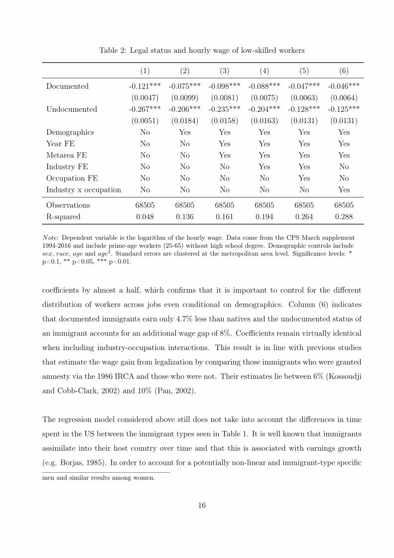
Table 2: Legal status and hourly wage of low-skilled workers

(1) (2) (3) (4) (5) (6)

Documented -0.121*** -0.075*** -0.098*** -0.088*** -0.047*** -0.046***(0.0047) (0.0099) (0.0081) (0.0075) (0.0063) (0.0064)

Undocumented -0.267*** -0.206*** -0.235*** -0.204*** -0.128*** -0.125***(0.0051) (0.0184) (0.0158) (0.0163) (0.0131) (0.0131)

Demographics No Yes Yes Yes Yes YesYear FE No No Yes Yes Yes YesMetarea FE No No Yes Yes Yes YesIndustry FE No No No Yes Yes NoOccupation FE No No No No Yes NoIndustry x occupation No No No No No Yes

Observations 68505 68505 68505 68505 68505 68505R-squared 0.048 0.136 0.161 0.194 0.264 0.288

Note: Dependent variable is the logarithm of the hourly wage. Data come from the CPS March supplement1994-2016 and include prime-age workers (25-65) without high school degree. Demographic controls includesex, race, age and age2. Standard errors are clustered at the metropolitan area level. Significance levels: *p<0.1, ** p<0.05, *** p<0.01.

coefficients by almost a half, which confirms that it is important to control for the different

distribution of workers across jobs even conditional on demographics. Column (6) indicates

that documented immigrants earn only 4.7% less than natives and the undocumented status of

an immigrant accounts for an additional wage gap of 8%. Coefficients remain virtually identical

when including industry-occupation interactions. This result is in line with previous studies

that estimate the wage gain from legalization by comparing those immigrants who were granted

amnesty via the 1986 IRCA and those who were not. Their estimates lie between 6% (Kossoudji

and Cobb-Clark, 2002) and 10% (Pan, 2002).

The regression model considered above still does not take into account the differences in time

spent in the US between the immigrant types seen in Table 1. It is well known that immigrants

assimilate into their host country over time and that this is associated with earnings growth

(e.g. Borjas, 1985). In order to account for a potentially non-linear and immigrant-type specific

men and similar results among women.

16

Figure 5: Wage gap to natives

−.2

5−

.2−

.15

−.1

−.0

50

Wage g

ap to n

atives

0−5 6−10 11−15 16−20 21−25 >25Years in US

Documented Undocumented

Note: The wage gaps result from a regression with the full set of controls as in column (6) of Table 2including workers with at most a high school degree. Vertical dashed lines show 10% confidence intervals.

growth in hourly wages over time, I augment the wage regression by an interaction between

the documented and undocumented immigrant dummies and years in US, which I group in six

5-year intervals (1-5, 6-10, 11-15, 16-20, 20-25 and >25) denoted by y = 1, ...6. The equation

for immigrants therefore takes the following form:

lnwiyt = β0 + β1yDit + β2yUit + φt +X ′itγ + εit.

Figure 5 plots the wage gap to natives for both immigrant types for each interval of years

in the US. To increase the number of immigrants observations per interval, I also include

high school graduates in the regression underlying the figure and add a dummy indicating

having completed high school as educational control.12 The wage gaps of documented and

undocumented immigrants residing in the US for at most 5 years are around 15% and 20%

respectively. The speed of assimilation is almost identical for both types of immigrants during

the first 20 years, however, after that the assimilation of undocumented immigrants slows down.

Earning only 2% less than natives, documented workers have almost fully assimilated after 2512Coefficients are almost identical but somewhat less precisely estimated when including high school dropouts

only.

17

Figure 6: Unemployment rates of low-skilled workers

0

.05

.1

.15

.2

Unem

plo

ym

ent ra

te

1995m1 2000m1 2005m1 2010m1 2015m1Date


Note: The series are constructed from CPS basic monthly files.

years, at which point undocumented workers still earn around 12% less. Thus, there are two

important take-aways from Figure 5. First, even accounting for the length of stay in the US,

there is still a large wage gap between documented and undocumented immigrants. Second,

the gap to natives is initially large and disappears through assimilation for the former but not

for the latter.

3.2 Unemployment and Transition Rates

I now turn to the analysis of the difference in unemployment and transition rates between em-

ployment and unemployment. The data used in this subsection are the CPS basic monthly files,

in which some of the variables for the identification of legal respondents, e.g. social security

benefits or health insurance, are not available. However, I show in the Appendix that in the

monthly data still at least 90% of low-skilled illegal immigrants are correctly identified (see

Appendix, Figure 18).

Figure 6 plots the unemployment rates of low-skilled workers. Both types of immigrants have

virtually the same rate of unemployment, which is significantly lower than the one of natives,

(except in the very beginning of the sample period). Contrary to the findings for wages, this

18

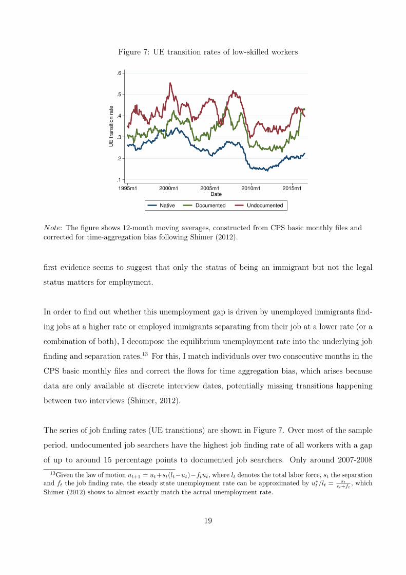
Figure 7: UE transition rates of low-skilled workers

.1

.2

.3

.4

.5

.6

UE

tra

nsitio

n r

ate

1995m1 2000m1 2005m1 2010m1 2015m1

Date


Note: The figure shows 12-month moving averages, constructed from CPS basic monthly files andcorrected for time-aggregation bias following Shimer (2012).

first evidence seems to suggest that only the status of being an immigrant but not the legal

status matters for employment.

In order to find out whether this unemployment gap is driven by unemployed immigrants find-

ing jobs at a higher rate or employed immigrants separating from their job at a lower rate (or a

combination of both), I decompose the equilibrium unemployment rate into the underlying job

finding and separation rates.13 For this, I match individuals over two consecutive months in the

CPS basic monthly files and correct the flows for time aggregation bias, which arises because

data are only available at discrete interview dates, potentially missing transitions happening

between two interviews (Shimer, 2012).

The series of job finding rates (UE transitions) are shown in Figure 7. Over most of the sample

period, undocumented job searchers have the highest job finding rate of all workers with a gap

of up to around 15 percentage points to documented job searchers. Only around 2007-200813Given the law of motion ut+1 = ut+st(lt−ut)−ftut, where lt denotes the total labor force, st the separation

and ft the job finding rate, the steady state unemployment rate can be approximated by u∗t /lt = stst+ft

, whichShimer (2012) shows to almost exactly match the actual unemployment rate.

19

Figure 8: EU transition rates of low-skilled workers

.02

.03

.04

.05

.06

EU

tra

nsitio

n r

ate

1995m1 2000m1 2005m1 2010m1 2015m1

Date


Note: The figure shows 12-month moving averages, constructed from CPS basic monthly files andcorrected for time-aggregation bias following Shimer (2012).

and at the end of the period, the latter have a similar rate. From 2000 on, natives perma-

nently have the lowest job finding rate with the difference to undocumented immigrants being

up to 25 percentage points. Given the similar level of the unemployment rate of documented

and undocumented workers seen in Figure 6, we expect a higher separation for undocumented

counteracting the higher job finding rate. This is confirmed by Figure 8: the EU transition

rate series of documented immigrants is close to the series of natives, while it over most of the

period higher for undocumented.

Altogether, the decomposition in transition rates suggest that, although the unemployment

rates of documented and undocumented workers almost exactly coincide, the latter are char-

acterized by much more frequent transitions in and out of employment. Moreover, the figures

show that the unemployment gap between natives and immigrants is primarily driven by a

differential in job finding rates. This is a surprising finding in the light of results of previous

studies suggesting that the variation of unemployment rates across workers (e.g. skill types in

Mincer, 1991) is almost solely driven by differing separation rates. Job finding on the other

hand has been found to mainly account for cyclical fluctuations of unemployment over time

20

Table 3: Legal status and UE transition of low-skilled workers

(1) (2) (3) (4) (5) (6)

Documented 0.074*** 0.065*** 0.075*** 0.073*** 0.071*** 0.072***(0.0047) (0.0067) (0.0082) (0.0076) (0.0077) (0.0076)

Undocumented 0.138*** 0.122*** 0.139*** 0.136*** 0.136*** 0.137***(0.0054) (0.0075) (0.0097) (0.0100) (0.0107) (0.0109)

Demographics No Yes Yes Yes Yes YesYear FE No No Yes Yes Yes YesState FE No No Yes Yes Yes YesIndustry FE No No No Yes Yes NoOccupation FE No No No No Yes NoIndustry x occupation No No No No No Yes


Note: Dependent variable is the probability of a UE transition. Data come from the CPS basic monthly files1994-2014 and include prime-age workers (25-65) without high school degree matched over two consecutivemonths. Demographic controls include sex, race, age and age2. Standard errors are clustered at the statelevel. Significance levels: * p<0.1, ** p<0.05, *** p<0.01.

(Shimer, 2012).

The transition rate differences might be explained by the demographic or occupational het-

erogeneity between the worker types but not the type itself. I therefore estimate a linear

probability model including demographic, industry and occupational controls analogous to the

wage regressions in the previous subsection. The dependent variable is a dummy indicating

a transition from unemployment to employment or, respectively, employment to unemployment.

The regression results for job finding rates (UE transitions) are reported in Table 3. It con-

firms the pattern seen in Figure 7: both types of immigrants find jobs faster than natives and

undocumented workers even faster than documented ones. Controlling for observables does

not influence the results, which are almost identical across all specifications. With the aver-

age monthly job finding probability of all workers being around 23%, the coefficients suggest

that documented workers find jobs with a probability that is around one third higher than the

21

Figure 9: Job finding rate gap to natives

0.0

5.1

.15

.2JF

R g

ap to n

atives

0−5 6−10 11−15 16−20 21−25 >25Years in US


Note: The gaps result from a regression with the full set of controls as in column (6) of Table 2 includingworkers with at most a high school degree. Vertical dashed lines show 10% confidence intervals.

average and undocumented workers with a probability that is even 60% higher than the average.

Analogously to Figure 5, Figure 9 plots the predicted difference in job finding rates of immi-

grants to natives depending on time in the US as a result from regression specification (6)

with an interaction between the immigrant dummies and 6 categories for years in the US. The

results are robust to taking into account the duration of stay in the US as there is a permanent

difference in job finding rates of 6 to 8 percentage points between the documented and undoc-

umented immigrants. As for wages, the gap narrows over time for both, although it does not

disappear completely after having spent more than 25 years in the US for the documented.

Table 4 shows the regression results with EU transitions as the dependent variable. In order to

be consistent with the sample of the wage regressions, I only consider separations from full-time

jobs. Further, I only consider transitions to unemployment, if the reason for unemployment

is either "job loser" or "job leaver".14 Including demographic variables but no further con-

trols, there is no significant difference in the separation rates between worker types. With the14The other unemployment reasons are: "temporary job ended", "re-entrant" and "new-entrant".

22

Table 4: Legal status and EU transition of low-skilled workers

(1) (2) (3) (4) (5) (6)

Documented -0.001* -0.001 -0.001*** -0.002*** -0.003*** -0.003***(0.0004) (0.0005) (0.0005) (0.0005) (0.0005) (0.0004)

Undocumented 0.001 -0.001 -0.002** -0.003*** -0.006*** -0.006***(0.0005) (0.0008) (0.0009) (0.0007) (0.0007) (0.0007)



Note: Dependent variable is the probability of an EU transition. Data come from the CPS basic monthly files1994-2014 and include prime-age workers (25-65) without high school degree matched over two consecutivemonths. Demographic controls include sex, race, age and age2. Significance levels: * p<0.1, ** p<0.05, ***p<0.01.

full set of controls, the coefficients suggest that documented immigrants have a 0.3 percent-

age points and undocumented immigrants a 0.6 percentage points lower separation probability

than natives. Quantitatively, these differences between worker types are smaller compared to

the differences in job finding rates. This also holds when relating the differences to the much

smaller average separation probability, which is around 1.6%.

Figure 10 plots the predicted difference in separation rates of immigrants depending on length

of stay in the US. Conditional on time in the US, there is no significant difference in separation

rates between immigrants. Both documented and undocumented workers have lower separation

rates initially and fully catch up to natives after more than 25 years in the country.

23

Figure 10: Separation rate gap to natives

−.0

06

−.0

04

−.0

02

0.0

02

.004

SR

gap to n

atives

0−5 6−10 11−15 16−20 21−25 >25Years in US


Note: The gaps result from a regression with the full set of controls as in column (6) of Table 2 includingworkers with at most a high school degree. Vertical dashed lines show 10% confidence intervals.

3.3 Reservation Wages

In the Mortensen-Pissarides search and matching model (Mortensen and Pissarides, 1994), the

utility of a worker does not only depend on wage earnings but also on the probability of finding

a job and the expected length of the job spell. Thus, besides wages, job finding and separation

rates are crucial determinants of the values of working and searching for a job. Formally, this

is summarized by the flow value for worker i of being unemployed, which in its basic form is

given by:15

rUi = zi + fiwi − zi

r + si + fi. (1)

The value depends positively on unemployment benefits zi (which also include the value of

leisure or home production and is net of job-search costs), job finding rate fi and wage wi

(which depends on the bargaining power of a worker), and negatively on the interest rate r

and the rate of job separation si. Being the opportunity costs to working, the flow value of15This follows from the flow value of working rWi = wi + si(Ui − Wi) combined with the flow value of

unemployment rUi = zi + fi(Wi − Ui)

24

being unemployed equals the reservation wage at which a worker is indifferent between staying

unemployed and having a job, i.e. wi = rUi = rW (wi). Expression (1) shows how changes in

the exogenous variables zi, r and si affect the endogenous variables fi and wi. A fall of the

reservation wage, e.g. because of a decrease in zi or an increase in si, lowers the threat point of

a worker and therefore decreases his negotiated wage. This induces job creation due to higher

firm profits, which increases job finding and therefore counteracts the reservation wage decline.

One explanation for the lower wages of undocumented compared to documented workers is

that the former are characterized by a lower zi. If low-skilled immigrants, and particularly

undocumented ones, are disadvantaged relative to natives in terms of job search conditions and

unemployment benefits, this lowers their reservation wage. However, as the reservation wage

also depends on transition rates, it is not clear that a difference in paid wages automatically

translates into a difference in reservation wages. As shown above, immigrants have higher job

finding and lower separation rates, which tends to increase their reservation wages relative to

natives. In order to provide some conclusive evidence on reservation wage differentials, I com-

pute reservation wages according to equation (1) for natives, documented and undocumented

immigrants in each sample year.

I obtain the series of wages and transition rates by first calculating the average for natives in

each year and then running a model corresponding to specification (6) of the regression ta-

bles, in which the coefficients of Dit and Uit are allowed to vary over time by being interacted

with the year dummies. I compute the hourly wages and monthly transition rates fi and si

of documented and undocumented immigrants for each year by applying the gap given by the

time-varying coefficients of the respective dummies to the corresponding series calculated for

natives. In order to convert hourly wage to monthly income wi , I assume 40 hours worked per

week. For simplicity, the unemployment flow payment is computed as zi = 0.4wi. The monthly

interest rate is set to 0.004 as in Shimer (2005).

Figure 11 displays the resulting series of reservation wages wN , wD and wU . Despite having

the highest job finding and lowest separation rate, undocumented immigrants have by far the

lowest reservation wage, which is around $600 below the reservation wage of natives throughout

25

Figure 11: Reservation Wages

1000

1200

1400

1600

1800

Reserv

ation W

age

1995 2000 2005 2010 2015Year


Note: The gaps underlying the calculation result from a regression with the full set of controls as in column(6) of Table 2.

the whole period. Documented immigrants on the other are only around $200 below natives.

This confirms that the negative effect of a lower wage overcompensates the positive effect of a

higher job finding and lower separation rate on the reservation wage of immigrants.

While lower reservation wages can account for the observed wage differences between worker

types in a standard search and matching model with random matching, it cannot account for

the observed large differences in job finding rates, which are always equal across worker types.

I therefore propose a model that incorporates non-random hiring in the search and matching

framework in the next section. This model provides an intuitive explanation for why undocu-

mented immigrants find jobs faster: when having the choice, firms prefer to hire undocumented

workers because they can pay them lower wages.

26

4 Model

This section presents a labor market model extending the canonical search and matching frame-

work (Mortensen and Pissarides, 1994) with non-random hiring, whose implementation is based

on the hiring mechanism in Barnichon and Zylberberg (2014). They depart from the assumption

that matching is strictly random and instead allow firms to gather and rank several applications

and hire the worker they receive the highest surplus from. This mechanism is not only intuitive,

but also consistent with evidence concluding that firms usually interview many applicants at

once (Barron et al., 1985, Barron and Bishop, 1985). For the sake of simplicity, I only distin-

guish two worker types: documented workers (including natives and documented immigrants)

and undocumented immigrants.

4.1 Basics, Matching Mechanism and Wage Bargaining

There is a continuum of measure one of risk-neutral, infinitely lived workers in the economy,

who can be either documented or undocumented. Their type is denoted by i ∈ {D,U} and each

represents an exogenous share ωi of the total work force P . A worker of a given type is either

employed and inelastically supplies one unit of labor earning wage wi, or unemployed, receiving

a flow payment zi. I assume that the flow payment consists of unemployment benefits zUI and

home production zH . While home production is the same for both types, undocumented work-

ers are not eligible for unemployment benefits and therefore we have zD = zUI +zH > zU = zH .

I also allow the bargaining powers βD and βU to differ between worker types, accounting for the

fact that undocumented immigrants are likely to have a lower bargaining power in negotiating

wages because hiring an unauthorized worker is unlawful. Moreover, I introduce the possibility

for an unauthorized worker to be detected and removed. I allow the probability of detection

to be potentially different for an employed and an unemployed worker.16 I denote the rate of

removal for an employed worker by λW and for an unemployed worker by λU . Removal not

only implies job loss (in case of being employed), but also the loss of an utility amount R > 0,16This is motivated by the fact that under the presidency of George W. Bush, conducting worksite raids and

arresting undocumented workers (with subsequent deportation in many cases) was the prevalent method to takeaction against illegal hiring. Under the presidency of Barack Obama, this policy changed towards targetingemployers, which usually led to undocumented workers being fired, but in fewer cases being deported (see forexample http://www.nytimes.com/2010/07/10/us/10enforce.html?_r=0).

27

http://www.nytimes.com/2010/07/10/us/10enforce.html?_r=0

which captures the disutility associated with being removed.

There is a large measure of risk-neutral firms, which enter the economy by posting vacancies

at a cost c > 0. A firm paired with a worker produces output y, which is independent of the

worker type. I assume that workers can apply at most to one job and that their application is

randomly allocated to a vacancy by an urn-ball matching function (Butters, 1977). Hence, due

to coordination frictions, some firms will receive multiple applications while others will receive

none. With a large number of vacancies V and a large number of homogeneous applicants, the

probability for a firm to be matched with exactly k applicants can be approximated by a Poisson

distribution: P (k) = qk

k!e−q with q being the candidate to vacancy ratio. To fit the model to the

data, I introduce a matching efficiency parameter µ, thereby proceeding as Blanchard (1994).

This implies that every period, a worker sends out an application with probability µ. Thus,

the probability to be matched with kD documented and kU undocumented workers is given by:

P (kD, kU) =(µqD)kD

kD!e−µqD

(µqU)kU

kU !e−µqU (2)

where qi = ui/V , i.e. the ratio of candidates of type i to vacancies or "queue length".

I adopt the wage bargaining mechanism between firm and worker as described in Barnichon

and Zylberberg (2014). Job finding rate and bargaining position of an applicant will depend

on the labor market tightness, i.e. the total number of candidates to vacancies, as well as the

composition of the candidate pool. An increase in the share of workers in the pool that firms

hire preferably will always decrease job finding of the workers already present, although it will

increase average job finding of the total workforce (as it raises the share of the type with higher

job finding). Whenever a firm receives one or more applications, the firm makes a take-it-or-

leave-it offer to its highest ranked candidate with probability (1−βi), capturing all the surplus

by offering a wage making the candidate indifferent to her outside option. With a probability

βi, the applicants send offers to the firm with the outcome that the best candidate demands a

wage making the firm indifferent between her and the second-best candidate. Hence, if a firm is

only matched with one applicant, the expected payoffs are as in the standard Nash bargaining

game and in expectation the worker receives a share βi of the surplus Si. As undocumented

28

have lower reservation wages than documented workers (for an expression of the reservation

wages see below), we have that SU > SD. If a firm faces more than one applicant, there are

three different cases to distinguish when determining the match surplus for the worker SW :

a) All applicants are of the same type: Candidates will bid their wages down to their reser-

vation wage and the firm captures all the surplus: SW = 0.

b) The firm has more than one undocumented applicant. As in case a), the applicant will

only receive her reservation wage: SW = 0.

c) The firm has one undocumented and at least one documented applicant. The undocu-

mented worker will send an offer to make the firm indifferent between hiring him and a

documented worker with probability βi and therefore in expectation capture a share βU

of the surplus generated over and above the surplus generated by a documented worker:

SW = βU(SU − SD)

Hence, a worker can only extract any surplus from a match when being the only candidate that

is strictly better than the other candidates applying to the same firm.

4.2 Workers

In a continuous time setting, the flow values of being employed for legal and illegal workers are

given by:

rWD = wD + s(UD −WD(w)) (3)

rWU = wU + s(UU −WU(w)) + λW (UU −R−WU(w)). (4)

As implied by equation (5), I assume that undocumented workers still receive their unemploy-

ment value after deportation, which is not essential for the results but improves the tractability

29

Table 5: Wage distribution

Case Probability WageDocumented Undocumented

1) No competitors f1 = e−µqDe−µqU wD + βD(y − wD) wU + βU(y − wU)

2) Only D competitors f2 = (1− e−µqD)e−µqU wD wU + βU((1 + λW

r+s)wD − λW

r+sy − wU)

3) At least one U competitor f3 = 1− e−µqU rUD = wD wU

of the model.17 The flow values of being unemployed rUi are given by

rUD = zD +

∫max(WD(w)− UD, 0)dFD(w) (5)

rUU = zU +

∫max(WU(w)− UU , 0)dFU(w)− λUR (6)

with F denoting the distribution of the negotiated wages, which depends on the number of

candidates applying for the same job.

To find the reservation wage wi, note that when earning the reservation wage a worker is

indifferent between working and staying unemployed, so that we get rUD = rW (wD) = wD and

rUU = rW (wU) = wU − λWD. Hence, using this with (4) and (5), we get for legal workers:

wD = zD +1

r + s

∫ ∞wD

(w − wD)dFD(w). (7)

For undocumented workers we get:

wU = zU +1

r + s+ λW

∫ ∞wU

(w − wU)dFU(w) + (λW − λU)︸︷︷︸∆λ

R. (8)

The wage distribution F , which can be derived from the above described matching probabilities

and wage bargaining mechanism, is summarized in Table 5.18

17This can be rationalized by defining R = R+ UU − UH , where UH is the (exogenous) unemployment valuea removed worker receives in his home country after deportation and R is the disutility directly received frombeing removed (e.g. temporary arrest, moving costs, family separation etc.). Being an endogenous variable, UU

cancels out in the term in the last bracket in equation (5). However, as this would complicate calculations, Iinstead assume R = R+ UU − UH , where UU and therefore R are exogenous.

18The undocumented wage in case 2) is derived from (y−wU )/(r+ s+λW ) = (y−wD)/(r+ s), i.e. equatingthe firm surplus when hiring an undocumented with the firm surplus when hiring a documented worker.

30

Combining the distribution of wages with equations (7) and (8), we get the reservation wages

as

wD =zD + βD

r+sf1y

1 + βDr+s

f1

(9)

wU =zU + βU

r+s+λW(f1y + f2( λ

W

r+sy + (1 + λW

r+s)wD) + ∆λR

1 + βUr+s+λW

e−µqU(10)

If all workers were identical, i.e. zD = zU , βD = βU and λW=λU=0, the reservation wages of

both types would be equal. A decrease in either zi or βi leads to a decline in the reservation

wage for worker type i in equilibrium. As I assume zD > zU , a sufficient condition for wD > wU

is βD ≥ βU . This condition is also sufficient if R = 0 or R is very small, as then λW just acts

as a separation rate differential between documented and undocumented workers and a rise in

this differential decreases wU relative to wD. If ∆λR is large enough, i.e. the removal rate is

much higher for the employed than for the unemployed, we could have wD < wU . However,

as this is not consistent with the data, all model parameter constellations used throughout the

paper will ensure that wD > wU is satisfied. Given this inequality holds, the wage distribution

implies that the expected wage of a undocumented workers is smaller than the expected wage

of a documented worker and that firms always prefer to hire the former.

The job finding rates for each worker type can be derived from fi = mi/ui, where mi denotes

the number of vacancies filled by worker type i. The probability of a vacancy being filled by a

documented is given by f2, while the probability of a vacancy being filled by an undocumented

worker is given by f3. Thus, the job finding rates are:

fD = f2V/uD =(1− e−µqD)e−µqU

qD(11)

fU = f3V/uU =1− e−µqU

qU> fD (12)

31

4.3 Firms

On the firm side, the flow values of hired documented and undocumented workers are given by

rJD(π) = π + s(V − JD(w)) (13)

rJU(π) = π + (s+ λW )(V − JU(w)) (14)

and the flow value of posting a vacancy rV is given by

rV = −c+

∫max(Ji(π)− V, 0)dG(π, i). (15)

The number of posted vacancies is determined by the free entry condition V = 0, setting

vacancy costs equal to expected match surplus for the firm:

c =

∫ ∞0

Ji(π)dG(π, i) (16)

The distribution of profits shown in Table 6 can again be derived for every case considering the

wages paid and the respective probabilities.

Table 6: Profit distribution

Case Probability Profit Hire1) One D, no U µqDe

−µqDe−µqU (1− βD)(y − wD) D2) One U, no D µqUe

−µqDe−µqU (1− βU)(y − wU) U3) > one D, no U (1− e−µqD − µqDe−µqD)e−µqU y − wD D4) > one U (1− e−µqU − µqUe−µqU ) y − wU U5) ≥ one D, one U µqUe

−µqU (1− e−µqD) y − wU − βU((1 + λW

r+s)wD − λW

r+sy − wU) U

4.4 Static Equilibrium

As in the standard search framework, the ratio of job seekers to vacancies for each worker

type is independent of the size of the total unemployment pool uD + uU . What determines

the equilibrium is the ratio of documented to undocumented workers among the unemployed

uU/uD = qU/qD. With the given distribution of profits, it can easily be verified that the higher

32

is this ratio, the higher is the probability of having at least one undocumented applicant and

therefore the higher are expected firm profits. Hence, while an increase in the unemployment

pool that leaves uU/uD unchanged does not affect the equilibrium as vacancies will increase

proportionally, a relative increase in uU compared to uD will lead to an increase in vacancies

that is overproportional to the increase of the total unemployment pool and vice versa.

In order to close the model, we need to consider the laws of motion of the number of unemployed

workers and the work force given by:

uD = s(ωDP− uD)− fDuD, (17)

uU = s(ωUP− uU) + uNU − fUuU − λUuU , (18)

P = uNU − λW (ωUP− uU)− λUuU , (19)

where uNU is the inflow of new undocumented immigrants, who I assume to be unemployed

initially. In order to keep the population constant and obtain a static equilibrium, I set uNU =

λW (ωU

P− uU) + λUuU . Thus, ouflows of deported immigrants are compensated by an equal

amount of inflows. With the normalization P = 1, the steady state of the number of unemployed

workers of each type is therefore given by:

u∗D =ωDs

s+ fD(20)

u∗U =ωU(s+ λW )

s+ λW + fU(21)

The static solution of the model is determined by equations (9), (10), (11), (12), (13), (14),

(16), (20), (21), and consists of the equilibrium candidate-vacancy ratios q∗D and q∗U .

5 Calibration

In the following, I describe the calibration of the model, for which I use several methods. Some

parameters are set equal to their data equivalents or are taken from the literature, others are

chosen to jointly match some moments of the data. An overview of the calibrated parameter

values can be found in Table 15 in the Appendix.

33

The level of productivity y and the documented population ωD are both normalized to 1. The

monthly discount factor δ is set equal to 0.9966, implying an annual interest rate of 4%. Instead

of choosing the population shares ωD and ωU and determining the ratio uU/uD from the steady

state equation for unemployment, I fix uU/uD at 0.27, which is the mean of this ratio over the

period 1994-2014. I do so, because my target for the job finding rate gap is the coefficient of

the illegal dummy in the regression of Table 3 and this gap will determine the equilibrium ratio

uU/uD resulting from the model, given that ωD and ωU are fixed. The empirical ratio uU/uD

on the other hand is generated by the unconditional transition rates in the data and therefore

inevitably different to the model result, if the population ratio ωU/ωD is set to its data equiva-

lent. After fixing uU/uD, the population ratio implied by the steady state of unemployment in

the model can be computed by solving (15) for ωi.19

Estimates of the flow payment of unemployment range between 0.4 (the upper end of the

range of income replacement rates in Shimer (2005)) and 0.955 in Hagedorn and Manovskii

(2008). I choose an intermediate value of 0.71 for zL as used in Hall and Milgrom (2008) and

Pissarides (2009). Computing the unemployment benefits as zUI = 0.4wL, where wL is the

average wage of legal workers, which is around 0.97, gives zUI = 0.39. Hence, zD − zUI yields

zH = zU = 0.32. After correction for time aggregation bias, I get an average separation rate

for low-skilled native workers of 0.031. As Table 4 suggests that documented immigrants have

a separation rate that is 0.003 lower than the rate of natives and the immigrant share among

documented workers is around 0.4, I set sD = 0.6 · 0.031 + 0.4 · 0.028 ≈ 0.030. The difference

between the separation rates of undocumented immigrants and natives is 0.006 and thus I set

sU = 0.031− 0.006 = 0.025.

In order to obtain a value of the removal rate, I use yearly figures of unauthorized immigrants

that are deported through so called "interior removals" from the Department of Homeland

Security, which are available from 2008 through 2015.20 I convert these figures to a monthly

frequency, divide them by the total number of undocumented immigrants residing in the US19The model implies ωU/ωD = 0.31, which is very close to the ratio of 0.30 in the data20"Interior removals" refer to deportations of immigrants that are not apprehended directly at the border.

The figures are available at https://www.ice.gov/removal-statistics

34

in the respective year and take the average across years. The resulting rate is 0.0013. Unfor-

tunately, to the best of my knowledge there is no information on the employment status of

deported immigrants available. I therefore assume λW = λU = 0.0013 in the baseline calibra-

tion and show how the predictions change when deviating from this assumption, i.e. ∆λ 6= 0.

The value of the disutility of deportation R only matters if ∆λ 6= 0 and in this case I set

R = 100. I will check robustness of the results to different choices of R.

This leaves four remaining parameters to be determined, c, βD, βU and the matching efficiency

µ with three moments from the data to be matched. These are the ratio of the average wages

paid to workers wU/wD and the job finding rates fD and fU . In order to get rid of one pa-

rameter, I proceed as many papers in the search literature and assume an average bargaining

power in the economy of 0.5. Hence, I restrict βD and βU to satisfy ωD

ωD+ωUβD + ωU

ωD+ωUβU = 0.5.

This leaves the difference between βD and βU along with c and µ to be matched. According

to the sixth column of Table 2, documented immigrants earn 4.6% less than natives. Taking

natives as a reference group with a normalized wage of 1, I can then compute the wage level

of all documented workers using the population proportions as 0.6 · 1 + 0.4 · 0.954 ≈ 0.982.

With undocumented workers earning 12.5% less than natives, the wage ratio is then given by

wU/wD = 0.875/0.982 ≈ 0.89. In order to get the job finding rates, I proceed similarly as for

the separation rates. The time aggregation bias corrected job finding rate of low-skilled natives

is around 0.24. Considering the coefficients in the sixth column of Table 3, the job finding rates

are fD = 0.6 ·0.241+0.4 ·0.312 ≈ 0.27 and fU = 0.241+0.137 ≈ 0.38. The resulting parameters

are βL = 0.67, βI = 0.15, µ = 0.41 and c = 0.72.

6 The Effect of Undocumented Immigration

6.1 Job Creation and Competition Effect

The model outlined in the previous section features two effects of a rise in the population share

of undocumented workers that have opposing impacts on the job finding rate of documented

workers. With a higher probability of receiving an application from an undocumented, expected

35

wage costs of firms go down and therefore more vacancies are posted. This job creation effect

increases documented workers’ job finding and is also present in the standard framework with

random hiring. The competition effect on the other hand decreases job finding rates of both

worker types as the probability of competing with an undocumented for a job and thus not

being hired rises. The two effects can be shown by recalling the expression for the job finding

rate of documented workers (11). An increase in vacancies decreases the queue length qD. By

taking the partial derivative with respect to qD we see that the marginal effect of an increase

in qD on fD is negative:

∂fD∂qD

=e−µqD(1 + µqD)− 1

q2D

e−µqU < 0 ∀ qD > 0.

Hence, the job creation effect is always positive. The competition effect can be demonstrated

by taking the partial derivative with respect to qU , which increases as a result of a rise in the

undocumented population share:

∂fD∂qU

= −µ(1− e−µqD)

qDe−µqU < 0 ∀ qU > 0,

∂fU∂qU

=e−µqU (1 + µqU)− 1

q2U

< 0 ∀ qU > 0.

Thus, the total effect of an increase in ωU is ambiguous for documented and negative for

undocumented workers:

dfDdωU

=∂fD∂qD︸︷︷︸<0

dqDdωU︸︷︷︸<0︸︷︷︸

job creation effect

+∂fD∂qU︸︷︷︸<0

dqUdωU︸︷︷︸>0︸︷︷︸

competition effect

≶ 0, (22)

(23)dfUdωU

=∂fU∂qU︸︷︷︸<0

dqUdωU︸︷︷︸>0︸︷︷︸

competition + job creation effect

< 0. (24)

The larger is the difference between worker types, the larger is the difference in their reservation

wages and therefore the higher is the increase in expected firm profits and the number of

36

vacancies posted following an increase in ωU . Hence, the job creation effect tends to zero when

the worker types become identical and gets larger when increasing the difference between them,

eventually letting dfD/dωU become positive.

6.2 Simulating Undocumented Immigration

In order to find out which of the two effects dominates with the calibration that replicates

the data, I solve for the steady state equilibrium varying the undocumented population share

ωU/(ωD + ωU). Figure 12 plots the resulting steady state queue lengths, job finding rates,

average wages and reservation wages by worker type and in the aggregate. The upper left panel

shows a sharp decline in the queue length of documented workers, indicating a large increase in

vacancies and hence a strong job creation effect. Accordingly, their job finding rate increases

with the arrival of more undocumented workers, which confirms that the job creation effect is

strong enough to dominate the competition effect. Average wages of both worker types increase

as a result of a reservation wage increase induced by the additional vacancies posted. However,

as the share of workers earning a lower wage goes up, the aggregate average wage paid drops.

The reservation wage is equal to the value of unemployment for undocumented workers and

therefore functions as a measure of welfare. The lower right panel suggests that the welfare of

documented workers increases through undocumented immigration. For undocumented immi-

grants we have wU = rUU +λWR. As λWR is held fixed for now, the increase in undocumented

workers’ reservation wages also implies a rise in welfare for them.

Figure 13 shows the hypothetical effect of undocumented immigration under the assumption

that there exists no bargaining power difference between the worker types. In this case, the

wage gap only comes from the difference in unemployment benefits and the removal risk (the

benchmark is plotted in dashed lines for comparison). The purpose of this figure is twofold.

First, it illustrates that most of the reservation wage gap is generated by the bargaining power

difference as under the assumption of equal bargaining powers there is only a gap of around 2%

between the reservation wages of documented and undocumented workers. Second, it shows

that with such a small reservation wage gap, the competition effect is the dominating one.

Although there are still additional vacancies created as indicated by the decreasing aggregate

37

Figure 12: Equilibrium depending on undocumented share

0.1 0.15 0.2 0.25 0.3 0.35 0.4 0.45 0.5 0.55 0.6

Share of undocumented workers

0

0.5

1

1.5

2

2.5

3Queue length

Documented Undocumented Aggregate

0.1 0.15 0.2 0.25 0.3 0.35 0.4 0.45 0.5 0.55 0.6


22

24

26

28

30

32

34

36

38

40Job finding

0.1 0.15 0.2 0.25 0.3 0.35 0.4 0.45 0.5 0.55 0.6


0.86

0.88

0.9

0.92

0.94

0.96

0.98

1Average wage

0.1 0.15 0.2 0.25 0.3 0.35 0.4 0.45 0.5 0.55 0.6


0.85

0.9

0.95

1Reservation wage

queue length, the job finding rate curve of documented workers is now falling as job creation is

not strong enough to counteract the increased job competition through undocumented workers.

This exercise confirms that the findings are sensitive to the parameters and therefore I next

check whether the predictions of Figure 12 are robust to allowing ∆λ 6= 0 and to the choice of

R. In particular, I consider the extreme case in which only employed undocumented workers

can be detected and deported, i.e. λU = 0 and λW = ∆λ. I recalibrate λW following the same

method of calibration as described in section 5 but dividing monthly interior removals by the

total number of employed undocumented immigrants instead of all undocumented immigrants.

The resulting probability is 0.0022. Since ∆λ is strictly greater than zero, R always has a

positive effect on wU . Thus, it affects undocumented immigrants’ wages and as a consequence

the wage gap between worker types. The value of R also affects job finding rates because a rise

in wU makes hiring undocumented workers more expensive, which mutes the vacancy creation

effect. Therefore, it is necessary to reestimate c, βL and βI in order to match the moments

from the data after a change in R. Figures 19, 20 and 21 in the Appendix show the effect of

undocumented immigration for the calibrations R = 0, R = 100 and R = 200 and compare it

38

Figure 13: Equilibrium depending on undocumented share with βD = βU = 0.5

0.1 0.15 0.2 0.25 0.3 0.35 0.4 0.45 0.5 0.55 0.6


0

0.5

1

1.5

2

2.5

3Queue length


0.1 0.15 0.2 0.25 0.3 0.35 0.4 0.45 0.5 0.55 0.6


0.2

0.22

0.24

0.26

0.28

0.3

0.32

0.34

0.36

0.38

0.4Job finding

0.1 0.15 0.2 0.25 0.3 0.35 0.4 0.45 0.5 0.55 0.6


0.86

0.88

0.9

0.92

0.94

0.96

0.98

1Average wage

0.1 0.15 0.2 0.25 0.3 0.35 0.4 0.45 0.5 0.55 0.6


0.85

0.9

0.95

1Reservation wage

Note: Benchmark from Figure 12 in dashed lines

to the benchmark calibration with ∆λ = 0 (dashed lines). Queue lengths, job finding rates and

average wages are virtually unaffected by the choice of R after c, βD and βU are recalibrated.

Only the reservation wage of undocumented workers changes, moving in the same direction as R.

In sum, undocumented immigration is unambiguously beneficial for documented workers. This

is because the immigration of cheaper workers stimulates vacancy creation and this more than

offsets the negative effect of increased competition on job finding for documented workers.

Despite their fall in job finding, also undocumented workers’ welfare increases through rising

wages.

7 The Effect of Removal Risk

In what follows, I investigate how the equilibrium depends on the deportation risk parameters

λW and λU and how their effect on the equilibrium changes with R.

39

Figure 14: Equilibrium depending on λW with λW = λU

0 0.1 0.2 0.3 0.4 0.5 0.6 0.7 0.8 0.9 1

λW

0.2

0.4

0.6

0.8

1

1.2

1.4

1.6

1.8

2Queue length


0 0.1 0.2 0.3 0.4 0.5 0.6 0.7 0.8 0.9 1

λW

26

28

30

32

34

36

38

40Job finding

0 0.1 0.2 0.3 0.4 0.5 0.6 0.7 0.8 0.9 1

λW

0.85

0.9

0.95

1Average wage

0 0.1 0.2 0.3 0.4 0.5 0.6 0.7 0.8 0.9 1

λW

0.82

0.84

0.86

0.88

0.9

0.92

0.94

0.96

0.98Reservation wage

Recalling equation (10), we know that the effect of λW on undocumented workers’ reservation

wage is ambiguous. Given R is zero or sufficiently small, λW tends to decrease wU acting like

a rise in the job separation probability. However, if the disutility associated with deportation

is high enough, a rise in λW increases wU because ∆λ, i.e. the risk of detection when employed

relative to the risk when unemployed, rises and therefore the compensation needed to accept

the risk of having a job goes up more strongly. Independently of the size of R, a higher λW

will mute the job creation effect because the surplus firms expect to make by hiring an undoc-

umented worker shrinks due to the larger separation risk. If R>0, the job creation effect is

additionally muted due to a higher risk compensation. This negative effect of λW on vacancy

creation is increasing in R. A rise in λU , the risk of being deported when unemployed, un-

ambiguously decreases the reservation wage because the opportunity cost to having a job falls

and hence undocumented workers accept lower wages. As the aim is simulating an exogenous

policy change by varying λW and λU , I use comparative statics and therefore do not recalibrate

the remaining parameters.

Figures 14 shows the effect of an increase in both λW and λU on the equilibrium keeping the

40

Figure 15: Equilibrium depending on λW with λU = 0.0013

0 0.05 0.1 0.15 0.2 0.25

λW

0

0.5

1

1.5

2

2.5Queue length


0 0.05 0.1 0.15 0.2 0.25

λW

22

24

26

28

30

32

34

36

38

40Job finding

0 0.05 0.1 0.15 0.2 0.25

λW

0.82

0.84

0.86

0.88

0.9

0.92

0.94

0.96

0.98

1Average wage

0 0.05 0.1 0.15 0.2 0.25

λW

0.8

0.82

0.84

0.86

0.88

0.9

0.92

0.94

0.96

0.98Reservation wage

population share of undocumented immigrants fixed.21 As ∆λ remains zero, the rise in the

removal rate only affects undocumented workers’ separation probability and hence the queue

length rises slightly as the surplus from hiring undocumented workers falls and firms create less

vacancies. This is reflected in a moderate fall in job finding rates of both worker types. While

wages of documented workers remain almost flat, wages of undocumented workers fall sharply

due to the direct effect of the lower match surplus on the reservation wage.

Figure 15 plots the equilibria for the case where only the removal risk when employed λW

rises e.g. through more frequent worksite raids. Now, the negative impact on queue length

and job finding is strongly enhanced because the surplus of hiring undocumented workers ad-

ditionally falls due to the increase in the wage compensation for the higher deportation risk

when employed, implying even less new vacancies posted. This is reflected by the strong rise

in documented immigrants’ reservation wages, which however do not reflect a higher welfare as

the rise in wU is counteracted by the rise in λWR.21This is equivalent to a calibration in which R = 0 and only λW increases as in both cases, a risk compensation

for accepting a job does not play any role.

41

In sum, the analysis in this section suggests that increased deportation efforts by the authorities

lower the welfare not only of the undocumented, but also of documented workers. This is

even more so the case, if efforts concentrate on worksite raids making it more risky (but still

worthwhile) for an undocumented immigrant to accept a job. The detrimental effect of worksite

raids would be even larger, if the model also considered penalties for firms hiring workers illegally

as this would mute vacancy creation further.22

8 Testing the Model Predictions

In the previous section I have shown that, at least qualitatively, the prediction that job finding

rates of all workers fall when the removal risk increases does not depend on the assumption

that this risk is the same for employed and unemployed workers nor on the assumption that

there is a disutility from removal.23 However, the prediction on wages does depend on these

assumptions: if ∆λ = 0, a higher removal risk decreases undocumented immigrants’ wages,

whereas if only λW (and thus ∆λ) increases, their wages are predicted to rise. Finding a nega-

tive effect of an exogenous change in the removal risk on the job finding rate of both workers

types and on wages of documented workers would provide evidence that the job creation effect

of undocumented immigration exists. Given the model is correct, finding a positive effect of a

removal risk shock on the wages of undocumented immigrants would suggest that firms indeed

have to pay them a risk compensation.

A possible source of variation in the deportation risk is provided by a change in state-wide immi-

gration legislation. Good (2013) examines the impact of omnibus immigration laws (introduced

in eleven US states since 2006) on population and employment of different demographic groups.

These laws address several issues at a time including work authorization, document-carrying

policy, public program benefits, human trafficking, local immigration law enforcement or deter-22I abstract from these penalties as there is no evidence that they are in fact large enough to play a significant

role for firm decisions. Moreover, their addition to the model would bring no further insight beside enhancingthe effect of a variation in λW .

23Recall from equation (10) that the risk compensation only depends on ∆λ, which is why assuming ∆λ = 0is equivalent to assuming R = 0 (apart from the welfare of undocumented workers, which varies with R butdoes not influence the equilibrium).

42

Table 7: Legal status, omnibus laws and UE transition of low-skilled workers

(1) (2) (3) (4) (5) (6)

Documented 0.071*** 0.063*** 0.075*** 0.073*** 0.071*** 0.072***(0.0048) (0.0070) (0.0084) (0.0078) (0.0079) (0.0077)

Undocumented 0.135*** 0.120*** 0.138*** 0.135*** 0.136*** 0.137***(0.0055) (0.0077) (0.0098) (0.0101) (0.0109) (0.0111)

Omnibus law -0.035*** -0.029*** -0.027*** -0.025*** -0.025*** -0.021***(0.0075) (0.0072) (0.0073) (0.0070) (0.0062) (0.0068)

Documented x omnibus 0.047 0.034* 0.020 0.017 0.017* 0.005(0.0288) (0.0199) (0.0134) (0.0135) (0.0094) (0.0111)

Undocumented x omnibus 0.051* 0.043 0.015 0.013 0.013 0.006(0.0272) (0.0379) (0.0328) (0.0326) (0.0300) (0.0294)




mination of legal status when arrested.24 Although it is to the best of my knowledge not verified

whether these laws have an impact on the removal risk, Good (2013) states that they have a

nature of "in general creating an environment in which there is a constant threat of document

verification and subsequent deportation." (Good, 2013, p. 4). Raphael and Ronconi (2009) and

Good (2013) both provide evidence that the implementation of omnibus immigration laws is

not endogenous to levels or changes in discriminatory attitudes or immigrant population size.

I therefore conclude that they are appropriate to capture an exogenous increase in the removal

risk.

In order to measure the effect of omnibus immigration laws on job finding, I rerun the regres-

sion with the job finding rate as dependent variable including a dummy indicating immigration24A full list of date of enactment by state and issues addressed can be found in Appendix 1 of Good (2013).

43

Table 8: Legal status, omnibus laws and hourly wage of low-skilled workers

(1) (2) (3) (4) (5) (6)

Documented -0.123*** -0.077*** -0.100*** -0.090*** -0.049*** -0.048***(0.0047) (0.0100) (0.0080) (0.0075) (0.0063) (0.0064)

Undocumented -0.269*** -0.208*** -0.238*** -0.206*** -0.131*** -0.128***(0.0052) (0.0186) (0.0158) (0.0163) (0.0130) (0.0130)

Omnibus law -0.089*** -0.097*** -0.062*** -0.056*** -0.052*** -0.052***(0.0193) (0.0183) (0.0182) (0.0169) (0.0157) (0.0171)

Documented x omnibus 0.076** 0.090*** 0.097*** 0.092*** 0.084*** 0.081***(0.0309) (0.0228) (0.0212) (0.0208) (0.0184) (0.0198)

Undocumented x omnibus 0.085*** 0.095*** 0.107*** 0.100*** 0.093*** 0.092***(0.0300) (0.0322) (0.0300) (0.0282) (0.0259) (0.0290)

Demographics No Yes Yes Yes Yes YesYear FE No No Yes Yes Yes YesMetarea FE No No Yes Yes Yes YesIndustry FE No No No Yes Yes NoOccupation FE No No No No Yes NoIndustry x occupation No No No No No Yes



omnibus laws to be in force in the state of residence of a survey respondent during the inter-

view year. I interact this dummy additionally with the legal and illegal immigrant indicator in

order to allow the effect of omnibus immigration legislation to vary across immigrant status.

The results are shown in Table 7. The coefficients in the third row capture the effect of the

implementation of the laws on native workers. The preferred specification in the last column

indicates that omnibus immigration legislation results in a decrease in the job finding rate of 2.1

percentage points for both natives, documented and undocumented workers. This is consistent

with the model’s prediction that in Figures 14 and 15, which suggest that the steepness of the

fall in the job finding rates is almost identical for both worker types. In Figure 15, the fall

corresponds to a rise in the deportation risk (for employed workers only) of around 0.05 to 0.1

percentage points. In 14, not even a rise in the deportation risk of 1 percentage point is enough

to generate a fall in job finding rates of 2.1 percentage points. This indicates that either the

44

deportation risk went up much more strongly than 1 percentage point or, more likely, that the

risk went up more strongly for employed workers (as is the case in Figure 15).

Finally, I rerun the wage regressions including the omnibus law indicator and interactions as

regressors. The results in Table 8 suggest a drop in natives’ wages of 5.2% due to the implemen-

tation of omnibus immigration laws. The coefficient of the undocumented-omnibus interaction

of 0.092 implies that omnibus immigration legislation increases undocumented workers’ wages

by 4% (=0.092-0.052). This is consistent with the prediction of Figure 15 that a higher re-

moval risk leads to higher wages for undocumented workers. However, the coefficient of the

documented-omnibus interaction, which is also positive and indicating that the wages of doc-

umented workers also increase, although only by 2.9%, is not consistent with the model. If

omnibus immigration laws only affect the risk compensation of documented immigrants, this

coefficient should be around zero. A possible reason for this coefficient being positive could

be that immigrants who are legal residents but not citizens can still be subject to removal

under certain circumstances and therefore might perceive the risk as being higher even though

omnibus immigration laws mostly target undocumented immigrants. This possibility is further

backed up by a study by Arbona et al. (2010) who surveyed documented and undocumented

Latin American immigrants living in Texas and find that the reported levels of deportation fear

are similar for both groups.

9 Conclusion

Three trends have characterized immigration into the US during the last few decades: a strong

increase in the immigrant population share, a shift in the composition towards low-skilled im-

migrants and an increase in the share of undocumented immigrants. Previous literature has

largely concentrated on the different skill composition of immigrants but thus far provided lit-

tle evidence on the potential differential effects of immigrants on natives depending on their

documentation status. This paper fills this gap by analyzing the labor market effects of docu-

mented as opposed to undocumented immigration in a model which generates results that are

consistent with empirical findings presented.

45

I argue that legal status is key in understanding the impact of immigration by showing that

immigrants earn lower wages and have higher job finding rates and that both gaps are much

larger for undocumented than for documented immigrants. Moreover, the wage and job find-

ing rate gaps to natives disappear almost completely for documented immigrants after more

than 25 years in the US, while they remain large for the undocumented. As a differential job

finding rate is at odds with a standard random matching mechanism, I propose a non-random

hiring model with documented and undocumented workers to explain these findings. I assume

that the latter have a lower unemployment value as well as a lower bargaining power than the

former and that undocumented immigrant can be detected and removed. Due to their lower

reservation wage, undocumented workers are cheaper for firms and thus always hired prefer-

ably, implying a higher job finding rate. An increase in the share of undocumented immigrants

has two opposing effects on the job finding of documented workers. As average wage costs

of firms are pushed downwards, they create additional vacancies, which tends to increase job

finding. On the other hand, the increased competition for jobs tends to decrease documented

workers’ job finding. When fitting the model to the wage gap in the data, the job creation

effect dominates the competition effect, implying that documented immigration is beneficial

for documented workers.

A policy of stricter immigration enforcement, which I simulate by increasing the removal rate,

dampens job creation due to a lower surplus of hiring undocumented immigrants, which in turn

lowers job finding rates for all workers and wages for documented workers. The wage impact

for undocumented workers is negative, if the rise in the removal rate is the same for employed

and unemployed workers. If the rate increases more for employed workers (e.g. through work-

site raids) the detrimental effect on vacancy creation is even larger as the risk premium in the

wages of undocumented immigrants goes up. In order to provide empirical evidence for these

predictions, I examine the effect of the introduction of state-wide omnibus immigration laws

and find a decrease in the job finding rates for all workers, a decrease in wages for natives

and an increase in wages for immigrants. This is consistent with muted vacancy creation due

to lower firm profits and a risk premium in undocumented immigrants’ wages. However, the

finding that omnibus immigration laws have a positive effect on earnings of immigrants with

46

legal status as well is in contradiction to the model and warrants further investigation.

The findings of this paper have important policy implications as stricter immigration enforce-

ment is predicted to be detrimental for all workers and therefore fail its aim. To mitigate the

negative effects, my analysis suggests that deportation policies should target unemployed rather

than employed workers.

47

References

Amuedo-Dorantes, Catalina, Cynthia Bansak, and Steven Raphael, “Gender Differ-

ences in the Labor Market: Impact of IRCA,” American Economic Review, May 2007, 97

(2), 412–416.

Arbona, Consuelo, Norma Olvera, Nestor Rodriguez, Jacqueline Hagan, Adriana

Linares, and Margit Wiesner, “Acculturative Stress Among Documented and Undocu-

mented Latino Immigrants in the United States,” Hispanic Journal of Behavioral Sciences,

2010, 32 (3), 362–385.

Barnichon, Régis and Yanos Zylberberg, “Under-Employment and the Trickle-Down of

Unemployment,” Working Paper July 2014.

Barron, John M. and John Bishop, “Extensive Search, Intensive Search, and Hiring Costs:

New Evidence on Employer Hiring Activity,” Economic Inquiry, July 1985, 23 (3), 363–82.

, , and William C. Dunkelberg, “Employer Search: The Interviewing and Hiring of

New Employees,” The Review of Economics and Statistics, February 1985, 67 (1), 43–52.

Borjas, George J, “Assimilation, Changes in Cohort Quality, and the Earnings of Immi-

grants,” Journal of Labor Economics, October 1985, 3 (4), 463–89.

Borjas, George J., “The Labor Demand Curve Is Downward Sloping: Reexamining The Im-

pact Of Immigration On The Labor Market,” The Quarterly Journal of Economics, November

2003, 118 (4), 1335–1374.

, “The Labor Supply of Undocumented Immigrants,” NBER Working Papers 22102, National

Bureau of Economic Research, Inc March 2016.

, “The Earnings of Undocumented Immigrants,” NBER Working Papers 23236, National

Bureau of Economic Research, Inc March 2017.

and Rachel M. Friedberg, “Recent Trends in the Earnings of New Immigrants to the

United States,” NBER Working Papers 15406, National Bureau of Economic Research, Inc

October 2009.

48

Butters, Gerard R., “Equilibrium Distributions of Sales and Advertising Prices,” Review of

Economic Studies, October 1977, 44 (3), 465–91.

Chassambouli, Andri and Giovanni Peri, “The Labor Market Effects of Reducing the

Number of Illegal Immigrants,” Review of Economic Dynamics, October 2015, 18 (4), 792–

821.

D’Amuri, Francesco and Giovanni Peri, “Immigration, jobs and employment protection:

evidence from Europe before and during the Great Recession,” Temi di discussione (Economic

working papers) 886, Bank of Italy, Economic Research and International Relations Area

October 2012.

, Gianmarco I.P. Ottaviano, and Giovanni Peri, “The labor market impact of immi-

gration in Western Germany in the 1990s,” European Economic Review, May 2010, 54 (4),

550–570.

de la Rica, Sara, Albrecht Glitz, and Francesc Ortega, “Immigration in Europe: Trends,

Policies and Empirical Evidence,” IZA Discussion Papers 7778, Institute for the Study of

Labor (IZA) November 2013.

Edwards, Ryan and Francesc Ortega, “The Economic Contribution of Unauthorized Work-

ers: An Industry Analysis,” IZA Discussion Papers 10366, Institute for the Study of Labor

(IZA) November 2016.

Glitz, Albrecht, “The Labor Market Impact of Immigration: A Quasi-Experiment Exploiting

Immigrant Location Rules in Germany,” Journal of Labor Economics, undated, 30 (1), 175

– 213.

Hagedorn, Marcus and Iourii Manovskii, “The Cyclical Behavior of Equilibrium Unem-

ployment and Vacancies Revisited,” American Economic Review, 2008, 98 (4), 1692–1706.

Hall, Robert E. and Paul R. Milgrom, “The Limited Influence of Unemployment on the

Wage Bargain,” American Economic Review, 2008, 98 (4), 1653–74.

49

Kossoudji, Sherrie A. and Deborah A. Cobb-Clark, “Coming out of the Shadows: Learn-

ing about Legal Status and Wages from the Legalized Population,” Journal of Labor Eco-

nomics, July 2002, 20 (3), 598–628.

Lewis, Ethan and Giovanni Peri, “Immigration and the Economy of Cities and Regions,”

NBER Working Papers 20428, National Bureau of Economic Research, Inc August 2014.

Llull, Joan, “Immigration, Wages, and Education: A Labor Market Equilibrium Structural

Model,” Working Papers 711, Barcelona Graduate School of Economics September 2013.

Mincer, Jacob, “Education and Unemployment,” Working Paper 3838, National Bureau of

Economic Research September 1991.

Mortensen, Dale T. and Christopher A. Pissarides, “Job Creation and Job Destruction

in the Theory of Unemployment,” Review of Economic Studies, 1994, 61 (3), 397–415.

Ottaviano, Gianmarco I. P. and Giovanni Peri, “Rethinking The Effect Of Immigration

On Wages,” Journal of the European Economic Association, 02 2012, 10 (1), 152–197.

Pan, Ying, “The Impact of Legal Status on Immigrants? Earnings and Human Capital:

Evidence from the IRCA 1986,” Journal of Labor Research, 2012, 33 (2), 119–142.

Passel, Jeffrey S. and D’Vera Cohn, “Unauthorized Immigrant Totals Rise in 7 States, Fall

in 14 States: Decline in Those From Mexico Fuels Most State Decreases,” Technical Report,

Washington, DC: Pew Research Center 2014.

Peri, Giovanni and Chad Sparber, “Task Specialization, Immigration, and Wages,” Amer-

ican Economic Journal: Applied Economics, 2009, 1 (3), 135–69.

Pissarides, Christopher A., Equilibrium Unemployment Theory, 2nd Edition, The MIT

Press, 2000.

, “The Unemployment Volatility Puzzle: Is Wage Stickiness the Answer?,” Econometrica, 09

2009, 77 (5), 1339–1369.

Shimer, Robert, “The Cyclical Behavior of Equilibrium Unemployment and Vacancies,”

American Economic Review, March 2005, 95 (1), 25–49.

50

Appendix

Education and Accuracy of the Identification Method

The most important indicator that allows to classify an immigrant as legal with certainty is

holding US citizenship. Hence, the main driver behind the low undocumented immigrant share

in the higher education groups could be a lower share of non-citizens. Indeed, in the whole sam-

ple, around 30% of high school dropouts are non-citizens, while this share is only 7% among high

school and college graduates. Figure 16 plots the share of undocumented immigrants among

individuals without US citizenship. It reveals that conditional on not having US citizenship,

the shares of undocumented immigrants among high school dropouts, high school graduates

and college educated workers are similar, with the latter even having the highest share before

2002. This hard to believe given the well-known fact that immigrants entering the United

States illegally are usually poorly educated.

A potential explanation for the high share of undocumented immigrant among college educated

non-citizens is that many of the variables used for the identification of legal immigrants are

likely to classify more low-skilled than high-skilled individuals as legal because these variables

are more relevant for the former. For example, almost 10% of citizen high school dropouts

receive some form of Supplemental Security Income (SSI), whereas only 0.5% of citizens with

college degree do. Also the percentages of citizens being publicly insured, residing in public

housing or receiving rental subsidies from the government are much higher among high school

dropouts than among college educated individuals.

Information on the educational attainment of undocumented immigrants provided by the Mi-

gration Policy Institute25 allows me to check whether the accuracy of the simplified Borjas

(2016) identification algorithm is dependent on the education level. According to the figures of

the Migration Policy Institute, which are based on the ACS 2013, 50% of undocumented prime

age workers did not have a high school degree (NHS), 24% had at most a high school degree

(HS), 12% had some college education (SC) and 13% had a college degree (C). The equivalent

percentages with undocumented immigrants being identified as in Borjas (2016) in the same25http://www.migrationpolicy.org/data/unauthorized-immigrant-population/state/US

51

Figure 16: Share of undocumented among non-citizens with Borjas (2016) identification

30

40

50

60

Undocum

ente

d (

%)

1994 1996 1998 2000 2002 2004 2006 2008 2010 2012 2014 2016Year

< HS HS


Source: CPS March supplement following Borjas (2016), prime age workers only

year are 39%26 (NHS), 25% (HS), 11% (SC) and 25% (C). This indeed suggests that too many

immigrants in the highest skill group are classified as undocumented. The information on ed-

ucational attainment allows me to compute an estimate of the share of immigrants that are

incorrectly identified as undocumented for each education group. In order to get a time series

of this share, I assume that the education shares among unauthorized prime age workers and

the share of prime age workers among all unauthorized immigrants stay constant over time be-

cause these figures are only available for 2013. I define the education shares of undocumented

immigrants given by the Migration Policy Institute as the probabilities of having education

e ∈ {NHS,HS, SC,C} conditional on being undocumented, p(e|I). I can then calculate the

probability of being undocumented and having education level e as p(I ∩ e) = p(e|I) · p(I),

presuming that this the "true" share of undocumented immigrants.

In order to obtain a time series of p(I), I take yearly data on the prime age population in the

US from the St. Louis Fed27 and yearly data on the total unauthorized population from the

Pew Research Center.28 Data on the undocumented prime age population are available for26Borjas (2016) finds a percentage of 39.5%27https://research.stlouisfed.org/fred2/28http://www.pewhispanic.org/2014/12/11/unauthorized-trends/

52

Figure 17: Correctly identified undocumented immigrants in CPS March data (%)

40

60

80

100

120

% c

orr

ectly identified

1994 1996 1998 2000 2002 2004 2006 2008 2010 2012 2014 2016Year

< HS HS


Source: Own calculations (see text), prime age workers only

2013 from the Migration Policy institute. Using this figure, I compute the share of prime age

workers among undocumented immigrants of all ages in 2013. Assuming that this share stays

constant over time, I calculate the undocumented prime age population for the remaining years

by multiplying the share with the total undocumented population and obtain p(I) by dividing

through the total prime age population. Having constructed a time series of the true sample

share p(I ∩ e), I then divide this series by the sample share of immigrants with education level

e that I have classified as undocumented in the CPS March supplement using the Borjas (2016)

algorithm and thus get the share of undocumented immigrants that are correctly identified.

The resulting percentage ratios are shown in Figure 17. It suggests that only around 40% to

60% of undocumented immigrants with college degree are correctly identified as such. On the

other hand, the ratio for high school dropouts lies around one, suggesting that there is a high

accuracy in the identification algorithm in this education group. Undocumented immigrants

with high school degree or some college are also relatively well identified with shares ranging

from 75% to around 100%. In the beginning of the period p(I ∩ NHS) is even somewhat

higher than the share of undocumented immigrants among high-school dropouts identified in

the sample, which is probably owed to the fact that I have to use 2013 education levels but

53

Figure 18: Correctly identified undocumented immigrants in CPS monthly data (%)

40

60

80

100

120

% c

orr

ectly identified

1994 1996 1998 2000 2002 2004 2006 2008 2010 2012 2014 2016Year

< HS HS


Source : Own calculations (see text), prime age workers only

true education level changed over time. Hence, the values in Figure 17 far from the year 2013

should be viewed with caution.

Figure 18 shows the percentage of correctly identified undocumented immigrants in the CPS

basic monthly files used for the analysis of transition rates. As the monthly data do not contain

some of the variables for the identification (social security benefits, public health insurance,

public housing and rental subsidies) a valid concern might be that the method is not sufficiently

accurate even for the low-skilled using these data. However, the figures shows that the remaining

identifiers variables have enough power to achieve a similar identification accuracy as in the

CPS March supplement data.

54

Tables

Table 9: Legal status and hourly wage of low-skilled workers, men

(1) (2) (3) (4) (5) (6)Documented -0.141*** -0.078*** -0.095*** -0.083*** -0.053*** -0.053***

(0.0058) (0.0100) (0.0087) (0.0082) (0.0076) (0.0075)Undocumented -0.324*** -0.226*** -0.249*** -0.211*** -0.145*** -0.143***

(0.0063) (0.0182) (0.0159) (0.0167) (0.0147) (0.0146)Demographics No Yes Yes Yes Yes YesYear FE No No Yes Yes Yes YesMetarea FE No No Yes Yes Yes YesIndustry FE No No No Yes Yes NoOccupation FE No No No No Yes NoIndustry x occupation No No No No No YesObservations 44849 44849 44849 44849 44849 44849R-squared 0.073 0.103 0.132 0.170 0.238 0.266


Table 10: Legal status and hourly wage of low-skilled workers, women

(1) (2) (3) (4) (5) (6)Documented -0.121*** -0.074*** -0.108*** -0.092*** -0.035*** -0.035***

(0.0071) (0.0144) (0.0120) (0.0118) (0.0100) (0.0104)Undocumented -0.227*** -0.155*** -0.195*** -0.164*** -0.080*** -0.075***

(0.0081) (0.0220) (0.0189) (0.0183) (0.0142) (0.0149)Demographics No Yes Yes Yes Yes YesYear FE No No Yes Yes Yes YesMetarea FE No No Yes Yes Yes YesIndustry FE No No No Yes Yes NoOccupation FE No No No No Yes NoIndustry x occupation No No No No No YesObservations 23656 23656 23656 23656 23656 23656R-squared 0.039 0.058 0.107 0.136 0.236 0.274


55

Table 11: Legal status and UE transition of low-skilled workers, men

(1) (2) (3) (4) (5) (6)Documented 0.101*** 0.087*** 0.100*** 0.095*** 0.093*** 0.094***

(0.0065) (0.0106) (0.0119) (0.0107) (0.0108) (0.0112)Undocumented 0.193*** 0.166*** 0.183*** 0.178*** 0.180*** 0.180***

(0.0075) (0.0103) (0.0128) (0.0126) (0.0126) (0.0122)Demographics No Yes Yes Yes Yes YesYear FE No No Yes Yes Yes YesState FE No No Yes Yes Yes YesIndustry FE No No No Yes Yes NoOccupation FE No No No No Yes NoIndustry x occupation No No No No No YesObservations 43551 43551 43551 43551 43551 43551R-squared 0.027 0.036 0.054 0.060 0.072 0.099


Table 12: Legal status and UE transition of low-skilled workers, women

(1) (2) (3) (4) (5) (6)Documented 0.034*** 0.030*** 0.036*** 0.036*** 0.034*** 0.035***

(0.0065) (0.0086) (0.0079) (0.0083) (0.0092) (0.0095)Undocumented 0.070*** 0.065*** 0.080*** 0.078*** 0.075*** 0.075***



56

Table 13: Legal status and EU transition of low-skilled workers, men

(1) (2) (3) (4) (5) (6)Documented -0.001** -0.001 -0.002*** -0.003*** -0.004*** -0.004***

(0.0006) (0.0007) (0.0006) (0.0007) (0.0006) (0.0007)Undocumented -0.001** -0.003*** -0.004*** -0.005*** -0.008*** -0.008***



Table 14: Legal status and EU transition of low-skilled workers, women

(1) (2) (3) (4) (5) (6)Documented -0.001 0.001 -0.000 -0.001 -0.002** -0.002**

(0.0007) (0.0009) (0.0010) (0.0010) (0.0009) (0.0009)Undocumented 0.004*** 0.003** 0.003* 0.000 -0.002** -0.002**



57

Table 15: Baseline calibration

Parameter Definition Value Targety Match productivity 1 NormalizationP Size of population 1 NormalizationuU/uD Ratio of unemployed 0.27 Data equivalentzD Unemployment value 0.71 Hall and Milgrom (2008)zU Unemployment value 0.32 zUI = 40% of doc. workers wageβD Bargaining power 0.67 Average bargaining power of 0.5βU Bargaining power 0.15 Wage gap from regressionc Vacancy cost 0.72 JFR gap from regressionµ Matching efficiency 0.39 Documented workers’ JFR of 0.27δ Discount rate 0.997 Annual interest rate of 4%sD Separation rate 0.030 Data equivalentsU Separation rate 0.025 SR gap from regressionλW Removal rate 0.0013 Data equivalentλU Removal rate 0.0013 Data equivalentR Removal disutility 100 -

58

Figures

Figure 19: Equilibrium with λW = 0.0022, λU = 0 and R = 0

0.1 0.15 0.2 0.25 0.3 0.35 0.4 0.45 0.5 0.55 0.6


0

0.5

1

1.5

2

2.5

3Queue length


0.1 0.15 0.2 0.25 0.3 0.35 0.4 0.45 0.5 0.55 0.6


0.22

0.24

0.26

0.28

0.3

0.32

0.34

0.36

0.38

0.4Job finding

0.1 0.15 0.2 0.25 0.3 0.35 0.4 0.45 0.5 0.55 0.6


0.86

0.88

0.9

0.92

0.94

0.96

0.98

1Average wage

0.1 0.15 0.2 0.25 0.3 0.35 0.4 0.45 0.5 0.55 0.6


0.85

0.9

0.95

1Reservation wage


0.1 0.15 0.2 0.25 0.3 0.35 0.4 0.45 0.5 0.55 0.6


0

0.5

1

1.5

2

2.5

3Queue length


0.1 0.15 0.2 0.25 0.3 0.35 0.4 0.45 0.5 0.55 0.6


0.22

0.24

0.26

0.28

0.3

0.32

0.34

0.36

0.38

0.4Job finding

0.1 0.15 0.2 0.25 0.3 0.35 0.4 0.45 0.5 0.55 0.6


0.86

0.88

0.9

0.92

0.94

0.96

0.98

1Average wage

0.1 0.15 0.2 0.25 0.3 0.35 0.4 0.45 0.5 0.55 0.6


0.85

0.9

0.95

1Reservation wage

59


0.1 0.15 0.2 0.25 0.3 0.35 0.4 0.45 0.5 0.55 0.6


0

0.5

1

1.5

2

2.5

3Queue length


0.1 0.15 0.2 0.25 0.3 0.35 0.4 0.45 0.5 0.55 0.6


0.22

0.24

0.26

0.28

0.3

0.32

0.34

0.36

0.38

0.4Job finding

0.1 0.15 0.2 0.25 0.3 0.35 0.4 0.45 0.5 0.55 0.6


0.86

0.88

0.9

0.92

0.94

0.96

0.98

1Average wage

0.1 0.15 0.2 0.25 0.3 0.35 0.4 0.45 0.5 0.55 0.6


0.85

0.9

0.95

1Reservation wage

60

The Labor Market Impact of Undocumented Immigrants: Job ...

Documents

Transcript of The Labor Market Impact of Undocumented Immigrants: Job ...