The labor market consequences of experience in self …web.utk.edu/~dbruce/labec04.pdf · aCenter...

www.elsevier.com/locate/econbase

Labour Economics 11 (2004) 575–598

The labor market consequences of experience

in self-employment

Donald Brucea,*, Herbert J. Schuetzeb

aCenter for Business and Economic Research and Department of Economics, University of Tennessee,

100 Glocker Building, Knoxville, TN 37996-4170, USAbDepartment of Economics, University of Victoria, Victoria, British Columbia, Canada

Received 1 May 2003; received in revised form 27 August 2003; accepted 8 October 2003

Available online 29 December 2003

Abstract

Many public policies are designed to encourage self-employment. However, because self-

employment experiences are typically brief, it becomes important to understand the long-term

consequences of entering and then leaving self-employment. Using the Panel Study of Income

Dynamics (PSID), we examine the effects of brief self-employment experience on subsequent labor

market outcomes. We find that, relative to continued wage employment, brief spells in self-

employment do not increase—and probably actually reduce—average hourly earnings upon return to

wage employment. We also find that those who experience self-employment have difficulty

returning to the wage sector. However, these consequences are small compared to similar

experiences in unemployment.

D 2003 Elsevier B.V. All rights reserved.

JEL classification: J23; J24; J31

Keywords: Self-employment; Occupational choice; Labor supply; Wage determinants

1. Introduction

Should public policy be designed to explicitly favor small businesses and self-

employed workers? Citing the many potential benefits of entrepreneurship, a large number

of countries and an increasing number of US states are actively encouraging individuals to

become self-employed. For example, US tax policies have traditionally favored sole

proprietors relative to wage earners and larger businesses. The US Small Business

0927-5371/$ - see front matter D 2003 Elsevier B.V. All rights reserved.

doi:10.1016/j.labeco.2003.10.002

* Corresponding author. Tel.: +1-865-974-6088; fax: +1-865-974-3100.

E-mail address: [email protected] (D. Bruce).

D. Bruce, H.J. Schuetze / Labour Economics 11 (2004) 575–598576

Administration also invests billions of dollars annually to help new firms get started. More

recently, self-employment programs have targeted individuals who are receiving unem-

ployment insurance or other public assistance benefits.1 The hope is that not only would

these workers eventually leave the public program rolls as a result, but also that they might

create new jobs for other unemployed individuals.

Perhaps as a result of this menu of public policies, a growing number of American

workers are leaving the wage-and-salary ranks to start their own businesses. Indeed, nearly

1 in 10 American workers is self-employed and a growing number of women are

becoming self-employed each year. At the same time, it is widely known that many

spells in self-employment end within the first few years of business. Thus, in evaluating

the potential costs and benefits of public support for entrepreneurial activities, it becomes

important to understand the labor market consequences associated with entering and then

leaving self-employment.

In a sense, self-employment can be viewed as a human-capital-enhancement or job-

training program. It has the potential to increase general human capital, thereby enhancing

earnings and employment options in the wage sector after exiting self-employment.

Alternatively, it might stagnate any job-specific skills that had previously been gained

in wage employment or serve as a signal of labor market instability, leading to reduced

earnings or employment prospects after exiting.2 Therefore, uncovering the consequences

of spells in self-employment is left to empirical analysis.

With the exception of Evans and Leighton (1989), Ferber and Waldfogel (1998), and

Williams (2000), little attention in terms of empirical research has been given to the

longer-term consequences faced by those leaving self-employment for a wage job. These

studies, which focus on the effects of self-employment experience on earnings outcomes,

while instructive have a number of shortcomings which we attempt to overcome.

We improve on previous estimates of the relative wage returns of self-employment

experience to wage sector experience by utilizing panel data that are more represen-

tative of the population (the Panel Study of Income Dynamics (PSID)) and by

controlling for the implied job change associated with a transition into self-employment.

In addition to wage outcomes, we also examine the consequences of self-employment

experience for other labor market outcomes, including the probability of unemployment

and part-time employment.3

Our main findings are as follows. Within 5-year windows between 1979 and 1990, a

significant proportion of wage workers experienced a short spell (lasting four years or less)

of self-employment. These short spells of self-employment tended to be very brief—two-

thirds to three-quarters of them lasted 1 year or less. Unlike previous research, we find

evidence that short spells of self-employment are associated with lower wages upon return

to the wage and salary sector for men. However, when we control for job turnover, these

negative wage effects dissipate. For American women, while spells of self-employment

are also associated with a reduction in wages, the results are generally not statistically

1 For an exhaustive review of some recent attempts in the US, see Vroman (1997).2 See Williams (in press) or Uhly (2001) for more on the latter possibility.3 Unfortunately, the PSID does not contain sufficiently detailed information on important fringe benefits such

as health insurance, pensions, and family leave, which would allow us to go beyond an analysis of wage earnings.

D. Bruce, H.J. Schuetze / Labour Economics 11 (2004) 575–598 577

significant. Full-time working men and women who subsequently experience a self-

employment spell appear to have some difficulty returning to full-time employment. These

small negative consequences associated with short spells of self-employment contrast with

the more severe negative consequences associated with similar spells of unemployment.

We begin in Section 2 with some background and a review of the earlier literature. We

focus on the wage consequences of self-employment experience in Sections 3–6. Section

3 provides a discussion of the data and a descriptive analysis of our sample. Section 4

describes our multivariate econometric approach, and Section 5 presents results and

discussion. Section 6 contains a number of robustness checks. In Section 7, we examine

the effect of self-employment on the probability of subsequent part-time employment and

unemployment. A discussion of conclusions and policy implications closes the paper in

Section 8.

2. Background and literature review

Following the work of David Birch (1979) and others, who found that the majority of

net job creation (i.e., job creation less job destruction) is concentrated in firms in the

smallest size classes, policies aimed at small business creation have garnered prominent

status among policy makers. In the US, federal tax policies have traditionally favored

small businesses in the form of lower and progressive statutory rates, generous expensing

provisions, and the like.4 Income from self-employment was not subject to a Social

Security payroll tax until 1951 while wage earnings were covered as early as 1937, and

statutory payroll tax rates favored self-employment income until 1984. Since the early

1950s, the US Small Business Administration has facilitated the development of small

businesses by providing access to the necessary capital in the form of small business start-

up loans. By 2000, the total dollar figure on loans approved through the Small Business

Administration reached nearly twelve-and-a-half billion dollars.5

In addition, the unemployed have been targeted via the self-employment assistance

program (SEA). Building upon successful experimental demonstrations in Washington and

Massachusetts, the North American Free Trade Agreement Implementation Act (P.L. 103–

182) in 1993 authorized states to establish programs to help unemployed workers create

their own jobs by starting small businesses, initially for a 5-year period. SEA programs

were subsequently extended indefinitely in 1998 through the Noncitizen Benefit Clarifi-

cation on Other Technical Amendments Act (P.L. 105–306). Currently, 10 states have

established SEA programs.

At the same time, researchers studying the dynamics of self-employment have found

that many individuals who enter self-employment exit shortly thereafter. In terms of

business survival, Evans and Leighton (1989) show that about one-half of all spells in self-

employment last fewer than 6 years. Holtz-Eakin et al. (1994) find that slightly more than

70% of all taxpayers reporting self-employment income on a Schedule C in 1981 were still

filing a Schedule C in 1985, but it is not clear how many of these spells were continuous.

4 See Holtz-Eakin (1995) for a detailed discussion of federal tax preferences for small businesses.5 For more information, see the Small Business Administration web page: http://www.sba.gov/.

http:\\www.sba.gov\

http:\\www.sba.gov\


Taylor’s (1999) analysis of UK data shows that while 90% of new self-employment

ventures survive their first year, only 58% last at least 5 years.

To be sure, the self-employed are a heterogeneous lot. A few of the most successful

entrepreneurs never leave self-employment until they retire from the labor force, but for

every bright and successful entrepreneur, there is at least one who will never quite get it

right. The potential effects of self-employment are equally diverse, but studies of them

have been far outnumbered in the recent empirical research by analyses of the causes of

self-employment. Some workers will be enriched by a spell in self-employment, while

others will suffer negative long-term consequences associated with the failure of their

dream enterprise.6 Those who gain the most from this experience will either enjoy longer

spells in self-employment or earn greater returns in the wage sector thereafter.

Evans and Leighton (1989) were perhaps the first to formally address the long-term

wage-sector consequences of self-employment.7 Their estimates of wage regressions for

wage employees provide no clear evidence of a differential return—positive or negative—

to previous self-employment experience for US men. Experience in either sector yields

largely the same return in terms of wage-sector earnings. Unfortunately, as the authors

point out, these results cannot be interpreted as capturing a causal relationship between

self-employment experience and wage outcomes.8 Their analysis, which uses a sample of

workers between the ages of 14 and 39 taken from the National Longitudinal Survey of

Young Men, does not control for selection into self-employment.

Ferber and Waldfogel (1998) examine data from the National Longitudinal Survey of

Youth (NLSY) in a broader analysis of non-traditional employment. After controlling for

unobserved heterogeneity, they find no significant (positive or negative) overall return to

self-employment experience in a wage-growth framework. The regression analysis,

however, includes those who are currently self-employed. Thus, the wage-sector returns

to brief self-employment experience cannot be explicitly identified in their framework.

Williams (2000) uses the same data as Ferber and Waldfogel (1998) and finds that the

rate of return to previous self-employment experience is lower than the return to wage-

and-salary experience for a sample of women in wage jobs. Echoing Evans and Leighton

(1989), he does not find a similar effect for men.

While these studies provide useful insights, they have a number of shortcomings.

Because they use data that are not representative of the overall population and lack

controls for the effects of job turnover that are associated with entry and then exit from

self-employment, these studies are limited in their ability to isolate the effects of self-

employment experience on wages. The data samples used are younger than the overall

population. Thus, in the likely case that the effects of self-employment experience differ

with age, the results are not representative of the overall population. This problem is likely

6 See Williams (2000) for an excellent discussion of these possibilities.7 Holtz-Eakin et al. (2000) are the most recent of a number of authors to examine the overall earnings effects

of self-employment. They show that low-income self-employed workers are more likely to move up the income

distribution, but that higher-income entrepreneurs do not necessarily enjoy similar success in terms of mobility.

Again, their analysis focuses on the overall returns to self-employment and does not isolate the experiences of

those who return to the wage sector.8 See page 529 of their study.


exacerbated by the fact that the likelihood of a self-employment experience increases with

age.9 In addition, none of these studies account for the fact that a transition into and then

out of self-employment almost certainly entails a job or occupation change. As we show,

this factor alone may account for any observed wage differentials following a spell of

self-employment.

Further, other potential labor market consequences such as an inability to return to full-

time wage employment following a spell of self-employment are not considered in these

studies. It may be difficult for individuals to find a new job following a self-employment

failure. Further, in cases where individuals do find employment, the new job might entail

reduced hours in addition to lower wages. Finally, the research to this point has focused on

a comparison between the returns to self-employment experience and the returns to wage

and salary experience. From a policy perspective, this is an important comparison because

it provides information about the possible negative effects associated with attracting

workers away from the wage sector and into self-employment. However, for analyzing the

growing number of programs aimed at preventing unemployment such a comparison

offers little guidance. The relevant comparison for such programs is between a spell of

unemployment and what might turn out to be a short spell of self-employment for many of

those who participate.

Our study, which resembles Evans and Leighton (1989) and Williams (2000), adds to

the literature in a number of ways. Our primary objective is to improve on previous

estimates of the wage returns to self-employment experience relative to wage sector

experience. We do this by utilizing the PSID to estimate these returns. This data set is more

consistent and representative of the US population than that used in previous studies and

enables us to track self-employment entry and exit. To this same end, we control for the

effects of job or occupation turnover that often accompanies a transition into and then out

of self-employment. Next, in addition to wage outcomes, we also briefly examine the

consequences of self-employment experience on other labor market outcomes, including

the probability of unemployment and part-time employment. Throughout the study, we

employ an estimation strategy that allows us to directly compare the effects of self-

employment spells to spells of unemployment.

While a number of previous studies examine the consequences of job loss,10 the

inclusion of this analysis in our study has a number of advantages. First, we include

estimates of the effects of unemployment spells primarily as a ‘‘benchmark’’ for

comparison with the effects of short self-employment spells. Unlike previous estimates,

our estimates of the effects of unemployment spells are directly comparable to those of

self-employment spells. Both the data file from which our sample is drawn and the

estimation strategy employed are the same. Second, while not ideal for this purpose, we

believe that the inclusion of such estimates in our analysis provides useful insights into the

likely success of programs like the SEA. Studies that examine the effects of job loss

primarily focus on displaced workers. However, programs such as the SEA target all

unemployed individuals who are eligible to collect unemployment insurance. Our

comparison sample resembles this group more closely than previous analyses.

9 See, for example, Fuchs (1982).10 See Farber (2001) for a review of the recent literature and recent estimates of the consequences of job loss.


3. Data and descriptive analysis

The data for this study are drawn from the PSID. The PSID began in 1968 with a

representative random sample of 4800 American households, and similar surveys have

been fielded every year since.11 New respondents have been brought into the sample over

time as members of the original households have formed new households of their own. As

of 1997, the PSID included data on over 60,000 individuals. The longitudinal nature of the

PSID provides numerous opportunities for examining the long-term effects of self-

employment experience.

Our focus in this study is on PSID household heads and their spouses, as information

on self-employment status (in addition to other key variables) is only available for these

individuals.12 Workers are considered to be self-employed on the basis of responses to the

question of whom they primarily work for: someone else, themselves, or both.13 The latter

two categories are included in our definition of self-employment, but less than 1% of each

year’s workers’ report working for both themselves and someone else. In terms of further

restrictions on the sample, we only include responses from full-time workers who are

between the ages of 18 and 65 and are not retired, disabled, enrolled in school, or living

outside the US at the time of the survey.14

In order to examine the impact of short self-employment spells and arrive at results

which might be useful in analysing policies like the SEA programs, we must confine our

analysis to those who are not initially self-employed such that entry into self-employment

can be observed. We focus on full-time workers who are neither self-employed nor

unemployed in a specified initial year of the panel (ranging from 1979 to 1985). We then

examine average hourly earnings among those who are also full-time wage workers15 5

years later (ranging from 1984 to 1990) to measure the impact of brief self-employment

and unemployment experience between the two endpoints. The time period examined here

spans the economic expansion of the 1980s and maximizes the potential for entrepre-

neurial activity and earnings growth. We examine the robustness of our findings by using

longer time windows in the analysis that follows.

Table 1 presents the percentages of those who were wage-employed in both endpoints

who: (a) never experienced a spell of self-employment nor unemployment within a 5-year

window (Never Self-Employed or Unemployed), (b) entered self-employment and then

exited within the window (Ever Self-Employed), and for comparison (c) entered

11 For additional information on the PSID, see http://www.isr.umich.edu/src/psid/index.html.12 The PSID refers to primary survey respondents as ‘‘heads of household’’ and ‘‘spouses.’’ In using these

labels, our intent is to inform those familiar with the PSID about the precise makeup of our sample; no further

meaning is intended.13 Like many earlier studies in this area, our use of annual PSID survey data restricts us to using single point-

in-time observations on employment status.14 A small number of observations were dropped from the sample because of unusually high hourly wages

(those with wages in excess of US$300).15 By restricting the sample to those workers who return to full-time employment, there is the potential for

exacerbating selection bias pertaining to self-employment exit. Those who leave self-employment for ‘‘good’’

wage employment opportunities may be overrepresented in our sample. However, as we show in Section 7, self-

employment experience has little effect on subsequent part-time and unemployment probabilities. In any case

including part-time employees at the end of each of the periods has little effect on the results.

http:\\www.isr.umich.edu\src\psid\index.html

http:\\www.isr.umich.edu\src\psid\index.html

Table 1

Non-wage experience between wage-employment years

Years Males Females

Never

self-employed

or unemployed

Ever

self-employed

Ever

unemployed

Never

self-employed

or unemployed

Ever

self-employed

Ever

unemployed

1979–1984 88.85% 8.33% 3.52% 91.61% 3.50% 5.24%

1980–1985 86.61% 8.75% 5.51% 93.07% 2.97% 3.96%

1981–1986 86.36% 8.04% 6.46% 92.70% 2.92% 4.38%

1982–1987 89.31% 6.32% 5.23% 93.59% 2.62% 4.08%

1983–1988 91.30% 5.22% 3.98% 92.28% 2.20% 2.52%

1984–1989 91.17% 3.80% 5.81% 93.56% 1.96% 4.48%

1985–1990 89.46% 5.33% 5.67% 93.94% 2.42% 3.64%

Entries are percentages of those who were wage-employed in either endpoint in the ‘‘Years’’ column.

Source: Authors’ calculations using the Panel Study of Income Dynamics.


unemployment and then exited (Ever Unemployed).16 While most wage workers never

experienced short-term self-employment, a significant percentage did. In fact, between

approximately 4% and 9% of males and between 2% and 3% of females who were wage-

employed in either endpoint were self-employed in at least one of the intermediate years.

Of course, since our focus is on the wage consequences of brief self-employment

experience, we do not consider those who were initially self-employed or those who

entered and never exited. Table 1 also shows that a significant percentage of those who

were wage-employed in either endpoint experienced a brief spell of unemployment.

Table 2 provides some additional detail about the self-employment experiences of these

workers. Of those with at least 1 year of self-employment experience in the intermediate

years, most are self-employed for only 1 year. About two-thirds to three-quarters of men’s

and as high as 100% of women’s self-employment experiences ended in the first year.

Smaller percentages (typically less than a third) are self-employed for only 2 years, and

very few are self-employed for more than 2 years. Again, recall that we do not consider all

self-employment spells in the PSID, merely those that were experienced by workers who

were not self-employed in either endpoint.

Turning to Table 3, we present some prima facie evidence of the relationship between

self-employment experience and average hourly earnings in the wage sector after leaving

self-employment. Table 3 provides nominal average hourly earnings at the endpoint of the

5-year windows for individuals in our sample who were ‘‘never self-employed or

unemployed’’ and compares these to the ‘‘ever self-employed’’ and ‘‘ever unemployed’’

individuals. In all but two of the 5-year windows for both men and women, average hourly

earnings of the group with self-employment experience are lower than those who were

never self-employed or unemployed. In addition, in those cases where the ending-year

means of the ever self-employed group are statistically different at the 5% level from the

wage-employed, average hourly earnings were lower for the group who were self-

employed between the endpoints. It should be noted, however, that the means are not

16 It should be noted that the rows in Table 1 do not necessarily sum up to 100%, because of possible overlap

between the Ever Self-Employed and Ever Unemployed categories.

Table 2

Detailed self-employment experience between wage-employment years

Years Years of self-employment experience

Males Females

1 2 3 4 1 2 3 4

1979–1984 73.24% 19.72% 5.63% 1.41% 90.00% 0.00% 10.00% 0.00%

1980–1985 67.90% 18.52% 12.35% 1.23% 88.89% 11.11% 0.00% 0.00%

1981–1986 57.58% 29.24% 15.15% 3.03% 75.00% 25.00% 0.00% 0.00%

1982–1987 70.69% 29.14% 3.45% 1.72% 55.56% 44.44% 0.00% 0.00%

1983–1988 71.43% 14.29% 9.52% 4.76% 57.14% 28.57% 14.29% 0.00%

1984–1989 70.59% 20.59% 8.82% 0.00% 71.43% 28.57% 0.00% 0.00%

1985–1990 76.60% 10.64% 12.77% 0.00% 100% 0.00% 0.00% 0.00%

Entries are percentages of those who had self-employment experience between the endpoints in the ‘‘Years’’

column, but were wage-employed in either endpoint.



statistically different for many of the 5-year windows. Further, when compared to the raw

hourly earnings of those who experienced a brief unemployment spell these differences

appear to be small. In all but one case (males 1979–1984), earnings of the ever

unemployed are lower than the ever self-employed. In addition, the difference between

the means of the never (self-employed or) unemployed and ever unemployed are

statistically significant more often than the ever self-employed comparison.

To be sure, there are a multitude of selection issues that must be dealt with if one is to

interpret causal relationships between self-employment spells and hourly earnings. Those

who enter self-employment and subsequently exit within a few years might be those least

likely to earn higher wages upon a return to the wage-and-salary sector (e.g., if they are

relatively lower-skilled or otherwise ill-suited for wage employment in the first place). The

decision to enter self-employment is also likely to differ from the decision to enter and

Table 3

Average hourly earnings by self-employment experience

Years Males Females

Never

self-employed

or unemployed

Ever

self-employed

Ever

unemployed

Never

self-employed

or unemployed

Ever

self-employed

Ever

unemployed

1979–1984 14.03 15.35 16.35 9.55 8.32 6.74

1980–1985 14.19 13.19 7.25 9.98 8.90 7.22

1981–1986 15.08 16.20 9.18 10.17 9.14 6.29

1982–1987 16.24 12.35 9.56 10.82 8.33 6.85

1983–1988 16.79 14.36 10.79 12.20 10.37 7.14

1984–1989 17.22 13.51 13.08 12.41 11.35 9.67

1985–1990 17.32 16.66 15.95 12.77 9.79 8.31

Entries are average hourly earnings as of the endpoint in the ‘‘Years’’ column for those who were full-time wage

employed at either endpoint. The columns are defined on the basis of labor market experience between the

endpoints.

Bold type indicates that the means are statistically different than the wage employed at the 5% significance level.



then exit. In the multivariate strategy detailed below, we address the potential endogeneity

associated with a short self-employment experience by controlling for time invariant

individual characteristics. Clearly, selection is also an issue for those who enter and then

leave unemployment. We also attempt to address the potential endogeneity associated with

entry into unemployment in a similar manner.

4. Multivariate empirical strategy

To investigate the independent effect of brief self-employment experience on wage

earnings more completely, we estimate ordinary least squares (OLS) regressions of the log of

the worker’s average hourly earnings at the end of a 5-year period on measures of self-

employment and unemployment experience controlling for a number of individual,

household, and occupational characteristics defined at the beginning of the period. The

self-employment and unemployment experience measures are equal to the number of years

(from one to four) in which the worker reports being self-employed (unemployed) between,

but not including, the two endpoints.17 Because years of self-employment, unemployment

and wage employment experience are perfectly collinear we interpret the effects of self-

employment and unemployment experience as departures from wage and salary experience.

Our list of controls regarding the initial-period job includes a quadratic specification of

the worker’s Tenure (in months), an indicator for Union membership, and the local area

(county) Unemployment Rate. Individual characteristics include a series of education

indicators (High School Dropout, Some College, and College Graduate, whereHigh School

Graduate serves as the reference category), an indicator for Non-White race,18 and a qua-

dratic specification for the worker’s Age. Household characteristics consist of an indicator

for whether the worker is Married (with spouse present), the Number of Kids under age 18

living in the household, and the household’s Capital Income (in US$1000s). Also included

are dummy variables for residence in a metropolitan statistical area (MSA) and region of

residence (Northeast, South, and West, where North-Central is the reference category).

In an attempt to control for the potential endogeneity associated with self-employment

and unemployment experience, we add the log of hourly wage sector earnings recorded at

the start of the 5-year period as an independent variable in separate regressions.19

17 A formal empirical evaluation of self-employment assistance programs which target the unemployed would

focus only on transitions from unemployment to self-employment. Such a strategy would restrict us to prohibitively

small sample sizes, however, so we consider any short-term self-employment experience between the endpoints.18 Sample sizes are too small to allow the use of more narrowly defined race categories.19 Williams (2000) uses a similar approach. We chose not to pool the data and use a fixed effects model as

this would force the effects of self-employment experience to be the same in times of expansion and contraction—

an assumption that is too restrictive in our view. In addition, we are concerned that this particular situation is not

well suited to a fixed effects model because of the likelihood that the strict exogeneity assumption is violated. If,

for example, individuals choose self-employment at t + 1 because of shocks at time t, which is likely the case, then

the fixed effects approach is not valid (see, for example, Wooldridge, 2002). A wage growth model was also

rejected in favor of the described specification because of the unappealing restriction on the rate of return to time

invariant individual specific skills (the coefficient on lagged wage is restricted to equal one in the wage growth

model). Changes in the rate of return to skills over the period examined in the US are well documented (see, for

example, Katz and Murphy 1992).

Table 4

Variable 1979–1984 1980–1985 1981–1986 1982–1987 1983–1988 1984–1989 1985–1990

(A) Regression sample summary statistics—males

Ln (Wage) 2.514 (0.508) 2.477 (0.602) 2.544 (0.574) 2.620 (0.531) 2.650 (0.577) 2.679 (0.557) 2.682 (0.571)

Years Self-Employed 0.113 (0.419) 0.129 (0.472) 0.132 (0.506) 0.086 (0.368) 0.077 (0.382) 0.053 (0.293) 0.073 (0.346)

Years Unemployed 0.039 (0.216) 0.062 (0.266) 0.079 (0.327) 0.059 (0.262) 0.043 (0.222) 0.064 (0.270) 0.067 (0.292)

Tenure 70.923 (77.463) 71.531 (78.506) 101.609 (94.038) 103.946 (93.731) 102.353 (91.948) 103.025 (92.161) 101.900 (89.453)

Union 0.268 (0.443) 0.280 (0.449) 0.258 (0.438) 0.234 (0.424) 0.210 (0.408) 0.204 (0.404) 0.205 (0.404)

Age 35.796 (10.409) 35.320 (9.942) 35.619 (9.959) 35.618 (9.639) 35.978 (9.692) 35.393 (9.087) 35.440 (8.952)

High School Dropout 0.170 (0.376) 0.159 (0.366) 0.150 (0.357) 0.129 (0.335) 0.125 (0.331) 0.124 (0.330) 0.096 (0.295)

Some College 0.202 (0.402) 0.203 (0.402) 0.205 (0.404) 0.205 (0.404) 0.230 (0.421) 0.209 (0.407) 0.214 (0.411)

College Graduate 0.258 (0.438) 0.246 (0.431) 0.264 (0.441) 0.287 (0.453) 0.184 (0.388) 0.166 (0.373) 0.190 (0.393)

Married 0.892 (0.311) 0.887 (0.317) 0.876 (0.330) 0.881 (0.324) 0.877 (0.329) 0.893 (0.310) 0.876 (0.329)

Number of Kids 1.190 (1.189) 1.262 (1.193) 1.217 (1.192) 1.214 (1.155) 1.221 (1.169) 1.265 (1.184) 1.265 (1.183)

Unemployment Rate 5.276 (2.010) 6.975 (2.268) 7.390 (2.608) 9.566 (3.423) 7.948 (2.842) 6.892 (3.220) 6.447 (2.624)

MSA 0.646 (0.479) 0.648 (0.478) 0.635 (0.482) 0.653 (0.476) 0.503 (0.500) 0.531 (0.499) 0.492 (0.500)

Capital Income/1000 0.588 (2.736) 0.855 (3.144) 0.896 (2.648) 1.024 (2.519) 1.178 (3.630) 1.101 (2.748) 1.007 (2.828)

Northeast 0.178 (0.383) 0.166 (0.373) 0.210 (0.407) 0.190 (0.392) 0.180 (0.385) 0.204 (0.404) 0.215 (0.411)

South 0.322 (0.467) 0.328 (0.470) 0.256 (0.437) 0.323 (0.468) 0.358 (0.480) 0.342 (0.475) 0.371 (0.483)

West 0.156 (0.363) 0.160 (0.367) 0.192 (0.394) 0.169 (0.375) 0.176 (0.381) 0.152 (0.359) 0.102 (0.303)

Non-White 0.080 (0.271) 0.081 (0.273) 0.078 (0.268) 0.074 (0.262) 0.084 (0.278) 0.072 (0.258) 0.062 (0.242)

N 852 926 821 917 805 895 882

D.Bruce,

H.J.

Schuetze

/LabourEconomics

11(2004)575–598

584

(B) Regression sample summary statistics—females

Ln (Wage) 2.132 (0.486) 2.167 (0.159) 2.147 (0.578) 2.219 (0.534) 2.326 (0.530) 2.378 (0.529) 2.383 (0.554)

Years Self-Employed 0.042 (0.248) 0.033 (0.197) 0.036 (0.223) 0.038 (0.245) 0.035 (0.255) 0.025 (0.189) 0.024 (0.154)

Years Unemployed 0.052 (0.223) 0.050 (0.259) 0.047 (0.230) 0.047 (0.249) 0.025 (0.157) 0.050 (0.243) 0.039 (0.210)

Tenure 55.703 (57.414) 55.769 (57.954) 74.821 (73.222) 72.064 (66.152) 75.252 (66.764) 78.126 (66.818) 78.130 (68.629)

Union 0.122 (0.328) 0.122 (0.328) 0.109 (0.313) 0.125 (0.332) 0.129 (0.336) 0.104 (0.305) 0.112 (0.316)

Age 36.115 (10.617) 35.248 (10.444) 36.493 (10.747) 35.510 (10.108) 36.255 (9.651) 35.796 (9.739) 35.855 (9.222)

High School Dropout 0.157 (0.365) 0.122 (0.328) 0.128 (0.334) 0.122 (0.328) 0.119 (0.325) 0.120 (0.326) 0.067 (0.250)

Some College 0.203 (0.403) 0.198 (0.399) 0.204 (0.404) 0.230 (0.422) 0.239 (0.427) 0.221 (0.416) 0.242 (0.429)

College Graduate 0.154 (0.361) 0.172 (0.378) 0.153 (0.361) 0.163 (0.370) 0.104 (0.305) 0.115 (0.319) 0.145 (0.353)

Married 0.629 (0.484) 0.640 (0.481) 0.606 (0.490) 0.638 (0.481) 0.689 (0.464) 0.686 (0.465) 0.673 (0.470)

Number of Kids 0.881 (1.073) 0.746 (1.002) 0.803 (1.012) 0.808 (0.935) 0.921 (1.058) 0.860 (1.053) 0.870 (1.074)

Unemployment Rate 5.281 (1.884) 6.625 (2.118) 6.993 (2.298) 9.041 (3.308) 7.893 (2.828) 6.779 (3.283) 6.367 (2.364)

MSA 0.720 (0.450) 0.762 (0.426) 0.686 (0.465) 0.720 (0.450) 0.579 (0.495) 0.566 (0.496) 0.530 (0.500)

Capital Income/1000 0.629 (3.824) 0.866 (4.076) 0.663 (2.593) 0.942 (3.133) 1.055 (8.683) 1.106 (3.151) 0.987 (2.579)

Northeast 0.171 (0.377) 0.162 (0.369) 0.201 (0.401) 0.178 (0.383) 0.170 (0.376) 0.176 (0.382) 0.179 (0.384)

South 0.364 (0.482) 0.356 (0.480) 0.318 (0.466) 0.370 (0.484) 0.415 (0.494) 0.412 (0.493) 0.442 (0.497)

West 0.210 (0.408) 0.228 (0.420) 0.215 (0.412) 0.195 (0.397) 0.230 (0.421) 0.188 (0.391) 0.112 (0.316)

Non-White 0.119 (0.324) 0.116 (0.320) 0.117 (0.322) 0.117 (0.321) 0.132 (0.339) 0.115 (0.319) 0.085 (0.279)

N 286 303 274 343 318 357 330

Entries are sample means with standard deviations in parentheses, where the yearly samples are defined to be the same as those used for the baseline results in Table 5. All

variables are defined as of the initial endpoint, with the exception of ‘‘Years Self-Employed’’ and ‘‘Years Unemployed’’ which are measured between the endpoints.


D.Bruce,

H.J.

Schuetze

/LabourEconomics

11(2004)575–598

585


Workers who become self-employed for a brief period of time might do so as a result of

lower earnings capacity in the wage sector, and may therefore have lower post-self-

employment wage sector earnings regardless of any self-employment activity. A similar

argument can also be made for workers who become unemployed. By including the log of

hourly earnings in wage employment from the beginning of each of the 5-year windows,

we capture time invariant unobserved individual heterogeneity associated with differences

in productivity.20

Table 4A and B reports summary statistics for the regression samples. We leave a

detailed inspection of these tables to the reader and highlight only a few key elements.

Turning first to the males (Table 4A), the average worker in our sample was self-

employed for about one-tenth of a year in each window, while the average number of

years unemployed tended to be slightly shorter. Most of the remaining characteristics are

fairly stable across time. Job tenure seems to increase rather dramatically as of the 1981–

1986 period, likely as a result of a variable redefinition in the PSID.21 The average local

unemployment rate rises at first and then falls slightly, mirroring the general economic

conditions during this time period at the national level. The summary statistics for the

female workers (Table 4B) are similar in many ways, but women tend to have had fewer

years in self-employment than men during the various 5-year windows and their job

tenure increases gradually over time. MSA residence tends to fall over time for both males

and females.

5. Regression results

Table 5A and B presents parameter estimates for males and females, respectively.

The table includes regression results for a model that controls for unobserved

heterogeneity (even numbered columns) and for comparison a model that does not

include the log of hourly earnings at the start of each period (odd numbered columns).

Focusing first on Table 5A and the odd numbered columns (no controls for

endogeneity), we find that self-employment experience is generally associated with

reduced earnings upon return to the wage-and-salary sector for males. The one notable

exception is a positive but statistically insignificant estimated effect in the 1981–1986

period. For periods in which the estimated relative returns to previous self-employment

experience are negative, an additional year of self-employment experience reduces the

post-self-employment wage by between 3.0% and 15.6% compared to a year of

20 Our measure of unobserved productivity may be biased if spells of self-employment (unemployment)

within our 5-year periods are associated with previous spells of self-employment (unemployment). In such a case,

wages at the beginning of the period will also reflect previous self-employment or unemployment experience.

However, we experimented with an IV strategy to control for endogeneity associated with entry into self-

employment. While the results from this experiment were somewhat erratic, the estimated effects of self-

employment experience in the subset of IV models which performed relatively well were similar to those

presented here.21 Until 1980, the relevant question was ‘‘how long have you had your present position?’’ Then, beginning

with the 1981 survey, it was changed to ‘‘how long have you worked for your present employer?’’

Table 5

Variable 1979–1984 1980–1985 1981–1986 1982–1987 1983–1988 1984–1989 1985–1990

(1) (2) (3) (4) (5) (6) (7) (8) (9) (10) (11) (12) (13) (14)

(A) Log-wage estimates—males

Years

Self-Employed

� 0.070

(0.036)

� 0.052

(0.030)

� 0.116

(0.036)

� 0.085

(0.031)

0.023

(0.032)

0.036

(0.028)

� 0.156

(0.039)

� 0.096

(0.032)

� 0.030

(0.047)

� 0.028

(0.040)

� 0.120

(0.055)

� 0.088

(0.046)

� 0.131

(0.048)

� 0.108

(0.039)

Years

Unemployed

� 0.082

(0.070)

� 0.020

(0.058)

� 0.557

(0.065)

� 0.474

(0.056)

� 0.304

(0.051)

� 0.154

(0.045)

� 0.364

(0.056)

� 0.210

(0.046)

� 0.240

(0.082)

� 0.067

(0.070)

� 0.193

(0.061)

� 0.153

(0.050)

� 0.243

(0.058)

� 0.155

(0.047)

Ln (Wage

Start Year)

– 0.632

(0.033)

– 0.691

(0.039)

– 0.571

(0.036)

– 0.627

(0.029)

– 0.594

(0.034)

– 0.630

(0.031)

– 0.709

(0.034)

Tenure 0.000

(0.001)

0.001

(0.001)

0.000

(0.001)

� 0.001

(0.001)

0.001

(0.001)

0.000

(0.000)

0.001

(0.000)

� 0.001

(0.000)

0.003

(0.001)

0.002

(0.001)

0.001

(0.001)

� 0.001

(0.000)

0.001

(0.001)

0.000

(0.000)

Tenure

squared/1000

0.001

(0.002)

0.001

(0.001)

0.001

(0.002)

0.003

(0.002)

0.002

(0.002)

0.003

(0.001)

0.001

(0.001)

0.002

(0.001)

� 0.005

(0.002)

� 0.005

(0.002)

0.001

(0.002)

� 0.002

(0.001)

0.001

(0.002)

0.000

(0.001)

Union 0.113

(0.036)

0.019

(0.030)

0.115

(0.040)

0.039

(0.035)

0.124

(0.039)

0.035

(0.035)

0.051

(0.036)

0.007

(0.029)

0.002

(0.045)

� 0.060

(0.039)

0.025

(0.042)

� 0.039

(0.035)

0.032

(0.044)

� 0.050

(0.036)

Age 0.047

(0.013)

0.019

(0.011)

0.060

(0.016)

0.026

(0.014)

0.061

(0.015)

0.022

(0.013)

0.065

(0.013)

0.021

(0.011)

0.061

(0.017)

0.019

(0.014)

0.075

(0.016)

0.028

(0.013)

0.061

(0.016)

0.010

(0.013)

Age-squared/1000 � 0.056

(0.017)

� 0.025

(0.014)

� 0.074

(0.020)

0.037

(0.017)

� 0.082

(0.019)

� 0.036

(0.017)

� 0.082

(0.017)

� 0.031

(0.014)

� 0.075

(0.021)

� 0.030

(0.018)

� 0.092

(0.020)

� 0.037

(0.017)

� 0.074

(0.021)

� 0.016

(0.017)

High School

Dropout

� 0.184

(0.045)

� 0.065

(0.038)

� 0.155

(0.052)

� 0.020

(0.046)

� 0.188

(0.051)

� 0.123

(0.044)

� 0.232

(0.047)

� 0.119

(0.039)

� 0.298

(0.059)

� 0.153

(0.050)

� 0.285

(0.052)

� 0.117

(0.044)

� 0.364

(0.060)

� 0.182

(0.050)

Some College 0.144

(0.042)

0.049

(0.035)

0.131

(0.048)

0.037

(0.041)

0.188

(0.046)

0.085

(0.040)

0.080

(0.040)

� 0.020

(0.033)

� 0.010

(0.046)

0.014

(0.039)

0.083

(0.042)

0.033

(0.035)

0.042

(0.043)

0.044

(0.035)

College Graduate 0.376

(0.041)

0.182

(0.036)

0.419

(0.048)

0.201

(0.043)

0.415

(0.045)

0.210

(0.041)

0.351

(0.038)

0.147

(0.033)

0.233

(0.051)

0.126

(0.044)

0.296

(0.047)

0.157

(0.040)

0.229

(0.046)

0.064

(0.038)

Married 0.058

(0.051)

� 0.012

(0.043)

0.061

(0.059)

� 0.028

(0.051)

0.045

(0.053)

� 0.020

(0.047)

0.102

(0.047)

0.014

(0.039)

0.117

(0.059)

0.109

(0.050)

0.006

(0.056)

� 0.012

(0.047)

0.055

(0.056)

0.061

(0.045)

(continued on next page)

D.Bruce,

H.J.

Schuetze

/LabourEconomics

11(2004)575–598

587

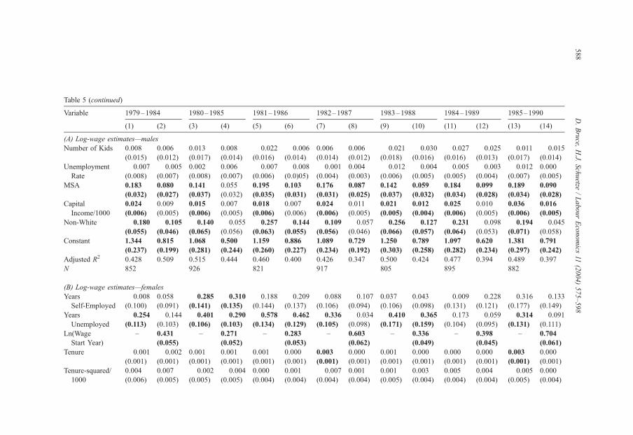
Table 5 (continued)

Variable 1979–1984 1980–1985 1981–1986 1982–1987 1983–1988 1984–1989 1985–1990

(1) (2) (3) (4) (5) (6) (7) (8) (9) (10) (11) (12) (13) (14)

(A) Log-wage estimates—males

Number of Kids 0.008

(0.015)

0.006

(0.012)

0.013

(0.017)

0.008

(0.014)

� 0.022

(0.016)

� 0.006

(0.014)

0.006

(0.014)

0.006

(0.012)

� 0.021

(0.018)

� 0.030

(0.016)

� 0.027

(0.016)

� 0.025

(0.013)

� 0.011

(0.017)

� 0.015

(0.014)

Unemployment

Rate

� 0.007

(0.008)

� 0.005

(0.007)

0.002

(0.008)

0.006

(0.007)

� 0.007

(0.006)

� 0.008

(0.0)05)

� 0.001

(0.004)

0.004

(0.003)

� 0.012

(0.006)

� 0.004

(0.005)

� 0.005

(0.005)

� 0.003

(0.004)

� 0.012

(0.007)

0.000

(0.005)

MSA 0.183

(0.032)

0.080

(0.027)

0.141

(0.037)

0.055

(0.032)

0.195

(0.035)

0.103

(0.031)

0.176

(0.031)

0.087

(0.025)

0.142

(0.037)

0.059

(0.032)

0.184

(0.034)

0.099

(0.028)

0.189

(0.034)

0.090

(0.028)

Capital

Income/1000

0.024

(0.006)

0.009

(0.005)

0.015

(0.006)

0.007

(0.005)

0.018

(0.006)

0.007

(0.006)

0.024

(0.006)

0.011

(0.005)

0.021

(0.005)

0.012

(0.004)

0.025

(0.006)

0.010

(0.005)

0.036

(0.006)

0.016

(0.005)

Non-White � 0.180

(0.055)

� 0.105

(0.046)

� 0.140

(0.065)

� 0.055

(0.056)

� 0.257

(0.063)

� 0.144

(0.055)

� 0.109

(0.056)

� 0.057

(0.046)

� 0.256

(0.066)

� 0.127

(0.057)

� 0.231

(0.064)

� 0.098

(0.053)

� 0.194

(0.071)

� 0.045

(0.058)

Constant 1.344

(0.237)

0.815

(0.199)

1.068

(0.281)

0.500

(0.244)

1.159

(0.260)

0.886

(0.227)

1.089

(0.234)

0.729

(0.192)

1.250

(0.303)

0.789

(0.258)

1.097

(0.282)

0.620

(0.234)

1.381

(0.297)

0.791

(0.242)

Adjusted R2 0.428 0.509 0.515 0.444 0.460 0.400 0.426 0.347 0.500 0.424 0.477 0.394 0.489 0.397

N 852 926 821 917 805 895 882

(B) Log-wage estimates—females

Years

Self-Employed

� 0.008

(0.100)

0.058

(0.091)

� 0.285

(0.141)

� 0.310

(0.135)

� 0.188

(0.144)

� 0.209

(0.137)

� 0.088

(0.106)

� 0.107

(0.094)

0.037

(0.106)

0.043

(0.098)

� 0.009

(0.131)

� 0.228

(0.121)

� 0.316

(0.177)

� 0.133

(0.149)

Years

Unemployed

� 0.254

(0.113)

� 0.144

(0.103)

� 0.401

(0.106)

� 0.290

(0.103)

� 0.578

(0.134)

� 0.462

(0.129)

� 0.336

(0.105)

� 0.034

(0.098)

� 0.410

(0.171)

� 0.365

(0.159)

� 0.173

(0.104)

� 0.059

(0.095)

� 0.314

(0.131)

� 0.091

(0.111)

Ln(Wage

Start Year)

– 0.431

(0.055)

– 0.271

(0.052)

– 0.283

(0.053)

– 0.603

(0.062)

– 0.336

(0.049)

– 0.398

(0.045)

– 0.704

(0.061)

Tenure � 0.001

(0.001)

� 0.002

(0.001)

0.001

(0.001)

0.001

(0.001)

0.001

(0.001)

0.000

(0.001)

0.003

(0.001)

0.000

(0.001)

0.001

(0.001)

0.000

(0.001)

0.000

(0.001)

0.000

(0.001)

0.003

(0.001)

0.000

(0.001)

Tenure-squared/

1000

0.004

(0.006)

0.007

(0.005)

� 0.002

(0.005)

� 0.004

(0.005)

0.000

(0.004)

0.001

(0.004)

� 0.007

(0.004)

0.001

(0.004)

0.001

(0.005)

0.003

(0.004)

0.005

(0.004)

0.004

(0.004)

� 0.005

(0.005)

0.000

(0.004)

D.Bruce,

H.J.

Schuetze

/LabourEconomics

11(2004)575–598

588

Union 0.134

(0.076)

0.042

(0.070)

0.185

(0.083)

0.158

(0.079)

0.104

(0.100)

0.095

(0.095)

� 0.010

(0.080)

� 0.094

(0.071)

0.251

(0.083)

0.164

(0.079)

0.060

(0.087)

0.013

(0.078)

0.093

(0.089)

0.048

(0.075)

Age 0.063

(0.021)

0.041

(0.019)

0.043

(0.022)

0.039

(0.021)

0.089

(0.026)

0.084

(0.024)

0.024

(0.022)

0.014

(0.019)

0.070

(0.025)

0.029

(0.024)

0.084

(0.022)

0.053

(0.020)

0.041

(0.024)

0.003

(0.020)

Age-squared/100 � 0.087

(0.028)

� 0.064

(0.025)

� 0.064

(0.029)

� 0.059

(0.028)

� 0.126

(0.033)

� 0.117

(0.031)

� 0.033

(0.028)

� 0.019

(0.025)

� 0.096

(0.032)

� 0.042

(0.031)

� 0.113

(0.028)

� 0.073

(0.026)

� 0.056

(0.031)

� 0.007

(0.027)

High School

Dropout

� 0.204

(0.072)

� 0.131

(0.066)

� 0.134

(0.087)

� 0.045

(0.085)

� 0.194

(0.099)

� 0.162

(0.094)

� 0.276

(0.085)

� 0.095

(0.077)

� 0.381

(0.090)

� 0.260

(0.086)

� 0.208

(0.083)

� 0.120

(0.076)

� 0.408

(0.115)

� 0.338

(0.096)

Some College 0.157

(0.066)

0.110

(0.060)

0.136

(0.072)

0.139

(0.069)

0.047

(0.081)

0.000

(0.077)

0.008

(0.066)

� 0.012

(0.058)

0.003

(0.067)

� 0.001

(0.062)

0.005

(0.063)

� 0.007

(0.057)

0.047

(0.067)

� 0.059

(0.057)

College Graduate 0.376

(0.076)

0.228

(0.071)

0.404

(0.079)

0.345

(0.077)

0.391

(0.091)

0.264

(0.090)

0.362

(0.078)

0.160

(0.072)

0.191

(0.095)

0.136

(0.089)

0.356

(0.082)

0.254

(0.075)

0.370

(0.082)

0.119

(0.072)

Married 0.043

(0.053)

0.040

(0.048)

0.075

(0.057)

0.084

(0.055)

� 0.002

(0.064)

� 0.037

(0.062)

0.105

(0.055)

� 0.006

(0.048)

0.075

(0.061)

0.067

(0.057)

� 0.022

(0.058)

0.019

(0.053)

0.027

(0.062)

0.034

(0.052)

Number of Kids 0.007

(0.028)

0.012

(0.025)

� 0.013

(0.031)

� 0.019

(0.030)

� 0.011

(0.036)

� 0.020

(0.034)

0.034

(0.033)

0.024

(0.029)

� 0.082

(0.029)

� 0.050

(0.028)

� 0.004

(0.029)

� 0.009

(0.026)

0.013

(0.029)

0.022

(0.024)

Unemployment

Rate

0.015

(0.014)

0.012

(0.013)

� 0.005

(0.014)

� 0.013

(0.013)

0.012

(0.014)

0.009

(0.013)

0.014

(0.008)

0.013

(0.007)

� 0.010

(0.009)

� 0.007

(0.009)

� 0.018

(0.008)

� 0.016

(0.007)

� 0.001

(0.012)

0.002

(0.010)

MSA 0.277

(0.059)

0.138

(0.056)

0.285

(0.068)

0.238

(0.065)

0.293

(0.068)

0.242

(0.066)

0.313

(0.060)

0.129

(0.056)

0.161

(0.058)

0.089

(0.055)

0.233

(0.053)

0.135

(0.049)

0.120

(0.057)

0.004

(0.049)

Capital Income/

1000

0.017

(0.006)

0.014

(0.006)

� 0.005

(0.007)

� 0.009

(0.006)

0.007

(0.012)

0.006

(0.012)

� 0.002

(0.009)

� 0.006

(0.008)

0.004

(0.003)

0.003

(0.003)

0.019

(0.008)

0.010

(0.008)

0.027

(0.011)

0.012

(0.009)

Non-White � 0.227

(0.077)

� 0.147

(0.070)

� 0.152

(0.088)

� 0.122

(0.084)

� 0.055

(0.100)

� 0.032

(0.095)

� 0.266

(0.086)

� 0.117

(0.077)

� 0.148

(0.085)

� 0.077

(0.080)

� 0.206

(0.084)

� 0.097

(0.077)

� 0.426

(0.102)

� 0.163

(0.088)

Constant 0.716

(0.371)

0.587

(0.335)

1.243

(0.404)

0.919

(0.391)

0.377

(0.471)

0.067

(0.452)

1.239

(0.392)

0.599

(0.351)

0.972

(0.459)

1.110

(0.428)

0.870

(0.382)

0.663

(0.345)

1.414

(0.450)

0.912

(0.379)

Adjusted R2 0.402 0.363 0.451 0.431 0.485 0.461 0.462 0.407 0.468 0.435 0.463 0.418 0.482 0.403

N 286 303 274 343 318 357 330

Entries are ordinary least squares regression coefficients with standard errors in parentheses. The dependent variable for each column is the log of average hourly earnings

as of the last endpoint. Bold type indicates statistical significance at the 5% level. Region coefficients were omitted.

D.Bruce,

H.J.

Schuetze

/LabourEconomics

11(2004)575–598

589


continued wage employment. In comparison, an additional year of unemployment is

generally associated with negative relative wage returns that are larger in magnitude

than years of self-employment. An additional year of unemployment is associated with

a wage reduction of 8.2–55.7% upon return to full-time employment relative to a year

of continued wage employment, and the differences are statistically significant in all

but the 1979–1984 time period. As noted above selection may account for the rather

large negative effects estimated here.

In fact, the results presented in the even numbered columns of Table 5A suggest

that men in our samples ‘‘negatively select’’ into both self-employment and unem-

ployment. However, in all cases where the relative returns to self-employment and

unemployment are negative, the magnitudes of the effects are considerably smaller

once we control for unobserved heterogeneity. The estimates of the relative wage loss

from an additional year of self-employment experience in the even number columns

range from 2.8% to 10.8%. This suggests that men who select into self-employment

and unemployment have unobserved characteristics that are associated with poorer

wage sector outcomes than those who remain in the wage sector. Even after accounting

for differences in time invariant unobserved heterogeneity, however, experience in self-

employment still has a smaller negative effect than unemployment experience for men.

In this case, however, these differences are statistically significant in slightly fewer of

the time periods.22

While there are several important differences these general findings also hold for the

females in our sample (Table 5B). For women in our sample, the point estimates on

years of self-employment experience are negative in all but the 1983–1988 time period.

However, likely because of the small sample sizes and a low incidence of self-

employment among women, these point estimates are only statistically significantly

different from zero in the 1980–1985 time period. Much like the results for men, the

coefficients on years of unemployment experience are generally larger, more consistently

negative and statistically significant23 (though only statistically significantly different

from the negative returns to self-employment in the 1983–1988 window). Finally,

comparing the even to odd numbered columns in Table 5B it appears that, unlike men,

women do not negatively select into self-employment but, like men, there is evidence of

negative selection into unemployment.

Coefficients on the remaining variables in Table 5A and B are largely consistent with

earlier findings in the labor economics literature and do not warrant lengthy attention here.

To summarize briefly, wages tend to be higher for those with more tenure on the initial job

and more education as of the initial year. Age exerts the expected hill-shaped effect on

wages, and members of non-White races have lower wages. Residence in an MSA tends to

increase average hourly earnings.

22 In addition to the 1984–1989 time period, when we control for heterogeneity the difference between

the returns to self and unemployment is statistically insignificant in the 1979–1984 and 1983–1988 periods

as well.23 These effects are somewhat larger than those estimated for displaced workers over the same period in

Farber (2001). These differences are likely due to differences in samples, as previously discussed, and in period

length (Farber examines 3-year windows compared to our 5-year windows).


6. Robustness checks

Our first robustness check considers the effect of self-employment experience on

wage-sector earnings over a longer time period. We present two sets of results for 10-

year windows in Table 6: 1979–1989 and 1980–1990. This analysis has the advantage

of allowing for longer spells in self-employment. However, one disadvantage is that we

give up some precision in measuring many of the other exogenous variables in our

model. Recall that we measure characteristics at the initial period. By expanding the

window we increase the probability that some of these characteristics have changed by

the end of the period examined. Table 6 includes only coefficients and standard errors

for the ‘‘Years Self-Employed’’ and ‘‘Years Unemployed’’ variables. For men in our

sample, the results in Table 6 reveal similar patterns to our baseline findings. If

anything, the magnitude of the relative negative wage returns to years of self-

employment appear to be somewhat smaller. Nonetheless, brief self-employment

experience is found to reduce average hourly earnings upon return to the wage sector

relative to a continued spell in wage employment for men. However, the negative

consequences associated with self-employment experience appear to be small relative

to the effects of spells of unemployment. For women in our sample, the results are

mixed. The relative effect of years of self-employment is essentially zero in the 1979–

1989 period but is negative and large relative to the effects of unemployment in the

1980–1990 window. This inconsistency with previous results is likely due to the

further reduction in sample sizes and the loss of precision in measuring exogenous

variables.

Finally, to improve our estimates of the effects of self-employment experience on

wages, we consider the possibility that those who have brief self-employment experience

should actually be compared to those who remain in the wage sector but who also

experience at least one job change during the 5-year window. To investigate this, we

identify wage job changers in the PSID by comparing annual three-digit occupation

codes and omit workers who have the same wage occupation throughout the 5-year

window. Results in Table 7 are similar to our baseline results in Table 5A and B, with

Table 6

Wage regression estimates—10-year time window

Years Males Females

1979–1989

Years Self-Employed � 0.065 (0.015) 0.002 (0.065)

Years Unemployed � 0.202 (0.029) � 0.154 (0.058)

N, Adjusted R2 735, 0.464 230, 0.356

1980–1990

Years Self-Employed � 0.019 (0.018) � 0.273 (0.089)


N, Adjusted R2 735, 0.449 237, 0.218

Entries are ordinary least squares regression coefficients on the ‘‘Years Self-Employed’’ and ‘‘Years

Unemployed’’ variables with standard errors in parentheses. All regressions also include the variables in Table

5 including controls for endogeneity. Bold type indicates statistical significance at the 5% level.

Table 7

Log wage regression estimates—workers who changed jobs at least once

Years Males Females

1979–1984



N, Adjusted R2 843, 0.504 281, 0.463

1980–1985



N, Adjusted R2 915, 0.451 299, 0.318

1981–1986



N, Adjusted R2 577, 0.487 195, 0.343

1982–1987



N, Adjusted R2 624, 0.533 229, 0.374

1983–1988



N, Adjusted R2 554, 0.441 224, 0.418

1984–1989



N, Adjusted R2 600, 0.452 245, 0.325

1985–1990



N, Adjusted R2 605, 0.515 226, 0.592

Entries are ordinary least squares regression coefficients on the ‘‘Years Self-Employed’’ and ‘‘Years

Unemployed’’ variables with standard errors in parentheses. All regressions also include the variables in Table

5 including controls for endogeneity. Bold type indicates statistical significance at the 5% level.


the exception that fewer of the point estimates are statistically significantly different

from zero at the 5% level. The general conclusion that brief self-employment experience

does not increase post-self-employment average hourly earnings continues to hold,

regardless of whether the comparison group includes those who do not change wage

jobs during the period of analysis.24 These results do, however, suggest that the returns

24 We also explored the use of tenure data in the PSID, identifying wage job changers as those whose tenure

on the current job was ever less than 12 months during each 5-year window. While this cost us a substantial

reduction in sample sizes, results were largely similar to those in Table 8.


to self-employment experience are likely closer to zero than our earlier results may

have suggested.

7. Other potential consequences

To this point, we have restricted our attention to the wage consequences of self-

employment experience for workers who return to full-time employment by the end of

each of the 5-year windows. However, there are potentially other labor market conse-

quences associated with short self-employment spells. For instance, it may be difficult for

those workers who fail at self-employment to subsequently find wage employment. In

addition, those who do re-enter the wage sector might only be able to find part-time

employment. We examine these potential consequences in this section.

For consistency, we focus on individuals who are full-time wage employed at the

beginning of each of the 5-year windows and who are not self-employed at the end.

Looking only at those who are wage employed at the end point we examine what effect

any self-employment experience has on the probability of part-time employment. The

upper portion of Table 8 provides raw part-time employment rates among this group. We

Table 8

Percent part-time and unemployed by employment experience

Years Males Females

All

employees

Ever

self-employed

Ever

unemployed

All

employees

Ever

self-employed

Ever

unemployed

Percent of employees part-time at end of period

1979–1984 14.32% 13.41% 50.70% 26.82% 33.33% 31.03%

1980–1985 10.73% 13.68% 29.17% 27.19% 40.00% 47.62%

1981–1986 11.95% 15.00% 29.48% 28.57% 46.15% 53.13%

1982–1987 10.94% 16.22% 35.00% 26.73% 35.29% 51.52%

1983–1988 8.66% 12.24% 47.46% 22.95% 38.46% 50.00%

1984–1989 8.03% 19.04% 22.73% 23.53% 55.00% 36.00%

1985–1990 7.35% 9.43% 21.67% 25.68% 44.44% 35.00%

Percent of workforce unemployed at end of period

1979–1984 2.56% 5.74% 16.71% 2.30% 0.00% 3.33%

1980–1985 3.84% 5.00% 20.00% 2.20% 0.00% 25.00%

1981–1986 4.29% 6.98% 13.33% 1.90% 7.14% 5.88%

1982–1987 2.25% 0.00% 4.76% 1.21% 10.53% 5.71%

1983–1988 2.20% 0.00% 14.49% 1.84% 7.14% 14.29%

1984–1989 1.50% 2.33% 4.35% 1.40% 4.76% 0.00%

1985–1990 1.93% 5.36% 7.69% 2.06% 0.00% 9.09%

Entries are percentages as of the endpoint in the ‘‘Years’’ column for those who were full-time employed at the

start of the period. Sample used in part-time analysis (upper portion of the table) includes only those who were

employed in the wage sector at the endpoint. Sample used in unemployment analysis (lower portion of the table)

excludes those who were self-employed at the endpoint. The columns are defined on the basis of labor market

experience between the endpoints.



compare all individuals in our sample to those with any self-employment experience

between the end points and to those who had any unemployment experience.25 In almost

all cases, the part-time employment rates of men and women who experienced a short spell

of self-employment are higher than the average of the sample. However, the part-time

employment rates of those with self-employment experience are substantially lower than

the group of workers who experienced unemployment in all periods for men and

somewhat lower in many of the periods for women.

In Table 8, we also look at the effects of self-employment on unemployment. The lower

portion of Table 8 gives end period unemployment rates for workers who are labor force

participants at the end of each of the periods by employment experience. Because the

incidence of unemployment in any given year is rare the percentages are not as uniform

across periods. In most cases, the unemployment rates of the ever self-employed groups

are somewhat larger than those for all individuals in the sample. However, as we might

expect, unemployment rates of the ever unemployed do tend to be larger despite these

sample considerations.

To investigate these possible consequences more carefully, we estimate linear

probability models of end-period part-time employment status and unemployment status

by OLS26, separately for men and women. Along with the list of controls regarding the

initial-period characteristics from the previous analysis (including the log of wages, our

proxy variable for productivity), we include an indicator variable which is set equal to 1

if the individual had any self-employment experience between the end points of the 5-

year window.27 Again, for comparison, an indicator variable for unemployment experi-

ence is also included as a regressor. Table 9 contains the coefficient estimates and

heteroskedasticity corrected standard errors for the self-employment and unemployment

experience indicator variables. The results for males (upper portion of table) are

consistent with the raw data. Previous self-employment experience appears to have a

small positive effect on the probability of part-time employment and unemployment at

the end point, but in almost all cases, the effect is not statistically significant. These

results contrast with the relatively large positive effects of unemployment experience on

the probability of subsequent part-time employment and unemployment found using the

same sample.28 Likely due to small sample sizes the results for women are much less

consistent across periods. However, the table provides some evidence that self-employ-

ment experience is associated with an increased probability of subsequent part-time

employment and unemployment, although the coefficient on any unemployment expe-

rience is more frequently positive and significant.

25 Note that some overlap between these two groups is possible.26 We chose the linear probability model over logit or probit for ease in interpreting the coefficients. We

adjust the standard errors for the heteroskedasticity that is inherent in the model using White (1980) estimator. In

any case, we experimented using probit and found qualitatively similar results.27 Our choice of binary indicators for self-employment and unemployment experience in this part of the

analysis is made for convenience of interpretation, as well as the fact that experimentation with more continuous

measures as in our log wage regressions yield qualitatively identical results.28 The coefficients on the unemployment experience indicators are statistically different from those on self-

employment experience in all periods except the 1984–1989 period.

Table 9

Linear probability regression estimates—part-time and unemployment at end of period

Variable 1979–1984 1980–1985 1981–1986 1982–1987 1983–1988 1984–1989 1985–1990

Males

Probability of part-time employment

Any Self-Employment � 0.037 (0.039) 0.019 (0.033) 0.022 (0.038) 0.019 (0.037) 0.004 (0.039) 0.103 (0.042) 0.014 (0.037)

Any Unemployment 0.367 (0.043) 0.173 (0.038) 0.152 (0.040) 0.230 (0.037) 0.392 (0.036) 0.136 (0.035) 0.145 (0.036)

Adjusted R2 0.090 0.030 0.039 0.071 0.155 0.052 0.024

N 1026 1053 937 1042 889 984 960

Probability of unemployment

Any Self-Employment 0.028 (0.017) 0.002 (0.019) 0.021 (0.023) � 0.031 (0.018) � 0.033 (0.021) 0.004 (0.019) 0.039 (0.019)

Any Unemployment 0.134 (0.018) 0.157 (0.021) 0.082 (0.024) 0.023 (0.018) 0.123 (0.018) 0.027 (0.016) 0.063 (0.018)

Adjusted R2 0.069 0.072 0.022 0.006 0.076 0.008 0.011

N 1053 1095 979 1066 909 999 979

Females

Probability of part-time employment

Any Self-Employment 0.059 (0.102) 0.077 (0.105) 0.094 (0.137) 0.086 (0.112) 0.152 (0.119) 0.305 (0.096) 0.186 (0.107)

Any Unemployment � 0.014 (0.089) 0.125 (0.103) 0.264 (0.085) 0.221 (0.082) 0.271 (0.101) 0.091 (0.087) 0.042 (0.101)

Adjusted R2 0.014 0.059 0.052 0.032 0.039 0.063 0.025

N 425 445 413 490 427 493 474

Probability of unemployment

Any Self-Employment � 0.018 (0.034) � 0.048 (0.032) 0.043 (0.041) 0.095 (0.026) 0.070 (0.036) 0.039 (0.027) � 0.013 (0.035)

Any Unemployment � 0.003 (0.030) 0.243 (0.028) 0.042 (0.026) 0.042 (0.019) 0.135 (0.029) � 0.010 (0.025) 0.074 (0.032)

Adjusted R2 0.043 0.162 NA 0.058 0.055 NA 0.021

N 435 455 421 496 435 500 484

Entries are ordinary least squares regression coefficients with White (1980) standard errors in parentheses. The dependent variable in all cases is an indicator variable

(equal to 1 if the worker is part-time employed at the end of the 5-year window in the upper portions of the table and equal to 1 if the worker is unemployed at the end of

the 5-year window in the lower portions of the table). Bold type indicates statistical significance at the 5% level. Additional coefficients were omitted (see text).

D.Bruce,

H.J.

Schuetze

/LabourEconomics

11(2004)575–598

595


8. Conclusions

In theory, prior self-employment experience has the potential to either improve or

worsen (or have no effect on) labor market outcomes for workers who eventually return to

the wage sector. Using regressions of average hourly earnings on a variety of control

variables including controls for time invariant unobserved heterogeneity, we find no

empirical evidence that short self-employment experiences increase wages relative to

continued wage employment for men or women. If any nonzero impact can be discerned

from these data, it is that (compared to wage employment) an additional year of self-

employment might actually reduce post-self-employment earnings in the wage sector by

anywhere from 3% to 11% for men. These results contrast to a certain extent with the

results of previous research by Williams (2000) who found the returns to self-employment

to be positive and equal to the returns to wage employment for men and positive but less

than the returns to wage employment for women. These differences may be due, in part, to

our focus on short-term self-employment as well as the differences in the age distribution

of the sample used in that study which was much younger and less representative of the

overall population than our sample.

Unlike previous researchers, we also examine the effect of short self-employment spells

on future employment prospects. In particular, we estimate the effect that self-employment

experience has on the probabilities of subsequent part-time employment and unemploy-

ment. We find that, relative to wage sector experience, self-employment experience does

not improve and may diminish subsequent employment outcomes. It appears that a short

spell of self-employment may increase the probability of unemployment by anywhere

from 3% to 10%, and part-time employment by 10–30%. These results provide useful

information in terms of evaluating the potential costs and benefits of public policies that

support small business formation. On the surface, efforts to increase entrepreneurial

activity may result in less favorable subsequent consequences in the form of lower

employment probabilities, higher part-time employment probabilities, and lower earnings

upon an eventual return to the wage sector.

Additionally, throughout our analysis, we compare the labor market effects of spells of

self-employment to the effects of spells in unemployment, in part to shed light on the

likely effectiveness of recent self-employment assistance programs focused on preventing

unemployment spells. We find that the negative labor market consequences associated

with unemployment spells in most of the 5-year windows examined are more severe than

those associated with self-employment. Specifically, unemployment experience increases

the probability of subsequent part-time employment by 14–40%, and of subsequent

unemployment by 6–25%. To the extent that our analysis captures the underlying wage

and employment effects of self-employment and unemployment, these results suggest that

certain benefits may arise from programs that promote self-employment as an alternative

to unemployment.

Several caveats are in order, however. First, we have not fully addressed the issue of

selection out of self-employment or unemployment. This may bias our estimates of the

returns to self-employment if those who enter but do not leave self-employment within our

period of analysis are those who would have had higher wages upon returning to the wage

sector. Further, selection out of the self and unemployment states may differ systematically


resulting in our finding of larger negative consequences to unemployment. This would be

the case, for example, if individuals who are self-employed have higher reservation wages

for wage sector reemployment than those who are unemployed. Second, our choice of time

periods, while based on concerns of business cycles and tax changes, may be somewhat

arbitrary. It could be the case that the labor market effects of self-employment and

unemployment are quite different during other periods of time, especially for a window of

time that spans a recession. Finally, despite accounting for wage and employment

consequences, we are not able to assess nonpecuniary costs of self-employment experience

such as the loss of fringe benefits.

Despite all of this, we believe that our results bring to the forefront new issues for

consideration in the evaluation of the likely ‘‘effect’’ of various self-employment

assistance programs. Our results suggest that the effectiveness of such programs depends

to a great extent on which sector of the labor market workers are being attracted from to

become entrepreneurs. Generally, we find that workers who remain in wage sector jobs do

better in terms of wage outcomes than those who experience brief spells of self-

employment but that those with spells of unemployment fare even worse than those with

spells of self-employment. Thus, in evaluating programs aimed at promoting self-

employment among the wage employed, such as those that provide start-up grants or

general tax breaks, policy makers must weigh the possible deleterious effects of spells in

self-employment on wages against the possible positive aspects of such policies. On the

other hand, these results suggest that an evaluation of programs that promote self-

employment among the unemployed should account not only for the promise of reducing

public assistance rolls and creating new jobs but also for the fact that (compared to

unemployment) self-employment may provide workers with an opportunity to maintain

human capital in cases where wage sector employment is not an option.

Acknowledgements

The authors would like to thank Robert Fairlie, Alicia Robb, Matthew Murray, and two

anonymous referees for insightful comments on earlier drafts. We also thank participants at

the APPAM meetings and at seminar series at the University of British Columbia and the

University of Tennessee. Any omissions or errors are solely the responsibility of the authors.

References

Birch, D.L., 1979. Small business—how many jobs? The Brookings Review, Winter, 14–17.

Evans, D.S., Leighton, L.S., 1989. Some empirical aspects of entrepreneurship. American Economic Review 79,

519–535.

Farber, H.S., 2001. Job loss in the United States, 1981–1999. Working Paper No. 453, Princeton University

Industrial Relations Section.

Ferber, M.A., Waldfogel, J., 1998. The long-term consequences of nontraditional employment. Monthly Labor

Review 121, 3–12.

Fuchs, V., 1982. Self-employment and labor force participation of older males. Journal of Human Resources 17,

339–357.


Holtz-Eakin, D., 1995. Should small businesses be tax-favored? National Tax Journal 48, 387–395.

Holtz-Eakin, D., Joulfaian, D., Rosen, H.S., 1994. Sticking it out: entrepreneurial survival and liquidity con-

straints. Journal of Political Economy 102, 53–75.

Holtz-Eakin, D., Rosen, H.S., Weathers, R., 2000. Horatio Alger meets the mobility tables. Small Business

Economics 14, 243–274.

Katz, L.F., Murphy, K., 1992. Changes in relative wages, 1963–87: supply and demand factors. Quarterly

Journal of Economics 107, 35–78.

Taylor, M.P., 1999. Survival of the fittest? An analysis of self-employment duration in Britain. Economic Journal

109, C140–C155.

Uhly, A., 2001 Consequences of transient self-employment for wages. Working Paper. University of Trier.

Vroman, W., 1997. Self-Employment Assistance: Revised Report. The Urban Institute, Washington.

White, H., 1980. A heteroskedasticity-consistent covariance matrix estimator and a direct test for heteroskedas-

ticity. Econometrica 48, 817–830.

Williams, D.R., 2000. Consequences of self-employment for women and men in the United States. Labour

Economics 7, 665–687.

Williams, D.R., in press. Returns to education and experience in self-employment: evidence from Germany,

Journal of Applied Social Science Studies.

Wooldridge, J.M., 2002. Econometric Analysis of Cross Section and Panel Data. MIT Press, Cambridge, MA.

The labor market consequences of experience in self …web.utk.edu/~dbruce/labec04.pdf · aCenter...

Documents

Transcript of The labor market consequences of experience in self …web.utk.edu/~dbruce/labec04.pdf · aCenter...