THE JOURNAL OF RETIREMENT - Pension Research … · THE JOURNAL OF RETIREMENT FALL How Much Should...

T H E J O U R N A L O F

The Voices of Influence | iijournals.com

RETIREMENT FALL 2016 Volume 4 Number 2 www.iijor.com

TH

E JOU

RN

AL O

F RET

IREM

ENT

FALL

How Much Should DC Savers Worry about Expected Returns?ANTTI ILMANEN, MATTHEW RAUSEO, AND LIZA TRUAX

How MucH SHould dc SaverS worry about expected returnS? Fall 2016

Antti ilmAnen

is a principal at AQR Capital Management in London, [email protected]

mAtthew RAuseo

is a vice president at AQR Capital Management in Greenwich, [email protected]

lizA tRuAx

is an associate at AQR Capital Management in Greenwich, [email protected]

How Much Should DC Savers Worry about Expected Returns?Antti ilmAnen, mAtthew RAuseo, And lizA tRuAx

Defined contribution (DC) plans have increasingly become the retirement savings program of choice for corporate sponsors.

As a result, plan sponsors, consultants, and independent researchers have put consid-erable effort into evaluating the expected retirement income these plans may provide. A popular metric used in this assessment is the Retirement Income Replacement Ratio (RR), which is an estimate of the percentage of final income that a participant can expect annually in retirement.1 By most accounts, the average 401(k) participant is not saving enough and will fall short of the income he or she needs in retirement. As a result, much of the research in this space has focused on the impact that savings rates can have on RRs and further, how best to incentivize saving through features such as employer match, automatic enrollment, and automatic escala-tion of contributions.

In this article, we extend the research by exploring the impact that capital market returns can have on RRs. Many RR analyses use stock and bond assumptions anchored on past historical returns; however, these historical returns may not be achievable in the future due to today’s lower starting yields. Surprisingly, although there is gradu-ally growing recognition of lower expected returns in capital markets, the DC literature to date has not quantif ied their impact on

needed savings rates.2 The signs are clear—for a given retirement income target, people need to save more. But how much more? In our analysis, we illustrate how even mod-erate reductions in capital market returns can have an outsized impact on RRs—an impact that might not easily be bridged by simply adjusting savings levels. In light of these results, we advocate that plan sponsors focus on both incentivizing saving and identifying investment solutions that enhance expected returns (with reasonable risk) to help partici-pants reach their retirement goals.

REPLACEMENT RATIO CALCULATION USING HISTORICALLY ANCHORED EXPECTED RETURNS

Saving is clearly an important piece of achieving retirement goals, and it’s also the part that is most directly controlled by a par-ticipant. From this perspective, it makes per-fect sense that plan sponsors typically expend considerable effort on incentivizing savings and view it as the primary path through which participants can achieve their goals. The natural question is then, what level of savings has historically been needed in order to achieve adequate retirement income?

We will start with a simple RR cal-culation to answer this question. For our base-case participant, we assume a target

tHe Journal oF retireMent Fall 2016

retirement income replacement of 75%, around 30% of which may come from income sources outside of retire-ment savings. This leaves a target RR of around 45% coming from the DC plan for our participant.

We assume that the participant’s income grows gradually by a 2% real rate over a 40-year period and that he saves a constant percentage of his income annu-ally. In our first simple example, participant savings are invested in a portfolio of 60% U.S. equities and 40% U.S. bonds (whereas in later examples we introduce a glide path with declining equity weights over time). For capital market returns, we use 7.5% and 2.5% constant annual real return for stocks and bonds, respectively, which yields 5.5% annual real returns at the portfolio level. These figures are loosely based on long-term his-torical results (outlined in Exhibit 1).3

In order to convert the wealth generated by these savings and investments into a quantifiable retirement income stream, we assume the participant purchases a 25-year annuity at retirement. We compare the income from this annuity to the participant’s final employment income to calculate the RR. We believe the assumptions we use are in line with common industry assumptions, and our broad results appear to be robust to different rea-sonable variations we have tried. Yet the specific results we report below (savings rates needed to reach a cer-tain RR) will inevitably depend on the assumptions we make regarding the target DC savings component and the other income component of the RR, wage growth, the lengths of working/saving and retirement periods, as well as investment choices and assumed investment

returns over the working/saving and retirement periods. We now turn to a further motivation of our assumptions and to a very brief discussion of the literature.

Target RR in Retirement. The literature offers a range of values for this level, centered around 70%–90%—balancing the likely lower cost of housing, lower work-related expenditure, less need for saving, and reduced spending on dependents with the potentially higher cost of health care.4 We select 75% as a reasonable point estimate.

Replacement of Income from Other Sources. As with targeted RR, the numbers quoted in the literature vary widely, depending on the source and the savers’ financial situation, especially when it comes to “other income.” Other sources include Social Security, home ownership (for its housing services as well as possible reverse mortgages), as well as investments other than DC plan savings. We (must) use one plausible set of inputs, and 30% is in line with earlier research.5

Wage Growth. We assume a constant 2% real wage growth. This includes both the general growth in real wages in the population over time and the growth in wages people earn as they age and gain more experience.

Annuity Rate. We assume that the participant purchases a 25-year period-certain annuity6 which offers a 2% spread over our bond return assumption, based on historical observations. Note that this premium over bonds ref lects both the return on the participants contributed capital and the risk of losing the invested capital in case of early death (in the case of bonds the participant can get the principal back, but with this annuity choice the principal is lost).7 This choice was made for convenience; we looked into other options for retirement investment, such as purchasing a life annuity or continuing to invest in a conservative asset allocation, but found that the results were quite similar when run with the assumptions outlined herein. Ultimately, all the investment options are long-duration assets whose expected returns should move broadly with assumed long-term riskless yields. Thus, our big-picture results should be reasonably robust to other assumptions regarding retirement investment choices.

Using the methodology we have outlined, we esti-mate our base-case participant would have needed to save 8% to reach a 75% total RR. For reference, the cur-rent average participant contribution in U.S. DC plans is around 6%, with an additional 3% average sponsor contribution for employees lucky enough to be offered

e x h i b i t 1Traditional Assets and 60/40 Portfolio Historical Returns through December 2015

Notes: S&P 500 is the Ibbotson Stocks, Bonds, Bills, and Inf lation (SBBI) series U.S. Large Stock TR USD. U.S. 10-year bonds provided by GFD prior to 1980 and Datastream thereafter. U.S. 60/40 is 60% S&P, 40% U.S. 10-year bonds, rebalanced monthly. Returns are excess of CPI. Time periods are chosen to represent a savings and retirement period (~65 years) and a savings-only period (~40 years).

Source: Morningstar, Global Financial Data (GFD), Datastream, AQR.


an employer match.8 It seems reasonable that, at least among those who have a sponsor match to the level of 2% to 3%, the average participant could achieve a 75% RR if historical return assumptions hold true. (All required savings rates quoted in this article include any sponsor match.)

“Exchange Rate” between Expected Returns and Savings Rates

But what if prospective investment returns are not the same as they have been in the past? What if they are lower? How would that impact the amount participants would need to save—is it as simple as a one-for-one trade-off? It turns out the answer to this last question is no: Capital market returns have an outsized impact on savings needs.

Exhibit 2 shows the required savings rate at var-ious real return assumptions. We will focus primarily on Scenarios 2 and 4 for the remainder of the article, but we include all five scenarios here to illustrate the “exchange rate,” or trade-off, between a 1% reduction in investment returns and additional savings needed to achieve a 75% RR. We see that a 1% reduction in annual portfolio return expectations from 5.5% to 4.5% requires 3% additional annual savings to get back to a 75% RR. More broadly, using this simple framework, the exchange rate varies from 2% to 5% additional sav-ings needed for each 1% cut in investment returns. The effect is nonlinear, with larger required savings increases the lower the expected returns.9

One intuition as to why a 1% change in investment return has a larger impact on RR than a 1% change in the

savings rate is that the accumulated investment portfolio is much larger than the annual income. So to compensate for a 1% reduction in investment return, saving must be increased by a larger percentage of annual income. Although these are just estimates, the main takeaway is that in order to compensate for lower capital market returns, participants would have to save meaningfully more to achieve the same goal. If the market does not do as good a job of delivering retirement security as in the past, you must do more yourself.

Current State of Expected Returns

We believe the current state of expected returns highlights the critical importance of the asset alloca-tion and investment decisions that plan sponsors are making. This is particularly important today as cur-rent yields on stocks and bonds put us in a world where Scenario 4’s U.S. 60/40 return expectations in Exhibit 2 are closer to reality than those of Scenario 2 (history-anchored results).

Anchoring projections too much on historical results may present a picture that is far too rosy for current and future savings cohorts. Past market returns were high partly because starting yields for both stocks and bonds were higher; in other words, the assets were cheaper versus fundamentals than they are today. More-over, stocks and bonds became more expensive over time thanks to falling yields and rising valuation multiples, giving windfall gains to investors.10

Compared to historical averages, today we are in a world of lower expected returns. Referencing cur-rent yields, we estimate 4% prospective real return for

e x h i b i t 2“Exchange Rate” Between Savings and Capital Market Assumptions at Various Levels

Notes: U.S. equities are the SBBI series U.S. Large Stock TR USD. U.S. bonds are 10-year bonds provided by GFD prior to 1980 and Datastream thereafter. U.S. 60/40 is 60% U.S. equities and 40% U.S. 10-year bonds, rebalanced monthly. Returns are excess of CPI. We show savings rates only in full percentage points to avoid false precision of our estimates.

Source: AQR, Morningstar, GFD, Datastream, calculated using the assumptions laid out in this section.


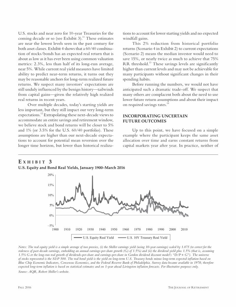
U.S. stocks and near zero for 10-year Treasuries for the coming decade or so (see Exhibit 3).11 These estimates are near the lowest levels seen in the past century for both asset classes. Exhibit 4 shows that a 60/40 combina-tion of stocks/bonds has an expected real return that is about as low as it has ever been using common valuation metrics: 2.3%, less than half of its long-run average, near 5%. While current real yield measures have limited ability to predict near-term returns, it turns out they may be reasonable anchors for long-term realized future returns. We suspect many investors’ expectations are still unduly inf luenced by the benign history—tailwinds from capital gains—given the relatively high realized real returns in recent years.

Over multiple decades, today’s starting yields are less important, but they still impact our very long-term expectations.12 Extrapolating these next-decade views to accommodate an entire savings and retirement window, we believe stock and bond returns will be closer to 5% and 1% (or 3.5% for the U.S. 60/40 portfolio). These assumptions are higher than our next-decade expecta-tions to account for potential mean reversion over the longer time horizon, but lower than historical realiza-

tions to account for lower starting yields and no expected windfall gains.

This 2% reduction from historical portfolio returns (Scenario 4 in Exhibit 2) to current expectations (Scenario 2) means the median investor would need to save 15%, or nearly twice as much to achieve that 75% RR threshold.13 These savings levels are significantly higher than current levels and may not be achievable for many participants without significant changes in their spending habits.

Before running the numbers, we would not have anticipated such a dramatic trade-off. We suspect that many others are complacent both about the need to use lower future return assumptions and about their impact on required savings rates.14

INCORPORATING UNCERTAIN FUTURE OUTCOMES

Up to this point, we have focused on a simple example where the participant keeps the same asset allocation over time and earns constant returns from capital markets year after year. In practice, neither of

e x h i b i t 3U.S. Equity and Bond Real Yields, January 1900–March 2016

Notes: The real equity yield is a simple average of two proxies, (i) the Shiller earnings yield (using 10-year earnings) scaled by 1.075 (to correct for the staleness of past-decade earnings, embedding an annual earnings-per-share growth (G) of 1.5%) and (ii) the dividend yield plus 1.5% (that is, assuming 1.5% G or the long-run real growth of dividends-per-share and earnings-per-share in Gordon dividend discount model’s “D/P + G”). The universe of stocks represented is the S&P 500. The real bond yield is the yield on long-term U.S. Treasury bonds minus long-term expected inf lation based on Blue Chip Economic Indicators, Consensus Economics, and the Federal Reserve Bank of Philadelphia. Survey data became available in 1978; therefore expected long-term inf lation is based on statistical estimates and on 1-year ahead Livingston inf lation forecasts. For illustrative purposes only.

Source: AQR, Robert Shiller’s website.


these is ref lective of how retirement investing works in the real world.

On the asset allocation side, participants in U.S. target-date funds typically start out with aggressive portfolios that are almost entirely invested in equities and then scale that asset allocation to a more conserva-tive portfolio as retirement approaches. On the returns side, the average historical returns mask periods of strong performance and extreme market turmoil. The order in which returns are earned and the timing of favorable and unfavorable market environments can materially impact retirement wealth. These risks are not captured in our original framework. On a related note, in our first example we could only discuss what participants need to save on average to reach their goals. Investors who want to be prepared for the case that they get “unlucky” (in the sense that capital markets deliver realized returns below expectations during their investment lifetime) would need to save even more to ensure a 75% RR. The savings rate could also vary from year to year to accommodate particular expen-diture patterns.

To account for these real-world considerations, we now switch to a more sophisticated framework for calculating replacement ratios. In this approach, rather than assuming a constant U.S. 60/40 portfolio, we incorporate a “glide path” asset allocation between

U.S. stocks and bonds starting at 90% stocks/10% bonds and gliding linearly to 50% stocks/50% bonds at retirement.15

Additionally, instead of assuming constant monthly returns, we simulate the randomness of future market outcomes.16 This allows us to get a sense of what the distribution of outcomes might be—meaning that for a given set of assumptions we can gain insight not only into the typical investor’s savings needs, but also into what those needs might look like for those cohorts that get “lucky” (defined as landing in the 80th percentile of outcomes) or “unlucky” (the 20th percentile of out-comes) for a given set of return expectations.

For this analysis, we focus on Scenario 2 (histori-cally anchored real returns of 7.5% for stocks and 2.5% for bonds) and Scenario 4 (current yield-anchored real returns of 5% for stocks and 1% for bonds). In both sce-narios, we assume annual volatilities of 15% for equities and 5% for bonds. All other assumptions remain the same as in our base case above.

The results of this simulation are shown in Exhibit 5. Focusing f irst on Scenario 2, we see that the median investor would need to save 8% to achieve a 75% RR.17 Saving 6% gets to a 75% RR only in the case that future average returns are similar to his-torical returns and that a cohort gets lucky on top of that. Cohorts that get unlucky and end in the bottom

e x h i b i t 4Expected Real Return of U.S. 60/40 Stock/Bond Portfolio, January 1900–March 2016

Notes: U.S. 60/40 is 60% U.S. real equity yield and 40% real bond yield. The method of estimating expected real returns for each asset class is described in notes to Exhibit 3. For illustrative purposes only.

Source: AQR, Robert Shiller’s website.


quintile of the distribution would need to save closer to 12% to hit a 75% RR.

In the unlucky case, the average participant saving 6% and getting a sponsor match of 3% may be able to get there using some of the same education and savings incentives as noted earlier, but it could still be difficult for those participants to increase their personal contribu-tions by 50%. For those without a sponsor contribution, it would take some meaningful lifestyle adjustments to double their savings in order to reach their retirement goals. Thus, even in the case that capital market expecta-tions do match historical returns, a cohort that just gets unlucky may need to consider additional options outside of just increasing savings to reach their goals.

Switching to Scenario 4, which uses returns assumptions that we would argue are more realistic, we see even more troubling results. In this case, even the lucky cohorts would require a 12% savings (twice the current average) to achieve a 75% RR. Those cohorts that get unlucky with these lower long-term average

assumptions would need to save 20% to get to a 75% RR—a level we expect could be challenging for most participants to achieve.

To summarize, if expected returns are high (anchored loosely on historical experience), the typical (median) outcome requires 8% annual savings rate to reach a 75% RR. If retirement savers want to be conser-vative and increase their chances of achieving that 75% RR even in a bad future capital market scenario, their savings rate needs to be 12%. The numbers get worse if expected returns are low (anchored loosely on cur-rent market yields). Then the typical outcome requires a 15% savings rate, and to insure against a doubly bad experience (low expected returns and a bad draw of even lower future realizations), a 20% savings rate is needed to reach the 75% RR target.18

PARTICIPANTS CAN SAVE MORE OR TRY TO ENHANCE RETURNS (OR BETTER YET, DO BOTH)

What options do participants and plan sponsors have in the face of future lower returns? We believe the best approach to addressing lower capital market expec-tations is likely to be through a combination of saving more and investing more wisely. With the assumptions we have laid out, a 15% savings rate (20% for investors worried about getting unlucky) will put participants in a much better position to reach their goals than the cur-rent average savings of 6%. Initiatives such as matching incentives, automatic enrollment, and automatic escala-tion of contributions have already gone a long way in improving participation and savings rates. Continuing with these measures would certainly improve the odds of achieving adequate retirement income. However, it could be quite difficult for participants who are saving at or below the average rate (and maybe even for those well above the average) to make such a drastic change in savings behavior. One other option is of course working longer (health and other factors permit-ting), which can be seen as a way to save more (with the added—if questionable—benefit of shortening the retirement period).

Another option participants and plan sponsors have is to modify their investment plan to boost expected returns. To achieve this, participants should consider casting a wider net among liquid asset classes across three separate layers: traditional markets, alternatives,

e x h i b i t 5Savings Needed to Reach 75% RR at Various Outcomes

Notes: Replacement ratios are calculated using the methodology described. Scenario 2 returns are sampled monthly throughout the glide path from a distribution that assumes average annual returns of 7.5% for equities and 2.5% for bonds. Scenario 4 assumes average annual returns of 5% for equities and 1% for bonds. “Lucky” corresponds to the 80th percentile across 1,000 simulations, “Median” corresponds to the 50th percentile, and “Unlucky” corresponds to the 20th percentile. Lucky, Median, and Unlucky realized annual portfolio real returns are ~6%, ~5%, ~4%, respectively, for Scenario 2 and ~5%, ~3%, ~2%, respectively, for Scenario 4. For illustrative purposes only.

Source: AQR.


and potentially alpha. (Illiquid private investments are a further possibility for return enhancement but their high costs and opacity raise the bar for including them into DC plans.)

• The bottom layer could incorporate all the major asset-class return premia in the market—traditional equities and bonds, but also credit and commodi-ties, which are typically underrepresented but diversifying to the traditional asset classes.19

• In the middle layer, participants could expand into alternative investments including factor or style premia such as value, momentum, and quality, or classic hedge fund strategies such as managed futures or global macro. Factor premia can be har-vested either through long-only portfolio tilts or long/short strategies. They are best known in stock selection, where cheap stocks, past-year winners, and high-quality stocks have tended to outperform the market in the long run, but the ideas travel well to other asset classes.20 These alternative return sources can be systematically implemented, easily identified, and many come at reasonable fees.

• The top layer is true alpha, the portion of return that is derived from idiosyncratic investment pro-cesses. While adding alpha to a portfolio could certainly enhance returns, it is very challenging to identify in advance those managers that can pro-vide it on a consistent basis net of fees. We discuss these and other return enhancement ideas among liquid assets further in other research.21

Finally, market timing is highly unreliable. Even though virtually “everything appears expensive” (in the sense of having lower expected returns than own past experience), moving all-in to cash would be problematic because the next crash might not come soon enough and most contrarian investors would not have patience to wait for it. Contrarian market timing signals are simply too crude—they tend to trigger action too early—to be useful for most investors.

CONCLUSION

Many DC plan sponsors assume that future long-term capital market returns will be similar to those observed in the benign recent decades. Unfortunately, current market yields may give a more realistic anchor

to future returns, and we quantify that an approximately 2% decline in expected returns would raise the required savings rate from 8% to 15% (to reach 75% RR in the typical outcome).

Although saving more is one part of the answer to the challenge of lower expected returns, there are limits to DC plan participants’ ability and willingness to save more. Apart from true budget constraints, it may be hard to motivate people to save more when rewards for it are more meager than in the past, but that is exactly what is needed to reach a given RR goal. Improving investment returns is another part of the solution. We outline some possible return-enhancing solutions and direct readers to other AQR papers for more extensive discussions on this topic.

A p p e n d i x

REPLACEMENT RATIOS AT DIFFERENT SAVINGS RATES

For readers who prefer to view the problem through the lens of savings rates rather than RRs, we have pro-vided Exhibits A1 and A2 below. In the article, we focus on adjusting the savings level needed to achieve a 75% RR. In this appendix, we show instead what level of RR is achieved

e x h i b i t A 1Median and Bottom Quintile RRs with Historically Anchored Expected Returns

Notes: Median and Unlucky replacement ratio is calculated using the methodology described herein. Exhibit A1 returns sampled monthly from a distribution that assumes average 7.5% annual real returns for equities and 2.5% average annual real returns for bonds. For illustrative purposes only.

Source: AQR.


at various common savings rates for both the historically anchored and the current-yield anchored expected return scenarios.

ENDNOTES

We thank Larry Siegel, Rodney Sullivan, Dan Villalon, Jeff Dunn, and the editor for helpful comments, and we are especially grateful to Robert Capone for the many discussions and guidance in writing this article.

The views and opinions expressed herein are those of the author and do not necessarily ref lect the views of AQR Capital Management, LLC (“AQR”), its affiliates, or its employees. This document does not represent valuation judgments, investment advice, or research with respect to any financial instrument, issuer, security, or sector that may be described or referenced herein and does not represent a formal or official view of AQR.

1For example, if a participant’s f inal annual salary is $60,000, he would need an annual retirement income of $30,000 for a 50% RR. The next section discusses RRs fur-ther, including methods for estimating them and the under-lying assumptions used herein.

2Savers need to offset lower expected returns with greater savings to reach a given retirement target. This is also a key explanation as to why aggressive monetary policy stimulus (including negative real rates and sometimes even

negative nominal rates) has had a surprisingly muted impact on private consumption.

3Here is some detail on why we use the historical geo-metric mean (GM) of returns to anchor our simulation input. If we knew the true arithmetic mean (AM), we would use it, but since we can only estimate AM, it is arguably better to use the GM. Jacquier, Kane, and Marcus [2003] show that the historical AM would give upward-biased estimates of future wealth and that the impact of estimation errors increases with horizon, and they recommend the use of AM for short hori-zons and the use of GM for long horizons where the forecast horizon broadly matches the historical estimation period, as it does in our case. Note that Exhibit 1 contains GM returns over 40-year and 65-year histories, corresponding to a 40-year retirement saving period and a 65-year period that also includes the expected retirement window assumed in our study.

4See Munnell, Webb, and Hou [2014]; Ellement and Lucas [2007]; Palmer, Destafano, and Bone [2008]; and Purcell [2012]. Scholz and Seshadri [2009] criticize the use of RRs as too simple and offer a life-cycle model as a fuller if computationally more demanding alternative. (For example, those with greater expected longevity should have a higher RR, while those whose expenses fall sharply with retirement, such as parents who no longer need to spend on children’s education, can have a lower RR).

5As with targeted RR, the numbers quoted in the literature vary widely, depending on the source and the savers’ financial situation, especially when it comes to “other income.” We (must) use one plausible set of inputs, and 30% is approximately in line with much research, including that of Munnell, Webb, and Hou [2014]; Ellement and Lucas [2007]; and Butrica, Smith, and Iams [2012]. We are agnostic as to where the 30% comes from and note that housing wealth is typically not included as part of retirement wealth, so its treatment in RR calculations is debatable.

6There are advantages and disadvantages to this approach—the advantage is a certain income stream for 25 years (putting aside any potential counterparty risks and inf lation risks), and the disadvantages are the risk of losing the capital in the case of early death and, worst, the risk of outliving the 25-year income stream. Working longer may be a natural early answer to the longevity challenge, but is not an option well into retirement. Life annuities or deferred annuities seem like the best investment answer, yet few DC pension savers have embraced these products.

7Based on average spread of annuities tracked on imme-diateannuities.com from July 2009 to February 2016. Spread is calculated relative to Barclays U.S. Corporate Bond Index. Note that this premium ref lects the loss of capital in case of early death and includes return of the investor’s own con-tributed capital.

e x h i b i t A 2Median and Bottom Quintile RRs With Current Yield-Anchored Expected Returns

Notes: Median and Unlucky replacement ratio calculated using the meth-odology described herein. Exhibit A2 returns are sampled monthly from a distribution that assumes average 5% annual real returns for equities and 1% average annual real returns for bonds. For illustrative purposes only.

Source: AQR.


8Source: Cerulli Retirement Markets Report 2015. It is important to recognize that these figures are only relevant for those individuals whose companies offer a plan and for those employees who have opted to participate. The national numbers would be far lower; however, for this article, we will focus on the subset of employees who have opted into a plan offered to them.

9This table of “exchange rates” between returns and required savings rates can be used in at least three ways (we cover all of them in this article). First and foremost, it tells how much higher savings rates are needed to reach 75% RR if expected market returns are lower today than in the past. (One reason for the large nonlinear effect is that our lower return estimates impact both the accumulation and retirement periods). Second, it gives the cost of insuring against unlucky outcomes in future capital market realizations, in terms of additional savings needed. Third, it shows the benefit of any investment strategies that can enhance future expected returns, in terms of lesser savings needed. For illustrative purposes only.

10For example, the 10-year Treasury had a (nominal) yield just below 8% in 1976 compared to just below 2% in the beginning of 2016. This 6% total yield fall implies an average annual yield fall near 0.15%, which means more than 1% annual capital gains (based on a simple duration approxima-tion). This in-sample richening boosted realized bond returns since 1976, and we can safely assume that it won’t be repeated in the coming decades (as it would require nominal bond yields to drop into a deeply negative territory). A similar, if less extreme, richening benefited U.S. equities, whose Shiller earnings yields and dividend yields roughly halved over the same 40-year period.

11See AQR Capital Management [2016] as well as Asness and Ilmanen [2012]. This is just one way to estimate expected returns, but any approaches based on market yields should tell a broadly comparable story of lower expected returns.

12Whether the coming decades are characterized by sharp corrections in traditional assets or a prolonged period of low yields, our expectations are lower for the next 40 to 65 years than they were for the last 40 to 65 years.

13For robustness, we also considered a 75% target RR where the “income from pension investments” and “other income” each contributed 37.5% (versus 45% and 30%, respectively). In this case, the historically anchored capital market assumptions required ~7% savings, and the current market yield anchored assumptions required ~13% savings—again nearly doubling.

14The challenge from lower expected returns has not been widely appreciated because the windfall gains from falling equity and bond yields has cushioned realized market returns to date, and the practice of extrapolating past long-term returns to assess future expected returns remains too widespread. The impact on savings rates is not widely

appreciated because the numerical exercise we conduct here has rarely been done in public (as far as we know).

15This is broadly consistent with glide paths in the target-date fund industry. See Dhillon, Ilmanen, and Liew [2016].

16We do this by sampling monthly “stock” and “bond” returns from normal distributions each month over the 40-year savings period. In this way, we can create a return stream that is drawn from the same volatility and return distribution as our estimates, but more closely ref lects the risks that investors actually face. We then study the outcomes across 1,000 iterations of these simulated return streams. The distribution captures the uncertainty of returns around the expected values.

17It turns out that the results are close to those of a stable 60/40 portfolio, as described in Exhibit 1, perhaps because the glide path implies on average something close to a 60/40 portfolio (when we recognize that the pension savings pot is largest when the retirement is approaching and the equity weight is edging toward 50%). More generally, because we assume lower expected returns for both stocks and bonds, the assumed shape of the glide path—f lat during the accu-mulation period as in Exhibit 2, or declining with age as in Exhibit 5, or even rising with age—should not change our broad conclusions.

18The appendix provides additional exhibits that show the range of RRs achieved at common savings levels for both the median and the bottom quintile.

19Described by Asness and Ilmanen [2012].20See, for example, Asness, Pedersen, and Moskowitz

[2013] and Asness et al. [2015]. 21See Asness and Ilmanen [2012], Ilmanen et al. [2016]

as well as Dhillon, Ilmanen, and Liew [2016].

REFERENCES

Asness, C., and A. Ilmanen. “The 5 Percent Solution.” Institutional Investor, 2012.

Asness, C., A. Ilmanen, R. Israel, and T. Moskowitz. “Investing With Style.” The Journal of Investment Management, Vol. 13, No. 1 (2015).

Asness, C., L.H. Pedersen, and T. Moskowitz. “Value and Momentum Everywhere.” The Journal of Finance, Vol. 68, No. 3 (2013), pp. 929-985.

AQR Capital Management. “Capital Market Assumptions for Major Asset Classes.” Alternative Thinking, First Quarter, 2016.

Butrica, B., K. Smith, and H. Iams. “This Is Not Your Par-ent’s Retirement: Comparing Retirement Income across Generations.” Social Security Bulletin, Vol. 72, No. 1 (2012).


Dhillon, J., A. Ilmanen, and J. Liew. “Balancing on the Lifecycle: Target-Date Funds Need Better Diversification.” The Journal of Portfolio Management, Vol. 42, No. 4 (2016), pp. 12-27.

Ellement, J., and L. Lucas. “A Retirement Adequacy Analysis of Default Options and Lifecycle Funds.” Benefits Quarterly, 2007.

Ilmanen, A., D. Kabiller, L. Siegel, and R. Sullivan. “The Evolution of DC Plans: Part I.” AQR Whitepaper, 2016.

Jacquier, E., A. Kane, and A. Marcus. “Geometric or Arith-metic Mean: A Reconsideration.” Financial Analysts Journal, Vol. 59, No. 6 (2003), pp. 46-53.

Munnell, A., A. Webb, and W. Hou. “How Much Should People Save?” Center for Retirement Research at Boston College, Number 14-11, 2014.

Palmer, P., R. Destafano, and C. Bone. “2008 Replacement Ratio Study: A Measurement Tool for Retirement Planning.” Aon Hewitt, 2008.

Purcell, P. “Income Replacement Ratios in the Health and Retirement Study,” Social Security Bulletin, Vol. 72, No. 3 (2012).

Scholz, J., and A. Seshadri. “What Replacement Rates Should Households Use?” University of Michigan Retire-ment Research Center, Working Paper, 2009.

To order reprints of this article, please contact Dewey Palmieri at [email protected] or 212-224-3675.

THE JOURNAL OF RETIREMENT - Pension Research … · THE JOURNAL OF RETIREMENT FALL How Much Should...

Documents

Transcript of THE JOURNAL OF RETIREMENT - Pension Research … · THE JOURNAL OF RETIREMENT FALL How Much Should...