The Journal of Financial Perspectives - ey.com · portfolio construction method based on MPT, known...

The Journal of

FinancialPerspectivesEY Global Financial Services Institute November 2014 | Volume 2 – Issue 3

The EY Global Financial Services Institute brings together world-renowned thought leaders and practitioners from top-tier academic institutions, global financial services firms, public policy organizations and regulators to develop solutions to the most pertinentissues facing the financial services industry.

The Journal of Financial Perspectives aims to become the medium of choice for senior financial services executives from banking and capital markets, wealth and asset management and insurance, as well as academics and policymakers who wish to keep abreast of the latest ideas from some of the world’s foremost thought leadersin financial services. To achieve this objective, a board comprising leading academic scholars and respected financial executives has been established to solicit articlesthat not only make genuine contributions to the most important topics, but are also practical in their focus. The Journal will be published three times a year.

gfsi.ey.com

The articles, information and reports (the articles) contained within The Journal are generic and represent the views and opinions of their authors. The articles produced by authors external to EY do not necessarily represent the views or opinions of EYGM Limited nor any other member of the global EY organization. The articles produced by EY contain general commentary and do not contain tailored specific advice and should not be regarded as comprehensive or sufficient for making decisions, nor should be used in place of professional advice. Accordingly, neither EYGM Limited nor any other member of the global EY organization accepts responsibility for loss arising from any action taken or not taken by those receiving The Journal.

http://gfsi.ey.com

EditorialEditor

Shahin ShojaiEY, U.A.E.

Advisory Editors

Dai BedfordEY, U.K.

Michael LeeEY, U.S.

Shaun CrawfordEY, U.K.

David GittlesonEY, U.K.

Carmine DiSibioEY, U.S.

Bill SchlichEY, U.S.

Special Advisory Editors

H. Rodgin CohenSullivan & Cromwell LLP

J. B. Mark MobiusFranklin Templeton

John A. FraserUBS AG

Clare WoodmanMorgan Stanley

Editorial Board

Emilios AvgouleasUniversity of Edinburgh

Deborah J. LucasMassachusetts Institute of Technology

John ArmourUniversity of Oxford

Massimo MassaINSEAD

Tom BakerUniversity of Pennsylvania Law School

Patricia A. McCoyUniversity of Connecticut School of Law

Philip BoothCass Business School and IEA

Tim MorrisUniversity of Oxford

José Manuel CampaIESE Business School

John M. MulveyPrinceton University

Kalok ChanHong Kong University of Science and Technology

Richard D. PhillipsGeorgia State University

J. David CumminsTemple University

Patrice PoncetESSEC Business School

Allen FerrellHarvard Law School

Michael R. PowersTsinghua University

Thierry FoucaultHEC Paris

Andreas RichterLudwig-Maximilians-Universitaet

Roland FüssUniversity of St. Gallen

Philip RawlingsQueen Mary, University of London

Giampaolo GabbiSDA Bocconi

Roberta RomanoYale Law School

Boris GroysbergHarvard Business School

Hato SchmeiserUniversity of St. Gallen

Scott E. HarringtonThe Wharton School

Peter SwanUniversity of New South Wales

Paul M. HealyHarvard Business School

Paola Musile TanziSDA Bocconi

Jun-Koo KangNanyang Business School

Marno VerbeekErasmus University

Takao KobayashiAoyama Gakuin University

Ingo WalterNew York University

Howard KunreutherThe Wharton School

Bernard YeungNational University of Singapore

Executive summaries

The unique risks of portfolio leverage: why modern portfolio theory fails and how to fix itby Bruce I. Jacobs, Principal, Jacobs Levy Equity Management and Kenneth N. Levy,Principal, Jacobs Levy Equity Management

Leverage entails a unique set of risks, such as margin calls, which can forceinvestors to liquidate securities at adverse prices. Modern Portfolio Theory (MPT)fails to account for these unique risks. Investors often use portfolio optimizationwith a leverage constraint to mitigate the risks of leverage, but MPT providesno guidance as to where to set the leverage constraint. We propose an amendedapproach to MPT that allows leverage to be incorporated more effectively. This isachieved by explicitly incorporating a term for investor leverage aversion, as well asvolatility aversion, allowing each investor to determine the right amount of leveragegiven that investor’s preferred trade-offs between expected return, volatility riskand leverage risk. Incorporating leverage aversion into the portfolio optimizationprocess produces portfolios that better reflect investor preferences. Furthermore, to the extent that portfolio leverage levels are reduced, systemic risk in the financialsystem may also be reduced.

https://twitter.com/intent/tweet?text=EY+GFSI+-+The+Journal+of+Financial+Perspectives&url=https%3A%2F%2Fwww.gfsi.ey.com%2Fthe-journal-x.php%3Fpid%3D10%26id%3D73%23.VJlnlQNH8TU.twitter&related=

http://www.facebook.com/sharer/sharer.php?u=https://www.gfsi.ey.com/the-journal-x.php?pid=10%26id=73

http://www.linkedin.com/shareArticle?mini=true&url=https://www.gfsi.ey.com/the-journal-x.php?pid=10%26id=73

https://www.gfsi.ey.com/the-journal-x.php?pid=10&id=73&loc=EmailArticle

1 This article is based on a presentation given at a conference of the Jacobs Levy Equity Management Center for Quantitative Financial Research of the Wharton School, held in New York City, 23 October 2013. Slides and video of the talk, entitled “Leverage aversion — a third dimension in portfolio theory and practice,” are available at: http://jacobslevycenter.wharton.upenn.edu/conference/forum-2013/ The authors thank Judy Kimball and David Landis for their editorial assistance.

AbstractLeverage entails a unique set of risks, such as margin calls, which can force investors toliquidate securities at adverse prices. Modern Portfolio Theory (MPT) fails to account forthese unique risks. Investors often use portfolio optimization with a leverage constraint to mitigate the risks of leverage, but MPT provides no guidance as to where to set the leverage constraint. Fortunately, MPT can be fixed by explicitly incorporating a term for investor leverage aversion, as well as volatility aversion, allowing each investor to determine the right amount of leverage given that investor’s preferred trade-offs between expected return, volatility risk and leverage risk. Incorporating leverage aversion into the portfolio optimization process produces portfolios that better reflect investor preferences. Furthermore, to the extent that portfolio leverage levels are reduced, systemic risk in the financial system may also be reduced.

The unique risks of portfolio leverage: why modern portfolio theory fails and how to fix it1

Bruce I. JacobsPrincipal, Jacobs Levy Equity ManagementKenneth N. LevyPrincipal, Jacobs Levy Equity Management





Modern Portfolio Theory (MPT) asserts that investors prefer portfolios with higher expected returns and lower volatility. Holding a diversified set of assets generally lowers volatility because the price movements of individual assets within a portfolio are partially offsetting; as the price of one security declines, for example, the price of another may rise. As a result, the value of the portfolio tends to vary less than the volatility of its individual assets would suggest.

When Harry Markowitz first advanced this theory in 1952, leverage — that is, borrowing — was not commonly used in investment portfolios [Markowitz (1952) and Markowitz(1959)]. Since then, we have witnessed the rising popularity of instruments that allow high levels of portfolio leverage, such as structured finance products, futures and options. We have also seen increased borrowing of securities to effect short sales2 and borrowing of cash to purchase securities [Jacobs and Levy (2013a)].

A portfolio with leverage differs in a fundamental way from a portfolio without leverage. Consider two portfolios having the same expected return and volatility. One uses leverage while the other is unleveraged. These portfolios may appear equally desirable, but they are not, because the leveraged portfolio is exposed to a number of unique risks. During market declines, an investor who has borrowed cash to purchase securities may face margin calls from lenders (demands for collateral payments) just when it is difficult to access additional cash; this investor might then have to sell assets at adverse prices due to illiquidity.3 Whenmarkets rise, short-sellers may have to pay elevated prices to repurchase securities that have been sold short, thus incurring losses. Furthermore, leverage raises the possibilities of losses exceeding the capital invested and, for borrowers unable to cover obligations, bankruptcy [Jacobs and Levy (2012)].4 Leverage can thus have significant adverse effects on portfolio value.

The unique risks of portfolio leverage: why modern portfolio theory fails and how to fix it

2 A short sale is a technique for profiting from a stock’s price decline. Typically, a short-seller borrows stock shares from a broker and immediately sells them, hoping to repurchase them later at a lower price. The repurchased shares are then returned to the broker.

3 Leverage and illiquidity are different because illiquid portfolios without any leverage are not exposed to margin calls and cannot lose more than the capital invested. Note that leverage increases portfolio illiquidity.

4 Certain legal entities, such as limited partnerships and corporations, can limit investors’ losses to their capital in the entity. Losses in excess of capital would be borne by others, such as general partners who have unlimited liability or prime brokers.





In extreme cases, the adverse consequences of leverage can spread beyond the portfolio in question and impact the stability of markets and even the economy. In 1929, individual investors borrowing on margin were forced to sell in order to meet margin calls, exacerbating the stock market’s decline [Jacobs (1999)]. In 1998, the unraveling of the hedge fund Long-Term Capital Management, which aimed for a leverage ratio of 25:1, roiled stock and bond markets [Jacobs and Levy (2005)]. In the summer of 2007, losses at a number of large, highly leveraged hedge funds led to problems for quantitative managers holding similar positions [Khandani and Lo (2007)]. And, of course, the 2008 financial crisis, with its deleterious effects on economies worldwide, was precipitated by the collapse of a highly leveraged housing sector, the highly leveraged debt instruments supporting it and the highly leveraged Wall Street firms, Bear Stearns and Lehman Brothers [Jacobs (2009)].

Given these risks, rational investors would prefer an unleveraged portfolio to a leveraged portfolio that offers the same expected return and level of volatility risk. In other words, investors behave as if they are leverage averse. The question is, how can this leverage aversion be incorporated into the portfolio optimization process to identify the best portfolio?

This article considers various methods for doing so. We first look at the conventional portfolio construction method based on MPT, known as mean-variance (MV) optimization. We will see that conventional MV optimization fails to account for the unique risks of leverage, and hence cannot help an investor determine the right amount of leverage. We next look at the traditional way of controlling leverage within the MV optimization framework — the addition of a leverage constraint. We show that this approach alsogives investors no guidance as to the appropriate leverage level.

We then extend MV optimization with an additional term that explicitly includes investor tolerance for leverage. Mean-variance-leverage (MVL) optimization allows each investorto determine the right amount of portfolio leverage, given that investor’s preferred trade-offs between expected return, volatility risk and leverage risk. We will demonstrate that MVL optimization provides a more useful guide for investors who are averse to leverage.






The limitations of mean-variance optimizationLet us begin by defining the components of the MV optimization process. Mean is a measure of the average expected return to a security or portfolio. Variance and its square root, standard deviation, measure the extent to which returns vacillate around the average return. The term “volatility” can be used for either measure.

The MV optimization process considers the means and variances of securities, taking into account their covariances (the way in which a given security’s return is related to the returns of the other securities). Individual securities are selected and weighted to generate efficient portfolios. Each efficient portfolio offers the maximum expected return for a given level of variance (or, stated another way, the minimum variance for a given level of expected return). These efficient portfolios, offering a continuum of expected returns for a continuum of variance levels, constitute the “efficient frontier.” Which portfolio along this efficient frontier is optimal for a given investor will depend upon the investor’s tolerance for (or, inversely, aversion to) volatility. In MV optimization, portfolio optimality is determined by using a utility function that represents the investor’s preferred trade-off between expected return and volatility risk:

(1)

Here, U is a measure of the “utility” of the portfolio to a specific investor, where utility can be thought of as the extent to which the portfolio satisfies the investor’s preferences. The term is the portfolio’s expected active return, or the difference between the portfolio’s expected return and that of the benchmark. The term is the variance of the portfolio’s active return. The term in the denominator represents the investor’s tolerance for active return volatility. The lower the investor’s tolerance for volatility, the greater the penalty for portfolio volatility. The aim of MV optimization is to find the portfolio having values of expected active return and volatility that maximize U, given the investor’s volatility tolerance.

The MV utility function allows investors to balance their desire for higher returns against their dislike of volatility risk. It says little about leverage. To the extent leverage increases portfolio volatility, traditional MV optimization recognizes some of the risks associated with


σ





leverage.5 But it fails to recognize the unique risks of leverage noted above. In effect, MV optimization implicitly assumes that investors have an infinite tolerance for (or inversely, no aversion to) the unique risks of leverage. As a result, it can produce “optimal” portfolios that have very high levels of leverage.

Below, we will show how investors using MV optimization usually control portfolio leverage. We will then introduce a more useful method that considers the economic trade-offs when leverage tolerance is incorporated into the utility function.6

Mean-variance optimization with leverage constraintsThroughout this paper, we will use enhanced active equity (EAE) portfolios for illustration. EAE portfolios allow for short sales equal to some percentage of capital. Short-sale proceeds are then used to buy additional securities long beyond 100% of capital. Forexample, securities equal to 30% of capital are sold short and the proceeds are used to increase long positions by 30%, to 130%. This enhancement of 30% incremental long positions and 30% incremental short positions gives rise to an enhanced active 130-30 portfolio, with leverage of 60% and enhancement of 30%. Net exposure to the equity benchmark portfolio is 100% (130% long minus 30% short) [Jacobs and Levy (2007)].

Using daily returns for stocks in the S&P 100 index over the two-year period ending 30 September 2011, we estimate expected active returns (versus the S&P 100 benchmark), variances, covariances and security betas [Jacobs and Levy (2012)]. To ensure adequate diversification, we constrain each security’s active weight (the difference between its weight in the portfolio and its weight in the benchmark) to be within plus-or-minus 10%of its weight in the benchmark. To simplify the discussion, we assume the strategy is


5 In a section entitled “The effect of leverage,” Kroll et al. (1984) stated: “Leverage increases the risk of the portfolio. If the investor borrows part of the funds invested in the risky portfolio, then the fluctuations of the return on these leveraged portfolios will be proportionately greater.” In the present article, we consider other risks unique to using leverage and the trade-offs between expected return, volatility risk and leverage risk.

6 Markowitz (2013), in response to Jacobs and Levy (2013b), suggested another method: a stochastic margin call model (SMCM) to anticipate portfolio margin calls. However, such a model is yet to be developed. For a response to this suggestion, see Jacobs and Levy (2013c).





self-financing (although in practice there would be financing costs such as stock loans fees, with higher fees for hard-to-borrow stocks).

We will first look at EAE portfolios that are considered optimal using an MV utility function. As noted above, MV optimization implicitly assumes infinite tolerance for the unique risks of leverage. In order to control portfolio leverage, investors using MV optimization typically add a constraint on leverage; for example, leverage may be constrained to equal 20% of capital.7

Figure 1 shows six efficient frontiers from MV optimizations subject to leverage constraints of 0%, 20%, 40%, 60%, 80% and 100%.8 These leverage levels, represented by the Greek symbol Λ, correspond to enhancements ranging from 0% (an unleveraged,long-only portfolio) to 50% (a 150-50 EAE portfolio). To trace out each of these efficient frontiers, we assume that volatility tolerance ranges in value from near 0 (little volatility tolerance) to 2 (higher volatility tolerance).9

As the investor’s tolerance for volatility increases, the optimal portfolio moves out along each frontier, incurring higher levels of volatility (measured here as standard deviation of active return) to achieve higher levels of expected active return. Also note that the frontiers representing higher levels of leverage (or enhancement) dominate (lie above)


7 Markowitz (1959) shows how to use individual security and portfolio constraints in MV optimization. A leading provider of portfolio optimization software, MSCI Barra, permits the user to apply such constraints. The software allows users to tilt their portfolios toward specific leverage targets for compliance, regulatory or investment policy reasons [Stefek et al. (2012)]. MSCI Barra suggests using a leverage-constrained range or a penalty for deviations from the leverage constraint, rather than using a fixed leverage constraint, to allow the optimizer some flexibility to determine a more optimal portfolio [Liu and Xu (2010)]. However, this approach provides no guidance as to where to set the leverage-constrained range or how to determine the penalty. Moreover, MSCI Barra’s definition of the optimal portfolio considers volatility risk, without consideration of the unique risks of leverage [Melas and Suryanarayanan (2008)].

8 The frontiers are also subject to the standard EAE constraints requiring that the portfolio be fully invested and have a beta of 1 relative to the benchmark.

9 A volatility tolerance of 1 produces results consistent with those of a utility function often used in the finance literature [Levy and Markowitz (1979)].





those representing lower levels of leverage. This means that for any given level of volatility,a higher leverage level results in a higher expected return. Based on MV utility, an investor would prefer the 150-50 EAE frontier to the 140-40 EAE frontier, and so on, with the 100-0 (long-only) frontier being the least desirable.

Figure 1 identifies the portfolio on each of these six efficient frontiers that is optimal for an MV investor with a volatility tolerance of 1. We will refer to such investors as MV(1) investors, to their preferred portfolios as MV(1) optimal portfolios and to the utility derived from these portfolios as MV(1) utility. The MV(1) portfolios are labeled “a” through “f.” For instance, “c” is the portfolio on the 120-20 frontier that offers the highest utilityfor an MV(1) investor.

The solid line in Figure 2 plots the MV(1) utility of optimal portfolios with the 10% security active-weight constraint as the enhancement (one-half of leverage) is increased from 0% to beyond 400%. Portfolios “a” through “f” are the same leverage-constrained portfolios depicted in Figure 1. Portfolio “z” represents the optimal MV(1) portfolio when there is no constraint on leverage. This point corresponds to a 492-392 portfolio with enhancement of 392% and leverage of 7.84 times net capital. The portfolio’s expected active return falls sharply after portfolio leverage (enhancement) reaches this level. Further leverage would require taking positions in securities whose expected active returns would reduce portfolio expected return, since the most attractive securities would already be held at their maximum constrained weights.

The dashed line in Figure 2 plots the utility of MV(1) optimal portfolios when there are no security active-weight constraints. The MV(1) optimal portfolio with no leverage constraint peaks at an extremely high leverage level, one that is literally off the chart. This is a 4,650-4,550 EAE portfolio with an enhancement of 4,550% and leverage of 91 times net capital. The amount of leverage the MV(1) optimal portfolio takes on is not unlimited, even though we assume no financing costs: as the portfolio’s volatility continues to rise with greater leverage, the volatility-aversion term in the MV utility function eventually reduces utility by more than the expected-return term increases utility; thus utility reaches a maximum, although at an extremely high level of leverage.






Table 1 gives the characteristics of those MV(1) optimal portfolios with security active-weight constraints identified in Figure 2. Standard deviation of active return, expected active return and utility all increase with the amount of leverage. Of the portfolios “a” through “f,” portfolio “f,” the 150-50 portfolio, offers the highest MV(1) utility. But the extremely leveraged portfolio “z,” the 492-392 portfolio, offers the highest utility ofall the MV(1) optimal portfolios.

Conventional MV analysis implicitly assumes that investors have no aversion to the unique risks of leverage. And while an investor can select a portfolio different from “z” at a lower level of leverage, MV optimization offers no guidance as to where to set that level.

Mean-variance-leverage optimizationThe lack of consideration of the unique risks of leverage in conventional MV optimization motivated us to develop the MVL model, which incorporates investor leverage tolerance. The MVL utility function, shown below, contains terms for the portfolio’s expected active return and the investor’s tolerance for variance of active return, as in Equation (1).10 However, it also contains a third term that allows for expression of the investor’s leveragetolerance:11

(2)


10 The use of σP2 as the measure of volatility risk is appropriate if active returns are normally distributed

and the investor is averse to the variance of active returns, as well as for certain concave (risk-averse) utility functions [Levy and Markowitz (1979)]. If the return distribution is not normal, displaying skewness or kurtosis (“fat tails”) for instance, or the investor is averse to downside risk (semi-variance) or value at risk (VaR), the conclusions of this article still hold. That is, the investor should include a leverage-aversion term in the utility function, along with the appropriate measure of volatility risk, with neither risk term necessarily assuming normality. Leverage may give rise to fatter tails in returns. For example, a drop in a stock’s price may trigger margin calls, which may result in additional selling, while an increase in a stock’s price may lead investors to cover short positions, which can make the stock’s price rise even more. Note that, if volatility risk is measured as the variance of total returns (such as for an absolute-return strategy) rather than as the variance of active returns, the general conclusions of this article still hold.

-





The symbol represents the variance of the leveraged portfolio’s total return. When it comes to leverage, the portfolio’s total-return variance matters, because it is the volatility of the total return that can give rise to margin calls. Leverage, , is squared because the risk of a margin call increases at an increasing rate as portfolio leverage increases, just as margin call risk increases at an increasing rate as portfolio total volatility increases.The leverage and total-variance terms are multiplied because leveraging more-volatile stocks entails a higher risk of margin calls than leveraging less-volatile stocks. The symbol stands for the investor’s leverage tolerance and is analogous to , investor volatility tolerance.

One way to use the MVL utility function is to calculate the utility that a leverage-averse investor would obtain from MV optimal portfolios. Consider the MV(1) optimal portfolios “a” through “f” from Figure 1. Figure 3 plots the MVL utilities of these portfolios for an investor with volatility-tolerance and leverage-tolerance levels of 1. We will refer to investors with these tolerances as MVL(1,1) investors, to their preferred portfolios asMVL(1,1) optimal portfolios and to the utility they derive from these portfolios as MVL(1,1) utility.

In order to create the curve shown in Figure 3, we determined more than 1,000 optimal MV(1) EAE portfolios by increasing the leverage constraint from 0% to more than 100% in increments of 0.1% (corresponding to enhancements ranging from 0% to more than 50% in increments of 0.05%). We maintained the 10% active-weight constraint on each security.


11 We assume that investors have the same aversion to leveraged long positions that they have to short positions. This assumption may not be the case in practice, because short positions have potentially unlimited liability and are susceptible to short squeezes. One could model the aversion to long and short positions asymmetrically, but this would have complicated the algebra, so for simplicity we used a common leverage tolerance [Jacobs and Levy (2012)].





The resulting arch-shaped curve in Figure 3 peaks at portfolio “g,” a 129-29 EAE portfolio. This portfolio offers the MVL(1,1) investor the highest utility. The peak in investor utility occurs because, as the portfolio’s enhancement increases beyond that of portfolio “g,” the leverage-aversion and volatility-aversion terms reduce utility by more than the expected-return term increases utility.

Table 2 displays these portfolios’ characteristics. Although the standard deviation of active return and expected active return increase with leverage (note that they have the same values as in Table 1), investor utility does not.12 For our MVL(1,1) investor, the optimal portfolio “g” corresponds to an optimal MV(1) portfolio with leverage constrained to 58% (29% enhancement). Other leverage constraints provide less utility because they are either too tight (less than 58%) or too loose (greater than 58%).

By considering numerous optimal MV(1) portfolios — each constrained at a different leverage level — and applying an MVL(1,1) utility function to evaluate each portfolio, we are able to determine which MV(1) portfolio offers an MVL(1,1) investor the highest utility. MV optimization cannot locate this highest-utility portfolio if the leverage-averse investor’s MVL utility function is not known.

Optimal mean-variance-leverage portfolios and efficient frontiers Rather than finding the MVL( , ) utilities of numerous leverage-constrained MV( ) portfolios, the investor can take the more direct approach of using MVL( , ) optimization directly. With MVL optimization, investors gain the ability to trade off expected return against volatility risk and leverage risk [Jacobs and Levy (2013b)]. As we will see, the results of MVL optimization will not coincide with the results of MV optimization, except in a few special cases.

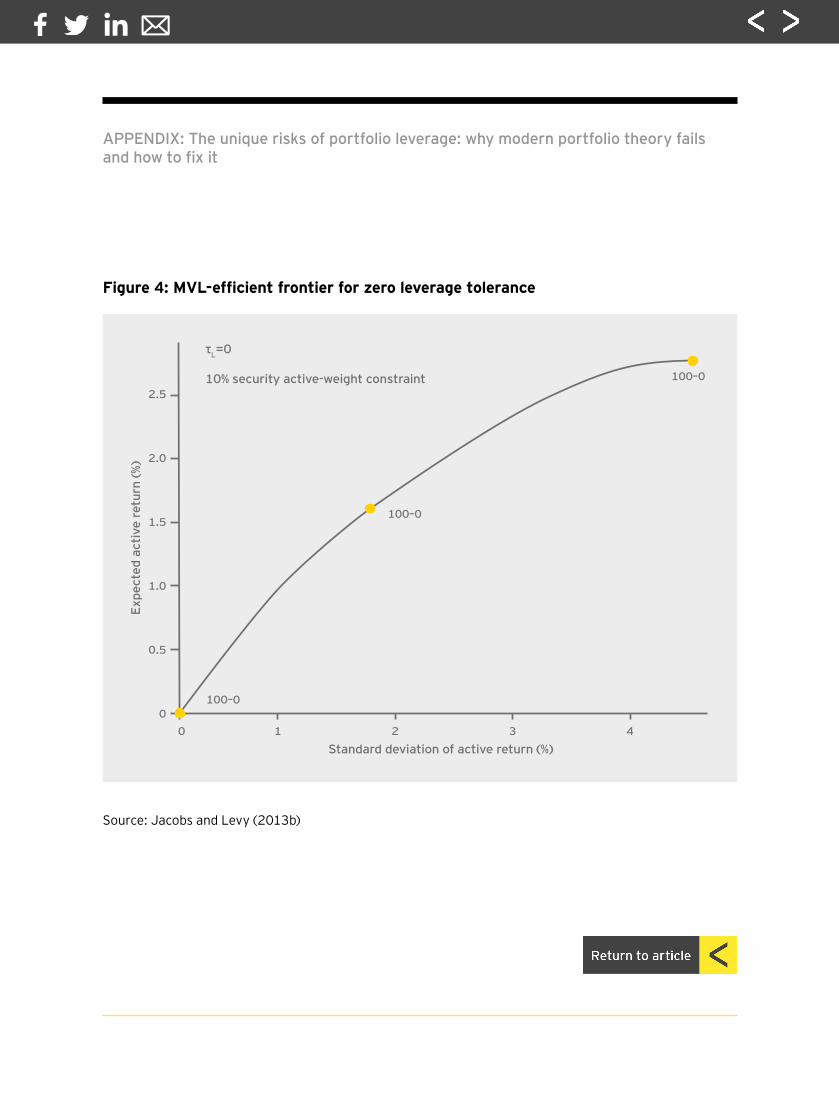
Figure 4 shows the efficient frontier based on MVL optimization for a range of investor volatility tolerances (0 to 2) when leverage tolerance is 0 ( = 0) and there is a 10%


12 Note that the expected active returns shown do not reflect any costs associated with leverage-related events, such as forced liquidation at adverse prices or bankruptcy. These costs, however, are reflected in the disutility implied by the leverage-aversion term.





constraint on security active weights. When no leverage is tolerated, all the efficientportfolios are long-only portfolios. The efficient frontier begins at the origin, corresponding to the efficient portfolio when volatility tolerance is zero; this portfolio is an index fund withzero expected active return and zero standard deviation of active return. As the volatility increases, the frontier rises at a declining rate, and efficient portfolios take more concentrated positions in securities with higher expected returns. In all cases, however,the leverage level remains 0; every portfolio along the frontier is a 100-0 portfolio, meaning it is invested 100% long, with no short or leveraged long positions. The MVL-efficient frontier with zero leverage tolerance and the MV-efficient frontier with a zero- leverage constraint are identical.13

Figure 5 illustrates the efficient frontier based on MVL optimization over the same range of volatility-tolerance levels when leverage tolerance is 1 ( = 1). Again, individual security positions are subject to the 10% active-weight constraint. Here, increasing volatility is accompanied by increasing leverage. The portfolios on the frontier go from 0 leverage to enhanced active portfolios of 110-10 to 130-30. From a comparison with Figure 4 (0 leverage tolerance), it can be seen that leverage allows a higher return at any given volatility level. Higher return and volatility risk can be achieved with less concentration of positions when leverage is allowed than when leverage is not allowed. For an investor with leverage tolerance of 1, any of the portfolios on the Figure 5 frontier can be optimal, depending on the investor’s level of volatility tolerance.

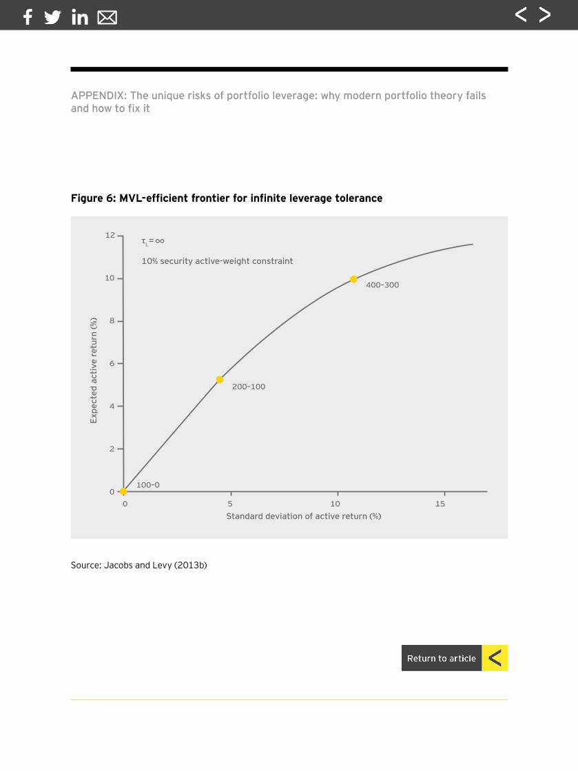
Figure 6 illustrates the efficient frontier across a range of volatility tolerances when leverage tolerance is infinite ( ). As the investor’s volatility tolerance increases, the portfolios on the frontier go from 0 leverage to enhanced active portfolios of 200-100 to 400-300. Relative to the investor with leverage tolerance of 1 (Figure 5), the investor with infinite leverage tolerance can achieve a higher expected return at any given levelof volatility, albeit with increasing leverage risk. As discussed earlier, conventional MV


13 The MVL utility function (Equation 2) reduces to the MV utility function (Equation 1) as the investor’s leverage tolerance, τL, approaches zero.





optimization implicitly assumes investors have infinite tolerance for the unique risks of leverage; thus the MV-efficient frontier is identical to the MVL-efficient frontier whenMVL optimization is based on infinite leverage tolerance.14

Figure 7 illustrates the efficient frontier based on MVL optimization when investor leverage tolerance is infinite ( ) and when there are no constraints on individual security activeweights. Again, leverage increases as volatility tolerance increases. Because each portfolio holds the same set of active positions at increasing levels of leverage, the efficient frontieris simply a straight line. Ever-higher levels of leverage are used to achieve ever-higher expected return along with ever-higher standard deviation of return. As with Figure 6, MVL optimization results in the same frontier as MV optimization, since the investor is assumed to have infinite leverage tolerance. The assumption of infinite leverage tolerance inherent in MV optimization can give rise to portfolios with unrealistically high levels of leverage.

Figure 8 displays efficient frontiers based on MVL optimization for a range of investor volatility tolerances (0 to 2) and leverage-tolerance levels corresponding to 0 (the same as in Figure 4), 0.5, 1.0 (the same as Figure 5), 1.5 and 2.0. Each frontier corresponds to one of these leverage-tolerance levels. Again, zero leverage tolerance represents an investor unwilling to use leverage, and higher efficient frontiers correspond to investorswith greater tolerances for leverage. The 10% security active-weight constraint applies to all the portfolios.

It might at first appear that the highest level of leverage tolerance results in the dominant efficient frontier; that is, higher leverage allows the investor to achieve higher expected returns at any given level of volatility. But when leverage aversion is considered,the optimal portfolio may lie on other frontiers, depending on the investor’s level of leverage tolerance.

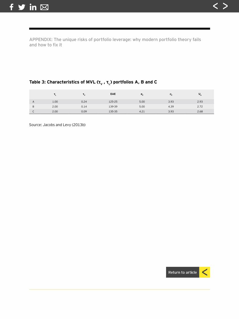
Consider, for example, the three portfolios represented by the points labeled A, B and C in Figure 8. These portfolios’ characteristics are provided in Table 3. Portfolio A is optimal for


14 The MVL utility function (Equation 2) reduces to the MV utility function (Equation 1) as the investor’s leverage tolerance, τL, increases without limit.





Investor A, who has a leverage tolerance ( ) of 1 and a volatility tolerance ( ) of 0.24. This is a 125-25 portfolio with a standard deviation of active return (σP) of 5% and an expected active return ( ) of 3.93%.

The last column of Table 3 shows that Investor A’s utility (UA) of Portfolio A is 2.93. In other words, Investor A is indifferent between Portfolio A, which has an expected active return of 3.93% along with volatility risk and leverage risk, and a hypothetical portfolio with a certain active return of 2.93% and no volatility or leverage risk. Put another way, it takes one full percentage point of additional return to get Investor A to accept the added volatility and leverage risk of Portfolio A in lieu of the hypothetical riskless portfolio.

Portfolio B offers a higher expected active return than Portfolio A (4.39% versus 3.93%) at the same volatility-risk level. But it is only optimal for an investor with a leverage tolerance of 2 and volatility tolerance of 0.14; it is suboptimal for Investor A, who has a lower leverage tolerance of 1. Portfolio B represents a 139-39 enhanced active portfolio; it entails significantly more leverage than the 125-25 Portfolio A.

For Investor A, the utility of Portfolio B is 2.72, lower than the 2.93 utility of Portfolio A. This investor’s desire to avoid additional leverage risk more than offsets the benefit of theincremental expected return.

Finally, consider Portfolio C, which has the same 3.93% expected active return as Portfolio A. This is the optimal portfolio for an investor who has a leverage tolerance of 2 and a volatility tolerance of 0.09. In a traditional MV framework, this portfolio dominates Portfolio A because it offers the same expected return at a lower standard deviation of active return. But it is nevertheless suboptimal for Investor A, who has a leverage tolerance of 1, for the same reason that Portfolio B is suboptimal: it entails more leverage than Portfolio A, 135-35 versus 125-25. Again, for Investor A, the lower expected volatility of Portfolio C is not enough to compensate for the increase in leverage risk. Investor A receives utility of 2.68 from Portfolio C, lower than the 2.93 from Portfolio A.






The mean-variance-leverage-efficient region The traditional MV-efficient frontier depicts the two-dimensional trade-off between mean and variance. MVL optimization adds a third dimension, leverage, allowing for trade-offs between mean, variance and leverage. Figure 9 depicts an efficient region of these trade-offs for investors with volatility tolerances between 0 and 2 and leverage tolerances between 0 and 2. There are no constraints on security weights. Which portfolio is optimal for a given investor depends on the investor’s tolerances for volatility risk and leverage risk. Figure 9 illustrates two-dimensional MV-efficient frontiers for several leverage-tolerance levels (the grey curved lines) and two-dimensional MV-efficient frontiers for several volatility-tolerance levels (the colored curved lines).15 The MVL optimal portfoliofor a leverage-averse investor is at the intersection of the efficient frontier for the investor’s volatility-tolerance level and the efficient frontier for the investor’s leverage-tolerance level. For example, the MVL(1,1) optimal portfolio is found where the efficient frontier for a leverage tolerance of 1 ( = 1) intersects with the black-colored frontier representing a volatility tolerance of 1 ( = 1).

The mean-variance-leverage-efficient surfaceA three-dimensional depiction of the MVL-efficient surface is presented in Figure 10. This surface was generated from 10,000 MVL optimizations using 100×100 pairs of volatility and leverage tolerances covering a range of values from 0.001 to 2 [Jacobs and Levy (2014)]. Note that the figure has three axes, one for volatility tolerance, one for leverage tolerance and one for level of enhancement (one-half of leverage). The optimal level ofenhancement emerges from an MVL optimization that considers both volatility tolerance and leverage tolerance.16


15 Because Figure 9 assumes no constraint on security active weights, each curve linking the optimal portfolios for an investor with a particular leverage tolerance level is smooth (unlike in Figure 8). Furthermore, without security active-weight constraints, both the standard deviation of active return and the expected active return for each efficient frontier range higher than in Figure 8.

16 To estimate their tolerances for volatility and leverage, investors could select different portfolios from the efficient surface, and for each portfolio run a Monte Carlo simulation that generates a probability distribution of ending wealth. Investors could then infer their volatility and leverage tolerances based on their preferred ending wealth distribution. Alternatively, investors could use asynchronous simulation, which can account for the occurrences of margin calls, including security liquidations at adverse prices [Jacobs et al. (2004, 2010)].





When leverage tolerance is zero, the optimal portfolios lie along the volatility-tolerance axis, having no leverage and hence no enhancement. They are long-only portfolios, taking active positions in accordance with the investor’s level of volatility tolerance. In this case, the same portfolios would be generated by either MV optimization or MVL optimization. As the investor’s leverage tolerance increases, however, the optimal level of enhancement increases at a slowly declining rate of increase.

When volatility tolerance is zero, the portfolios lie along the leverage-tolerance axis, having no active return volatility and hence holding benchmark weights in each security (an index fund). Again, either MV optimization or MVL optimization will produce the same portfolio. As investor volatility tolerance increases, however, the optimal level of enhancement picks up rapidly.

Another way to look at the relationships between optimal enhancement and volatility and leverage tolerances is to take horizontal cuts through the MVL-efficient surface. Figure 11provides a contour map of such cuts, with the color of each line corresponding to the same-colored enhancement on the MVL-efficient surface in Figure 10. Each line shows the combinations of volatility tolerance and leverage tolerance for which a given level of enhancement is optimal. For example, the 20% line shows the various combinations of volatility and leverage tolerances that lead to a 20% optimal enhancement. Optimal enhancement increases with leverage tolerance, but is approximately independent of volatility tolerance, if the latter is large enough.

The two solid black lines drawn over the efficient surface in Figure 10 and the contour map in Figure 11 correspond to optimal portfolios for investors having a volatility toleranceof 1 (and a range of values of leverage tolerance) and those for investors having a leverage tolerance of 1 (and a range of values of volatility tolerance). The MVL(1,1) optimal portfoliowould lie at the intersection of these two lines. In both figures, this portfolio is labeled “G.” The enhancement for this optimal portfolio is 29%, resulting in a 129-29 EAE portfolio. This portfolio provides the MVL(1,1) investor the highest utility of all the portfolios on the efficient surface.






Portfolio “G,” the optimal MVL(1,1) portfolio, has the same enhancement level as portfolio “g” in Figure 3. It also has the same standard deviation of active return and expectedactive return. In fact, portfolios “G” and “g” are identical: that is, they have the same holdings, and hence the same active weights. Portfolio “g,” however, was determined by considering numerous leverage-constrained MV(1) optimal portfolios and selecting the one that has the highest utility for an MVL(1,1) investor, according to an MVL utility function. In contrast, portfolio “G” was determined directly from an MVL(1,1) optimization, without the need for a leverage constraint.

The solid black line representing MVL optimal portfolios on the efficient surface or contour map at a volatility tolerance of 1 can be extended for levels of leverage tolerance beyond 2. Consider an MVL(1,∞) investor — that is, an investor with infinite leverage tolerance, or no leverage aversion. This investor is identical to an MV(1) investor with no leverage constraint. Now consider subjecting this investor to a leverage constraint, such thatenhancement is required to equal 29%. With this constraint, portfolio “G” is the optimal portfolio for an MV(1) investor, as it is for a leverage-unconstrained MVL(1,1) investor.

Alternatively, consider the yellow 29% contour line in Figure 11 (or the dashed line in Figure 10).17 This contour represents all portfolios on the efficient surface that have an enhancement of 29%. When the enhancement is constrained to equal 29%, the optimal portfolio must be somewhere on the 29% contour. Optimal portfolios for investors with a volatility tolerance of 1 (whatever their leverage tolerance) lie on the solid black verticalline representing a volatility tolerance of 1. Thus, portfolio “G” (the point at which the 29% contour intersects the solid vertical line representing a volatility tolerance of 1) is optimalfor an MV(1) investor who constrains the enhancement at 29%. Portfolios that are on the 29% contour, but not on the solid vertical line (representing a volatility tolerance of 1) would have lower utility than portfolio “G,” because the implied volatility tolerance of those portfolios would either be less than or greater than 1, departing from the investor’s volatility tolerance.


17 To the right of portfolio “G” in Figure 10, the dashed line is slightly below the solid line, but is visually indistinguishable from it.





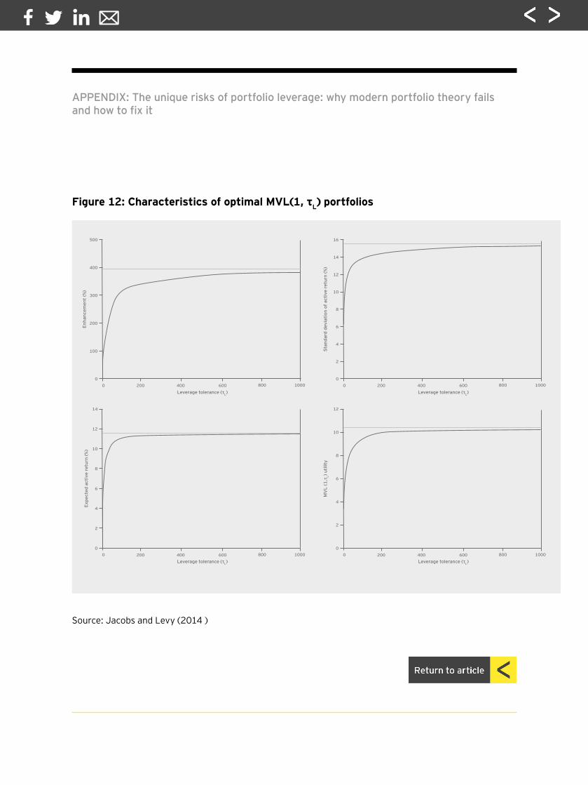
Optimal mean-variance-leverage portfolios versus optimal mean-variance portfoliosAs we have discussed, as leverage tolerance approaches infinity, the optimal MVL portfolios approach those determined by a conventional MV utility function. Figure 12 shows characteristics of optimal MVL(1, ) portfolios, with security active-weight constraints, as investor leverage tolerance, , increases from near 0 to 1,000. The characteristics displayed are enhancement, standard deviation of active return, expected active return and MVL(1, ) utility. The horizontal lines represent the levelsassociated with the optimal MV(1) portfolio “z” shown in Table 1.

All the characteristics initially rise rapidly and continue to increase, at a declining rate, as they converge to those of portfolio “z” as leverage tolerance approaches infinity.Except in the case of extreme leverage tolerance, the characteristics of the optimal MVL(1, ) portfolios are quite different from those of the optimal MV(1) portfolio, which are represented by the horizontal lines. Figure 12 shows that only by assuming an unreasonably large value for leverage tolerance would the solution to the MVL(1, ) problem be close to that of the MV(1) portfolio.

Volatility and leverage in real-life situationsThe optimal level of leverage in a portfolio is more than a theoretical concern. Figure 13 illustrates examples of various real-life combinations of volatility and leverage, ranging from the safe to the perilous. The top left of the figure, with low volatility and low leverage, is a long-only index fund. It represents the “safe” extreme, having no leverage and no active-return volatility.

At the bottom left, illustrating low volatility and high leverage, is the strategy pursued by Long-Term Capital Management (LTCM), the hedge fund that imploded in 1998. Its underlying holdings were supposedly low-risk arbitrage positions; however, the strategies were highly leveraged using shorting, borrowing and derivatives.

High volatility, even at low leverage levels, illustrated at top right, can also be perilous, as employees of Enron, the failed energy company, discovered. Many of them invested their savings in the company’s stock. When Enron declared bankruptcy in 2001, those employees learned how risky a volatile, undiversified portfolio can be.






The high-volatility, high-leverage extreme, at bottom right, is illustrated by the strategy followed by the chief executive officer of Chesapeake Energy. He borrowed on margin to leverage his bet on the company’s stock. Falling prices forced him to sell his leveraged position at a loss of nearly U.S. $2 billion in 2008.

Presumably, most of us are not at the extremes of either volatility or leverage, although we may have some leverage (a home mortgage, for example) and some volatile securities. The key is to make the optimal trade-off between expected return, volatility risk and leverage risk.

ConclusionUsing the MV model, an investor can address volatility tolerance and optimize a portfolio to provide the maximum level of expected return for any given level of volatility risk. Or alternatively, an investor can optimize a portfolio to provide the minimum level of volatility risk for any desired level of expected return. In either case, tolerance for the unique risks of leverage is not addressed, and MV optimal portfolios can be highly leveraged.

But we know that investors are willing to sacrifice some expected return in order to reduce leverage risk, just as they sacrifice some expected return in order to reduce volatility risk. Investors seeking to control portfolio leverage often choose a desired level of leverage based on the volatility of the securities, then impose that level by incorporating a leverage constraint in an MV optimization. As we have seen, however, MV optimizationwith leverage constraints will lead to the optimal portfolio for a leverage-averse investor only by chance.

The MVL model explicitly considers investor leverage tolerance as well as investor volatility tolerance. It thus allows the investor to determine, for any combination of leverage tolerance and volatility tolerance, the optimal portfolio. MVL optimization showsthat an investor’s level of leverage tolerance can have a large effect on portfolio choice.

Incorporating leverage aversion into portfolio optimization will result in less-leveraged portfolios than those produced with conventional MV optimization. This will be beneficial for leverage-averse investors because their portfolios will better reflect their preferences. A lower level of leverage in the financial system may also reduce the systemic risk that has repeatedly roiled the global economy.






ReferencesJacobs, B., 1999, Capital ideas and market realities: option replication, investor behavior, and stock market crashes, Blackwell PublishingJacobs, B., 2009, “Tumbling tower of Babel: subprime securitization and the credit crisis,” Financial Analysts Journal 65(2), 17-30Jacobs, B., and K. Levy, 2005, “A tale of two hedge funds,” in Jacobs, B., and K. Levy (eds.), Market neutral strategies, John Wiley and SonsJacobs, B., and K. Levy, 2007, “20 myths about enhanced active 120-20 strategies,” Financial Analysts Journal 63(4), 19-26Jacobs, B., and K. Levy, 2012, “Leverage aversion and portfolio optimality,” Financial Analysts Journal 68(5), 89-94Jacobs, B., and K. Levy, 2013a, “Introducing leverage aversion into portfolio theory and practice,” The Journal of Portfolio Management 39(2), 1-2Jacobs, B., and K. Levy, 2013b, “Leverage aversion, efficient frontiers, and the efficient region,” The Journal of Portfolio Management 39(3), 54-64Jacobs, B., and K. Levy, 2013c, “A comparison of the mean-variance-leverage optimization model and the Markowitz general mean-variance portfolio selection model,” The Journal of Portfolio Management 40(1), 1-5Jacobs, B., and K. Levy, 2014, “Traditional optimization is not optimal for leverage-averse investors,” The Journal of Portfolio Management 40(2), 1-11Jacobs, B., K. Levy, and H. Markowitz, 2004, “Financial market simulation,” The Journal of Portfolio Management 30(5), 142-151Jacobs, B., K. Levy, and H. Markowitz, 2010, “Simulating security markets in dynamic and equilibrium modes,” Financial Analysts Journal 66(5), 42-53Khandani, A., and A. Lo, 2007, “What happened to the quants in August 2007?” Journal of Investment Management 5(4), 29-78Kroll, Y., H. Levy, and H. Markowitz, 1984, “Mean-variance versus direct utility maximization,” The Journal of Finance 39(1), 47-61Levy, H., and H. Markowitz, 1979, “Approximating expected utility by a function of mean and variance,” The American Economic Review 69(3), 308-317Liu, S., and R. Xu, 2010, “Long-short optimization in Barra optimizer,” MSCI Barra Optimization ResearchMarkowitz, H., 1952, “Portfolio selection,” The Journal of Finance 7(1), 77-91Markowitz, H., 1959, Portfolio selection: efficient diversification of investments, Yale University Press; 2nd edition, Blackwell Publishing, 1991Markowitz, H., 2013, “How to represent mark-to-market possibilities with the general portfolio selection model,” The Journal of Portfolio Management 39(4), 1-3Melas, D., and R. Suryanarayanan, 2008, “130/30 implementation challenges,” MSCI Barra Research InsightsStefek, D., S. Liu, and R. Xu, 2012, “MSCI Barra optimizer,” MSCI Barra Portfolio Construction Research






AppendixThe unique risks of portfolio leverage: why modern portolio theory fails and how to fix it





Source: Jacobs and Levy (2014)

Figure 1: MV-efficient frontiers for various leverage constraints

APPENDIX: The unique risks of portfolio leverage: why modern portfolio theory fails and how to fix it

Expe

cted

act

ive

retu

rn (%

)

Standard deviation of active return (%)2

150–50 ( =1)

a

140–40 ( =0.8)

130–30 ( =0.6)

120–20 ( =0.4)

110–10 ( =0.2)

100–0 ( =0)

b

c

d

e

f

4 6 8

1

2

3

4

5





Figure 2: MV(1) utility of optimal MV(1) portfolios as a function of enhancement



10% security active-weight constraint

MV

(1) u

tilit

y

Enhancement (%)0 100 200 300 400 500

0

5

10

15

20

25

a b c d e f

Z

No security active-weight constraint






Table 1: Characteristics of optimal MV(1) portfolios from the perspective of an MV(1) investor

Portfolio EAE Leverage Standard deviation of active return

Expected active return Utility for an MV(1) investor

a 100-0 0 4.52 2.77 2.67

b 110-10 0.2 4.91 3.27 3.15

c 120-20 0.4 5.42 3.76 3.61

d 130-30 0.6 5.94 4.23 4.06

e 140-40 0.8 6.53 4.70 4.48

f 150-50 1.0 7.03 5.14 4.90

z 492-392 7.84 15.43 11.55 10.36







Table 2: Characteristics of optimal MV(1) portfolios from the perspective of an MVL(1,1) investor


Portfolio EAE Leverage Standard deviation of active return

Expected active return Utility for an MVL(1,1) investor

a 100-0 0 4.52 2.77 2.67

b 110-10 0.2 4.91 3.27 3.08

c 120-20 0.4 5.42 3.76 3.32

g 129-29 0.58 5.89 4.18 3.39

d 130-30 0.6 5.94 4.23 3.38

e 140-40 0.8 6.53 4.70 3.27

f 150-50 1.0 7.03 5.14 2.97






Figure 3: MVL(1,1) utility of optimal MV(1) portfolios as a function of enhancement


MV

L(1,

1) in

vest

or u

tilit

y

Enhancement (%)0 10 20 30 40 50

2.8

3.0

3.2

3.4

a

b

c

g

d

e

f





Source: Jacobs and Levy (2013b)

Figure 4: MVL-efficient frontier for zero leverage tolerance


Expe

cted

act

ive

retu

rn (%

)

Standard deviation of active return (%)0 1 2 3 4

0100–0

100–0

100–0

0.5

1.0

2.0

1.5

2.5

τL=0







Figure 5: MVL-efficient frontier for leverage tolerance of 1


Expe

cted

act

ive

retu

rn (%

)

Standard deviation of active return (%)0 1 2 3 4 5 6

0100–0

110–10

120–20

130–30

1

3

2

4

τL= 1







Figure 6: MVL-efficient frontier for infinite leverage tolerance


Expe

cted

act

ive

retu

rn (%

)

Standard deviation of active return (%)0 5

400–300

200–100

100–0

10 150

4

2

8

6

10

12τL=






Figure 7: MVL-efficient frontier for infinite leverage tolerance with no securityactive-weight constraint


Expe

cted

act

ive

retu

rn (%

)

Standard deviation of active return (%)0 50 100 150 200 250

0

100

50

200

150

250

300

100–0

4000–3900

9000–8900τL=

No security active-weight constraint






Figure 8: MVL-efficient frontiers for various leverage-tolerance cases with the 10% security active-weight constraint


Expe

cted

act

ive

retu

rn (%

)

Standard deviation of active return (%)0 42 6 8

A

B

C

0

2

1

4

3

5

τL= 2.0

τL= 1.5

τL= 1.0

τL= 0.5

τL= 0.0






Table 3: Characteristics of MVL (τV , τL) portfolios A, B and C


τL τV EAE σP αP UA

A 1.00 0.24 125-25 5.00 3.93 2.93

B 2.00 0.14 139-39 5.00 4.39 2.72

C 2.00 0.09 135-35 4.21 3.93 2.68






Figure 9: MVL-efficient region for various leverage and volatility-tolerance cases with no security active-weight constraint


Expe

cted

act

ive

retu

rn (%

)

Standard deviation of active return (%)0 42 6 12108

0

2

1

4

3

7

5

6

0.050.100.200.501.001.502.00

Volatility tolerance

τL=2.0

τL=1.5

τL=1.0

τL=0.5

τL=0.0






Figure 10: MVL-efficient surface


Volatility toleranceLeverage tolerance

Enha

ncem

ent

(%)

0 0

0.5

1

1.5

2

0.5

1

1.5

20

10

20

30

40

50

60

G






Figure 11: Contour map of the efficient surface


1.2

Leve

rage

tol

eran

ce

Volatility tolerance

G

5

10

15

20

25

29

35

40

45

50

0 0.60.40.2 10.8 1.8 21.61.40

0.6

0.4

0.2

1.2

1.4

0.8

1

2

1.6

1.8





Source: Jacobs and Levy (2014 )

Figure 12: Characteristics of optimal MVL(1, τL) portfolios


600400200 800 1000600400200 800 1000

600400200 800 1000

600400200 800 1000600400200 800 1000

Enha

ncem

ent

(%)

Leverage tolerance (τL)0

0

500

400

300

200

100 Stan

dard

dev

iati

on o

f act

ive

retu

rn (%

)


0

2

4

6

8

10

12

14

16

Expe

cted

act

ive

retu

rn (%

)


0

14

12

10

8

6

4

2

MV

L (1

,τL)

uti

lity


0

12

10

8

6

4

2





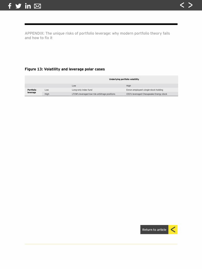
Figure 13: Volatility and leverage polar cases


Underlying portfolio volatility

Low High

Portfolio leverage

Low Long-only index fund Enron employee’s single-stock holding

High LTCM’s leveraged low-risk arbitrage positions CEO’s leveraged Chesapeake Energy stock





About EYEY is a global leader in assurance, tax, transaction and advisory services. The insights and quality services we deliver help build trust and confidence in the capital markets and in economies the world over. We develop outstanding leaders who team to deliver on our promises to all of our stakeholders. In so doing, we play a critical role in building a better working world for our people, for our clients and for our communities.

EY refers to the global organization, and may refer to one or more, of the member firms of Ernst & Young Global Limited, each of which is a separate legal entity. Ernst & Young Global Limited, a UK company limited by guarantee, does not provide services to clients. For more information about our organization, please visit ey.com.

© 2014 EYGM Limited. All Rights Reserved.EYG No. CQ0146

ey.com

The articles, information and reports (the articles) contained within The Journal are generic and represent the views and opinions of their authors. The articles produced by authors external to EY do not necessarily represent the views or opinions of EYGM Limited nor any other member of the global EY organization. The articles produced by EY contain general commentary and do not contain tailored specific advice and should not be regarded as comprehensive or sufficient for making decisions, nor should be used in place of professional advice. Accordingly, neither EYGM Limited nor any other member of the global EY organization accepts responsibility for loss arising from any action taken or not taken by those receiving The Journal.The views of third parties set out in this publication are not necessarily the views of the global EY organization or its member firms. Moreover, they should be seen in the context of the time they were made.

Accredited by the American Economic AssociationISSN 2049-8640





The Journal of Financial Perspectives - ey.com · portfolio construction method based on MPT, known...

Documents

Transcript of The Journal of Financial Perspectives - ey.com · portfolio construction method based on MPT, known...