1Lecture 12 Introduction to Prolog Logic Programming Prolog.
Computational Logic
The (ISO-)Prolog Programming Language
1

(ISO-)Prolog
• A practical programming language based on the logic programming paradigm.
• Main differences with “pure” logic programming:� depth-first search rule (also, left-to-right control rule),� more control of the execution flow,� many useful pre-defined predicates (some not declarative, for efficiency),� higher-order and meta-logical capabilities, ...
• Advantages:� it can be compiled into fast and efficient code (including native code),� more expressive power,� industry standard (ISO-Prolog),� mature implementations with modules, graphical environments, interfaces, ...
• Drawbacks of “classical” systems (and how addressed by modern systems):� Depth-first search rule is efficient but can lead to incompleteness→ alternative search strategies (e.g., Ciao’s bfall, tabling, etc.).� No occur check in unification (which led to unsoundness in older systems)→ support regular (i.e., infinite) trees: X = f(X) (already constraint-LP).
2
Programming Interface (Writing and Running Programs)
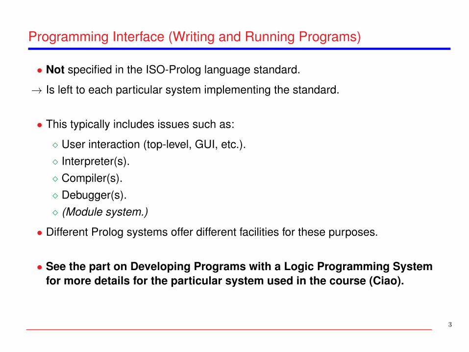
• Not specified in the ISO-Prolog language standard.
→ Is left to each particular system implementing the standard.
• This typically includes issues such as:
� User interaction (top-level, GUI, etc.).� Interpreter(s).� Compiler(s).� Debugger(s).� (Module system.)
• Different Prolog systems offer different facilities for these purposes.
• See the part on Developing Programs with a Logic Programming Systemfor more details for the particular system used in the course (Ciao).
3
Comparison with Imperative and Functional Languages
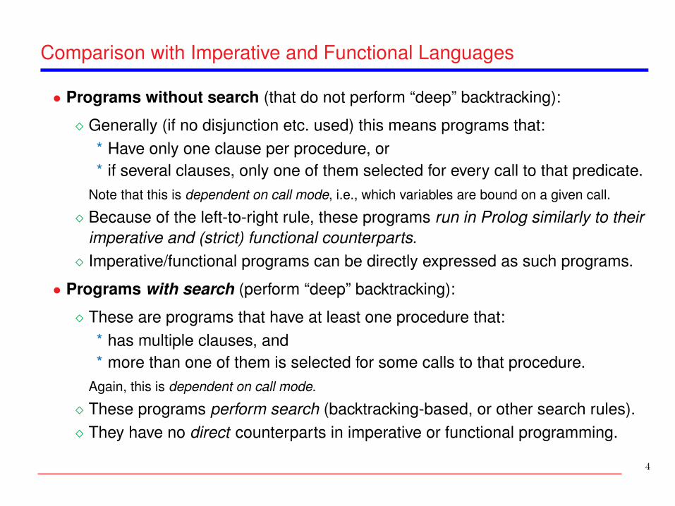
• Programs without search (that do not perform “deep” backtracking):
� Generally (if no disjunction etc. used) this means programs that:* Have only one clause per procedure, or* if several clauses, only one of them selected for every call to that predicate.
Note that this is dependent on call mode, i.e., which variables are bound on a given call.
� Because of the left-to-right rule, these programs run in Prolog similarly to theirimperative and (strict) functional counterparts.� Imperative/functional programs can be directly expressed as such programs.
• Programs with search (perform “deep” backtracking):
� These are programs that have at least one procedure that:* has multiple clauses, and* more than one of them is selected for some calls to that procedure.
Again, this is dependent on call mode.
� These programs perform search (backtracking-based, or other search rules).� They have no direct counterparts in imperative or functional programming.
4

Comparison with Imperative and Functional Languages (Contd.)
• Conventional languages and Prolog both implement (forward) continuations:the place to go after a procedure call succeeds. I.e., in:p(X,Y):- q(X,Z), r(Z,Y).
q(X,Z) :- ...
when the procedure call to q/2 finishes (with “success”), execution continues inp/2, just after the call to q/2, i.e., at the call to r/2 (the forward continuation).
• In Prolog, when there are procedures with multiple definitions, there is also abackward continuation: the place to go to if there is a failure. I.e., in:p(X,Y):- q(X,Z), r(Z,Y).
p(X,Y):- ...
q(X,Z) :- ...
if the call to q/2 succeeds, it is as above, but if it fails, execution continues at(“backtracks to”) the previous alternative: the second clause of p/2 (the backwardcontinuation).
• We say that p/2 has a choice point.
• Again, the debugger (see later) can be useful to observe how execution proceeds.5

Control of Search in Prolog
Again, conventional programs (no search) execute conventionally.
Programs with search: programmer has at least three ways of controlling execution:
1 The ordering of literals in the body of a clause:
• Profound effect on the size of the computation (in the limit, on termination).Compare executing p(X), q(X,Y) with executing q(X,Y), p(X) in:
p(X):- X = 4. q(X, Y):- X = 1, Y = a, ...
p(X):- X = 5. q(X, Y):- X = 2, Y = b, ...
q(X, Y):- X = 4, Y = c, ...
q(X, Y):- X = 4, Y = d, ...
p(X), q(X,Y) is more efficient: execution of p/2 reduces the choices of q/2.
• Note that optimal order depends on the variable instantiation mode:E.g., if in q(X,d), p(X) , this order is better than p(X), q(X,d) .
6

Control of Search in Prolog (Contd.)
2 The ordering of clauses in a predicate:
• Affects the order in which solutions are generated.E.g., in the previous example we get:X=4,Y=c as the first solution and X=4,Y=d as the second.If we reorder q/2:p(X):- X = 4. q(X, Y):- X = 4, Y = d, ...
p(X):- X = 5. q(X, Y):- X = 4, Y = c. ...
q(X, Y):- X = 2, Y = b, ...
q(X, Y):- X = 1, Y = a, ...
we get X=4,Y=d first and then X=4,Y=c .• If a subset of the solutions is requested, then clause order affects:� the size of the computation,� and, at the limit, termination!
Else, little significance unless computation is infinite and/or pruning is used.
3 The pruning operators (e.g., “cut”), which cut choices dynamically –see later.
7

The ISO Standard (Overview)
• Syntax (incl. operators) and operational semantics• Arithmetic• Checking basic types and state• Structure inspection and term comparison• Input/Output• Pruning operators (cut)• Meta-calls, higher-order, aggregation predicates• Negation as failure, cut-fail• Dynamic program modification• Meta-interpreters• Incomplete data structures• Exception handling
Additionally (not in standard):
• Definite Clause Grammars (DCGs): parsing
8

Prolog Syntax and Terminology
• Variables and constants as before:
� Variables (start with capital or ): X, Value, A, A1, 3, result.� Constants (start w/small letter or in ’ ’): x, =, [], ’Algol-3’, ’Don’’t’.
Note: in Prolog terminology constants are also referred to as “atoms.”
• Numbers: 0, 999, -77, 5.23, 0.23e-5, 0.23E-5.Infinite precision integers supported by many current systems (e.g., Ciao).
• Strings (of “codes”): "Prolog" = [80,114,111,108,111,103](list of ASCII character codes).
� Note: if ?- set_prolog_flag(write_strings, on).character lists are printed as strings: " " .
• Comments:
� Using % : rest of line is a comment.� Using /* ... */ : everything in between is a comment.
9

Prolog Syntax — Defining Operators
• Certain functors and predicate symbols are predefined as infix, prefix, or postfixoperators, aside from the standard term notation.
• Very useful to make programs (or data files) more readable.
• Stated using operator declarations::- op(< precedence >, < type >, < operator(s) >).
where:� < precedence >: is an integer from 1 to 1200.
E.g., if ‘+’ has higher precedence than ‘/’, thena+b/c ≡ a+(b/c) ≡ +(a,/(b,c)) .Otherwise, use parenthesis: /(+(a,b),c) ≡ (a+b)/c� < type >:
* infix: xfx (not associative), xfy (right associative), yfx (left associative).* prefix: fx (non-associative), fy (associative).* postfix: xf (non-associative), yf (associative).
� < operator(s) >: can be a single atom or a list of atoms.
10

Prolog Syntax — Operators (Contd.)
• Examples:Standard Notation Operator Notation’+’(a,’/’(b,c)) a+b/c
is(X, mod(34, 7)) X is 34 mod 7
’<’(’+’(3,4),8) 3+4 < 8
’=’(X,f(Y)) X = f(Y)
’-’(3) -3
spy(’/’(foo,3)) spy foo/3
’:-’(p(X),q(Y)) p(X) :- q(Y)
’:-’(p(X),’,’(q(Y),r(Z))) p(X) :- q(Y),r(Z)
• Note that, with this syntax convention, Prolog clauses are also Prolog terms!
• Parenthesis must always be used for operators with higher priority than 1000(i.e., the priority of ’,’): ..., assert( (p :-q)), ...
• Operators are local to modules (explained later).
11

Prolog Syntax — Operators (Contd.)
• Typical standard operators:
:- op( 1200, xfx, [ :-, --> ]).
:- op( 1200, fx, [ :-, ?- ]).
:- op( 1150, fx, [ mode, public, dynamic,
multifile , block, meta_predicate ,
parallel , sequential ]).
:- op( 1100, xfy, [ ; ]).
:- op( 1050, xfy, [ -> ]).
:- op( 1000, xfy, [ ’,’ ]).
:- op( 900, fy, [ \+, spy, nospy ]).
:- op( 700, xfx, [ =, is, =.., ==, \==, @<, @>, @=<, @>=,
=:=, =\=, <, >, =<, >= ]).
:- op( 550, xfy, [ : ]).
:- op( 500, yfx, [ +, -, #, /\, \/ ]).
:- op( 500, fx, [ +, - ]).
:- op( 400, yfx, [ *, /, //, <<, >> ]).
:- op( 300, xfx, [ mod ]).
:- op( 200, xfy, [ ˆ ]).
12

The Execution Mechanism of (classical) Prolog• Always execute calls in the body of clauses left-to-right.
• When entering a procedure, if several clauses unify (a choice point), take the firstunifying clause (i.e., the leftmost unexplored branch).
• On failure, backtrack to the next unexplored clause of the last choice point.
grandparent(C,G) :- parent(C,P), parent(P,G).
parent(C,P) :- father(C,P).
parent(C,P) :- mother(C,P).
father(charles,philip).
father(ana,george).
mother(charles,ana).
grandparent(charles,X)
parent(charles,P),parent(P,X)
mother(charles,P),parent(P,X)
parent(ana,X)
mother(ana,X)father(ana,X)mother(philip,X)father(philip,X)
parent(philip,X)
father(charles,P),parent(P,X)
failure failure failureX = george
• Check how Prolog explores this tree by running the debugger!
13

Built-in Arithmetic
• Practicality: interface to the underlying CPU arithmetic capabilities.
• These arithmetic operations are not as general as their logical counterparts.
• Interface: evaluator of arithmetic terms.
• The type of arithmetic terms (arithexpr/1 – in next slide):
� a number is an arithmetic term,� if f is an n-ary arithmetic functor and X1, ..., Xn are arithmetic terms thenf (X1, ..., Xn) is an arithmetic term.
• Arithmetic functors: +, -, *, / (float quotient), // (integer quotient), mod , ...(see later).
Examples:
� (3*X+Y)/Z , correct if when evaluated X, Y and Z are arithmetic terms,otherwise it will raise an error.� a+3*X raises an error (because a is not an arithmetic term).
14

Built-in Arithmetic (Contd.) – The arithexpr type
arithexpr :=
| num
| + arithexpr | - arithexpr
| ++ arithexpr | -- arithexpr
| aritexpr + arithexpr | aritexpr - arithexpr
| aritexpr * arithexpr | aritexpr // arithexpr
| aritexpr / arithexpr | abs(arithexpr)
| sign(arithexpr) | float_integer_part(arithexpr)
| float(arithexpr) | float_fractional_part(arithexpr)
| aritexpr ** arithexpr | exp(arithexpr)
| log(arithexpr) | sqrt(arithexpr)
| sin(arithexpr) | cos(arithexpr)
| atan(arithexpr) | [arithexpr]
|. . .
Other operators (see manuals):• rem, mod, gcd, >>, <<, /\, \/, \\, #, ...• integer, truncate, floor, round, ceiling, ...
15
Built-in Arithmetic (Contd.)
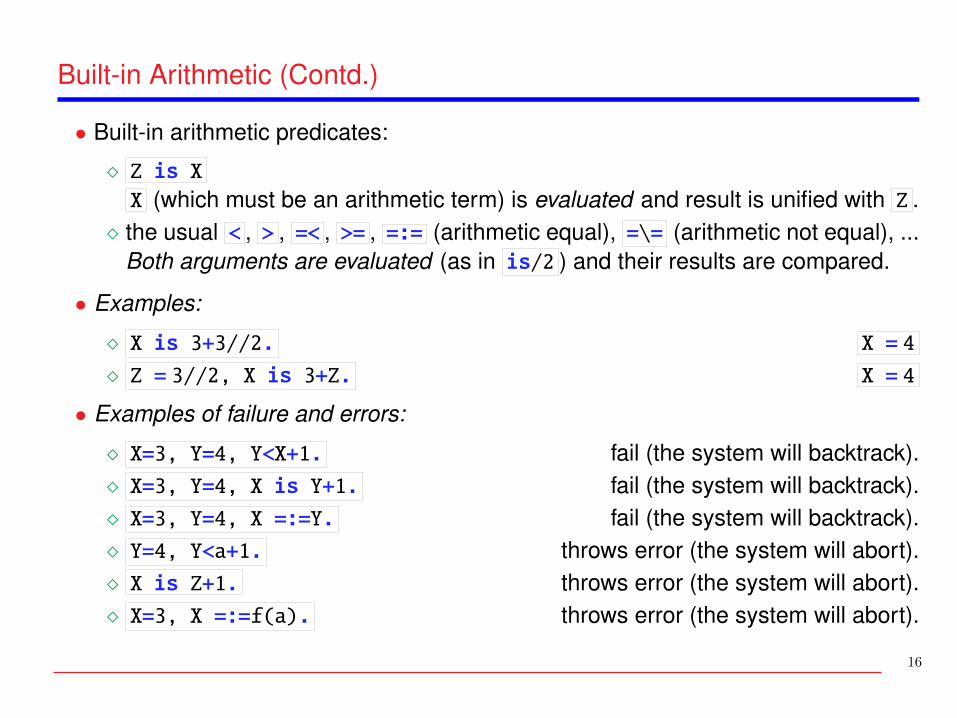
• Built-in arithmetic predicates:
� Z is XX (which must be an arithmetic term) is evaluated and result is unified with Z .
� the usual < , > , =< , >= , =:= (arithmetic equal), =\= (arithmetic not equal), ...Both arguments are evaluated (as in is/2 ) and their results are compared.
• Examples:
� X is 3+3//2. X = 4
� Z = 3//2, X is 3+Z. X = 4
• Examples of failure and errors:
� X=3, Y=4, Y<X+1. fail (the system will backtrack).� X=3, Y=4, X is Y+1. fail (the system will backtrack).� X=3, Y=4, X =:=Y. fail (the system will backtrack).� Y=4, Y<a+1. throws error (the system will abort).� X is Z+1. throws error (the system will abort).� X=3, X =:=f(a). throws error (the system will abort).
16
Arithmetic Programs
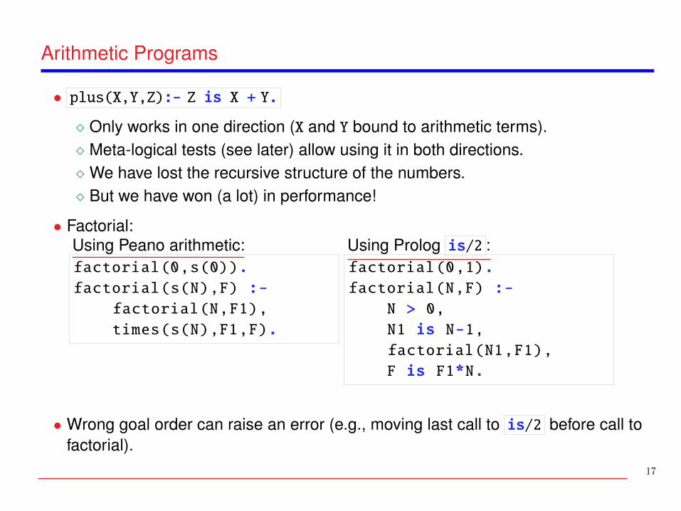
• plus(X,Y,Z):- Z is X + Y.
� Only works in one direction (X and Y bound to arithmetic terms).� Meta-logical tests (see later) allow using it in both directions.� We have lost the recursive structure of the numbers.� But we have won (a lot) in performance!
• Factorial:Using Peano arithmetic:factorial(0,s(0)).
factorial(s(N),F) :-
factorial(N,F1),
times(s(N),F1,F).
Using Prolog is/2 :factorial(0,1).
factorial(N,F) :-
N > 0,
N1 is N-1,
factorial(N1,F1),
F is F1*N.
• Wrong goal order can raise an error (e.g., moving last call to is/2 before call tofactorial).
17

Dynamic Checking of Basic Types
• Unary relations which check the type of a term:
� integer(X)� float(X)� number(X)� atom(X) (nonvariable term of arity 0 other than a number)� atomic(X) atom or number� ...
• They behave as if defined by a (possibly infinite) table of facts (in part, see below).
• They either succeed or fail, but do not produce an error.
• Thus, they cannot be used to generate (e.g., if argument is a variable, they failinstead of instantiating it to possible values).
• This behaviour is outside first order logic because it allows checking theinstantiation state of a variable.
18

Type Checking Predicates (Contd.)
• Example: implementing a better behavior for plus/3:plus(X,Y,Z) :- number(X), number(Y), Z is X + Y.
plus(X,Y,Z) :- number(X), number(Z), Y is Z - X.
plus(X,Y,Z) :- number(Y), number(Z), X is Z - Y.
Then:?- plus(3,Y,5).
Y = 2 ?
• Still, it cannot be used to partition a number into two others:?- plus(X,Y,5).
no
(in fact, this should raise an error, rather than simply failing).
19

Structure Inspection
• functor(X, F, A) :
� X is a term f(X1,...,Xn) → F=f A=n
� F is the atom f and A is the integer n → X = f(X1,..,Xn)
� Error if X, and either F or A are variables� Fails if the unification fails, A is not an integer, or F is not an atom
Examples:
� functor(t(b,a),F,A) → F=t, A=2 .� functor(Term,f,3) → Term =f(_,_,_) .� functor(Vector,v,100) → Vector =v(_, ... ,_) .
(Note: in some systems functor arity is limited to 256 by default;there are libraries that allow unbounded arrays.)
20

Structure Inspection (Contd.)
• arg(N, X, Arg) :
� N integer, X compound term→ Arg unified with N-th argument of X.� Allows accessing a structure argument in constant time and in a compact way.� Error if N is not an integer, or if X is a free variable.� Fails if the unification fails.
Examples:?- _T=date(9,February ,1947), arg(3,_T,X).
X = 1947
?- _T=date(9,February ,1947), _T=date(_,_,X).
X = 1947
?- functor(Array,array ,5),
arg(1,Array,black),
arg(5,Array,white).
Array = array(black,_,_,_,white).
• What does ?- arg(2,[a,b,c,d],X). return?
21

Example of Structure Inspection: Arrays
• Define add_arrays(A,B,C) :
add_arrays(A,B,C) :- % Same N below imposes equal length:
functor(A,array,N), functor(B,array,N), functor(C,array,N),
add_elements(N,A,B,C).
add_elements(0,_,_,_).
add_elements(I,A,B,C) :-
I>0, arg(I,A,AI), arg(I,B,BI), arg(I,C,CI),
CI is AI + BI, I1 is I - 1,
add_elements(I1,A,B,C).
• Alternative, using lists instead of structures:
add_arrays_lists([],[],[]).
add_arrays_lists([X|Xs],[Y|Ys],[Z|Zs]) :-
Z is X + Y,
add_arrays_lists(Xs,Ys,Zs).
• In the latter case, where do we check that the three lists are of equal length?
22

Example of Structure Inspection: Arrays (Contd.)
• Defining some syntactic sugar for arg/3 :
:- use_package(functional).
:- op(250,xfx,@). % Define @ as an infix operator
:- fun_eval ’@’/2. % Call @ when it appears as a term (no need for ˜)
@(T,N) := A :- arg(N,T,A). % Define @ as simply calling arg/3
• Now we can write add_elements/4 as:
add_elements(0,_,_,_).
add_elements(I,A,B,C) :-
I>0,
C@I is A@I + B@I,
add_elements(I-1,A,B,C).
23

Example of Structure Inspection: Subterms of a Term
• Define subterm(Sub,Term) :
subterm(Term,Term).
subterm(Sub,Term) :-
functor(Term,F,N),
subterm_args(N,Sub,Term).
subterm_args(N,Sub,Term) :-
arg(N,Term,Arg),% also checks N>0, arg fails otherwise!
subterm(Sub,Arg).
subterm_args(N,Sub,Term) :-
N>1,
N1 is N-1,
subterm_args(N1,Sub,Term).
24

Higher-Order Structure Inspection
• T =..L (read as “univ”)� L is the decomposition of a term T into a list comprising its principal functor
followed by its arguments.?- date(9,february ,1947) =.. L.
L = [date,9,february ,1947].
?- _F = ’+’, X =.. [_F,a,b].
X = a + b.
� Allows implementing higher-order primitives (see later).Example (extending derivative):deriv(sin(X),X,cos(X)).
deriv(cos(X),X,-sin(X)).
deriv(FG_X, X, DF_G * DG_X) :-
FG_X =.. [_, G_X],
deriv(FG_X, G_X, DF_G), deriv(G_X, X, DG_X).
?- deriv(sin(cos(x)),x,D).
D = cos(cos(x))* -sin(x) ?
� But use only when strictly necessary: expensive in time and memory, HO.
25

Conversion Between Strings and Atoms (New Atom Creation)
• Classical primitive: name(A,S)� A is the atom/number whose name is the list of ASCII characters S?- name(hello,S).
S = [104,101,108,108,111]
?- name(A,[104,101,108,108,111]).
A = hello
?- name(A,"hello").
A = hello
� Ambiguity when converting strings which represent numbers.Example: ?- name(’1’,X), name(Y,X).� In the ISO standard fixed by dividing into two:
* atom_codes(Atom,String)* number_codes(Number,String)
26

Meta-Logical Predicates
• var(X) : succeed iff X is a free variable.
?- var(X), X =f(a).%Succeeds
?- X = f(a), var(X).% Fails
• nonvar(X) : succeed iff X is not a free variable.
?- X = f(Y), nonvar(X).%Succeeds
• ground(X) : succeed iff X is fully instantiated.
?- X = f(Y), ground(X).%Fails
• Outside the scope of first order logic.
• Uses:
� control goal order,� restore some flexibility to programs using certain builtins.
27

Meta-Logical Predicates (Contd.) – choosing implementations
• Example: list length:length([],0).
length([_|T],N) :- length(T,TN), N is TN+1.
• Choosing between two implementations based on calling mode.I.e., implementing reversibility ”by hand.”length(L,N) :- var(L), integer(N), create_list(N,L).
length(L,N) :- nonvar(L), compute_length(L,N).
create_list(0,[]).
create_list(N,[_|T]) :- N > 0, NT is N-1, create_list(NT,T).
compute_length([],0).
compute_length([_|T],N) :- compute_length(T,TN), N is TN+1.
• Not really needed: the normal definition of length is actually reversible!
• Although reversing traditional list length is less efficient than length num(N,L)when L is a variable and N a number.
28
Meta-Logical Predicates (Contd.) – choosing implementations
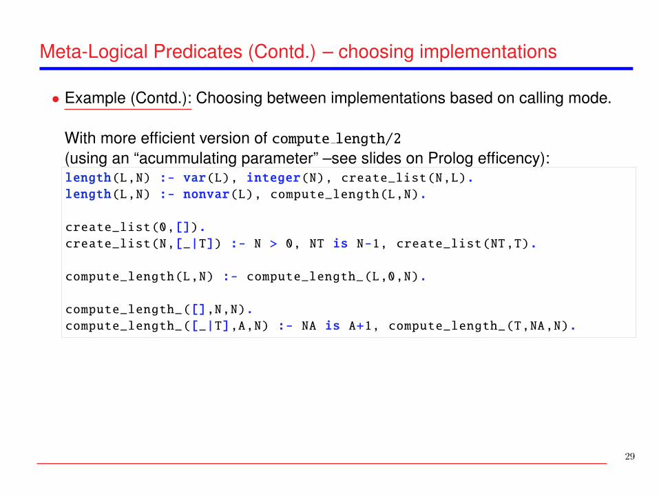
• Example (Contd.): Choosing between implementations based on calling mode.
With more efficient version of compute length/2(using an “acummulating parameter” –see slides on Prolog efficency):length(L,N) :- var(L), integer(N), create_list(N,L).
length(L,N) :- nonvar(L), compute_length(L,N).
create_list(0,[]).
create_list(N,[_|T]) :- N > 0, NT is N-1, create_list(NT,T).
compute_length(L,N) :- compute_length_(L,0,N).
compute_length_([],N,N).
compute_length_([_|T],A,N) :- NA is A+1, compute_length_(T,NA,N).
29
Comparing Non-ground Terms
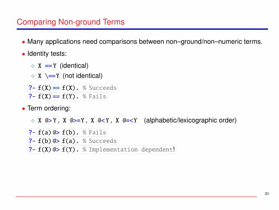
• Many applications need comparisons between non–ground/non–numeric terms.
• Identity tests:
� X ==Y (identical)� X \==Y (not identical)
?- f(X)== f(X). % Succeeds
?- f(X)== f(Y). % Fails
• Term ordering:
� X @>Y , X @>=Y , X @<Y , X @=<Y (alphabetic/lexicographic order)
?- f(a)@> f(b). % Fails
?- f(b)@> f(a). % Succeeds
?- f(X)@> f(Y). % Implementation dependent!
30

Comparing Non-ground Terms (Contd.)
• Reconsider subterm/2 with non-ground termssubterm(Sub,Term) :- Sub == Term.
subterm(Sub,Term) :- nonvar(Term),
functor(Term,F,N),
subterm(N,Sub,Term).
where subterm/3 is identical to the previous definition
• Insert an item into an ordered list:insert([], Item,[Item]).
insert([H|T],Item,[H|T]) :- H == Item.
insert([H|T],Item,[Item, H|T]) :- H @> Item.
insert([H|T],Item,[H|NewT]) :- H @< Item,
insert(T, Item, NewT).
• Compare with the same program with the second clause defined asinsert([H|T], Item, [Item|T]):- H = Item.
31

Input/Output
• A minimal set of input-output predicates (“DEC-10 Prolog I/O”):
Class Predicate ExplanationI/O stream control see(File) File becomes the current input stream.
seeing(File) The current input stream is File.seen Close the current input stream.tell(File) File becomes the current output stream.telling(File) The current output stream is File.told Close the current output stream.
Term I/O write(X) Write the term X on the current output stream.nl Start a new line on the current output stream.read(X) Read a term (finished by a full stop) from the
current input stream and unify it with X.Character I/O put_code(N) Write the ASCII character code N. N can be a
string of length one.get_code(N) Read the next character code and unify its
ASCII code with N.
32
Input/Output (Contd.)
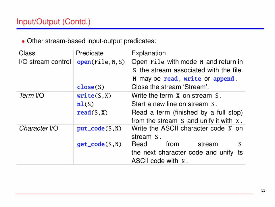
• Other stream-based input-output predicates:
Class Predicate ExplanationI/O stream control open(File,M,S) Open File with mode M and return in
S the stream associated with the file.M may be read , write or append .
close(S) Close the stream ‘Stream’.Term I/O write(S,X) Write the term X on stream S .
nl(S) Start a new line on stream S .read(S,X) Read a term (finished by a full stop)
from the stream S and unify it with X .Character I/O put_code(S,N) Write the ASCII character code N on
stream S .get_code(S,N) Read from stream S
the next character code and unify itsASCII code with N .
33
Input/Output (Contd.)
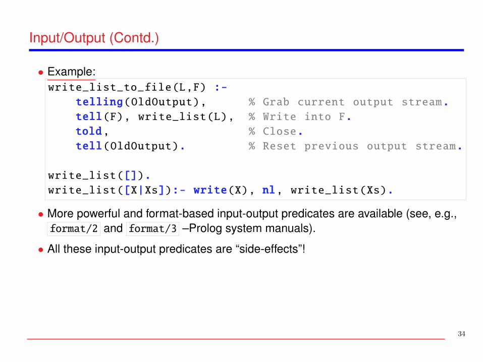
• Example:write_list_to_file(L,F) :-
telling(OldOutput), % Grab current output stream.
tell(F), write_list(L), % Write into F.
told, % Close.
tell(OldOutput). % Reset previous output stream.
write_list([]).
write_list([X|Xs]):- write(X), nl, write_list(Xs).
• More powerful and format-based input-output predicates are available (see, e.g.,format/2 and format/3 –Prolog system manuals).
• All these input-output predicates are “side-effects”!
34

Pruning Operator: Cut
• A “cut” (predicate !/0 ) commits Prolog to all the choices made since the parentgoal was unified with the head of the clause in which the cut appears.
• Thus, it prunes:
� all clauses below the clause in which the cut appears, and� all alternative solutions to the goals in the clause to the left of the cut.
But it does not affect the search in the goals to the right of the cut.s(1). p(X,Y):- l(X), ... r(8).
s(2). p(X,Y):- r(X), !, ... r(9).
p(X,Y):- m(X), ...
with query ?- s(A),p(B,C) .If execution reaches the cut ( ! ):
� The second alternative of r/1 is not considered.� The third clause of p/2 is not considered.
35

Pruning Operator: Cut (Contd.)
s(1). p(X,Y):- l(X), ... r(8).
s(2). p(X,Y):- r(X), !, ... r(9).
p(X,Y):- m(X), ...
!,...
| ?− s(A), p(B,C).A/1
p(B,C)
l(B), ... r(B),!,... m(B), ...
B/8 B/9
A/2
p(B,C)
l(B), ... r(B),!,... m(B), ...
B/9B/8
!,...
36
“Types” of Cut
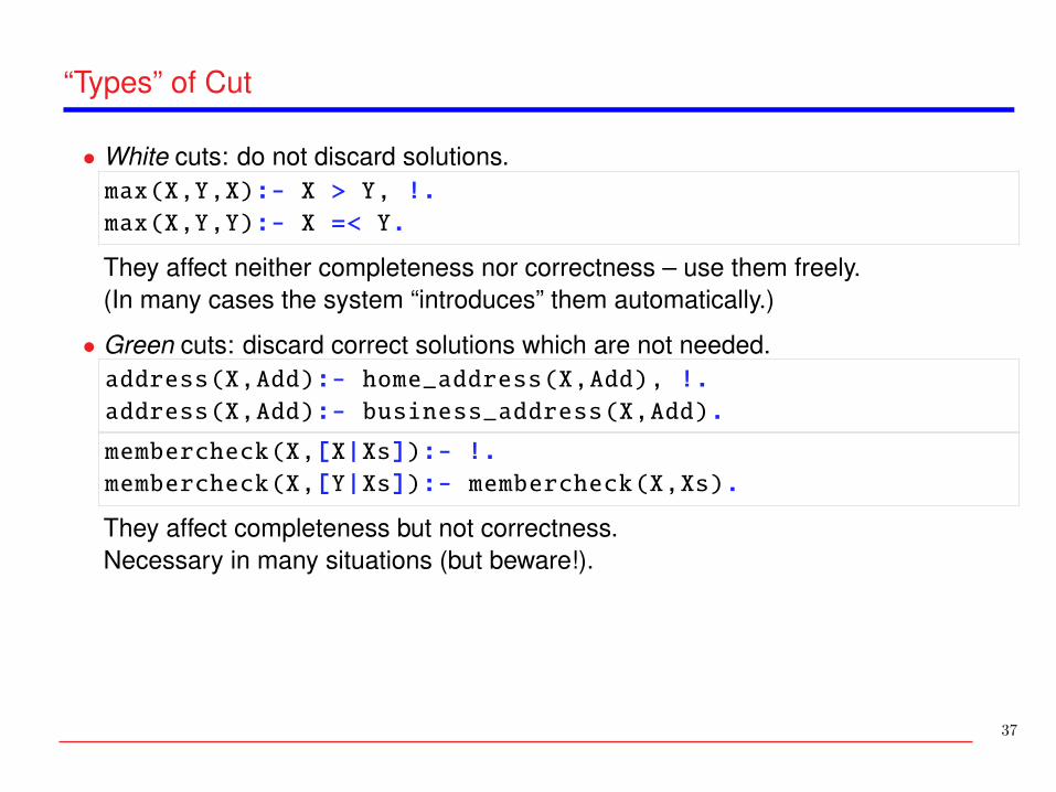
• White cuts: do not discard solutions.max(X,Y,X):- X > Y, !.
max(X,Y,Y):- X =< Y.
They affect neither completeness nor correctness – use them freely.(In many cases the system “introduces” them automatically.)
• Green cuts: discard correct solutions which are not needed.address(X,Add):- home_address(X,Add), !.
address(X,Add):- business_address(X,Add).
membercheck(X,[X|Xs]):- !.
membercheck(X,[Y|Xs]):- membercheck(X,Xs).
They affect completeness but not correctness.Necessary in many situations (but beware!).
37
“Types” of Cut (Contd.)
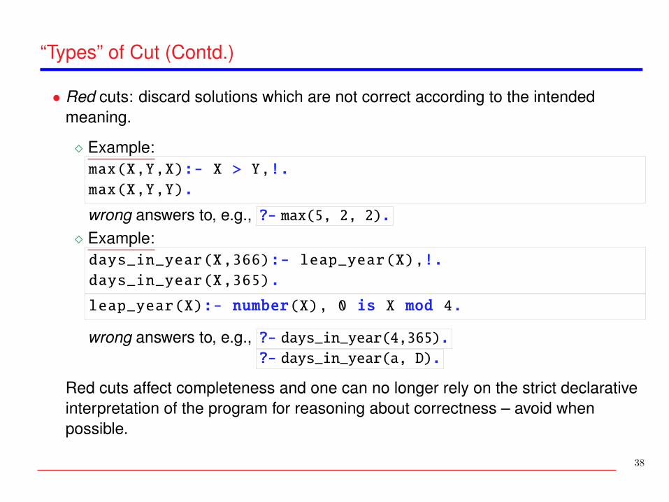
• Red cuts: discard solutions which are not correct according to the intendedmeaning.
� Example:max(X,Y,X):- X > Y,!.
max(X,Y,Y).
wrong answers to, e.g., ?- max(5, 2, 2).� Example:days_in_year(X,366):- leap_year(X),!.
days_in_year(X,365).
leap_year(X):- number(X), 0 is X mod 4.
wrong answers to, e.g., ?- days_in_year(4,365).?- days_in_year(a, D).
Red cuts affect completeness and one can no longer rely on the strict declarativeinterpretation of the program for reasoning about correctness – avoid whenpossible.
38
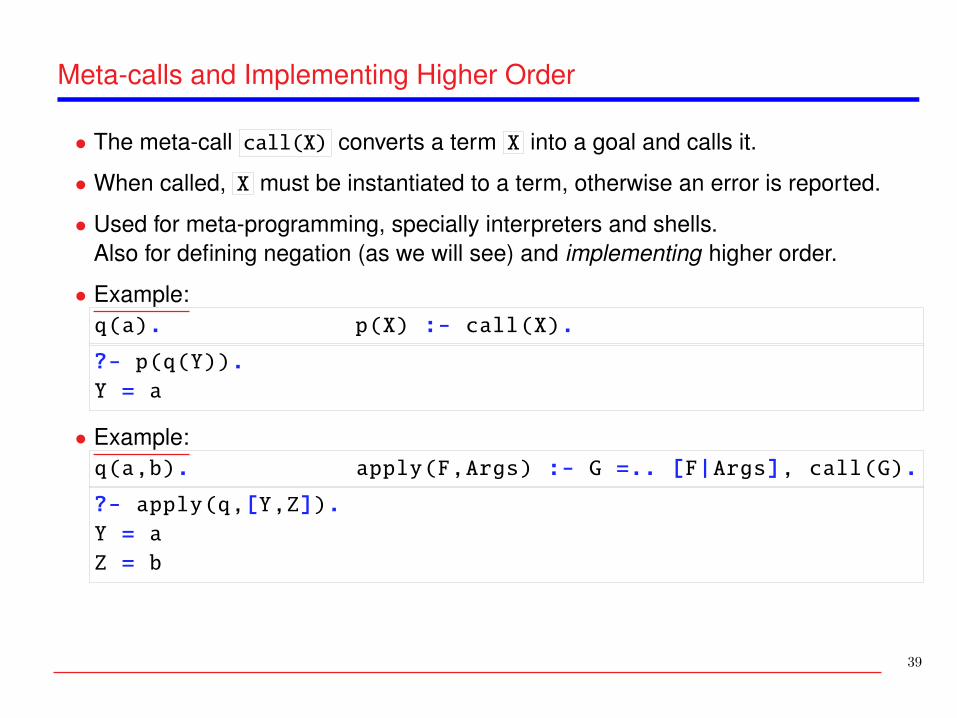
Meta-calls and Implementing Higher Order
• The meta-call call(X) converts a term X into a goal and calls it.
• When called, X must be instantiated to a term, otherwise an error is reported.
• Used for meta-programming, specially interpreters and shells.Also for defining negation (as we will see) and implementing higher order.
• Example:q(a). p(X) :- call(X).
?- p(q(Y)).
Y = a
• Example:q(a,b). apply(F,Args) :- G =.. [F|Args], call(G).
?- apply(q,[Y,Z]).
Y = a
Z = b
39
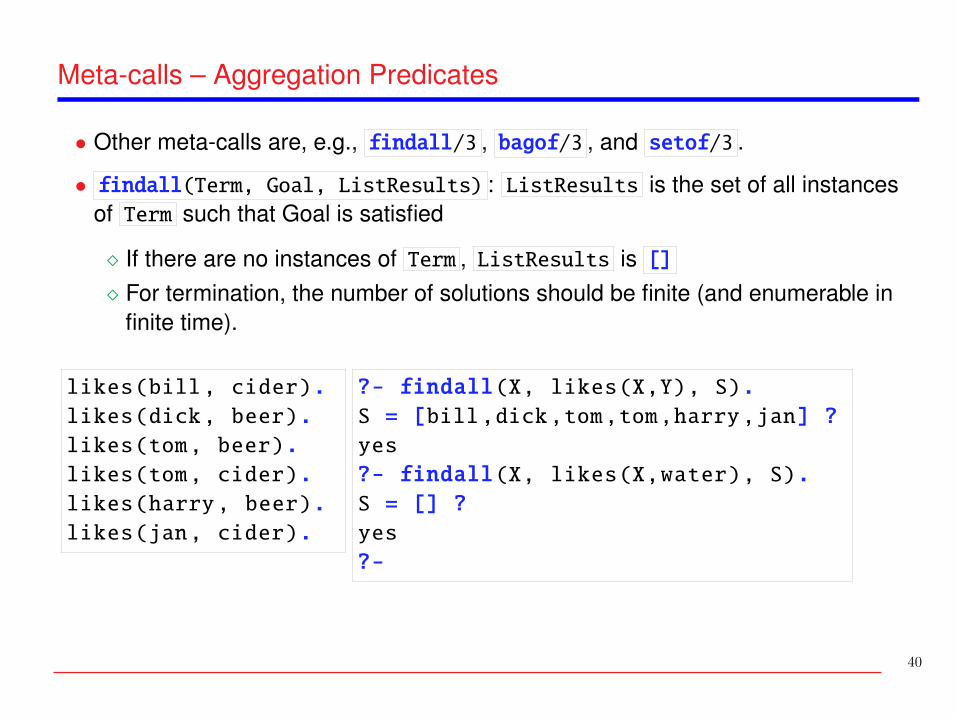
Meta-calls – Aggregation Predicates
• Other meta-calls are, e.g., findall/3 , bagof/3 , and setof/3 .
• findall(Term, Goal, ListResults) : ListResults is the set of all instancesof Term such that Goal is satisfied
� If there are no instances of Term , ListResults is []� For termination, the number of solutions should be finite (and enumerable in
finite time).
likes(bill, cider).
likes(dick, beer).
likes(tom, beer).
likes(tom, cider).
likes(harry, beer).
likes(jan, cider).
?- findall(X, likes(X,Y), S).
S = [bill,dick,tom,tom,harry,jan] ?
yes
?- findall(X, likes(X,water), S).
S = [] ?
yes
?-
40

Meta-calls – Aggregation Predicates (Contd.)
• setof(Term, Goal, ListResults) : ListResults is the ordered set (noduplicates) of all instances of Term such that Goal is satisfied
� If there are no instances of Term the predicate fails� The set should be finite (and enumerable in finite time)� If there are un-instantiated variables in Goal which do not also appear inTerm then a call to this built-in predicate may backtrack, generating alternativevalues for ListResults corresponding to different instantiations of the freevariables of Goal� Variables in Goal will not be treated as free if they are explicitly bound withinGoal by an existential quantifier as in Yˆ...(then, they behave as in findall/3 )
• bagof/3 :same, but returns list unsorted and with duplicates (in backtracking order).
41

Meta-calls – Aggregation Predicates: Examples
likes(bill, cider).
likes(dick, beer).
likes(harry, beer).
likes(jan, cider).
likes(tom, beer).
likes(tom, cider).
?- setof(X, likes(X,Y), S).
S = [dick,harry,tom],
Y = beer ? ;
S = [bill,jan,tom],
Y = cider ? ;
no
?- setof((Y,S), setof(X, likes(X,Y), S), SS).
SS = [(beer,[dick,harry,tom]),
(cider,[bill,jan,tom])] ? ;
no
?- setof(X, Yˆ(likes(X,Y)), S).
S = [bill,dick,harry,jan,tom] ? ;
no
42

Meta-calls – Negation as Failure
• Uses the meta-call facilities, the cut and a system predicate fail that fails whenexecuted (similar to calling a=b ).not(Goal) :- call(Goal), !, fail.
not(Goal).
• Available as the (prefix) predicate \+/1 : \+ member(c, [a,k,l])
• It will never instantiate variables.� Using \+ twice useful to test without binding variables. E.g., \+ \+ X = 1 ,
checks if X is bound (or can be bound) to 1, without binding X if is free.
• Termination of not(Goal) depends on termination of Goal . not(Goal) willterminate if a success node for Goal is found before an infinite branch.• It is very useful but dangerous:unmarried_student(X):- not(married(X)), student(X).
student(joe).
married(john).
?- unmarried_student(X). → no• Works correctly for ground goals (programmer’s responsibility to ensure this).
43

Meta-calls – Negation as Failure – Ensuring Correctness
• We can check that negation is called with a ground term:not(G) :-
ground(G), !,
\+ G.
not(G) :-
write(’ERROR: Non-ground goal in negation: ’), write(G), nl,
abort.
• Or using assertions::- pred not(G) : ground(G).
not(G) :- \+ G.
I.e., we declare that G must be ground when called ( : field).
This will be checked, e.g., dynamically if we turn on run-time checking::- use_package([rtchecks]).
44
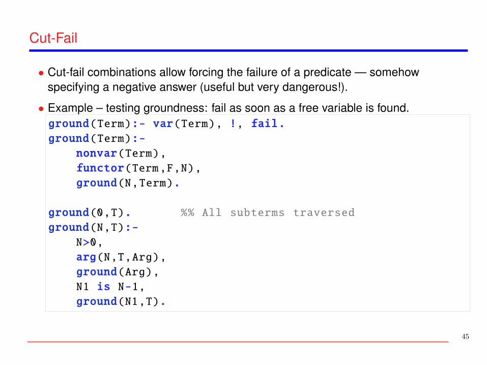
Cut-Fail
• Cut-fail combinations allow forcing the failure of a predicate — somehowspecifying a negative answer (useful but very dangerous!).
• Example – testing groundness: fail as soon as a free variable is found.ground(Term):- var(Term), !, fail.
ground(Term):-
nonvar(Term),
functor(Term,F,N),
ground(N,Term).
ground(0,T). %% All subterms traversed
ground(N,T):-
N>0,
arg(N,T,Arg),
ground(Arg),
N1 is N-1,
ground(N1,T).
45

Dynamic Program Modification (I)
• assert/1 , retract/1 , abolish/1 , ...
• Very powerful: allow run–time modification of programs. Can also be used tosimulate global variables.
• Sometimes this is very useful, but very often a mistake:
� Code hard to read, hard to understand, hard to debug.� Typically, slow.
• Program modification has to be used scarcely, carefully, locally.
• Still, assertion and retraction can be logically justified in some cases:
� Assertion of clauses which logically follow from the program. (lemmas)� Retraction of clauses which are logically redundant.
• Other typically non-harmful use: simple global switches.
• Behavior/requirements may differ between Prolog implementations.Typically, the predicate must be declared :- dynamic .
46

Dynamic Program Modification (II)
• Example program:relate_numbers(X, Y):- assert(related(X, Y)).
unrelate_numbers(X, Y):- retract(related(X, Y)).
• Example query:?- related(1, 2).
{EXISTENCE ERROR: ...}
?- relate_numbers(1, 2).
yes
?- related(1, 2).
yes
?- unrelate_numbers(1, 2).
yes
?- related(1, 2).
no
• Rules can be asserted dynamically as well.
47
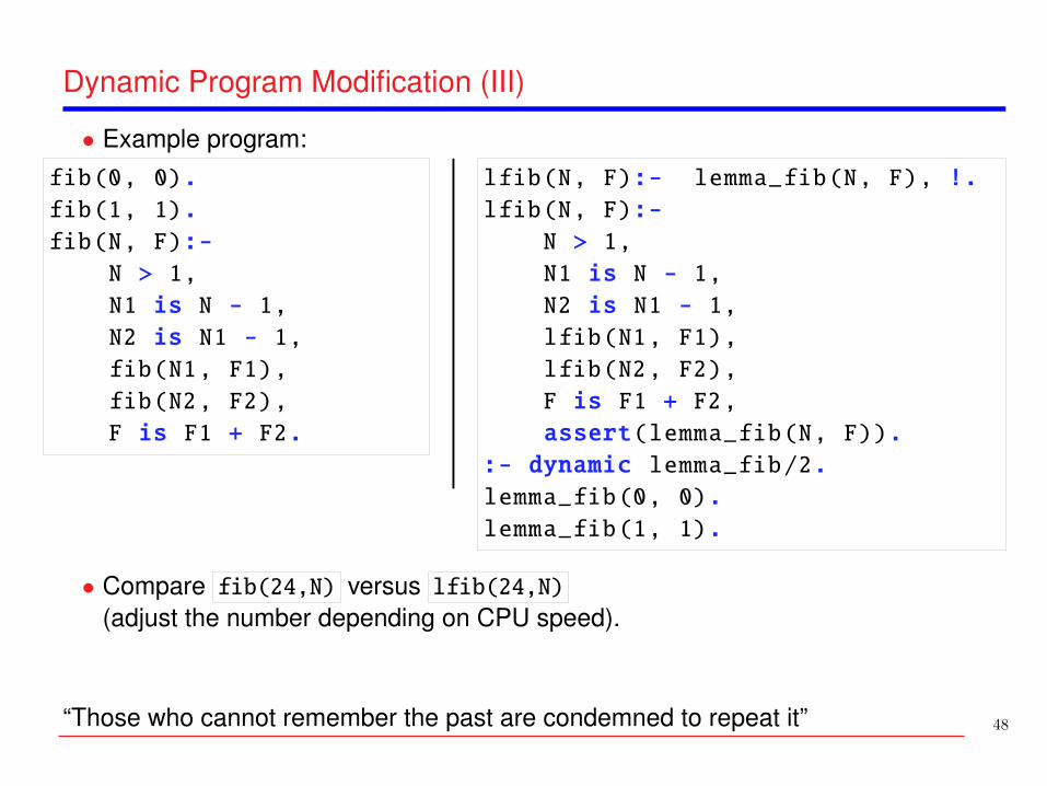
Dynamic Program Modification (III)
• Example program:fib(0, 0).
fib(1, 1).
fib(N, F):-
N > 1,
N1 is N - 1,
N2 is N1 - 1,
fib(N1, F1),
fib(N2, F2),
F is F1 + F2.
lfib(N, F):- lemma_fib(N, F), !.
lfib(N, F):-
N > 1,
N1 is N - 1,
N2 is N1 - 1,
lfib(N1, F1),
lfib(N2, F2),
F is F1 + F2,
assert(lemma_fib(N, F)).
:- dynamic lemma_fib/2.
lemma_fib(0, 0).
lemma_fib(1, 1).
• Compare fib(24,N) versus lfib(24,N)(adjust the number depending on CPU speed).
“Those who cannot remember the past are condemned to repeat it” 48
Meta-Interpreters
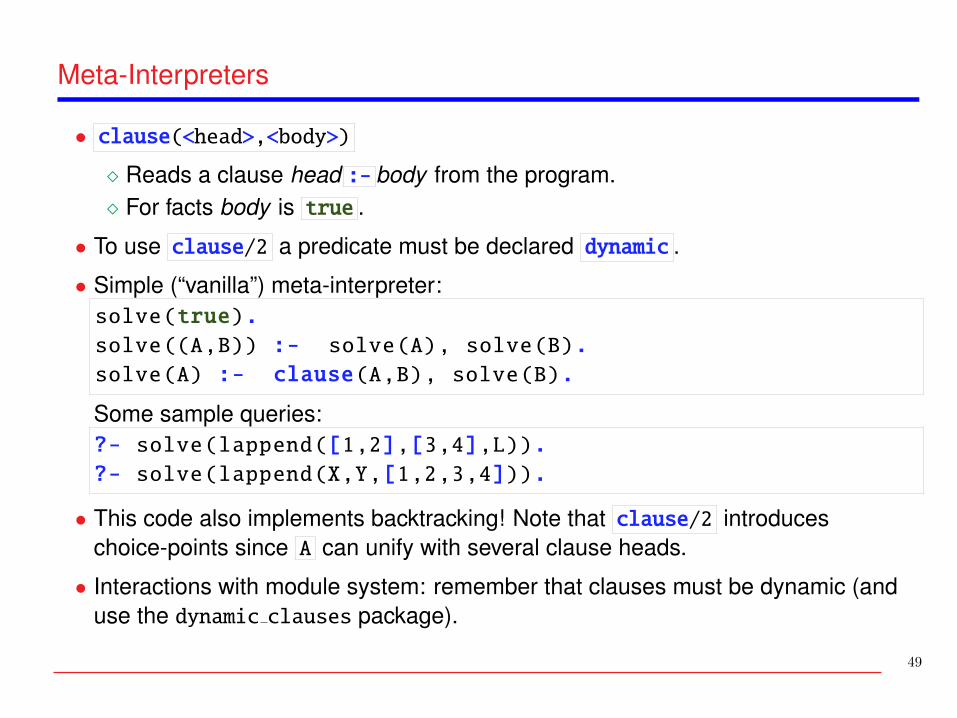
• clause(<head>,<body>)� Reads a clause head :- body from the program.� For facts body is true .
• To use clause/2 a predicate must be declared dynamic .
• Simple (“vanilla”) meta-interpreter:solve(true).
solve((A,B)) :- solve(A), solve(B).
solve(A) :- clause(A,B), solve(B).
Some sample queries:?- solve(lappend([1,2],[3,4],L)).
?- solve(lappend(X,Y,[1,2,3,4])).
• This code also implements backtracking! Note that clause/2 introduceschoice-points since A can unify with several clause heads.
• Interactions with module system: remember that clauses must be dynamic (anduse the dynamic clauses package).
49

Meta-Interpreters: extending the basic meta-interpreter
• The basic meta-interpreter code:solve(true).
solve((A,B)) :- solve(A), solve(B).
solve(A) :- clause(A,B), solve(B).
can be easily extended to do many tasks: tracing, debugging, explanations inexpert systems, implementing other computation rules, ...
• E.g., an interpreter that counts the number of (forward) steps:csolve( true, 0).
csolve( (A,B), N) :- csolve(A,NA), csolve(B,NB), N is NA+NB.
csolve( A, N) :- clause(A,B), csolve(B,N1), N is N1+1.
?- csolve(lappend([1,2],[3,4],L),N).
50

Incomplete Data Structures
• Example – difference lists:
� A pseudo-type:dlist(X-Y) :- var(X), !, X==Y.
dlist([_|DL]-Y) :- dlist(DL-Y).
(Note: just for “minimal” difference lists, and not declarative because of ==/2 )
� Allows us to keep a pointer to the end of the list.
� Allows appending in constant time:append_dl(B1-E1,B2-E2,B3-E3) :- B3=B1, E3=E2, B2=E1.
Or, more compactly:append_dl(X-Y,Y-Z,X-Z).
And, actually, no call to append_dl is normally necessary!
... But can only be done once (see later).
• Also one can build difference (open ended) trees, dictionaries, queues, etc., byleaving variables at the ends (e.g., at the leaves for trees).
51
Playing with difference lists
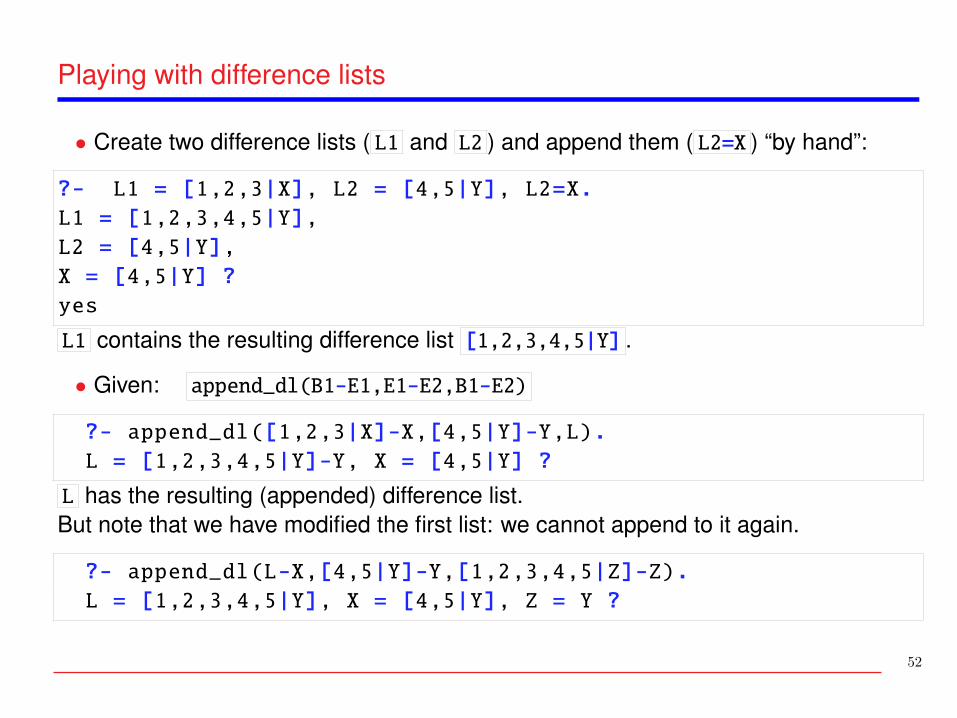
• Create two difference lists ( L1 and L2 ) and append them ( L2=X ) “by hand”:
?- L1 = [1,2,3|X], L2 = [4,5|Y], L2=X.
L1 = [1,2,3,4,5|Y],
L2 = [4,5|Y],
X = [4,5|Y] ?
yes
L1 contains the resulting difference list [1,2,3,4,5|Y] .
• Given: append_dl(B1-E1,E1-E2,B1-E2)
?- append_dl([1,2,3|X]-X,[4,5|Y]-Y,L).
L = [1,2,3,4,5|Y]-Y, X = [4,5|Y] ?
L has the resulting (appended) difference list.But note that we have modified the first list: we cannot append to it again.
?- append_dl(L-X,[4,5|Y]-Y,[1,2,3,4,5|Z]-Z).
L = [1,2,3,4,5|Y], X = [4,5|Y], Z = Y ?
52

Standard qsort (using append)
qsort([],[]).
qsort([X|L],S) :-
partition(L,X,LS,LB),
qsort(LS,LSS),
qsort(LB,LBS),
append(LSS,[X|LBS],S).
partition([],_P,[],[]).
partition([E|R],P,[E|Left1],Right):-
E < P,
partition(R,P,Left1,Right).
partition([E|R],P,Left,[E|Right1]):-
E >= P,
partition(R,P,Left,Right1).
53
qsort w/Difference Lists (no append!)
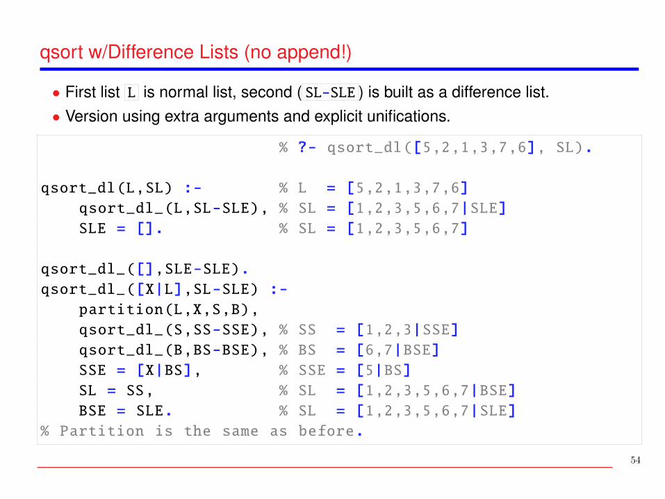
• First list L is normal list, second ( SL-SLE ) is built as a difference list.• Version using extra arguments and explicit unifications.
% ?- qsort_dl([5,2,1,3,7,6], SL).
qsort_dl(L,SL) :- % L = [5,2,1,3,7,6]
qsort_dl_(L,SL-SLE), % SL = [1,2,3,5,6,7|SLE]
SLE = []. % SL = [1,2,3,5,6,7]
qsort_dl_([],SLE-SLE).
qsort_dl_([X|L],SL-SLE) :-
partition(L,X,S,B),
qsort_dl_(S,SS-SSE), % SS = [1,2,3|SSE]
qsort_dl_(B,BS-BSE), % BS = [6,7|BSE]
SSE = [X|BS], % SSE = [5|BS]
SL = SS, % SL = [1,2,3,5,6,7|BSE]
BSE = SLE. % SL = [1,2,3,5,6,7|SLE]
% Partition is the same as before.
54

qsort w/Difference Lists (no append!)
• Version using extra arguments, in-place unifications.
qsort_dl(L,SL) :-
qsort_dl_(L,SL,[]).
qsort_dl_([],SLE,SLE).
qsort_dl_([X|L],SL,SLE) :-
partition(L,X,S,B),
qsort_dl_(S,SL,[X|BS]),
qsort_dl_(B,BS,SLE).
% Partition is the same as before.
55
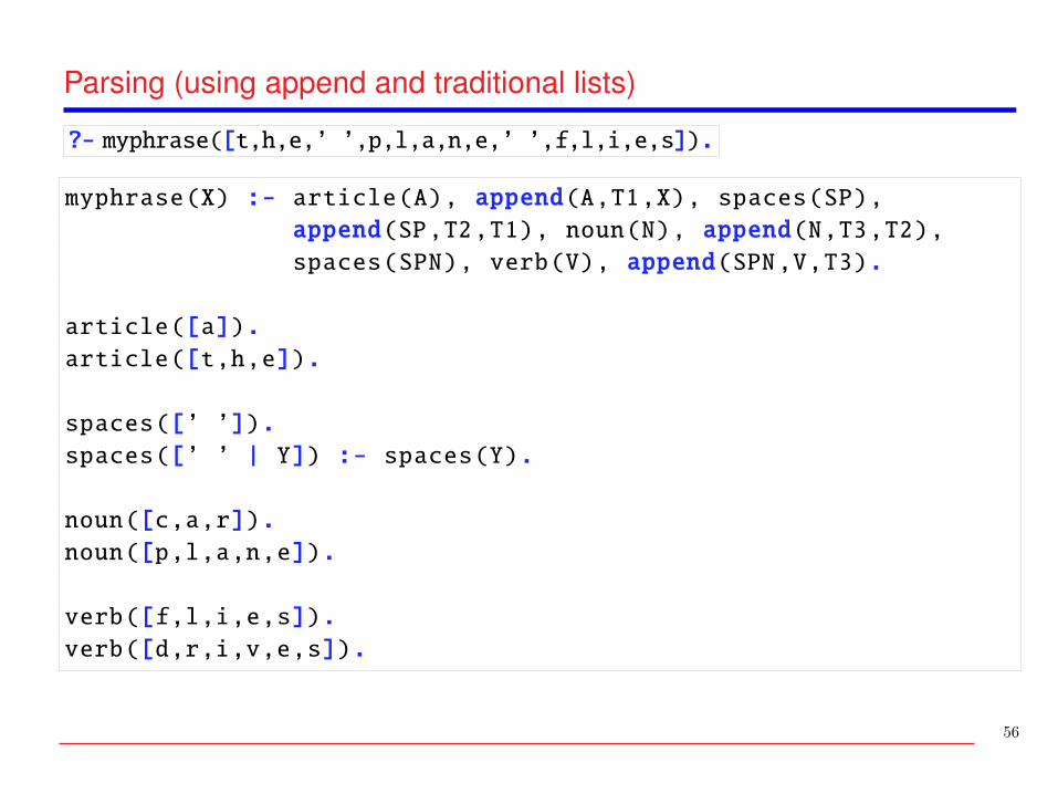
Parsing (using append and traditional lists)
?- myphrase([t,h,e,’ ’,p,l,a,n,e,’ ’,f,l,i,e,s]).
myphrase(X) :- article(A), append(A,T1,X), spaces(SP),
append(SP,T2,T1), noun(N), append(N,T3,T2),
spaces(SPN), verb(V), append(SPN,V,T3).
article([a]).
article([t,h,e]).
spaces([’ ’]).
spaces([’ ’ | Y]) :- spaces(Y).
noun([c,a,r]).
noun([p,l,a,n,e]).
verb([f,l,i,e,s]).
verb([d,r,i,v,e,s]).
56

Parsing (using standard clauses and difference lists)
?- myphrase([t,h,e,’ ’,p,l,a,n,e,’ ’,f,l,i,e,s],[]).
myphrase(X,CV) :-
article(X,CA), spaces(CA,CS1), noun(CS1,CN),
spaces(CN,CS2), verb(CS2,CV).
article([a|X],X).
article([t,h,e|X],X).
spaces([’ ’ | X],X).
spaces([’ ’ | Y],X) :- spaces(Y,X).
noun([c,a,r | X],X).
noun([p,l,a,n,e | X],X).
verb([f,l,i,e,s | X],X).
verb([d,r,i,v,e,s | X],X).
57

Parsing (same, using some string syntax)
?- myphrase("the plane flies",[]).
myphrase(X,CV) :-
article(X,CA), spaces(CA,CS1), noun(CS1,CN),
spaces(CN,CS2), verb(CS2,CV).
article("a" || X, X).
article("the" || X, X).
spaces(" " || X, X).
spaces(" " || Y, X) :- spaces(Y, X).
noun( "car" || X, X).
noun( "plane" || X, X).
verb( "flies" || X, X).
verb( "drives"|| X, X).
58
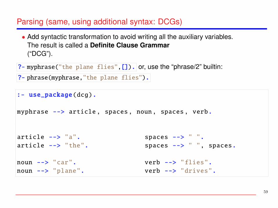
Parsing (same, using additional syntax: DCGs)
• Add syntactic transformation to avoid writing all the auxiliary variables.The result is called a Definite Clause Grammar(“DCG”).
?- myphrase("the plane flies",[]). or, use the “phrase/2” builtin:
?- phrase(myphrase,"the plane flies").
:- use_package(dcg).
myphrase --> article, spaces, noun, spaces, verb.
article --> "a". spaces --> " ".
article --> "the". spaces --> " ", spaces.
noun --> "car". verb --> "flies".
noun --> "plane". verb --> "drives".
59
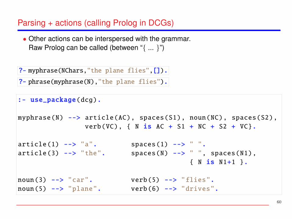
Parsing + actions (calling Prolog in DCGs)
• Other actions can be interspersed with the grammar.Raw Prolog can be called (between “{ ... }”)
?- myphrase(NChars,"the plane flies",[]).
?- phrase(myphrase(N),"the plane flies").
:- use_package(dcg).
myphrase(N) --> article(AC), spaces(S1), noun(NC), spaces(S2),
verb(VC), { N is AC + S1 + NC + S2 + VC}.
article(1) --> "a". spaces(1) --> " ".
article(3) --> "the". spaces(N) --> " ", spaces(N1),
{ N is N1+1 }.
noun(3) --> "car". verb(5) --> "flies".
noun(5) --> "plane". verb(6) --> "drives".
60
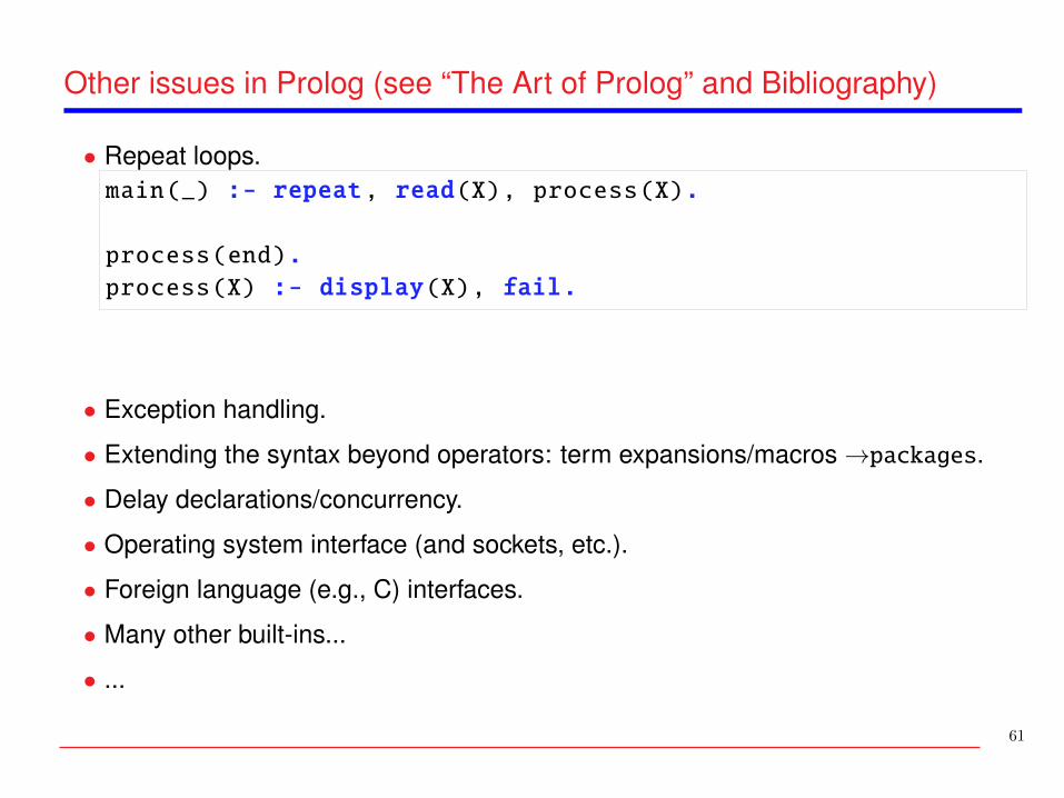
Other issues in Prolog (see “The Art of Prolog” and Bibliography)
• Repeat loops.main(_) :- repeat, read(X), process(X).
process(end).
process(X) :- display(X), fail.
• Exception handling.
• Extending the syntax beyond operators: term expansions/macros→packages.
• Delay declarations/concurrency.
• Operating system interface (and sockets, etc.).
• Foreign language (e.g., C) interfaces.
• Many other built-ins...
• ...
61
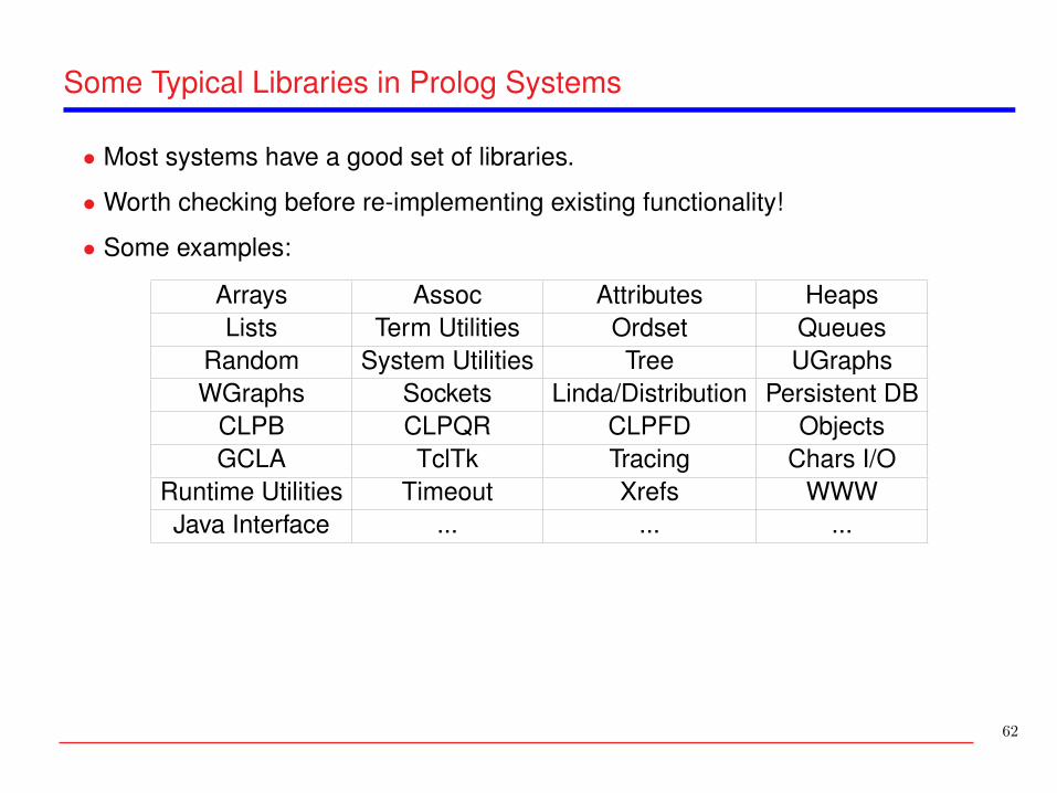
Some Typical Libraries in Prolog Systems
• Most systems have a good set of libraries.
• Worth checking before re-implementing existing functionality!
• Some examples:
Arrays Assoc Attributes HeapsLists Term Utilities Ordset Queues
Random System Utilities Tree UGraphsWGraphs Sockets Linda/Distribution Persistent DB
CLPB CLPQR CLPFD ObjectsGCLA TclTk Tracing Chars I/O
Runtime Utilities Timeout Xrefs WWWJava Interface ... ... ...
62

Some Additional Libraries and Extensions (Ciao)
Other systems may offer additional extensions. Some examples from Ciao:
• Other execution rules:
� Breadth-first, Iterative-deepening, Random, ...� Tabling� CASP (negation with multiple models)� Andorra (“determinate-first”) execution, fuzzy Prolog, ...
• Interfaces to other languages and systems:
� Interfaces to C, Java, JavaScript, Python, LLVM, ...� SQL database interface and persistent predicates� Web/HTML/XML/CGI programming (PiLLoW) / HTTP connectivity / JSON /
compilation to JavaScript ...� Interfaces to solvers (PPL, Mathematica, MiniSAT, Z3, Yikes, ...)� Graphviz, daVinci interfaces� Interfaces to Electron, wxWidgets, Tcl/Tk, VRML (ProVRML), ...� Calling Emacs from Prolog, etc.
63
Some Additional Libraries and Extensions (Ciao, Contd.)
• Many syntactic and semantic extensions:
� Functional notation� Higher-order� Terms with named arguments -records/feature terms� Multiple argument indexing� The script interpreter� Active modules (high-level distributed execution)� Concurrency/multithreading� Attributed variables� Object oriented programming� ...
64

Some Additional Libraries and Extensions (Ciao, Contd.)
• Constraint programming (CLP)
� rationals, reals, finite domains, ...� CHR (constraint handling rules), GeCode, ...
• Assertions:
� Regular types, Modes, Determinacy, etc.� Other properties� Run-time checking of assertions� Assertion-based unit tests and automatic test case generation� Compile-time property inference and assertion checking (CiaoPP).
• Additional programming support:
� Automatic documentation (LPdoc).� Partial evaluation, optimization, parallelization (CiaoPP).� ...
65