The Islamic University of GazaThe Islamic University of Gaza Deanery of Higher Studies Faculty of...
174
Transcript of The Islamic University of GazaThe Islamic University of Gaza Deanery of Higher Studies Faculty of...

The Islamic University of Gaza
Deanery of Higher Studies
Faculty of Commerce
Department of Business Administration
Predicting Corporate Failure
Using Cash Flow Statement Based Measures
“An Empirical Study on the Listed Companies in
the Palestine Exchange”
التنبؤ بتعثر الشركات عن طرق مقاس قائمة التذفق النقذي
"دراسة تطبقة على الشركات المذرجة ف بورصة فلسطن"
Prepared by
AHMED OMER ALOSTAZ
120120375
Supervised by
Prof. Fares M. Abu Mouamer
A Thesis Submitted in Partial Fulfillment of the Requirements for the Degree of MBA
2015 AD, 1436 AH


بسم ميحرلا نمحرلا هللا
يرفع الله الذين آمنوا منكم والذين أوتوا ﴿ ﴾العلم درجات والله بما تعملون خبير
صذق هللا العظم
(11:آية ،المجادلة)سورة

A
Dedication
Dedicated to my family specially my parents and to my lovely fiancé

B
Acknowledgement
Praise be to Allah, Lord of the Worlds, peace and prayers on the prophet
Muhammad peace be upon him.
I am very thankful to my supervisor, Professor Fares Abu Mouamer, for his
guidance, inspiration, encouragement, and invaluable support in positioning the
research from its beginning through its halfway to the final thesis.
I would like to thank Professor Yousif Ashour and Dr. Wael Thabet for their
generous acceptance for discussing my thesis and for their valuable advice.
A special thanks to Professor Samir Safi for his contribution in reviewing and
validating my statistical findings.
Also, I am very thankful to my professors whose taught me during the MBA
program as they greatly have enhanced my knowledge and ability to come up
with this work.
Finally, I would like to thank my family, colleagues and friends for their
encouragement and support throughout this the process.
C
Table of Contents
Dedication ......................................................................................................................... A
Acknowledgement ............................................................................................................ B
Table of Contents .............................................................................................................. C
List of Tables .................................................................................................................... G
List of Figures ..................................................................................................................... I
List of Abbreviations ......................................................................................................... J
Abstract ............................................................................................................................. K
Abstract in Arabic .............................................................................................................. L
1. Chapter One: Study Framework ............................................................................ 2
1.1 Introduction ........................................................................................................ 2
1.2 Problem Statement ............................................................................................. 3
1.3 Study Importance ............................................................................................... 4
1.4 Study Objectives ................................................................................................ 4
1.5 Study Variables .................................................................................................. 5
1.6 Study Hypotheses .............................................................................................. 6
1.7 Study Population ................................................................................................ 6
1.8 Study Limitations ............................................................................................... 7
1.9 Previous Studies ................................................................................................. 7 1.9.1 Arabic Studies ................................................................................................ 7 1.9.2 Foreign Studies ............................................................................................ 12
1.10 General Commentary on Previous Studies ...................................................... 17
1.11 The Originality/Value of This Study ............................................................... 18
2. Chapter Two: Literature Review ......................................................................... 21
2.1 An Overview of Corporate Failure and Bankruptcy ........................................ 21
1.2.2 Financial Distress, Failure, Bankruptcy and Liquidation Definitions ......... 21 2.1.2 Economic Distress and Financial Distress ................................................... 23 2.1.3 Financial Distress and Financial Failure ...................................................... 23
2.1.3.1 Financial Distress ................................................................................. 23 2.1.3.2 Financial Failure .................................................................................. 23
2.1.4 Causes of Business Failure .......................................................................... 24 2.1.4.1 Company-Specific Causes ................................................................... 24 2.1.4.2 External Causes .................................................................................... 28
D
2.1.5 Bankruptcy Process ...................................................................................... 30 2.1.6 Bankruptcy Around the World .................................................................... 30 2.1.7 Resolving Financial Distress ....................................................................... 34
2.1.7.1 Informal Methods of Resolving Financial Distress ............................. 34 2.1.7.2 Federal Bankruptcy Law ...................................................................... 35
2.1.7.3 Court- Formal Methods of Resolving Financial Distress .................... 36 2.1.8 Liquidation in Bankruptcy ........................................................................... 36 2.1.9 Failure Prediction Models ............................................................................ 37
2.1.9.1 Models for Predicting Bankruptcy ....................................................... 37 2.1.9.2 William Beaver Model ......................................................................... 38
2.1.9.3 Altman's Z-score .................................................................................. 38
2.2 Using Financial Analysis and Financial Ratios to Predict Failure .................. 41
2.2.1 The Statement of Cash Flow ........................................................................ 41 2.2.2 The Objectives of The Cash Flow Statement .............................................. 42
2.2.3 Steps to Prepare The Cash Flow Statement ................................................. 42 2.2.4 Definitions and Conventions of Accounting ............................................... 43
2.2.4.1 Going concern convention ................................................................... 43 2.2.4.2 Accruals basis ...................................................................................... 43
2.2.5 Quarterly Vs. Audited Financial Statement ................................................. 43
2.2.6 Techniques of Financial Statement Analysis ............................................... 44 2.2.7 Ratios Analysis ............................................................................................ 44
2.2.7.1 Ratio Analysis Definitions ................................................................... 44 2.2.7.2 Interested Parties .................................................................................. 45 2.2.7.3 Categories of Financial Ratios ............................................................. 46
2.2.7.4 Cash Flow Ratios ................................................................................. 48
2.2.7.5 Limitations of Ratio Analysis .............................................................. 50 1.1.2.2 Cautions About Using Ratio Analysis ................................................. 50 2.2.7.7 Using Accounting Ratios to Predict Financial Failure ........................ 51
2.3 Overview of Palestine Securities Exchange .................................................... 52 2.3.1 The Emergence and The Development of The PEX ................................... 52 2.3.2 The Objectives of Palestine Securities Exchange ........................................ 53
2.3.3 The Listed Companies in PEX ..................................................................... 53 2.3.4 Delisting Companies .................................................................................... 54
2.4 Multiple Linear Discriminant VS. Logistic Regression Model ....................... 55
2.4.1 Multiple Linear Discriminant Model ........................................................... 55
2.4.1.1 Multiple Linear Discriminant Model Definition ................................. 55
2.4.1.2 Justification for Not Using Multiple Linear Discriminant Model ....... 55 2.4.2 Linear Logistical Regression Model ............................................................ 56
2.4.2.1 Logistic Model Definition ................................................................... 56 2.4.2.2 Linear Logistic Regression Model ....................................................... 56 2.4.2.3 Interpretation of The Results ............................................................... 58
2.4.2.4 How The Model Might Fit The Data ................................................... 58
E
3. Chapter Three: Study Methodology and Data Analysis .................................... 60
3.1 Study Methodology .......................................................................................... 60 3.1.1 The Study Design ......................................................................................... 60 3.1.2 Statistical Tests ............................................................................................ 60 3.1.3 Data Collection ............................................................................................ 61
3.1.3.1 Secondary Data .................................................................................... 61 3.1.4 Study Population .......................................................................................... 61 3.1.5 Study Procedures ......................................................................................... 65 3.1.6 Predictor Variables ...................................................................................... 65
3.2 Data Analysis ................................................................................................... 68
3.2.1 Descriptive Statistics .................................................................................... 68
1.1.2.2 Firms Statistics ..................................................................................... 68
3.2.1.2 Ratios Statistics .................................................................................... 71 3.2.2 Testing for Normality .................................................................................. 81
3.2.3 Testing Hypothesis ...................................................................................... 86 3.2.3.1 Testing Hypothesis I ............................................................................ 86
3.2.3.2 Testing Hypothesis II ........................................................................... 90 3.2.3.3 Testing Hypothesis III ......................................................................... 97
4. Chapter Four: Study Results, Conclusions and Recommendations ............... 112
4.1 Study Results ................................................................................................. 112 4.1.1 Results of Testing Hypothesis I ................................................................. 112
4.1.1.1 Banking Sector ................................................................................... 112
4.1.1.2 Industrial Sector ................................................................................. 112
4.1.1.3 Insurance Sector ................................................................................. 112 4.1.1.4 Investing Sector ................................................................................. 113
4.1.1.5 Services Sector ................................................................................... 113 4.1.2 Results of Testing Hypothesis II ................................................................ 113
4.1.2.1 Banking Sector ................................................................................... 113
4.1.2.2 Industrial Sector ................................................................................. 113
4.1.2.3 Insurance Sector ................................................................................. 114 4.1.2.4 Investing Sector ................................................................................. 114
4.1.2.5 Services Sector ................................................................................... 114 4.1.3 Results of Testing Hypothesis III .............................................................. 114
4.1.3.1 Banking Sector ................................................................................... 114
4.1.3.2 Industrial Sector ................................................................................. 115 4.1.3.3 Insurance Sector ................................................................................. 115
4.1.3.4 Investing Sector ................................................................................. 116 4.1.3.5 Services Sector ................................................................................... 116
4.1.4 Other Results .............................................................................................. 117
4.2 Study Conclusions ......................................................................................... 118
4.3 Study Recommendations ............................................................................... 119
4.4 Research in Future ......................................................................................... 120
F
5. Bibliography ......................................................................................................... 121
6. Appendix (1) ......................................................................................................... 126
6.1 Observed Groups and Predicted Probabilities ............................................... 126
7. Appendix (2) ......................................................................................................... 132
7.1 Financial Ratios ............................................................................................. 132
7.2 Economic Sectors .......................................................................................... 144
7.3 Groups membership ....................................................................................... 147
7.4 Multicollinearity Test .................................................................................... 155
G
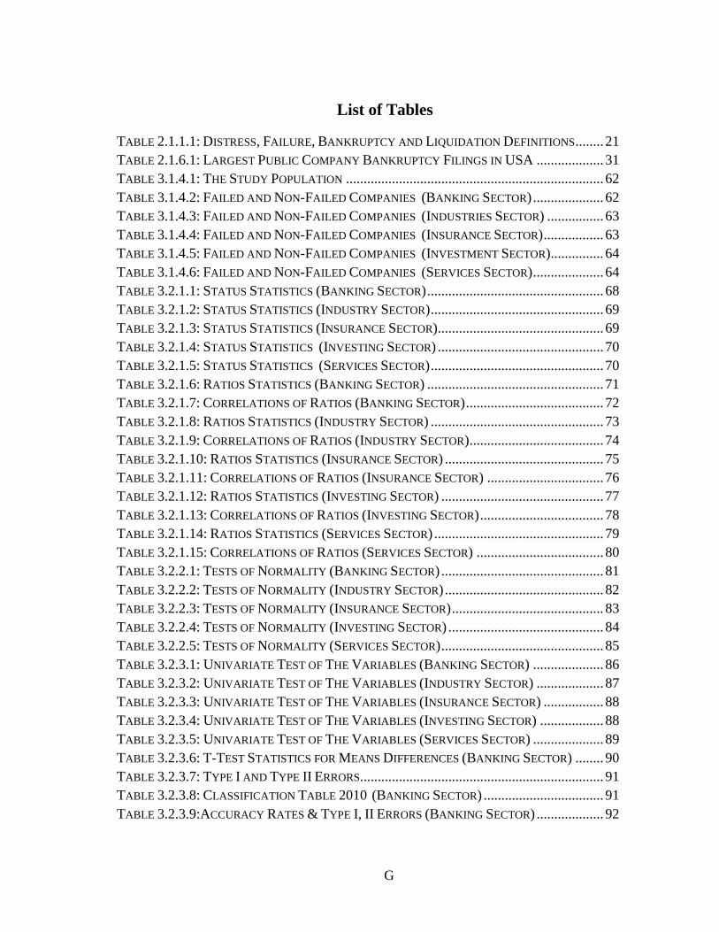
List of Tables
TABLE 2.1.1.1: DISTRESS, FAILURE, BANKRUPTCY AND LIQUIDATION DEFINITIONS ........ 21
TABLE 2.1.6.1: LARGEST PUBLIC COMPANY BANKRUPTCY FILINGS IN USA ................... 31
TABLE 3.1.4.1: THE STUDY POPULATION ......................................................................... 62
TABLE 3.1.4.2: FAILED AND NON-FAILED COMPANIES (BANKING SECTOR) .................... 62
TABLE 3.1.4.3: FAILED AND NON-FAILED COMPANIES (INDUSTRIES SECTOR) ................ 63
TABLE 3.1.4.4: FAILED AND NON-FAILED COMPANIES (INSURANCE SECTOR) ................. 63
TABLE 3.1.4.5: FAILED AND NON-FAILED COMPANIES (INVESTMENT SECTOR) ............... 64
TABLE 3.1.4.6: FAILED AND NON-FAILED COMPANIES (SERVICES SECTOR) .................... 64
TABLE 3.2.1.1: STATUS STATISTICS (BANKING SECTOR) .................................................. 68
TABLE 3.2.1.2: STATUS STATISTICS (INDUSTRY SECTOR) ................................................. 69
TABLE 3.2.1.3: STATUS STATISTICS (INSURANCE SECTOR)............................................... 69
TABLE 3.2.1.4: STATUS STATISTICS (INVESTING SECTOR) ............................................... 70
TABLE 3.2.1.5: STATUS STATISTICS (SERVICES SECTOR) ................................................. 70
TABLE 3.2.1.6: RATIOS STATISTICS (BANKING SECTOR) .................................................. 71
TABLE 3.2.1.7: CORRELATIONS OF RATIOS (BANKING SECTOR) ....................................... 72
TABLE 3.2.1.8: RATIOS STATISTICS (INDUSTRY SECTOR) ................................................. 73
TABLE 3.2.1.9: CORRELATIONS OF RATIOS (INDUSTRY SECTOR) ...................................... 74
TABLE 3.2.1.10: RATIOS STATISTICS (INSURANCE SECTOR) ............................................. 75
TABLE 3.2.1.11: CORRELATIONS OF RATIOS (INSURANCE SECTOR) ................................. 76
TABLE 3.2.1.12: RATIOS STATISTICS (INVESTING SECTOR) .............................................. 77
TABLE 3.2.1.13: CORRELATIONS OF RATIOS (INVESTING SECTOR) ................................... 78
TABLE 3.2.1.14: RATIOS STATISTICS (SERVICES SECTOR) ................................................ 79
TABLE 3.2.1.15: CORRELATIONS OF RATIOS (SERVICES SECTOR) .................................... 80
TABLE 3.2.2.1: TESTS OF NORMALITY (BANKING SECTOR) .............................................. 81
TABLE 3.2.2.2: TESTS OF NORMALITY (INDUSTRY SECTOR) ............................................. 82
TABLE 3.2.2.3: TESTS OF NORMALITY (INSURANCE SECTOR) ........................................... 83
TABLE 3.2.2.4: TESTS OF NORMALITY (INVESTING SECTOR) ............................................ 84
TABLE 3.2.2.5: TESTS OF NORMALITY (SERVICES SECTOR) .............................................. 85
TABLE 3.2.3.1: UNIVARIATE TEST OF THE VARIABLES (BANKING SECTOR) .................... 86
TABLE 3.2.3.2: UNIVARIATE TEST OF THE VARIABLES (INDUSTRY SECTOR) ................... 87
TABLE 3.2.3.3: UNIVARIATE TEST OF THE VARIABLES (INSURANCE SECTOR) ................. 88
TABLE 3.2.3.4: UNIVARIATE TEST OF THE VARIABLES (INVESTING SECTOR) .................. 88
TABLE 3.2.3.5: UNIVARIATE TEST OF THE VARIABLES (SERVICES SECTOR) .................... 89
TABLE 3.2.3.6: T-TEST STATISTICS FOR MEANS DIFFERENCES (BANKING SECTOR) ........ 90
TABLE 3.2.3.7: TYPE I AND TYPE II ERRORS..................................................................... 91
TABLE 3.2.3.8: CLASSIFICATION TABLE 2010 (BANKING SECTOR) .................................. 91
TABLE 3.2.3.9:ACCURACY RATES & TYPE I, II ERRORS (BANKING SECTOR) ................... 92
H
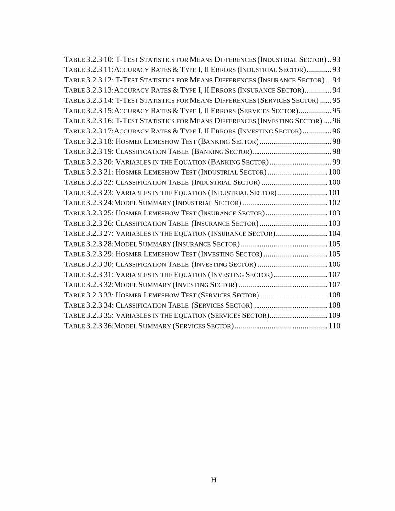
TABLE 3.2.3.10: T-TEST STATISTICS FOR MEANS DIFFERENCES (INDUSTRIAL SECTOR) .. 93
TABLE 3.2.3.11:ACCURACY RATES & TYPE I, II ERRORS (INDUSTRIAL SECTOR) ............. 93
TABLE 3.2.3.12: T-TEST STATISTICS FOR MEANS DIFFERENCES (INSURANCE SECTOR) ... 94
TABLE 3.2.3.13:ACCURACY RATES & TYPE I, II ERRORS (INSURANCE SECTOR) .............. 94
TABLE 3.2.3.14: T-TEST STATISTICS FOR MEANS DIFFERENCES (SERVICES SECTOR) ...... 95
TABLE 3.2.3.15:ACCURACY RATES & TYPE I, II ERRORS (SERVICES SECTOR) ................. 95
TABLE 3.2.3.16: T-TEST STATISTICS FOR MEANS DIFFERENCES (INVESTING SECTOR) .... 96
TABLE 3.2.3.17:ACCURACY RATES & TYPE I, II ERRORS (INVESTING SECTOR) ............... 96
TABLE 3.2.3.18: HOSMER LEMESHOW TEST (BANKING SECTOR) ..................................... 98
TABLE 3.2.3.19: CLASSIFICATION TABLE (BANKING SECTOR)......................................... 98
TABLE 3.2.3.20: VARIABLES IN THE EQUATION (BANKING SECTOR) ................................ 99
TABLE 3.2.3.21: HOSMER LEMESHOW TEST (INDUSTRIAL SECTOR) ............................... 100
TABLE 3.2.3.22: CLASSIFICATION TABLE (INDUSTRIAL SECTOR) .................................. 100
TABLE 3.2.3.23: VARIABLES IN THE EQUATION (INDUSTRIAL SECTOR) .......................... 101
TABLE 3.2.3.24:MODEL SUMMARY (INDUSTRIAL SECTOR) ............................................ 102
TABLE 3.2.3.25: HOSMER LEMESHOW TEST (INSURANCE SECTOR) ................................ 103
TABLE 3.2.3.26: CLASSIFICATION TABLE (INSURANCE SECTOR) ................................... 103
TABLE 3.2.3.27: VARIABLES IN THE EQUATION (INSURANCE SECTOR) ........................... 104
TABLE 3.2.3.28:MODEL SUMMARY (INSURANCE SECTOR) ............................................. 105
TABLE 3.2.3.29: HOSMER LEMESHOW TEST (INVESTING SECTOR) ................................. 105
TABLE 3.2.3.30: CLASSIFICATION TABLE (INVESTING SECTOR) .................................... 106
TABLE 3.2.3.31: VARIABLES IN THE EQUATION (INVESTING SECTOR) ............................ 107
TABLE 3.2.3.32:MODEL SUMMARY (INVESTING SECTOR) .............................................. 107
TABLE 3.2.3.33: HOSMER LEMESHOW TEST (SERVICES SECTOR) ................................... 108
TABLE 3.2.3.34: CLASSIFICATION TABLE (SERVICES SECTOR) ...................................... 108
TABLE 3.2.3.35: VARIABLES IN THE EQUATION (SERVICES SECTOR) .............................. 109
TABLE 3.2.3.36:MODEL SUMMARY (SERVICES SECTOR) ................................................ 110

I
List of Figures
FIGURE 2.1.4.1: EFFECT OF FINANCIAL LEVERAGE ON VALUE ......................................... 28
FIGURE 3.2.2.1: Q-Q PLOT OF X1. .................................................................................... 82
J
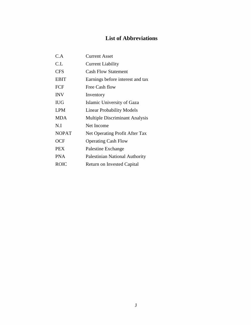
List of Abbreviations
C.A
C.L
CFS
EBIT
FCF
INV
IUG
LPM
MDA
N.I
NOPAT
OCF
PEX
PNA
ROIC
Current Asset
Current Liability
Cash Flow Statement
Earnings before interest and tax
Free Cash flow
Inventory
Islamic University of Gaza
Linear Probability Models
Multiple Discriminant Analysis
Net Income
Net Operating Profit After Tax
Operating Cash Flow
Palestine Exchange
Palestinian National Authority
Return on Invested Capital
K
Abstract
The purpose of this study is to test the predictive ability of the cash flow
statement ratios concerning corporate failure through developing a mathematical
model using financial ratios information. Financial ratios were derived from
financial statements publicly available from companies listed in Palestine
Exchange.
The study used the descriptive analytical approach to test the hypotheses and to
develop the models. Data was extracted over the past five years for 48 company
representing the 5-economic sectors in Palestine Exchange. Eleven predicting
variables were used, namely the Operating Cash Flow on Current Liabilities,
Cash Flow Coverage of Interest, Operating Cash Flow Margin, Operating Cash
Flow on Total Assets, Earning Quality, Quick Ratio, Operating Cash Flow on
Equity, Operating Cash Flow on Net Income, Operating Cash Flow on Current
Assets, Free Cash Flow on Current Liabilities and Operating Cash Flow on Free
Cash Flow.
The univariate analysis is used to test the first indicators of predictive variables
and the results showed that most variables can predict failure. Furthermore, the
study results showed that cash-flow ratios can discriminate firms into failed and
non-failed groups in both industrial and service sectors for 3-years before failure.
Finally the results showed many models that can be used to predict the failure for
each sector in the Palestine Exchange except for the banking sector. The results
showed that cash-flow ratios cannot discriminate between institutions in the
banking sector or predict its failure. However, the results showed in the industrial
sector that the most significant cash-flow ratios are the cash flow coverage of
interest ratio, operating cash-flow margin ratio and free cash flow on current
liabilities ratio. The investing sector showed that the most significant cash-flow
ratio is operating cash-flow on free cash-flow ratio. For insurance sector,
operating cash-flow on free cash-flow ratio was also the most significant one.
Finally for services sector the most significant ratios are operating cash-flow on
current liabilities ratio, operating cash-flow on total sales ratio, earning quality
ratio, quick ratio, operating cash-flow on equity ratio and operating cash-flow on
current assets ratio. The logistic model was able to discriminate between firms
and to predict the failure with an overall accuracy rate equal to (86%, 80%, 80%,
76%, 90%) for the banking, industrial, insurance, investing and service sectors
respectively.
The study recommends the investors, Palestine exchange management and
government agencies to use the models that have been reached to send early
warnings signals to the related parties in order to take the necessary corrective or
protective actions and to give more concern on cash flow statement based
measures in predicting corporate failure.

L
الملخص
من ىذه الدراسة ىو اختبار القدرة التنبؤية لنسب قائمة التدفقات النقدية المتعمقة اليدفحيث ،استخدام معمومات النسب الماليةبنموذج رياضي تطويرفشل الشركات من خالل ب
لشركات المدرجة في لمجميور من ا المتاحة القوائم الماليةتم اشتقاق النسب المالية من .بورصة فمسطين
، حيث تم وتطوير النماذج استخدمت الدراسة المنيج الوصفي التحميمي الختبار الفرضياتخمسة تمثل شركة لثمانية وأربعون استخراج البيانات عمى مدى السنوات الخمس الماضية
ىمو لمتنبؤ بالفشل مواأحد عشر متغير تم استخد. تصادية في بورصة فمسطينات اققطاعالتدفق النقدي التشغيمي عمى المطموبات المتداولة، تغطية التدفقات النقدية لمفائدة، ىامش
نسبة جودة ت، ة التشغيمية عمى إجمالي الموجوداالتدفقات النقدية التشغيمية، التدفقات النقديالسيولة السريعة، التدفق النقدي التشغيمي عمى حقوق المساىمين، التدفقات نسبة ،الدخل
التدفق النقدي التشغيمي عمى األصول الجارية، التدفق النقدية التشغيمية عمى صافي الدخل، .والتدفق النقدي التشغيمي عمى التدفق النقدي الحر النقدي الحر عمى المطموبات المتداولة
قدرة تنبؤية المؤشرات األولية من المتغيرات التي ليا الختبار استخداموتم األحاديالتحميل النتائج أن نسب أظيرتل أيضا التنبؤ بالفش ياوأظيرت النتائج أن معظم المتغيرات يمكن
اعة تميز بين الشركات في كل من قطاعي الصنالالتنبؤ و يايمكن قائمة التدفقات النقديةيمكن التي الفشل. أخيرا أظيرت النتائج العديد من النماذج منسنوات ثالث بلق والخدمات
النتائج أن نسب أظيرتحيث .فشل باستثناء نموذج القطاع المصرفيبالاستخداميا لمتنبؤ تتنبأ أن أو في القطاع المصرفيالمؤسسات ميز بينتستطيع أن تال النقديةالتدفقات
األكثر معنوية التدفقات النقديةأن نسب النتائج ي أظيرتفي القطاع الصناع بينما ،بالفشل نسبة التدفق النقدي التشغيمي و نسبة ىامش ة،مفائدلتغطية التدفقات النقدية نسبةىي
التدفقات نسب أكثر قطاع االستثمار فيو ،عمى المطموبات المتداولة صافي النقد الحربالنسبة لقطاع أما ،صافي النقد الحرعمى التدفق النقدي التشغيمي نسبة يأىمية ى النقديةايضا من اكثر نسب ىيصافي النقد الحر عمى التدفق النقدي التشغيمي نسبة التأمين
النسب األكثر معنوية ىي لقطاع الخدمات بالنسبة وأخيرا ،أىميةقائمة التدفقات النقدية

M
عمى إجمالي التشغيمي التدفق النقديعمى المطموبات المتداولة، التدفق النقدي التشغيميعمى حقوق التشغيميةالتدفقات النقدية ، نسبة السيولة السريعة، نسبة جودة الدخلالمبيعات، عمى األصول المتداولة. التدفقات النقدية التشغيميةو نسبة المساىمين
فشل بمعدل دقة يساوي بالكان النموذج الموجستي قادرا عمى التمييز بين الشركات والتنبؤ و التأمين، االستثمار ٪( لمقطاع المصرفي، الصناعي،08، ٪68٪، ٪68، ٪68، 68) عمى التوالي . يقطاع الخدماتالو
دارة والجيات الحكومية إلى استخدام النماذج بورصة فمسطينأوصى البحث المستثمرين، وا ت إلرسال إشارات تحذير مبكرة إلى األطراف ذامن قبل الباحث التي تم التوصل إلييا
، وزيادة االىتمام قبل الوقوع بالفشل أو الوقائية الالزمة العالجيةالعالقة التخاذ اإلجراءات التنبؤ بفشل الشركات. عمىبمؤشرات قائمة التدفق النقدي التي تساعد
1
Chapter One
General Framework of The Study
1.1 Introduction
1.2 Problem Statement
1.3 Study Importance
1.4 Study Objectives
1.5 Study Variables
1.6 Study Hypotheses
1.7 Study Population
1.8 Study Limitations
1.9 Previous Studies
1.10 General Commentary on Previous Studies
1.11 The Originality/Value of This Study
2
1. Chapter One: Study Framework
The Chapter one is about general framework of the study which includes
study problem, objectives, importance, variables, hypothesis, previous studies in
both foreign and Arabic studies, general commentary on previous studies and
finally the originality of this study.
1.1 Introduction
Business failure is a worldwide problem and one of the most investigated
topics within corporate finance. Business failure is the situation that a firm
cannot pay lenders, suppliers, shareholders and employees there accruals.
Numerous business failure studies have been performed over time using
traditional statistical techniques and financial ratios as input variables, starting
from the seminal paper of Beaver (1966), which initially proposed using
financial ratios as a failure predictor in a univariate context, followed by that of
Altman (1968), which proposed a multivariate approach based on discriminant
analysis. A number of these studies examined whether cash flow improves the
prediction of business failure, this study will use cash flow measures to predict
business failure since there is need for reliable models that predict corporate
failure to enable the parties concerned to take either preventive or corrective
actions.
are many reasons for small business failure such as lack of experience,
insufficient capital, poor inventory management, over-investment in fixed assets,
poor credit arrangement management and unexpected growth (Ames, 2013).
One of the most significant threats for many businesses today, despite
their size and the nature of their operations, is insolvency, the factors that lead
businesses to failure vary. Many economists attribute the phenomenon to high
interest rates, recession-squeezed profits and heavy debt burdens. Furthermore,
industry-specific characteristics, such as government regulation and the nature of
operations, can contribute to a firm‘s financial distress (Charitou, Neophytou, &
Charalambous, 2004, p. 465).
Bankruptcy may be defined as a condition in which an organization is
unable to meet its debt obligations, or petitions a federal district court for either
reorganization of its debts or liquidation of its assets (Altman, 1993). Financial
distress, on the other hand, is defined as a low cash-flow state in which a firm
incurs losses without being insolvent (Purnanandam, 2008).
The terms ―bankruptcy‖, ―failure‖, ―insolvency‖, ―liquidation‖, ―loan
default‖, ―credit risk‖, ―corporate distress‖ and ―financial distress‖ have been
used in referring to similar failure concepts (Altman, 1993).
3
There are many parties affected by business failure like investors,
creditors, management, suppliers, employees and the auditors if they failed to
report about signals of business failure in their auditing report.
Bankruptcy as a phenomenon has been studied in a lot of countries and
we may also encounter several across-countries studies. United States, Canada,
Australia, Japan, China, Italy, United Kingdom are but a few of the countries
where the most eminent studies in this field are conducted. Fewer studies, if none
at all, are found in the developing countries (Palestine in specific) or in the
transition economies (Shkurti & Duraj, 2010, p. 37).
The Corporate failure have been identified based on experts viewpoint by
comparing the first group the non-failed companies which have not subject to
failure condition (judgmental) with the second group of companies that failed
and subject to failure condition, if the company has a negative OCF in two
consecutive years or more during the study period from 2010-2014.
1.2 Problem Statement
The companies in Palestine Exchange don‘t adopt financial failure
prediction models based on cash-flow based measures. The previous studies in
predicting business failure used financial ratios derived from accrual accounting-
based financial statements. Therefore, there is need to build corporate failure
prediction models based on cash-flow measures to detect the companies that have
liquidity problems in the Palestine Exchange.
According to (Ataiwiel, 2008) in his study ―The Extent to Which the
Banks Depend on the Financial Analysis to Predict Failure”, the results showed
that the commercial banks rely less on financial analysis in predicting financial
distress or financial failure.
According to (Ghusain, 2004) in her study ―The Use of Financial Ratios
to Predict Corporate Failure‖ the study talks that the contracting companies did
not use financial analysis in predicting financial failure.
According to (Bhandari & Iyer, 2013, p. 667), most models used to
predict business failure used data derived from accrual accounting-based
financial statements namely the balance sheet and the income statement. Very
few studies used data from cash flow statement (CFS), or used any ratios based
on information in CFS.
The objective of this study is to explore the effect of cash flow statement
based measures in prediction of corporate failure in Palestine Exchange .
Therefore, the study main question is: Can cash flow ratios predict
corporate financial failure for each sector in the Palestine Exchange?
4
1.3 Study Importance
A. The financial intermediation offices in the PEX will benefit from the
models that have been reached by the researcher for each sector in the
PEX as it facilitates the assessment of companies‘ performance in
addition to predicting the possibility of business failure and to send early
warning signals to take corrective or preventive actions.
B. The investors will benefit from the models that have been reached for
each sector to help them in avoiding risky investments and reduce the risk
of losing their money in the PEX.
C. The government agencies will benefit from the models that have been
reached for detecting companies that may bankrupt in the future in order
to help them in avoiding financial crises in the PEX and maintain
economic stability.
D. The auditors will benefit from of the models that have been reached in
assessing company‘s ability to continue as a ―going concern‖.
E. Creditors and suppliers will benefit from the models that have been
reached to assess the liquidity position of the debtor firm.
F. This study content and findings can enrich the researcher‘s knowledge
and increase his experience in Palestine Exchange moreover increase the
researcher opportunities in developing his academic and professional
career.
1.4 Study Objectives
The main goal of this study is to test the ability of the CFS ratios to
predict corporate failure and to discriminate between failed and non-failed
companies for each sector in Palestine Exchange.
Other study objectives are:
A. Identifying significant CFS measures that can predict financial failure in
the PEX.
B. Test the ability of the CFS ratios to discriminate between failed and non-
failed companies before four years of failure incident in the PEX.
5
C. Develop a standard model utilizing CFS ratios able to discriminate
between healthy and failed companies for each sector in the PEX.
D. Provide some suggestions and recommendations to give more concern in
the use of cash flow statement based measures in predicting business
failure in the PEX.
1.5 Study Variables
First: Dependent Variable:
Corporate failure in Palestine Exchange which is a dummy variable that has two
values, (Y=0) for failed companies and (Y=1) for non-failed companies.
Second: Independent Variables:
Independent variables include mostly cash flow ratios.
Operating cash flow on current liabilities (OCF/CL).
Cash flow coverage of interest (OCF + INTREST + TAX/INT).
Operating cash flow margin (OCF/Sales).
Operating cash flow return on total assets (OCF/Asset).
Earning quality (EBIT/OCF).
Quick ratio or acid-test ratio (CA-INV)/CL.
Operating Cash flow on Equity (OCF/EQUITY).
Operating Cash flow on Net Income (OCF/N.I).
Operating Cash flow on Current Assets (OCF/C.A).
Free Cash Flow on Current Liabilities (FCF/C.L).
Operating Cash flow on Free Cash Flow (OCF/FCF).
After reviewing previous studies the researcher will use CFS ratios which
were used by (Bhandari & Iyer, 2013), (Matar & Obaidat, 2007), (Rodgers,
2013) and others. There are 33 type of cash flow ratios were used by researchers,
the most significant cash flows ratios that found in the results of the previous
studies will be used in this study.
6
1.6 Study Hypotheses
I. There are differences in cash-flow ratios between failed and non-failed
companies in PEX.
II. CFS ratios discriminate between failed and non-failed companies in the first,
second, third and fourth years respectively before failure incident in PEX.
III. The following financial ratios in the proposed developed model can predict
financial failure in PEX:
Operating cash flow on current liabilities (OCF/CL).
Cash flow coverage of interest (OCF + INTREST + TAX/INT).
Operating cash flow margin (OCF/Sales).
Operating cash flow return on total assets (OCF/Asset).
Earning quality (EBIT/OCF).
Quick ratio or acid-test ratio (CA-INV)/CL.
Operating Cash flow on Equity (OCF/EQUITY).
Operating Cash flow on Net Income (OCF/N.I).
Operating Cash flow on Current Assets (OCF/C.A).
Free Cash Flow on Current Liabilities (FCF/C.L).
Operating Cash flow on Free Cash Flow (OCF/FCF).
1.7 Study Population
The study population include all public listed companies in the Palestine
Exchange that representing five economic sectors for (48) financial institution
classified until the end of 2014. The study population was classified into two
groups, the first group the non-failed companies which have not subject to failure
condition (judgmental)1, the second group of companies that failed and subject to
failure condition, if the company has a negative OCF in two consecutive years or
more during the study period from (2010 to 2014). The fifth year is considered
the failure year.
1 The failure condition has been identified based on reviewing past studies and literatures also
based on experts‘ viewpoints.
7
1.8 Study Limitations
A. Limit the scope of this study in assessing the impact of only financial
ratios on the ability of companies to continue, while there are factors or
non-financial variables also affect their ability to continue. Such as: the
quality of management and the company activity nature and general
market, political and economic conditions surrounding the company.
B. The need for Palestine Exchange management in addition to the financial
intermediation offices to issue financial failure standard in order to guide
companies and researchers in identifying failed companies as there is
failure standard in other foreign stock exchanges.
C. This study covering the time period from 2010-2014 through the analysis
of financial statements over the past five years.
1.9 Previous Studies
A number of published researches/papers in certified journals are viewed
for the purpose of this study, focusing on using financial ratios for different
purposes. There are a few Palestinian and Arab papers on the topic, the study
depends highly on the foreign researches that match study purposes. The
researcher will begin with Arabic studies followed by foreign studies and finally
report general commentary on previous studies.
1.9.1 Arabic Studies
(AbuMoamer, 2014)
“Corporate Bankruptcy Prediction and Equity Returns in Palestinian Banks”
This study aims at finding the best set of financial ratios that can be used
to predict the failure of banking institutions and separate between failed and non-
failed ones in order to identify the conditions of those institutions earlier,
allowing interested parties and regulators to intervene to take appropriate
corrective action on time. The researcher used Multiple Linear Discriminant
Analysis (Stepwise Analysis) to find the best set of financial indicators that can
be used in building this model so that it can discriminate between the failed and
non-failed banking institutions before two years of failing. Financial ratios have
been calculated for a sample of eight banks, half of them failed and the other half
is not and that‘s for the period between the years (2007-2011). The following
proposed model was reached: Z =326.940A8 +37.810A11- 14.905A1-7.261A22-
2.347. Test of the model has been done by using financial ratios derived from the
sample data analysis and it was found to be able to predict the failure and
discriminate between failed and non-failed banking institutions with accuracy Of
(75%, 75%, 62.5%) in the first, third and fourth years respectively before failure.
8
(Alkhatib & Al Bzour, 2011)
“Predicting Corporate Bankruptcy of Jordanian Listed Companies: Using
Altman and Kida Models”
The purpose of this study is to explore the effect of financial ratios in
bankruptcy prediction of Jordanian listed companies through the use of Altman
and Kida models. Researchers used Altman and Kida models on the sample
companies in both service and industrial sectors. The study sample was including
non-financial service and industrial companies for the years 1990-2006.
Researchers excluded the banking, insurance and finance sectors from the study
because they apply certain disclosure requirements. Altman and Kida models
were applied on the sample companies in both service and industrial sectors. The
research results showed that of the two models, Altman's model has an advantage
in bankruptcy prediction with a 93.8% average predictive ability of the five years
prior to the liquidation incident, while the average for Kida's model is 69%. The
outcome of the analyses shows that Jordanian listed companies may not be using
such models in their financial and credit analyses. Researchers main
recommendation is that the best for Jordanian companies that they should at least
apply one of these models with high credibility for predicting corporate
bankruptcy.
(Rammo & Al-Wattar, 2010)
“Using Financial Analysis Techniques to Predict the Failure of Contributing
Industrial Companies: A Study of a Sample Consisting of Iraqi Contributing
Industrial Companies Listed in Iraqi Stock Market”
The present research aims at finding a reliable technique for failure
prediction through applying the Altman Model to a number of Iraqi
contributing companies. The importance of the research has come from the
importance of the failure subject through many parties related to the company.
The research problem exists in that the Iraqi shareholding companies, investors
and other parties are not aware of risks that lead the companies to failure in the
future. The model was applied on a sample consisted of (17) Iraqi shareholding
company after obtaining the necessary information about them. Several
findings were attained; the most important of which is Altman Model‘s
accuracy in predicting the failure of Iraqi companies. The study concluded that
Altman Model for predicting failure should be adopted as a reliable technique
in financial analysis when evaluating the performance of companies.
(Ataiwiel, 2008)
“The Extent to Which the Banks Depend on the Financial Analysis to Predict
Failure: An Empirical Study on the National Commercial Banks in the Gaza
Strip”
9
The purpose of this thesis is to identify the adoption extent of the national
commercial banks on financial analysis to predict failure. The researcher
conducted empirical study applied on (65) employees working in banks which
have already been identified earlier. Also, the method of comprehensive survey
has been used. The results showed that national commercial banks rely on
financial analysis significantly, the banks focus to use financial analysis
significantly to evaluate performance and decision making, the banks rely less on
financial analysis in predicting financial distress or financial failure, banks not
interested in giving courses in staff development in the area of predicting failure,
the national commercial banks do not use models to predict financial distress
effectively.
(Matar & Obaidat, 2007)
“The Role of Cash Flow Ratios in Improving the Accuracy of Models Based on
Accrual Ratios to Predict the Financial Failure of Jordanian Industrial
Companies Shareholders”
The purpose of this study is to identify the role of cash flow ratios in
improving the accuracy ability of the traditional models which are used to predict
the financial failure of Jordanian industrial companies as a going concern.
Researchers used Discriminant Analysis to design a mathematical model based
on 30 accrual ratios which were mostly used in related previous studies, on a
sample of (36) companies, half of them faced bankruptcy and the other half
continued, for the period which extended from 1989 to 2001. Also, the same
analysis, sample, and period were used to design another model based on (23)
cash flow ratios in addition to the previous accrual ratios. After that, each model
was tested on a sample of (37) companies, three of which faced bankruptcy and
the others continued, for the period which extended from 2002 to 2005. The
findings of the study revealed that the cash flow ratios improve the prediction
ability of the models of accrual ratios in regard to the evaluation of Jordanian
industrial companies as a going concern.
(Enshassi, Al-Hallaq, & Mohamed, 2006)
“Causes of Contractor's Business Failure in Developing Countries: The Case
of Palestine”
The objectives of this paper are to report on a research study which aims
at exploring the causes of contractor's business failure in Palestine, and
investigating their severity from the contractor's point of view. Researchers used
a total of 56 factors that may lead to contractors' business failure were identified
through a detailed literature review of relevant research studies. The study's
results shows that the main causes of business failure were delay in collecting
debt from clients (donors), border closure, heavy dependence on bank loans and
payment of high interest on these loans, lack of capital, absence of industry
10
regulations, low profit margin due to high competition, awarding contracts by
client to the lowest bidder, and lack of experience in contract management. The
research main recommendations to the Palestinian National Authority (PNA) and
local contractors are the PNA should take the risk when donors delay the debts of
the contractors, since most contracting companies in the Gaza Strip are small size
with lack of capital, the PNA should establish proper industry regulations and
suggest the appropriate mechanism for their enforcement, the PNA should
connect the contract price with the price index and the PNA should conduct
continuous training program, with cooperation of Palestinian Contractor Union
and universities in order to improve managerial and financial practice of local
contractors, tenders must be awarded to the best respondent bid with accurate
cost estimate and not necessarily to the lowest bidders, contracting companies
should not increase the number of projects that cannot be controlled, contracting
companies should consider political and business environment risk in their
estimate and contracting companies should improve their managerial and
financial abilities and practice in order to meet the challenge.
(Rugby, 2006)
“The Use of Financial Ratios to Predict Failure of Jordanian Public
Shareholding Companies Using Discriminant and Logit Analysis”
This study aims to use financial ratios by using discriminant and
logistical analysis methods to build statistical models to predict the failure of
listed public shareholding companies in the financial market. The researcher used
a sample of 26 pairs of failed and successful companies that covers the period
from 1991 to 2002 and the researcher has used 25 financial ratio that measures
the liquidity, profitability, leverage and activity. The results showed that the
discriminant model and logistic model were able to predict the failure of
companies one year before it happens with accuracy equal to 96%. Also, to
verify the external accuracy of these models, Jackknife approach was used and
showed that the results that have been reached were accurate. The researcher
mentioned that the ability of these models to predict have decreased as they were
in other studies, starting from the second year to the fifth year before the failure
year.
(Ghusain, 2004)
“The Use of Financial Ratios to Predict Corporate Failure: Empirical Study
on the Construction Sector in the Gaza Strip”
The purpose of this thesis is to develop model that can be used to predict
the failure of the construction sector companies in the Gaza Strip. The researcher
used twenty two financial ratios were calculated for a sample of ten failed
companies and sixteen non-failed companies from financial statements for three
11
years 2000, 2001, 2002. These ratios were analyzed using the statistical method
known as the logistic regression to reach the best form of financial ratios that can
discriminate between the failed and nonfailed contracting companies.
The model was developed: Log odds (kind) = -1.92-4.788R3-
1.05R5+0.074R19+0.074R21. The model that was developed contained four
financial ratios: net working capital to total assets, the sales to total assets, the
debtor to the sales, debtor to current assets. The model managed to accurately re-
classify companies in the sample within two groups of failed and nonfailed
categories, where the accuracy in discriminating between the failed and nonfailed
contracting companies was 91.9% , 86.9% , 86.9% , in 2002 ,2001 and 2000
respectively. The results of this study were that the financial ratios can used to
predict company‘s performance.
(Ashour & El-Farra, 2002)
“Business Failure in the Gaza Strip Bankers and Business Experts'
Viewpoints”
This paper examines the problems of high business failure rate in the
Gaza Strip. It focuses on the factors, which contributed significantly to business
failure in Gaza. These factors include, ‗short of funds and lack of ability to
manage liquidity‘, dissatisfaction of banking services, ‗poor managerial practices
and lack of experience in running businesses‘, lack of understanding of the
concept of company, ‗shortage of raw materials and poor maintenance
procedures‘, and lack of understanding of the concept of marketing. The study
main recommendations to prevent failure are:
It is crucial to undertake further field studies on sub-sectoral levels, to define
more specifically suitable programs for vocational training and rehabilitation
for each sub-sector. The needs and wants of businesses should be clearly
identified. In addition, providing advice and consultations to businesses
would help in reducing bankruptcy rate.
Merger with a healthy company could help in reducing the bankruptcy rate in
Gaza. Large businesses are more likely to survive and grow compared to
small ones.
Improve universities‘ education in Gaza and developing interaction between
universities and local businesses. In addition, university recruitment terms
and conditions should be altered to encourage research and development of
local business environment.
Improve the efficiency of decision-making and managerial practices in
planning, cash-flow management, pricing and marketing, in order to improve
the efficiency and competitive position of Gaza‘s business firms.
12
1.9.2 Foreign Studies
(Quarcoo & Smedberg, 2014)
“The Road to Bankruptcy: A Study on Predicting Financial Distress in
Sweden”
This thesis aims to study whether cash flow ratios can predict corporate
financial distress in Sweden by employing multiple discriminant analysis. The
hypotheses were tested through means of accuracy and the Independent Samples
Test. Researchers used a proxy ratio in order to identify financial distress. The
proxy was the operating cash flow ratio. Also they used a sample consisted of
227 firms in total within the retail- and service industries. The time period of the
study covered 2000-2013. The study results showed that the proxy was unable to
separate firms into distressed and non-distressed groups, but rather classified all
firms as distressed. Furthermore, the other ratios also failed to do any
classification. Finally, they concluded that cash flow ratios cannot predict
corporate financial distress for retail and service companies in Sweden.
(Bhandari & Iyer, 2013)
“Predicting Business Failure Using Cash Flow Statement Based Measures”
This paper addressed business failure during the economic recession of
2008-2012 years in USA. The purpose of this paper is to build a new model to
predict business failure, using mostly cash flow statement based measures as
predictors variables and discriminant analysis technique. Researchers used a
sample of 100 firms and seven variables. A total of 50 ―failed‖ firms were
matched with 50 non-failed firms according to Standard Industrial Classification
(SIC) code and size. Researchers use financial statement data for the year prior to
failed year were pulled from COMPUSTAT database and they used seven
predictor variables were selected, namely Operating cash flow divided by current
liabilities, Cash flow coverage of interest, Operating cash flow margin, Operating
cash flow return on total assets, Earning quality, Quick ratio and Three-year sales
growth. Researchers used The SPSS-19 software to perform discriminant
analysis (DA). Research main conclusion was that the DA. Model classified 83.3
percent of original groups cases correctly. The cross-validated approach (Jack-
knife or leave-one-out method) correctly classified 79.5 percent of cases. Also,
the chi-square test of Wilks‘ lambda was significant at 0.000 level which means
the model as a whole performed very well in predicting business failure.
( Mazouz, Crane, & Gambre, 2012)
“The Impact of Cash Flow on Business Failure Analysis and Prediction”
The purpose of this study is to determine whether cash flow impacts
business failure prediction using a neural network. The Researchers used a
sample of 114 failed and 114 non-failed manufacturing firms selected from the
13
Compustat database, accrual-based and cash flow-based neural network models
were developed utilizing financial ratios as input variables. Also, a Z-test was
performed to test for significance of any difference at the 0.05 level between the
classification results of the two models. The research results showed that the
accrual-based model correctly classified 92.55% of firms overall in a training
sample and 77.5% of firms overall in a holdout sample and the cash flow-based
model correctly classified 94.15% of firms overall in a training sample and
82.5% of firms overall in a holdout sample, moreover the cash flow-based neural
network model outperformed the accrual-based neural network model and the
results of the Z-test revealed that the difference in classification accuracies
between the two models was not significant. This study does not provide
evidence that cash flow improves business failure prediction.
(Hines, Kreuze, & Langsam, 2011)
“An analysis of Lehman Brothers bankruptcy and Repo 105 transactions”
The purpose of this paper is to investigate the bankruptcy of Lehman
Brothers, with particular focus on its use of Repo 105 transactions. The
researchers showed that the use of the Lehman‘s bankruptcy report produced in
part by Anton R. Valukas was used as a basis to explain how Lehman maintained
acceptable leverage ratios through the use of Repo 105 transactions to paint a
better picture of its financial position than actually existed. The study concludes
that Lehman‘s accounting method choice disguised its real problems, perhaps
long enough for bankruptcy to become the only option. The main research
conclusion is that Lehman‘s bankruptcy becomes part of a growing history of
business failures where accounting principles have become the focus. The
researchers mentioned that the failure of Lehman reminds us that financial
reporting must remain transparent, allowing users to make informed decisions
with confidence.
(Amendola, Bisogno, Restaino, & Sensini, 2011)
“Forecasting Corporate Bankruptcy: Empirical Evidence on Italian Data”
The aim of this paper is to investigate several aspects of bankruptcy
prediction within both theoretical and empirical frameworks. In particular, it has
focused on the comparison of different techniques used to forecast failure
through a balanced sample of companies within a geographical area (the
Campania region) located in the south of Italy. This paper‘s approach is to
compare different statistical techniques based on the analysis of financial data for
the prediction and diagnosis of the risk of bankruptcy. The paper investigates the
determinants of bankruptcy in a specific geographical area (Campania
region).The researchers relied on empirical evidence on a data-set of the annual
reports of a balanced sample of companies for a given time period has been
analysed. The researchers mentioned that findings aim to make a contribution to
14
current literature as well as to contribute to the elaboration of efficient prevention
and recovery strategies.
(Zaki, Bah, & Rao, 2011)
“Assessing Probabilities of Financial Distress of Banks in UAE”
The purpose of this research is to identify the main drivers of financial
institutions‘ financial distress in the UAE financial market. The paper estimates a
probability distress prediction model using the BankScope Database and the
annual reports of UAE financial institutions submitted to UAE Security
Exchange Authority. The paper also analyses the impact of macroeconomic
information for forecasting financial institutions‘ financial distress. The results
showed that fundamentals of financial institutions in terms of cost income ratio,
equity to total assets, total asset growth and ratio of loan loss reserve to gross
loans (all these variables with a lag of one year) positively impacted the
probability of financial distress in the next year. The researchers report that the
recent findings for emerging economies have cast some doubt on the usefulness
of macroeconomic information for financial institutions‘ risk assessment; similar
results are found for UAE financial institutions in predicting the probability of
financial distress.
(Chitnomrath, Evans, & Christopher, 2011)
“Corporate Governance and Post-Bankruptcy Reorganization Performance
Evidence from Thailand”
This research seeks to investigate the role of key corporate governance
mechanisms in determining a firm‘s post-bankruptcy performance following
reorganization. The study is based on agency theory and uses a unique sample of
111 filing companies whose reorganisation plans have been confirmed by the
Thai Central Bankruptcy Court during the period 1999-2002. The results indicate
that monitoring and incentive mechanisms are significant determinants of a
firm‘s post-bankruptcy performance. The key monitoring mechanism is
ownership concentration, measured by shares held by the largest shareholder,
whereas the critical incentive mechanisms are cash compensation and percentage
of common shares held by the plan administrator. The results indicate that these
mechanisms can mitigate agency problems in previously insolvent companies
and increase post-bankruptcy performance over a three year period.
(Dikmen, Birgonul, Ozorhon, & Sapci, 2010)
“Using Analytic Network Process to Assess Business Failure Risks of
Construction Firms”
The purpose of this study is to identify the determinants of business
failure in construction and to predict the failure likelihood of construction
15
companies by assessing their current situation based on both company-specific
and external factors. The researchers used the conceptual model designed based
on an extensive literature survey. Also, the analytical network process together
with the Delphi method was utilised to compute the importance weights of
variables on business failure through interviews and discussions with experts.
The applicability of the proposed model was tested on five companies to estimate
their failure likelihood by using the findings derived from the analysis. The
results suggest the importance of organisational and managerial factors,
including the efficiency of the value chain at the corporate level, the
appropriateness of organisational decisions, and the availability of intangible
resources for the survival of construction companies.
(Shkurti & Duraj, 2010)
“Using Multiple Discriminant Analysis in The Bankruptcy Prediction in
Albania A Study With The State-Owned Enterprises”
The purpose of this study is to apply the Multiple Discriminant Analysis
technique to study the bankruptcy of the state-owned enterprises in Albania. The
results showed that the discriminant function derived by this technique had an
overall accuracy rate by 94.6 percent when tested on the initial sample and 92.9
percent if tested using the cross-validation method. Also, the variables that best
discriminated between bankrupt and non-bankrupt firms were the level of
operating profitability and size of investments moreover they mentioned that
liquidity or cash flow variables were cited as important predictors of bankruptcy
and in other previous studies, did not result important. The main research
conclusion is that the economic profitability and good investment opportunities
are the main factors that affect the success of the state-owned enterprises in
Albania and they argue that often liquidity problems arise quite shortly before
the bankruptcy filing, thus it does not allow for inclusion among the early
predictors of bankruptcy.
(Kpodoh, 2010)
“Bankruptcy and Financial Distress Prediction in the Mobile Telecom
Industry”
The purpose of this thesis is to test Altman‘s Z-score prediction model
using sample data from the mobile telecommunication industry in Ghana. The
researched used quantitative and qualitative approach based on ‗modified single
case‘ design, primary data was collected using questionnaire survey methods,
whiles secondary data were mainly sourced from company annual financial
reports, industry regulators and industry analysts‘ reports. Also, the data was
analyzed using descriptive statistics, z-score analysis, financial ratio analysis and
trending, key solvency ratios were compared with industry averages. The z-
scores were compared with z-scores of other companies that went bankrupt in the

16
past. Corporate governance scores were compared to scores suggested by other
researchers as strong indicators of good corporate governance. The researcher
main conclusion was that the research findings confirmed the strength and ability
of the z-score model in predicting eminent business failure as it predicted
accurately the distress positions of the case companies. It also confirmed the
correlation between corporate governance and corporate failure. Finally,
companies operating in BOP markets ought to adopt and adapt the myriads of
marketing strategies available, especially for mobile telecommunication
operators, in order to be able to compete effectively and earn positive average
margin per user (AMPU) in the midst of declining average revenue per user
(ARPU) in the region.
(Charitou, Neophytou, & Charalambous, 2004)
“Predicting Corporate Failure: Empirical Evidence for the UK”
The main purpose of this study is to examine the incremental information content
of operating cash flows in predicting financial distress and develop reliable
failure prediction models for UK public industrial firms. Researchers used neural
networks and logit methodology to a dataset of fifty-one matched pairs of failed
and non-failed UK public industrial firms over the period 1988–97. They
validated the final models using an out-of-sample-period ex-ante test and the
Lachenbruch Jackknife procedure. The results indicate that a parsimonious
model that includes three financial variables, a cash flow, a profitability and a
financial leverage variable, yielded an overall correct classification accuracy of
83% one year prior to the failure. Finally, their models can be used to assist
investors, creditors, managers, auditors and regulatory agencies in the UK to
predict the probability of business failure.
17
1.10 General Commentary on Previous Studies
There are several studies addressed the business failure in more than one
aspect, there are different studies developed failure models for different sectors
and used various methods. Some research used the same model used by the
researcher and others did not. For example (Bhandari & Iyer, 2013), (Quarcoo &
Smedberg, 2014) and (Matar & Obaidat, 2007), ( Mazouz, Crane, & Gambre,
2012) used cash flow statement based measures as predictors variables which
have significant predictive power in business failure prediction. Most of these
empirical models used data derived from accrual accounting-based financial
statements such as (Zaki, Bah, & Rao, 2011), (Shkurti & Duraj, 2010), (Charitou,
Neophytou, & Charalambous, 2004), (AbuMoamer, 2014), (Alkhatib & Al
Bzour, 2011), (Rammo & Al-Wattar, 2010), (Ataiwiel, 2008), (Rugby, 2006) and
(Ghusain, 2004) which the researcher found these studies were important but
didn‘t outperformed cash flow measures in predicting business failure as the
results of the cash flow studies concluded. Discriminant analysis (DA) was most
widely used technique by (Enshassi, Al-Hallaq, & Mohamed, 2006), ( Mazouz,
Crane, & Gambre, 2012), (Shkurti & Duraj, 2010), (AbuMoamer, 2014),
(Amendola, Bisogno, Restaino, & Sensini, 2011), (Rugby, 2006), and (Ashour &
El-Farra, 2002). In addition to Altman and Kida‘s models were used by (Alkhatib
& Al Bzour, 2011), and (Rammo & Al-Wattar, 2010). Logistic models were used
by (Ghusain, 2004), (Charitou, Neophytou, & Charalambous, 2004), and (Rugby,
2006) since the sample that has been used was unbalanced sample of companies,
which also applied to this study. Others used Neural Network models such as (
Mazouz, Crane, & Gambre, 2012), (Charitou, Neophytou, & Charalambous,
2004). These authors have been evaluated, reviewed and compared their studies
on which attempted building of failure prediction models. A few attempts to use
cash flow-based data to build business failure prediction models.
After reviewing past studies the researcher concluded that the best model
for predicting corporate failure is by using cash flow based measures which
increase the predictive ability of the model before financial failure incident based
on the results of the previous studies of (Bhandari & Iyer, 2013), (Charitou,
Neophytou, & Charalambous, 2004), (Matar & Obaidat, 2007) and (Rodgers,
2013).
18
1.11 The Originality/Value of This Study
The present study differs from prior corporate failure studies in the following
respects:
A. Corporate failure is one of the most investigated topics within corporate
finance.
B. The sample companies are not industry specific in Palestine Exchange.
C. The eleven predictors were used by the researcher are logically justified.
D. Logistic regression model produces a more effective classification tool
than traditional multivariant discriminate analysis alone when evaluating
sets with two discrete dependent variables.
E. Most of the predictor variables use operating cash flow statement
information from the cash flow statement and not from accrual
accounting-based financial statements, which means the model is very
generic in nature.
F. A few articles, papers or studies have been addressing this issue in the
developing countries in general or in Palestine in specific
G. This study will make a contribution to current literature as well as to
contribute to the elaboration of efficient prevention and recovery
strategies.
H. This study represented a fundamental reference point for future
researches.
19
Study Content
This study includes four chapters, the study proposal with the previous studies
were presented in chapter one. The literatures review will be covered in four
sections in chapter two, the first section includes an overview of corporate failure
and bankruptcy, the second section will focus on financial analysis and financial
ratios to predict failure, the third section highlight the Palestine Exchange in
general and the fourth section will discuss the multiple discriminant model and
logistic model. The third chapter includes the study methodology with the data
analysis that performed by SPSS-21 software which considered the most
common software for social sciences. Finally the fourth chapter will show the
study results, conclusions and recommendations.
20
Chapter Two
Literature Review
2.1 An Overview of Corporate Failure and Bankruptcy
2.2 Financial Analysis and Financial Ratios to Predict Failure
2.3 Overview of Palestine Securities Exchange
2.4 Multiple Linear Discriminant Model VS. Linear Logistic
Regression Model
21
2. Chapter Two: Literature Review
The chapter two includes four sections, the first section presents an
overview of corporate failure and bankruptcy, the second section focus on
financial analysis and financial ratios to predict failure, the third section
highlights the Palestine Exchange in general and finally the four section discuss
in briefly MDA model and linear logistic model.
2.1 An Overview of Corporate Failure and Bankruptcy
Section one talks about financial failure definitions, causes of financial
distress either internal factors or external factors and a brief discussion of capital
structure theories. Also this section presents bankruptcy process, bankruptcy
around the world, methods of resolving financial distress, liquidity in bankruptcy
and finally failure prediction models.
2.1.1 Financial Distress, Failure, Bankruptcy and Liquidation Definitions
The terms ―bankruptcy‖, ―failure‖, ―insolvency‖, ―liquidation‖, ―loan
default‖, ―credit risk‖, ―corporate distress‖ and ―financial distress‖ have been
used in referring to similar failure concepts (Altman, 1993).
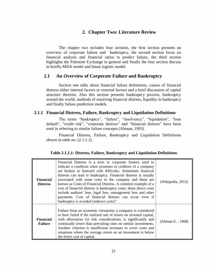
Financial Distress, Failure, Bankruptcy and Liquidation Definitions
shown in table no. (2.1.1.1).
Table 2.1.1.1: Distress, Failure, Bankruptcy and Liquidation Definitions
Financial
Distress
Financial Distress is a term in corporate finance used to
indicate a condition when promises to creditors of a company
are broken or honored with difficulty. Sometimes financial
distress can lead to bankruptcy. Financial distress is usually
associated with some costs to the company and these are
known as Costs of Financial Distress. A common example of a
cost of financial distress is bankruptcy costs; these direct costs
include auditors' fees, legal fees, management fees and other
payments. Cost of financial distress can occur even if
bankruptcy is avoided (indirect costs)‖.
(Wikipedia, 2015)
Financial
Failure
Failure from an economic viewpoint; a company is considered
to have failed if the realized rate of return on invested capital,
with allowances for risk considerations, is significantly and
continually lower than prevailing rates on similar investments.
Another criterion is insufficient revenues to cover costs and
situations where the average return on an investment is below
the firm's cost of capital.
(Altman E. , 1968)
22
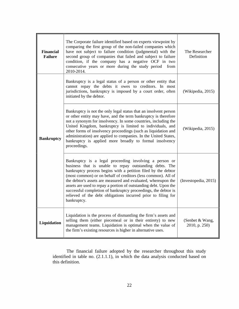
Financial
Failure
The Corporate failure identified based on experts viewpoint by
comparing the first group of the non-failed companies which
have not subject to failure condition (judgmental) with the
second group of companies that failed and subject to failure
condition, if the company has a negative OCF in two
consecutive years or more during the study period from
2010-2014.
The Researcher
Definition
Bankruptcy
Bankruptcy is a legal status of a person or other entity that
cannot repay the debts it owes to creditors. In most
jurisdictions, bankruptcy is imposed by a court order, often
initiated by the debtor.
(Wikipedia, 2015)
Bankruptcy is not the only legal status that an insolvent person
or other entity may have, and the term bankruptcy is therefore
not a synonym for insolvency. In some countries, including the
United Kingdom, bankruptcy is limited to individuals, and
other forms of insolvency proceedings (such as liquidation and
administration) are applied to companies. In the United States,
bankruptcy is applied more broadly to formal insolvency
proceedings.
(Wikipedia, 2015)
Bankruptcy is a legal proceeding involving a person or
business that is unable to repay outstanding debts. The
bankruptcy process begins with a petition filed by the debtor
(most common) or on behalf of creditors (less common). All of
the debtor's assets are measured and evaluated, whereupon the
assets are used to repay a portion of outstanding debt. Upon the
successful completion of bankruptcy proceedings, the debtor is
relieved of the debt obligations incurred prior to filing for
bankruptcy.
(Investopedia, 2015)
Liquidation
Liquidation is the process of dismantling the firm‘s assets and
selling them (either piecemeal or in their entirety) to new
management teams. Liquidation is optimal when the value of
the firm‘s existing resources is higher in alternative uses.
(Senbet & Wang,
2010, p. 250)
The financial failure adopted by the researcher throughout this study
identified in table no. (2.1.1.1), in which the data analysis conducted based on
this definition.
23
There are differences between bankruptcy and financial distress, in the
case of bankruptcy the debtor completely stopped payment of his debts, while
in the case of financial distress the debtor's funds are not sufficient to cover his
owed debts even if the total assets more than the total liabilities.
Bankruptcy may be defined as a condition in which an organization is
unable to meet its debt obligations, or petitions a federal district court for either
reorganization of its debts or liquidation of its assets (Altman, 1993). Financial
distress, on the other hand, is defined as a low cash-flow state in which a firm
incurs losses without being insolvent (Purnanandam, 2008).
Liquidation is the process of dismantling the firm‘s assets and selling
them (either piecemeal or in their entirety) to new management teams.
Liquidation is optimal when the value of the firm‘s existing resources is higher in
alternative uses (Senbet & Wang, 2010, p. 250).
There is difference between bankruptcy and liquidation both of the them
is independent and has separate events and costs.
A profitable firm with high leverage may remain viable as a going
concern, irrespective of bankruptcy, while an unprofitable firm may be liquidated
even if it has no debt in its capital structure (Senbet & Wang, 2010, p. 250).
Therefore, there are differences between economic distress and financial distress.
2.1.2 Economic Distress and Financial Distress
Financial distress means that the firm‘s promises to creditors are broken
or honored with difficulty. It is directly related to the firm‘s leverage decision.
Economic distress, however, means difficulties arising from the firm‘s
operational inefficiencies. It has no direct linkage to the firm‘s leverage (Senbet
& Wang, 2010, p. 249).
2.1.3 Financial Distress and Financial Failure
There are differences between financial distress and financial failure;
financial distress is a condition that precedes the financial failure but not
necessary followed by financial failure. We can distinguish between them
according to:
2.1.3.1 Financial Distress (Ghusain, 2004):
A. Low stock returns or retained.
B. Stop payment of obligations in maturity.
2.1.3.2 Financial Failure (Ghusain, 2004):
A. Stop completely of payment of obligations.
B. Stop engagement in any activity.
24
In the case of financial distress, there is no enough cash (negative OCF)
to cover short-term obligations and the net capital is positive. In the case
of financial failure, the net capital is negative and total liabilities more
than the total assets and the company completely unable to pay debts it‘s
owed to creditors.
2.1.4 Causes of Business Failure
There are many causes of business failure either by external factors or
(internal) company-specific factors such as managerial, financial, technical and
marketing causes.
A company‘s intrinsic value is the present value of its expected
future free cash flows. There are many factors that can cause this
value to decline. These factors include general economic
conditions, industry trends, and company-specific problems such as
shifting consumer tastes, obsolescent technology, and changing
demographics in existing retail locations. Financial factors, such as
too much debt and unexpected increases in interest rates, can also
cause business failures. The importance of the different factors
varies over time, and most business failures occur because a
number of factors combine to make the business unsustainable.
(Ehrhardt & Brigham, p. 870).
2.1.4.1 Company-Specific Causes (Internal Factors)
Business causes arise when the company‘s performance falls below
expectations due to lack of competiveness, operational issues, or poor
leadership. These arise as a result of poor decisions, bad timing, or just
bad luck. Financial causes arise either because the company's capital
structure is inappropriate given its level of business risk, or poor financial
decisions are made by management during the day-to-day operations
(Danilov, 2014, p. 15).
Most failures occur because a number of factors combine to make the
business unsustainable. Company specific factors can classify
according to:
I. Non-Financial (“Business”) Causes
A. The absence of specialized administrative and technical elements, the
existence of conflicts between members of top management, giving
priority to the special interests of the shareholders with the owners and
the wrong directions for management (Ghusain, 2004, p. 27).
25
B. The lack of competitiveness of the company's product or service in the
market. This can occur for a variety of reasons like the entry of new
competitors into the market, a lack of differentiation and pricing power,
or shifting consumer tastes. New or existing competitors may provide a
better product at the same price, or are able to price at below-market
levels due to cost leadership. Either way, customers are no longer willing
to purchase the company's offering. If management is not able to adapt
the product or service, sales will fall below forecasted levels and the
company will eventually fail (Danilov, 2014, p. 16).
C. Unexpected non-debt liabilities such as tort lawsuits or contract liabilities
represent another potential source of business failure. Tort claims - a
claim that a company has caused personal injury to another individual -
can arise various types of businesses, but have been most prevalent in
tobacco, silicon and asbestos related sectors. As a result of the potential
for large punitive damage awards, a class-action lawsuit can destabilize a
sound, profitable business and force it to seek bankruptcy protection
(Danilov, 2014, p. 17).
D. Conflict of interest arise as a result of incompatible objectives between
owners and the managers of the firm.
II. Financial Causes
Another cause of failure is financial failure which includes high financial
leverages, illiquidity due to working capital mismanagement, or high
operating leverage due to increased fixed costs.
A. Operating Leverage
The extent to which fixed costs are used in a firm‘s operations. In
business terminology, a high degree of operating leverage, other factors
held constant, implies that a relatively small change in sales results in a
large change in ROIC (Ehrhardt & Brigham, 2011).
High operating leverage implies that a relatively small change in sales
results in a relatively large change in EBIT, net operating profits after
taxes (NOPAT), and return on invested capital (ROIC). Other things held
constant, the higher a firm‘s fixed costs, the greater it‘s operating
leverage. Higher fixed costs are generally associated with (1) highly
automated, capital intensive firms; (2) businesses that employ highly
skilled workers who must be retained and paid even when sales are low;
and (3) firms with high product development costs that must be
maintained to complete on-going R&D projects (Ehrhardt & Brigham,
2011, p. 604).
26
The firms that rely highly on operating leverage which will not decline as
sales falls will increase its business risk and may lead eventually to
business failure.
B. Financial Leverage
Is the extent to which fixed-income securities (debt and preferred stock)
are used in a firm‘s capital structure. Financial risk is the added risk borne
by stockholders as a result of financial leverage (Ehrhardt & Brigham,
2011, p. 631) .
Interest and principal payments represent a fixed cost that raises the
company's breakeven point in the same manner as operating leverage,
thus increasing earnings variability (Danilov, 2014, p. 18).
High levels of debts represent high probability of bankruptcy, increasing
debts which mean increasing financial leverage will increase the risk of
the company of being unable to meet its financial obligations and for this
reason the cost of common equity will increase as well to compensate the
increase of business risk.
C. Capital Structure Theories
Additional debt increases the probability of bankruptcy. Capital structures
vary among firms within a given industry. There are many theories
regarding capital structures that will be highlighting in briefly by the
researcher.
Bankruptcy in the Modigliani-Miller World
The corollary of the MM theorem is that corporate bankruptcy is
inconsequential to firm value, since the investment decisions are
completely separable from the financing decisions. In the perfect and
frictionless MM world, the amount of corporate indebtedness has no
effect on the value of the firm‘s assets or on the risk of the total cash flow
stream generated by the firm‘s assets. The capital structure of the firm
simply determines how the total cash flow is partitioned between equity
holders and debt holders and thus the risk borne by each class of capital
providers. Bankruptcy is essentially a transfer of ownership from equity
holders to debt holders when the value of assets drops below the value of
debt. The complete separation between financing decisions and
investment decisions implies that there is no necessary linkage between
bankruptcy and the firm‘s operating performance (Senbet & Wang, 2010,
pp. 248-249).
Modigliani and Miller (1963) argue that the tax code favors debt over
equity financing by allowing the firm‘s interest expense to be deducted
from gross income for corporate tax purposes, but disallowing
deductibility of payments to equity holders (e.g., dividends are not tax
27
deductible on the personal account). Since an additional dollar of debt
generates the marginal benefit of a tax deduction without any offsetting
cost in this framework, the firm value is maximized by utilizing as much
debt as possible to finance corporate investment decisions (Senbet &
Wang, 2010, p. 250).
Trade-off Theory
The trade-off theory of leverage, in which firms trade off the benefits of
debt financing (favorable corporate tax treatment) against higher interest
rates and bankruptcy costs (Ehrhardt & Brigham, 2011, p. 613).
Although that the increase use of debt will increase the tax saving that the
company will benefit from it, also it will increase bankruptcy costs which
divided into two types: direct costs and indirect costs.
A. Direct Costs
Auditors' fees
Legal fees
Management fees
Other payments and accounting expenses that the company will
suffer when it incurred bankruptcy
B. Indirect costs
Lost customers who search for more stable suppliers
Reduction in productivity of managers and line workers who are
worried about their future,
Reduction in credit (i.e., accounts payable) offered by suppliers and
imposed high interest rates by the lenders.
According to the theory, the optimal level is reached when further
borrowing results in a PV of tax savings that is fully offset by the
increases in the PV of bankrupt cost (Danilov, 2014, p. 18).
As the Debt equity ratio (i.e. leverage) increases, there is a trade-off
between the interest tax shield and bankruptcy, causing an optimum
capital structure as shown in figure No. (2.1.4.1):
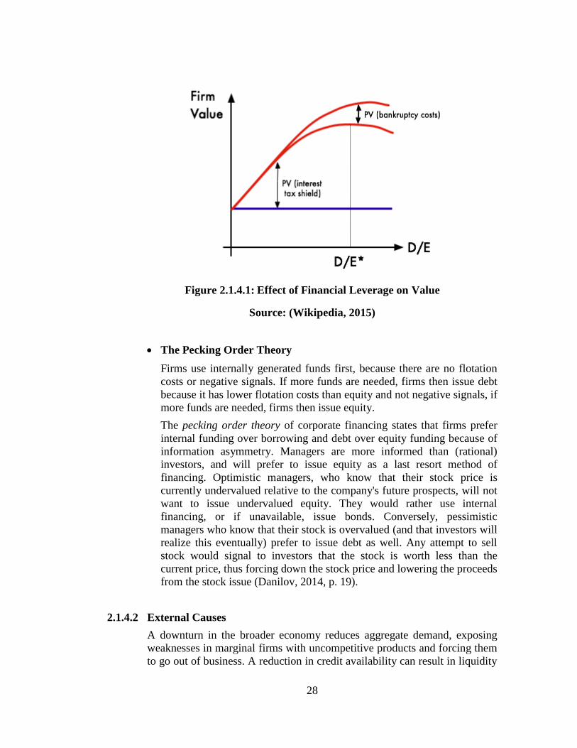
28
Figure 2.1.4.1: Effect of Financial Leverage on Value
Source: (Wikipedia, 2015)
The Pecking Order Theory
Firms use internally generated funds first, because there are no flotation
costs or negative signals. If more funds are needed, firms then issue debt
because it has lower flotation costs than equity and not negative signals, if
more funds are needed, firms then issue equity.
The pecking order theory of corporate financing states that firms prefer
internal funding over borrowing and debt over equity funding because of
information asymmetry. Managers are more informed than (rational)
investors, and will prefer to issue equity as a last resort method of
financing. Optimistic managers, who know that their stock price is
currently undervalued relative to the company's future prospects, will not
want to issue undervalued equity. They would rather use internal
financing, or if unavailable, issue bonds. Conversely, pessimistic
managers who know that their stock is overvalued (and that investors will
realize this eventually) prefer to issue debt as well. Any attempt to sell
stock would signal to investors that the stock is worth less than the
current price, thus forcing down the stock price and lowering the proceeds
from the stock issue (Danilov, 2014, p. 19).
2.1.4.2 External Causes
A downturn in the broader economy reduces aggregate demand, exposing
weaknesses in marginal firms with uncompetitive products and forcing them
to go out of business. A reduction in credit availability can result in liquidity
29
problems for over-levered companies that would have continued to operate
otherwise. While most macroeconomic factors are interrelated, aggregate
measures and such as GNP growth, money supply, financial market
performance and number new business starts seem to be correlated with
increased rates of corporate failure and financial distress (Danilov, 2014, p.
30).
Also inflation, increase prices of raw materials, production materials, power
prices, increase costs and lower profits or increase losses are causes of
business failure.
Fluctuations in exchange rates increase the value of debts the companies
incurred which may results to business failure.
Technological changing and the new products entered the markets and
changing human capital may leads to business failure.
There are many studies report and concluded the business failure causes, the
researcher will mention some of them:
(Ashour & El-Farra, 2002, p. 2) Summarized the causes of business failure
as follow:
Short of funds and lack of ability to manage liquidity.
Dissatisfaction of banking services.
Poor managerial practices and lack of experience in running
businesses.
Lack of understanding of the concept of company.
Shortage of raw materials.
Poor maintenance procedures.
Lack of understanding of the concept of marketing.
Also (Enshassi, Al-Hallaq, & Mohamed, 2006, p. 1) in their study concluded
that the main causes of business failure were:
Delay in collecting debt from clients (donors).
Border closure.
Heavy dependence on bank loans and payment of high interest on
these loans.
Lack of capital.
Absence of industry regulations.
Low profit margin due to high competition.
Awarding contracts by client to the lowest bidder.
Lack of experience in contract field.
30
2.1.5 Bankruptcy Process
When a company with financial obligations to outside creditors
becomes insolvent, its creditors have several options. They can either
negotiate directly with the company (i.e. the debtor) to turn things around or
choose to pursue legal action against the company. A secured creditor, one
that has a claim (i.e. obligation) that is backed by a specific asset, can move
to seize the asset and sell it to fulfill the obligation owed to it by the debtor.
An unsecured creditor can pursue legal action by suing the debtor to obtain a
lien on an asset that it could then seize and sell to fulfill its obligation.
Alternatively, instead of pursuing non- bankruptcy legal remedies, the
creditors can collectively force the debtor into a bankruptcy proceeding.
(The company can also voluntarily enter bankruptcy proceedings in order to
seek the court's protection from creditors) (Danilov, 2014, p. 10).
2.1.6 Bankruptcy Around the World2
In this part the researcher will highlight bankruptcy around the world
especially in United States of America (USA) where the most large and famous
firms have filing for bankruptcy.
Lehman Brothers, Washington Mutual, Chrysler, and General Motors all
filed for bankruptcy protection during the global economic crisis. What did these
four filings have in common with Australia? At the time of filings, the
companies‘ assets totaled over $1.1 trillion dollars, which is about the same size
as Australia‘s annual gross domestic product. With $691 billion in assets,
Lehman Brothers holds the record for the largest bankruptcy filing in history.
Lehman Brothers had not emerged from bankruptcy when we wrote this (August
2009), but it is unlikely that Lehman Brothers will again operate as a company.
Most of its operations and assets have been liquidated and sold piecemeal to
other companies, including Barclays (Ehrhardt & Brigham, 2011, p. 869).
When GM filed for bankruptcy on June 1, it became the largest
manufacturer in U.S. history to fail. When GM emerged from bankruptcy 40
days later, the U.S. government owned 60.8% of the equity in the ―new‖ GM,
with the remaining equity owned by the Canadian government (11.7%), the
UAW employee health care trust (17.5%), and former bondholders (10%). Notice
that nothing was left for former stockholders (Ehrhardt & Brigham, 2011, p.
869).
Bankruptcy is not occurring only for small firms but also big firms have
filing for bankruptcy in the period of 2008-2009 as a result of global economic
2 To read more about Bankrupt firms you can access http://www.instantshift.com/2010/02/03/22-
largest-bankruptcies-in-world-history/
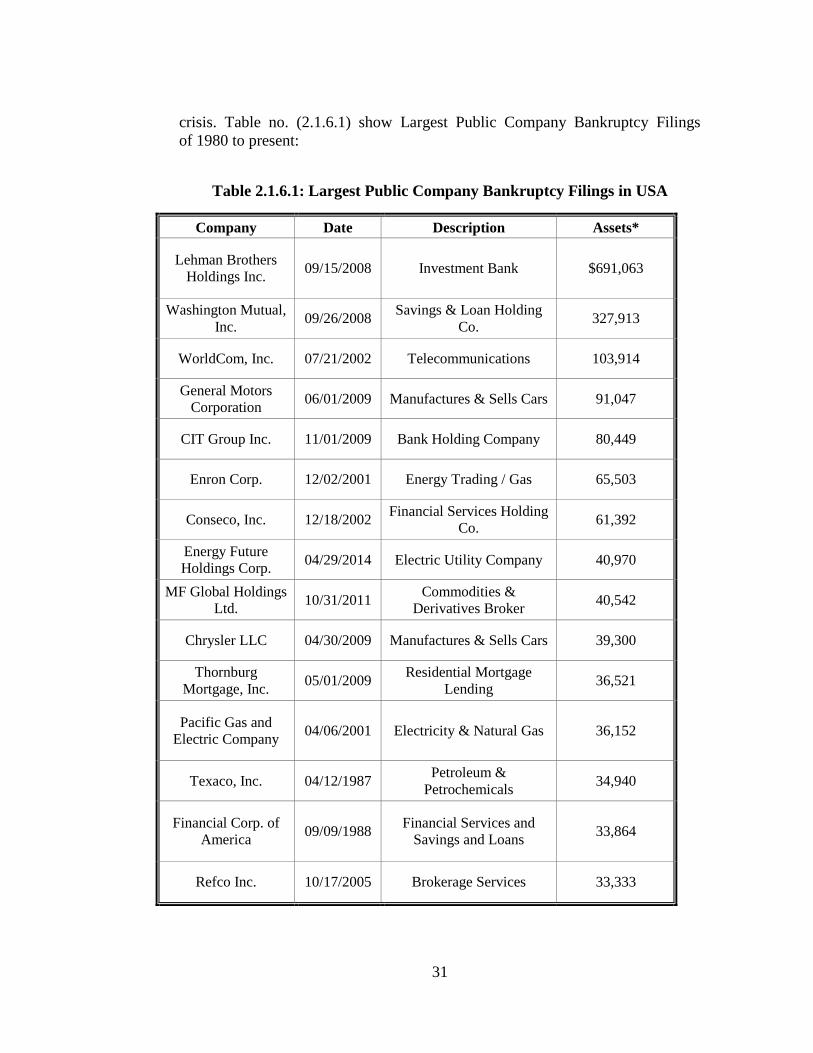
31
crisis. Table no. (2.1.6.1) show Largest Public Company Bankruptcy Filings
of 1980 to present:
Table 2.1.6.1: Largest Public Company Bankruptcy Filings in USA
Company Date Description Assets*
Lehman Brothers
Holdings Inc. 09/15/2008 Investment Bank $691,063
Washington Mutual,
Inc. 09/26/2008
Savings & Loan Holding
Co. 327,913
WorldCom, Inc. 07/21/2002 Telecommunications 103,914
General Motors
Corporation 06/01/2009 Manufactures & Sells Cars 91,047
CIT Group Inc. 11/01/2009 Bank Holding Company 80,449
Enron Corp. 12/02/2001 Energy Trading / Gas 65,503
Conseco, Inc. 12/18/2002 Financial Services Holding
Co. 61,392
Energy Future
Holdings Corp. 04/29/2014 Electric Utility Company 40,970
MF Global Holdings
Ltd. 10/31/2011
Commodities &
Derivatives Broker 40,542
Chrysler LLC 04/30/2009 Manufactures & Sells Cars 39,300
Thornburg
Mortgage, Inc. 05/01/2009
Residential Mortgage
Lending 36,521
Pacific Gas and
Electric Company 04/06/2001 Electricity & Natural Gas 36,152
Texaco, Inc. 04/12/1987 Petroleum &
Petrochemicals 34,940
Financial Corp. of
America 09/09/1988
Financial Services and
Savings and Loans 33,864
Refco Inc. 10/17/2005 Brokerage Services 33,333
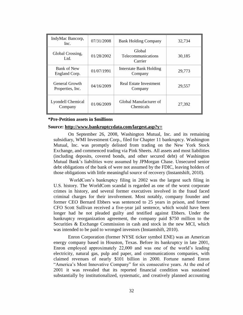
32
IndyMac Bancorp,
Inc. 07/31/2008 Bank Holding Company 32,734
Global Crossing,
Ltd. 01/28/2002
Global
Telecommunications
Carrier
30,185
Bank of New
England Corp. 01/07/1991
Interstate Bank Holding
Company 29,773
General Growth
Properties, Inc. 04/16/2009
Real Estate Investment
Company 29,557
Lyondell Chemical
Company 01/06/2009
Global Manufacturer of
Chemicals 27,392
*Pre-Petition assets in $millions
Source: http://www.bankruptcydata.com/largest.asp?y=
On September 26, 2008, Washington Mutual, Inc. and its remaining
subsidiary, WMI Investment Corp., filed for Chapter 11 bankruptcy. Washington
Mutual, Inc. was promptly delisted from trading on the New York Stock
Exchange, and commenced trading via Pink Sheets. All assets and most liabilities
(including deposits, covered bonds, and other secured debt) of Washington
Mutual Bank‘s liabilities were assumed by JPMorgan Chase. Unsecured senior
debt obligations of the bank of were not assumed by the FDIC, leaving holders of
those obligations with little meaningful source of recovery (Instantshift, 2010).
WorldCom‘s bankruptcy filing in 2002 was the largest such filing in
U.S. history. The WorldCom scandal is regarded as one of the worst corporate
crimes in history, and several former executives involved in the fraud faced
criminal charges for their involvement. Most notably, company founder and
former CEO Bernard Ebbers was sentenced to 25 years in prison, and former
CFO Scott Sullivan received a five-year jail sentence, which would have been
longer had he not pleaded guilty and testified against Ebbers. Under the
bankruptcy reorganization agreement, the company paid $750 million to the
Securities & Exchange Commission in cash and stock in the new MCI, which
was intended to be paid to wronged investors (Instantshift, 2010).
Enron Corporation (former NYSE ticker symbol ENE) was an American
energy company based in Houston, Texas. Before its bankruptcy in late 2001,
Enron employed approximately 22,000 and was one of the world‘s leading
electricity, natural gas, pulp and paper, and communications companies, with
claimed revenues of nearly $101 billion in 2000. Fortune named Enron
―America‘s Most Innovative Company‖ for six consecutive years. At the end of
2001 it was revealed that its reported financial condition was sustained
substantially by institutionalized, systematic, and creatively planned accounting
33
fraud, known as the ―Enron scandal‖. The Enron scandal, revealed in October
2001, eventually led to the bankruptcy of the Enron Corporation, the dissolution
of Arthur Andersen, which was one of the five largest audit and accountancy
partnerships in the world. In addition to being the largest bankruptcy
reorganization in American history at that time, Enron undoubtedly is the biggest
audit failure (Instantshift, 2010).
Thornburg Mortgage Inc. was an American publicly traded corporation
headquartered in Santa Fe, New Mexico. Founded in 1993, the company is a real
estate investment trust (REIT) that originates, acquires & manages mortgages,
with a specific focus on jumbo and super jumbo adjustable rate mortgages.
During the Financial crisis of 2007–2010 the company experienced financial
difficulties related to the ongoing subprime mortgage crisis, and on April 1, 2009
Thornburg Mortgage, Inc. and four of its affiliates (collectively, the ―Debtors‖)
filed petitions in the United States Bankruptcy Court for the District of Maryland
seeking relief under chapter 11 of the United States Bankruptcy Code. After the
sale of all remaining assets, it would no longer exist as a going concern.
(Instantshift, 2010).
From previous cases the researcher can say there are many factors that
lead to business failure such as external factors (general economic condition) like
global economic crisis that leads to bankrupt many large firms such as Lehman
Brothers, Washington Mutual, Chrysler, and General Motors all filed for
bankruptcy protection, or internal factors (company-specific factors) such as
management causes like fraud that leads to bankrupt many large firms such as
Enron and WorldCom.
Bankrupt very large firms or sectors might cause the entire financial
system to collapse and eventually harm the economy, for example, the failure of
Lehman Brothers in September 2008 contributed to increase the global recession.
Government can intervene to reduce failure to protect large firms and thereby
protect the economy of the country, like ―the government helped arrange the
2008 acquisition of Wachovia by Wells Fargo, the 2008 acquisition of Bear
Sterns by JPMorgan Chase, and the 2009 acquisition of Merrill Lynch by Bank
of America‖ (Ehrhardt & Brigham, 2011, p. 870).
In 2008 and 2009 the government provided billions of dollars of
financing to General Motors and Chrysler. Even though these companies
subsequently went through bankruptcy proceedings in 2009, they avoided
liquidation, still have a significant number of employees, and remain major
players in the automobile industry. In past years, the government also has
intervened to support troubled firms in other critical sectors, such as Lockheed
and Douglas Aircraft in the defense industry (Ehrhardt & Brigham, 2011, p.
871).
34
2.1.7 Resolving Financial Distress
There are many ways to deal with bankruptcy problem either informal
(private) or formal (court-supervised) resolutions of financial distress.
First the researcher will discuss the methods of resolution of financial
distress outside the bankruptcy court system then the researcher will discussed in
briefly methods of formal resolution (court-supervised) in USA.
2.1.7.1 Informal Methods of Resolving Financial Distress
There are many methods to deal with bankruptcy problem outside the
court system which include:
A. Debt restructuring.
B. Asset sales.
C. Financing from outside sources.
A. Debt Restructuring.
In the case of an economically sound company whose financial
difficulties appear to be temporary, creditors are generally willing to work
with the company to help it recover and reestablish itself on a sound
financial basis. Such voluntary plans, commonly called workouts, usually
require a restructuring of the firm‘s debt, because current cash flows are
insufficient to service the existing debt (Ehrhardt & Brigham, 2011, p.
872).
Publicly-held debt contracts and privately-held ones are usually subject to
different disclosure and regulatory constraints. The restructuring of public
debt is governed primarily by the Trust Indenture Act of 1939. This Act
requires unanimous consent by the holders of a particular class of debt
securities in order to change the debt obligation‘s maturity, principal, or
coupon rate. These stringent voting rules effectively preclude a private
restructuring of public corporate debt. As a result, virtually all informal
public debt restructurings are accomplished through a tender offer in
which debt is repurchased with cash, or by an exchange offer in which
existing debt is exchanged for new securities including debt, equity, or a
combination of both. The restructuring also often includes covenant
modifications (Senbet & Wang, 2010, p. 253).
The advantages of informal reorganization are less costly, relatively
simple to create and typically allows creditors to recover more money and
sooner.
35
B. Sales of Assets
An alternative method to handle financial distress is sale of assets which
consider a quick way to collect cash and create liquidity in short period.
A partial sell-off of the firm‘s existing assets generates cash that can be
used to reduce outstanding debt or to undertake new investment
opportunities. The price received by the seller in an asset sale is
ultimately determined by the outcome of a bargaining process between
the buyer and the seller. The poor financial condition and the urgent
liquidity need of the distressed seller can severely weaken the firm‘s
bargaining position, and therefore reduce the price it receives for the
assets. Furthermore, if the sale is conducted under duress from the firm‘s
creditors, the outcome may be that the price received is less than the value
of the asset under current management by the distressed firm (Senbet &
Wang, 2010, p. 254).
C. Financing From Outside Sources.
Also attracting funds from outside will help the distressed firm to survive.
The distressed firm needs sufficient cash to pay employees, suppliers, and
other stakeholders. The distressed firm may also have positive net present
value projects available that need to be financed. Thus, the firm‘s ability
to attract new capital is crucial for the firm‘s survival and investment
efficiency (Senbet & Wang, 2010, p. 254).
2.1.7.2 Federal Bankruptcy Law3
U.S. bankruptcy laws were first enacted in 1898. They were modified
substantially in 1938 and again in 1978, and some fine-tuning was done
in 1986. In 2005, Congress further modified the bankruptcy code,
speeding up bankruptcy proceedings for companies and making it more
difficult for consumers to take advantage of provisions that can wipe out
certain debts. The primary purpose of the bankruptcy law is to avoid
firms that are worth more as ongoing concerns being put out of business
by individual creditors, who could force liquidation without regard to the
effects on other parties (Ehrhardt & Brigham, 2011, p. 874).
Chapters 1, 3, and 5 contain general provisions applicable to the other
chapters. Chapter 11, which deals with business reorganization, is the
most important section from a financial management viewpoint. Chapter
7 details the procedures to be followed when liquidating a firm; generally,
3 To read more about Bankruptcy Law, see Altman, E. (1993). In Corporate Financial Distress
and Bankruptcy (2 Ed.). New York, NY: John Wiley & Sons, Inc.
36
Chapter 7 does not come into play unless it has been determined that
reorganization under Chapter 11 is not feasible. Chapter 9 deals with
financially distressed municipalities; Chapter 12 covers special
procedures for family-owned farms; Chapter 13 covers the adjustment of
debts for ―individuals with regular income‖; and Chapter 15 sets up a
system of trustees who help administer proceedings under the act
(Ehrhardt & Brigham, 2011, pp. 874-875).
The researcher focused in briefly on chapter 11 which deals with business
reorganization and chapter7 that details the procedures to be followed
when liquidating a firm which are related to the topic of the study.
2.1.7.3 There are Two Types of Court- Formal (Court-Supervised) Methods
of Resolving Financial Distress
Supervised methods to resolve bankruptcy either voluntary bankruptcy or
involuntary bankruptcy. Voluntary bankruptcy, a bankruptcy petition
filed in federal court by the distressed firm‘s management. Involuntary
bankruptcy, a bankruptcy petition filed in federal court by the distressed
firm‘s creditors. There are many advantages for formal bankruptcy
include: avoids holdout problems, due to automatic stay provision avoids
common pool problem, Interest and principal payments may be delayed
without penalty until reorganization plan is approved, gives debtor
exclusive right to submit a proposed reorganization plan for agreement
from the parties involved, reduces fraudulent conveyance problem
(Ehrhardt & Brigham, 2011).
2.1.8 Liquidation in Bankruptcy
In law and business, liquidation is the process by which a company (or
part of a company) is brought to an end, and the assets and property of the
company are redistributed. Liquidation is also sometimes referred to as winding-
up or dissolution, although dissolution technically refers to the last stage of
liquidation. The process of liquidation also arises when customs, an authority or
agency in a country responsible for collecting and safeguarding customs duties,
determines the final computation or ascertainment of the duties or drawback
accruing on an entry (Wikipedia, 2015).
Liquidation may either be compulsory (sometimes referred to as a
creditors' liquidation) or voluntary (sometimes referred to as a shareholders'
liquidation, although some voluntary liquidations are controlled by the creditors
(Wikipedia, 2015).
If a company is ―too far gone‖ to be reorganized, then it must be
liquidated. Liquidation should occur when the business is worth more dead than
alive, or when the possibility of restoring it to financial health is remote and the
37
creditors are exposed to a high risk of greater loss if operations are continued
(Ehrhardt & Brigham, 2011, p. 885).
Liquidation in bankruptcy is executed by the jurisdiction of a federal
bankruptcy court. Chapter 7 of the Federal Bankruptcy Reform Act of 1978 deals
with liquidation and there is list of priority of claims in chapter 7 of liquidation
(Ehrhardt & Brigham, 2011):
Secured creditors.
Trustee‘s administrative costs.
Expenses incurred after involuntary case begun but before trustee appointed.
Wages due workers within 3 months prior to filing.
Unpaid contributions to employee benefit plans that should have been paid
within 6 months prior to filing.
Unsecured claims for customer deposits.
Taxes due.
Unfunded pension plan liabilities.
General (unsecured) creditors.
Preferred stockholders.
Common stockholders.
2.1.9 Failure Prediction Models
Some of the earliest research on the topic of using financial ratios to
predict financial failure was performed by Beaver (1966) using a univariate
analysis method.
The researchers from the past in the sixties began to use financial ratios to
predict failure by using various predicting models; the researcher will discuss
William Beaver model and Altman‘s models in briefly.
2.1.9.1 Models for Predicting Bankruptcy
One of the important items in decision making of investors is predicting
bankruptcy. Thus, in recent years Academic research community is trying
to make exact models for this purpose, including:
The William Beaver 1966.
Altman models 1968.
Kane models in 1972.
Aspryngt models in 1978.
Ahlsvn models in 1980.
Toffler models in 1983.
Zmyjvsky models in 1984.
Falmr models in 1984.
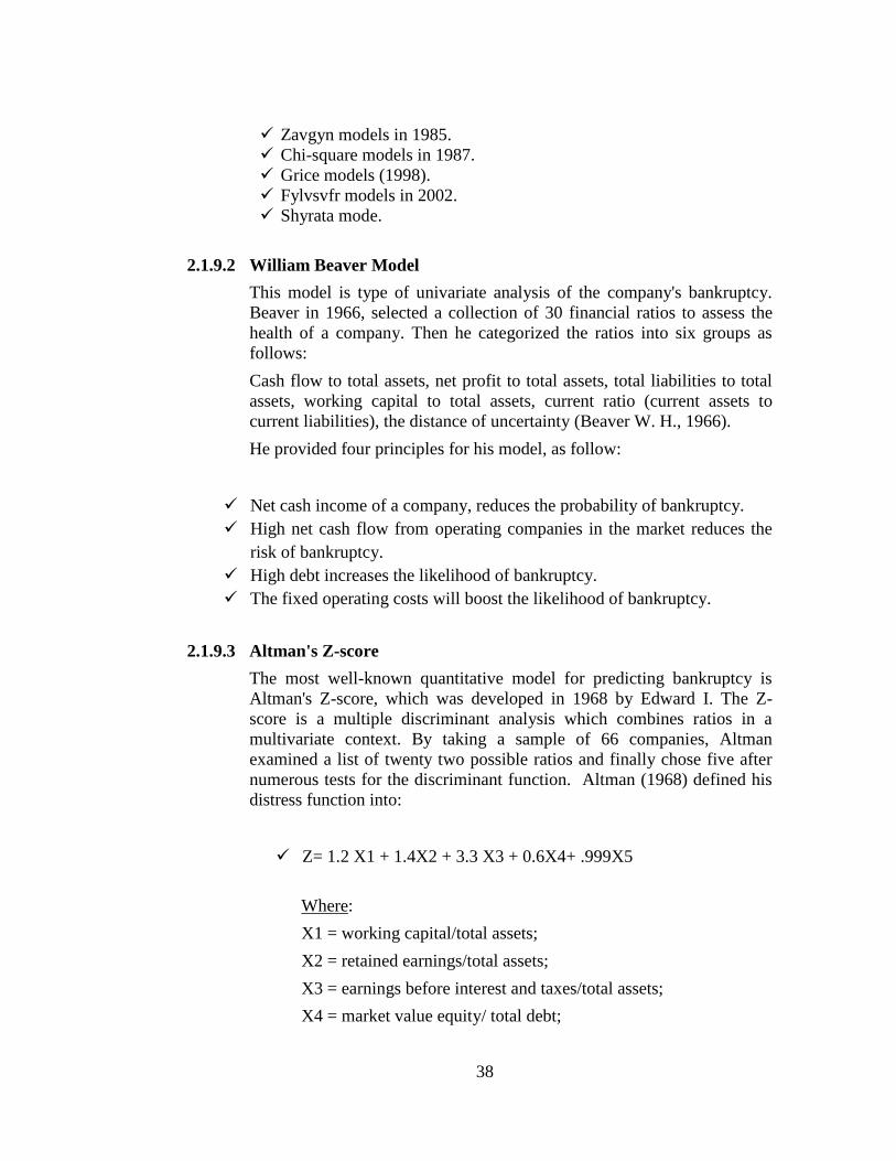
38
Zavgyn models in 1985.
Chi-square models in 1987.
Grice models (1998).
Fylvsvfr models in 2002.
Shyrata mode.
2.1.9.2 William Beaver Model
This model is type of univariate analysis of the company's bankruptcy.
Beaver in 1966, selected a collection of 30 financial ratios to assess the
health of a company. Then he categorized the ratios into six groups as
follows:
Cash flow to total assets, net profit to total assets, total liabilities to total
assets, working capital to total assets, current ratio (current assets to
current liabilities), the distance of uncertainty (Beaver W. H., 1966).
He provided four principles for his model, as follow:
Net cash income of a company, reduces the probability of bankruptcy.
High net cash flow from operating companies in the market reduces the
risk of bankruptcy.
High debt increases the likelihood of bankruptcy.
The fixed operating costs will boost the likelihood of bankruptcy.
2.1.9.3 Altman's Z-score
The most well-known quantitative model for predicting bankruptcy is
Altman's Z-score, which was developed in 1968 by Edward I. The Z-
score is a multiple discriminant analysis which combines ratios in a
multivariate context. By taking a sample of 66 companies, Altman
examined a list of twenty two possible ratios and finally chose five after
numerous tests for the discriminant function. Altman (1968) defined his
distress function into:
Z= 1.2 X1 + 1.4X2 + 3.3 X3 + 0.6X4+ .999X5
Where:
X1 = working capital/total assets;
X2 = retained earnings/total assets;
X3 = earnings before interest and taxes/total assets;
X4 = market value equity/ total debt;
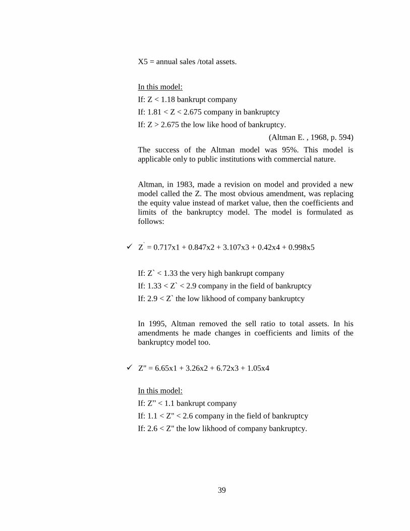
39
X5 = annual sales /total assets.
In this model:
If: Z < 1.18 bankrupt company
If: 1.81 < Z < 2.675 company in bankruptcy
If: Z > 2.675 the low like hood of bankruptcy.
(Altman E. , 1968, p. 594)
The success of the Altman model was 95%. This model is
applicable only to public institutions with commercial nature.
Altman, in 1983, made a revision on model and provided a new
model called the Z. The most obvious amendment, was replacing
the equity value instead of market value, then the coefficients and
limits of the bankruptcy model. The model is formulated as
follows:
Z` = 0.717x1 + 0.847x2 + 3.107x3 + 0.42x4 + 0.998x5
If: Z` < 1.33 the very high bankrupt company
If: 1.33 < Z` < 2.9 company in the field of bankruptcy
If: 2.9 < Z` the low likhood of company bankruptcy
In 1995, Altman removed the sell ratio to total assets. In his
amendments he made changes in coefficients and limits of the
bankruptcy model too.
Z" = 6.65x1 + 3.26x2 + 6.72x3 + 1.05x4
In this model:
If: Z‖ < 1.1 bankrupt company
If: 1.1 < Z" < 2.6 company in the field of bankruptcy
If: 2.6 < Z" the low likhood of company bankruptcy.
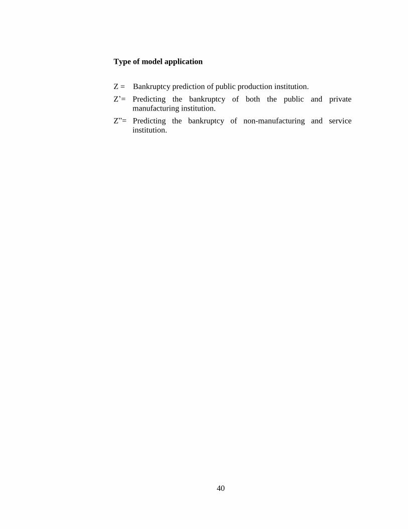
40
Type of model application
Z = Bankruptcy prediction of public production institution.
Z‘= Predicting the bankruptcy of both the public and private
manufacturing institution.
Z‖= Predicting the bankruptcy of non-manufacturing and service
institution.
41
2.2 Using Financial Analysis and Financial Ratios to Predict
Failure
Section two highlights the cash flow statement and presents accounting
conventions, financial analysis and types of financial analysis. Also, this section
talks about financial ratios, types of financial ratios, the limitations of financial
ratios and finally using of accounting ratios to predict financial failure.
2.2.1 The Statement of Cash Flow
A statement reporting the impact of a firm‘s operating, investing and
financing activities on cash flows over an accounting period (Brigham &
Houston, 2004, p. 50).
The statement separates activities into three categories:
A. Operating activities, which includes net income, depreciation, and
changes in current assets and current liabilities other than cash and
short-term debt.
B. Investing activities, which include investments in or sales of fixed assets.
C. Financing activities, which includes cash raised during the year by
issuing short-term debt, long-term debt, or stock. Also, since dividends
paid or cash used to buy back outstanding stock or bonds reduces the
company‘s cash, such transactions are included here.
Financial failure of many projects results of the lack of the capital that
results from ignoring to assess of prepared financial facility needs. The cash flow
statement is not the solution as soon as you prepare it you will solve the
problems, but it is the report that gives the management a picture of the financial
problems of the plant expected to face the facility in the near future. The cash
flow planning in the facility one of the most important elements of success of
fiscal policy, the lack of a financial planning will make the facility to face one of
two things:
The facility may find itself facing cash outflows more than the cash
inflows.
The facility face increase in the cash inflows more than the cash outflows
and thus there will be money idle without any use.
42
The preparation of statement of cash flows require to predicts all the
processes that affect the volume of cash and put detailed estimates of the
amount and timing of cash inflows and outflows resulting from the
exercise of any activity within the facility and thus the facility determine
all of its operations and identify processes affecting cash flow.
2.2.2 The Objectives of The Cash Flow Statement
There are many objectives of CFS as follow:
A. Cash flow planning helps management to keep the least amount of
liquidity to meet the current obligations of the facility and use the largest
amount of cash in the assets of the facility for profits.
B. Helps to determine the size of the surplus thus enabling the facility to
direct their investments more appropriate in terms of return and in light of
the magnitude and timing of the extra money.
C. Cash flows planning help to know the size and time of deficit or surplus
cash.
D. Assist in developing policies to face the debts in a timely manner.
E. Enables the list of cash flows to achieve control over cash flows in the
enterprise.
F. The statement of cash flows without the other statements is not sufficient
to provide the necessary information to employees and other creditors.
2.2.3 Steps to Prepare The Cash Flow Statement
To prepare the statement of cash flows you need to follow these steps:
A. Estimate the cash inflows (receipts)
B. Estimated cash outflows (payments)
C. Compared inflows (receipts) to outflows (payments).
D. Estimate the minimum level of due cash
Firms in financial distress, generally display dramatically different cash
flow patterns. Firms in reorganization will generally have a negative cash flow
from operations, a positive cash flow from investing activities and a negative
cash flow from financing. The positive inflow from investing is usually due to
the liquidation of excess assets and negative cash flows from financing as they
work to satisfy stakeholders. Distressed firms will also report negative cash flows
from operations and investing, but will still be in the process of raising capital
43
and reporting a positive cash flow from investing activities. These may be the
most dangerous (Danilov, 2014, p. 28).
2.2.4 Definitions and Conventions of Accounting (McLaney, 2009, pp. 46-48)
Accounting is a language that is used to store and communicate economic
information about organizations. It has a set of rules. It is particularly important
that anyone trying to read accounting statements and draw conclusions from
them is clear on the rules of accounting. Severe misunderstandings could arise
for someone not familiar with the rules.
2.2.4.1 Going concern convention
In the absence of evidence to the contrary, it is assumed that the business
will continue indefinitely. This means, for example, that it will be
assumed that a non-current asset will be capable of being used by the
business for the whole of its useful life, rather than it being assumed that
the business will be forced to dispose of the asset as a result of the
business suffering financial collapse. Thus a business can base its
depreciation policy on the cost, expected life and disposal proceeds of the
particular asset, rather than on the current value of the asset at
intermediate points of its life. As a result, the fact that many non-current
assets have a current market value below their balance sheet value does
not cause the prudence convention to be invoked.
2.2.4.2 Accruals basis
Profit or loss is concerned with net increases or decreases in wealth, not
with increases or decreases in cash. Thus when deriving the amount of the
expenses that are to be matched to particular revenues, the fact that cash
may not yet have been paid is not relevant. For example, the cost of
inventories sold, for inclusion in the income statement, will be the same,
irrespective of whether or not payment for the inventories concerned has
yet been made.
2.2.5 Quarterly Vs. Audited Financial Statement
Most traditional analysis relies on annual financial statements primarily
because they have been audited and are therefore are believed to be more reliable
than unaudited, quarterly financial statements. Baldwin and Glezen (1992) found
that there was no statistical evidence to suggest that quarterly financial
statements were less accurate than annual financial statements with regards to
assessing solvency and went on further to suggest that quarterly statements
provided more timely evidence of insolvency than annually issued statements
without a substantial loss of accuracy (Danilov, 2014, p. 29).
44
2.2.6 Techniques of Financial Statement Analysis (Paramasivan &
Subramanian, 2008, p. 14)
Financial statement analysis is interpreted mainly to determine the
financial and operational performance of the business concern. A number of
methods or techniques are used to analyze the financial statement of the business
concern. The following are the common methods or techniques, which are widely
used by the business concern.
A. Comparative Statement Analysis:
Comparative Income Statement Analysis.
Comparative Position Statement Analysis.
B. Trend Analysis.
C. Common Size Analysis.
D. Fund Flow Statement.
E. Cash Flow Statement.
F. Ratio Analysis.
The researcher will discuss the important method of analysis which will
be used in this study to predict business failure which is ratios analysis then the
researcher will mention the types of financial ratios and finally limitations of the
financial ratios.
2.2.7 Ratios Analysis
2.2.7.1 Ratio Analysis Definitions
Financial statements report both on a firm‘s position at a point in time and
on its operations over some past period. However, the real value of
financial statements lies in the fact that they can be used to help predict
future earnings and dividends. From an investor‘s standpoint, predicting
the future is what financial statement analysis is all about, while from
management‘s standpoint, financial statement analysis is useful both to
help anticipate future conditions and, more important, as a starting point
for planning actions that will improve the firm’s future performance.
Financial ratios are designed to help one evaluate a financial statement
(Brigham & Houston, 2004, p. 97).
Ratio analysis involves methods of calculating and interpreting financial
45
ratios to analyze and monitor the firm‘s performance. The basic inputs to
ratio analysis are the firm‘s income statement and balance sheet (Gitman,
2002, p. 49).
Ratio analysis is a commonly used tool of financial statement analysis.
Ratio is a mathematical relationship between one number to another
number. Ratio is used as an index for evaluating the financial
performance of the business concern. An accounting ratio shows the
mathematical relationship between two figures, which have meaningful
relation with each other (Paramasivan & Subramanian, 2008, pp. 20-21).
Financial ratios are designed to extract important information that might
not be obvious simply from examining a firm‘s financial statements
(Ehrhardt & Brigham, 2011, p. 89).
From previous definitions we can say ratio analysis is a tool of financial
statement analysis which is a mathematical relationship between two
figures that used to analyze, monitor and evaluate financial performance
of the firm.
2.2.7.2 Interested Parties
There are many parties involved in financial analysis and every group
seek to answer a series of questions that affect their interests by analyzing
financial statements and explain its results. These parties are:
A. Present and potential investors.
B. Lenders.
C. Customers and suppliers.
D. Governmental institutions.
A. Present and potential investors
Investors are more interested in the return on equity because they want to
insure the effectiveness of their investments, so they are looking which
better to keep their investments or to give up.
Both present and prospective shareholders are interested in the firm‘s
current and future level of risk and return, which directly affect share
price (Gitman, 2002, p. 49).
B. Lenders
Banks and creditors are more interested in the debt ratios to insure the
project ability to settle its loan. They interested primarily in the short term
46
liquidity of the company and its ability to make interest and principal
payments.
A second concern of creditors is the firm's profitability, they want
assurance that the business is healthy (Gitman, 2002, p. 49).
C. Management
Like stockholders, is concern with all aspects of the firm's financial
situation, and its attempts to produce financial ratios that will be
considered favourable by both owners and creditors. In addition,
management uses ratios to monitor the firm's performance (Gitman, 2002,
p. 49).
2.2.7.3 Categories of Financial Ratios
Financial ratios can be divided for convenience into five basic categories:
liquidity, activity, debt, profitability, market ratios. Liquidity, activity,
and debt ratios primarily measure risk. Profitability ratios measure return.
Market ratios capture both risk and return (Gitman, 2002, p. 53). These
categories beside cash flow ratios will be discussed in briefly. The basic
categories of financial ratios is as follow:
A. Liquidity (Solvency) Ratios.
B. Activity Ratios.
C. Leverage Ratios .
D. Profitability Ratios
E. Market Ratios.
A. Liquidity Ratios
The liquidity of a firm is measured by its ability to satisfy its short-term
obligations as they come due. Liquidity refers to the solvency of the
firm‘s overall financial position—the ease with which it can pay its bills.
Because a common precursor to financial distress and bankruptcy is low
or declining liquidity, these ratios are viewed as good leading indicators
of cash flow problems. The two basic measures of liquidity are the
current ratio and the quick (acid-test) ratio (Gitman, 2002, p. 54).
47
B. Activity Ratios
Activity ratios measure the speed with which various accounts are
converted into sales or cash—inflows or outflows. With regard to current
accounts, measures of liquidity are generally inadequate because
differences in the composition of a firm‘s current assets and current
liabilities can significantly affect its ―true‖ liquidity. It is therefore
important to look beyond measures of overall liquidity and to assess the
activity (liquidity) of specific current accounts. A number of ratios are
available for measuring the activity of the most important current
accounts, which include inventory, accounts receivable, and accounts
payable. The efficiency with which total assets are used can also be
assessed (Gitman, 2002, p. 55).
C. Debt Management Ratios
The extent to which a firm uses debt financing, or financial leverage, has
three important implications: (1) By raising funds through debt,
stockholders can maintain control of a firm without increasing their
investment. (2) If the firm earns more on investments financed with
borrowed funds than it pays in interest, then its shareholders‘ returns are
magnified, or ―leveraged,‖ but their risks are also magnified. (3) Creditors
look to the equity, or owner-supplied funds, to provide a margin of safety
so the higher the proportion of funding supplied by stockholders, the less
risk creditors face. (Ehrhardt & Brigham, 2011, p. 95).
It is also called as leverage ratio, which measures the long-term obligation
of the business concern. This ratio helps to understand, how the long-term
funds are used in the business concern (Paramasivan & Subramanian,
2008, p. 22).
D. Profitability Ratio
Profitability is the net result of a number of policies and decisions. The
ratios examined thus far provide useful clues as to the effectiveness of a
firm‘s operations, but the profitability ratios go on to show the combined
effects of liquidity, asset management, and debt on operating results
(Brigham & Houston, 2004, p. 98).
There are many measures of profitability. As a group, these measures
enable the analyst to evaluate the firm‘s profits with respect to a given
level of sales, a certain level of assets, or the owners‘ investment. Without
profits, a firm could not attract outside capital. Owners, creditors, and
management pay close attention to boosting profits because of the great
importance placed on earnings in the marketplace (Gitman, 2002, p. 61).
48
E. Market Value Ratios
A final group of ratios, the market value ratios, relates the firm‘s stock
price to its earnings, cash flow, and book value per share. These ratios
give management an indication of what investors think of the company‘s
past performance and future prospects. If the liquidity, asset management,
debt management, ratios all look good, then the market value ratios will
be high, and the stock price will probably be as high as can be expected
(Brigham & Houston, 2004, p. 102).
2.2.7.4 Cash Flow Ratios (About Money, 2015)
Under generally accepted accounting principles, a company can easily
report a large income figure, even while its cash reserves are draining
away. The cash flow from operations ratio can be used to determine the
extent to which cash flow differs from the reported level of either
operating income or net income. Any difference in the ratio that varies
significantly from one is indicative of substantial noncash expenses or
sales in the reported income figures. Cash flow problems are likely if the
ratio is substantially less than one (Bragg, 2002, p. 49).
Cash flow analysis uses ratios that focuses on cash flow and how solvent,
liquid, and viable the company is. Here are the most important cash flow
ratios:
A. Operating Cash Flow Ratio
The operating cash flow ratio is one of the most important cash flow
ratios. Cash flow is an indication of how money moves into and out of
the company and how you pay your bills. Operating cash flow relates
to cash flows that a company accrues from operations to its current
debt. It measures how liquidity a firm is in the short run since it relates
to current debt and cash flows from operations. Operating Cash Flows
Ratio = Cash Flows From Operations/Current Liabilities where: Cash
Flows from Operations comes off the Statement of Cash Flows and
Current Liabilities comes off the Balance Sheet. If the Operating Cash
Flow Ratio for a company is less than 1.0, the company is not
generating enough cash to pay off its short-term debt which is a serious
situation. It is possible that the firm may not be able to continue to
operate.
49
B. Price/Cash Flow Ratio
The price to cash flow ratio is often considered a better indication of a
company's value than the price to earnings ratio. It is a really useful
ratio for a company to know, particularly if the company is publicly
traded. It compares the company's share price to the cash flow the
company generates on a per share basis. Calculate the price/cash flow
ratio as follows: Price/cash flow ratio = Share price/Operating cash
flow per share where: Share price is usually the closing price of the
stock on a particular day and operating cash flow is taken from
the Statement of Cash Flows. Some business owners use free cash
flow in the denominator instead of operating cash flow. It should be
noted that most analysts still use price/earnings ratio
in valuation analysis.
C. Cash Flow Margin Ratio
The Cash Flow Margin ratio is an important ratio as it expresses the
relationship between cash generated from operations and sales. The
company needs cash to pay dividends, suppliers, service debt, and
invest in new capital assets, so cash is just as important as profit to a
business firm. The Cash Flow Margin ratio measures the ability of a
firm to translate sales into cash. The calculation is: Cash flow from
operating cash flows/Net sales. The numerator of the equation comes
from the firm's Statement of Cash Flows. The denominator comes
from the Income Statement. The larger the percentage, the better.
D. Cash Flow from Operations/Average Total Liabilities
Cash flow from Operations/Average total liabilities is a similar ratio to
the commonly-used total debt/total assets ratio. Both measure the
solvency of a company or its ability to pay its debts and keep its head
above water. The former is better, however, as it measures this ability
over a period of time rather than at a point in time. This ratio is
calculated as follows: Cash flow from Operations/Average Total
Liabilities, where: cash flow from operations is taken from
the Statement of Cash Flows and average total liabilities is an average
of total liabilities from several time periods of liabilities taken from
balance sheets. The higher the ratio, the better the firm's financial
flexibility and its ability to pay its debts.
50
2.2.7.5 Limitations of Ratio Analysis (Ehrhardt & Brigham, 2011, p. 109)
A. Many large firms operate different divisions in different industries, and
for such companies it is difficult to develop a meaningful set of industry
averages. Therefore, industry averages are more applicable to small,
narrowly focused firms than to large, multidivisional ones.
B. To set goals for high-level performance, it is best to benchmark on the
industry leaders‘ ratios rather than the industry average ratios.
C. Inflation may have badly distorted firms‘ balance sheets—reported values
are often substantially different from ―true‖ values. Further, because
inflation affects depreciation charges and inventory costs, reported profits
are also affected. Thus, inflation can distort a ratio analysis for one firm
over time or a comparative analysis of firms of different ages.
D. Seasonal factors can also distort a ratio analysis. For example, the
inventory turnover ratio for a food processor will be radically different if
the balance sheet figure used for inventory is the one just before versus
the one just after the close of the canning season. This problem can be
minimized by using monthly averages for inventory (and receivables)
when calculating turnover ratios.
E. Firms can employ ―window dressing‖ techniques to make their financial
statements look stronger.
F. Different accounting practices can distort comparisons.
2.2.7.6 Cautions About Using Ratio Analysis (Gitman, 2002, p. 53)
A. Ratios with large deviations from the norm only indicate symptoms of a
problem. Additional analysis is typically needed to isolate the causes of
the problem. The fundamental point is this: Ratio analysis merely directs
attention to potential areas of concern; it does not provide conclusive
evidence as to the existence of a problem.
B. A single ratio does not generally provide sufficient information from
which to judge the overall performance of the firm. Only when a group of
ratios is used can reasonable judgments be made. However, if an analysis
is concerned only with certain specific aspects of a firm‘s financial
position, one or two ratios may be sufficient.
51
C. It is preferable to use audited financial statements for ratio analysis. If
have not been audited, the data contained in them may not reflect the
firm‘s true financial condition.
2.2.7.7 Using Accounting Ratios to Predict Financial Failure (McLaney,
2009, p. 66)
One objective of ratio analysis is to try to make a judgment about a
particular business‘s ability to survive and to prosper. Originally, interest
focused on identifying individual ratios that might represent good
indicators of likely financial collapse. Researchers, therefore, sought to be
able to make statements such as: if the value for a particular ratio (such as
the acid test ratio) fell below a particular threshold figure, the business
was then significantly at risk. They attempted to do this by identifying
particular ratios that might be good discriminators between potential
failures and survivors. The researchers then found a group of businesses
that had actually collapsed. They matched this with a second group of
non-failed businesses, one of which was as like one of the collapsed
group as possible in size, industry and so forth. This provided them with
two groups, as far as possible identical, except that all the members of
one group had collapsed and none of the second group had. Using past
data on all the businesses, attempts were made to examine whether the
particular ratios selected were significantly different between the two
groups during the period (say, five years) leading up to the date of the
collapse of the failed businesses. Where there were significant differences
for a specific ratio, it was possible to say that a figure of above a
particular level implied that the business was safe, whereas a figure below
this benchmark implied that it was at risk. Although researchers achieved
some success at identifying ratios that were reasonably good
discriminators, thoughts turned to the possibility that combining several
quite good discriminator ratios might produce a Z-score (so called) that
would be a very good discriminator.
52
2.3 Overview of Palestine Securities Exchange
This section briefly talks about the emergence and development of the
Palestine securities exchange, the objectives of the PEX, the listed companies in
the PEX and finally this section presents the cases in which the listed companies
will be delisted.
2.3.1 The Emergence and The Development of The Palestine Securities
Exchange (Palestine Exchange, 2015)
Founded in 1995, and holding its first trading session in February 1997,
the PEX began as the first private sector-owned stock exchange in the Arab
world. In 2010, it converted into a public shareholding company with paid-up
capital of US $10 million. This transformation was accompanied by a new
corporate identity bearing the brand name ―Palestine Exchange‖ and the slogan
―Palestine of Opportunities.‖ Committed to the principles of good governance,
the PEX listed for trading on April 4, 2012 thus becoming the second Arab
exchange to do so. The PEX is registered with the Companies Controller at the
Ministry of National Economy under registration number (562601187).
The PEX focuses on attracting regional and international individual and
institutional investors, including Palestinian diaspora. Currently, the PEX
conducts its business through its head – quarters in Nablus and its representative
office in Ramallah. Since its inception as the first fully automated Arab
exchange, the PEX has sought to mesh the latest financial market technology
with best practice governance and management to ensure maximum
transparency, integrity and investor protection.
Along with securities trading, the PEX offers transaction processing
services through its Clearing Depository Settlement Center (CDS). These include
opening investor accounts, off-floor transactions, issuing share books and
ownership certificates. Monitored by the SMARTS market surveillance platform,
the HORIZON system carries out trading transactions. Settlement and clearing
transactions are carried out through the Clearing Depository & Settlement Center
(CDS) electronic system linked to the trading system. During the settlement
process, securities are transferred from the seller to the buyer in T+3, while
clearing is done through the settlement bank (Arab Bank). HSBC bank acts as a
custodian for securities on behalf of foreign investors.
On 31 December 2012, 48 companies with a total market value of some
US$2.86 billion were listed on the PEX. They encompassed five economic
sectors: banking and financial services, insurance, investment, industry, and
services. Shares trade in Jordanian dinars and US dollars. Only ordinary shares
trade but there remains the possibility and readiness for trading other securities in
the future. On 31 December 2012, nine member securities companies (brokerage
53
firms) distributed among different cities in the West Bank and Gaza Strip
operated in the PEX.
The PEX maintain a regional and international presence through
membership in several specialized federations:
Federation of Arab Stock Exchanges.
Federation of Euro-Asian Stock Exchanges (FEAS).
World Federation of Exchanges – WFE (Affiliate Member).
Forum of Islamic Stock Exchanges.
Africa & Middle East Depositories Association (AMEDA).
Association of National Numbering Agencies (ANNA).
2.3.2 The Objectives of Palestine Securities Exchange
Palestine Stock Exchange is trying to achieve many goals, the most
important is as follow: (Palestine Exchange, 2015):
To provide a safe trading environment that serves investors and protects
their interests.
To increase the investment awareness of the local community and
enhance PEX relation with local, regional and international financial
institutions and Associations.
To develop domestic investments and attract Palestinian Diaspora &
foreign capital.
To increase market depth and provide new and diverse financial tools and
services.
To create a proficient working environment within the PEX by investing
in human capital and maintaining state of the art technologies of stock
markets.
2.3.3 The Listed Companies in PEX
The PEX encompassed five economic sectors: banking and financial
services, insurance, investment, industry, and services sectors. The economic
sectors and the listed companies for each sector in the PEX at the end of 2014
are shown in appendix no. (2).
54
2.3.4 Delisting Companies
Following Palestinian capital market authority approval, PEX may delist listed
companies shares in the following events (Palestine Exchange, 2015):
A. If it appears that material information was stated in the listing application
or any material documents supplied were incorrect, forged, misleading, or
missing or the Company failed to submit required documents to the PEX
upon request.
B. If the number of shareholders decreased below 50 shareholders for
companies listed in the Second Market for a period of 3 consecutive
months during one year.
C. If it appears from the audit report that the company is unable to meet its
debt obligations, or unable to finance its activities, or its net shareholders
equity to the paid capital is less than 20%.
D. If the listed company ceases to exist as a corporate entity because of a
merger with other company (ies) or because of liquidation.
E. If the company shares or bonds were not traded for an entire one year, or
the listing was suspended for over a year without adjusting the company
its status pursuant to the Securities Trading Rule as issued by the PEX.
F. If the company violates any of its obligations as stipulated in the listing
agreement or Law or PEX rules.
G. In all other events that infringe the protected rights of the investors or to
serve public interest.
H. If the listing of the foreign company shares where they were originally
listed in a foreign exchange was delisted.
I. If the foreign company no longer has a branch in Palestine or legal
representative for more than one month.
55
2.4 Multiple Linear Discriminant VS. Logistic Regression
Model
Section four presents the statistical models for predicting corporate
failure in briefly. First this section presents MDA and then logistical model
which used in this study to predict corporate failure.
2.4.1 Multiple Linear Discriminant Model
2.4.1.1 Multiple Linear Discriminant Model Definition
MDA is a statistical technique used to classify an observation into one of
several a priori groupings dependent upon the observation's individual
characteristics. It is used primarily to classify and/or make predictions in
problems where the dependent variable appears in qualitative form, e.g.,
male or female, bankrupt or non-bankrupt. Therefore, the first step is to
establish explicit group classifications. The number of original groups can
be two or more. After the groups are established, data are collected for the
objects in the groups; MDA then attempts to derive a linear combination
of these characteristics which "best" discriminates between the groups. If
a particular object, for instance a corporation, has characteristics
(financial ratios) which can be quantified for all of the companies in the
analysis, the MDA determines a set of discriminant coefficients. When
these coefficients are applied to the actual ratio, a basis for classification
into one of the mutually exclusive groupings exists. The MDA technique
has the advantage of considering an entire profile of characteristics
common to the relevant firms, as well as the interaction of these
properties. A univariate study, on the other hand, can only consider the
measurements used for group assignments one at a time (Altman E. ,
1968, p. 592).
2.4.1.2 Justification for Not Using Multiple Linear Discriminant Model
A. Discriminatory analysis requires a set of non-failure companies
similar to a set of failure companies in terms of the volume of
activity, the type of activity and the size of capital and assets.
B. Discriminatory analysis requires that the dependent variable in the
study to be descriptive variable and its best used when the dependent
variable has more than two categories.
C. Discriminant analysis imposes certain statistical requirements on
predictors: multivariate normality of independent variables and equal
variance-covariance matrices of groups.
56
2.4.2 Linear Logistical Regression Model
2.4.2.1 Logistic Model Definition
Logistic model is one of the linear probability models (LPM) which discuss
the probability of the event occurring and this happen by using a group of
independent variables whether it is dummy or continuous variables and the
dependent variable is a dummy variable which have two values like (1,0), (yes
& no), (failed & non-failed) or nominal like (male & female), (white or black)
(Miqdad M. I., 2014).
The purpose of this model to predict the probability of occurrence of an event
or the emergence of the event by using several predictor variables that may be
either numerical or categorical.
The linear probability models include three types of models as follow:
Linear Logistic Models (LLM).
Linear Probit Models (LPM).
Linear Discriminant Models (LDM).
The logistic model is the most common model that used by the researchers
because it is not complex like other LPM and the results of this model can be
read and interpreted easily.
2.4.2.2 Linear Logistic Regression Model
The logistical model can be expressed by using linear logistical function that
explains the relationship between independent and dependent variables as
follow:
Logit (Y) = a + b1 X1+ b2 X2 + …..bk Xk …………(1)
(Miqdad M. I., 2014, p. 191)
Where:
(Y) = represent a dummy variable which means it has non continuous value
but only has two values like (1 or 0), (failed or non-failed).
(X) = represent independent variables which may be a quantitative variable
like continues variable or qualitative like dummy variable, ordinal and
nominal variables.
(a) = intercept of y-axis.
(b) = coefficient of the variables.
We can convert the Logit function, in the function number (1), to exponential
function by computing the odds as follow:
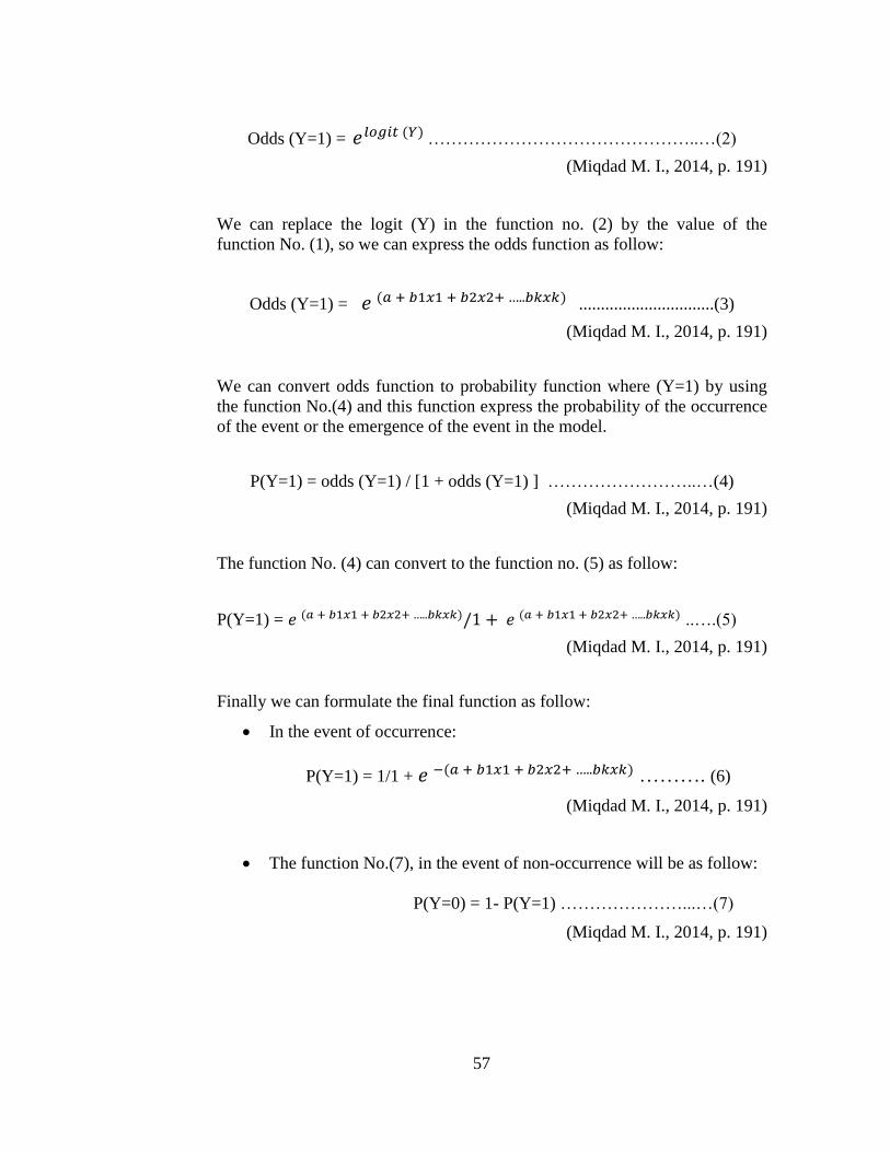
57
Odds (Y=1) = ………………………………………..…(2)
(Miqdad M. I., 2014, p. 191)
We can replace the logit (Y) in the function no. (2) by the value of the
function No. (1), so we can express the odds function as follow:
Odds (Y=1) = ...............................(3)
(Miqdad M. I., 2014, p. 191)
We can convert odds function to probability function where (Y=1) by using
the function No.(4) and this function express the probability of the occurrence
of the event or the emergence of the event in the model.
P(Y=1) = odds (Y=1) / [1 + odds (Y=1) ] ……………………..…(4)
(Miqdad M. I., 2014, p. 191)
The function No. (4) can convert to the function no. (5) as follow:
P(Y=1) = ..….(5)
(Miqdad M. I., 2014, p. 191)
Finally we can formulate the final function as follow:
In the event of occurrence:
P(Y=1) = 1/1 + ………. (6)
(Miqdad M. I., 2014, p. 191)
The function No.(7), in the event of non-occurrence will be as follow:
P(Y=0) = 1- P(Y=1) …………………...…(7)
(Miqdad M. I., 2014, p. 191)
58
2.4.2.3 Interpretation of The Results
The interpretation of the results is the most important step after the
analysis and there are two types of results uses:
A. To know the direction and existence of the relationship.
B. Predicting probability of an event occurrence.
2.4.2.4 How The Model Might Fit The Data
Chi2
test is the corresponding test for ―F‖ test in linear regression model
which used for testing how fit of the data in the model.
If chi2
value statistically significant in which the sig. level is less than 5%
then we can refuse the null hypothesis and accept the relationship exits
which means we accept the occurrence of the event by independent
variables used in the model (Miqdad M. I., 2014, p. 194).
If chi2
value is not statistically significant in which the sig. level is more
than 5% then we can accept the null hypothesis and reject the relationship
exits which means we reject the occurrence of the event by independent
variables used in the model.
59
Chapter Three
Study Methodology and Data Analysis
3.1 Study Methodology
3.2 Data Analysis
60
3. Chapter Three: Study Methodology and Data Analysis
The chapter three presents the methodology of the study in section one
which includes the study design, statistical tests, methods of data collection,
study population and study procedure. Also, this chapter at section two presents
the data analysis which includes descriptive statistics, testing the variables
normality, testing hypothesis. Finally presenting the models that have been
reached and their predictive ability.
3.1 Study Methodology
Section one presents study methodology which includes the study design,
statistical tests, methods of data collection, study population and study
procedures.
3.1.1 The Study Design
This study used the descriptive analytical methodology since it is the most
suitable for this type of study by depending on the descriptive approach in the
presentation of the theoretical aspect of the study then used the analytical approach
in the presentation of the practical aspects and finally conducting the necessary tests.
3.1.2 Statistical Tests
The statistical analyses and necessary tests were conducted on the available
financial data to test the study hypotheses and to measure the models accuracy rates
concerning corporate failure prediction. The statistical software, SPSS, is used to
analyze the inputs based on the data of the study through the following measures and
tests:
A. Frequencies and percentages were used.
B. Descriptive statistics were used.
C. Kolmogorov–Smirnov test to know the type of data if it follows a normal
distribution or not (1-sample Ks).
D. T-tests to explore differences between groups of variables.
E. Hosmer Lemeshow test for overall fit of logistic regression model.
F. Logistic analysis were used to build a failure prediction model.
G. Variance influence factor (VIF) to test multicollinearity problem.
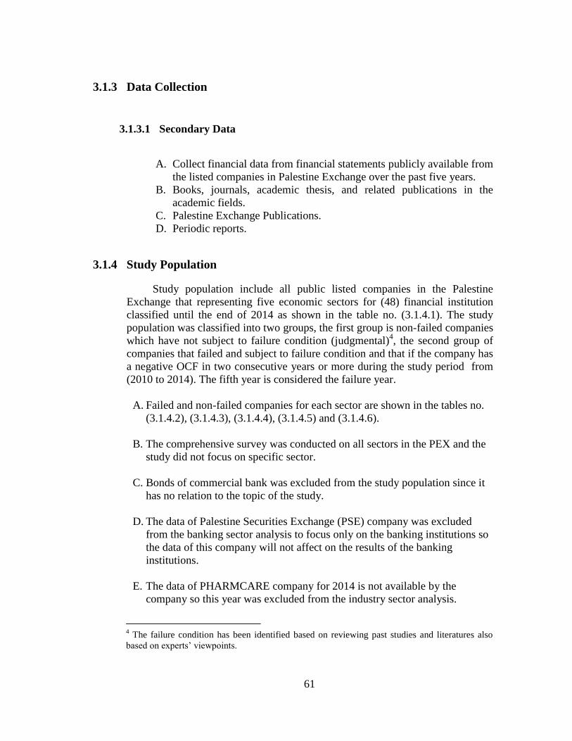
61
3.1.3 Data Collection
3.1.3.1 Secondary Data
A. Collect financial data from financial statements publicly available from
the listed companies in Palestine Exchange over the past five years.
B. Books, journals, academic thesis, and related publications in the
academic fields.
C. Palestine Exchange Publications.
D. Periodic reports.
3.1.4 Study Population
Study population include all public listed companies in the Palestine
Exchange that representing five economic sectors for (48) financial institution
classified until the end of 2014 as shown in the table no. (3.1.4.1). The study
population was classified into two groups, the first group is non-failed companies
which have not subject to failure condition (judgmental)4, the second group of
companies that failed and subject to failure condition and that if the company has
a negative OCF in two consecutive years or more during the study period from
(2010 to 2014). The fifth year is considered the failure year.
A. Failed and non-failed companies for each sector are shown in the tables no.
(3.1.4.2), (3.1.4.3), (3.1.4.4), (3.1.4.5) and (3.1.4.6).
B. The comprehensive survey was conducted on all sectors in the PEX and the
study did not focus on specific sector.
C. Bonds of commercial bank was excluded from the study population since it
has no relation to the topic of the study.
D. The data of Palestine Securities Exchange (PSE) company was excluded
from the banking sector analysis to focus only on the banking institutions so
the data of this company will not affect on the results of the banking
institutions.
E. The data of PHARMCARE company for 2014 is not available by the
company so this year was excluded from the industry sector analysis.
4 The failure condition has been identified based on reviewing past studies and literatures also
based on experts‘ viewpoints.
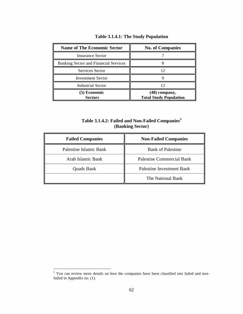
62
Table 3.1.4.1: The Study Population
Name of The Economic Sector No. of Companies
Insurance Sector 7
Banking Sector and Financial Services 8
Services Sector 12
Investment Sector 9
Industrial Sector 12
(5) Economic
Sectors
(48) company,
Total Study Population
Table 3.1.4.2: Failed and Non-Failed Companies5
(Banking Sector)
Failed Companies Non-Failed Companies
Palestine Islamic Bank Bank of Palestine
Arab Islamic Bank Palestine Commercial Bank
Quads Bank Palestine Investment Bank
The National Bank
5 You can review more details on how the companies have been classified into failed and non-
failed in Appendix no. (1).
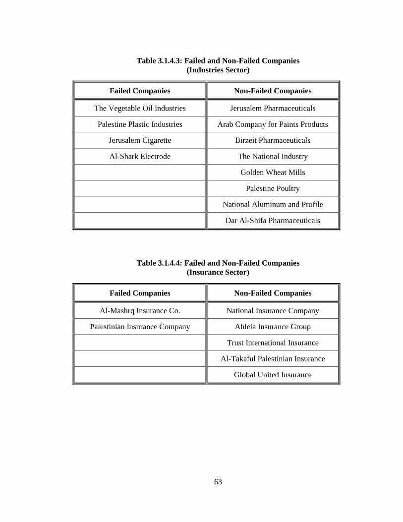
63
Table 3.1.4.3: Failed and Non-Failed Companies
(Industries Sector)
Failed Companies Non-Failed Companies
The Vegetable Oil Industries Jerusalem Pharmaceuticals
Palestine Plastic Industries Arab Company for Paints Products
Jerusalem Cigarette Birzeit Pharmaceuticals
Al-Shark Electrode The National Industry
Golden Wheat Mills
Palestine Poultry
National Aluminum and Profile
Dar Al-Shifa Pharmaceuticals
Table 3.1.4.4: Failed and Non-Failed Companies
(Insurance Sector)
Failed Companies Non-Failed Companies
Al-Mashrq Insurance Co. National Insurance Company
Palestinian Insurance Company Ahleia Insurance Group
Trust International Insurance
Al-Takaful Palestinian Insurance
Global United Insurance
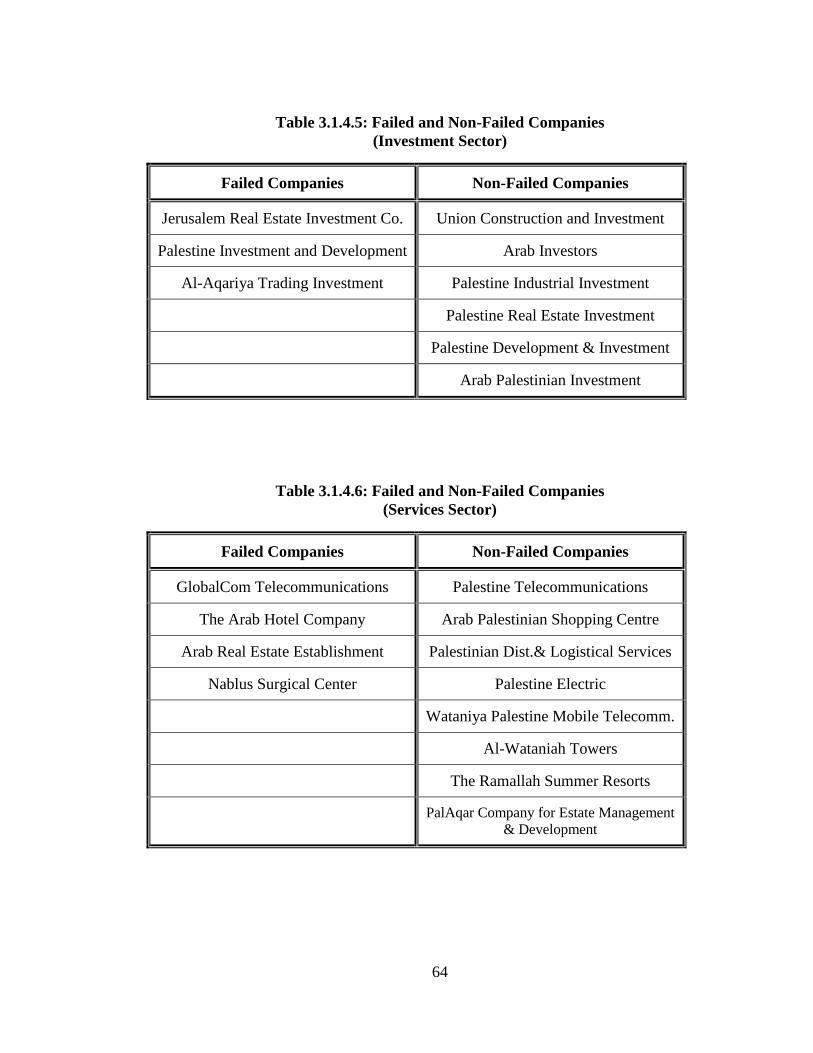
64
Table 3.1.4.5: Failed and Non-Failed Companies
(Investment Sector)
Failed Companies Non-Failed Companies
Jerusalem Real Estate Investment Co. Union Construction and Investment
Palestine Investment and Development Arab Investors
Al-Aqariya Trading Investment Palestine Industrial Investment
Palestine Real Estate Investment
Palestine Development & Investment
Arab Palestinian Investment
Table 3.1.4.6: Failed and Non-Failed Companies
(Services Sector)
Failed Companies Non-Failed Companies
GlobalCom Telecommunications Palestine Telecommunications
The Arab Hotel Company Arab Palestinian Shopping Centre
Arab Real Estate Establishment Palestinian Dist.& Logistical Services
Nablus Surgical Center Palestine Electric
Wataniya Palestine Mobile Telecomm.
Al-Wataniah Towers
The Ramallah Summer Resorts
PalAqar Company for Estate Management
& Development
65
3.1.5 Study Procedures
A. The financial statements collected for 48 company representing five
different economic sectors in PEX which include the balance sheet, income
statement and cash flow statement covering a period of five years from 2010
to 2014.
B. Financial statements consolidated in one form because of the different forms,
different currencies and different elements for each company. The
consolidated forms contained all necessary elements to conduct ratios
analysis.
C. The U.S dollar determined as common currency of the financial statements
for companies at common exchange rate = 3.8 NIS/$ and common exchange
rate = .7 $/JD
D. The financial ratios calculated by Ms Excel software.
E. The statistical significant ratios determined by SPSS-21 software.
3.1.6 Predictor Variables
Failure prediction models used accrual accounting-based measures.
Researchers in the past have used cash flow data but with mixed results. Cash
Shortage and bad financial performance are often-cited reasons for financial
distress.
Why cash flow? (Bhandari & Iyer, 2013, pp. 668-669)
Ever since accrual accounting system was adopted for recording and
reporting business transactions, balance sheets and income statements were the
main source of information for academics, analysts and investors for their
research and decision-making purposes. The importance of cash flow, though
intuitive was not realized until the accounting regulators and textbook authors
started emphasizing CFS. ―Cash is King‖ phrase is now widely understood and
respected. Obviously because cash is what buys things, pays wages and salaries;
services and pays debt; and compensates stockholders (owners) not accounting
income! Inadequate cash can lead to default on accrued payables and ultimate
bankruptcy. The most important and useful information in CFS is operating cash
flow (OCF). A business is supposed to operate profitably and generate cash. OCF
is that number! Another cash flow measure known as free cash flow (FCF) is
used by many academics and analysts. Although FCF is useful for internal
analysis and decision-making purposes, it is a vague concept because there are
many different versions of this measure. Computation and disclosure of FCF is
66
not mandated by accounting regulatory agencies whereas OCF is. OCF is clearly
defined, meticulously calculated and universally disclosed as a part of CFS.
The rationale for selecting these eleventh measures as explanatory variables is as
follows:
Operating cash flow divided by current liabilities (OCF/CL).
This ratio measures a firm‘s liquidity by comparing actual cash flow with
the short-term obligations. Lower the value of this ratio more the
likelihood of business failure. This ratio used by (Bhandari & Iyer, 2013),
(Rodgers, 2013) and (Matar & Obaidat, 2007).
Cash flow coverage of interest (OCF + INT + Tax/INT).
The numerator of this ratio is OCF plus interest and taxes paid. The
denominator consists of both short- and long-term interest. This ratio
measures a firm‘s ability to service (cover) interest obligation on debt. It
is similar to the times interest earned (TIE) ratio which is based on data
derived from the income statement. Higher the value of this ratio means
lessen the chance of default on interest payment by a firm (Bhandari &
Iyer, 2013, p. 670).
Operating cash flow margin (OCF/Sales).
This ratio is similar to traditional profit margin ratio. It is calculated by
dividing net sales into OCF, thereby measuring the ability of a firm to
translate sales into cash this ratio is a more appropriate measure of a
firm‘s operating profitability and liquidity as opposed to accrual
accounting-based profit margin ratio. There are at least four different
profit margin ratios depending upon which profit (gross profit, operating
profit, pre-tax profit or net profit) is in the numerator. But there is only
one OCF margin ratio. This is another reason why the proposed ratio is
more useful measure than net profit margin ratio (Bhandari & Iyer, 2013,
p. 670).
Operating cash flow return on total assets (OCF/Asset).
This ratio is similar to return on assets (ROA) but instead of net income,
cash flow from operation is used in the numerator. This ratio measures
cash generating ability of all the assets, i.e. assets provided by both
creditors and stockholders of the firm. (Bhandari & Iyer, 2013), (Rodgers,
2013) and (Matar & Obaidat, 2007) have used this ratio.
67
Quality of earning (EBIT/OCF).
The quality of earnings usually refers to the degree of conservatism in a
firm‘s reported earnings. The operating income (or earnings before
interest and taxes) divided by OCF is one such measure. A value less than
one signals that (accrual) income is of lesser quality and of impending
financial trouble (Bhandari & Iyer, 2013, p. 670).
Quick ratio (acid-test ratio).
This is a traditional but highly popular measure of corporate liquidity.
Current assets minus inventories are divided by current liabilities. The
―quick‖ assets are cash, marketable securities, receivables and pre-paid
items. A lower value of this ratio is associated with firm under distress.
Operating cash flow return on Equity (OCF/EQUITY).
This ratio is similar to return on equity (ROE) but instead of net income,
cash flow from operation is used in the numerator. This ratio measures
cash financed by stockholders.
Operating cash flow return on Net Income (OCF/N.I) used by
(Rodgers, 2013).
Operating cash flow return on current Assets (OCF/C.A) used by
(Rodgers, 2013).
Operating cash flow return on free cash flow (OCF/FCF) used by
(Rodgers, 2013).
Free cash flow on current liabilities (FCF/C.L) used by (Rodgers, 2013).
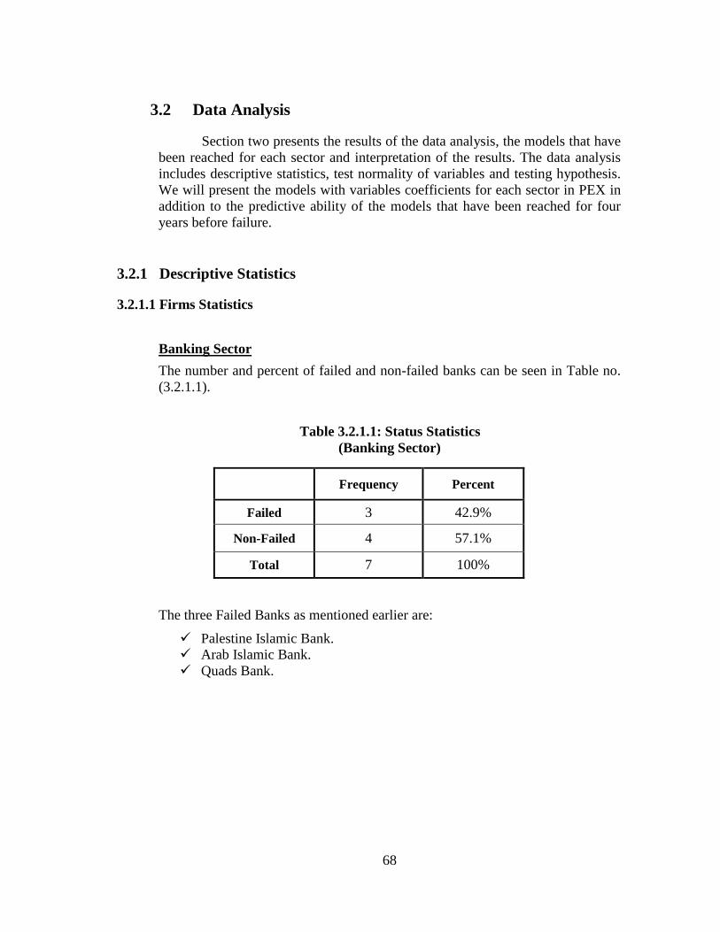
68
3.2 Data Analysis
Section two presents the results of the data analysis, the models that have
been reached for each sector and interpretation of the results. The data analysis
includes descriptive statistics, test normality of variables and testing hypothesis.
We will present the models with variables coefficients for each sector in PEX in
addition to the predictive ability of the models that have been reached for four
years before failure.
3.2.1 Descriptive Statistics
3.2.1.1 Firms Statistics
Banking Sector
The number and percent of failed and non-failed banks can be seen in Table no.
(3.2.1.1).
Table 3.2.1.1: Status Statistics
(Banking Sector)
Frequency Percent
Failed 3 42.9%
Non-Failed 4 57.1%
Total 7 100%
The three Failed Banks as mentioned earlier are:
Palestine Islamic Bank.
Arab Islamic Bank.
Quads Bank.
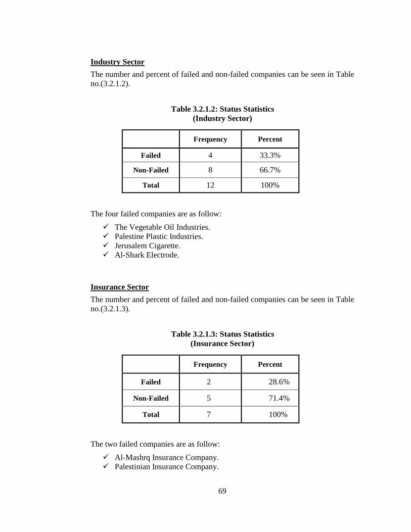
69
Industry Sector
The number and percent of failed and non-failed companies can be seen in Table
no.(3.2.1.2).
Table 3.2.1.2: Status Statistics
(Industry Sector)
Frequency Percent
Failed 4 33.3%
Non-Failed 8 66.7%
Total 12 100%
The four failed companies are as follow:
The Vegetable Oil Industries.
Palestine Plastic Industries.
Jerusalem Cigarette.
Al-Shark Electrode.
Insurance Sector
The number and percent of failed and non-failed companies can be seen in Table
no.(3.2.1.3).
Table 3.2.1.3: Status Statistics
(Insurance Sector)
Frequency Percent
Failed 2 28.6%
Non-Failed 5 71.4%
Total 7 100%
The two failed companies are as follow:
Al-Mashrq Insurance Company.
Palestinian Insurance Company.
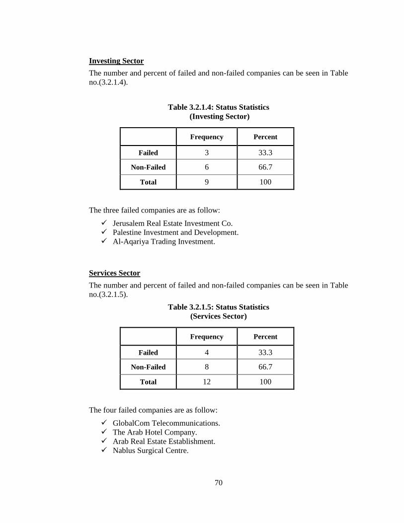
70
Investing Sector
The number and percent of failed and non-failed companies can be seen in Table
no.(3.2.1.4).
Table 3.2.1.4: Status Statistics
(Investing Sector)
Frequency Percent
Failed 3 33.3
Non-Failed 6 66.7
Total 9 100
The three failed companies are as follow:
Jerusalem Real Estate Investment Co.
Palestine Investment and Development.
Al-Aqariya Trading Investment.
Services Sector
The number and percent of failed and non-failed companies can be seen in Table
no.(3.2.1.5).
Table 3.2.1.5: Status Statistics
(Services Sector)
Frequency Percent
Failed 4 33.3
Non-Failed 8 66.7
Total 12 100
The four failed companies are as follow:
GlobalCom Telecommunications.
The Arab Hotel Company.
Arab Real Estate Establishment.
Nablus Surgical Centre.
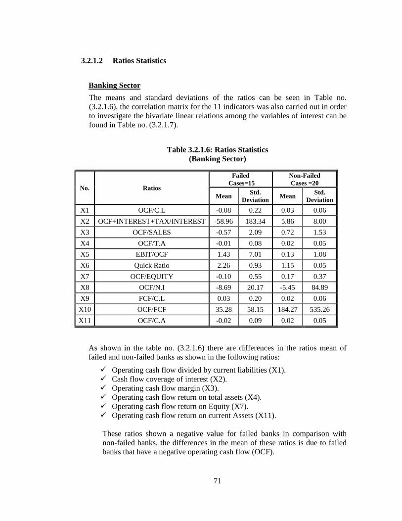
71
3.2.1.2 Ratios Statistics
Banking Sector
The means and standard deviations of the ratios can be seen in Table no.
(3.2.1.6), the correlation matrix for the 11 indicators was also carried out in order
to investigate the bivariate linear relations among the variables of interest can be
found in Table no. (3.2.1.7).
Table 3.2.1.6: Ratios Statistics
(Banking Sector)
No. Ratios
Failed
Cases=15
Non-Failed
Cases =20
Mean Std.
Deviation Mean
Std.
Deviation
X1 OCF/C.L -0.08 0.22 0.03 0.06
X2 OCF+INTEREST+TAX/INTEREST -58.96 183.34 5.86 8.00
X3 OCF/SALES -0.57 2.09 0.72 1.53
X4 OCF/T.A -0.01 0.08 0.02 0.05
X5 EBIT/OCF 1.43 7.01 0.13 1.08
X6 Quick Ratio 2.26 0.93 1.15 0.05
X7 OCF/EQUITY -0.10 0.55 0.17 0.37
X8 OCF/N.I -8.69 20.17 -5.45 84.89
X9 FCF/C.L 0.03 0.20 0.02 0.06
X10 OCF/FCF 35.28 58.15 184.27 535.26
X11 OCF/C.A -0.02 0.09 0.02 0.05
As shown in the table no. (3.2.1.6) there are differences in the ratios mean of
failed and non-failed banks as shown in the following ratios:
Operating cash flow divided by current liabilities (X1).
Cash flow coverage of interest (X2).
Operating cash flow margin (X3).
Operating cash flow return on total assets (X4).
Operating cash flow return on Equity (X7).
Operating cash flow return on current Assets (X11).
These ratios shown a negative value for failed banks in comparison with
non-failed banks, the differences in the mean of these ratios is due to failed
banks that have a negative operating cash flow (OCF).
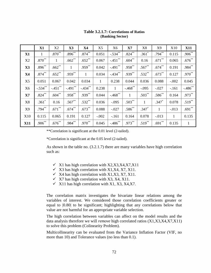
72
Table 3.2.1.7: Correlations of Ratios
(Banking Sector)
**Correlation is significant at the 0.01 level (2-tailed).
*Correlation is significant at the 0.05 level (2-tailed).
As shown in the table no. (3.2.1.7) there are many variables have high correlation
such as:
X1 has high correlation with X2,X3,X4,X7,X11
X3 has high correlation with X1,X4, X7, X11.
X4 has high correlation with X1,X3, X7, X11.
X7 has high correlation with X3, X4, X11.
X11 has high correlation with X1, X3, X4,X7.
The correlation matrix investigates the bivariate linear relations among the
variables of interest. We considered those correlation coefficients greater or
equal to |0.80| to be significant; highlighting that any correlations below that
value are not harmful for an appropriate variable selection.
The high correlation between variables can affect on the model results and the
data analysis therefore we will remove high correlated ratios (X1,X3,X4,X7,X11)
to solve this problem (Colinearity Problem).
Multicollinearity can be evaluated from the Variance Inflation Factor (VIF, no
more than 10) and Tolerance values (no less than 0.1).
X1 X2 X3 X4 X5 X6 X7 X8 X9 X10 X11
X1 1 .870**
.896**
.874**
0.051 -.534**
.824**
.361* .794
** 0.115 .906
**
X2 .870**
1 .662**
.652**
0.067 -.451**
.604**
0.16 .671**
0.065 .676**
X3 .896**
.662**
1 .959**
0.042 -.491**
.958**
.567**
.674**
0.191 .984**
X4 .874**
.652**
.959**
1 0.034 -.434**
.939**
.532**
.673**
0.127 .970**
X5 0.051 0.067 0.042 0.034 1 0.238 0.044 0.036 0.088 -.002 0.045
X6 -.534**
-.451**
-.491**
-.434**
0.238 1 -.468**
-.095 -.027 -.161 -.486**
X7 .824**
.604**
.958**
.939**
0.044 -.468**
1 .503**
.586**
0.164 .973**
X8 .361* 0.16 .567
** .532
** 0.036 -.095 .503
** 1 .347
* 0.078 .519
**
X9 .794**
.671**
.674**
.673**
0.088 -.027 .586**
.347* 1 -.013 .691
**
X10 0.115 0.065 0.191 0.127 -.002 -.161 0.164 0.078 -.013 1 0.135
X11 .906**
.676**
.984**
.970**
0.045 -.486**
.973**
.519**
.691**
0.135 1
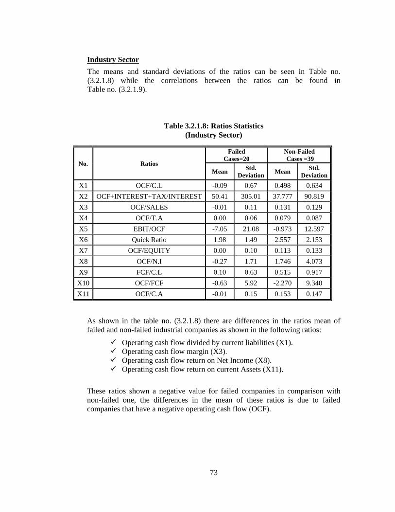
73
Industry Sector
The means and standard deviations of the ratios can be seen in Table no.
(3.2.1.8) while the correlations between the ratios can be found in
Table no. (3.2.1.9).
Table 3.2.1.8: Ratios Statistics
(Industry Sector)
No. Ratios
Failed
Cases=20
Non-Failed
Cases =39
Mean Std.
Deviation Mean
Std.
Deviation
X1 OCF/C.L -0.09 0.67 0.498 0.634
X2 OCF+INTEREST+TAX/INTEREST 50.41 305.01 37.777 90.819
X3 OCF/SALES -0.01 0.11 0.131 0.129
X4 OCF/T.A 0.00 0.06 0.079 0.087
X5 EBIT/OCF -7.05 21.08 -0.973 12.597
X6 Quick Ratio 1.98 1.49 2.557 2.153
X7 OCF/EQUITY 0.00 0.10 0.113 0.133
X8 OCF/N.I -0.27 1.71 1.746 4.073
X9 FCF/C.L 0.10 0.63 0.515 0.917
X10 OCF/FCF -0.63 5.92 -2.270 9.340
X11 OCF/C.A -0.01 0.15 0.153 0.147
As shown in the table no. (3.2.1.8) there are differences in the ratios mean of
failed and non-failed industrial companies as shown in the following ratios:
Operating cash flow divided by current liabilities (X1).
Operating cash flow margin (X3).
Operating cash flow return on Net Income (X8).
Operating cash flow return on current Assets (X11).
These ratios shown a negative value for failed companies in comparison with
non-failed one, the differences in the mean of these ratios is due to failed
companies that have a negative operating cash flow (OCF).
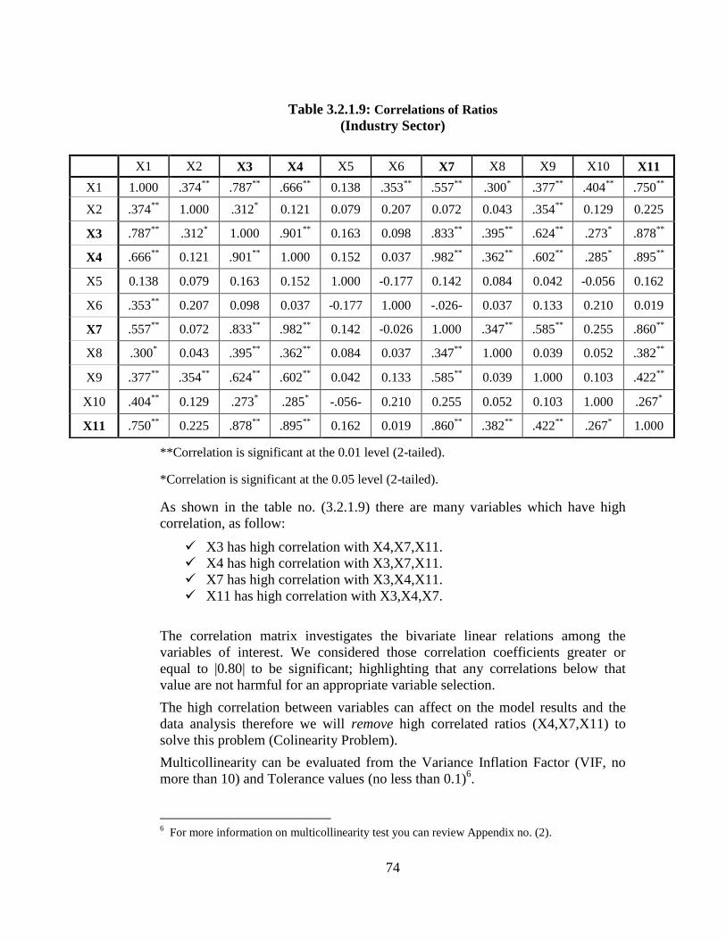
74
Table 3.2.1.9: Correlations of Ratios
(Industry Sector)
**Correlation is significant at the 0.01 level (2-tailed).
*Correlation is significant at the 0.05 level (2-tailed).
As shown in the table no. (3.2.1.9) there are many variables which have high
correlation, as follow:
X3 has high correlation with X4,X7,X11.
X4 has high correlation with X3,X7,X11.
X7 has high correlation with X3,X4,X11.
X11 has high correlation with X3,X4,X7.
The correlation matrix investigates the bivariate linear relations among the
variables of interest. We considered those correlation coefficients greater or
equal to |0.80| to be significant; highlighting that any correlations below that
value are not harmful for an appropriate variable selection.
The high correlation between variables can affect on the model results and the
data analysis therefore we will remove high correlated ratios (X4,X7,X11) to
solve this problem (Colinearity Problem).
Multicollinearity can be evaluated from the Variance Inflation Factor (VIF, no
more than 10) and Tolerance values (no less than 0.1)6.
6 For more information on multicollinearity test you can review Appendix no. (2).
X1 X2 X3 X4 X5 X6 X7 X8 X9 X10 X11
X1 1.000 .374**
.787**
.666**
0.138 .353**
.557**
.300* .377
** .404
** .750
**
X2 .374**
1.000 .312* 0.121 0.079 0.207 0.072 0.043 .354
** 0.129 0.225
X3 .787**
.312* 1.000 .901
** 0.163 0.098 .833
** .395
** .624
** .273
* .878
**
X4 .666**
0.121 .901**
1.000 0.152 0.037 .982**
.362**
.602**
.285* .895
**
X5 0.138 0.079 0.163 0.152 1.000 -0.177 0.142 0.084 0.042 -0.056 0.162
X6 .353**
0.207 0.098 0.037 -0.177 1.000 -.026- 0.037 0.133 0.210 0.019
X7 .557**
0.072 .833**
.982**
0.142 -0.026 1.000 .347**
.585**
0.255 .860**
X8 .300* 0.043 .395
** .362
** 0.084 0.037 .347
** 1.000 0.039 0.052 .382
**
X9 .377**
.354**
.624**
.602**
0.042 0.133 .585**
0.039 1.000 0.103 .422**
X10 .404**
0.129 .273* .285
* -.056- 0.210 0.255 0.052 0.103 1.000 .267
*
X11 .750**
0.225 .878**
.895**
0.162 0.019 .860**
.382**
.422**
.267* 1.000
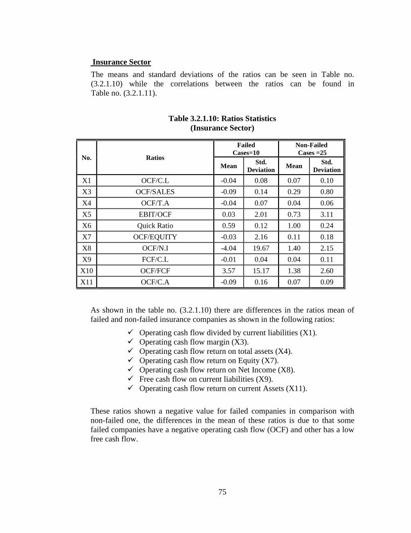
75
Insurance Sector
The means and standard deviations of the ratios can be seen in Table no.
(3.2.1.10) while the correlations between the ratios can be found in
Table no. (3.2.1.11).
Table 3.2.1.10: Ratios Statistics
(Insurance Sector)
No. Ratios
Failed
Cases=10
Non-Failed
Cases =25
Mean Std.
Deviation Mean
Std.
Deviation
X1 OCF/C.L -0.04 0.08 0.07 0.10
X3 OCF/SALES -0.09 0.14 0.29 0.80
X4 OCF/T.A -0.04 0.07 0.04 0.06
X5 EBIT/OCF 0.03 2.01 0.73 3.11
X6 Quick Ratio 0.59 0.12 1.00 0.24
X7 OCF/EQUITY -0.03 2.16 0.11 0.18
X8 OCF/N.I -4.04 19.67 1.40 2.15
X9 FCF/C.L -0.01 0.04 0.04 0.11
X10 OCF/FCF 3.57 15.17 1.38 2.60
X11 OCF/C.A -0.09 0.16 0.07 0.09
As shown in the table no. (3.2.1.10) there are differences in the ratios mean of
failed and non-failed insurance companies as shown in the following ratios:
Operating cash flow divided by current liabilities (X1).
Operating cash flow margin (X3).
Operating cash flow return on total assets (X4).
Operating cash flow return on Equity (X7).
Operating cash flow return on Net Income (X8).
Free cash flow on current liabilities (X9).
Operating cash flow return on current Assets (X11).
These ratios shown a negative value for failed companies in comparison with
non-failed one, the differences in the mean of these ratios is due to that some
failed companies have a negative operating cash flow (OCF) and other has a low
free cash flow.
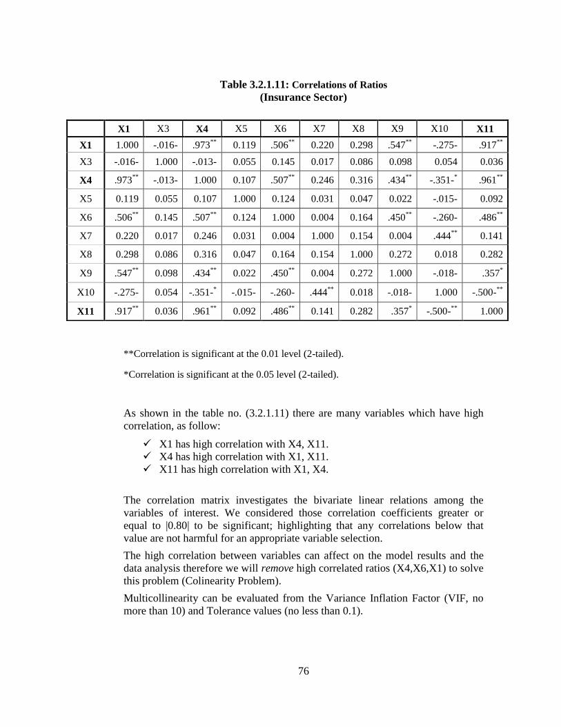
76
Table 3.2.1.11: Correlations of Ratios
(Insurance Sector)
**Correlation is significant at the 0.01 level (2-tailed).
*Correlation is significant at the 0.05 level (2-tailed).
As shown in the table no. (3.2.1.11) there are many variables which have high
correlation, as follow:
X1 has high correlation with X4, X11.
X4 has high correlation with X1, X11.
X11 has high correlation with X1, X4.
The correlation matrix investigates the bivariate linear relations among the
variables of interest. We considered those correlation coefficients greater or
equal to |0.80| to be significant; highlighting that any correlations below that
value are not harmful for an appropriate variable selection.
The high correlation between variables can affect on the model results and the
data analysis therefore we will remove high correlated ratios (X4,X6,X1) to solve
this problem (Colinearity Problem).
Multicollinearity can be evaluated from the Variance Inflation Factor (VIF, no
more than 10) and Tolerance values (no less than 0.1).
X1 X3 X4 X5 X6 X7 X8 X9 X10 X11
X1 1.000 -.016- .973**
0.119 .506**
0.220 0.298 .547**
-.275- .917**
X3 -.016- 1.000 -.013- 0.055 0.145 0.017 0.086 0.098 0.054 0.036
X4 .973**
-.013- 1.000 0.107 .507**
0.246 0.316 .434**
-.351-* .961
**
X5 0.119 0.055 0.107 1.000 0.124 0.031 0.047 0.022 -.015- 0.092
X6 .506**
0.145 .507**
0.124 1.000 0.004 0.164 .450**
-.260- .486**
X7 0.220 0.017 0.246 0.031 0.004 1.000 0.154 0.004 .444**
0.141
X8 0.298 0.086 0.316 0.047 0.164 0.154 1.000 0.272 0.018 0.282
X9 .547**
0.098 .434**
0.022 .450**
0.004 0.272 1.000 -.018- .357*
X10 -.275- 0.054 -.351-* -.015- -.260- .444
** 0.018 -.018- 1.000 -.500-
**
X11 .917**
0.036 .961**
0.092 .486**
0.141 0.282 .357* -.500-
** 1.000
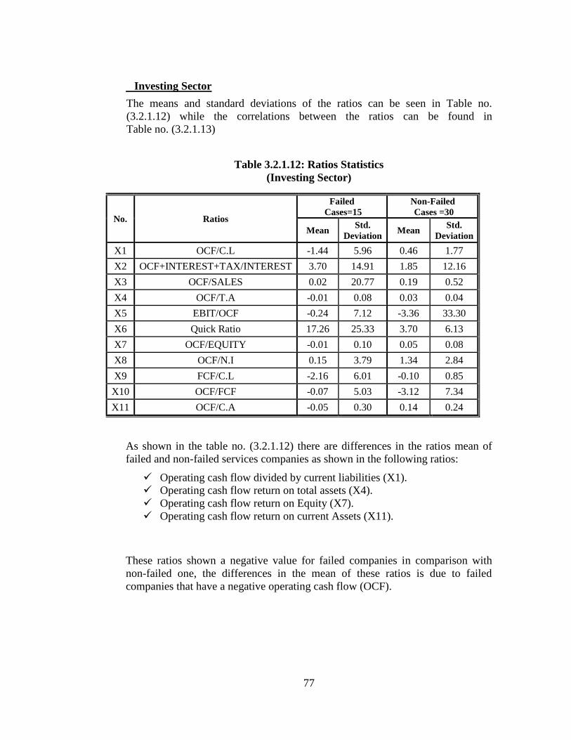
77
Investing Sector
The means and standard deviations of the ratios can be seen in Table no.
(3.2.1.12) while the correlations between the ratios can be found in
Table no. (3.2.1.13)
Table 3.2.1.12: Ratios Statistics
(Investing Sector)
No. Ratios
Failed
Cases=15
Non-Failed
Cases =30
Mean Std.
Deviation Mean
Std.
Deviation
X1 OCF/C.L -1.44 5.96 0.46 1.77
X2 OCF+INTEREST+TAX/INTEREST 3.70 14.91 1.85 12.16
X3 OCF/SALES 0.02 20.77 0.19 0.52
X4 OCF/T.A -0.01 0.08 0.03 0.04
X5 EBIT/OCF -0.24 7.12 -3.36 33.30
X6 Quick Ratio 17.26 25.33 3.70 6.13
X7 OCF/EQUITY -0.01 0.10 0.05 0.08
X8 OCF/N.I 0.15 3.79 1.34 2.84
X9 FCF/C.L -2.16 6.01 -0.10 0.85
X10 OCF/FCF -0.07 5.03 -3.12 7.34
X11 OCF/C.A -0.05 0.30 0.14 0.24
As shown in the table no. (3.2.1.12) there are differences in the ratios mean of
failed and non-failed services companies as shown in the following ratios:
Operating cash flow divided by current liabilities (X1).
Operating cash flow return on total assets (X4).
Operating cash flow return on Equity (X7).
Operating cash flow return on current Assets (X11).
These ratios shown a negative value for failed companies in comparison with
non-failed one, the differences in the mean of these ratios is due to failed
companies that have a negative operating cash flow (OCF).
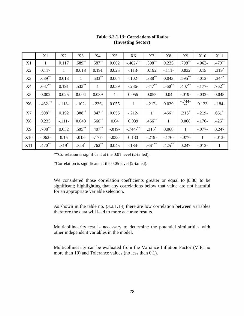
78
Table 3.2.1.13: Correlations of Ratios
(Investing Sector)
**Correlation is significant at the 0.01 level (2-tailed).
*Correlation is significant at the 0.05 level (2-tailed).
We considered those correlation coefficients greater or equal to |0.80| to be
significant; highlighting that any correlations below that value are not harmful
for an appropriate variable selection.
As shown in the table no. (3.2.1.13) there are low correlation between variables
therefore the data will lead to more accurate results.
Multicollinearity test is necessary to determine the potential similarities with
other independent variables in the model.
Multicollinearity can be evaluated from the Variance Inflation Factor (VIF, no
more than 10) and Tolerance values (no less than 0.1).
X1 X2 X3 X4 X5 X6 X7 X8 X9 X10 X11
X1 1 0.117 .689**
.687**
0.002 -.462-**
.508**
0.235 .708**
-.062- .470**
X2 0.117 1 0.013 0.191 0.025 -.113- 0.192 -.111- 0.032 0.15 .319*
X3 .689**
0.013 1 .533**
0.004 -.102- .388**
0.043 .595**
-.013- .344*
X4 .687**
0.191 .533**
1 0.039 -.236- .847**
.560**
.407**
-.177- .762**
X5 0.002 0.025 0.004 0.039 1 0.055 0.055 0.04 -.019- -.033- 0.045
X6 -.462-**
-.113- -.102- -.236- 0.055 1 -.212- 0.039 -.744-
**
0.133 -.184-
X7 .508**
0.192 .388**
.847**
0.055 -.212- 1 .466**
.315* -.219- .661
**
X8 0.235 -.111- 0.043 .560**
0.04 0.039 .466**
1 0.068 -.176- .425**
X9 .708**
0.032 .595**
.407**
-.019- -.744-**
.315* 0.068 1 -.077- 0.247
X10 -.062- 0.15 -.013- -.177- -.033- 0.133 -.219- -.176- -.077- 1 -.013-
X11 .470**
.319* .344
* .762
** 0.045 -.184- .661
** .425
** 0.247 -.013- 1
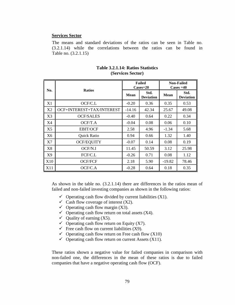
79
Services Sector
The means and standard deviations of the ratios can be seen in Table no.
(3.2.1.14) while the correlations between the ratios can be found in
Table no. (3.2.1.15)
Table 3.2.1.14: Ratios Statistics
(Services Sector)
No. Ratios
Failed
Cases=20
Non-Failed
Cases =40
Mean Std.
Deviation Mean
Std.
Deviation
X1 OCF/C.L -0.20 0.36 0.35 0.53
X2 OCF+INTEREST+TAX/INTEREST -14.16 42.34 25.67 49.08
X3 OCF/SALES -0.40 0.64 0.22 0.34
X4 OCF/T.A -0.04 0.08 0.06 0.10
X5 EBIT/OCF 2.58 4.96 -1.34 5.68
X6 Quick Ratio 0.94 0.66 1.32 1.40
X7 OCF/EQUITY -0.07 0.14 0.08 0.19
X8 OCF/N.I 11.45 50.59 3.12 25.98
X9 FCF/C.L -0.26 0.71 0.08 1.12
X10 OCF/FCF 2.18 5.90 -19.82 78.46
X11 OCF/C.A -0.28 0.64 0.18 0.35
As shown in the table no. (3.2.1.14) there are differences in the ratios mean of
failed and non-failed investing companies as shown in the following ratios:
Operating cash flow divided by current liabilities (X1).
Cash flow coverage of interest (X2).
Operating cash flow margin (X3).
Operating cash flow return on total assets (X4).
Quality of earning (X5).
Operating cash flow return on Equity (X7).
Free cash flow on current liabilities (X9).
Operating cash flow return on Free cash flow (X10)
Operating cash flow return on current Assets (X11).
These ratios shown a negative value for failed companies in comparison with
non-failed one, the differences in the mean of these ratios is due to failed
companies that have a negative operating cash flow (OCF).
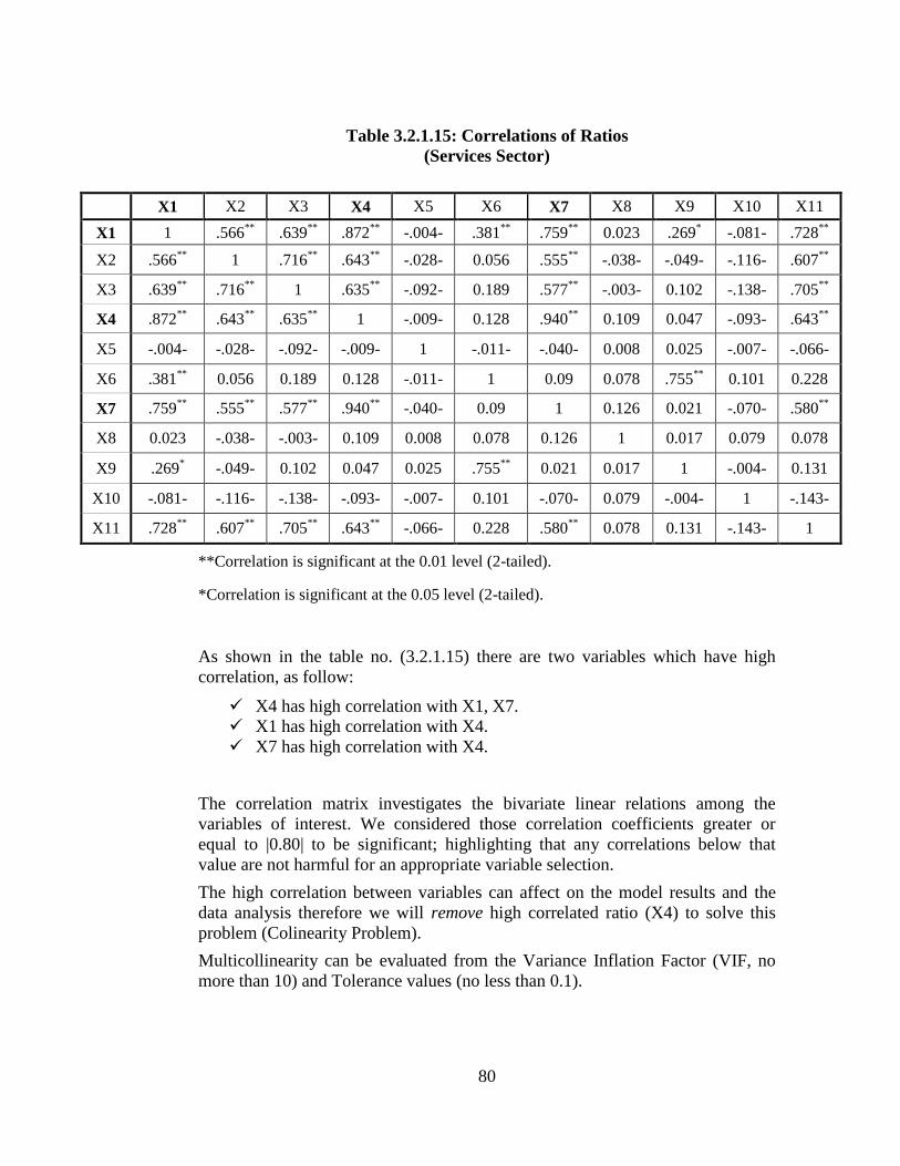
80
Table 3.2.1.15: Correlations of Ratios
(Services Sector)
**Correlation is significant at the 0.01 level (2-tailed).
*Correlation is significant at the 0.05 level (2-tailed).
As shown in the table no. (3.2.1.15) there are two variables which have high
correlation, as follow:
X4 has high correlation with X1, X7.
X1 has high correlation with X4.
X7 has high correlation with X4.
The correlation matrix investigates the bivariate linear relations among the
variables of interest. We considered those correlation coefficients greater or
equal to |0.80| to be significant; highlighting that any correlations below that
value are not harmful for an appropriate variable selection.
The high correlation between variables can affect on the model results and the
data analysis therefore we will remove high correlated ratio (X4) to solve this
problem (Colinearity Problem).
Multicollinearity can be evaluated from the Variance Inflation Factor (VIF, no
more than 10) and Tolerance values (no less than 0.1).
X1 X2 X3 X4 X5 X6 X7 X8 X9 X10 X11
X1 1 .566**
.639**
.872**
-.004- .381**
.759**
0.023 .269* -.081- .728
**
X2 .566**
1 .716**
.643**
-.028- 0.056 .555**
-.038- -.049- -.116- .607**
X3 .639**
.716**
1 .635**
-.092- 0.189 .577**
-.003- 0.102 -.138- .705**
X4 .872**
.643**
.635**
1 -.009- 0.128 .940**
0.109 0.047 -.093- .643**
X5 -.004- -.028- -.092- -.009- 1 -.011- -.040- 0.008 0.025 -.007- -.066-
X6 .381**
0.056 0.189 0.128 -.011- 1 0.09 0.078 .755**
0.101 0.228
X7 .759**
.555**
.577**
.940**
-.040- 0.09 1 0.126 0.021 -.070- .580**
X8 0.023 -.038- -.003- 0.109 0.008 0.078 0.126 1 0.017 0.079 0.078
X9 .269* -.049- 0.102 0.047 0.025 .755
** 0.021 0.017 1 -.004- 0.131
X10 -.081- -.116- -.138- -.093- -.007- 0.101 -.070- 0.079 -.004- 1 -.143-
X11 .728**
.607**
.705**
.643**
-.066- 0.228 .580**
0.078 0.131 -.143- 1
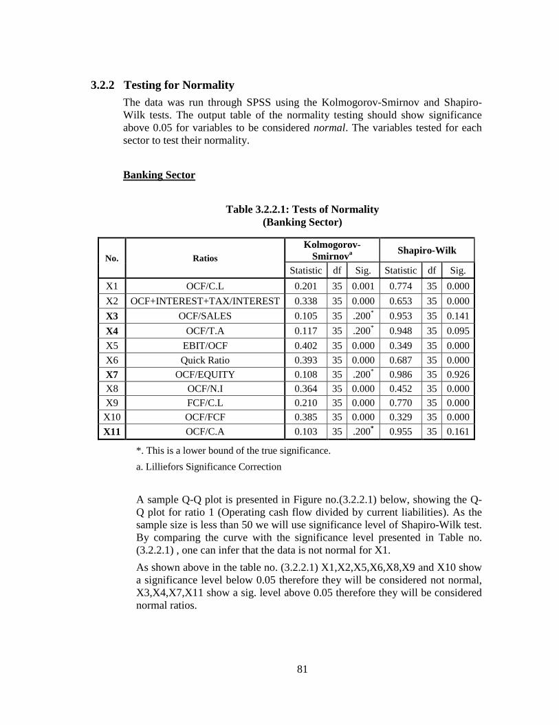
81
3.2.2 Testing for Normality
The data was run through SPSS using the Kolmogorov-Smirnov and Shapiro-
Wilk tests. The output table of the normality testing should show significance
above 0.05 for variables to be considered normal. The variables tested for each
sector to test their normality.
Banking Sector
Table 3.2.2.1: Tests of Normality
(Banking Sector)
No. Ratios
Kolmogorov-
Smirnova
Shapiro-Wilk
Statistic df Sig. Statistic df Sig.
X1 OCF/C.L 0.201 35 0.001 0.774 35 0.000
X2 OCF+INTEREST+TAX/INTEREST 0.338 35 0.000 0.653 35 0.000
X3 OCF/SALES 0.105 35 .200* 0.953 35 0.141
X4 OCF/T.A 0.117 35 .200* 0.948 35 0.095
X5 EBIT/OCF 0.402 35 0.000 0.349 35 0.000
X6 Quick Ratio 0.393 35 0.000 0.687 35 0.000
X7 OCF/EQUITY 0.108 35 .200* 0.986 35 0.926
X8 OCF/N.I 0.364 35 0.000 0.452 35 0.000
X9 FCF/C.L 0.210 35 0.000 0.770 35 0.000
X10 OCF/FCF 0.385 35 0.000 0.329 35 0.000
X11 OCF/C.A 0.103 35 .200* 0.955 35 0.161
*. This is a lower bound of the true significance.
a. Lilliefors Significance Correction
A sample Q-Q plot is presented in Figure no.(3.2.2.1) below, showing the Q-
Q plot for ratio 1 (Operating cash flow divided by current liabilities). As the
sample size is less than 50 we will use significance level of Shapiro-Wilk test.
By comparing the curve with the significance level presented in Table no.
(3.2.2.1) , one can infer that the data is not normal for X1.
As shown above in the table no. (3.2.2.1) X1,X2,X5,X6,X8,X9 and X10 show
a significance level below 0.05 therefore they will be considered not normal,
X3,X4,X7,X11 show a sig. level above 0.05 therefore they will be considered
normal ratios.
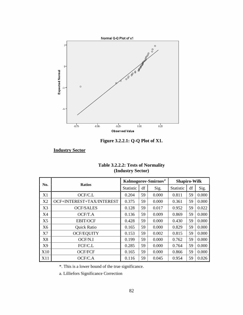
82
Figure 3.2.2.1: Q-Q Plot of X1.
Industry Sector
Table 3.2.2.2: Tests of Normality
(Industry Sector)
No. Ratios Kolmogorov-Smirnov
a Shapiro-Wilk
Statistic df Sig. Statistic df Sig.
X1 OCF/C.L 0.204 59 0.000 0.811 59 0.000
X2 OCF+INTEREST+TAX/INTEREST 0.375 59 0.000 0.361 59 0.000
X3 OCF/SALES 0.128 59 0.017 0.952 59 0.022
X4 OCF/T.A 0.136 59 0.009 0.869 59 0.000
X5 EBIT/OCF 0.428 59 0.000 0.430 59 0.000
X6 Quick Ratio 0.165 59 0.000 0.829 59 0.000
X7 OCF/EQUITY 0.153 59 0.002 0.815 59 0.000
X8 OCF/N.I 0.199 59 0.000 0.762 59 0.000
X9 FCF/C.L 0.285 59 0.000 0.764 59 0.000
X10 OCF/FCF 0.165 59 0.000 0.866 59 0.000
X11 OCF/C.A 0.116 59 0.045 0.954 59 0.026
*. This is a lower bound of the true significance.
a. Lilliefors Significance Correction
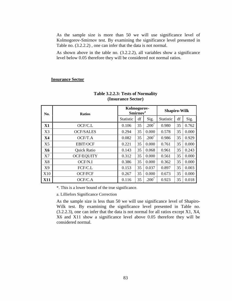
83
As the sample size is more than 50 we will use significance level of
Kolmogorov-Smirnov test. By examining the significance level presented in
Table no. (3.2.2.2) , one can infer that the data is not normal.
As shown above in the table no. (3.2.2.2), all variables show a significance
level below 0.05 therefore they will be considered not normal ratios.
Insurance Sector
Table 3.2.2.3: Tests of Normality
(Insurance Sector)
No. Ratios
Kolmogorov-
Smirnova
Shapiro-Wilk
Statistic df Sig. Statistic df Sig.
X1 OCF/C.L 0.106 35 .200* 0.980 35 0.762
X3 OCF/SALES 0.294 35 0.000 0.578 35 0.000
X4 OCF/T.A 0.082 35 .200* 0.986 35 0.929
X5 EBIT/OCF 0.221 35 0.000 0.761 35 0.000
X6 Quick Ratio 0.143 35 0.068 0.961 35 0.243
X7 OCF/EQUITY 0.312 35 0.000 0.561 35 0.000
X8 OCF/N.I 0.386 35 0.000 0.362 35 0.000
X9 FCF/C.L 0.153 35 0.037 0.897 35 0.003
X10 OCF/FCF 0.267 35 0.000 0.673 35 0.000
X11 OCF/C.A 0.116 35 .200* 0.923 35 0.018
*. This is a lower bound of the true significance.
a. Lilliefors Significance Correction
As the sample size is less than 50 we will use significance level of Shapiro-
Wilk test. By examining the significance level presented in Table no.
(3.2.2.3), one can infer that the data is not normal for all ratios except X1, X4,
X6 and X11 show a significance level above 0.05 therefore they will be
considered normal.
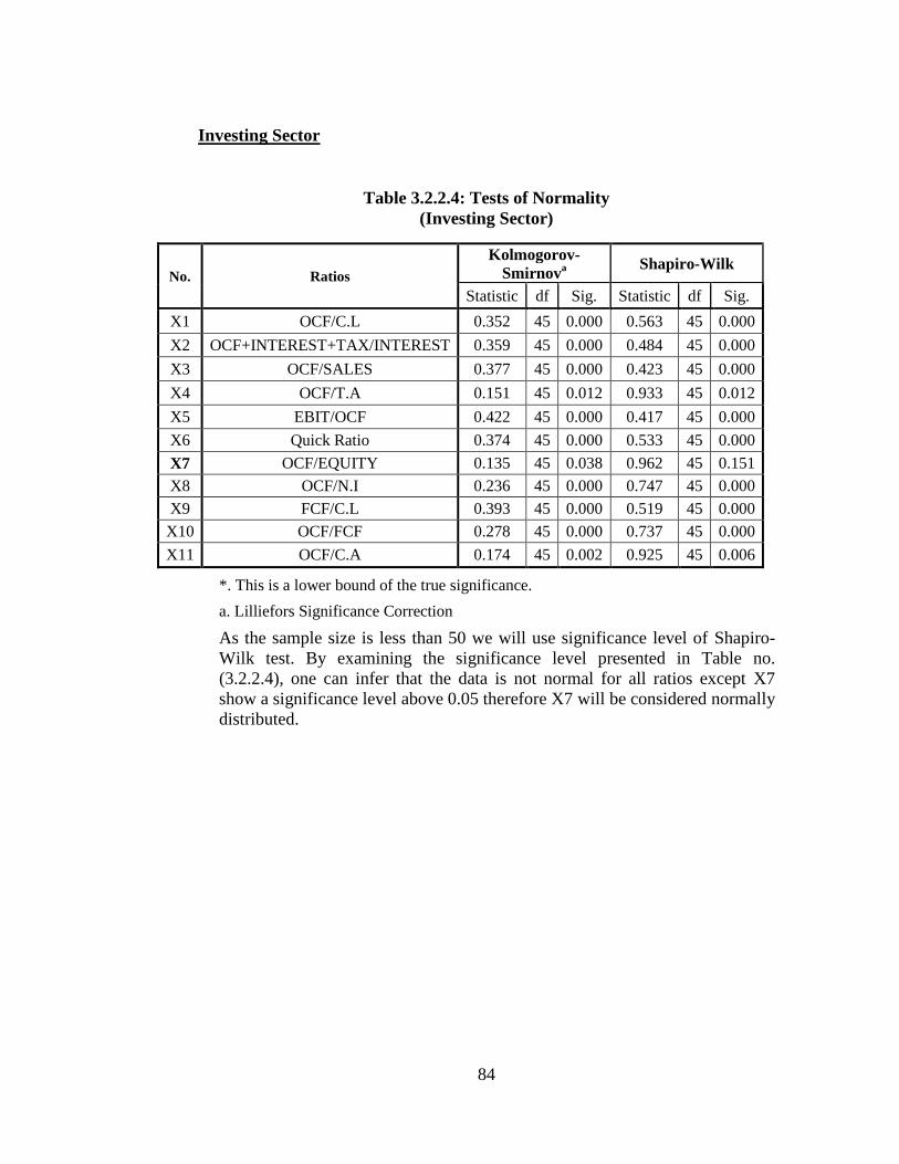
84
Investing Sector
Table 3.2.2.4: Tests of Normality
(Investing Sector)
No. Ratios
Kolmogorov-
Smirnova
Shapiro-Wilk
Statistic df Sig. Statistic df Sig.
X1 OCF/C.L 0.352 45 0.000 0.563 45 0.000
X2 OCF+INTEREST+TAX/INTEREST 0.359 45 0.000 0.484 45 0.000
X3 OCF/SALES 0.377 45 0.000 0.423 45 0.000
X4 OCF/T.A 0.151 45 0.012 0.933 45 0.012
X5 EBIT/OCF 0.422 45 0.000 0.417 45 0.000
X6 Quick Ratio 0.374 45 0.000 0.533 45 0.000
X7 OCF/EQUITY 0.135 45 0.038 0.962 45 0.151
X8 OCF/N.I 0.236 45 0.000 0.747 45 0.000
X9 FCF/C.L 0.393 45 0.000 0.519 45 0.000
X10 OCF/FCF 0.278 45 0.000 0.737 45 0.000
X11 OCF/C.A 0.174 45 0.002 0.925 45 0.006
*. This is a lower bound of the true significance.
a. Lilliefors Significance Correction
As the sample size is less than 50 we will use significance level of Shapiro-
Wilk test. By examining the significance level presented in Table no.
(3.2.2.4), one can infer that the data is not normal for all ratios except X7
show a significance level above 0.05 therefore X7 will be considered normally
distributed.
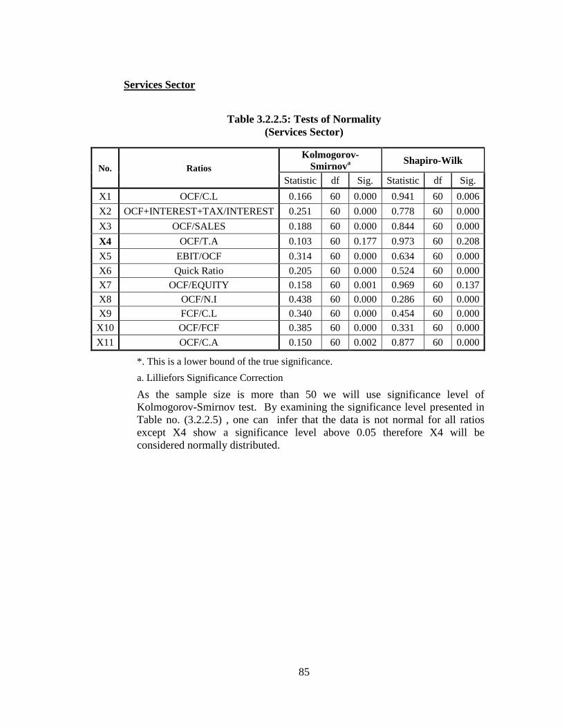
85
Services Sector
Table 3.2.2.5: Tests of Normality
(Services Sector)
No. Ratios
Kolmogorov-
Smirnova
Shapiro-Wilk
Statistic df Sig. Statistic df Sig.
X1 OCF/C.L 0.166 60 0.000 0.941 60 0.006
X2 OCF+INTEREST+TAX/INTEREST 0.251 60 0.000 0.778 60 0.000
X3 OCF/SALES 0.188 60 0.000 0.844 60 0.000
X4 OCF/T.A 0.103 60 0.177 0.973 60 0.208
X5 EBIT/OCF 0.314 60 0.000 0.634 60 0.000
X6 Quick Ratio 0.205 60 0.000 0.524 60 0.000
X7 OCF/EQUITY 0.158 60 0.001 0.969 60 0.137
X8 OCF/N.I 0.438 60 0.000 0.286 60 0.000
X9 FCF/C.L 0.340 60 0.000 0.454 60 0.000
X10 OCF/FCF 0.385 60 0.000 0.331 60 0.000
X11 OCF/C.A 0.150 60 0.002 0.877 60 0.000
*. This is a lower bound of the true significance.
a. Lilliefors Significance Correction
As the sample size is more than 50 we will use significance level of
Kolmogorov-Smirnov test. By examining the significance level presented in
Table no. (3.2.2.5) , one can infer that the data is not normal for all ratios
except X4 show a significance level above 0.05 therefore X4 will be
considered normally distributed.
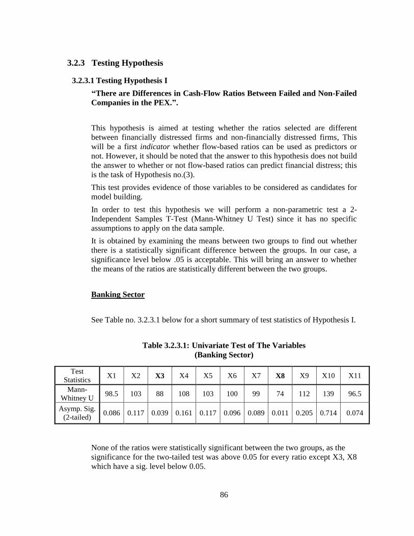
86
3.2.3 Testing Hypothesis
3.2.3.1 Testing Hypothesis I
“There are Differences in Cash-Flow Ratios Between Failed and Non-Failed
Companies in the PEX.”.
This hypothesis is aimed at testing whether the ratios selected are different
between financially distressed firms and non-financially distressed firms, This
will be a first indicator whether flow-based ratios can be used as predictors or
not. However, it should be noted that the answer to this hypothesis does not build
the answer to whether or not flow-based ratios can predict financial distress; this
is the task of Hypothesis no.(3).
This test provides evidence of those variables to be considered as candidates for
model building.
In order to test this hypothesis we will perform a non-parametric test a 2-
Independent Samples T-Test (Mann-Whitney U Test) since it has no specific
assumptions to apply on the data sample.
It is obtained by examining the means between two groups to find out whether
there is a statistically significant difference between the groups. In our case, a
significance level below .05 is acceptable. This will bring an answer to whether
the means of the ratios are statistically different between the two groups.
Banking Sector
See Table no. 3.2.3.1 below for a short summary of test statistics of Hypothesis I.
Table 3.2.3.1: Univariate Test of The Variables
(Banking Sector)
Test
Statistics X1 X2 X3 X4 X5 X6 X7 X8 X9 X10 X11
Mann-
Whitney U 98.5 103 88 108 103 100 99 74 112 139 96.5
Asymp. Sig.
(2-tailed) 0.086 0.117 0.039 0.161 0.117 0.096 0.089 0.011 0.205 0.714 0.074
None of the ratios were statistically significant between the two groups, as the
significance for the two-tailed test was above 0.05 for every ratio except X3, X8
which have a sig. level below 0.05.
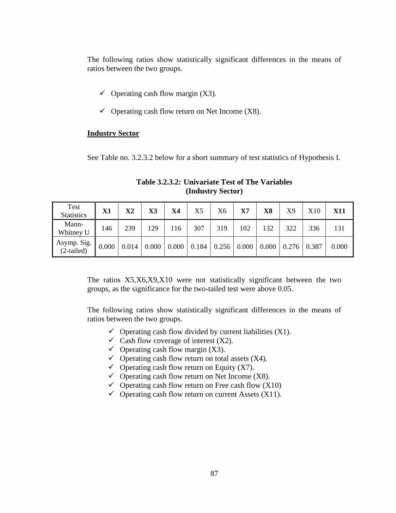
87
The following ratios show statistically significant differences in the means of
ratios between the two groups.
Operating cash flow margin (X3).
Operating cash flow return on Net Income (X8).
Industry Sector
See Table no. 3.2.3.2 below for a short summary of test statistics of Hypothesis I.
Table 3.2.3.2: Univariate Test of The Variables
(Industry Sector)
Test
Statistics X1 X2 X3 X4 X5 X6 X7 X8 X9 X10 X11
Mann-
Whitney U 146 239 129 116 307 319 102 132 322 336 131
Asymp. Sig.
(2-tailed) 0.000 0.014 0.000 0.000 0.184 0.256 0.000 0.000 0.276 0.387 0.000
The ratios X5,X6,X9,X10 were not statistically significant between the two
groups, as the significance for the two-tailed test were above 0.05.
The following ratios show statistically significant differences in the means of
ratios between the two groups.
Operating cash flow divided by current liabilities (X1).
Cash flow coverage of interest (X2).
Operating cash flow margin (X3).
Operating cash flow return on total assets (X4).
Operating cash flow return on Equity (X7).
Operating cash flow return on Net Income (X8).
Operating cash flow return on Free cash flow (X10)
Operating cash flow return on current Assets (X11).
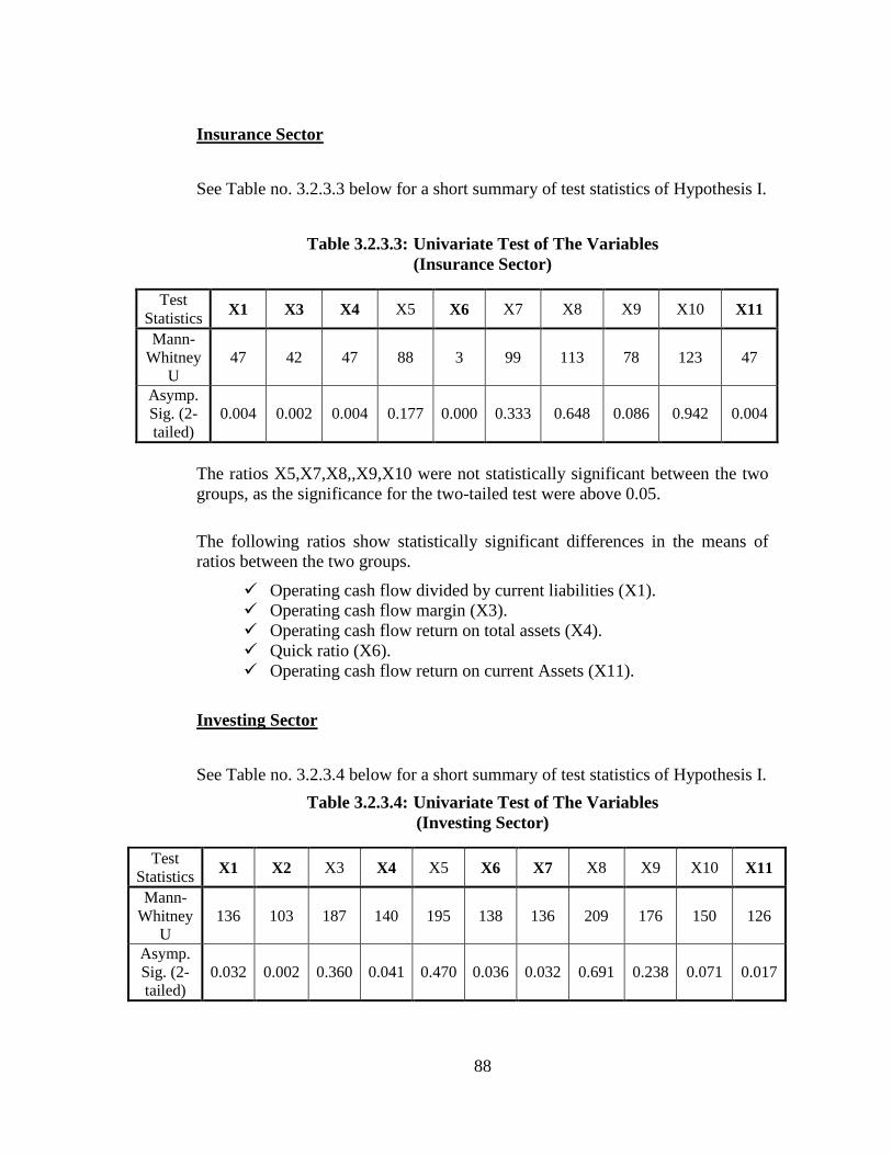
88
Insurance Sector
See Table no. 3.2.3.3 below for a short summary of test statistics of Hypothesis I.
Table 3.2.3.3: Univariate Test of The Variables
(Insurance Sector)
Test
Statistics X1 X3 X4 X5 X6 X7 X8 X9 X10 X11
Mann-
Whitney
U
47 42 47 88 3 99 113 78 123 47
Asymp.
Sig. (2-
tailed)
0.004 0.002 0.004 0.177 0.000 0.333 0.648 0.086 0.942 0.004
The ratios X5,X7,X8,,X9,X10 were not statistically significant between the two
groups, as the significance for the two-tailed test were above 0.05.
The following ratios show statistically significant differences in the means of
ratios between the two groups.
Operating cash flow divided by current liabilities (X1).
Operating cash flow margin (X3).
Operating cash flow return on total assets (X4).
Quick ratio (X6).
Operating cash flow return on current Assets (X11).
Investing Sector
See Table no. 3.2.3.4 below for a short summary of test statistics of Hypothesis I.
Table 3.2.3.4: Univariate Test of The Variables
(Investing Sector)
Test
Statistics X1 X2 X3 X4 X5 X6 X7 X8 X9 X10 X11
Mann-
Whitney
U
136 103 187 140 195 138 136 209 176 150 126
Asymp.
Sig. (2-
tailed)
0.032 0.002 0.360 0.041 0.470 0.036 0.032 0.691 0.238 0.071 0.017
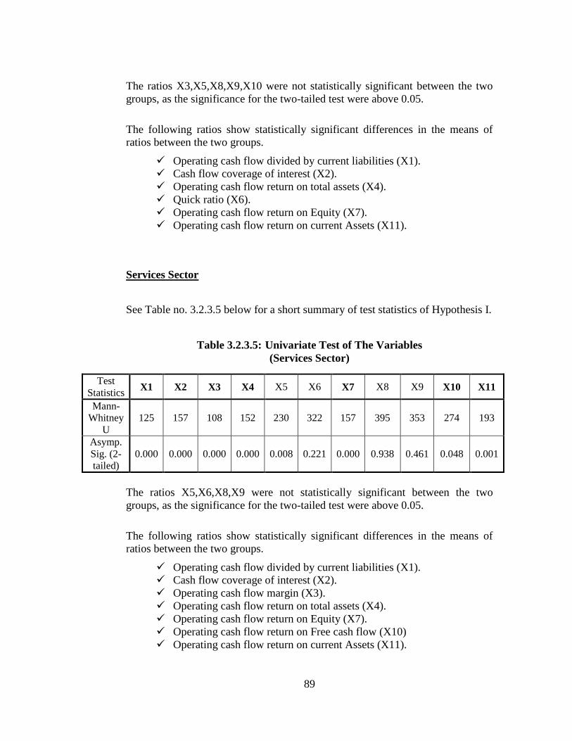
89
The ratios X3,X5,X8,X9,X10 were not statistically significant between the two
groups, as the significance for the two-tailed test were above 0.05.
The following ratios show statistically significant differences in the means of
ratios between the two groups.
Operating cash flow divided by current liabilities (X1).
Cash flow coverage of interest (X2).
Operating cash flow return on total assets (X4).
Quick ratio (X6).
Operating cash flow return on Equity (X7).
Operating cash flow return on current Assets (X11).
Services Sector
See Table no. 3.2.3.5 below for a short summary of test statistics of Hypothesis I.
Table 3.2.3.5: Univariate Test of The Variables
(Services Sector)
Test
Statistics X1 X2 X3 X4 X5 X6 X7 X8 X9 X10 X11
Mann-
Whitney
U
125 157 108 152 230 322 157 395 353 274 193
Asymp.
Sig. (2-
tailed)
0.000 0.000 0.000 0.000 0.008 0.221 0.000 0.938 0.461 0.048 0.001
The ratios X5,X6,X8,X9 were not statistically significant between the two
groups, as the significance for the two-tailed test were above 0.05.
The following ratios show statistically significant differences in the means of
ratios between the two groups.
Operating cash flow divided by current liabilities (X1).
Cash flow coverage of interest (X2).
Operating cash flow margin (X3).
Operating cash flow return on total assets (X4).
Operating cash flow return on Equity (X7).
Operating cash flow return on Free cash flow (X10)
Operating cash flow return on current Assets (X11).
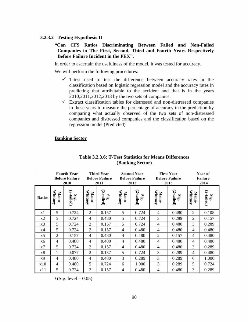
90
3.2.3.2 Testing Hypothesis II
“Can CFS Ratios Discriminating Between Failed and Non-Failed
Companies in The First, Second, Third and Fourth Years Respectively
Before Failure Incident in the PEX”.
In order to ascertain the usefulness of the model, it was tested for accuracy.
We will perform the following procedures:
T-test used to test the difference between accuracy rates in the
classification based on logistic regression model and the accuracy rates in
predicting that attributable to the accident and that is in the years
2010,2011,2012,2013 by the two sets of companies.
Extract classification tables for distressed and non-distressed companies
in these years to measure the percentage of accuracy in the prediction by
comparing what actually observed of the two sets of non-distressed
companies and distressed companies and the classification based on the
regression model (Predicted).
Banking Sector
Table 3.2.3.6: T-Test Statistics for Means Differences
(Banking Sector)
Fourth Year
Before Failure
2010
Third Year
Before Failure
2011
Second Year
Before Failure
2012
First Year
Before Failure
2013
Year of
Failure
2014
Ratios
Ma
nn
-
Wh
itney
Sig
.
(2-ta
iled)
Ma
nn
-
Wh
itney
Sig
.
(2-ta
iled)
Ma
nn
-
Wh
itney
Sig
.
(2-ta
iled)
Ma
nn
-
Wh
itney
Sig
.
(2-ta
iled)
Ma
nn
-
Wh
itney
Sig
.
(2-ta
iled)
x1 5 0.724 2 0.157 5 0.724 4 0.480 2 0.108
x2 5 0.724 4 0.480 5 0.724 3 0.289 2 0.157
x3 5 0.724 2 0.157 5 0.724 4 0.480 3 0.289
x4 5 0.724 2 0.157 4 0.480 4 0.480 4 0.480
x5 2 0.157 4 0.480 4 0.480 2 0.157 4 0.480
x6 4 0.480 4 0.480 4 0.480 4 0.480 4 0.480
x7 5 0.724 2 0.157 4 0.480 4 0.480 3 0.289
x8 1 0.077 2 0.157 5 0.724 3 0.289 4 0.480
x9 4 0.480 4 0.480 3 0.289 3 0.289 6 1.000
x10 4 0.480 5 0.724 6 1.000 3 0.289 5 0.724
x11 5 0.724 2 0.157 4 0.480 4 0.480 3 0.289
(Sig. level = 0.05)
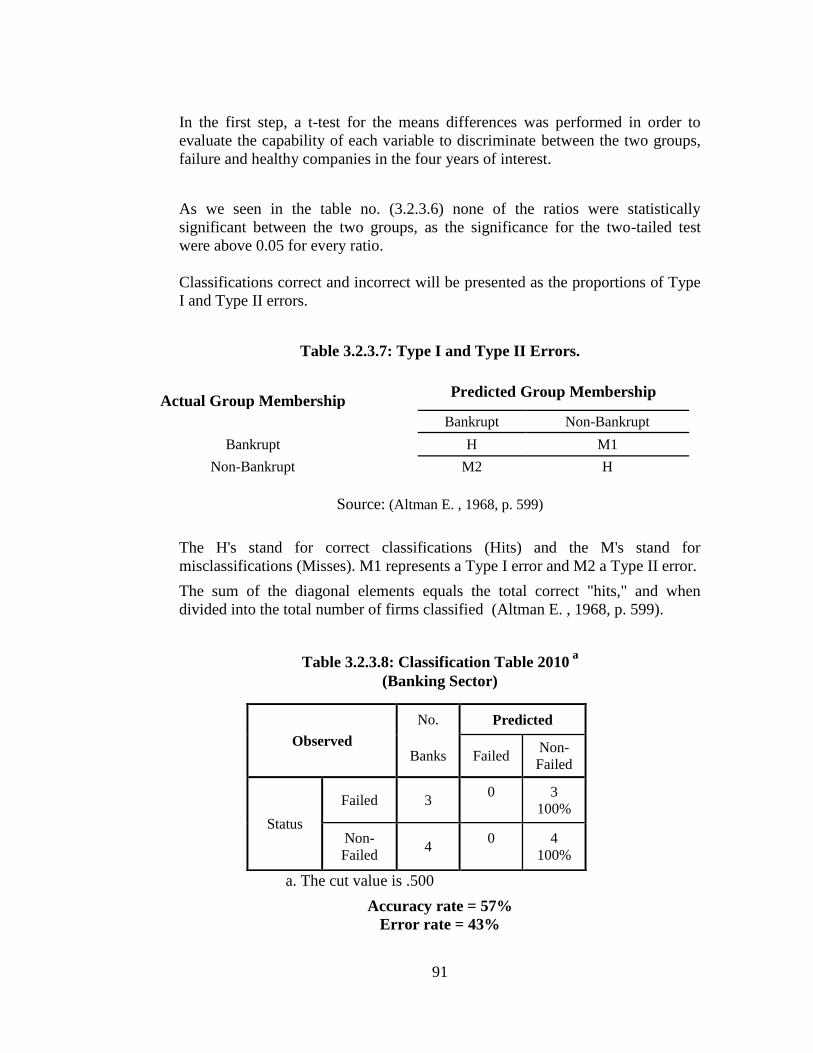
91
In the first step, a t-test for the means differences was performed in order to
evaluate the capability of each variable to discriminate between the two groups,
failure and healthy companies in the four years of interest.
As we seen in the table no. (3.2.3.6) none of the ratios were statistically
significant between the two groups, as the significance for the two-tailed test
were above 0.05 for every ratio.
Classifications correct and incorrect will be presented as the proportions of Type
I and Type II errors.
Table 3.2.3.7: Type I and Type II Errors.
Actual Group Membership Predicted Group Membership
Bankrupt Non-Bankrupt
Bankrupt
H M1
Non-Bankrupt
M2 H
Source: (Altman E. , 1968, p. 599)
The H's stand for correct classifications (Hits) and the M's stand for
misclassifications (Misses). M1 represents a Type I error and M2 a Type II error.
The sum of the diagonal elements equals the total correct "hits," and when
divided into the total number of firms classified (Altman E. , 1968, p. 599).
Table 3.2.3.8: Classification Table 2010 a
(Banking Sector)
a. The cut value is .500
Accuracy rate = 57%
Error rate = 43%
Observed
No. Predicted
Banks Failed Non-
Failed
Status
Failed 3 0
3
100%
Non-
Failed 4
0
4
100%
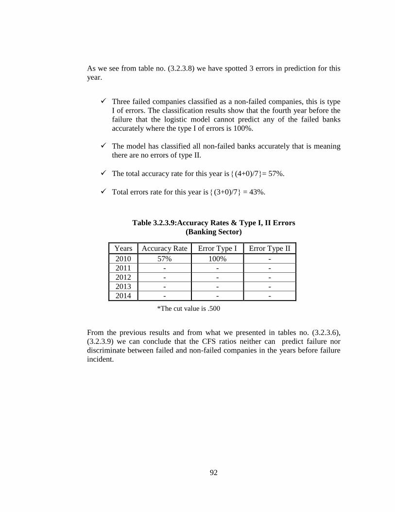
92
As we see from table no. (3.2.3.8) we have spotted 3 errors in prediction for this
year.
Three failed companies classified as a non-failed companies, this is type
I of errors. The classification results show that the fourth year before the
failure that the logistic model cannot predict any of the failed banks
accurately where the type I of errors is 100%.
The model has classified all non-failed banks accurately that is meaning
there are no errors of type II.
The total accuracy rate for this year is (4+0)/7= 57%.
Total errors rate for this year is (3+0)/7 = 43%.
Table 3.2.3.9:Accuracy Rates & Type I, II Errors
(Banking Sector)
Years Accuracy Rate Error Type I Error Type II
2010 57% 100% -
2011 - - -
2012 - - -
2013 - - -
2014 - - -
*The cut value is .500
From the previous results and from what we presented in tables no. (3.2.3.6),
(3.2.3.9) we can conclude that the CFS ratios neither can predict failure nor
discriminate between failed and non-failed companies in the years before failure
incident.
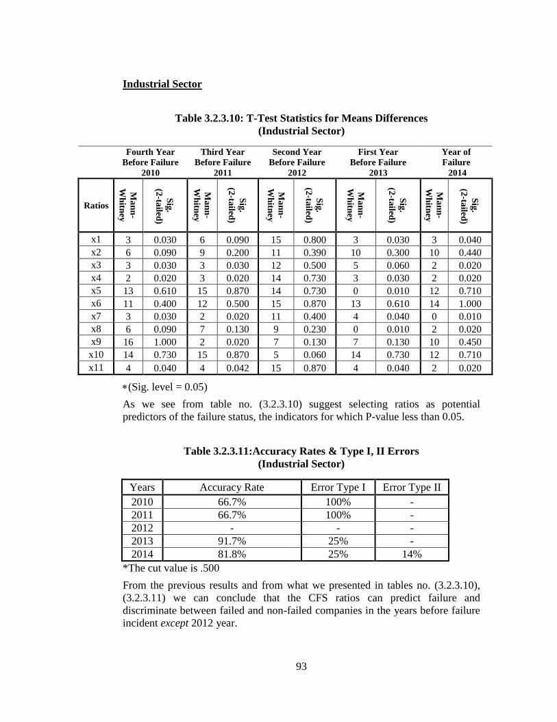
93
Industrial Sector
Table 3.2.3.10: T-Test Statistics for Means Differences
(Industrial Sector)
Fourth Year
Before Failure
2010
Third Year
Before Failure
2011
Second Year
Before Failure
2012
First Year
Before Failure
2013
Year of
Failure
2014
Ratios
Ma
nn
-
Wh
itney
Sig
.
(2-ta
iled)
Ma
nn
-
Wh
itney
Sig
.
(2-ta
iled)
Ma
nn
-
Wh
itney
Sig
.
(2-ta
iled)
Ma
nn
-
Wh
itney
Sig
.
(2-ta
iled)
Ma
nn
-
Wh
itney
Sig
.
(2-ta
iled)
x1 3 0.030 6 0.090 15 0.800 3 0.030 3 0.040
x2 6 0.090 9 0.200 11 0.390 10 0.300 10 0.440
x3 3 0.030 3 0.030 12 0.500 5 0.060 2 0.020
x4 2 0.020 3 0.020 14 0.730 3 0.030 2 0.020
x5 13 0.610 15 0.870 14 0.730 0 0.010 12 0.710
x6 11 0.400 12 0.500 15 0.870 13 0.610 14 1.000
x7 3 0.030 2 0.020 11 0.400 4 0.040 0 0.010
x8 6 0.090 7 0.130 9 0.230 0 0.010 2 0.020
x9 16 1.000 2 0.020 7 0.130 7 0.130 10 0.450
x10 14 0.730 15 0.870 5 0.060 14 0.730 12 0.710
x11 4 0.040 4 0.042 15 0.870 4 0.040 2 0.020
(Sig. level = 0.05)
As we see from table no. (3.2.3.10) suggest selecting ratios as potential
predictors of the failure status, the indicators for which P-value less than 0.05.
Table 3.2.3.11:Accuracy Rates & Type I, II Errors
(Industrial Sector)
Years Accuracy Rate Error Type I Error Type II
2010 66.7% 100% -
2011 66.7% 100% -
2012 - - -
2013 91.7% 25% -
2014 81.8% 25% 14%
*The cut value is .500
From the previous results and from what we presented in tables no. (3.2.3.10),
(3.2.3.11) we can conclude that the CFS ratios can predict failure and
discriminate between failed and non-failed companies in the years before failure
incident except 2012 year.
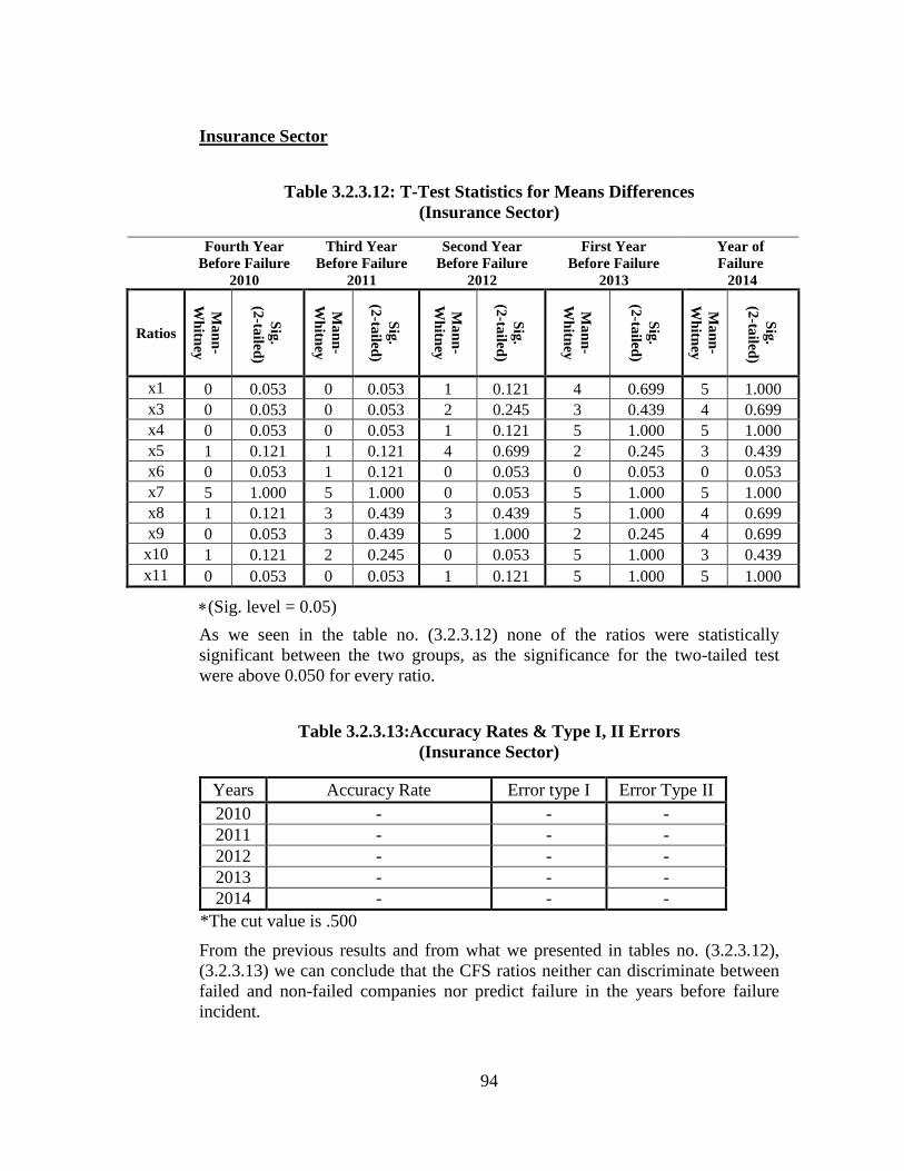
94
Insurance Sector
Table 3.2.3.12: T-Test Statistics for Means Differences
(Insurance Sector)
Fourth Year
Before Failure
2010
Third Year
Before Failure
2011
Second Year
Before Failure
2012
First Year
Before Failure
2013
Year of
Failure
2014
Ratios
Ma
nn
-
Wh
itney
Sig
.
(2-ta
iled)
Ma
nn
-
Wh
itney
Sig
.
(2-ta
iled)
Ma
nn
-
Wh
itney
Sig
.
(2-ta
iled)
Ma
nn
-
Wh
itney
Sig
.
(2-ta
iled)
Ma
nn
-
Wh
itney
Sig
.
(2-ta
iled)
x1 0 0.053 0 0.053 1 0.121 4 0.699 5 1.000
x3 0 0.053 0 0.053 2 0.245 3 0.439 4 0.699
x4 0 0.053 0 0.053 1 0.121 5 1.000 5 1.000
x5 1 0.121 1 0.121 4 0.699 2 0.245 3 0.439
x6 0 0.053 1 0.121 0 0.053 0 0.053 0 0.053
x7 5 1.000 5 1.000 0 0.053 5 1.000 5 1.000
x8 1 0.121 3 0.439 3 0.439 5 1.000 4 0.699
x9 0 0.053 3 0.439 5 1.000 2 0.245 4 0.699
x10 1 0.121 2 0.245 0 0.053 5 1.000 3 0.439
x11 0 0.053 0 0.053 1 0.121 5 1.000 5 1.000
(Sig. level = 0.05)
As we seen in the table no. (3.2.3.12) none of the ratios were statistically
significant between the two groups, as the significance for the two-tailed test
were above 0.050 for every ratio.
Table 3.2.3.13:Accuracy Rates & Type I, II Errors
(Insurance Sector)
Years Accuracy Rate Error type I Error Type II
2010 - - -
2011 - - -
2012 - - -
2013 - - -
2014 - - -
*The cut value is .500
From the previous results and from what we presented in tables no. (3.2.3.12),
(3.2.3.13) we can conclude that the CFS ratios neither can discriminate between
failed and non-failed companies nor predict failure in the years before failure
incident.
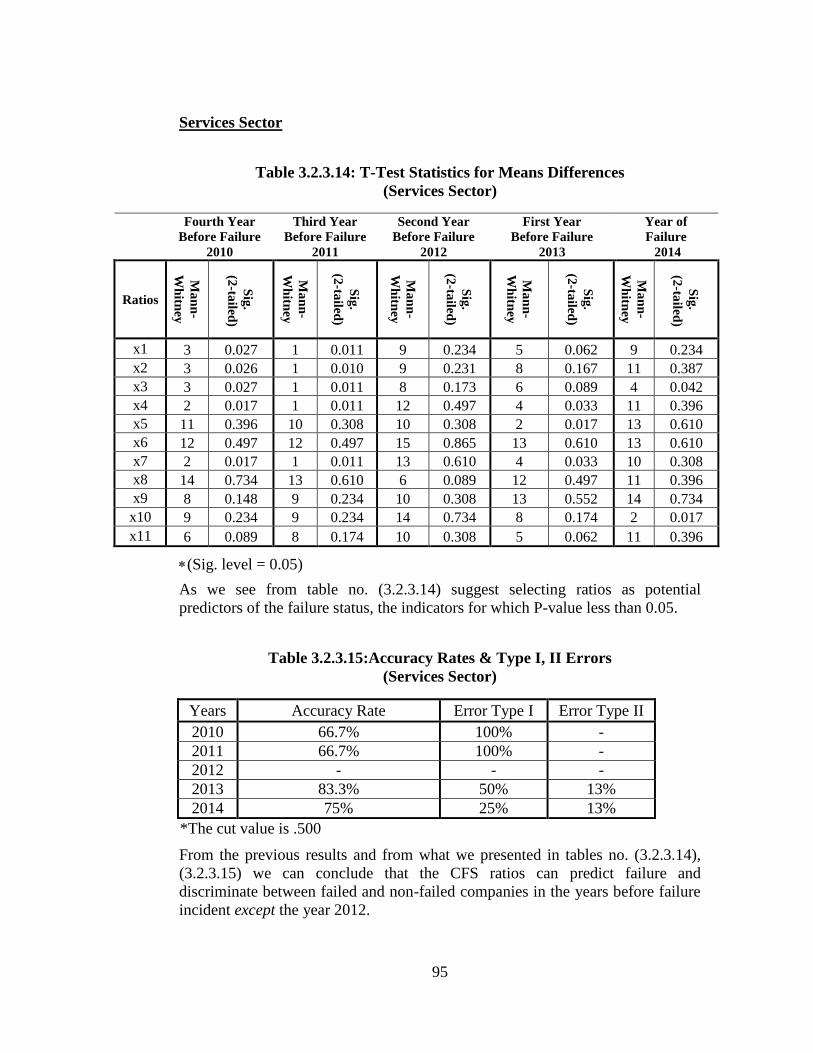
95
Services Sector
Table 3.2.3.14: T-Test Statistics for Means Differences
(Services Sector)
Fourth Year
Before Failure
2010
Third Year
Before Failure
2011
Second Year
Before Failure
2012
First Year
Before Failure
2013
Year of
Failure
2014
Ratios
Ma
nn
-
Wh
itney
Sig
.
(2-ta
iled)
Ma
nn
-
Wh
itney
Sig
.
(2-ta
iled)
Ma
nn
-
Wh
itney
Sig
.
(2-ta
iled)
Ma
nn
-
Wh
itney
Sig
.
(2-ta
iled)
Ma
nn
-
Wh
itney
Sig
.
(2-ta
iled)
x1 3 0.027 1 0.011 9 0.234 5 0.062 9 0.234
x2 3 0.026 1 0.010 9 0.231 8 0.167 11 0.387
x3 3 0.027 1 0.011 8 0.173 6 0.089 4 0.042
x4 2 0.017 1 0.011 12 0.497 4 0.033 11 0.396
x5 11 0.396 10 0.308 10 0.308 2 0.017 13 0.610
x6 12 0.497 12 0.497 15 0.865 13 0.610 13 0.610
x7 2 0.017 1 0.011 13 0.610 4 0.033 10 0.308
x8 14 0.734 13 0.610 6 0.089 12 0.497 11 0.396
x9 8 0.148 9 0.234 10 0.308 13 0.552 14 0.734
x10 9 0.234 9 0.234 14 0.734 8 0.174 2 0.017
x11 6 0.089 8 0.174 10 0.308 5 0.062 11 0.396
(Sig. level = 0.05)
As we see from table no. (3.2.3.14) suggest selecting ratios as potential
predictors of the failure status, the indicators for which P-value less than 0.05.
Table 3.2.3.15:Accuracy Rates & Type I, II Errors
(Services Sector)
Years Accuracy Rate Error Type I Error Type II
2010 66.7% 100% -
2011 66.7% 100% -
2012 - - -
2013 83.3% 50% 13%
2014 75% 25% 13%
*The cut value is .500
From the previous results and from what we presented in tables no. (3.2.3.14),
(3.2.3.15) we can conclude that the CFS ratios can predict failure and
discriminate between failed and non-failed companies in the years before failure
incident except the year 2012.
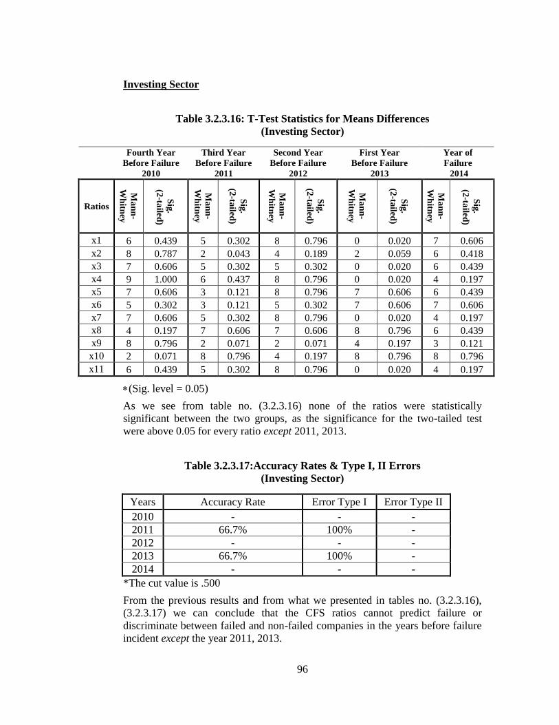
96
Investing Sector
Table 3.2.3.16: T-Test Statistics for Means Differences
(Investing Sector)
Fourth Year
Before Failure
2010
Third Year
Before Failure
2011
Second Year
Before Failure
2012
First Year
Before Failure
2013
Year of
Failure
2014
Ratios
Ma
nn
-
Wh
itney
Sig
.
(2-ta
iled)
Ma
nn
-
Wh
itney
Sig
.
(2-ta
iled)
Ma
nn
-
Wh
itney
Sig
.
(2-ta
iled)
Ma
nn
-
Wh
itney
Sig
.
(2-ta
iled)
Ma
nn
-
Wh
itney
Sig
.
(2-ta
iled)
x1 6 0.439 5 0.302 8 0.796 0 0.020 7 0.606
x2 8 0.787 2 0.043 4 0.189 2 0.059 6 0.418
x3 7 0.606 5 0.302 5 0.302 0 0.020 6 0.439
x4 9 1.000 6 0.437 8 0.796 0 0.020 4 0.197
x5 7 0.606 3 0.121 8 0.796 7 0.606 6 0.439
x6 5 0.302 3 0.121 5 0.302 7 0.606 7 0.606
x7 7 0.606 5 0.302 8 0.796 0 0.020 4 0.197
x8 4 0.197 7 0.606 7 0.606 8 0.796 6 0.439
x9 8 0.796 2 0.071 2 0.071 4 0.197 3 0.121
x10 2 0.071 8 0.796 4 0.197 8 0.796 8 0.796
x11 6 0.439 5 0.302 8 0.796 0 0.020 4 0.197
(Sig. level = 0.05)
As we see from table no. (3.2.3.16) none of the ratios were statistically
significant between the two groups, as the significance for the two-tailed test
were above 0.05 for every ratio except 2011, 2013.
Table 3.2.3.17:Accuracy Rates & Type I, II Errors
(Investing Sector)
Years Accuracy Rate Error Type I Error Type II
2010 - - -
2011 66.7% 100% -
2012 - - -
2013 66.7% 100% -
2014 - - -
*The cut value is .500
From the previous results and from what we presented in tables no. (3.2.3.16),
(3.2.3.17) we can conclude that the CFS ratios cannot predict failure or
discriminate between failed and non-failed companies in the years before failure
incident except the year 2011, 2013.
97
3.2.3.3 Testing Hypothesis III
“The Following Financial Ratios in The Proposed Developed Model Can
Predict Financial Failure in the PEX”.
Operating cash flow on current liabilities (OCF/CL).
Cash flow coverage of interest (OCF + INTREST + TAX/INT).
Operating cash flow margin (OCF/Sales).
Operating cash flow return on total assets (OCF/Asset).
Earning quality (EBIT/OCF).
Quick ratio or acid-test ratio (CA-INV)/CL.
Operating Cash flow on Equity (OCF/EQUITY).
Operating Cash flow on Net Income (OCF/N.I).
Operating Cash flow on Current Assets (OCF/C.A).
Free Cash Flow on Current Liabilities (FCF/C.L).
Operating Cash flow on Free Cash Flow (OCF/FCF).
―Logistic regression is an attractive alternative to discriminant analysis. Its
empirical results parallel those of multiple regression in terms of their
interpretation and the casewise diagnostic measures available for examining
residuals and it handles categorical independent variable easily whereas in
discriminant analysis the use of dummy variables created problems with the
variance covariance equalities. Logistic regression requires less restrictive
statistical assumptions so the use of logit analysis essentially avoids all of the
problems discussed with respect to discriminant analysis. Even if the
assumptions are met, many researchers prefer logistic regression because it is
similar to multiple regression. It has straightforward statistical tests, similar
approaches to incorporating metric and nonmetric‖ (Vuran, 2009, p. 55).
The univariate analysis (t-test) provides evidence of those variables to be
considered as candidates for model building. However, in a multivariate setting it
may be the case that a collective set of variables might achieve a better degree of
discrimination power between the two groups of firms. Therefore, in order to
avoid potential bias and improve the overall performance, we supplemented our
model development process with further variable selection techniques. Starting
from the previous results, we use the stepwise method to determine the final set
of variables to be included in the discrimination model. In particular we refer to a
step-by-step backward selection. The procedure begins with all variables in the
model and at each step the weight of each variable is evaluated to determine
which one will contribute most to the discriminatory power of the model.
Logistic Regression analyses are conducted with the representative ratios using
SPSS software. To select the best set of discriminating ratios stepwise selection
criteria is applied. The empirical results are explained later for each sector of the
study.
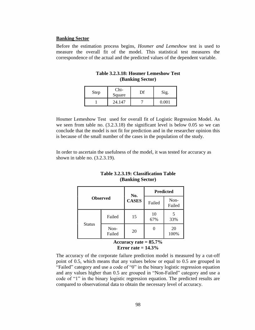
98
Banking Sector
Before the estimation process begins, Hosmer and Lemeshow test is used to
measure the overall fit of the model. This statistical test measures the
correspondence of the actual and the predicted values of the dependent variable.
Table 3.2.3.18: Hosmer Lemeshow Test
(Banking Sector)
Step Chi-
Square Df Sig.
1 24.147 7 0.001
Hosmer Lemeshow Test used for overall fit of Logistic Regression Model. As
we seen from table no. (3.2.3.18) the significant level is below 0.05 so we can
conclude that the model is not fit for prediction and in the researcher opinion this
is because of the small number of the cases in the population of the study.
In order to ascertain the usefulness of the model, it was tested for accuracy as
shown in table no. (3.2.3.19).
Table 3.2.3.19: Classification Table
(Banking Sector)
Accuracy rate = 85.7%
Error rate = 14.3%
The accuracy of the corporate failure prediction model is measured by a cut-off
point of 0.5, which means that any values below or equal to 0.5 are grouped in
―Failed‖ category and use a code of ―0‖ in the binary logistic regression equation
and any values higher than 0.5 are grouped in ―Non-Failed‖ category and use a
code of ―1‖ in the binary logistic regression equation. The predicted results are
compared to observational data to obtain the necessary level of accuracy.
Observed No.
CASES
Predicted
Failed Non-
Failed
Status
Failed 15 10
67%
5
33%
Non-
Failed 20
0
20
100%
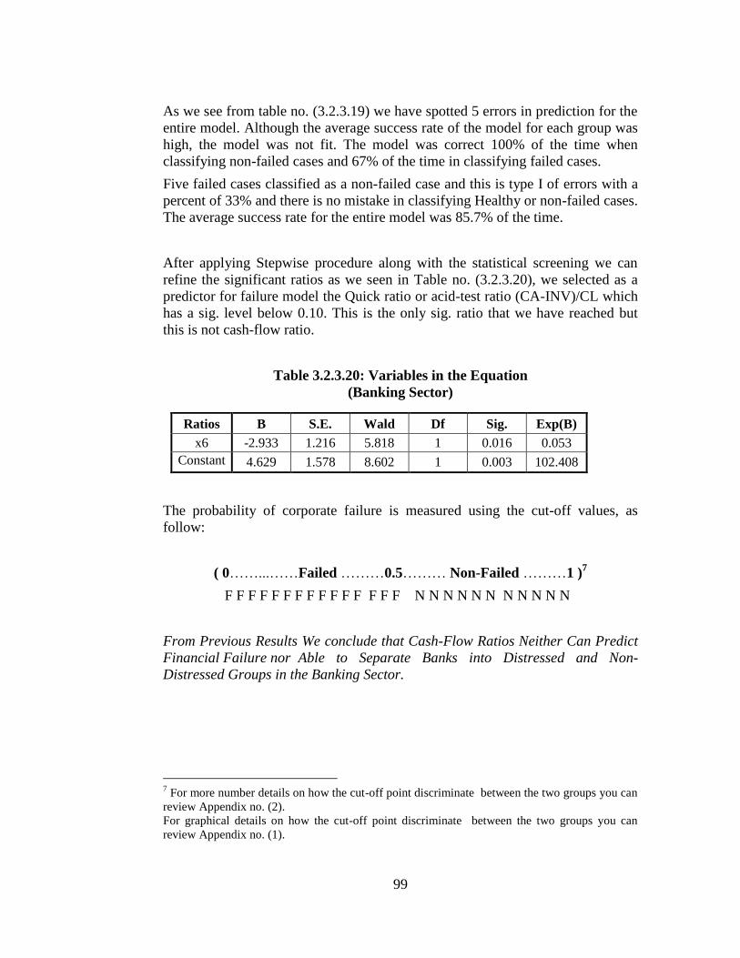
99
As we see from table no. (3.2.3.19) we have spotted 5 errors in prediction for the
entire model. Although the average success rate of the model for each group was
high, the model was not fit. The model was correct 100% of the time when
classifying non-failed cases and 67% of the time in classifying failed cases.
Five failed cases classified as a non-failed case and this is type I of errors with a
percent of 33% and there is no mistake in classifying Healthy or non-failed cases.
The average success rate for the entire model was 85.7% of the time.
After applying Stepwise procedure along with the statistical screening we can
refine the significant ratios as we seen in Table no. (3.2.3.20), we selected as a
predictor for failure model the Quick ratio or acid-test ratio (CA-INV)/CL which
has a sig. level below 0.10. This is the only sig. ratio that we have reached but
this is not cash-flow ratio.
Table 3.2.3.20: Variables in the Equation
(Banking Sector)
Ratios B S.E. Wald Df Sig. Exp(B)
x6 -2.933 1.216 5.818 1 0.016 0.053
Constant 4.629 1.578 8.602 1 0.003 102.408
The probability of corporate failure is measured using the cut-off values, as
follow:
( 0……...……Failed ………0.5……… Non-Failed ………1 )7
F F F F F F F F F F F F F F F N N N N N N N N N N N
From Previous Results We conclude that Cash-Flow Ratios Neither Can Predict
Financial Failure nor Able to Separate Banks into Distressed and Non-
Distressed Groups in the Banking Sector.
7 For more number details on how the cut-off point discriminate between the two groups you can
review Appendix no. (2).
For graphical details on how the cut-off point discriminate between the two groups you can
review Appendix no. (1).
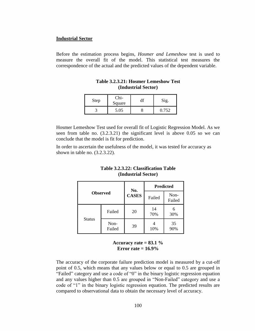
100
Industrial Sector
Before the estimation process begins, Hosmer and Lemeshow test is used to
measure the overall fit of the model. This statistical test measures the
correspondence of the actual and the predicted values of the dependent variable.
Table 3.2.3.21: Hosmer Lemeshow Test
(Industrial Sector)
Step Chi-
Square df Sig.
3 5.05 8 0.752
Hosmer Lemeshow Test used for overall fit of Logistic Regression Model. As we
seen from table no. (3.2.3.21) the significant level is above 0.05 so we can
conclude that the model is fit for prediction.
In order to ascertain the usefulness of the model, it was tested for accuracy as
shown in table no. (3.2.3.22).
Table 3.2.3.22: Classification Table
(Industrial Sector)
Accuracy rate = 83.1 %
Error rate = 16.9%
The accuracy of the corporate failure prediction model is measured by a cut-off
point of 0.5, which means that any values below or equal to 0.5 are grouped in
―Failed‖ category and use a code of ―0‖ in the binary logistic regression equation
and any values higher than 0.5 are grouped in ―Non-Failed‖ category and use a
code of ―1‖ in the binary logistic regression equation. The predicted results are
compared to observational data to obtain the necessary level of accuracy.
Observed No.
CASES
Predicted
Failed Non-
Failed
Status
Failed 20 14
70%
6
30%
Non-
Failed 39
4
10%
35
90%
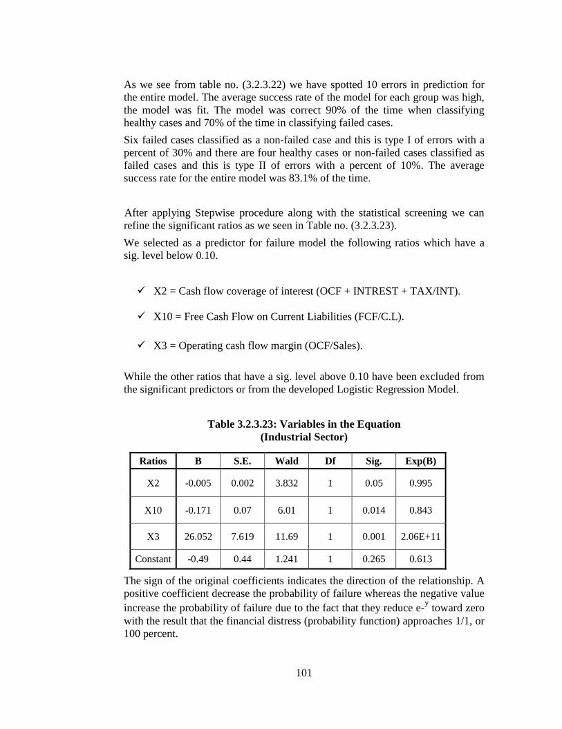
101
As we see from table no. (3.2.3.22) we have spotted 10 errors in prediction for
the entire model. The average success rate of the model for each group was high,
the model was fit. The model was correct 90% of the time when classifying
healthy cases and 70% of the time in classifying failed cases.
Six failed cases classified as a non-failed case and this is type I of errors with a
percent of 30% and there are four healthy cases or non-failed cases classified as
failed cases and this is type II of errors with a percent of 10%. The average
success rate for the entire model was 83.1% of the time.
After applying Stepwise procedure along with the statistical screening we can
refine the significant ratios as we seen in Table no. (3.2.3.23).
We selected as a predictor for failure model the following ratios which have a
sig. level below 0.10.
X2 = Cash flow coverage of interest (OCF + INTREST + TAX/INT).
X10 = Free Cash Flow on Current Liabilities (FCF/C.L).
X3 = Operating cash flow margin (OCF/Sales).
While the other ratios that have a sig. level above 0.10 have been excluded from
the significant predictors or from the developed Logistic Regression Model.
Table 3.2.3.23: Variables in the Equation
(Industrial Sector)
Ratios B S.E. Wald Df Sig. Exp(B)
X2 -0.005 0.002 3.832 1 0.05 0.995
X10 -0.171 0.07 6.01 1 0.014 0.843
X3 26.052 7.619 11.69 1 0.001 2.06E+11
Constant -0.49 0.44 1.241 1 0.265 0.613
The sign of the original coefficients indicates the direction of the relationship. A
positive coefficient decrease the probability of failure whereas the negative value
increase the probability of failure due to the fact that they reduce e-y toward zero
with the result that the financial distress (probability function) approaches 1/1, or
100 percent.
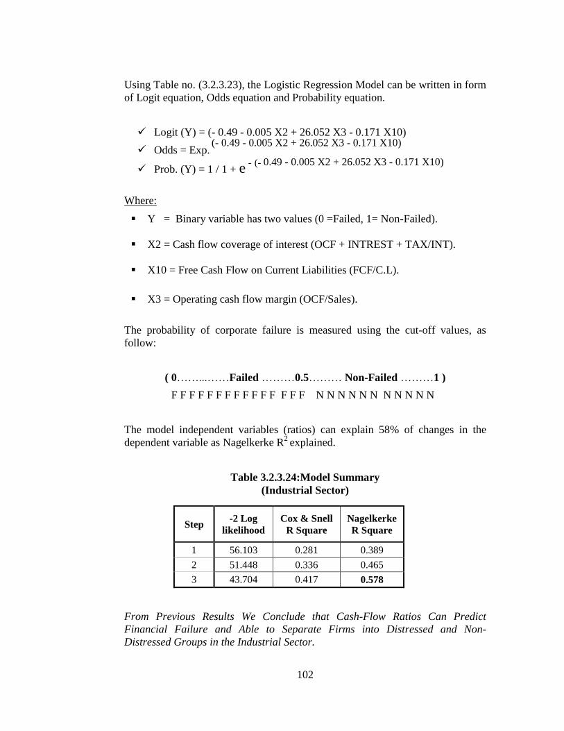
102
Using Table no. (3.2.3.23), the Logistic Regression Model can be written in form
of Logit equation, Odds equation and Probability equation.
Logit (Y) = (- 0.49 - 0.005 X2 + 26.052 X3 - 0.171 X10)
Odds = Exp. (- 0.49 - 0.005 X2 + 26.052 X3 - 0.171 X10)
Prob. (Y) = 1 / 1 + e - (- 0.49 - 0.005 X2 + 26.052 X3 - 0.171 X10)
Where:
Y = Binary variable has two values (0 =Failed, 1= Non-Failed).
X2 = Cash flow coverage of interest (OCF + INTREST + TAX/INT).
X10 = Free Cash Flow on Current Liabilities (FCF/C.L).
X3 = Operating cash flow margin (OCF/Sales).
The probability of corporate failure is measured using the cut-off values, as
follow:
( 0……...……Failed ………0.5……… Non-Failed ………1 )
F F F F F F F F F F F F F F F N N N N N N N N N N N
The model independent variables (ratios) can explain 58% of changes in the
dependent variable as Nagelkerke R2
explained.
Table 3.2.3.24:Model Summary
(Industrial Sector)
Step -2 Log
likelihood
Cox & Snell
R Square
Nagelkerke
R Square
1 56.103 0.281 0.389
2 51.448 0.336 0.465
3 43.704 0.417 0.578
From Previous Results We Conclude that Cash-Flow Ratios Can Predict
Financial Failure and Able to Separate Firms into Distressed and Non-
Distressed Groups in the Industrial Sector.
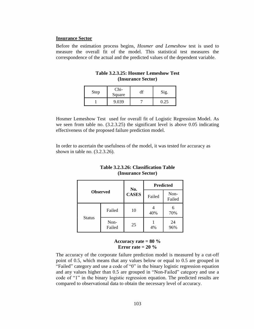
103
Insurance Sector
Before the estimation process begins, Hosmer and Lemeshow test is used to
measure the overall fit of the model. This statistical test measures the
correspondence of the actual and the predicted values of the dependent variable.
Table 3.2.3.25: Hosmer Lemeshow Test
(Insurance Sector)
Step Chi-
Square df Sig.
1 9.039 7 0.25
Hosmer Lemeshow Test used for overall fit of Logistic Regression Model. As
we seen from table no. (3.2.3.25) the significant level is above 0.05 indicating
effectiveness of the proposed failure prediction model.
In order to ascertain the usefulness of the model, it was tested for accuracy as
shown in table no. (3.2.3.26).
Table 3.2.3.26: Classification Table
(Insurance Sector)
Accuracy rate = 80 %
Error rate = 20 %
The accuracy of the corporate failure prediction model is measured by a cut-off
point of 0.5, which means that any values below or equal to 0.5 are grouped in
―Failed‖ category and use a code of ―0‖ in the binary logistic regression equation
and any values higher than 0.5 are grouped in ―Non-Failed‖ category and use a
code of ―1‖ in the binary logistic regression equation. The predicted results are
compared to observational data to obtain the necessary level of accuracy.
Observed No.
CASES
Predicted
Failed Non-
Failed
Status
Failed 10 4
40%
6
70%
Non-
Failed 25
1
4%
24
96%
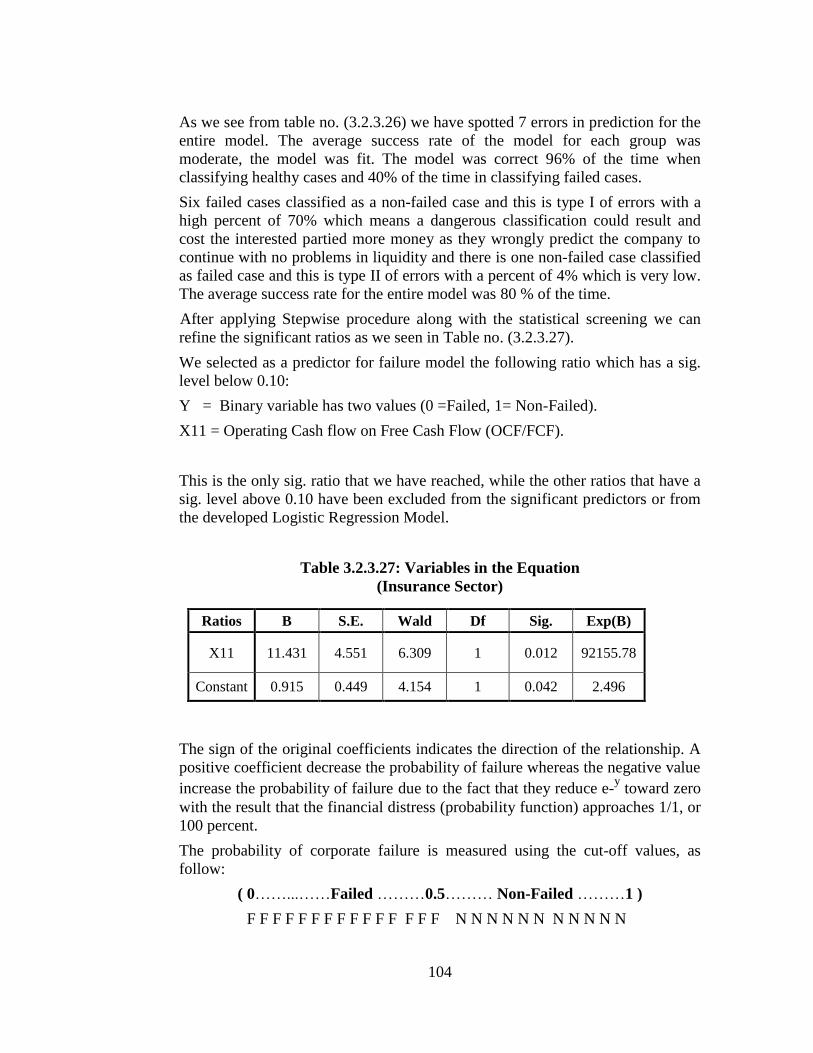
104
As we see from table no. (3.2.3.26) we have spotted 7 errors in prediction for the
entire model. The average success rate of the model for each group was
moderate, the model was fit. The model was correct 96% of the time when
classifying healthy cases and 40% of the time in classifying failed cases.
Six failed cases classified as a non-failed case and this is type I of errors with a
high percent of 70% which means a dangerous classification could result and
cost the interested partied more money as they wrongly predict the company to
continue with no problems in liquidity and there is one non-failed case classified
as failed case and this is type II of errors with a percent of 4% which is very low.
The average success rate for the entire model was 80 % of the time.
After applying Stepwise procedure along with the statistical screening we can
refine the significant ratios as we seen in Table no. (3.2.3.27).
We selected as a predictor for failure model the following ratio which has a sig.
level below 0.10:
Y = Binary variable has two values (0 =Failed, 1= Non-Failed).
X11 = Operating Cash flow on Free Cash Flow (OCF/FCF).
This is the only sig. ratio that we have reached, while the other ratios that have a
sig. level above 0.10 have been excluded from the significant predictors or from
the developed Logistic Regression Model.
Table 3.2.3.27: Variables in the Equation
(Insurance Sector)
Ratios B S.E. Wald Df Sig. Exp(B)
X11 11.431 4.551 6.309 1 0.012 92155.78
Constant 0.915 0.449 4.154 1 0.042 2.496
The sign of the original coefficients indicates the direction of the relationship. A
positive coefficient decrease the probability of failure whereas the negative value
increase the probability of failure due to the fact that they reduce e-y toward zero
with the result that the financial distress (probability function) approaches 1/1, or
100 percent.
The probability of corporate failure is measured using the cut-off values, as
follow:
( 0……...……Failed ………0.5……… Non-Failed ………1 )
F F F F F F F F F F F F F F F N N N N N N N N N N N
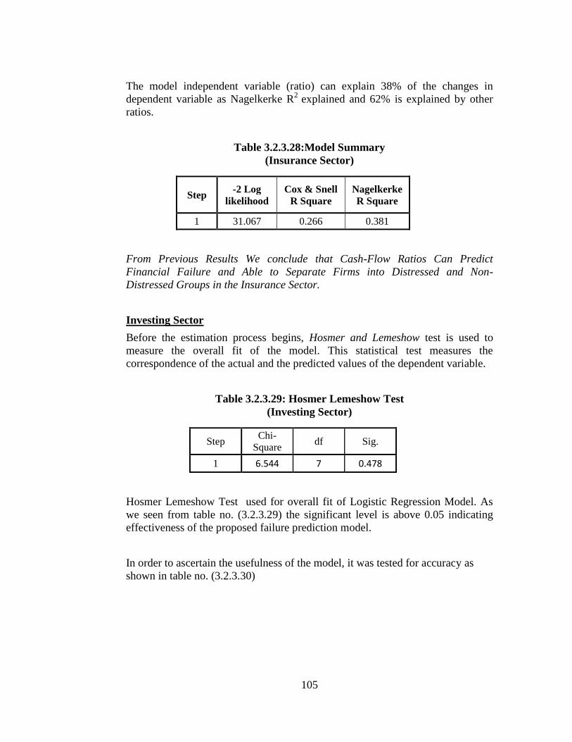
105
The model independent variable (ratio) can explain 38% of the changes in
dependent variable as Nagelkerke R2
explained and 62% is explained by other
ratios.
Table 3.2.3.28:Model Summary
(Insurance Sector)
Step -2 Log
likelihood
Cox & Snell
R Square
Nagelkerke
R Square
1 31.067 0.266 0.381
From Previous Results We conclude that Cash-Flow Ratios Can Predict
Financial Failure and Able to Separate Firms into Distressed and Non-
Distressed Groups in the Insurance Sector.
Investing Sector
Before the estimation process begins, Hosmer and Lemeshow test is used to
measure the overall fit of the model. This statistical test measures the
correspondence of the actual and the predicted values of the dependent variable.
Table 3.2.3.29: Hosmer Lemeshow Test
(Investing Sector)
Step Chi-
Square df Sig.
1 6.544 7 0.478
Hosmer Lemeshow Test used for overall fit of Logistic Regression Model. As
we seen from table no. (3.2.3.29) the significant level is above 0.05 indicating
effectiveness of the proposed failure prediction model.
In order to ascertain the usefulness of the model, it was tested for accuracy as
shown in table no. (3.2.3.30)
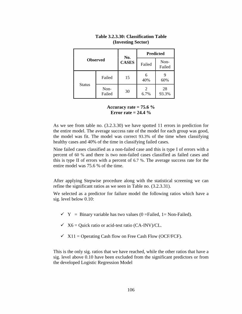
106
Table 3.2.3.30: Classification Table
(Investing Sector)
Accuracy rate = 75.6 %
Error rate = 24.4 %
As we see from table no. (3.2.3.30) we have spotted 11 errors in prediction for
the entire model. The average success rate of the model for each group was good,
the model was fit. The model was correct 93.3% of the time when classifying
healthy cases and 40% of the time in classifying failed cases.
Nine failed cases classified as a non-failed case and this is type I of errors with a
percent of 60 % and there is two non-failed cases classified as failed cases and
this is type II of errors with a percent of 6.7 %. The average success rate for the
entire model was 75.6 % of the time.
After applying Stepwise procedure along with the statistical screening we can
refine the significant ratios as we seen in Table no. (3.2.3.31).
We selected as a predictor for failure model the following ratios which have a
sig. level below 0.10:
Y = Binary variable has two values (0 =Failed, 1= Non-Failed).
X6 = Quick ratio or acid-test ratio (CA-INV)/CL.
X11 = Operating Cash flow on Free Cash Flow (OCF/FCF).
This is the only sig. ratios that we have reached, while the other ratios that have a
sig. level above 0.10 have been excluded from the significant predictors or from
the developed Logistic Regression Model
Observed No.
CASES
Predicted
Failed Non-
Failed
Status
Failed 15 6
40%
9
60%
Non-
Failed 30
2
6.7%
28
93.3%
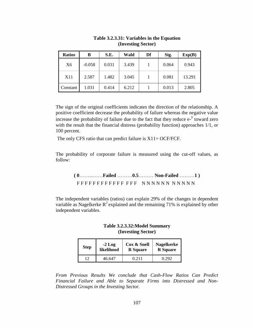
107
Table 3.2.3.31: Variables in the Equation
(Investing Sector)
Ratios B S.E. Wald Df Sig. Exp(B)
X6 -0.058 0.031 3.439 1 0.064 0.943
X11 2.587 1.482 3.045 1 0.081 13.291
Constant 1.031 0.414 6.212 1 0.013 2.805
The sign of the original coefficients indicates the direction of the relationship. A
positive coefficient decrease the probability of failure whereas the negative value
increase the probability of failure due to the fact that they reduce e-y toward zero
with the result that the financial distress (probability function) approaches 1/1, or
100 percent.
The only CFS ratio that can predict failure is X11= OCF/FCF.
The probability of corporate failure is measured using the cut-off values, as
follow:
( 0……...……Failed ………0.5……… Non-Failed ………1 )
F F F F F F F F F F F F F F F N N N N N N N N N N N
The independent variables (ratios) can explain 29% of the changes in dependent
variable as Nagelkerke R2
explained and the remaining 71% is explained by other
independent variables.
Table 3.2.3.32:Model Summary
(Investing Sector)
Step -2 Log
likelihood
Cox & Snell
R Square
Nagelkerke
R Square
12 46.647 0.211 0.292
From Previous Results We conclude that Cash-Flow Ratios Can Predict
Financial Failure and Able to Separate Firms into Distressed and Non-
Distressed Groups in the Investing Sector.
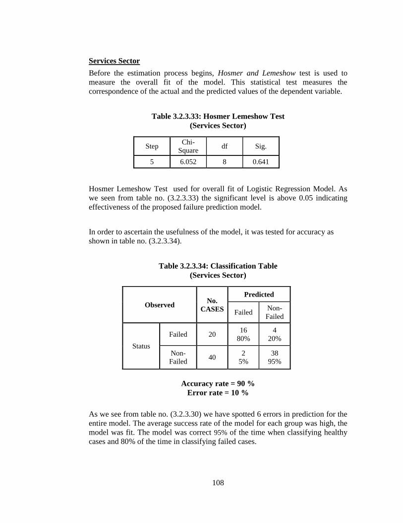
108
Services Sector
Before the estimation process begins, Hosmer and Lemeshow test is used to
measure the overall fit of the model. This statistical test measures the
correspondence of the actual and the predicted values of the dependent variable.
Table 3.2.3.33: Hosmer Lemeshow Test
(Services Sector)
Step Chi-
Square df Sig.
5 6.052 8 0.641
Hosmer Lemeshow Test used for overall fit of Logistic Regression Model. As
we seen from table no. (3.2.3.33) the significant level is above 0.05 indicating
effectiveness of the proposed failure prediction model.
In order to ascertain the usefulness of the model, it was tested for accuracy as
shown in table no. (3.2.3.34).
Table 3.2.3.34: Classification Table
(Services Sector)
Accuracy rate = 90 %
Error rate = 10 %
As we see from table no. (3.2.3.30) we have spotted 6 errors in prediction for the
entire model. The average success rate of the model for each group was high, the
model was fit. The model was correct 95% of the time when classifying healthy
cases and 80% of the time in classifying failed cases.
Observed No.
CASES
Predicted
Failed Non-
Failed
Status
Failed 20 16
80%
4
20%
Non-
Failed 40
2
5%
38
95%
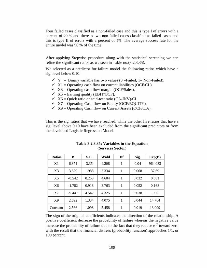
109
Four failed cases classified as a non-failed case and this is type I of errors with a
percent of 20 % and there is two non-failed cases classified as failed cases and
this is type II of errors with a percent of 5%. The average success rate for the
entire model was 90 % of the time.
After applying Stepwise procedure along with the statistical screening we can
refine the significant ratios as we seen in Table no.(3.2.3.35).
We selected as a predictor for failure model the following ratios which have a
sig. level below 0.10:
Y = Binary variable has two values (0 =Failed, 1= Non-Failed).
X1 = Operating cash flow on current liabilities (OCF/CL).
X3 = Operating cash flow margin (OCF/Sales).
X5 = Earning quality (EBIT/OCF).
X6 = Quick ratio or acid-test ratio (CA-INV)/CL.
X7 = Operating Cash flow on Equity (OCF/EQUITY).
X9 = Operating Cash flow on Current Assets (OCF/C.A).
This is the sig. ratios that we have reached, while the other five ratios that have a
sig. level above 0.10 have been excluded from the significant predictors or from
the developed Logistic Regression Model.
Table 3.2.3.35: Variables in the Equation
(Services Sector)
Ratios B S.E. Wald Df Sig. Exp(B)
X1 6.871 3.35 4.208 1 0.04 964.083
X3 3.629 1.988 3.334 1 0.068 37.69
X5 -0.542 0.253 4.604 1 0.032 0.581
X6 -1.782 0.918 3.763 1 0.052 0.168
X7 -9.447 4.542 4.325 1 0.038 .000
X9 2.692 1.334 4.075 1 0.044 14.764
Constant 2.566 1.098 5.458 1 0.019 13.009
The sign of the original coefficients indicates the direction of the relationship. A
positive coefficient decrease the probability of failure whereas the negative value
increase the probability of failure due to the fact that they reduce e-y toward zero
with the result that the financial distress (probability function) approaches 1/1, or
100 percent.
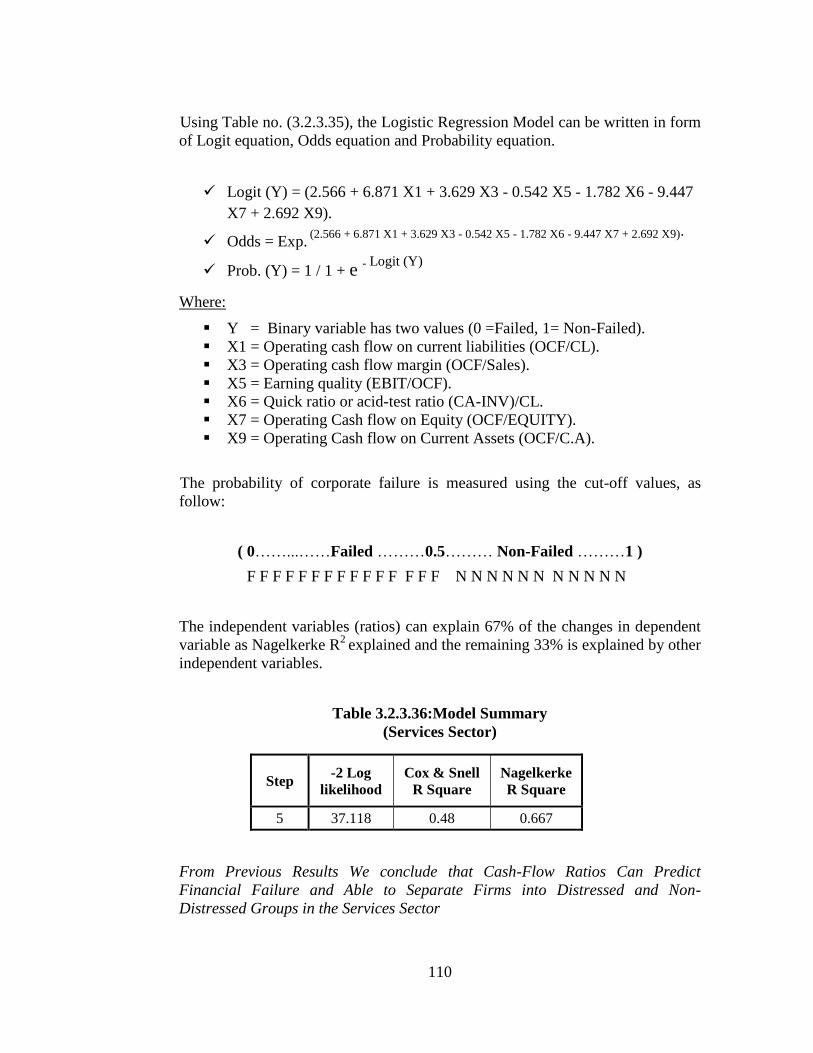
110
Using Table no. (3.2.3.35), the Logistic Regression Model can be written in form
of Logit equation, Odds equation and Probability equation.
Logit (Y) = (2.566 + 6.871 X1 + 3.629 X3 - 0.542 X5 - 1.782 X6 - 9.447
X7 + 2.692 X9).
Odds = Exp. (2.566 + 6.871 X1 + 3.629 X3 - 0.542 X5 - 1.782 X6 - 9.447 X7 + 2.692 X9).
Prob. (Y) = 1 / 1 + e - Logit (Y)
Where:
Y = Binary variable has two values (0 =Failed, 1= Non-Failed).
X1 = Operating cash flow on current liabilities (OCF/CL).
X3 = Operating cash flow margin (OCF/Sales).
X5 = Earning quality (EBIT/OCF).
X6 = Quick ratio or acid-test ratio (CA-INV)/CL.
X7 = Operating Cash flow on Equity (OCF/EQUITY).
X9 = Operating Cash flow on Current Assets (OCF/C.A).
The probability of corporate failure is measured using the cut-off values, as
follow:
( 0……...……Failed ………0.5……… Non-Failed ………1 )
F F F F F F F F F F F F F F F N N N N N N N N N N N
The independent variables (ratios) can explain 67% of the changes in dependent
variable as Nagelkerke R2
explained and the remaining 33% is explained by other
independent variables.
Table 3.2.3.36:Model Summary
(Services Sector)
Step -2 Log
likelihood
Cox & Snell
R Square
Nagelkerke
R Square
5 37.118 0.48 0.667
From Previous Results We conclude that Cash-Flow Ratios Can Predict
Financial Failure and Able to Separate Firms into Distressed and Non-
Distressed Groups in the Services Sector
111
Chapter Four
Study Results , Conclusions and Recommendations
4.1 Study Results
4.2 Study Conclusions
4.3 Study Recommendations
4.4 Study in Future
112
4. Chapter Four: Study Results, Conclusions and
Recommendations
4.1 Study Results
The chapter four shows the study results after theoretical framework and
empirical study on the listed companies have been presented. Also, the study
conclusions and recommendations will be presented.
4.1.1 Results of Testing Hypothesis I
―Hypothesis I tested if there are Differences in Cash-Flow Ratios
between Failed and Non-Failed Companies in PEX‖, we will present the most
important results of hypothesis I for each sector in the study. The univariate
analysis is used to test the first indicators of the predictive variables this is not
mean this measures can predict failure this is the purpose of hypothesis III.
4.1.1.1 Banking Sector
None of the ratios were statistically significant between the two groups,
as the significance for the two-tailed test were above 0.05 for every ratio
except X3, X8 which have a sig. level below 0.05.
X3 = Operating cash flow margin (OCF/Sales),
X8 = Operating Cash flow on Net Income (OCF/N.I).
4.1.1.2 Industrial Sector
The results showed that there are sig. differences in the means of ratios
between failed and non-failed companies in the following ratios,
Operating cash flow divided by current liabilities (X1), Cash flow
coverage of interest (X2), Operating cash flow margin (X3), Operating
cash flow return on total assets (X4), Operating cash flow return on
Equity (X7), Operating cash flow return on Net Income (X8), Operating
cash flow return on Free cash flow (X10) and Operating cash flow return
on current Assets (X11).
4.1.1.3 Insurance Sector
The results showed that there are sig. differences in the means of ratios
between failed and non-failed companies in the following ratios,
Operating cash flow divided by current liabilities (X1), Operating cash
flow margin (X3), Operating cash flow return on total assets (X4), Quick
ratio (X6) and Operating cash flow return on current Assets (X11).
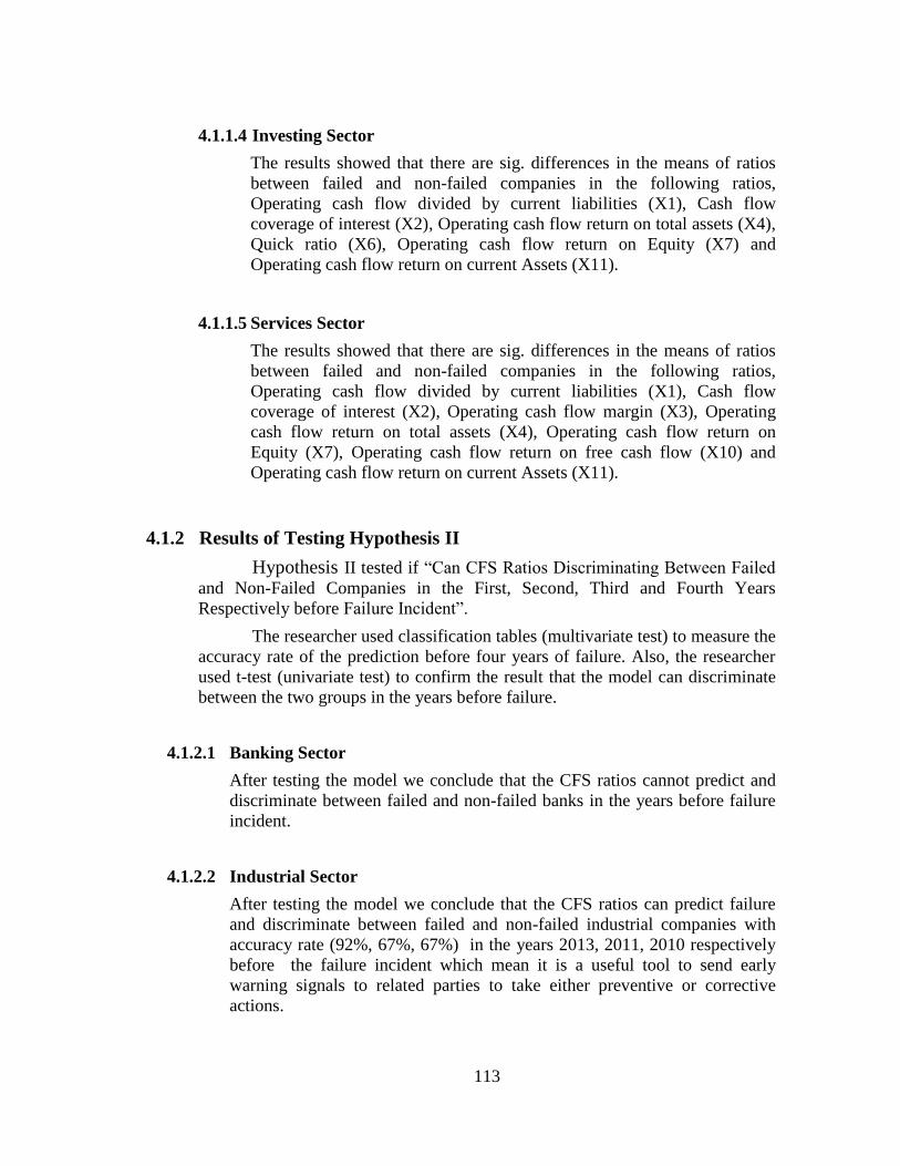
113
4.1.1.4 Investing Sector
The results showed that there are sig. differences in the means of ratios
between failed and non-failed companies in the following ratios,
Operating cash flow divided by current liabilities (X1), Cash flow
coverage of interest (X2), Operating cash flow return on total assets (X4),
Quick ratio (X6), Operating cash flow return on Equity (X7) and
Operating cash flow return on current Assets (X11).
4.1.1.5 Services Sector
The results showed that there are sig. differences in the means of ratios
between failed and non-failed companies in the following ratios,
Operating cash flow divided by current liabilities (X1), Cash flow
coverage of interest (X2), Operating cash flow margin (X3), Operating
cash flow return on total assets (X4), Operating cash flow return on
Equity (X7), Operating cash flow return on free cash flow (X10) and
Operating cash flow return on current Assets (X11).
4.1.2 Results of Testing Hypothesis II
Hypothesis II tested if ―Can CFS Ratios Discriminating Between Failed
and Non-Failed Companies in the First, Second, Third and Fourth Years
Respectively before Failure Incident‖.
The researcher used classification tables (multivariate test) to measure the
accuracy rate of the prediction before four years of failure. Also, the researcher
used t-test (univariate test) to confirm the result that the model can discriminate
between the two groups in the years before failure.
4.1.2.1 Banking Sector
After testing the model we conclude that the CFS ratios cannot predict and
discriminate between failed and non-failed banks in the years before failure
incident.
4.1.2.2 Industrial Sector
After testing the model we conclude that the CFS ratios can predict failure
and discriminate between failed and non-failed industrial companies with
accuracy rate (92%, 67%, 67%) in the years 2013, 2011, 2010 respectively
before the failure incident which mean it is a useful tool to send early
warning signals to related parties to take either preventive or corrective
actions.
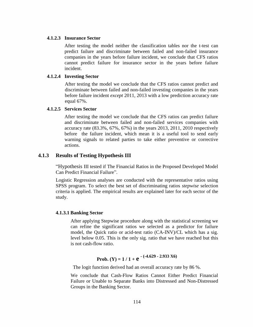
114
4.1.2.3 Insurance Sector
After testing the model neither the classification tables nor the t-test can
predict failure and discriminate between failed and non-failed insurance
companies in the years before failure incident, we conclude that CFS ratios
cannot predict failure for insurance sector in the years before failure
incident.
4.1.2.4 Investing Sector
After testing the model we conclude that the CFS ratios cannot predict and
discriminate between failed and non-failed investing companies in the years
before failure incident except 2011, 2013 with a low prediction accuracy rate
equal 67%.
4.1.2.5 Services Sector
After testing the model we conclude that the CFS ratios can predict failure
and discriminate between failed and non-failed services companies with
accuracy rate (83.3%, 67%, 67%) in the years 2013, 2011, 2010 respectively
before the failure incident, which mean it is a useful tool to send early
warning signals to related parties to take either preventive or corrective
actions.
4.1.3 Results of Testing Hypothesis III
―Hypothesis III tested if The Financial Ratios in the Proposed Developed Model
Can Predict Financial Failure‖.
Logistic Regression analyses are conducted with the representative ratios using
SPSS program. To select the best set of discriminating ratios stepwise selection
criteria is applied. The empirical results are explained later for each sector of the
study.
4.1.3.1 Banking Sector
After applying Stepwise procedure along with the statistical screening we
can refine the significant ratios we selected as a predictor for failure
model, the Quick ratio or acid-test ratio (CA-INV)/CL which has a sig.
level below 0.05. This is the only sig. ratio that we have reached but this
is not cash-flow ratio.
Prob. (Y) = 1 / 1 + e - (-4.629 - 2.933 X6)
The logit function derived had an overall accuracy rate by 86 %.
We conclude that Cash-Flow Ratios Cannot Either Predict Financial
Failure or Unable to Separate Banks into Distressed and Non-Distressed
Groups in the Banking Sector.
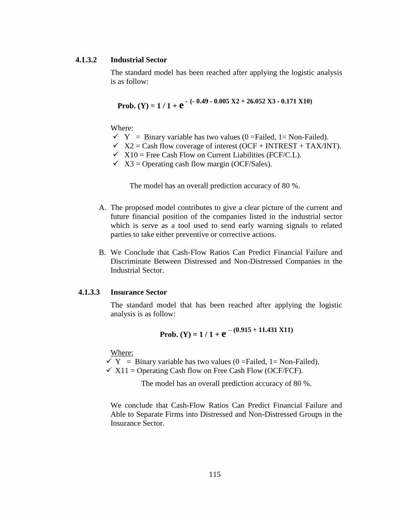
115
4.1.3.2 Industrial Sector
The standard model has been reached after applying the logistic analysis
is as follow:
Prob. (Y) = 1 / 1 + e - (- 0.49 - 0.005 X2 + 26.052 X3 - 0.171 X10)
Where:
Y = Binary variable has two values (0 =Failed, 1= Non-Failed).
X2 = Cash flow coverage of interest (OCF + INTREST + TAX/INT).
X10 = Free Cash Flow on Current Liabilities (FCF/C.L).
X3 = Operating cash flow margin (OCF/Sales).
The model has an overall prediction accuracy of 80 %.
A. The proposed model contributes to give a clear picture of the current and
future financial position of the companies listed in the industrial sector
which is serve as a tool used to send early warning signals to related
parties to take either preventive or corrective actions.
B. We Conclude that Cash-Flow Ratios Can Predict Financial Failure and
Discriminate Between Distressed and Non-Distressed Companies in the
Industrial Sector.
4.1.3.3 Insurance Sector
The standard model that has been reached after applying the logistic
analysis is as follow:
Prob. (Y) = 1 / 1 + e – (0.915 + 11.431 X11)
Where:
Y = Binary variable has two values (0 =Failed, 1= Non-Failed).
X11 = Operating Cash flow on Free Cash Flow (OCF/FCF).
The model has an overall prediction accuracy of 80 %.
We conclude that Cash-Flow Ratios Can Predict Financial Failure and
Able to Separate Firms into Distressed and Non-Distressed Groups in the
Insurance Sector.
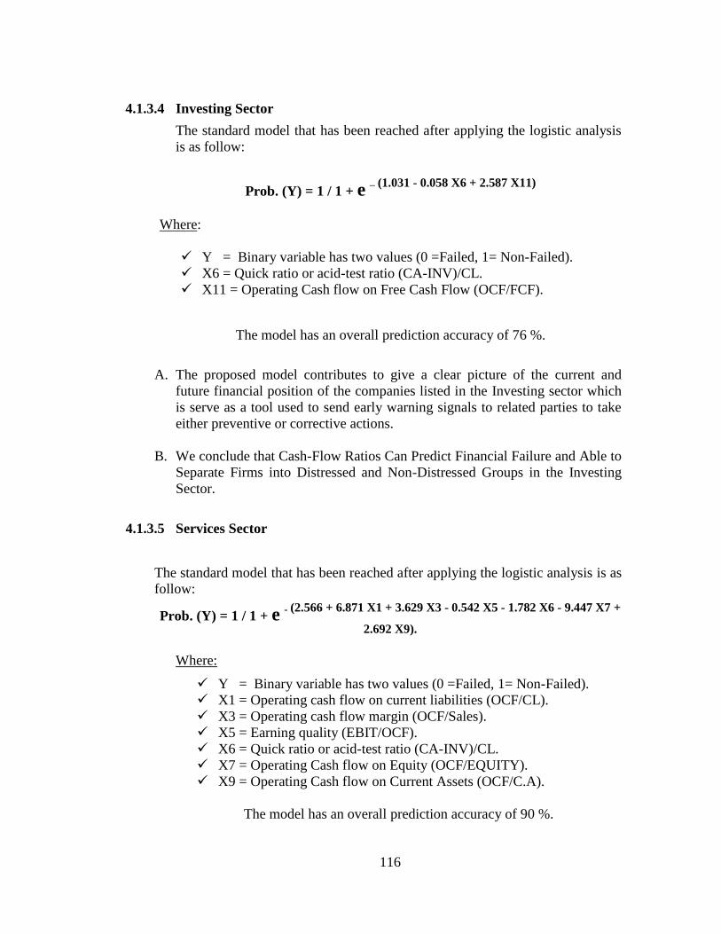
116
4.1.3.4 Investing Sector
The standard model that has been reached after applying the logistic analysis
is as follow:
Prob. (Y) = 1 / 1 + e – (1.031 - 0.058 X6 + 2.587 X11)
Where:
Y = Binary variable has two values (0 =Failed, 1= Non-Failed).
X6 = Quick ratio or acid-test ratio (CA-INV)/CL.
X11 = Operating Cash flow on Free Cash Flow (OCF/FCF).
The model has an overall prediction accuracy of 76 %.
A. The proposed model contributes to give a clear picture of the current and
future financial position of the companies listed in the Investing sector which
is serve as a tool used to send early warning signals to related parties to take
either preventive or corrective actions.
B. We conclude that Cash-Flow Ratios Can Predict Financial Failure and Able to
Separate Firms into Distressed and Non-Distressed Groups in the Investing
Sector.
4.1.3.5 Services Sector
The standard model that has been reached after applying the logistic analysis is as
follow:
Prob. (Y) = 1 / 1 + e - (2.566 + 6.871 X1 + 3.629 X3 - 0.542 X5 - 1.782 X6 - 9.447 X7 +
2.692 X9).
Where:
Y = Binary variable has two values (0 =Failed, 1= Non-Failed).
X1 = Operating cash flow on current liabilities (OCF/CL).
X3 = Operating cash flow margin (OCF/Sales).
X5 = Earning quality (EBIT/OCF).
X6 = Quick ratio or acid-test ratio (CA-INV)/CL.
X7 = Operating Cash flow on Equity (OCF/EQUITY).
X9 = Operating Cash flow on Current Assets (OCF/C.A).
The model has an overall prediction accuracy of 90 %.
117
A. The proposed model contributes to give a clear picture of the current and
future financial position of the companies listed in the services sector which is
serve as a tool used to send early warning signals to related parties to take
either preventive or corrective actions.
B. We conclude that Cash-Flow Ratios Can Predict Financial Failure and Able to
Separate Firms into Distressed and Non-Distressed Groups in the Services
Sector.
4.1.4 Other Results
A. After reviewing past studies the researcher concluded the best model for
predicting corporate failure is by using cash flow-based measures and
logistical analysis method which increase the predictive ability of the model
before financial failure incident. This study agreed with the previous studies
for (Quarcoo & Smedberg, 2014), (Bhandari & Iyer, 2013), (Alawi &
Gharaibeh, 2008), (Charitou, Neophytou, & Charalambous, 2004), (Matar &
Obaidat, 2007), (Rodgers, 2013) which concluded that the cash flow-based
models outperformed the accrual-based models and did not agree with these
studies (Quarcoo & Smedberg, 2014), ( Mazouz, Crane, & Gambre, 2012),
(Shkurti & Duraj, 2010) which concluded that the cash flow models did not
improve business failure prediction.
B. Discriminant analysis (DA) was most widely used technique by (AbuMoamer,
2014), (Enshassi, Al-Hallaq, & Mohamed, 2006), ( Mazouz, Crane, &
Gambre, 2012), (Shkurti & Duraj, 2010), (Amendola, Bisogno, Restaino, &
Sensini, 2011), (Rugby, 2006). Also, Altman and Kida‘s models were used by
(Alkhatib & Al Bzour, 2011) and (Rammo & Al-Wattar, 2010) that required
restricted assumptions that cannot be applied to this study.
C. Logistical models were used by (Ghusain, 2004), (Charitou, Neophytou, &
Charalambous, 2004) and (Rugby, 2006). The sample that has been used in
these studies was unbalanced sample of companies with less restrictive
assumptions were required in these models. These advantages encouraged the
researcher to use the logistic model.
118
4.2 Study Conclusions
A. The cash-flow based ratios have significant predictive power to predict
corporate failure.
B. Despite the great benefit generated by the mathematical models based on
the financial ratios and regardless of the ability of these models to predict
financial failure, there are many reasons that leading companies to failure.
Therefore, it does not require only mathematical models as a single tool
to assess the ability of the public shareholding companies to continue, but
these models must be linked with any additional information (non-
financial indicators) beside factors related to external and internal
environment for these companies.
C. The study confirms what have been reached by other researchers on not
restricting the prediction of the financial failure on the traditional
financial ratios (accrual-based) derived from balance sheet and income
statement but failure models must include ratios selected from a cash flow
statement (cash flow-based).
D. The models that have been developed for each economic sector have
common financial ratios that have been used to discriminate companies
and to predict failure as in both insurance and investment sectors for the
financial ratio, X11= Operating Cash flow on Free Cash Flow
(OCF/FCF) which seem it has a significant discrimination power for
companies. Also, the financial ratio X3 = Operating cash flow margin
(OCF/Sales) has significant discrimination power for companies in both
industrial and services sectors.
E. The high prediction accuracy rates for the models that have been reached,
which means the high ability of these models to predict the failure.
F. The models that have been reached will help in sending early warning
signals that concern interested parties such as investors, creditors,
suppliers, management, government agencies offering them the advantage
to take either preventive or corrective actions.
119
4.3 Study Recommendations
From the results of this study, the study recommends the following:
A. The companies that applied to be listed in the PEX should to adhering
International Financial Reporting Standards, issuing audited financial
statements and to follow the same accounting procedures as it is stated in
the PEX listing regulation in articles no. (7) and no. (8), so the models
that have been reached can be applied without problems.
B. The financial intermediation offices in the PEX have to consider
utilization of the models that have been reached by the researcher for
each sector in the PEX as it facilitates the assessment of companies‘
performance in addition to predicting the possibility of failure and to send
early warning signals to take corrective or preventive actions.
C. The investors have to consider utilization of the models that have been
reached for each sector to help them in avoiding risky investments and
reduce the risk of losing their money in the PEX.
D. The government agencies have to consider utilization of the models that
have been reached for detecting companies that may bankrupt in the
future in order to help them in avoiding financial crises in the PEX and
maintain economic stability.
E. The auditors have to consider utilization of the models that have been
reached in assessing company‘s ability to continue as a ―going concern‖.
F. Creditors and suppliers have to consider utilization of the models that
have been reached to assess the liquidity position of the debtor firm.
G. To conduct more studies in predicting business failure using cash-flow
based measures and to give more concern in cash flow statement
measures.
120
4.4 Research in Future
Based on the findings and results of this study there are some suggestions
for future researches.
The prediction of business failure has been largely investigated in the
literature over the last few decades from both theoretical and empirical side.
It is recommended further studies in this area where this study considered
from the eminent studies in the field of companies failure prediction by using
cash-flow based measures and the statistical method the logistic model.
The researcher recommends the following future researches for PhD and MBA
students:
A. Predicting Corporate Bankruptcy Using Multiple Discriminant Analysis
on the Listed Companies in the PEX.
B. Predicting Corporate Bankruptcy Using Neural Network Models on the
Listed Companies in the PEX.
C. Predicting Corporate Bankruptcy Using Altman and Kida Models on the
Listed Companies in the PEX.
D. Prediction of Business Failure: a Comparison of Discriminant and
Logistic Regression Analyses.
E. Predicting Corporate Bankruptcy on Private Companies.
121
5. Bibliography
First: Arabic References
Books
1. Miqdad, M., & al-Farra, M. (2012). Scientific Research Methodology and
Statistical Analysis in Managerial and Economic Sciences. Gaza, Palestine:
Dar Al-Miqdad for Printing.
2. Miqdad, M. I. (2014). Economic Measurement and Data Analysis (2 Ed.).
Gaza, Palestine: Dar Al-Miqdad for Printing.
Periodicals
1. Alawi, S., & Gharaibeh, F. (2008). Predicting Corporate Distress in Jordan:
A Multidimensional Scaling Approach. Journal of Management Science
Studies, 35(2), 337-397.
2. Alkhatib, K., & Al Bzour, A. E. (2011). Predicting Corporate Bankruptcy of
Jordanian Listed Companies: Using Altman and Kida Models. International
Journal of Business and Management, 6(3), pp. 208-215.
3. Ashour, Y. H., & El-Farra, M. M. (2002). Business Failure in the Gaza Strip
Bankers and Business Experts' Viewpoints. Journal of the Islamic University
of Gaza, 10(1), pp. 2-24.
4. Enshassi, A., Al-Hallaq, K., & Mohamed, S. (2006). Causes of Contractor's
Business Failure in Developing Countries: The Case of Palestine. Journal of
Construction in Developing Countries, 11(2).
5. Matar, M., & Obaidat, A. (2007). The Role of Cash Flow Ratios in
Improving the Accuracy of Models Based on Accrual Ratios to Predict the
Financial Failure of Jordanian Industrial Companies Shareholders. Jordanian
Journal in Business Administration, 3(4), pp. 440-462.
6. Rammo, W. M., & Al-Wattar, S. A. (2010). Using Financial Analysis
Techniques to Predict the Failure of Contributing Industrial Companies: A
study of a Sample Consisting of Iraqi Contributing Industrial Companies
Listed in Iraqi Stock Market. Rafdeen Tanmia Journal, 32(100), pp. 9-29.
7. Rugby, M. T. (2006). The Use of Financial Ratios to Predict Failure of
Jordanian Public Shareholding Companies Using Discriminant and Logit
Analysis. Arab Journal of Managerial Sciences, 13(2), pp. 149-173.
8. Zaki, E., Bah, R., & Rao, A. (2011). Assessing Probabilities of Financial
Distress of Banks in UAE. International Journal of Managerial Finance,
7(3), pp. 304-320.
122
Thesis
1. Ataiwiel, A. (2008). The Extent to Which the Banks Depend on the Financial
Analysis to Predict Failure: An Empirical Study on the National Commercial
Banks in the Gaza Strip. (Master Thesis). Gaza, Palestine: Islamic Unversity
of Gaza.
2. Ghusain, H. (2004). The Use of Financial Ratios to Predict Corporate Failure:
Empirical Study on the Construction Sector in the Gaza Strip. (Master thesis).
Gaza, Palestine: The Islamic University of Gaza.
Conference Proceedings
1. El Khoury, R., & Al Beaïno, R. (2014). Classifying Manufacturing Firms in
Lebanon: An Application of Altman‘s Model. 2nd World Conference on
Business, Economics And Management, (pp. 11-18). Lebanon.
2. AbuMoamer, F. M. (2014). Corporate Bankruptcy Prediction and Equity
Returns in Palestinian Banks. 11th EBES Conference. Istanbul-Turkey:
https://www.researchgate.net.
Second: Foreign References
Books
1. Altman, E. (1993). In Corporate Financial Distress and Bankruptcy (2 Ed.).
New York, NY: John Wiley & Sons, Inc.
2. Altman, E. I., & Hotchkiss, E. (2006). Predict and Avoid Bankruptcy, Analyse
and Invest in Distressed Debt (3 Ed.). Hoboken, New Jersey, USA: John
Wiley & Sons.
3. Bragg, S. M. (2002). Business Ratios and Formulas: A Comprehensive
Guide. USA: John Wiley & Sons.
4. Brigham, E. F., & Houston, J. F. (2004). Fundamentals of Financial
Management (4 Ed.). Ohio City: South-Western, Mason, OH.
5. Ehrhardt, M. C., & Brigham, E. F. (2011). Financial Management: Theory
and Practice (13 Ed.). USA: South-Western Cengage Learning.
6. Gitman, L. (2002). Principles of Managerial Finance (10 Ed.). New Jersey,
USA: Addison Wesley.
7. McLaney, E. (2009). Business Finance: Theory and Practice (8 Ed.).
England: Pearson Education Ltd.
8. Paramasivan, C., & Subramanian, T. (2008). Financial Management. USA:
New Age International Pvt Ltd.
123
Periodicals
1. Altman, E. (1968). Financial ratios, discriminate analysis and the prediction of
corporate bankruptcy. Journal of Finance, 23(4), pp. 589–609.
2. Altman, E. I. (1970). Ratio Analysis and the Prediction of Firm Failure: A
Reply. The Journal of Finance, 25(5), pp. 1169-1172.
3. Altman, E. I. (1984). The Success of Business Failure Prediction Models: An
International Survey. Journal of Banking and Finance, 8(2), pp. 171-198.
4. Amendola, A., Bisogno, M., Restaino, M., & Sensini, L. (2011). Forecasting
Corporate Bankruptcy: Empirical Evidence on Italian Data. EuroMed Journal
of Business, 6(3), pp. 294-312.
5. Beaver, W. H. (1966). Financial Ratios as Predictors of Failure. Journal of
Accounting, 4(3), pp. 71-111.
6. Beaver, W. H. (1968). Alternative Accounting Measures as Predictors of
Failure. Journal of Accounting Review, 43(1), pp. 113-122.
7. Bhandari, S., & Iyer, R. (2013). Predicting Business Failure Using Cash Flow
Statement Based Measures. Managerial Finance Journal, 39(7), pp. 667-676.
8. Charitou, A., Neophytou, E., & Charalambous, C. (2004). Predicting
Corporate Failure: Empirical Evidence for the UK. European Accounting
Review Journal, 13(3), pp. 465-497.
9. Chitnomrath, T., Evans, R., & Christopher, T. (2011). Corporate governance
and post-bankruptcy reorganisation performance Evidence from Thailand.
Asian Review of Accounting, 19(1), pp. 50-67.
10. Dikmen, I. l., Birgonul, M. T., Ozorhon, B., & Sapci, N. E. (2010). Using
Analytic Network Process to Assess Business Failure Risks of Construction
Firms. Engineering, Construction and Architectural Management, 17(4), pp.
369-386.
11. Hines, C., Kreuze, J., & Langsam, S. (2011). An analysis of Lehman Brothers
bankruptcy and Repo 105 transactions. American Journal of Business, 26(1),
pp. 40-49.
12. Mazouz, A., Crane, K., & Gambre, P. (2012). The Impact of Cash Flow on
Business Failure Analysis and Prediction. International Journal of Business,
Accounting, and Finance, 6(2), pp. 68-81.
13. Purnanandam, A. . (2008). Financial distress and corporate risk management:
theory and evidence. Journal of Financial Economics, 87, pp. 706-39.
14. Senbet, L. W., & Wang, T. Y. (2010). Corporate Financial Distress and
Bankruptcy: A Survey. Foundations and Trends in Finance, 5(4), pp. 243-335.
15. Shkurti, R., & Duraj, B. (2010). Using Multiple Discriminant Analysis in The
Bankruptcy Prediction in Albania- A Study With The State-Owned
Enterprises. Journal of Academic Research in Economics, 2(1), pp. 36-64.
16. Vuran, B. (2009). Prediction of Business Failure: A Comparison of
Discriminant and Logistic Regression Analyses. Istanbul University Journal
of the School of Business Administration, 38(1), pp. 47-65.
124
Thesis
1. Danilov, K. (2014). Corporate Bankruptcy: Assessment, Analysis and
Prediction of Financial Distress, Insolvency, and Failure. (Master Thesis).
USA: MIT Sloan School of Management.
2. Kpodoh, B. (2010). Bankruptcy and Financial Distress Prediction in the
Mobile Telecom Industry. (Master Thesis). Sweden, Retrieved from
3. http://www.bth.se/fou/cuppsats.nsf/6753b78eb2944e0ac1256608004f0535/62
20c84cf827480ec12577340049504b?OpenDocument: Blekinge Institute of
Technology.
4. Onyiri, S. (2014). Predicting Financial Distress using Altman‘s Z-score and
the Sustainable Growth Rate. (PhD). Arizona, USA: Northcentral University.
5. Quarcoo, N. L., & Smedberg, P. (2014). The Road to Bankruptcy: A Study on
Predicting Financial Distress in Sweden. (Master Thesis). Sweden: Umeå
School of Business and Economics.
6. Rodgers, C. S. (2013). Predicting Corporate Bankruptcy Using Multivariant
Discriminant Analysis, Logistic Regression and Operating Cash Flow Ratio
Analysis. (PhD). San Francisco, CA: Golden Gate University.
Third: Web Sites
1. Ames, M. (2013). Small Business Management. Retrieved January 25, 2015,
from https://www.sba.gov/content/what-are-major-reasons-small-business-
failure
2. About Money. (2015). Retrieved October 10, 2015, from About Money:
http://bizfinance.about.com/od/cashflowanalysis/tp/cash-flow-ratios.htm
3. BankruptcyData.com. (2015). Retrieved March 16, 2015, from
http://www.bankruptcydata.com/largest.asp?y=
4. Instantshift. (2010). Retrieved March 16, 2015, from 22 Largest Bankruptcies
in World History: http://www.instantshift.com/2010/02/03/22-largest-
bankruptcies-in-world-history
5. Investopedia. (2015). Retrieved March 06, 2015, from Investopedia:
http://www.investopedia.com/terms/b/bankruptcy.asp
6. Palestine Exchange. (2015). Retrieved March 30, 2015, from
http://www.pex.ps
7. Wikipedia. (2015). Retrieved March 06, 2015, from
http://encyclopedia.thefreedictionary.com/Financial+distress
8. Palestine Exchange. (2015). Retrieved July 22, 2015, from
http://www.pex.ps/PSEWebSite/publications/PEX-Listing-Regulation-
English.pdf
125
Appendix (1)
6.1 Observed Groups and Predicted Probabilities
6.1.1 Banking Sector
6.1.2 Industry Sector
6.1.3 Insurance Sector
6.1.4 Investing Sector
6.1.5 Services Sector
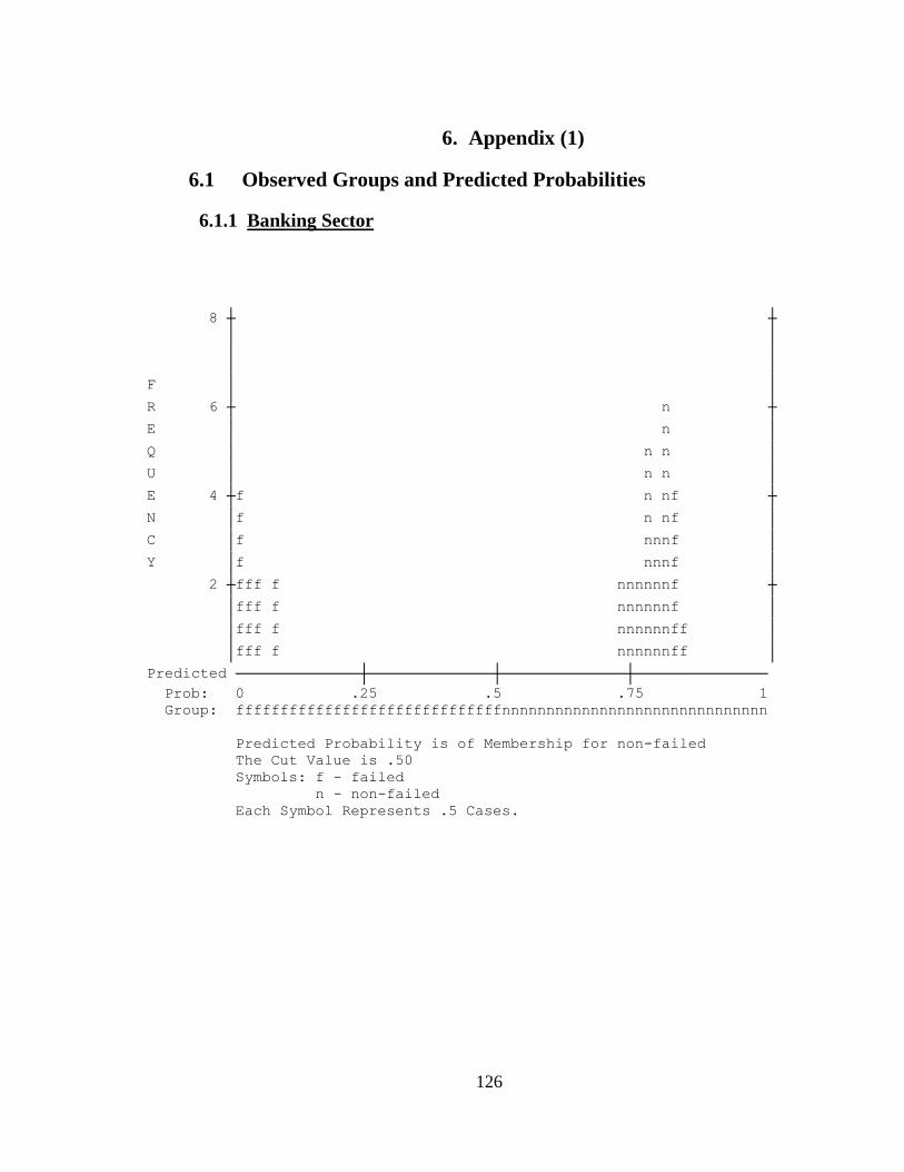
126
6. Appendix (1)
6.1 Observed Groups and Predicted Probabilities
6.1.1 Banking Sector
8
F
R 6 n
E n
Q n n
U n n
E 4 f n nf
N f n nf
C f nnnf
Y f nnnf
2 fff f nnnnnnf
fff f nnnnnnf
fff f nnnnnnff
fff f nnnnnnff
Predicted
Prob: 0 .25 .5 .75 1
Group: ffffffffffffffffffffffffffffffnnnnnnnnnnnnnnnnnnnnnnnnnnnnnn
Predicted Probability is of Membership for non-failed
The Cut Value is .50
Symbols: f - failed
n - non-failed
Each Symbol Represents .5 Cases.
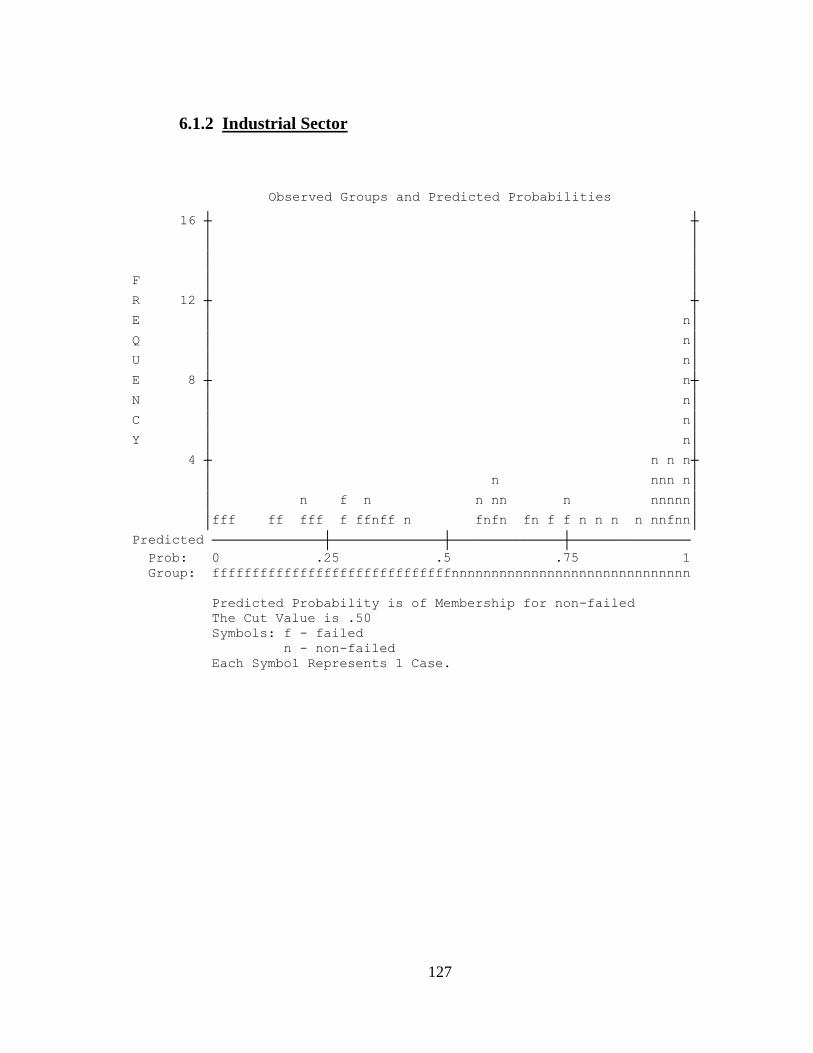
127
6.1.2 Industrial Sector
Observed Groups and Predicted Probabilities
16
F
R 12
E n
Q n
U n
E 8 n
N n
C n
Y n
4 n n n
n nnn n
n f n n nn n nnnnn
fff ff fff f ffnff n fnfn fn f f n n n n nnfnn
Predicted
Prob: 0 .25 .5 .75 1
Group: ffffffffffffffffffffffffffffffnnnnnnnnnnnnnnnnnnnnnnnnnnnnnn
Predicted Probability is of Membership for non-failed
The Cut Value is .50
Symbols: f - failed
n - non-failed
Each Symbol Represents 1 Case.
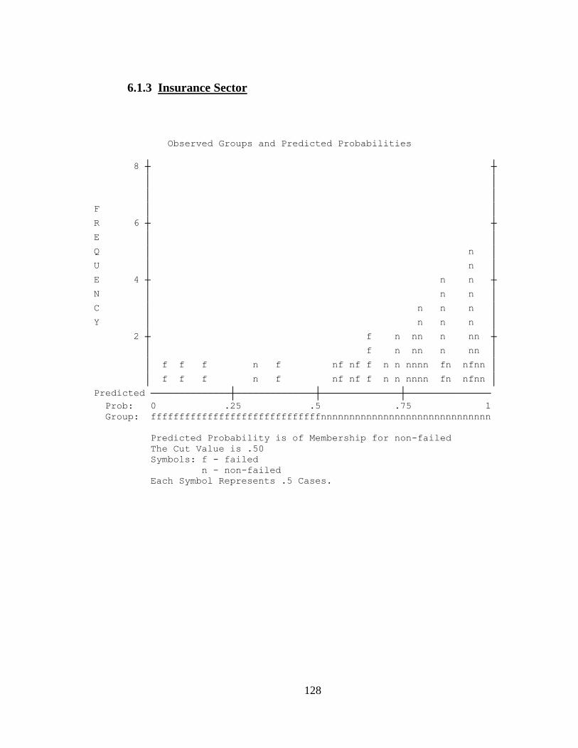
128
6.1.3 Insurance Sector
Observed Groups and Predicted Probabilities
8
F
R 6
E
Q n
U n
E 4 n n
N n n
C n n n
Y n n n
2 f n nn n nn
f n nn n nn
f f f n f nf nf f n n nnnn fn nfnn
f f f n f nf nf f n n nnnn fn nfnn
Predicted
Prob: 0 .25 .5 .75 1
Group: ffffffffffffffffffffffffffffffnnnnnnnnnnnnnnnnnnnnnnnnnnnnnn
Predicted Probability is of Membership for non-failed
The Cut Value is .50
Symbols: f - failed
n - non-failed
Each Symbol Represents .5 Cases.
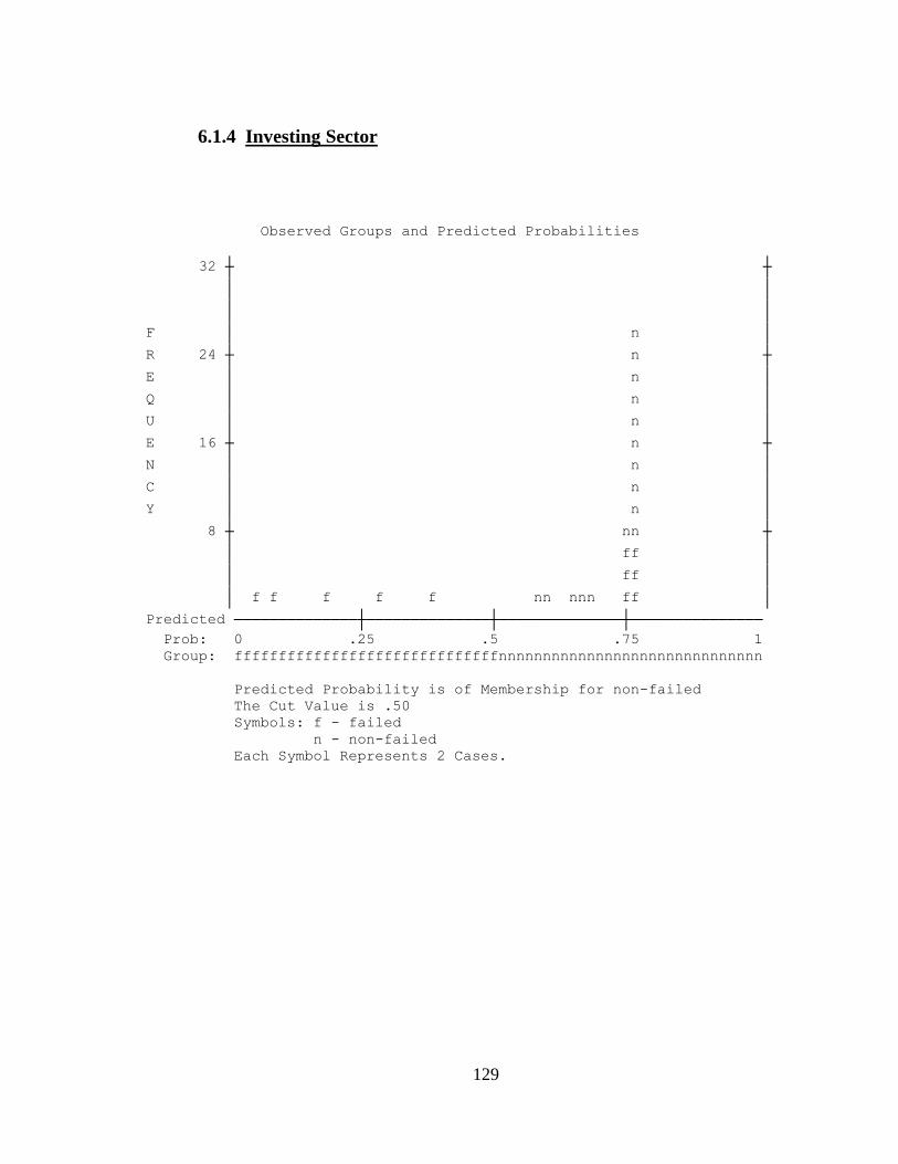
129
6.1.4 Investing Sector
Observed Groups and Predicted Probabilities
32
F n
R 24 n
E n
Q n
U n
E 16 n
N n
C n
Y n
8 nn
ff
ff
f f f f f nn nnn ff
Predicted
Prob: 0 .25 .5 .75 1
Group: ffffffffffffffffffffffffffffffnnnnnnnnnnnnnnnnnnnnnnnnnnnnnn
Predicted Probability is of Membership for non-failed
The Cut Value is .50
Symbols: f - failed
n - non-failed
Each Symbol Represents 2 Cases.
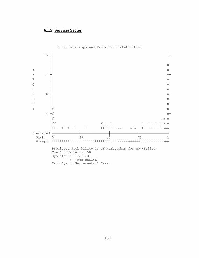
130
6.1.5 Services Sector
Observed Groups and Predicted Probabilities
16
n
F n
R 12 n
E n
Q n
U n
E 8 n
N n
C n
Y f n
4 f n
f nn n
ff fn n n nnn n nnn n
ff n f f f f ffff f n nn nfn f nnnnn fnnnn
Predicted
Prob: 0 .25 .5 .75 1
Group: ffffffffffffffffffffffffffffffnnnnnnnnnnnnnnnnnnnnnnnnnnnnnn
Predicted Probability is of Membership for non-failed
The Cut Value is .50
Symbols: f - failed
n - non-failed
Each Symbol Represents 1 Case.
131
Appendix (2)
7.1 Financial Ratios
7.1.1 Banking Sector
7.1.2 Industrial Sector
7.1.3 Insurance Sector
7.1.4 Investing Sector
7.1.5 Services Sector
7.2 Economic Sectors
7.2.1 Economic Sectors
7.2.2 Banking Sector
7.2.3 Industrial Sector
7.2.4 Insurance Sector
7.2.5 Investing Sector
7.2.6 Services Sector
7.3 Group Membership
7.3.1 Banking Sector
7.3.2 Industrial Sector
7.3.3 Insurance Sector
7.3.4 Investing Sector
7.3.5 Services Sector
7.4 Multicollinearity Test
7.4.1 Banking Sector
7.4.2 Industrial Sector
7.4.3 Insurance Sector
7.4.4 Investing Sector
7.4.5 Services Sector
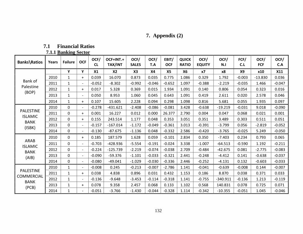
132
7. Appendix (2)
7.1 Financial Ratios 7.1.1 Banking Sector
Banks\Ratios Years Failure OCF OCF/
CL OCF+INT.+ TAX/INT
OCF/ SALES
OCF/ T.A
EBIT/ OCF
QUICK RATIO
OCF/ EQUITY
OCF/ N.I
FCF/ C.L
OCF/ FCF
OCF/ C.A
Bank of Palestine
(BOP)
Y Y X1 X2 X3 X4 X5 X6 x7 x8 X9 x10 X11
2010 1 + 0.039 16.070 0.873 0.035 0.775 1.086 0.329 1.792 -0.003 -13.830 0.036
2011 1 - -0.052 -8.302 -0.992 -0.046 -0.652 1.097 -0.388 -2.219 -0.035 1.466 -0.047
2012 1 + 0.017 5.328 0.369 0.015 1.934 1.091 0.140 0.806 0.054 0.323 0.016
2013 1 - 0.050 8.953 1.060 0.045 0.643 1.091 0.419 2.611 0.020 2.578 0.046
2014 1 + 0.107 15.605 2.228 0.094 0.298 1.098 0.816 5.681 0.055 1.935 0.097
PALESTINE ISLAMIC
BANK (ISBK)
2010 0 - -0.278 -431.621 -2.408 -0.086 -0.081 3.428 -0.638 -19.219 -0.031 9.018 -0.090
2011 0 + 0.001 16.227 0.012 0.000 26.377 2.790 0.004 0.047 0.068 0.021 0.001
2012 0 + 0.155 243.514 1.177 0.048 0.353 3.051 0.351 3.489 0.303 0.511 0.051
2013 0 - -0.157 -167.014 -1.172 -0.049 -0.361 3.013 -0.391 -3.799 0.056 -2.819 -0.052
2014 0 - -0.130 -87.675 -1.136 0.048 -0.332 2.586 -0.420 -3.765 -0.025 5.249 -0.050
ARAB ISLAMIC
BANK (AIB)
2010 0 + 0.185 187.579 1.628 0.059 -0.101 2.834 0.350 -7.403 0.234 0.793 0.065
2011 0 - -0.703 -428.936 -5.554 -0.191 -0.024 3.338 -1.007 -64.513 -0.590 1.192 -0.211
2012 0 - -0.224 -125.739 -2.219 -0.074 -0.038 2.709 -0.484 -42.675 0.081 -2.775 -0.083
2013 0 - -0.090 -59.376 -1.101 -0.033 -0.321 2.441 -0.248 -4.412 0.141 -0.638 -0.037
2014 0 - -0.080 -49.041 -1.029 -0.030 -0.336 2.446 -0.252 -4.131 0.132 -0.603 -0.033
PALESTINE COMMERCIAL
BANK (PCB)
2010 1 - -0.008 0.245 -0.213 -0.007 -2.786 1.141 -0.041 -0.639 -0.008 0.144 -0.007
2011 1 + 0.038 4.838 0.896 0.031 0.432 1.153 0.186 8.870 0.038 0.371 0.033
2012 1 - -0.136 -9.648 -3.453 -0.114 -0.318 1.141 -0.755 -340.911 -0.136 1.213 -0.119
2013 1 + 0.078 9.358 2.457 0.068 0.133 1.102 0.568 140.831 0.078 0.725 0.071
2014 1 - -0.051 -3.766 -1.430 -0.044 -0.328 1.114 -0.342 -10.355 -0.051 1.045 -0.046
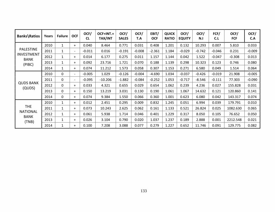
133
Banks\Ratios Years Failure OCF OCF/
CL OCF+INT.+ TAX/INT
OCF/ SALES
OCF/ T.A
EBIT/ OCF
QUICK RATIO
OCF/ EQUITY
OCF/ N.I
FCF/ C.L
OCF/ FCF
OCF/ C.A
PALESTINE INVESTMENT
BANK (PIBC)
2010 1 + 0.040 8.464 0.771 0.031 0.408 1.201 0.132 10.293 0.007 5.810 0.033
2011 1 - -0.011 0.016 -0.191 -0.008 -2.361 1.184 -0.029 -0.742 -0.046 0.231 -0.009
2012 1 + 0.014 6.177 0.275 0.011 1.157 1.144 0.042 1.522 -0.047 -0.308 0.013
2013 1 + 0.092 23.716 1.721 0.070 0.188 1.139 0.298 10.323 0.123 0.746 0.080
2014 1 + 0.074 11.212 1.573 0.058 0.307 1.153 0.271 6.580 0.049 1.514 0.064
QUDS BANK (QUDS)
2010 0 - -0.005 1.029 -0.126 -0.004 -4.690 1.034 -0.037 -0.426 -0.019 21.908 -0.005
2011 0 - -0.095 -10.206 -1.882 -0.084 -0.252 1.053 -0.717 -8.546 -0.111 77.303 -0.090
2012 0 + 0.033 4.321 0.655 0.029 0.654 1.062 0.239 4.236 0.027 155.828 0.031
2013 0 + 0.150 13.219 3.031 0.130 0.190 1.061 1.067 14.632 0.121 120.860 0.141
2014 0 + 0.074 9.384 1.550 0.066 0.360 1.001 0.623 6.080 0.042 143.317 0.074
THE NATIONAL
BANK (TNB)
2010 1 + 0.012 2.451 0.295 0.009 0.832 1.245 0.051 6.994 0.039 179.791 0.010
2011 1 + 0.073 10.243 2.625 0.062 0.161 1.133 0.521 26.824 0.025 1082.630 0.065
2012 1 + 0.061 5.938 1.714 0.046 0.401 1.229 0.317 8.050 0.105 76.652 0.050
2013 1 + 0.026 3.104 0.790 0.020 1.037 1.237 0.189 2.888 0.001 2212.548 0.021
2014 1 + 0.100 7.208 3.088 0.077 0.279 1.227 0.652 11.746 0.091 129.775 0.082
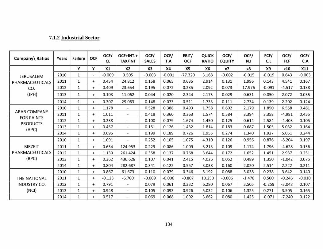
134
7.1.2 Industrial Sector
Company\ Ratios Years Failure OCF OCF/
CL OCF+INT.+ TAX/INT
OCF/ SALES
OCF/ T.A
EBIT/ OCF
QUICK RATIO
OCF/ EQUITY
OCF/ N.I
FCF/ C.L
OCF/ FCF
OCF/ C.A
JERUSALEM PHARMACEUTICALS
CO. (JPH)
Y Y X1 X2 X3 X4 X5 X6 x7 x8 X9 x10 X11
2010 1 - -0.009 3.505 -0.003 -0.001 -77.320 3.168 -0.002 -0.015 -0.019 0.643 -0.003
2011 1 + 0.454 24.812 0.158 0.065 0.635 2.914 0.131 1.996 0.143 4.541 0.167
2012 1 + 0.409 23.654 0.195 0.072 0.235 2.092 0.073 17.976 -0.091 -4.517 0.138
2013 1 + 0.103 11.062 0.044 0.020 2.344 2.175 0.029 0.631 0.050 2.072 0.035
2014 1 + 0.307 29.063 0.148 0.073 0.511 1.733 0.111 2.734 0.139 2.202 0.124
ARAB COMPANY FOR PAINTS PRODUCTS
(APC)
2010 1 + 1.178 - 0.528 0.388 0.493 1.758 0.602 2.179 1.850 6.558 0.481
2011 1 + 1.011 - 0.418 0.360 0.363 1.574 0.584 3.394 3.358 -4.981 0.455
2012 1 + 0.238 - 0.100 0.079 1.674 1.450 0.125 0.614 2.584 -4.403 0.105
2013 1 + 0.457 - 0.151 0.126 1.432 1.814 0.183 0.687 1.505 5.032 0.164
2014 1 + 0.695 - 0.199 0.189 0.726 1.955 0.274 1.340 1.927 5.051 0.244
BIRZEIT PHARMACEUTICALS
(BPC)
2010 1 + 1.091 - 0.252 0.105 1.075 4.310 0.126 0.956 0.876 -8.204 0.197
2011 1 + 0.654 124.953 0.229 0.086 1.009 3.213 0.109 1.174 1.796 -4.628 0.156
2012 1 + 1.139 261.424 0.358 0.137 0.768 3.644 0.172 1.652 1.451 2.937 0.251
2013 1 + 0.362 436.628 0.107 0.041 2.415 4.026 0.052 0.489 1.350 -1.042 0.075
2014 1 + 0.804 282.687 0.341 0.122 0.557 3.038 0.160 2.020 2.514 2.222 0.211
THE NATIONAL INDUSTRY CO.
(NCI)
2010 1 + 0.867 61.673 0.110 0.079 0.346 5.192 0.088 3.038 0.238 3.642 0.140
2011 1 + -0.123 -6.700 -0.009 -0.006 -0.807 10.250 -0.006 -1.478 0.500 -0.246 -0.010
2012 1 + 0.791 - 0.079 0.061 0.332 6.280 0.067 3.505 -0.259 -3.048 0.107
2013 1 + 0.948 - 0.105 0.093 0.926 5.032 0.106 1.325 0.271 3.505 0.165
2014 1 + 0.517 - 0.069 0.068 1.092 3.662 0.080 1.425 -0.071 -7.240 0.122
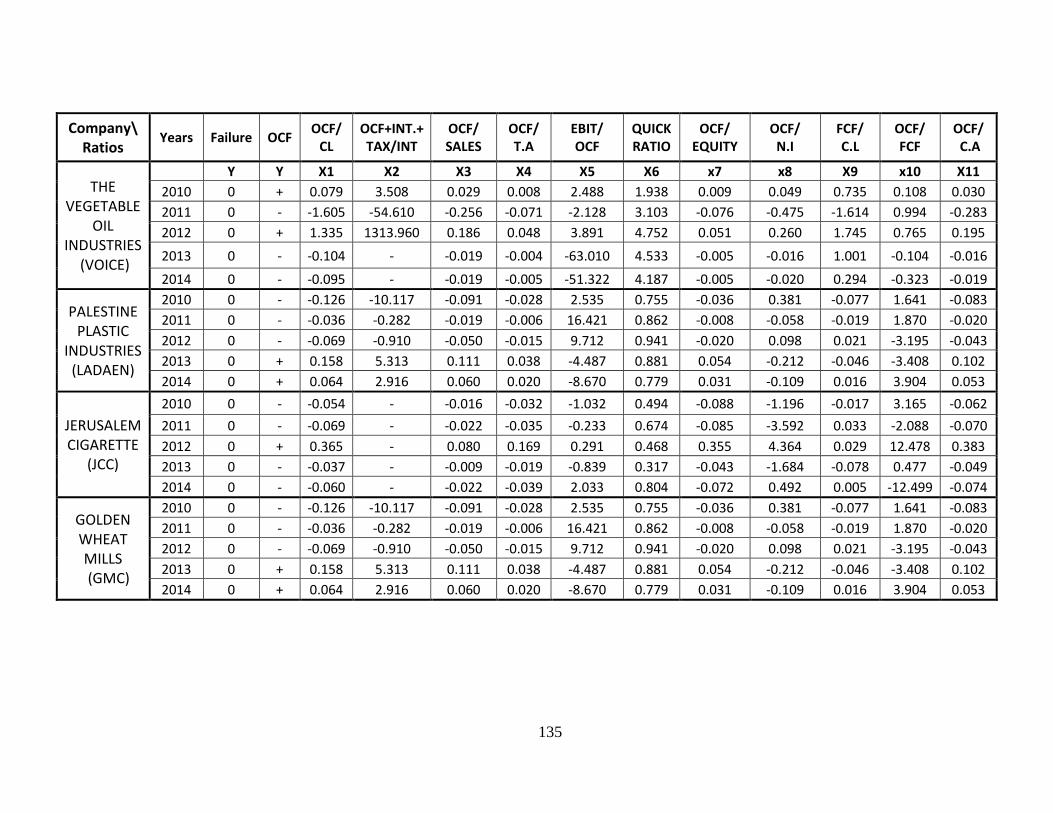
135
Company\ Ratios
Years Failure OCF OCF/
CL OCF+INT.+ TAX/INT
OCF/ SALES
OCF/ T.A
EBIT/ OCF
QUICK RATIO
OCF/ EQUITY
OCF/ N.I
FCF/ C.L
OCF/ FCF
OCF/ C.A
THE VEGETABLE
OIL INDUSTRIES
(VOICE)
Y Y X1 X2 X3 X4 X5 X6 x7 x8 X9 x10 X11
2010 0 + 0.079 3.508 0.029 0.008 2.488 1.938 0.009 0.049 0.735 0.108 0.030
2011 0 - -1.605 -54.610 -0.256 -0.071 -2.128 3.103 -0.076 -0.475 -1.614 0.994 -0.283
2012 0 + 1.335 1313.960 0.186 0.048 3.891 4.752 0.051 0.260 1.745 0.765 0.195
2013 0 - -0.104 - -0.019 -0.004 -63.010 4.533 -0.005 -0.016 1.001 -0.104 -0.016
2014 0 - -0.095 - -0.019 -0.005 -51.322 4.187 -0.005 -0.020 0.294 -0.323 -0.019
PALESTINE PLASTIC
INDUSTRIES (LADAEN)
2010 0 - -0.126 -10.117 -0.091 -0.028 2.535 0.755 -0.036 0.381 -0.077 1.641 -0.083
2011 0 - -0.036 -0.282 -0.019 -0.006 16.421 0.862 -0.008 -0.058 -0.019 1.870 -0.020
2012 0 - -0.069 -0.910 -0.050 -0.015 9.712 0.941 -0.020 0.098 0.021 -3.195 -0.043
2013 0 + 0.158 5.313 0.111 0.038 -4.487 0.881 0.054 -0.212 -0.046 -3.408 0.102
2014 0 + 0.064 2.916 0.060 0.020 -8.670 0.779 0.031 -0.109 0.016 3.904 0.053
JERUSALEM CIGARETTE
(JCC)
2010 0 - -0.054 - -0.016 -0.032 -1.032 0.494 -0.088 -1.196 -0.017 3.165 -0.062
2011 0 - -0.069 - -0.022 -0.035 -0.233 0.674 -0.085 -3.592 0.033 -2.088 -0.070
2012 0 + 0.365 - 0.080 0.169 0.291 0.468 0.355 4.364 0.029 12.478 0.383
2013 0 - -0.037 - -0.009 -0.019 -0.839 0.317 -0.043 -1.684 -0.078 0.477 -0.049
2014 0 - -0.060 - -0.022 -0.039 2.033 0.804 -0.072 0.492 0.005 -12.499 -0.074
GOLDEN WHEAT MILLS
(GMC)
2010 0 - -0.126 -10.117 -0.091 -0.028 2.535 0.755 -0.036 0.381 -0.077 1.641 -0.083
2011 0 - -0.036 -0.282 -0.019 -0.006 16.421 0.862 -0.008 -0.058 -0.019 1.870 -0.020
2012 0 - -0.069 -0.910 -0.050 -0.015 9.712 0.941 -0.020 0.098 0.021 -3.195 -0.043
2013 0 + 0.158 5.313 0.111 0.038 -4.487 0.881 0.054 -0.212 -0.046 -3.408 0.102
2014 0 + 0.064 2.916 0.060 0.020 -8.670 0.779 0.031 -0.109 0.016 3.904 0.053
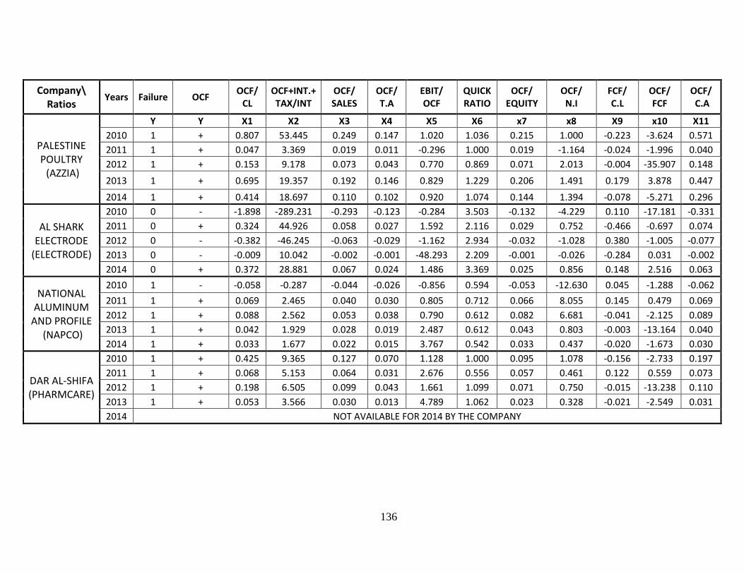
136
Company\ Ratios
Years Failure OCF OCF/
CL OCF+INT.+ TAX/INT
OCF/ SALES
OCF/ T.A
EBIT/ OCF
QUICK RATIO
OCF/ EQUITY
OCF/ N.I
FCF/ C.L
OCF/ FCF
OCF/ C.A
PALESTINE POULTRY (AZZIA)
Y Y X1 X2 X3 X4 X5 X6 x7 x8 X9 x10 X11
2010 1 + 0.807 53.445 0.249 0.147 1.020 1.036 0.215 1.000 -0.223 -3.624 0.571
2011 1 + 0.047 3.369 0.019 0.011 -0.296 1.000 0.019 -1.164 -0.024 -1.996 0.040
2012 1 + 0.153 9.178 0.073 0.043 0.770 0.869 0.071 2.013 -0.004 -35.907 0.148
2013 1 + 0.695 19.357 0.192 0.146 0.829 1.229 0.206 1.491 0.179 3.878 0.447
2014 1 + 0.414 18.697 0.110 0.102 0.920 1.074 0.144 1.394 -0.078 -5.271 0.296
AL SHARK ELECTRODE
(ELECTRODE)
2010 0 - -1.898 -289.231 -0.293 -0.123 -0.284 3.503 -0.132 -4.229 0.110 -17.181 -0.331
2011 0 + 0.324 44.926 0.058 0.027 1.592 2.116 0.029 0.752 -0.466 -0.697 0.074
2012 0 - -0.382 -46.245 -0.063 -0.029 -1.162 2.934 -0.032 -1.028 0.380 -1.005 -0.077
2013 0 - -0.009 10.042 -0.002 -0.001 -48.293 2.209 -0.001 -0.026 -0.284 0.031 -0.002
2014 0 + 0.372 28.881 0.067 0.024 1.486 3.369 0.025 0.856 0.148 2.516 0.063
NATIONAL ALUMINUM
AND PROFILE (NAPCO)
2010 1 - -0.058 -0.287 -0.044 -0.026 -0.856 0.594 -0.053 -12.630 0.045 -1.288 -0.062
2011 1 + 0.069 2.465 0.040 0.030 0.805 0.712 0.066 8.055 0.145 0.479 0.069
2012 1 + 0.088 2.562 0.053 0.038 0.790 0.612 0.082 6.681 -0.041 -2.125 0.089
2013 1 + 0.042 1.929 0.028 0.019 2.487 0.612 0.043 0.803 -0.003 -13.164 0.040
2014 1 + 0.033 1.677 0.022 0.015 3.767 0.542 0.033 0.437 -0.020 -1.673 0.030
DAR AL-SHIFA (PHARMCARE)
2010 1 + 0.425 9.365 0.127 0.070 1.128 1.000 0.095 1.078 -0.156 -2.733 0.197
2011 1 + 0.068 5.153 0.064 0.031 2.676 0.556 0.057 0.461 0.122 0.559 0.073
2012 1 + 0.198 6.505 0.099 0.043 1.661 1.099 0.071 0.750 -0.015 -13.238 0.110
2013 1 + 0.053 3.566 0.030 0.013 4.789 1.062 0.023 0.328 -0.021 -2.549 0.031
2014 NOT AVAILABLE FOR 2014 BY THE COMPANY
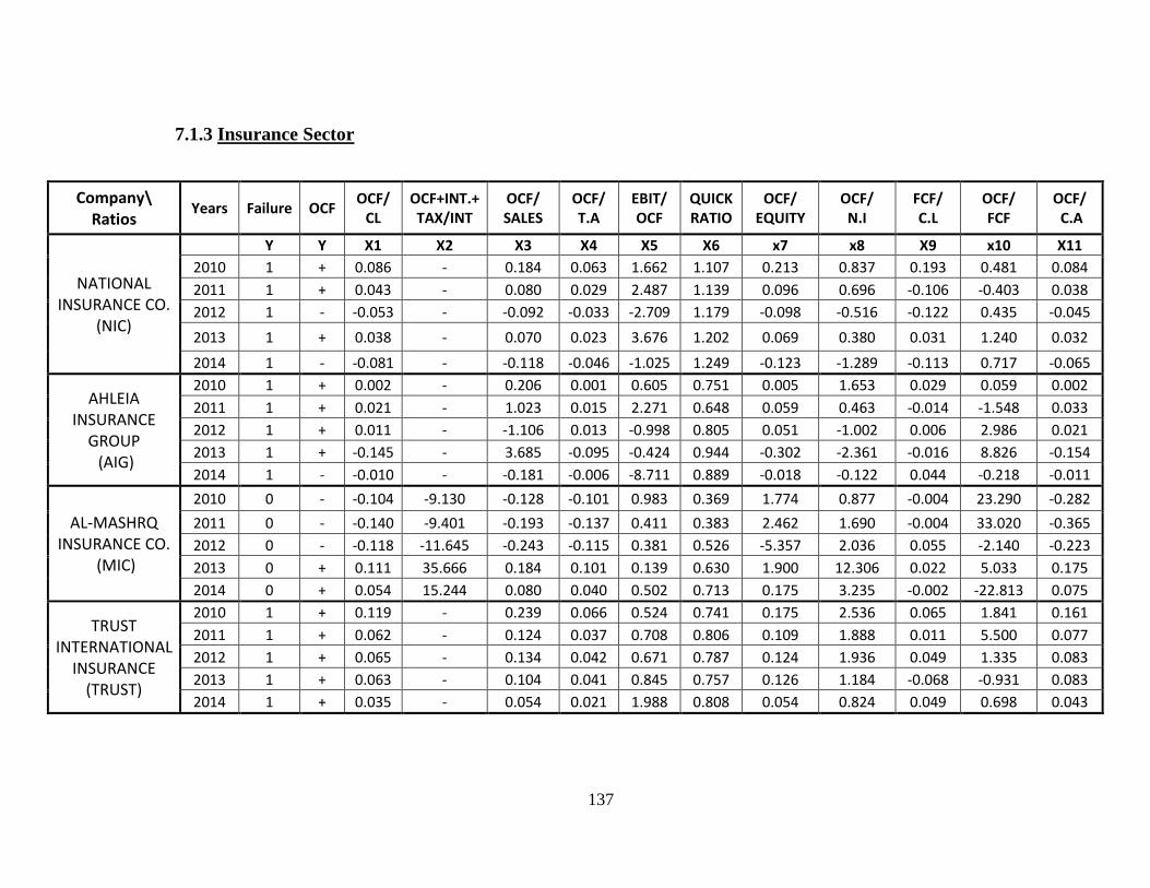
137
7.1.3 Insurance Sector
Company\ Ratios
Years Failure OCF OCF/
CL OCF+INT.+ TAX/INT
OCF/ SALES
OCF/ T.A
EBIT/ OCF
QUICK RATIO
OCF/ EQUITY
OCF/ N.I
FCF/ C.L
OCF/ FCF
OCF/ C.A
NATIONAL INSURANCE CO.
(NIC)
Y Y X1 X2 X3 X4 X5 X6 x7 x8 X9 x10 X11
2010 1 + 0.086 - 0.184 0.063 1.662 1.107 0.213 0.837 0.193 0.481 0.084
2011 1 + 0.043 - 0.080 0.029 2.487 1.139 0.096 0.696 -0.106 -0.403 0.038
2012 1 - -0.053 - -0.092 -0.033 -2.709 1.179 -0.098 -0.516 -0.122 0.435 -0.045
2013 1 + 0.038 - 0.070 0.023 3.676 1.202 0.069 0.380 0.031 1.240 0.032
2014 1 - -0.081 - -0.118 -0.046 -1.025 1.249 -0.123 -1.289 -0.113 0.717 -0.065
AHLEIA INSURANCE
GROUP (AIG)
2010 1 + 0.002 - 0.206 0.001 0.605 0.751 0.005 1.653 0.029 0.059 0.002
2011 1 + 0.021 - 1.023 0.015 2.271 0.648 0.059 0.463 -0.014 -1.548 0.033
2012 1 + 0.011 - -1.106 0.013 -0.998 0.805 0.051 -1.002 0.006 2.986 0.021
2013 1 + -0.145 - 3.685 -0.095 -0.424 0.944 -0.302 -2.361 -0.016 8.826 -0.154
2014 1 - -0.010 - -0.181 -0.006 -8.711 0.889 -0.018 -0.122 0.044 -0.218 -0.011
AL-MASHRQ INSURANCE CO.
(MIC)
2010 0 - -0.104 -9.130 -0.128 -0.101 0.983 0.369 1.774 0.877 -0.004 23.290 -0.282
2011 0 - -0.140 -9.401 -0.193 -0.137 0.411 0.383 2.462 1.690 -0.004 33.020 -0.365
2012 0 - -0.118 -11.645 -0.243 -0.115 0.381 0.526 -5.357 2.036 0.055 -2.140 -0.223
2013 0 + 0.111 35.666 0.184 0.101 0.139 0.630 1.900 12.306 0.022 5.033 0.175
2014 0 + 0.054 15.244 0.080 0.040 0.502 0.713 0.175 3.235 -0.002 -22.813 0.075
TRUST INTERNATIONAL
INSURANCE (TRUST)
2010 1 + 0.119 - 0.239 0.066 0.524 0.741 0.175 2.536 0.065 1.841 0.161
2011 1 + 0.062 - 0.124 0.037 0.708 0.806 0.109 1.888 0.011 5.500 0.077
2012 1 + 0.065 - 0.134 0.042 0.671 0.787 0.124 1.936 0.049 1.335 0.083
2013 1 + 0.063 - 0.104 0.041 0.845 0.757 0.126 1.184 -0.068 -0.931 0.083
2014 1 + 0.035 - 0.054 0.021 1.988 0.808 0.054 0.824 0.049 0.698 0.043
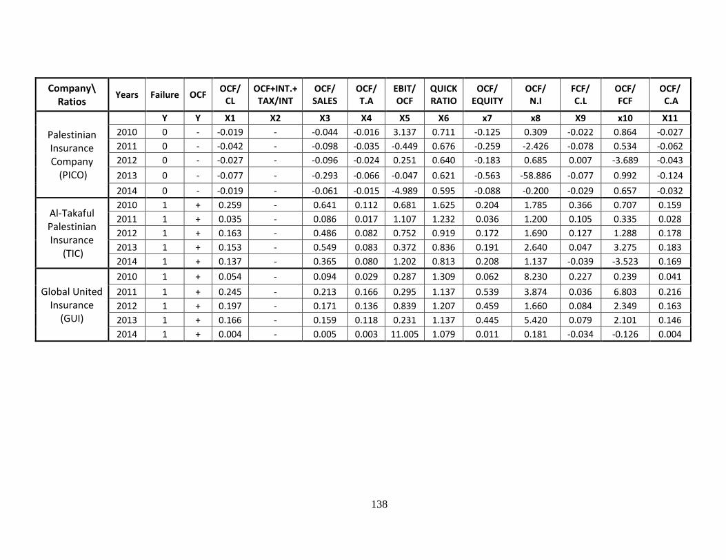
138
Company\ Ratios
Years Failure OCF OCF/
CL OCF+INT.+ TAX/INT
OCF/ SALES
OCF/ T.A
EBIT/ OCF
QUICK RATIO
OCF/ EQUITY
OCF/ N.I
FCF/ C.L
OCF/ FCF
OCF/ C.A
Palestinian Insurance Company
(PICO)
Y Y X1 X2 X3 X4 X5 X6 x7 x8 X9 x10 X11
2010 0 - -0.019 - -0.044 -0.016 3.137 0.711 -0.125 0.309 -0.022 0.864 -0.027
2011 0 - -0.042 - -0.098 -0.035 -0.449 0.676 -0.259 -2.426 -0.078 0.534 -0.062
2012 0 - -0.027 - -0.096 -0.024 0.251 0.640 -0.183 0.685 0.007 -3.689 -0.043
2013 0 - -0.077 - -0.293 -0.066 -0.047 0.621 -0.563 -58.886 -0.077 0.992 -0.124
2014 0 - -0.019 - -0.061 -0.015 -4.989 0.595 -0.088 -0.200 -0.029 0.657 -0.032
Al-Takaful Palestinian Insurance
(TIC)
2010 1 + 0.259 - 0.641 0.112 0.681 1.625 0.204 1.785 0.366 0.707 0.159
2011 1 + 0.035 - 0.086 0.017 1.107 1.232 0.036 1.200 0.105 0.335 0.028
2012 1 + 0.163 - 0.486 0.082 0.752 0.919 0.172 1.690 0.127 1.288 0.178
2013 1 + 0.153 - 0.549 0.083 0.372 0.836 0.191 2.640 0.047 3.275 0.183
2014 1 + 0.137 - 0.365 0.080 1.202 0.813 0.208 1.137 -0.039 -3.523 0.169
Global United Insurance
(GUI)
2010 1 + 0.054 - 0.094 0.029 0.287 1.309 0.062 8.230 0.227 0.239 0.041
2011 1 + 0.245 - 0.213 0.166 0.295 1.137 0.539 3.874 0.036 6.803 0.216
2012 1 + 0.197 - 0.171 0.136 0.839 1.207 0.459 1.660 0.084 2.349 0.163
2013 1 + 0.166 - 0.159 0.118 0.231 1.137 0.445 5.420 0.079 2.101 0.146
2014 1 + 0.004 - 0.005 0.003 11.005 1.079 0.011 0.181 -0.034 -0.126 0.004
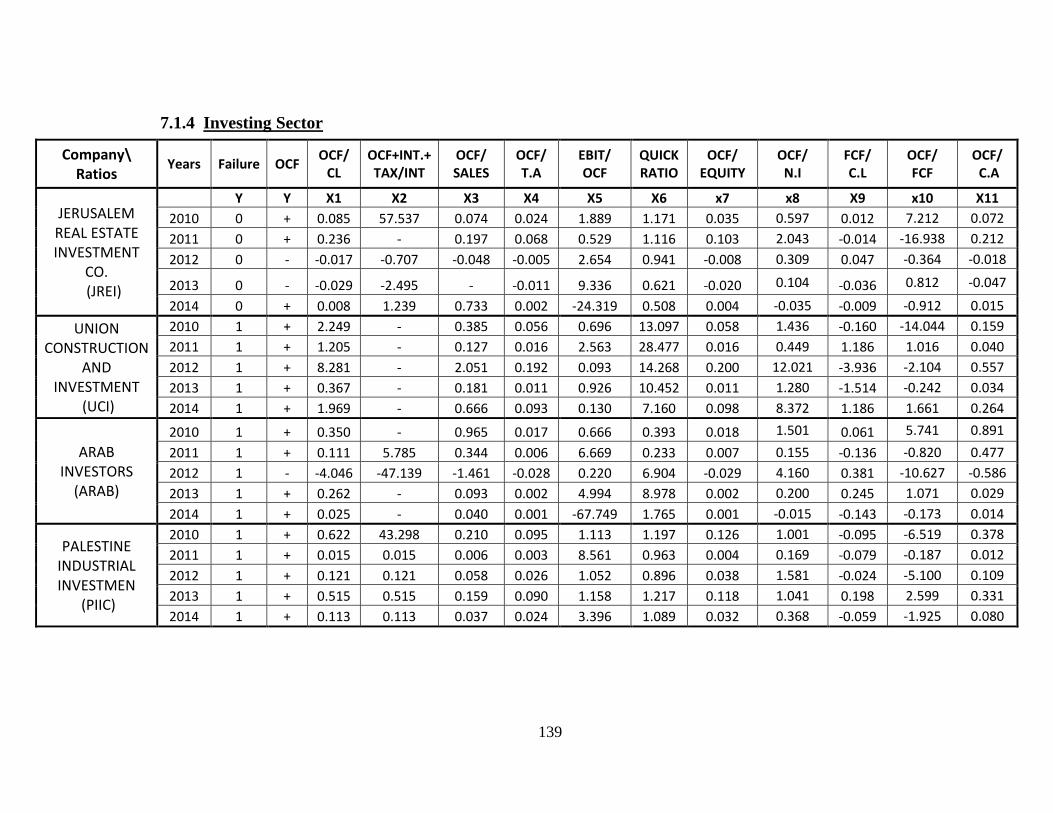
139
7.1.4 Investing Sector
Company\ Ratios
Years Failure OCF OCF/
CL OCF+INT.+ TAX/INT
OCF/ SALES
OCF/ T.A
EBIT/ OCF
QUICK RATIO
OCF/ EQUITY
OCF/ N.I
FCF/ C.L
OCF/ FCF
OCF/ C.A
JERUSALEM REAL ESTATE INVESTMENT
CO. (JREI)
Y Y X1 X2 X3 X4 X5 X6 x7 x8 X9 x10 X11
2010 0 + 0.085 57.537 0.074 0.024 1.889 1.171 0.035 0.597 0.012 7.212 0.072
2011 0 + 0.236 - 0.197 0.068 0.529 1.116 0.103 2.043 -0.014 -16.938 0.212
2012 0 - -0.017 -0.707 -0.048 -0.005 2.654 0.941 -0.008 0.309 0.047 -0.364 -0.018
2013 0 - -0.029 -2.495 - -0.011 9.336 0.621 -0.020 0.104 -0.036 0.812 -0.047
2014 0 + 0.008 1.239 0.733 0.002 -24.319 0.508 0.004 -0.035 -0.009 -0.912 0.015
UNION CONSTRUCTION
AND INVESTMENT
(UCI)
2010 1 + 2.249 - 0.385 0.056 0.696 13.097 0.058 1.436 -0.160 -14.044 0.159
2011 1 + 1.205 - 0.127 0.016 2.563 28.477 0.016 0.449 1.186 1.016 0.040
2012 1 + 8.281 - 2.051 0.192 0.093 14.268 0.200 12.021 -3.936 -2.104 0.557
2013 1 + 0.367 - 0.181 0.011 0.926 10.452 0.011 1.280 -1.514 -0.242 0.034
2014 1 + 1.969 - 0.666 0.093 0.130 7.160 0.098 8.372 1.186 1.661 0.264
ARAB INVESTORS
(ARAB)
2010 1 + 0.350 - 0.965 0.017 0.666 0.393 0.018 1.501 0.061 5.741 0.891
2011 1 + 0.111 5.785 0.344 0.006 6.669 0.233 0.007 0.155 -0.136 -0.820 0.477
2012 1 - -4.046 -47.139 -1.461 -0.028 0.220 6.904 -0.029 4.160 0.381 -10.627 -0.586
2013 1 + 0.262 - 0.093 0.002 4.994 8.978 0.002 0.200 0.245 1.071 0.029
2014 1 + 0.025 - 0.040 0.001 -67.749 1.765 0.001 -0.015 -0.143 -0.173 0.014
PALESTINE INDUSTRIAL INVESTMEN
(PIIC)
2010 1 + 0.622 43.298 0.210 0.095 1.113 1.197 0.126 1.001 -0.095 -6.519 0.378
2011 1 + 0.015 0.015 0.006 0.003 8.561 0.963 0.004 0.169 -0.079 -0.187 0.012
2012 1 + 0.121 0.121 0.058 0.026 1.052 0.896 0.038 1.581 -0.024 -5.100 0.109
2013 1 + 0.515 0.515 0.159 0.090 1.158 1.217 0.118 1.041 0.198 2.599 0.331
2014 1 + 0.113 0.113 0.037 0.024 3.396 1.089 0.032 0.368 -0.059 -1.925 0.080
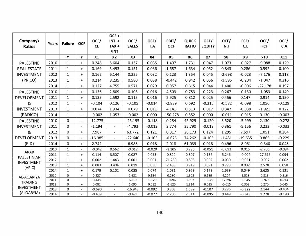
140
Company\ Ratios
Years Failure OCF OCF/
CL
OCF + INT + TAX + /INT
OCF/ SALES
OCF/ T.A
EBIT/ OCF
QUICK RATIO
OCF/ EQUITY
OCF/ N.I
FCF/ C.L
OCF/ FCF
OCF/ C.A
PALESTINE REAL ESTATE INVESTMENT
(PRICO)
Y Y X1 X2 X3 X4 X5 X6 x7 x8 X9 x10 X11
2010 1 + 0.248 5.604 0.137 0.035 1.407 1.731 0.047 1.073 -0.027 -9.088 0.129
2011 1 + 0.169 5.493 0.151 0.036 1.687 1.634 0.052 0.843 0.286 0.592 0.100
2012 1 + 0.162 6.144 0.225 0.032 0.123 1.354 0.045 -2.698 -0.023 -7.176 0.118
2013 1 + 0.214 8.235 0.580 0.038 -0.442 0.942 0.056 -1.595 -0.204 -1.047 0.216
2014 1 + 0.127 4.755 0.571 0.029 0.957 0.615 0.044 1.400 -0.006 -22.178 0.197
PALESTINE DEVELOPMENT
& INVESTMENT
(PADICO)
2010 1 + 0.136 2.809 0.103 0.016 4.503 0.753 0.223 0.267 -0.130 -1.053 0.149
2011 1 + 0.135 2.592 0.115 0.016 2.925 0.812 0.025 0.456 0.147 0.914 0.150
2012 1 - -0.104 0.126 -0.105 -0.014 -2.839 0.692 -0.215 -0.582 -0.098 1.056 -0.129
2013 1 + 0.074 1.934 0.079 0.011 4.141 0.513 0.017 0.347 -0.038 -1.921 0.122
2014 1 - -0.002 1.053 -0.002 0.000 -150.278 0.552 0.000 -0.011 -0.015 0.130 -0.003
PALESTINE INVESTMENT
& DEVELOPMENT
(PID)
2010 0 - -12.775 - -25.195 -0.118 0.284 45.929 -0.120 3.520 -5.999 2.130 -0.278
2011 0 - -1.194 - -4.793 -0.012 2.774 35.790 -0.013 0.361 -5.156 0.232 -0.033
2012 0 + 7.987 - 63.772 0.121 0.817 28.173 0.124 1.295 7.597 1.051 0.284
2013 0 - -16.985 - -22.640 -0.103 -0.675 74.262 -0.105 -1.481 -19.635 0.865 -0.229
2014 0 + 2.742 - 6.985 0.018 2.018 61.039 0.018 0.496 -8.061 -0.340 0.045
ARAB PALESTINIAN INVESTMENT
(APIC)
2010 1 - -0.042 0.562 -0.012 -0.020 -3.105 0.786 -0.051 -0.692 0.015 -2.706 -0.034
2011 1 + 0.114 3.507 0.027 0.053 0.822 0.807 0.136 5.246 -0.004 -27.615 0.094
2012 1 + 0.002 1.443 0.001 0.001 71.280 0.808 0.002 0.030 -0.021 -0.097 0.002
2013 1 + 0.083 3.404 0.019 0.036 2.433 0.919 0.091 0.773 0.032 2.578 0.058
2014 1 + 0.179 5.102 0.035 0.074 1.081 0.959 0.179 1.639 0.049 3.625 0.121
AL-AQARIYA TRADING
INVESTMENT (ALQARYIA)
2010 0 + 0.827 - 2.681 0.154 0.280 1.603 0.189 4.204 1.018 0.813 0.516
2011 0 - -1.419 - -5.152 -0.125 -0.096 1.987 -0.138 -12.292 -1.845 0.769 -0.714
2012 0 + 0.082 - 1.095 0.012 -1.625 1.814 0.015 -0.615 0.303 0.270 0.045
2013 0 - -0.690 - -16.943 -0.092 0.303 1.589 -0.107 3.296 -0.322 2.144 -0.434
2014 0 - -0.439 - -0.471 -0.077 2.205 2.314 -0.095 0.449 -0.343 1.278 -0.190
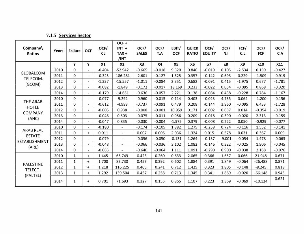
141
7.1.5 Services Sector
Company\ Ratios
Years Failure OCF OCF/
CL
OCF + INT + TAX + /INT
OCF/ SALES
OCF/ T.A
EBIT/ OCF
QUICK RATIO
OCF/ EQUITY
OCF/ N.I
FCF/ C.L
OCF/ FCF
OCF/ C.A
GLOBALCOM TELECOM.
(GCOM)
Y Y X1 X2 X3 X4 X5 X6 x7 x8 X9 x10 X11
2010 0 - -0.404 -52.942 -0.665 -0.018 9.520 0.846 -0.019 0.105 -2.534 0.159 -0.427
2011 0 - -0.325 -186.281 -2.601 -0.127 1.525 0.357 -0.142 0.693 0.229 -1.509 -0.919
2012 0 - -1.337 -15.557 -1.011 -0.084 2.351 0.682 -0.091 0.415 -1.975 0.677 -1.781
2013 0 - -0.082 -1.849 -0.172 -0.017 18.169 0.233 -0.022 0.054 -0.095 0.868 -0.320
2014 0 - -0.179 -14.651 -0.636 -0.057 2.221 0.138 -0.084 0.438 -0.228 0.784 -1.167
THE ARAB HOTLE
COMPANY (AHC)
2010 0 - -0.077 -9.292 -0.960 -0.015 0.114 0.403 -0.023 4.735 0.064 -1.200 -0.156
2011 0 - -0.612 -4.998 -0.737 -0.091 0.479 0.208 -0.144 3.960 -0.095 6.453 -1.728
2012 0 - -0.005 0.938 -0.008 -0.001 10.959 0.171 -0.002 0.037 0.014 -0.354 -0.019
2013 0 - -0.046 0.503 -0.075 -0.011 0.956 0.209 -0.018 0.390 -0.020 2.313 -0.159
2014 0 - -0.047 0.835 -0.030 -0.004 -1.575 0.379 -0.008 0.222 0.050 -0.929 -0.077
ARAB REAL ESTATE
ESTABLISHMENT (ARE)
2010 0 - -0.180 - -0.174 -0.105 1.382 1.275 -0.258 0.724 -0.116 1.552 -0.141
2011 0 + 0.011 - 0.007 0.006 2.036 1.324 0.015 0.578 0.031 0.367 0.009
2012 0 - -0.079 - -0.056 -0.050 -0.131 1.264 -0.137 -9.001 -0.054 1.478 -0.063
2013 0 - -0.048 - -0.066 -0.036 3.102 1.082 -0.146 0.322 -0.025 1.906 -0.045
2014 0 - -0.083 - -0.646 -0.064 1.111 1.091 -0.290 0.900 -0.038 2.188 -0.076
PALESTINE TELECO. (PALTEL)
2010 1 + 1.445 65.749 0.423 0.260 0.633 2.065 0.366 1.657 0.066 21.948 0.671
2011 1 + 1.700 83.730 0.453 0.292 0.602 1.884 0.391 1.849 -0.064 -26.488 0.871
2012 1 + 1.218 116.225 0.405 0.241 0.712 1.425 0.323 1.805 -0.148 -8.245 0.813
2013 1 + 1.292 139.504 0.457 0.258 0.713 1.345 0.341 1.869 -0.020 -66.148 0.945
2014 1 + 0.701 71.693 0.327 0.155 0.865 1.107 0.223 1.369 -0.069 -10.124 0.621
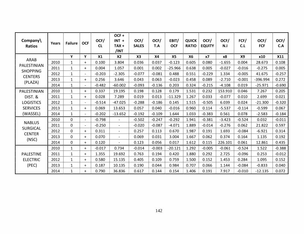
142
Company\ Ratios
Years Failure OCF OCF/
CL
OCF + INT + TAX + /INT
OCF/ SALES
OCF/ T.A
EBIT/ OCF
QUICK RATIO
OCF/ EQUITY
OCF/ N.I
FCF/ C.L
OCF/ FCF
OCF/ C.A
ARAB PALESTINIAN
SHOPPING CENTERS (PLAZA)
Y Y X1 X2 X3 X4 X5 X6 x7 x8 X9 x10 X11
2010 1 + 0.100 3.804 0.036 0.037 -0.123 0.605 0.080 -1.655 0.004 28.673 0.108
2011 1 + 0.004 1.057 0.001 0.002 -25.966 0.638 0.005 -0.027 -0.016 -0.275 0.005
2012 1 - -0.203 -2.305 -0.077 -0.081 0.488 0.551 -0.229 1.334 -0.005 41.675 -0.257
2013 1 + 0.256 3.646 0.043 0.063 -0.023 0.458 0.089 -2.710 -0.001 -396.994 0.272
2014 1 - -0.482 -60.002 -0.093 -0.136 0.203 0.324 -0.215 -4.108 0.019 -25.971 -0.690
PALESTINIAN DIST. &
LOGISTICS SERVICES (WASSEL)
2010 1 + 0.337 19.195 0.198 0.128 0.179 1.531 0.232 153.910 0.046 7.267 0.205
2011 1 + 0.028 7.289 0.019 0.013 -11.329 1.267 0.033 -0.077 0.010 2.699 0.021
2012 1 - -0.514 -47.025 -0.288 -0.186 0.145 1.515 -0.505 6.039 0.024 -21.300 -0.320
2013 1 + 0.069 13.653 0.057 0.040 -0.016 0.960 0.114 -5.537 -0.114 -0.599 0.067
2014 1 - -0.202 -13.652 -0.192 -0.109 1.644 1.033 -0.383 0.561 0.078 -2.583 -0.184
NABLUS SURGICAL CENTER (NSC)
2010 0 - -0.798 - -0.502 -0.247 -0.292 1.941 -0.381 -3.423 -0.524 0.032 -0.011
2011 0 - -0.250 - -0.020 -0.087 -4.071 1.889 -0.014 -0.276 0.062 21.822 0.597
2012 0 + 0.311 - 0.257 0.113 0.670 1.987 0.191 1.693 -0.084 -6.921 0.314
2013 0 + 0.070 - 0.069 0.031 3.004 1.667 0.062 0.374 0.164 1.135 0.192
2014 0 + 0.120 - 0.123 0.056 0.017 1.612 0.115 226.101 0.061 12.861 0.435
PALESTINE ELECTRIC
(PEC)
2010 1 + -0.017 0.734 -0.014 -0.003 -20.121 1.292 -0.005 -0.061 -0.524 1.522 -0.388
2011 1 + 1.355 19.692 0.763 0.194 0.420 1.880 0.292 2.725 -0.096 0.253 -0.012
2012 1 + 0.580 15.135 0.405 0.109 0.759 1.500 0.152 1.453 0.284 1.095 0.152
2013 1 + 0.187 10.135 0.190 0.044 0.984 0.707 0.066 1.144 -0.084 -0.833 0.040
2014 1 + 0.790 36.836 0.617 0.144 0.154 1.406 0.191 7.917 -0.010 -12.135 0.072
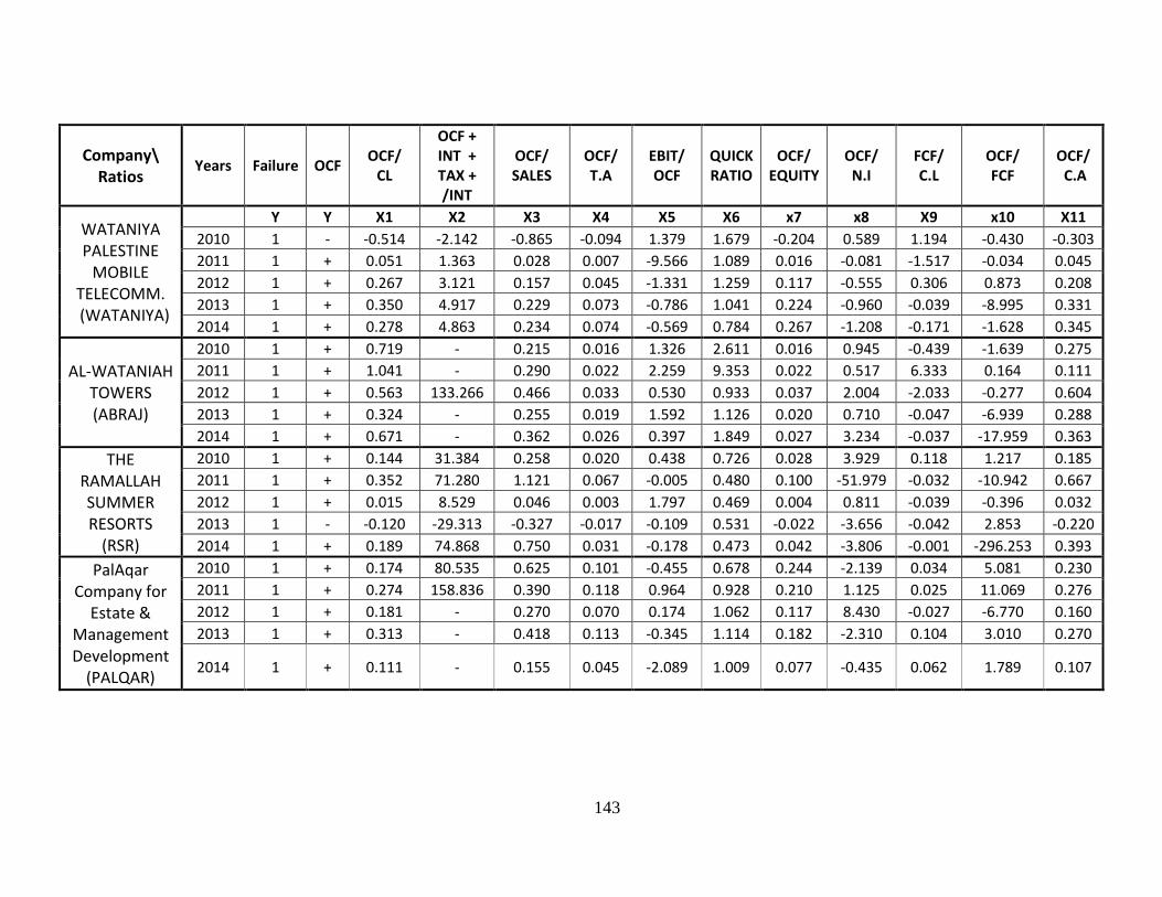
143
Company\ Ratios
Years Failure OCF OCF/
CL
OCF + INT + TAX + /INT
OCF/ SALES
OCF/ T.A
EBIT/ OCF
QUICK RATIO
OCF/ EQUITY
OCF/ N.I
FCF/ C.L
OCF/ FCF
OCF/ C.A
WATANIYA PALESTINE
MOBILE TELECOMM.
(WATANIYA)
Y Y X1 X2 X3 X4 X5 X6 x7 x8 X9 x10 X11
2010 1 - -0.514 -2.142 -0.865 -0.094 1.379 1.679 -0.204 0.589 1.194 -0.430 -0.303
2011 1 + 0.051 1.363 0.028 0.007 -9.566 1.089 0.016 -0.081 -1.517 -0.034 0.045
2012 1 + 0.267 3.121 0.157 0.045 -1.331 1.259 0.117 -0.555 0.306 0.873 0.208
2013 1 + 0.350 4.917 0.229 0.073 -0.786 1.041 0.224 -0.960 -0.039 -8.995 0.331
2014 1 + 0.278 4.863 0.234 0.074 -0.569 0.784 0.267 -1.208 -0.171 -1.628 0.345
AL-WATANIAH TOWERS (ABRAJ)
2010 1 + 0.719 - 0.215 0.016 1.326 2.611 0.016 0.945 -0.439 -1.639 0.275
2011 1 + 1.041 - 0.290 0.022 2.259 9.353 0.022 0.517 6.333 0.164 0.111
2012 1 + 0.563 133.266 0.466 0.033 0.530 0.933 0.037 2.004 -2.033 -0.277 0.604
2013 1 + 0.324 - 0.255 0.019 1.592 1.126 0.020 0.710 -0.047 -6.939 0.288
2014 1 + 0.671 - 0.362 0.026 0.397 1.849 0.027 3.234 -0.037 -17.959 0.363
THE RAMALLAH SUMMER RESORTS
(RSR)
2010 1 + 0.144 31.384 0.258 0.020 0.438 0.726 0.028 3.929 0.118 1.217 0.185
2011 1 + 0.352 71.280 1.121 0.067 -0.005 0.480 0.100 -51.979 -0.032 -10.942 0.667
2012 1 + 0.015 8.529 0.046 0.003 1.797 0.469 0.004 0.811 -0.039 -0.396 0.032
2013 1 - -0.120 -29.313 -0.327 -0.017 -0.109 0.531 -0.022 -3.656 -0.042 2.853 -0.220
2014 1 + 0.189 74.868 0.750 0.031 -0.178 0.473 0.042 -3.806 -0.001 -296.253 0.393
PalAqar Company for
Estate & Management Development
(PALQAR)
2010 1 + 0.174 80.535 0.625 0.101 -0.455 0.678 0.244 -2.139 0.034 5.081 0.230
2011 1 + 0.274 158.836 0.390 0.118 0.964 0.928 0.210 1.125 0.025 11.069 0.276
2012 1 + 0.181 - 0.270 0.070 0.174 1.062 0.117 8.430 -0.027 -6.770 0.160
2013 1 + 0.313 - 0.418 0.113 -0.345 1.114 0.182 -2.310 0.104 3.010 0.270
2014 1 + 0.111 - 0.155 0.045 -2.089 1.009 0.077 -0.435 0.062 1.789 0.107
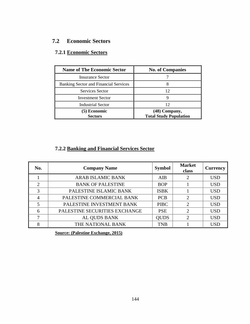
144
7.2 Economic Sectors
7.2.1 Economic Sectors
Name of The Economic Sector No. of Companies
Insurance Sector 7
Banking Sector and Financial Services 8
Services Sector 12
Investment Sector 9
Industrial Sector 12
(5) Economic
Sectors
(48) Company,
Total Study Population
7.2.2 Banking and Financial Services Sector
No. Company Name Symbol Market
class Currency
1 ARAB ISLAMIC BANK AIB 2 USD
2 BANK OF PALESTINE BOP 1 USD
3 PALESTINE ISLAMIC BANK ISBK 1 USD
4 PALESTINE COMMERCIAL BANK PCB 2 USD
5 PALESTINE INVESTMENT BANK PIBC 2 USD
6 PALESTINE SECURITIES EXCHANGE PSE 2 USD
7 AL QUDS BANK QUDS 2 USD
8 THE NATIONAL BANK TNB 1 USD
Source: (Palestine Exchange, 2015)
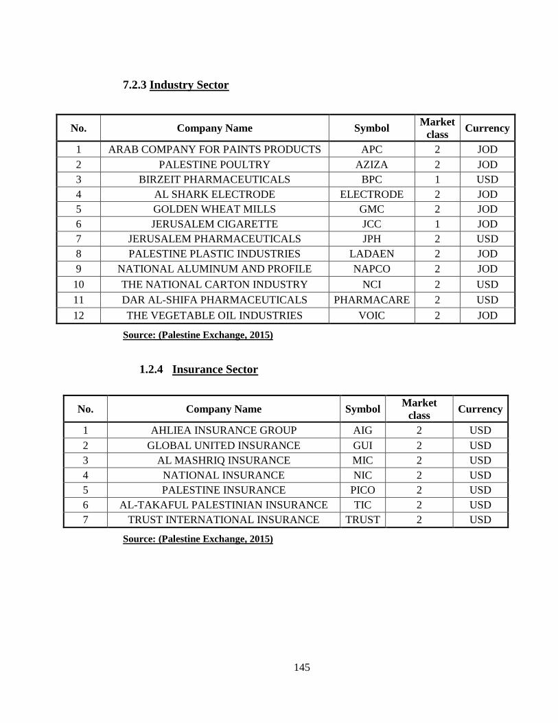
145
7.2.3 Industry Sector
No. Company Name Symbol Market
class Currency
1 ARAB COMPANY FOR PAINTS PRODUCTS APC 2 JOD
2 PALESTINE POULTRY AZIZA 2 JOD
3 BIRZEIT PHARMACEUTICALS BPC 1 USD
4 AL SHARK ELECTRODE ELECTRODE 2 JOD
5 GOLDEN WHEAT MILLS GMC 2 JOD
6 JERUSALEM CIGARETTE JCC 1 JOD
7 JERUSALEM PHARMACEUTICALS JPH 2 USD
8 PALESTINE PLASTIC INDUSTRIES LADAEN 2 JOD
9 NATIONAL ALUMINUM AND PROFILE NAPCO 2 JOD
10 THE NATIONAL CARTON INDUSTRY NCI 2 USD
11 DAR AL-SHIFA PHARMACEUTICALS PHARMACARE 2 USD
12 THE VEGETABLE OIL INDUSTRIES VOIC 2 JOD
Source: (Palestine Exchange, 2015)
1.2.4 Insurance Sector
No. Company Name Symbol Market
class Currency
1 AHLIEA INSURANCE GROUP AIG 2 USD
2 GLOBAL UNITED INSURANCE GUI 2 USD
3 AL MASHRIQ INSURANCE MIC 2 USD
4 NATIONAL INSURANCE NIC 2 USD
5 PALESTINE INSURANCE PICO 2 USD
6 AL-TAKAFUL PALESTINIAN INSURANCE TIC 2 USD
7 TRUST INTERNATIONAL INSURANCE TRUST 2 USD
Source: (Palestine Exchange, 2015)
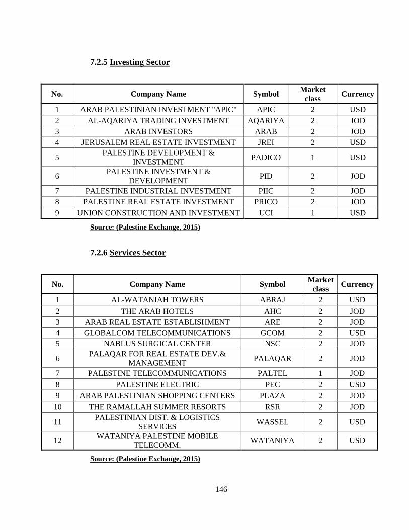
146
7.2.5 Investing Sector
No. Company Name Symbol Market
class Currency
1 ARAB PALESTINIAN INVESTMENT "APIC" APIC 2 USD
2 AL-AQARIYA TRADING INVESTMENT AQARIYA 2 JOD
3 ARAB INVESTORS ARAB 2 JOD
4 JERUSALEM REAL ESTATE INVESTMENT JREI 2 USD
5 PALESTINE DEVELOPMENT &
INVESTMENT PADICO 1 USD
6 PALESTINE INVESTMENT &
DEVELOPMENT PID 2 JOD
7 PALESTINE INDUSTRIAL INVESTMENT PIIC 2 JOD
8 PALESTINE REAL ESTATE INVESTMENT PRICO 2 JOD
9 UNION CONSTRUCTION AND INVESTMENT UCI 1 USD
Source: (Palestine Exchange, 2015)
7.2.6 Services Sector
No. Company Name Symbol Market
class Currency
1 AL-WATANIAH TOWERS ABRAJ 2 USD
2 THE ARAB HOTELS AHC 2 JOD
3 ARAB REAL ESTATE ESTABLISHMENT ARE 2 JOD
4 GLOBALCOM TELECOMMUNICATIONS GCOM 2 USD
5 NABLUS SURGICAL CENTER NSC 2 JOD
6 PALAQAR FOR REAL ESTATE DEV.&
MANAGEMENT PALAQAR 2 JOD
7 PALESTINE TELECOMMUNICATIONS PALTEL 1 JOD
8 PALESTINE ELECTRIC PEC 2 USD
9 ARAB PALESTINIAN SHOPPING CENTERS PLAZA 2 JOD
10 THE RAMALLAH SUMMER RESORTS RSR 2 JOD
11 PALESTINIAN DIST. & LOGISTICS
SERVICES WASSEL 2 USD
12 WATANIYA PALESTINE MOBILE
TELECOMM. WATANIYA 2 USD
Source: (Palestine Exchange, 2015)
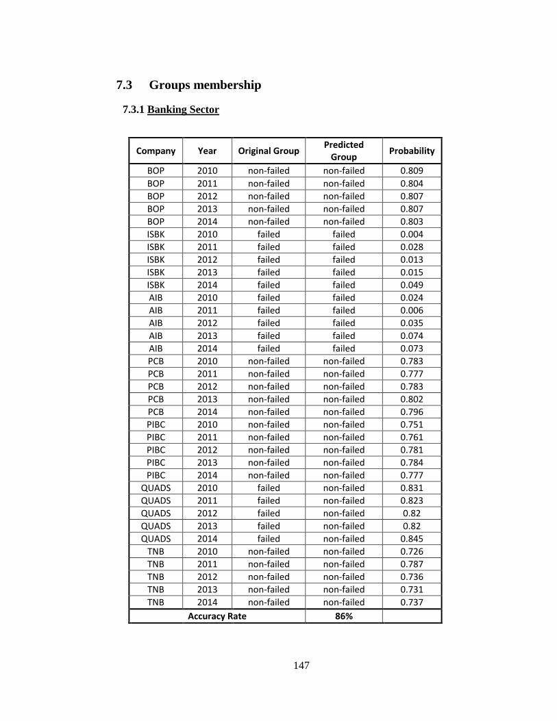
147
7.3 Groups membership
7.3.1 Banking Sector
Company Year Original Group Predicted
Group Probability
BOP 2010 non-failed non-failed 0.809
BOP 2011 non-failed non-failed 0.804
BOP 2012 non-failed non-failed 0.807
BOP 2013 non-failed non-failed 0.807
BOP 2014 non-failed non-failed 0.803
ISBK 2010 failed failed 0.004
ISBK 2011 failed failed 0.028
ISBK 2012 failed failed 0.013
ISBK 2013 failed failed 0.015
ISBK 2014 failed failed 0.049
AIB 2010 failed failed 0.024
AIB 2011 failed failed 0.006
AIB 2012 failed failed 0.035
AIB 2013 failed failed 0.074
AIB 2014 failed failed 0.073
PCB 2010 non-failed non-failed 0.783
PCB 2011 non-failed non-failed 0.777
PCB 2012 non-failed non-failed 0.783
PCB 2013 non-failed non-failed 0.802
PCB 2014 non-failed non-failed 0.796
PIBC 2010 non-failed non-failed 0.751
PIBC 2011 non-failed non-failed 0.761
PIBC 2012 non-failed non-failed 0.781
PIBC 2013 non-failed non-failed 0.784
PIBC 2014 non-failed non-failed 0.777
QUADS 2010 failed non-failed 0.831
QUADS 2011 failed non-failed 0.823
QUADS 2012 failed non-failed 0.82
QUADS 2013 failed non-failed 0.82
QUADS 2014 failed non-failed 0.845
TNB 2010 non-failed non-failed 0.726
TNB 2011 non-failed non-failed 0.787
TNB 2012 non-failed non-failed 0.736
TNB 2013 non-failed non-failed 0.731
TNB 2014 non-failed non-failed 0.737
Accuracy Rate 86%
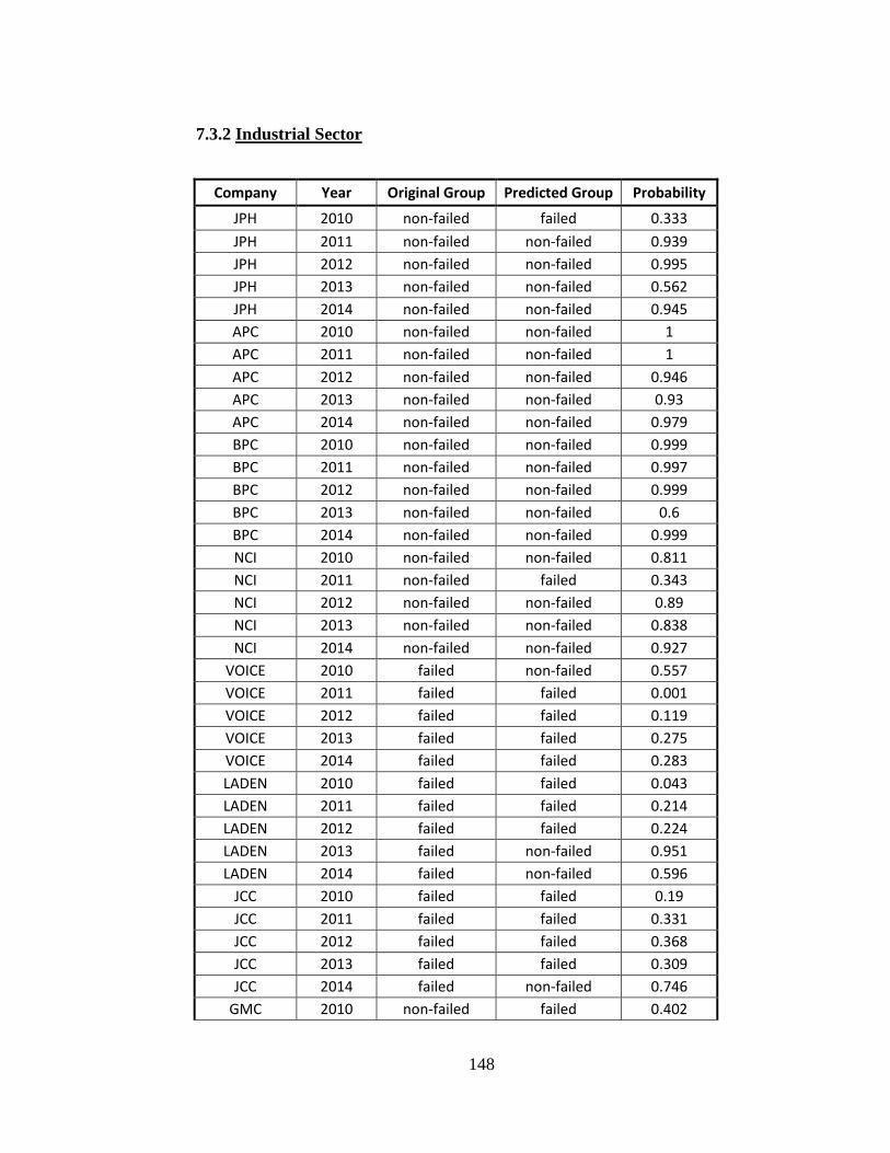
148
7.3.2 Industrial Sector
Company Year Original Group Predicted Group Probability
JPH 2010 non-failed failed 0.333
JPH 2011 non-failed non-failed 0.939
JPH 2012 non-failed non-failed 0.995
JPH 2013 non-failed non-failed 0.562
JPH 2014 non-failed non-failed 0.945
APC 2010 non-failed non-failed 1
APC 2011 non-failed non-failed 1
APC 2012 non-failed non-failed 0.946
APC 2013 non-failed non-failed 0.93
APC 2014 non-failed non-failed 0.979
BPC 2010 non-failed non-failed 0.999
BPC 2011 non-failed non-failed 0.997
BPC 2012 non-failed non-failed 0.999
BPC 2013 non-failed non-failed 0.6
BPC 2014 non-failed non-failed 0.999
NCI 2010 non-failed non-failed 0.811
NCI 2011 non-failed failed 0.343
NCI 2012 non-failed non-failed 0.89
NCI 2013 non-failed non-failed 0.838
NCI 2014 non-failed non-failed 0.927
VOICE 2010 failed non-failed 0.557
VOICE 2011 failed failed 0.001
VOICE 2012 failed failed 0.119
VOICE 2013 failed failed 0.275
VOICE 2014 failed failed 0.283
LADEN 2010 failed failed 0.043
LADEN 2011 failed failed 0.214
LADEN 2012 failed failed 0.224
LADEN 2013 failed non-failed 0.951
LADEN 2014 failed non-failed 0.596
JCC 2010 failed failed 0.19
JCC 2011 failed failed 0.331
JCC 2012 failed failed 0.368
JCC 2013 failed failed 0.309
JCC 2014 failed non-failed 0.746
GMC 2010 non-failed failed 0.402
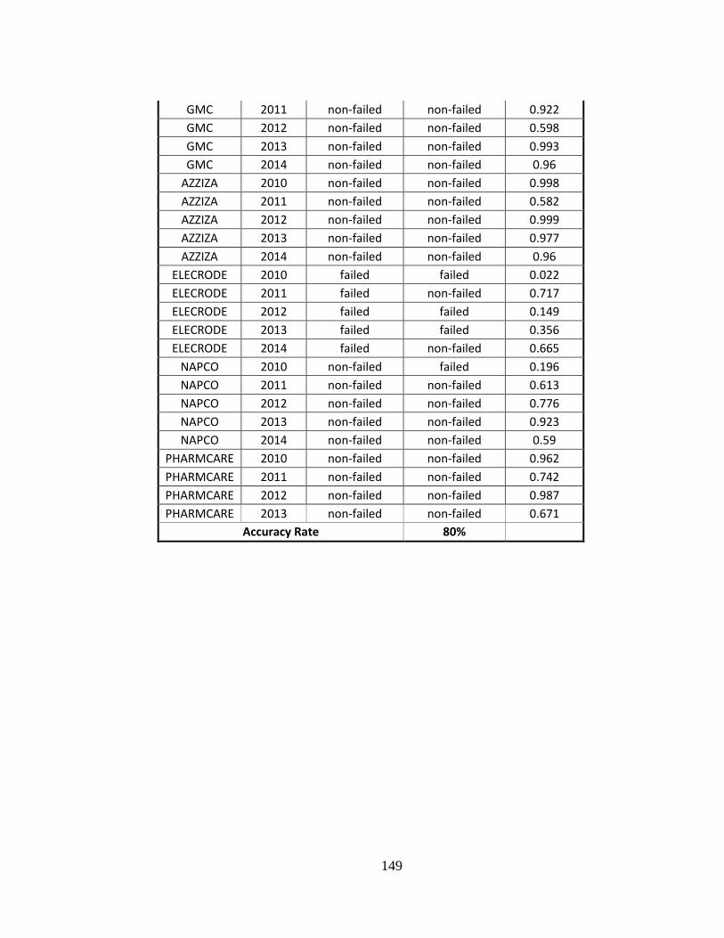
149
GMC 2011 non-failed non-failed 0.922
GMC 2012 non-failed non-failed 0.598
GMC 2013 non-failed non-failed 0.993
GMC 2014 non-failed non-failed 0.96
AZZIZA 2010 non-failed non-failed 0.998
AZZIZA 2011 non-failed non-failed 0.582
AZZIZA 2012 non-failed non-failed 0.999
AZZIZA 2013 non-failed non-failed 0.977
AZZIZA 2014 non-failed non-failed 0.96
ELECRODE 2010 failed failed 0.022
ELECRODE 2011 failed non-failed 0.717
ELECRODE 2012 failed failed 0.149
ELECRODE 2013 failed failed 0.356
ELECRODE 2014 failed non-failed 0.665
NAPCO 2010 non-failed failed 0.196
NAPCO 2011 non-failed non-failed 0.613
NAPCO 2012 non-failed non-failed 0.776
NAPCO 2013 non-failed non-failed 0.923
NAPCO 2014 non-failed non-failed 0.59
PHARMCARE 2010 non-failed non-failed 0.962
PHARMCARE 2011 non-failed non-failed 0.742
PHARMCARE 2012 non-failed non-failed 0.987
PHARMCARE 2013 non-failed non-failed 0.671
Accuracy Rate 80%
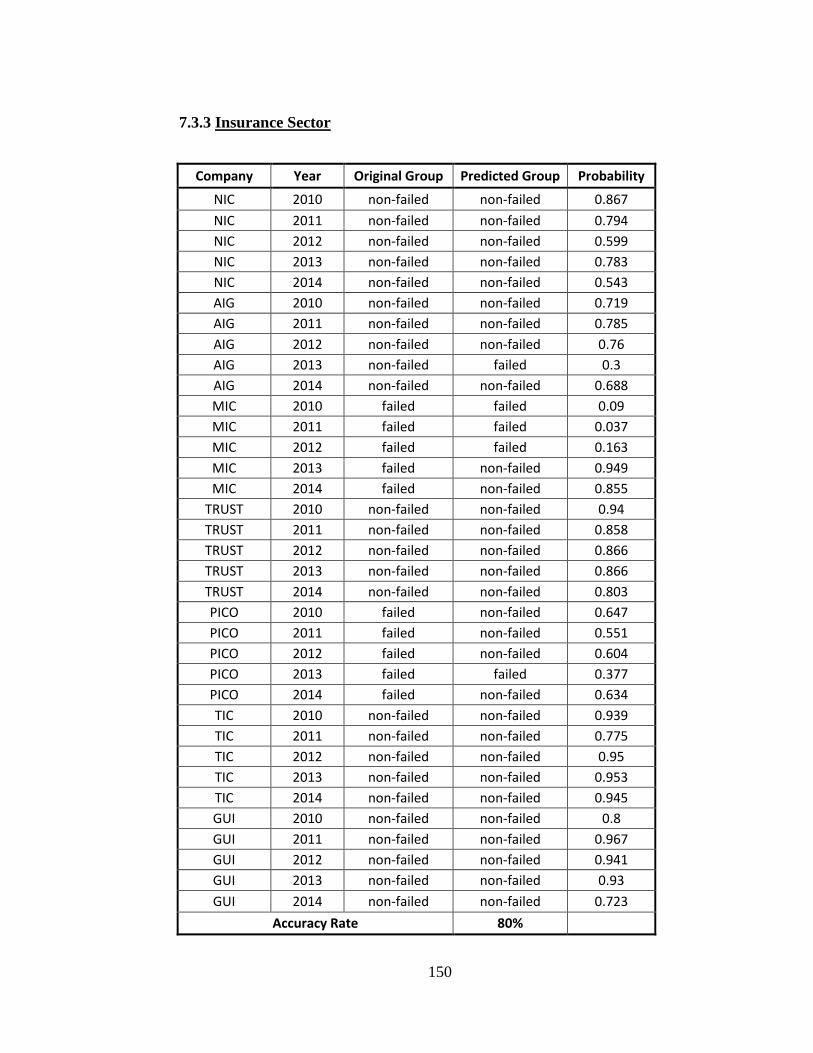
150
7.3.3 Insurance Sector
Company Year Original Group Predicted Group Probability
NIC 2010 non-failed non-failed 0.867
NIC 2011 non-failed non-failed 0.794
NIC 2012 non-failed non-failed 0.599
NIC 2013 non-failed non-failed 0.783
NIC 2014 non-failed non-failed 0.543
AIG 2010 non-failed non-failed 0.719
AIG 2011 non-failed non-failed 0.785
AIG 2012 non-failed non-failed 0.76
AIG 2013 non-failed failed 0.3
AIG 2014 non-failed non-failed 0.688
MIC 2010 failed failed 0.09
MIC 2011 failed failed 0.037
MIC 2012 failed failed 0.163
MIC 2013 failed non-failed 0.949
MIC 2014 failed non-failed 0.855
TRUST 2010 non-failed non-failed 0.94
TRUST 2011 non-failed non-failed 0.858
TRUST 2012 non-failed non-failed 0.866
TRUST 2013 non-failed non-failed 0.866
TRUST 2014 non-failed non-failed 0.803
PICO 2010 failed non-failed 0.647
PICO 2011 failed non-failed 0.551
PICO 2012 failed non-failed 0.604
PICO 2013 failed failed 0.377
PICO 2014 failed non-failed 0.634
TIC 2010 non-failed non-failed 0.939
TIC 2011 non-failed non-failed 0.775
TIC 2012 non-failed non-failed 0.95
TIC 2013 non-failed non-failed 0.953
TIC 2014 non-failed non-failed 0.945
GUI 2010 non-failed non-failed 0.8
GUI 2011 non-failed non-failed 0.967
GUI 2012 non-failed non-failed 0.941
GUI 2013 non-failed non-failed 0.93
GUI 2014 non-failed non-failed 0.723
Accuracy Rate 80%
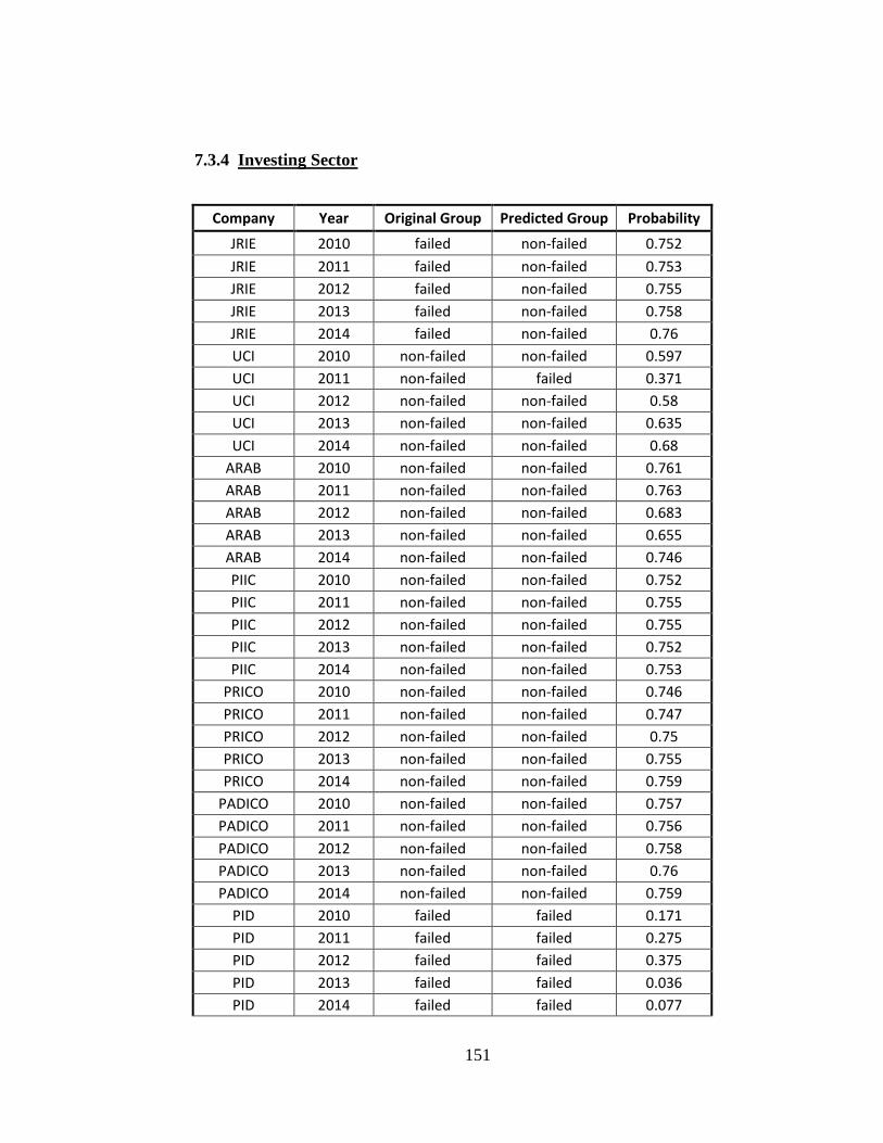
151
7.3.4 Investing Sector
Company Year Original Group Predicted Group Probability
JRIE 2010 failed non-failed 0.752
JRIE 2011 failed non-failed 0.753
JRIE 2012 failed non-failed 0.755
JRIE 2013 failed non-failed 0.758
JRIE 2014 failed non-failed 0.76
UCI 2010 non-failed non-failed 0.597
UCI 2011 non-failed failed 0.371
UCI 2012 non-failed non-failed 0.58
UCI 2013 non-failed non-failed 0.635
UCI 2014 non-failed non-failed 0.68
ARAB 2010 non-failed non-failed 0.761
ARAB 2011 non-failed non-failed 0.763
ARAB 2012 non-failed non-failed 0.683
ARAB 2013 non-failed non-failed 0.655
ARAB 2014 non-failed non-failed 0.746
PIIC 2010 non-failed non-failed 0.752
PIIC 2011 non-failed non-failed 0.755
PIIC 2012 non-failed non-failed 0.755
PIIC 2013 non-failed non-failed 0.752
PIIC 2014 non-failed non-failed 0.753
PRICO 2010 non-failed non-failed 0.746
PRICO 2011 non-failed non-failed 0.747
PRICO 2012 non-failed non-failed 0.75
PRICO 2013 non-failed non-failed 0.755
PRICO 2014 non-failed non-failed 0.759
PADICO 2010 non-failed non-failed 0.757
PADICO 2011 non-failed non-failed 0.756
PADICO 2012 non-failed non-failed 0.758
PADICO 2013 non-failed non-failed 0.76
PADICO 2014 non-failed non-failed 0.759
PID 2010 failed failed 0.171
PID 2011 failed failed 0.275
PID 2012 failed failed 0.375
PID 2013 failed failed 0.036
PID 2014 failed failed 0.077
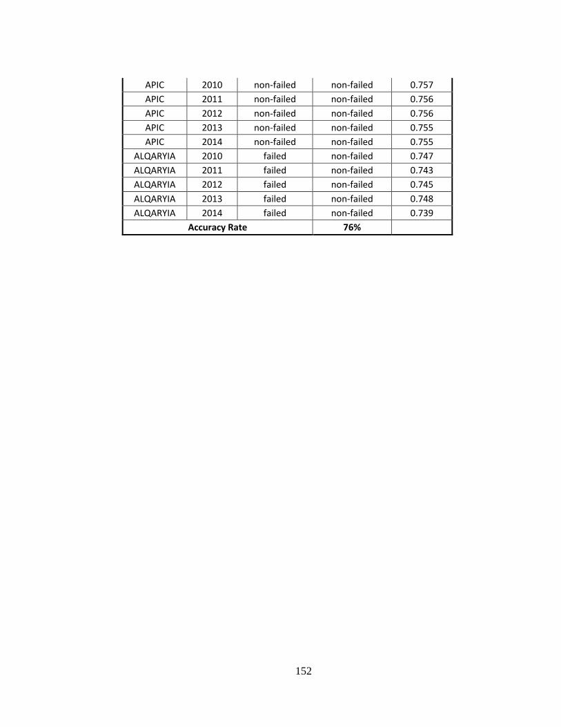
152
APIC 2010 non-failed non-failed 0.757
APIC 2011 non-failed non-failed 0.756
APIC 2012 non-failed non-failed 0.756
APIC 2013 non-failed non-failed 0.755
APIC 2014 non-failed non-failed 0.755
ALQARYIA 2010 failed non-failed 0.747
ALQARYIA 2011 failed non-failed 0.743
ALQARYIA 2012 failed non-failed 0.745
ALQARYIA 2013 failed non-failed 0.748
ALQARYIA 2014 failed non-failed 0.739
Accuracy Rate 76%
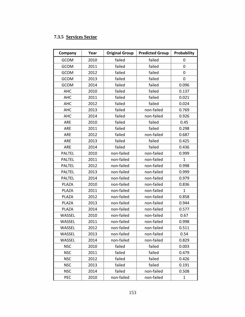
153
7.3.5 Services Sector
Company Year Original Group Predicted Group Probability
GCOM 2010 failed failed 0
GCOM 2011 failed failed 0
GCOM 2012 failed failed 0
GCOM 2013 failed failed 0
GCOM 2014 failed failed 0.096
AHC 2010 failed failed 0.137
AHC 2011 failed failed 0.021
AHC 2012 failed failed 0.024
AHC 2013 failed non-failed 0.769
AHC 2014 failed non-failed 0.926
ARE 2010 failed failed 0.45
ARE 2011 failed failed 0.298
ARE 2012 failed non-failed 0.687
ARE 2013 failed failed 0.425
ARE 2014 failed failed 0.436
PALTEL 2010 non-failed non-failed 0.999
PALTEL 2011 non-failed non-failed 1
PALTEL 2012 non-failed non-failed 0.998
PALTEL 2013 non-failed non-failed 0.999
PALTEL 2014 non-failed non-failed 0.979
PLAZA 2010 non-failed non-failed 0.836
PLAZA 2011 non-failed non-failed 1
PLAZA 2012 non-failed non-failed 0.858
PLAZA 2013 non-failed non-failed 0.944
PLAZA 2014 non-failed non-failed 0.577
WASSEL 2010 non-failed non-failed 0.67
WASSEL 2011 non-failed non-failed 0.998
WASSEL 2012 non-failed non-failed 0.511
WASSEL 2013 non-failed non-failed 0.54
WASSEL 2014 non-failed non-failed 0.829
NSC 2010 failed failed 0.003
NSC 2011 failed failed 0.479
NSC 2012 failed failed 0.426
NSC 2013 failed failed 0.191
NSC 2014 failed non-failed 0.508
PEC 2010 non-failed non-failed 1
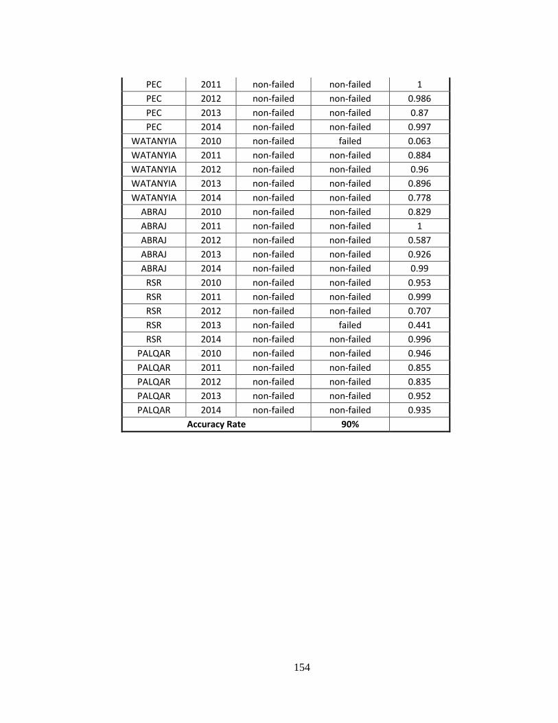
154
PEC 2011 non-failed non-failed 1
PEC 2012 non-failed non-failed 0.986
PEC 2013 non-failed non-failed 0.87
PEC 2014 non-failed non-failed 0.997
WATANYIA 2010 non-failed failed 0.063
WATANYIA 2011 non-failed non-failed 0.884
WATANYIA 2012 non-failed non-failed 0.96
WATANYIA 2013 non-failed non-failed 0.896
WATANYIA 2014 non-failed non-failed 0.778
ABRAJ 2010 non-failed non-failed 0.829
ABRAJ 2011 non-failed non-failed 1
ABRAJ 2012 non-failed non-failed 0.587
ABRAJ 2013 non-failed non-failed 0.926
ABRAJ 2014 non-failed non-failed 0.99
RSR 2010 non-failed non-failed 0.953
RSR 2011 non-failed non-failed 0.999
RSR 2012 non-failed non-failed 0.707
RSR 2013 non-failed failed 0.441
RSR 2014 non-failed non-failed 0.996
PALQAR 2010 non-failed non-failed 0.946
PALQAR 2011 non-failed non-failed 0.855
PALQAR 2012 non-failed non-failed 0.835
PALQAR 2013 non-failed non-failed 0.952
PALQAR 2014 non-failed non-failed 0.935
Accuracy Rate 90%
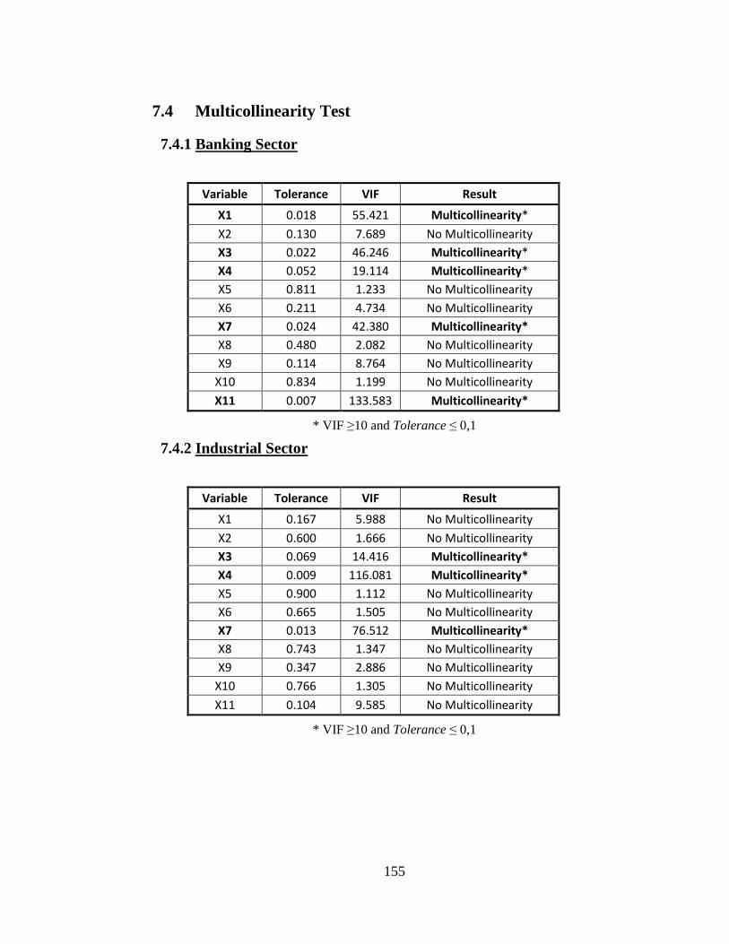
155
7.4 Multicollinearity Test
7.4.1 Banking Sector
Variable Tolerance VIF Result
X1 0.018 55.421 Multicollinearity*
X2 0.130 7.689 No Multicollinearity
X3 0.022 46.246 Multicollinearity*
X4 0.052 19.114 Multicollinearity*
X5 0.811 1.233 No Multicollinearity
X6 0.211 4.734 No Multicollinearity
X7 0.024 42.380 Multicollinearity*
X8 0.480 2.082 No Multicollinearity
X9 0.114 8.764 No Multicollinearity
X10 0.834 1.199 No Multicollinearity
X11 0.007 133.583 Multicollinearity*
* VIF ≥10 and Tolerance ≤ 0,1 7.4.2 Industrial Sector
Variable Tolerance VIF Result
X1 0.167 5.988 No Multicollinearity
X2 0.600 1.666 No Multicollinearity
X3 0.069 14.416 Multicollinearity*
X4 0.009 116.081 Multicollinearity*
X5 0.900 1.112 No Multicollinearity
X6 0.665 1.505 No Multicollinearity
X7 0.013 76.512 Multicollinearity*
X8 0.743 1.347 No Multicollinearity
X9 0.347 2.886 No Multicollinearity
X10 0.766 1.305 No Multicollinearity
X11 0.104 9.585 No Multicollinearity
* VIF ≥10 and Tolerance ≤ 0,1
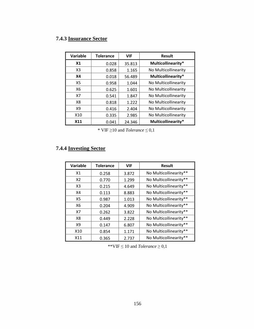
156
7.4.3 Insurance Sector
Variable Tolerance VIF Result
X1 0.028 35.813 Multicollinearity*
X3 0.858 1.165 No Multicollinearity
X4 0.018 56.489 Multicollinearity*
X5 0.958 1.044 No Multicollinearity
X6 0.625 1.601 No Multicollinearity
X7 0.541 1.847 No Multicollinearity
X8 0.818 1.222 No Multicollinearity
X9 0.416 2.404 No Multicollinearity
X10 0.335 2.985 No Multicollinearity
X11 0.041 24.346 Multicollinearity*
* VIF ≥10 and Tolerance ≤ 0,1
7.4.4 Investing Sector
Variable Tolerance VIF Result
X1 0.258 3.872 No Multicollinearity**
X2 0.770 1.299 No Multicollinearity**
X3 0.215 4.649 No Multicollinearity**
X4 0.113 8.883 No Multicollinearity**
X5 0.987 1.013 No Multicollinearity**
X6 0.204 4.909 No Multicollinearity**
X7 0.262 3.822 No Multicollinearity**
X8 0.449 2.228 No Multicollinearity**
X9 0.147 6.807 No Multicollinearity**
X10 0.854 1.171 No Multicollinearity**
X11 0.365 2.737 No Multicollinearity**
**VIF ≤ 10 and Tolerance ≥ 0,1
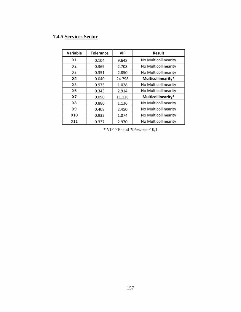
157
7.4.5 Services Sector
Variable Tolerance VIF Result
X1 0.104 9.648 No Multicollinearity
X2 0.369 2.708 No Multicollinearity
X3 0.351 2.850 No Multicollinearity
X4 0.040 24.798 Multicollinearity*
X5 0.973 1.028 No Multicollinearity
X6 0.343 2.914 No Multicollinearity
X7 0.090 11.126 Multicollinearity*
X8 0.880 1.136 No Multicollinearity
X9 0.408 2.450 No Multicollinearity
X10 0.932 1.074 No Multicollinearity
X11 0.337 2.970 No Multicollinearity
* VIF ≥10 and Tolerance ≤ 0,1