The Islamic University of Gaza Faculty of Engineering...
38
1 Adapted from lectures of Prof. Rifat Rustom S Associate Prof. Mazen Abualtayef Civil Engineering Department, The Islamic University of Gaza The Islamic University of Gaza Faculty of Engineering Civil Engineering Department Numerical Analysis ECIV 3306 Chapter 15 Optimization
Transcript of The Islamic University of Gaza Faculty of Engineering...
1
Adapted from lectures
of Prof. Rifat Rustom
S
Associate Prof. Mazen Abualtayef
Civil Engineering Department, The Islamic University of Gaza
The Islamic University of Gaza
Faculty of Engineering
Civil Engineering Department
Numerical Analysis
ECIV 3306
Chapter 15
Optimization
2
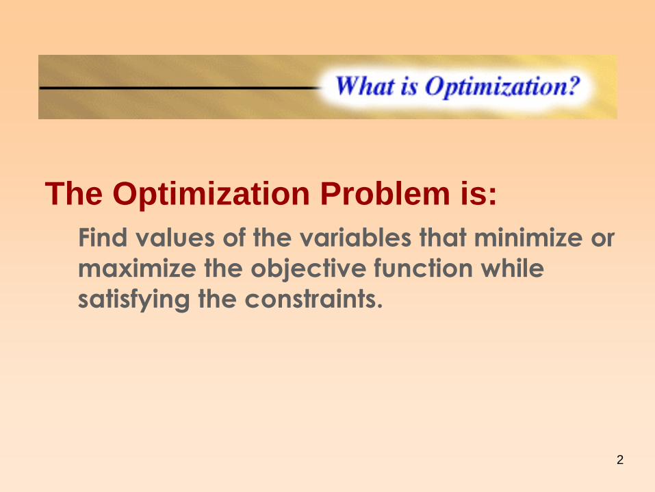
What is Optimization
The Optimization Problem is:
Find values of the variables that minimize or
maximize the objective function while
satisfying the constraints.

3
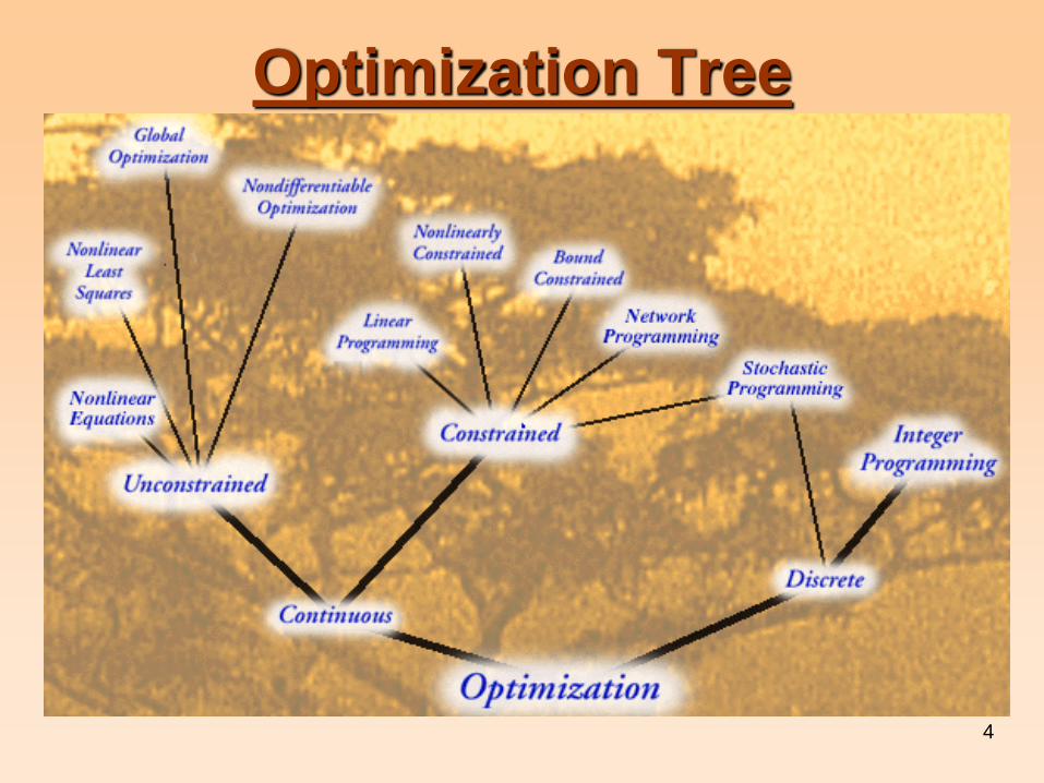
Components of Optimization
Problem
Optimization
problems are made up
of three basic
ingredients:
An objective function which
we want to minimize or
maximize
A set of unknowns or
variables which affect the
value of the objective function
A set of constraints that
allow the unknowns to take on
certain values but exclude
others
4
Optimization Tree
5
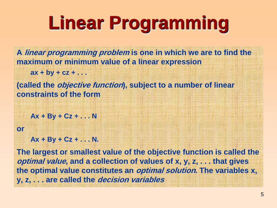
Linear Programming
A linear programming problem is one in which we are to find the
maximum or minimum value of a linear expression
ax + by + cz + . . .
(called the objective function), subject to a number of linear
constraints of the form
Ax + By + Cz + . . . N
or
Ax + By + Cz + . . . N.
The largest or smallest value of the objective function is called the
optimal value, and a collection of values of x, y, z, . . . that gives
the optimal value constitutes an optimal solution. The variables x,
y, z, . . . are called the decision variables

LP Properties and Assumptions PROPERTIES OF LINEAR PROGRAMS
1. One objective function
2. One or more constraints
3. Alternative courses of action
4. Objective function and constraints are linear
ASSUMPTIONS OF LP
1. Certainty
2. Proportionality
3. Additivity
4. Divisibility
5. Nonnegative variables
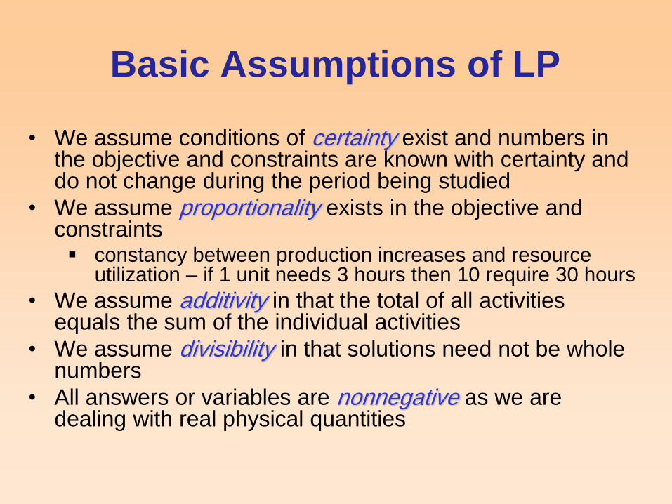
Basic Assumptions of LP
• We assume conditions of certainty exist and numbers in the objective and constraints are known with certainty and do not change during the period being studied
• We assume proportionality exists in the objective and constraints constancy between production increases and resource
utilization – if 1 unit needs 3 hours then 10 require 30 hours
• We assume additivity in that the total of all activities equals the sum of the individual activities
• We assume divisibility in that solutions need not be whole numbers
• All answers or variables are nonnegative as we are dealing with real physical quantities
8
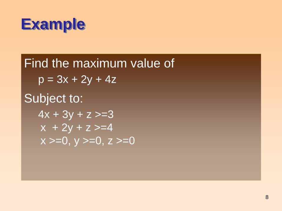
Example
Find the maximum value of
p = 3x + 2y + 4z
Subject to:
4x + 3y + z >=3
x + 2y + z >=4
x >=0, y >=0, z >=0
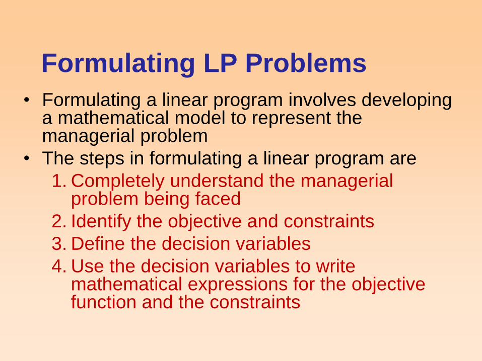
Formulating LP Problems
• Formulating a linear program involves developing a mathematical model to represent the managerial problem
• The steps in formulating a linear program are
1. Completely understand the managerial problem being faced
2. Identify the objective and constraints
3. Define the decision variables
4. Use the decision variables to write mathematical expressions for the objective function and the constraints
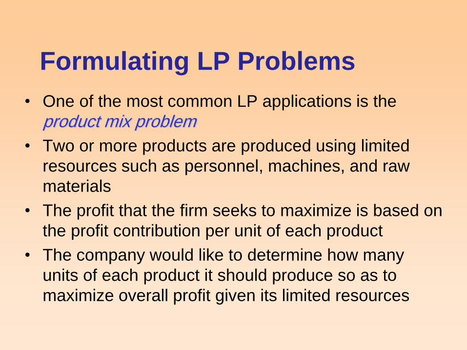
Formulating LP Problems
• One of the most common LP applications is the
product mix problem
• Two or more products are produced using limited
resources such as personnel, machines, and raw
materials
• The profit that the firm seeks to maximize is based on
the profit contribution per unit of each product
• The company would like to determine how many
units of each product it should produce so as to
maximize overall profit given its limited resources
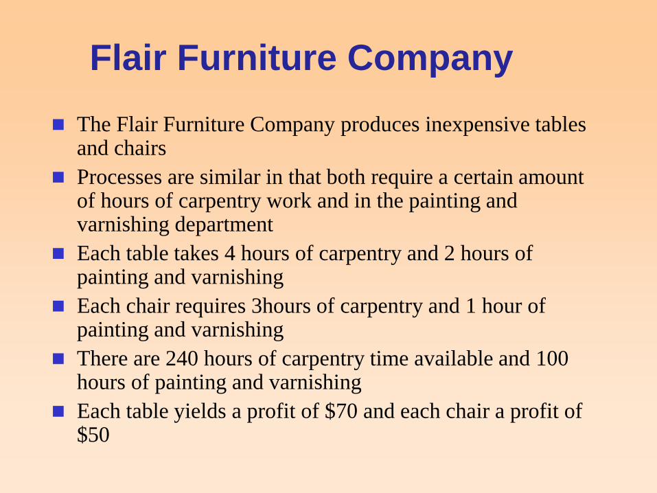
Flair Furniture Company
The Flair Furniture Company produces inexpensive tables and chairs
Processes are similar in that both require a certain amount of hours of carpentry work and in the painting and varnishing department
Each table takes 4 hours of carpentry and 2 hours of painting and varnishing
Each chair requires 3hours of carpentry and 1 hour of painting and varnishing
There are 240 hours of carpentry time available and 100 hours of painting and varnishing
Each table yields a profit of $70 and each chair a profit of $50

Flair Furniture Company
The company wants to determine the best combination of tables and chairs to produce to reach the maximum profit
HOURS REQUIRED TO PRODUCE 1 UNIT
DEPARTMENT (T)
TABLES (C)
CHAIRS AVAILABLE HOURS THIS WEEK
Carpentry 4 3 240
Painting and varnishing 2 1 100
Profit per unit $70 $50
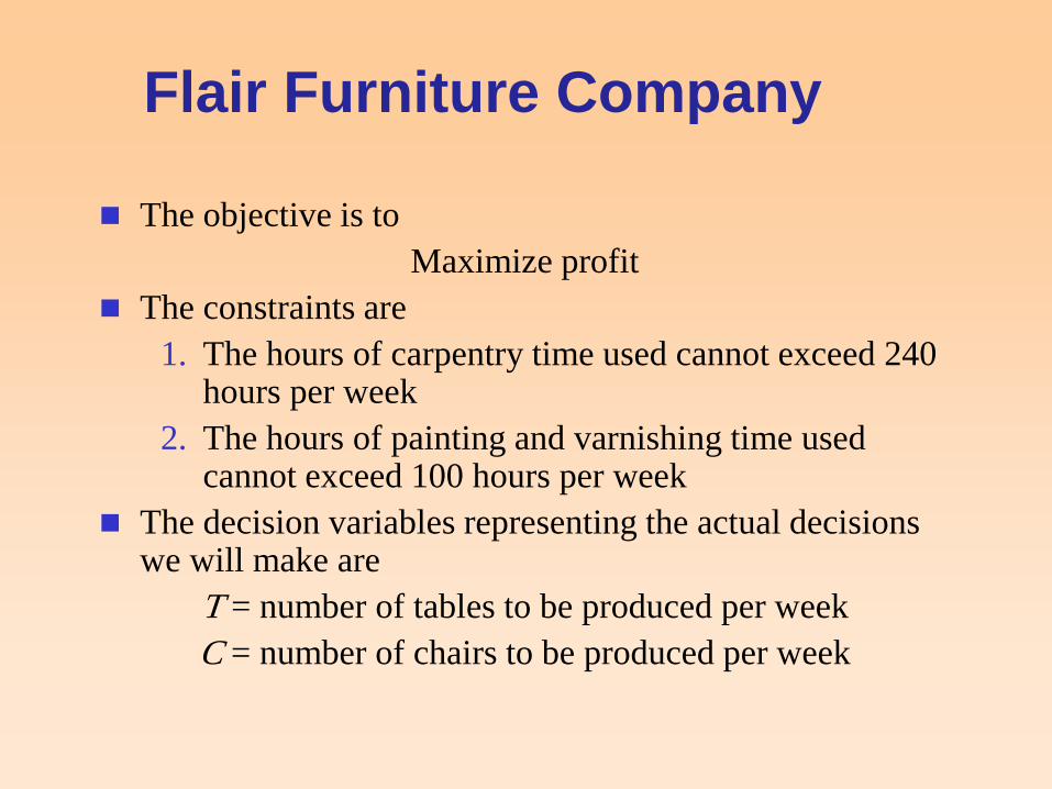
Flair Furniture Company
The objective is to
Maximize profit
The constraints are
1. The hours of carpentry time used cannot exceed 240 hours per week
2. The hours of painting and varnishing time used cannot exceed 100 hours per week
The decision variables representing the actual decisions we will make are
T = number of tables to be produced per week
C = number of chairs to be produced per week
Flair Furniture Company
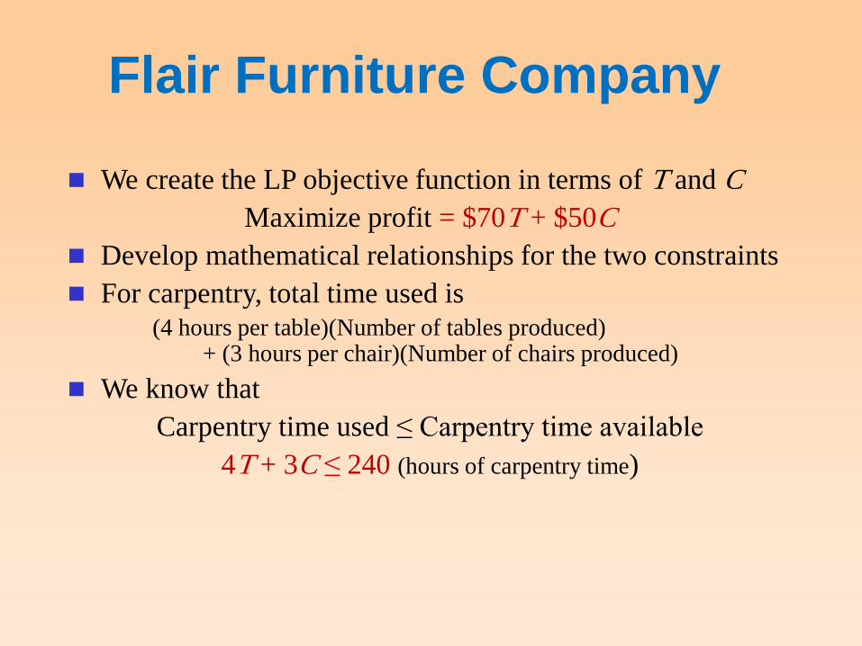
We create the LP objective function in terms of T and C
Maximize profit = $70T + $50C
Develop mathematical relationships for the two constraints
For carpentry, total time used is
(4 hours per table)(Number of tables produced) + (3 hours per chair)(Number of chairs produced)
We know that
Carpentry time used ≤ Carpentry time available
4T + 3C ≤ 240 (hours of carpentry time)
Flair Furniture Company
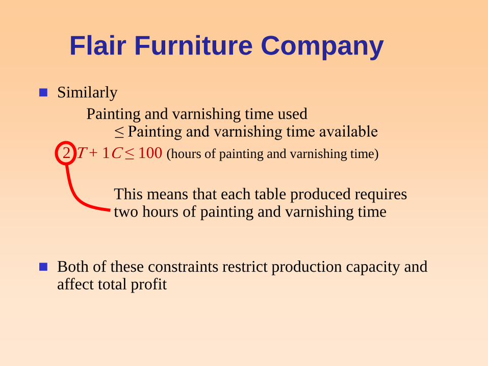
Similarly
Painting and varnishing time used ≤ Painting and varnishing time available
2 T + 1C ≤ 100 (hours of painting and varnishing time)
This means that each table produced requires two hours of painting and varnishing time
Both of these constraints restrict production capacity and affect total profit

Flair Furniture Company
The values for T and C must be nonnegative
T ≥ 0 (number of tables produced is greater than or equal to 0)
C ≥ 0 (number of chairs produced is greater than or equal to 0)
The complete problem stated mathematically
Maximize profit = $70T + $50C
subject to
4T + 3C ≤ 240 (carpentry constraint)
2T + 1C ≤ 100 (painting and varnishing constraint)
T, C ≥ 0 (nonnegativity constraint)

Max 70T + 50C
Subject to
4T + 3C <=240
2T + 1C <=100
T >= 0
C >= 0
Global optimal solution found.
Objective value: 4100.000
Infeasibilities: 0.000000
Total solver iterations: 2
Model Class: LP
Total variables: 2
Nonlinear variables: 0
Integer variables: 0
Total constraints: 5
Nonlinear constraints: 0
Total nonzeros: 8
Nonlinear nonzeros: 0
Variable Value Reduced Cost
T 30.00000 0.000000
C 40.00000 0.000000
Row Slack or Surplus Dual Price
1 4100.000 1.000000
2 0.000000 15.00000
3 0.000000 5.000000
4 30.00000 0.000000
5 40.00000 0.000000
18
19
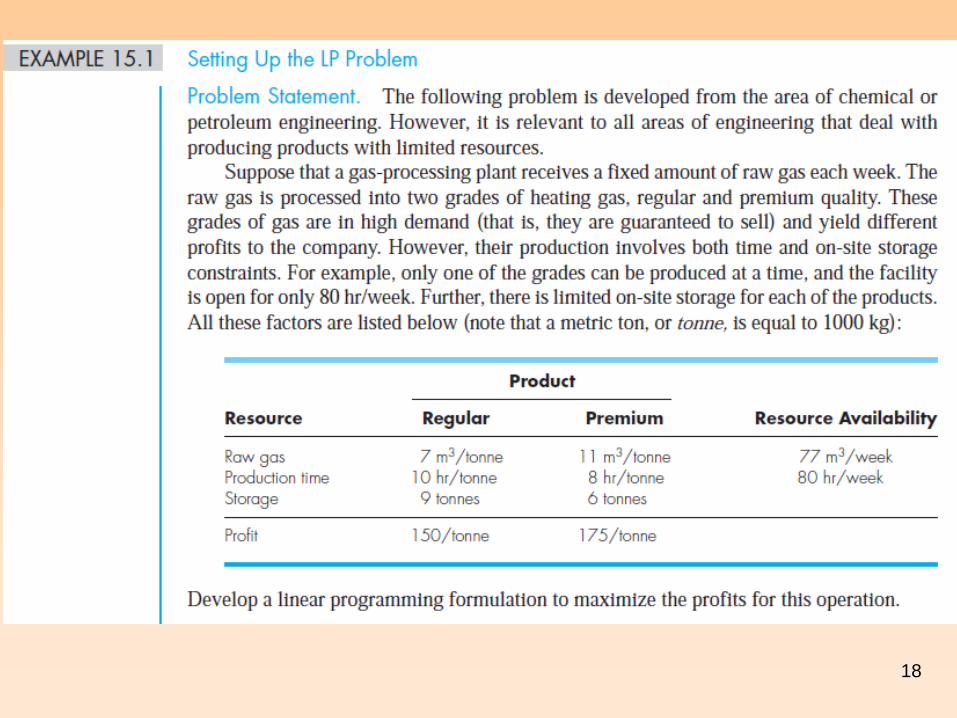
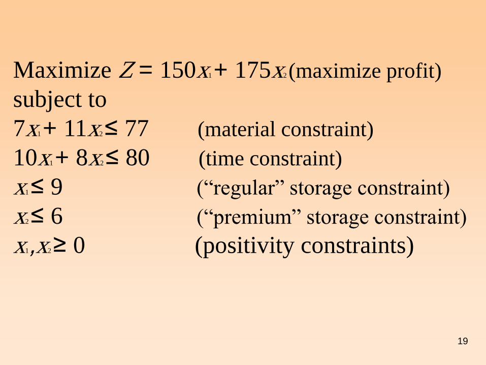
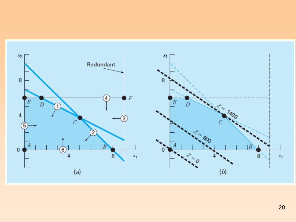
Maximize Z = 150x1 + 175x2 (maximize profit)
subject to
7x1 + 11x2 ≤ 77 (material constraint)
10x1 + 8x2 ≤ 80 (time constraint)
x1 ≤ 9 (“regular” storage constraint)
x2 ≤ 6 (“premium” storage constraint)
x1,x2 ≥ 0 (positivity constraints)
20
21
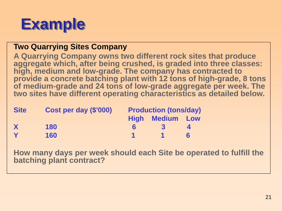
Example
Two Quarrying Sites Company
A Quarrying Company owns two different rock sites that produce aggregate which, after being crushed, is graded into three classes: high, medium and low-grade. The company has contracted to provide a concrete batching plant with 12 tons of high-grade, 8 tons of medium-grade and 24 tons of low-grade aggregate per week. The two sites have different operating characteristics as detailed below.
Site Cost per day ($'000) Production (tons/day)
High Medium Low
X 180 6 3 4
Y 160 1 1 6
How many days per week should each Site be operated to fulfill the batching plant contract?
22
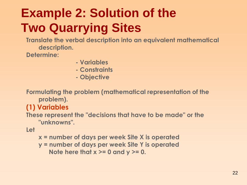
Example 2: Solution of the
Two Quarrying Sites
Translate the verbal description into an equivalent mathematical
description.
Determine:
- Variables
- Constraints
- Objective
Formulating the problem (mathematical representation of the
problem).
(1) Variables
These represent the "decisions that have to be made" or the
"unknowns".
Let
x = number of days per week Site X is operated
y = number of days per week Site Y is operated
Note here that x >= 0 and y >= 0.
23
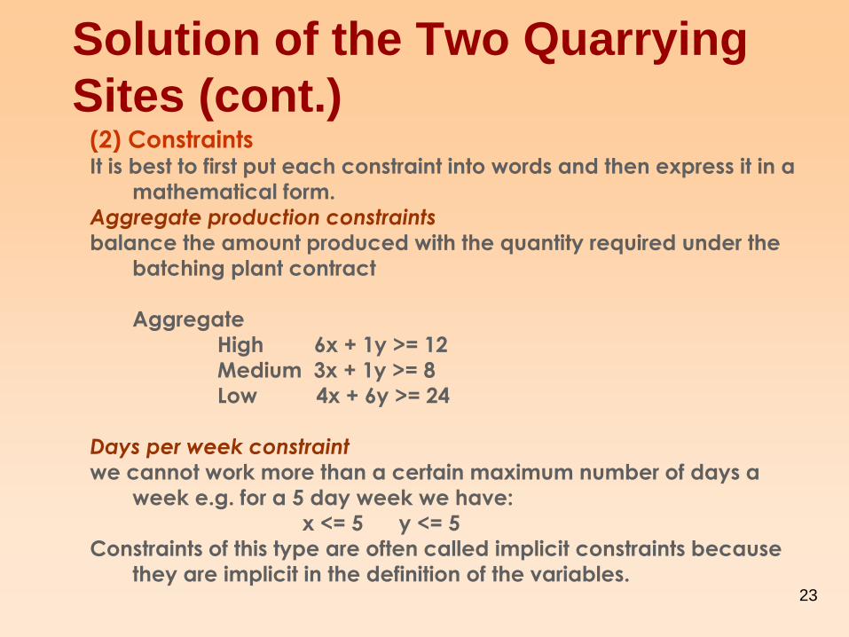
Solution of the Two Quarrying
Sites (cont.) (2) Constraints
It is best to first put each constraint into words and then express it in a
mathematical form.
Aggregate production constraints
balance the amount produced with the quantity required under the
batching plant contract
Aggregate
High 6x + 1y >= 12
Medium 3x + 1y >= 8
Low 4x + 6y >= 24
Days per week constraint
we cannot work more than a certain maximum number of days a
week e.g. for a 5 day week we have:
x <= 5 y <= 5
Constraints of this type are often called implicit constraints because
they are implicit in the definition of the variables.

24
Solution of the Two Quarrying
Sites (cont.) (3) Objective
Again in words our objective is (presumably) to minimize cost which
is given by 180x + 160y
Hence we have the complete mathematical representation of the
problem as:
minimize 180x + 160y Subject to
6x + y >= 12
3x + y >= 8
4x + 6y >= 24 x <= 5
y <= 5
x,y >= 0

25
Problem Statement:
Three wells in Gaza are used to pump water for
domestic use. The maximum discharge of the wells
as well as the properties of water pumped are shown
in the table below. The water is required to be treated
using chlorine before pumped into the system
Determine the minimum cost of chlorine treatment per
cubic meter per day for the three wells given the cost in
$/m3 for the three wells. Total discharge should be equal
to 5000 m3/day.
Case 1: Optimization of Well Treatment

26
Cl Qmax Cl treatment max working
mg/l m3/hr. $/m3 hours
Well No. 1 200 100 0.05 20
Well No. 2 500 150 0.12 18
Well No. 3 300 200 0.08 15
PROPERTIES OF PUMPED WATER
27
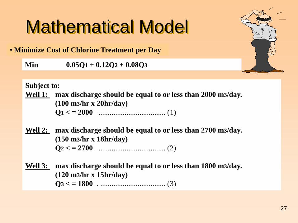
Mathematical Model • Minimize Cost of Chlorine Treatment per Day
Min 0.05Q1 + 0.12Q2 + 0.08Q3
Subject to:
Well 1: max discharge should be equal to or less than 2000 m3/day.
(100 m3/hr x 20hr/day)
Q1 < = 2000 .................................... (1)
Well 2: max discharge should be equal to or less than 2700 m3/day.
(150 m3/hr x 18hr/day)
Q2 < = 2700 .................................... (2)
Well 3: max discharge should be equal to or less than 1800 m3/day.
(120 m3/hr x 15hr/day)
Q3 < = 1800 . ................................... (3)
28
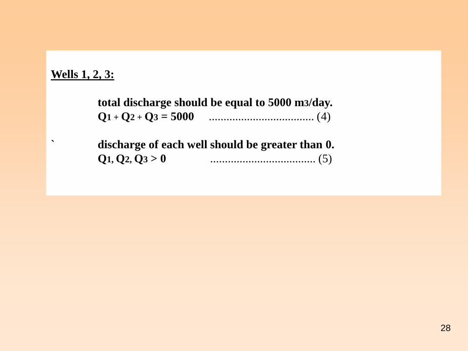
Wells 1, 2, 3:
total discharge should be equal to 5000 m3/day.
Q1 + Q2 + Q3 = 5000 .................................... (4)
` discharge of each well should be greater than 0.
Q1, Q2, Q3 > 0 .................................... (5)
29
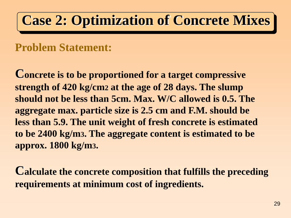
Problem Statement:
Concrete is to be proportioned for a target compressive
strength of 420 kg/cm2 at the age of 28 days. The slump
should not be less than 5cm. Max. W/C allowed is 0.5. The
aggregate max. particle size is 2.5 cm and F.M. should be
less than 5.9. The unit weight of fresh concrete is estimated
to be 2400 kg/m3. The aggregate content is estimated to be
approx. 1800 kg/m3.
Calculate the concrete composition that fulfills the preceding
requirements at minimum cost of ingredients.
Case 2: Optimization of Concrete Mixes
30
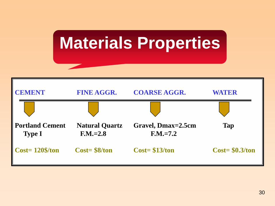
Materials Properties
CEMENT FINE AGGR. COARSE AGGR. WATER
Portland Cement Natural Quartz Gravel, Dmax=2.5cm Tap
Type I F.M.=2.8 F.M.=7.2
Cost= 120$/ton Cost= $8/ton Cost= $13/ton Cost= $0.3/ton

31
Mathematical Model • Minimize Cost of Concrete Composition per m3
Objective Function: C = 0.12C + 0.008S + 0.013G + 0.0003W
• Constraints
Subject to:
Strength: f’c= 230(C/W - 0.5) should be greater than 420 kg/cm2
230(C/W - 0.5) > = 420 .................................... (1)
c - 2.346w > = 0
Water- Cement ratio:
W/C < = 0.5 .................................... (2)
Consistency: W= 0.072C + 20.43(11-F.M.) for 5cm slump,
Grading: where F.M.= (2.8S + 7.2G)/1800,
F.M.< = 5.9
Experimental
relationship

32
(2.80S + 7.20G)/1800 < = 5.9 . ................................... (3)
Unit Weight: Total weights of all ingredients per m3 should be equal to
the Unit Weight of fresh concrete.
C + W + S + G = 2400 . ................................... (4)
Non Negativity:
C, W, S , G >= 0 . ................................... (5)

33
Case Studies (Work in Class)
Case 1 A developer has the alternative of building two, three, and four- bedroom houses. He wishes
to establish the number of each, if any, that will maximize his profit, subject to the following
constraints:
1-The total budget for the project cannot exceed $ 9,000,000
2-The total number of units must be at least 350 for the venture to be economically feasible.
3-The maximum percentages of each type, based on an analysis of the market, are :
2- bedroom units, 20% of total
3-bedroom units, 60% of total
4-bedroom units, 40% of total
4- Building costs including land, architectural and engineer. fees, landscaping, and so on are:
2- bedroom unit, $20,000
3-bedroom unit, $25,000
4-bedroom unit, $30,000
5- Net profits after interest, taxes, and so on, are
2- bedroom unit, $ 2,000
3-bedroom unit, $3,000
4-bedroom unit, $4,000
34
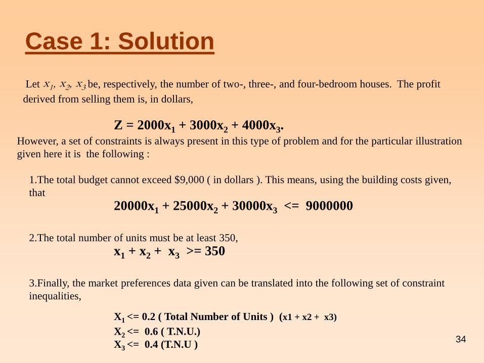
Case 1: Solution
Let x1, x2, x3 be, respectively, the number of two-, three-, and four-bedroom houses. The profit
derived from selling them is, in dollars,
Z = 2000x1 + 3000x2 + 4000x3. However, a set of constraints is always present in this type of problem and for the particular illustration
given here it is the following :
1.The total budget cannot exceed $9,000 ( in dollars ). This means, using the building costs given,
that
20000x1 + 25000x2 + 30000x3 <= 9000000 2.The total number of units must be at least 350,
x1 + x2 + x3 >= 350 3.Finally, the market preferences data given can be translated into the following set of constraint
inequalities,
X1 <= 0.2 ( Total Number of Units ) (x1 + x2 + x3) X2 <= 0.6 ( T.N.U.)
X3 <= 0.4 (T.N.U )
35
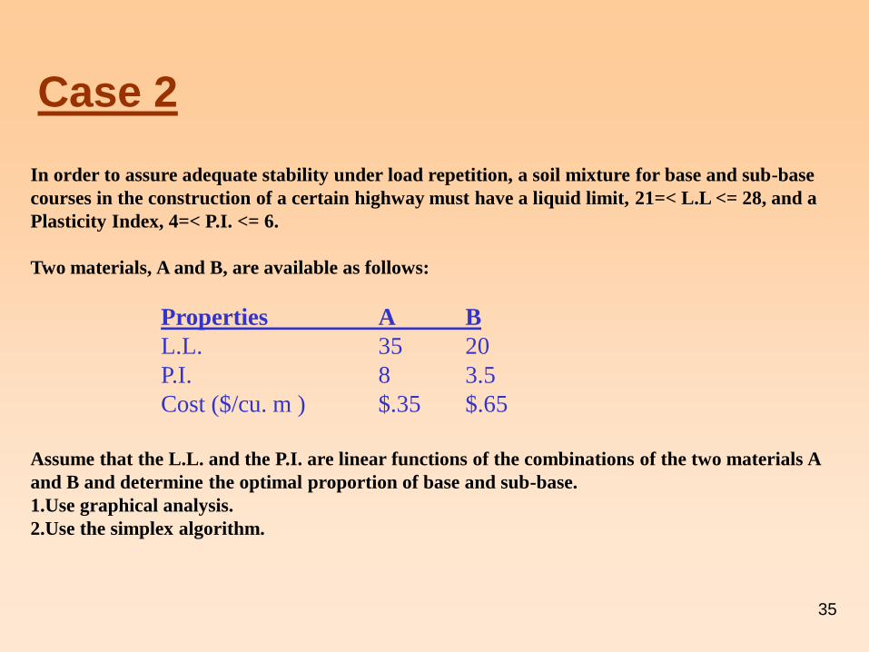
Case 2
In order to assure adequate stability under load repetition, a soil mixture for base and sub-base
courses in the construction of a certain highway must have a liquid limit, 21=< L.L <= 28, and a
Plasticity Index, 4=< P.I. <= 6.
Two materials, A and B, are available as follows:
Properties A B
L.L. 35 20
P.I. 8 3.5
Cost ($/cu. m ) $.35 $.65
Assume that the L.L. and the P.I. are linear functions of the combinations of the two materials A
and B and determine the optimal proportion of base and sub-base.
1.Use graphical analysis.
2.Use the simplex algorithm.
36
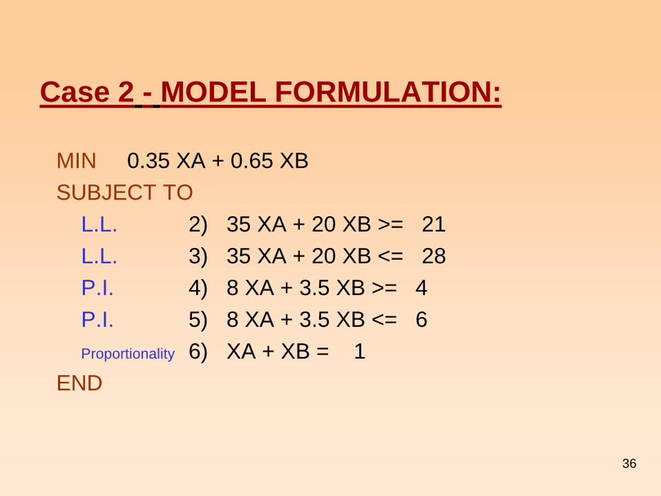
Case 2 - MODEL FORMULATION:
MIN 0.35 XA + 0.65 XB
SUBJECT TO
L.L. 2) 35 XA + 20 XB >= 21
L.L. 3) 35 XA + 20 XB <= 28
P.I. 4) 8 XA + 3.5 XB >= 4
P.I. 5) 8 XA + 3.5 XB <= 6
Proportionality 6) XA + XB = 1
END
37
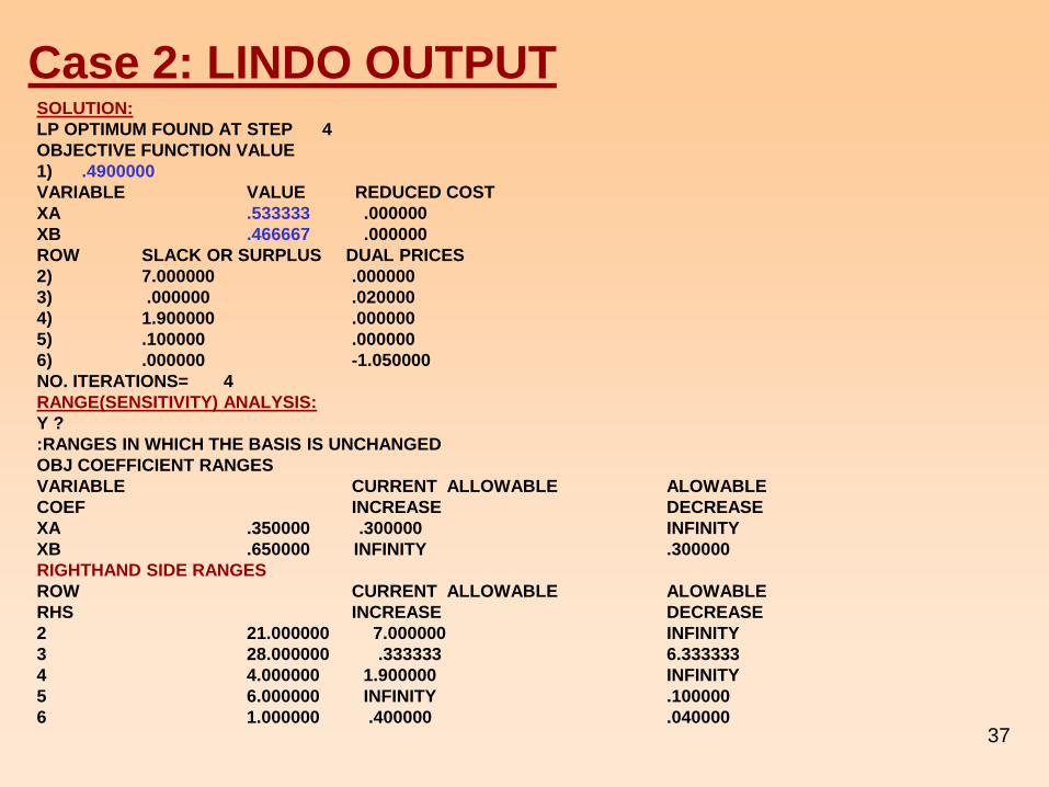
Case 2: LINDO OUTPUT SOLUTION:
LP OPTIMUM FOUND AT STEP 4
OBJECTIVE FUNCTION VALUE
1) .4900000
VARIABLE VALUE REDUCED COST
XA .533333 .000000
XB .466667 .000000
ROW SLACK OR SURPLUS DUAL PRICES
2) 7.000000 .000000
3) .000000 .020000
4) 1.900000 .000000
5) .100000 .000000
6) .000000 -1.050000
NO. ITERATIONS= 4
RANGE(SENSITIVITY) ANALYSIS:
Y ?
:RANGES IN WHICH THE BASIS IS UNCHANGED
OBJ COEFFICIENT RANGES
VARIABLE CURRENT ALLOWABLE ALOWABLE
COEF INCREASE DECREASE
XA .350000 .300000 INFINITY
XB .650000 INFINITY .300000
RIGHTHAND SIDE RANGES
ROW CURRENT ALLOWABLE ALOWABLE
RHS INCREASE DECREASE
2 21.000000 7.000000 INFINITY
3 28.000000 .333333 6.333333
4 4.000000 1.900000 INFINITY
5 6.000000 INFINITY .100000
6 1.000000 .400000 .040000

38
Case Studies (Work in Class)
Case 3 A Mat Foundation (500 m3) need to be cast. Thee concrete batching
plants could be used to deliver concrete to the site. The relevant data
associated with these plants are given below. Formulate the LP
problem to minimize the cost of casting the Mat Foundation given that
the casting time allowed is 6 hours.
No. of Available Transit Mixers
(Size)
Daily
Production
Transport
Time
Cost Concrete
Batch
Plant
6 m3 8 m3 10 m3 (m3/day) min. ($/m3 )
5 3 2 300 30 120 A
2 3 5 350 45 110 B
5 2 3 400 50 130 C