The Irrevocable Multi-Armed Bandit Problem

Vivek F. Farias ∗ Ritesh Madan †

22 June 2008Revised: 16 June 2009

Abstract

This paper considers the multi-armed bandit problem with multiple simultaneous arm pullsand the additional restriction that we do not allow recourse to arms that were pulled at somepoint in the past but then discarded. This additional restriction is highly desirable from anoperational perspective and we refer to this problem as the ‘Irrevocable Multi-Armed Bandit’problem. We observe that natural modifications to well known heuristics for multi-armed banditproblems that satisfy this irrevocability constraint have unsatisfactory performance, and thusmotivated introduce a new heuristic: the ‘packing’ heuristic. We establish through numericalexperiments that the packing heuristic offers excellent performance, even relative to heuristicsthat are not constrained to be irrevocable. We also provide a theoretical analysis that studies the‘price’ of irrevocability i.e. the performance loss incurred in imposing the constraint we proposeon the multi-armed bandit model. We show that this performance loss is uniformly boundedfor a general class of multi-armed bandit problems, and also indicate its dependence on variousproblem parameters. Finally, we obtain a computationally fast algorithm to implement thepacking heuristic; the algorithm renders the packing heuristic computationally cheaper thanmethods that rely on the computation of Gittins indices.

1. Introduction

Consider the operations of a ‘fast-fashion’ retailer such as Zara or H&M. Such retailers have devel-oped and invested in merchandise procurement strategies that permit lead times for new fashionsas short as two weeks. As a consequence of this flexibility, such retailers are able to adjust theassortment of products offered on sale at their stores to quickly adapt to popular fashion trends. Inparticular, such retailers use weekly sales data to refine their estimates of an item’s popularity, andbased on such revised estimates weed out unpopular items, or else re-stock demonstrably popularones on a week-by-week basis. In view of the great deal of a-priori uncertainty in the popularity ofa new fashion and the speed at which fashion trends evolve, the fast-fashion operations model ishighly desirable and emerging as the de-facto operations model for large fashion retailers.

Among other things, the fast-fashion model relies crucially on an effective technology to learnfrom purchase data, and adjust product assortments based on such data. Such a technology muststrike a balance between ‘exploring’ potentially successful products and ‘exploiting’ products that∗Sloan School of Management and Operations Research Center, Massachusetts Institute of Technology, email

:vivekf@mit.edu†Qualcomm-Flarion Technologies, email :rkmadan@stanfordalumni.org

1

are demonstrably popular. A convenient mathematical model within which to design algorithmscapable of accomplishing such a task is that of the multi-armed bandit. While we defer a precisemathematical discussion to a later section, a multi-armed bandit consists of multiple (say n) ‘arms’,each corresponding to a Markov Decision Process. As a special case, one may think of each arm as anindependent Bernoulli random variable with an uncertain bias specified via some prior distribution.At each point in time, one may ‘pull’ up to a certain number of arms (say k < n) simultaneously.For each arm pulled, we modify our estimate of its bias based on its realization and earn a rewardproportional to its realization. We neither learn about, nor earn rewards from arms that are notpulled. The multi-armed bandit problem requires finding a policy that adaptively selects k arms topull at every point in time with an objective of maximizing total expected reward earned over somefinite time horizon or alternatively, discounted rewards earned over an infinite horizon or perhaps,even long term average rewards.

The multi-armed bandit model while general and immensely useful, fails to capture an importantrestriction one faces in several applications. In particular, in a number of applications, the act of‘pulling’ an arm that has been pulled in the past but discarded in favor of another arm is undesirableor unacceptable. Ignoring references to the extant literature for now, examples of such applicationsinclude:

1. Fast Fashion: The fixed costs associated with the introduction of a new product make frequentchanges in the assortment of products offered undesirable. More importantly, fast fashionretailers rely heavily on discouraging their customers from delaying/ strategizing on the timingof their purchase decisions. They accomplish this by adhering to strict restocking policies;reintroduction of an old product is undesirable from this viewpoint.

2. Call-Center Hiring: Given the rich variety of tasks call-center workers might face, recentresearch has raised the possibility of ‘data-driven’ hiring/ staff allocation decisions at call-centers. In this setting, the act of discarding an arm is equivalent to a firing or reassignmentdecision; it is clear that such decisions are difficult to reverse.

3. Clinical Trials: A classical application of the bandit model, the act of discarding an arm inthis setting is equivalent to the discontinuation of trials on a particular treatment. The ethicalobjections to administering treatments that may be viewed as inferior play a critical role inthe design of such trials and it is reasonable to expect that re-starting trials on a procedureafter a hiatus might well raise ethical concerns.

This paper considers the multi-armed bandit problem with an additional restriction: we requirethat decisions to remove an arm from the set of arms currently being pulled be ‘irrevocable’. Thatis, we do not allow recourse to arms that were pulled at some point in the past but then discarded.We refer to this problem as the Irrevocable Multi-Armed Bandit Problem. We introduce a novelheuristic we call the ‘packing’ heuristic for this problem. The packing heuristic establishes a staticranking of bandit arms based on a measure of their potential value relative to the time requiredto realize that value, and pulls arms in the order prescribed by this ranking. For an arm currentlybeing pulled, the heuristic may either choose to continue pulling that arm in the next time stepor else discard the arm in favor of the next highest ranked arm not currently being pulled. Oncediscarded, an arm will never be chosen again hence satisfying the irrevocability constraint. Wedemonstrate via computational experiments that the use of the packing heuristic incurs a small

2

performance loss relative to an optimal bandit policy without the irrevocability constraint. Ingreater detail, the present work makes the following contributions:

• We introduce the irrevocable multi-armed bandit problem and develop a heuristic for itssolution motivated by recent advances in the study of stochastic packing. We present acomputational study which demonstrates that the performance of the packing heuristic com-pares favorably with a computable upper bound on the performance of any (potentially non-irreovocable) multi-armed bandit policy. We compare the performance of the packing heuris-tic with that of a heuristic originally proposed by Whittle (which is not irrevocable) and anatural irrevocable version of Whittle’s heuristic. We find that the packing heuristic offerssubstantial performance gains over the irrevocable version of Whittle’s heuristic we consider.Further we observe that the number of ‘revocations’ of an arm under Whittle’s heuristic issubstantial while offering only a modest improvement over the packing heuristic.

• We present a theoretical analysis to bound the performance loss incurred relative to an optimalpolicy with no restrictions on irrevocability. We characterize a general class of bandits forwhich this ‘price of irrevocability’ is uniformly bounded. We show that this class of banditsadmits the ‘learning’ applications we have alluded to thus far. For bandits within this class,we show that the packing heuristic earns expected rewards that are always within a factor of1/8 of an optimal policy for the classical multi-armed bandit. We present stronger boundsby allowing for a dependence on problem parameters such as the number of bandits and thedegree of parallelism (i.e. the ratio k/n). For instance, we show that in a natural scalingregime first proposed by Whittle, the above bound can be improved by a factor of 2. Thesebounds imply, to the best of our knowledge, the first performance bounds for an importantgeneral class of bandit problems with multiple simultaneous pulls over a finite time horizon.We introduce a mode of analysis distinct from the ‘mean-field’ techniques used for banditproblems with the long run average reward criterion 1; these latter techniques do not applyto finite horizon problems.

An additional outcome of this analysis is that we establish a precise connection betweenstochastic packing problems and the multi-armed bandit problem; we anticipate that thisconnection can serve as a useful tool for the further design and analysis of algorithms forbandit problems.

• In the interest of practical applicability, we develop a fast, essentially combinatorial imple-mentation of the packing heuristic. Assuming that an individual arm has O(Σ) states, andgiven a time horizon of T steps, an optimal solution to the multi-armed bandit problemunder consideration requires O(ΣnTn) computations. The main computational step in thepacking heuristic calls for the one time solution of a linear program with O(nΣT ) variables,whose solution via a generic LP solver requires O(n3Σ3T 3) computations. We develop analgorithm that solves this linear program in O(nΣ2T log T ) steps by solving a sequence ofdynamic programs for each bandit arm. The technique we develop here is potentially of inde-pendent interest for the solution of ‘weakly coupled’ optimal control problems with couplingconstraints that must be met in expectation. Employing this solution technique, our heuristic

1we discuss why the average reward criterion is uninteresting for Bayesian learning problems in Section 1.1

3

requires a total of O(nΣ2 log T ) computations per time step amortized over the time horizon.In contrast, Whittle’s heuristic (or the irrevocable version of that heuristic we consider) re-quires O(nΣ2T log T ) computations per time step. Given the substantial amount of researchthat has been dedicated to simply calculating Gittins indices (in the context of Whittle’sheuristic) rapidly, this is a notable contribution. More importantly, we establish that thepacking heuristic is computationally attractive.

1.1. Relevant Literature

The multi-armed bandit problem has a rich history, and a number of excellent references (such asGittins (1989)) provide a thorough treatment of the subject. Our consideration of the ‘irrevocable’multi-armed bandit problem stems from a number of applications of the bandit framework alluded toearlier. Caro and Gallien (2007) have considered using the multi-armed bandit for the assortmentdesign problem faced by fast fashion retailers. Pich and Van der Heyden (2002) emphasize theimportance of not allowing for ‘repeat’ products in an assortment in that setting. Arlotto et al.(2009) consider the application of the multi-armed bandit model in the context of ascertainingthe suitability of individuals for a given task at a call-center. The methodology suggested by theauthors respects the irrevocability constraint studied here and is similar to the irrevocable versionof Whittle’s heuristic we examine. This constraint is quite natural to their setting as firing decisionsare difficult to reverse. Finally, there is a very large and varied literature on the design of clinicaltrials and we make no attempt to review that here. ‘Ethical’ experimentation policies are anoverriding theme of much of the work in this area; see Anscombe (1963) for an early treatment onthe subject and Armitage et al. (2002) for a more recent overview.

There has been a great deal of work on heuristics for the multi-armed bandit problem. In thecase where k = 1, that is, allowing for a single arm to be pulled in a given time step, Gittinsand Jones (1974) developed an elegant index based policy that was shown to be optimal for theproblem of maximizing discounted rewards over an infinite horizon. Their index policy is known tobe suboptimal if one is allowed to pull more than a single arm in a given time step. Whittle (1988)developed a simple index based heuristic for a more general bandit problem (the ‘restless’ banditproblem) allowing for multiple arms to be pulled in a given time step. While his original paperwas concerned with maximizing long-term average rewards, his heuristic is easily adapted to otherobjectives such as discounted infinite horizon rewards or expected rewards over a finite horizon (seefor instance Bertsimas and Nino-Mora (2000); Caro and Gallien (2007)). It is important to note,however, that much of the extant performance analysis for bandit problems (beyond the initialwork of Gittins and Jones (1974)) in general, and Whittle’s heuristic in particular, focuses onbandits with a single recurrent class and the average cost/reward criterion. In that setting Weberand Weiss (1990) presented a set of technical conditions that guarantee that Whittle’s heuristic isasymptotically optimal (in a regime where n and k go to infinity keeping n/k constant) for thegeneral restless bandit problem and further, that Whittle’s heuristic is not optimal in general. Theconditions proposed by Weber and Weiss (1990) are non-trivial to verify as they require checkingthe global stability of a system of non-linear differential equations. In addition there is a vastamount of work that analyzes special applications of the bandit model (for instance in scheduling,or queueing problems) which we do not review here.

While the assumption of a single recurrent class and the average reward criterion permits

4

performance analysis (via certain mean-field approximation techniques), such a setting immediatelyrules out a vast number of interesting bandit problems, including most learning applications. Inaddition to the fact that the assumption of a single recurrent class does not hold, the averagereward criterion is too coarse for such applications: very crudely, optimal policies for this criteriondo not face the problem of carefully allocating an ‘exploration budget’ across arms. More precisely,any policy with ‘vanishing regret’ (Lai and Robbins (1985)) is optimal for the average rewardcriterion. A relatively recent paper by Glazebrook and Wilkinson (2000) establishes that a Whittle-like heuristic for irreducibile multi-armed bandits and the discounted infinite horizon criterionapproaches the optimal policy at a uniform rate as the discount factor approaches unity; this isa regime where the average cost and discounted cost criteria effectively co-incide. Moreover, therequirement of irreducibility again rules out Bayesian learning applications.

There is thus little available in the way of general performance analyses for the bandit problemwith multiple simultaneous plays under either the discounted infinite horizon or finite time horizoncriteria. Since the packing heuristic is certainly feasible for the multi-armed bandit problem, webelieve that the present work offers the first performance bounds for an important general class ofmulti-armed bandit problems with the finite time horizon criterion and multiple simultaneous armplays.

The packing heuristic policy builds upon recent insights on the ‘adaptivity’ gap for stochasticpacking problems. In particular, Dean et al. (2008) recently established that a simple static rule(Smith’s rule) for packing a knapsack with items of fixed reward (known a-priori), but whose sizeswere stochastic and unknown a-priori was within a constant factor of the optimal adaptive packingpolicy. Guha and Munagala (2007) used this insight to establish a similar static rule for ‘budgetedlearning problems’. In such a problem one is interested in finding a coin with highest bias from aset of coins of uncertain bias, assuming one is allowed to toss a single coin in a given time stepand that one has a finite budget on the number of such experimental tosses allowed. Our workparallels that work in that we draw on the insights of the stochastic packing results of Dean et al.(2008). In addition, we must address two significant hurdles - correlations between the total rewardearned from pulls of a given arm and the total number of pulls of that arm (these turn out notto matter in the budgeted learning setting, but are crucial to our setting), and secondly, the factthat multiple arms may be pulled simultaneously (only a single arm may be pulled at any time inthe budgeted learning setting). Finally, a working paper (Bhattacharjee et al. (2007)), brought toour attention by the authors of that work considers a variant of the budgeted learning problem ofGuha and Munagala (2007) wherein one is allowed to toss multiple coins simultaneously. While itis conceivable that their heuristic may be modified to apply to the multi-armed bandit problem weaddress, the heuristic they develop is also not irrevocable.

Restricted to learning applications, our work takes an inherently Bayesian view of the multi-armed bandit problem. It is worth mentioning that there are a number of non-parametric for-mulations to such problems with a vast associated literature. Most relevant to the present modelare the papers by Anantharam et al. (1987a,b) that develop simple ‘regret-optimal’ strategies formulti-armed bandit problems with multiple simultaneous plays. One could easily imagine imposinga similar ‘irrevocability’ restriction in that setting and it would be interesting to design algorithmsfor such a problem.

The remainder of this paper is organized as follows. Section 2 presents the irrevocable multi-

5

armed bandit model. Section 3 develops the packing heuristic. Section 4 introduces a structuralproperty for bandit arms we call the ‘decreasing returns’ property. It is shown that bandits forlearning applications possess this property. That section then establishes that the price of irrevo-cability for bandits possessing the decreasing returns property is uniformly bounded and developsstronger performance bounds in interesting asymptotic parameter regimes. Section 5 presents veryencouraging computational experiments for large scale bandit problems drawn from an interestinggenerative family. In the interest of implementability, Section 6 develops a combinatorial algorithmfor the fast computation of packing heuristic policies for multi-armed bandits. Section 7 concludeswith a perspective on interesting directions for future work.

2. The Irrevocable Multi-Armed Bandit Model

We consider a multi-armed bandit problem with multiple simultaneous ‘pulls’ permitted at everytime step and ‘irrevocability’ restrictions. A single bandit arm (indexed by i) is a Markov DecisionProcess (MDP) specified by a state space Si, an action space, Ai, a reward function ri : Si×Ai →R+, and a transition kernel Pi : Si × Ai × Si → [0, 1]; Pi(xi, ai, yi) is thus the probability thatemploying action ai on arm i while it is in state xi will lead to a transition to state yi. Giventhe state and action for an arm i at some time t, the evolution of the state for that arm over thesubsequent time step is independent of the other arms.

Every bandit arm is endowed with a distinguished ‘idle’ action φi. Should a bandit be idledin some time period, it yields no rewards in that period and transitions to the same state withprobability 1 in the next period. More precisely,

ri(si, φi) = 0, ∀si ∈ Si,Pi(si, φi, si) = 1, ∀si ∈ Si.

We consider a bandit problem with n arms. The only action available at arms that were idledin the prior time step but pulled at some point in the past is the idle action; that is, the decisionto idle an arm pulled in the previous time step is ‘irrevocable’. Should an action other than theidle action be selected at an arm, we refer to such a selection as a ‘pull’ of that arm. That is,any action ai ∈ Ai \ φi would be considered a pull of the ith arm. In each time step onemust select a subset of up to k(≤ n) arms to pull. One is forced to pick the idle action for theremaining n − k arms. We wish to find an action selection (or control) policy that maximizesexpected rewards earned over T time periods. Our problem may be cast as an optimal controlproblem. In particular, we define as our state-space the set S =

∏i Si and as our action space, the

set A =∏iAi. We let T = 0, 1, . . . , T −1. We understand by si, the ith component of s ∈ S and

similarly let ai denote the ith component of a ∈ A. We define a reward function r : S × A → R+,given by r(s, a) =

∑i ri(si, ai) and a system transition kernel P : S × A × S → [0, 1], given by

P (s, a, s′) = ΠiPi(si, ai, s′i).We now formally develop what we mean by a feasible control policy. Let X0 be a random

variable that encapsulates any endogenous randomization in selecting an action, and define thefiltration generated by X0 and the history of visited states and actions by

Ft = σ(X0, (s0), (s1, a0), . . . , (st, at−1)),

6

where st and at denote the state and action at time t, respectively. We assume that P(st+1 =s′|st = s, at = a,Ht = ht) = P (s, a, s′) for all s, s′ ∈ S, a ∈ A, t ∈ T and any Ft-measurable randomvariable Ht. A feasible policy simply specifies a sequence of A-valued actions at adapted to Ftand satisfying:

ati = φi if at−1i = φi and ∃t′ < t with at′i 6= φi (Irrevocability)

and ∑i

1ati 6=φi ≤ k. (At most k simultaneous pulls).

In particular, such a policy may be specified by a collection of σ(X0) measurable, A-valuedrandom variables, µ(s0, . . . , st, a0, . . . , at−1, t), one for each possible state-action history of thesystem. We let M denote the set of all such policies µ, and denote by Jµ(s, 0) the expected valueof using policy µ starting in state s at time 0; in particular

Jµ(s, 0) = E

[T−1∑t=0

r(st, at)∣∣∣s0 = s

],

where at = µ(s0, . . . , st, a0, . . . , at−1, t).Our goal is to compute an optimal feasible policy. In particular, we would like to find a policy

µ∗ that achievesJµ∗(s, 0) = sup

µ∈MJµ(s, 0).

3. The Packing Heuristic

The irrevocable multi-armed bandit problem defined above does not appear to admit a tractableoptimal solution. As such, this section focuses on developing a heuristic for the problem thatwe will subsequently demonstrate offers excellent performance and admits uniform performanceguarantees.

We begin this section with an overview of our proposed heuristic: Assume we are given someset of policies, one for each individual arm, µi : Si → ∆Ai (where ∆Ai is the |Ai| dimensional unitsimplex). Notice that unlike the optimal policy for the (irrevocable) multi-armed bandit problem,this set is a tractable object since each policy in specified as a function of the state of a singlearm. Consider applying policy µi to the ith arm in isolation over T time periods. Let νi(µi) bethe expected reward garnered from the arm and let ψi(µi) be the expected number of times thearm was pulled over this T period horizon. Next, consider the problem of finding individual armpolicies µi so as to solve the following problem:

maxµi,i=1,2,...,n∑i νi(µi)

s. t.∑i ψi(µi) ≤ kT

The above program can be expressed as a linear program with a tractable number of variables andconstraints. Moreover, the value of this program provides an upper bound on the performance of anoptimal policy for the classical multi-armed bandit problem. In fact, we will derive this program byconsidering a natural relaxation of the classical multi-armed bandit problem. Although we do not

7

show it, Whittle’s heuristic may be viewed as a policy motivated by the dual of this program. Givena solution, µ∗, to the above program, the policy we propose – the ‘packing heuristic’ – operatesroughly as follows:

• Sort the arms in decreasing order of the ratio νi(µ∗i )/ψi(µ∗i ).

• Select the top k arms according to this ranking and select actions for these arms accordingto their respective policies µ∗i . Should the policy for a specific arm choose not to pull thatarm, discard it and replace it with the highest ranked arm from the set of arms that have notbeen selected yet. Once all arms are set to be pulled, let time advance.

• In the tth time step repeat the above procedure starting with the set of arms pulled in thet−1st time step. If an arm is discarded its place is taken by the highest ranked arm accordingto our initial ranking from among the arms not selected yet; discarded arms can thus neverbe re-introduced.

In the remainder of this section, we rigorously develop the heuristic described above. We beginby considering the classical multi-armed bandit problem which may be viewed as a relaxation ofthe irrevocable problem and describe a (standard) linear program for its solution.

3.1. Computing an Optimal Policy without restrictions on Irrevocability

It is useful to consider the classical multi-armed bandit problem (without the irrevocability con-straint) in designing policies for the irrevocable multi-armed bandit problem. In finding an optimalpolicy for the classical multi-armed bandit problem, it suffices to restrict attention to Markovianpolicies. A Markovian policy in this case is specified as a collection of independent A valued randomvariables µ(s, t) each measurable with respect to σ(X0), satisfying

∑i 1µ(s,t)i 6=φi ≤ k, for all

s, t. In particular, assuming the system is in state s at time t, such a policy selects an action at asthe random variable µ(s, t), independent of past states and actions.

We denote an optimal Markovian policy for the classical bandit problem by µ∗UB and let J∗UB(s, 0)denote the value garnered under this policy starting in state s at time t. Now, J∗UB(s, 0) ≥ J∗(s, 0)since a feasible policy for the irrevocable bandit problem is clearly feasible for the classical banditproblem. The policy µ∗UB may be found via the solution of the following linear program, LP (π0),specified by a parameter π0 ∈ ∆S that determines the distribution of arm states at time t = 0.Here, Afeas = a ∈ A :

∑i 1ai 6=φi ≤ k.

max .∑t

∑s,a π(s, a, t)r(s, a),

s. t.∑a π(s, a, t) =

∑s′,a′ P (s′, a′, s)π(s′, a′, t− 1), ∀t > 0, s ∈ S,

π(s, a, t) = 0, ∀s, t, a /∈ Afeas∑a π(s, a, 0) = π0(s), ∀s ∈ S,

π ≥ 0.

where the variables are the state-action frequencies π(s, a, t), which give the probability of being instate s at time t and choosing action a. The first set of constraints in the above program simplyenforce the dynamics of the system, while the second set of constraints enforces the requirementthat at most k arms are simultaneously pulled at any point in time.

8

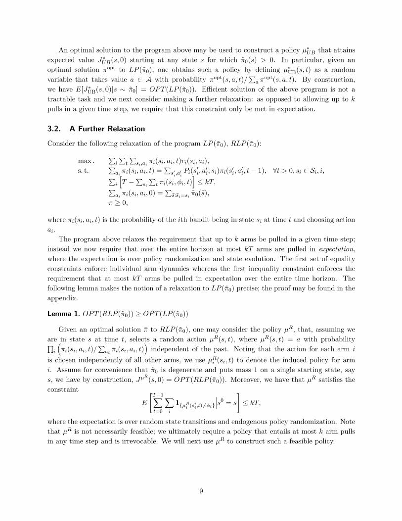
An optimal solution to the program above may be used to construct a policy µ∗UB that attainsexpected value J∗UB(s, 0) starting at any state s for which π0(s) > 0. In particular, given anoptimal solution πopt to LP (π0), one obtains such a policy by defining µ∗UB(s, t) as a randomvariable that takes value a ∈ A with probability πopt(s, a, t)/

∑a π

opt(s, a, t). By construction,we have E[J∗UB(s, 0)|s ∼ π0] = OPT (LP (π0)). Efficient solution of the above program is not atractable task and we next consider making a further relaxation: as opposed to allowing up to kpulls in a given time step, we require that this constraint only be met in expectation.

3.2. A Further Relaxation

Consider the following relaxation of the program LP (π0), RLP (π0):

max .∑i

∑t

∑si,ai πi(si, ai, t)ri(si, ai),

s. t.∑ai πi(si, ai, t) =

∑s′i,a′iPi(s′i, a′i, si)πi(s′i, a′i, t− 1), ∀t > 0, si ∈ Si, i,∑

i

[T −

∑si

∑t πi(si, φi, t)

]≤ kT,∑

ai πi(si, ai, 0) =∑s:si=si π0(s),

π ≥ 0,

where πi(si, ai, t) is the probability of the ith bandit being in state si at time t and choosing actionai.

The program above relaxes the requirement that up to k arms be pulled in a given time step;instead we now require that over the entire horizon at most kT arms are pulled in expectation,where the expectation is over policy randomization and state evolution. The first set of equalityconstraints enforce individual arm dynamics whereas the first inequality constraint enforces therequirement that at most kT arms be pulled in expectation over the entire time horizon. Thefollowing lemma makes the notion of a relaxation to LP (π0) precise; the proof may be found in theappendix.

Lemma 1. OPT (RLP (π0)) ≥ OPT (LP (π0))

Given an optimal solution π to RLP (π0), one may consider the policy µR, that, assuming weare in state s at time t, selects a random action µR(s, t), where µR(s, t) = a with probability∏i

(πi(si, ai, t)/

∑ai πi(si, ai, t)

)independent of the past. Noting that the action for each arm i

is chosen independently of all other arms, we use µRi (si, t) to denote the induced policy for armi. Assume for convenience that π0 is degenerate and puts mass 1 on a single starting state, says, we have by construction, JµR(s, 0) = OPT (RLP (π0)). Moreover, we have that µR satisfies theconstraint

E

[T−1∑t=0

∑i

1µRi (sti,t) 6=φi

∣∣∣s0 = s

]≤ kT,

where the expectation is over random state transitions and endogenous policy randomization. Notethat µR is not necessarily feasible; we ultimately require a policy that entails at most k arm pullsin any time step and is irrevocable. We will next use µR to construct such a feasible policy.

9

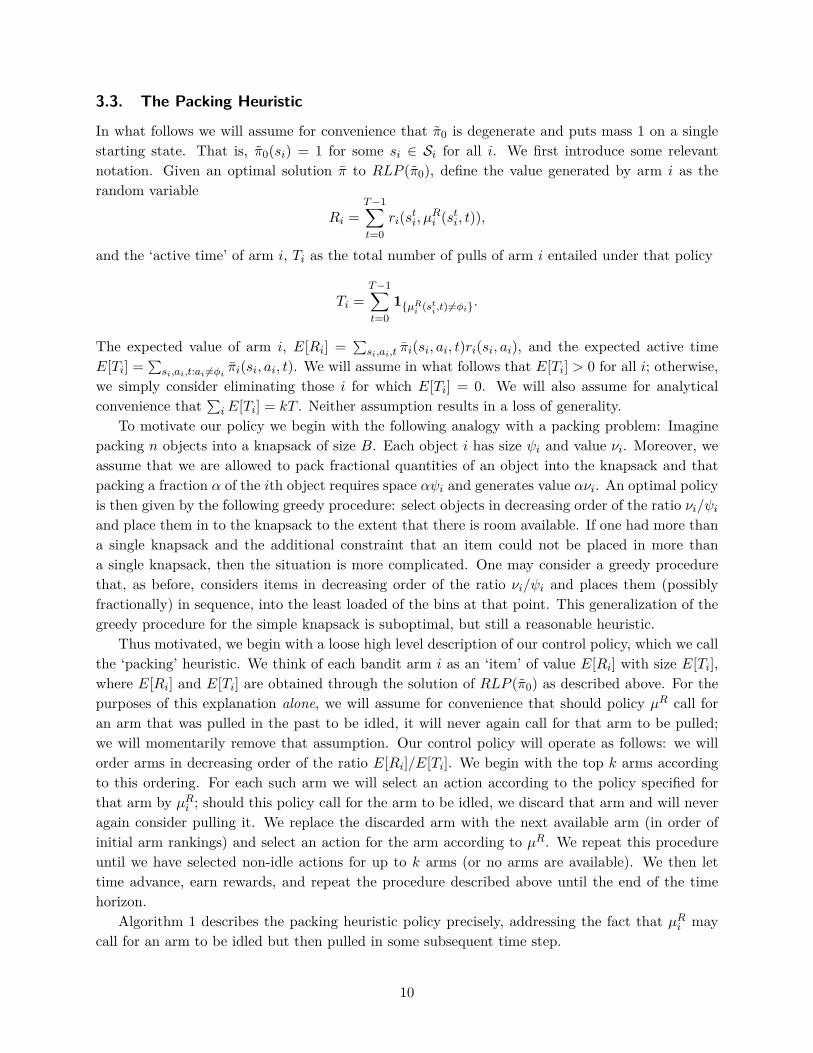
3.3. The Packing Heuristic

In what follows we will assume for convenience that π0 is degenerate and puts mass 1 on a singlestarting state. That is, π0(si) = 1 for some si ∈ Si for all i. We first introduce some relevantnotation. Given an optimal solution π to RLP (π0), define the value generated by arm i as therandom variable

Ri =T−1∑t=0

ri(sti, µRi (sti, t)),

and the ‘active time’ of arm i, Ti as the total number of pulls of arm i entailed under that policy

Ti =T−1∑t=0

1µRi (sti,t) 6=φi.

The expected value of arm i, E[Ri] =∑si,ai,t πi(si, ai, t)ri(si, ai), and the expected active time

E[Ti] =∑si,ai,t:ai 6=φi πi(si, ai, t). We will assume in what follows that E[Ti] > 0 for all i; otherwise,

we simply consider eliminating those i for which E[Ti] = 0. We will also assume for analyticalconvenience that

∑iE[Ti] = kT . Neither assumption results in a loss of generality.

To motivate our policy we begin with the following analogy with a packing problem: Imaginepacking n objects into a knapsack of size B. Each object i has size ψi and value νi. Moreover, weassume that we are allowed to pack fractional quantities of an object into the knapsack and thatpacking a fraction α of the ith object requires space αψi and generates value ανi. An optimal policyis then given by the following greedy procedure: select objects in decreasing order of the ratio νi/ψiand place them in to the knapsack to the extent that there is room available. If one had more thana single knapsack and the additional constraint that an item could not be placed in more thana single knapsack, then the situation is more complicated. One may consider a greedy procedurethat, as before, considers items in decreasing order of the ratio νi/ψi and places them (possiblyfractionally) in sequence, into the least loaded of the bins at that point. This generalization of thegreedy procedure for the simple knapsack is suboptimal, but still a reasonable heuristic.

Thus motivated, we begin with a loose high level description of our control policy, which we callthe ‘packing’ heuristic. We think of each bandit arm i as an ‘item’ of value E[Ri] with size E[Ti],where E[Ri] and E[Ti] are obtained through the solution of RLP (π0) as described above. For thepurposes of this explanation alone, we will assume for convenience that should policy µR call foran arm that was pulled in the past to be idled, it will never again call for that arm to be pulled;we will momentarily remove that assumption. Our control policy will operate as follows: we willorder arms in decreasing order of the ratio E[Ri]/E[Ti]. We begin with the top k arms accordingto this ordering. For each such arm we will select an action according to the policy specified forthat arm by µRi ; should this policy call for the arm to be idled, we discard that arm and will neveragain consider pulling it. We replace the discarded arm with the next available arm (in order ofinitial arm rankings) and select an action for the arm according to µR. We repeat this procedureuntil we have selected non-idle actions for up to k arms (or no arms are available). We then lettime advance, earn rewards, and repeat the procedure described above until the end of the timehorizon.

Algorithm 1 describes the packing heuristic policy precisely, addressing the fact that µRi maycall for an arm to be idled but then pulled in some subsequent time step.

10

Algorithm 1 The Packing Heuristic1: Renumber bandits so that E[R1]

E[T1] ≥E[R2]E[T2] · · · ≥

E[Rn]E[Tn] . Index bandits by variable i.

2: li ← 0, ai ← φi for all i, s ∼ π0(·)The ‘local time’ of every arm is set to 0 and its designated action to the idle action. An initialstate is drawn according to the initial state distribution π0.

3: J ← 0 Total reward earned is initialized to 0.4: X← 1, 2, . . . , k,A← k + 1, . . . , n,D = ∅.

Initialize the set of active (X), available (A), and discarded (D) arms.5: for t = 0 to T − 1 do6: while there exists an arm i ∈ X with ai = φi do Select up to k arms to pull.7: Select an i ∈ X with ai = φi

In what follows, either select an action for arm i or else discard it.8: while ai = φi and li < T do Attempt to select a pull action for arm i9: Select ai ∝ πi(si, ·, li) Select an action according to the solution to RLP (π).

10: li ← li + 1 Increment arm i’s local time.11: end while12: if li = T and ai = φi then Discard arm i and activate next highest ranked arm available.13: X← X \ i,D← D ∪ i Discard arm i.14: if A 6= ∅ then There are available arms.15: j ← min A Select highest ranked available arm.16: X← X ∪ j,A← A \ j Add arm to active set.17: end if18: end if19: end while20: for Every i ∈ X do Pull selected arms.21: si ∼ P (si, ai, ·)

Pull arm i; select next arm i state according to its transition kernel assuming the use ofaction ai.

22: J ← J + ri(si, ai) Earn rewards.23: ai ← φi24: end for25: end for

11

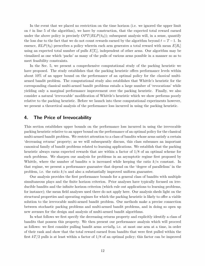
In the event that we placed no restriction on the time horizon (i.e. we ignored the upper limiton t in line 5 of the algorithm), we have by construction, that the expected total reward earnedunder the above policy is precisely OPT (RLP (π0)); subsequent analysis will, in a sense, quantifythe loss due to the fact that we do not count rewards earned by the algorithm beyond t = T −1. Inessence, RLP (π0) prescribes a policy wherein each arm generates a total reward with mean E[Ri]using an expected total number of pulls E[Ti], independent of other arms. Our algorithm may bevisualized as one which ‘packs’ as many of the pulls of various arms possible in a manner so as tomeet feasibility constraints.

In the Sec. 5, we present a comprehensive computational study of the packing heuristic wehave proposed. The study establishes that the packing heuristic offers performance levels withinabout 10% of an upper bound on the performance of an optimal policy for the classical multi-armed bandit problem. The computational study also establishes that Whittle’s heuristic for thecorresponding classical multi-armed bandit problems entails a large number of ‘revocations’ whileyielding only a marginal performance improvement over the packing heuristic. Finally, we alsoconsider a natural ‘irrevocable’ modification of Whittle’s heuristic which we show performs poorlyrelative to the packing heuristic. Before we launch into these computational experiments however,we present a theoretical analysis of the performance loss incurred in using the packing heuristic.

4. The Price of Irrevocability

This section establishes upper bounds on the performance loss incurred in using the irrevocablepacking heuristic relative to an upper bound on the performance of an optimal policy for the classicalmulti-armed bandit problem. We restrict attention to a class of bandits whose arms satisfy a certain‘decreasing returns’ property; as we will subsequently discuss, this class subsumes an importantcanonical family of bandit problems related to learning applications. We establish that the packingheuristic always earns expected rewards that are within a factor of 1/8 of an optimal scheme forsuch problems. We sharpen our analysis for problems in an asymptotic regime first proposed byWhittle, where the number of bandits n is increased while keeping the ratio k/n constant. Inthat regime, we present a performance guarantee that depend on the ‘degree of parallelism’ in theproblem, i.e. the ratio k/n and also a substantially improved uniform guarantee.

Our analysis provides the first performance bounds for a general class of bandits with multiplesimultaneous plays and the finite horizon criterion. Prior analyses have typically focused on irre-ducible bandits and the infinite horizon criterion (which rule out applications to learning problems,for instance); the mean field analyses used there do not apply here. Our analysis sheds light on thestructural properties and operating regimes for which the packing heuristic is likely to offer a viablesolution to the irrevocable multi-armed bandit problem. Our methods make a precise connectionbetween stochastic packing problems and multi-armed bandit problems, and in doing so open upnew avenues for the design and analysis of multi-armed bandit algorithms.

In what follows we first specify the decreasing returns property and explicitly identify a class ofbandits that possess this property. We then present our performance analysis which will proceedas follows: we first consider pulling bandit arms serially, i.e. at most one arm at a time, in orderof their rank and show that the total reward earned from bandits that were first pulled within thefirst kT/2 pulls is at least within a factor of 1/8 of an optimal policy; this factor can be improved

12

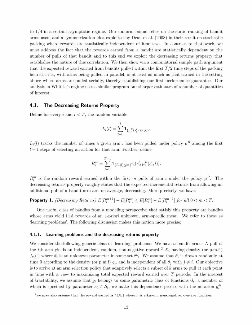
to 1/4 in a certain asymptotic regime. Our uniform bound relies on the static ranking of banditarms used, and a symmetrization idea exploited by Dean et al. (2008) in their result on stochasticpacking where rewards are statistically independent of item size. In contrast to that work, wemust address the fact that the rewards earned from a bandit are statistically dependent on thenumber of pulls of that bandit and to this end we exploit the decreasing returns property thatestablishes the nature of this correlation. We then show via a combinatorial sample path argumentthat the expected reward earned from bandits pulled within the first T/2 time steps of the packingheuristic i.e., with arms being pulled in parallel, is at least as much as that earned in the settingabove where arms are pulled serially, thereby establishing our first performance guarantee. Ouranalysis in Whittle’s regime uses a similar program but sharper estimates of a number of quantitiesof interest.

4.1. The Decreasing Returns Property

Define for every i and l < T , the random variable

Li(l) =l∑

t=01µRi (sti,t)6=φi

.

Li(l) tracks the number of times a given arm i has been pulled under policy µR among the firstl + 1 steps of selecting an action for that arm. Further, define

Rmi =T−1∑l=0

1Li(l)≤mri(sli, µ

Ri (sli, l)).

Rmi is the random reward earned within the first m pulls of arm i under the policy µR. Thedecreasing returns property roughly states that the expected incremental returns from allowing anadditional pull of a bandit arm are, on average, decreasing. More precisely, we have:

Property 1. (Decreasing Returns) E[Rm+1i ]− E[Rmi ] ≤ E[Rmi ]− E[Rm−1

i ] for all 0 < m < T .

One useful class of bandits from a modeling perspective that satisfy this property are banditswhose arms yield i.i.d rewards of an a-priori unknown, arm-specific mean. We refer to these as‘learning problems’. The following discussion makes this notion more precise:

4.1.1. Learning problems and the decreasing returns property

We consider the following generic class of ‘learning’ problems: We have n bandit arms. A pull ofthe ith arm yields an independent, random, non-negative reward 2 Xi having density (or p.m.f.)fθi(·) where θi is an unknown parameter in some set Θi. We assume that θi is drawn randomly attime 0 according to the density (or p.m.f) gi, and is independent of all θj with j 6= i. Our objectiveis to arrive at an arm selection policy that adaptively selects a subset of k arms to pull at each pointin time with a view to maximizing total expected reward earned over T periods. In the interestof tractability, we assume that gi belongs to some parametric class of functions Gi, a member ofwhich is specified by parameter si ∈ Si; we make this dependence precise with the notation gsii .

2we may also assume that the reward earned is h(Xi) where h is a known, non-negative, concave function.

13

Moreover, we assume that gsii is a conjugate prior for fθi for all si ∈ Si. That is, our posterior onθi given an observation Xi remains in Gi.

Learning problems of this type are rather common and fit a number of modeling needs, includingfor instance, the fast fashion and call-center staffing examples described in the introduction (seeCaro and Gallien (2007), Arlotto et al. (2009), and also Section 5 for concrete examples withinthis framework). In addition, these problems are in a sense the canonical application of the banditmodel (see Bellman (1956), Gittins and Wang (1992)). For further applications see the booksBergman and Gittins (1985); Berry and Fristedt (1985).

It is not hard to see that the learning problem we have posed can be cast as a multi-armedbandit problem in the sense of the model in Section 3. In particular, the state space for each arm issimply Si, with action space Ai = pi, φi consisting of two actions – pull and idle. The transitionkernel Pi is specified implicitly by Bayes’ rule and the reward function is defined according to:

ri(si, pi) =∫x,θxfθi(x)g

sii (θi)dθidx

By Bayes’ rule, rewards from a given arm (as defined above) will then satisfy the following intuitiveproperty reflecting the consistency of our estimate of the mean reward from a bandit arm:

ri(si, pi) =∑s′i∈Si

Pi(si, p, s′i)ri(s′i, pi), ∀si ∈ Si.

In light of the following Lemma, this broad class of learning problems satisfy the decreasingreturns property. In particular, we have the following result whose proof may be found in theappendix:

Lemma 2. Given a multi-armed bandit problem with Ai = pi, φi ∀i, and

ri(si, pi) ≥∑s′i∈Si

Pi(si, pi, s′i)ri(s′i, pi), ∀i, si ∈ Si,

we must haveE[Rm+1

i ]− E[Rmi ] ≤ E[Rmi ]− E[Rm−1i ]

for all 0 < m < T .

4.2. A Uniform Bound on the Price of Irrevocability

For convenience of exposition we assume that T is even; addressing the odd case requires essentiallyidentical proofs but cumbersome notation.

We re-order the bandits in decreasing order of E[Ri]/E[Ti] as in the packing heuristic. Let usdefine

H∗ = min

j :j∑i=1

E[Ti] ≥ kT/2

.Thus, H∗ is the set of bandits that take up approximately half the budget on total expected pulls.Next, let us define for all i ≤ H∗, random variables Ri and Ti according to Ri = Ri, Ti = Ti for all

i < H∗ and RH∗ = αRH∗ and TH∗ = αTH∗ , where α = kT/2−∑H∗−1i=1 E[Ti]

E[TH∗ ].

14

We begin with a preliminary lemma whose proof may be found in the appendix:

Lemma 3.H∗∑i=1

E[Ri] ≥12OPT (RLP (π0)).

We next compare the expected reward earned by a certain subset of bandits with indices nolarger than H∗. The significance of the subset of bandits we define will be seen later in the proofof Lemma 6 – we will see there that all bandits in this subset will begin operation prior to timeT/2 in a run of the packing heuristic. In particular, define

R1/2 =H∗∑i=1

1∑i−1j=1 Tj<kT/2

Ri.

Lemma 4.E[R1/2] ≥

14OPT (RLP (π0)).

Proof. We have:

E[R1/2](a)=

H∗∑i=1

Pr

i−1∑j=1

Tj < kT/2

E[Ri]

(b)≥

H∗∑i=1

Pr

i−1∑j=1

Tj < kT/2

E[Ri]

(c)=H∗∑i=1

Pr

i−1∑j=1

Tj < kT/2

E[Ri]

(d)≥

H∗∑i=1

(1−

∑i−1j=1E[Tj ]kT/2

)E[Ri]

=H∗∑i=1

E[Ri]−H∗∑i=1

∑i−1j=1E[Tj ]kT/2

E[Ri]

(e)≥

H∗∑i=1

E[Ri]−12

H∗∑i=1

∑H∗j=1,j 6=iE[Tj ]kT/2

E[Ri]

(f)≥ 1

2

H∗∑i=1

E[Ri]

(g)≥ 1

4OPT (RLP (π0))

Equality (a) follows from the fact that under policy µR, Ri is independent of Tj for j < i. In-equality (b) follows from our definition of Ri: Ri ≤ Ri. Equality (c) follows from the fact that bydefinition Ti = Ti for all i < H∗. Inequality (d) invokes Markov’s inequality.

Inequality (e) is the critical step in establishing the result and uses the simple symmetrizationidea exploited by Dean et al. (2008): In particular, we observe that since E[Ri]

E[Ti] ≤E[Rj ]E[Tj ] for i >

j, it follows that E[Ri]E[Tj ] ≤ 12(E[Ri]E[Tj ] + E[Rj ]E[Ti]) for i > j. Replacing every term

of the form E[Ri]E[Tj ] (with i > j) in the expression preceding inequality (e) with the upper

15

bound 12(E[Ri]E[Tj ] + E[Rj ]E[Ti]) yields inequality (e). Inequality (f) follows from the fact that∑H∗

i=1E[Ti] = kT/2 and since E[Ri] ≥ 0. Inequality (g) follows from Lemma 3.

Before moving on to our main Lemma that translates the above guarantees to a guarantee onthe performance of the packing heuristic, we need to establish one additional technical fact. Recallthat Rmi is the reward earned by bandit i in the first m pulls of this bandit under policy µR. Also,note that RTi = Ri. Exploiting the assumed decreasing returns property, we have the followingLemma whose proof may be found in the appendix:

Lemma 5. For bandits satisfying the decreasing returns property (Property 1),

E

[H∗∑i=1

1∑i−1j=1 Tj<kT/2

RT/2i

]≥ 1

2E[R1/2].

We have thus far established estimates for total expected rewards earned assuming implicitlythat bandits are pulled in a serial fashion in order of their rank. The following Lemma connects theseestimates to the expected reward earned under the µpacking policy (given by the packing heuristic)using a simple sample path argument. In particular, the following Lemma shows that the expectedrewards under the µpacking policy are at least as large as E

[∑H∗i=1 1∑i−1

j=1 Tj<kT/2RT/2i

].

Lemma 6. Assuming π0(s) = 1, we have

Jµpacking(s, 0) ≥ E

[H∗∑i=1

1∑i−1j=1 Tj<kT/2

RT/2i

].

Proof. For a given sample path of the system define

h = (H∗) ∧min

i :i∑

j=1Tj ≥ kT/2

.On this sample path, it must be that:

(1)H∗∑i=1

1∑i−1j=1 Tj<kT/2

RT/2i =

h∑i=1

RT/2i .

We claim that arms 1, 2, . . . , h are all first pulled at times t < T/2 under µpacking. Assume tothe contrary that this were not the case and recall that arms are considered in order of index underµpacking, so that an arm with index i is pulled for the first time no later than the first time arm l

is pulled for l > i. Let h′ be the highest arm index among the arms pulled at time t = T/2− 1 sothat h′ < h. It must be that

∑h′j=1 Tj ≥ kT/2. But then,

H∗ ∧min

i :i∑

j=1Tj ≥ kT/2

≤ h′which is a contradiction.

16

Thus, since every one of the arms 1, 2, . . . , h is first pulled at times t < T/2, each such arm maybe pulled for at least T/2 time steps prior to time T (the horizon). Consequently, we have that thetotal rewards earned on this sample path under policy µpacking are at least

h∑i=1

RT/2i

Using identity (1) and taking an expectation over sample paths yields the result.

We are ready to establish our main Theorem that provides a uniform bound on the performanceloss incurred in using the packing heuristic policy relative to an optimal policy with no restrictionson exploration. In particular, we have that the price of irrevocability is uniformly bounded forbandits satisfying the decreasing returns property.

Theorem 1. For multi-armed bandits satisfying the decreasing returns property (Property 1), wehave

Jµpacking(s, 0) ≥ 1

8J∗(s, 0)

Proof. We have from Lemmas 4,5 and 6 that

Jµpacking(s, 0) ≥ 1

8OPT (RLP (π0))

where π0(s) = 1. We know from Lemma 1 that OPT (RLP (π0)) ≥ OPT (LP (π0)) = J∗(s, 0) fromwhich the result follows.

4.3. The Price of Irrevocability in Whittle’s Asymptotic Regime

This section considers an asymptotic parameter regime where one may establish a stronger boundthan that in Theorem 1. In particular, the regime we will consider is a natural candidate forwhat one might consider a ‘large-scale’ problem. We are given an ‘unscaled’ problem with n0 armsin which we are allowed up to k0 simultaneous plays over a time horizon of T . We will assumethat each of these n0 arms have identical specifications and start in identical states; this is not anessential assumption but doing away with it does not permit a clean exposition. We next considera sequence of problems indexed by N , where the Nth problem has N copies of each of the n0 armsin the unscaled problem, and we allow Nk0 simultaneous plays over T time periods. Our goal is tounderstand the price of irrevocability as N gets large. Notice that this regime is still relevant forlearning problems since we are not scaling the time horizon, T , and are not restricting the kernelsPi in any way. This regime is analogous to one considered by Whittle (1988) and Weber and Weiss(1990), albeit for irreducible bandit problems and the average reward criterion (which rules outlearning applications, for instance). The finite horizon criterion and the fact that the bandits weconsider may be (and, for learning applications, will be) non-irreducible rule out the mean-fieldanalysis techniques of Weber and Weiss (1990).

Letting Ri,N and Ti,N denote the value generated by arm i and its active time (as defined inthe previous section) for the Nth problem, the following facts are apparent by our assumption thateach bandit is identical:

17

1. Ri,Nd=Ri,N ′ , and Ti,N

d=Ti,N ′ for all N,N ′ and i ≤ min(n0N,n0N′).

2. For every N , the collection of random variables R1,N , R2,N , . . . , Rn0N,N are i.i.d. as are therandom variables T1,N , T2,N , . . . , Tn0N,N .

3. E[Ti,N ] = k0T/n0 for all N and i ≤ n0N .

In light of the above facts we will eliminate the subscript N from Ri,N and Ti,N . We note thenthat for the Nth problem, OPT (RLP (π0)) =

∑Nn0i=1 E[Ri].

We prove two main bounds in this section:

1. We first present a performance guarantee that illustrates a dependence on the ratio k0/n0.This ratio may be interpreted as the ‘degree of parallelism’ inherent to the multi-armed banditproblem at hand.

2. We then prove a performance guarantee that holds in an asymptotic regime where N getslarge (but is otherwise uniform over problem parameters). This bound improves the boundin Theorem 1 by a factor of 2.

4.3.1. Impact of the ‘Degree of Parallelism’ (k0/n0)

Let us define the random variable τN = minj :∑ji=1 Ti ≥ k0NT. We then have the following

Lemma.

Lemma 7. In the N th system, all arms with indices smaller than or equal to τN ∧ n0N beginoperation prior to time T . Moreover, for any ε > 0 and almost all ω ∈ Ω, ∃N ε(ω), such that

τN ≥ Nn0 − (1 + ε)√Nn0 log logNn0

for all N ≥ N ε(ω).

The above Lemma is proved in the appendix. The Lemma is remarkable in that it states thatfor large scale problems (i.e. large N), almost all bandits begin operation prior to the end of thetime horizon. We next translate this fact to a bound on performance. To this end, for every N ,let σN (·) denote a (random) permutation of 1, . . . , Nn0 satisfying Ri > Rj =⇒ σ(i) < σ(j).Further, for every l ≤ Nn0, define the random variable

MN (l) =∑

i:σ(i)≤lRi

MN (l) is thus the realized reward of the top l arms assuming the packing heuristic were notterminated at the end of the time horizon. Define for α ∈ [0, 1],

γN (α) = E[MN (dNn0αe)]/E

Nn0∑i=1

Ri

.Since the Ri are i.i.d random variables, limN γN (α) , γ(α) is well defined by the law of largenumbers and is naturally interpreted as the ratio between the expected contribution of an arm

18

restricted to realizations that are in the top α fractile and the expected contribution of an arm.We then have the following result theorem indicates the impact of the ‘degree of parallelism’ in theproblem on the performance of the heuristic:

Theorem 2.

limN→∞

Jµpacking

N (s, 0)J∗N (s, 0)

≥ 1− γ(min(k0/n0, 1− k0/n0))

The above bound (which is established in the appendix) provides an indication of the role playedby the ratio k0/n0. Loosely, it may be interpreted as stating that the performance loss incurred bythe packing heuristic is no more than the relative contribution from the top k0/n0 percent of arms.While one may characterize the γ function given the distribution of rewards from a given arm Ri,a fair criticism of this bound is that it is difficult to characterize γ given only primitive problemdata. The next bound we provide will be uniform over problems parameters and valid for problemsin Whittle’s asymptotic regime.

4.3.2. A Uniform Guarantee for Whittle’s Regime

We present here a performance guarantee for the asymptotic regime under consideration thatdepends only on problem primitives (and is, in fact, uniform over this regime). The program wewill follow is essentially identical to that we followed for our proof of a uniform bound with theexception of Lemma 4; we prove an alternative result below allowing for a dependence on problemscale N . The proof may be found in the appendix.

Lemma 8. For the N th bandit problem, we have:

E[R1/2] ≥12(1− κ(N))OPT (RLP (π0)).

where κ(N) = O(N−1/2+d) and d > 0 is arbitrary.

Using the result of the previous Lemma (in place of Lemma 4), and Lemmas 5 and 6 we havethat

Theorem 3. For the N th multi-armed bandit problem,

Jµpacking(s, 0) ≥ 1

4(1− κ(N))J∗(s, 0)

where κ(N) = O(N−1/2+d) for arbitrary d > 0 and we assume si = sj ∀i, j.

This bound while still lose, provides a substantial improvement over the uniform bound in theprevious section. Together, Theorems 2 and 3 indicate that the packing heuristic is likely to performwell in Whittle’s asymptotic regime.

5. Computational Experiments

This section presents a computational investigation of the performance of the packing heuristic forthe irrevocable multi-armed bandit problem with a view to gauge its practical efficacy. We also

19

examine as an alternative heuristic for the irrevocable bandit problem, a natural modification toWhittle’s heuristic. Finally, we examine the performance of Whittle’s (non-irrevocable) heuristicitself, paying special attention to the number of arm ‘revocations’ under that heuristic. In addition,we benchmark the performance of all of these schemes against a computable upper bound on theexpected reward for any policy (with no restrictions on revocability); specifically, the bound is givenby the objective function of problem LP (π0) in Sec. 3.2 for an optimal solution3. We consider anumber of large scale bandit problems drawn from a generative family of problems to be discussedshortly, and demonstrate the following:

• The packing heuristic consistently demonstrates performance within about 10 to 20 % of anupper bound on the performance of an optimal policy for the classical multi-armed banditproblem. This upper bound is also an upper bound to the performance of any irrevocablescheme.

• The number of ‘revocations’ under Whittle’s heuristic can be large in a variety of operatingregimes. A natural modification to Whittle’s heuristic making it feasible for the irrevocablebandit problem typically performs 15 to 20 percent worse than Whittle’s heuristic in theseregimes. The packing heuristic can recover a substantial portion of the above gap (between50 and 100 %) in most cases.

The Generative Model: We consider multi-armed bandit problems with n arms up to k ofwhich may be pulled simultaneously at any time. The ith arm corresponds to a Binomial(m,Pi)random variable where m is fixed and known, and Pi is unknown but drawn from a Beta(αi, βi)prior distribution. Assuming we choose to ‘pull’ arm i at some point, we realize a random outcomeMi ∈ 0, 1, . . . ,m. Mi is a Binomial(m,Pi) random variable where Pi is itself a Beta(αi, βi) randomvariable. We receive a reward of riMi and update the prior distribution parameters according toαi ← αi + Mi, βi ← βi + m − Mi. By selecting the initial values of αi and βi for each armappropriately we can control for the initial level of uncertainty in the value of Pi; by ‘level ofuncertainty’ we mean the co-efficient of variation of Pi which is defined according to σ(Pi)/E[Pi].This model is applicable to the dynamic assortment selection problem studied in Caro and Gallien(2007) with each arm representing a product of uncertain popularity and Mi representing theuncertain number of product i sales over a single period in which that product is offered for sale;the only difference with that work is that as opposed to assuming Binomial demand, the authorsthere assume Poisson demand.

5.1. IID Bandits

We consider bandits with (n, k) ∈ (500, 75), (500, 125), (100, 15), (100, 25). These dimensions arerepresentative of large scale applications such as the dynamic assortment problem (see Caro andGallien (2007)). For each value of (n, k) we consider time horizons T = 40, 25 and 10 (again, horizonlengths of 40 and 25 reflect the dynamic assortment applications, assuming weekly restockingdecisions). We consider three different values for the coefficient of variation in arm bias: cv =1, 2.5, 4. These coefficients of variation represent respectively, a low, moderate and high degree

3The problem LP (π0) for both computation of the upper bound and the packing heuristic is solved with a toleranceof 10−6; the computational algorithm is described in the next section.

20

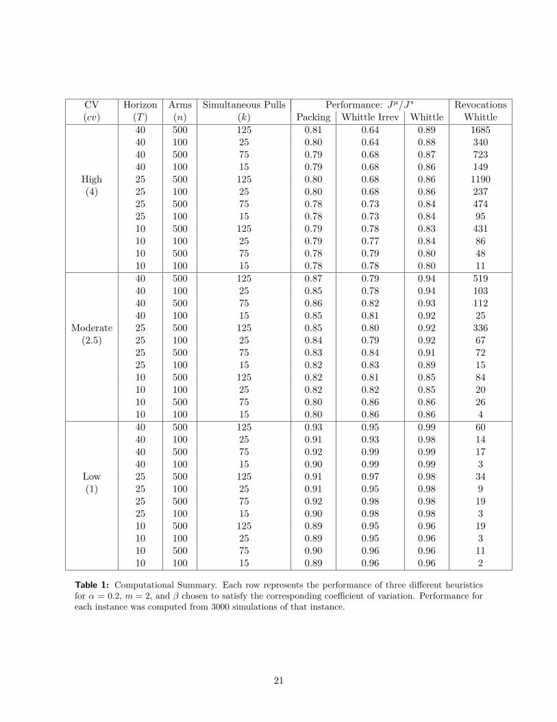
CV Horizon Arms Simultaneous Pulls Performance: Jµ/J∗ Revocations(cv) (T ) (n) (k) Packing Whittle Irrev Whittle Whittle

40 500 125 0.81 0.64 0.89 168540 100 25 0.80 0.64 0.88 34040 500 75 0.79 0.68 0.87 72340 100 15 0.79 0.68 0.86 149

High 25 500 125 0.80 0.68 0.86 1190(4) 25 100 25 0.80 0.68 0.86 237

25 500 75 0.78 0.73 0.84 47425 100 15 0.78 0.73 0.84 9510 500 125 0.79 0.78 0.83 43110 100 25 0.79 0.77 0.84 8610 500 75 0.78 0.79 0.80 4810 100 15 0.78 0.78 0.80 1140 500 125 0.87 0.79 0.94 51940 100 25 0.85 0.78 0.94 10340 500 75 0.86 0.82 0.93 11240 100 15 0.85 0.81 0.92 25

Moderate 25 500 125 0.85 0.80 0.92 336(2.5) 25 100 25 0.84 0.79 0.92 67

25 500 75 0.83 0.84 0.91 7225 100 15 0.82 0.83 0.89 1510 500 125 0.82 0.81 0.85 8410 100 25 0.82 0.82 0.85 2010 500 75 0.80 0.86 0.86 2610 100 15 0.80 0.86 0.86 440 500 125 0.93 0.95 0.99 6040 100 25 0.91 0.93 0.98 1440 500 75 0.92 0.99 0.99 1740 100 15 0.90 0.99 0.99 3

Low 25 500 125 0.91 0.97 0.98 34(1) 25 100 25 0.91 0.95 0.98 9

25 500 75 0.92 0.98 0.98 1925 100 15 0.90 0.98 0.98 310 500 125 0.89 0.95 0.96 1910 100 25 0.89 0.95 0.96 310 500 75 0.90 0.96 0.96 1110 100 15 0.89 0.96 0.96 2

Table 1: Computational Summary. Each row represents the performance of three different heuristicsfor α = 0.2, m = 2, and β chosen to satisfy the corresponding coefficient of variation. Performance foreach instance was computed from 3000 simulations of that instance.

21

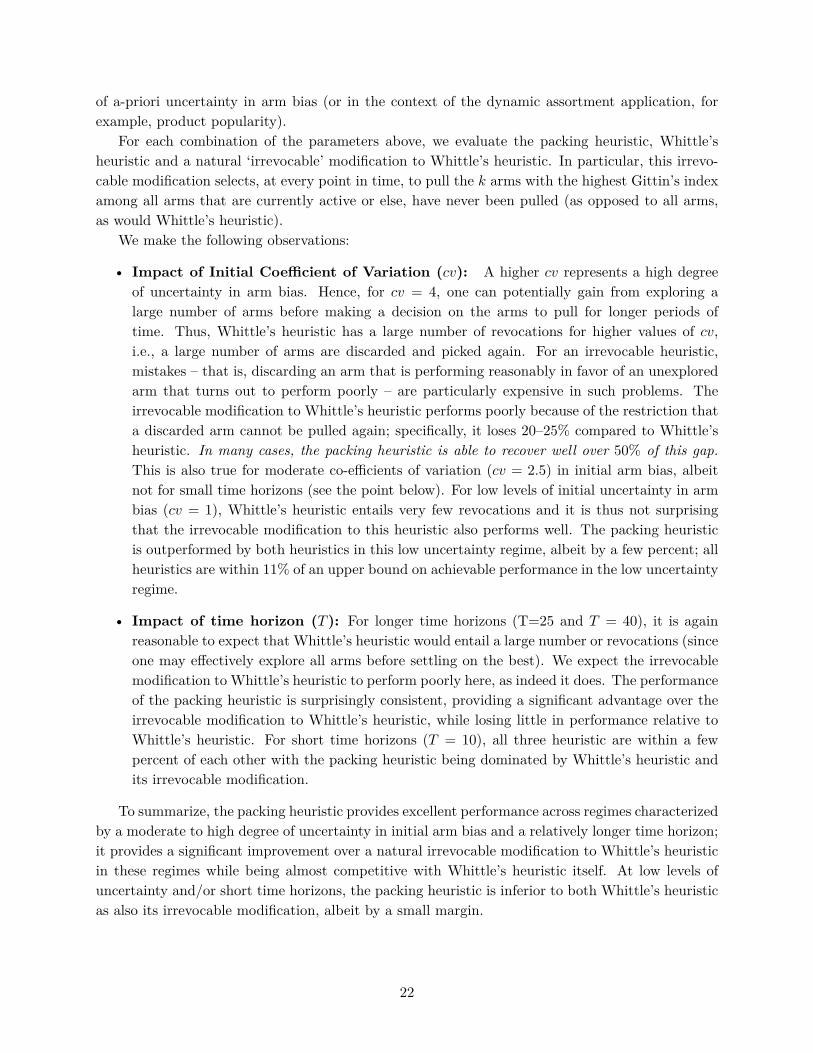
of a-priori uncertainty in arm bias (or in the context of the dynamic assortment application, forexample, product popularity).

For each combination of the parameters above, we evaluate the packing heuristic, Whittle’sheuristic and a natural ‘irrevocable’ modification to Whittle’s heuristic. In particular, this irrevo-cable modification selects, at every point in time, to pull the k arms with the highest Gittin’s indexamong all arms that are currently active or else, have never been pulled (as opposed to all arms,as would Whittle’s heuristic).

We make the following observations:

• Impact of Initial Coefficient of Variation (cv): A higher cv represents a high degreeof uncertainty in arm bias. Hence, for cv = 4, one can potentially gain from exploring alarge number of arms before making a decision on the arms to pull for longer periods oftime. Thus, Whittle’s heuristic has a large number of revocations for higher values of cv,i.e., a large number of arms are discarded and picked again. For an irrevocable heuristic,mistakes – that is, discarding an arm that is performing reasonably in favor of an unexploredarm that turns out to perform poorly – are particularly expensive in such problems. Theirrevocable modification to Whittle’s heuristic performs poorly because of the restriction thata discarded arm cannot be pulled again; specifically, it loses 20–25% compared to Whittle’sheuristic. In many cases, the packing heuristic is able to recover well over 50% of this gap.This is also true for moderate co-efficients of variation (cv = 2.5) in initial arm bias, albeitnot for small time horizons (see the point below). For low levels of initial uncertainty in armbias (cv = 1), Whittle’s heuristic entails very few revocations and it is thus not surprisingthat the irrevocable modification to this heuristic also performs well. The packing heuristicis outperformed by both heuristics in this low uncertainty regime, albeit by a few percent; allheuristics are within 11% of an upper bound on achievable performance in the low uncertaintyregime.

• Impact of time horizon (T ): For longer time horizons (T=25 and T = 40), it is againreasonable to expect that Whittle’s heuristic would entail a large number or revocations (sinceone may effectively explore all arms before settling on the best). We expect the irrevocablemodification to Whittle’s heuristic to perform poorly here, as indeed it does. The performanceof the packing heuristic is surprisingly consistent, providing a significant advantage over theirrevocable modification to Whittle’s heuristic, while losing little in performance relative toWhittle’s heuristic. For short time horizons (T = 10), all three heuristic are within a fewpercent of each other with the packing heuristic being dominated by Whittle’s heuristic andits irrevocable modification.

To summarize, the packing heuristic provides excellent performance across regimes characterizedby a moderate to high degree of uncertainty in initial arm bias and a relatively longer time horizon;it provides a significant improvement over a natural irrevocable modification to Whittle’s heuristicin these regimes while being almost competitive with Whittle’s heuristic itself. At low levels ofuncertainty and/or short time horizons, the packing heuristic is inferior to both Whittle’s heuristicas also its irrevocable modification, albeit by a small margin.

22

Horizon Arms Simultaneous Pulls Performance: Jµ/J∗ Revocations(T ) (n) (k) Packing Whittle Irrev Whittle Whittle40 501 125 0.91 0.80 0.92 198340 99 25 0.91 0.80 0.92 38940 501 75 0.88 0.80 0.91 105540 99 15 0.88 0.79 0.90 21425 501 125 0.90 0.83 0.92 137625 99 25 0.88 0.82 0.92 26425 501 75 0.87 0.83 0.90 69925 99 15 0.88 0.83 0.89 14210 501 125 0.89 0.90 0.92 32210 99 25 0.88 0.90 0.91 5910 501 75 0.85 0.86 0.87 12010 99 15 0.83 0.88 0.88 26

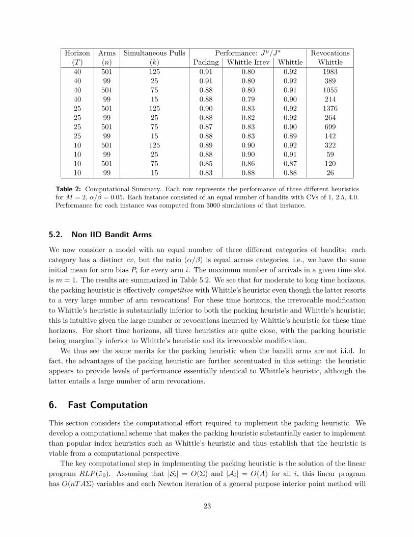
Table 2: Computational Summary. Each row represents the performance of three different heuristicsfor M = 2, α/β = 0.05. Each instance consisted of an equal number of bandits with CVs of 1, 2.5, 4.0.Performance for each instance was computed from 3000 simulations of that instance.

5.2. Non IID Bandit Arms

We now consider a model with an equal number of three different categories of bandits: eachcategory has a distinct cv, but the ratio (α/β) is equal across categories, i.e., we have the sameinitial mean for arm bias Pi for every arm i. The maximum number of arrivals in a given time slotis m = 1. The results are summarized in Table 5.2. We see that for moderate to long time horizons,the packing heuristic is effectively competitive with Whittle’s heuristic even though the latter resortsto a very large number of arm revocations! For these time horizons, the irrevocable modificationto Whittle’s heuristic is substantially inferior to both the packing heuristic and Whittle’s heuristic;this is intuitive given the large number or revocations incurred by Whittle’s heuristic for these timehorizons. For short time horizons, all three heuristics are quite close, with the packing heuristicbeing marginally inferior to Whittle’s heuristic and its irrevocable modification.

We thus see the same merits for the packing heuristic when the bandit arms are not i.i.d. Infact, the advantages of the packing heuristic are further accentuated in this setting: the heuristicappears to provide levels of performance essentially identical to Whittle’s heuristic, although thelatter entails a large number of arm revocations.

6. Fast Computation

This section considers the computational effort required to implement the packing heuristic. Wedevelop a computational scheme that makes the packing heuristic substantially easier to implementthan popular index heuristics such as Whittle’s heuristic and thus establish that the heuristic isviable from a computational perspective.

The key computational step in implementing the packing heuristic is the solution of the linearprogram RLP (π0). Assuming that |Si| = O(Σ) and |Ai| = O(A) for all i, this linear programhas O(nTAΣ) variables and each Newton iteration of a general purpose interior point method will

23

require O((nTAΣ)3

)steps. An interior point method that exploits the fact that bandit arms are

coupled via a single constraint will require O(n(TAΣ)3) computational steps at each iteration. Wedevelop a combinatorial scheme to solve this linear program that is in spirit similar to the classicalDantzig-Wolfe dual decomposition algorithm. In contrast with Dantzig-Wolfe decomposition, ourscheme is efficient. In particular, the scheme requires O(nTAΣ2 log(kT )) computational stepsto solve RLP (π0) making it a significantly faster solution alternative to the schemes alluded toabove. Equipped with this fast scheme, it is notable that using the packing heuristic requiresO(nAΣ2 log(kT )) computations per time step amortized over the time horizon which will typicallybe substantially less than the O(nAΣ2T ) computations required per time step for index policyheuristics such as Whittle’s heuristic.

Our scheme employs a ‘dual decomposition’ of RLP (π0). The key technical difficulty wemust overcome in developing our computational scheme for the solution of RLP (π0) is the non-differentiability of the dual function corresponding to RLP (π0) at an optimal dual solution whichprevents us from recovering an optimal or near optimal policy by direct minimization of the dualfunction.

6.1. An Overview of the Scheme

For each bandit arm i, define the polytope Di(π0) ∈ R|Si||Ai|T of permissible state-action frequenciesfor that bandit arm specified via the constraints of RLP (π0) relevant to that arm.

A point within this polytope, πi, corresponds to a set of valid state-action frequencies for theith bandit arm. With some abuse of notation, we denote the expected reward from this arm underπi by the ‘value’ function:

Ri(πi) =T−1∑t=0

πi(si, ai, t)ri(si, ai).

In addition denote the expected number of pulls of bandit arm i under πi by

Ti(πi) = T −∑si

∑t

πi(si, φi, t).

We understand that both Ri(·) and Ti(·) are defined over the domain Di(π0).We may thus rewrite RLP (π0) in the following form:

(2) max .∑iRi(πi),

s. t.∑i Ti(πi) ≤ kT.

The Lagrangian dual of this program is DRLP (π0):

min . λkT +∑i maxπi (Ri(πi)− λTi(πi)) ,

s. t. λ ≥ 0.

The above program is convex. In particular, the objective is a convex function of λ. We willshow that strong duality applies to the dual pair of programs above, so that the optimal solutionto the two programs have identical value. Next, we will observe that for a given value of λ, it issimple to compute maxπi (Ri(πi)− λTi(πi)) via the solution of a dynamic program over the state

24

space of arm i (a fast procedure). Finally it is simple to derive useful a-priori lower and upperbounds on the optimal dual solution λ∗. Thus, in order to solve the dual program, one may simplyemploy a bisection search over λ. Since for a given value of λ, the objective may be evaluatedvia the solution of n simple dynamic programs, the overall procedure of solving the dual programDRLP (π0) is fast.

What we ultimately require is the optimal solution to the primal program RLP (π0). Onenatural way we might hope to do this (that ultimately will not work) is the following: Havingcomputed an optimal dual solution λ∗, one may hope to recover an optimal primal solution, π∗

(which is what we ultimately want), via the solution of the problem

(3) maxπi

(Ri(πi)− λ∗Ti(πi)) .

for each i. This is the typical dual decomposition procedure. Unfortunately, this last step neednot necessarily yield a feasible solution to RLP (π0). In particular, solving (3) for λ = λ∗ + ε mayresult in an arbitrarily suboptimal solution for any ε > 0, while solving (3) for a λ ≤ λ∗ mayyield an infeasible solution to RLP (π0). The technical reason for this is that the Lagrangian dualfunction for RLP (π) may be non-differentiable at λ∗. These difficulties are far from pathological,and Example 1 illustrates how they may arise in a very simple example.

Example 1. The following example illustrates that the dual function may be non-differentiable atan optimal solution, and that it is not sufficient to solve (3) for λ ≤ λ∗ or λ = λ∗ + ε for an ε > 0arbitrarily small. Specifically, consider the case where we have n = 2 identical bandits, T = 1, andK = 1. Each bandit starts in state s, and two actions can be chosen for it, namely, a and theidling action φ. The rewards are r(s, a) = 1 and r(s, φ) = 0. Thus, RLP (π0) for this specific caseis given by:

max . π1(s, a, 0) + π2(s, a, 0),s. t. π1(s, a, 0) + π2(s, a, 0) ≤ 1,

where πi ∈ Di(π0), i = 1, 2. Clearly, the optimal objective function value for the above optimizationproblem is 1. The Lagrangian dual function for the above problem is

g(λ) = λ+ maxπ1(s,a,0)

π1(s, a, 0)(1− λ) + maxπ2(s,a,0)

π2(s, a, 0)(1− λ)

=

2− λ λ ≤ 1λ λ > 1

Not the dual function is minimized at λ∗ = 1, which is a point of non-differentiability. Moreover,solving (3) at λ∗ + ε for any ε > 0, gives π1(s, a, 0) = π2(s, a, 0) = 0 which is clearly suboptimal.Also, a solution for 0 ≤ λ ≤ λ∗ is π1(s, a, 0) = π2(s, a, 0) = 1, which is clearly infeasible.

Notice that in the above example, the average of the solutions to problem (3) for λ = λ∗− ε andλ = λ∗+ε does yield a feasible, optimal primal solution, π1(s, a, 0) = π2(s, a, 0) = 1/2. We overcomethe difficulties presented by the non-differentiability of the dual function by computing both upperand lower approximations to λ∗, and computing solutions to (3) for both of these approximations.We then consider as our candidate solution to RLP (π0), a certain convex combination of the twosolutions. In particular, we propose algorithm 2, that takes as input the specification of the bandit

25

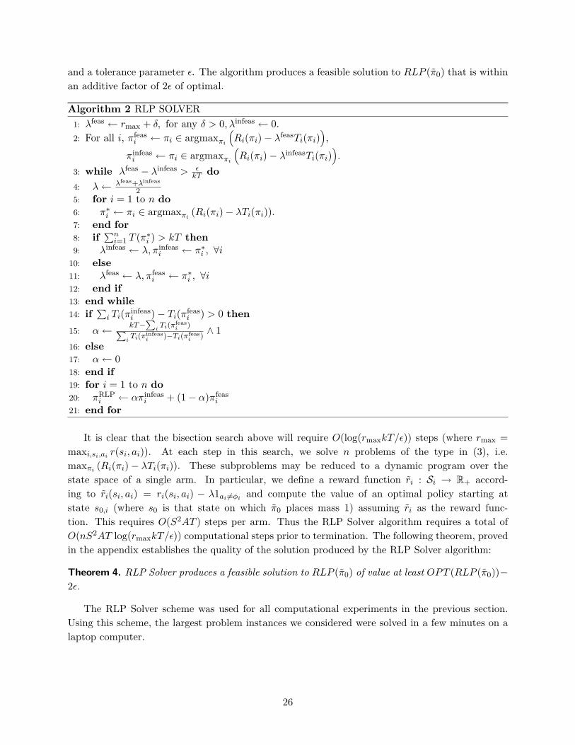
and a tolerance parameter ε. The algorithm produces a feasible solution to RLP (π0) that is withinan additive factor of 2ε of optimal.

Algorithm 2 RLP SOLVER1: λfeas ← rmax + δ, for any δ > 0, λinfeas ← 0.2: For all i, πfeas

i ← πi ∈ argmaxπi(Ri(πi)− λfeasTi(πi)

),

πinfeasi ← πi ∈ argmaxπi

(Ri(πi)− λinfeasTi(πi)

).

3: while λfeas − λinfeas > εkT do

4: λ← λfeas+λinfeas

25: for i = 1 to n do6: π∗i ← πi ∈ argmaxπi (Ri(πi)− λTi(πi)).7: end for8: if

∑ni=1 T (π∗i ) > kT then

9: λinfeas ← λ, πinfeasi ← π∗i , ∀i

10: else11: λfeas ← λ, πfeas

i ← π∗i , ∀i12: end if13: end while14: if

∑i Ti(πinfeas

i )− Ti(πfeasi ) > 0 then

15: α← kT−∑iTi(πfeas

i )∑iTi(πinfeas

i )−Ti(πfeasi ) ∧ 1

16: else17: α← 018: end if19: for i = 1 to n do20: πRLP

i ← απinfeasi + (1− α)πfeas

i

21: end for

It is clear that the bisection search above will require O(log(rmaxkT/ε)) steps (where rmax =maxi,si,ai r(si, ai)). At each step in this search, we solve n problems of the type in (3), i.e.maxπi (Ri(πi)− λTi(πi)). These subproblems may be reduced to a dynamic program over thestate space of a single arm. In particular, we define a reward function ri : Si → R+ accord-ing to ri(si, ai) = ri(si, ai) − λ1ai 6=φi and compute the value of an optimal policy starting atstate s0,i (where s0 is that state on which π0 places mass 1) assuming ri as the reward func-tion. This requires O(S2AT ) steps per arm. Thus the RLP Solver algorithm requires a total ofO(nS2AT log(rmaxkT/ε)) computational steps prior to termination. The following theorem, provedin the appendix establishes the quality of the solution produced by the RLP Solver algorithm:

Theorem 4. RLP Solver produces a feasible solution to RLP (π0) of value at least OPT (RLP (π0))−2ε.

The RLP Solver scheme was used for all computational experiments in the previous section.Using this scheme, the largest problem instances we considered were solved in a few minutes on alaptop computer.

26

7. Concluding Remarks

This paper introduced the ‘irrevocable’ multi-armed bandit problem as a practical model withinwhich to design policies for a number of interesting learning applications. We have developed a newalgorithm for this problem – the packing heuristic – that we have shown performs quite well andis practical for large scale deployment. In particular, we have presented a thorough performanceanalysis that has yielded uniform approximation performance guarantees as well as guarantees thatillustrate a dependence on problem parameters. We have also presented an extensive computationalstudy to support what the theory suggests. In the interest of performance, we have presented a fastimplementation of the packing heuristic that is faster than schemes that rely on the computationof Gittins indices.

Perhaps the single most useful outcome of this work has been to show that irrevocability is notnecessarily an expensive constraint. This fact is supported by both our theory and computationalexperiments for a general class of learning applications. While natural ‘irrevocable’ modifications toschemes that perform well for the classical multi-armed bandit problem (such as Whittles heuristic)may not necessarily achieve this goal, the scheme we provide – the packing heuristic - does.

In addition, the theoretical analysis we provide has indirectly yielded the first performancebounds for an important general class of multi-armed bandit problems that to this point have hadsurprisingly little theoretical attention. More importantly, the new mode of analysis these problemshave called for reveals a tantalizing connection with stochastic packing problems. This paper hasfurthered that connection.

Moving forward, we anticipate two research directions emerging from the present work. First,it would be interesting to further explore the connection with stochastic packing problems. Thereexists a vast body of algorithmic work for such problems, and it would be interesting to see whatthis yields for multi-armed bandit problems. A second direction is exploring the requirementof irrevocability in the non-parametric bandit setting; it is clear that an irrevocable scheme cannever be regret optimal. The question to ask is how sub-optimal from a regret perspective can anirrevocable scheme be made in the non-parasmetric setting.

ReferencesAnantharam, V., P. Varaiya, J. Walrand. 1987a. Asymptotically efficient allocation rules for the multiarmed

bandit problem with multiple plays-part i: I.i.d. rewards. Automatic Control, IEEE Transactions on 32(11)968–976.

Anantharam, V., P. Varaiya, J. Walrand. 1987b. Asymptotically efficient allocation rules for the multiarmedbandit problem with multiple plays-part II: Markovian rewards. Automatic Control, IEEE Transactionson 32(11) 977–982.

Anscombe, F. J. 1963. Sequential medical trials. Journal of the American Statistical Association 58(302)365–383.

Arlotto, A, S Chick, N. Gans. 2009. Hiring and retention of heterogeneous workers. Working Paper.

Armitage, P., G. Berry, J. N. S. Matthews. 2002. Statistical methods in medical research. 4th ed. Wiley-Blackwell.

27

Bellman, R. E. 1956. A problem in the sequential design of experiments. Sakhya Ser. A 30 221–252.

Bergman, S. W, J.C. Gittins. 1985. Statistical methods for pharmaceutical research planning, vol. 67. M.Dekker.

Berry, D. A, B. Fristedt. 1985. Bandit problems: sequential allocation of experiments. Monographs onstatistics and applied probability, Chapman and Hall.

Bertsimas, D., J. Nino-Mora. 2000. Restless bandits, linear programming relaxations, and a primal-dualindex heuristic. Operations Research 48(1) 80–90.

Bhattacharjee, R., A. Goel, S. Khanna, B. Null. 2007. The ratio index for budgeted learning, with applica-tions. Working Paper .

Boyd, S., L. Vandenberghe. 2004. Convex Optimization. Cambridge University Press.

Caro, F., J. Gallien. 2007. Dynamic assortment with demand learning for seasonal consumer goods. Man-agement Science 53 276–292.

Dean, B.C., M.X. Goemans, J. Vondrak. 2008. Approximating the stochastic knapsack problem: The benefitof adaptivity. Mathematics of Operations Research 33(4) 945–964.

Gittins, J, Y. G. Wang. 1992. The learning component of dynamic allocation indices. The Annals of Statistics20(3) 1625–1636.

Gittins, J.C. 1989. Multi-armed Bandit Allocation Indices. Wiley.

Gittins, J.C., D.M. Jones. 1974. A dynamic allocation index for the sequential design of experiments. 241–266.

Glazebrook, K. D., D. J. Wilkinson. 2000. Index-based policies for discounted multi-armed bandits on parallelmachines. The Annals of Applied Probability 10(3) 877–896.

Guha, S., K. Munagala. 2007. Approximation algorithms for budgeted learning problems. STOC ’07:Proceedings of the thirty-ninth annual ACM symposium on Theory of computing. ACM, New York, NY,USA, 104–113.

Lai, T., H. Robbins. 1985. Asymptotically efficient adaptive allocation rules. Advances in Applied Mathematic6(1) 4–22.

Pich, M. T, L. Van der Heyden. 2002. Marks & spencer and zara: Process competition in the textile apparelindustry. INSEAD Business Case Study.

Shor, N.Z. 1985. Minimization Methods for Non-differentiable Functions. Springer-Verlag.

Weber, R. R., G. Weiss. 1990. On an index policy for restless bandits. Journal of Applied Probability 27(3)637–648.

Whittle, P. 1988. Restless bandits: Activity allocation in a changing world. Journal of Applied Probability25 287–298.

28

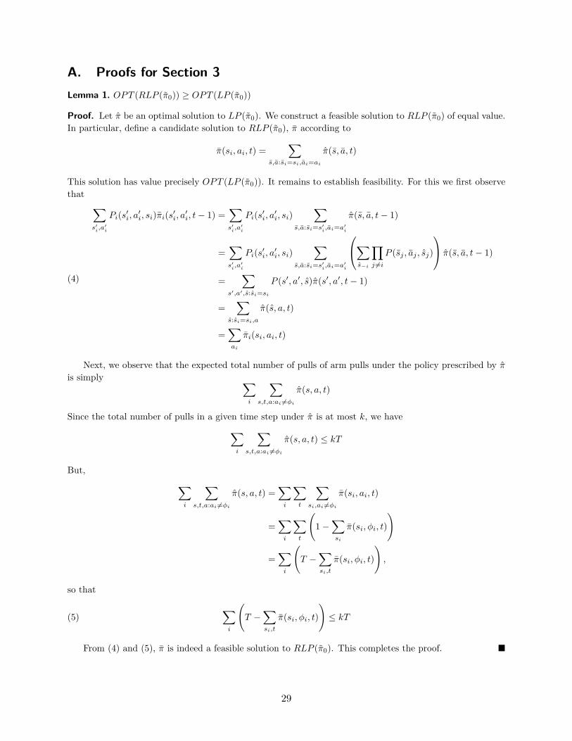
A. Proofs for Section 3Lemma 1. OPT (RLP (π0)) ≥ OPT (LP (π0))

Proof. Let π be an optimal solution to LP (π0). We construct a feasible solution to RLP (π0) of equal value.In particular, define a candidate solution to RLP (π0), π according to

π(si, ai, t) =∑

s,a:si=si,ai=ai

π(s, a, t)

This solution has value precisely OPT (LP (π0)). It remains to establish feasibility. For this we first observethat ∑

s′i,a′i

Pi(s′i, a′i, si)πi(s′i, a′i, t− 1) =∑s′i,a′i

Pi(s′i, a′i, si)∑

s,a:si=s′i,ai=a′i

π(s, a, t− 1)

=∑s′i,a′i

Pi(s′i, a′i, si)∑

s,a:si=s′i,ai=a′i

∑s−i

∏j 6=i

P (sj , aj , sj)

π(s, a, t− 1)

=∑

s′,a′,s:si=si

P (s′, a′, s)π(s′, a′, t− 1)

=∑

s:si=si,aπ(s, a, t)

=∑ai

πi(si, ai, t)

(4)

Next, we observe that the expected total number of pulls of arm pulls under the policy prescribed by πis simply ∑

i

∑s,t,a:ai 6=φi

π(s, a, t)

Since the total number of pulls in a given time step under π is at most k, we have∑i

∑s,t,a:ai 6=φi

π(s, a, t) ≤ kT

But, ∑i

∑s,t,a:ai 6=φi

π(s, a, t) =∑i

∑t

∑si,ai 6=φi

π(si, ai, t)

=∑i

∑t

(1−

∑si

π(si, φi, t)

)

=∑i

(T −

∑si,t

π(si, φi, t)

),

so that

(5)∑i

(T −

∑si,t

π(si, φi, t)

)≤ kT

From (4) and (5), π is indeed a feasible solution to RLP (π0). This completes the proof.

29

B. Proofs for Section 4Lemma 2. Given a multi-armed bandit problem with Ai = pi, φi ∀i, and

ri(si, pi) ≥∑s′i∈Si

Pi(si, pi, s′i)ri(s′i, pi), ∀i, si ∈ Si,

we must haveE[Rm+1

i ]− E[Rmi ] ≤ E[Rmi ]− E[Rm−1i ]

for all 0 < m < T .

Proof. We first introduce some notation. It is clear that the policy µRi induces a Markov process on thestate space Si. We expand this state space, so as to track the total number of arm pulls so that our statespace now become Si×T ∪T. The policy µRi induces a distribution over arm i states for every time t < T ,which we denote by the variable π. Thus, π(si,m, t, ai) will denote the probability of being in state (si,m)at time t and taking action ai.

Now,E[Rm+1

i −Rmi ] =∑si,t<T

π(si,m, t, pi)ri(si, pi)

and similarly, for E[Rmi −Rm−1i ].

But,

∑si,t<T

π(si,m, t, pi)ri(si, pi) =∑

si,t<T−1π(si,m− 1, t, pi)

∑s′i

Pi(si, pi, s′i)h(s′i, t+ 1)ri(s′i, pi)

≤

∑si,t<T−1

π(si,m− 1, t, pi)

∑s′i

Pi(si, pi, s′i)ri(s′i, pi)

≤

∑si,t<T−1

π(si,m− 1, t, pi)ri(si, pi)

≤∑si,t<T

π(si,m− 1, t, pi)ri(si, pi)

= E[Rmi −Rm−1i ]

where h(si, t) = 1 −∏T−1t′=t Pr(µRi (si, t′) = φi). Here

∏T−1t′=t Pr(µRi (si, t′) = φi) is the probability of never

pulling the arm after reaching state si at time t so that h(si, t) represents the probability of eventuallypulling arm i after reaching state si at time t. The second inequality follows from the assumption on rewardstructure in the statement of the Lemma. We thus see that coins satisfy the decreasing returns property.

Lemma 4.H∗∑i=1

E[Ri] ≥12OPT (RLP (π0)).

Proof. For t ≥ 0, define a function

f(t) =n∑i=1

E[Ri]E[Ti]

t− i−1∑j=1

E[Ti]

+

∧ E[Ti]

,

where (a ∧ b) = min(a, b) and (x)+ = x if x ≥ 0, and 0 otherwise. By construction (i.e. since E[Ri]E[Ti] is

30

non-increasing in i), we have that f is a concave function on [0, kT ]. Now observe that

H∗∑i=1

E[Ri] =H∗−1∑i=1

E[Ri]E[Ti]

E[Ti] +E[RH∗ ]E[TH∗ ]

kT/2− H∗−1∑j=1

E[Ti]

= f(kT/2).

Next, observe that

OPT (RLP (π0)) =n∑i=1

E[Ri]E[Ti]

E[Ti] = f(kT ).

By the concavity of f and since f(0) = 0, we have that f(kT/2) ≥ 12f(kT ), which yields the result.

Lemma 5. For bandits satisfying the decreasing returns property (Property 1),

E

[H∗∑i=1

1∑i−1j=1

Tj<kT/2RT/2i

]≥ 1

2E[R1/2].

Proof. We note that assuming Property 1 implies that E[RT/2i ] ≥ 12E[Ri] for all i. The assertion of the

Lemma is then evident – in particular,

E[R1/2] =H∗∑i=1

Pr

i−1∑j=1

Tj < kT/2

E[Ri]

≤H∗∑i=1

Pr

i−1∑j=1

Tj < kT/2

2E[RT/2i ]

= 2E

[H∗∑i=1

1∑i−1j=1

Tj<kT/2RT/2i

]

where the first and second equality use the fact that Ri and RT/2i are each independent of Tj for j 6= i.

Lemma 7. In the N th system, all arms with indices smaller than or equal to τN ∧n0N begin operation priorto time T . Moreover, for any ε > 0 and almost all ω ∈ Ω, ∃N ε(ω), such that

τN ≥ Nn0 − (1 + ε)√Nn0 log logNn0

for all N ≥ N ε(ω).

Proof. We begin with noting that for any ε > 0 and almost all ω ∈ Ω, ∃N ε(ω), such that

(6)m∑i=1

Ti ≤ mk0T/n0 + (1 + ε)√m log logmk0T/n0

for all m ≥ N ε(ω). This is immediate from the Law of the Iterated Logarithm for i.i.d random variables.Now, let us denote m(N) = Nn0 − (1 + ε)

√Nn0 log logNn0. Notice that

m(N)k0T/n0 + (1 + ε)√m(N) log logm(N)k0T/n0 ≤ Nk0T.

Thus, by (6), it follows thatm(N)∑i=1

Ti ≤ Nk0T

31

eventually. But then it must be thatτn ≥ m(N)

eventually, which yields the second part of the Lemma. Now, for the first part of the Lemma, assume forthe sake of contradiction that the highest indexed arm pulled up to time T − 1 has an index (say, l) smallerthan τN ∧ n0N . That is, this assumption would imply that there exists an l < τN ∧ n0N satisfying

l∑i=1

Ti ≥ Nk0T.

But then, τN ≤ l which yields a contradiction and thus the result.

Theorem 2.

limN→∞

Jµpacking

N (s, 0)J∗N (s, 0)

≥ 1− γ(min(k0/n0, 1− k0/n0))

Proof. From Lemma 7, it follows that in the Nth system at least τN ∧ n0N bandits begin operation priorto time T , i.e. the end of the horizon. Now since at most k0N arms can be active at any point in time, itmust then be that

Jµpacking

N (s, 0) ≥ E

[τn∧n0N∑i=1

Ri −Mτn∧n0N (k0N)

]

≥ E

[τn∧n0N∑i=1

Ri −Mn0N (k0N)

]

We also have

Jµpacking

N (s, 0) ≥ E

[k0N∑i=1

Ri

]≥ E

[n0N∑i=1

Ri −Mn0N ((n0 − k0)N)

]

≥ E

[τn∧n0N∑i=1

Ri −Mn0N ((n0 − k0)N)

]

Now, limN

E[∑τN∧n0N

i=1Ri]

E[∑n0N

i=1Ri] = 1 (by Lemma 7, and since theRi are bounded) and J∗N (s, 0) ≤ E

[∑n0Ni=1 Ri

].

Thus, the above bounds, and the fact that γ(·) is non-decreasing yield:

limN→∞

Jµpacking

N (s, 0)J∗N (s, 0)

≥ 1− γ(k0/n0 ∧ 1− k0/n0).

Lemma 7. For the N th bandit problem, we have:

E[R1/2] ≥12(1− κ(N))OPT (RLP (π0)).

where κ(N) = O(N−1/2+d) and d > 0 is arbitrary.

Proof. Observe that for the Nth problem, H∗ =⌈k0NT/2k0T/n0

⌉=⌈Nn0

2⌉. We then have for the Nth problem

32

and an arbitrary ε > 0,

E[R1/2] =H∗∑i=1

Pr

i−1∑j=1

Tj < k0NT/2

E[Ri]

≥

⌊Nn0

2(1+ε)

⌋∑i=1

Pr

i−1∑j=1

Tj < k0NT/2

E[Ri].

Now, for i ≤⌊Nn0

2(1+ε)

⌋, we have that k0NT/2

ik0T/n0≥ 1 + ε. Now, for i ≤

⌊Nn0

2(1+ε)

⌋, we have:

Pr

i∑j=1

Tj < k0NT/2

= 1− Pr

i∑j=1

Tj ≥ k0NT/2

≥ 1− Pr

⌊Nn0

2(1+ε)

⌋∑j=1

Tj ≥ k0NT/2

≥ 1− Pr

⌊Nn0

2(1+ε)

⌋∑j=1

Tj ≥⌊

Nn0

2(1 + ε)

⌋k0T (1 + ε)/n0

= 1− Pr

⌊Nn0

2(1+ε)

⌋∑j=1

Tj − E[Tj ] ≥⌊

Nn0

2(1 + ε)

⌋εk0T/n0

≥ 1− exp

(−2k2

0/n20

⌊Nn0

2(1 + ε)

⌋ε2)

where the third inequality is Hoeffding’s inequality for independent random variables.Thus,

E[R1/2] ≥(

1− exp(−2k2

0/n20

⌊Nn0

2(1 + ε)

⌋ε2))⌊ Nn0

2(1+ε)

⌋∑i=1

E[Ri]

≥(

1− exp(−2k2

0/n20

⌊Nn0

2(1 + ε)

⌋ε2))(

11 + ε

)(Nn0 − 2Nn0 + 2

) H∗∑i=1

E[Ri]

≥(

1− exp(−2k2

0/n20

⌊Nn0

2(1 + ε)

⌋ε2))(

11 + ε

)(Nn0 − 2Nn0 + 2

)OPT (RLP (π0))

2

where the second inequality follows from the fact that H∗ =⌈Nn0

2⌉. By setting ε = N−1/2+d for d > 0,

arbitrarily small, we have the result.

C. Proof of Theorem 4The following lemma shows that the optimal objective function value of the dual is equal to OPT (RLP (π0)).In particular, it shows that Slater’s constraint qualification condition holds (see, for example, Boyd andVandenberghe (2004)).

33

Lemma 9. OPT (RLP (π0)) = OPT (DRLP (π0)). That is, strong duality holds.

Proof. To show this, it is sufficient to show that there is a strictly feasible solution to (2), i.e., the inequalityis satisfied strictly. This is straightforward – in particular, for each bandit i, set πi(si, φi, t) = π0,i(si) for allsi and t, where π0,i(si) is the probability of bandit i starting in state si. Set πi(si, ai, t) = 0 for ai 6= φi forall si, t. These state action frequencies belong to Di(π0), and also give Ti(πi) = 0.

We denote R∗ = OPT (RLP (π0)) = OPT (DRLP (π0)). Also, define the following set of total runningtimes for all bandits corresponding to a dual variable λ:

T (λ) =

∑i

Ti(πi)∣∣∣∣πi ∈ argmax

πi

(Ri(πi)− λTi(πi))), ∀i

.

Lemma 10. If 0 ≤ λ1 < λ2, thenmin T (λ1) ≥ max T (λ2).

Proof. We denote the objective function in DRLP (π0), i.e., the dual function by:

g(λ) = λkT +∑i

maxπi

(Ri(πi)− λTi(πi)) .

The slack in the total running time constraint∑i Ti(πi) ≤ kT , i.e. kT −

∑i T (πi), is a subgradient of g for

any π such that πi ∈ argmaxπi (Ri(πi)− λTi(πi)) (see Shor (1985)). Thus, the set of subgradients of thedual function g at λ are given by

∂g(λ) = kT − t : t ∈ T (λ).

Then, since g is a convex function, it follows that for 0 ≤ λ1 < λ2,

kT − t1 ≤ kT − t2, ∀ t1 ∈ T (λ1), t2 ∈ T (λ2).

The lemma then follows.

(π∗, λ∗) is an optimal solution for the primal and dual problems if and only if (see, for example, Boydand Vandenberghe (2004))

(7)π∗i ∈ argmax

πi

(Ri(πi)− λ∗Ti(πi)) ,

either λ∗ > 0 and∑i

Ti(π∗i ) = kT, or λ∗ = 0 and∑i

Ti(π∗i ) ≤ kT.

We prove the correctness of the RLP Solver algorithm separately for the cases when λ∗ = 0 is optimal,and when any optimal solution satisfies λ∗ > 0. We denote the values of the bounds on the dual variablethat are computed by the last iteration of the RLP solver algorithm by λfeas and λinfeas. Recall that,

πfeasi ∈ argmax

πi

(Ri(πi)− λfeasTi(πi)

),

πinfeasi ∈ argmax

πi

(Ri(πi)− λinfeasTi(πi)

).

We introduce some additional notation:

T feas =∑i

Ti(πfeasi ), Rfeas =

∑i

Ri(πfeasi ),

T infeas =∑i

Ti(πinfeasi ), Rinfeas =

∑i

Ri(πinfeasi ).

34

Thus,

(8)g(λfeas) = λfeaskT +Rfeas − λfeasT feas,

g(λinfeas) = λinfeaskT +Rinfeas − λfeasT infeas.

Lemma 11. If (π∗, λ∗) is a solution to (7) with λ∗ = 0, then

R∗ −(αRinfeas + (1− α)Rfeas) ≤ ε.

Proof. If λ∗ = 0, it follows from (7) that there is some t ∈ T (0) such that t ≤ kT . Hence, it follows fromLemma 10 that for any λ > 0, max T (λ) ≤ kT . Hence, Line 11 of the RLP solver algorithm is alwaysinvoked, and so, the RLP solver algorithm converges to

λinfeas = 0 and 0 < λfeas < ε/(kT ).

Hence, πinfeasi ∈ argmaxπi(Ri(πi)). Also, g(λ) is minimized at λ∗ = 0. Hence, it follows from Lemma 9 that

(9) R∗ = g(0) =∑i

maxπi

Ri(πi) = Rinfeas.

Since, λfeas > 0, it follows from T feas ≤ kT . Hence, we now consider the following three cases:

• Case 1: T infeas ≤ kT .Here, α = 1, and hence, using (9) it follows that

R∗ −(αRinfeas + (1− α)Rfeas) = 0.

• Case 2: T feas = kT .In this case, (πfeas, λfeas) satisfy the optimality conditions in (7). Thus, Rfeas = R∗, and so (sinceRinfeas = R∗ by (9))

R∗ −(αRinfeas + (1− α)Rfeas) = 0.

• Case 3: T infeas > kT > T feas.Since, g(λ) is minimized at λ = 0,

R∗ = g(0) ≤ g(λfeas) = λfeaskT +Rfeas − λfeasT feas

⇒ R∗ −Rfeas ≤ λfeas (kT − T feas) .Since, R∗ = Rinfeas (from (9)), and using the fact that 0 < α < 1 when T infeas > kT > T feas, we have

R∗ − αRinfeas − (1− α)Rfeas = (1− α)(R∗ −Rfeas)≤ (1− α)(kT − T feas)λfeas

≤ kTλfeas

≤ ε,

(10)

Lemma 12. If every solution to (7) satisfies λ∗ > 0, then

R∗ −(αRinfeas + (1− α)Rfeas) ≤ 2ε.

Proof. The RLP solver algorithm is initialized with λinfeas = 0. Since, λ∗ > 0, and (kT ) ∈ T (λ∗) ((7)), itfollows from Lemma 10 that min T (0) ≥ kT . But (kT ) /∈ T (0), else there would be a solution to (7) that

35

satisfies λ∗ = 0, leading to a contradiction. Thus, min T (0) > kT , and so lines 8–12 of the RLP solveralgorithm guarantee that

(11) T infeas > kT.

Using an appropriate modification of the optimality conditions in (7) for the case where the horizon is T infeas

(instead of kT ), we see that Rinfeas is the maximum reward earned by any policy in π :∑i Ti(πi) ≤ T infeas.

Since, R∗ is the maximum reward earned by any policy in π :∑i Ti(πi) ≤ kT < T infeas,

(12) Rinfeas ≥ R∗.

We now argue that T feas ≤ kT . The RLP solver algorithm is initialized with λfeas > rmax. Since,πfeasi ∈ argmaxπi

(Ri(πi)− λfeasTi(πi)

), initially, the optimal policy is to idle at all times. Thus, T feas ≤ kT

at initialization; at all other iterations, lines 8–12 of the algorithm ensure that T feas ≤ kT .We now consider the following two cases separately:

• Case 1: T feas = kT .In this case, (πfeas, λfeas) satisfy the optimality conditions in (7), and so, Rfeas = R∗. Now, using (12)(

αRinfeas + (1− α)Rfeas) ≥ R∗.• Case 2: T feas < kT .

Note that the RLP solver algorithm terminates when

(13) λfeas − λinfeas < ε/(kT ).

Now T feas < kT and (kT ) ∈ T (λ∗). If λfeas < λ∗, it follows from Lemma 10 that

T feas ≥ min T (λfeas) ≥ max T (λ∗) ≥ kT,

which is a contradiction. Hence,

(14) λfeas ≥ λ∗.

Also, since (kT ) ∈ T (λ∗), it follows from Lemma 10 that for any λ > λ∗, max T (λ) ≤ kT . So, (11)implies that

(15) λinfeas ≤ λ∗.

It follows from (13),(14),(15) that

max(0, λ∗ − ε

kT

)≤ λinfeas and λfeas ≤ λ∗ + ε

kT.

Since g(λ) is minimized at λ∗, it follows from (8) and strong duality proved in Lemma 9 that

g(λ∗) = R∗ ≤ g(λfeas) = Rfeas + λfeas (kT − T feas) ≤ Rfeas + (λ∗ + δ)(kT − T feas) ,

g(λ∗) = R∗ ≤ g(λinfeas) = Rinfeas + λinfeas (kT − T infeas) ≤ Rinfeas + (λ∗ − δ)(kT − T infeas) ,

where δ = ε/(kT ). Note that the above inequalities also use T feas < kT (by assumption) and T infeas >

36

kT (from (11)). Thus,

R∗ − αRinfeas − (1− α)Rfeas = α(R∗ −Rinfeas) + (1− α)(R∗ −Rfeas)≤ α(δ − λ∗)

(T infeas − kT

)+ (1− α)(λ∗ + δ)

(kT − T feas)

= 2δ(Tinfeas − kT )(kT − T feas)

T infeas − T feas

≤ 2δkT= 2ε.

Theorem 2. RLP Solver produce a feasible solution to RLP (π0) of value at least OPT (RLP (π0))− 2ε.

Proof. The result follows from Lemmas 11 and 12, and the fact that λ∗ ≥ 0 (from (7)).

37