Research Institute of Industrial Economics P.O. Box 55665

SE-102 15 Stockholm, Swedeninfo@ifn.sewww.ifn.se

IFN Working Paper No. 690, 2007 The Inventor’s Role: Was Schumpeter Right?

Pontus Braunerhjelm and Roger Svensson

1

The Inventor’s Role: Was Schumpeter Right?

Pontus Braunerhjelm * and Roger Svensson **

August 2008

Abstract According to Schumpeter, the creative process of economic development can be divided into the three distinguishable stages of invention, innovation (commercialization) and imitation. Following this theory, invention and innovation require different skills. This paper tests whether the invention and innovation stages should be undertaken by different agents. We also show why there is a rationale for the Schumpeterian entrepreneur to also include the inventor in the innovation process. Merging the two enhances the possibilities of successful commercialization since the inventor may further adapt the innovation to customer needs, transmit information and reduce uncertainty. This serves to expand the market opportunities for the entrepreneur. The empirical analysis is based on a survey covering Swedish patents granted to individuals and small firms. The results show that profitability increases by 21 percent when the patent is licensed or sold to an entrepreneur, or if the inventor is employed in an entrepreneurial firm, as compared to commercialization undertaken by the inventor. Another important result is that, irrespective of commercialization mode, an active involvement of the inventor is shown to have a positive impact on performance. Key words: Entrepreneur, inventor, innovations, commercialization.

JEL: 031, 032, M13 -------------------------------- * Leif Lundblad’s Chair in International Business and Entrepreneurship, The Royal School of Technology, Department of Transport and Economics, SE-100 44 Stockholm, Sweden. E-mail: pontusb@infra.kth.se ; Tel: +46 – 8 – 790 91 14; Fax: +46 – 8 – 790 95 17. ** Research Institute of Industrial Economics, P.O. Box 55665, SE-10215 Stockholm, Sweden. E-mail: roger.svensson@ifn.se ; Tel: +46 – 8 – 665 45 49; Fax: +46 – 8 – 665 45 99. The authors would like to thank Erik Mellander, Magnus Henrekson, Lars Persson and seminar participants at the annual EARIE conference in Valencia, the Max Planck Conference in Bangalore and the Oslo Entrepreneurship Workshop (where the paper was awarded the price of “Best paper in Entrepreneurship and Innovation”), for constructive comments. Jakob Eliasson provided excellent research assistance. The Bank of Sweden Tercentenary Foundation, Marianne and Marcus Wallenberg Foundation, and Torsten and Ragnar Söderberg’s Foundation are acknowledged for generous financial support. Finally, the paper has benefited from insightful comments in the referee process to this journal.

2

1. Introduction

Perhaps more than any other economist, Schumpeter (1911) is explicit about the economic

function of the entrepreneur. By introducing innovations to the market, the entrepreneur

distorts the prevailing equilibrium, challenges existing structures and sets industrial dynamics

and economic development into motion. According to Schumpeter, the process of economic

development can be divided into three clearly separate stages. The first stage implies technical

discovery of new things or new ways of doing things, which Schumpeter refers to as

invention. In the subsequent stage innovation occurs, i.e. the successful commercialization of

a new good or service stemming from technical discoveries or, more generally, a new

combination of knowledge (new and old). The final step in this three-stage process – imitation

– concerns a more general adoption and diffusion of new products or processes to markets.

For our purpose, the interesting part consists of the separation between the stages of

invention and innovation. Schumpeter (1947, p.149) himself claims that “the inventor

produces ideas, the entrepreneur ‘gets things done’ ….. an idea or scientific principle is not,

by itself, of any importance for economic practice.” Thus, Schumpeter views the creation of

technological opportunity as being basically outside the domain of the entrepreneur. Rather,

the identification and exploitation of such opportunities is what distinguishes entrepreneurs,

i.e., innovation. Nor did Schumpeter view entrepreneurs as risk-takers, even though he did not

completely dismiss the idea and was aware that innovation contains elements of risk also for

the entrepreneur. But basically, that task was attributed the capitalists who financed

entrepreneurial ventures.

This paper seeks to answer two questions associated with the way Schumpeter

disconnected inventions and innovators. The first is simply whether Schumpeter was right on

this issue and to what extent disconnecting the stages influences the success of

commercialization. Focusing on entrepreneurs and small firms, does invention and innovation

take place in independent units and to what extent is commercialization performance

influenced by the degree of integration of these activities? What are the strategic implications

for inventors that consider entering the market? Over the last decades, there are plenty of

examples of fast-growing entrepreneurial firms that are based on individuals’ inventions,

where Microsoft probably constitutes the most conspicuous case of a successful combination

of the inventor and innovator role. However, there is also ample evidence of the opposite.

Going back a few decades, but remaining within the same industry, William Shockley’s

invention known as the semiconductor was brilliant. Still, his company − Shockley’s

Semiconductors − performed less well but inspired several entrepreneurial employees who

later choose to leave and try their own inventive and innovative capabilities (the “traitorous

3

eight”). More recently, entrepreneurial firms like Google and e-Bay have implemented (and

refined) existing to technologies to exploit entrepreneurial opportunities. Thus, judging from

anecdotic evidence, there seem to be examples of both inventors and innovators that have

successfully commercialized new products.

The second question concerns the involvement of the inventor in the

commercialization process. More precisely, can we observe that entrepreneurs and small firms

that actively involve the inventor in the commercialization of new products are more

profitable? This is associated with the way inventive activities are organized, i.e. the degree of

vertical integration of inventive and innovative stages and access to complementary assets,

which can be traced to the environment in which they operate. In particular, the institutional

design and the structure of the market are decisive (Teece 1986). This issue has not been

empirically examined in the previous literature, with the exception of more explorative

studies.1

We argue that the integration of the two stages may, in fact, be considered part of

entrepreneurial ability as envisioned in the Schumpeter world. That is, reflecting the

“combinatorial capability” required for successful commercialization. It is also likely to

reduce uncertainty in entrepreneurial activities, as defined by Knight (1921), since

commercialization may also imply adaptation of the original invention to specific market and

firm conditions. Such adaptation is likely to rely on the private knowledge embodied in the

inventor. In addition, the entrepreneur also reduces the risks of being exposed to increased

competition from follow-up innovations by the inventor, or from other firms to which the

inventor may find it profitable to license an invention. In fact, this suggests a bridge between

Knight’s and Schumpeter’s approaches to entrepreneurship.

To empirically address these issues, we will implement a unique database on Swedish

patents granted to individuals and small firms. Data is collected through a survey with a

response rate of 80 percent. In particular, the database contains information about the extent

of commercialization of individual patents, whether the commercialization was successful and

the role of the inventor in the commercialization process. Using discrete statistical models, we

empirically examine how different explanatory factors (e.g., commercialization mode, firm

type, activity of inventors) affect the performance. To the best of our knowledge, such an

1 Taking all firms into account, irrespective of size, there has been a clear tendency in the 20th century towards an increased vertical integration of inventive (R&D) and producing activities according to for instance Teece (1988) and Aghion and Howitt (1998). Others challenge those findings and claim that technological progress and institutional changes have facilitated a vertically dispersed production structure (Arora et al. 2001; Grossman and Helpman 2002).

4

empirical analysis, where explanatory factors are related to the performance of patent

commercialization, has not previously been carried out. 2

The paper is organized as follows. Section 2 presents a brief discussion of the inventor

and the entrepreneur, drawing on previous insights in industrial organization theory, contract

theory and the strategic management literature. The database and basic statistics are described

in section 3. The statistical model is set up and explanatory variables are described in section

4. The empirical estimations are shown in section 5, and the final section concludes.

2. Entrepreneurs, invention and innovation

Most contemporary theories of entrepreneurship build on the seminal contributions by

Schumpeter (1911) who stressed the importance of innovative entrepreneurs as the main

vehicle to move an economy forward from static equilibrium, Knight’s (1921) proposed role

of the entrepreneur as someone who transforms uncertainty into a calculable risk and,

somewhat later, Kirzner’s (1973) view that the entrepreneur moves an economy towards

equilibrium (contrasting Schumpeter) by taking advantage of arbitrage possibilities. More

generally, the research field of entrepreneurship has recently been defined as analyses of

“how, by whom and with what consequences opportunities to produce future goods and

services are discovered, evaluated and exploited” (Shane and Venkataraman, 2000).3

As regards by “whom”, an eclectic definition of the entrepreneur, that has become

increasingly accepted, is suggested by Wennekers and Thurik (1999). The entrepreneur: i) is

innovative, i.e. perceives and creates new opportunities; ii) operates under uncertainty and

introduces products to the market, decides on location, and the form and use of resources; and

iii) manages his business and competes with others for a share of the market.4 Apparently, this

definition can be linked to all three contributions referred to above. Note that invention is not

explicitly mentioned (albeit creation of opportunity is) in this definition, nor excluded from

the interpretation of entrepreneurship. Thus, it deviates, but is not completely disentangled,

from Schumpeter’s (1911, p. 88-89 ) traditional view on innovation and invention:

“Economic leadership in particular must hence be distinguished from ‘invention’. As long as they are

not carried into practice, inventions are economically irrelevant. And to carry any improvement into effect is a

task entirely different from the inventing of it, and a task, moreover, requiring entirely different kinds of

aptitudes. Although entrepreneurs of course may be inventors just as they may be capitalists, they are inventors

2 In fact, Teece (2006) stress the importance of empirical research addressing precisely these issues. 3 A related strand of the literature focuses on differences in individual capabilities (Carroll and Hannan 2000), or the interaction between the characteristics of opportunity and the characteristics of the people who exploit them (Casson 2005). Schumpeter also considered individual’s psychological capacity as the key in identifying opportunities. 4 Here we adopt the somewhat modified version as introduced by Bianchi and Henrekson (2005).

5not by nature of their function but by coincidence and vice versa ... it is, therefore, not advisable, and it may be

downright misleading, to stress the element of inventions as much as many writers do”.

Obviously, Schumpeter foresaw possible situations when the inventor role may coincide with

the innovator, even though such situations were considered to be exceptions to the rule.

The Schumpeterian distinction between the role of the inventor and the entrepreneur

has previously been challenged by Schmookler (1966). Based on case studies, he claimed that

entrepreneurs discover opportunities to do promising R&D, rather than merely discovering

promising outcomes of R&D that has been conducted by others. On a more aggregate level,

the merging of the inventive and innovative stages is clearly stated in the neo-Schumpeterian

growth models (Aghion and Howitt 1998). These models, however, share the later

Schumpeter’s (1942) view of innovation as becoming routinized, where markets become

dominated by a limited number of large firms. Hence, this approach would not be well

designed to analyze the aspects of Schumpeterian entrepreneurship addressed in this paper.

The Wennekers-Thurik definition of entrepreneurs also refers to uncertainty.

Doubtlessly, Schumpeter was aware of the fact that new activities do involve elements of

risk-taking, even though he did not stress that aspect as a dominating feature of

entrepreneurship. Rather, the risk-taking part was orchestrated by capitalists that provided the

finance required to embark on new ventures. It was Knight (1921) who developed the strand

in entrepreneurial economics that stressed the entrepreneur’s role as a risk-bearing agent that

to some extent contrasted – but also complemented – Schumpeter’s view.5

Thus, the earlier entrepreneurship literature suggests a plethora of different reasons as

to why innovative activities are undertaken by entrepreneurs, and the specific attributes that

characterizes entrepreneurs, but has little to say about the relationship between the inventor

and the innovator. Since our research primarily aims to shed light on factors that explain

successful commercialization, and the relationship between inventors and innovators in that

process, the question is what guidance can be found in more recent theoretical contributions

in the entrepreneurial literature?

2.1 The organization of inventive and innovative activities: Theoretical framework and

hypotheses

5 They were more aligned on other aspects of entrepreneurship. For instance, both Knight and Schumpeter shared the belief that entrepreneurial talent was a scarce resource. Such scarcity is not so much associated with entrepreneurs’ alertness, or with their professionalism, as with their psychology. More recently, Lazear (2005) suggests that entrepreneurs posses more balanced talents that span a number of skills. This could be argued to strengthen their “combinatorial capacity”, as compared to the more limited role of specialists. In the perspective of the issue we raise, the entrepreneur could be viewed as being endowed with multi-task talent, while the inventor is more of a specialist (Lindbeck and Snower 2000).

6

The role of the inventor in the commercialization process, and in the organization of

innovative activities, can be traced to at least two strands in the contemporary economic

literature. The first refers to contractual arrangements, uncertainty and transaction costs, while

the second emphasizes the institutional setup, market structure and strategic consideration

associated with innovative activities. These two strands are not mutually exclusive but stress

different aspects of crucial importance to comprehend the organization of production

activities characterized by experimentation and uncertainty, and the implications for

commercialization. We will briefly refer to each of these strands in the literature.

Concerning the contractual aspects of organizing commercial activities that involves

inventing and innovating segments, it goes back to Grossman and Hart’s (1986) seminal

article on vertical integration. The degree of integration is related to market characteristics

and the ex ante uncertainty about the outcome of inventive activities. More precisely, consider

the following basic structure of an economy, where agents are assumed perfectly informed.

Let v denote the value of an innovation for the customer, while e refers to research efforts, and

E captures investments by the entrepreneur required in the commercialization process.

Assume the probability (p) of a successful innovation to be increasing, strictly concave and

separable in e and E, then

)()(),( EreqEep += . (1)

Both the inventor and the entrepreneur are assumed to be risk-neutral, and to have a

reservation utility that equals zero ( 0, ≥rq ) while costs are assumed to be linear. The

welfare maximization problem can then be written in the following way,

EevEep −−),(max . (2)

The equilibrium inputs of inventive and innovative efforts is then determined in a standard

way by the first-order condition,

1)(/)(/ ** == EdEdrededq . (3)

Hence, if perfect information prevailed about the outcome of the inventive activities, the

equalization of the marginal contribution of research efforts and investments required for

commercialization would form the basis of a contract between the inventor and the

7

entrepreneur. However, as pointed out by Grossman and Hart (1986), the presence of

asymmetric information between the inventor and the innovator, and the inherited uncertainty

in such processes, incur excessive transaction costs in setting up and monitoring such

contracts. Therefore, the alternatives available to the entrepreneur are to integrate – employ –

the inventor, or to buy or license the invention once it has materialized. Similarly, the inventor

must ponder whether to supply research efforts as an independent agent or if integration with

an entrepreneur is more lucrative.

From a dynamic point of view, commercialization is likely to include a gradual

adaptation (specific customer requirements) and follow-up inventions based on the original

invention. In that case, the transmission of proprietary information is crucial for successful

innovation, which may call for closer interaction between the entrepreneur and the inventor or

research unit.6 Assume that future inventions originate in the individual-specific knowledge of

the inventor. Consider the non-integrated case where inventions are sequenced over two

periods and knowledge transfers (e) between the inventor and the entrepreneur influence the

occurrence of an innovation. The value of the innovation is split evenly between the inventor

(α ) and the entrepreneur ( α−1 ). If the inventor chooses to transfer information about

invention in the first period, all revenue will be collected in that period. Alternatively, the

inventor can wait to the second period and either commercialize the invention or sell the

invention to another firm. The decision whether to transfer (e=1) knowledge or not (e=0) is

non-contractible and must be incentive compatible, implying that7

10212101 /, vqvvvq ≥≥ αα . (4)

In the alternative, integrated, case the entrepreneur is dependent on knowledge

transfers by the inventor to accomplish successful commercialization. If the invention – or the

customers’ required modification of the invention – is not transferred to the entrepreneur in

the first period, the inventor will get half of the (expected) value in the first period. The

reward to the inventor in the integrated case is then,

10212101 2/,2/ vqvvvq ≥≥ αα , (5)

6 See Frankel (1955), Teece (1988) and Aghion and Howitt (1992). 7 Where 0),( 00 >+= qEreqp . See Aghion and Howitt (1998) for details.

8

implying that the costs (of invention) are lower in the integrated case as compared to the

disintegrated case. Thus, in the case of incomplete contracts, there are strong incentives for

entrepreneurs to vertically integrate with inventors or research units. Integrating the two

stages implies cost savings and risk reduction.8 In contrast to Schumpeter, we argue that

integration of the inventive and innovative stages may be desirable since it facilitates

communication between the entrepreneur and the inventor that serves to maintain

competitiveness, facilitate customer-specific adaptation, and reduce the risks for the

entrepreneur.

A more profound microeconomic basis as regards the strategic choice between

commercializing an invention in an independent firm, or licensing it to an incumbent firm, is

provided by Teece (1986; 2006). He describes his 1986 model as a “nascent neo-

Schumpeterian theory”.9 Teece (1986) identified three key factors that determine whether it

would be the inventor/innovator, the following firms, or firms with related capacity – or

complementary assets – that extract the profits from an invention. Those factors are i) the

institutions tied to intellectual property rights (IPRs), ii) the extent to which complementary

assets were needed for commercialization, and, iii) the emergence of a dominant design.10

Teece was thus not primarily preoccupied with the organizational regime between the

inventor and the innovator rather he stressed the prerequisites governing the entry mode

irrespective of whether it was the inventor or the innovator/entrepreneur that was about to

launch a new product.

The first of these factors, the appropriability or IPR regime, concerns the possibilities

to protect the core know-how needed for invention, The critical issue is whether “iron clad”

patents rights prevails or, alternatively, whether the components of the new product or process

could be kept secret, i.e. remain within the firm without the risk of being copied or subject to

disclosure in some other way. Obviously, this is associated with the degree of tacitness of the

knowledge embodied in the invention.11

The second factor, and perhaps the most insightful ingredient in Teece’s framework,

introduces the concept of complementary asset. Such assets could be described as 8 Arora (1995) presents an alternative model for the specific case where tacit knowledge (embodied in the inventor) can be bundled with arm’s length licensing contracts. The decisive factor is strong IPRs, which promote commercialization and a functioning market for know-how. 9 Or, as noted in Teece (2006), partly based on Penrose (1959), partly on Schumpeter (1911). 10 Note Scherer’s (1980) contribution, who claimed that innovative entry by entrepreneurs and innovative entry by large firms seem to fulfill complementary roles in the process of turning an innovation into full-scale, welfare enhancing new production activities. Major innovations often emanate in a serendipitous way from individual entrepreneurs (Baumol 2007). 11 As noted by Mansfield et al. (1981), it takes imitators about four years to duplicate an invention for approximately 65 percent of the original costs. Process technology innovation tends to leak somewhat slower than product innovation (Mansfield 1985).

9

competencies and resources needed to successfully introduce a product to the market.

Examples are different kinds of after-sale services, marketing resources, specialized

manufacturing assets, etc. More precisely, complementary assets allude to different functions

that normally are resource demanding and costly to invest in, but strategically important in

order to reach the market. The type and structure of such assets influence the mode of

commercialization. In particular, the more generic character of such assets, the more risky for

the inventor/innovator to undertake in investment in them. Teece also mentions the capability

to provide follow-up innovations as a particular complementary asset.12

The final item mentioned by Teece is the emergence of a dominant design. Typically,

an industry that has been in an evolutionary stage characterized by fluid knowledge,

experimentation and uncertainty, will at some point adopt a dominant design that become

standard. Such standards may effectively preclude entry even though novel

products/processes may be superior (Abernathy and Utterback 1978; David 1985; Arthur

1989). Dynamic increasing returns to scale and path dependencies set in, and first mover

advantage may become an important strategy. It is an evolutionary stage, which is particularly

risky and difficult to predict.

To summarize Teece’s (1986) article, the inventor/innovator entry strategy should be

contingent upon the weight of different factors referred to above, and the character of

complementary assets needed for commercialization (generic characteristics). In many

circumstances the probability that the entrepreneur will emerge as the winner is low,

particularly if intellectual property rights are weak. Basically, if the inventor seeks to enter a

market where incumbent firms control complementary assets, development and prototyping

costs are huge, and intellectual property rights are strong, then the optimal strategy of the

inventor/innovator is to contract out the novel product/process through licensing or selling the

patent. A functioning “market for ideas” is thus crucial in Teece’s model. Moreover, it is not

the market share of incumbents as such that matters, rather the “complementary” asset

structure of the innovator, entry of timing and the contractual structure to access missing

complementary asset.13

Building on Teece, Gans and Stern (2003) further develop the obstacles that firms

encounter in the commercialization process.14 Stressing the interaction between the inventor

and the innovator, they argue that effective commercialization requires careful screening of

the institutional environment in which firms operate. If IPRs are poor and no competitor has 12 Teece (1986) discusses this in terms of ccumulative innovations. 13 Mansfield (1968) was perhaps the first to observe that there was no statistical relationship between concentration in an industry and rate of technological change. 14 See also Gans, Hsu and Stern (2007), analyzing the impact of uncertainty and timing of entry, either as a start-up or in terms of licensing, high-technology products.

10

control of complementary assets it opens up opportunities for “attackers” and tend to foster

integrated structures. On the other hand, if established firms control complementary assets (or

markets depend on firms’ reputational capital) then cooperation is the strategy to pursue.

Successful commercialization depends on bargaining power and how incumbents could be

outplayed against each other. Thus, the drivers of commercialization strategy are dependent

on i) excludability environment, IPRs, and technological design, together with, ii) the

complementary asset environment which often is costly to duplicate.15

Hence, being first to the market in order to pre-empt commercial opportunities for

competitors is one option facing inventors. A first-mover advantage could originate in

technological leadership, securing strategic assets or by implementing a dominant design that

preclude later entrants due to the appearance of buyer and switching costs (Lieberman and

Montgomery 1988). Being first to market is not however a guarantee for success. The most

common reasons for first-mover disadvantages to accrue are that free-riders are likely to incur

lower costs since they can take advantage of competitors outlays on R&D and information,

enhance their learning and exploiting spillovers, as well as act from a position where potential

market (and technological) uncertainties may have been resolved. Dominant incumbents may

be slow innovators but could transform into highly aggressive followers. Again, this depends

on the institutional regime and the market structure.

In summary, taking a dynamic perspective and drawing on theoretical insights, there

seem to be compelling reasons why incumbent entrepreneurs should undertake

commercialization. The absence of complementary assets in start-up firms, and the costly

investments required to build up such assets, constitutes one set of reasons as to why

established firms have an advantage as compared to inventors. In addition, several factors

points to the advantages of integrating the inventive and innovative stages into the same

organization, thereby contrasting Schumpeter’s original ideas. An integrated structure should

increase the probability of successful commercialization if communication of technological

knowledge is important for commercialization, firms have previous experience in

commercialization of inventions yielding a cost advantage as compared to start-ups by

inventors, and if cooperation between inventors and entrepreneurs enhances technological and

15 The type of innovation could also influence the strategic choice of entry, i.e. whether it is radical or incremental and to what extent the innovation challenges technological or organizational knowledge. Innovation characterized as a reshuffling of the way in which different components are linked to each other while the core concept remains – architectural innovation – often take place in larger firms and give smaller firms an innovative edge in terms of more flexibility (Henderson and Clark 1990).

11

market knowledge within a firm.16 This could be condensed to the following two testable

hypotheses:

Hypothesis 1: If the inventor sells or licenses the patent, or if the inventor is employed (and

not owner) by a firm which commercializes the patent, then the performance of the

commercialization should be more profitable as compared to commercialization undertaken

by the inventor.

Hypothesis 2: If the inventor is active in the commercialization process the inventor may

further adapt the innovation to customer needs, transmit information and reduce uncertainty.

This is expected to positively influence profits, particularly if commercialization is

undertaken by someone else than the inventor.

2.2 Measuring inventions and commercialization: Empirical findings

To measure inventions, the most frequently used variable is patents, where data has been

collected from national patent offices. Patent offices do however not know whether the

patents have been commercialized, or whether commercialization was successful, since

detailed information on performance has seldom been collected.17 The few previous studies

using such databases have focused on estimating the market value of patents, rather than

analyzing how different strategies are related to the performance (Rossman and Sanders,

1957; Sanders et al., 1958; Sanders, 1962, 1964; Schmookler, 1966; Cutler, 1984; SRI

International, 1985; Griliches et al., 1987; Hall, 1993).18 The main conclusions of these

studies are that the mean value of patents is positive, but the median value is zero or negative,

thus indicating a very large dispersion in economic value.

Another strand of the patent literature has analyzed the renewal of patents (see e.g.

Pakes 1986; Schankerman and Pakes 1986; Griliches, 1990). The owners must pay a renewal

fee to keep their patents in force – in many countries every year. Griliches argues that the

percentage of renewed patents indicates how large a share of the patents has a positive 16 We would expect inventors and innovators to be endowed by heterogeneous ability as regards information activities. It depends on their technological and market knowledge, i.e. learning from previous experience and occupation (von Hayek 1937, Frank 1988). Hence, it can be assumed that inventors possess more of technological knowledge and less of market knowledge, whereas the opposite is the case for the entrepreneur. 17 Very few studies have used questionnaires. See, for instance, Griliches (1990). 18 A highly promising and recent research initiative is the PatVal-EU project (Giuri et al., 2007). The ambition is to gather data through questionnaires sent out to a large number of EU-countries (presently six countries are covered). The questionnaire targets inventors and will focus on data related to value of patents, source of innovations, degree and mode of commercialization, etc. Gambardella et al. (2007) implement the PatVal-EU database to analyze the determinants of licensing. Their study deviates from the current insofar that the focus of the current paper is the profitability of commercialization and the role of the inventor in the commercialization process.

12

economic value after different numbers of years. The models in Pakes (1986) and

Schankerman and Pakes (1986) are based on the assumption that more valuable patents are

renewed for longer periods than less valuable patents. The main conclusions of these studies

are that most patents have a low value and that it depreciates fast, and only a few have a

significant high value. In other words, the value distribution of patents is severely skewed to

the right.

There are some problems with the renewal measurement. First, the renewal fee is a

relatively low annual cost, implying that patents renewed for the whole statutory period may

still have a low value. There is also an identification problem, where it is almost impossible

for the observer to know whether the renewed patent has a low or a high value. Second,

patents that are not renewed need not have a low value, since the product, based on the patent,

might have been commercialized with a short lifetime. In this lifetime, the product could

either have been profitable for the owner or not. Finally, the renewal studies do not say

anything about whether the patent has been commercialized and whether any innovation has

been introduced on the market. Although most commercialized patents can be expected to be

renewed and most non-commercialized patents to expire, there are many exceptions as shown

in section 3. One obvious advantage with renewal studies is that patents can be valuable for

the owner even if they are never commercialized. The owner might either wish to deter

competitors from using the invention or the patent serves as a shadow patent protecting other

similar patents.

Finally, there is another interesting aspect of previous studies: Irrespective of how the

success, or the value, of patents has been measured, these studies have seldom related this

measure to explanatory factors. An exception is Maurseth (2005), who tested how patent

citations across and within technology fields influence the renewal of patents.

3. Database and descriptive statistics

In order to test how different strategies influence the performance of patent

commercialization, we use a detailed database on individual Swedish patents granted to

individual inventors and small firms.19 In a previous pilot study (Svensson, 2002), the

commercialization started within five years after the application year for most patents.20

19 In 1998, 2760 patents were granted in Sweden. 776 of these were granted to foreign firms, 902 to large Swedish firms with more than 1000 employees, and 1082 to Swedish individuals and firms with less than 1000 employees. In the pilot survey carried out in 2002, it turned out that large Swedish firms refused to provide information on individual patents. Furthermore, it proved very difficult to persuade foreign firms to fill in questionnaires about patents. These firms are mostly large multinationals firms. Therefore, the population consists of 1082 patents granted to Swedish individuals and firms with less than 1000 employees. 20 All inventions do not result in patents. However, since an invention, which does not result in a patent, is not registered anywhere, there are two problems in empirically analyzing the invention rather than the patent. First, it

13

According to Pakes (1986), most of the uncertainty about the value of the patent is resolved

during the first three-four years after the patent application. Therefore, patents granted in 1998

were chosen for the current database.21 1082 patents were granted to Swedish individual

inventors and small firms in 1998. This sample selection is not a problem, as long as the

conclusions drawn refer to small firms and individuals. Information about inventors, applying

firms and their addresses for each patent was bought from the Swedish Patent and

Registration Office (PRV). Thereafter, a questionnaire was sent out to the inventors.22

In the questionnaire, we asked the inventors about the work place where the invention

was created, if and when the patent was commercialized, which kind of commercialization

mode was chosen, as well as the outcome of the commercialization. As many as 867 of the

inventors filled in and returned the questionnaire, i.e., the response rate was 80 percent (867

out of 1082). This response rate is satisfactorily high, considering that inventors or applying

firms usually regard information about inventions and patents to be secret. Non-responses are

primarily due to the addresses from PRV being out of date and to a smaller degree due to

inventors refusing to reply.

3.1 Descriptive statistics

The commercialization rate of the 867 patents is described across firm groups in Table 1. The

major share – 85 percent – of the patents was applied for between 1994 and 1997. As many as

408 patents (47 percent) were granted to individual inventors,23 while 116 (13 percent), 201

(23 percent) and 142 (17 percent) patents were granted to medium-sized firms (101-1000

employees), small firms (11-100 employees) and close companies (2-10 employees),

respectively. In 2003, commercialization had been started for 530 of these patents. The term

commercialization here means that the owners of the patent have introduced an innovation in

an existing or in a new firm, licensed or sold the patent. The commercialization rate of the

firm groups varies between 66 and 74 percent, whereas the corresponding rate of the

individuals is not higher than 52 percent. A contingent-table test suggests there to be a is impossible to find these new ideas, products and developments among all firms and individuals. On the other hand, all patents are registered. Second, even if the “inventions” are found, it is difficult to judge whether they are sufficient improvements to be called inventions. Only the national and international patent offices make such judgements. Therefore, the choice of the patent rather than the invention is the only alternative for an empirical study of the commercialization process. 21 The database was collected in 2003-04. The year the patent is granted is used here, but patents filed in a specific year might have been preferable. The choice of patents granted in a specific year is, however, not a problem in the statistical estimations. 22 Each patent always has at least one inventor and often also an applying firm. The inventors or the applying firm can be the owner of the patent, but the inventors can also indirectly be owners of the patent, via the applying firm. Sometimes the inventors are only employed in the applying firm which owns the patent. If the patent had more than one inventor, the questionnaire was sent to one inventor only. 23 The group of individual inventors includes private persons, self-employed inventors as well as two-three inventors who are organized in trading companies or private firms without employees.

14

significant difference in the commercialization rate between firms and individuals. The chi-

square value is 30.55 (with 3 d.f.), significant at the one-percent level.

******** [Table 1] ********

At the end point of observation (year 2003), the inventors were asked to estimate

whether the commercialized invention would yield profit, attain break-even or result in a loss.

If they did not know, the reply was registered as a missing value (uncertain outcome).24 In

Table 2, discrete values of the outcome in profit terms are described across firm groups. It

would have been desirable to measure the outcome in money terms. However, such

information was impossible to collect.25 Since the patents were granted in 1998 and some of

them were commercialized even later, the expected profit level could not be determined for

around 12 percent of the commercialized patents. As described in the table, the outcome is

quite different across firm groups, where the group of individual inventors has the least

favorable outcome, but there may be other underlying factors explaining this difference, e.g.,

the commercialization mode or the fact that the new product replaced an earlier one.

******** [Table 2] ********

In Table 3, outcomes are described across commercialization mode and whether

inventors were active during the commercialization. Patents commercialized in new firms

have a worse performance than the other modes. Let us divide the modes into two groups: 1)

somebody else than the inventor is responsible for the commercialization (selling, licensing

the patent or the existing firm where the inventor is employed); and 2) the inventor

commercializes in his own firm (existing firm where the inventor is an owner, and new

firms). It is then obvious that the former group has a better performance. A contingent table

test based on the subtotals gives the chi-square-value 28.70, significant at the one-percent

level. In the lower part of Table 3, there is no evidence that the activity of inventors during the

commercialization has any impact on the performance. Thus, based on descriptive statistics, it

seems like the Schumpeter view that the stages of invention and innovation should be

separated activities is correct.

24 For a vast majority of the patents, the commercialization had reached such a stage that there was no uncertainty at all about the performance. 25 It is very complicated to estimate profit flows, because most firms have many products in their statement of account, and many individuals do not have any statement of account at all.

15

******** [Table 3] ********

One objection against the measurement of success in this study would be that the

patent might be profitable for the owners, even if it is never commercialized, e.g., if it serves

as a blocking or shadow patent. If this is the case, the owner should have more similar granted

patents. Among the commercialized patents in the database, 46 percent of the owners have at

least one more similar patent. Among non-commercialized patents, this percentage share is

only 33 percent. If the patent had not been commercialized, the inventor was also asked: why?

Among the 337 non-commercialized patents, only 15 inventors answered that the patent

served as a defensive patent – with the purpose of deterring competitors from using the

invention or defending other patents (shadow-patent). Thus, we conclude that keeping patents

to defend other patents is less common among individuals and small firms. This strategy is

more frequent among large multinational firms.

In Table 4, the outcome of commercialization is shown for expired and renewed

patents. Owners must pay an annual renewal fee to the national patent office to keep their

patents in force. If the renewal fee is not paid in one single year, the patent expires. The

general pattern is that patents still alive have a higher share of successful outcomes as

compared to expired patents, but the probability of a successful outcome also increases the

longer the life of the expired patent. However, there are many exceptions. For example, some

patents, which expired after only 1-5 years, were profitable, while many patents still renewed

and commercialized have been losses to the owners. Thus, by only studying the pattern of

renewal rates, as most previous studies has done, incorrect conclusions might be drawn about

the profitability of patents.

******** [Table 4] ********

4. Econometric model and explanatory variables

4.1 Econometric model

The dependent variable, PERFORM, in the empirical estimations measures the performance

in profit terms of the commercialization for the original owner of the patent. It can take on

three different discrete values denoted by index k:

• Profit, k=2;

• Break-even, k=1;

• Loss, k=0.

16

Since it is possible to order the three alternatives, an ordered probit model is applied.26 A

multinomial logit model fails to take the ranking of the outcomes into account. On the other

hand, an ordinary regression would treat the outcomes 0, 1 and 2 as realizations of a

continuous variable. This would be an error, since the discrete outcomes are only ranked. The

ordered probit model can be described in the following way (Greene, 1997):

where Xi is a vector of patent-specific characteristics. The vector of coefficients, α, shows the

influence of the independent variables on the profit level. The residual vector εi represents the

combined effects of unobserved random variables and random disturbances. The residuals are

assumed to have a normal distribution and the mean and variance are normalized to 0 and 1.

The vector with the latent variable, yi*, is unobserved. The model is based on the cumulative

normal distribution function, F(Xα), and is estimated via maximum likelihood procedures.

The difference with the two-response probit model is here that a parameter (threshold value),

ω, is estimated by α. The probabilities Pi(k) = Pi(y=k) for the three outcomes are:

The threshold value, ω, must be larger than 0 for all probabilities to be positive.

An objection against the sample and the chosen statistical model would be that the

patents, which are commercialized, are not a random sample of patents, but have specific

characteristics that led to them being commercialized in the first place. This could result in

misleading parameter estimates. An appropriate statistical model is therefore an ordered

26 There were 86 observations in the database, where the owner could not specify the expected profit level of the commercialization. These missing values could also be treated as a fourth, uncertain, outcome of PERFORM. A multinomial logit model, where all four alternatives were included, was estimated. Then, we accomplished a test for independence of irrelevant alternatives (Hausmann and McFadden, 1984). When excluding the uncertain alternative in the multinomial logit model, this test cannot be rejected. Thus, the parameter estimates between the other outcome alternatives are almost unaffected if the uncertain alternative is excluded. Then, there is no problem in excluding those patents with unknown profit-levels from the estimations.

)6(,*iii Xy εα +=

.1)(

)7(

,)(1)2(

,)()()1(

,)()0(

2

0∑=

=

−−=

−−−=

−=

ki

i

i

i

kPwhere

XFP

XFXFP

XFP

αϖ

ααω

α

17

probit model with sample selectivity (Greene, 2002). In the first step, a probit model estimates

how different factors influence the decision to commercialize the patent:

where di* is a latent index and di is the selection variable, indicating whether the patent is

commercialized or not. Zi is a vector of explanatory variables, which influence the probability

that the patent is commercialized and θ is a vector of parameters to be estimated. ui is a vector

of normally distributed residuals with zero mean and a variance equal to 1.

From the probit estimates, the selection variable di is then used to estimate a full

information maximum likelihood model of the ordered probit model (Greene, 2002).27 At the

same time, the first step probit model is re-estimated. The residuals [ε, u] are assumed to have

a bivariate standard normal distribution and correlation ρ. There is selectivity if ρ is not equal

to zero.

4.2 Main explanatory variables

In this section and the next one, we will present the explanatory variables. The basic statistics

of these variables are shown in Table 5. Our prime interest concerns how the role of the

inventor influences the commercialization outcome.

There are five main modes of commercialization: 1) selling the patent; 2) licensing the

patent; 3) commercialization in an existing firm where inventors are employed; 4)

commercialization in an existing firm where inventors are owners; and 5) commercialization

in a new firm. We define four different groups of dummies for the commercialization mode,

which are included in four different models.

In our first definition, we use the first mode of commercialization chosen by the

owners when the commercialization starts. Since the five modes are mutually exclusive, four

different additive dummies are assigned. SELL takes on the value of 1 if the patent was sold

and 0 otherwise. LIC equals 1 if the patent was licensed, and 0 otherwise. EMPL takes on the

value of 1 if the patent was commercialized in an existing firm where inventors are employed

and 0 otherwise. If the patent was commercialized in a new firm, NEW equals 1, and 0

otherwise. The reference group is here patents commercialized in an existing firm where the

inventor is the owner.

27 This is not a two-step Heckman model. No Lambda is computed and used in the second step.

,001

)8(,*

*

otherwiseanddifd

uZd

ii

iii

>=

+= θ

18

In the second definition, we merge the three dummies SELL, LIC and EMPL into one

dummy EXTERN. Thus, EXTERN takes on the value of 1 if somebody else than the inventor

is responsible for the commercialization, and 0 if the inventor commercializes in his own firm

(existing or new). The expected impacts of these variables on the profitability were set up in

section 2 and are shown in Table 5.

******** [Table 5] ********

According to the hypothesis 2, activity of the inventors should be important for the

commercialization performance. We measure inventor activity (ACTIVE) as a dummy, which

equals 1 if the inventors had an active role during the commercialization and 0 otherwise.

ACTIVE is expected to have a positive influence on the profit level.

However, the influence of the inventors’ activity should also depend on the

commercialization mode. When inventors are also owners and commercialize in an existing

firm or start a new firm, they are almost always active. When the patent is sold, the activity of

inventors should have no impact on the original owners’ profit, since the owners have already

been paid. The interesting issue to test is when somebody else than inventors is responsible

for the commercialization and inventors have an incentive to work hard during the

commercialization. ACTIVE1 is an interaction dummy between ACTIVE and LIC or EMPL.

Thus, it takes on the value of 1 when inventors are active and when the patent is licensed or

commercialized in an existing firm where inventors are employed. ACTIVE2 is also an

interaction dummy between ACTIVE and the other three modes of commercialization.

ACTIVE2 equals 1 when inventors are active and the patent is sold or commercialized in a

new firm or an existing firm where inventors are owners.

4.3 Control variables

The control variables might be correlated with the profitability of the commercialization.

Firms and individuals have different resources for renewing their patents, so additive

dummies for different firm sizes are included. MEDIUM is a dummy that takes on the value

of 1 for medium-sized firms with 101-1000 employees and 0 otherwise. SMALL equals 1 for

small firms with 11-100 employees and 0 otherwise. Finally, MICRO is a third dummy taking

the value of 1 for micro companies with 2-10 employees and 0 otherwise. The firm group

dummies are here related to the reference group of individual inventors.

PATSTOCK measures the owner’s stock of Swedish patents at the application date and

indicates the experience of the patent owner. Since patents can be commercialized directly

19

after application, the patent stock is measured at the application date rather than the grant

date.28 REPLACE is a dummy that equals 1 if the product based on the patent replaces a

previous product of the patent owner, and 0 otherwise. If the new product replaces an earlier

product, the commercialization is expected to be facilitated. MOREPAT is an additive

dummy, which equals 1 if the inventors or the applying firm have more competitive Swedish

patents in the same technology area, and 0 otherwise. A further variable measuring the

complexity of the product is included. PARTSYST equals 1 if the patent is part of a larger

system/product, and 0 otherwise.

COMYEAR measures the year when the commercialization started. The later is the

starting year, the fewer are the years until the end of the observation (2003). WAITYEAR

measures the number of years between the application year and the starting year of the

commercialization. COMYEAR and WAITYEAR might, but need not be correlated since the

patents have different application years. Some specific characteristics of the inventors are also

included. ETH measures the share of inventors who belong to ethnical minorities, i.e. an

ethnical background other than West European or North American. SEX measures the share of

inventors who are females.

Different technologies are likely to be connected with different payoffs and risks.

Consequently, the technology class can affect the profit level, given that the patent is

commercialized. Patents are divided into 30 technology groups according to Breschi et al.

(2004). These groups are based on the patents’ main IPC-Class. However, all technology

groups are not represented in the dataset and some groups do not have enough observations.29

Therefore, only 16 groups and 15 additive dummies are used in the present study. The data is

also divided into six different kinds of regions according to the Swedish Agency for

Economic and Regional Growth (1998): Large-city regions, university regions, regions with

important primary city centers, regions with secondary city centers, small regions with private

employment, and small regions with government employment. Five additive dummies are

included for these six groups in the estimations.

Something should also be said about the explanatory variables, which are expected to

affect the commercialization decision (COM) and are included in the probit equation. These

variables are listed in Appendix Table A1. The identification of this step is based on the

model in Svensson (2007), where the commercialization decision was analyzed using

28 The alternative to measure the owner’s patent stock at the grant date does not alter the results of the estimations. 29 A technology class must have at least one observation in each of the three outcome alternatives, to obtain an own technology dummy. Technology classes without enough observations are instead merged with other closely related classes (Breschi et al., 2004).

20

survivals models.30 MEDIUM, SMALL, MICRO, MOREPAT, PATSTOCK, ETH, SEX, the

region and technology dummies, as described above, are included in the first step.

Furthermore, time dummies for the application year, and six further variables (GOVRD,

PRIVRD, OTHRD, OWNER, KOMPL and INVNMBR) are added.31 On the other hand,

variables characterizing the commercialization, e.g., commercialization mode (SELL, LIC,

EMPL and NEW), ACTIVE, REPLACE, etc., cannot be included. This means that different

explanatory variables are included in the probit and ordered probit models when sample

selectivity is taken into account.

5. Empirical estimations

Two different models are estimated. In Model I, the first definition of commercialization

mode is used, i.e. the first choice when the patent is commercialized. In Model II, we instead

include the alternative dummy, EXTERN, which measure whether somebody else than the

inventor is responsible for the commercialization. To test for robustness, three variants with

region and technology dummies are estimated. In these variants, region dummies (A),

technology dummies (B) and both region and technology dummies (C) are included. The

models are also estimated by full information maximum likelihood, taking account of sample

selectivity. The previous inclusion of dummy variables (A-C) is then repeated (D-F).

The results of the ordered probit estimations of Model I are shown in Table 6. In

general, sample selectivity (Models D-F) decreases the significance levels of the parameters

and reduces the parameter estimates. Considering the commercialization mode, licensing or

selling the patent has a positive impact on the profit level as compared to commercializing in

an existing firm, where the inventor is the owner. SELL is always significant at the five-

percent level, whereas LIC has different significant levels. The parameter of NEW is negative,

but not even significant at the ten-percent level. By recalculating the parameter estimates,

however, it is easily seen at the bottom of the table that selling or licensing the patent has a

positive influence on the profit level as compared to the new firm alternative – the differences

are always significant at the five-percent level. Thus, it is more profitable that the inventors

let somebody else be responsible for the commercialization than to start a new firm. This

corroborates Schumpeter’s stage approach and is in line with Hypothesis 1.

30 The difference is that a probit model is used in the first step of the present model, whereas Svensson (2007) used survival models. 31 GOVRD measures how large a share of the R&D-costs that was financed from the government. Similarly, PRIVRD and OTHRD measure how large shares of this financing were from private venture capitalists and research foundations / universities, respectively. OWNER measures how large a share (in percent) of the patent that is directly or indirectly owned by the inventors. The dummy variable KOMPL takes on the value of 1 if complementing patents are needed to create a product and 0 otherwise. INVNMBR measures the number of inventors of the patent.

21

However, a result that contradicts Schumpeter is that the activity of the inventors

during the commercialization is very important for the performance. We are especially

interested in ACTIVE1, which measures if the inventors were active when somebody else than

the inventor is responsible for the commercialization. ACTIVE1 always has a positive and

highly significant impact on the profit-level, which supports Hypothesis 2. Thus, it seems like

inventors are more important as knowledge transmitters than as firm creators/entrepreneurs

when patents are commercialized. These results also hold when we take account of sample

selectivity. ACTIVE2 is also significant, but the interpretation of this influence is problematic,

since it is obvious that inventors are active if they are owners of the patent.

******** [Table 6] ********

The results of Models II are described in Table 7. The estimated parameter of EXTERN is

positive and significant, at least at the 5 percent level in all runs. Thus, there is a higher

probability of successful commercialization if somebody else than the inventor is responsible

for the commercialization, which is in line with Schumpeter. The results of ACTIVE1 and

ACTIVE2 are similar to Model I. Once again, the results support both Hypotheses 1 and 2.

******** [Table 7] ********

The results for the control variables are similar between Models I and II. All firm group

dummies have positive and strongly significant impacts on the profit level, implying that

patents commercialized by firms have a higher probability of success as compared to patents

commercialized by individuals. However, the parameter of MICRO is not significant when

sample selectivity is taken into account. Furthermore, the parameters of MEDIUM, SMALL

and MICRO are not significantly different from each other. Among the other variables, only

REPLACE and MOREPAT have significant effects on the profit level. The significance level

of REPLACE depends on which dummy variables are included, whereas the significance of

MOREPAT disappears when sample selection is included.

The size interpretation of the important or significant estimated parameters is shown in

Table 8. These effects are calculated around the means of the xi:s. The marginal effects on the

probabilities are lower when sample selection is included (I-F). If the patent is sold instead of

commercialized in an existing firm, where the inventor is the owner, the probability of a

profitable commercialization increases by 21 percentage units in model I-F. At the same time,

the probabilities of a breakeven or a loss result decrease by 10 and 11 percentage units,

22

respectively. If the inventors are active during the commercialization when somebody else is

responsible for the commercialization, the probability of a profitable outcome increases by 17

percentage units in model I-F. The marginal effects of the other dummy variables are

interpreted in the same way. We also calculate the marginal effects for EXTERN in Models II-

C and II-F. If the inventor is not responsible for the commercialization, the probability of a

successful commercialization increases by 22 percentage units, while the probability of a

breakeven or loss result decreases by 8 and 14 percentage units, respectively (Model II-F).

******** [Table 8] ********

Some other variants of the models were also estimated in order to test for robustness.32

Firstly, the owner may change the commercialization mode. This occurs in 46 cases in the

data set. For example, a patent, which is originally commercialized in the inventor’s, own

firm may later be sold or licensed. Therefore we redefined the commercialization mode

variables (SELL, LIC, EMPL and NEW as well as EXTERN) to take account of that a specific

mode may occur at a later date. For example, SELL then takes on the value of 1 if the patent is

sold initially or at a later date, and 0 otherwise. The other mode variables are treated in a

similar manner. However, the estimations gave almost the same results – both with regard to

the size of the estimated parameters and the significance levels.

Secondly, we experimented with the sample criteria. In our main sample with 466

commercialized patents, all patents where the owner is either an individual inventors or a firm

with less than 1000 employees were included. According to EU, large firms have more than

500 employees and small firms less than 250 employees. Therefore, we also estimated the

models with sample criteria of: a) less than 500 employees that generated a sample of 453

commercialized patents; and b) less than 250 employees, which gave a sample of 434

commercialized patents. The results of these estimations show that the effect of the

commercialization mode variables (SELL, LIC and EXTERN) is approximately the same on

the performance.

Thirdly, a limitation of the study is that we only have dummies for different

technology classes and not for different industry/markets segments. The market segment

could be a proxy of how costly or risky it is for an inventor to start a business by himself.

Finally, additive dummies for unique owners (firms/inventors) were also included in

the estimations, but this did not work out very well. When including dummies for unique

32 These estimations are available from the authors upon request.

23

owners, the models were characterized by severe multicollinearity problems with extremely

high standard errors for the owner dummies.33

6. Concluding remarks

Drawing on recent insights gained in several fields of economics, we have empirically

analyzed Schumpeter’s (1911) original assertion that the stages of invention and innovations

should be separated activities, how different levels of integration affect commercialization,

and the extent to which inventor involvement in the commercialization process influences

profitability.

The empirical analysis is based on a survey covering Swedish patents owned by small

firms and individuals, where the response rate is 80 percent. The data allows us to observe the

performance in profit terms when patents are commercialized as well as which strategies the

inventors and owners have used. The estimations show that commercialization performance is

superior when the inventor is not responsible for the commercialization (patent is sold or

licensed, or the inventor is employed and not an owner in the firm) as compared to the

alternative when the inventor commercializes in his own existing or new firm. In the former

case, the probability of a successful commercialization is 21 percentage units higher than in

the latter case. This is in line with Schumpeter’s view that invention and innovation should be

separate stages. In addition, it is shown that the activity of inventors during the

commercialization is important for the performance, particularly when the patent is licensed

or when the inventor is employed and not an owner. The explanation would be that the

inventor is important for further adaptation of the innovation and to reduce uncertainty. In this

sense, the results contradict Schumpeter’s view that invention and innovation are separate

stages. The overall interpretation of the estimations is that inventors are more successful as

transmitters of knowledge than as firm creators or entrepreneurs.

If it is better to let somebody else be responsible for the commercialization, why do

not all inventors sell or license their patents? There are two possible explanations. First,

licensing and selling contracts are characterized by asymmetric information, i.e. inventors

know much more about the patent than potential manufacturing firms. This causes high

transaction and search costs when bringing inventors and manufacturing firms together. It is

likely that too few patents are sold or licensed. The only alternative for many inventors is then

33 Among the 530 commercialized patents in the sample, there are 460 unique owners (firms/inventors). 418 owners only have one commercialized patent, 29 owners have two patents, and only 13 owners have at least three patents. Dummies can only be assigned to those 42 owners with at least 2 patents. The multicollinearity problems occurred even when all technology and region dummies were excluded and when dummies were only included for those 13 owners with at least three commercialized patents.

24

to commercialize in their own firms. Second, the poor performance of inventors when they

attempt to commercialize a new product may be due to lack of experience and over-optimistic

behavior. Such interpretation corroborates previous research by, for instance, de Meza and

Southey (1996), Arabsheibani et al. (2000) and Fraser and Greene (2006).

The analysis pursued in this paper also suggests a framework where the theories of

Knight’s risk defining entrepreneur and Schumpeter’s innovative entrepreneur can be bridged.

An entrepreneur who integrates the inventive stage in the innovation process enhances the

possibilities of successful commercialization, since this facilitates customer-specific

adaptation and the transmission of information, simultaneously as uncertainty is reduced. This

serves to expand market opportunities for the entrepreneur. A future research task would be to

provide a rigorous theoretical setting where both these aspects of entrepreneurship are

included.

25

References Abernathy, W. and Utterback, J., 1978, “Patterns of Industrial Innovation”, Technology Review, 80, 40-47. Aghion, P. and P. Howitt, 1992, “A Model of Growth through Creative Destruction”, Econometrica, 60, 323-51. Aghion, P. and P. Howitt, 1998, Endogenous Growth Theory, MIT Press, Ca. Massachusetts. Arabsheibani, G., de Meza, D., Maloney, J. and Pearson, B., 2000, “And a Vision Appeared to Them of Great Profit: Evidence of Self-Deception Among the Self-Employed”, Economics Letters, 67, 35-44. Arora, A., 1995, “Licensing Tacit Knowledge: Intellectual Property Rights and the Market for Know-How”, Economic of Innovation and New Technology, 4, 41-60. Arora, A., Fosfuri, A. and Gambardella, A., 2001, Markets for Technology. The Economics of Innovation and Corporate Strategy, MIT Press, Boston.. Arthur, B., 1989, “Competing Technologies, Increasing Returns, and Lock In By Historical Events”, The Economic Journal, 116-31. Baumol, W., (2007), ‘Small Firms: Why Market-Driven Innovation Can’t Get Along Without Them’. Paper presented at the IFN conference in Waxholm. Bianchi, M. and M. Henrekson, 2005, “Is the Neoclassical Entrepreneur Really Entrepreneurial?”, Kyklos, 58, 353-77. Breschi, S., F. Lissoni and F. Malerba, 2004, “The Empirical Assessment of Firms” Technological Coherence: Data and Methodology’, in The Economics and Management of Technological Diversification, J. Cantwell, A. Gambardella and O. Granstrand (eds.), Routledge, London. Carroll, G.R. and M.T. Hannan, 2000, The Demography of Corporations and Industries, Princeton University Press, Princeton, NJ. Casson, M., 2005, “Review of Scott Shane, A General Theory of Entrepreneurship, Cheltenham: Edward Elgar, 2003”, Small Business Economics, 24(5), 423-30. Cutler, R.S., 1984, “A Study of Patents Resulting from NSF Chemistry Program”, World Patenting Information, 6, 165-69. David, P., 1985, “Clio and the Economics of QWERTY”, American Economic Review, 75, 332-337. De Meza, D. and Southey, C., 1996, “The Borrower’s Curse: Optimism, Finance and Entrepreneurship”, Economic Journal, 106, 375-86. Frank, M.Z., 1988, “An Intertemporal Model of Industrial Exit”, Quarterly Journal of Economics, 103, 333-44.

26

Frankel, M., 1955, “Obsolescence and Technological Change in a Maturing Economy”, American Economic Review, 52, 995-1022. Fraser, S. and Greene, F.J., 2006, “The Effects of Experience on Entrepreneurial Optimism and Uncertainty”, Economica, 73, 169-92. Gambardella, A., Giuri, P. and Luzzi, A., 2007, “The Market for Patents in Europe”, Research Policy, 36, 1163-83. Gans, J. and Stern, S., 2003, “The Product Market and the Market for Ideas: Commercial Strategies for Technology Entrepreneurs”, Research Policy, 32, 333-50. Gans, J., Hsu, D.H. and Stern, S., 2007, “The Impact of Uncertain Intellectual Property Rights on the Market for Ideas: Evidence From Patent Grant Delays”, NBER WP 13234, Cambridge, Ma. Giuri, P., Mariani, M., Brusoni, S., Crespi, G., Francoz, D., Gambardella, A., Garcia-Fontes, W., Geuna, A., Gonzales, R., Harfhoff, D., Hoisi, K., Le Bas, C., Luzzi, A., Magazzinin, L., Nesta, L., Nomaler, Ö, Palomeras, N., Patel, P., Romanelli, M. and Verspagen, B., 2007, “Inventors and Invention Processes in Europe: Results From the PatVal-EU Survey”, Research Policy, 36, 1107-27. Greene, W.H., 1997, Econometric Analysis, 3rd edition, Prentice-Hall, Upper Saddle River, NJ. Greene, W.H., 2002, Econometric Modeling Guide Vol. 1, Limdep Version 8.0, Econometric Software Inc., Plainview, NY. Griliches, Z., 1990, “Patent Statistics as Economic Indicators: A Survey”, Journal of Economic Literature, 28, 1661-1707. Griliches, Z., B.H. Hall and A. Pakes, 1987, “The Value of Patents as Indicators of Inventive Activity”, In Dasqupta, P. and P. Stoneman (eds.), Economic Policy and Technological Performance, Cambridge University Press, Cambridge, Mass. Grossman, G. and O. Hart, 1986, “The Costs and Benefits of Ownership: A Theory of Lateral and Vertical Integration”, Journal of Political Economy, 94, 691-719. Grossman, G. and Helpman, E., 2002, “Integration Versus Outsourcing in Industry Equilibrium”, Quarterly Journal of Economics, 117, 85-120. Hall, B.H., 1993, “The Stock Market Valuation of R&D Investment During the 1980s”, American Economic Review, 83, 259-64. Hausmann, J. and D. McFadden, 1984, “A Specification Test for the Multinomial Logit Model”, Econometrica, 52, 1219-40. Henderson, R. and Clark, K., 1990, “Architectural Innovation: The Reconfiguration of existing Product Technologies and the Failure of Established Firms”, Administrative Science Quarterly, 35, 9-30.

27

Kirzner, I.M., 1973, Competition and Entrepreneurship, University of Chicago Press, Chicago. Knight, F., 1921, Risk, Uncertainty and Profit, Houghton Mifflin, Boston. Lazear, E.P., 2005, “Entrepreneurship”, Journal of Labor Economics, 23(4), 649-80. Lieberman, M. and Montgomery, D., 1988, “First Mover Advantage”, Strategic management Journal, 9, 41-58. Lindbeck, A. and D. Snower, 2000, “Multitask Learning and the Reorganization of Work: From Tayloristic to Holistic Organization” Journal of Labour Economics, 18, 353-76. Mansfield, E., 1968, Industrial Research and Technological Innovation: An Econometric Analysis, Norton Co, New York. Mansfield, E., Schwartz, M. and Wagner, S., 1981, “Imitation Costs and Patents: An Empirical Study”, The Economic Journal, 91, 907-18. Mansfield, E., 1985, “How Rapidly Does New Industrial Technology Leak Out?”, Journal of Industrial Economics, 34, 217-33. Maurseth, P.B., 2005, “Lovely but Dangerous: The Impact of Patent Citations on Patent Renewal” Economics of Innovation and New Technology, 14, 351-74. Pakes, A., 1986, “Patents as Options: Some Estimates of the Value of Holding European Patent Stocks” Econometrica, 54, 755-84. Penrose, E., 1959, The Theory of the Growth of the Firm, Oxford University Press, Oxford. Rossman, J. and B.S. Sanders, 1957, “The Patent Utilization Study”, Patent, Trademark and Copyright Journal of Research and Education, 1, 74-111. Sanders, B.S., 1962, “Speedy Entry of Patented Inventions into Commercial Use”, Patent, Trademark and Copyright Journal of Research and Education, 6, 87-116. Sanders, B.S., 1964, “Patterns of Commercial Exploitation of Patented Inventions by Large and Small Corporations”, Patent, Trademark and Copyright Journal of Research and Education, 8, 51-92. Sanders, B.S., J. Rossman and L.J. Harris, 1958, “The Economic Impact of Patents”, Patent, Trademark and Copyright Journal of Research and Education, 2, 340-62. Schankerman, M. and A. Pakes, 1986, “Estimates of the Value of Patent Rights in European Countries During the Post-1950 Period”, Economic Journal, 96, 1052-76. Scherer, F., 1980, Industrial Market Performance and Economic Performance, Rand McNally, Chicago. Schmookler, J., 1966, Invention and Economic Growth, Harvard University Press, Cambridge, Mass.

28

Schumpeter, J.A., 1911, The Theory of Economic Development, Harvard University Press, Cambridge, Mass. Schumpeter, J.A., 1942, Capitalism, Socialism, Democracy, Harper and Row, New York. Schumpeter, J.A., 1947, “The Creative Response in Economic History”, Journal of Economic History, 7, 149-59. Shane, S. and S. Venkataraman, 2000, “The Promise of Entrepreneurship as a Field of Research”, Academy of Management Review, 25, 217-21 SRI International, 1985, NSF Engineering Program Patent Study, Menlo Park, CA. Svensson, R., 2002, “Commercialization of Swedish Patents: A Pilot Study in the Medical and Hygiene Sectors”, IUI Working paper No. 583, IUI, Stockholm. Svensson, R., 2007, “Commercialization of Patents and External Financing during the R&D-Phase”, Research Policy, 36, 1052-69. Teece, D., 1986, “Profiting From Technological Innovation”, Research Policy, 15, 285-305. Teece, D., 1988, ‘Technological Change and the Nature of the Firm’, in Dosi, G. (ed.), Technical Change and Economic Theory, Pinter Publishers, London. Teece, D., 2006, “Reflections on ‘Profiting from Innovation’”, Research Policy, 35, 1131-1146. van Hayek, F., 1937, “Economics and Knowledge”, Economica, 4, 879-91. Wennekers, S. and R. Thurik, 1999, “Linking Entrepreneurship and Economic Growth”, Small Business Economics, 13, 27-55.

29

Table 1. Commercialization of patents across firm sizes and inventors’ ownership, number of patents and percent.

Number of patents Commercialization Kind of firm where the invention was created Yes No

Total Percent

Commercialized

Medium-sized firms (101-1000 employees) 77 39 116 66 %

Small firms (11-100 employees) 137 64 201 68 %

Close companies (2-10 employees) 105 37 142 74 %

Inventors alone (1-4 inventors) 211 197 408 52 %

Total 530 337 867 61 %

Table 2. Performance of the commercialization across firm groups, number of patents.

Performance Kind of firm where the invention was created Profit Break-even Loss Missing

value

Total

Medium-sized firms 53 18 3 3 77

Small firms 95 22 15 5 137

Close companies 48 12 27 18 105

Inventors alone 46 43 84 38 211

Total 242 95 129 64 530

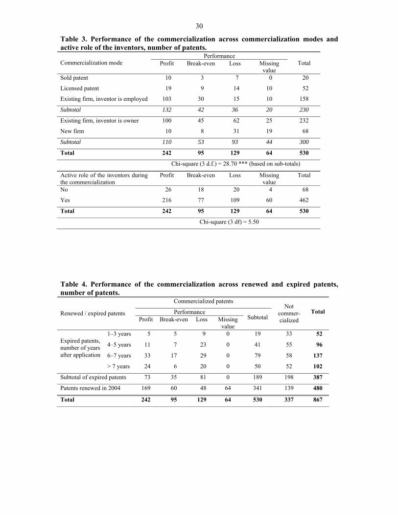
30

Table 3. Performance of the commercialization across commercialization modes and active role of the inventors, number of patents.

Performance Commercialization mode Profit Break-even Loss Missing

value

Total

Sold patent 10 3 7 0 20

Licensed patent 19 9 14 10 52

Existing firm, inventor is employed 103 30 15 10 158

Subtotal 132 42 36 20 230

Existing firm, inventor is owner 100 45 62 25 232

New firm 10 8 31 19 68

Subtotal 110 53 93 44 300

Total 242 95 129 64 530

Chi-square (3 d.f.) = 28.70 *** (based on sub-totals)

Active role of the inventors during the commercialization

Profit Break-even Loss Missing value

Total

No 26 18 20 4 68

Yes 216 77 109 60 462

Total 242 95 129 64 530

Chi-square (3 df) = 5.50

Table 4. Performance of the commercialization across renewed and expired patents, number of patents.

Commercialized patents

Performance Renewed / expired patents Profit Break-even Loss Missing

value Subtotal

Not commer-cialized

Total

1–3 years 5 5 9 0 19 33 52

4–5 years 11 7 23 0 41 55 96

6–7 years 33 17 29 0 79 58 137

Expired patents, number of years after application

> 7 years 24 6 20 0 50 52 102

Subtotal of expired patents 73 35 81 0 189 198 387

Patents renewed in 2004 169 60 48 64 341 139 480

Total 242 95 129 64 530 337 867

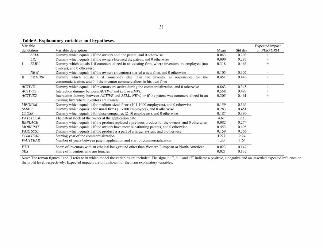
31

Table 5. Explanatory variables and hypotheses. Variable denotation

Variable description

Mean

Std dev.

Expected impact on PERFORM

I

SELL LIC EMPL NEW

Dummy which equals 1 if the owners sold the patent, and 0 otherwise Dummy which equals 1 if the owners licensed the patent, and 0 otherwise Dummy which equals 1 if commercialized in an existing firm, where inventors are employed (not owners), and 0 otherwise Dummy which equals 1 if the owners (inventors) started a new firm, and 0 otherwise

0.043 0.090 0.318

0.105

0.203 0.287 0.466

0.307

+ + +

– II EXTERN

Dummy which equals 1 if somebody else than the inventor is responsible for the commercialization, and 0 if the inventor commercializes in his own firm

0.451

0.440 +

ACTIVE ACTIVE1 ACTIVE2

Dummy which equals 1 if inventors are active during the commercialization, and 0 otherwise Interaction dummy between ACTIVE and LIC or EMPL Interaction dummy between ACTIVE and SELL, NEW, or if the patent was commercialized in an existing firm where inventors are owners

0.863 0.558 0.305

0.345 0.497 0.461

+ + +

MEDIUM SMALL CLOSE

Dummy which equals 1 for medium-sized firms (101-1000 employees), and 0 otherwise Dummy which equals 1 for small firms (11-100 employees), and 0 otherwise Dummy which equals 1 for close companies (2-10 employees), and 0 otherwise

0.159 0.283 0.187

0.366 0.451 0.390

PATSTOCK REPLACE MOREPAT PARTSYST

The patent stock of the owner at the application date Dummy which equals 1 if the product replaced a previous product for the owners, and 0 otherwise Dummy which equals 1 if the owners have more substituting patents, and 0 otherwise Dummy which equals 1 if the product is a part of a larger system, and 0 otherwise

4.61 0.082 0.453 0.159

12.13 0.274 0.498 0.366

COMYEAR WAITYEAR

Starting year of the commercialization Number of years between patent application and start of commercialization

1997 1.33

2.24 1.64

ETH SEX

Share of inventors with an ethnical background other than Western European or North-American Share of inventors who are females

0.023 0.021

0.147 0.132

Note: The roman figures I and II refer to in which model the variables are included. The signs “+.”, “–” and “?” indicate a positive, a negative and an unsettled expected influence on the profit level, respectively. Expected impacts are only shown for the main explanatory variables.

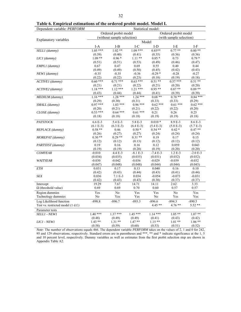
32

Table 6. Empirical estimations of the ordered probit model. Model I. Dependent variable: PERFORM Statistical model:

Ordered probit model (without sample selection)

Ordered probit model (with sample selection)

Model Explanatory variables

I-A I-B I-C I-D I-E I-F SELL1 (dummy) LIC1 (dummy) EMPL1 (dummy) NEW1 (dummy)

1.05 *** (0.39)

1.09 ** (0.51) 0.67

(0.49) -0.35 (0.22)

1.02 ** (0.40) 0.96 * (0.51) 0.47

(0.49) -0.35 (0.22)

1.09 *** (0.41)

1.11 ** (0.53) 0.69

(0.50) -0.36 (0.23)

0.85** (0.35) 0.85 * (0.49) 0.55

(0.45) -0.29 * (0.18)

0.77 ** (0.36) 0.73

(0.46) 0.40

(0.42) -0.28 (0.19)

0.80 ** (0.36) 0.79 * (0.47) 0.44

(0.43) -0.27 (0.18)

ACTIVE1 (dummy) ACTIVE2 (dummy)

0.60 *** (0.21)

1.18 *** (0.43)

0.71 *** (0.21)

1.12 *** (0.44)

0.63 *** (0.22)

1.21 *** (0.44)

0.51 ** (0.21)

0.95 ** (0.41)

0.57 *** (0.20)

0.87 ** (0.39)

0.51 ** (0.20)

0.89 ** (0.39)

MEDIUM (dummy) SMALL (dummy) CLOSE (dummy)

1.16 *** (0.29)

0.97 *** (0.20)

0.53 *** (0.18)

1.28 *** (0.30) 1.03 *** (0.21) 0.64 *** (0.18)

1.24 *** (0.31) 0.96 *** (0.21) 0.61 *** (0.18)

0.68 ** (0.33) 0.62 *** (0.22) 0.21 (0.19)

0.70 ** (0.33) 0.61 *** (0.22) 0.26 (0.19)

0.84 *** (0.29) 0.62 *** (0.20) 0.25 (0.18)

PATSTOCK REPLACE (dummy) MOREPAT (dummy) PARTSYST (dummy)

6.6 E-3 (6.1 E-3) 0.58 ** (0.26)

0.30 ** (0.12) 0.19

(0.19)

5.4 E-3 (6.3 E-3)

0.46 (0.27)

0.29 ** (0.12) 0.16

(0.19)

5.8 E-3 (6.4 E-3)

0.50 * (0.27)

0.31 ** (0.13) 0.16

(0.20)

0.010 * (5.4 E-3) 0.54 ** (0.24) 0.19

(0.12) 0.12

(0.19)

8.9 E-3 (5.8 E-3)

0.42 * (0.24) 0.17

(0.12) 0.059 (0.20)

8.6 E-3 (5.7 E-3) 0.47 ** (0.24) 0.15

(0.12) 0.043 (0.20)

COMYEAR WAITYEAR

-0.010 (0.034) -0.030 (0.047)

4.4 E-3 (0.035) -0.042 (0.048)

-8.1 E-3 (0.035) -0.036 (0.048)

-7.4 E-3 (0.031) -0.029 (0.044)

1.2 E-3 (0.032) -0.039 (0.044)

-2.0 E-3 (0.032) -0.032 (0.043)

ETH SEX

0.031 (0.42) 0.036 (0.42)

0.17 (0.43)

7.1 E-3 (0.43)

0.13 (0.44) 0.034 (0.43)

0.040 (0.43) -0.054 (0.38)

0.16 (0.41)

-0.073 (0.37)

0.10 (0.44) -0.031 (0.37)

Intercept Ω (threshold value)

19.29 0.69

7.67 0.69

14.71 0.70

14.11 0.60

2.62 0.57

3.33 0.57

Region dummies Technology dummies

Yes No

No Yes

Yes Yes

Yes No

No Yes

Yes Yes

Log Likelihood function Test vs. restricted model (1 d.f.)

-898.8 -896.7 -893.3 -896.6 4.45 **

-894.3 4.76 **

-890.5 5.52 **

Parameter tests SELL1 - NEW1 LIC1 - NEW1

1.40 *** (0.48)

1.43 ** (0.58)

1.37 *** (0.49)

1.31 ** (0.59)

1.45 *** (0.49)

1.47 ** (0.60)

1.14 *** (0.41)

1.15 ** (0.53)

1.05 ** (0.43)

1.01 ** (0.51)

1.07 ** (0.42)

1.06 ** (0.52)

Note: The number of observations equals 466. The dependent variable PERFORM takes on the values of 2, 1 and 0 for 242, 95 and 129 observations, respectively. Standard errors are in parentheses and ***, ** and * indicate significance at the 1, 5 and 10 percent level, respectively. Dummy variables as well as estimates from the first probit selection step are shown in Appendix Table A2.

33

Table 7. Empirical estimations of the ordered probit model. Model II. Dependent variable: PERFORM Statistical model:

Ordered probit model (without sample selection)

Ordered probit model (with sample selection)

Model Explanatory variables

II-A II-B II-C II-D II-E II-F EXTERN (dummy) 1.05 ***

(0.37) 0.97 ***

(0.37) 1.09 ***

(0.38) 0.83 ** (0.33)

0.65 ** (0.28)

0.70 ** (0.31)

ACTIVE1 (dummy) ACTIVE2 (dummy)

0.53 *** (0.19)

1.25 *** (0.38)

0.61 *** (0.20)

1.24 *** (0.39)

0.56 *** (0.20)

1.29 *** (0.39)

0.45 ** (0.17)

0.98 *** (0.35)

0.46 *** (0.14)

0.82 *** (0.29)

0.43 *** (0.16)

0.86 *** (0.32)

MEDIUM (dummy) SMALL (dummy) CLOSE (dummy)

0.98 *** (0.24)

0.91 *** (0.16)

0.56 *** (0.16)

1.03 *** (0.24) 0.94 *** (0.17) 0.66 *** (0.16)

1.06 *** (0.25) 0.90 *** (0.17) 0.65 *** (0.17)

0.50 * (0.28) 0.55 *** (0.19) 0.22 (0.17)

0.26 (0.22) 0.37 *** (0.15) 0.11 (0.14)

0.53 ** (0.22) 0.48 *** (0.15) 0.19 (0.15)

PATSTOCK REPLACE (dummy) MOREPAT (dummy) PARTSYST (dummy)

5.8 E-3 (5.9 E-3) 0.54 ** (0.27)

0.28 ** (0.12) 0.23

(0.18)

4.5 E-3 (6.1 E-3)

0.42 (0.27)

0.26 ** (0.12) 0.21

(0.19)

5.3 E-3 (6.3 E-3)

0.47 * (0.27)

0.28 ** (0.13) 0.20

(0.19)

9.8 E-3 * (5.1 E-3) 0.51 ** (0.24) 0.16

(0.12) 0.15

(0.18)

0.011 * (4.8 E-3)

0.42 * (0.25) 0.066 (0.10) 0.086 (0.19)

9.3 E-3 * (5.1 E-3)

0.45 * (0.24) 0.11

(0.11) 0.069 (0.18)

COMYEAR WAITYEAR

-0.013 (0.034) -0.023 (0.047)

-6.1 E-3 (0.035) -0.033 (0.047)

-0.011 (0.035) -0.029 (0.048)

-9.1 E-3 (0.030) -0.023 (0.043)

-2.6 E-3 (0.028) -0.028 (0.038)

-2.1 E-3 (0.029) -0.024 (0.040)

ETH SEX

0.072 (0.42) -0.042 (0.42)

0.24 (0.43) -0.096 (0.42)

0.15 (0.43) -0.047 (0.43)

0.055 (0.40) -0.12 (0.37)

0.011 (0.37)

-0.16 (0.31)

0.54 (0.40) -0.097 (0.34)

Intercept Ω (threshold value)

24.01 0.68

11.00 0.68

19.41 0.70

17.44 0.58

5.20 0.46

3.77 0.51

Region dummies Technology dummies

Yes No

No Yes

Yes Yes

Yes No

No Yes

Yes Yes

Log Likelihood function Test vs. restricted model (1 d.f.)

-901.9 -900.6 -896.3 -899.3 5.33 **

-897.2 6.73 ***

-893.6 5.48 **

Note: The number of observations equals 803. The dependent variable PERFORM takes on the values of 2, 1 and 0 for 242, 95 and 129 observations, respectively. Standard errors are in parentheses and ***, ** and * indicate significance at the 1, 5 and 10 percent level, respectively. Dummy variables as well as estimates from the first probit selection step are shown in Appendix Table A3.

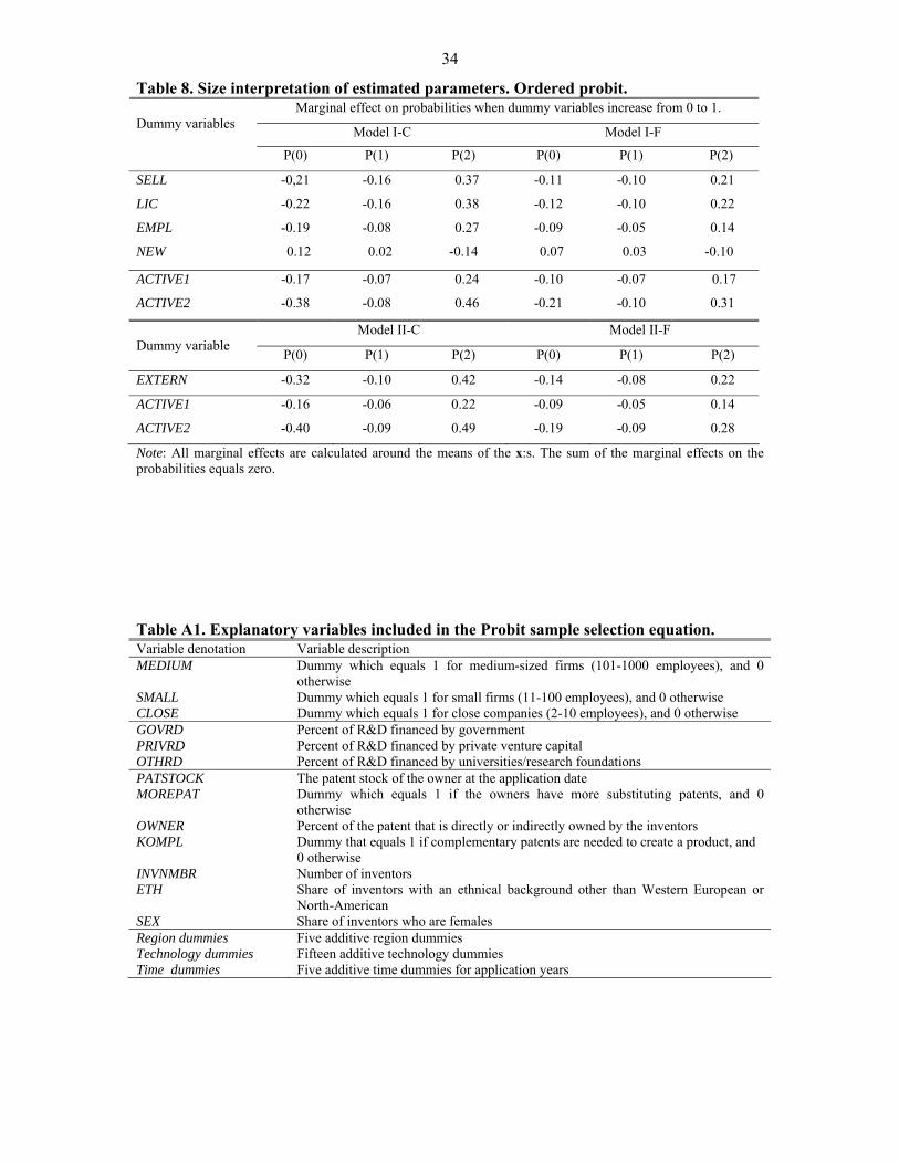
34

Table 8. Size interpretation of estimated parameters. Ordered probit. Marginal effect on probabilities when dummy variables increase from 0 to 1.

Model I-C Model I-F

Dummy variables

P(0) P(1) P(2) P(0) P(1) P(2)

SELL

LIC

EMPL

NEW

-0,21

-0.22

-0.19

0.12

-0.16

-0.16

-0.08

0.02

0.37

0.38

0.27

-0.14

-0.11

-0.12

-0.09

0.07

-0.10

-0.10

-0.05

0.03

0.21

0.22

0.14

-0.10

ACTIVE1

ACTIVE2

-0.17

-0.38

-0.07

-0.08

0.24

0.46

-0.10

-0.21

-0.07

-0.10

0.17

0.31

Model II-C Model II-F Dummy variable

P(0) P(1) P(2) P(0) P(1) P(2)

EXTERN -0.32 -0.10 0.42 -0.14 -0.08 0.22

ACTIVE1

ACTIVE2

-0.16

-0.40

-0.06

-0.09

0.22

0.49

-0.09

-0.19

-0.05

-0.09

0.14

0.28

Note: All marginal effects are calculated around the means of the x:s. The sum of the marginal effects on the probabilities equals zero. Table A1. Explanatory variables included in the Probit sample selection equation. Variable denotation Variable description MEDIUM SMALL CLOSE

Dummy which equals 1 for medium-sized firms (101-1000 employees), and 0 otherwise Dummy which equals 1 for small firms (11-100 employees), and 0 otherwise Dummy which equals 1 for close companies (2-10 employees), and 0 otherwise

GOVRD PRIVRD OTHRD

Percent of R&D financed by government Percent of R&D financed by private venture capital Percent of R&D financed by universities/research foundations

PATSTOCK MOREPAT OWNER KOMPL INVNMBR ETH SEX

The patent stock of the owner at the application date Dummy which equals 1 if the owners have more substituting patents, and 0 otherwise Percent of the patent that is directly or indirectly owned by the inventors Dummy that equals 1 if complementary patents are needed to create a product, and 0 otherwise Number of inventors Share of inventors with an ethnical background other than Western European or North-American Share of inventors who are females

Region dummies Technology dummies Time dummies

Five additive region dummies Fifteen additive technology dummies Five additive time dummies for application years

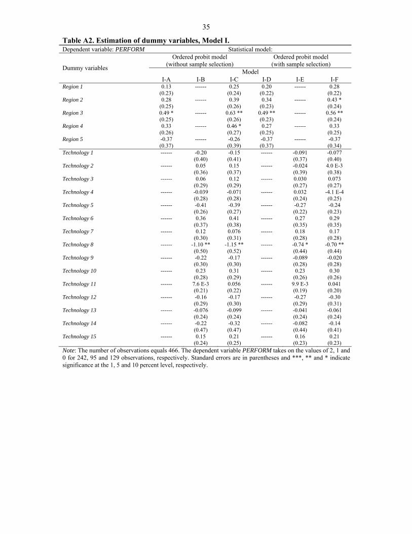
35

Table A2. Estimation of dummy variables, Model I. Dependent variable: PERFORM Statistical model:

Ordered probit model (without sample selection)

Ordered probit model (with sample selection)

Model Dummy variables

I-A I-B I-C I-D I-E I-F Region 1 Region 2 Region 3 Region 4 Region 5

0.13 (0.23) 0.28

(0.25) 0.49 * (0.25) 0.33

(0.26) -0.37 (0.37)

------

------

------

------

------

0.25 (0.24) 0.39

(0.26) 0.63 ** (0.26) 0.46 * (0.27) -0.26 (0.39)

0.20 (0.22) 0.34

(0.23) 0.49 ** (0.23) 0.27

(0.25) -0.37 (0.37)

------

------

------

------

------

0.28 (0.22) 0.43 * (0.24)

0.56 ** (0.24) 0.33

(0.25) -0.37 (0.34)

Technology 1 Technology 2 Technology 3 Technology 4 Technology 5 Technology 6 Technology 7 Technology 8 Technology 9 Technology 10 Technology 11 Technology 12 Technology 13 Technology 14 Technology 15

------

------

------

------

------

------

------

------

------

------

------

------

------

------

------

-0.20 (0.40) 0.05

(0.36) 0.06

(0.29) -0.039 (0.28) -0.41 (0.26) 0.36

(0.37) 0.12

(0.30) -1.10 ** (0.50) -0.22 (0.30) 0.23

(0.28) 7.6 E-3 (0.21) -0.16 (0.29) -0.076 (0.24) -0.22 (0.47) 0.15

(0.24)

-0.15 (0.41) 0.15

(0.37) 0.12

(0.29) -0.071 (0.28) -0.39 (0.27) 0.41

(0.38) 0.076 (0.31)

-1.15 ** (0.52) -0.17 (0.30) 0.31

(0.29) 0.056 (0.22) -0.17 (0.30) -0.099 (0.24) -0.32 (0.47) 0.21

(0.25)

------

------

------

------

------

------

------

------

------

------

------

------

------

------

------

-0.091 (0.37) -0.024 (0.39) 0.030 (0.27) 0.032 (0.24) -0.27 (0.22) 0.27

(0.35) 0.18

(0.28) -0.74 * (0.44) -0.089 (0.28) 0.23

(0.26) 9.9 E-3 (0.19) -0.27 (0.29) -0.041 (0.24) -0.082 (0.44) 0.16

(0.23)

-0.077 (0.40)

4.0 E-3 (0.38) 0.073 (0.27)

-4.1 E-4 (0.25) -0.24 (0.23) 0.29

(0.35) 0.17

(0.28) -0.70 ** (0.44) -0.020 (0.28) 0.30

(0.26) 0.041 (0.20) -0.30 (0.31) -0.061 (0.24) -0.14 (0.41) 0.21

(0.23) Note: The number of observations equals 466. The dependent variable PERFORM takes on the values of 2, 1 and 0 for 242, 95 and 129 observations, respectively. Standard errors are in parentheses and ***, ** and * indicate significance at the 1, 5 and 10 percent level, respectively.

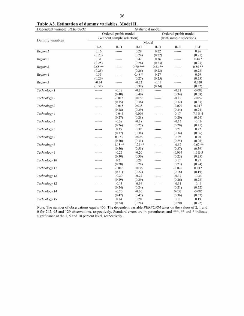
36

Table A3. Estimation of dummy variables, Model II. Dependent variable: PERFORM Statistical model:

Ordered probit model (without sample selection)

Ordered probit model (with sample selection)

Model Dummy variables

II-A II-B II-C II-D II-E II-F Region 1 Region 2 Region 3 Region 4 Region 5

0.16 (0.23) 0.31

(0.25) 0.55 ** (0.25) 0.35

(0.26) -0.34 (0.37)

------

------

------

------

------

0.29 (0.24) 0.42

(0.26) 0.70 ***

(0.26) 0.48 * (0.27) -0.22 (0.39)

0.22 (0.22) 0.36

(0.23) 0.53 ** (0.23) 0.27

(0.25) -0.13 (0.34)

------

------

------

------

------

0.26 (0.21) 0.44 * (0.23)

0.55 ** (0.23) 0.29

(0.25) 0.020 (0.32)

Technology 1 Technology 2 Technology 3 Technology 4 Technology 5 Technology 6 Technology 7 Technology 8 Technology 9 Technology 10 Technology 11 Technology 12 Technology 13 Technology 14 Technology 15

------

------

------

------

------

------

------

------

------

------

------

------

------

------

------

-0.18 (0.40) -0.013 (0.35) -0.015 (0.28) -0.044 (0.27) -0.38 (0.26) 0.35

(0.37) 0.073 (0.30)

-1.15 ** (0.50) -0.25 (0.30) 0.21

(0.28) -0.016 (0.21) -0.20 (0.29) -0.13 (0.24) -0.20 (0.47) 0.14

(0.24)

-0.15 (0.40) 0.079 (0.36) 0.038 (0.29) -0.096 (0.28) -0.38 (0.27) 0.39

(0.38) 0.026 (0.31)

-1.22 ** (0.51) -0.20 (0.30) 0.28

(0.28) 0.036 (0.22) -0.22 (0.29) -0.16 (0.24) -0.30 (0.47) 0.20

(0.24)

------

------

------

------

------

------

------

------

------

------

------

------

------

------

------

-0.11 (0.34) -0.12 (0.32) -0.070 (0.24) 0.17

(0.20) -0.15 (0.20) 0.21

(0.34) 0.19

(0.25) -0.52 (0.37) -0.064 (0.23) 0.17

(0.23) -0.026 (0.18) -0.37 (0.26) -0.11 (0.21) 0.053 (0.36) 0.11

(0.20)

-0.082 (0.38) -0.052 (0.33) 0.017 (0.24)

7.6 E-4 (0.24) -0.16 (0.21) 0.22

(0.36) 0.20

(0.26) -0.62 ** (0.39)

1.6 E-3 (0.25) 0.27

(0.24) 0.012 (0.19) -0.34 (0.28) -0.11 (0.22) -0.087 (0.37) 0.19

(0.22) Note: The number of observations equals 466. The dependent variable PERFORM takes on the values of 2, 1 and 0 for 242, 95 and 129 observations, respectively. Standard errors are in parentheses and ***, ** and * indicate significance at the 1, 5 and 10 percent level, respectively.