The Intuition Behind Option Valuation: A Teaching Note

Thomas Grossman Haskayne School of Business

University of Calgary

Steve Powell Tuck School of Business

Dartmouth College

Kent L Womack Tuck School of Business

Dartmouth College

Ying Zhang Tuck School of Business

Dartmouth College

Version 2.0. Copyright, 2002. All rights reserved. This document will be updated as appropriate and new versions will be available at HTTP://MBA.TUCK.DARTMOUTH.EDU/PAGES/FACULTY/KENT.WOMACK/TEACHING.HTM . We encourage any readers with suggestions or corrections to inform us by emailing KENT.WOMACK@DARTMOUTH.EDU. We thank our colleagues Ken Baker and Joel Vanden for helpful comments.

TABLE OF CONTENTS

1 INTRODUCTION .......................................................................................1

2 OPTION TERMS.......................................................................................1

3 OPTION PRICING BASICS.........................................................................3

3.1 A BASIC PV PROBLEM ......................................................................................3 3.2 THE CASE OF FIVE INVESTORS .........................................................................3 3.3 IF STOCK PRICES ARE UNCERTAIN ...................................................................4

4 THE GEOMETRIC BROWNIAN MOTION MODEL FOR STOCK PRICES .........6 4.1 KEY POINTS OF THE MODEL .............................................................................6 4.2 A REALISTIC PRICE PATH..................................................................................6 4.3 GBM PRICE PATHS ............................................................................................7

5 PRICING AN OPTION USING THE GBM MODEL ........................................9 5.1 BUILDING A DAILY MODEL FOR STOCK PRICES ..............................................9 5.2 USING THE DAILY MODEL TO PRICE AN OPTION...........................................11 5.3 SENSITIVITY OF FAIR OPTION VALUE TO KEY INPUTS .................................13

6 INTUITION BEHIND THE BLACK-SCHOLES FORMULA..............................17

7 CONCLUSION.........................................................................................21

8 BIBLIOGRAPHY OF VALUABLE REFERENCES..........................................21

1

The Intuition Behind Option Valuation: A Teaching Note

1 Introduction

Option valuation is one of the most difficult topics in the basic finance course. It is intimidating as being too abstract and involving too much mathematics. The purpose of this paper is to introduce the essential ideas behind option valuation using an intuitive and visual approach. We focus on building uncertainty in stock prices and its impact on option value through simple examples and simulation. Nothing more than a basic understanding of probability distributions and present value is required to follow our approach. We will first define the terms used in option valuation using a simple example. Then we will introduce a widely used model that describes the distribution of future stock prices1. Then we will use simulation to visualize stock price paths and derive a value for an option. Then we will analyze the sensitivity of the option value to the numerical assumptions. Finally, we draw the connections between our approach and the well-known Black-Scholes formula for option value. Throughout the paper we develop concepts and ideas around the following European call option on a stock we assume pays no dividend. The intuition behind option valuation, however, can easily be extended to other types of financial options. Example for discussion: A stock is currently trading at $48. A European call option on this stock can be purchased or sold with an expiration date six months from today and a strike price of $50. What should be the fair value of this option?

2 Option Terms What is a financial option? It is simply the right to buy (in the case of a call option) or sell (in the case of a put option) an asset, but without the obligation to do so at a given price called the strike price. Many types of assets may be behind the option: stocks, bonds, foreign currencies, etc. In this paper we will discuss an option contract on a share of stock. Most of the time, options on stocks are priced per share, but are traded in lots of 100 shares called a contract.

1 In this paper, “future price” means “spot price in a future time”.

2

Two important concepts are essential to understanding options: the strike price and the expiration date. The strike price is the price at which the option owner may buy or sell the underlying stock. The action of buying or selling the stock given ownership of the option is known as exercising the option. In our example, if the owner of this call option decides to exercise the option, he or she may buy the stock by paying $50, no matter what the market price of the stock is. Of course, the option owner has no obligation to buy the stock but can simply let the option expire if it is not advantageous to buy the stock at $50. The expiration date is the date when the option contract expires. After that date, the seller (often called “writer”) of the option no longer has the obligation to sell (or, buy) the stock to the owner of the call (or, put) option contract. In our example, the option contract expires six months from today. There are mainly two types of options – European and American. A European option can be exercised only on the expiration date, while an American option can be exercised at any time after it has been purchased up to the date of expiration. In our example, the owner of the European call option can only buy the underlying stock, or let the option expire, at the expiration date, but not at any time earlier. The owner of this option would not want to exercise this call and buy the stock for the strike price of $50 if the stock is trading six months from now below $50. He or she would be better off buying the stock at the lower price in the market! However, as the owner of a call option, you would exercise the option if the stock price were, say, $60 in the market, because you as option owner can effectively buy at $50 rather than $60. In this case you could make a $10 gain by exercising the option and buying the stock at $50, then selling the stock in the market at the then-prevailing price of $60. An option contract is like a gamble on the future stock price. One may or may not be able to profit from this gamble, but one needs to value this option and decide today whether to take the bet. A put option is akin to a car insurance policy, in which you buy a policy today to protect yourself against uncertain liabilities in the future (e.g., if you have a wreck). Suppose now you have the choice to buy the European call option in our example. Would you buy it? It should depend on whether the price you would have to pay is a fair value! The fair value of an option may be different from the option’s actual market price. The fair value can be thought of as the amount a smart bookie would pay to take on a bet today on the price difference between the stock price and the strike price at expiration.

3

3 Option Pricing Basics

3.1 A basic PV problem Let’s start with the simplest situation. Suppose we know that the price of the stock in question in six months will be $60, what is the fair value (i.e. what should one pay?) for this European call option with a strike price of $50? If the stock sells for $60 in six months, we could exercise the option to buy the stock for $50 and then immediately sell it on the market for $60, for a profit of $10. In another words, the European call option has a value of $10 in six months. What is the fair value of this European call option today? We simply need to discount the option payoff in six months back to today. Therefore, the option valuation becomes a simple present value problem. Suppose the expected annual rate of return is 7%. If we use the expected rate of return as discount rate, we will come up with an option value, i.e., the present value (PV) of the option payoff at expiration:

$10/(1 + 0.07/2) = $9.66

3.2 The case of five investors Now let’s extend the example to include five different investors, who try to forecast the stock price of the underlying stock at the expiration date. They believe that the price of the stock would be $30, $40, $50, $60, and $71 at expiration, respectively. Assuming the five investors have the same expected annual rate of return, 7%, what is the value2 (i.e. what would they be willing to pay?) for this European call option? As described above, to determine the value we find the option payoff at expiration, and then discount this payoff back to today using the expected rate of return as discount rate. In this case, the option value is different from the perspectives of the five investors, because they anticipate different stock prices at expiration. Table 3.2 summarizes the option payoffs and the corresponding option values in the eyes of the 5 investors.

2 This value is not yet the fair arbitrage-free (Black-Scholes) value of the option.

4

Investor Stock Price at

Expiration Strike Price Option Payoff at

Expiration Option Value

ST X MAX (0,ST-X) PV (Option Payoff) # 1 71 50 21 20.29 # 2 60 50 10 9.66 # 3 50 50 0 0 # 4 40 50 0 0 # 5 30 50 0 0

Table 3.2

Note that when the stock price at expiration is less than or equal to the strike price of $50, one would not exercise the call option. In these cases, the option has no inherent value in six months, and hence should be worth nothing today. Therefore, investors #3, #4, and #5 would not pay anything for the call option with a strike price of $50, if they believe with certainty their six-month stock price forecasts of $50, $40, and $30. Here are some of the key ideas this example illustrates:

• A European call option pays off only when the stock price at the expiration date exceeds the strike price. • The option payoff in Table 3.2, MAX (0,ST-X), is called the intrinsic value at expiration. Intrinsic value is defined as the value an option would have if it were exercised immediately, so an option may have different intrinsic values at different points of time. For a call option, it is the maximum of zero and ST-X, where ST stands for the stock price at a point of time, T, and X is the strike price. We use “intrinsic value” in this paper to mean “intrinsic value at expiration,” because that is the only intrinsic value that matters for valuing a European option. • The option value is the present value of the option’s intrinsic value.

3.3 If stock prices are uncertain In the real world, seeing through a crystal ball to get a perfectly accurate future stock price is nearly impossible. The best we can hope for is to estimate a probability distribution of the stock price at expiration. The probability distribution is essentially a set of possible scenarios, each with its own probability of occurring. So, the probability distribution for the future stock price specifies the possible outcomes for the price and the probabilities of each outcome occurring. We will discuss later how to create a realistic probability distribution for stock prices. At this stage, we will (unrealistically) assume that we know the probability

5

distribution of the stock price at expiration. Let’s assume there is an equal chance (20%) that each of the five investors is correct in his or her forecast of the future stock price. The option intrinsic values and their corresponding present values for different price scenarios have been calculated in Table 3.3. In order to find the value of this European call, we should weigh these present values by their probabilities of occurring. The sum of the probability-weighted present values should be the option value. Again here we use the expected rate of return as the discount rate. Table 3.3 summarizes the calculation of the probability-weighted present values of option intrinsic values. Stock Price at

Expiration Strike Price

Intrinsic Value PV of Intrinsic Value

Prob. Prob.-weighted PV

ST X MAX (0,ST-X) Prob. x PV 71 50 21 20.29 20% 4.06 60 50 10 9.66 20% 1.93 50 50 0 0 20% 0 40 50 0 0 20% 0 30 50 0 0 20% 0

5.99

Option Value

Table 3.3

Note that the option value, $5.99, is the sum of the probability-weighted present values, i.e., 4.06 + 1.93 + 0 + 0 + 0. An alternative approach would be to take the average of the present values of the intrinsic values for different scenarios, i.e.,

$5.99 = 0.20 * (20.99+9.66+0+0+0) In this example, each of the outcomes for the stock price is assumed to be equally likely, so the intrinsic values receive the same weight in determining the option value. If we have good reason to believe that the chances for the five prices to occur at expiration are different, we would assign different probabilities to them, and then apply the same probability-weighted method to come up with an option value. Thus the option value is the sum of the probability-weighted present values of intrinsic value, i.e.

C = Σ {Prob(Se) * PV (max[0, Se-X])}, where C is the call option value, Se is the stock price at expiration, and X is the strike price.

6

4 The Geometric Brownian Motion Model for Stock Prices

4.1 Key points of the model As described previously, the stock price at expiration is the key to the value of a European option, but it is nearly impossible to predict stock prices exactly. The examples in the previous section demonstrated how we would determine an option value if we had realistic information about the stock price at expiration. What we need at this point is a model that can describe a stock’s price in the future, given the current stock price and other information about the stock itself. We should not expect the model to tell us the future stock price exactly, but instead give us a probability distribution for the future price. One such model that will provide a future stock price probability distribution is Geometric Brownian Motion (GBM). The essence of GBM is that future returns on a stock are normally distributed with a mean upward drift, and a standard deviation that can be estimated using historical data. This statement about stock returns being normally distributed leads to the conclusion that the future price of a stock is log-normally distributed. That is, the distribution of stock prices is asymmetric, with values above the mean more likely than values below the mean. We will now illustrate how the GBM generates realistic price paths.

4.2 A realistic price path Let’s take a look at a realistic price path. Many stock price chart looks like Figure 4.2.

Today Future

7

Figure 4.2 There are two noticeable features of this price path: trend and fluctuation. The trend is the overall movement in the price, which is upwards in the example above. The fluctuations in the price around this upward trend reflect the volatility in prices over time. The intensity of daily price fluctuations (or, jumps) determines the volatility of the stock. Volatility measures the uncertainty of the return realized on a stock. Statistically, it is the standard deviation of returns for a short period of time, since obviously, not all days’ returns are equal. Historical volatility measures are available for most stocks in the databases of financial information providers such as Bloomberg. Intuitively, any realistic model that describes stock price paths over a specific period of time t from today to a future time should look something like this:

St = S0 *growth factor, where S0 and St stand for the current and future stock prices, respectively, and the growth factor should take into account the above-mentioned overall trend (the upward shift) and volatility of the particular stock in question. We will see shortly that the GBM model does have this form.

4.3 GBM price paths

The GBM model states that future returns on a stock are normally distributed. The return on a stock can be defined as the logarithm of the ratio of successive prices, i.e. ln(St /S0). Students without extensive mathematical training need to accept this statement and keep going. If the return is normally distributed, then ln(St /S0) has an average value, µ, (the trend) and a spread measured by its standard deviation, σ. The mean is the expected rate of return on the stock, and the standard deviation is the volatility of the stock over the same period of time. Usually, we have data on the annual rate of return and volatility for stocks. But since we will want to model stock prices over shorter periods of time (e.g. daily), we will need to convert time units. If µ is the annual rate of return on the stock, and σ is the annualized volatility (standard deviation), then the mean and standard

8

deviation for a period (a fraction of a year) t should be µt and σ√t, respectively3. Since returns are given by the normal distribution, we can now express the GBM model in the form:

ln(St /S0) ≈ N(µt, σ√t), where N(µt, σ√t) refers to a normal distribution with mean µt and standard deviation σ√t.

We can rearrange this equation by raising each side to the power e, and remembering that e(ln(x)) = x. The result is:

St = S0 * e N(µt, σ√t)

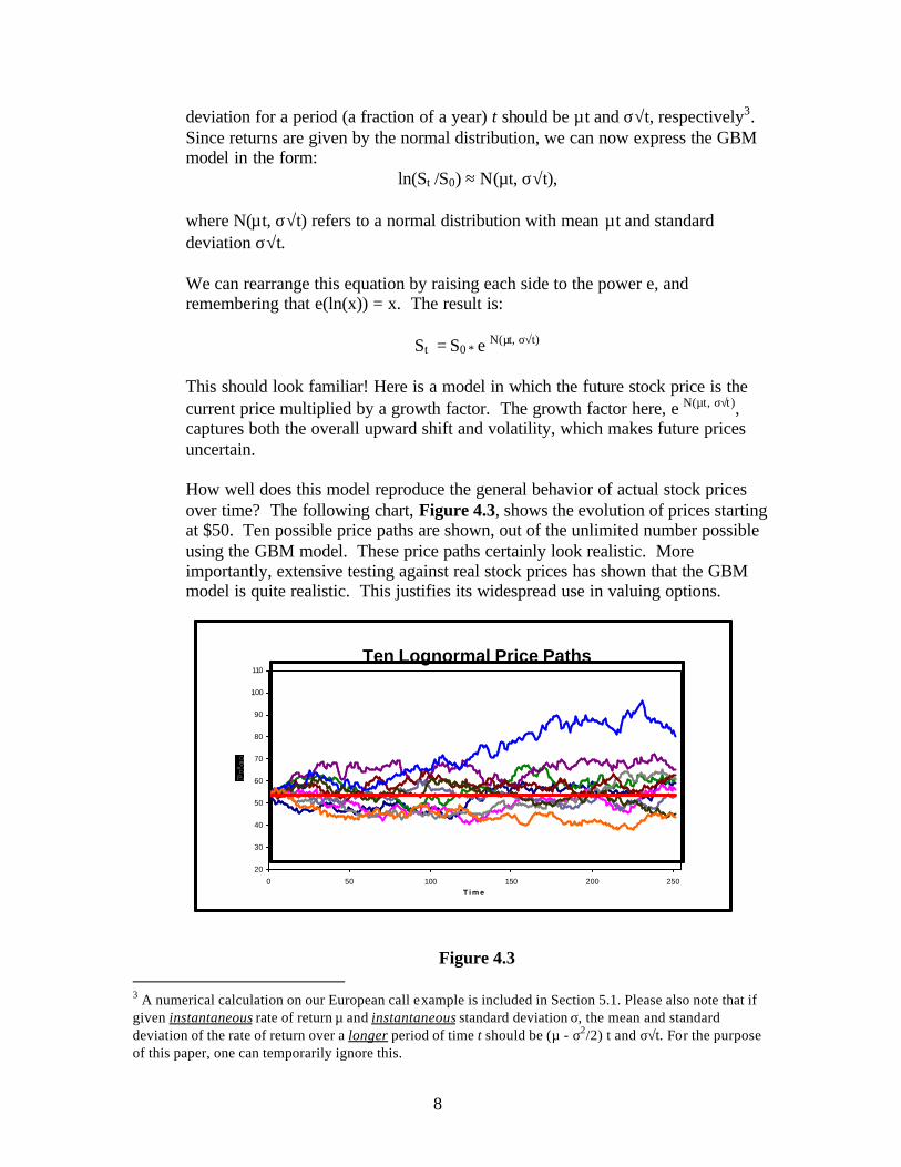
This should look familiar! Here is a model in which the future stock price is the current price multiplied by a growth factor. The growth factor here, e N(µt, σ√t ), captures both the overall upward shift and volatility, which makes future prices uncertain. How well does this model reproduce the general behavior of actual stock prices over time? The following chart, Figure 4.3, shows the evolution of prices starting at $50. Ten possible price paths are shown, out of the unlimited number possible using the GBM model. These price paths certainly look realistic. More importantly, extensive testing against real stock prices has shown that the GBM model is quite realistic. This justifies its widespread use in valuing options.

Ten Lognormal Price Paths

20

30

40

50

60

70

80

90

100

110

0 50 100 150 200 250Time

Figure 4.3 3 A numerical calculation on our European call example is included in Section 5.1. Please also note that if given instantaneous rate of return µ and instantaneous standard deviation σ, the mean and standard deviation of the rate of return over a longer period of time t should be (µ - σ2/2) t and σ√t. For the purpose of this paper, one can temporarily ignore this.

9

5 Pricing an Option using the GBM Model

5.1 Building a daily model for stock prices

The GBM model specifies for us the random process behind the evolution of stock prices over time. If we know the current price, as well as the mean and standard deviation of the price over time, we can project the actual price forward simply by taking random samples from the normal distribution that determines the growth factor. We will now do that using Crystal Ball, an add- in for Excel that automates the process of random sampling. For our example, we will suppose that the expected annual rate of return of the underlying stock is µ (=7%), and the annualized volatility is σ (=30%). We will again use the expected rate of return as the discount rate. Our first step is to convert the annual rate of return and annualized volatility into daily equivalents (assuming 250 trading days per year):

µt = 7% * (1/250) = 0.028% σ√t = 30% * √(1/250) = 1.897%

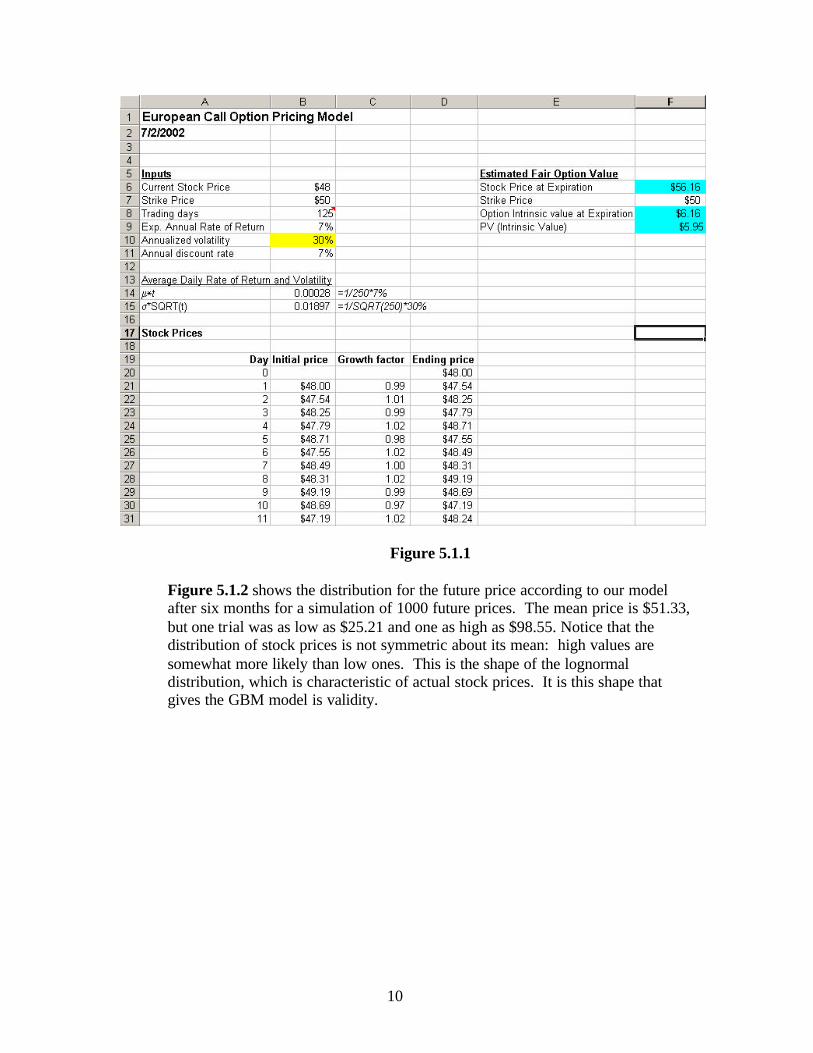
Therefore, the daily growth factor, e N(µt, σ√t) , becomes e N(0.028%, 1.897%) In the spreadsheet shown below (see Figure 5.1.1), we have entered the numerical assumptions and calculated the daily mean and volatility. The model for stock prices in Figure 5.1.1 starts in row 20. We use four columns. The first column records the trading days from 1 to 125 (six months). The second column records the stock price at the beginning of the day, which is the stock price at the end of the previous day from the fourth column. The third column contains the random growth factor. The fourth column calculates the stock price at the end of the day by multiplying the price at the beginning of the day by that day’s growth factor. To calculate the random growth factors each day we use a special function from Crystal Ball: CB.Normal(mean, standard deviation). This function calculates a random sample from the given normal distribution for each of the days of our simulation. Every time we recalculate the spreadsheet we get a new set of samples for the growth factors for the 125 days, and thereby a new price path. If we repeat this sampling procedure many times, we can develop a probability model for the stock price at expiration, six months away.

10

Figure 5.1.1 Figure 5.1.2 shows the distribution for the future price according to our model after six months for a simulation of 1000 future prices. The mean price is $51.33, but one trial was as low as $25.21 and one as high as $98.55. Notice that the distribution of stock prices is not symmetric about its mean: high values are somewhat more likely than low ones. This is the shape of the lognormal distribution, which is characteristic of actual stock prices. It is this shape that gives the GBM model is validity.

11

Figure 5.1.2 In Figure 5.1.3 we have highlighted those outcomes in which the stock price after six months is at least $50, the strike price on our option. We can see (“Certainty”) that the price exceeds the strike price about 53% of the time; thus we can expect a buyer to exercise the option about that often.

Figure 5.1.3

5.2 Using the daily model to price an option

12

Now let’s add a module to the existing daily model to calculate the intrinsic value of the option and its present value. The mathematical mechanism is no different from the intrinsic value and present value calculations shown in Section 3. The option value is calculated in four steps, starting in cell F6 in the spreadsheet shown in Figure 5.1.1. First, we record the stock price on day 125. Second, we enter the strike price. Third, we calculate the intrinsic value at the expiration date using the formula

Max(0, Stock price at expiration – Strike price). Finally, we take the present value of the intrinsic value at the given interest rate. In the example shown in Figure 5.1.1, the stock price at expiration is $56.16, the strike price is $50, the intrinsic value is $6.16, and the present value is $5.95. When we take 1000 random samples for the growth factors, Crystal Ball will generate 1000 price paths and 1000 corresponding stock prices at expiration, which finally lead to 1000 present values of intrinsic values. Since each of these present values is equally likely, Crystal Ball simply averages all 1000 to determine our estimate of the value of this option. Please note that 1000 samples are only sufficient to give a very rough estimate of the option value. An estimate accurate to +/- $0.05 would take 50,000 samples or more.4 In Figure 5.2 we show the distribution of intrinsic values for this option. Notice that the intrinsic value is $0 about 47% of the time. As we saw above in Figure 5.1.3, the stock price only exceeds the strike price around 53% of the time, so in the other 47% of the outcomes we will let the option expire without exercising it and make nothing. The average intrinsic value is $4.94. This would be the value of the option, except that it is delayed six months. When discounted, this average intrinsic value is $4.77. This, finally, is a realistic estimate of the value of the option.

4 For additional insight on this issue, see Investment Science by David G. Luenberger, p. 364.

13

Figure 5.2

We simplified the calculation for the purpose of this article, by applying a universal discount rate, i.e., the expected rate of return on the underlying stock, to all the intrinsic values associated to different price paths. Options are generally riskier than stocks, so one would require higher return for owning options than he or she does for owning the underlying stocks. Moreover, if trying to determine the fair arbitrage-free option value using our spreadsheet approach, one should use different, and price-path dependent, rates to discount intrinsic values back to today, and then calculate the fair option value by summing up all the probability-weighted present values. (When we calculate arbitrage-free Black Scholes values in Section 6, this problem will disappear.)

5.3 Sensitivity of fair option value to key inputs

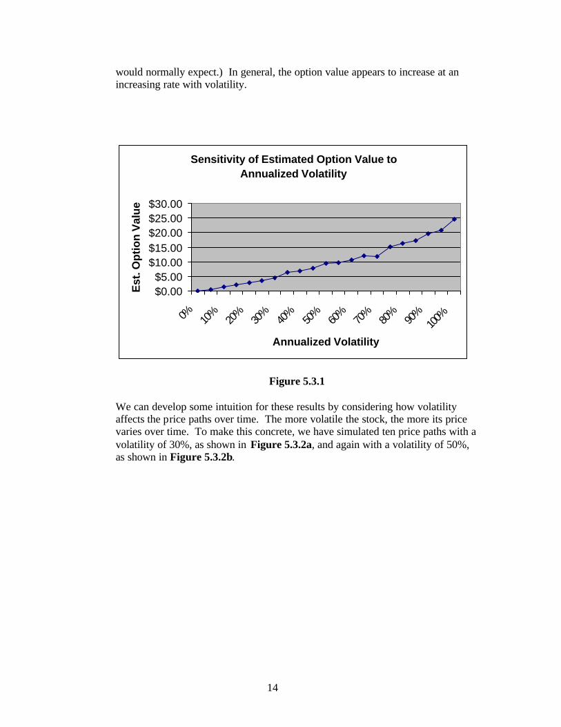
Now that we have determined a value for the option, it is interesting to consider how sensitive that value is to the inputs to the model. Two critical inputs are the volatility of the stock and the time to the expiration date. To test your intuition, and before reading on, try to formulate a qualitative guess as to how the value of the option will change if we were to change either one of these inputs. Volatility To test the sensitivity of option value to the volatility of the underlying stock we ran a set of simulations of our model, varying the volatility from 0 to 100%. The results are shown in Figure 5.3.1. We can see that the option has essentially no value when the volatility is low, but could be worth as much as $25 for extremely high volatilities. (Of course, an annual volatility of 100% is far beyond what we

14

would normally expect.) In general, the option value appears to increase at an increasing rate with volatility.

Sensitivity of Estimated Option Value to Annualized Volatility

$0.00$5.00

$10.00$15.00$20.00$25.00$30.00

0% 10%

20%

30%

40%

50%

60%

70%

80%

90%

100%

Annualized Volatility

Est

. Op

tio

n V

alu

e

Figure 5.3.1

We can develop some intuition for these results by considering how volatility affects the price paths over time. The more volatile the stock, the more its price varies over time. To make this concrete, we have simulated ten price paths with a volatility of 30%, as shown in Figure 5.3.2a, and again with a volatility of 50%, as shown in Figure 5.3.2b.

15

Ten Lognormal Price Paths

2030405060708090

100110

0 50 100 150 200 250Time

Volatility: 30%--narrow spread

Figure 5.3.2a

Ten Lognormal Price Paths

2030405060708090

100110

0 50 100 150 200 250Time

Volatility: 50%--wider spread

Figure 5.3.2b

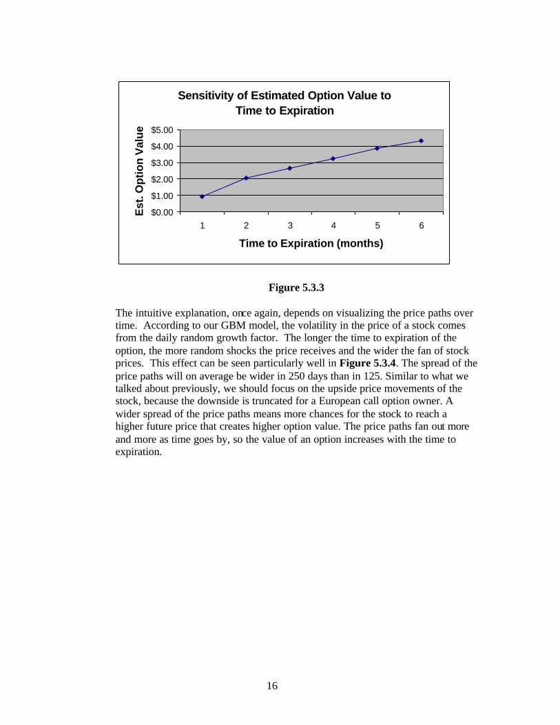
These figures illustrate that as the volatility increases, the price paths fan out more and more. With higher volatility, high price paths are more likely but so are low price paths. But for an owner of a European call option, as we have seen, it is high price paths that create option value. Higher price paths create higher option intrinsic values at expiration. Low price paths that lead to stock prices that are lower than strike price at expiration, on the other hand, simply give the same intrinsic value: zero. Thus as the volatility of the stock increases, the option intrinsic values on high price paths increase while those on low price paths do not change. This makes the option more valuable. Time to expiration To test the sensitivity of option value to the time to expiration, we ran another set of simulations, varying the expiration date from one to six months. The results are shown in Figure 5.3.3. A one-month option on our stock is worth less than $1, while a six-month option is worth more than $4.

Wider spread! (with volatility 50% rather than 30%)

16

Sensitivity of Estimated Option Value to Time to Expiration

$0.00

$1.00

$2.00

$3.00

$4.00

$5.00

1 2 3 4 5 6

Time to Expiration (months)

Est

. Op

tio

n V

alu

e

Figure 5.3.3 The intuitive explanation, once again, depends on visualizing the price paths over time. According to our GBM model, the volatility in the price of a stock comes from the daily random growth factor. The longer the time to expiration of the option, the more random shocks the price receives and the wider the fan of stock prices. This effect can be seen particularly well in Figure 5.3.4. The spread of the price paths will on average be wider in 250 days than in 125. Similar to what we talked about previously, we should focus on the upside price movements of the stock, because the downside is truncated for a European call option owner. A wider spread of the price paths means more chances for the stock to reach a higher future price that creates higher option value. The price paths fan out more and more as time goes by, so the value of an option increases with the time to expiration.

17

Ten Lognormal Price Paths

20

30

40

50

60

70

80

90

100

110

0 50 100 150 200 250Time

Pri

ce

Figure 5.3.4

6 Intuition behind the Black-Scholes Formula

We have now derived an estimated value of a European call option from simulating the underlying stock’s price paths and then calculating the probability-weighted present value of the option’s intrinsic value. Recall the inputs for option pricing, which include the price of the underlying stock, the volatility of the stock, the strike price, expiration date, and the expected rate of return of the stock. (Dividends paid before expiration date matter also, but we are assuming them away for our example. If dividends are paid, their present value will decrease the call option value, because they decrease the future stock price.) These above-mentioned parameters are also the inputs for the Black-Scholes options pricing formula for European call (and put) options5. Black-Scholes formula, however, values an option from the perspective of a trader who needs to hedge his short position in an option (meaning the trader who sells an option). The Black-Scholes value is the cost of that hedge. There are several important assumptions underlying Black-Scholes. If we apply these assumptions to our model as shown above, and run enough trials for the simulation, the derived estimated option value should be close to the Black-Scholes value. In the following paragraphs, we will first present the formula and then provide a brief and simple explanation. The reader should find in this process that the intuition that we have built using simulation remains valid for Black-Scholes.

5 In Black-Scholes formula, the risk-free rate of interest is used as expected rate of return.

18

The Black-Scholes formula for pricing a European call option on non-dividend-paying stocks is 6

C = SN(d1) – Xe-rT N(d2) where d1 = [ln(S/X) + (r + σ2/2)T] / σ√T d2 = [ln(S/X) + (r - σ2/2)T] / σ√T = d1 - σ√T

The variables in the formula are C: the fair (Black-Scholes) European call option value today S: the current price of the underlying stock X: the strike price r: the risk-free interest rate T: the time to expiration σ: the volatility of the stock We will build intuition about the normal distribution terms, N(d1) and N(d2), later. Suppose you want to profit (or, at a minimum, break even) from selling a European call option to another person, but do not have that stock in inventory. Is there any risk to you as a seller of the option? Of course there is. If the future stock price is greater than the strike price i.e., if the option finishes in the money, you will have to buy stock in the market and deliver it to the purchaser of the option for the strike price. The value you will owe is the difference between the then-prevailing stock price and the strike price you have promised to let the purchaser of the option pay for the share of stock. To hedge your sale of the option, you want to have some amount of a long position (you buy and hold) in the underlying stock to cover the risk of your short exposure in the call option if the stock price goes up. However, you do not want to buy and hold the stock position using your own money. So, you should borrow money, i.e. to short sell a bond, to finance the long position in the stock. Now take a look at your “balance sheet” of this “long-stock, short-bond” portfolio. You have the stock as your asset and the bond as your liability. You also have another liability outside this portfolio – it is the value of the option that has been sold. If the net value of the portfolio remains equal to the liability of the option contract sold, your risk will be hedged.

6 Here we focus on the formula for a European call option. The intuition for a European put option is similar.

19

You as an options “bookie” will need to adjust the portfolio at different points of time, by either selling stock to pay down some of the bond, or borrowing more money to buy stock, to make sure that at any point of time the net value of your “long-stock, short-bond” portfolio is equal to the value of the option. Meanwhile, ignoring transaction costs, you will not need to inject any additional fund into this portfolio once it is set up. This is often referred to as a “self- financing, replicating hedging” strategy. Your hedging portfolio replicates the value of the European call option at every point of time, and so once we value the hedging portfolio, we will have valued the option. At expiration, the call option will finish either in the money, or out of the money. If it finishes in the money, the option owner will exercise the option and will want the shares of the underlying stock to be delivered at the strike price. The hedger will then have to deliver the shares, and pay off the bond that is outstanding. To cover these two liabilities, the above-mentioned “self- financing, replicating” portfolio should contain exactly the number of shares that are required by the owner of the option; meanwhile, the amount of money paid by the option owner (based on the strike price) to call in those shares should be exactly enough for the hedger to pay off the then-outstanding bond liability. For instance, if the option in question is only one share, the value of the bond in the hedging portfolio at expiration should be equal to the strike price. Similarly, if the option finishes out of the money (and the option purchaser will not exercise his option), the portfolio will contain no shares and zero amount of bond (you have paid off all the bond liability) at expiration7. Today what is in the hedging portfolio? The hedger sets up the portfolio by purchasing some shares of the underlying stock and shorting some amount of bond (B). The value of this hedging portfolio should equal to the fair value of the European call option today, which is the value in question for Black-Scholes. At this point, the puzzle becomes how many shares of stock to buy and how much bond value to sell, i.e., Fair value of a European call option = ? shares of the underlying stock - B How much bond should the hedger sell? We do know that B=X at expiration if the option finishes in the money, so we can discount X by the continuously compounded rate of risk-free return to get the amount we need to short today if we knew that the option would finish in the money. As explained earlier, due to uncertainty in stock prices, we are not sure of the option payoff at expiration, and so the best we can do is to factor in the probability that the option will finish in the money. This probability changes over time, and is given by a differential equation that takes into account the uncertainty embedded in stock paths.

7 For additional insights, see Option Pricing: Black -Scholes Made Easy by Jerry Marlow, p. 133-141.

20

How many shares of the underlying stock should the hedger buy? The number of shares in the hedging portfolio today, similarly, can also be calculated through a differential equation. Let’s get back to the Black-Scholes formula:

C = SN(d1) – Xe-rT N(d2) The left side (C for call) signifies the Black-Scholes European call option value (the present value of the fair value of the gamble, played many times, that the stock will be higher than the strike price at expiration). It should be equivalent to the cost of setting up a hedging portfolio on the right side of the equation, where the seller of the call option buys some amount of shares of stock at current price S, and goes short some amount of Bond that equals to X at expiration if the option finishes in the money. e-rT is the discount (present valuing) factor , and so the “mysterious” N(d1) and N(d2) must be the number of shares (usually referred to as ∆) of the stock to go long today, and the probability that the option will finish in the money respectively. Both N(d1) and N(d2) change as the underlying stock price and the time to expiration change. This is why one needs to adjust the hedging portfolio continuously. It is not the purpose of this article to exhaust all the details and assumptions of the Black-Scholes formula, but we do want briefly discuss two points by focusing on d2 that is given by the following equation.

d2 = [ln(S/X) + (r - σ2/2)T] / σ√T

First, we circle the familiar items that we have talked about previously in this article.

These are the mean and standard deviation of the return on the stock over a period of time T, given instantaneous rate of return and standard deviation. The rate of return used here is the risk-free rate of return, r.

As we can see, the assumption that is embedded in the calculation of the probability that the option will finish in the money for the Black-Scholes formula is that stock price follows the lognormal paths given by GBM. Secondly, the rate of return adopted by the Black-Scholes formula is the risk-free interest rate, not the expected rate of return on the underlying stock. Why? The best explanation is by Fisher Black himself:8

8 “How We Came up with the Option Formula”, Journal of Portfolio Management 15, Winter 1989, pp. 4-8.

21

“…the option value will change when the stock price changes by a small amount within a short time. Suppose that the option goes up about $0.50 when the stock goes up $1.00, and down $0.50 when the stock goes down $1.00. Then you can create a hedged position by going short two option contracts and long one round lot of stock. Such a position will be close to riskless. For small moves in the stock in the short run, your losses on one side will be mostly offset by gains on the other side… As the hedged position will be close to riskless, it should return an amount equal to the short-term interest rate on close-to-riskless securities. This one principle gives us the option formula.”

7 Conclusion

The challenge in option valuation mainly lies in estimating the uncertainty in the underlying stock’s future price paths. For European options, the valuation involves deriving realistic (log-normal) price paths that lead to realistic probability distributions of future stock prices at expiration; calculating option intrinsic values; discounting intrinsic values back to today using appropriate discount rates, and summing up the probability-weighted present values to get the fair option value. These intuitions also contribute to the understanding of the well-known Black-Scholes formula.

8 Bibliography of Valuable References Neil A. Chriss, Black-Scholes And Beyond: Option Pricing Models, 1997 Lawrence C. Galitz, Financial Engineering: tools and techniques to manage financial risk, 1995 Jerry Marlow, Option Pricing: Black-Scholes Made Easy, 2001 John C. Hull, Futures And Options Markets, 1998