ISSN 8755-6839

SCIENCE OF

TSUNAMI HAZARDS The International Journal of The Tsunami Society Volume 19 Number 3 Published Electronically 2001

SOME OPPORTUNITIES OF THE LANDSLIDE TSUNAMI HYPOTHESIS

Phillip Watts

Applied Fluid Engineering

Long Beach, California 90803, USA

126

A NON-LINEAR NUMERICAL MODEL FOR STRATIFIED TSUNAMI WAVES AND ITS APPLICATION

Monzur Alam lmteaz The University of Queensland

Brisbane, QLD 4072, Australia

Fumihiko lmamura

Tohoku University

Aoba, Sendai 980-8579, Japan

MODELING THE LA PALMA LANDSLIDE TSUNAMI

Charles L. Mader

Mader Consulting Co., Honolulu, HI, USA

BOOK REVIEW - The Big One - The Next California Earthquake

by George Pararadarayannis

copyright @I 2001

THE TSUNAMI SOCIETY P. 0. Box 37970,

Honolulu, HI 96817, USA

WWW.STHJOURNAL.ORG

150

160

OBJECTIVE: The Tsunami Society publishes this journal to increase and disseminate knowledge about tsunamis and their hazards.

DISCLAIMER: Although these articles have been technically reviewed by peers, The Tsunami Society is not responsible for the veracity of any state- ment , opinion or consequences.

EDITORIAL STAFF

Dr. Charles Mader, Editor

Mader Consulting Co. 1049 Kamehame Dr., Honolulu, HI. 96825-2860, USA

EDITORIAL BOARD

Zygmunt Kowalik, University of Alaska

T. S. Murty, Baird and Associates - Ottawa

Shigehisa Nakamura, Kyoto University

Yurii Shokin, Novosibirsk

Thomas Sokolowski, Alaska Tsunami Warning Center

Costas Synolakis, University of California

Professor Stefano Tinti, University of Bologna

Dr. Antonio Baptista, Oregon Graduate Institute of Science and Technology

Professor George Carrier, Harvard University

Mr. George Curtis, University of Hawaii - Hilo

Dr.

Dr.

Dr.

Dr.

Mr

Dr.

TSUNAMI SOCIETY OFFICERS

Dr. Tad Murty, President

Mr. Michael Blackford, Secretary

Dr. Barbara H. Keating, Treasurer

Submit manuscripts of articles, notes or letters to the Editor. If an article is accepted for publication the author(s) must submit a scan ready manuscript or a PDF file in the journal format. Issues of the journal are published electronically in PDF format. The journal issues for 2001 are available at

http://www.sthjournal.org. Tsunami Society members will be advised by e-mail when a new issue is

available and the address for access. There are no page charges or reprints for authors.

Permission to use figures, tables and brief excerpts from this journal in scientific and educational works is hereby granted provided that the source is acknowledged. Previous volumes of the journal are available in PDF format at http://epubs.lanl.gov/tsunami/ and on a CD-ROM from the Society.

ISSN 8755-6839

http://www.sthjournal.org and http://www.ccalmr.ogi.edu/STH

Published Electronically by The Tsunami Society in Honolulu, Hawaii, USA

Science of Tsunami Hazards Volume 19, pages 126-149 (2001)

SOME OPPORTUNITITES OF THE

LANDSLIDE TSUNAMI HYPOTHESIS

Phillip Watts

Applied Fluids Engineering

PMB No. 237, 5710 E. 7th Street

Long Beach, California 90803, USA

ABSTRACT

Tsunami sources are intimately linked to geological events. Earthquakes and landslidesare shown to be part of a continuum of complicated geological phenomena. Advancesin landslide tsunami research will remain coupled with marine geology research. Thelandslide tsunami hypothesis is shown to have originated in the scientific literature in theearly 1900s. Tsunami science has been slow to embrace the hypothesis in part because ofthe tremendous uncertainity that it introduces into tsunami gneration. The 1998 PapuaNew Guyinea event sparked much controbersy regarding the landslide tsunami hypothesisdespite a preponderance of the evidence in favor of one simple and consistent explanationof the tsunami source. Part of the difficulty was the unanticipated distinction betweenslide and slump tsunami sources. Significant controversies still exist over other aspects ofthe Papua New Guinea event. The landslide hypothesis will become widely acceepted oncedirect measurements of underwater landslide events are made. These measurements willlikely be integrated into a local tsunami warning system.

Science of Tsunami Hazards Volume 19, pages 126-149 (2001)

INTRODUCTION

For the sake of argument, let us define a tsunami as the water waves resulting from an

identifiable geological event, which may involve an earthquake, a landslide, volcanic activity,

a gas diapirism, etc. Further, let the geological event occur in any body of water, whether

ocean, river, or lake. A geological event can be a tsunami source by its ability to generate

water waves through a particular and distinct mechanical action. As we shall see, these

definitions accept the possibility that a single nearshore earthquake can unleash numerous

tsunami sources. A single earthquake can generate more than one tsunami if rupture

involves localized fault mechanics. For example, the strike-slip 1999 Izmit earthquake in

Turkey (Yalçiner et al., 1999) generated tsunamis at several submerged fault step-overs,

where the subsidence within each step-over is the salient tsunami source mechanism. The

remainder of the numerous potential tsunami sources are associated with landslides

triggered by the earthquake. On land, a magnitude 7 earthquake can trigger thousands of

landslides, with smaller events typically being more frequent (Wilson and Keefer, 1985;

Kramer, 1996). Visual observation of the sea floor near the 1998 Papua New Guinea

earthquake epicenter (Tappin et al., 2001) revealed many slides and rock falls less than 1 m

thick and 100 m long, supporting the idea that there could have been thousands of

submarine mass failures. Given the 1-2 km depth of these landslides, most of them would

not be tsunamigenic, although they could have been if they had occurred in a shallow

nearshore environment. Some tsunami researchers refer to certain atmosphere induced

water waves as tsunamis. Atmosphere induced long waves are perhaps better referred to as

seiches to distinguish these phenomena from geological events.

The landslide tsunami hypothesis can often be proven whenever the landslide source is

subaerial (Miller, 1960) or partially exposed along a harbor front (Plafker et al., 1969;

Bjerrum, 1971; Seed et al., 1988; Synolakis et al., 2000). Therefore, it is not surprising to

find early speculation regarding the potential tsunamigenicity of underwater landslides

(Milne, 1898; Montessus de Ballore, 1907; Gutenberg, 1939). The first experimental work

on landslide tsunamis was apparently performed by Wiegel (1955), although the impetus

for the research was nuclear bomb tests in the South Pacific as opposed to geological events

(Raichlen, pers. comm.). To put the case for the landslide tsunami hypothesis succinctly,

landslide tsunamis have amplitudes proportional to their vertical center of mass

displacement (Murty, 1979; Watts, 1998, 2000). Underwater landslides can have vertical

displacements of up to several kilometers, contrary to coseismic displacement during

earthquakes which rarely surpasses 5 m (Geist, 1998). Without addressing the frequency

of occurrence of such catastrophic events (see Watts and Borrero, 2001), the maximum

tsunami amplitude from the largest possible landslide on earth is dictated solely by the

depth of the oceans. Landslide tsunamis therefore pose one of the greatest tsunami hazards.

These basic considerations are often obscured by confusion regarding the mechanics of

tsunami generation. Such confusion, when it manifests itself, may be derived in part from

the inherent complications of geological phenomena: there is some potential common

ground whereby earthquakes and landslides resemble each other. Earthquakes have slip

surfaces and landslides have failure planes that are both crustal dislocations. A subsiding

block delimited by two coeval normal faults (Yalçiner et al., 1999) is not unlike a landslide

in that the block may be completely detached from the crust and moving coherently down

due to gravity. A giant slump extending through lithified sediment (i.e., soft rock) to the

subduction zone (von Huene et al., 2001) is not unlike an earthquake in that limited

horizontal motion occurs along a slip surface. This qualitative comparison may be extended

to certain quantitative measures that show additional similarities between earthquakes and

landslides. For example, landslides routinely release as much potential energy as

earthquakes release in elastic energy (Tappin et al., 2001; Ruff, 2001). In addition, both

earthquakes and landslides experience many more small events than large events. There is

sufficient geological commonalty between earthquakes and landslides to potentially generate

confusion.

On the other hand, there are many events that can be squarely considered as either

earthquakes or landslides. The delineations between earthquakes and landslides, for those

events where delineations make sense, may be the cause, extent, and duration of rupture (or

failure). To be concrete, a typical earthquake with elastic energy release lasting 10 s is

manifestly different from a typical landslide with potential energy release lasting 600 s.

When the delineation between earthquakes and landslides is clear, landslides can be much

more efficient tsunami generators than earthquakes (Wiegel, 1955; Watts, 2000; Ruff,

2001). This suggests that the mechanics of wave generation can remain two distinct

asymptotic limits (Hammack, 1973; Watts, 1998): for example, there may not be an

earthquake tsunami analogy to the 1994 Skagway, Alaska landslide tsunami. This

proposition should not be surprising because the term underwater landslide encompasses all

submerged rock slides, reef failures, and myriad forms of sediment failure (Hampton et al.,

1996; Turner and Schuster, 1996). Underwater slides are identified by thin, translational

failures that travel long distances, while underwater slumps are defined to undergo thick,

rotational failures with minimal displacement (Prior and Coleman, 1979; Edgers and

Karlsrud, 1982; Schwab et al., 1993). Broadly defined, approximately half of all

underwater landslides appear to be slides, whereas the other half of all underwater landslides

appear to be slumps (Schwab et al., 1993). For example, most of the local tsunamis within

Prince William Sound, Alaska in 1964 were generated by underwater slides (Plafker et al.,

1969), whereas the 1998 Papua New Guinea tsunami was generated by an underwater

slump (Tappin et al., 2001). Because center of mass motion governs landslide tsunami

generation (Watts, 1998; Watts et al., 2000, 2001a, 2001b), the tsunamigenicity of

underwater landslides is intimately related to the dynamics of mass failure, which is

controlled in turn by the local geology, including classifications such as a slide or a slump

(Tappin et al., 1999). Therefore, geology, or earth sciences, contributes to tsunami research

as a scientific discipline that describes, organizes, interprets, and explains tsunami

generation.

The use of depth-averaged landslide tsunami generation models may also be propagating

errors and misconceptions regarding the landslide tsunami hypothesis (Watts et al., 2000).

Despite the groundbreaking numerical work on landslide tsunamis by Mader (1984) and

Iwasaki (1987), the most influential work remains the sequence of papers by Jiang and

LeBlond (1992, 1993, 1994). The latter work considers translational slides that produce

small waves propagating in the opposite direction from landslide motion. This observation

is most likely a by-product of depth averaging. The 1964 Alaskan events (Plafker et al.,

1969), the 1994 Skagway event (Synolakis et al., 2000), and the 1998 Papua New Guinea

event (Tappin et al., 2001) all prove that significant wave energy propagates back towards

shore, as observed by Heinrich (1992) and Watts (1997) during laboratory experiments.

The models of Jiang and LeBlond (1992, 1993, 1994) also concentrate on reproducing

landslide deformation instead of landslide center of mass motion. This ability renders their

models ideal for studies of landslide deposition, but raises serious doubts about their

applicability to tsunami generation. Once again, Watts et al. (2000, 2001a, 2001b) show

that center of mass motion is a much more important consideration for tsunami generation

than landslide deformation. Last of all, the models of Jiang and LeBlond (1992, 1993,

1994) may not accurately reproduce tsunami amplitude (Murty, 2001). The tsunami

amplitude can instead be estimated from available analytical approximations (Striem and

Miloh, 1976; Murty, 1979; Pelinovsky and Poplavsky, 1996; Grilli and Watts, 1999;

Goldfinger et al., 2000; Bohannon and Gardner, 2001; McAdoo and Watts, 2001; Murty,

2001; Watts et al., 2001a). Landslide tsunami generation should not be depth averaged

whenever possible.

COMPLICATIONS OF LANDSLIDE TSUNAMIS

This section examines in a heuristic manner the fascinating complications introduced by the

landslide tsunami hypothesis. The tsunami generation scenarios considered here are rough

and ready interpretations of the possible consequences following a nearshore earthquake.

Before the threat of landslide tsunamis became widely studied, the number of tsunami

generation scenarios to consider consisted of something like:

Mild EQ No transoceanic tsunami

Strong EQ No transoceanic tsunami

Strong EQ Transoceanic tsunami

These three scenarios form the basis of our valuable tsunami warning centers. Because of

the variety in earthquake focal mechanisms and magnitudes and hypocenter depths, a

modest fraction (perhaps 20% according to the Russian online tsunami catalogue) of large

earthquakes produce significant transoceanic tsunamis. Seismographs provide preliminary

earthquake magnitudes and hypocenters with which an assessment regarding transoceanic

tsunamis needs to be made. Telemetered (or online) tide gauge records now assist the

warning centers in judging tsunami amplitude in real time, along with historical records of

events from the same region, and possibly some deep ocean pressure sensors. Local

tsunamis, as opposed to the transoceanic events, were assumed to follow an earthquake that

would serve as a warning to seek safe elevations or inland shelter.

The situation gets quite complicated when landslide tsunami scenarios are added into the

mix. For example, the 1999 Fatu Hiva tsunami was generated by a spontaneous subaerial

landslide and therefore there was no warning of tsunami arrival at a seaside village 5 km

away (USC tsunami web site). Also, when there is an earthquake or some sediment loading,

sediment slopes can fail due to pore water migration up to several years after the

perturbation (Biscontin et al., 2001). Last of all, a magnitude 7 earthquake can be presumed

to generate thousands of underwater landslides, the large majority of which will not be

tsunamigenic, but a few of which may generate catastrophic tsunamis (Wilson and Keefer,

1985; Imamura et al., 1995; Imamura and Gica, 1996; Kramer, 1996; Fryer et al., 2001;

Tappin et al., 2001). Consequently, we face a situation roughly described by the following

eleven tsunami generation scenarios:

No EQ Landsliding without tsunami

No EQ Landsliding with tsunami

Mild EQ, no tsunami Landsliding without tsunami

Mild EQ, no tsunami Immediate landslide tsunami

Mild EQ, no tsunami Delayed landslide tsunami

Strong EQ, no tsunami Massive landsliding without tsunami

Strong EQ, no tsunami Landsliding with immediate tsunami

Strong EQ, no tsunami Landsliding with delayed tsunami

Strong EQ, tsunami Massive landsliding without tsunami

Strong EQ, tsunami Landsliding with immediate tsunami

Strong EQ, tsunami Landsliding with delayed tsunami

The scenarios are constructed to make several points and as such they are not meant to be

taken literally. First of all, landsliding is recognized as being ubiquitous in these scenarios.

Landsliding is commonly triggered by any earthquake with magnitude greater than 5 based

on terrestrial observations (Wilson and Keefer, 1985; Kramer, 1996). Second, earthquakes

and landslides are dealt with as essentially independent tsunami sources in a combinatorial

manner. This is the prime reason for the increase in scenarios. Last of all, the distinction

between local and transoceanic tsunamis is blurred by these scenarios. On the one hand, a

massive local tsunami is not necessarily indicative of a transoceanic tsunami (Tanioka,

1999). On the other hand, a magnitude 7.1 earthquake can still result in a massive

transoceanic tsunami, as in the 1946 Unimak, Alaska event (Fryer et al., 2001).

The reader will notice that volcanic events (collapses, lahars, pyroclastic flows, etc.) and

subaerial landslides have been left out of the previous discussion. The full range of tsunami

generation mechanisms is quite broad, and the potential combinations of tsunami sources is

therefore extremely complicated, even if one accepts the succinct classification of scenarios

described above. Identifying distinct tsunami sources associated with a single geological

event has become a priority in tsunami science. Tsunami catalogues will no longer be able

to attribute water inundation heights to a single tsunami source mechanism. Inversion of

wave data from sparsely distributed ocean bottom pressure sensors or tide gauge stations

will need to consider multiple tsunami sources based in part on geological evidence (Fryer

et al., 2001). Geologists have a crucial role to play in multidisciplinary tsunami research by

distinguishing and interpreting potential tsunami sources (Tappin et al., 1999; Zitellini et al.,

2001). It is this intimate connection between tsunami sources and geology that currently

suggests defining tsunamis as originating from geological events.

Not all landslides are created equal in terms of tsunamigenicity. The range in possible

landslide tsunami amplitudes goes from zero up to the vertical landslide displacement, which

may be a significant fraction of the maximum local water depth (Murty, 1979; Watts, 1998,

2000). Tsunami amplitude is therefore an important quantity to resolve for underwater

landslides. In general, tsunami amplitude will depend most on the landslide volume and its

mean water depth (Murty, 2001; Watts et al., 2001a), both essentially geological quantities.

Many landslide tsunamis produce highly localized waves, and the common perception is

that landslide tsunamis must remain local events. However, there is no fundamental reason

why large landslides cannot also produce transoceanic tsunamis along rays emanating from

the axis of failure (Ben-Menahem and Rosenman, 1972; Iwasaki, 1997; Fryer and Watts,

2000; Fryer et al., 2001). Landslide sediment can control both the size of failure and the

landslide motion as demonstrated by the 1998 Papua New Guinea event (Tappin et al.,

1999, 2001; Watts et al., 2001b) as well as Monte-Carlo predictions (Watts and Borrero,

2001) and outbuilding delta simulations (Syvitski and Hutton, 2001). To this day, there is a

multiplicity of landslide classifications based on failure morphology, sediment type,

landslide dynamics, etc. where the reader will appreciate that these classifications are not

unique and can be interrelated (Hampton et al., 1996; Turner and Schuster, 1996; Keating

and McGuire, 2000; McAdoo et al., 2000; Watts et al., 2001a). Underwater slides and

underwater slumps, regardless of how they are defined, serve as useful end members that

bound the range of possible tsunami features (basically amplitude and wavelength).

However, the differences between tsunami features generated by otherwise identical slides

and slumps can reach up to a factor of five (Watts et al., 2001a, 2001b).

The wavelengths of landslide tsunamis also vary significantly and have an important bearing

on the recognition of such events. Because of the relatively short duration of most

earthquakes, the wavelength of an earthquake tsunami is governed by the length of rupture

(Hammack, 1973) which is often greater than 40 km for tsunamigenic events (Geist, 1998).

The tsunami period follows from the wavelength and the typical water depth of coseismic

displacement. On the other hand, because of the relatively long duration of most landslides,

the tsunami period follows from the duration of landslide acceleration (Watts, 1998). The

tsunami wavelength then follows from the period and the mean water depth near failure.

Note that the order in which wavelength and period are calculated is reversed because of the

differing wavemaker regimes. The fundamental period is nearly preserved during tsunami

propagation, while the wavelength varies with bathymetry. Tsunamigenic landslides off

Southern California can be expected to have periods of 3-20 minutes, whereas transoceanic

tsunamis often have periods greater than one hour (Watts et al., 2001c). Therefore,

landslide tsunamis can often be recognized by their relatively short period, even if they are

transoceanic events (Fryer and Watts, 2000; Fryer et al., 2001). The typically shorter

period of landslide tsunamis leads to an observational complication hitherto overlooked for

transoceanic events of longer period: the leading elevation wave in the far-field behaves like

an Airy wave of infinite wavelength (Mei, 1983; Watts, 2000). Consequently, this Airy

wave can come and go without any significant interaction with the local bathymetry,

somewhat like a very small amplitude tidal fluctuation. Eyewitness reports of leading

depression N-waves prior to tsunami attack may have more to do with not observing the

rise and fall of the leading elevation Airy wave than any other fundamental wave mechanics.

One of several obstacles to widespread acceptance of the landslide tsunami hypothesis may

be precisely the (scientific and tsunami warning and psychological) uncertainty that it

introduces. This uncertainty includes the unfamiliar terminology and ideas borrowed from

geology or soil mechanics and incorporated into tsunami science. This uncertainty includes

the occurrence of tsunamigenic landslides, the size and shape of tsunamigenic landslides,

the initial acceleration of the landslides, and the tsunami amplitude generated by the

landslides. This uncertainty includes the new models, new institutions and new financial

structures required for the research. Some people may inherently wish to fight the landslide

tsunami hypothesis because they would prefer to live without such uncertainty. Scientists

who subscribe to this view are ignoring the many fascinating (if sometimes foreign)

research issues available to tackle. Landslide hazards motivate the prediction of landslide

tsunamis. And, the desire to predict hazards opens up a multitude of research and

collaboration opportunities (for example, see http://rccg03.usc.edu/la2000/). Given the new

opportunities made available, acceptance of the landslide tsunami hypothesis may represent

a coming of age for tsunami science. Some researchers even see the emergence of a new

scientific discipline, landslide hazards, out of the current multidisciplinary efforts.

Regardless, change is afoot.

UNCERTAINTY AND THE PAPUA NEW GUINEA EVENT

The seminal event for landslide tsunami research to date is the 1998 Papua New Guinea

tsunami. First of all, the staggering and violent loss of life stimulated international attention

and concern (Kawata et al., 1999). Second, the mismatch between earthquake magnitude

and tsunami amplitude is surpassed in recent history only by the 1896 Sanriku, Japan and

1946 Unimak, Alaska events (Russian web site). Third, the eyewitness observations could

not be reproduced by any earthquake tsunami source based on reasonable parameters for

rupture along the subduction zone (Titov and Gonzalez, 1998). Fourth, the landslide

tsunami hypothesis is bolstered by interpretation of marine surveys (Tappin et al., 1999,

2001). Fifth, the eyewitness observations appear to be reproduced by numerical simulations

using a single slump tsunami source (Heinrich et al., 2000; Tappin et al., 2001; Watts et al.,

2001b). The specific definition of a slump tsunami source was achieved with scaling

analyses and numerical models (Watts, 1998, 2000; Grilli and Watts, 1999, 2001) that were

concurrently available to mesh with the latest in sea floor mapping technologies. The

merger between modern engineering models and modern marine surveys may be the single

most important scientific outcome of the Papua New Guinea research, and the process has

only just begun (Day et al., 2000; Synolakis et al., 2000; McAdoo and Watts, 2001; von

Huene et al., 2001; Fryer et al., 2001; Locat et al., 2001; Watts et al., 2001c; Zitellini et al.,

2001).

Some experience acquired during the early phases of the 1998 Papua New Guinea research

and debate may serve the larger tsunami community. This experience is foremost an

affirmation of the multidisciplinary nature of modern tsunami research in general, and of

tsunami sources in particular. However, the experience has also involved significant

uncertainty. One can in general collect evidence for a single tsunami event, including

An apparently normal subduction zone earthquake

Arrival foremost of a leading depression N-wave

Exceedingly large tsunami amplitudes above sea level

Limited and focused longshore runup distribution

Eyewitness accounts of a peculiar time of arrival

Multibeam bathymetry of the regional sea bed

Identification of a recent and large underwater slump

Sea floor photos of fissures and deformation on the slump

Seismic survey records clearly showing a large slump

Acoustic records of failure at tsunami generation time

Seismic records of failure at tsunami generation time

Slump simulations that satisfy most available evidence

and yet arguments regarding the tsunami source continue unabated (Geist, 2000, 2001; Okal

and Synolakis, 2001). The most common reasoning among skeptics trying to refute the

landslide tsunami hypothesis is to discredit each line of evidence one at a time. For

example, the acoustic records may indicate a time of mass failure (Okal, 2000) and the

marine survey records may prove the existence of a slump (Tappin et al., 2001), but one can

only prove that the two are related with a sophisticated landslide detection system. Such a

landslide detection system may be implemented as part of a local tsunami warning system,

but no such systems have apparently been deployed aside from civilian uses of the military

SOSUS arrays (Walker and Bernard, 1993; Caplan-Auerbach et al., 2001).

The nature of opposition to the landslide tsunami hypothesis is revealed by examining the

Papua New Guinea tsunami literature in a historical context. The work presented by Tappin

et al. (1999) was an interdisciplinary collaboration of all tsunami scientists onboard the

Kairei cruise KR98-13. Despite this apparent consensus, there was considerable opposition

to the landslide tsunami hypothesis at the nightly scientific meetings on the Kairei. The

opinions at these scientific meetings are recorded by Satake and Tanioka (1999) and

Matsuyama et al. (1999) in favor of the earthquake hypothesis, and by Tappin et al. (2001)

in favor of the slump hypothesis. The opposition can be related in part to unfamiliarity:

there was no landslide tsunami generation model on board the Kairei, and landslide tsunami

generation estimates were computed by hand from newly available literature (Watts, 1998;

Grilli and Watts, 1999; Watts, 2000). Given the absence of a well accepted landslide

tsunami model and the novelty of such interdisciplinary tsunami research, the poor reception

accorded the landslide tsunami hypothesis almost seems inevitable in retrospect. In the far-

field, there is no debate that the main shock generated an earthquake tsunami measured in

Japan (Tanioka, 1999; Tappin et al., 2001).

The landslide tsunami literature deals almost exclusively with tsunami generation by thin,

translational slides as opposed to thick, rotational slumps. The Papua New Guinea mass

failure is a slump (Tappin et al., 1999). Slumps are often comprised of cohesive sediments

that travel a small fraction of their initial lengths. In 1998, there was little appreciation of the

stark impact on tsunami features between the center of mass motion of a slide versus that of

a slump: for the same size and density landslide, tsunami amplitudes and wavelengths can

differ by up to a factor of five depending on the center of mass motion (Watts et al., 2001a,

2001b). There are two slump generated tsunami studies of the 1992 Flores Island tsunami

prior to the 1998 Papua New Guinea event (Imamura et al., 1995; Imamura and Gica,

1996). Once the Papua New Guinea slump was identified, analytical approximations were

adopted on the Kairei to finesse this difficulty, with only moderate success (Tappin et al.,

1999). The simulation work described in Tappin et al. (2001) and Watts et al. (2001b) was

first attempted after the Kairei cruise in response to the need for numerical simulations with

accurate slump motion. Consequently, given the difficulty and the originality of the work, it

was impossible for anyone on the Kairei (including the author) to have appreciated the

scientific complications awaiting simulations of the 1998 Papua New Guinea tsunami

source. Because the Kairei data could explain some of these complications and dispel some

of the uncertainty, tsunami research was fundamentally guided by geological interpretation

of sea floor data (Tappin et al., 2001).

CONTROVERSIES REMAINING FROM PAPUA NEW GUINEA

Recent geology and simulation work published on the 1998 Papua New Guinea tsunami

(Tappin et al., 2001; Watts et al., 2001b) has not resolved a number of finer issues

regarding that event, even if one believes wholeheartedly and unwaveringly in the slump

source. A subset of these potential controversies are reviewed here, with some arguments

revealed despite the absence of data and analyses. The point in reviewing these potential

controversies is to demonstrate by way of several examples that geology is complicated.

And, as water waves generated by geological events, tsunami sources inherit a large fraction

of the complications. This section therefore supports the claim that marine geology is in

fact a necessary science for tsunami research, in the sense of inclusion among current

tsunami disciplines. A history of tsunami research might argue in favor of seismology as

the fundamental science of tsunami generation, but seismology may be in the midst of being

overtaken by its rightful heir, geology. This is not to say that seismology will disappear

from tsunami science, only that there are needs in tsunami science that seismology cannot

address.

Shallow Water Bathymetry

The focusing of waves onto Sissano Lagoon has been attributed to a hemispherical shallow

shelf leading from the sand spit to the location of slumping (Tappin et al., 1999;

Matsuyama et al., 1999; Heinrich et al., 2000). Despite this shelf, the directivity of

landslide tsunami energy should have produced maximum runup around Malol instead of

Sissano Lagoon (Iwasaki, 1997), but wave energy was refracted away from Malol and onto

the shelf by the deep water of Yalingi canyon (Tappin et al., 2001). Two-dimensional

analytical work suggests that the shallowest bathymetry appears to have the most impact on

local tsunami runup, especially the final beach angle (Kanoglu and Synolakis, 1998).

Because the Kairei bathymetry stops at 200 m depth and the nautical chart has sparse

soundings, can any of the Papua New Guinea numerical simulations claim to be accurate?

Existing numerical simulations (e.g., Tappin et al., 2001) manage to reproduce the observed

tsunami focusing without any specific consideration of beach angles. One explanation of

this apparent contradiction is that three-dimensional wave focusing may depend most on a

particular range of water depths and distances (say from 100 to 1500 m and >5 km from

shore), and thereafter refraction can no longer impact wave height considerably. Another

explanation is that the sensitivity implied by analytical runup work may be in error because

it assumes that depth-averaged equations are valid throughout runup -- a broken wave that

approaches the shoreline as a bore may be insensitive to beach angle. Yet another

explanation, although much less likely, is that the bathymetry files may have captured the

correct beach angles more or less by accident. The shallow water bathymetry is needed in

order to test these very different explanations. A shallow water survey would be interpreted

by marine geologists.

Spray and Booms

There was a loud boom heard at Sissano Lagoon and what could be spray observed on the

horizon a short time before the 1998 Papua New Guinea tsunami struck (Davies, 1998). It

seems fair to speculate that the boom was related to the presumed spray because the

observations were nearly simultaneous. There are two competing explanations of these

curious observations. The first explanation is that a buried gas pocket exploded through the

sediment as the leading depression wave, which corresponds to about a one atmosphere

drop in overburden in this case, propagated overhead 15-18 minutes after the main shock,

depending on the unknown location of the gas pocket. The location of the diapirism may be

where bubbles were seen rising to the surface 5-10 km from shore the day before the

earthquake and tsunami (Davies, 1998), providing clear evidence that buried gas pockets

exist. The second explanation is that the highly nonlinear wave approaching on a shallow

shelf formed a plunging breaker, known to produce a loud bang and vertical spray. Both

explanations are possible, with no published data or evidence favoring either the geological

explanation or the wave mechanics explanation. A shallow water survey could provide

evidence of diapirism. More accurate numerical simulations are needed.

Missing Seismicity

Villagers at Malol witnessed the tsunami arriving immediately after a strong pair of

aftershocks that occurred approximately 20 minutes after the main shock (Davies, 1998).

Witnesses at the nearby village of Arop did not feel the strong aftershocks prior to tsunami

arrival. It seems logical to conclude that the tsunami arrived at Arop before the aftershocks.

However, numerical simulations uniformly predict that the tsunami arrived at Arop several

minutes after Malol and therefore following the aftershocks, assuming the tsunami source is

on the continental slope in front of Sissano Lagoon. This result is not surprising: the deep

water of Yalingi canyon allows the wave to arrive earlier at Malol than at Arop, which is

fronted by the shallow shelf. The horseshoe configuration of waves observed converging

on Arop also support the tsunami arriving there last among adjacent villages (Davies, 1998).

This last observation is also consistent with numerical simulations. If the tsunami arrived at

Arop later than at other nearby villages, why did residents of Arop not report feeling the

aftershocks? One possible answer is that Arop is situated on the sand spit in front of

Sissano Lagoon (Tappin et al., 2001; Watts et al., 2001b), which experienced significant

evidence of liquefaction (Davies, 1998; McSaveny et al., 2000). The village of Malol

apparently had more solid foundations. Regardless of the veracity of this explanation, it is

clear that eyewitness accounts need to be interpreted in the context of the local geology

(McSaveny et al., 2000).

Steep Slopes

Off northern Papua New Guinea, the largest slope that failed in 1998 was initially around

15 degrees, which is reasonably steep for a submarine slope. Nevertheless, the amphitheater

itself was surrounded by vertical rock cliffs and intact sediment masses that were observed

at up to 40-50 degrees. In general, marine geologists observe that shallow slopes are just as

likely to fail as steep slopes (McAdoo et al., 2000; O'Grady et al., 2001). One of the least

inclined slopes produced the largest failure off Papua New Guinea in part because the

accumulated sediment mass existed. While gravity drove the slump following failure, one

can readily show that gravity could not have initiated failure on its own (Bardet, 1997).

Ground motion attributed to the main shock can be ruled out because of the close proximity

of the intact steeper slopes and because the slump failed about 11 minutes after the main

shock. Pore water migration can probably be ruled out because most sediment masses

appeared (visually and from coring) to consist of biogenic mud with low porosity (Tappin et

al., 2001). A sediment comprised of stiff clay with relatively strong shear strength tends to

produce larger slumps and tsunamis when failure does occur (Syvitski and Hutton, 2001;

Watts and Borrero, 2001). According to the equations of slope stability (Turner and

Schuster, 1996), water pressure is therefore necessary to initiate failure, but which water and

from where? Marine geology investigations reveal significant water flows through faults

beneath and within marine sediments (Sibson, 1981a, 1981b; Moore et al., 1986; Orange et

al., 1999; von Huene et al., 2001; Tappin et al., 2001). Tsunamigenic underwater landslides

almost certainly result from a confluence of tectonic, geological, sedimentary, and oceanic

processes. The continental slope is but one relatively minor quantity that enters into a slope

stability calculation (Watts and Borrero, 2001). Certain key indicators of failure such as

stiff clays, mid-slope faulting, and chemosynthetic organisms have already been identified

thanks to extensive marine surveys off Papua New Guinea, Costa Rica, Oregon, California,

etc. (Moore et al., 1986; Orange et al., 1999; McAdoo et al., 2000; von Huene et al., 2001;

Tappin et al., 2001). It remains to be seen how often and where these key indicators overlap

to produce a tangible threat of tsunamigenic landslides.

PHILOSOPHY OF THE LANDSLIDE TSUNAMI HYPOTHESIS

The Papua New Guinea experience of complications, uncertainty, and controversy is by no

means an isolated event. For example, those who study the landslide tsunami hypothesis

are revisiting historical records with the intent of explaining candidate landslide tsunami

events (Day et al., 2000; Fryer and Watts, 2000; Fryer et al., 2001). These researchers

must regularly invoke the philosophy of science and paraphrase Occam's razor: which

explanation fits all of the available evidence with the simplest available theory? In the course

of discussing one such historical analysis, a respected seismologist dismissed

Large wave amplitudes relative to moment magnitude

Very localized region of tsunami runup

Extraordinarily long duration earthquake

1:1 aspect ratio of the aftershock region

as not being evidence of a landslide earthquake (i.e., mass failure induced seismic radiation)

and a landslide tsunami. These facts can indeed be explained by tectonic processes,

although somewhat improbable or abnormal. The facts can also be explained by a normal

underwater landslide. The most reasonable answer according to Occam's razor, which is

only one philosophical measure, appears to favor the landslide source over the earthquake

source. Scientists are supposed to recognize the viability of a theory directly from the

preponderance of misfitting evidence that it can explain. Why is the landslide tsunami

hypothesis then so often rejected in spite of the available evidence?

Most often, after reviewing and acknowledging the misfitting evidence, the landslide tsunami

hypothesis is soundly rejected on the grounds of not being an "available theory", which then

yields the seismic explanation by default. This is an obvious Catch 22. By denying that the

landslide tsunami hypothesis is an "available theory", tsunami scientists are then able to

conclude that the misfitting evidence never points to a landslide tsunami, thereby avoiding

the complications, uncertainty, and controversy as well as the opportunities of the

hypothesis. The argument is futile, just as it is false. The 1955 Lituya Bay and 1964

Alaskan events prove that not only is the landslide tsunami hypothesis an "available theory",

but that it is a necessary and sufficient condition to explain the observed phenomena. The

1998 Papua New Guinea event represents perhaps the best studied of a reasonably long list

of mutually supporting events with common features: leading depression wave, exceptional

wave amplitude, short period, localized runup peak, strong far-field directionality, etc.

(Imamura and Gica, 1996; Iwasaki, 1997; Kawata et al., 1999; Tappin et al., 2001; Watts et

al., 2001a; Fryer et al., 2001). These explanatory abilities and common features constitute

important foundations of the science of landslide tsunamis. The logical conclusion is that

opposition to the landslide tsunami hypothesis is illogical. While this may be true, the

situation is actually much more complicated, as pointed out in previous sections above.

Seismologists probably retain their hegemony over tsunami generation by virtue of the tools

of the trade: seismographs are deterministic and often remote instruments. Any reasonable

seismic reconstruction of the measured records must perforce be a plausible and viable

seismic scenario. When expressed as distant inverse problems with sparse measurements,

seismic scenarios can finesse the geological question: what is really going on in the earth?

Therefore, any scientist can choose to play devil's advocate for the older or more isolated or

more distant tsunami events (e.g., Tanioka, 1999 or Kikuchi et al., 1999). But to what end?

As of now, earthquake tsunami sources enjoy a familiarity, immediacy, and positivism by

virtue of the available measurement tools. Landslide tsunami sources do not yet enjoy

widespread use of equally powerful tools (viz., Walker and Bernard, 1993). This situation

makes defending the landslide tsunami hypothesis difficult as of now. For example, a

marine geologist has the ability to interpret and to evaluate tsunami scenarios based on

marine survey evidence, often in conjunction with modeling efforts (Goldfinger et al., 2000;

Tappin et al., 1999, 2001; Watts et al., 2001c; Zitellini et al., 2001). However, even direct

marine geology evidence of tsunami generation remains somewhat interpretive, primarily

with regard to the time and rate of faulting or landsliding (Tappin et al., 2001). Cable

breaks sometimes provide localized spatial or temporal information on landsliding, but not

necessarily on tsunami generation (Heezen and Ewing, 1952; Kuenen, 1952; Houtz, 1962;

Bjerrum, 1971, Yehle and Lemke, 1972; Hasegawa and Kanamori, 1987). The current

situation favoring seismologists is bound to change in the face of recent research interests

and ongoing technological innovation. The landslide tsunami hypothesis will be proven

time and again when scientists deliberately measure for such events with a specialized tool,

such as a hydrophone array or a single force seismic inversion (Eisler and Kanamori, 1987;

Hasegawa and Kanamori, 1987; Kawakatsu, 1989; Okal, 2000; Caplan-Auerbach, 2001).

The level of proof available is inherent to the tools of the various trades. The lack of well

developed and reliable underwater landslide measurement tools means that the landslide

tsunami hypothesis will continue to be challenged. How long can this situation last?

In the absence of conclusive measurement tools, those who study landslide tsunamis need to

be cautious when advancing an event as having a landslide source. Otherwise, some

scientists will have sufficient ammunition to say that proponents see nothing but landslide

tsunamis. However, skeptical scientists also need to be cautious in their criticism of

landslide tsunami sources. There are indeed landslides almost everywhere, whether on land

or underwater, whether large or small, whether tsunamigenic or not. And enormous events

such as catastrophic volcano collapses must do something big to the ocean surface (Moore

et al., 1986; Murty, 2001). The landslide tsunami hypothesis cannot be wished away

despite the current absence of definitive measurements. There have to be some landslide

tsunamis happening every so often, and it is only a matter of time before we see these events

for what they are. The hypothesis is here to stay.

LOCAL TSUNAMI WARNING SYSTEMS

As noted in an earlier section, the landslide tsunami hypothesis poses particular challenges

for tsunami warning. To begin with, there is not necessarily any felt earthquake. Landslide

tsunamis usually present a leading depression N-wave that would provide several minutes

warning if seen by a coastal population. Moreover, the tsunami may have the form of a bore

as it approaches the shoreline, which would likely be seen or heard, providing two further

forms of tsunami warning. A coastal population educated in tsunami hazards can seek safe

distances and safe elevations because of these natural forms of tsunami warning. However,

a local tsunami warning system able to detect and locate underwater landslides could

provide tens of minutes with which to enact an emergency response. While the warning

times may be short relative to current transoceanic warnings, any such warning provides an

opportunity to prepare for tsunami attack (e.g., closing oil transfer valves or walking to

safety) and to enact a safe emergency response (e.g., when to send in emergency response

personnel or where to station fire boats). Geological event specific evacuations become

possible, impacting fewer coastal residents and reducing the chances of false alarms. Local

tsunami warning systems force tsunami scientists to share their best information with

emergency coordinators who need to know about all relevant tsunami sources in real time.

Shoreline or open water wave height measurements provide important information with

which to issue tsunami warnings. However, the tsunami sources must be known in advance

if one wishes to use this information effectively. Otherwise, the multitude of potential

tsunami sources prevents an accurate warning based on a smaller number of discrete wave

height measurements. In order for the inverse problem to be determinate, there have to be

more measurement devices than significant tsunami sources. For example, one ocean floor

pressure gauge cannot readily distinguish between an earthquake tsunami and three

landslide tsunamis (Fryer et al., 2001). A Green's function approach will not substantially

improve tsunami warning accuracy unless all tsunami sources are superposed. The tsunami

community should consider that equipment such as hydrophone arrays and techniques such

as single force seismic inversion may ultimately be needed to identify and warn of landslide

tsunamis directly. Otherwise, we are like seismologists without seismographs. Once we are

set up to observe and measure underwater landslides directly, then we will have returned a

significant amount of scientific explanations, certainty, and consensus to tsunamis science.

Local tsunami warning systems will become commonplace, and tsunami warnings will be

reliable. The landslide tsunami hypothesis will be proven.

As a hypothetical consideration, local tsunami warning systems might be set up to ask the

following five questions:

Did we detect a potential earthquake tsunami source?

Did we detect a potential landslide tsunami source?

What nearby locations need to receive a tsunami warning?

Can we get several early measures of wave amplitude?

What distant locations need to receive a tsunami warning?

These five questions form a cycle that may iterate until no more tsunami sources are

detected and no more tsunami hazards exist. Iteration is necessary given the delays that can

exist between earthquakes and mass failure (and vice versa). Every discipline now taking

part in tsunami science has a role to play in answering one or more of these questions. And,

we clearly need new measurement equipment in order to produce answers: ocean bottom

pressure sensors and hydrophones in the SOFAR channel and coastal tsunami gauges.

There is currently no magic bullet when it comes to figuring out what took place on the

ocean floor. All forms of detection provide unique and valuable insight into the tsunami

sources of a geological event.

The detection of underwater landslides argues for prediction of tsunami scenarios that

include possible landslide tsunamis (see http://www.tsunamicommunity.org or Watts et al.,

2001c). The scenarios are needed, among other reasons, to plan emergency responses to

local tsunamis. This is especially important given the range of potential landslide tsunami

amplitudes and local tsunami arrival times. Based on scenario results, the time of the

maximum tsunami amplitude indicates the approximate time of the greatest tsunami hazard,

which can vary substantially from place to place. Tsunami warnings should be issued in

advance of this time. The last time of tsunami wetting is an important measure of overland

inundation because it determines when it is finally safe to send in emergency response

crews without exposing them to subsequent tsunami attack. Such a quantity is not usually

provided as part of tsunami inundation studies. Landslide tsunami scenarios can provide

valuable testing of local tsunami warning protocols and training of emergency response

personnel.

CONCLUSIONS

A single geological event can give rise to many distinct tsunami sources. Marine geology

will continue to play an important role in interdisciplinary tsunami research as more tsunami

sources are recognized as originating from complicated geological events. Tsunamigenic

underwater landslides almost certainly result from a confluence of tectonic, geological,

sedimentary, and oceanic processes. More scientific explanations, certainty, and consensus

will return to tsunami research as new underwater landslide measurement tools are deployed

and local tsunami warning systems are devised. The landslide tsunami hypothesis is here to

stay.

ACKNOWLEDGMENTS

The ideas presented here originate from discussions that I have probably misunderstood. I

therefore apologize in advance to George Curtis, Gerard Fryer, Chris Goldfinger, Stephan

Grilli, Slava Gusiakov, Barbara Keating, Homa Lee, Chip McCreery, Gary McMurtry,

George Plafker, James Syvitski, Dave Tappin and any other peers who feel that they have

tried to educate me in vain. I am grateful to George Curtis, Gerard Fryer, and Dave Tappin

for spotting numerous mistakes in drafts of this manuscript.

REFERENCES

Bardet, J.-P. (1997). Experimental Soil Mechanics. Prentice Hall, Upper Saddle River, NewJersey.

Ben-Menahem, A., and Rosenman, M. (1972). "Amplitude patterns of tsunami waves fromsubmarine earthquakes." J. Geophys. Res., 77, 3097-3128.

Biscontin, G., Pestana, J. M., Nadim, F., and Andersen, K. (2001). "Seismic triggering ofsubmarine landslides in soft cohesive soil deposits." In: P. Watts, C. E. Synolakis, and J. P.Bardet (eds), Prediction of underwater landslide hazards, Balkema, Rotterdam, TheNetherlands.

Bjerrum, L. (1971). "Subaqueous slope failures in Norwegian fjords." Nor. Geotech. Inst.Bull., 88, 1-8.

Bohannon, R. G., and Gardner, J. V. (2001). "Submarine landslides of San Pedro SeaValley, southwest of Long Beach, California." In: P. Watts, C. E. Synolakis, and J. P.Bardet (eds), Prediction of underwater landslide hazards, Balkema, Rotterdam, TheNetherlands.

Caplan-Auerbach, J., Fox, C. G., and Duennebier, F. K. (2001). "Hydroacoustic detectionof submarine landslides on Kilauea volcano." Geophys. Res. Lett., 28(9), 1811-1813.

Day, S. J., Watts, P., Fryer, G. J., and Smith, J. R. (2000). "Alternating styles ofdeformation of the south flank of Kilauea volcano: Implications for possible precursors toa future tsunamigenic flank collapse." Eos, Trans. Am. Geophys. Union, (abstract), 81(48),749, (2000).

Davies, H. L. (1998). The Sissano tsunami 1998. University of Papua New Guinea Press,Port Moresby, Papua New Guinea.

Edgers, L., and Karlsrud, K. (1982). "Soil flows generated by submarine slides: casestudies and consequences." Nor. Geotech. Inst. Bull., 143, 1-11.

Eisler, H. K., and Kanamori, H. (1987). "A single-force model for the 1975 Kalapana,Hawaii, earthquake." J. Geophys. Res., 92(b6), 4827-4836.

Fryer, G. J., and Watts, P. (2000). "The 1946 Unimak tsunami: Near-source modelingconfirms a landslide." Eos, Trans. Am. Geophys. Union, (abstract), 81(48), 748.

Fryer, G. J., Watts, P., Pratson, L. F. (2001). "Source of the tsunami of 1 April 1946: Alandslide in the upper Aleutian forearc." In: P. Watts, C. E. Synolakis, and J. P. Bardet(eds), Prediction of underwater landslide hazards, Balkema, Rotterdam, The Netherlands.

Geist, E. L. (1998). "Local tsunamis and earthquake source parameters." Adv. in Geophys.,39, 117-209.

Geist, E. L. (2000). "Origin of the 17 July, 1998 Papua New Guinea tsunami: Earthquakeor landslide?" Seis. Res. Lett., 71, 344-351.

Geist, E. L. (2001). "Reply to comment by E. A. Okal and C. E. Synolakis on 'Origin of the17 July 1998 Papua New Guinea tsunami: Earthquake or landslide?' by E. L. Geist." Seis.Res. Lett., 72(3), 367-389.

Goldfinger, C., Kulm, L. D., McNeill, L. C., Watts, P. (2000). "Super-scale failure of theSouthern Oregon Cascadia Margin." Pure Appl. Geophys., 157, 1189-1226.

Grilli, S. T., and Watts, P. (1999). "Modeling of waves generated by a moving submergedbody: Applications to underwater landslides." Engrg. Analysis with Boundary Elements,23(8), 645-656.

Grilli, S. T., and Watts, P. (2001). "Modeling of tsunami generation by an underwaterlandslide in a 3D numerical wave tank." Proc. of the 11th Offshore and Polar Engrg. Conf.,ISOPE, Stavanger, Norway, in press.

Gutenberg, B. (1939). "Tsunamis and earthquakes." Bull. Seismol. Soc. Amer., 29, 517-526.

Hammack, J. L. (1973). "A note on tsunamis: Their generation and propagation in an oceanof uniform depth." J. Fluid Mech., 60, 769-799.

Hampton, M. A., Lee, H. J., and Locat, J. (1996). "Submarine landslides." Rev. Geophys.,34(1), 33-59.

Hasegawa, H. S., and Kanamori, H. (1987). "Source mechanism of the magnitude 7.2 grandBanks eathquake of November 1929: Double couple or marine landslide?" Bull. Seismol.Soc. Amer., 77, 1984-2004.

Heezen, B. C., and Ewing, M. (1952). "Turbidity currents and submarine slumps, and the1929 Grand Banks earthquake." Am. J. Science, 250, 849-873.

Heinrich, P. (1992). "Nonlinear water waves generated by submarine and aerial landslides."J. Wtrwy, Port, Coast, and Oc. Engrg., ASCE, 118(3), 249-266.

Heinrich, P., Piatanesi, A., Hébert, H., and Okal, E. A. (2000). "Near-field modeling of theJuly 17, 1998 event in Papua New Guinea." Geophys. Res. Lett., 27, 3037-3040.

Houtz, R. E. (1962). "The 1953 Suva earthquake and tsunami." Bull. Seismol. Soc. Amer.,52, 1-12.

Imamura, F., Gica, E., Takahashi, T., and Shuto, N. (1995). "Numerical simulation of the1992 Flores tsunami: Interpretation of tsunami phenomena in northeastern Flores Islandand damage at Babi Island." Pure Appl. Geophys., 144, 555-568.

Imamura, F., and Gica, E. C. (1996). "Numerical model for tsunami generation due tosubaqueous landslide along a coast." Sci. Tsunami Hazards, 14, 13-28.

Iwasaki, S. (1987). "On the estimation of a tsunami generated by a submarine landslide."Proc., Int. Tsunami Symp., Vancouver, B.C., 134-138.

Iwasaki, S. (1997). "The wave forms and directivity of a tsunami generated by anearthquake and a landslide." Sci. Tsunami Hazards, 15, 23-40.

Jiang, L., and LeBlond, P. H. (1992). "The coupling of a submarine slide and the surfacewaves which it generates." J. Geoph. Res., 97(C8), 12731-12744.

Jiang, L., and LeBlond, P. H. (1993). "Numerical modeling of an underwater Binghamplastic mudslide and the waves which it generates." J. Geoph. Res., 98(C6), 10303-10317.

Jiang, L., and LeBlond, P. H. (1994). "Three-dimensional modeling of tsunami generationdue to a submarine mudslide." J. Phys. Ocean., 24, 559-573.

Kanoglu, U., and Synolakis, C. E. (1998). "Long wave runup on piecewise lineartopographies." J. Fluid Mech., 374, 1-28.

Kawakatsu, H. (1989). "Centroid single force inversion of seismic waves generated bylandslides." J. Geoph. Res., 94(B9), 12363-12374.

Kawata, Y. and International Tsunami Survey Team members. (1999). "Tsunami in PapuaNew Guinea was intense as first thought." Eos, Trans. Am. Geophys. Union, (abstract),80(9), 101.

Keating, B. H., and McGuire, W. J. (2000). "Island edifice failures and associated tsunamihazards." Pure Appl. Geophys., 157, 899-955

Kikuchi, M., Yamanaka, Y., Abe, K., and Morita, Y. (1999). "Source rupture process of thePapua New Guinea earthquake of July 17th, 1998 inferred from teleseismic body waves."Earth Planets Space, 51, 1319-1324.

Kramer, S. L. (1996). Geotechnical earthquake engineering. Prentice Hall, Upper SaddleRiver, NJ.

Kuenen, Ph. H. (1952). "Estimated size of the Grand Banks turbidity current." Am. J.Science, 250, 874-884.

Mader, C. L. (1984). "A landslide model for the 1975 Hawaii tsunami." Sci. TsunamiHazards, 2(2), 71-77.

Matsuyama, M., Walsh, J. P., and Yeh, H. (1999). "The effect of bathymetry on tsunamicharacteristics at Sissano Lagoon, Papua New Guinea." Geophys. Res. Lett., 26, 3513-3516.

McAdoo, B. G., Pratson, L. F., and Orange, D. L. (2000). "Submarine landslidegeomorphology, US continental slope." Marine Geol., 169, 103-136.

McAdoo, B. G., and Watts, P. (2001). "Tsunami hazard from submarine landslides on theOregon continental slope." In: P. Watts, C. E. Synolakis, and J. P. Bardet (eds), Predictionof underwater landslide hazards, Balkema, Rotterdam, The Netherlands.

McSaveny, M. J., Goff, J. R., Darby, D. J., Goldsmith, P., Barnett, A., Elliot, S., andNongkas, M. (2000). "The 17 July, 1998 tsunami, Papua New Guinea: Evidence and initialinterpretation." Marine Geol., 170, 81-92."Mei, C. C. (1983). The applied dynamics of ocean surface waves. World Scientific,Teaneck, N.J.

Miller, D. J. (1960). "Giant waves in Lituya Bay, Alaska." In Prof. Paper 354-C, U.S. Geol.Survey, U.S., Dept. of Interior, Washington, DC.

Milne, J. (1898). Earthquakes and other earth movements. Paul, Trench, Trübner & Co.,London, U.K.

Montessus de Ballore, F. (1907). La science séismologique. Colin, Paris, Frane.

Moore, J. C., Carson, B., Lewis, B. T., Ritger, S. D., Kadko, D. C., Thornburg, T. M.,Embley, R. W., Rugh, W. D., Massoth, G. J., Langseth, M. R., Cochrane G. R., andScamman, R. (1986). "Oregon subduction zone: Venting, fauna and carbonates." Science,231, 561-566.

Murty, T. S. (1979). "Submarine slide-generated water waves in Kitimat Inlet, BritishColumbia." J. Geoph. Res., 84(C12), 7777-7779.

Murty, T. S. (2001). "Tsunami wave height dependence on landslide volume." In: P. Watts,C. E. Synolakis, and J. P. Bardet (eds), Prediction of underwater landslide hazards,Balkema, Rotterdam, The Netherlands.

O'Grady, D. B., Syvitski, J. P. M., Pratson, L. F., and Sarg, J. F. (2000). "Categorizing themorphologic variability of siliciclastic passive continental margins." Geology, 28(3), 207-210.

Okal, E. A. (2000). "T waves from the 1998 Sandaun PNG sequence: Definitive timing ofthe slump." Eos, Trans. Am. Geophys. Union, (abstract), 81(48), 142.

Okal, E. A., and Synolakis, C. E. (2001). "Comment on 'Origin of the 17 July 1998 PapuaNew Guinea tsunami: Earthquake or landslide?' by E. L. Geist." Seis. Res. Lett., 72(3),363-366.

Orange, D. L., Greene, G. H., Reed, D., Martin, J. B., Ryan, W. B. F., Maher, N., Stakes, D.,and Barry, J. (1999). "Widespread fluid expulsion on a translational continental margin:Mud volcanoes, fault zones, headless canyons, and organic-rich substrate in Monterey Bay,California." Bull. Geol. Soc. Am., 111, 992-1009.

Pelinovsky, E., and Poplavsky, A. (1996). "Simplified model of tsunami generation bysubmarine landslide." Phys. Chem. Earth, 21(12), 13-17.

Plafker, G., Kachadoorian, R., Eckel, E. B., and Mayo, L. R. (1969). "The Alaskaearthquake March 27, 1964: Various communities." U.S. Geol. Surv. Prof. Paper 542-G,U.S., Dept. of Interior, Washington, D.C.

Prior, D. B., and Coleman, J. M. (1979). "Submarine landslides: Geometry andnomenclature." Z. Geomorph. N. F., 23(4), 415-426.

Ruff, L. J. (2001). "Some aspects of energy balance and tsunami generation by earthquakesand landslides." In: P. Watts, C. E. Synolakis, and J. P. Bardet (eds), Prediction ofunderwater landslide hazards, Balkema, Rotterdam, The Netherlands.

Satake, K., and Tanioka, Y. (1999). "The July 1998 Papua New Guinea earthquake andtsunami: A generation model consistent with various observations." Eos, Trans. Am.Geophys. Union, (abstract), 80, 750.

Schwab, W. C., Lee, H. J., and Twichell, D. C. (1993). Submarine landslides: Selectedstudies in teh U.S. exclusive economic zone. U.S. Geol. Surv. Bull. 2002, U.S., Dept. ofInterior, Washington, DC.

Seed, H.B., Seed, R.B., Schlosser, F., Blondeau, F., and Juran, I. (1988). "The landslide atthe Port of Nice on October 16, 1979." Rep. No. UCB/EERC-88/10, EarthquakeEngineering Research Center, University of California, Berkeley, CA.

Sibson, R. H. (1981a). "Fluid flow accompanying faulting: Field evidence and models." In:Simpson, D. W., and Richards, P. G. (Editors). Earthquake prediction: An internationalreview. American Geophysical Union Maurice Ewing Series, 4, 593-603.

Sibson, R. H. (1981b). "Controls on low stress hydro-fracture dilatancy in thrust wrenchand normal fault terranes." Nature, 289, 665-667.

Striem, H. L., and Miloh, T. (1976). "Tsunamis induced by submarine slumpings off thecoast of Israel." Int. Hydrographic Review, 2, 41-55.

Synolakis, C. E., Borrero, J. C., Yalçiner, A. C., Plafker, G., Greene, H. G., and Watts, P.(2000). "Modeling the 1994 Skagway, Alaska tsunami." Eos, Trans. Am. Geophys. Union,(abstract), 81(48), 748.

Syvitski, J. P. M., and Hutton, E. W. H. (2001). "Failure of marine deposits and theirredistribution by sediment gravity flows." In: P. Watts, C. E. Synolakis, and J. P. Bardet(eds), Prediction of underwater landslide hazards, Balkema, Rotterdam, The Netherlands.

Tanioka, Y. (1999). "Analysis of the far-field tsunami generated by the 1998 PNGearthquake." Geophys. Res. Lett., 22, 3393-3396.

Tappin, D. R. , Matsumoto, T., and shipboard scientists. (1999). "Offshore surveys identifysediment slump as likely cause of devastating Papua New Guinea tsunami 1998." Eos,Trans. Am. Geophys. Union, 80(30), 329.

Tappin, D. R., Watts, P., McMurtry, G. M., Lafoy, Y., Matsumoto, T. (2001). "The Sissano,Papua New Guinea Tsunami of July 1998 -- Offshore Evidence on the SourceMechanism." Marine Geol., 175, 1-23.

Titov, V., and Gonzalez, F. (1998). "Numerical study of the source of the July 1998 PapuaNew Guinea earthquake." Eos, Trans. Am. Geophys. Union, 79, 564.

Turner, A. K., and Schuster, R. L. (1996). Landslides: Investigation and mitigation.Special Report 247, Trans. Res. Board, National Academy Press, Washington, D.C.

von Huene, R, Ranero, C. R., and Watts, P. (2001). "Tsunamigenic slope failure along theMiddle America Trench in two tectonic settings." In: P. Watts, C. E. Synolakis, and J. P.Bardet (eds), Prediction of underwater landslide hazards, Balkema, Rotterdam, TheNetherlands.

Walker, D. A., and Bernard, E. N. (1993). "Comparison of T-phase spectra and tsunamiamplitudes for tsunamigenic and other earthquakes." J. Geophys. Res., 98, 12557-12565.

Watts, P. (1997). "Water waves generated by underwater landslides," PhD thesis, CaliforniaInst. of Technol., Pasadena, CA.

Watts, P. (1998). "Wavemaker curves for tsunamis generated by underwater landslides." J.Wtrwy, Port, Coast, and Oc. Engrg., ASCE, 124(3), 127-137.

Watts, P. (2000). "Tsunami features of solid block underwater landslides." J. Wtrwy, Port,Coast, and Oc. Engrg., ASCE, 126(3), 144-152.

Watts, P., Imamura, F., and Grilli, S. T. (2000). "Comparing model simulations of threebenchmark tsunami generation cases." Sci. Tsunami Hazards, 18(2), 107-124.

Watts, P., and Borrero, J. C. (2001). "Probabilistic predictions of underwater landslides andtsunami amplitudes." In: P. Watts, C. E. Synolakis, and J. P. Bardet (eds), Prediction ofunderwater landslide hazards, Balkema, Rotterdam, The Netherlands.

Watts, P., Grilli, S. T., and Synolakis, C. E. (2001a). "Tsunami generation by submarinemass failure I: Wavemaker models." J. Waterways, Port, Coast, and Oc. Engng., to besubmitted.

Watts, P., Borrero, J. C., Tappin, D. R., Bardet, J.-P., Grilli, S. T., and Synolakis, C. E.(2001b) "Novel simulation technique employed on the 1998 Papua New Guinea tsunami."In: G. T. Hebenstreit (ed), Tsunami research at the end of a critical decade, Kluwer,Dordrecht, The Netherlands.

Watts, P., Gardner, J. V., Yalçiner, A. C., Imamura, F., and Synolakis, C. E. (2001c)."Landslide tsunami scenario off Palos Verdes, California." Natural Hazards, accepted.

Wiegel, R. L. (1955). "Laboratory studies of gravity waves generated by the movement of asubmarine body." Trans. Am. Geophys. Union, 36(5), 759-774.

Wilson, R. C., and Keefer, D. K. (1985). "Predicting areal limits of earthquake-inducedlandsliding." In Prof. Paper 1360, U.S. Geol. Survey, U.S., Dept. of Interior, Washington,DC.

Yalçiner, A. C., Synolakis, C. E., Borrero, J. C., Altinok, Y., Watts, P., Imamura, F., Kuran,U., Ersoy, S., Kanoglu, U., Tinti, S. (1999). "Tsunami Generation in Izmit Bay by the 1999Izmit Earthquake." In: Conference on the 1999 Kocaeli Earthquake, Istanbul TechnicalUniversity Press, pp. 217-221, 1999.

Yehle, L. A., and Lemke, R. W. (1972). "Reconnaissance engineering geology of theSkagway area, Alaska, with emphasis on evaluation of earthquake and other geologicalhazards." Open File Report, U.S. Geol. Survey, U.S., Dept. of Interior, Washington, DC.

Zitellini, N., Mendes, L. A., and coauthors. (2001). "Source of 1755 Lisbon earthquake andtsunami investigated." Eos, Trans. Am. Geophys. Union, 82(26), 285.

Science of Tsunami Hazards Volume 19, pages 150-159 (2001)

A NON-LINEAR NUMERICAL MODEL FOR STRATIFIED

TSUNAMI WAVES AND ITS APPLICATION

Monzur Alam ImteazDepartment of Civil EngineeringThe University of QueenslandBrisbane, QLD 4072, Australia

Fumihiko ImamuraDisaster Control Research Centre

Tohoku UniversityAoba, Sendai 980-8579, Japan

ABSTRACT

A non-linear numerical model is developed for the computation of water level anddischarge for the propagation of a unidirectional two-layered tsunami wave. Four governingequations, two for each layer, are derived from Euler’s equations of motion and continuity,assuming a long wave approximation, negligible friction and no interfacial mixing. Anumerical model is developed using a staggered Leap-Frog scheme. The developed non-linear model is compared with an existing validated linear model developed earlier by theauthor for different non-dimensional wave amplitudes. The significance of non-linear termsis discussed. It is found that for simulations of the interface wave amplitude, the effectof non-linear terms is not significant. However, for the simulation of the top surface, theeffect of non-linear terms is significant for higher wave amplitudes, and insignificant forlower wave amplitudes. Developed non-linear numerical model is used for the case of aprogressive internal wave in an inclined bay. It is found that the effect of an adverse bottomslipe towards the direction of wave propagation is to amplify the wave. This amplificationdepends on the steepness of slope as well as the ratio of densities of upper layer fluid to lowerlayer fluid (α). Amplification increases with slope. For higher values of α, amplificationof the top and interface surface decreases, which is reasonable. It is also found that evenfor a 4 percent density difference between upper layer and lower layer, amplification ofthe top surface will be twenty times higher than amplification in the non-stratified case.The model can be applied confidently to simulate the basic features of different practicalproblems, similar to those investigated in this study.

Science of Tsunami Hazards Volume 19, pages 150-159 (2001)

INTRODUCTION

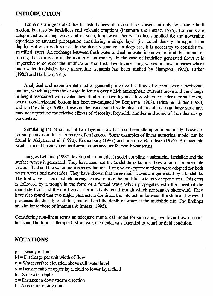
Tsunamis are generated due to disturbances of free surface caused not only by seismic fault motion, but also by landslides and volcanic eruptions (Imamura and Imteaz, 1995). Tsunamis are categorized as a long wave and as such, long wave theory has been applied for the governing equations of tsunami propagation considering a single layer (i.e. equal density throughout the depth). But even with respect to the density gradient in deep sea, it is necessary to consider the stratified layers. An exchange between fresh water and saline water is known to limit the amount of mixing that can occur at the mouth of an estuary. In the case of landslide generated flows it is imperative to consider the mudflow as stratified. Two-layered long waves or flows in cases where underwater landslides have generating tsunamis has been studied by Hampton (1972), Parker (1982) and Harbitz (1991).

Analytical and experimental studies generally involve the flow of current over a horizontal bottom, which neglects the change in terrain over which atmospheric currents move and the change in height associated with avalanches. Studies on two-layered flow which consider current flowing over a non-horizontal bottom has been investigated by Benjamin (1968), Britter & Linden (1980) and Lin Po-Ching (1990). However, the use of small-scale physical model to design large structures may not reproduce the relative effects of viscosity, Reynolds number and some of the other design parameters.

Simulating the behaviour of two-layered flow has also been attempted numerically, however, for simplicity non-linear terms are often ignored. Some examples of linear numerical model can be found in Akiyama et al. (1990), Kranenburg (1993) and Imamura & Imteaz (1995). But accurate results can not be expected until simulations account for non-linear terms.

Jiang & Leblond (1992) developed a numerical model coupling a submarine landslide and the surface waves it generated. They have assumed the landslide as laminar flow of an incompressible viscous fluid and the water motion as irrotational. Long wave approximations were adopted for both water waves and mudslides. They have shown that three main waves are generated by a landslide. The first wave is a crest which propagates away from the mudslide site into deeper water. This crest is followed by a trough in the form of a forced wave which propagates with the speed of the mudslide front and the third wave is a relatively small trough which propagates shoreward. They have also found that two major parameters dominate the interaction between the slide and waves it produces: the density of sliding material and the depth of water at the mudslide site. The findings are similar to those of Imamura & Imteaz (1995).

Considering non-linear terms an adequate numerical model for simulating two-layer flow on non- horizontal bottom is attempted. Moreover, the model was extended to actual or field condition.

NOTATIONS

p = Density of fluid M = Discharge per unit width of flow Il = Water surf ace elevation above still water level

a = Density ratio of upper layer fluid to lower layer fluid h = Still water depth x = Distance in downstream direction t = Axis representing time

g = Acceleration due to gravity i = Spatial node points in a finite difference scheme n = Temporal node points in a finite difference scheme l3 = Depths ratio of lower layer to upper layer k = Wave number L = Wave length a = wave amplitude

THEORETICAL BACKGROUND

A mathematical model for two-layer flow in a wide channel with non-horizontal bottom was ’ set up assuming a hydrostatic pressure distribution, negligible friction and negligible interfacial

mixing. Also uniform density and velocity distributions in each layer was assumed. Considering a two dimensional case as shown in Figure 1, using Euler’s equation of motion and continuity for each layer, by integrating the equations for specified limit of each layer and applying long wave approximation (i.e. vertical accelerations are negligible) and boundary conditions, following integrated governing equations were derived. The derivations are explained in details by Imteaz, M.A. ( 1994).

For upper layer- Mass conservation equation,

dMr+%-772) _(-) 3x at-

and momentum equation,

a~i+d(M?/Di)+~~,‘% -0 -- at 8x ax

For lower layer-

Mass conservation equation, - ~Mz+%-~ - - ax at

and momentum equation,

3M2+ d(M:/D2)+gD2 a’71 ah1 a’72

at ax ,C,-dx)+cp}=,

Where, r-l1 = Water surf ace elevation above still water level of layer ‘1’ rl2 = Water surf ace elevation above still water level of layer ‘2’

Dr=rll+hl-r12 DZ=h2+r12 ht = Still water depth of layer ‘1’ h2 = Still water depth of layer ‘2’

o = p1432

-hl+rl2

Ml = i’ uidy&I2= j u2dy -hi+rl2 -hl-h2

(1)

(2)

(3)

(4)

HI

H2

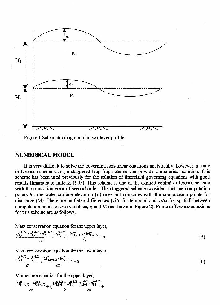
Figure 1 Schematic diagram of a two-layer profile

NUMERICAL MODEL

It is very difficult to solve the governing non-linear equations analytically, however, a finite difference scheme using a staggered leap-frog scheme can provide a numerical solution. This scheme has been used previously for the solution of linearized governing equations with good results (Imamura & Imteaz, 1995). This scheme is one of the explicit central difference scheme with the truncation error of second order. The staggered scheme considers that the computation points for the water surface elevation (IJ) does not coincides with the computation points for discharge (M). There are half step differences &At for temporal and %Ax for spatial) between computation points of two variables, rl and M (as shown in Figure 2). Finite difference equations for this scheme are as follows.

Mass conservation equation for the upper layer,

R,* n+l’* _ 71 ‘j’” - ‘I$“* + ~$2~~ + MF,i+lf2 - Mr,i_lf2 = o

At Ax

Mass conservation equation for the lower layer,

$;“* - $$‘* + @,i+i/2 _ M!,i-i/2 = o At Ax

Momentum equation for the upper layer,

(5)

(6)

MY,i+1/2 _ M n-l/* n-l/* @kl’* + Q ,i n-l/*

At + g 1,1+1 771,i+l -%,i +

2 Ax

(M&$ (Mfj!l,2 >*

CDFj!$ + D1 ,i n-1’2 + Dgf + D;j3’*)/4 _ (Dg’2 + Df;;2 + D;i3” + D, n-312 14

,- i_l ) 7 = 0

Ax

Momentum equation for the lower layer,

M!!,i+l/* - M ;$+I,* +

At

g (D;-$ + D;-j’*)

2

(#;+1,2)* (M;j!1,2 >*

(D;-;!; , +D2,i n-1/2 + D;-..f + ,

Ax

(7)

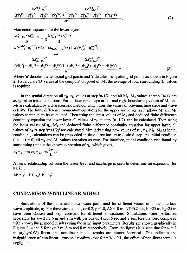
(8)

Where ‘n’ denotes the temporal grid points and ‘i’ denotes the spatial grid points as shown in Figure 2. To calculate ‘D’ values at the computation point of ‘M’, the average of four surrounding ‘D’ values is required.

In the spatial direction all IJ 1, II* values at step ‘n-1/2’ and all Mr, M2 values at step ‘(n- 1)’ are assigned as initial conditions. For all later time steps at left and right boundaries, values of Ml and M2 are calculated by a characteristic method, which uses the values of previous time steps and wave celerity. The finite difference momentum equations for the upper and lower layer allows Mr and M2 values at step ‘n’ to be calculated. Then using the latest values of Mz. and deduced finite difference continuity equation for lower layer all values of r)2 at step ‘(n+1/2)’ can be calculated. Then using the latest values of Q, Mr and deduced finite difference continuity equation for upper layer, all values of r-ii at step ‘(n+1/2)’ are calculated. Similarly using new values of qi, rl2, Mr, M2 as initial conditions, calculations can be proceeded in time direction up to desired step. As initial condition (i.e. at t = 0) all ~1 and Ml values are taken as zero. For interface, initial condition was found by substituting t = 0 in the known expression of Q, which gives,

2x 472=a2Sill(kX)=a2SiIl(-X)

L

A linear relationship between the water level and discharge is used to determine an expression for M2 i.e.,

M2 = &5&2(H2+~2)

COMPARISON WITH LINEAR MODEL

Simulations of the numerical model were performed for different values of initial interface wave amplitude, al. For these simulations, ~0.2, p=l .O, AX=10 m, AT=0.2 set, hr=25 m, h2=25 m have been chosen and kept constant for different simulations. Simulations were performed separately for a*= 2 m, 6 m and 8 m with periods of 4 set, 6 set and 8 sec. Results were compared with known linear model results using the same input parameters. Results are shown graphically in Figures 3,4 and 5 for a;! = 2 m, 6 m and 8 m respectively. From the figures it is seen that for a;? = 2 m (a2&=0.08) linear and non-linear model results are almost identical. This indicates the insignificance of non-linear terms and confirms that for r-l/l-r < 0.1, the effect of non-linear terms is negligible.

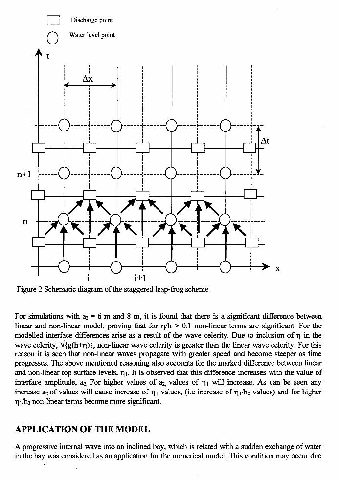
0 Discharge point

0 Water level point

n I f?

i m____ --..--~------ _____+_____ 4

X

Figure 2 Schematic diagram of the staggered leap-frog scheme

For simulations with a:! = 6 m and 8 m, it is found that there is a significant difference between linear and non-linear model, proving that for q/h > 0.1 non-linear terms are significant. For the modelled interface differences arise as a result of the wave celerity. Due to inclusion of q in the wave celerity, 4{ g(h+q)} , non-linear wave celerity is greater than the linear wave celerity. For this reason it is seen that non-linear waves propagate with greater speed and become steeper as time progresses. The above mentioned reasoning also accounts for the marked difference between linear and non-linear top surface levels, q 1. It is observed that this difference increases with the value of interface amplitude, a2. For higher values of q, values of qi will increase. As can be seen any increase a;! of values will cause increase of qi values, (i.e increase of qi/h2 values) and for higher q i/h2 non-linear terms become more significant.

APPLICATION OF THE MODEL

A progressive internal wave into an inclined bay, which is related with a sudden exchange of water in the bay was considered as an application for the numerical model. This condition may occur due

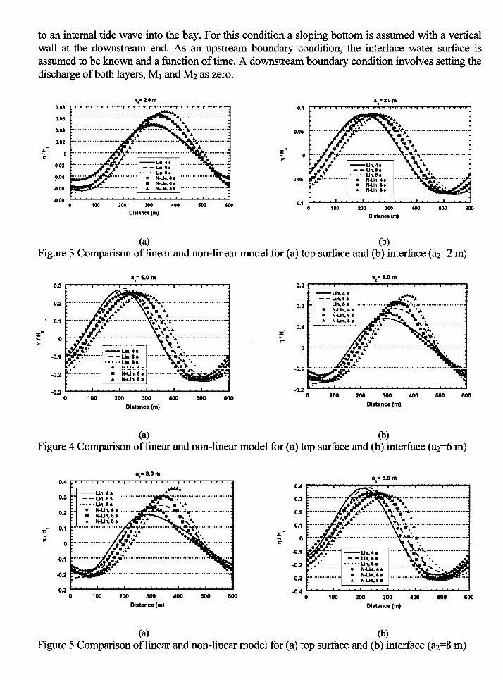
to an internal tide wave into the bay. For this condition a sloping bottom is assumed with a vertical wall at the downstream end. As an upstream boundary condition, the interface water surface is assumed to be known and a function of time. A downstream boundary condition involves setting the discharge of both layers, Ml and M2 as zero.

0.05

0.06

0.04

0.02

0

-0.02

-9.04

-0.05

0.1

0.05

0

-0.05

-0.1 4.05 t.‘..‘..‘.‘....‘....‘..‘.‘....’

0 .I00 200 300 400 500 600

Di6hnc6 (m) 0 100 200 306 400 500 500

Di6tmc6 (III)

(4 @I Figure 3 Comparison of linear and non-linear model for (a) top surface and (b) interface (a2=2 m)

*z= 6.0 m 0.3 1. . . . I . . . ’ I . . * . I . . . . I . * . . I . * 7 0.3

0.2

0.1

0

-0.1

-0.2

0.2

0.1

0

-0.1

d-l?

I” F

0.3t..““‘““““““““““.” 0 100 200 300 400 500 600

Distance (m)

.:... . . . . . . . . . . . . . . . . . . . . -“.a

0 100 200 300 400 500 600

Distance(m)

(a> 09 Figure 4 Comparison of linear and non-linear model for (a) top surface and (b) interface (a2=6 m)

0.4

0.3

0.2

0.1

0

-0.1

-0.2

s,= 8.0 m

0.4

0.3

0.2

0.1

0

0.1

-0.2

-0.3

I- E

I” F

p . . . . . . . . . . . . . . . . . . . . . . . . . . . . . . . . . T..\&L . . . . . . . . . . . . . . . . . . . . . . . . . . hi ,....................... .l

0.3F....“...‘..‘.‘....“...‘..‘.~ 0 100 200 300 400 300 600

Distance(m)

I ..4~...“.‘..‘....‘..“‘....l....~

0 100 200 300 400 500 600

(4 09 Figure 5 Comparison of linear and non-linear model for (a) top surface and (b) interface (a2=8 m)

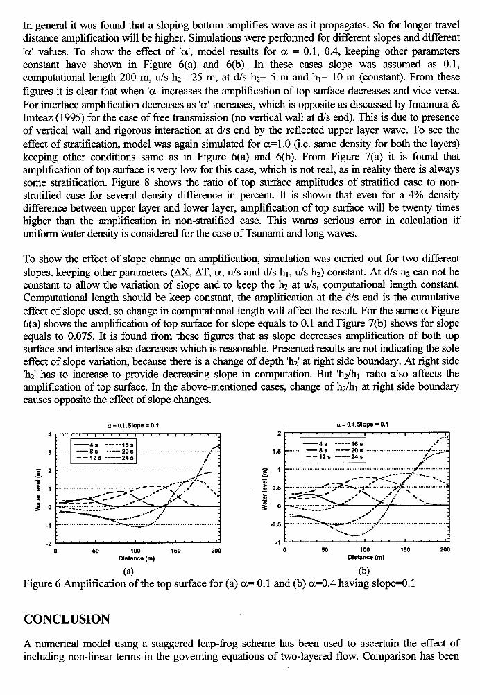
In general it was found that a sloping bottom amplifies wave as it propagates. So for longer travel distance amplification will be higher. Simulations were performed for different slopes and different

‘a’ values. To show the effect of ‘a’, model results for a = 0.1, 0.4, keeping other parameters constant have shown in Figure 6(a) and 6(b). In these cases slope was assumed as 0.1, computational length 200 m, u/s hz= 25 m, at d/s hz= 5 m and hi= 10 m (constant). From these

figures it is clear that when ‘o? increases the amplification of top surface decreases and vice versa. For interface amplification decreases as ‘a’ increases, which is opposite as discussed by Imamura & Imteaz (1995) for the case of free transmission (no vertical wall at d/s end). This is due to presence of vertical wall and rigorous interaction at d/s end by the reflected upper layer wave. To see the effect of stratification, model was again simulated for a=1 .O (i.e. same density for both the layers) keeping other conditions same as in Figure 6(a) and 6(b). From Figure 7(a) it is found that amplification of top surface is very low for this case, which is not real, as in reality there is always some stratification. Figure 8 shows the ratio of top surface amplitudes of stratified case to non- stratified case for several density difference in percent. It is shown that even for a 4% density difference between upper layer and lower layer, amplification of top surface will be twenty times higher than the amplification in non-stratified case. This warns serious error in calculation if uniform water density is considered for the case of Tsunami and long waves.

To show the effect of slope change on amplification, simulation was carried out for two different slopes, keeping other parameters (AX, AT, a, u/s and d/s hi, u/s h2) constant. At d/s h2 can not be constant to allow the variation of slope and to keep the h2 at u/s, computational length constant. Computational length should be keep constant, the amplification at the d/s end is the cumulative effect of slope used, so change in computational length will affect the result. For the same a Figure 6(a) shows the amplification of top surface for slope equals to 0.1 and Figure 7(b) shows for slope equals to 0.075. It is found from these figures that as slope decreases amplification of both top surface and interface also decreases which is reasonable. Presented results are not indicating the sole effect of slope variation, because there is a change of depth ‘h2’ at right side boundary. At right side ‘hi has to increase to provide decreasing slope in computation. But ‘h&’ ratio also affects the amplification of top surface. In the above-mentioned cases, change of h2/hi at right side boundary causes opposite the effect of slope changes.

a=0.1,Sl0pe=0.1 a = 0.4,Slopa = 0.1

. . . . . . . ;;’

: . _ . . . . . . . .j.. . _ % 2.

f . .-P-‘---;

, - _ . . . . . -_.LG.y.” ~’ ..+p,

= - a.C...::. ‘p.. . .A.;. _

E :

~’ : \

.H _ _ c - -_--

s OF---

\..-- :5* _.-- ._ /’ . ~ .~ .~ ;: -..........--

. =-----+w #/’ J

\____.’ _/- / _, _ . . . . . . . . ..b....~~~_.~*..-~.. . . . . . . . . . . . . . :

-2 . . . .‘. . . ‘I* * * *‘. . *. ’ 0 50 100 150 200 0 50 100 150

Distance (m) Distance (m)

(a> @I

Figure 6 Amplification of the top surface for (a) a= 0.1 and (b) a=0.4 having slope=O.l

CONCLUSION

A numerical model using a staggered leap-frog scheme has been used to ascertain the effect of including non-linear terms in the governing equations of two-layered flow. Comparison has been

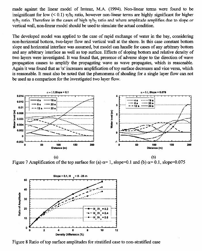
made against the linear model of Imteaz, M.A. (1994). Non-linear terms were found to be insignificant for low (< 0.1) q/h2 ratio, however non-linear terms are highly significant for higher n/h2 ratio. Therefore in the cases of high q/h2 ratio and where amplitude amplifies due to slope or vertical wall, non-linear model should be used to simulate the actual condition.

The developed model was applied to the case of rapid exchange of water in the bay, considering non-horizontal bottom, two-layer flow and vertical wall at the shore. In this case constant bottom slope and horizontal interface was assumed, but model can handle for cases of any arbitrary bottom and any arbitrary interface as well as top surface. Effects of sloping bottom and relative density of two layers were investigated. It was found that, presence of adverse slope to the direction of wave propagation causes to amplify the propagating wave as wave propagates, which is reasonable. Again it was found that as ‘o? increases amplification of top surface decreases and vice versa, which is reasonable. It must also be noted that the phenomena of shoaling for a single layer flow can not be used as a comparison for the investigated two layer flow.

0.014

0.012

0.01

z 0.008 P B 0.006 L

j 0.004

a = 1.0,Slope = 0.1 4

-1

a = 0.1, Slope = 0.076

r.. . . #.. ---.. . . ?.-&. . . .I.. . .~i _..-

0 50 100 150 200 0 50 100 150 200 Dietence (m) Dletence (m)

(a) (b) Figure 7 Amplification of the top surface for (a) ct= 1, slope=O.l and (b) a= 0.1, slope=0.075

Slope = 0.1, H 1 = 5 - 25 m

I . . . I . . . I . . . I . . . I . . . 0 2 4 6 a 10 12

Density Difference (X)

Figure 8 Ratio of top surface amplitudes for stratified case to non-stratified case

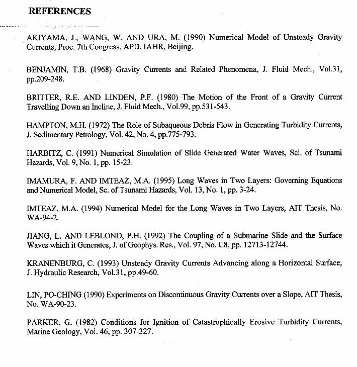
REFERENCES

, AIUYAMA, J., WANG, W. AND URA, M. (1990) Numerical Model of Unsteady Gravity Currents, Proc. 7th Congress, APD, IAHR, Beijing.

BENJAMIN, T.B. (1968) Gravity Currents and Related Phenomena, J. Fluid Mech., Vol.3 1, pp.209-248.

BRITTER, R.E. AND LINDEN, P.F. (1980) The Motion of the Front of a Gravity Current Travelling Down an Incline, J. Fluid Mech., Vo1.99, pp.53 l-543.

HAMPTON, M.H. (1972) The Role of Subaqueous Debris Flow in Generating Turbidity Currents, J. Sedimentary Petrology, Vol. 42, No. 4, pp.775-793.

HARBITZ, C. (1991) Numerical Simulation of Slide Generated Water Waves, Sci. of Tsunami Hazards, Vol. 9, No. 1, pp. 15-23.

IMAMURA, F. AND IMTEAZ, M.A. (1995) Long Waves in Two Layers: Governing Equations and Numerical Model, SC. of Tsunami Hazards, Vol. 13, No. 1, pp. 3-24.

IMTEAZ, M.A. (1994) Numerical Model for the Long Waves in Two Layers, AIT Thesis, No. WA-94-2.

JIANG, L. AND LEBLOND, P.H. (1992) The Coupling of a Submarine Slide and the Surface Waves which it Generates, J. of Geophys. Res., Vol. 97, No. C8, pp. 12713-12744.

KRANENBURG, C. (1993) Unsteady Gravity Currents Advancing along a Horizontal Surface, J. Hydraulic Research, Vol.3 1, pp.49-60.

LIN, PO-CHING (1990) Experiments on Discontinuous Gravity Currents over a Slope, AIT Thesis, No. WA-90-23.

PARKER, G. (1982) Conditions for Ignition of Catastrophically Erosive Turbidity Currents, Marine Geology, Vol. 46, pp. 307-327.

Science of Tsunami Hazards Volume 19, pages 150-170 (2001)

MODELING THE LA PALMA LANDSLIDE TSUNAMI

Charles L. Mader

Mader Consulting Co.

Honolulu, Hawaii USA

ABSTRACT

The tsunami expected from a lateral collapse of the Cumbre Vieja Volcano on La Palmain the Canary Islands was modeled. The flank collapse for a ‘worst case” landslide wasmodeled as a 650 meter high, 20 kilometer radius water wave after 30 kilometers of travelas predicted by physical modeling studies of Fritz at ETH in Zurich, Switzerland.

The modeling was performed using the SWAN code which solves the nonlinear longwaver equations. The tsunami generation and propagation was modeled using a 10 minuteMercator grid of 600 by 640 cells. The small wavelength and period of the tsunami expectedfrom the landslide source results in an intermediate wave rather than a shallow watertsunami wave. The use of a shallow water model only describes the geometric spreasingof the wave and not the significant dispersion such a short period wave would exhibit.Dispersion would reduce the wave amplitudes to less than one-third of the shallow wateramplitudes.

The upper limit shallow water modeling indicates that the east coast of the U.S.A. andthe Caribbean would receive tsunami waves less than 3 meters high. The European andAfrican coasts would have waves less than 10 meters high.

Full Navier-Stokes modeling including dispersion and geometric spreading for the Fritzinitial wave profile predicts that the maximim wave amplitude off the U.S. east coast wouldbe about a meter. Even with shoaling the wave would not present a significant hazard.

Science of Tsunami Hazards Volume 19, pages 150-170 (2001)

INTRODUCTION

The lateral collapse of the flank of the Cumbre Vieja Volcano on La Palma in theCanary Islands represents the ”worst case” La Palma submarine landslide. This LaPalma slide involves 500 cubic kilometers of material runing out 60 kilometers at a meanspeed of 100 meters/second. Hermann Fritz of the Swiss Federal Institute of Technology(ETH) in Zurich, Switzerland has physically modeled the landslide as one single block anddetermined that the landslide would generate a 650 meter high wave with a wavelength of30 to 40 kilometers and period of 3 to 4 minutes. The wave profile he obtained is shown inFigure 1. It was measured after the wave had effectively traveled 30 kilometers or about0.04 hours from the source.

He states that such a wave is not a shallow water tsunami wave but an intermediatewave that would undergo significant dispersion as it propagated away from the sourceregion. The experimental apparatus created by Fritz and used to physically model the LaPalma landslide is described in reference 1.

If one considers only geometric spreading in a constant depth basin then to an upperlimit approximation the wave height as a function of distance from the source would be

H = HoRo

R

where Ro is the initial source radius, R is the distance the wave has traveled from thesource, and Ho is the initial height of the source. For the La Palma event Ro is 20kilometers, and Ho is 650 meters. The wave height after 1000 kilometers of travel is 13meters, after 5000 kilometers is 2.6 meters and after 10,000 kilometers is 1.3 meters.

To obtain another estimate of the effect of geometric spreading throughout the AtlanticOcean and of the upper limit wave amplitude, shallow water numerical modeling wasperformed using the actual depths throughout the Atlantic Ocean.

In addition to geometric spreading the short wavelength and short period wave wouldundergo significant dispersion as it traveled. To a first approximation dispersion wouldreduce the heights to less than one-third of the above values as shown in reference 2 and3 and discussed in the section on dispersion modeling.

For comparision, the great Lisbon tsunami was caused by the November 1, 1755earthquake generated a tsunami which arrived at Lisbon between 40 minutes and onehour after the earthquake as a withdrawing wave that emptied the Lisbon Oeiras Bay tomore than a mile out. Then a tsunami wave with an amplitude of about 20 meters arrivedfollowed by two more waves about an hour apart. The tsunami wave had a period ofone hour and amplitude of up to 20 meters at Lisbon and along the African and southEuropean coasts, of 4 meters along the English coast, and of 7 meters at Saba in WestIndies after 7 hours of travel. To reproduce the observed tsunami wave characteristics asource source 300 kilometers in radius with a drop of 30 meters is required to be locatedin the region of the 1969 earthquake near the Gorringe bank as described in reference 4.

The May 23, 1960 Chile earthquake had a magnitude of 8.5 and generated a tsunamiwith a 25 minute period from a source about 150 kilometers wide and 800 kilometers longor 120,000 sq kilometers. The March 26, 1964 Alaskan earthquake near Prince Williamsound had a magnitude of 8.4 and generated a tsunami wave with a 30 minute period froma source about 300 kilometers wide and 800 kilometers long or 240,000 square kilometers.

To a first approximation the tsunami wave period is determined primarily by the width ofthe ocean floor displaced by the earthquake and the wave amplitude by the height of theocean floor displacement.

SHALLOW WATER MODELING

The modeling was performed using the SWAN non-linear shallow water code whichincludes Coriolis and frictional effects. The SWAN code is described in Reference 5. Thecalculations were performed on 866 Mhz Pentium personal computers with 128 megabytesof memory.

The 10 minute Atlantic topography was generated from the 2 minute Mercator GlobalMarine Gravity topography of the earth of Sandwell and Smith of the Scripps Institute ofOceanography and described in Reference 6. The grid was 600 by 640 cells with the lefthand corner at 20 S, 100 W. The grid extended from 20 N to 65 N and from 100 W to 0W. The time step was 10 seconds.

The source used in the calculations was a 20 kilometer radius of 650 meter high waterlocated near La Palma island. This source is the same height but larger in area than theFritz wave shown in Figure 1.

The Table 1 locations are shown in Figure 2. The units of the X and Y axis are 10kilometers. The travel time chart is shown in Figure 3.

The maximum deep water amplitudes at various locations are given in Table 1. Thepositive wave arrives first followed by several waves with the first wave usually having themaximum amplitude.

As shown in Reference 5 the run-up amplification may be from 2 to 3 times the deepwater wave amplitude. Locations with depths less than 1000 meters have some of the run-up amplification included. Dispersion would reduce the wave amplitudes by more than therun-up amplification so the upper limit amplitudes in Table 1 are also upper limit valuesafter run-up.

The east coast of the U.S.A. and the Caribbean receive a tsunami wave with an upperlimit less than 3 meters high. The European and African coasts receive a tsunami with anupper limit less than 10 meters high.

Computer generated animations of these calculations are available athttp://t14web.lanl.gov/Staff/clm/tsunami.mve/tsunami.htm.

The use of a shallow water model to describe the propagation of waves that are reallyintermediate water waves dispersing to deep water waves as they travel can only furnishan upper limit estimate of the amplitude and period of the waves. To obtain more realisticwave characteristics a full Navier-Stokes model is needed.

The assumption that the Fritz wave represents the initial displacement at the source isan approximation that needs to improved as the wave was actually equivalent to the waveafter it had traveled 30 kilometers of 0.0376 hours. An initial displacement was determinedthat would approximately reproduce the Fritz wave at 30 kilometers and the calculationsrepeated to obtain a more realistic model.

DISPERSION MODELING

To obtain an estimation of the effect of dispersion the procedures described in reference5 were used.

The linear gravity wave model solves the two-dimensional linear gravity wave with aGaussian or a square wave displacement using Fourier transforms for any time of interest.The wave description is obtained for any uniform length, density, gravity and Gaussianbreak width or square wave half-width. The model is two-dimensional and symmetricalabout the center of the initial displacement, only half of the wave profile is calculated andthus the dispersion effects are described without any geometric spreading.

To model the dispersion effects for the case modeled previously using the SWAN code,a 650 meter high, 20 kilometer square half-width, water displacement in 5000 meter deepwater was studied. The initial profile and the wave at 0.5, 2.0, 5.0 and 10.0 hours (400,1600, 4000, 8000 km) are shown in Figure 5. The wave disperses into a train of waves witha maximum amplitude of 320, 220, 180, 150 meters or from one-half to one-fourth of theinitial wave amplitude.

A 650 meter high Gaussian surface water displacement in 5000 meter deep water withGaussian break of 10km (which is equivalent to an Airy wave with a half-wavelength of45 kilometers) is a good approximation of the Fritz wave shown in Figure 1. The initialprofile and the wave at 0.5, 2.0, 5.0 and 10.0 hours (400, 1600, 4000, 8000 km) are shownin Figure 5. The wave disperses into a train of waves with a maximum amplitude of 220,150, 110, 90 meters or from one-third to one-eighth of the initial wave amplitude.

The ZUNI code solves the two-dimensional time dependent Navier-Stokes equations forincompressible flow and is described in detail in reference 5.

To approximate the Fritz wave shown in Figure 3, a 650 meter high Airy wave surfacewater displacement in 5050 meter deep water with with a half-wavelength of 40 kilometerswas modeled using ZUNI for 3000 kilometers of travel. The calculations for this geometrywere performed with 15 cells in the Y or depth direction and 5000 cells in the R or radialdirection. The cells were 500 meters high in the Y direction and 1000 meters long in theradial direction. The time step was 0.1 seconds. These calculations are an extension ofthose described in references 2, 3, and 5.

The calculated wave profiles are shown in Figure 6 after various times and distanceof travel. The calculated wave amplitude as a function of time and distance is shown inTable 2. The wave amplitude with geometric spreading and diffusion has been reduced to2.6 meters after 2500 kilometers of travel. The wave amplitude after 10,000 kilometers oftravel would be about half a meter.

FRITZ SOURCE AT 30 KM MODEL

The Fritz wave in Figure 1 was measured by a gauge in front of the landslide that wasat an equivalent location of 30 kilometers from the slide.

In the previous study the source was described as a displacement of water with thegeometry of the Fritz wave and centered at the source. The wave observed by Fritz was2-D and would not exhibit geometric spreading like a 3-D one with distance of travel.The 2-D linear gravity wave model has 320 meters amplitude after 24 km of travel for theGaussian wave and 460 meters for the square wave. To more closely approximate the waveFritz observed at 30 km, the initial 40 km diameter square displacement amplitude needsto be increased to 990 meters as shown in Figure 7 and the Gaussian displacement to 1400meters as shown in Figure 8.

Using the linear gravity model to model the dispersion effects without geometric

spreading, the wave profile at 0.5, 2.0, 5.0 and 10 hours are shown in Figures 9 and10. The amplitudes are increased by a factor of about 2.0 for the Gaussian model and afactor of about 1.4 for the square displacement over those of Figures 4 and 5.

Using the square displacement with a 990 meter initial height that gave anapproximately 650 meter high wave at 30 km, the SWAN calculation gave the wave heightsshown in Table 3 which are about 1.52 times higher than those of Table 1. Using the Airydisplacement with a 1400 meter initial height that gave an approximately 650 high waveat 30 km, the ZUNI calculation gave the wave heights shown in Table 4 which are about2.15 times larger than those of Table 2. The wave profiles as a function of distance areshown in Figure 11. The wave amplitude off the U.S. coast would be less than one meter.Even with shoaling the wave would not present a significant hazard.

REFERENCES

1. Hermann M. Fritz, Willi H. Hager and Hans-Erwin Minor Lituya Bay Case: RockslideImpact and Wave Run-Up , Science of Tsunami Hazards, 19, 3-22 (2001).

2. Charles L. Mader, Dennis W. Moore, George F. Carrier Numerical Tsunami PropagationStudy - III, Science of Tsunami Hazards, 11, 93-106 (1993).

3. David A. Crawford and Charles L. Mader, Modeling Asteroid Impact and Tsunami ,Science of Tsunami Hazards, 16, 21-30 (1998).

4. Charles L. Mader, Modeling The 1755 Lisbon Tsunami , Science of Tsunami Hazards,19, 93-116 (2001).

5. Charles L. Mader Numerical Modeling of Water Waves, University of California Press,Berkeley, California (1988).

6. W. H. F. Smith and D. T. Sandwell, Global Seafloor Topography from Satellite Altimetryand Ship Depth Soundings, Science, April 7, 1997.

TABLE 1UPPER LIMIT WAVE HEIGHTS

FOR FRITZ LA PALMA TSUNAMI

Maximum MinimumNo Depth Location Amplitude Amplitude

Meters Meters Meters1 953 Off Lisbon +9.0 -10.2 4747 East of Saba +2.2 -2.23 825 East of Saba +2.0 -1.94 3446 North of San Juan +1.8 -1.65 783 East of Miami +0.3 -0.26 2922 East of Washington +3.0 -3.07 178 South West of England +2.5 -1.9

8 4574 West of Lisbon +5.0 -5.09 3868 West of Lagos +4.0 -2.0

10 3923 West of Gibraltar +6.0 -5.011 4376 West of Gibraltar +6.0 -4.012 1717 West of Casablanca +7.0 -4.013 3314 N-W of Source +8.0 -6.0

DISPERSION WOULD REDUCE HEIGHTS TO

LESS THAN ONE THIRD OF ABOVE VALUES

TABLE 2ZUNI WAVE HEIGHTS

FOR FRITZ LA PALMA TSUNAMI

No Time Radial Distance Amplitude Amp/650.Hours Meters Meters Percent

1 .03 24,000 170. 26.2 .05 40,000 120. 18.3 .10 80,000 71. 11.4 .125 100,000 60. 9.25 .250 200,000 30. 4.66 .625 500,000 14. 2.17 1.25 1,000,000 7.0 1.18 1.88 1,500,000 4.6 0.719 2.50 2,000,000 3.4 0.52

10 3.12 2,500,000 2.6 0.4

TABLE 3WAVE HEIGHTS

FOR FRITZ LA PALMA TSUNAMI AT 30KM

Maximum MinimumNo Depth Location Amplitude Amplitude

Meters Meters Meters1 953 Off Lisbon +14.0 -15.2 4747 East of Saba +3.2 -3.03 825 East of Saba +2.9 -2.54 3446 North of San Juan +2.2 -2.05 783 East of Miami +0.7 -0.56 2922 East of Washington +4.1 -4.07 178 South West of England +3.5 -2.0

8 4574 West of Lisbon +7.0 -8.09 3868 West of Lagos +6.0 -3.0

10 3923 West of Gibraltar +8.0 -7.011 4376 West of Gibraltar +8.0 -6.012 1717 West of Casablanca +10.0 -6.013 3314 N-W of Source +12.0 -9.0

DISPERSION WOULD REDUCE HEIGHTS TO

LESS THAN ONE THIRD OF ABOVE VALUES

TABLE 4ZUNI WAVE HEIGHTS

FOR FRITZ LA PALMA TSUNAMI AT 30 KM

No Time Radial Distance Amplitude Amp/1400.Hours Meters Meters Percent

1 .03 24,000 370. 26.2 .05 40,000 272. 19.3 .10 80,000 160. 11.4 .125 100,000 133. 9.55 .250 200,000 70. 5.06 .625 500,000 30. 2.17 1.25 1,000,000 15.0 1.18 2.50 2,000,000 7.3 0.52

9 4.03 3,228,000 4.2 0.3010 5.00 4,005,000 3.2 0.2111 5.70 4,565,700 2.6 0.18

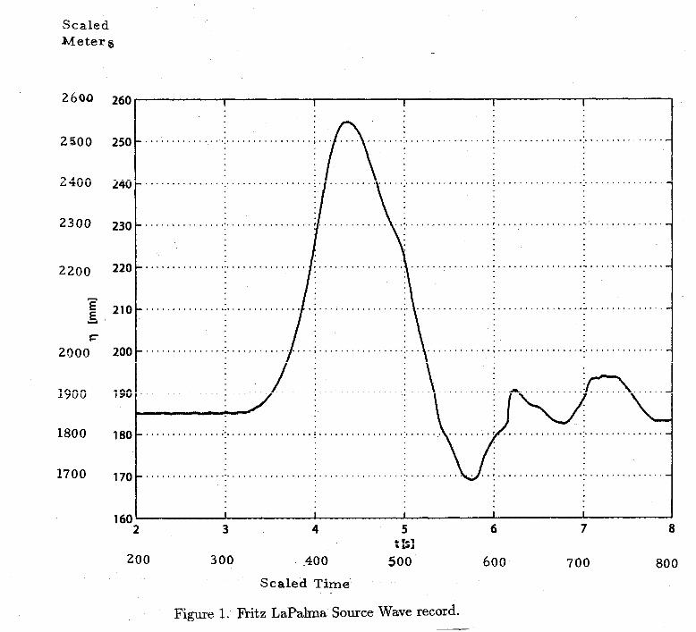
2600 260

2500 250

Scaled Meter5

2400 240

2300 230

2200 220

z 6 F

2000

210

1900

1800

1700

180

I I 1 I I

200

3 4

300 .400

5

trsl

500

Scaled Time

6

600

7

700

8

800

Figure 1. Fritz LaPalma Source Wave record.

0 200 400 600 800 1000 1200 1400 X

Y

0 200 400 600 800 loo0 1200 1400 X

Figure 2. The source region and Table 1 locations. The X and Y axis units are

kilometpr

1*

10

ICXX

Y

aoc

6OC

4Oc

2Cx

C

: - - _

I

’ I Figure 3. The travel time chart at one hour intervals.

W

6 E

E! I

: T

2M

(

HTK = 20,OOo - 0.0 ,“..,....,....,....I..‘.1

0.00 0.02 0.04 0.06

. .

Figure 4. The wave profile in meters &s a functisn of distance for a 650 meter high squtie displacement of water with a 20 kilometer half-width in 5000 meter deep water’: The linear gravity model is used which models dispersion with no geometrical spreading.

,

HTK = : 20,000 - 0.0, 0.5, 2, 5, IO I-R

E

F I

E T

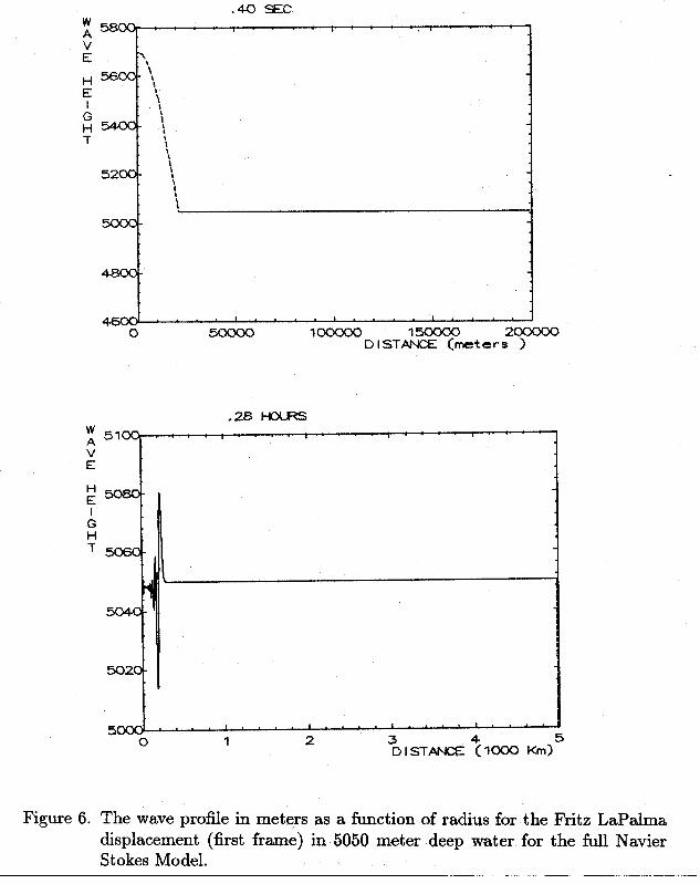
moooQ 15oooo 2#000 DISTANCE (meters )

.28 l-KxF?S

~5loq ‘1.. I.. . . 1.. ‘. *. . ‘. ” . . .

:

F=, I

Pi T 5060-

5020 -

Figure 6. The wave profile in meters as a function of radius for the Fritz LaPalma displacement (first frame) in 5050 meter deep water for the full Navier Stokes Model.

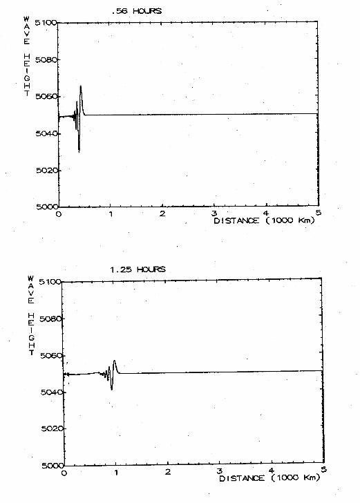
.56 l--Dms ‘. - 1.. : I. ‘. . 1 ‘. . I.. . .

I . . ..I . . ..‘..a. tn. . .

0 1 2 3 5 DISTANCE

&OO Km)

1.25 HOAS

H E I

ifi T

2.50 HOURS

~~...-.‘..-“.‘-.‘.‘. :

H 5054: E I

g 5052.;. T

5050

5048 i

0 1 2 3 DISTANCE &XI0 Km)

5

3 DISTANCE

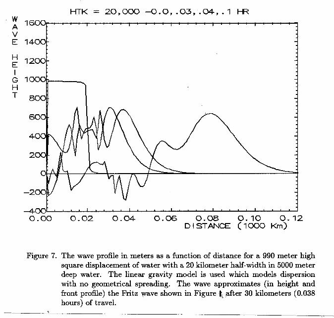
-201

Figure 7. The wave profile in meters as a function of distance for a 990 meter high square displacement of water with a 20 kilometer half-width in 5000 meter deep water. The linear gravity model is used which models dispersion with no geometrical spreading. The wave approximates (in height and front profile) the Fritz wave shown in Figure & after 30 kilometers (0.038 hours) of travel.

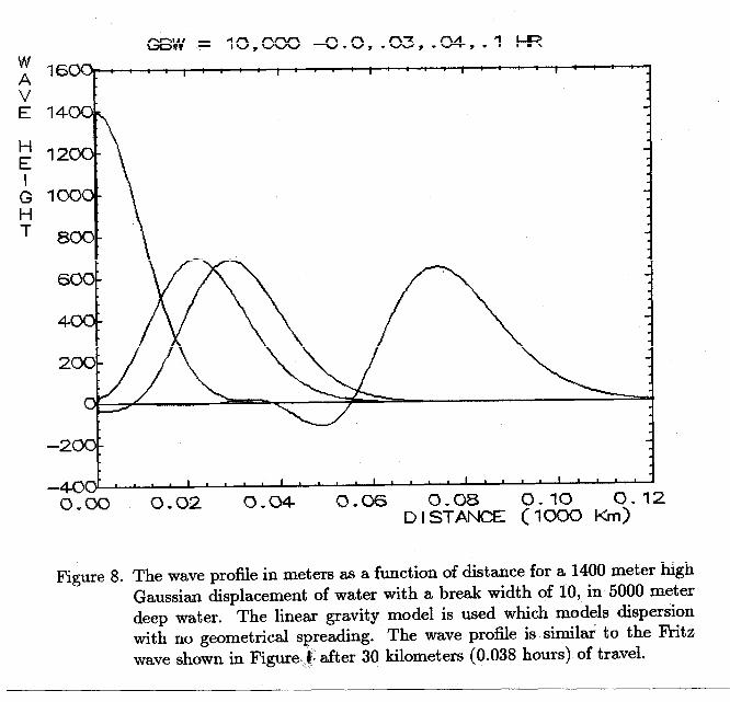
H E I

PI T

0.02 0.w 0.06 DISTANCE (loo0 Km)

Figure 8. The wave profile in meters as a function of distance for a 1400 meter high Gaussian displacement of water with a break width of 10, in 5000 meter deep water. The linear gravity model is used which models dispersion with no geometrical spreading. The wave profile is similar to the Fritz

wave shown in Figure.{: after 30 kilometers (0.038 hours) of travel.

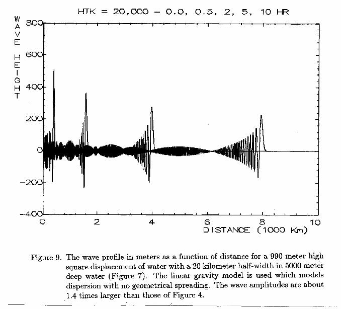
-2oc

-4ix I, I I I I , , , , , , , , , , , , , , ,

cl 2 4 D”I STANCE (z(1M30 Km)

IO

Figure 9. The wave profile in meters as a function of distance for a 990 meter high square displacement of water with a 20 kilometer half-width in 5000 meter deep water (Figure 7). The linear gravity model is used which models dispersion with no geometrical spreading. The wave amplitudes are about

1.4 times larger than those of Figure 4.

2 4 l?ISTANCE (“lOO0 Km)

IO

Figure 10. The wave profile in meters as a function of distance for a 1400 meter high Gaussian displacement of water with a Gaussian break length of 10 in 5000 meter deep water (Figure 8). The linear gravity model is used which models dispersion with no geometrical spreading. The wave amplitudes are about twice those of Figure 5.

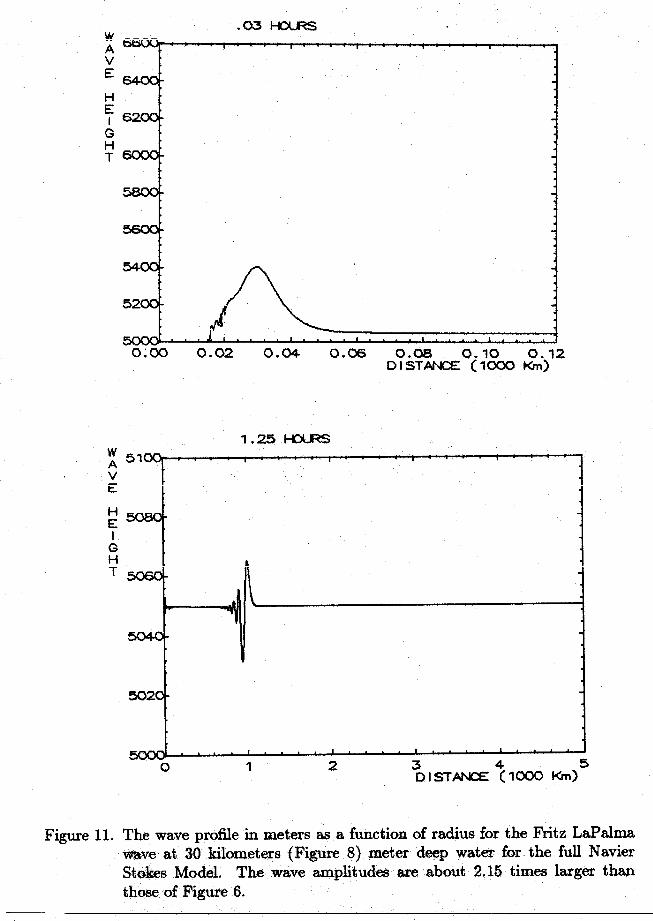
0:OO 0.02 0.04 0.06 0.12 DEiELE”(;& Km)

I . . . . I.. . * 1. * * ‘1’ * *.

0 1 2 3 &DO 5 DISTANCE fi)

Figure 11. The wave profile in meters as a function of radius for the Fritz LaPalma at 30 kilometers (Figure 8) meter deep water for the full Navier

Stokes Model. The wave amplitudes are about 2.15 times larger than those of Figure 6.

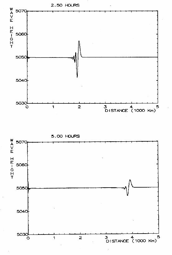
2.50 l4DmS

0 1 2 3 5 DISTANCE

&DO Kim)

1 507c

:

F I-

G

‘:

5044

5.00 HOURS

_ 3 DISTANCE “(I- Km)

3

BOOK REVIEW

The Big One -The Next California Earthquake

George Pararas-Carayannis

ISBN EB00014428

Forbes Press - - Honolulu, HI 96815

e-mail - forbes@forbesint.com

Don’t be turned off by the popularized style of the title or book.Pararas-Caryannis leads the reader - professional or layman - through adetailed background covering earthquakes, tsunamis, California geographyand history, seismology, then finally summarizing factually the odds ofmajor earthquakes in likely localities. And he does so in terms that allof us can understand and appreciate.

The author notes that he ”will provide answers to reasonable questionsby people concerned about their safety” and accomplishes that factuallyand in fact without sensationalism. Using a brief question and long answerformat, this is actually a treatise on earthquakes and related natural hazardsworldwide, with realistic scenarios of probable disasters in California.

There are several useful appendices and an extensive glossary (I learneda couple new terms) which are helpful and enlighting. I recommend thisbook.

Reviewed by George D. CurtisAffiliate Professor of Natural Sciences

University of Hawaii, Hilo, Hawaii