The Interior Transmission Problem -...
44
Introduction Transmission Eigenvalues Anisotropic media Numerical Examples Conclusion The Interior Transmission Problem Peter Monk (with Fioralba Cakoni and David Colton) Department of Mathematical Sciences University of Delaware Research supported in part by AFOSR
Transcript of The Interior Transmission Problem -...

Introduction Transmission Eigenvalues Anisotropic media Numerical Examples Conclusion
The Interior Transmission Problem
Peter Monk (with Fioralba Cakoni and David Colton)
Department of Mathematical SciencesUniversity of Delaware
Research supported in part by AFOSR
Introduction Transmission Eigenvalues Anisotropic media Numerical Examples Conclusion
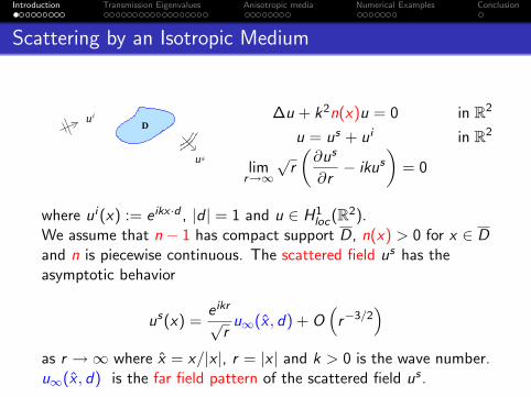
Scattering by an Isotropic Medium
u
s
Di
u
∆u + k2n(x)u = 0 in R2
u = us + ui in R2
limr→∞
√r
(∂us
∂r− ikus
)= 0
where ui (x) := e ikx ·d , |d | = 1 and u ∈ H1loc(R2).
We assume that n − 1 has compact support D, n(x) > 0 for x ∈ Dand n is piecewise continuous. The scattered field us has theasymptotic behavior
us(x) =e ikr
√ru∞(x , d) + O
(r−3/2
)as r →∞ where x = x/|x |, r = |x | and k > 0 is the wave number.u∞(x , d) is the far field pattern of the scattered field us .

Introduction Transmission Eigenvalues Anisotropic media Numerical Examples Conclusion
The Far Field Operator
Let Ω := x : |x | = 1 and define the far field operatorF : L2(Ω) → L2(Ω) by
(Fg)(x) :=
∫Ω
u∞(x , d)g(d)ds(d).
For z ∈ D the far field equation is
(Fg)(x) = Φ∞(x , z), g ∈ L2(Ω)
where
Φ∞(x , z) =e iπ/4
√8πk
e−ikx ·z
is the far field pattern of the fundamental solution
Φ(x , z) := i4H
(1)0 (k|x − z |) .
Introduction Transmission Eigenvalues Anisotropic media Numerical Examples Conclusion
Towards the Interior Transmission Problem
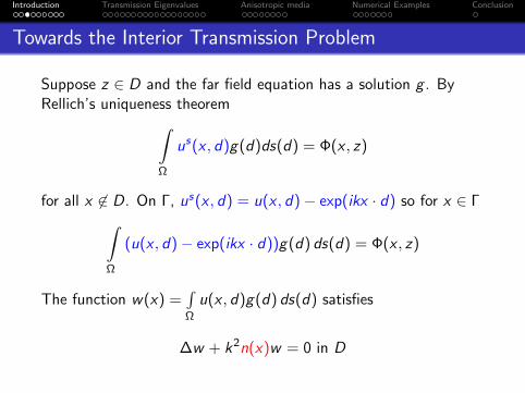
Suppose z ∈ D and the far field equation has a solution g . ByRellich’s uniqueness theorem∫
Ω
us(x , d)g(d)ds(d) = Φ(x , z)
for all x 6∈ D. On Γ, us(x , d) = u(x , d)− exp(ikx · d) so for x ∈ Γ∫Ω
(u(x , d)− exp(ikx · d))g(d) ds(d) = Φ(x , z)
The function w(x) =∫Ω
u(x , d)g(d) ds(d) satisfies
∆w + k2n(x)w = 0 in D

Introduction Transmission Eigenvalues Anisotropic media Numerical Examples Conclusion
Further towards the Interior Transmission Problem
The Herglotz wave function
v(x) =
∫Ω
exp(ikx · d)g(d) ds(d)
is an entire solution of the Helmholtz equation
∆v + k2v = 0 in R2
Since w − v = Φ outside D we obtain the boundary conditions
w − v = Φ on Γ∂
∂ν(w − v) =
∂
∂νΦ
Introduction Transmission Eigenvalues Anisotropic media Numerical Examples Conclusion
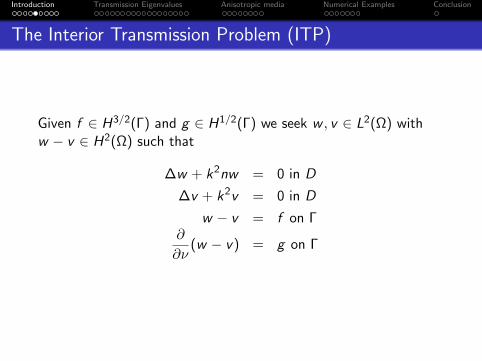
The Interior Transmission Problem (ITP)
Given f ∈ H3/2(Γ) and g ∈ H1/2(Γ) we seek w , v ∈ L2(Ω) withw − v ∈ H2(Ω) such that
∆w + k2nw = 0 in D
∆v + k2v = 0 in D
w − v = f on Γ∂
∂ν(w − v) = g on Γ

Introduction Transmission Eigenvalues Anisotropic media Numerical Examples Conclusion
Study of the ITP
Study of the existence and continuous dependence of solutions ofthe ITP are part of the analysis of the “Linear Sampling Method”for inverse scattering.For such studies see
Colton, Coyle and Monk, SIAM Review (2000)
Qualitative Methods in Inverse Scattering Theory, Colton &Cakoni (2006)
In the cases studied so far (including Maxwell!) the ITP has aunique solution for suitable data and a sufficiently regular domain,except possibly at a countable discrete set of TransmissionEigenvalues that we shall define shortly.

Introduction Transmission Eigenvalues Anisotropic media Numerical Examples Conclusion
ITP and Metamaterials
Consider a simple boundary value problem for ∇ · A∇u + k2nu = 0for negative refractive index materials. Suppose D = D1 ∪ D2 andD1 and D1 meet at an edge Σ. Then if A = 1 and n = 1 in domain1 and A = −a2I , a2 > 0 and n = −n2, n2 > 0 in domain 2 thesolution of the solution u1 in domain D1 and u2 in D2 satisfies
∆u1 + k2u1 = f1 in D1
∆u2 + k2n2/a2u2 = f2 in D2
u1 − u2 = 0 on Σ∂u1
∂ν1− a2
∂u2
∂ν2= 0 on Σ
u = 0 on Γ
where νj is the unit outward normal to Dj .

Introduction Transmission Eigenvalues Anisotropic media Numerical Examples Conclusion
Change of variables for a special domain
Suppose Ω is the symmetric domain shown. Let x = −x . Letu1(x , y) = u1(−x , y), x > 0, etc. Then
x=0
ΩΣ
Γ
Ω1 2
∆u1 + k2u1 = f1 in D2
∆u2 + k2n2/a2u2 = f2 in D2
u1 − u2 = 0 on Σ∂u1
∂ν2− a2
∂u2
∂ν2= 0 on Σ
u = 0 on Γ ∩ ∂D2
On Σ we see the ITP boundary condition.

Introduction Transmission Eigenvalues Anisotropic media Numerical Examples Conclusion
Comments on negative index materials
The observation of the connection of negative index materials andthe ITP is due to Bonnet-BenDhia and Ciarlet Jr. They thenapplied variational methods used in the analysis of the ITP to thenegative index problem and derive well posed variationalformulations:
Bonnet-BenDhia, Ciarlet Jr and Zwolf (2006) - HelmholtzEquation
Bonnet-BenDhia, Ciarlet Jr and Zwolf (2006) - Maxwell
The poster of Chesnel here (requires backwards in time travel)
We shall not pursue this line of research further, but turn insteadto study transmission eigenvalues.

Introduction Transmission Eigenvalues Anisotropic media Numerical Examples Conclusion
Transmission Eigenvalues
Definition: k > 0 is a transmission eigenvalue if there exists anontrivial solution v ∈ L2(D), w ∈ L2(D), v − w ∈ H2
0 (D) of theinterior transmission problem
∆w + k2n(x)w = 0 in D
∆v + k2v = 0 in D
w = v on ∂D∂w
∂ν=
∂v
∂νon ∂D

Introduction Transmission Eigenvalues Anisotropic media Numerical Examples Conclusion
But what are they physically?
The transmission eigenvalues are wave numbers for which thereexists an incident field that generates an arbitrarily small scatteredfield (if v is a Herglotz wave function, the scattered field vanishesprecisely).
Note that the incident field is very special.

Introduction Transmission Eigenvalues Anisotropic media Numerical Examples Conclusion
Transmission Eigenvalues
Theorem
Let m = 1− n and assume |m(x)| > 0 for x ∈ D. Thentransmission eigenvalues exist and form a discrete set whose onlyaccumulation point is infinity.
Proof: Colton-Monk (1988), Paivarinta-Sylvester (2008), Kirsch(2009), Cakoni-Gintides-Haddar (to appear).
Definition: A solution of the Helmholtz equation of the form
vg (x) :=
∫Ω
e ikx ·dg(d)ds(d), g ∈ L2(Ω)
is called a Herglotz wave function with kernel g .

Introduction Transmission Eigenvalues Anisotropic media Numerical Examples Conclusion
Transmission eigenvalues can be measured!
Theorem
Let m = 1− n and assume |m| > 0 for x ∈ D. Let uδ∞(x , d) be the
measured ”noisy” far field pattern with noise parameter δ and forz ∈ D let gz,δ be the Tikhonov regularized solution of the far fieldequation (F δg)(x) = Φ∞(x , z).
If k is not a transmission eigenvalue then limδ→0 ‖vgz,δ‖L2(D)
exists.
If k is a transmission eigenvalue and the far field operator Fhas dense range then for almost every z ∈ D
limδ→0
‖vgz,δ‖L2(D) = ∞.
Proof: Arens (2004), Cakoni-Colton-Haddar (to appear).
Note: ‖vgz,δ‖L2(D) →∞ implies ‖gz,δ‖L2(D) →∞.

Introduction Transmission Eigenvalues Anisotropic media Numerical Examples Conclusion
What do transmission eigenvalues say about n(x)?
Colton-Paivarinta-Sylvester 2007 have proved the followingFaber-Krahn type inequality.
Let k1,n(x) be the first transmission eigenvalue and let λ1(D) bethe first Dirichlet eigenvalue for −∆2 in D.
Theorem
If n(x) > α > 1 for x ∈ D. Then
k21,n(x) ≥
λ1(D)
supDn.

Introduction Transmission Eigenvalues Anisotropic media Numerical Examples Conclusion
A Sharper Faber-Krahn type Inequality
Let n∗ = infD(n) and n∗ = supD(n).
Theorem
If 1 + α ≤ n∗ ≤ n(x) ≤ n∗ < ∞ for x ∈ D then
0 < k1,n∗ ≤ k1,n(x) ≤ k1,n∗ .
Proof: Cakoni-Gintides-Haddar (to appear).
As we shall see, this result allows us to estimate n(x) from interioreigenvalues.

Introduction Transmission Eigenvalues Anisotropic media Numerical Examples Conclusion
Numerical methods for Transmission Eigenvalues
To implement schemes based on the previous theorem, and assessthe accuracy of estimates we need ways to compute transmissioneigenvalues.
In (Colton-Monk-Sun, 2009) we have investigated three waysmotivated by different variational formulations of the ITP. Recallthe eigenvalue problem is to find k and (w , v) 6= 0 such that
∆w + k2n(x)w = 0 in D
∆v + k2v = 0 in D
w = v on ∂D∂w
∂ν=
∂v
∂νon ∂D
Note that k = 0 is an eigenvalue with an infinite dimensionaleigenspace.

Introduction Transmission Eigenvalues Anisotropic media Numerical Examples Conclusion
Method 1: Fourth order problem
Following (Rynne and Sleeman, 1992), assuming n 6= 1, letz = w − v then using the differential equations
∆z + k2n(x)z = −(∆v + k2n(x)v) = k2(1− n(x))v
so we arrive at the problem of finding k and z 6= 0, z ∈ H2(Ω)such that
(∆ + k2)(1− n)−1(∆z + k2n(x)z) = 0 in D
z = 0 and∂z
∂ν= 0 on Γ

Introduction Transmission Eigenvalues Anisotropic media Numerical Examples Conclusion
Method 1 continued
This can be put into the variational problem of finding k andz 6= 0, z ∈ H2
0 (Ω) such that∫D(1− n)−1(∆z + k2n(x)z)(∆ξ + k2ξ) dA = 0 for all ξ ∈ H2
0 (D).
Note:
We can “easily” discretize this problem using Argyriselements.
The problem is now a quadratic eigenvalue probem. Thebilinear form is not Hermitian.
k = 0 is not an eigenvalue.
At the discrete level we can convert back to a generalizedmatrix eigenvalue problem.

Introduction Transmission Eigenvalues Anisotropic media Numerical Examples Conclusion
Method 2: Mixed method
Introducing u = ∇v and rewriting the ITP, we obtain
∆w + k2nw = 0 in D,
u−∇v = 0 in D,
∇ · u + k2v = 0 in D,
w − v = 0 on ∂D,
∂w
∂ν− u · ν = 0 on ∂D.
LetH(div;D) = u ∈ (L2(D))2 | ∇ · u ∈ L2(D).

Introduction Transmission Eigenvalues Anisotropic media Numerical Examples Conclusion
The mixed method continued
The weak formulation for this problem is to find k ∈ C,w ∈ H1(D), u ∈ H(div,D), and v ∈ L2(D) such that∫
D −∇w · ∇φ + k2nwφ dx +∫∂D u · νφ ds = 0, ∀φ ∈ H1(D),∫
D u · τ dx +∫D v∇ · τ dx −
∫∂D τ · νw ds = 0, ∀τ ∈ H(div;D),∫
D ∇ · uq dx + k2∫D vq dx = 0, ∀q ∈ L2(D).
Note:
We can easily discretize this problem using Raviart-Thomaselements.
We can eliminate u to obtain a generalized eigenproblem.
Symmetry is lost between w and v complicating spectrum fork = 0.
Problem of regularity assumed for w .

Introduction Transmission Eigenvalues Anisotropic media Numerical Examples Conclusion
Method 3: Continuous elements
Let H1(D) = H10 (D)⊕ S where S is the H1 orthogonal
complement of H10 (D). Set
w = w0 + wB where w0 ∈ H10 (D) and wB ∈ S ,
v = v0 + wB where v0 ∈ H10 (D).
Note w = v on Γ

Introduction Transmission Eigenvalues Anisotropic media Numerical Examples Conclusion
The continuous element method continued
In the usual way, by integration by parts∫D∇(w0 + wB) · ∇ξ − k2n(w0 + wB)ξ dx = 0 ∀ξ ∈ H1
0 (D)∫Ω∇(v0 + wB) · ∇η − k2(v0 + wB)η dx = 0 ∀η ∈ H1
0 (D).
To obtain one more system of equation, choosing γ ∈ H1(D)∫D∇w · ∇γ − k2nwγ dx −
∫∂D
∂w
∂νγ ds = 0∫
D∇v · ∇γ − k2vγ dx −
∫∂D
∂v
∂νγ ds = 0.
Subtracting these equations we get the final equation to bediscretized.∫
D∇(w − v) · ∇γ dx − k2
∫D(nw − v)γ dx = 0.
Introduction Transmission Eigenvalues Anisotropic media Numerical Examples Conclusion
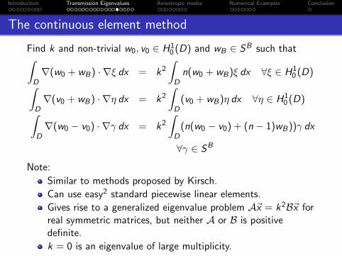
The continuous element method
Find k and non-trivial w0, v0 ∈ H10 (D) and wB ∈ SB such that∫
D∇(w0 + wB) · ∇ξ dx = k2
∫D
n(w0 + wB)ξ dx ∀ξ ∈ H10 (D)∫
D∇(v0 + wB) · ∇η dx = k2
∫D(v0 + wB)η dx ∀η ∈ H1
0 (D)∫D∇(w0 − v0) · ∇γ dx = k2
∫D(n(w0 − v0) + (n − 1)wB))γ dx
∀γ ∈ SB
Note:
Similar to methods proposed by Kirsch.
Can use easy2 standard piecewise linear elements.
Gives rise to a generalized eigenvalue problem A~x = k2B~x forreal symmetric matrices, but neither A or B is positivedefinite.
k = 0 is an eigenvalue of large multiplicity.

Introduction Transmission Eigenvalues Anisotropic media Numerical Examples Conclusion
Numerical results 1: the circle
Table: Transmission eigenvalues of a disk D with radius 1/2. The indexof refraction n is 16. Same mesh for all methods.
Exact 1.9880 2.6129 2.6129 3.2240
Argyris Method 2.0076 (0.98%) 2.6382 2.6396 3.2580
Continuous Method 1.9986 (0.53%) 2.6334 2.6343 3.2641
Mixed Method 1.9912 (0.16%) 2.6218 2.6234 3.2308

Introduction Transmission Eigenvalues Anisotropic media Numerical Examples Conclusion
Numerical Results 2: convergence order
Table: Errors and convergence rates for the first and second transmissioneigenvalues computed by the continuous finite element method. Thedomain D is a disk of radius 1/2. The index of refraction n is 16.khi , i = 1, 2 are the computed first and second eigenvalues on three
meshes.
Mesh size h |kh1 − k1| order |kh
2 − k2| order
h ≈ 0.1 0.04215 - 0.08078 -
h ≈ 0.05 0.01064 1.986 0.02052 1.977
h ≈ 0.025 0.00266 2.002 0.00514 1.995

Introduction Transmission Eigenvalues Anisotropic media Numerical Examples Conclusion
Numerical Results 3: do complex eigenvalues exist?
Table: The first pair of complex transmission eigenvalues of a disk ofradius R = 1/2. The index of refraction n is 16.
Numerical Root Finding Software 4.9009± 0.5781i
Argyris Method 4.9495± 0.5795i
Continuous Method 5.0667± 0.4878i
Mixed Method 4.9350± 0.4959i
It is highly likely that complex eigenvalues exist.

Introduction Transmission Eigenvalues Anisotropic media Numerical Examples Conclusion
Comments on the various methods
Only the Argyris method respects the minimum regularity. Butit is difficult to extend to problems where both A and n vary.
All three methods require to find all eigenvalues (i.e. eig noteigs) and so run out of memory quickly. The Continuousmethod is “cheapest”.
A fourth approach suggested by Cakoni-Gintedes-Haddarinvolving solving a nonlinear equation has also been examinedby Sun.
All methods predict a large number of complex eigenvalues.
We are going to investigate the pseudo-spectrum

Introduction Transmission Eigenvalues Anisotropic media Numerical Examples Conclusion
Scattering by an Anisotropic Medium
u
s
Di
u
∇ · A∇u + k2u = 0 in R2
u = us + ui in R2
limr→∞
√r
(∂us
∂r− ikus
)= 0
where ui (x) = e ikx ·d , |d | = 1 and u ∈ H1loc(R2).
A is a positive, real valued 2× 2 matrix whose entries are piecewisecontinuously differentiable in D and A− I has compact support D.The scattered field us has the asymptotic behavior
us(x) =e ikr
√ru∞(x , d) + O
(r−3/2
)as r →∞ where x = x/|x |, r = |x | and k > 0 is the wave number.u∞(x , d) is the far field pattern of the scattered field us .

Introduction Transmission Eigenvalues Anisotropic media Numerical Examples Conclusion
The Far Field Operator
Let Ω := x : |x | = 1 and define the far field operatorF : L2(Ω) → L2(Ω) by
(Fg)(x) :=
∫Ω
u∞(x , d)g(d)ds(d).
For z ∈ D the far field equation is
(Fg)(x) = Φ∞(x , z), g ∈ L2(Ω)
where
Φ∞(x , z) =e iπ/4
√8πk
e−ikx ·z
is the far field pattern of the fundamental solution
Φ(x , z) := i4H
(1)0 (k|x − z |) .

Introduction Transmission Eigenvalues Anisotropic media Numerical Examples Conclusion
Transmission Eigenvalues
k is a transmission eigenvalue if there exists a nontrivial solutionv ,w ∈ H1(D) of the interior transmission problem
∇ · A∇w + k2w = 0 in D
∆v + k2v = 0 in D
w = v on ∂D∂w
∂νA=
∂ν
∂νon ∂D.
where ∂w∂νA
= ν · A∇w .
Theorem
If ‖A−1‖2 ≥ α > 1 or ‖A−1‖2 ≤ 1− α < 1 then transmissioneigenvalues exist and form a discrete set whose only accumulationpoint is infinity.
Proof: Kirsch (2009), Cakoni-Gintides-Haddar (to appear).

Introduction Transmission Eigenvalues Anisotropic media Numerical Examples Conclusion
Transmission Eigenvalues
Let uδ∞(x , d) be the measured “noisy” far field pattern and for
z ∈ D let gz,δ be the Tikhonov regularized solution of the far fieldequation (F δg)(x) = Φ∞(x , z). Let vg denote the Herglotz wavefunction
vg (x) :=
∫Ω
e ikx ·dg(d)ds(d), g ∈ L2(Ω)
Then [Cakoni-Colton-Haddar (2009)]
If k is not a transmission eigenvalue then limδ→0 ‖vgz,δ‖L2(D)
exists.
If k is a transmission eigenvalue and the far field operator Fhas dense range then for almost every z ∈ D
limδ→0
‖vgz,δ‖L2(D) = ∞
Introduction Transmission Eigenvalues Anisotropic media Numerical Examples Conclusion
What do these transmission eigenvalues say about A(x)?
The far field pattern u∞(x , d) for x , d ∈ Ω does not uniquelydetermine A(x) even if u∞ is known for an interval of values of thewave number k!
However, as we have just seen, the transmission eigenvaluescorresponding to A(x) can be determined from u∞. So they mustcontain information about A.

Introduction Transmission Eigenvalues Anisotropic media Numerical Examples Conclusion
A Faber-Krahn Inequality
Theorem
Assume that ‖A−1‖2 ≥ α > 1 for x ∈ D. Then, if k1 is the firsttransmission eigenvalue and λ1(D) is the first Dirichlet eigenvaluefor −∆2 in D,
k21 ≥
λ1(D)
supD‖A−1‖2.
Proof: Cakoni-Colton-Haddar (2009).
Estimates for ‖A−1‖2 using this inequality are rather crude.Furthermore, if ‖A−1‖2 < 1 for x ∈ D all that is known isk21 ≥ λ1(D).

Introduction Transmission Eigenvalues Anisotropic media Numerical Examples Conclusion
Towards Another Faber-Krahn Inequality
Leta∗(x) := smallest eigenvalue of A−1(x) and
a∗(x) := largest eigenvalue of A−1(x).
Define n∗ := infD(a∗(x)) and n∗ = supD(a∗(x)) and denote byk1,n0 be the first transmission eigenvalue of
∆w + k2n0w = 0 in D
∆v + k2v = 0 in D
w = v on ∂D1
n0
∂w
∂ν=
∂v
∂νon ∂D.

Introduction Transmission Eigenvalues Anisotropic media Numerical Examples Conclusion
Faber-Krahn Inequalities
Theorem
If ‖A−1‖2 > 1 + α for x ∈ D then
0 < k1,n∗ ≤ k1,A(x) ≤ k1,n∗ .
Proof: Cakoni-Gintides-Haddar (to appear).

Introduction Transmission Eigenvalues Anisotropic media Numerical Examples Conclusion
Numerical Examples
Given the first transmission eigenvalue k1,A(x) and the domain Dour aim is to obtain information about A−1(x). From the previoustheorem we have that k1,n0 is a monotonic function of n0 and fromCakoni-Colton-Monk-Sun (to appear) we can show that k1,n0 isalso continuous with respect to n0.
Adjusting n0 so that k1,n0 equals the measured transmissioneigenvalue now gives n0 where n∗ ≤ n0 ≤ n∗ i.e. n0 lies betweenthe infimum of the smallest eigenvalue and the supremum of thelargest eigenvalue of A−1(x).

Introduction Transmission Eigenvalues Anisotropic media Numerical Examples Conclusion
The continuous element method
Let H1(D) = H10 (D)⊕ S where S is the H1 orthogonal
complement of H10 (D). Find non trivial uI ∈ H1(D), uB ∈ S and
uI0 ∈ H1
0 such that u = uI + uB and u0 = uI0 + uB and k such that∫
DA∇(uI + uB) · ξ − k2(uI + uB)ξ dA = 0 for all ξ ∈ H1
0 (Ω)∫D∇(uI
0 + uB) · χ− k2(uI0 + uB)χ d = 0 for all χ ∈ H1
0 (Ω)∫D
A∇(uI + uB) · µ− k2(uI + uB)µ, dA =∫D
A∇(uI0 + uB) · µ− k2(uI
0 + uB)µ dA for all µ ∈ S .
From Cakoni-Colton-Monk-Sun (2009)

Introduction Transmission Eigenvalues Anisotropic media Numerical Examples Conclusion
A test: Eigenvalues for the circle, isotropic media
Set z = 0, plot ‖gz,δ‖L2(Ω) against wave number k.
5 6 7 8 9 10 11 12 13 14 150
5
10
15
20
25
30
Wave number k
No
rm o
f th
e H
erg
lotz
ker
nel
Use
A = Aiso =
(1/4 00 1/4
)Peaks should correspond to realinterior transmission eigenval-ues. Crosses denote computedeigenvalues.
Clearly many eigenvalues are missing from the scan. Why?
Introduction Transmission Eigenvalues Anisotropic media Numerical Examples Conclusion
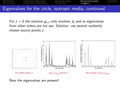
Eigenvalues for the circle, isotropic media, continued
For z = 0 the solution gz,δ only involves J0 and so eigenvaluesfrom other orders are not see. Solution: use several randomlychosen source points z
−1 −0.5 0 0.5 1−1
−0.8
−0.6
−0.4
−0.2
0
0.2
0.4
0.6
0.8
1
5 6 7 8 9 10 11 12 13 14 150
5
10
15
20
25
30
Wave number k
No
rm o
f th
e H
erg
lotz
ker
nel
5 6 7 8 9 10 11 12 13 14 150
5
10
15
20
25
30
Wave number k
Avera
ge n
orm
of
the H
erg
lotz
kern
el
25 random points zi ‖gzi‖
L2(Ω)against k The average of ‖gzi
‖L2(Ω)
Now the eigenvalues are present!

Introduction Transmission Eigenvalues Anisotropic media Numerical Examples Conclusion
Numerical Examples: Homogeneous Anisotropic Media
We consider D to be the unit square [−1/2, 1/2]× [−1/2, 1/2]and
A−11 =
(2 00 8
)A−1
2 =
(6 00 8
)and
A−12r =
(7.4136 −0.9069−0.9069 6.5834
)In each case we can find k1,A from the far field equation, and thencompute n0 that gives the same interior transmission eigenvalue.

Introduction Transmission Eigenvalues Anisotropic media Numerical Examples Conclusion
Computing the first transmission eigenvalue for the square
3 3.5 4 4.5 5 5.5 6 6.5 7 7.5 80
5
10
15
20
25
30
Wave number k
No
rm o
f th
e H
erg
lotz
ker
nel
3 3.5 4 4.5 5 5.5 6 6.5 7 7.5 80
5
10
15
Wave number k
Ave
rag
e n
orm
of
the
Her
glo
tz k
ern
els
25 random points zi ‖gzi‖
L2(Ω)against k The average of ‖gzi
‖L2(Ω)
Computation of the transmission eigenvalues from the far fieldequation for the square D and A−1
2r .

Introduction Transmission Eigenvalues Anisotropic media Numerical Examples Conclusion
Computed values of n0
Domain Matrix E-values (A−1) k1,D,A(x) Predicted n0
Circle Aiso 4,4 5.8 4.03A1 2,8 4.81 5.32A2 6,8 3.95 7.46A2r 6,8 3.95 7.46
Square Aiso 4,4 5.3 4.03A1 2,8 4.1 5.81A2 6,8 3.55 7.41A2r 6,8 3.7 6.90
L shape Aiso 4,4 6.45 4.38A1 2,8 5.2 5.49A2 6,8 4 8A2r 6,8 4.1 7.69
Introduction Transmission Eigenvalues Anisotropic media Numerical Examples Conclusion
Conclusion
The ITP is a novel interior problem which manifests itself inphysical scattering measurements
Interior transmission eigenproblems are currently under studyfor the acoustic, elastic and Maxwell systems
An efficient method for computing the interior transmissioneigenvalues is yet to be developed
Much of this material already extends to Maxwell’s equations