1

arXiv:0806.3738v3 [q-bio.NC] 21 October 2008

The Influence of Sodium and Potassium Dynamics on Excitability,

Seizures, and the Stability of Persistent States: I. Single Neuron

Dynamics.

John R. Cressman Jr.1, Ghanim Ullah

2, Jokubas Ziburkus

3, Steven J. Schiff

2, 4, and Ernest

Barreto1

1 Department of Physics & Astronomy and The Krasnow Institute for Advanced Study,

George Mason University, Fairfax, VA, 22030, USA, 2

Center for Neural Engineering,

Department of Engineering Science and Mechanics, The Pennsylvania State University,

University Park, PA, 16802, USA, 3

Department of Biology and Biochemistry, The

University of Houston, Houston, TX, 77204, USA, and 4 Departments of Neurosurgery

and Physics, The Pennsylvania State University, University Park, PA, 16802, USA.

2

ABSTRACT

In these companion papers, we study how the interrelated dynamics of sodium

and potassium affect the excitability of neurons, the occurrence of seizures, and the

stability of persistent states of activity. In this first paper, we construct a mathematical

model consisting of a single conductance-based neuron together with intra- and

extracellular ion concentration dynamics. We formulate a reduction of this model that

permits a detailed bifurcation analysis, and show that the reduced model is a reasonable

approximation of the full model. We find that competition between intrinsic neuronal

currents, sodium-potassium pumps, glia, and diffusion can produce very slow and large-

amplitude oscillations in ion concentrations similar to what is seen physiologically in

seizures. Using the reduced model, we identify the dynamical mechanisms that give rise

to these phenomena. These models reveal several experimentally testable predictions.

Our work emphasizes the critical role of ion concentration homeostasis in the proper

functioning of neurons, and points to important fundamental processes that may underlie

pathological states such as epilepsy.

Keywords: Potassium dynamics; bifurcation; glia; seizures; instabilities

INTRODUCTION

The Hodgkin-Huxley equations (Hodgkin and Huxley, 1952) have played a vital

role in our theoretical understanding of various behaviors seen in neuronal studies both at

the single-cell and network levels. However, use of these equations often assumes that

the intra- and extra-cellular ion concentrations of sodium and potassium are constant.

While this may be a reasonable assumption for the isolated squid giant axon, its validity

in other cases, especially in the mammalian brain, is subject to debate. In this first of two

companion papers, we investigate the role of local fluctuations in ion concentrations in

modulating the behavior of a single neuron.

Most studies investigating normal brain states have focused primarily on the

intrinsic properties of neurons. Although some studies have examined the role that the

extracellular micro-environment plays in pathological behavior (Bazhenov et al., 2004;

Kager et al., 2000; Somjen, 2004; Park and Durand, 2006, Frohlich et al., 2008), little

3

attention has been paid to the cellular control of micro-environmental factors as a means

to modulate the neuronal response (Park and Durand, 2006).

In general, the intrinsic excitability of neuronal networks depends on the reversal

potentials for various ion species. The reversal potentials in turn depend on the intra- and

extracellular concentrations of the corresponding ions. During neuronal activity, the

extracellular potassium and intracellular sodium concentrations ([K]o and [Na]i,

respectively) increase (Amzica et al., 2002; Heinemann et al., 1977; Moody et al., 1974;

Ransom et al., 2000). Glia help to reestablish the normal ion concentrations, but require

time to do so. Consequently, neuronal excitability is transiently modulated in a competing

fashion: the local increase in [K]o raises the potassium reversal potential, increasing

excitability, while the increase in [Na]i leads to a lower sodium reversal potential and

thus less ability to drive sodium into the cell. The relatively small extracellular space and

weak sodium conductances at normal resting potential can cause the transient changes in

[K]o to have a greater effect over neuronal behavior than the changes in [Na]i, and the

overall increase in excitability can cause spontaneous neuronal activity (Mcbain, 1994;

Rutecki et al., 1985; Traynelis and Dingledine, 1988).

In this paper, we examine the mechanisms by which the interrelated dynamics of

sodium and potassium affect the excitability of neurons and the occurrence of seizure-like

behavior. Since modest increases in [K]o are known to produce more excitable neurons,

we seek to understand ion concentration dynamics as a possible mechanism for giving

rise to and perhaps governing seizure behavior. Using the major mechanisms responsible

for the upkeep of the cellular micro-environment, i.e. pumps, diffusion, glial buffering,

and channels, we mathematically model a conductance-based single neuron embedded

within an extracellular space and glial compartments. We formulate a reduction of this

model that permits a detailed analytical bifurcation analysis of the dynamics exhibited by

this model, and show that the behavior produced by the reduced model is a reasonable

approximation of the full model’s dynamics. The effects of ion concentration dynamics

on the behavior of networks of neurons is addressed in the companion article (Ullah et

al., Submitted).

Some related preliminary results have previously appeared in abstract form

(Cressman et al, 2008).

4

METHODS

1. Full model

Our full model consists of one single-compartment conductance-based neuron

containing sodium, potassium, calcium-gated potassium, and leak currents, augmented

with dynamic variables representing the intracellular sodium and extracellular potassium

concentrations. These ion concentrations are affected by the neuron’s intrinsic ionic

currents as well as a sodium-potassium pump current, a glial current, and potassium

diffusion. Finally, the concentrations are coupled to the membrane voltage equations via

the Nernst reversal potentials.

The conductance-based neuron is modeled as follows:

Na K Cl

dVC I

dtI I

3

( ) ( )Na Na Na NaL NaI g m V h V V g V V

4 [ ]( ) ( )

1 [ ]

AHP iK K K KL K

i

g CaI g n V V g V V

Ca

( )Cl ClL ClI g V V

dq

dt [

q(V )(1 q)

q(V )q], q n,h

d[Ca]i

dt 0.002g

Ca(V V

Ca) / {1 exp((V 25) / 2.5)} [Ca]

i/ 80 (1)

The supporting rate equations are:

m(V ) m (V ) /(m (V ) m (V ))

m (V ) 0.1(V 30) /[1 exp(0.1(V 30))]

m (V ) 4exp((V 55) /18)

n (V ) 0.01(V 34) /[1 exp(0.1(V 34))]

n (V ) 0.125exp((V 44) /80)

h (V ) 0.07exp((V 44) /20)

h (V ) 1/[1 exp(0.1(V 14))]

Note that the overall leak current consists of the final terms in the above

expressions for NaI and KI , plus ClI ; similar leak currents were used by (Kager et al.,

5

2000). Also, the gating variable m is assumed to be fast compared to the voltage change;

we therefore assume it reaches its equilibrium value m immediately (Rinzel, 1985;

Pinsky and Rinzel, 1994). Finally, the active internal calcium concentration is used only

in conjunction with the calcium-gated potassium current in order to model the adaptation

seen in many excitatory cells (Mason and Larkman, 1990; Wang, 1998).

The meaning and values of the parameters and variables used in this paper are

given in Table 1.

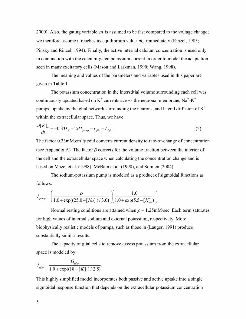
The potassium concentration in the interstitial volume surrounding each cell was

continuously updated based on K+ currents across the neuronal membrane, Na

+-K

+

pumps, uptake by the glial network surrounding the neurons, and lateral diffusion of K+

within the extracellular space. Thus, we have

[ ]0.33 2 .o

K pump glia diff

d KI I I I

dt (2)

The factor 0.33mM.cm2/coul converts current density to rate-of-change of concentration

(see Appendix A). The factor corrects for the volume fraction between the interior of

the cell and the extracellular space when calculating the concentration change and is

based on Mazel et al. (1998), McBain et al. (1990), and Somjen (2004).

The sodium-potassium pump is modeled as a product of sigmoidal functions as

follows:

1.0.

1.0 exp((25.0 [ ] ) / 3.0) 1.0 exp(5.5 [ ] )pump

i o

INa K

Normal resting conditions are attained when = 1.25mM/sec. Each term saturates

for high values of internal sodium and external potassium, respectively. More

biophysically realistic models of pumps, such as those in (Lauger, 1991) produce

substantially similar results.

The capacity of glial cells to remove excess potassium from the extracellular

space is modeled by

Iglia

G

glia

1.0 exp((18 [K]o) / 2.5)

.

This highly simplified model incorporates both passive and active uptake into a single

sigmoidal response function that depends on the extracellular potassium concentration

6

alone. Normal conditions correspond to Gglia = 66mM/sec, and [K]o = 4.0mM. A similar

but more biophysical approach was used in (Kager et al., 2000). Two factors allow the

glia to provide a nearly insatiable buffer for the extracellular space. The first is the very

large size of the glial network. Second, the glial endfeet surround the pericapillary space,

which, through interactions with arteriole walls, can effect blood flow; this, in turn, can

increase the buffering capability of the glia (Paulson and Newman, 1987, Kuschinsky et

al., 1972, McCulloch et al., 1982).

The diffusion of potassium away from the local extracellular micro-environment

is modeled by

I

diff ([K]

o k

o,).

Here, k

o, is the concentration of potassium in the largest nearby reservoir.

Physiologically, this would correspond to either the bath solution in a slice preparation,

or the vasculature in the intact brain (noting that [K]o is kept below the plasma level by

trans-endothelial transport). For normal conditions, we use k

o,= 4.0 mM. The diffusion

constant , obtained from Fick’s law, is 2D / x2, where we use D = 2.510-

6cm

2/sec for K

+ in water (Fisher et al., 1976) and estimate x 20m for intact brain

reflecting the average distance between capillaries (Scharrer, 1944); thus = 1.2Hz.

To complete the description of the potassium concentration dynamics, we make

the assumption that the flow of Na+ into the cell is compensated by flow of K

+ out of the

cell. Then [K]i can be approximated by

[ ] 140.0 (18.0 [ ] ),i iK mM mM Na (3) where

140.0 mM and 18.0 mM reflect the normal resting [K]i and [Na] i respectively. The

limitations of this approximation will be addressed in the discussion section.

The intra- and extracellular sodium concentration dynamics are modeled by

d[Na]i

dt 0.33

INa

3I

pump (4)

[ ] 144.0 ([ ] 18.0 ).o iNa mM Na mM (5)

7

In equation (5), we assume that the total amount of sodium is conserved, and hence only

one differential equation for sodium is needed. Here, 144.0mM is the sodium

concentration outside the cell under normal resting conditions for a mammalian neuron.

Finally, the reversal potentials appearing in equation (1) are obtained from the ion

concentrations via the Nernst equation

[ ]26.64ln

[ ]

ONa

i

NaV

Na

[ ]26.64ln

[ ]

OK

i

KV

K

[ ]26.64ln .

[ ]

iCl

o

ClV

Cl

With the leak conductances listed above, the chloride concentrations were fixed at

[ ]iCl =6.0mM and [ ]oCl =130mM.

Thus, the dynamic variables of the full model are V, n, h, [Ca]

i, [ ]oK , and [ ]iNa .

Despite the fact that we have neglected many features of real mammalian cells (such as

the geometrically complex dendritic and axonal structure and the related spatially

complex distribution of channels and cotransporters, as well as the presence of immobile

anions which are strictly required to maintain electric and osmotic balance), our model

captures the essential dynamics that we wish to explore.

In the results section, we will be interested in varying the parameters gliaG , ,

k

o,, and . We will present our results in terms of parameters normalized by their

normal values, for example, ,/glia glia glia normalG G G , where the overbar indicates the

normalized parameter.

2. Reduced model

In order to more effectively study the bifurcation structure of the model presented

above, we formulated a reduction by eliminating the fast-time-scale spiking behavior in

favor of the slower ion concentration dynamics. This is accomplished by replacing the

entire Hodgkin-Huxley mechanism with empirical fits to time-averaged ion currents.

8

Using the membrane conductances from the full model, we fixed the internal and external

sodium and potassium concentration ratios and allowed the model cell to attain its

asymptotic dynamical state, which was either a resting state or a spiking state. Then, the

sodium and potassium membrane currents were time-averaged over one second. These

data were fit to products of sigmoidal functions of the sodium and potassium

concentration ratios, resulting in the (infinite-time) functions

I

Na[Na]

i/ [Na]

o,[K]

o/ [K]

i and I

K[Na]

i/ [Na]

o,[K ]

o/ [K ]

i . Details are available

in Appendix A. NaI

is nearly identical toKI

, differing significantly only near normal

resting concentration ratios due to differences in the sodium and potassium leak currents.

Thus, our reduced model consists of equations (2-5), with NaI and

KI replaced

with the empirical fits described above (see Appendix A for additional details).

3. Bifurcations in the reduced model

Our main results in this paper consist of identifying bifurcations in the reduced

model and analyzing their implications for the behavior of the full model. We observe

that depending on the various parameters, the ion concentrations in the reduced model

approach either stable equilibria, and thus remain constant, or they approach stable

periodic orbits, and thus exhibit oscillatory behavior (Fig 1). As parameters are changed,

the stability of these solutions change. This happens through bifurcations (a good general

reference is Strogatz (1994)). Most relevant for our purposes are the Hopf bifurcation,

and the saddle-node bifurcation of periodic orbits. In a Hopf bifurcation, an equilibrium

solution either gains or loses stability, and simultaneously, a periodic orbit either appears

or disappears from the same point1. In a saddle-node bifurcation of periodic orbits, a pair

of periodic orbits – one stable and one unstable – either appears or disappears suddenly,

as if out of “thin air”.

Bifurcation diagrams were obtained using XPPAUT (Ermentrout, 2002). Code for

both of our models is available from ModelDB.2

1 Depending on the stabilities of the equilibrium and the periodic orbit involved, Hopf bifurcations are

classified as sub- or supercritical. 2 http://senselab.med.yale.edu/modeldb/

9

RESULTS

1. Overview

In an experimental slice preparation, an easily-performed experimental

manipulation is to change the potassium concentration in the bathing solution. Such

preparations have been used to study epilepsy (Jensen and Yaari, 1997; Traynelis and

Dingledine, 1988; Gluckman, et al. 2001). At normal concentrations (~4mM), normal

resting potential is maintained. However, at higher concentrations (8mM, for example)

bursts and seizure-like events occur spontaneously.

We begin discussing the dynamics of our models by considering a similar

manipulation, corresponding to varying the normalized parameter k

o,. In the full model,

setting k

o,= 2.0 (i.e., doubling the normal concentration of potassium in the bath

solution) leads to spontaneously-occurring prolonged periods of rapid firing, as illustrated

in the top trace of Fig. 1. These oscillations are remarkably similar to experimental results

reported by several investigators (see, for example, Figures 1 and 6 of Jensen and Yaari

(1997), in which the authors use a high potassium in vitro preparation, and Figure 2 of

Ziburkus et al. (2006), which reports results from a 4-aminopyridine in vitro preparation).

Each event lasts on the order of tens of seconds and consists of many spikes, each of

which occurs on the order of 1 ms. Thus, the full model contains dynamics on at least two

distinct time scales that are separated by four orders of magnitude: fast spiking from the

Hodgkin-Huxley mechanism, and a slow overall modulation. The solid traces in the

middle and bottom panels show that this slow modulation corresponds to slow periodic

behavior in the sodium and potassium ion concentrations, respectively.

Our reduced model was constructed in order to remove the fast Hodgkin-Huxley

spiking mechanism and focus attention on the slow dynamics of the ion concentrations.

The dashed traces in the middle and bottom panels of Fig. 1 show the sodium and

potassium ion concentrations obtained from the reduced model for the same parameters

used above. Although these traces are not identical to those of the full model, it is evident

that the reduced model captures the qualitative behavior of the ion concentrations quite

well.

10

The separation of time scales achieved by our model reduction (see, for example,

Rinzel and Ermentrout (1989); Kepler, et al., (1992)) yields a model that is amenable to

numerical bifurcation analysis. Knowledge of the bifurcation structure in turn informs us

about the dynamical mechanisms that underlie the full model. In the following, we will

first describe the main dynamical features of the reduced model, and then examine the

implications for the behavior of the full model.

2. Analysis of the reduced model

Fig. 2 shows a bifurcation diagram obtained using the reduced model. This

diagram plots the minimum and maximum asymptotic values of the extracellular

potassium concentration [ ]oK versus a range of values of the reservoir’s normalized

potassium concentration k

o,. For low values of this parameter, [ ]oK is observed to settle

at a stable equilibrium. The value of [ ]oK corresponding to this equilibrium increases

with k

o, until the equilibrium loses stability via a subcritical Hopf bifurcation at

k

o,1.9 . This means that at this point, an unstable periodic orbit collapses onto the

equilibrium, and both disappear. [ ]oK is subsequently attracted to a coexisting large-

amplitude stable periodic orbit3. Thus, large-amplitude oscillations in [ ]oK appear

abruptly. These oscillations persist as k

o, is increased until the same sequence of

bifurcations occurs in the opposite order at k

o, 2.13. At this higher value of

k

o,, the

unstable equilibrium undergoes a subcritical Hopf bifurcation, becoming stable and

giving rise to an unstable periodic orbit whose amplitude quickly rises with increasing

k

o,. This orbit then collides with the large-amplitude stable periodic orbit at

k

o, 2.15,

and both orbits disappear in a saddle-node bifurcation of periodic orbits. In this manner,

3 The stable and unstable periodic orbits involved in this scenario appear via a saddle-node bifurcation at a

slightly smaller parameter value that is extremely close to that of the Hopf bifurcation. Thus, the sequence

of bifurcations is not immediately apparent in Fig. 2. The abruptness of these transitions, and the difficulty

in resolving them numerically, is due to the “canard” mechanism (Dumortier and Roussarie, 1996;

Wechselberger, (2007)).

11

the periodic behavior of [ ]oK is terminated. For still higher values of k

o,, [ ]oK

approaches the equilibrium values shown at the far right in Fig. 2.

In order to examine the boundaries of the oscillatory behavior described above

with respect to pump strength , the diffusion coefficient , and glial buffering strength

gliaG , we constructed the bifurcation diagrams shown in Fig. 3. First, we fixed all

parameters at their normal resting values except k

o,, which we set to 2 in order to obtain

the oscillatory behavior discussed above. We then separately varied , , and gliaG

away from their normal resting values. If and are increased from their nominal

values of 1 (Fig. 3a, b), we see that the oscillatory behavior terminates in a manner

similar to that described above; that is, an unstable periodic orbit appears via a subcritical

Hopf bifurcation which grows until it collides with and annihilates the stable periodic

solution at a saddle-node bifurcation of periodic orbits. (This is most apparent in Fig

3(a).) The same scenario applies as these parameters are decreased4,5. The situation is

similar for the glial strengthgliaG , except that on the left, we see no saddle-node

bifurcation of periodic orbits for positive values of gliaG (Fig. 3c).

It is notable that if or gliaG are reduced from their normal values, larger

amplitude oscillations in [ ]oK occur. This is because, in both cases, the trafficking of

potassium away from the extracellular space is impeded, and consequently, [ ]oK builds

up more effectively during the spiking phase of the cell’s activity (see Fig. 6, below). In

contrast, changing in either direction results in very little change in the amplitude of

the [ ]oK oscillations. Furthermore, the bistable region on the right side of the diagram

is quite wide, and hence hysteretic behavior as is varied across this region may be

particularly amenable to experimental observation (e.g. with ouabain). Finally, we note

that the right branch of stable equilibria in Fig. 3(a) corresponds to higher values of

[ ]oK than the left branch. This is because the cell is active – either spiking or in

4 A canard similar to that described previously occurs here, so that the Hopf and the saddle-node

bifurcations on the left sides of Figs. 3 (a) and (b) occur in extremely narrow intervals of the parameter. 5 In Fig. 3 (a), the equilibrium curve does not extend all the way to zero because of the constant chloride

leak current.

12

depolarization block – and thus there is a large membrane potassium current flowing into

the extracellular space which must be balanced by pumps and otherwise “normal”

diffusion and glial currents.

The two-parameter bifurcation diagram shown in Fig. 4 provides a more complete

understanding of the oscillatory behavior of [ ]oK in our reduced model with respect to

the variation of both and gliaG , with

k

o,= 2. The dashed lines at

gliaG = 1 and = 1

correspond to the one-dimensional bifurcation diagrams shown in Figs. 3b and c. The

solid curves represent Hopf bifurcations, and the intersection of these dashed lines with

the Hopf curves correspond to the Hopf bifurcations (points) in the earlier figures. Thus,

the Hopf curves define a region within which [ ]oK is obliged to oscillate, because the

only stable attractor is a periodic orbit. To facilitate discussion, we refer to this region as

the “region of oscillation”, or RO. Outside of the RO, stable equilibrium solutions for

[K]o exist6.

The dashed line at gliaG = 1.75 corresponds to the one-dimensional bifurcation

diagram shown in Fig. 5. This is drawn at the same scale as Fig. 3b (the gliaG = 1

diagram) to facilitate comparison. We note that the amplitude of the oscillation in [K]o is

significantly smaller in this region of the RO. Furthermore, the Hopf bifurcation on the

right (at about = 3.2) is now supercritical. This means that the amplitude of the [K]o

oscillation decays smoothly to zero as this point is approached from the left.

3. Analysis of the full model

We now investigate whether the dynamical features identified above in our

reduced model correspond to similar features in our full model. Fig. 6 shows traces of the

membrane voltage (upper traces), [K]o (solid lower traces), and [ ]iNa (dashed lower

traces) versus time, all obtained from the full model, corresponding to the parameter

values marked by the numbered squares in Fig. 4. For the regions outside of the RO, the

reduced model predicts stable equilibrium solutions for the ion concentrations. For

example, at point 1, [K]o is slightly elevated at a value near 6mM, and the membrane

6 Note that oscillations may persist slightly outside of the RO, where a stable periodic orbit coexists with

the stable equilibrium solution; see, for example, the right side of Fig. 3(a).

13

voltage of the full model remains constant at -62 mV (not shown). However, at point 2,

the full model exhibits tonic firing, as shown in Fig. 6a. Here, [K]o is sufficiently high

such that the neuron is depolarized beyond its firing threshold, and [K]o remains

essentially constant with only small perturbations of order 0.1 mM due to individual

spikes (Fig. 6a, lower panel) (Frankenhaeuser and Hodgkin, 1956). (These spike

perturbations disappear in the reduced model, as they are smoothed-out by the averaging

in our model reduction procedure.)

Within the RO, the reduced model predicts periodic behavior with relatively large

and slow oscillations in the ion concentrations. Points 3-7 in Fig. 4 correspond to Figs. 6

(b-f), which show various bursting behaviors of the full model. To facilitate comparison,

the time scale for these figures (Fig. 6 b-f) is the same, showing 100 seconds of data. In

addition, the voltage and concentration scales are also the same, except for the

concentration scale in (b). We make the following observations from Fig. 6. As the RO is

traversed from low to high (keeping gliaG fixed) in Fig. 4, the bursts become more

frequent (compare Fig. 6c, d; points 4, 5 and Fig.6e, f; points 6, 7). In addition, the shape

of the burst envelope changes due to the decreasing amplitude of the [K]o oscillations.

Note also in Fig. 6b (point 3) that the peak of the [K]o concentration is nearly 40mM,

large enough to cause the neuron to briefly enter a state of quiescence known as

“depolarization block” (see companion paper, Ullah, et al., Submitted). Finally, the

within-burst spike frequency is essentially constant in Figs. 6 (b)-(f); it does peak in

concert with the peak of [ ]oK , however, this effect is weak.

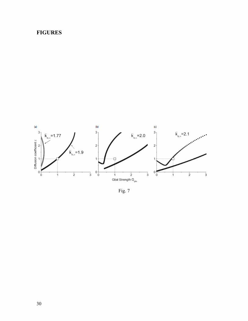
Returning briefly to the reduced model, we address in Fig. 7 how the location of

the RO changes with k

o, as all other parameters are kept at their normal values. As

k

o,

is increased from its normal value at 1, the RO emerges around a value of k

o, 1.77 , as

represented by the gray line on the left of Fig.7a. (This observation is consistent with

Rutecki , et al. (1985)). As k

o, increases, the right edge of the RO shifts towards the

right, crossing the normal values of and gliaG at (1,1) when

k

o,= 1.9, as shown by the

thick solid line in Fig.7a. As k

o, is further increased to 2.0, normal conditions for glial

pumping and diffusion are well inside the RO as shown in Fig. 7b, and correspondingly,

14

we observe bursting/seizing behavior in the full model. Fig. 7c shows the RO when the

reservoir concentration has been increased to 2.1. Here the left side edge of the RO is

just about to cross the point (1,1), after which the ion concentrations assume stable

equilibrium values in the reduced model. Note that these stable equilibria actually

correspond to a state of rapid tonic firing in the full model, as in Fig. 6(a); for much

higher values of k

o, (greater than approximately 7.2mM), [K]o remains constant in the

reduced model, but the full model eventually gives rise to depolarization block.

We conclude by reporting other kinds of bursting behaviors seen in our full

model. Fig. 8a shows a time trace of the membrane voltage for k

o, 6 , 0.1gliaG and

0.4 . These bursts are fundamentally different from those shown in Fig. 6. In

particular, the extracellular potassium concentration is quite elevated, and thus the

periods of quiescence correspond not to resting behavior, but rather to a state of

depolarization block. In addition, the bursts themselves have a rounded envelope, as

opposed to the (approximately) square envelopes of the events shown in Fig. 6. This

behavior is consistent with the experimental observations of (Ziburkus et al., 2006), in

which interneurons were seen to enter depolarization block and thus give way to

pyramidal cell bursts. Bikson et al. also observed depolarization block in pyramidal cells

during electrographic seizures (see Figure 1d from Bikson et al., 2003). We have also

experimentally observed (in oriens interneurons exposed to 4-aminopyridine) relatively

continuous “burst” firing without any quiescent intervals, as seen in Fig.8b. In this figure,

the neuron fires continuously, but with a wavy envelope due to the oscillating ion

concentrations. We include these patterns to complete the description of the repertoire of

single cell bursting behaviors seen in our models.

DISCUSSION

We have created a model which can be used to investigate the role of ion

concentration dynamics in neuronal function, as well as a reduced model which is

amenable to bifurcation analysis. Such bifurcations indicate major qualitative changes in

system behavior, which are in many ways more predictive and informative than purely

quantitative measurements. In particular, we show that under otherwise normal

15

conditions, there exists a broad range of bath potassium concentration values which

yields seizure-like behavior in a single neuron that is both qualitatively as well as

quantitatively similar to what is seen in experimental models (Ziburkus et al., 2006; Feng

and Durand, 2006; McBain, 1994). In fact, the values of extracellular concentration used

in those experiments are quantitatively consistent with the range of concentrations shown

here to exhibit seizures. Furthermore, the stable periodic oscillations in the extracellular

potassium concentration which result from varying various experimentally and

biophysically relevant parameters suggests that these effects may be an important

mechanism underlying epileptic seizures.

In formulating our models, we made several approximations. The two most

severe, insatiable glial buffering and the assumption that internal potassium can be

calculated using equation (3), should hold for times that are long compared to the time

scale of individual spikes, bursts, and seizures. However, for even longer times (on the

order of thousands of seconds), the saturation of glia as well as the decoupling of the

internal potassium from the sodium dynamics will lead to more substantial errors in the

calculated results. It is possible that glia do not fully saturate, if, as suggested by Paulson

and Newman et al (1987), the glia siphon excess potassium into pericapillary spaces via

the astrocyte network. Nevertheless, one can understand a slow partial saturation of the

glial network as a slow decrease in gliaG , for example. Consequently, the system may

enter or leave parameter-space regions in which oscillating ion concentrations exist (e.g.,

see Figs. 3(c) and 4). This long-term behavior could be used to more accurately model

the temporal dynamics of the glial siphoning system.

It is important to note the limitations of our models with respect to extremely long

time scales. If the reservoir concentration k

o, remains only slightly elevated for a long

period of time the model cell will ultimately reach a new fixed point in [K]o nearly equal

to the bath concentration. A stable resting state should exhibit some degree of robustness

in its micro-environment. However, as the system drifts further from the normal state, we

should not expect such homeostasis to persist; the internal potassium will in general drift

to higher or lower values depending on the wide variety of pumps, cotransporters, or

channels inherent to the cell. When the internal potassium is integrated separately (not

16

shown here), we see both upward and downward drift depending on model parameters as

well as the initial conditions for the ionic concentrations. Therefore in our model the

seizure-like events, as well as the tonic firing reported here, appear to be transients on

extremely long time scales. Of course, such phenomena are also transients on long time

scales in animals and humans.

Although our reduced model does a good job reproducing the qualitative results

of our full spiking model, there are regions were the two models disagree. These two

models produce very good agreement in the region of the two-parameter graph presented

in Figure 4. However the reduced model predicts the cessation of all oscillations as gliaG

is increased past a value of 4 (not shown), whereas the full model exhibits burst-like

oscillations for far greater values. This discrepancy is due to the use of relatively simple

functions used in our fitting of the time-averaged Hodgkin-Huxley currents (see

Appendix A). A more sophisticated fit of these data would improve the agreement

between our two models.

Our work points out the important role that ion concentration dynamics may play

in understanding neuronal dynamics, including pathological dynamics such as seizures.

Of course, in realistic situations, these are due to a combination of local environmental

conditions and electrical and chemical communication between cells (see the

accompanying paper, Ullah, et al., Submitted). The models presented here, however,

demonstrate that recurring seizure-like events can occur in a single cell that is subject to

intra- and extracellular ion concentration dynamics (see also discussion in (Kager, et al.,

2000, Kager, et al., 2007) regarding single-cell seizure dynamics). In addition, we have

identified the basic mechanism that can give rise to such events: Hopf bifurcations that

lead to slow oscillations in the ion concentrations.

ACKNOWLEDGEMENTS

This work was funded by NIH Grants K02MH01493 (SJS), R01MH50006 (SJS, GU),

F32NS051072 (JRC), and CRCNS-R01MH079502 (EB).

17

REFERENCES

Amzica, F., Massimini, M., & Manfridi, A. (2002). A spatial buffering during slow and

paroxysmal sleep oscillations in cortical networks of glial cells in vivo. J.

Neurosci. 22:1042–1053.

Bazhenov M, Timofeev I, Steriade M., & Sejnowski T. J. (2004). Potassium model for

slow (2-3 Hz) in vivo neocortical paroxysmal oscillations. J. Neurophysiol. 92:

1116-1132.

Bikson, M., Hahn, P. J., Fox, J. E., & Jefferys, J. G. R. (2003). Depolarization block of

neurons during maintenance of electrographic seizures. J. Neurophysiol.

90(4);2402-2408.

Cressman JR, Ullah G, Ziburkus J, Schiff, SJ, and Barreto E (2008), Ion concentration

dynamics: mechanisms for bursting and seizing. BMC Neuroscience 9 (Suppl

1):O9.

Dumortier, F. & Roussarie, R. (1996). Canard cycles and center manifolds. Memoirs Am.

Math. Soci. 121(577).

Ermentrout, G.B. (2002) Simulating, Analyzing, and Animating Dynamical Systems: A

Guide to XPPAUT for Researchers and Students, Philadelphia: Society for Industrial and

Applied Mathematics.

Feng, Z., & Durand, D. M. (2006). Effects of potassium concentration on firing patterns

of low-calcium epileptiform activity in anesthetized rat hippocampus: inducing of

persistent spike activity. Epilepsia. 47(4):727-736.

Fisher, R. S., Pedley, T. A., & Prince, D. A. (1976). Kinetics of potassium movement in

norman cortex. Brain Res. 101(2):223-37.

Frankenhaeuser, B., & Hodgkin, A.L. (1956). The after-effects of impulses in the giant

nerve fibers of loligo. J. Physiol. 131:341-376.

F. Frohlich, I. Timofeev, T.J. Sejnowski and M. Bazhenov (2008) Extracellular

potassium dynamics and epileptogenesis. In: Computational Neuroscience in

Epilepsy, Editors: Ivan Soltesz and Kevin Staley, p. 419.

Gluckman B.J., Nguyen, H., Weinstein, S.L., & Schiff, S.J. (2001). Adaptive electric

field control of epileptic seizures. J. Neurosci. 21(2):590-600.

Heinemann, U., Lux, H. D., & Gutnick, M. J. (1977). Extracellular free calcium and

potassium during paroxsmal activity in the cerebral cortex of the cat. Exp Brain

Res 27:237–243.

Hodgkin, A. L., & Huxley, A. F. (1952). A quantitative description of membrane current

and its application to conduction and excitation in nerve. J. Physiol. 117:500-544.

Jensen, M.S., & Yaari, Y. (1997). Role of intrinsic burs firing, potassium accumulation,

and electrical coupling in the elevated potassium model of hippocampla epilepsy.

J. Neurophysiol. 77:1224-1233.

Lauger P. (1991). Electrogenic ion pumps. Sunderland, MA: Sinauer.

Kager H, Wadman W. J., & Somjen G. G. (2000). Simulated seizures and spreading

depression in a neuron model incorporating interstitial space and ion

concentrations. J. Neurophysiol. 84: 495-512.

Kager H, Wadman W.J., & Somjen G. G. (2007). Seizure-like afterdischarges simulated

in a model neuron. J. Comput Neurosci. 22: 105-108.

Kepler T.B., Abbott, L.F., & Mardner, E. (1992). Reduction of conductance-based

18

neuron models. Biol. Cybern. 66:381-387.

Mason, A., & Larkman, A. (1990). Correlations between morphology and

electrophysiology of pyramidal neurons in slices of rat visual cortex. II.

Electrophysiology. J. Neurosci. 10(5):1415-1428.

Mazel, T., Simonova, Z. and Sykova, E. (1998). Diffusion heterogeneity and anisotropy

in rat hippocampus. Neuroreport. 9(7):1299-1304.

McBain, C. J., Traynelis, S. F., and Dingledine, R. (1990). Regional variation of

extracellular space in the hippocampus. Science. 249(4969):674-677.

McBain, C.J. (1994). Hippocampal inhibitory neuron activity in the elevated potassium

model of epilepsy. J. Neurophysiol. 72:2853-2863.

Moody, W. J., Futamachi, K. J., & Prince, D. A. (1974). Extracellular potassium activity

during epileptogenesis. Exp. Neurol. 42:248–263.

Park, E. & Durand, D.M. (2006). Role of potassium lateral diffusion in non-synaptic

epilepsy: A computational study. J. Theor. Biol. 238:666-682.

Paulson, O.B. and Newman, E.A. (1987) Does the release of potassium from astrocyte

endfeet regulate cerebral blood flow? Science 237 (4817): 896-898.

Pinsky, P.F. and Rinzel, J. (1994). Intrinsic and network rhythmogenesis in a reduced

Traub model for CA3 neurons. J. Comp. Neurosci. 1:39-60.

Ransom, C. B., Ransom, B. R., & Sotheimer, H. (2000). Activity-dependent

extracellular K+ accumulation in rat optic nerve: the role of glial and axonal Na

+

pumps. J. Physiol. 522:427-442.

Rinzel, J. (1985). Excitation dynamics: insights from simplified membrane models. Fed.

Proc. 44:2944-2946.

Rinzel, J., & Ermentrout, B. (1989). Analysis of neuronal excitability and oscillations,

in “Methods in neuronal modeling: From synapses to networks”, Koch, C., &

Segev, I. MIT Press, revised (1998).

Rutecki, P. A., Lebeda, F. J., & Johnston, D. (1985). Epileptiform activity induced by

changes in extracellular potassium in hippocampus. J. Neurophysiol. 54:1363–

1374.

Scharrer, E. (1944). The blood vessels of the nervous tissue. Quart. Rev. Biol. 19(4):308-

318.

Strogatz, S.H. (1994). Nonlinear Dynamics and Chaos, Addison-Wesley, Reading, MA.

Somjen, G. G. (2004). Ions in the Brain, Oxford University Press, New York.

Traynelis, S. F., & Dingledine, R. (1988). Potassium-induced spontaneous electrographic

seizures in the rat hippocampal slice. J. Neurophysiol. 59:259–276

Wang, X. J. (1999). Synaptic basis of cortical persistent activity: the importance of

NMDA receptors to working memory. J. Neurosci. 19(21):9587-9603.

Wechselberger, M. (2007), Scholarpedia, 2(4):1356.

Ziburkus, J., Cressman, J. R., Barreto, E., & Schiff, S. J. (2006). Interneuron and

pyramidal cell interplay during in vitro seizure-like events. J. Neurophysiol.

95:3948-3954.

19

FIGURE LEGENDS

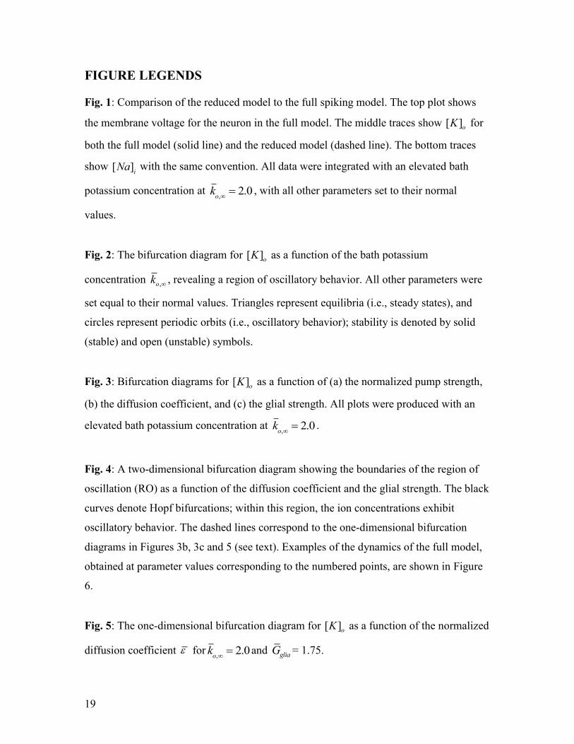
Fig. 1: Comparison of the reduced model to the full spiking model. The top plot shows

the membrane voltage for the neuron in the full model. The middle traces show [ ]oK for

both the full model (solid line) and the reduced model (dashed line). The bottom traces

show [Na]

i with the same convention. All data were integrated with an elevated bath

potassium concentration at k

o, 2.0 , with all other parameters set to their normal

values.

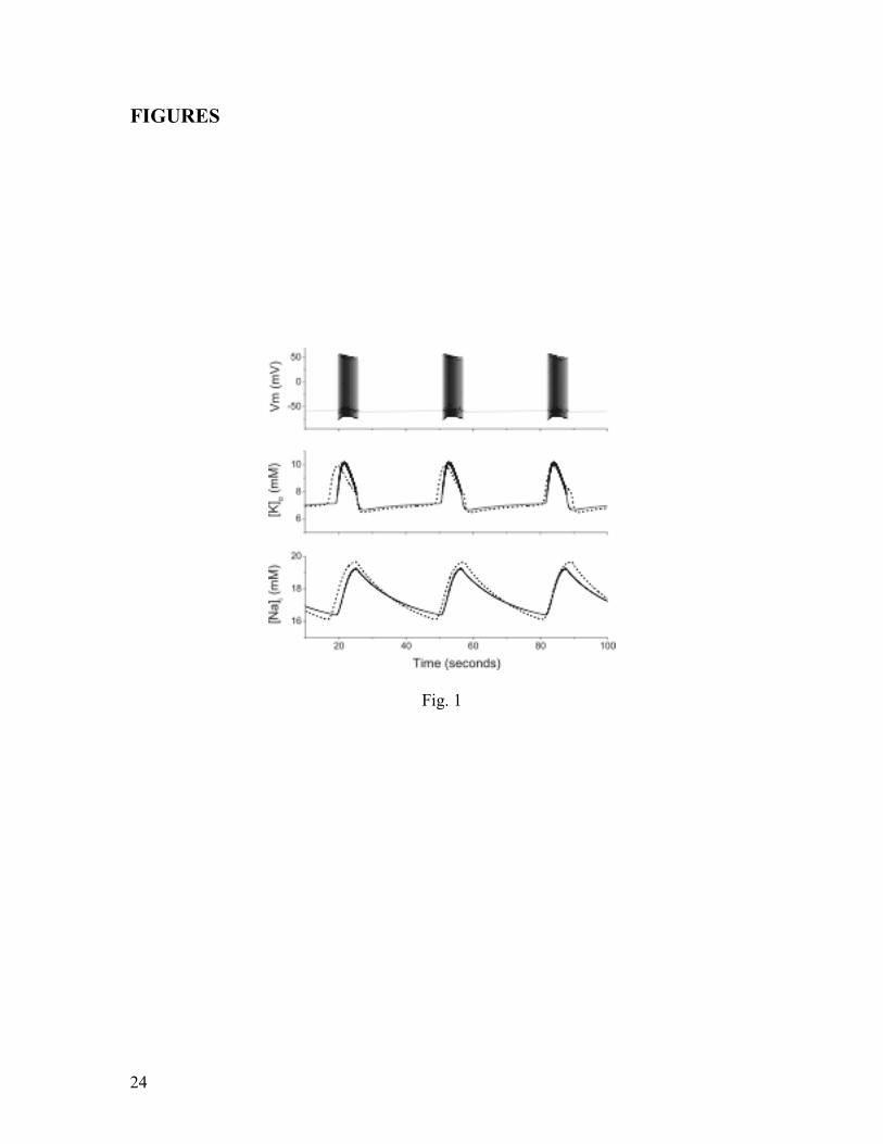
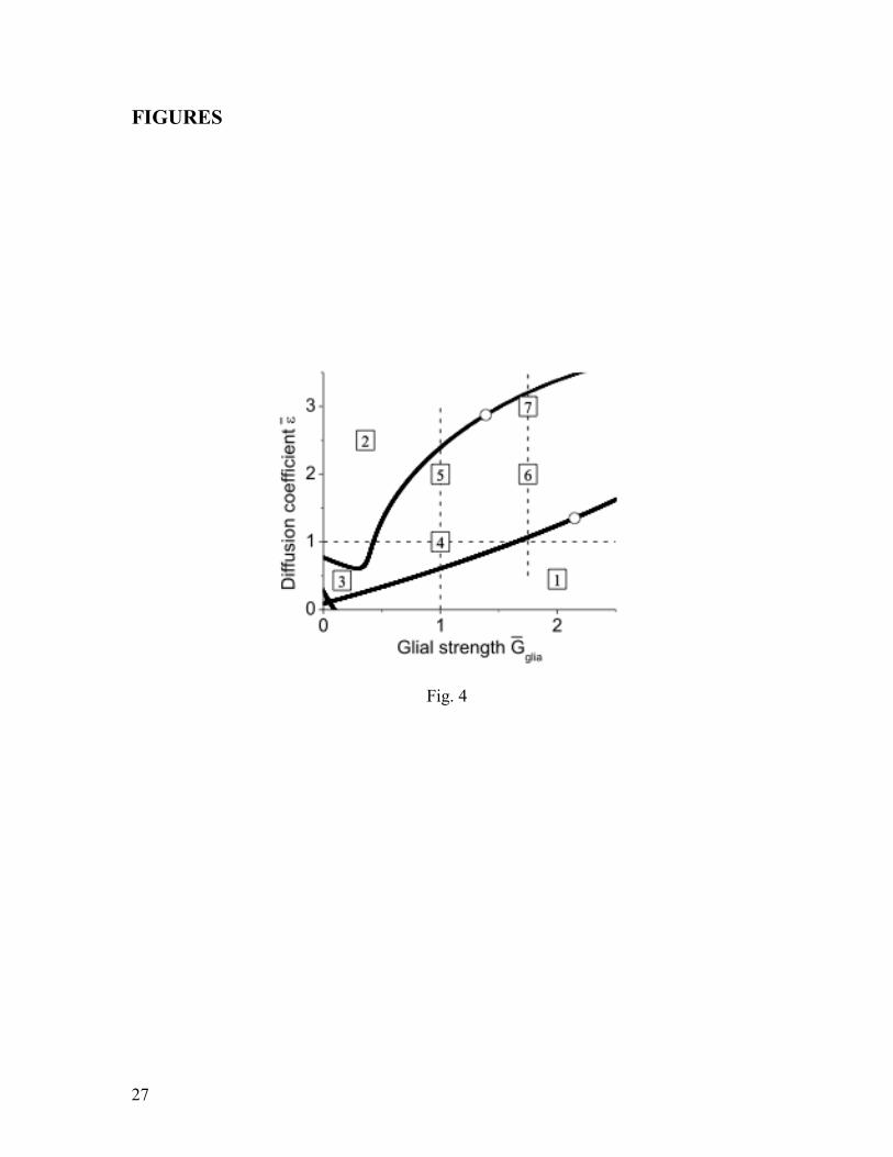
Fig. 2: The bifurcation diagram for [ ]oK as a function of the bath potassium

concentration ,ok

, revealing a region of oscillatory behavior. All other parameters were

set equal to their normal values. Triangles represent equilibria (i.e., steady states), and

circles represent periodic orbits (i.e., oscillatory behavior); stability is denoted by solid

(stable) and open (unstable) symbols.

Fig. 3: Bifurcation diagrams for [ ]oK as a function of (a) the normalized pump strength,

(b) the diffusion coefficient, and (c) the glial strength. All plots were produced with an

elevated bath potassium concentration at k

o, 2.0 .

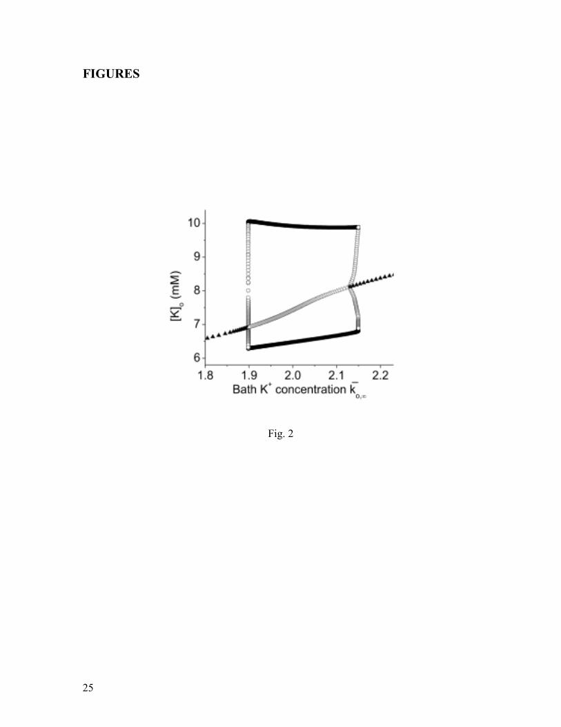
Fig. 4: A two-dimensional bifurcation diagram showing the boundaries of the region of

oscillation (RO) as a function of the diffusion coefficient and the glial strength. The black

curves denote Hopf bifurcations; within this region, the ion concentrations exhibit

oscillatory behavior. The dashed lines correspond to the one-dimensional bifurcation

diagrams in Figures 3b, 3c and 5 (see text). Examples of the dynamics of the full model,

obtained at parameter values corresponding to the numbered points, are shown in Figure

6.

Fig. 5: The one-dimensional bifurcation diagram for [ ]oK as a function of the normalized

diffusion coefficient for k

o, 2.0and

gliaG = 1.75.

20

Fig. 6: Examples of the dynamics of the full model, obtained at parameter values

corresponding to the numbered points in Figure 4. The top trace shows the membrane

voltage and the lower traces show [K]o (solid trace) and [Na]i (dashed trace) on the same

time scale.

Fig. 7: The effect of changing the bath concentration on the location of the region of

oscillation (RO) is illustrated for 1 and various values of the bath potassium

concentration ,ok

. The square represents normal values of the diffusion and glial

strength. In (a), the RO is seen to appear and move to the right as the bath potassium

concentration is increased from k

o, 1.77 (grey curve) to

k

o,1.9 (black curve),

where it intersects the square (compare the left bifurcation in Figure 2). In (b), the normal

square lies within the RO for k

o, 2.0 . In (c),

k

o, 2.1, the RO has moved further to

the right, and the square is close to the left boundary.

Fig. 8: Other bursting patterns. Traces similar to those in Figure 6 obtained with the full

model for (a) k

o, 6.0 ,

gliaG = 0.1, and = 0.4 ; and (b) same, but with k

o, reduced

slightly. The quiescent states in (a) correspond to depolarization block; see text for

further description.

21

Table 1: Model variables and parameters.

Variable Units Description

V

INa

IK

IL

m(V)

h

n

(V)

(V)

[Ca]i

VNa

VK

[Na]o

[Na]i

[K]o

[K]i

Ipump

Idiff

Iglia

mV

A/cm2

A/cm2

A/cm2

mM

mV

mV

mM

mM

mM

mM

mM/sec

mM/sec

mM/sec

Membrane potential

Sodium current

Potassium current

Leak current

Activating sodium gate

Inactivating sodium gate

Activating potassium gate

Forward rate constant for transition between

open and close state of a gate

Backward rate constant for transition between

open and close state of a gate

Intracellular calcium concentration

Reversal potential of persistent sodium

current

Reversal potential of potassium current

Extracellular sodium concentration

Intracellular sodium concentration

Extracellular potassium concentration

Intracellular potassium concentration

Pump current

Potassium diffusion to the nearby reservoir

Glial uptake

Parameter Value Description

C

gNa

gK

gAHP

gKL

gNaL

gClL

VCl

gCa

VCa

Gglia

ko,

[Cl]i

[Cl]o

1F/cm2

100mS/m2

40mS/m2

0.01mS/m2

0.05mS/m2

0.0175mS/m2

0.05mS/m2

3sec-1

-81.93mV

0.1mS/m2

120mV

7.0

1.25mM/sec

66mM/sec

1.2sec-1

4.0mM

6.0mM

130.0mM

Membrane capacitance

Conductance of persistent sodium current

Conductance of potassium current

Conductance of afterhyperpolarization current

Conductance of potassium leak current

Conductance of sodium leak current

Conductance of chloride leak current

Time constant of gating variables

Reversal potential of chloride current

Calcium conductance

Reversal potential of calcium

Ratio of intracellular to extracellular volume

of the cell

Pump strength

Strength of glial uptake

Diffusion constant

Steady state extracellular concentration

Intracellular chloride concentration

Extracellular chloride concentration

22

APPENDIX A

Current to concentration conversion:

In order to derive the ion concentration dynamics, we begin with the assumption

that the ratio of the intracellular volume to the extracellular volume is = 7.0 (Somjen,

2004). This corresponds to a cell with intracellular and extracellular space of 87.5% and

12.5% of the total volume respectively. For the currents across the membrane,

conservation of ions requires

c

iVol

i c

oVol

o,

where c and Vol represent ion concentration and volume respectively, indicates change,

and the subscripts i, o correspond to the intra- and extracellular volumes. The above

equation leads to

ci c

o

Volo

Voli

co

.

Let I be the current density in units of A/cm2 from the Hodgkin-Huxley model.

Then, the total current itotal

IAentering the intracellular volume produces a flow of

charge equal to Q i

totalt in a time t , where A is membrane area. The number of ions

entering the volume in this time is therefore N i

totalt / q where q is 1.6x10

-19 coul.

The change in concentration c

i N / N

AVol

i depends on the volume of the region to

which the ions flow, where Avogadro’s number NA converts the concentration to molars.

The rate of change of concentration, or concentration current dc

i/ dt i

c,i, is related to

the ratio of the surface area of the cell to the volume of the cell as follows

ic,ic

i

t

N

tVoliN

A

itotal

qVoliN

A

IA

qVoliN

A

I

.

For a sphere of radius 7m, = 21mcoul/M.cm2. An increase in cell volume

would result in a smaller time constant and therefore slower dynamics.

For the outward current the external ion concentration is therefore given as

, , 0.33c o c i

Ii i I

23

Equations for reduced model:

The reduced model uses empirical fits of the average membrane currents of the Hodgkin-

Huxley model neuron, as described in the main text. The fits are given below.

I

K

K(g

1g

2g

3 g

lK)

I

Na

Na(g

1g

2g

3 g

lNa)

K

o/ i [K]

o/ [K]

i

Na

i/o [Na]

i/ [Na]

o

g

1 420.0(1-A

1(1-B

1exp(-

1Na

i/o))1/3)

g

2 exp(

2(1.0-

2K

o/i)/(1.0+exp(-

2Na

i/o)))

g

3 (1/(1+exp(

3(1.0+

3Na

i/o-

3K

o/i)))5)

g

4 (1/(1+exp(

4(1.0+

4Na

i/o-

4K

o/i)))5)

g

lK=A

lKexp(-

lKK

o/i)

g

lNa=A

lNa

where

K 1.0,

Na 1.0, A

1 .75, B

1 .93,

1 2.6,

2 7.41,

2 2.0,

2 2.6,

3=35.7,

3 1.94,

3=24.3,

4=.88,

4 1.48,

4=24.6,A

lNa 1.5,A

lK 2.6,

lK=32.5

24

FIGURES

Fig. 1

25

FIGURES

Fig. 2

26

FIGURES

Fig. 3

27

FIGURES

Fig. 4

28

FIGURES

Fig. 5

29

FIGURES

Fig. 6

30

FIGURES

Fig. 7

31

FIGURES

Fig. 8