The Influence of Market Wages and Parental History …ftp.iza.org/dp1771.pdf · The Influence of...

IZA DP No. 1771

The Influence of Market Wages and ParentalHistory on Child Labour and Schooling in Egypt

Jackline Wahba

DI

SC

US

SI

ON

PA

PE

R S

ER

IE

S

Forschungsinstitutzur Zukunft der ArbeitInstitute for the Studyof Labor

September 2005

The Influence of Market Wages and Parental History on Child Labour

and Schooling in Egypt

Jackline Wahba University of Southampton

and IZA Bonn

Discussion Paper No. 1771 September 2005

IZA

P.O. Box 7240 53072 Bonn

Germany

Phone: +49-228-3894-0 Fax: +49-228-3894-180

Email: [email protected]

Any opinions expressed here are those of the author(s) and not those of the institute. Research disseminated by IZA may include views on policy, but the institute itself takes no institutional policy positions. The Institute for the Study of Labor (IZA) in Bonn is a local and virtual international research center and a place of communication between science, politics and business. IZA is an independent nonprofit company supported by Deutsche Post World Net. The center is associated with the University of Bonn and offers a stimulating research environment through its research networks, research support, and visitors and doctoral programs. IZA engages in (i) original and internationally competitive research in all fields of labor economics, (ii) development of policy concepts, and (iii) dissemination of research results and concepts to the interested public. IZA Discussion Papers often represent preliminary work and are circulated to encourage discussion. Citation of such a paper should account for its provisional character. A revised version may be available directly from the author.

mailto:[email protected]

IZA Discussion Paper No. 1771 September 2005

ABSTRACT

The Influence of Market Wages and Parental History on Child Labour and Schooling in Egypt∗

This paper examines the influence of adult market wages and having parents who were child labourers on child labour, when this decision is jointly determined with child schooling, using data from Egypt. The empirical results suggest that low adult market wages are key determinants of child labour; a 10 percent increase in the illiterate male market wage decreases the probability of child labour by 22 percent for boys and 13 percent for girls. The findings also indicate the importance of social norms in the inter-generational persistence of child labour: parents who were child labourers themselves are on average 10 percent more likely to send their children to work. In addition, higher local regional income inequality increases the likelihood of child labour. JEL Classification: J13, J20, O15 Keywords: child labour, child schooling, wages Corresponding author: Jackline Wahba Economics Division University of Southampton Southampton, SO17 1BJ United Kingdom Email: [email protected]

∗ I would like to thank Sally Srinivasan and Yves Zenou for helpful comments. I am grateful to Barry McCormick for valuable comments and suggestions.

mailto:[email protected]

1. Introduction

The most recent estimates by the ILO indicate that there are about 211 million

children, less than 14 years old, working world-wide.1 Many of these children work long

hours under hazardous conditions and all receive a low wage. Despite public concern for

the prevalence of child labour, there is widespread disagreement on the desirability, and

indeed feasibility, of banning child labour. The formulation of effective policies to tackle

child labour requires the accumulation of further empirical evidence on the main causes

and consequences of child labour.

A ban on child labour may be welfare reducing for both children and parents if poverty

is the main cause of child labour. In a seminal paper, Basu and Van (1998) show that in

poor countries where market wages are low, banning child labour can worsen household

welfare. In their model, parents are assumed to be altruistic and send their children to

work only if their non-child labour income is below a tolerable level. However, empirical

studies testing this “luxury axiom” fail to consistently find a negative relationship between

household income and child labour, for example Ray (2000) and Bhalotra (2001). Unlike

previous studies, this paper is not interested in testing the luxury axiom i.e. the impact of

household income/poverty on child labour, but in providing empirical evidence on the

sensitivity of household supply of child labour to adult market wages. There are no

empirical studies which use individual level data to study the impact of adult market

wages on child labour.

The main motivation behind studying the influence of adult market wages on child

labour is its potential policy implications. For example, whether minimum wage laws can

ameliorate child labour, hinge on the sensitivity of child labour to adult market wages- see

Basu (2000). Also, targeting poor regions or deprived geographical areas, where wages are

low, may be a more practical and viable policy than targeting poor individual households

2

since it is potentially easier to get information on market wages compared to collecting

accurate data on individual households’ income and because targeting working children

might lead parents to sending their children to work in order to receive the subsidy or the

cash benefit.

This paper aims to provide empirical evidence on the influence of adult market wages

on the household decision to supply child labour while controlling for household specific

characteristics. This is implemented by using a national individual level data-set and by

exploiting the spatial variation in market adult and child wages in order to identify the

wage elasticity of household child labour supply by a representative household. Hence the

paper will address the following two questions. Are households more likely to send their

children to work if they live in regions where wages are low? How sensitive is

households’ supply of child labour to market adult wages? In addition, the paper

contributes to the child labour literature by exploring two issues that have had received

very little attention: the influence of having parents who were child labourers themselves

on the inter-generational persistence of child labour, and the impact of local regional

income inequality.

One of the disconcerting aspects of child labour is that it is often performed at the

expense of education. However, Ravallion and Wodon (2000) question the view that child

labour comes largely at the expense of schooling.2 Schooling and employment for children

are not mutually exclusive. Many children have to work in order to go to school;

otherwise they could not afford to go to school.3 This combination of school attendance

and work is facilitated by the provision of shift schools in many developing countries.4

Given the close relationship between the schooling and work choices, this study explores

the variables of interest in a model that jointly determines child labour and child

schooling, and tests for the interdependence of these two decisions.

3

This paper examines the case of Egypt using a nationally representative data set,

covering 10,000 households and more than 10,000 children. Egypt is well-suited for our

analysis because work and school combination among Egyptian working children is

common practice - more than half of the working children combine working and

schooling. In addition, Egypt is not an outlier or an extreme case of child labour. The ILO

estimates in 1995 show that the economic activity rates in Egypt, among 10 to 14 years

old was around 11.2 % - which is higher than the regional average for Latin America

(9.8%), but less than that for Africa (26.2%) and Asia (12.8%)- though there is a wide

variation in the participation rates of 10-14 years old children within the same region.

The plan of the paper is as follows. Section 2 reviews the literature on child labour.

Section 3 describes the characteristics of child labour in Egypt. Section 4 presents the

econometric model used. The main determinants of child labour and school participation

are reported in Section 5. The main findings and policy implications are summarized in

Section 6

2. Literature Review

One recent and notable theoretical contribution to the child labour literature is Basu and

Van (1998) which is used to motivate the empirical analysis in this paper. Basu and Van

(1998) assume that parents send their children to work only if they are poverty stricken–

the luxury axiom. They take for granted parental altruism towards the child. Thus, in their

model, a household only sends children to work if the household’s income (from non-

child-labour sources) is very low because adult wages are low. In their model, children

allocate their time between work and leisure where leisure is a luxury good. In addition,

they assume that from the employers’ point of view, adults and children are substitutes-

the substitution axiom. These two assumptions imply that if any individual household

4

withdraws its children from work, the household will face acute poverty. But if all

households withdraw all children from the labour market, given they assume that adults

and children are substitutes, this will cause the demand for adults to rise and the wage rate

of adult labour to increase. But if adult wages were at this higher level to start with, then

the parents would not have sent their children out to work in the first place. They argue

that if a labour market is characterised by more than one equilibrium – one in which adult

wages are low and children work, and another where adult wages are high and children do

not work- banning child labour is a benign policy. But, in very poor countries, where there

is only one labour market equilibrium at which adult wages are low, banning child labour

can worsen the households' welfare.

Few studies have extended Basu and Van (1998) by examining the dynamics of child

labour, for example, Basu (1999) and Emerson and Souza (2003). Those models take into

account the trade off between child labour and schooling. Thus, they assume that child

labour is undertaken at the expense of human capital formation and would lead to child

labour trap: if children work, they will not go to school and will have low human capital.

As adults, they will also need to send their children to work thereby perpetuating child

labour in the future.

Other studies have emphasised the role played by credit market imperfection. For

example, Baland and Robinson (1999) show how inefficient child labour could arise

despite parental altruism when capital markets are imperfect. Ranjan (1999) also shows

that the non-existence of market for loans against the future earnings of children gives rise

to inefficient child labour because child labour acts as a consumption smoothing device

for poor households in the absence of credit markets.

A few empirical studies have attempted to test Basu and Van’s (1998) luxury axiom in

which they assume that households only send their children to work if they are poverty

5

stricken. Nevertheless, those studies do not consistently find a negative relationship

between household income and child labour. For example, Ray (2000a) finds mixed

evidence; a positive significant relationship between household poverty and child labour

in the case of Pakistan, but not in the case of Peru. Nielsen (1998) finds that in the case of

Zambia, poverty and low income have very small effects on the probability of child

labour, and concludes that poverty is not the main cause of child labour in Zambia.

Canagarajah and Coulombe (1997) also find that household welfare has a weak effect on

the probability of child labour in Ghana. Bhalotra and Heady (2003) find a negative

income effect for boys in Pakistan, but they find no evidence that the work of girls in

Pakistan, or the work of boys and girls in Ghana, is sensitive to household income. Most

of these studies treat household income as exogenous- except for Bhalotra and Heady

(2003) and Bhalotra (2001).5 However, parents' income is most likely to be endogenous-

since whether children work, or not, is likely to influence parents’ reservation wages and

the labour market participation of the parents. Another potential problem with using

household income is that it might not always reflect household welfare in developing

countries, in particular in those societies where subsistence agriculture is common and

households consume what they produce.

Unlike previous studies, this paper is not concerned with testing the luxury axiom,

but in providing empirical evidence on the sensitivity of household supply of child labour

to adult market wages. The main focus in this paper is on market wages as opposed to

household wages or income. As discussed above, Basu and Van (1998) stress the role of

adult market wage; they assume that households send children to work only if the adult

market wage is very low and as the wage rise they withdraw their children from the labour

force. Thus, the elasticity of child labour supply to market adult wages is important in

particular for policy formulation. Hence, understanding if households are more likely to

6

send their children to work if they live in regions where wages are low would help in

devising effective policies to deal with child labour. There are no empirical studies using

individual level data that examine the impact of adult market wages on child labour.

Although Ray (2000b) investigates the impact of wages on the responsiveness of hours of

child labour, he uses the maximum wage attracted by the female, male and child workers

in the household and not market wages.

Earlier studies using aggregate data -Rosenzweig and Evenson (1977), Rosenzweig

(1981), Levy (1985), and Skoufias (1994) - focus on the trade-off between the number and

the quality of children in rural areas.6 The resulting evidence on the impact of adult market

wages is inconclusive. Rosenzweig and Evenson (1977) using aggregate district level data

from rural India in the 1960s, find that both adult male and female wages have negative

significant impact on boys and girls working. On the other, Skoufias (1994) using

aggregate data from six villages in India but for the 1970s, find that adult wages do not

have a significant influence on the probability of child participation in either the labour

market or schooling. Levy (1985) using aggregate provincial level data from rural Egypt,

though not distinguishing between boys and girls, shows that higher adult male wages

have positive significant effect on child labour, while adult female wages have negative

one,7 but his focus is on the impact of cropping pattern and mechanisation on child labour

and fertility in rural Egypt.

The second focus of this paper is on the inter-generational persistence of child

labour and the influence of parents who worked as child labourers. The literature on the

"underclass" has emphasized the extent to which poverty is passed from one generation to

another in the United States. The large impact of family background on income status has

been stressed by several studies, for example, Corcoran et al. (1990). Solon (1999) points

out that it is conjectured that intergenerational transmission of economic status is

7

particularly strong, and mobility is lower, in LDCs. However, there is little empirical

evidence on the intergenerational transmission of economic status, income or poverty in

developing countries, in particular, on how child labour perpetuates poverty from one

generation to another, or on how parents who were child labourers are more likely to have

their children work as well. There are two recent exceptions. First, Ilahi, Orazem and

Sedlacek (2000) examine the effect of child labour on lifetime earnings and poverty status

using retrospective data on adult earnings and information on whether adults worked as

children in Brazil. They find that entry in the workforce before age 13 results in a

reduction in adult wages of 13-17 percent and an increase in the probability of being in the

lowest two income quintiles of 7-8 percent. They estimate the effect of child labour both

independent of its effect on education and through its effects on education. They find both

effects to be significant. They argue that early entry in the labour force reduces years of

education and lowers the returns per year of schooling. Their focus is on the implications

of child labour on wages, income and poverty. They do not study the intergenerational

persistence of child labour; i.e. whether those who worked as children also had parents

who worked as children. Secondly, a recent paper by Emerson and Souza (2003) explore

the evidence of intergenerational persistence of child labour. They build an overlapping

generation model of the household child labour decision to capture a child labour-trap

story and then examine the empirical evidence using household survey data from Brazil.

They find that adults who worked as children have lower earnings even when controlling

for their educational levels and that the likelihood of being child labourer increases the

younger the parents entered the labour market. Although they control for parental

education and household income- which is endogenous-, the intergenerational persistence

of child labour remains. They explain the persistence of child labour above that of parental

education and household income, given their theoretical model, to be the result of some

8

unobservable human capital characteristic i.e. human capital accumulation is not

determined only by the amount of education but also by maybe the quality of education,

the level of education of siblings or the household environment. In other words, they

focus on the child labour-poverty trap explanation. However, this paper suggests a

different explanation for the intergenerational persistence of child labour, namely social

norms, as discussed below.8

The relationship between family background, such as race, ethnic origin, religion

and in particular education, and child labour is fairly established in the empirical

literature- see Grootaert and Kanbur (1995). Studies show that a low level of parents’

educational attainment is an important factor in increasing the likelihood of children

working. One might argue that parents who worked as children are more likely to have

under-invested in schooling and become poverty trapped and hence would expect their

children to work as well i.e. the child labour-poverty trap explanation. Yet, what is

interesting to explore is whether the effect of having parents who were child labourers will

exist even after controlling for parents’ education. If there is still evidence of inter-

generational persistence of child labour then, it has to be for reasons beyond those which

affect human capital and income, such as those caused by social norms.

Social norms refer to social influence that affects individual’s preferences and

therefore utility- see Basu (1999). As first argued by Lindbeck (1997) social norms

interact with economic incentives and affect rational behaviour of individuals and

households. Lindbeck (1997) shows that work norms are affected by social norms, for

example, parents may encourage good working habits in the younger generation to prevent

free-riding on the altruism of others in the future. Thus, if parents worked themselves as

children they may encourage their own offspring to work at an early age. Parents may

want their children to follow in their own footsteps and learn the parents’ craft or they

9

may attribute a positive value to contribution to family work. For example, help on the

family farm may be seen as an important value parents would like to teach their offspring.

On the other hand as argued by Lopez-Calva (1999) in some societies child labour may be

associated with a social stigma or social cost, for example shame, embarrassment or

frowning upon from others. This would be reflected in lower utility for the parents and

lower probability of household sending children to work. However, if parents worked

themselves when they were children, they may consider child labour to be the social norm,

and would associate lower social stigma with sending their children to work. The paper

explores the impact of social norms on the probability of child labour by testing whether

parents who themselves worked as child labourers are more likely to send their children to

work or not.

The third focus of this paper is the influence of unequal regional income

distribution on child labor. In Basu and Van (1998) wages are the only source of adult

income; i.e. employment is the only source of income for adults. However, in an extension

of this model, Swinnerton and Rogers (1999) allow adults in at least some households to

receive income from both wages and profits; i.e. allow some households to be

shareholders in firms. They show that child labor would also exist if non-labor income

(dividends/profits) were not equally distributed among households. They find that in

precisely circumstances where, according to Basu and Van, a ban on child labor would be

effective, child labor would exist because income is distributed unequally enough that

families still must send their children to work in order to sustain themselves.9 Ranjan

(2001) explores in a theoretical framework the relationship between inequality and child

labor, but when credit constraints exist. He shows that since borrowing against the future

earnings of children is not possible, when individuals have different abilities, unskilled

workers would send their children to work, while skilled parents would send their children

10

to school. He also shows that greater inequality is associated with greater incidence of

child labor.

However, the empirical impact of regional income inequality has not been widely

studied- as noted by Basu (1999). This paper examines the impact of income inequality,

controlling for market wages, on the probability of households supplying child labor. The

intuition here is that holding constant market wages, high income inequality driven by

unequal distribution in land ownership, assets, or other sources of non-labor income would

lead some households, to be more likely to supply child labor to compensate for their lack

of non-labor income.

3. The Data

This study uses individual level data from the 1988 Labour Force Sample Survey, a

nationally representative sample of 10,000 households, which was carried out by the

Central Agency for Public Mobilisation and Statistics (CAPMAS) in Egypt.10 The survey

provides detailed information on the employment and socio-economic characteristics of

individuals 6 years of age or more.11 The analysis is based on 10742 children aged

between 6-14 years old for whom full information on schooling, labour participation and

parents’ characteristics are available.

A child is classified as economically active, by the International Labour

Organization (ILO), if the child is remunerated for that work, or if the output of this work

is destined for the market. This definition is also adopted here.12 Hence a child is

considered to be working whether he/she is being paid for work, or is working for his/her

family and is unpaid for work destined for the market. There are no data on household

chores activities carried out by those children. This is a limitation of the data set used, and

11

therefore of the paper, since children tend to help with child care and household chores

and may spend a considerable amount of time undertaking those activities.

***** Insert Table 1*****

Table 1 presents the descriptive statistics of the sample of children between 6-14

years old by gender. The first column provides the characteristics of all children in the

sample. Columns 2 and 3 show the characteristics of school and non-school participants.

Although school non-participation rate is 9% among boys, it is almost 24% among girls.

Almost 87% of girls who do not go to school live in rural areas. In addition, the majority

of school non-goers tend to come from families where the parents have no, or very little,

education.

Columns 4 – 7, in Table 1, display the characteristics of working and non-working

children where the reference period used was the previous year. Boys have higher labour

market participation rates than girls (22% compared to 15%). However, boys seem to have

equal participation rates in paid and unpaid work, while the proportion of girls who

participates in unpaid work (12%) is almost four times that those who are engaged in paid

work (3%). Since Egyptian labour law stipulates a minimum age for employment of 12,

two age groups are distinguished: 6-11 and 12-14 years old.13 Indeed, over 40 % of

working children are less than 12 years old. Around three-quarters of working children are

engaged in agriculture. This is consistent with evidence from other developing countries

where the majority of working children tend to work in agriculture and in non-paid work.

Among working boys who do not go to school (column 3), 53% are engaged in agriculture

and the rest in manufacturing and services, suggesting that non-school participation is

correlated with working in non-agriculture activities. Also, half of the paid working boys

12

are engaged in production (column 5). Parents of non-working children are on average

more educated than those of working children. Seventeen percent of children in female-

headed households are working for wage, while only 11% are unpaid workers. More than

half of the working children - 57% of boys and 59% of girls- come from families where

the father was child labourer. Finally, although around 20% of mothers in the total sample

were child labourers, 39% of working boys have mothers who were child labourers.


More than half the working children (57%) are also attending school. On average,

children work 5.3 hours per day and 57% of working children reported working 7 days a

week.14 Table 2 presents the child labour and schooling participation patterns of children

by gender, rural/urban areas and age groups. First, 8% of children do not work or go to

school. This group is comprised mainly of girls (83%) who are most probably involved in

household chores. Secondly, 11% of all children in the 6-14 years old cohort combine

working and studying. Many Egyptian public schools operate up to three-shift schedules

(4 hours each) a day due to government resource constraints, which seems to

accommodate for the dual activities of children. Work and study combination is more

common among boys, among 12-14 years old, and in rural areas. In fact, more boys tend

to combine working and studying (16%) compared to only working (7%). The majority of

children in urban areas are enrolled in schooling and only 3% work and do not go to

school.

4. The Econometric Model

13

To study how variations in market adult wages across provinces and having parents who

were child labourers affect the decisions of a representative household to supply child

labour and demand child schooling, a reduced form model is used. The estimation method

used here reflects the decision making process. Schooling and work are not treated as two

independent decisions nor as a sequential process.15 First, using a sequential choice model

would involve a number of strong assumptions concerning the hierarchy of the decision

making. The four choices of interest here are: work only, schooling only, work and

schooling, and no work & no schooling. However, there is no clear ordering of those

options. If the child's welfare is the main concern then schooling only is the first choice-

see Grootaert (1998), but if the household is poor and rely on the child for survival, then

schooling and work may become the first option. However, if the household's welfare,

rather than the child 's, is the main concern, then the ranking of the choices becomes

unclear.

Second, using a multinomial logit choice model assumes that all the options are

considered simultaneously and are independent- the assumption of independence of

irrelevant alternatives (IIA). In other words, using a multinomial logit model would imply

that the decision to work is independent from other options, and is not affected by whether

or not a schooling option is available.

In this paper, it is assumed that the decisions are interdependent and a bivarite probit

model is used because it allows for the existence of possible correlated disturbances

between the two decisions. Bivarite probit models also allow us to test for the existence

and significance of the interdependence of these two decisions.

Let the latent variable represent the decision of working and the decision of

schooling. The general specification of a two-equation model is

*1y *

2y

14

otherwiseyyifyxy 0,01, 1*1111

'1

*1 =>=+= εβ

otherwiseyyifyxy 0,01, 2*2222

'2

*2 =>=+= εβ

0][][ 21 == ii EE εε 1][][ 21 == ii VarVar εε

ρεε =],[ 21 iiCov

where ρ is the coefficient of correlation between the two equations. The first dependent

variable is defined 1 if the child is economically active in the labour market and 0

otherwise. The second dependent variable is defined 1 if the child participates in schooling

and 0 otherwise. xi1 and xi2 are the two sets of explanatory variables explaining the

probability of working and the probability of attending schooling respectively, namely

market wages and whether the parents were child labourers, in addition to the

characteristics of the child, parents, household, and region which are used as control

variables and are explained below.

i) Market Wages

First, to examine the impact of adult market wages on the household decision to

supply child labour, I exploit the variability in market wages across various labour market

areas in Egypt. Then, by controlling for households' characteristics which might influence

child labour supply, I can study how variations in market adult wages across provinces

affect the decisions of a representative household to supply child labour and demand child

schooling. Unfortunately, published statistical sources do not report wages at the level of

disaggregation needed here. I circumvent this problem by using the earnings module in the

1988 LFSS, which provides actual hours worked and wages for workers, to calculate

hourly market wages separately for the urban and rural areas of each province

(governorate), but I correct for clustering and heteroscedasticity as a result of using

individual level data.16

15

Since our interest here is in testing the sensitivity of household supply of child

labour to adult market wages especially at very low levels of wages, it could be argued that

wages of adults with no education are the most relevant ones. Table 1 shows that around

40 percent of adult males and 75 percent of adult females in our sample are illiterates.

Using the illiterate market wage is superior to using the average market wage for all

educational groups because the illiterate market wage is less noisy since it is not

influenced by the educated public sector wages and government employment which would

provide an inflated measure of the average market wage depending on the local size of the

public sector. Also, using the illiterate market wage is better than using the agricultural

wage which would only be of relevance to rural agricultural areas. In addition, for policy

intervention focusing on wages of those with no education is the most appropriate. Both

male and female adult wages are used to capture the different impact each may have on

child labour and schooling Thus, the log of adult market hourly wages of illiterate males

and females by rural and urban area in every province relative to the national average are

used.17

Also, the log of child market hourly wage by rural and urban area in every

province relative to the national average is included. Even when children are unpaid

family workers, high child wages would make it expensive for households to employ

children from outside the household, thus requiring their own children to work. On the

other hand, the effect of child market wage on the probability of child participating in

schooling is an indirect one because it is the opportunity cost of not working.

ii) Income Inequality

Since the concern here is with examining the impact of market wages on child

labour decision, I control for local income distribution using the Gini coefficient at the

16

governorate/province. The Gini coefficient is based on consumption expenditure, and thus

captures earnings as well as non-labour income and wealth.18 The intuition here is that

controlling for provincial income inequality driven by unequal distribution in land

ownership, assets, or other sources of non-labour income, one can better examine the

sensitivity of the supply of child labour to market wages.

iii) Parental history and Social Norms

To explore the impact of the parents being child labourers themselves on the probability of

the children working and/or going to school is studied by allowing for separate effects for

both the father and mother. The 1988 LFSS asks each individual the age at which they

first entered the labour market. A parent is considered a child labourer if he/she has started

labour market work at the age of 14 years old or before. One possible reason behind the

inter-generational persistence of child labour is the child labour-poverty trap explanation

which is discussed in Emerson and Souza (2003). A parent who has been raised in poor

family, where he/she had to work as child himself/herself which constrained him/her

ability to invest in schooling and condemned him/her to low wage or poverty as an adult,

will tend to send his/her children to work in turn. However, another potentially important

reason for the persistence of child labour is social norm. To capture the impact of social

norms in the intergenerational persistence of poverty rather than the influence of poverty

trap due to lack of human capital, I control for the education of the parents. Four

educational dummies are used for each parent: illiterate, less than primary (less than 6

years of basic education), primary, and more than primary education. In addition, to

control for the nature of the parents' employment and the impact of the father having a

stable regular job, a dummy variable indicating whether the father is employed in the

Public Sector is also included

17

iv) Child’s and Household’s Characteristics:

Separate estimates for boys and girls are reported since the determinants of child

labour and schooling may be gender specific. I control for the child's age, but also estimate

the model separately for 6-11 and 12-14 years old since the Egyptian labour law stipulates

a minimum age for employment of 12.

In addition I control for other household characteristics. A dummy is used to

capture the impact of female headed household. Also to control for non-labour income, a

dummy is included for whether there are any return overseas migrants in the household,

since return migrants may be less credit constrained if they have acquired overseas

savings. Finally, the number of siblings less than six years old in the household is also

included to capture the need for child care which in many instances is done by older

sisters and would affect girls’ participation in the labour force and in schooling.

v) Regional Characteristics:

Another important factor, which affects the supply of child labour, is the availability of

children's jobs. For example, child labour is higher in rural areas where children tend to

work for their families. Children are not as mobile as adults and would tend to work near

where they live. Thus, accessibility of jobs seems to be an important factor that would

affect the supply of child labour. If children are located in a province where there is no

access to jobs, one would expect that the willingness of the households to supply child

labour would be lower since the alternative would be incurring higher cost (transportation,

effort and time). To control for the accessibility of jobs in a province, three variables are

used. First, to capture the degree of informality in the local labour market the percent of

adults in non-regular – casual and seasonal - employment in the rural/urban area of the

province is used. Secondly, the share of adult workers employed in Public Sector in the

18

rural/urban area in the province is included. Finally, the percentage of adult workers

engaged in manufacturing, in the rural or urban area, in the province is used to control for

the industrial composition of the local labour market. However, the model was also

estimated without these three labour market variables, and the results were unchanged.

One of the limitations of the data set used in this paper is the lack of information

on variables that may affect the demand for schooling, for example, school availability,

accessibility (distance to school), quality of schooling, and cost of schooling. Previous

studies - for example, Bonnet (1993) and Hanushek and Levy (1993) - point to the

importance of school accessibility and school quality in determining the schooling

participation decision. So, six regional dummies capturing the household’s region of

residence are used to control for school availability and quality in the school participation

equation: Greater Cairo, Alexandria and Canal Cities, Lower Urban, Upper Urban, Lower

Rural and Upper Rural. One would expect that in rural areas because of poor schooling

facilities, children would be less likely to attend school compared to in urban areas. In

addition, children in the poorer rural areas - the south (Upper Rural Egypt) - are expected

to have lower probability of going to school compared to children in other rural areas - in

the north (Lower Rural Egypt).

5. Empirical Findings

Before discussing the empirical findings, it is important to examine whether the estimation

technique adopted here is the best one to model the two decisions under study. A

multinomial model was estimated and Hausman's test was carried out to test for the

independence of irrelevant alternatives assumption (IIA). The results of the Hausman’s

test rejected that assumption indicating that a multinomial model would not have been

appropriate. Using bivarite probit estimation, the correlation coefficient ρ is found to be

19

significant in all the models implying that working and schooling are not independent and

thus the choice of this estimation technique is appropriate. In addition, the correlation

coefficient ρ is negative and significant indicating that there is a trade-off between child

labour and child schooling choices, which is bigger in urban areas, and for males.


First, the impact of market wages is examined. The findings in Table 3 show a

strong negative relationship between illiterate adult male and female market wages and

child participation in the labour market: the higher the adult male and female provincial

wages relative to the national average, the lower is the probability of child labour. It is

interesting to note that this negative relationship exists for both boys and girls for both

paid and unpaid work (Table 3), in rural and urban areas (Tables 3 & 4), and for both age

groups: 6-11 and 12-14 years old (Table 5). In addition, the findings also indicate that the

higher is the child market wage, the more likely a child will work.

***** Insert Tables 4 and 5 *****

To check the robustness of these results, two tests are undertaken. First, I examine

the responsiveness of households’ child labour supply to market wages for those

households who are potentially close to the threshold of a subsistence level and restrict the

sample to those households where both parents are illiterates. The effect of illiterate adult

market wages on the labour market participation of children of illiterate parents are shown

in Table 6. The results support the previous findings and also indicate that the

20

responsiveness of child labour participation to adult market wages is stronger for those

children who come from households where both parents are illiterate.


Secondly, a tobit model is used to estimate the determinants of the number of

weekly hours of child labour. The same set of explanatory variables are included. The

uncensored sample is limited to only 1154 child workers (out of 1988) for whom the

number of weekly hours worked are available. Table 7 shows that there is a negative

relationship between male and female illiterate adult wages and weekly hours of child

work and provide further evidence in support of the previous findings.


The influence of illiterate adult male market wage on the probability of schooling

is not only positive and significant, but also has bigger impact than the adult female

illiterate market wage. The higher the provincial male market wage, relative to the

national average, the more are the odds of child attending schooling. Adult female market

wages have positive, but smaller impact on the likelihood of school participation of boys

compared to adult male market wage. However, adult female market wage has negative

impact on the schooling decision of girls. The higher the adult female wage, the lower is

the probability of female school participation. One explanation is that higher female adult

wages increase female labour market participation outside the household, which in turn

may mean that daughters are needed at home to do household chores instead of the

mother. The child market wage does not seem to have significant effect on the child

schooling decision, though it has the expected negative impact suggesting that the higher

21

the child market wage, the greater is the opportunity cost of attending schooling.19 In the

case of girls, though, it appears that the opportunity cost of their schooling is not their

own forgone wages, but those of their mothers (adult females).

***** Insert Tables 8 and 9*****

Table 9 summarises the influence of illiterate adult market wages on the

probability of child participation in the labour force by gender and region. It displays the

changes in the predicted probability of child labour - given in Table 8 Column 2- as a

result of a 1 percent change in the provincial adult market wage relative to the national

average. A 10 percent increase in the male illiterate market wage decreases the

probability of child labour by 21.5 percent for boys and 13.1 percent for girls, while, a

similar rise in female illiterate wage rate, lowers the probability of child participation in

the labour market by 18.5 percent for boys and 4.3 percent for girls. In rural areas, a 10

percent increase in female illiterate wage, decreases the likelihood of child labour by 19.0

percent for boys and 7.2 percent for girls. Also, another important finding is that the

impact of adult market wages is bigger for the 12-14 years old than for the 6-11 group. In

other words, lower adult wages increase the probability of child labour among the 12-14

years old by more than it does for the younger children.

It is interesting to compare these results to previous findings, though caution is

required since those studies are all based on aggregate level data, and they estimate

simultaneously fertility and child work. Levy (1985) finds that a 10 percent increase in

female market wage rates reduces employment of children by 27 percent for 6-11 years

old and by 15 percent for 12-14 years old, in rural Egypt. However, he finds that an

increase in male wage rates increases employment of children. 20 Rosenzweig (1981) finds

that in rural India, a 10 percent increase in adult male wages reduces boys' labour supply

22

by 10 percent, but have no effect on girls, while a 10 percent increase in adult female

wages decreases girls' participation in the labour market by 9-10 percent, but have no

effect on boys' employment. Thus, using individual level data provide a clearer and more

robust picture, than those provided by aggregate (village or district) level data, of the

influence of market wages on child labour.

To sum up, illiterate adult market wages seem to (i) have strong negative influence

on the probability of paid and unpaid child work, (ii) have greater impact in rural areas

than in urban areas, (iii) have smaller absolute effect on the probability of school

participation compared to on child labour. Low market wages seem to be one of the key

determinants of child labour.

The second main finding of the paper is that having a parent who was child

labourer increases the probability of the child working. This effect exits even though we

are controlling for parents’ education. Thus, this suggests that the inter-generational

persistence of child labour has to be for reasons beyond those of human capital and its

implications on income. Hence, the findings indicate that social norms may be responsible

for the persistence of child labour. The effect of having a mother who was child labourer

is twice as much as that of having a father who was child labourer for both boys and girls.

Having a mother who was child labourer increases the likelihood of child labour by 10

percent for boys, while having a father who was child labourer increases the probability of

child work by 5 percent. It is also interesting to note that the impact of parents being child

labourers is bigger on the 12-14 years old than on the younger group. However, having a

parent who worked as a child labourer does not significantly affect the likelihood of child

schooling.

Turning now to the effect of income inequality, the results indicate that living in a

province where there is greater local income inequality raises the probability of child

23

labour. This finding is robust in both urban and rural areas, and for both genders. Thus, the

evidence supports the existence of a positive relationship between income inequality and

child labour.

Parents’ characteristics play an important role in influencing the working and

schooling decisions of children. Having a father who is employed in the Public sector

increases the probability of the child attending school and decreases that of working.

Moreover, having less educated parents increase the likelihood of child labour and

decreases that of investing in schooling. As found in earlier studies, father's education

affects boys more than mother’s education, while the opposite is true for girls. The

empirical findings also suggest that household characteristics influence child labour and

schooling. Living in a household where the head is female, does not affect the probability

of participating in the labour market, but it increases the likelihood of investing in

schooling. Having younger siblings at the household increases the odds of child labour

and decreases that of schooling. The presence of return overseas migrants at the household

has negative (though not always significant) effect on the likelihood of child work. This

variable is capturing the effect of non-labour income, namely, overseas savings and

remittances. However, having a return overseas migrant has positive impact on the

schooling decision. This suggests that return migrants tend to invest in education.

The characteristics of the local labour market seem to have bigger impact on the

probability of child labour in rural areas than in urban ones. The findings indicate that

local labour market characteristics affect the probability of paid child labour in both urban

and rural areas. The higher the share of adults engaged in manufacturing, the lower is the

probability of child participation in the labour market, though it is more significant for

girls than boys. In other words, the share of adults engaged in manufacturing has negative,

though insignificant, impact on boys' work. Also, the share of adults employed in the

24

public sector in the local labour market has strong negative impact on child labour for both

genders. The percentage of adults engaged in non-regular employment has a positive

significant influence on the likelihood of paid child labour. Those two variables capture

the degree of informality in the local labour market and suggest that the higher the

informality in the labour market, the more likely children would work. However, the

models were also estimated without these labour market variables and the results were

unchanged.

6. Conclusion

Understanding the main determinants of child labour is essential for formulating

effective policies in tackling child labour. This paper provides empirical evidence on the

influence of market wages and having parents who were child labourers on the decision to

supply child labour. The estimates are drawn from a model in which child labour is

allowed to be jointly determined with child schooling.

The main findings of the paper are the following. Market adult wages have a

strong negative influence on the probability of child working. In addition, parents who

were child labourers themselves are on average 10 percent more likely to send their

children to work. Higher income inequality within a province/ region also increases the

likelihood of child labour. There is a trade-off between child labour and child schooling.

To sum, the empirical findings suggest that low adult market wages are key determinants

of child labour, and that social norms may be responsible for the inter-generational

persistence of child labour.

Several policy implications emerge from this paper. First, since child labour is

found to be sensitive to local market illiterate adult wages, then a viable policy would be

to target provinces or regions where illiterate adult wages are low. One policy option to

25

reduce child labour and increase child schooling would be to provide cash transfers to

children to attend school in low wage provinces. For example, Mexico introduced a

similar social program – PROGRESA- which provides cash transfers linked to children’s

enrolment and regular school attendance which has been successful in increasing school

enrolment and reducing child labour. This suggested policy has several advantages. First,

providing cash transfers to children in low wage provinces unlike, for example, increasing

minimum wages will not lead to higher adult unemployment. In addition, raising female

adult wages might lead as suggested by the empirical findings to lower probability of girls

participating in schooling since girls may be kept at home to do the household chores

instead of the mother. Furthermore, such cash transfers can be gender and age specific.

For example, the results show that work amongst children 12-14 years old is more

sensitive to the explanatory variables and household characteristics than that for younger

children, 6-11. Thus, higher cash transfers to the 12-14 years old could be used to reduce

child labour for that age group to entice them to carry on going to school. In fact, the size

of the PROGRESA benefit grant increases through grades and at the secondary level

grants are higher for females who are more likely to drop-out of school. Finally, since

policies that reduce the current child labour supply therefore also serve to reduce child

labour in future, the results suggest that returns to such policies in terms of reductions in

child work are greater than hitherto perceived.

26

7. References

Baland J-M, Robinson J (2000) Is child labour inefficient? Journal of Political Economy 108: 663-679. Basu K, Van PH (1998) The economics of child labour. The American Economic Review 88: 412- 427. Basu K (1999) Child labour: cause, consequence, and cure, with remarks on international standards. Journal of Economic Literature 37: 1083-1119. Basu K (2000) The intriguing relation between adult minimum wage and child labour. Economic Journal 110: c50-c61. Bhalotra S (2001) Is child work necessary? The World Bank Social Protection Discussion Paper No. 0121, The World Bank, Washington, D.C. Bhalotra S, Heady C (2003) Child farm labour: the wealth paradox. World Bank Economic Review, 17 (2): 197-227. Bonnet M (1993) Child labour in Africa. International Labour Review 132: 371-389. Canagarajah S, Coulombe H (1997) Child labour and schooling in Ghana. The World Bank Working Paper Series, No. 1844, The World Bank, Washington, D.C. Corcoran M, Gordon R, Laren D, Solon G (1990) Effects of family and community background on economic status, The American Economic Review, Papers and Proceedings, 80:362-366. Diamond C, Fayed T (1998) Evidence on substitutability of adult and child labour. The Journal of Development Studies 34: 62-70. Emerson PM, Souza AP (2003) Is There a Child Labour Trap? Intergenerational Persistence of Child Labour in Brazil. Economic Development and Cultural Change 51: 375-398. Egypt Human Development Report 1994. (1994) Institute of National Planning, Cairo. Fergany N (1991) Final Report. Overview and General Features of Employment in the Domestic Economy. CAPMAS, Cairo. Grootaert C (1998) Child Labour in C⊥te d’Ivoire: Incidence and determinants. The World Bank Social Development Department, The World Bank, Washington, D.C. Grootaert C, Kanbur R (1995) Child labour: an economic perspective. International Labour Review 134: 187- 580. Hanushek EA, Levy V (1993) Dropping out of school: further evidence on the role of school quality in developing countries. Rochester Centre for Economic Research Working Paper No 345, University of Rochester.

27

Ilhai N, Orazem P, Sedlacek G (2000) The Implications of Child Labour for Adult Wages, Income and Poverty: Retrospective Evidence from Brazil. The World Bank, mimeo. International Labour Organization. (2002). Every Child Counts: New Global Estimates on Child Labour, IPEC, ILO: Geneva. Jensen P, Nielsen HS (1997) Child labour or school attendance? Evidence from Zambia. Journal of Population Economics 10: 407-424. Levy V (1985) Cropping pattern, mechanization, child labour, and fertility behaviour in a farming economy: rural Egypt. Economic Development and Cultural Change 33: 777-791. Moulton BR (1990) An illustration of a pitfall in estimating the effects of aggregate variables on micro units. The Review of Economics and Statistics 72: 334-338. Nielsen HS (1998) Child labour and school attendance: two joint decisions, University of Aarhus Working Paper 98-15. Patrinos HA, Psacharopoulos G (1997) Family size, schooling and child labour in Peru, Journal of Population Economics 10: 387-405. Ranjan P (1999) An economic analysis of child labour. Economics Letters 64: 99-105. Ranjan P (2001) Credit constraints and the phenomenon of child labour. Journal of Development Economics 64: 81-102. Ravallion M, Wodon Q (2000) Does child labour displace schooling? Evidence on behavioural responses to an enrolment subsidy? The Economic Journal 110: c158-c175. Ray R (2000a). Analysis of child labour in Peru and Pakistan: a comparative study. Journal of Population Economics 13: 3-19. Ray R (2000b) Child labour, child schooling, and their interaction with adult labour: empirical evidence for Peru and Pakistan. The World Bank Economic Review 14: 347-367. Rosenzweig M, Evenson R (1977) Fertility, schooling, and the economic contribution of children in rural India: an econometric analysis. Econometrica 45: 1065-1079. Rosenzweig M (1981) Household and non-household activities of youths: issues of modelling, data and estimation strategies. In: Rodgers G, Standing G (eds) Child work, poverty and underdevelopment, ILO, Geneva 215-244. Siddiqi F, Patrinos HA (1995) Child Labour: Issues, Causes and Interventions, Human Resources Development and Operations Policy, Working Paper No. 56, The World Bank, Washington D.C. Skoufias E (1994) Market wages, family composition and on the time allocation of children in agricultural households. The Journal of Development Studies 30: 335-360.

28

Solon G (1999) Intergenerational mobility in the labour market. In Ashenfelter O, Card D (eds) Handbook of Labour Economics, Vol. 3A, Elsevier, North-Holland. Swinnerton KA, Rogers CA (1999) The economics of child labour: comment. The American Economic Review 89: 1382-1388. Swinnerton, KA, Rogers, CA (2000) Inequality, productivity, and child labour: theory and evidence. mimeo.

29

Table 1. Descriptive Statistics 1 2 3 4 5 6 7

TotalSample

School Participants

Non-School Participants

Labour Force Participants

Paid Workersb

Unpaid Workersb

Non-LF Participants

M a Fa M F M F M F M F M F M F ALL

51.2

48.8

90.6

76.5

9.4

23.5

22.2

14.5

13.9

2.7

13.8

11.8

77.8

85.5

Age (%)

6-11 66.1

66.8 68.9 71.6 41.2 52.2 41.0 44.2 28.4 47.1 48.5 43.6 73.5 70.812-14 33.9 33.2 31.1 28.4 58.8 47.8 59.0 55.8 71.6 52.9 51.5 56.4 26.5 29.2 Educational Level (%)

None 13.0 29.2 ---- ---- 77.1 89.5 27.7 58.5 38.1 59.2 20.6 58.3 5.8 21.3Read and write

57.0 46.9 66.6 66.8 13.2 7.8 40.5 26.7 30.7 30.8 47.1 25.8 65.0 52.3

Primary 30.0 23.9 33.4 33.2 9.7 2.7 31.8 14.8 31.2 10.0 32.3 15.9 29.2 26.4 Region (%) Greater Cairo 19.1 20.2 25.0 21.2 10.9 5.7 9.1 2.7 19.4 3.9 2.2 2.7 22.3 23.2Alex and Canal Cities 7.7 8.0 7.8 9.6 4.0 3.5 2.6 1.2 3.8 1.8 1.9 1.1 8.9 9.3Lower Urban 9.0 8.2 9.4 10.2 6.2 2.1 6.8 3.0 10.1 3.4 4.8 2.9 9.6 9.1Upper Urban 4.2 4.3 4.4 5.0 2.9 2.1 1.8 1.3 2.6 0.6 1.3 1.4 5.0 4.8Lower Rural 31.8 32.6 31.5 30.6 35.1 38.7 47.0 59.3 30.5 58.4 56.9 59.5 27.3 27.9Upper Rural 27.4 26.7 25.7 19.7 41.1 48.0 32.7 32.3 33.6 31.9 32.1 32.5 25.9 25.7 Industry(%)c

Agriculture --- --- 74.9 87.4 53.1 91.0 68.3 89.6 40.0 86.6 87.4 90.2 --- ---Manufacturing

--- --- 7.9 3.2 21.0 5.6 12.0 6.7 26.9 9.8 3.4 3.6 --- ---

Construction

--- --- 3.2 0.2 7.3 0.3 3.6 0.2 7.6 1.2 1.3 0 --- ---Trade --- --- 10.3 9.0 1.0 0.1 9.4 5.3 8.8 2.4 9.7 6.0 --- ---Services --- --- 3.7 0.2 12.6 0.0 6.7 0.2 15.7 0 0.1 0.1 Occupation (%)c

Sales Workers --- --- 8.7 9.5 5.0 2.9 7.7 5.4 6.7 2.4 8.2 6.1 --- ---Services Workers --- --- 2.4 0 1.6 0 2.3 0 4.0 0 1.3 0 --- ---Agricultural Workers --- --- 74.9 87.0 53.0 90.6 68.1 89.2 39.6 86.6 84.6 90.8 --- ---Production Workers --- --- 14.0 3.5 39.9 6.5 21.9 5.4 49.7 11.0 5.9 4.1 --- ---

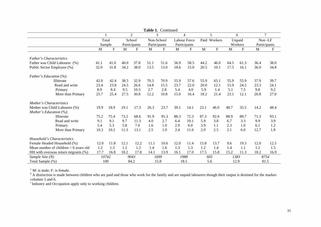
Table 1. Continued 1 2 3 4 5 6 7

TotalSample

School Participants

Non-School Participants

Labour Force Participants

Paid Workers Unpaid Workers

Non -LF Participants

M F M F M F M F M F M F M F Father’s Characteristics

Father was Child Labourer (%) 41.1 41.0 40.0 37.8

51.1 51.6 56.9 58.5 44.2 46.0 64.5 61.3 36.4 38.0Public Sector Employee (%) 32.0 31.8 34.2 38.0 13.5 13.0 18.6 15.0 20.5 10.1 17.5 16.1 36.0 34.8

Father’s Education (%):

Illiterate 42.0 42.4 38.5 32.9 70.3 70.9 55.9 57.6 55.9 65.1 55.9 55.9 37.9 39.7 Read and write 23.4 23.8 24.5 26.6 14.8 15.5 23.7 22.0 20.0 12.1 15.9 24.5 23.3 24.1 Primary 8.9 8.4 9.5 10.3 2.7 2.8 5.4 4.0 5.9 1.4 5.1 7.5 9.8 9.2 More than Primary 25.7 25.4 27.5 30.8 12.2 10.8 15.0 16.4 18.2 21.4 23.1 12.1 26.8 27.0 Mother’s Characteristics Mother was Child Labourer (%) 19.9 18.9 19.1 17.3 26.3 23.7 39.1 14.1 23.1 46.0 48.7 35.5 14.2 48.4Mother’s Education (%): Illiterate

75.2

75.4

73.2

68.6

91.9

95.3

88.3

72.3

87.3

92.6

88.9

89.7

71.3

93.1

Read and write 9.1 9.1 9.7 11.3 4.0 2.7 6.4 10.1 5.9 3.8 6.7 3.3 9.9 3.9 Primary 5.4 5.3 5.8 7.0 1.6 1.0 2.9 6.0 3.9 1.1 2.3 1.0 6.1 1.2 More than Primary 10.3 10.2 11.3 13.1 2.5 1.0 2.4 11.6 2.9 2.5 2.1 6.0 12.7 1.8 Household’s Characteristics Female Headed Household (%) 12.0 11.8 12.1 12.2 11.1 10.6 12.0 11.4 15.8 13.7 9.6 19.3 12.0 12.5Mean number of children < 6 years old 1.2 1.3 1.2 1.2 1.4 1.6 1.3 1.3 1.2 1.4 1.4 1.1 1.2 1.5 HH with overseas return migrants (%) 17.7 16.8 18.2 17.8 14.1 13.9 16.1 17.0 17.5 15.8 15.2 11.3 18.2 16.9Sample Size (N) 10742 9043 1699 1988 605 1383 8754 Total Sample (%) 100 84.2 15.8 18.5 5.6 12.9 81.5

a M: is male; F: is female. b A distinction is made between children who are paid and those who work for the family and are unpaid labourers though their output is destined for the market- columns 5 and 6. c Industry and Occupation apply only to working children.

31

Table 2. Labour Force and Schooling Participation Rate of Children 6-14 years old (%) Working and

Studying Working

Only Studying

Only Neither Total

Total Sample

10.6

7.9

73.6

7.9

100

Gender Boys 15.1 7.1 75.1 2.7 100 Girls 6.0 8.7 71.9 13.4 100 Region Urban 5.0 3.3 87.6 4.1 100 Rural 16.4 12.6 59.2 11.9 100 Age Group 6-11 years old 7.9 4.0 80.8 7.3 100 12-14 years old 15.9 15.6 59.4 9.1 100

Table 3. Determinants of Child Labour and Schooling: Rural & Urban Areas (Marginal Effects) Variable Boys Girls

Work School Paid Work

School Work School Paid Work

School

Constant -0.841

(10.03) 0.098

(12.06) -0.308 (6.80)

0.038 (12.18)

-0.317 (7.57)

0.046 (14.42)

-0.054 (4.10)

0.005 (14.41)

Market Wages Log Male wages -0.148

(3.70) 0.018 (2.35)

-0.074 (4.08)

0.009 (3.04)

-0.117 (6.34)

0.014 (4.35)

-0.018 (3.30)

0.002 (4.94)

Log Female wages -0.127 (8.17)

0.005 (1.19)

-0.036 (5.28)

0.002 (1.58)

-0.038 (4.46)

-0.004 (2.30)

-0.001 (0.52)

-0.0003 (2.32)

Log Child wages 0.070 (3.44)

-0.007 (1.52)

0.042 (3.96)

-0.003 (1.45)

0.050 (4.50)

-0.001 (0.59)

0.002 (5.96)

-0.0001 (0.56)

Local Income Inequality Income Inequality (Gini)

0.004 (3.69)

--- 0.002 (3.00)

--- 0.003 (4.72)

--- 0.001 (2.55)

---

Parents Being Child Labourers Father was Child Labourer

0.054 (5.04)

0.001 (0.28)

-0.004 (0.80)

0.0006 (0.63)

0.024 (4.25)

-0.001 (0.68)

-0.001 (0.36)

0 (0.63)

Mother was Child Labourer

0.098 (8.73)

-0.001 (0.52)

-0.004 (0.65)

-0.0001 (0.17)

0.056 (9.80)

0.001 (0.86)

0.001 (0.45)

0.0001 (0.99)

Child Characteristics Age 0.052

(25.89) -0.005 (9.94)

0.016 (18.14)

-0.002 (10.38)

0.019 (18.42)

-0.003 (14.17)

0.002 (7.20)

-0.0003 (14.22)

Father’s Characteristics Employed in Public Sector

-0.057 (4.79)

0.015 (4.57)

-0.003 (0.55)

0.006 (4.69)

-0.034 (4.90)

0.009 (6.89)

-0.003 (1.44)

0.001 (6.93)

Father's Education (ref.: illiterate) Less than Primary -0.026

(2.22) 0.021 (6.90)

-0.019 (3.47)

0.009 (7.29)

-0.013 (2.07)

0.012 (10.11)

-0.005 (2.73)

0.001 (10.20)

Primary -0.075 (3.94)

0.027 (4.91)

-0.032 (3.60)

0.011 (5.26)

---- ---- --- ----

More than Primary -0.089 (3.91)

0.040 (4.78)

-0.049 (4.70)

0.015 (4.57)

---- ---- ---- ----

Primary & more ---- ---- ---- ---- -0.073 (1.42)

0.040 (8.98)

-0.008 (2.82)

0.002 (8.78)

Mother’s Education (ref.: illiterate) Less than Primary -0.027

(1.49) 0.009 (1.77)

-0.015 (1.89)

0.003 (1.72)

-0.034 (3.23)

0.010 (4.93

-0.004 (1.48)

0.001 (4.92)

Primary or more -0.029 (1.34)

0.010 (1.45)

-0.008 (0.84)

0.004 (1.42)

-0.034 (4.37)

0.040 (5.73)

-0.010 (1.37)

0.004 (5.34)

33

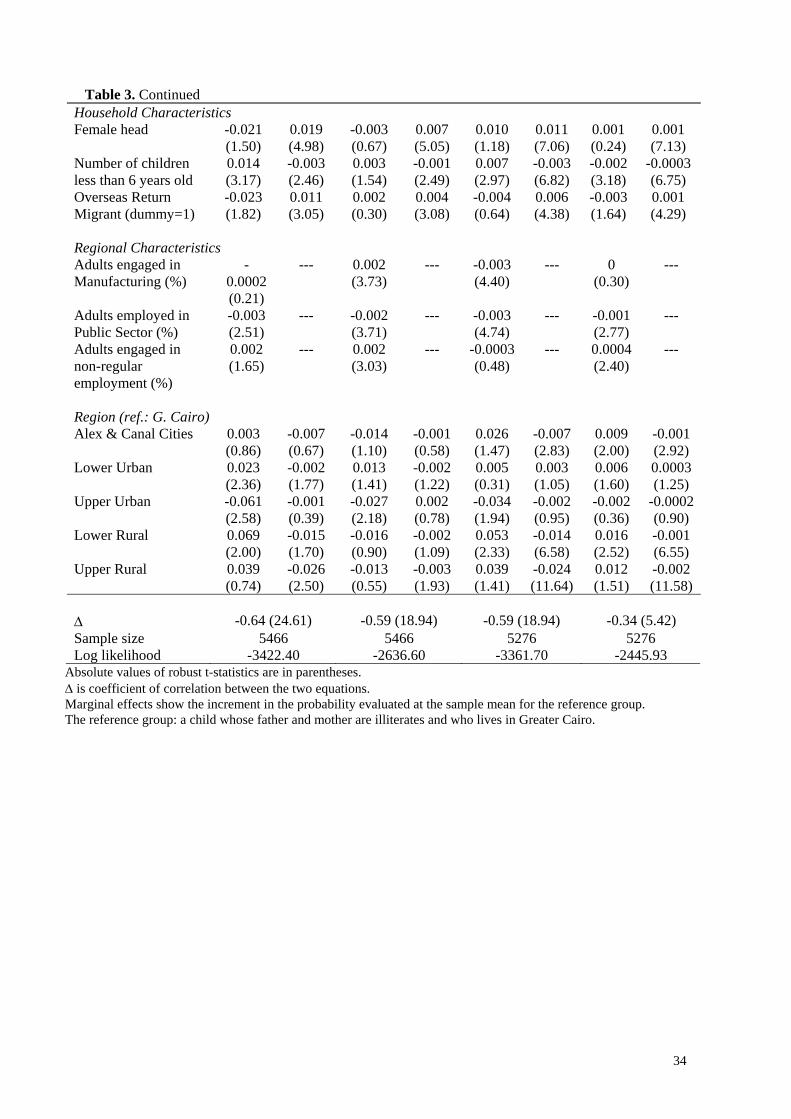
Table 3. Continued Household Characteristics Female head -0.021

(1.50) 0.019 (4.98)

-0.003 (0.67)

0.007 (5.05)

0.010 (1.18)

0.011 (7.06)

0.001 (0.24)

0.001 (7.13)

Number of children less than 6 years old

0.014 (3.17)

-0.003 (2.46)

0.003 (1.54)

-0.001 (2.49)

0.007 (2.97)

-0.003 (6.82)

-0.002 (3.18)

-0.0003 (6.75)

Overseas Return Migrant (dummy=1)

-0.023 (1.82)

0.011 (3.05)

0.002 (0.30)

0.004 (3.08)

-0.004 (0.64)

0.006 (4.38)

-0.003 (1.64)

0.001 (4.29)

Regional Characteristics Adults engaged in Manufacturing (%)

-0.0002 (0.21)

--- 0.002 (3.73)

--- -0.003 (4.40)

--- 0 (0.30)

---

Adults employed in Public Sector (%)

-0.003 (2.51)

--- -0.002 (3.71)

--- -0.003 (4.74)

--- -0.001 (2.77)

---

Adults engaged in non-regular employment (%)

0.002 (1.65)

--- 0.002 (3.03)

--- -0.0003 (0.48)

--- 0.0004 (2.40)

---

Region (ref.: G. Cairo) Alex & Canal Cities 0.003

(0.86) -0.007 (0.67)

-0.014 (1.10)

-0.001 (0.58)

0.026 (1.47)

-0.007 (2.83)

0.009 (2.00)

-0.001 (2.92)

Lower Urban 0.023 (2.36)

-0.002 (1.77)

0.013 (1.41)

-0.002 (1.22)

0.005 (0.31)

0.003 (1.05)

0.006 (1.60)

0.0003 (1.25)

Upper Urban -0.061 (2.58)

-0.001 (0.39)

-0.027 (2.18)

0.002 (0.78)

-0.034 (1.94)

-0.002 (0.95)

-0.002 (0.36)

-0.0002 (0.90)

Lower Rural 0.069 (2.00)

-0.015 (1.70)

-0.016 (0.90)

-0.002 (1.09)

0.053 (2.33)

-0.014 (6.58)

0.016 (2.52)

-0.001 (6.55)

Upper Rural 0.039 (0.74)

-0.026 (2.50)

-0.013 (0.55)

-0.003 (1.93)

0.039 (1.41)

-0.024 (11.64)

0.012 (1.51)

-0.002 (11.58)

∆

-0.64 (24.61)

-0.59 (18.94)

-0.59 (18.94)

-0.34 (5.42)

Sample size 5466 5466 5276 5276 Log likelihood -3422.40 -2636.60 -3361.70 -2445.93

Absolute values of robust t-statistics are in parentheses. ∆ is coefficient of correlation between the two equations. Marginal effects show the increment in the probability evaluated at the sample mean for the reference group. The reference group: a child whose father and mother are illiterates and who lives in Greater Cairo.

34

Table 4. Determinants of Child Labour and Schooling: Rural Areas (Marginal Effects) Variable Boys Girls

Work School Work School Constant -1.219

(11.94) 0.153 (9.49)

-0.654 (9.03)

0.147 (10.32)


(3.94) 0.040 (2.40)

-0.325 (5.82)

0.055 (4.07)


0.009 (1.56)

-0.108 (5.22)

-0.014 (2.54)


-0.005 (0.66)

0.118 (3.85)

-0.002 (0.26)

Local Income Inequality Income Inequality (Gini) 0.009

(3.55) --- 0.006

(3.76) ----


0.096 (4.62)

-0.006 (1.14)

0.053 (3.60)

-0.005 (1.19)

Mother was Child Labourer 0.153 (7.69)

-0.0001 (0.02)

0.099 (7.23)

0.009 (2.13)


(20.32) -0.006 (6.44)

0.044 (16.71)

-0.009 (11.36)


-0.122 (4.98)

0.028 (4.51)

-0.089 (4.91)

0.037 (7.13)

Illiterate 0.029 (1.36)

-0.031 (5.70)

0.037 (2.35)

-0.047 (10.39)

Mother’s Characteristics Illiterate 0.035

(1.17) -0.004 (0.56)

0.036 (1.54)

-0.047 (4.51)

Household Characteristics Female head -0.006

(0.16) -0.008 (0.98)

0.064 (2.66)

-0.006 (0.80)


0.006 (0.67)

-0.002 (0.94)

0.009 (1.49)

-0.008 (5.01)


-0.062 (2.48)

0.022 (3.39)

-0.006 (0.34)

0.018 (3.44)


-0.002 (1.12)

--- -0.009 (5.50)

---


-0.011 (4.07)

--- -0.008 (3.92)

---


0.001 (0.67)

--- -0.002 (1.15)

---

Region (ref.: Upper Rural) Lower Rural 0.054

(1.70) 0.008 (1.70)

0.046 (2.20)

0.034 (7.99)

∆ -0.56 (14.47) -0.51 (15.38) Sample size 2674 2625 Log likelihood -2158.51 -2483.36

Absolute values of robust t-statistics are in parentheses. The reference group: a child whose father and mother are not illiterates and who lives in Upper Rural Egypt.

Table 5. Determinants of Child Labour and Schooling: By Age Group (Marginal Effects)

35

Variable Boys Girls 6-11 years old 12-14 years old 6-11 years old 12-14 years old Work School Work School Work School Work School

Constant

-0.661 (7.04)

-0.042 (7.34)

-1.617 (5.33)

0.569 (7.03)

-0.208 (5.52)

0.039

(12.17)

-0.597 (3.05)

0.230 (6.51)


(1.69) 0.009 (1.65)

-0.459 (4.57)

0.043 (1.30)

-0.068 (3.78)

0.008 (2.84)

-0.262 (3.85)

0.051 (3.11)


0.001 (0.13)

-0.250 (5.36)

0.025 (1.72)

-0.019 (2.82)

-0.003 (2.27)

-0.072 (2.72)

-0.011 (1.47)


-0.004 (0.19)

0.100 (1.86)

-0.001 (0.06)

0.028 (2.91)

0.0004 (0.23)

0.098 (2.98)

-0.009 (1.03)


(2.97) ---- 0.007

(2.45) ---- 0.002

(2.96) ---- 0.007

(3.32) ----


0.049 (5.06)

-0.001 0.46)

0.077 (2.68)

-0.002 (0.16)

0.014 (3.28)

-0.001 (1.37)

0.050 (2.97)

0.001 (0.14)


0.049 (4.94)

0.001 (0.44)

0.235 (7.05)

-0.009 (0.79)

0.031 (7.69)

0.001 (1.25)

0.115 (6.71)

0.001 (0.21)


-0.027 (1.94)

0.006 (2.89)

-0.177 (5.44)

0.046 (3.74)

-0.019 (3.55)

0.005 (5.14)

-0.067 (3.35)

0.033 (6.06)

Illiterate 0.015 (1.58)

-0.010 (5.54)

0.115 (3.68)

-0.072 (6.32)

0.008 (1.74)

-0.009 (9.87)

0.034 (1.84)

-0.035 (7.35)

Mother’s Education Illiterate 0.045

(3.58) -0.006 (2.28)

0.048 (1.36)

-0.037 (2.60)

0.021 (3.05)

-0.008 (5.48)

0.061 (2.53)

-0.044 (6.16)

Household Characteristics Female head 0.011

(0.68) 0.0003 (0.08)

0.052 (1.12)

-0.037 (2.14)

0.007 (1.00)

-0.002 (1.41)

0.079 (2.87)

-0.003 (0.44)


0.009 (2.24)

-0.001 (0.99)

0.024 (1.99)

-0.011 (2.52)

0.005 (3.05)

-0.002 (5.48)

0.007 (1.00)

-0.009 (4.62)


-0.015 (1.28)

0.005 (2.41)

-0.052 (1.43)

0.032 (2.43)

-0.002 (0.44)

0.003 (2.84)

-0.018 (0.77)

0.023 (3.49)


-0.001 (1.20)

---- 0.003 (1.00)

---- -0.001 (1.75)

---- -0.001 (3.30)

----


-0.002 (1.94)

---- -0.008 (2.51)

---- -0.002 (3.59)

---- -0.004 (1.50)

----


0.001 (0.64)

---- 0.002 (0.72)

---- -0.0001 (0.28)

---- -0.001 (0.25)

----

∆ -0.544 (12.74) -0.751 (25.77) -0.538 (12.13) -0.518 (12.74) Sample size 3599 1867 3522 1745 Log likelihood -1779.60 -1589.74 -1880.54 -1463.94

Absolute values of robust t-statistics are in parentheses. Regional dummies were also included. The reference group: a child whose father and mother are not illiterates and who lives in Greater Cairo.

36

Table 6. Determinants of Child Labour and Schooling among Children of Illiterate Parents (Marginal Effects)

Variable Boys Girls Rural & Urban Rural only Rural & Urban Rural only Work School Work School Work School Work School Constant -1.39

(7.22) 0.193 (8.40)

-1.548 (7.51)

0.217 (6.39)

-0.65 (6.41)

0.096 (11.19)

-0.653 (5.66)

0.110 (6.06)

Market Wages Log Male wages

-0.466 (5.66)

0.084 (3.21)

-0.769 (4.81)

0.126 (3.80)

-0.241 (4.84)

0.038 (3.60)

-0.368 (3.24)

0.068 (3.33)


0.018 (1.80)

-0.327 (6.74)

0.027 (2.34)

-0.051 (2.83)

-0.008 (1.71)

-0.088 (2.69)

-0.018 (2.27)


-0.026 (1.60)

0.012 (0.17)

-0.004 (0.19)

0.076 (2.95)

-0.002 (0.37)

0.149 (3.22)

-0.003 (0.26)

Local Income Inequality Income Inequality (Gini)

0.009 (3.26)

--- 0.008 (2.14)

--- 0.005 (3.28)

--- 0.008 (2.55)

---


0.078 (3.72)

0.007 (1.00)

0.121 (3.79)

-0.006 (0.01)

0.024 (2.42)

-0.001 (0.51)

0.045 (2.30)

-0.007 (1.21)


0.108 (4.62)

-0.005 (0.60)

0.124 (3.93)

0.008 (0.79)

0.082 (7.13)

0.006 (1.86)

0.096 (4.74)

0.017 (2.85)


(16.63) -0.012 (9.42)

0.092 (13.59)

-0.010 (6.17)

0.027 (11.56)

-0.006 (10.19)

0.045 (11.00)

-0.009 (8.70)


-0.131 (4.76)

0.051 (4.82)

-0.154 (3.46)

0.051 (3.32)

-0.080 (4.40)

0.022 (5.76)

-0.130 (3.94)

0.044 (5.21)


(1.50) 0.019 (4.98)

-0.003 (0.67)

0.007 (5.05)

0.010 (1.18)

0.011 (7.06)

0.001 (0.24)

0.001 (7.13)


0.023 (2.63)

-0.008 (2.64)

0.012 (0.92)

-0.008 (2.08)

0.009 (1.90)

-0.007 (6.16)

0.009 (1.08)

-0.010 (4.42)


-0.035 (1.29)

0.031 (3.07)

-0.044 (1.10)

0.033 (2.56)

0.014 (0.98)

0.014 (3.81)

0.025 (0.98)

0.022 (3.26)


-0.001 (0.54)

--- -0.006 (1.07)

--- -0.004 (2.38)

--- -0.009 (2.13)

---


-0.002 (0.55)

--- -0.002 (0.27)

--- -0.001 (0.29)

--- -0.005 (1.13)

---


0.002 (0.90)

--- 0.002 (0.62)

--- -0.002 (1.22)

--- 0.001 (0.35)

---

37

Table 6. Continued Region (ref.: G. Cairo) Alex & Canal Cities -0.056

(0.91) -0.027 (1.40)

---- ---- 0.095 (2.22)

-0.017 (2.26)

---- ----


-0.007 (0.37)

---- ---- 0.055 (1.60)

0.017 (2.10)

---- ----


0.021 (1.16)

---- ---- -0.042 (0.88)

0.001 (0.06)

---- ----


-0.002 (0.14)

---- ---- 0.166 (3.15)

-0.025 (4.09)

---- ----


-0.006 (0.41)

-0.032 (0.65)

-0.010 (0.90)

0.1433 (2.33)

-0.050 (8.12)

-0.047 (11.00)

-0.040 (6.61)

∆

-0.70 (21.40)

-0.64 (13.71)

-0.46 (10.83)

-0.45 (9.30)

Sample size 2069 1273 2020 1277 Log likelihood -1684.86 -1149.83 -1814.56 -1351.46

Absolute values of robust t-statistics are in parentheses.

38

Table 7. Tobit Model of Weekly Hours of Child Work Variable Boys Girls

Urban & Rurala

Ruralb Urban & Rurala

Ruralb

Constant -194.89 (8.18)

-146.11 (9.80)

-86.61 (4.17)

-71.43 (5.22)


(2.30) -29.320 (2.62)

-46.412 (5.39)

-59.347 (5.21)


-16.401 (4.23)

-12.616 (3.15)

-18.626 (4.43)


5.027 (0.83)

14.725 (3.18)

14.612 (2.79)


(1.12) 0.434 (1.16)

0.729 (2.55)

0.657 (2.09)


7.265 (2.44)

10.500 (3.43)

9.490 (6.37)

8.496 (3.05)

Mother was Child Labourer 9.958 (3.36)

8.225 (2.94)

19.724 (7.87)

12.989 (5.21)


(17.53) 8.479

(14.15) 7.446

(16.23) 7.317

(15.58) Father’s Characteristics Employed in Public Sector

-11.820 (3.38)

-9.016 (2.49)

-18.440 (5.29)

-21.114 (5.35)

Father’s Education Less than Primary -11.791

(3.54) -8.085 (2.42)

-7.789 (2.69)

-7.474 (2.34)

Primary -20.874 (3.53)

-8.280 (1.31)

-6.502 (1.27)

-2.834 (0.48)


-40.563 (3.51)

1.14 (0.17)

5.737 (0.74)

Mother’s Characteristics Less than Primary -3.700

(0.71) -2.044 (0.34)

-12.894 (2.53)

-5.887 (0.91)

Primary -12.440 (1.51)

-0.370 (0.04)

-35.385 (2.57)

-26.687 (2.39)


-2.813 (0.13)

-38.810 (2.58)

-156.525 (16.51)


(2.21) -6.419 (1.37)

5.233 (1.40)

6.312 (1.59)


3.257 (2.65)

0.790 (0.68)

4.716 (4.72)

3.900 (3.81)


-12.000 (2.48)

-11.784 (3.05)

-3.481 (1.14)

-2.329 (0.74)


0.833 (2.94)

0.448 (1.45)

-1.186 (4.65)

-2.037 (6.50)

39

Table 7. Continued Adults employed in Public Sector (%)

-0.591 (1.69)

-0.649 (1.61)

-1.676 (5.67)

-1.856 (4.72)


0.0324 (0.10)

-0.131 (0.44)

-0.947 (3.54)

-1.298 (4.28)

Region Alex & Canal Cities -17.408

(1.85) ---- 8.265

(0.86) ----


---- -7.026 (0.93)

----


---- -20.829 (2.62)

----


7.348 (1.51)

-4.125 (0.39)

3.574 (0.88)


---- -5.621 (0.44)

----

σ 53.92 (38.49)

44.62 (38.49)

42.08 (32.22)

40.48 (30.79)

Sample size 5462 2674 5278 2623 No of uncensored observations 604 446 550 480 No of censored observations 4858 2228 4728 2143 Wald chi2 716.10 323.24 875.61 1029.28 Log likelihood -4212.03 -2949.70 -3614.98 -3059.81 Absolute values of robust t-statistics are in parentheses. The Huber/White/sandwich estimator of the variance is used. a The reference group: a child who lives in Greater Cairo and whose parents are both illiterates. b The reference group: a child who lives in Upper Rural and whose parents are both illiterates.

40

Table 8. Predicted Probabilities of Child Labour and Schooling (%)

Working and Studying Working Only Studying Only Total Sample (Urban and Rural Areas)

Boys 15.44 6.87 74.46 Girls 5.68 8.94 72.53

Rural Areas

Boys 23.14 11.72 60.44 Girls 8.75 15.00 58.65

Urban Areas

Boys 8.06 2.23 87.90 Girls 2.64 2.95 86.27

6 - 11 years old

Boys 10.49 4.11 82.24 Girls 3.66 5.17 79.06

12 - 14 years old

Boys 24.98 12.19 59.49 Girls 9.74 16.52 59.41

41

Table 9. The Effect of Adult Market Wages on the Predicted Probability of Child Working (%)a

Boys Girls Total Sample (Urban and Rural) Male Market Wages -2.15 -1.31 Female Market Wages -1.85 -0.43 Rural Areas

Male Market Wages -2.51 -2.17 Female Market Wages -1.90 -0.72 Urban Areas

Male Market Wages -1.88 -1.36 Female Market Wages -1.75 -0.41 6 - 11 years old Male Market Wages -1.30 -1.30 Female Market Wages -1.90 -0.14 12 - 14 years old Male Market Wages -3.66 -2.48 Female Market Wages -3.05 -1.62 a The change in the predicted probability of child working as a result of a 1 % change in provincial market adult wage relative to the national average.

42

Endnotes 1 This accounted for a little less than one fifth of all children between 5 and 14 years old in 2000- ILO (2002). 2 They find that school enrolment subsidy in Bangladesh increased school attendance, but reduced the incidence of child labour by only a small proportion. 3 The fact that children may be working and going to school at the same time may affect their educational attainment is beyond the scope of this study, but is important. 4 Many educational systems in LDCs are organised into shifts, for example, Bangladesh - Ravallion and Wodon (2000), Peru - Patrinos and Pscaharopoulos (1997) and Egypt - Hanushek and Levy (1993). 5 Bhalotra and Heady (2003) use community-level variables to instrument household income in rural Ghana and Pakistan. Bhalotra (2001) instruments out household income and child wage, and estimates structural labour supply models for rural boys and girls in wage work. She finds a significant negative wage elasticity for boys whereas the wage elasticity for girls is not significantly different from zero in rural Pakistan. She does not study the impact of adult market wages though. 6 Rosenzweig and Evenson (1977) provide the basic model in this literature analysing the joint family decision regarding the number of children and children’s time allocated to schooling and work and show that Indian families have many children as a result of the high return to the use of child labour. 7 Diamond and Fayed (1998) using a flexible form production function show that adult male labour is complement to child labour, while adult female labour is substitute to child labour in Egypt. 8 It is worth noting that this paper provides an alternative explanation for the intergenerational persistence of child labour to that suggested by Emerson and Souza (2003). However neither paper can provide a definitive test for its suggested explanation. 9 Swinnerton and Rogers (2000) show that a more equal income distribution can reduce child labour in higher productivity countries, but not in low productivity countries. They find supporting empirical evidence using cross-country data and the Gini coefficient as the measure of inequality. 10 There are 26 governorates/provinces and six regions in Egypt. Four provinces (Cairo, Alexandria, Port Said and Canal Cities) are urban only, while the rest of the provinces are made up of both urban and rural areas. 11The 1988 LFSS survey included, for the first time, several individual modules, which collected extensive data on particular aspects, e.g. labour market earnings, migration and child labour. See Fergany (1991) for a detailed discussion on the sampling and questionnaire design of the 1988 LFSS. 12 The 1988 LFSS adopted the 1982 ILO definition of employment. Hence, unpaid family work is considered economic activity except if it results in goods and services meant entirely for household consumption. 13 This legislation does not apply to family businesses, domestic work or agriculture. However, the minimum working age is lower than the required age of compulsory education which is 15 years. 14 Data on the number of working hours and days are only available for 1154 out of 1988 working children. 15 Canagarajah and Coulombe (1997) and Nielsen (1998) also use bivarite probits. However, various other estimation techniques have been used to capture different decision making processes: Patrinos and Psacharopoulos (1997) and Jensen & Nielsen (1997) assume that the two decisions are independent and therefore use logit models; Grootaert (1998) uses a sequential binary probit model where a certain hierarchy of choices is assumed to capture a sequential decision making process. 16 Since using grouped (aggregated) data in individual level regressions, can potentially result in the standard errors being biased because of the correlation of the error term across individuals in a region or industry- Moulton (1990), I correct for the correlation of error terms across individuals within province. In addition the robust (Huber/White/sandwich) estimator of the variance is used in place of the conventional Maximum Likelihood Estimation variance estimator. 17 Market wages are calculated using the 1988 LFSS earnings module which was conducted on a sample of 15000 workers. Relative wages are used as opposed to absolute wages for normalisation purposes. The correlation between child wage and illiterate adult wages is weak: the child - male wage correlation is 0.056, and the child - female wage correlation is 0.275. However, the male-female wage correlation is 0.396. 18 Data on the "Gini" coefficient are from Egypt: Human Development Report 1994 and measure expenditure based on household budget surveys that capture earnings, non-labour income and wealth. The 1988 LFSS did not collect information on individual household expenditure or landholdings. 19 Levy (1985) also finds that wage-child effect has the right sign but is not significant. 20 Levy (1985) uses pooled cross section (at the governorate level) and time series data (for the period 1974-77) to examine the importance of cropping pattern and mechanisation for family size and child schooling in rural Egypt. He estimates simultaneously a set of regression equations explaining the regional variation in fertility, school enrolment and child labour participation rates.

43

The Influence of Market Wages and Parental History …ftp.iza.org/dp1771.pdf · The Influence of...

Documents

Transcript of The Influence of Market Wages and Parental History …ftp.iza.org/dp1771.pdf · The Influence of...