The Influence of Campaign Contributions on Legislative ... · The Influence of Campaign...

The Influence of Campaign Contributions on Legislative Voting: A Case Study of the 1996

Farm Bill

Ira Yeung

Submitted to the Department of Economics of Amherst College in partial fulfillment of the requirements for the degree Bachelor of Arts with Honors

Thesis Advisor: Professor Barbezat

May 8, 2008

Acknowledgements

My advisor, Professor Barbezat, has been very encouraging throughout my years

at Amherst. Without his guidance, support and sympathy, this thesis would not have been

possible. Professor Westhoff answered many of the econometric questions I had. His

support of the Pittsburgh Pirates should be commended. At the risk of disappointing

myself, I hope that the Pirates will one year finish the season with a winning record. I

would like to thank Professor Ishii for helping me understand the empirical model I used

in this thesis. Professor Reyes’s thesis seminar taught me a great deal about what

economic research entails. I want to thank Fabian Slonimczyk for answering Stata

questions and discovering the cmp program used for this thesis. I also should thank David

Roodman for writing the cmp program and promptly answering my questions. Andy

Anderson spent many hours helping me gather my data together with ArcGIS. Of course,

I cannot forget to acknowledge Jeanne Reinle for her humor and kindness. Her frequent

reminders to turn in the thesis have been most helpful.

My family is my inspiration. My parents raised me well; my shortcomings are

completely due to my inability to follow their example. I hope that I can one day return

the love that they have given me. My brother, Ryan, read a draft of this thesis, but more

importantly, he is my role model.

There is no way for me to describe how encouraging all of my friends have been.

Whether it is reading drafts, listening to my complaining or buying me an energy drink,

they have done more than what should be reasonably asked of friends. My friends from

outside of Amherst and from abroad have also been incredibly supportive.

Abstract The average layperson and political insider both agree that money plays a large

role in politics. As the amount of money in elections has increased steadily over the past

decade, this view has become more entrenched. However, previous empirical studies

have found mixed evidence on this matter. This paper looks at the effect of campaign

contributions on voting on the 1996 Farm Bill. In order to avoid the influence of

contributions on the drafting of the bill, four proposed amendments to the bill aimed at

limiting agricultural subsidies are examined. FIML estimation procedures are used to

address the possible simultaneity between contributions and voting. For all four

amendments, the effect of campaign contributions on voting was statistically significant.

Table of Contents

1 Introduction 1

2 Theory 3

3 Literature Review 9

4 Empirical Analysis 16

5 Conclusion 38

Appendix A 40

Appendix B 42

Appendix C 43

Bibliography 45

- 1 -

1 Introduction

The average layperson and political insider both agree that money plays a large

role in politics. The view is quite simple: politicians use their legislative powers to grant

favors to donors in exchange for campaign contributions and benefits such as usage of

corporate jets. If money indeed does talk, then politicians may ignore the “little people”

who cannot donate large sums of money in favor of the lobbyist who holds large

fundraisers. Because the average person has less access to his or her representatives,

politicians often act in the interests of the well-connected and powerful, instead of society

as a whole. As a result, the common view is that money fundamentally undermines our

democracy and creates distinct political classes of people.

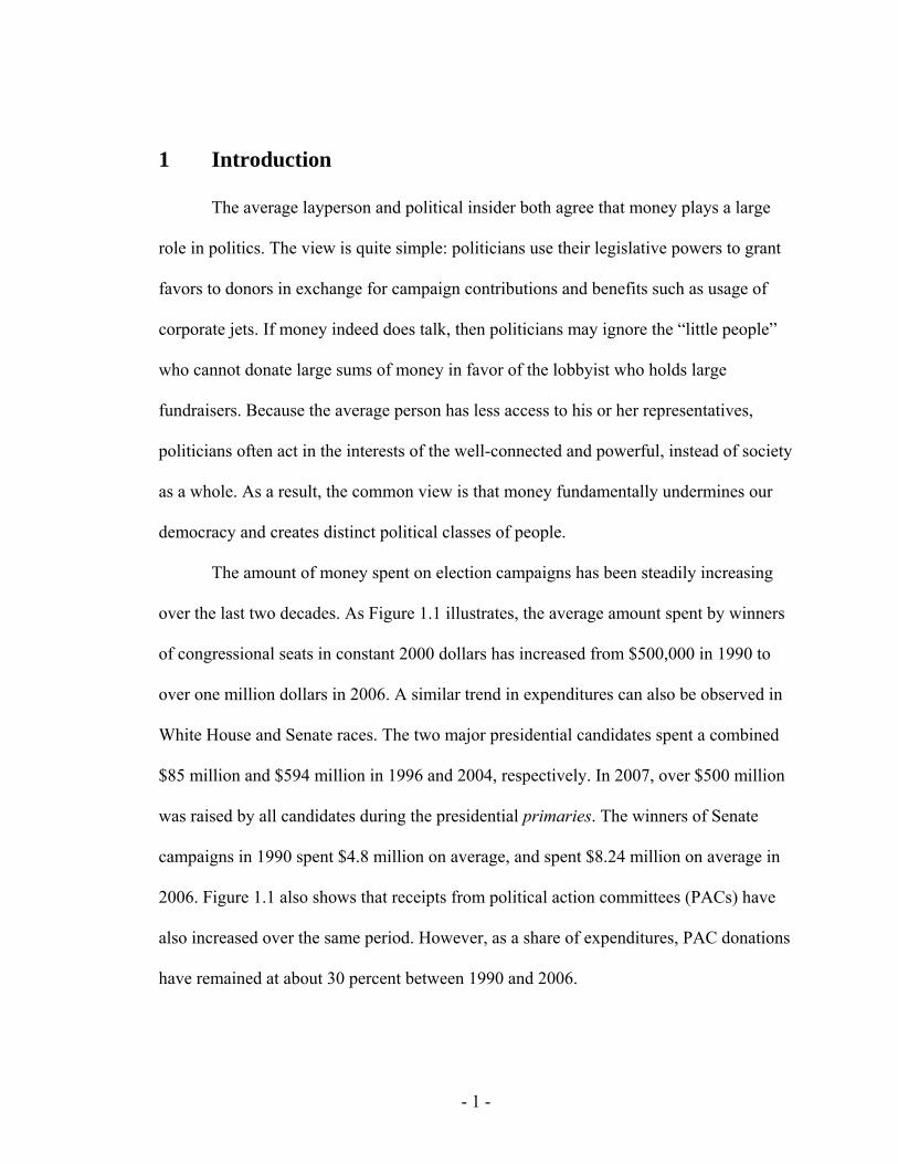
The amount of money spent on election campaigns has been steadily increasing

over the last two decades. As Figure 1.1 illustrates, the average amount spent by winners

of congressional seats in constant 2000 dollars has increased from $500,000 in 1990 to

over one million dollars in 2006. A similar trend in expenditures can also be observed in

White House and Senate races. The two major presidential candidates spent a combined

$85 million and $594 million in 1996 and 2004, respectively. In 2007, over $500 million

was raised by all candidates during the presidential primaries. The winners of Senate

campaigns in 1990 spent $4.8 million on average, and spent $8.24 million on average in

2006. Figure 1.1 also shows that receipts from political action committees (PACs) have

also increased over the same period. However, as a share of expenditures, PAC donations

have remained at about 30 percent between 1990 and 2006.

- 2 -

1.1 Background

Money has always been part of politics, but it was only after the enactment of the

Federal Election Campaign Act (FECA) in 1971 that disclosure of campaign

contributions became mandatory. In 1974, amendments to FECA created the Federal

Election Commission (FEC) and limited donations. Under FECA rules, individuals could

donate up to $2,000 to any candidate per election cycle, $20,000 to any national party

committee, and $5,000 to any PAC, but not to exceed $25,000 in aggregate per year. 1

In 2002, Congress signed the Bipartisan Campaign Reform Act (BRAC) hoping

to eliminate unlimited sums of “soft money.” Prior to its passage, national party

committees and other political organizations were allowed to use unregulated monies to

engage in unregulated “issue advertising.” Although explicit requests to vote for or vote

against a candidate were not made, the purpose of the advertisements was obvious.

BRAC also increased the limit on “hard money” (the amount individuals were allowed to

contribute to any candidate) to $2,300 per election cycle with adjustments for inflation.

While the research on the role of money and special interest groups in politics is

vast, the focus of this thesis will be on the influence of campaign contributions on

legislative voting. Because the legislative process is complicated, special interest groups

often play an important, but easily obfuscated role. I will examine how contributions

from agricultural groups affected voting on four amendments in the 1996 Farm Bill. I

have chosen the Farm Bill as a case study, because the benefits are concentrated on a

small group and the costs are spread throughout the public. Olson (1965) theorized that

the most powerful interest groups are relatively small, because it is easier to overcome

the free rider problem in coordinating collective action. This thesis will only address the 1 Primary and general elections count as separate cycles.

- 3 -

influence of contributions on voting behavior. To the extent that contributions influence

other legislative activities, such as the drafting of legislation, this thesis will not address

those possibilities.

This thesis is structured as follows: Section 2 presents a theoretical model of

campaign contributions and legislative voting, Section 3 reviews the relevant literature on

the influence of contributions on voting, Section 4 presents the empirical results on

voting on the 1996 Farm Bill, and the final section concludes this paper.

Figure 1.1. Average Amount Spent to Win House Race

0

200

400

600

800

1000

1200

1990 1992 1994 1996 1998 2000 2002 2004 2006

Year

Thou

sand

s of

Dol

lars

(2

000

Con

stan

t $)

Expenditures Receipts from PACs

Source: The Center for Responsive Politics, 2008.

2 Theory

While recognizing the importance of government involvement in the economy,

economists have traditionally avoided modeling government behavior. However, the field

of political economy has been gaining interest as economists have formulated new

theories on how government functions.

- 4 -

2.1 Economic Models of Voting

The standard premise in economic voting models is that political actors act in a

manner to maximize their utility. In the case of legislators in a representative system, it is

assumed that their most important goal is to win elections, because holding political

office gives the politician power. This model of the rational, utility maximizing political

agent comes from Duncan Black (1948) and Anthony Downs (1957). In this model,

which is traditionally known as the Downsian model, politicians serve the public interest,

even though they are self-interested. If candidates wish to win elections, they are subject

to the will of the people. Adam Smith’s invisible hand is applicable to the political arena.

2.1.1 Median Voter Theorem in a Representative Government

The Downsian model of political behavior is a spin-off of Hotelling’s linear city

model. The simple Downsian model predicts that candidates’ platforms will converge to

the median voter’s preferences. Figure 2.1 shows the frequency distribution of voters’

preferences if the frequency distribution is unimodal and symmetric. The median voter

holds position M. Assuming every voter votes, a candidate choosing position L will

obtain all the votes of voters holding positions to the left of position A, the midpoint of L

and R. The candidate choosing R will receive all the votes to the right of position A and

win the election. Knowing this, the candidate choosing L will shift his position to the

right to gain more votes. Similarly, the other candidate will shift towards the left to gain

more votes. The equilibrium is reached when both candidates hold position M, and the

equilibrium position matches the preferences of the median voter.2

2 If the frequency distribution is not unimodal and symmetric, Figure 2.1 will look different. In equilibrium, both candidates will still choose the platform of the median voter, but this position will no longer be the “mean” platform.

- 5 -

Figure 2.1. Frequency Distribution of Voters’ Preferences

Source: Mueller, Public Choice, 2003.

2.1.2 Probabilistic Voting3

More sophisticated models of probabilistic voting have been developed to correct

for the simplicities of the Downsian model, but the models, of course, still assume that

politicians attempt to win elections. A candidate’s vote total depends on his platform, θA,

and his opponent’s platform, θB. Most models also assume that voters are not fully

informed and can be influenced by campaign expenditures. It is assumed that campaign

contributions only serve the purpose of financing campaign expenditures and cannot be

embezzled. Therefore, contributions will be used synonymously with expenditures. Most

models also assume that because voters are not fully informed, expenditures by both

candidates, CA and CB, influence election results by informing voters of the candidate’s

platforms, reducing voter uncertainty, advertising certain qualities of the candidate or

discrediting the opposing candidate. The probabilities of winning an election for

candidates A and B therefore are

3 Model adopted from Mueller (2003).

- 6 -

( , , , )A A A B A BC Cπ π θ θ= and (2.1)

( , , , )B B A B A BC Cπ π θ θ= (2.2)

Because it is expected that own expenditures increase the expected vote total and

opponent expenditures do not, we have / 0A AEV C∂ ∂ > and / 0A BEV C∂ ∂ ≤ , where AEV

is candidate A’s expected vote total. If this were not the case, there would be no incentive

for candidates to request donations or hold fundraisers.

When making the decision to donate money, contributor i considers the utility he

receives from the winner’s platform and his consumption of private goods, vi. Assuming

diminishing marginal utility from consumption of private goods, his utility function is

( , )i i iU U vθ= , with 0i

i

Uv

∂>

∂ and

2

2 0i

i

Uv

∂<

∂.

For the moment, we will assume that contributions do not influence candidates’

platforms and that contributions only influence the probability of a candidate’s victory.

Then contributor i’s expected utility can be written as

( ) ( , ) (1 ) ( , )i A i A i A i B iE U U v U vπ θ π θ= + − (2.3)

Let us assume that i i iy v C= + is contributor i’s budget constraint, where yi is the

contributor’s income. The value of private goods consumed and contributions given

cannot exceed his income. His objective function is

( ) ( , ) (1 ) ( , ) ( )i A i A i A i B i i i iE U U v U v y v Cπ θ π θ λ= + − + − − , (2.4)

where πA is the probability of candidate A winning the election. Assuming the contributor

only gives to one candidate (here, candidate A), maximizing the objective function with

respect to CA and vi leads to

- 7 -

( ) ( , ) ( , ) 0i A Ai A i i B i

A A A

E U U v U vC C C

π πθ θ λ∂ ∂ ∂= − − =

∂ ∂ ∂, and (2.5)

( ) ( , ) ( , )(1 ) 0i i A i i B iA A

i i i

E U U v U vv v v

θ θπ π λ∂ ∂ ∂= + − − =

∂ ∂ ∂. (2.6)

If ( , ) / ( , ) /i A i i i B i iU v v U v vθ θ∂ ∂ = ∂ ∂ , then first order maximization of the objective

function yields

( , )[ ( , ) ( , )]A i A ii A i i B i

A i

U vU v U vC vπ θθ θ∂ ∂

− =∂ ∂

. (2.7)

The right hand side of the equation (2.7) is the marginal utility of consuming an

additional unit of a private good. If the contributor prefers one candidate’s platform over

the other’s, e.g. ( , ) ( , )i A i i B iU v U vθ θ> , then the equation has a solution with CA > 0. The

contributor would not donate money to candidate B since any contribution would increase

B’s probability of winning.4 We see this behavior when conservative groups contribute to

conservative candidates, and liberal groups contribute to liberal candidates. With

candidates’ platforms held fixed, the contributor will only give to the candidate whose

platform provides the most utility, contributing to the candidate up to the point where the

increase in expected utility from the increase in the probability of his preferred candidate

winning equals the reduction in utility from the decrease of his consumption of private

goods.

When the candidates choose their platforms, they are aware that their choice will

influence both his own and his opponent’s campaign contributions, i.e. ( , )A A A BC C θ θ=

4 However, in the real world, contributors have been known to give small amounts to their preferred candidate’s opponent to deter any controversy involving the contributors’ donations. In the theoretical model, we assume the gap in donations between the two candidates is large, so we assume one candidate receives no contributions without loss of generality. Theoretically, a contributor may also give to two candidates if the contribution can move both candidates’ platforms towards the one preferred by the contributor.

- 8 -

and ( , )B B A BC C θ θ= . If θB remains fixed, candidate A chooses θA to maximize his

probability of winning the election (πA):

A A A A B

A A A B A

C CC Cπ π π

θ θ θ∂ ∂ ∂ ∂ ∂

= − −∂ ∂ ∂ ∂ ∂

(2.8)

If we assume that contributions not only affect the probability of winning, but also

the platforms of the candidates, i.e. ( , )A A A BC Cθ θ= and ( , )B B A BC Cθ θ= , then the

probability of candidate A winning is [ ( , ), ( , ), , ]A A A A B B A B A BC C C C C Cπ π θ θ= and the

contributor’s utility function can be expressed as [ ( , ), ]i i A A B iU U C C vθ= or

[ ( , ), ]i i B A B iU U C C vθ= depending on whether A or B wins the election. It is assumed that

contributions to a candidate will shift the candidate’s platform towards the one preferred

by the contributor. A contributor would not contribute to a candidate if the contribution

causes the candidate to move farther away from his ideal platform.

Without the influence of campaign contributions, both candidates would follow

the Downsian model of voting, where candidates choose the platform preferred by the

median voter. Under these circumstances, choosing the median platform is the unique

Nash equilibrium and the candidates will split the vote evenly. However, when campaign

expenditures are included in the model, candidates may gain more votes by accepting

contributions. However, accepting contributions is not without cost: in order to attract

contributions, the candidate must choose a platform different than the median voter’s

preferred platform. Therefore, the vote-maximizing candidate will accept contributions

up to the point where the increased probability of winning an election caused by an

increase in campaign contributions is equal to the decreased probability of losing the

election caused by shifting his platform away from the median voter. Candidates choose

- 9 -

their platforms with these considerations in mind and balance the interests of their

contributors and constituents. Thus, money affects both the platforms and probabilities of

victory for each candidate.

While this thesis will not test the effect of contributions on election outcomes, it

will add to the literature on contributions and legislative voting behavior. This thesis

directly tests the influence of campaign contributions on voting on the 1996 Farm Bill.

3 Literature Review While theoretical models of voting suggest that campaign contributions may

influence voting behavior, their complexity suggests that finding empirical evidence may

be difficult. Indeed, empirical studies have produced mixed results. Much of the literature

attempts to address the possibility that contributions are endogenous with respect to

legislative voting behavior (Welch 1981, Kau Keenan and Rubin 1982). Legislators often

support a special interest group’s interests regardless of whether or not they receive any

contributions. For example, legislators from a farming state will vote in favor of farming

subsidies even if they did not receive any contributions from farming groups, because

farming subsidies would benefit their constituents. If a group contributes to the candidate

and the candidate supports the group’s interests, then a single equation model would

overstate the causal relationship between contributions and legislative voting behavior.

Hence, empirical models of roll call behavior should also estimate contribution functions

and control for variables that might influence both voting and contributing.

Roscoe and Jenkins (2005) conduct a meta-analysis of over 30 studies looking at

the impact of contributions on roll call voting and found that different empirical

- 10 -

specifications have an impact on whether significant results are present. Of the 357

coefficients on contributions in their survey, 35.9 percent were significant at the 0.05

level. The inclusion of legislator ideology variables reduces the likelihood of finding a

significant relationship, but the inclusion of constituency variables has no effect.

Specifications using simultaneous equations, which are typically considered to be more

precise than single equation methods, appear to have no effect on whether significant

values are present.

Roscoe and Jenkins argue that contribution variables from competing groups

often are not specified properly. As a result, they find that the inclusion of multiple

contribution variables reduces the probability of finding a significant relationship. They

argue that this phenomenon is likely caused by multicollinearity between contributions

from competing interest groups. For example, labor groups are less likely to contribute to

legislators who receive large contributions from corporate groups. Roscoe and Jenkins

argue that a better way of specifying contributions from competing groups would be to

subtract one group’s contributions from the other group’s contributions. However, by

taking the net contributions, they are restricting the coefficients of both variables to be

equal to each other. This can be seen from equations (3.1) and (3.2).

1 2 1 3 2 1iy C Cα α α ε= + + + (3.1)

1 2 1 2 2( )iy C Cβ β ε= + − + (3.2)

where yi is the vote of legislator i and C1 and C2 are contributions from two competing

interest groups. Equation (3.1) allows for the possibility that C1 and C2 may have

different coefficient estimates. By specifying the vote equation as a function of the net

- 11 -

contributions received as in equation (3.2), the model is in effect restricting β2 = α2 - α3.

Yet, there is no reason to expect this assumption to be true.

Ansolabehere, de Figuieredo and Snyder (2003) survey nearly 40 papers in the

economics and political science literature that examine the relationship between

campaign contributions and congressional voting records, and find a statistically

significant impact in only one quarter of the papers surveyed. However, many of the

papers surveyed omit crucial variables and do not address the likely endogeneity between

contributions and voting. In addition to their survey of the literature, the authors also use

instrumental variables regression and control for member or district fixed effects in their

estimation models. They do not find any detectable effects on legislative behavior.

One of the first empirical models to consider the endogeneity of campaign

contributions was proposed by Chappell (1981, 1982). His “Simultaneous Probit-Tobit

(SPT) Model” is presented as follows:

1

*2 1 1 1i i i iy y Xγ β ε= + + (3.3)

2

*2 2 2 2i i iy Xβ ε σ= + (3.4)

1

*1

1 *

1 if 00 if 0

i

ii

yy

y⎧ >⎪= ⎨ ≤⎪⎩

(3.5)

* *2 2

2 *2

if 00 if 0

i ii

i

y yy

y⎧ >

= ⎨≤⎩

(3.6)

where *

1iy = a dependent variable indicating the net benefit legislator i receives from voting for a piece of legislation;

*2iy = a dependent variable indicating the contributions made to candidate i;

1iy = a dummy variable equal to 1 if the vote is “yes” and 0 if the vote is “no”;

2iy = the actual contribution from the interest group to legislator i;

- 12 -

X1i = a vector of variables indicating constituency characteristics and the fixed attribute of legislator i; X2i = a vector of variables indicating the legislative power of legislator i if he is elected, his probability of election, and his initial position on the issue; and ε1, ε 2 are random error terms. The assumptions on the error terms are E(ε ji) = 0; E(ε ji

2) = 1; E(ε 1i, ε 2i) = ρ (3.7) Equation (3.3) estimates the likelihood that a congressman votes “yes” or “no” on

a particular bill. Since the voting variable is dichotomous, OLS estimates result in

heteroskedastic standard errors. By using a linear probability model, the assumption is

that the marginal effect of every donation is constant. An even more serious problem

occurs when estimating a dichotomous variable with OLS: it is possible to obtain

predicted probabilities less than zero or greater than one.

As a result, a nonlinear Probit (or Logit) model is the appropriate tool of analysis.

In a Probit model, *1iy is a latent variable indicating the net benefit the congressman

obtains from voting on a particular piece of legislation. It also serves as an index

measuring the legislator’s propensity to vote in favor of the legislation. Equation (3.5)

assumes that if the net benefit from voting for the piece of legislation is positive, i.e.

*1 0iy > , then the legislator would vote for the legislation. If *

1 0iy ≤ , then the legislator

would vote against it. The coefficient, γ, indicates whether contributions have a positive

or negative effect on voting “yes.” X1i includes variables such as constituents’ economic

interests and the legislator’s ideology and party.

Similarly, *2iy represents the interest group’s propensity to contribute to a

candidate. Since contributions cannot be negative, applying the standard OLS estimation

technique can lead to biased estimates. A Tobit model is used to estimate the contribution

- 13 -

equation (3.4). It is assumed that groups only contribute to candidates when the net

benefit of contributing is positive. X2i is a set of variables that would influence

contribution behavior. X1i is generally a subset of X2i. Other variables in X2i include the

legislative power of the congressman (membership of powerful committees, tenure, etc.)

and the margin of victory in the previous election. If interest groups want to influence the

legislative agenda, they should donate to legislators with more power. If interest groups

want to help elect friendly legislators, they may donate more money when their favored

legislator is facing a close election.

The set of equations in (3.7) outline the necessary conditions on the error terms in

the model. The vote and contribution equations can be estimated consistently with single

equation methods if the error terms in the equations are uncorrelated. However, if an

unobserved component that influences both equations is omitted, then the error term in

voting equation would be correlated with the explanatory variables. Estimation of the

model would result in biased and inconsistent parameters. For example, members of a

logrolling coalition are more likely to vote in favor of a contributor’s interests and more

likely to receive contributions. As members of a logrolling coalition, the legislators

would have voted for the contributor’s interests, regardless of the amount of contributions

received.

The difference between Chappell’s SPT model and normal Probit-Tobit models is

that Chappell allows for a non-zero correlation between the error terms of the voting and

contribution equations. Chappell’s model uses FIML estimation methods to overcome the

problem with the single equation estimation procedure.

- 14 -

Using this model, Chappell found that contributions had a positive impact on

voting in six of seven votes studied, but only one vote had a marginally significant

coefficient. Disappointed with his results, he suggested that better models of

contributions and voting behavior might result in greater precision.

Stratmann (1991) disagreed with Chappell’s assessment that the empirical model

was flawed. Instead he claimed that narrower issues with gains concentrated among small

groups and losses spread throughout the electorate would be more ideal to study. Using

Chappell’s model, Stratmann looked at the influence of campaign contributions on the

1985 Farm Bill and found contributions to have a statistically significant impact on eight

out of ten votes. Stratmann estimated that a $3,000 contribution from sugar groups would

have resulted in a virtually certain pro-sugar vote. In addition, Stratmann predicted that a

pro-sugar amendment would have failed 203-210, instead of passing 267-146, in the

absence of any contributions from sugar interests. In four of the ten votes studied,

Stratmann rejected the null hypothesis that the error terms of the voting and contributions

equations were not correlated, suggesting that contributors gave money to congressmen

who were already likely to support their cause.

Other studies have extended Chappell’s SPT model to include contributions from

competing groups. Brooks, Cameron, and Carter (1998) found pro-sugar and anti-sugar

contributions to have significant and anticipated signs in five of six cases. Magee (2002)

studied voting on NAFTA, family leave, abortion, defense spending and gun control, and

found contributions to be significant only in the case of defense spending. These results

may not be surprising if one believes that defense spending is less ideological and less

prominent than the other issues studied. Baldwin and Magee (2000) found labor and

- 15 -

corporate contributions to have a significant effect on NAFTA and the GATT Uruguay

Round bill. They estimate that labor contributions bought 67 votes against NAFTA and

57 votes against the GATT bill, while corporate contributions bought 41 votes for

NAFTA and 35 votes for the GATT bill. Wolaver and Magee (2006) study the effects of

contributions from law firms, insurance groups and health care groups on a bill capping

noneconomic damages in medical liability lawsuits. They found that contributions from

law firms decreased the probability of voting in favor of the legislation, while

contributions from insurance and health care groups increased the probability of voting

for the legislation.

The influence of special interest groups on farming bills has also been extensively

researched. Welch (1982) found evidence of reciprocity between congressmen and milk

PACs. However, Abler (1991) found that pro-farm legislators attract more contributions,

but contributions do not buy the votes of legislators. Brooks (1997) found that

contributions to House members were influential in voting on limiting farm payments,

but contributions to senators were not. Ellison and Mullin (1995) surprisingly found that

large, unconcentrated groups, rather than wealthy and unconcentrated groups, were more

influential in lobbying on sugar tariff reform in 1912. Gawande (2006) found evidence of

lobbying influence on agricultural trade protection and subsidies.

This thesis will use Chappell’s empirical model to test the influence of voting on

four proposed amendments to the 1996 Farm Bill aimed at limiting subsidies. In addition,

it will also test the influence of competing interest groups on one particular amendment.

- 16 -

4 Empirical Analysis

Romantic notions of agrarian life have been a part of American culture since the

country’s founding. The vision of farmers working tirelessly under brutal conditions to

feed themselves and their fellow citizens invokes a sense of admiration from many

Americans. In the early days of the nation, many people believed that the status of

farmers and the condition of the nation were irrevocably linked. In an address to

Congress in 1796, George Washington stated, “It will not be doubted that with reference

either to individual or national welfare agriculture is of primary importance” (Wanlass,

2000).

Not surprisingly, the government has a long history of promoting agrarian life.

The Homestead Act of 1862 allowed anyone who did not take up arms against the

government to file for 160 acres of unoccupied land. The land officially became the

homesteader’s property after five years, provided he make improvements on the land.

Another way the government encouraged farming was through the improvement of rural

infrastructure. Extensive investment in irrigation systems, drainage systems, and large

dams in the 19th and early 20th centuries acted as a generous subsidy to western farmers.

Other government-led initiatives, such as collection of market information and support

for agricultural research, decreased farmers’ risks and increased their productivity.

While government support of farming has long been a tradition in America, it was

only relatively recently that the federal government directly regulating commodity

programs. After commodity prices plunged in the early 1920’s, various proposals for

stabilizing prices were debated in Congress. The Agricultural Marketing Act of 1929

marked the first major intervention in commodity prices. It established the Federal Farm

- 17 -

Board, which bought 250 million bushels of wheat in 1930 in an effort to support wheat

prices. However, its attempts ultimately failed due to worldwide deflation. Passed in

1933, the landmark Agricultural Adjustment Act attempted to manage the supply of

livestock and crops by making payments to farmers who took supply-limiting actions,

such as delivering livestock for slaughter, idling land and even destroying planted crops.

Various supply management policies remain in effect to this day. In 2000, contracts with

the Conservation Reserve Program resulted in 36 million acres, or eight percent of all U.S.

cropland, remaining idled.5 Farm Bills, which are passed approximately every five years,

reauthorize programs dating back to the 1930’s and occasionally authorize new programs.

The federal government has also pursued more controversial policies in directly

supporting farmers’ incomes. Favorable borrowing programs allow farmers to take out

loans and pledge their crops as collateral. Other methods to support farmers’ incomes

include direct payments to farmers during periods of depressed prices, import quotas and

tariffs on foreign crops and livestock, and export subsidies to help expand farmers’

markets.

However, cost-benefit analyses have usually shown that commodity programs are

not worthwhile. The GAO (2000) estimates that import tariffs on sugar transfer $1.1

billion to sugar and corn sweetener producers at a cost of $1.7 billion to sugar buyers.

Gardner (2002) estimates the cost of idling 30 million acres under grain programs in the

1980’s was $1.5 billion annually. Table 4.1 presents estimates of the costs and benefits of

various commodity programs in 1987.

5 For more in-depth information on the history of government involvement in agriculture, see Gardner (2000).

- 18 -

Table 4.1 (Section 4, Table 1): Gains to producers, consumers, and taxpayers from commodity programs (billions of dollars, 1987 fiscal year)

Commodity Producers Consumers Taxpayers Feed Grains 8.9 0 -10.3

Wheat 2.4 0 -3.7 Rice 0.5 0 -0.6

Cotton 0.9 0 -1.5 Sugar 2.7 -3.1 0 Milk 1.3 -1.2 -1.4

Tobacco, Peanuts and Wool 0.8 -0.5 -0.2 Total 17.5 -4.8 -17.7

Source: Garder, 2002, p. 239

4.1 The 1996 Farm Bill

In response to growing criticism of the commodity programs, Congress enacted

the Agricultural Market Transition Act (HR 2854) in 1996 to fundamentally reform

subsidies for commodities. The debate split legislators along regional and party lines.

Democrats and Republicans from farming states united to preserve subsidies for crops

produced by their constituents. The intention of the bill, also known as the “Freedom to

Farm Bill,” was to gradually eliminate subsidies for most crops and, as noted in its

official name, help farmers transition from a government regulated market to a free

market. The main provision of the bill authorized fixed, declining federal payments to

farmers. Supporters of the bill had hoped that farmers would rotate crop production in

accordance to changing market conditions, instead of relying on government payments.

Since these payments were fixed, farmers would not have been given supplemental

payments if commodity prices dropped.6 President Clinton signed the bill into law on

April 4, despite reservations that farmers might lose a safety net.

6 However, when commodity prices fell in the late 1990’s, Congress appropriated $7.9 billion in emergency payments. The 2002 Farm Bill also reversed some of the reforms from the 1996 Farm Bill.

- 19 -

4.2 Description of the Variables

The House considered four amendments to limit further crop subsidies. The

amendments, H.AMDT 932, H.AMDT 933, H.AMDT 934 and H.AMDT 935, attempted

to phase out price support programs and marketing assistance loans for cotton, peanuts,

sugar and dairy products. As Table 4.2 shows, partisan ideologies did not play a large

role in the voting. Figures 4.1 to 4.4 show that regional interests were relevant.

Table 4.2 (Section 4, Table 2) Roll Call by Party Cotton

Amendment Peanut

Amendment Sugar

Amendment Dairy

Amendment Votes in Favor of

Amendment 65 D 102 R

84 D 125 R

75 D 133 R

109 D 149 R

Votes Against Amendment

122 D 130 R

1 I

103 D 108 R

1 I

114 D 102 R

1 I

78 D 85 R 1 I

Total 167-253 209-212 208-217 258-164 Note: D = Democrat, R = Republican, I = Independent

Figure 4.1. Cotton Vote by Region

Figure 4.2. Peanut Vote by Region

- 20 -

Figure 4.3. Sugar Vote by Region

Figure 4.4. Dairy Vote by Region

Cotton escaped the reforms originally introduced in the Farm Bill, but

Representative Steve Chabot (OH-R) introduced amendment H.AMDT 932 to include

cotton subsidies. Chabot’s amendment would have eliminated marketing assistance loans

and loan deficiency payments for cotton growers after 1998. By helping farmers maintain

a stable level of income, marketing assistance loans and loan deficiency payments act as

income subsidies. Marketing assistance loans allow farmers to pledge their crops as

collateral and store their crops when market conditions are unfavorable. If conditions

improve, farmers can sell their stored crops and repay the loan. On the other hand, if

conditions stagnate or worsen, farmers are allowed to keep the loan and give up their less

valuable collateral. Loan deficiency payments work in a similar manner. Chabot’s

amendment failed 167-253 and cotton subsidies remained.

- 21 -

Rep. Christopher Shays (R-Conn.) introduced H.AMDT 933 in an attempt to

phase out the peanut support program over a seven year period. The decades-old program

relied on a combination of government loans and production limits to maintain minimum

peanut prices. Southern legislators, claiming that elimination of the program would

devastate small farmers and rural areas, fought vigorously to save the program. After the

vote was tallied, the amendment to phase out price supports for peanuts was ultimately

defeated 209-212, giving a victory to Southern legislators and peanut growers.

H.AMDT 934 followed the peanut vote, and according to Congressional

Quarterly, was even more anticipated. Over the course of 1995, sugar interests lobbied

against manufacturing, consumer, and environmental groups to maintain sugar subsidies

in the Farm Bill. Rep. Dan Miller (R-Fl.), a frequent critic of the sugar support program,

introduced the amendment to phase out the sugar price support program over five years.7

Opponents of the amendment contended that the proposed Farm Bill had already reduced

subsidies for sugar and that Miller’s amendment would lead to job loss and dependency

on foreign sugar. The amendment was defeated 208-217.

The immediate elimination of many subsidies for dairy was initially part of the

Farm Bill’s agenda, but Rep. Gerald Solomon (R-NY) proposed an amendment to extend

price supports for butter, powdered milk, and cheese for five years. However, the most

controversial provision in H.AMDT 934 was the restoration of dairy marketing orders

that were eliminated in the proposed Farm Bill. Marketing orders, established in 1937,

determine the amount of money that producers of cheese, ice cream, and powdered milk

must pay farmers for their milk. The price, which varies in different parts of the country,

7 Rep. Miller and other legislators opposed to sugar subsidies make regular attempts to attach anti-subsidy amendments to legislation.

- 22 -

is based on a formula that takes into account how far a farmer lives from Wisconsin. The

system’s stated purpose is to encourage milk production outside the Upper Midwest and

to guarantee that unspoiled milk would be available throughout the country. Without

marketing orders, dairy farmers in the Northeast would face lower milk prices, and many

would likely be forced out of the market. Solomon’s amendment to restore marketing

orders would have benefited Northeastern dairy farmers at the expense of Midwestern

dairy farmers. Not surprisingly, the dairy lobby was divided on the proposed amendment

along regional lines. Despite protests from Midwestern legislators, the amendment to

restore marketing orders was anticlimactically adopted 258-164.

The votes for each amendment have been coded so that “one” represents a pro-

subsidy position and “zero” represents an anti-subsidy position. For example, a vote in

favor of phasing out subsidies for peanuts is recorded as “zero,” and a vote against

phasing out subsidies for peanuts is recorded as “one.” In the case of the dairy

amendment, opposition to the amendment was coded as “zero,” while support was coded

as “one.”

Data on contributions from the 1995-1996 campaign cycle were compiled from

FEC filing reports available on the FEC web site. Contributions from members of each

respective interest group were added together to create an aggregate contribution

variable.8 For example, contributing members of the sugar lobby include Flo-Sun Inc,

American Crystal Sugar, United States Sugar Corporation, and the American Sugarbeet

Growers Association. Although every effort was made to identify all interested groups, it

is inevitable that some of the more obscure groups have been overlooked. A priori, the

expected coefficient of the contributions variable should be positive. For the dairy 8 See Appendix B for list of all interest groups included in analysis.

- 23 -

amendment, since the dairy industry was divided over the amendment, the contributions

from dairy groups have been divided into the anti-marketing orders group and pro-

marketing orders group.9

Table 4.3 shows that sugar groups were the most generous donors with average

donations of $4,200 per legislator. Among the legislators who received any contributions,

the average was over $5,500. Cotton and peanut groups averaged less than one thousand

dollars per legislator, but when considering only contributions greater than zero, cotton

and peanut groups average $1,800 and $2,600 per contribution, respectively. The average

contribution from anti-marketing orders dairy groups was $1,800, while the average

contribution from pro-marketing orders dairy groups was just over one thousand dollars.

Table 4.3 (Section 4, Table 3). Average Contribution by Industry (Thousands of Dollars)

Cotton Peanut Sugar Dairy Contributions

Against Amendment 0.483 / 1.812 0.887 / 2.649 4.200 / 5.579 1.8058 / 2.9423

Contributions in Favor of Amendment - - - 1.0684 /

2.0128 Note: The first number is the average contribution. The second number is the average contribution given contribution > 0.

Since legislators also consider the interests of their constituents, the relative

importance of agriculture in each district is a factor in legislators’ voting decisions.

Legislators from districts with farming interests should be more inclined to vote for in

favor of preserving subsidies. Depending on the vote taken, the number of farms

represents the number of cotton, peanut, sugar beet, sugarcane, or dairy farms in a

9 Groups were identified either through stated positions on the issue or location of the main headquarters of the group. Groups from the Midwest were assumed to be against marketing orders, while groups outside the Midwest were assumed to be in favor of marketing orders.

- 24 -

district.10 The 1990 Census recorded the total number of farms producing each crop for

the 103rd Congress. The 103rd Congress remained in effect throughout the decade, except

when a state initiative or court-ordered redistricting was enacted. Six states redistricted

during the 104th Congress: Georgia, Louisiana, Maine, Minnesota, South Carolina, and

Virginia. For these states, the mapping software, ArcGIS, was used to roughly distribute

farms from the 103rd congressional district boundaries to the 104th congressional district

boundaries.

Figures 4.5 to 4.8 show the distribution of cotton, peanut, sugar and dairy farms.

Cotton and peanuts are grown almost exclusively in the South. Sugar beet farms are most

often located in the West and Midwest in states such as California and Minnesota.

However, sugarcane production requires a tropical climate and as a result, only occurs in

California, Hawaii, Louisiana and Texas. Dairy is produced throughout the country with

a large concentration in the Midwest.

Figure 4.5. Distribution of Cotton Farms in the U.S.

10 A sort of robustness check for the number of farms is the level of agricultural production. Crop production data was obtained from the Agricultural Statistics Database of the USDA's National Agricultural Statistics Service. Annual county level data for each crop production were reported in terms of harvest (acres) and production (tons). Regressions with harvest and production data are included in Appendix D. In cases where a county lay between multiple districts, harvest/production data were distributed proportionally with respect to land area and inversely proportionally with respect to population according to this formula: 1 1 1

12 1 2

County Subdivision Population County Subdivision Land Area

Total County Population Number of Subcounty Divisions Total County Land Area− +

−

⎛ ⎞⎛ ⎞ ⎛ ⎞⎜ ⎟⎜ ⎟ ⎜ ⎟⎝ ⎠⎝ ⎠ ⎝ ⎠

The rationale behind this approach is that farming is more common in areas with less population density.

- 25 -

Figure 4.6 Distribution of Peanut Farms in the U.S

Figure 4.7. Distribution of Sugar Beet and Sugarcane Farms in the U.S.

Figure 4.8. Distribution of Dairy Farms in the U.S.

- 26 -

A dummy variable representing the party of the legislator is included in the voting

equation.11 The variable has been coded so that a Republican is “one” and Democratic is

“zero.” Republicans were in control of the 104th Congress with 230 members, while

Democrats held 204 seats. The one independent, Rep. Bernie Sanders (VT at-large),

caucused with Democrats. For the purposes of this paper, he is treated as a Democrat

because of his liberal views. At the time of the voting on the Farm Bill, five

congressional seats were vacant.12

As a measure of a representative's ideology, ratings from the American

Conservative Union were included in the analysis. The rating measures each

representative’s conservative tendencies on a scale from zero to one-hundred. The 1996

ratings were derived from votes that the ACU regarded as key votes in 1996. Not

surprisingly, since the Congress was under Republican control, the average congressman

had a slightly above average ACU rating of 56.

Dummy variables indicating the legislator’s geographic region were also included

since many of the amendments had regional interests. For example, Southern legislators

fought to save subsidies for peanuts and cotton. Midwestern legislators were opposed to

restoring marketing orders for dairy.

For the Tobit equation modeling contributions, the margin of victory variable

denotes each representative’s share of the popular vote in 1994. If interest groups wish to

maximize the effect of their contributions, they may donate more to candidates involved

11 Five representatives switched from the Democratic Party to the Republican Party during the period. They were Nathan Deal (Georgia 9th), Billy Tauzin (Louisiana 3rd), Jimmy Hayes (Louisiana 7th), Mike Parker (Mississippi 4th), and Gregory Laughlin (Texas 14th). 12 Rep. Norman Mineta (D-California 15th) resigned midterm to accept a position at Lockheed Martin. Rep. Kweisi Mfume (D-MD 7th) resigned to become president of the NAACP. Rep. Ron Wyden (D-OR 3rd ) won a special election for Oregon senator. Reps. Walter R. Tucker (D-CA 37th) and Mel Reynolds (D-IL 2nd) resigned amid scandals.

- 27 -

in close elections to influence the outcome. As a result, the expected sign of the margin

variable in the contributions equation is negative. Candidates running unopposed were

given one-hundred percent of the vote.

Two other variables in the contribution equation are membership on the House

Agricultural Committee and membership on House Appropriations Committee. The

Agricultural Committee is responsible for drafting the basic framework of the legislation

before it is voted upon by the rest of the House. The Appropriations Committee decides

the annual expenditures for farm programs. Since membership in either of these

committees confers a great deal of power to legislators, the coefficients for these

variables in the contributions equations are expected to be positive.

Table 4.4 (Section 4, Table 4) Summary Statistics for the 104th Congress

VARIABLE Definition Mean Std. Dev. Min. Max.

PARTY Democrat = 0 Republican = 1 0.552 0.498 0 1

ACU 0 = Most Liberal 100 = Most Conservative 56.355 40.644 0 100

SOUTH Dummy variable: South = 1 0.3402 0.4743 0 1

MIDWEST Dummy variable: Midwest = 1 0.2345 0.4242 0 1

APPROP Dummy variable: Membership on Appropriations Committee = 1 0.1333 0.3403 0 1

AG Dummy variable: Membership on the Agricultural Committee = 1 0.1149 0.3193 0 1

MARGIN Share of Popular Vote in 1994 64.739 13.417 42.557 100

Table 4.5 (Section 4, Table 5) Summary Statistics for the Cotton Amendment (N=420)

VARIABLE Definition Mean Std. Dev Min. Max.

VOTE 1 = Pro-subidy 0 = Anti-subsidy 0.602 0.490 0 1

CONTRIBUTION Thousands of Dollars 0.483 1.342 0 10.5

FARM Hundreds of farms 0.7496 2.88805 0 26.21

HARVEST Thousands of acres 34.384 148.428 0 1,680.555

PRODUCTION Thousands of tons 37.619 152.888 0 1,518.222

- 28 -

Table 4.6 (Section 4, Table 6): Summary Statistics for the Peanut Amendment (N=421)

VARIABLE Definition Mean Std. Dev Min. Max. VOTE 1 = Pro-subidy

0 = Anti-subsidy 0.504 0.501 0 1

CONTRIBUTION Thousands of Dollars 0.887 2.795 0 27.25 FARM Hundreds of farms 34.803 2.2124 0 25.97

HARVEST Thousands of acres 3.489 22.823 0 290.911 PRODUCTION Thousands of tons 7,959.1 54,127.2 0 782,926.9

Table 4.7 (Section 4, Table 7): Summary Statistics for the Sugar Amendment (N=425)

VOTE Definition Mean Std. Dev Min. Max. SUGAR 1 = Pro-subsidy

0 = Anti-subsidy 0.511 0.500 0 1

CONTRIBUTION Thousands of Dollars 4.200 5.355 0 46.9 FARM Hundreds of sugar beet

farms 0.207 1.16126 0 11.45

FARM_2 Hundreds of sugarcane farms

0.0203 0.23639 0 4.65

HARVEST Thousands of acres (sugar beet)

3.281 21.968 0 310.9

HARVEST_2 Thousands of acres (sugarcane)

2.057 15.929 0 199.453

PRODUCTION Thousands of tons (sugar beet)

64.427 420.734 0 5,793.3

PRODUCTION_2 Thousands of tons (sugarcane)

68.576 517.051 0 6,615.175

Table 4.8 (Section 4, Table 8): Summary Statistics for the Dairy Amendment (N=422)

VARIABLE Definition Mean Std. Dev Min. Max. VOTE 0 = Anti-marketing orders

1 = Pro-marketing orders 0.611 0.488 0 1

CONTRIBUTION Thousands of Dollars (Anti-marketing orders)

1.8058 2.7681 0

21.923

CONTRIBUTION_1 Thousands of Dollars (Pro-marketing orders)

1.0684 2.0920 0

20.95

FARM Hundreds of farms 230.341 5.15999 0 47.70 Note: Production data for dairy products was not included due to incompleteness of data.

- 29 -

4.3 The Empirical Model

To account for the possibility of endogenous contributions, I will utilize

Chappell’s Simultaneous Probit-Tobit Model as described in the previous Section.13 The

general model of legislator i’s vote on the cotton, peanut and sugar amendments is:

*1 1 2 3 4 5 1i i i i i i iVOTE CONTRIB FARM PARTY ACU SOUTHβ β β β β ε= + + + + + (4.1)

*1 2 3 4i i i i iCONTRIBUTION FARM PARTY ACU SOUTHγ γ γ γ= + + +

5 6 7 2 2i i i iAG APPROP MARGINγ γ γ ε σ+ + + + (4.2)

*

*

1 if 00 if 0

i

ii

VOTEVOTE

VOTE⎧ >⎪= ⎨ ≤⎪⎩

(4.3)

* *

*

if 0 0 if 0

i ii

i

CONTRIBUTION CONTRIBUTIONCONTRIBUTION

CONTRIBUTION⎧ >

= ⎨≤⎩

. (4.4)

For the dairy amendment where there were competing interest groups the model is:

*1 1 2 1 3_1

i i i iVOTE CONTRIBUTION CONTRIBUTION FARMβ β β= + +

4 5 6 1i i i iPARTY ACU MIDWESTβ β β ε+ + + + (4.5)

*1 2 3 4i i i i iCONTRIBUTION FARM PARTY ACU MIDWESTγ γ γ γ= + + +

5 6 7 2 2i i i iAG APPROP MARGINγ γ γ ε σ+ + + + (4.6)

*1 2 3 4_1

i i i i iCONTRIBUTION FARM PARTY ACU MIDWESTχ χ χ χ= + + +

5 6 7 3 3i i i iAG APPROP MARGINχ χ χ ε σ+ + + + (4.7)

* *

*

if 0 0 if 0

i ii

i


CONTRIBUTION⎧ >

= ⎨≤⎩

(4.8)

* *

*

_1 if _1 0_1

0 if _1 0i i

ii


CONTRIBUTION⎧ >

= ⎨≤⎩

(4.9)

13 Regressions with interaction variables are included in the Appendix D. Most interaction terms were not statistically significant, so they were dropped in the model.

- 30 -

The assumptions on the error terms are the same as in Chappell’s model:

E(ε ji) = 0; E(ε ji2) = 1; E(ε 1i, ε 2i) = ρ (4.10)

The model assumes that there are no omitted variables that influence voting and

contributions. As long as the correlation between the error terms does not equal zero, i.e.

ρ ≠ 0, then equations (4.1) and (4.5) can be estimated consistently with a single equation

Probit estimator.

The SPT model can be estimated using full information maximum likelihood

(FIML) methods.14 FIML estimates are consistent and asymptotically efficient. Using

FIML techniques overcomes the restriction that ρ ≠ 0, which is required for the model to

be estimated consistently with single equation models. FIML can also estimate the value

of ρ. The null hypothesis, ρ ≠ 0, is that there is no simultaneity between voting and

contributions. A positive correlation, ρ > 0, suggests that contributors are likely to donate

to legislators who support their agenda. When the correlation is positive, single equation

estimates will be biased upwards.

4.4 Results

4.4.1 Single Equation Estimates

Tables 4.9 and 4.10 present the single equation estimates of the vote and

contribution equations. As expected, the coefficient on the contributions variable is

positive and highly significant in all four votes. The number of farms is also positive and

significant in most cases. The negative coefficient of the party variable indicates that

14 David Roodman at the Center for Global Development wrote the cmp program for Stata used to estimate the model using FIML estimation procedures. From the cmp help file: cmp estimates multi-equation, conditional recursive mixed process models. In the process of running the model, a bug was found where the correlation coefficient, ρ, was constrained to equal zero. The cmp program has since been updated and made publicly available.

- 31 -

Republicans were more likely to vote against farming interests. At the same time, the

positive coefficient on the ACU variable suggests that legislators with conservative

ideologies were more inclined to support subsidies. However, the magnitude of the ACU

variable is much smaller than the magnitude of the party variable. Therefore we can say

that the legislator’s party affiliation was a more important determinant of voting. The

significance of the South dummy variable provides evidence that Southern legislators

may have formed a voting block to protect subsidies for cotton, peanuts and sugar.

Similarly, the Midwest variable is negative and significant (although only at the 0.10

significance level) for the dairy vote as expected.

The interaction terms in the dairy model reveal some interesting and anomalous

results. The interaction between dairy farms and the Midwest dummy variable is negative

and significant. However, the interaction between anti-amendment contributions and the

Midwest dummy variable is positive and the interaction between pro-amendment

contributions and the Midwest dummy variable is negative. This suggests that the

marginal effect of a donation from an anti-amendment group to a Midwestern legislator

was less than the marginal effect of a donation from an anti-amendment group to a non-

Midwestern legislator. One possible explanation for this phenomenon could be that

Midwestern legislators, who are already predisposed to vote against the amendment, are

less influenced by an additional donation from an anti-amendment group. Legislators

outside of the Midwest may be undecided on the amendment, and hence more easily

influenced by an additional donation from an anti-amendment group.

The estimates for the contribution functions generally satisfy our predictions.

Representatives from districts with many farms attract more contributions from the

- 32 -

relevant interest groups, indicating that interest groups give money to legislators who are

more likely to be sympathetic to their cause. As expected, legislators on the powerful

Appropriations and Agricultural Committees received more donations. There is also

some evidence that contributors donate more money to candidates facing closer elections.

The margin of victory is negative and significant in three of the five contribution

equations. 15 This suggests that in addition to trying to influence legislators’ voting

behavior, contributors also try to help friendly legislators win elections and influence the

composition of Congress.

Table 4.9 (Section 4, Table 9): Single Equation Parameter Estimates and Standard Errors for Cotton, Peanut and Sugar Amendments

Cotton Amendment Peanut Amendment Sugar Amendment Contributions Vote Contributions Vote Contributions Vote

CONSTANT -0.7090 -0.0293 -4.7813 -0.5611 3.0590 -0.9750

Contributions - 0.1352** (0.0795) - 0.4510***

(0.0905) - 0.3053*** (0.0283)

Number of Cotton, Peanut or

Sugar beet Farms

0.1775*** (0.0528)

0.5318***(0.2110)

0.5728*** (0.0959)

0.1464 (0.2428)

0.9281*** (0.2403)

6.7733** (3.6511)

Number of Sugarcane Farms - - - - 3.4743***

(1.1196) 6.7790

(5.5266)

Party -0.6898 (0.8909)

-1.3024***(0.3893)

-2.8697** (1.3068)

-1.1309***(0.3848)

-1.9246* (1.4300)

-1.0426***(0.4224)

ACU Rating 0.0161* (0.0112)

0.0127***(0.0047)

0.0326** (0.0160)

0.0116***(0.0046)

0.0170 (0.0175)

0.0064 (0.0051)

South Dummy Variable 1.1457*** (0.4118)

0.5897***(0.1592)

1.6566*** (0.5621)

1.0165***(0.1585)

1.5442*** (0.6176)

0.4121*** (0.1733)

Membership on House Appropriations

Committee

1.2013*** (0.5192) - 1.8487***

(0.7211) - 1.739** (0.8060) -

Membership on House Agricultural Committee

3.6459*** (0.5083) - 6.3708***

(0.7246) - 8.5168*** (0.8816) -

1994 Margin of Victory -0.0468*** (0.0159) - 0.0062

(0.0199) - -0.0255 (0.0212) -

Log Likelihood -374.3726 -238.5135 -497.6749 -222.2705 -1076.5905 -164.2670 N 420 422 425

Notes:*p<0.10. **p<.05. ***p<.01. Standard errors in parentheses.

15 Chappell does not include the margin of victory in the voting equation, because he assumes an individual’s contribution has little impact on the probability of winning. However, if the margin of victory is endogenous, then simultaneity and selection bias issues are present.

- 33 -

Table 4.10 (Section 4, Table 10): Single Equation Estimates and Standard Errors for the Dairy Amendment

Anti-Amendment Contributions

Pro-Amendment Contributions

Vote

CONSTANT 0.3739 2.9168 0.9659 Anti-Amendment

Contributions - - -0.5442*** (0.0739)

Pro-Amendment Contributions - - 0.1934**

(0.0863)

Number of Dairy Farms 0.0830*** (0.0301)

0.1023*** (0.0264)

-0.0007*** (0.0003)

Party -1.8790** (0.8642)

-2.1261*** (0.7960)

1.1026*** (0.3782)

ACU Rating 0.0330*** (0.0107)

0.0280*** (0.0098)

-0.0088** (0.0046)

Midwest Dummy Variable 1.866*** (0.4529)

0.6209* (0.4189)

-0.4050** (0.2388)

Anti-Amendment Contributions*Midwest - - 0.2495**

(0.1299) Pro-Amendment

Contributions*Midwest -0.4541*** (0.1724)

Number of Dairy Farms*Midwest

-0.0009 (0.0006)

-0.0017*** (0.0005)

0.0001 (0.0004)

Anti-Amendment Contributions*Number of

Dairy Farms -3.06e-5

(7.9e-5)

Pro-Amendment Contributions*Number of

Dairy Farms 0.004***

(0.0001)

Membership on House Appropriations Committee

1.0670** (0.5101)

0.7609* (0.4660) -


4.2211*** (0.5389)

3.1961*** (0.4801) -

1994 Margin of Victory -0.0276** (0.0134)

-0.0306*** (0.0127) -

Log likelihood -784.4937 -671.5986 -186.5180 N 422 422 422

4.4.2 Simultaneous Probit Tobit Estimates

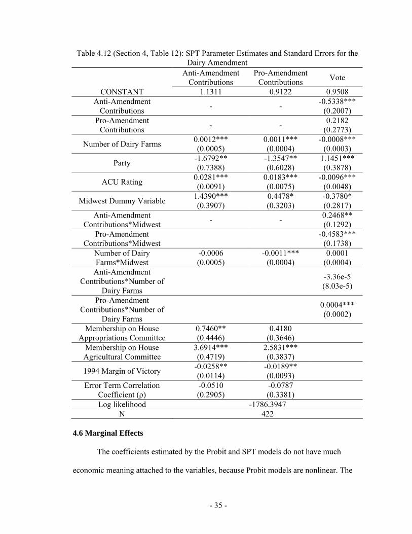
Tables 4.11 and 4.12 report the results of the FIML (SPT) model. The estimates

are not substantially different from the single equation models. The signs are the same,

and the magnitudes are in the same ranges. The predictions generally hold true. The

- 34 -

estimates are similar, because the correlation between the error terms, ρ, is small. This

implies that little additional information was gained by allowing for correlation of error

terms between the vote and contribution functions. Furthermore, because ρ is not

statistically significant from zero, we cannot reject the null hypothesis of no simultaneity

between the voting and contribution equations. Hence, single equation techniques

estimate the coefficient values consistently.

The biggest difference between the two models is evident in the dairy vote. The

coefficient estimate of the pro-contributions variable is highly significant in the single

equation model, but insignificant in the SPT model. The interaction between the number

of dairy farms and the Midwest dummy variable is also no longer significant.

Table 4.11 (Section 4, Table 11): SPT Parameter Estimates and Standard Errors for

Cotton, Peanut and Sugar Amendments Cotton Amendment Peanut Amendment Sugar Amendment Contributions Vote Contributions Vote Contributions Vote

CONSTANT -0.6951 -0.0395 -4.7575 -0.5492 3.2606 -0.8872

Contributions - 0.1913* (0.1338) - 0.4113***

(0.1179) - 0.2771*** (0.0511)

Number of Cotton, Peanut or

Sugar beet Farms

0.1709*** (0.0522)

0.5330***(0.2111)

0.5757*** (0.0955)

0.1419 (0.2387)

0.9356*** (0.2401)

6.7308** (3.5574)

Number of Sugarcane Farms - - - - 3.4764***

(1.1173) 6.7930

(5.6270)

Party -0.7081 (0.8816)

-1.276***(0.3927)

-2.8930** (1.3025)

-1.1529***(0.3858)

-1.933* (1.4264)

-1.0761***(0.4224)

ACU Rating 0.0160* (0.0111)

0.0123***(0.0048)

0.0331** (0.0159)

0.0119***(0.0047)

0.0172 (0.0175)

0.0066* (0.0051)


0.5836***(0.1598)

1.6617*** (0.5598)

1.0246***(0.1589)

1.572*** (0.6175)

0.4397*** (0.1762)


Committee

1.2205*** (0.5137) - 1.8091***

(0.7199) - 1.7400** (0.8020) -


3.6853*** (0.5175) - 6.2664***

(0.7326) - 8.4250*** (0.8894) -


(0.0198) - -0.0287* (0.0216) -

Error Term Correlation Coefficient (ρ)

-0.0950 (0.1842)

0.0758 (0.1427)

0.1257 (0.1812)

Log Likelihood -612.6126 -719.3460 -1240.3387 N 420 422 425

- 35 -

Table 4.12 (Section 4, Table 12): SPT Parameter Estimates and Standard Errors for the Dairy Amendment

Anti-Amendment Contributions

Pro-Amendment Contributions Vote

CONSTANT 1.1311 0.9122 0.9508 Anti-Amendment

Contributions - - -0.5338*** (0.2007)

Pro-Amendment Contributions - - 0.2182

(0.2773)


0.0011*** (0.0004)

-0.0008*** (0.0003)

Party -1.6792** (0.7388)

-1.3547** (0.6028)

1.1451*** (0.3878)

ACU Rating 0.0281*** (0.0091)

0.0183*** (0.0075)

-0.0096*** (0.0048)


0.4478* (0.3203)

-0.3780* (0.2817)

Anti-Amendment Contributions*Midwest - - 0.2468**

(0.1292) Pro-Amendment

Contributions*Midwest -0.4583*** (0.1738)

Number of Dairy Farms*Midwest

-0.0006 (0.0005)

-0.0011*** (0.0004)

0.0001 (0.0004)

Anti-Amendment Contributions*Number of

Dairy Farms -3.36e-5

(8.03e-5)

Pro-Amendment Contributions*Number of

Dairy Farms 0.0004***

(0.0002)

Membership on House Appropriations Committee

0.7460** (0.4446)

0.4180 (0.3646)


3.6914*** (0.4719)

2.5831*** (0.3837)


-0.0189** (0.0093)


-0.0510 (0.2905)

-0.0787 (0.3381)

Log likelihood -1786.3947 N 422

4.6 Marginal Effects

The coefficients estimated by the Probit and SPT models do not have much

economic meaning attached to the variables, because Probit models are nonlinear. The

- 36 -

coefficient estimates denote the change in the Probit index from a one unit change in the

explanatory variable. Because of the S-shaped curve of the Probit function, the impact of

an additional thousand dollar contribution or farm in a district depends on where on the

distribution we are considering. For example, a congressman already receiving $50,000

in contributions is less likely to be influenced by a $1,000 contribution than a

congressman receiving only $2,000 in contributions.

One way of interpreting the results is to look at the marginal effect on the

probability of voting “yes” from an infinitesimal change in an explanatory variable

Pr( 1)

i

VOTEX

⎛ ⎞∂ =⎜ ⎟∂⎝ ⎠

at the sample means. Since the probability density function of a Probit

model is nonlinear, the average “representative” observation is used as a reference point.

One way of calculating the marginal effect of a Probit model is by multiplying the

estimated coefficient of the relevant explanatory variable by the height of the normal

density function at the Probit index.16 Table 4.13 reports the marginal effects of each

explanatory variable in the voting equation. The single equation model predicts a 2.59

percentage point increase in the probability of voting to keep sugar price supports when

the “average” legislator receives an additional $1,000, while the SPT model predicts a

2.42 percentage point increase. Similarly, the single equation model suggests that an

additional $1,000 contribution from peanut groups increases the probability of voting for

price supports by approximately 16.9 percentage points, while the SPT model predicts a

15.9 percentage point increase.

16 The height of the normal density function is calculated as follows: 21 1exp

22z

π⎛ ⎞−⎜ ⎟⎝ ⎠

, where z is the

probit index at the sample means.

- 37 -

Table 4.13 (Section 4, Table 13): Single Equation and FIML Marginal Effects Cotton

Amendment Peanut

Amendment Sugar

Amendment Dairy

Amendment Single

Equation Probit

FIML Probit

Single Equation

Probit

FIML Probit

Single Equation

Probit

FIML Probit

Single Equation

Probit

FIML Probit

Contributions Against

Amendment 0.0450 0.0622 0.1687 0.1591 0.0259 0.0242 -0.1950 -0.1866

Contributions in Favor of Amendment

- - - - - - 0.0791 0.0833

Number of Cotton,

Peanut, Sugar beet or Dairy

Farms

0.1725 0.1733 0.0575 0.0549 0.5724 0.5879 -0.0071 -0.0017

Number of Sugarcane

Farms - - - - 0.5760 0.5879 - -

Party -0.4046 -0.3833 -0.4203 -0.4172 -0.0894 -0.0938 0.4275 0.4279 ACU Rating 0.0043 0.0040 0.0045 0.0046 0.0006 0.0006 -0.0035 -0.0037

South Dummy Variable 0.1825 0.1768 0.3579 0.3623 0.0316 0.0345 - Midwest Dummy Variable

- - - - - - -0.1516 -0.1568

4.7 Predictions of the Model

The model can be used to predict voting outcomes under different circumstances.

Table 4.7 shows that if contributions had been cut in half, the outcomes of the cotton,

peanut and sugar amendments would have been reversed and farming interests would

have lost. The model predicts that without the influence of contributions the dairy

amendment would have passed by an even greater amount. This is not surprising, because

the anti-marketing orders group contributed more money and the amendment would have

benefited more dairy farmers as they more further from Wisconsin.

However, the predictions in Table 4.14 should be considered from the proper

framework. If it were possible to reduce or eliminate PAC contributions, interest groups

would switch to different methods of exerting pressure on congressmen, such as hiring

- 38 -

lobbyists or launching advertising campaigns. The predictions also suggests uniform

effects of spending, but some votes might have changed even without contributions.

While this thought experiment is interesting, the hypothetical results should not be used

to predict the effects of campaign finance reform.

Table 4.14 (Section 4, Table 14): Predicted Voting Outcomes Under Different

Circumstances Using SPT Model

Actual Vote

Predicted Vote

Predicted Vote with Half Contributions

Predicted Vote with No Contributions

Cotton Amendment 167-253 176-244 294-126 302-118

Peanut Amendment 209-212 242-179 257-164 273-148

Sugar Amendment 208-217 235-190 290-135 386-39

Dairy Amendment 258-164 296-126 340-82 388-34

5 Conclusion

This thesis looked at the influence of campaign contributions on legislative voting.

In choosing to examine the effect of campaign contributions on the 1996 Farm Bill, the

hope was that this case study would be a good study of the ability of special interest

groups’ collective power to influence policy. The Farm Bill has a great amount of

influence over what we eat, but few people are aware of the role that government plays in

agriculture. Indeed, this is what farming groups prefer and why they are so powerful.

Theoretically, when the benefits of collective action are large and the costs are spread

throughout entire society, special interest groups have a greater incentive to organize and

the general public is less likely to protest.

The theory in Section 1 laid out the theory behind contributions and roll call

behavior. Models of legislative voting assume that politicians act rationally. The simple

- 39 -

Downsian model predicts convergence towards the median voter’s preferences if the only

determinant of attracting votes is the politician’s platform. However, when assumptions

of the model are broken, politicians may not necessarily act in the interests of society as a

whole. They consider tradeoffs between satisfying constituents’ preferences and

attracting campaign contributions. Politicians accept contributions up to the point where

the marginal benefit of an additional donation is equal to the marginal cost of moving

away from constituents’ preferred platform. The model also shows that contributors

donate in order to influence voting and affect the composition of the legislature. They

contribute up to the point where the marginal benefit of a donation is equal to the

marginal cost of a donation.

The empirical analysis performed for this thesis tested whether or not campaign

contributions influence politicians’ voting. While the answer would seem obvious to

nearly everyone, the empirical evidence in the academic literature has been mixed. Much

of the literature has attempted to address the possible simultaneity between contributions

and voting. This thesis uses Chappell’s empirical model to account for the possibility of

simultaneity. The results show that contributions, constituent interests, ideology and

political party are all determinants of a politician’s voting function. The more cynical

among us can take some comfort in knowing that politicians consider voters’ interests.

The marginal effect of a change in contributions from cotton groups on voting in

favor of cotton subsidies is 0.0622 for the average representative legislator. Similarly the

marginal effects of changes in peanut contributions and sugar contributions on voting for

price supports are 0.1591 and 0.0242, respectively. The marginal effect of a change in

- 40 -

contributions from an anti-marketing orders dairy group is -0.1137, while the marginal

effect of a change in donation from a pro-marketing dairy group is 0.2575.

The empirical model used in this thesis cannot possibly capture the complex

nature of legislation crafting and political maneuvering. Special interest groups exert their

influence in ways besides campaign contributions. Many groups hire lobbyists to build

relationships with legislators. Interest groups can influence legislation even before it is

sent to the floor for a vote. When proposals of a bill are being drafted in committee,

special interest groups very often have a say in what is included and excluded from the

bill. Exceptions and loopholes sometimes defeat the intent of the bill. Compared to such

shrouded methods, campaign contributions are transparent and above-board. If possible,

future research should attempt to study the other kinds of behavior that special interest

groups exhibit. However, given the nature of these groups, finding ideal data could be a

daunting task.

Appendix A: List of Special Interest Groups by Amendment

Cotton Groups American Cotton Shippers Association Arizona Cotton Growers Association PAC California Cotton Growers Association PAC Cotton Warehouse Government Relations Committee Committee for the Advancement of Southeastern Cotton (CASC) / Southern Cottongrowers Inc. / Southeastern Cotton Ginners Assocation J.G. Boswell Company Employees’ PAC National Cotton Council Committee for the Advancement of Cotton New York Cotton Exchange PAC Plains Cotton Cooperative Association Employees PAC Peanut Groups Alabama Peanut Producers Association American Peanut Shellers PAC Georgia Peanut Producers Association PAC Nutpac Peanut and Tree Nut Processors Association PAC Southwest Peanut PAC

- 41 -

Virginia-Carolina’s Peanut Membership Organization PAC Western Peanut Growers PAC Sugar Groups Amalgamated Sugar Company PAC American Crystal Sugar American Sugar Cane League American Sugarbeet Growers Assocation Flo-Sun Inc. Florida Sugar Cane Leagut Great Lakes Sugar Beet Growers Assocation Hawaiian Sugar Planters Association Imperial Holly Corporation Refined Sugars Inc. Rio Grande Valley Sugar Growers Savannah Foods & Industries Southern Minnesota Beet Sugar Cooperative Sugar Cane Growers Cooperative of Florida Texas Sugar Beet Growers Association United States Beet Sugar Association United States Sugar Corp United States Sugar Corporation Anti-Marketing Orders Dairy Groups Agri-Mark Arizona Dairymen Blue Bill Creameries California Cooperative Creamery Dairylea Cooperative Dairyman’s Cooperative Creamery Association Danish Creamery Association Federal PAC Royal Crest Dairy Michigan Milk PAC Mid-America Dairymen Robinson Dairy Western United Dairymen’s Association Federal PAC Pro-Marketing Orders Dairy Groups Associated Milk Producers Darigold PAC (North Pacific Dairymen’s Cooperative Trust) International Dairy Foods Assocation (IDFA) / Milk Industry Foundation (MIF) / National Cheese Institute (NCI) and the Ice Cream Assocation (IICA) Land O’Lake Leprino Milk Marketing Inc. United Dairy Farmers

- 42 -

Appendix B: SPT Regressions with Alternative Measures of Agricultural Importance

Table B.1 (Appendix B, Table 1): SPT Parameter Estimates and Standard Errors for Cotton, Peanut and Sugar Amendments with Harvest Variable

Cotton Amendment Peanut Amendment Sugar Amendment Contributions Vote Contributions Vote Contributions Vote

CONSTANT -0.4678 -0.0450 -4.6377 -0.5502 3.2620 -0.8978

Contributions - 0.1833* (0.1372) - 0.4136***

(0.1178) - 0.2792*** (0.0513)

Thousands of Acres of Cotton, Peanut or

Sugar beet Harvested

0.0037*** (0.0010)

0.0177***(0.0076)

0.0569*** (0.0091)

0.0218 (0.0264)

0.0483*** (0.0123)

0.0997 (0.0960)

Thousands of Acres of Sugarcane Harvested - - - - 0.0795***

(0.0151) 0.0314** (0.0152)

Party -0.8116 (0.8634)

-1.2706***(0.3931)

-2.7245** (1.2904)

-1.1431***(0.3857)

-2.2667** (1.3893)

-1.1901***(0.4287)

ACU Rating 0.0173* (0.0109)

0.0123***(0.0048)

0.0314** (0.0158)

0.0118***(0.0047)

0.0228* (0.0170)

0.0084** (0.0052)


0.5619***(0.1611)

1.6837*** (0.5524)

1.0172***(0.1583)

1.2331** (0.6008)

0.3805** (0.1736)


Committee

1.2449*** (0.5070) - 1.8584***

(0.7120) - 1.8128*** (0.7792) -


3.5491*** (0.5119) - 6.2090***

(0.7255) - 8.2341*** (0.8615) -


(0.0196) - -0.0292* (0.0210) -


-0.0829 (0.1881)

0.0683 (0.1430)

0.1226 (0.1802)

Log Likelihood -609.6039 -718.1752 -1240.3387 N 420 422 425

Table B.2 (Appendix B, Table 2): SPT Parameter Estimates and Standard Errors for

Cotton, Peanut and Sugar Amendments with Production Variable Cotton Amendment Peanut Amendment Sugar Amendment Contributions Vote Contributions Vote Contributions Vote

CONSTANT -0.3536 -0.0426 -4.6105 -0.5503 3.2538 -0.9007

Contributions - 0.1686 (0.1445) - 0.4127***

(0.1178) - 0.2801*** (0.0514)

Thousands of Pounds of Cotton, Peanut or Sugar beet Produced

0.0048*** (0.0009)

0.0147** (0.0064)

2.35e-05*** (1.30e-06)

8.43e-06 (1.1e-05)

0.0026*** (0.0006)

0.0036 (0.0033)

Thousands of Acres of Sugarcane Produced - - - - 0.0795***

(0.0151) 0.0009** (0.0005)

Party -0.7562 (0.8158)

-1.2916***(0.3911)

-2.8710** (1.2974)

-1.1508***(0.3850)

-2.2911** (1.3868)

-1.1754***(0.4279)

ACU Rating 0.0175** (0.0103)

0.0125***(0.0048)

0.0335** (0.0159)

0.0118***(0.0047)

0.0228* (0.0170)

0.0083* (0.0052)

- 43 -


0.5916***(0.1608)

1.7277*** (0.5551)

1.0210***(0.1582)

1.2453** (0.6005)

0.3881** (0.1738)


Committee

1.1787*** (0.4804) - 1.8470***

(0.7168) - 1.8108*** (0.7786) -


3.1578*** (0.4917) - 6.2429***

(0.7304) - 8.1915*** (0.8621) -


(0.0197) - -0.0290* (0.0209) -


-0.0556 (0.1938)

0.0720 (0.1430)

0.1192 (0.1783)

Log Likelihood -602.8300 -719.0659 -1234.7013 N 420 422 425

Appendix C: Regressions with Interaction Terms

Table C.1 (Appendix C, Table 1): SPT Parameter Estimates and Standard Errors for

Cotton, Peanut and Sugar Amendments with Interaction Terms COTTON PEANUT SUGAR COTTON CONTRIB PEANUT CONTRIB SUGAR CONTRIB

CONSTANT -0.7575 -0.2087 -4.7423 -0.6931 3.1867 -0.9396

Contributions 1.5977***(0.5400) 0.8724***

(0.2313) - 0.2945***(0.0662)

Number of Cotton, Peanut or Sugar Beet Farms

0.1657***(0.0516)

0.4488** (0.2393)

0.5718***(0.0951)

0.1778 (0.2689)

0.9329*** (0.2399)

7.655** (3.8936)

Number of Sugarcane Farms - 3.4760*** (1.1168)

-4.3555 (16.3240)

Party -0.7142 (0.8812)

-0.9575** (0.4237)

-2.8359**(1.2956)

-1.3195*** (0.4282)

-1.9247* (0.4260)

-1.3815**(0.6030)

ACU Rating 0.0160* (0.0111)

0.0099** (0.0051)

0.0322** (0.0158)

0.0156*** (0.0052)

0.0171 (0.0175)

0.0063** (0.0073)

South Dummy Variable 1.1583***(0.4034)

0.6821***(0.1697)

1.6407***(0.5576)

0.9724*** (0.1809)

1.5588*** (0.6168)

0.9100***(0.2650)

Contributions*Number of Cotton, Peanut or Sugar Beet

Farms - 0.0012

(0.0027) - -0.0001 (0.0008) -0.0033**

(0.0020)

Contributions*Party - -0.8900 (1.105) - 0.7730

(0.6591) 0.1299 (0.1675)

Contributions*ACU Rating - -0.0033 (0.0129) - -0.0139**

(0.0078) -0.0001 (0.0020)

Contributions*South - -0.3858** (0.2282) - 0.1115

(0.2252) -

0.1620***(0.0647)

APPROP 1.2376***(0.5014)

1.201*** (0.5192)

1.8520***(0.7150)

1.8487*** (0.7211)

1.7374** (0.8031)

AG 3.7767***(0.4971)

3.6459***(0.5083)

6.3668***(0.7259)

6.3708*** (0.7246)

8.4549*** (0.8873)

MARGIN -0.0451***(0.0152)

-0.0468***(0.0159)

0.0062 (0.0197)

0.0062 (0.0199)

-0.0275 (0.0216)

Correlation Coefficient (ρ) -0.3425 -0.0437 0.0763 Log likelihood -604.9976 -715.9377 -1234.4865

N 420 422 425

- 44 -

Table C.2 (Appendix C, Table 2): SPT Parameter Estimates and Standard Errors for the Dairy Amendment with Interaction Terms

Contributions Against Amendment

Contributions For Amendment Vote

CONSTANT 1.164 0.9036 1.1876 Contributions Against

Amendment - - -1.0312*** (0.2735)

Contributions for Amendment - - 0.4790* (0.3061)


0.0679*** (0.0212)

-0.0461*** (0.0182)

Party -1.6940** (0.7403)

-1.3686** (0.6021)

0.6574* (0.4936)

ACU Rating 0.0284*** (0.0091)

0.0184*** (0.0074)

-0.0076* (0.0059)


0.4581* (0.3181)

-0.3704* (0.2858)

Contributions Against Amendment* Number of Dairy

Farms - - -0.0029

(0.0060)

Contributions for Amendment* Number of Dairy Farms - - 0.0334***

(0.0115) Contributions Against

Amendment*Party - - 0.5542* (0.3821)

Contributions for Amendment* Party - - -0.1761

(0.4149) Contributions Against

Amendment*ACU Rating - - 0.0011 (0.0044)

Contributions for Amendment* ACU Rating - - -0.0031

(0.0047) Contributions Against Amendment*Midwest - - 0.2276**

(0.1274) Contributions for Amendment*

Midwest - -0.4920*** (0.2069)

Number of Dairy Farms* Midwest

-0.0282 (0.0292)

-0.0677*** (0.0235)

0.0011 (0.0273)

Membership on Appropriations Committee

3.7354** (0.4468)

0.4294 (0.3646) -

Membership on Agricultural Committee

3.7354*** (0.4712)

2.5935*** (0.3814) -


-0.0188** (0.0093) -

Correlation Coefficient (ρ) -0.0543 (0.2976)

-0.0240 (0.3292) -

Log likelihood -1775.8908 N 422

- 45 -

Bibliography

Abler, D. G. 1991. Campaign contributions and house voting on sugar and dairy legislation. American Journal of Agricultural Economics 73, no. 1: 11-17.

Ansolabehere, Stephen, John M. de Figueiredo, and James M. Snyder, Jr. 2003. Why is there so little money in u.S. Politics? Journal of Economic Perspectives 17, no. 1: 105-130.

Baldwin, R. E. and C. S. Magee. 2000. Is trade policy for sale? Congressional voting on recent trade bills. Public Choice 105, no. 1-2: 79-101.

Becker, Gary S. 1983. A theory of competition among pressure groups for political influence. The Quarterly Journal of Economics 98, no. 3: 371-400.

Black, Duncan. 1948. On the rationale of group decision-making. Journal of Political Economy, no. 56: 23-54.

Bronars, Stephen G. and John R. Lott, Jr. 1997. Do campaign donations alter how a politician votes? Or, do donors support candidates who value the same things that they do? Journal of Law and Economics 40, no. 2: 317-350.

Brooks, Jonathan C., A. Colin Cameron, and Colin A. Carter. 1998. Political action committee contributions and u.S. Congressional voting on sugar legislation. American Journal of Agricultural Economics 80, no. 3: 441-454.

Chappell, Henry W., Jr. 1981. Campaign contributions and voting on the cargo preference bill: A comparison of simultaneous models. Public Choice 36, no. 2: 301-312.

________. 1982. Campaign contributions and congressional voting: A simultaneous probit-tobit model. The Review of Economics and Statistics 64, no. 1: 77-83.

Clawson, Dan, Alan Neustadtl, and Denise Scott. 1992. Money talks: Corporate pacs and political influence. New York: Basic Books.

Downs, Anthony. 1957. An economic theory of democracy. New York: Harper Collins. Ellison, S. F. and W. P. Mullin. 1995. Economics and politics - the case of sugar tariff

reform. Journal of Law & Economics 38, no. 2: 335-366. Gardner, Bruce L. 2002. American agriculture in the twentienth century: How it

flourished and what it cost. Cambridge, Massachusetts: Havard University Press. Gawande, Kishore and Bernard Hoekman. 2006. Lobbying and agricultural trade policy

in the united states. International Organization 60, no. 3: 527-561. Grossman, G. M. and E. Helpman. 1994. Protection for sale. American Economic Review

84, no. 4: 833-850. Imhoff, Daniel. 2007. Foodfight: The citizen's guide to a food and farm bill. Healdsburg,

California: Watershed Media. Kau, James B., Donald Keenan, and Paul H. Rubin. 1982. A general equilibrium model

of congressional voting. The Quarterly Journal of Economics 97, no. 2: 271-293. Levitt, Steven D. 1995. Policy watch: Congressional campaign finance reform. Journal of

Economic Perspectives 9, no. 1: 183-193. Magee, C. 2002. Do political action committees give money to candidates for electoral or

influence motives? Public Choice 112, no. 3-4: 373-399. Mueller, Dennis C. 2003. Public choice iii: Cambridge; New York and Melbourne:

Cambridge University Press.

- 46 -

Nicholson, Walter. 2005. Microeconomic theory: Basic principles and extensions. Mason, Ohio: Thomson/South-Western.

Olson, Mancur. 1965. The logic of collective action: Public goods and the theory of groups. Cambridge: Harvard University Press.

Peltzman, S. 1984. Constituent interest and congressional voting. Journal of Law & Economics 27, no. 1: 181-210.

Roscoe, D. D. and S. Jenkins. 2005. A meta-analysis of campaign contributions' impact on roll call voting. Social Science Quarterly 86, no. 1: 52-68.

Stratmann, T. 2005. Some talk: Money in politics. A (partial) review of the literature. Public Choice 124, no. 1-2: 135-156.

Stratmann, Thomas. 1991. What do campaign contributions buy? Deciphering causal effects of money and votes. Southern Economic Journal 57, no. 3: 606-620.

________. 1992. Are contributions rational? Untangling strategies of political action committees. Journal of Political Economy 100, no. 3: 647-664.

________. 2002. Can special interests buy congressional votes? Evidence from financial services legislation. Journal of Law and Economics 45, no. 2: 345-373.

U.S. General Accounting Office. 2000. “Sugar program.” GAO/RCED-00-126. June. Van Doren, T. D., D. L. Hoag, and T. G. Field. 1999. Political and economic factors

affecting agricultural pac contribution strategies. American Journal of Agricultural Economics 81, no. 2: 397-407.

Wanlass, William L. 1920. “The United States Department of Agriculture.” Johns Hopkins University Studies in Historical and Political Science no. 38: 12-31.

Welch, W. P. 1981. Money and votes: A simultaneous equation model. Public Choice 36, no. 2: 209-234.

________. 1982. Campaign contributions and legislative voting: Milk money and dairy price supports. The Western Political Quarterly 35, no. 4: 478-495.

Wilson, James Q. 1989. Bureaucracy: What government agencies do and why they do it. New York: Basic Books.

Wolaver, Amy M. and Christopher S. Magee. 2006. The effects of political action committee contributions on medical liability legislation. B.E. Journals in Economic Analysis and Policy: Topics in Economic Analysis and Policy 6, no. 1: 1-21.

The Influence of Campaign Contributions on Legislative ... · The Influence of Campaign...

Documents

Transcript of The Influence of Campaign Contributions on Legislative ... · The Influence of Campaign...