The Impacts of Ultra High Voltage AC line characteristics ...1039138/FULLTEXT01.pdf · The Impacts...
58
IN DEGREE PROJECT ELECTRICAL ENGINEERING, SECOND CYCLE, 30 CREDITS , STOCKHOLM SWEDEN 2016 The Impacts of Ultra High Voltage AC line characteristics on line distance protection KARTHI TAMILSELVAN KTH ROYAL INSTITUTE OF TECHNOLOGY SCHOOL OF ELECTRICAL ENGINEERING
Transcript of The Impacts of Ultra High Voltage AC line characteristics ...1039138/FULLTEXT01.pdf · The Impacts...
IN DEGREE PROJECT ELECTRICAL ENGINEERING,SECOND CYCLE, 30 CREDITS
, STOCKHOLM SWEDEN 2016
The Impacts of Ultra High Voltage AC line characteristics on line distance protection
KARTHI TAMILSELVAN
KTH ROYAL INSTITUTE OF TECHNOLOGYSCHOOL OF ELECTRICAL ENGINEERING
i
The Impacts of Ultra High Voltage
AC line characteristics on traditional
line distance protection
Master thesis
By
Karthi Tamilselvan
Supervisors
Jianping Wang, ABB Corporate Research Center
Nathaniel Taylor, KTH School of Electrical Engineering
Examiner
Hans Edin, KTH School of Electrical Engineering
Royal Institute of Technology
Department of Electrical Engineering
Electromagnetic Engineering
Stockholm 2016
ii
Abstract
With the growing load demand, Ultra high Voltage (UHV) transmission lines are utilized in
many countries around the world for bulk power transmission from remote locations over long
distance. UHV transmission lines have typical features and it poses a challenge to the power
system design with respect to protection, insulation and reactive power compensation, etc.
Protection is a key issue in UHV transmission since a relay failure can interrupt and damage
the power system. There are distance and differential protection schemes in the transmission
line which account for security of the power system.
This thesis report is based on analysis carried out to find out the typical features associated
with the UHV transmission systems. Also the impacts of the UHV transmission line
characteristics on line distance protection scheme are observed. The traditional distance relays
based on the lumped line parameters are not suited for the UHV transmission lines of very long
distances. In this case a simulation is carried out for a 765 kV transmission system modeled in
PSCAD. In such a case the non-linearity is even more prominent and the relay is less
dependable. In line with the simulation and the analysis for the challenges in UHV transmission
system, it is observed that the fault impedance of the line is non-linear and this non-linearity
causes the failure of relay operation for a fault location at the boundary of the zone of
protection.
The fault simulation was carried out in PSCAD and the quadrilateral distance relay
characteristics were plotted using MATLAB. From the simulation and results, it is finally
concluded that traditional distance protection relays with lumped parameter line modeling is
not suitable for UHV transmission liens due to non-linearity in fault impedance and it leads to
relay failure.
Keywords: UHV transmission line, line distance protection, non-linearity of fault impedance.
iii
Sammanfattning
Ultra high voltage (UHV) transmissionsledningar används i många länder till följd av ett
växande behov av överföra hög effekt från avlägset belägna produktionsanläggningar till
konsumenter. UHV-transmissionsledningar har speciella egenskaper som innebär utmaningar
vid designandet av kraftsystem. Några utmaningar är systemskydd, isolation, och reaktiv
effektkompensering. Systemskydd är en viktig aspekt för UHV-transmission eftersom haveri
av reläskydd kan orsaka driftstopp och även skada ett kraftsystem. Det finns distans- och
differentialskydd i transmissionsledningar som utgör skydd för kraftsystemet.
Denna avhandling är baserad på analyser som har utförts för att åskådliggöra de typiska
egenskaperna som är sammankopplade med UHV-transmissionssystem. Även inverkan på
distansskydd orsakad av karaktäristiken av UHV-transmissionsledningar utvärderas. De
traditionella distansreläskydden som baseras på de sammanslagna ledningsparametrarna är inte
lämpade för UHV-transmissionsledningar som stäcker sig över långa avstånd. I detta fall har
en simulering utförts i PSCAD för ett transmissionssystem med spänningen 765 kV. I ett sådant
fall är karaktäristiken ännu mer olinjär och reläskydden ännu mindre pålitliga. Det observeras
att felimpedansen för ledningen är olinjär och till följd av detta orsakas problem med
reläskydden då ett fel uppkommer vid utkanten av den skyddade zonen. Denna observation
överensstämmer med simuleringarna och de förväntade utmaningarna kopplade till UHV.
Simuleringar av felfall utfördes i PSCAD och karaktäristiken av reläskydden plottades med
hjälp av MATLAB. Från resultat presenteras i rapporten, konkluderas det att konventionella
distansskyddsreläer med modellering av sammanslagna ledningsparametrar inte är lämpliga
för UHV-transmissionsledningar på grund av att den olinjära felimpedansen leder till att
reläskydden havererar.
Nyckelord: UHV transmissionsledningar, distans- skydd, olinjära felimpedansen.

iv
Acknowledgement
This thesis work is a fulfilment of the Master degree programme in Electric Power Engineering
at Kungliga Tekniska Högskolan (KTH Royal Institute of Technology) carried out at ABB
Corporate Research Centre’s (SECRC) Power system development division in Västerås,
Sweden.
I would like to thank everyone who had supported me and helped me to achieve this feat. I
would like to thank Robert Saers for providing me an opportunity to do my thesis at ABB
SECRC and his support throughout the thesis work.
I am very grateful to Professor Hans Edin for the approval to work on the project as my master’s
degree thesis and acceptance to be my examiner at KTH and for his positive interactions.
I would like to express my gratitude to my supervisor Jianping Wang at ABB Corporate
Research for his constant encouragement and patience during the entire work and for
introducing me into the research world.
I am very thankful to my supervisor Nathaniel Taylor at KTH for his suggestions in the project
and for his kind patience in answering our queries for the entire duration of the thesis work.
I would also like to thank Monika Koerfer at ABB for her kind support and help in arranging
everything that is needed at SECRC.
Further, I would take the opportunity to thank all my friends at ABB and KTH who had been
with me in all tough times and helping me to get through the thesis work.
Finally, I owe my huge respect and thanks to my family for their love, support and kindness to
help me get over obstacles and provide support for my entire duration of studies.
v
CONTENTS 1 Introduction ........................................................................................................................ 1
1.1 Problem Definition ...................................................................................................... 2
1.2 Objectives of the Thesis .............................................................................................. 2
1.3 Method ........................................................................................................................ 2
1.4 Outline of the Thesis ................................................................................................... 2
2 History and Development of UHV Transmission Technology .......................................... 4
2.1 Development of Transmission Grid and Voltage Upgrade ......................................... 4
2.2 Development of UHV Transmission System Technology .......................................... 5
2.3 Advantages of UHV AC Lines.................................................................................... 6
2.4 Existing and upcoming UHV Transmission Lines Worldwide ................................... 7
3 Need for line model ............................................................................................................ 9
3.1 Choice of the model .................................................................................................... 9
3.1.1 Frequency dependent line model ......................................................................... 9
3.2 Line model in PSCAD............................................................................................... 11
3.2.1 Type of conductors ............................................................................................ 11
3.2.2 Surge Impedance loading ................................................................................... 13
3.2.3 Overhead transmission line parameter ............................................................... 14
4 Analysis of typical features of UHV transmission systems ............................................. 16
4.1 Model of the Test system .......................................................................................... 16
4.2 DC component time constant .................................................................................... 16
4.3 Phase difference ........................................................................................................ 17
4.4 Shunt reactor compensation ...................................................................................... 18
4.5 Line energization ....................................................................................................... 20
4.6 Capacitance line charging current ............................................................................. 21
4.7 Line model and non-linearity in impedance .............................................................. 23
5 Fault impedance transients ............................................................................................... 28
5.1 Fault transients and its types ..................................................................................... 28
5.2 Traditional protection algorithm ............................................................................... 29
6 Closure .............................................................................................................................. 46
6.1 Conclusions ............................................................................................................... 46
6.2 Future work ............................................................................................................... 47
vi
LIST OF FIGURES Figure 3.1: Distributed Line parameter model ...................................................................................... 10
Figure 3.2: line geometry ...................................................................................................................... 12
Figure 3.3: Sending and receiving end voltage relationship Under SIL ............................................... 14
Figure 4.1: UHV transmission line model with two sources for simulation ......................................... 16
Figure 4.2: Comparison of DC decay time for 765kV and 230kV transmission line ........................... 17
Figure 4.3: Phase difference between sending and receiving end voltages at SIL ............................... 18
Figure 4.4: RMS value of voltage at the sending and receiving ends without shunt reactor
compensation ........................................................................................................................................ 19
Figure 4.5: RMS value of voltage at the sending and receiving ends with shunt reactor compensation
.............................................................................................................................................................. 20
Figure 4.6: Overvoltage during line energization ................................................................................. 21
Figure 4.7: Self and mutual capacitances of OHL ................................................................................ 22
Figure 4.8: Line charging current for 765kV ........................................................................................ 22
Figure 4.9: Fault impedance in R-X plane for 3 phase faults ............................................................... 24
Figure 4.10: Line impedance for a 3 phase fault ................................................................................... 25
Figure 4.11: Fault impedance in R-X plane for LL faults ..................................................................... 25
Figure 4.12: Fault impedance for LL phase fault as a variation of fault locations ............................... 26
Figure 4.13: Fault impedance in R-X plane for LG faults .................................................................... 27
Figure 4.14: Fault impedance for single phase as a variation of fault locations ................................... 27
Figure 5.1: Impedance relay with Quadrilateral characteristics in both forward and reverse directions
.............................................................................................................................................................. 30
Figure 5.2: Phase on a transmission line ............................................................................................... 31
Figure 5.3: Simple representation of a Phase fault between a and b phases ......................................... 31
Figure 5.4: Quadrilateral relay characteristics for phase faults ............................................................. 32
Figure 5.5: Quadrilateral relay with a LLL fault on Phase A at 100 km of the transmission line ........ 33
Figure 5.6: Quadrilateral relay with a LLL fault on Phase A at 200 km of the transmission line ........ 33
Figure 5.7: Quadrilateral relay with a LLL fault on Phase A at 300 km of the transmission line ........ 34
Figure 5.8: Quadrilateral relay with a LLL fault on Phase A at 380 km of the transmission line ........ 35
Figure 5.9: Quadrilateral relay with a LLL fault on Phase A at 400 km of the transmission line ........ 35
Figure 5.10: Quadrilateral relay with a LLL fault on Phase A at 420 km of the transmission line ...... 36
Figure 5.11: Single line to ground fault on a transmission line ............................................................ 37
Figure 5.12: simple representation of the LG fault in phase ‘a’ ........................................................... 37
Figure 5.13: Quadrilateral relay setting for SLG fault .......................................................................... 38
Figure 5.14: Quadrilateral relay with a LG fault on Phase A at 100 km of the transmission line ........ 39
Figure 5.15: Quadrilateral relay with a LG fault on Phase A at 200 km of the transmission line ........ 40
Figure 5.16: Quadrilateral relay with a LG fault on Phase A at 300 km of the transmission line ........ 40
Figure 5.17: Quadrilateral relay with a LG fault on Phase A at 380 km of the transmission line ........ 41
Figure 5.18: Quadrilateral relay with a LG fault on Phase A at 400 km of the transmission line ........ 41
Figure 5.19: Quadrilateral relay with a LG fault on Phase A at 420 km of the transmission line ........ 42
Figure 5.20: LG fault at 400 km with a single source and a load at remote end ................................... 43
Figure 5.21: Quadrilateral relay with a LL fault on Phase A and Phase B at 300 km of the
transmission line ................................................................................................................................... 44
Figure 5.22: Quadrilateral relay with a LL fault on Phase A and Phase B at 400 km of the
transmission line ................................................................................................................................... 44
Figure 5.23: Quadrilateral relay with a LLG fault on Phase A and Phase B at 300 km of the
transmission line ................................................................................................................................... 45
Figure 5.24: Quadrilateral relay with a LLG fault on Phase A and Phase B at 400 km of the
transmission line ................................................................................................................................... 45
vii
LIST OF TABLES Table 2.1: Some important events on the development of transmission line voltage. ............................ 4
Table 2.2: Information of some existing UHV lines around the world [19]–[28]. ................................. 7
Table 3.1: Conductor parameters used for UHV line model ................................................................ 13
Table 3.2: Typical overhead transmission line parameter [36] ............................................................. 14
Table 3.3: Line parameters for the simulated Line model in PSCAD .................................................. 15
Table 5.1: Probability of occurrence of fault ........................................................................................ 29
1
Chapter 1
Background and Outline
1 INTRODUCTION
Modern life is highly dependent on the use of electricity. Electric power systems are
responsible to ensure the reliable and secured supply of electricity. No matter how well
designed and maintained the system is, there is always risk of faults and failures. These faults
can lead to severe damage or even system failure. Thus a protection system is required with a
focus on the corrective steps after fault occurrence. The protection system plays a significant
role to detect the faults in the system and isolate the faulted parts.
An electric power system is typically differentiated into three parts generation, transmission
and distribution. Most of the time the generation part is located in remote places and the load
density is high in the industrial and residential areas. Transmission lines or the transmission
grid transfer the generated electricity from the generation side to the load side. In case of any
fault occurrence it is very important to isolate that section of the grid to ensure fast power
restoration and continuous flow of electricity to the end user. Thus, study of transmission line
protection has been always an essential part from the early edge of electricity.
The power system has been evolving to meet the increasing demand of electricity. It has
evolved from isolated generators feeding their own loads to a huge interconnected system
covering the whole country. The voltage level and the power handling capability have been
increased due to the increasing demands. Side by side, the protection requirements have been
changed based on the evolvement of the transmission system. As a result the protection system
advanced through an era of electromechanical relays and/over, static relays to the era of
numerical protection with the advancement of available technology and system requirements
[1] .
The necessity of upgrading to the Ultra High Voltage (UHV) level comes from the requirement
of increasing the capability of transmitting more power but reducing the transmission losses at
the same time. It also helps to connect different energy sources from long distance and thus
improve the system security. Recently, engineers have become focused more on environment
friendly solutions. Increase in renewable energy sources is a demand of time for a sustainable
world. But most of the renewable energy sources are situated at remote places and the
geographical location depends on the availability of the natural resource. This requires the
interconnection between sources and loads. UHV lines can play an important role to transfer
the renewable energy from one side to another side within a long distance. The motivation
behind establishing UHV lines can lie behind some other beneficial aspects subjected to the
country’s perspective. However, voltage upgrading requires the upgrading of the ancillary parts
such as the substation technology[2],[3], insulation technology[4], the transmission tower
configuration etc.. A study on the impact of UHV transmission line on the traditional protection
schemes is equally important to ensure a reliable and secured power system.
2
1.1 PROBLEM DEFINITION
Ultra-high voltage lines have a low resistance value per unit length which results in low energy
loss hence, beneficiary from economic perspective. In order to meet the low inductance and
less corona loss, multiple conductors are bundled in UHV transmission lines [5]. This leads to
a higher distributed capacitance value. The impact of this distributed capacitance is not
significant if the line length is not long or the voltage level is not very high. However, for UHV
transmission lines with a long line length the effect of this distributed capacitance is significant
for the traditional line protection scheme. The long lines result in smaller equivalent capacitive
reactance which leads to larger capacitive charging current. However, the traditional protection
algorithms and analysis are still based on the classical lumped parameters, which may lead to
big error or even problems for the protections of UHV transmission lines. As a result, a study
should be done on how significant the impact is and how to overcome them in order to maintain
the reliability, sensitivity and security of the system.
1.2 OBJECTIVES OF THE THESIS
The thesis is focused on the impacts of UHV AC transmission lines on traditional protective
relays. The objective of the thesis can be described as follows,
Market survey on the existing UHV AC transmission lines and its applications
Modelling of UHV AC transmission line in PSCAD and validation with practical data.
Transient fault analysis for UHV AC transmission line and investigation on the special
fault phenomena.
Impacts of UHV AC line characteristics on traditional line distance protection.
1.3 METHOD
A 765 kV UHV AC transmission line is modelled in PSCAD. A frequency dependent model
is selected from PSCAD library to get the most precise results during transients. The required
input parameters for the tower configuration and conductor specification are given according
to the guidance of U.S. Department of Energy [6] and other available open source information.
Then the line parameters i.e. the sequence components of the modelled line are cross verified
with the line parameters of an existing line to make sure the validity of the modelled line.
Different types of faults along the line are introduced in order to study the line behaviour during
the transients. Later the study is done to find out the impacts on specific protection scheme and
how to overcome the challenges for that protection scheme.
1.4 OUTLINE OF THE THESIS
Chapter 1 of the thesis describes the motivation, objective and method of the thesis work.
Chapter 2 describes the development of the transmission grid, existing situation of UHV AC
transmission lines.
Chapter 3 focuses on the modelling of UHV AC transmission line and their operation.
Chapter 4 presents the UHV AC transmission line phenomena those are important for the
protection system.
3
Chapter 5 shows the challenges of existing distance protection scheme with UHV transmission
line phenomenon.
Chapter 6 provides discussions on the thesis and the conclusions as well as suggestions for the
future works.
This thesis is done in parallel with another master thesis [7] which deals with the challenges
and solutions regarding the differential protection for UHV lines. The first three chapters are
common for both of the thesis works and the study is done together. Thus these chapters are
common in both of the thesis reports. However, the rest of the works in each thesis are done
individually focusing on either the distance protection or differential protection scheme on
UHV transmission lines.
In this thesis report, the focus is mainly on the line distance protection scheme for UHV AC
transmission line.
4
Chapter 2
Market Survey
2 HISTORY AND DEVELOPMENT OF UHV TRANSMISSION
TECHNOLOGY
2.1 DEVELOPMENT OF TRANSMISSION GRID AND VOLTAGE UPGRADE
Electricity is one of the major contributors to the development of human civilization. It has
become the part and parcel of modern life. A very complex system consisting of generation,
transmission and distribution is being operated continuously to supply the electricity to the
consumers.
The first commercial AC transmission grid was built by Westinghouse and started operation in
1896 [8]. It was a 40 km long, three phase AC transmission line from Niagara Falls generating
station to Buffalo. Although DC transmission system was prominent at that time, it was
dominated by AC technology due to its lower transmission loss. The successful implementation
of transformers in AC transmission technology made it possible to increase the transmission
voltage level which allowed transferring the same amount of power but with lower current i.e.
lower loss.
Since then the development of the transmission grid has been designed depending on the world
war, single unit generation capacity was not more than 200 MW and the dominant transmission
voltage was up to 220 kV [9]. Typically, the grid size was small and isolated, thus long distance
transmission line was not a required. After the second world war, there was rapid increase in
demand of electricity due to the industrialization. The generating capacity also increased and
the transmission line voltage went up in order to transmit large amount of power in long
distance [10].
Another important phenomenon is the integration of the grid. The grid interconnection took
place to balance loads and improve load factors between interconnected central stations.
Interconnection became increasingly desirable in order to ensure the availability and reliability
that cross border interconnection started to take place in later of the twentieth century. Thus
transmission lines interconnecting two countries or two regions required to transmit huge
amount of power in very long distances with maximum efficiency. As a result, transmission
voltages also climbed up in steps from high voltage to ultra-high voltage. Some significant
landmarks in the history of AC transmission grid are depicted in Table 2.1[9].
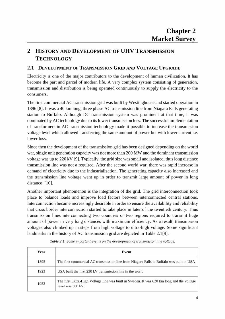
Table 2.1: Some important events on the development of transmission line voltage.
Year Event
1895 The first commercial AC transmission line from Niagara Falls to Buffalo was built in USA
1923 USA built the first 230 kV transmission line in the world
1952 The first Extra-High Voltage line was built in Sweden. It was 620 km long and the voltage
level was 380 kV.
5
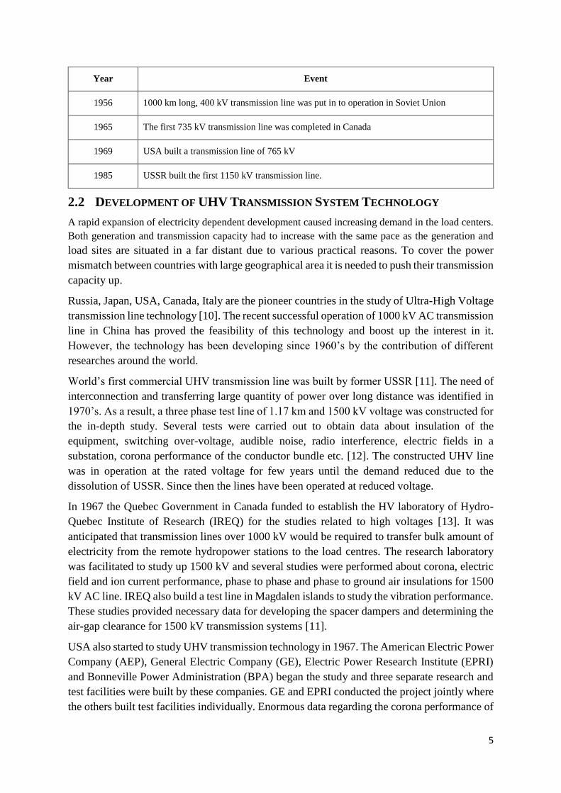
Year Event
1956 1000 km long, 400 kV transmission line was put in to operation in Soviet Union
1965 The first 735 kV transmission line was completed in Canada
1969 USA built a transmission line of 765 kV
1985 USSR built the first 1150 kV transmission line.
2.2 DEVELOPMENT OF UHV TRANSMISSION SYSTEM TECHNOLOGY
A rapid expansion of electricity dependent development caused increasing demand in the load centers.
Both generation and transmission capacity had to increase with the same pace as the generation and
load sites are situated in a far distant due to various practical reasons. To cover the power
mismatch between countries with large geographical area it is needed to push their transmission
capacity up.
Russia, Japan, USA, Canada, Italy are the pioneer countries in the study of Ultra-High Voltage
transmission line technology [10]. The recent successful operation of 1000 kV AC transmission
line in China has proved the feasibility of this technology and boost up the interest in it.
However, the technology has been developing since 1960’s by the contribution of different
researches around the world.
World’s first commercial UHV transmission line was built by former USSR [11]. The need of
interconnection and transferring large quantity of power over long distance was identified in
1970’s. As a result, a three phase test line of 1.17 km and 1500 kV voltage was constructed for
the in-depth study. Several tests were carried out to obtain data about insulation of the
equipment, switching over-voltage, audible noise, radio interference, electric fields in a
substation, corona performance of the conductor bundle etc. [12]. The constructed UHV line
was in operation at the rated voltage for few years until the demand reduced due to the
dissolution of USSR. Since then the lines have been operated at reduced voltage.
In 1967 the Quebec Government in Canada funded to establish the HV laboratory of Hydro-
Quebec Institute of Research (IREQ) for the studies related to high voltages [13]. It was
anticipated that transmission lines over 1000 kV would be required to transfer bulk amount of
electricity from the remote hydropower stations to the load centres. The research laboratory
was facilitated to study up 1500 kV and several studies were performed about corona, electric
field and ion current performance, phase to phase and phase to ground air insulations for 1500
kV AC line. IREQ also build a test line in Magdalen islands to study the vibration performance.
These studies provided necessary data for developing the spacer dampers and determining the
air-gap clearance for 1500 kV transmission systems [11].
USA also started to study UHV transmission technology in 1967. The American Electric Power
Company (AEP), General Electric Company (GE), Electric Power Research Institute (EPRI)
and Bonneville Power Administration (BPA) began the study and three separate research and
test facilities were built by these companies. GE and EPRI conducted the project jointly where
the others built test facilities individually. Enormous data regarding the corona performance of
6
several different conductor bundles with different sub-conductor diameters was generated at
these research facilities [10] [12].
In 1973, Japan began study on UHV transmission line with the intention to overcome the
problem of excessive short-circuit current and to improve the stability of the existing network
[14]. A double-circuit test line was built by Tokyo Electric Power Company (TEPCO) and
research facility including a large fog chamber was developed by Central Research Institute of
Electric Power Industry (CRIEPI). In addition to the study on corona, insulation, effect of wind
and earthquake on the conductor bundle; audible noise and television interference, the effect
of pollution, snow on polluted insulators at line to ground voltage up to 900 kV, were tested.
Valuable information about the withstand voltage of contaminated and snow covered insulator
strings was obtained due to the carried investigations [12].
Italy also began the study of UHV transmission line to increase the transmission capacity from
the larger power plant situated in remote location during 1970’s. Two test lines and an outdoor
cage were built for UHV studies at Suvereto 1000 kV project and Pradarena Pass. Researches
were also carried out at Centro Elettrotecnico Sperimentale Italiano (known as CESI
laboratories) in Milan. Italy generated significant amount of data regarding determination of
phase to ground and phase to phase air clearance, selection of ceramic and non-ceramic
insulator strings, selection of conductor bundles for 1050 kV line, development of vibration
dampers, spacers, non-conventional tower structure and their foundations [10].
The efforts made by various countries on key UHV transmission technologies and equipment
manufactures over the years laid the foundation for the subsequent development and
application of the technology.
2.3 ADVANTAGES OF UHV AC LINES
As mentioned in the previous sections, the most important advantage of UHV AC lines is the
higher transmission capacity and lower losses. Besides this, UHV AC lines have several
advantages over the Extra High Voltage (EHV) or High Voltage (HV) lines. Few of them are
mentioned as follows
A single circuit 765 kV transmission line can transfer the equivalent amount of energy
by using three single-circuit 500 kV lines, three double-circuit 345 kV lines or six
single-circuit 345 kV line. Thus, it requires less amount of land acquisition to deliver
the same amount of energy [15].
The construction cost is also less in case of transferring the similar amount of energy
through transmission lines with the reduced voltage levels. According to a study done
by Electric Transmission America (ETA), construction of 765 kV line requires about
only 38% of the cost of equivalent 500 kV line or 29% of the cost of equivalent 345 kV
line [16].
UHV lines have less thermal overloading risks due its small resistive value. It reduces
the risks during the schedules and unscheduled parallel transmission lines of lower
voltage levels.
The overall losses of the system can be reduced in a significant amount after shifting
bulk power transfers from the underlying lower voltage transmission network.
7
Moreover, the increase in the efficiency will reduce the transmission loss which might
reduce burning of fossil fuels i.e. reduction of carbon emission in the annual basis.
Addition of UHV lines to the grid enables the easy integration with the overlying
existing lower voltage system. The combination results in a strong network which
enables comfortable integration situation for the renewable sources.
2.4 EXISTING AND UPCOMING UHV TRANSMISSION LINES WORLDWIDE
There are difference views in consideration of UHV transmission lines. Some literatures
consider voltage of and over 800 kV as UHV and some consider 750 kV. In case of protection,
if the UHV line is very long and the voltage level is higher than 750 kV, the line behavior will
change obviously due to the increase in capacitive reactance. With this motivation this thesis
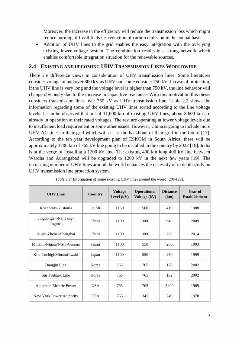
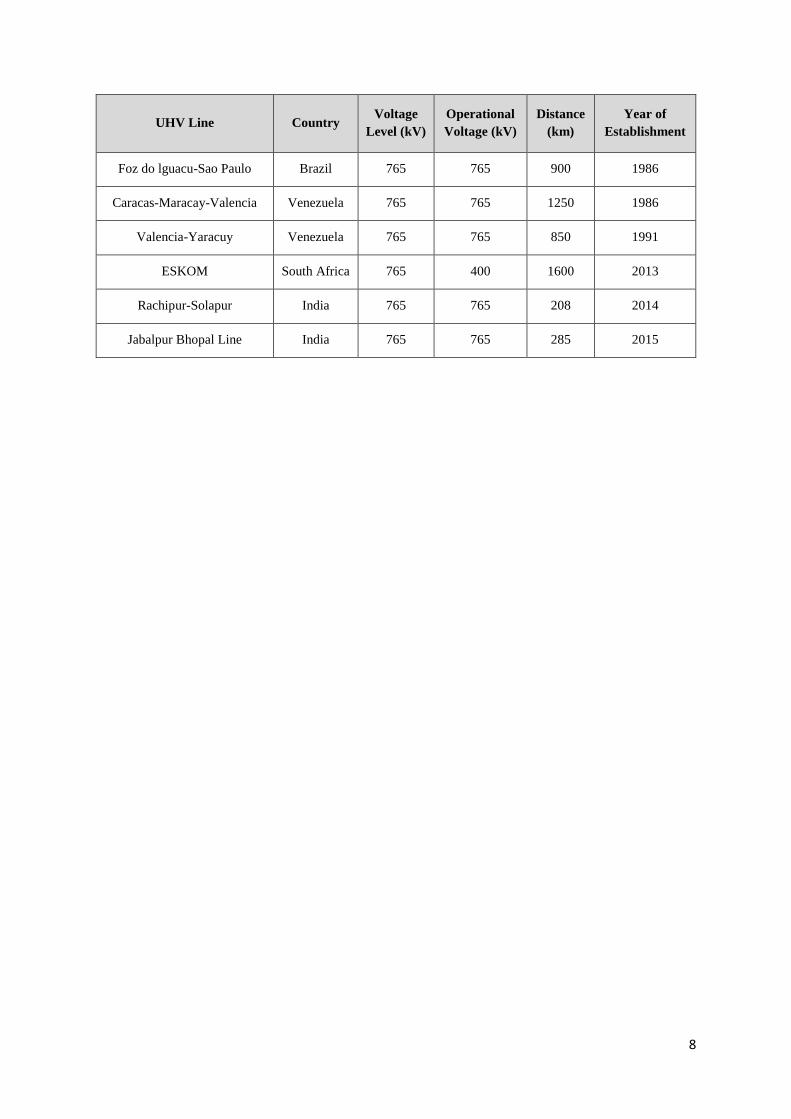
considers transmission lines over 750 kV as UHV transmission line. Table 2.2 shows the
information regarding some of the existing UHV lines sorted according to the line voltage
levels. It can be observed that out of 11,000 km of existing UHV lines, about 8,600 km are
already in operation at their rated voltages. The rest are operating at lower voltage levels due
to insufficient load requirement or some other issues. However, China is going to include more
UHV AC lines in their grid which will act as the backbone of their grid in the future [17].
According to the ten year development plan of ESKOM in South Africa, there will be
approximately 3700 km of 765 kV line going to be installed in the country by 2022 [18]. India
is at the verge of installing a 1200 kV line. The existing 400 km long 400 kV line between
Wardha and Aurangabad will be upgraded to 1200 kV in the next few years [19]. The
increasing number of UHV lines around the world enhances the necessity of in depth study on
UHV transmission line protection system.
Table 2.2: Information of some existing UHV lines around the world [20]–[29].
UHV Line Country Voltage
Level (kV)
Operational
Voltage (kV)
Distance
(km)
Year of
Establishment
Kokchetav-kustanai USSR 1150 500 410 1988
Jingdongan-Nanyang-
Jingmen China 1100 1000 640 2009
Huain-Zhebei-Shanghai China 1100 1000 780 2014
Minami-Nigata/Nishi-Gunma Japan 1100 550 200 1993
Kita-Tochigi/Minami-lwaki Japan 1100 550 250 1999
Dangjin Line Korea 765 765 178 2002
Sin Taebaek Line Korea 765 765 162 2002
American Electric Power USA 765 765 3400 1969
New York Power Authority USA 765 345 249 1978
8
UHV Line Country Voltage
Level (kV)
Operational
Voltage (kV)
Distance
(km)
Year of
Establishment
Foz do lguacu-Sao Paulo Brazil 765 765 900 1986
Caracas-Maracay-Valencia Venezuela 765 765 1250 1986
Valencia-Yaracuy Venezuela 765 765 850 1991
ESKOM South Africa 765 400 1600 2013
Rachipur-Solapur India 765 765 208 2014
Jabalpur Bhopal Line India 765 765 285 2015
9
Chapter 3
UHV Transmission line modelling
3 NEED FOR LINE MODEL
The accurate measurement of the fault currents, voltages and the impedance is of primary
importance for the proper operation of the power system protection to detect faults along the
lines and to locate the zones.
In general, the transmission line can be either represented as distributed parameter model or
lumped line model depending on the length of a line. A lumped line model with the impedances
of the entire line is assumed by multiplying the series impedance per unit length for most of
short lines. Also the fault current and impedance values calculated are based on this simple
model.
3.1 CHOICE OF THE MODEL
In case of a long Ultra High Voltage (UHV) transmission line, the lumped parameter model is
less useful, due to the effect of shunt capacitance distributed over the entire line together with
corona effect around the conductor. In an UHV line, the transmitted power is increased with
the reduction in the characteristic impedance of the line with the increase in the distributed
capacitance effect. Thus the losses in the line along with corona losses and the electric field
strength constraints are accounted [30]. In order to study the transient behaviour of UHV
transmission lines, an accurate model of the power system transmission network is necessary.
In the lumped parameter modelling, the transmission line is represented by resistance,
inductance and a parallel capacitance. The modelling is developed in the time domain.
A Pi model can be used to represent the long transmission line. Though the impedance of the
line is represented, it is only effective for the fundamental component while the frequencies
other than fundamental are not represented accurately. On the other hand, PI model cannot
reflect the transient signal transmission along the line because it is not frequency dependent
with distributed parameters and it could not create travelling wave reflections together with its
time delays. On the other hand, the frequency dependent model is developed by distributed
parameters of the line in frequency domain. All the simulations with frequency dependent
model is carried out in the frequency domain. It is analysed in [31] & [32] that the error caused
in the estimation of the fault distance calculation with the lumped parameter line model
accounts to 17%.
3.1.1 Frequency dependent line model
The frequency dependent model of transmission line used for modelling the UHV lines in
PSCAD is obtained based on the theory proposed in [33].
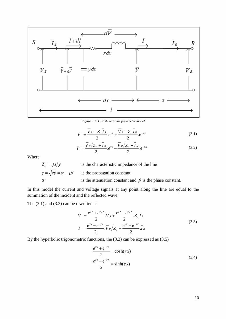
UHV power transmission is associated with long distance transmission and the representation
of the longline model with distributed parameters is presented in Figure 3.1. Considering the
longline model with transposition, the voltage and current relationships can be obtained (3.1)
and (3.2).
10
Figure 3.1: Distributed Line parameter model
. .2 2
R RR Rx xc cV Z I V Z IV e e
(3.1)
. .2 2
R RR Rx xc cV Z I V Z II e e (3.2)
Where,
cZ z y is the characteristic impedance of the line
zy j is the propagation constant.
is the attenuation constant and is the phase constant.
In this model the current and voltage signals at any point along the line are equal to the
summation of the incident and the reflected wave.
The (3.1) and (3.2) can be rewritten as
. .2 2
. .2 2
x x x x
RR c
x x x x
RR c
e e e eV V Z I
e e e eI V Z I
(3.3)
By the hyperbolic trigonometric functions, the (3.3) can be expressed as (3.5)
cosh( )2
sinh( )2
x x
x x
e ex
e ex
(3.4)
11
cosh sinh
cosh sinh
RR c
R R c
V V x Z I x
I I x V Z x
(3.5)
For the case of a lossless line,
cZ L C
j LC
(3.6)
From (3.6), the expression (3.5) can be written as (3.7) & (3.8)
.cos( ) .sin( )RR cV V x jZ I x (3.7)
.cos( ) / .sin( )R R cI I x j V Z x (3.8)
The frequency dependency is considered with distributed R, L and C parameters along the line
modelled as travelling waves. Also the parameters modelled represent the frequency
dependence. In the studies for the line characteristics for the UHV lines, the transient behaviour
is considered. In this consideration, the frequency dependent model is the most suited model,
as it gives an accurate representation of all frequencies. They can be simulated either by modal
techniques (Mode model) or phase domain techniques (phase model).
3.2 LINE MODEL IN PSCAD
In order to simulate the real time application of the UHV transmission system, various data
were analysed from the practical cases of UHV transmission around the world. The parameters
thus obtained are used in the modelling of the UHV line in PSCAD.
In this case, the 765 kV simulation system is chosen for the detailed study and simulation
purposes. The line is represented as a frequency dependent model in order to obtain the
information of all the frequency components during the transient state (faults). In line with the
transmission line frequency dependent model, the parameters for tower configuration,
conductor data, ground wire data are to be provided in PSCAD. All the data obtained from
different sources were compared and validated with the typical data and practical data [34]. In
this section both the values and the calculated parameters used in PSCAD model are discussed.
3.2.1 Type of conductors
After thorough investigation of different 765 kV transmission lines operated in countries like
China, India, Japan, South Korea and USA, it is observed that the conductors used in UHV
transmission lines are cardinal, curlew or rail.
Owing to the minimum resistance of the conductor and the higher ampere capacity, Cardinal
54/7 is chosen for the studies. Table 3.1 shows the typical conductor characteristics. For UHV
lines the power transmitted is high and a bundled conductor is considered in this case. The
cardinal 54/7 conductor is in practical usage in the Korea Electric Power Company (KEPCO)
765kV transmission lines [35].
Advantages of having a bundle will reduce the losses in the line and the skin effect and the
corona.
12
The 765kV lines are in general designed for a power rating of more than 4000MVA
transmission capacity. In line with the theory and the standard practice, a transmission line with
a 6 sub-conductor bundle is considered
The maximum power transmission in the 765kV line is calculated as 8000 MVA considering
the 6 conductors with 996 A current capacity and it is given by (3.9) below
3. 3 996 6 765
8000
S IV
S MVA
(3.9)
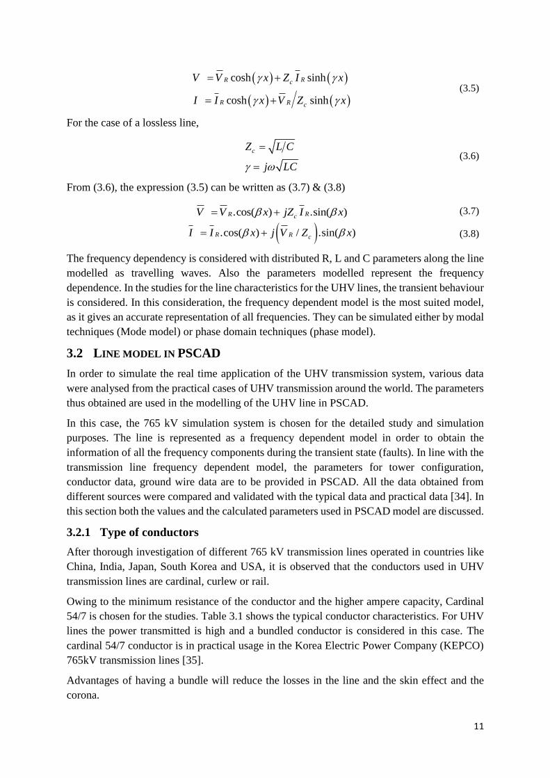
The transmission line towers are available in PSCAD line model library.
The tower components are used to define the geometric configuration of the transmission line.
The configuration editor for the overhead line towers consider the input parameter description
for tower data, circuit conductor data, circuit ground data. The following Figure 3.2 provides
the information of the line geometry used in modelling the UHV transmission line in PSCAD.
As it can be seen from the Figure 3.2 that a three phase line model is arranged in a triangular
configuration with equally spaced distance of 14 m.
Figure 3.2: line geometry
The line is considered ideally transposed and considered with 2 ground wires. The circuit
conductor data includes the geometric mean radius of the conductor which is the individual
radius ('r ) of each sub conductor in the bundle. Each phase has 6 bundled conductors which
have been selected based on most practical 765 kV line parameters. The value 'r for the sub
conductor is calculated as (3.10)
Individual sub- conductor diameter = 1.196 inch [36]
Considering the conversion factor in meters,
Diameter =0.03078 m
13
(1/4)
(1/4)
'
'
.2
0.03048.
2
0.0119857
diametere
e
m
r
r
(3.10)
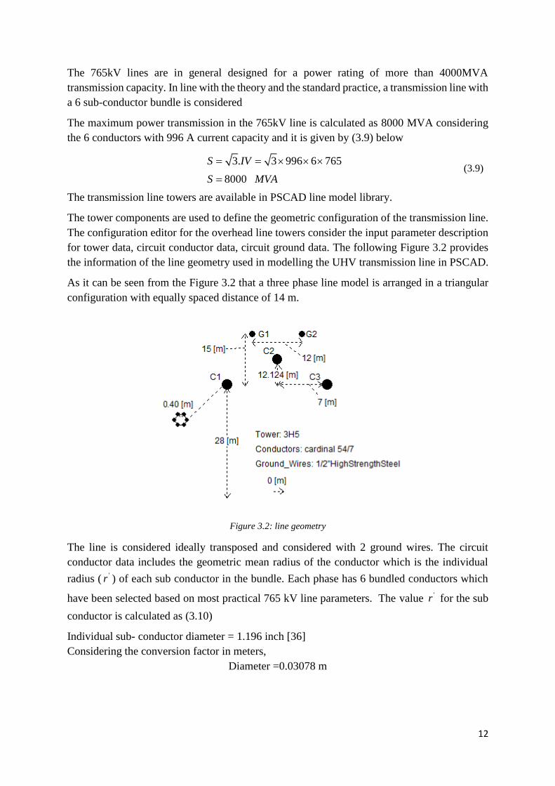
The conductor and ground wire parameters used for the model of the line is presented in Table
3.1 for reference. The values in the table are obtained by calculation based on the data provided
in PSCAD
Table 3.1: Conductor parameters used for UHV line model
Parameter Data used
Sub -Conductor
Radius 'r (m)
0.0119857
Conductor DC
Resistance (ohm/km) 0.058727
Ground Wire radius 0.0055245
Ground wire DC resistance 2.5
3.2.2 Surge Impedance loading
In the UHV lines the value of R is small and negligible, and the line is assumed to be lossless
subject to high voltage surges. The impedance associated with the line without losses and
resistance effect is called surge impedance and the power transmitted through the line is called
surge impedance loading (SIL) given by (3.12).
CZ L C (3.11)
2
0
C
VSIL W
Z (3.12)
Where, 0V is the rated line voltage.
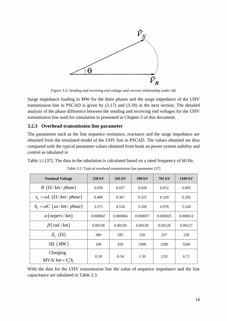
At SIL, it is observed that
1. The voltage and current at the sending and receiving end are constant and equal in
amplitude.
2. Voltage and current signals are in phase along the line length.
3. There is a phase shift between the sending end and receiving voltage signals, owing to
the length of transmission lines. This phase difference is given by l . Where, is the
phase constant and l is the line length.
The phase shift between the sending end and receiving end parameters is a phenomenon due to
the long transmission line and it is not due to UHV. But UHV lines are associated with long
distance power transmission and it is significant to observe.
14
Figure 3.3: Sending and receiving end voltage and current relationship under SIL
Surge impedance loading in MW for the three phases and the surge impedance of the UHV
transmission line in PSCAD is given by (3.17) and (3.18) in the next section. The detailed
analysis of the phase difference between the sending and receiving end voltages for the UHV
transmission line used for simulation in presented in Chapter-3 of this document.
3.2.3 Overhead transmission line parameter
The parameters such as the line sequence resistance, reactance and the surge impedance are
obtained from the simulated model of the UHV line in PSCAD. The values obtained are thus
compared with the typical parameter values obtained from book on power system stability and
control as tabulated in
Table 3.2 [37]. The data in the tabulation is calculated based on a rated frequency of 60 Hz.
Table 3.2: Typical overhead transmission line parameter [37]
With the data for the UHV transmission line the value of sequence impedance and the line
capacitance are tabulated in Table 3.3.
Nominal Voltage 230 kV 345 kV 500 kV 765 kV 1100 kV
/ /R km phase
0.050 0.037 0.028 0.012 0.005
/ /Lx L km phase
0.488 0.367 0.325 0.329 0.292
/ /Cb C us km phase
3.371 4.518 5.200 4.978 5.544
/nepers km
0.000067 0.000066 0.000057 0.000025 0.000012
/rad km
0.00128 0.00129 0.00130 0.00128 0.00127
CZ
380 285 250 257 230
SIL MW
140 420 1000 2280 5260
2
0
Charging
MVA/ ckm V b 0.18 0.54 1.30 2.92 6.71
15
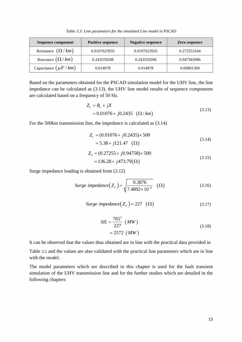
Table 3.3: Line parameters for the simulated Line model in PSCAD
Sequence component Positive sequence Negative sequence Zero sequence
Resistance / km 0.0107623935 0.0107623935 0.272553164
Reactance / km 0.243559208 0.243559208 0.947583086
Capacitance /F km 0.014978 0.014978 0.00891309
Based on the parameters obtained for the PSCAD simulation model for the UHV line, the line
impedance can be calculated as (3.13). the UHV line model results of sequence components
are calculated based on a frequency of 50 Hz.
1 1
0.01076 0.2435 /
Z R jX
j km
(3.13)
For the 500km transmission line, the impedance is calculated as (3.14)
1 (0.01076 0.2435) 500
5.38 121.47
Z j
j
(3.14)
0 ( 0 ) 500. 02725
136.28 473.7
5 .94758
9
Z j
j
(3.15)
Surge impedance loading is obtained from (3.12)
6
0.3876
7.4892 10CSurge impedance Z
(3.16)
227CSurge impedance Z (3.17)
2765
227
2572
SIL MW
MW
(3.18)
It can be observed that the values thus obtained are in line with the practical data provided in
Table 3.2 and the values are also validated with the practical line parameters which are in line
with the model.
The model parameters which are described in this chapter is used for the fault transient
simulation of the UHV transmission line and for the further studies which are detailed in the
following chapters
16
Chapter 4
Features of UHV transmission systems
4 ANALYSIS OF TYPICAL FEATURES OF UHV TRANSMISSION
SYSTEMS
The UHV power transmission technology is of great importance as it attracts the power utilities
with its higher power transmission capacity over long distances. In this regards, it also poses a
number of challenges with regards to the system protection, overvoltage during switching,
capacitive leakage currents and harmonic effects. In this report fault transient in UHV power
system transmission is analysed.
Also the distance protection scheme related impedance measurement is mainly analysed during
fault transient and detailed analysis of its influence in protection will be described in the later
chapters.
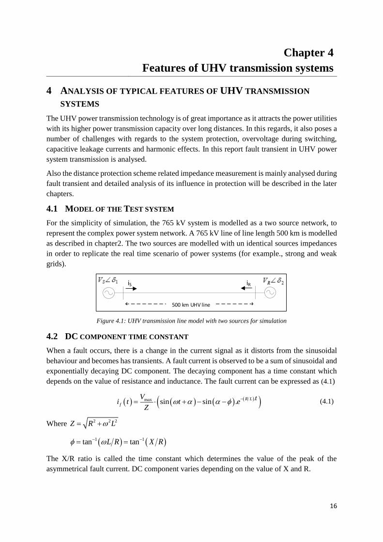
4.1 MODEL OF THE TEST SYSTEM
For the simplicity of simulation, the 765 kV system is modelled as a two source network, to
represent the complex power system network. A 765 kV line of line length 500 km is modelled
as described in chapter2. The two sources are modelled with un identical sources impedances
in order to replicate the real time scenario of power systems (for example., strong and weak
grids).
Figure 4.1: UHV transmission line model with two sources for simulation
4.2 DC COMPONENT TIME CONSTANT
When a fault occurs, there is a change in the current signal as it distorts from the sinusoidal
behaviour and becomes has transients. A fault current is observed to be a sum of sinusoidal and
exponentially decaying DC component. The decaying component has a time constant which
depends on the value of resistance and inductance. The fault current can be expressed as (4.1)
.max sin sin .R L
f
tVi t t e
Z
(4.1)
Where 2 2 2Z R L
1 1tan tanL R X R
The X/R ratio is called the time constant which determines the value of the peak of the
asymmetrical fault current. DC component varies depending on the value of X and R.
iS iR
500 km UHV line
17
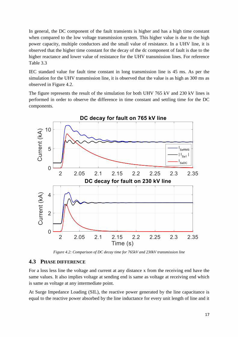
In general, the DC component of the fault transients is higher and has a high time constant
when compared to the low voltage transmission system. This higher value is due to the high
power capacity, multiple conductors and the small value of resistance. In a UHV line, it is
observed that the higher time constant for the decay of the dc component of fault is due to the
higher reactance and lower value of resistance for the UHV transmission lines. For reference
Table 3.3
IEC standard value for fault time constant in long transmission line is 45 ms. As per the
simulation for the UHV transmission line, it is observed that the value is as high as 300 ms as
observed in Figure 4.2.
The figure represents the result of the simulation for both UHV 765 kV and 230 kV lines is
performed in order to observe the difference in time constant and settling time for the DC
components.
Figure 4.2: Comparison of DC decay time for 765kV and 230kV transmission line
4.3 PHASE DIFFERENCE
For a loss less line the voltage and current at any distance x from the receiving end have the
same values. It also implies voltage at sending end is same as voltage at receiving end which
is same as voltage at any intermediate point.
At Surge Impedance Loading (SIL), the reactive power generated by the line capacitance is
equal to the reactive power absorbed by the line inductance for every unit length of line and it
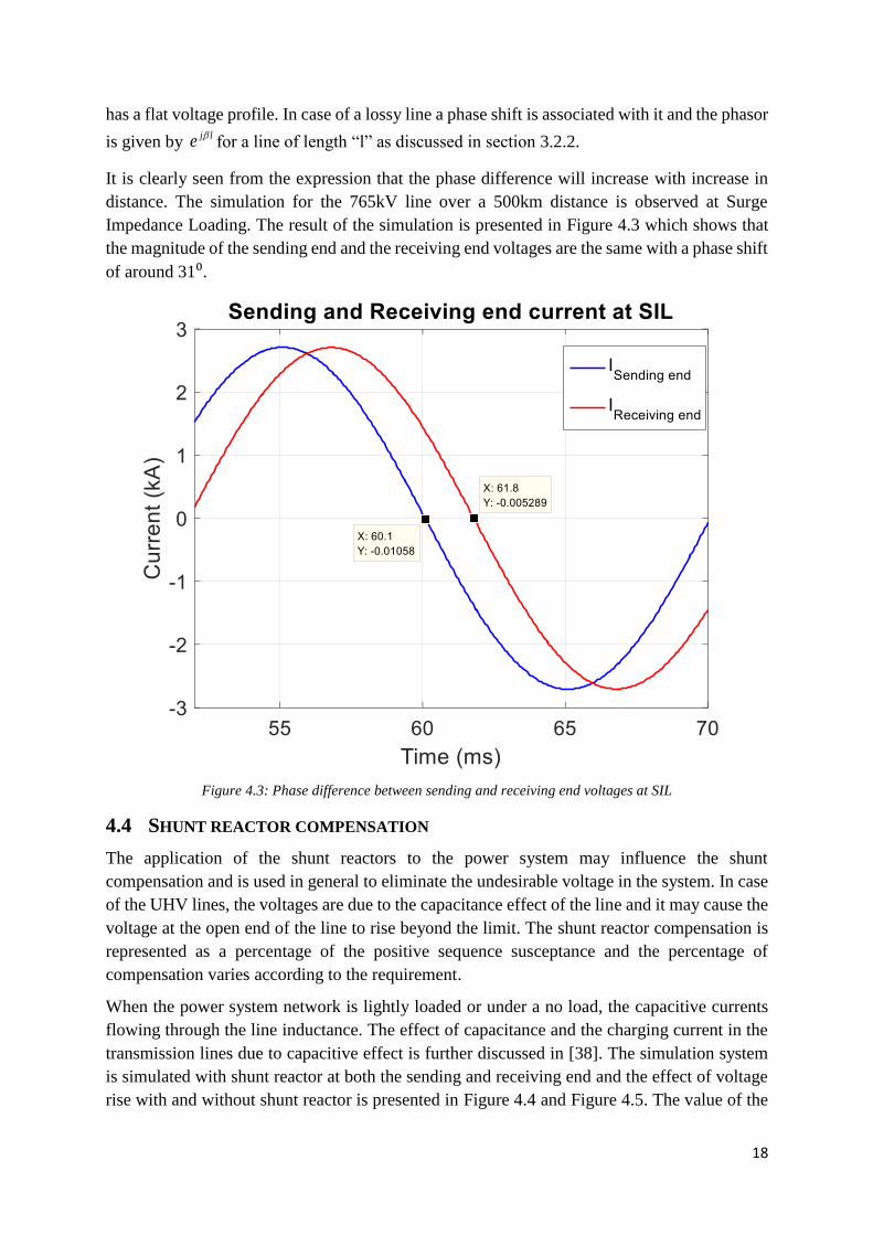
18
has a flat voltage profile. In case of a lossy line a phase shift is associated with it and the phasor
is given by j le
for a line of length “l” as discussed in section 3.2.2.
It is clearly seen from the expression that the phase difference will increase with increase in
distance. The simulation for the 765kV line over a 500km distance is observed at Surge
Impedance Loading. The result of the simulation is presented in Figure 4.3 which shows that
the magnitude of the sending end and the receiving end voltages are the same with a phase shift
of around 31⁰.
Figure 4.3: Phase difference between sending and receiving end voltages at SIL
4.4 SHUNT REACTOR COMPENSATION
The application of the shunt reactors to the power system may influence the shunt
compensation and is used in general to eliminate the undesirable voltage in the system. In case
of the UHV lines, the voltages are due to the capacitance effect of the line and it may cause the
voltage at the open end of the line to rise beyond the limit. The shunt reactor compensation is
represented as a percentage of the positive sequence susceptance and the percentage of
compensation varies according to the requirement.
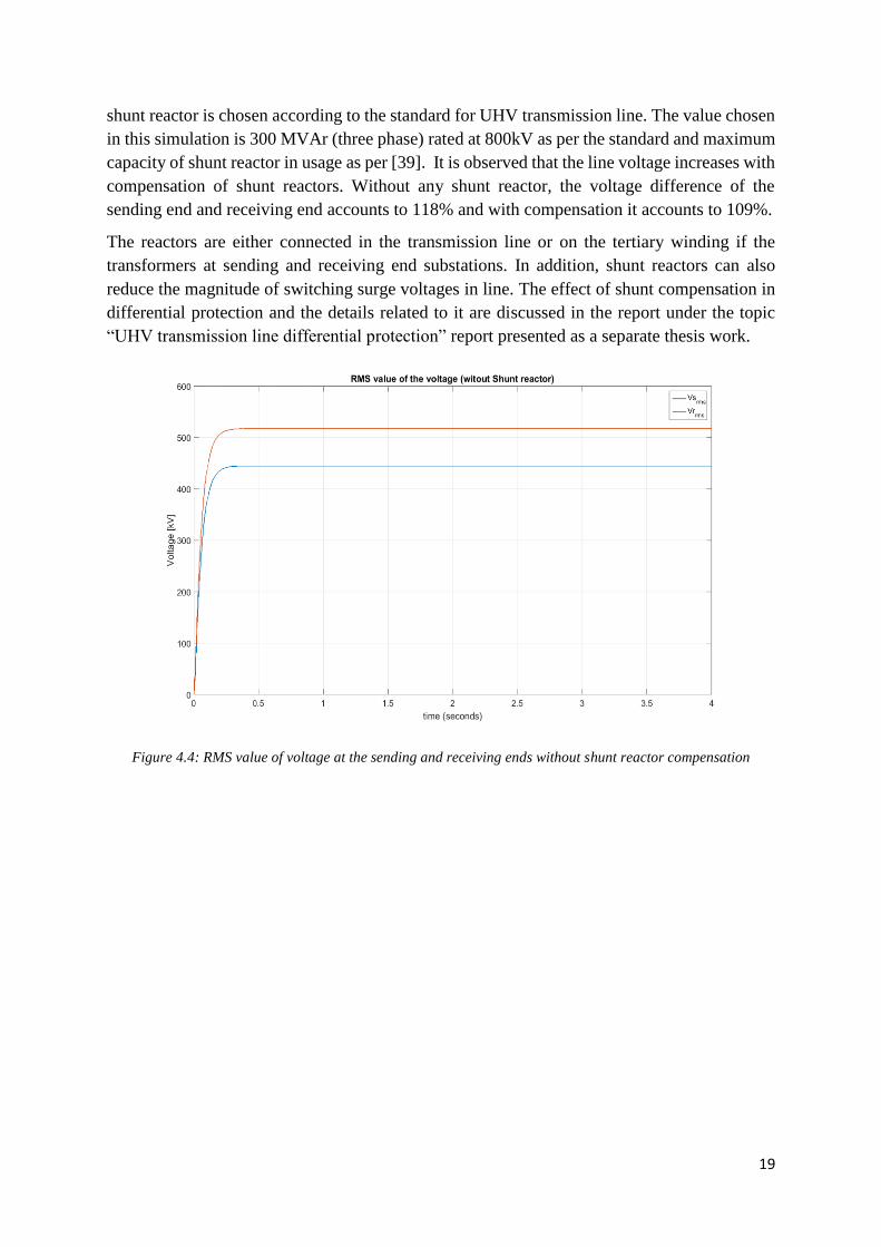
When the power system network is lightly loaded or under a no load, the capacitive currents
flowing through the line inductance. The effect of capacitance and the charging current in the
transmission lines due to capacitive effect is further discussed in [38]. The simulation system
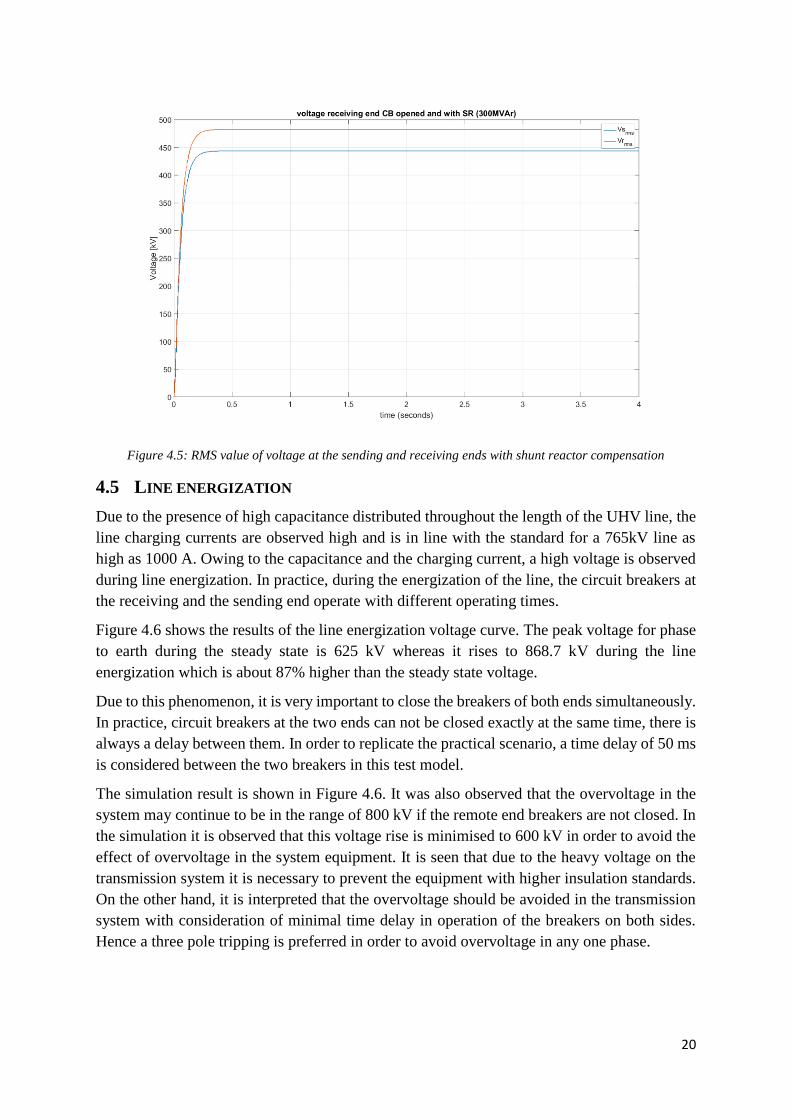
is simulated with shunt reactor at both the sending and receiving end and the effect of voltage
rise with and without shunt reactor is presented in Figure 4.4 and Figure 4.5. The value of the
19
shunt reactor is chosen according to the standard for UHV transmission line. The value chosen
in this simulation is 300 MVAr (three phase) rated at 800kV as per the standard and maximum
capacity of shunt reactor in usage as per [39]. It is observed that the line voltage increases with
compensation of shunt reactors. Without any shunt reactor, the voltage difference of the
sending end and receiving end accounts to 118% and with compensation it accounts to 109%.
The reactors are either connected in the transmission line or on the tertiary winding if the
transformers at sending and receiving end substations. In addition, shunt reactors can also
reduce the magnitude of switching surge voltages in line. The effect of shunt compensation in
differential protection and the details related to it are discussed in the report under the topic
“UHV transmission line differential protection” report presented as a separate thesis work.
Figure 4.4: RMS value of voltage at the sending and receiving ends without shunt reactor compensation
20
Figure 4.5: RMS value of voltage at the sending and receiving ends with shunt reactor compensation
4.5 LINE ENERGIZATION
Due to the presence of high capacitance distributed throughout the length of the UHV line, the
line charging currents are observed high and is in line with the standard for a 765kV line as
high as 1000 A. Owing to the capacitance and the charging current, a high voltage is observed
during line energization. In practice, during the energization of the line, the circuit breakers at
the receiving and the sending end operate with different operating times.
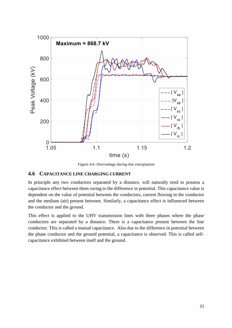
Figure 4.6 shows the results of the line energization voltage curve. The peak voltage for phase
to earth during the steady state is 625 kV whereas it rises to 868.7 kV during the line
energization which is about 87% higher than the steady state voltage.
Due to this phenomenon, it is very important to close the breakers of both ends simultaneously.
In practice, circuit breakers at the two ends can not be closed exactly at the same time, there is
always a delay between them. In order to replicate the practical scenario, a time delay of 50 ms
is considered between the two breakers in this test model.
The simulation result is shown in Figure 4.6. It was also observed that the overvoltage in the
system may continue to be in the range of 800 kV if the remote end breakers are not closed. In
the simulation it is observed that this voltage rise is minimised to 600 kV in order to avoid the
effect of overvoltage in the system equipment. It is seen that due to the heavy voltage on the
transmission system it is necessary to prevent the equipment with higher insulation standards.
On the other hand, it is interpreted that the overvoltage should be avoided in the transmission
system with consideration of minimal time delay in operation of the breakers on both sides.
Hence a three pole tripping is preferred in order to avoid overvoltage in any one phase.
21
Figure 4.6: Overvoltage during line energization
4.6 CAPACITANCE LINE CHARGING CURRENT
In principle any two conductors separated by a distance, will naturally tend to possess a
capacitance effect between them owing to the difference in potential. This capacitance value is
dependent on the value of potential between the conductors, current flowing in the conductor
and the medium (air) present between. Similarly, a capacitance effect is influenced between
the conductor and the ground.
This effect is applied to the UHV transmission lines with three phases where the phase
conductors are separated by a distance. There is a capacitance present between the line
conductor. This is called a mutual capacitance. Also due to the difference in potential between
the phase conductor and the ground potential, a capacitance is observed. This is called self-
capacitance exhibited between itself and the ground.
22
ACC
ABC BC
C
AGC
BGC
CGC
A CB
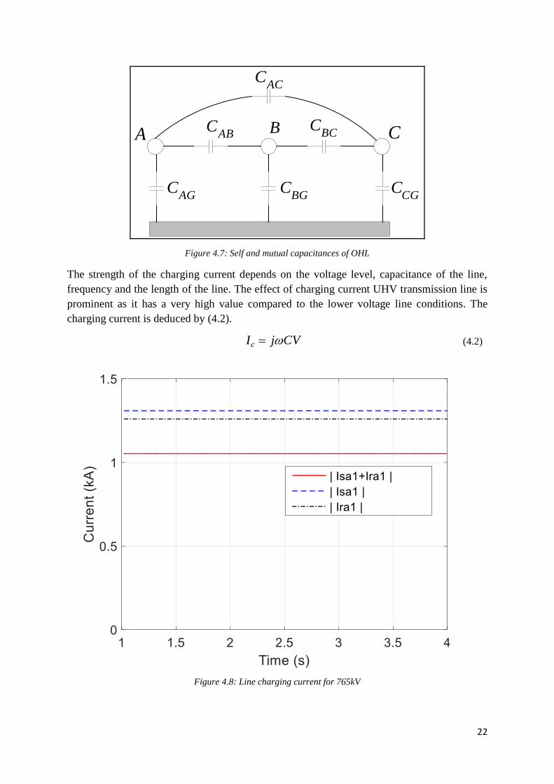
Figure 4.7: Self and mutual capacitances of OHL
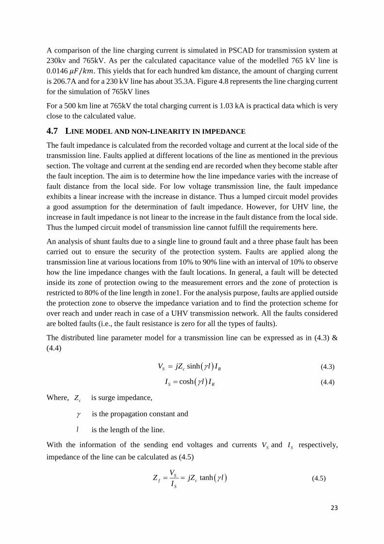
The strength of the charging current depends on the voltage level, capacitance of the line,
frequency and the length of the line. The effect of charging current UHV transmission line is
prominent as it has a very high value compared to the lower voltage line conditions. The
charging current is deduced by (4.2).
cI j CV (4.2)
Figure 4.8: Line charging current for 765kV
23
A comparison of the line charging current is simulated in PSCAD for transmission system at
230kv and 765kV. As per the calculated capacitance value of the modelled 765 kV line is
0.0146 𝜇𝐹/𝑘𝑚. This yields that for each hundred km distance, the amount of charging current
is 206.7A and for a 230 kV line has about 35.3A. Figure 4.8 represents the line charging current
for the simulation of 765kV lines
For a 500 km line at 765kV the total charging current is 1.03 kA is practical data which is very
close to the calculated value.
4.7 LINE MODEL AND NON-LINEARITY IN IMPEDANCE
The fault impedance is calculated from the recorded voltage and current at the local side of the
transmission line. Faults applied at different locations of the line as mentioned in the previous
section. The voltage and current at the sending end are recorded when they become stable after
the fault inception. The aim is to determine how the line impedance varies with the increase of
fault distance from the local side. For low voltage transmission line, the fault impedance
exhibits a linear increase with the increase in distance. Thus a lumped circuit model provides
a good assumption for the determination of fault impedance. However, for UHV line, the
increase in fault impedance is not linear to the increase in the fault distance from the local side.
Thus the lumped circuit model of transmission line cannot fulfill the requirements here.
An analysis of shunt faults due to a single line to ground fault and a three phase fault has been
carried out to ensure the security of the protection system. Faults are applied along the
transmission line at various locations from 10% to 90% line with an interval of 10% to observe
how the line impedance changes with the fault locations. In general, a fault will be detected
inside its zone of protection owing to the measurement errors and the zone of protection is
restricted to 80% of the line length in zone1. For the analysis purpose, faults are applied outside
the protection zone to observe the impedance variation and to find the protection scheme for
over reach and under reach in case of a UHV transmission network. All the faults considered
are bolted faults (i.e., the fault resistance is zero for all the types of faults).
The distributed line parameter model for a transmission line can be expressed as in (4.3) &
(4.4)
sinhS c RV jZ l I (4.3)
coshS RI l I (4.4)
Where, cZ is surge impedance,
is the propagation constant and
l is the length of the line.
With the information of the sending end voltages and currents SV and SI respectively,
impedance of the line can be calculated as (4.5)
tanhSf c
S
VZ jZ l
I
(4.5)
24
The impedance along the line for various locations is calculated and plotted in comparison with
the fault impedance calculated from different shunt faults.
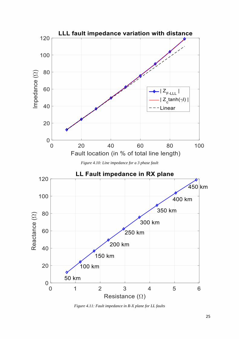
Figure 4.10 shows that the fault impedance for a three phase to ground bolted faults varies
according to the equation mentioned above. It is also visible that the increase of fault impedance
is not linear to the increase in the distance of fault locations. This characteristic makes the fault
detection at boundary of zone 1 in the distance protection very critical.
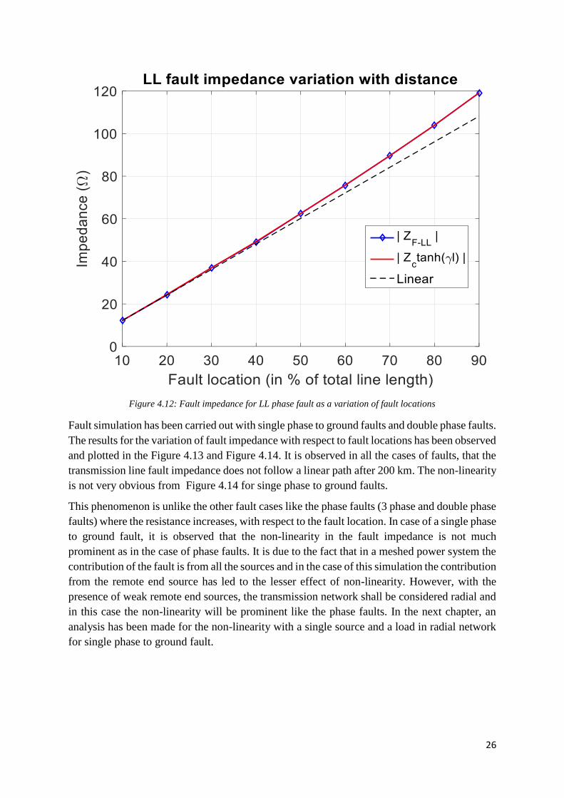
The analysis is carried out for double phase faults and the results are plotted in Figure 4.11 and
Figure 4.12. It is observed that the double phase fault shows similar characteristics like a three
phase fault.
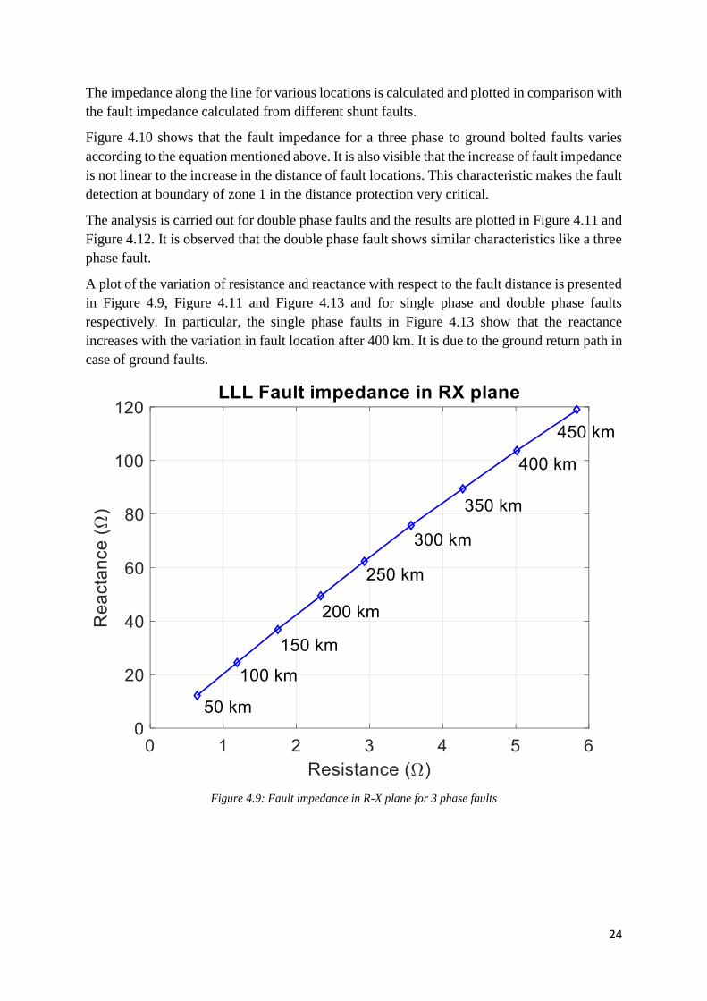
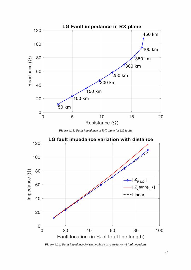
A plot of the variation of resistance and reactance with respect to the fault distance is presented
in Figure 4.9, Figure 4.11 and Figure 4.13 and for single phase and double phase faults
respectively. In particular, the single phase faults in Figure 4.13 show that the reactance
increases with the variation in fault location after 400 km. It is due to the ground return path in
case of ground faults.
Figure 4.9: Fault impedance in R-X plane for 3 phase faults
25
Figure 4.10: Line impedance for a 3 phase fault
Figure 4.11: Fault impedance in R-X plane for LL faults
26
Figure 4.12: Fault impedance for LL phase fault as a variation of fault locations
Fault simulation has been carried out with single phase to ground faults and double phase faults.
The results for the variation of fault impedance with respect to fault locations has been observed
and plotted in the Figure 4.13 and Figure 4.14. It is observed in all the cases of faults, that the
transmission line fault impedance does not follow a linear path after 200 km. The non-linearity
is not very obvious from Figure 4.14 for singe phase to ground faults.
This phenomenon is unlike the other fault cases like the phase faults (3 phase and double phase
faults) where the resistance increases, with respect to the fault location. In case of a single phase
to ground fault, it is observed that the non-linearity in the fault impedance is not much
prominent as in the case of phase faults. It is due to the fact that in a meshed power system the
contribution of the fault is from all the sources and in the case of this simulation the contribution
from the remote end source has led to the lesser effect of non-linearity. However, with the
presence of weak remote end sources, the transmission network shall be considered radial and
in this case the non-linearity will be prominent like the phase faults. In the next chapter, an
analysis has been made for the non-linearity with a single source and a load in radial network
for single phase to ground fault.
27
Figure 4.13: Fault impedance in R-X plane for LG faults
Figure 4.14: Fault impedance for single phase as a variation of fault locations
28
Chapter 5
Fault analysis and impacts of UHV transmission line
5 FAULT IMPEDANCE TRANSIENTS
The test model of the UHV transmission system is analysed to study the transient behaviour
and the challenges it possesses. In this case, the transmission line fault transients are studied
and its impact on the existing protection schemes are analysed and discussed. In this chapter,
the different types of faults in the transmission system along with the UHV transients are
presented in detail.
Transmission lines are important aspect in a power system, since the lines link to adjacent lines
and equipment. Any interruption in the line and faults on the line will adversely affect the
system. Hence it is required to protect the transmission line during the fault transients in line
with the other protection of the other connected equipment in power system.
In principle a protection scheme should be able to detect the abnormalities in the operation of
the power system and to protect the system from damage. A relay is a device that should be
able to perform this action by evaluating the various parameters to achieve the system
protection. The voltage and current signals at the transmission line terminals are the common
parameters. The relay must be able to detect the normal conditions and fault transients in order
to attain the security of the system. There are many protection schemes opted for the protection
of a transmission line namely, distance, differential, overcurrent, etc.,
Distance protection is one of the main protection schemes used in power system owing to its
high speed of fault clearance and sensitivity. The distance protection scheme is based on the
impedance of the transmission line and the location if the fault distance based on the value of
the fault impedance in comparison with the total line impedance.
5.1 FAULT TRANSIENTS AND ITS TYPES
In a typical power system network, faults can be broadly classified as series and shunt faults.
A series fault may be due to an open circuit in line because of a broken conductor or due to
failure of a circuit breaker. The shunt faults are also called short circuit faults are due to the
insulation failure, lightening surges, overloading or breakdown of transmission line, etc.,
The shunt faults can be classified as symmetrical and unsymmetrical faults depending on the
nature of the fault. Symmetric faults are balanced faults and it affects all the three phases of the
power system network which is a three phase to ground fault or a three phase fault (LLLG).
Most fault in power system is asymmetric or unbalanced faults and it affects only specific
phases of the power system which are single phase to ground fault (LG), double phase to
ground fault (LLG) and double phase fault (LL). As per [40], single phase to ground fault is
the most frequently occurring faults in a power system. A tabulation for the probability of
occurrence of different faults in a power system is presented in Table 5.1.
In this thesis report focus on the different types of shunt faults in the transmission line for the
purpose of analysis and the challenges it poses in a distance relaying scheme.
29
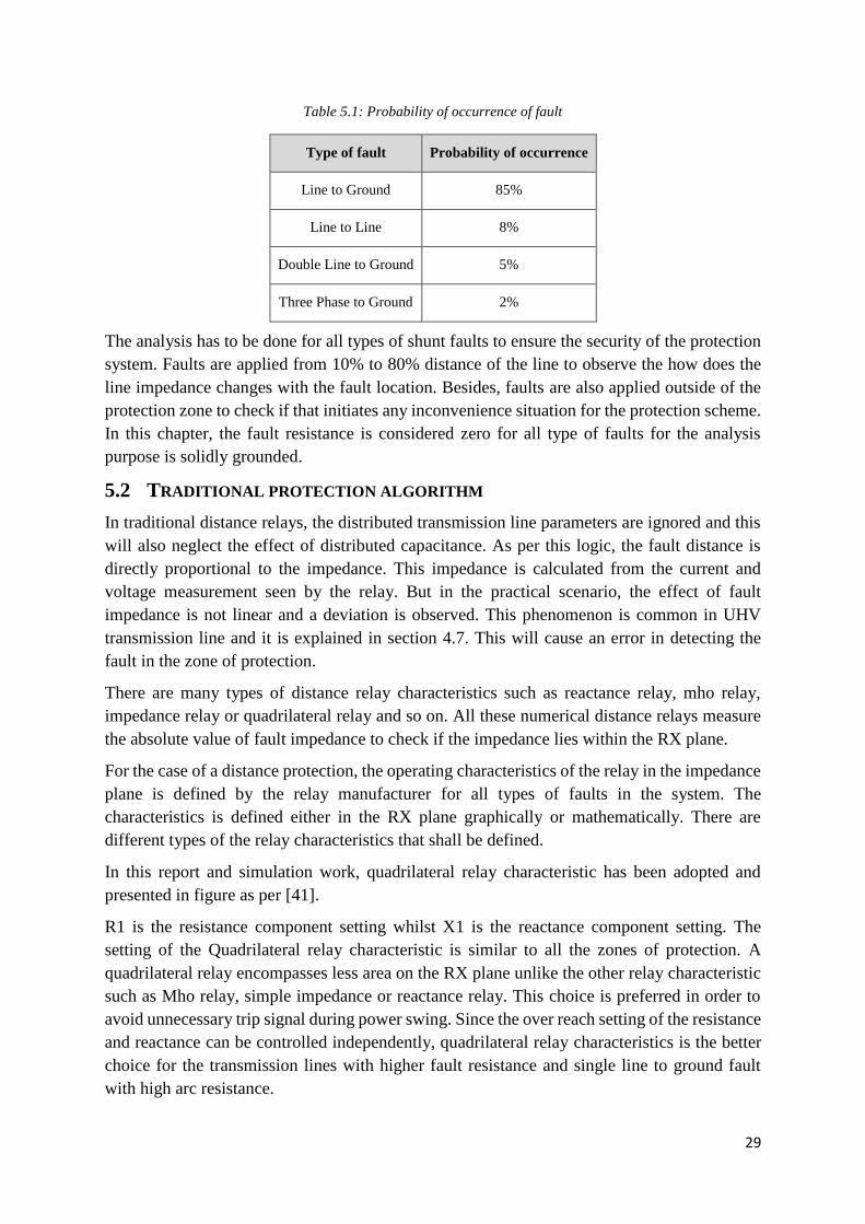
Table 5.1: Probability of occurrence of fault
Type of fault Probability of occurrence
Line to Ground 85%
Line to Line 8%
Double Line to Ground 5%
Three Phase to Ground 2%
The analysis has to be done for all types of shunt faults to ensure the security of the protection
system. Faults are applied from 10% to 80% distance of the line to observe the how does the
line impedance changes with the fault location. Besides, faults are also applied outside of the
protection zone to check if that initiates any inconvenience situation for the protection scheme.
In this chapter, the fault resistance is considered zero for all type of faults for the analysis
purpose is solidly grounded.
5.2 TRADITIONAL PROTECTION ALGORITHM
In traditional distance relays, the distributed transmission line parameters are ignored and this
will also neglect the effect of distributed capacitance. As per this logic, the fault distance is
directly proportional to the impedance. This impedance is calculated from the current and
voltage measurement seen by the relay. But in the practical scenario, the effect of fault
impedance is not linear and a deviation is observed. This phenomenon is common in UHV
transmission line and it is explained in section 4.7. This will cause an error in detecting the
fault in the zone of protection.
There are many types of distance relay characteristics such as reactance relay, mho relay,
impedance relay or quadrilateral relay and so on. All these numerical distance relays measure
the absolute value of fault impedance to check if the impedance lies within the RX plane.
For the case of a distance protection, the operating characteristics of the relay in the impedance
plane is defined by the relay manufacturer for all types of faults in the system. The
characteristics is defined either in the RX plane graphically or mathematically. There are
different types of the relay characteristics that shall be defined.
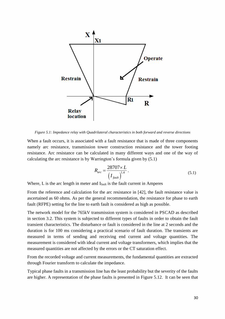
In this report and simulation work, quadrilateral relay characteristic has been adopted and
presented in figure as per [41].
R1 is the resistance component setting whilst X1 is the reactance component setting. The
setting of the Quadrilateral relay characteristic is similar to all the zones of protection. A
quadrilateral relay encompasses less area on the RX plane unlike the other relay characteristic
such as Mho relay, simple impedance or reactance relay. This choice is preferred in order to
avoid unnecessary trip signal during power swing. Since the over reach setting of the resistance
and reactance can be controlled independently, quadrilateral relay characteristics is the better
choice for the transmission lines with higher fault resistance and single line to ground fault
with high arc resistance.
30
Figure 5.1: Impedance relay with Quadrilateral characteristics in both forward and reverse directions
When a fault occurs, it is associated with a fault resistance that is made of three components
namely arc resistance, transmission tower construction resistance and the tower footing
resistance. Arc resistance can be calculated in many different ways and one of the way of
calculating the arc resistance is by Warrington’s formula given by (5.1)
1.4
28707arc
fault
LR
I
.
(5.1)
Where, L is the arc length in meter and Ifault is the fault current in Amperes
From the reference and calculation for the arc resistance in [42], the fault resistance value is
ascertained as 60 ohms. As per the general recommendation, the resistance for phase to earth
fault (RFPE) setting for the line to earth fault is considered as high as possible.
The network model for the 765kV transmission system is considered in PSCAD as described
in section 3.2. This system is subjected to different types of faults in order to obtain the fault
transient characteristics. The disturbance or fault is considered in the line at 2 seconds and the
duration is for 100 ms considering a practical scenario of fault duration. The transients are
measured in terms of sending and receiving end current and voltage quantities. The
measurement is considered with ideal current and voltage transformers, which implies that the
measured quantities are not affected by the errors or the CT saturation effect.
From the recorded voltage and current measurements, the fundamental quantities are extracted
through Fourier transform to calculate the impedance.
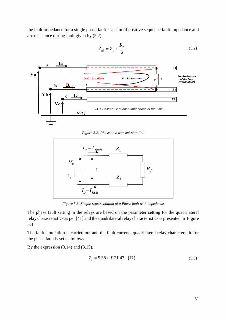
Typical phase faults in a transmission line has the least probability but the severity of the faults
are higher. A representation of the phase faults is presented in Figure 5.12. It can be seen that
31
the fault impedance for a single phase fault is a sum of positive sequence fault impedance and
arc resistance during fault given by (5.2).
1
2
f
ab
RZ Z (5.2)
Figure 5.2: Phase on a transmission line
a faultI I
1Z
fRV
aV
bV
b faultI I
1Z
Figure 5.3: Simple representation of a Phase fault with impedacne
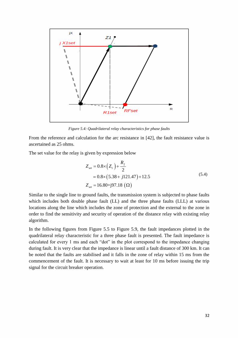
The phase fault setting in the relays are based on the parameter setting for the quadrilateral
relay characteristics as per [41] and the quadrilateral relay characteristics is presented in Figure
5.4
The fault simulation is carried out and the fault currents quadrilateral relay characteristic for
the phase fault is set as follows
By the expression (3.14) and (3.15),
1 5.38 121.47Z j (5.3)
32
Figure 5.4: Quadrilateral relay characteristics for phase faults
From the reference and calculation for the arc resistance in [42], the fault resistance value is
ascertained as 25 ohms.
The set value for the relay is given by expression below
10.82
0.8 5.38 121.47 12.5
16.80+j97.18
f
set
set
RZ Z
j
Z
(5.4)
Similar to the single line to ground faults, the transmission system is subjected to phase faults
which includes both double phase fault (LL) and the three phase faults (LLL) at various
locations along the line which includes the zone of protection and the external to the zone in
order to find the sensitivity and security of operation of the distance relay with existing relay
algorithm.
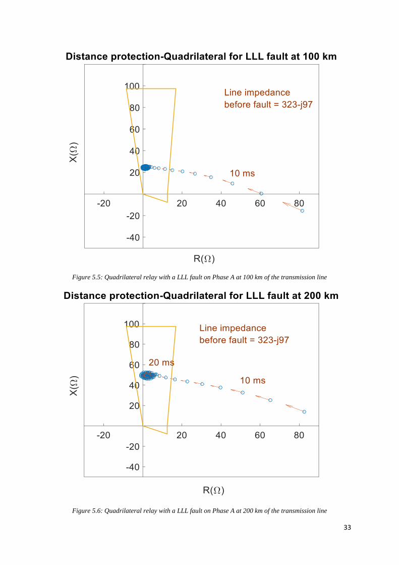
In the following figures from Figure 5.5 to Figure 5.9, the fault impedances plotted in the
quadrilateral relay characteristic for a three phase fault is presented. The fault impedance is
calculated for every 1 ms and each “dot” in the plot correspond to the impedance changing
during fault. It is very clear that the impedance is linear until a fault distance of 300 km. It can
be noted that the faults are stabilised and it falls in the zone of relay within 15 ms from the
commencement of the fault. It is necessary to wait at least for 10 ms before issuing the trip
signal for the circuit breaker operation.
33
Figure 5.5: Quadrilateral relay with a LLL fault on Phase A at 100 km of the transmission line
Figure 5.6: Quadrilateral relay with a LLL fault on Phase A at 200 km of the transmission line
34
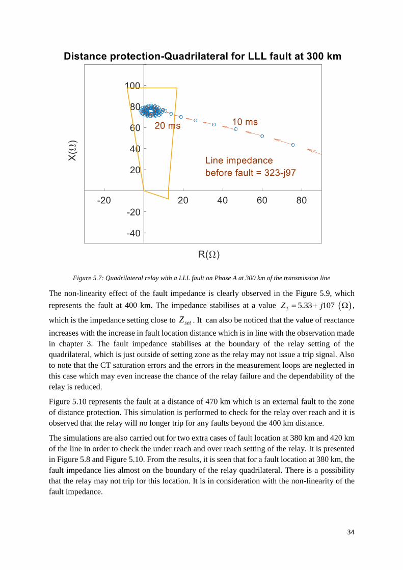
Figure 5.7: Quadrilateral relay with a LLL fault on Phase A at 300 km of the transmission line
The non-linearity effect of the fault impedance is clearly observed in the Figure 5.9, which
represents the fault at 400 km. The impedance stabilises at a value 5.33 107fZ j ,
which is the impedance setting close to setZ . It can also be noticed that the value of reactance
increases with the increase in fault location distance which is in line with the observation made
in chapter 3. The fault impedance stabilises at the boundary of the relay setting of the
quadrilateral, which is just outside of setting zone as the relay may not issue a trip signal. Also
to note that the CT saturation errors and the errors in the measurement loops are neglected in
this case which may even increase the chance of the relay failure and the dependability of the
relay is reduced.
Figure 5.10 represents the fault at a distance of 470 km which is an external fault to the zone
of distance protection. This simulation is performed to check for the relay over reach and it is
observed that the relay will no longer trip for any faults beyond the 400 km distance.
The simulations are also carried out for two extra cases of fault location at 380 km and 420 km
of the line in order to check the under reach and over reach setting of the relay. It is presented
in Figure 5.8 and Figure 5.10. From the results, it is seen that for a fault location at 380 km, the
fault impedance lies almost on the boundary of the relay quadrilateral. There is a possibility
that the relay may not trip for this location. It is in consideration with the non-linearity of the
fault impedance.
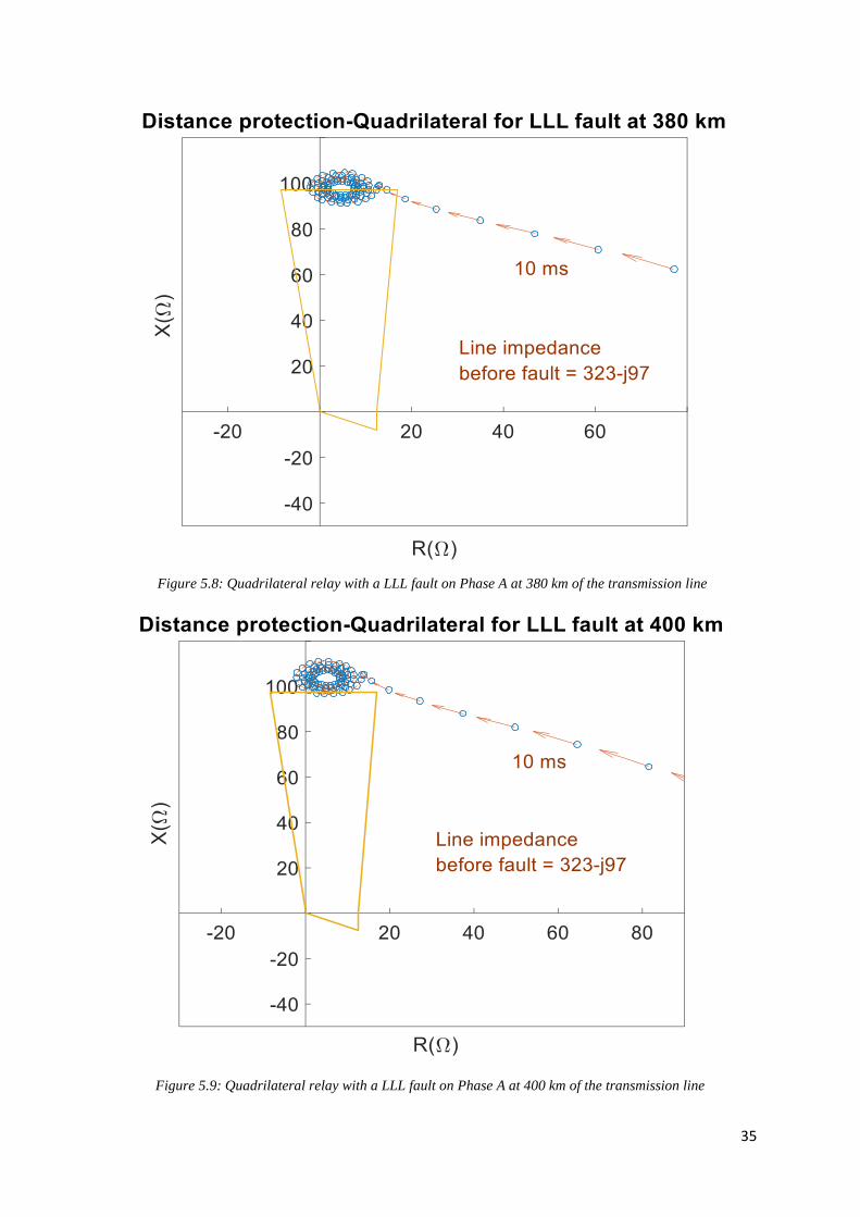
35
Figure 5.8: Quadrilateral relay with a LLL fault on Phase A at 380 km of the transmission line
Figure 5.9: Quadrilateral relay with a LLL fault on Phase A at 400 km of the transmission line
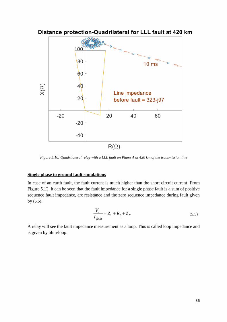
36
Figure 5.10: Quadrilateral relay with a LLL fault on Phase A at 420 km of the transmission line
Single phase to ground fault simulations
In case of an earth fault, the fault current is much higher than the short circuit current. From
Figure 5.12, it can be seen that the fault impedance for a single phase fault is a sum of positive
sequence fault impedance, arc resistance and the zero sequence impedance during fault given
by (5.5).
1a
f N
fault
Z R ZV
I (5.5)
A relay will see the fault impedance measurement as a loop. This is called loop impedance and
is given by ohm/loop.
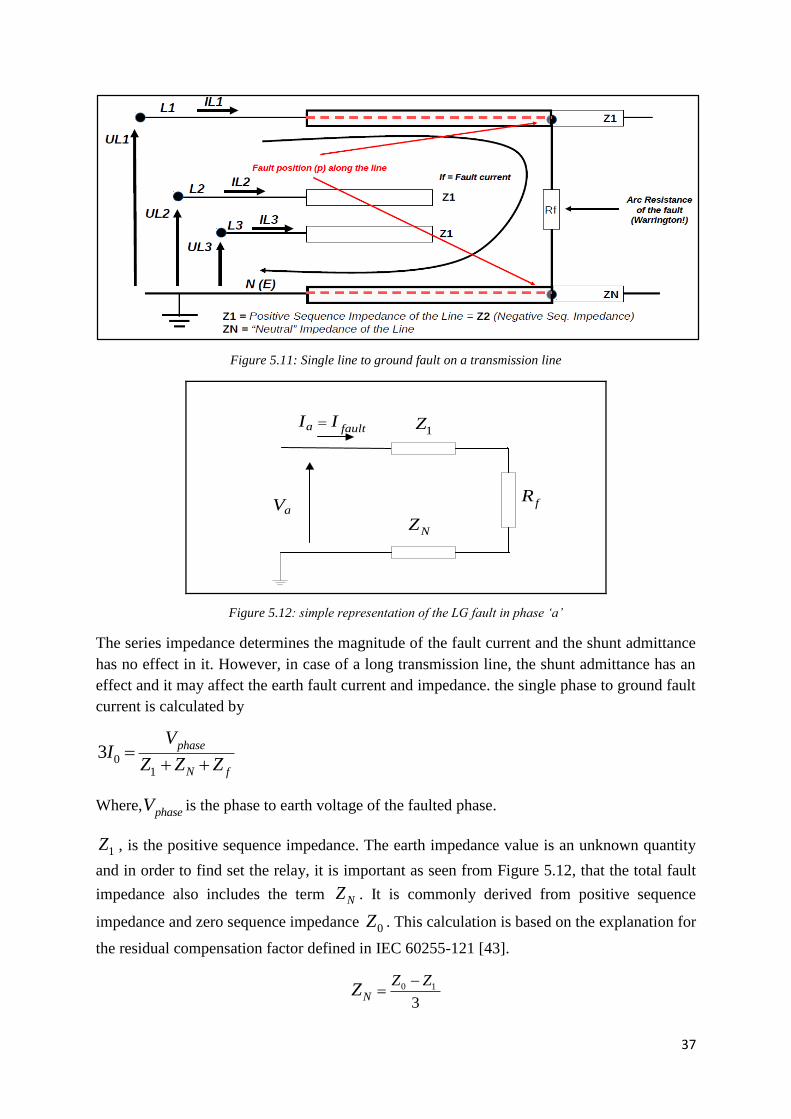
37
Figure 5.11: Single line to ground fault on a transmission line
a faultI I
1Z
NZ
fR
aV
Figure 5.12: simple representation of the LG fault in phase ‘a’
The series impedance determines the magnitude of the fault current and the shunt admittance
has no effect in it. However, in case of a long transmission line, the shunt admittance has an
effect and it may affect the earth fault current and impedance. the single phase to ground fault
current is calculated by
01
3phase
N f
VI
Z Z Z
Where,phaseV is the phase to earth voltage of the faulted phase.
1Z , is the positive sequence impedance. The earth impedance value is an unknown quantity
and in order to find set the relay, it is important as seen from Figure 5.12, that the total fault
impedance also includes the term NZ . It is commonly derived from positive sequence
impedance and zero sequence impedance 0Z . This calculation is based on the explanation for
the residual compensation factor defined in IEC 60255-121 [43].
0 1
3N
Z ZZ
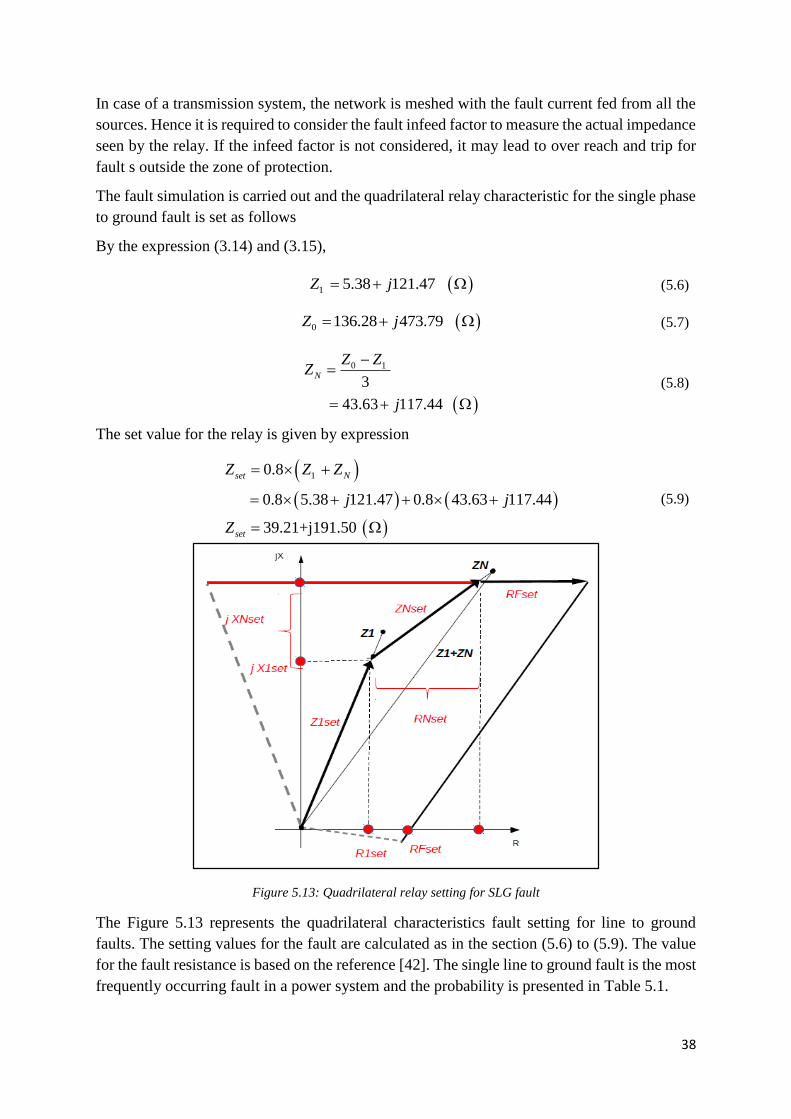
38
In case of a transmission system, the network is meshed with the fault current fed from all the
sources. Hence it is required to consider the fault infeed factor to measure the actual impedance
seen by the relay. If the infeed factor is not considered, it may lead to over reach and trip for
fault s outside the zone of protection.
The fault simulation is carried out and the quadrilateral relay characteristic for the single phase
to ground fault is set as follows
By the expression (3.14) and (3.15),
1 5.38 121.47Z j (5.6)
0 136.28 473.79Z j (5.7)
0 1
3
43.63 117.44
N
Z ZZ
j
(5.8)
The set value for the relay is given by expression
10.8
0.8 5.38 121.47 0.8 43.63 117.44
39.21+j191.50
set N
set
Z Z Z
j j
Z
(5.9)
Figure 5.13: Quadrilateral relay setting for SLG fault
The Figure 5.13 represents the quadrilateral characteristics fault setting for line to ground
faults. The setting values for the fault are calculated as in the section (5.6) to (5.9). The value
for the fault resistance is based on the reference [42]. The single line to ground fault is the most
frequently occurring fault in a power system and the probability is presented in Table 5.1.
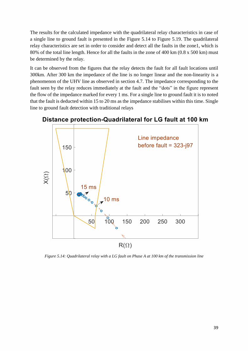
39
The results for the calculated impedance with the quadrilateral relay characteristics in case of
a single line to ground fault is presented in the Figure 5.14 to Figure 5.19. The quadrilateral
relay characteristics are set in order to consider and detect all the faults in the zone1, which is
80% of the total line length. Hence for all the faults in the zone of 400 km (0.8 x 500 km) must
be determined by the relay.
It can be observed from the figures that the relay detects the fault for all fault locations until
300km. After 300 km the impedance of the line is no longer linear and the non-linearity is a
phenomenon of the UHV line as observed in section 4.7. The impedance corresponding to the
fault seen by the relay reduces immediately at the fault and the “dots” in the figure represent
the flow of the impedance marked for every 1 ms. For a single line to ground fault it is to noted
that the fault is deducted within 15 to 20 ms as the impedance stabilises within this time. Single
line to ground fault detection with traditional relays
Figure 5.14: Quadrilateral relay with a LG fault on Phase A at 100 km of the transmission line
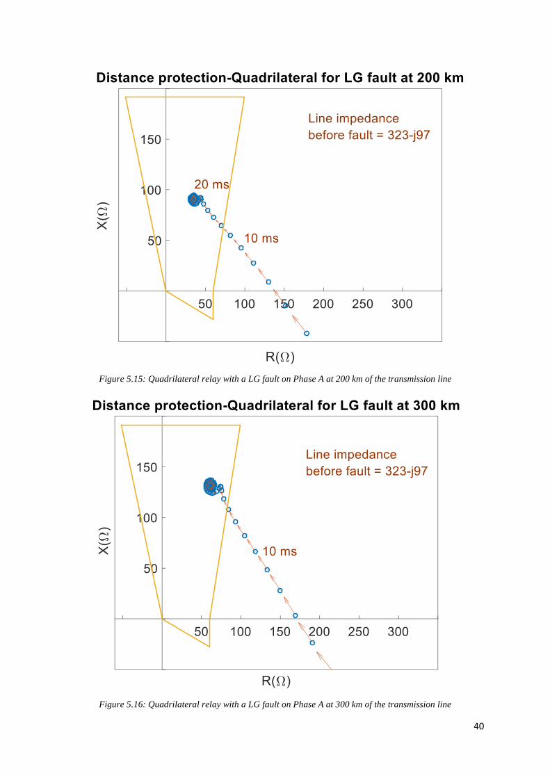
40
Figure 5.15: Quadrilateral relay with a LG fault on Phase A at 200 km of the transmission line
Figure 5.16: Quadrilateral relay with a LG fault on Phase A at 300 km of the transmission line

41
Figure 5.17: Quadrilateral relay with a LG fault on Phase A at 380 km of the transmission line
Figure 5.18: Quadrilateral relay with a LG fault on Phase A at 400 km of the transmission line
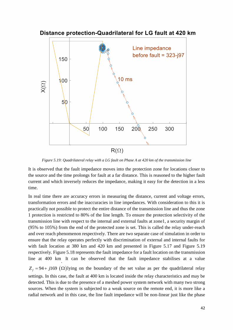
42
Figure 5.19: Quadrilateral relay with a LG fault on Phase A at 420 km of the transmission line
It is observed that the fault impedance moves into the protection zone for locations closer to
the source and the time prolongs for fault at a far distance. This is reasoned to the higher fault
current and which inversely reduces the impedance, making it easy for the detection in a less
time.
In real time there are accuracy errors in measuring the distance, current and voltage errors,
transformation errors and the inaccuracies in line impedances. With consideration to this it is
practically not possible to protect the entire distance of the transmission line and thus the zone
1 protection is restricted to 80% of the line length. To ensure the protection selectivity of the
transmission line with respect to the internal and external faults at zone1, a security margin of
(95% to 105%) from the end of the protected zone is set. This is called the relay under-reach
and over reach phenomenon respectively. There are two separate case of simulation in order to
ensure that the relay operates perfectly with discrimination of external and internal faults for
with fault location at 380 km and 420 km and presented in Figure 5.17 and Figure 5.19
respectively. Figure 5.18 represents the fault impedance for a fault location on the transmission
line
at 400 km. It can be observed that the fault impedance stabilises at a value
94 169fZ j lying on the boundary of the set value as per the quadrilateral relay
settings. In this case, the fault at 400 km is located inside the relay characteristics and may be
detected. This is due to the presence of a meshed power system network with many two strong
sources. When the system is subjected to a weak source on the remote end, it is more like a
radial network and in this case, the line fault impedance will be non-linear just like the phase
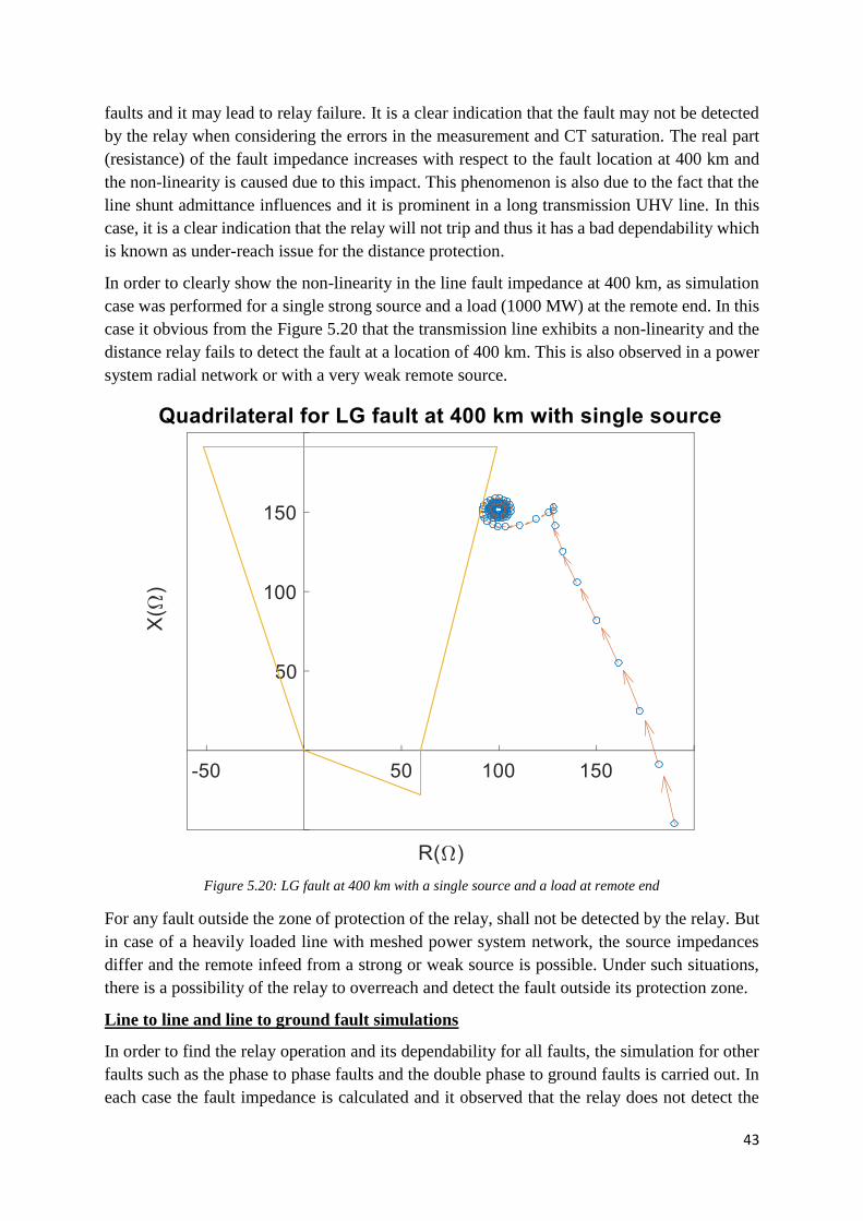
43
faults and it may lead to relay failure. It is a clear indication that the fault may not be detected
by the relay when considering the errors in the measurement and CT saturation. The real part
(resistance) of the fault impedance increases with respect to the fault location at 400 km and
the non-linearity is caused due to this impact. This phenomenon is also due to the fact that the
line shunt admittance influences and it is prominent in a long transmission UHV line. In this
case, it is a clear indication that the relay will not trip and thus it has a bad dependability which
is known as under-reach issue for the distance protection.
In order to clearly show the non-linearity in the line fault impedance at 400 km, as simulation
case was performed for a single strong source and a load (1000 MW) at the remote end. In this
case it obvious from the Figure 5.20 that the transmission line exhibits a non-linearity and the
distance relay fails to detect the fault at a location of 400 km. This is also observed in a power
system radial network or with a very weak remote source.
Figure 5.20: LG fault at 400 km with a single source and a load at remote end
For any fault outside the zone of protection of the relay, shall not be detected by the relay. But
in case of a heavily loaded line with meshed power system network, the source impedances
differ and the remote infeed from a strong or weak source is possible. Under such situations,
there is a possibility of the relay to overreach and detect the fault outside its protection zone.
Line to line and line to ground fault simulations
In order to find the relay operation and its dependability for all faults, the simulation for other
faults such as the phase to phase faults and the double phase to ground faults is carried out. In
each case the fault impedance is calculated and it observed that the relay does not detect the
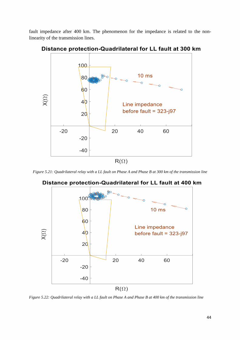
44
fault impedance after 400 km. The phenomenon for the impedance is related to the non-
linearity of the transmission lines.
Figure 5.21: Quadrilateral relay with a LL fault on Phase A and Phase B at 300 km of the transmission line
Figure 5.22: Quadrilateral relay with a LL fault on Phase A and Phase B at 400 km of the transmission line
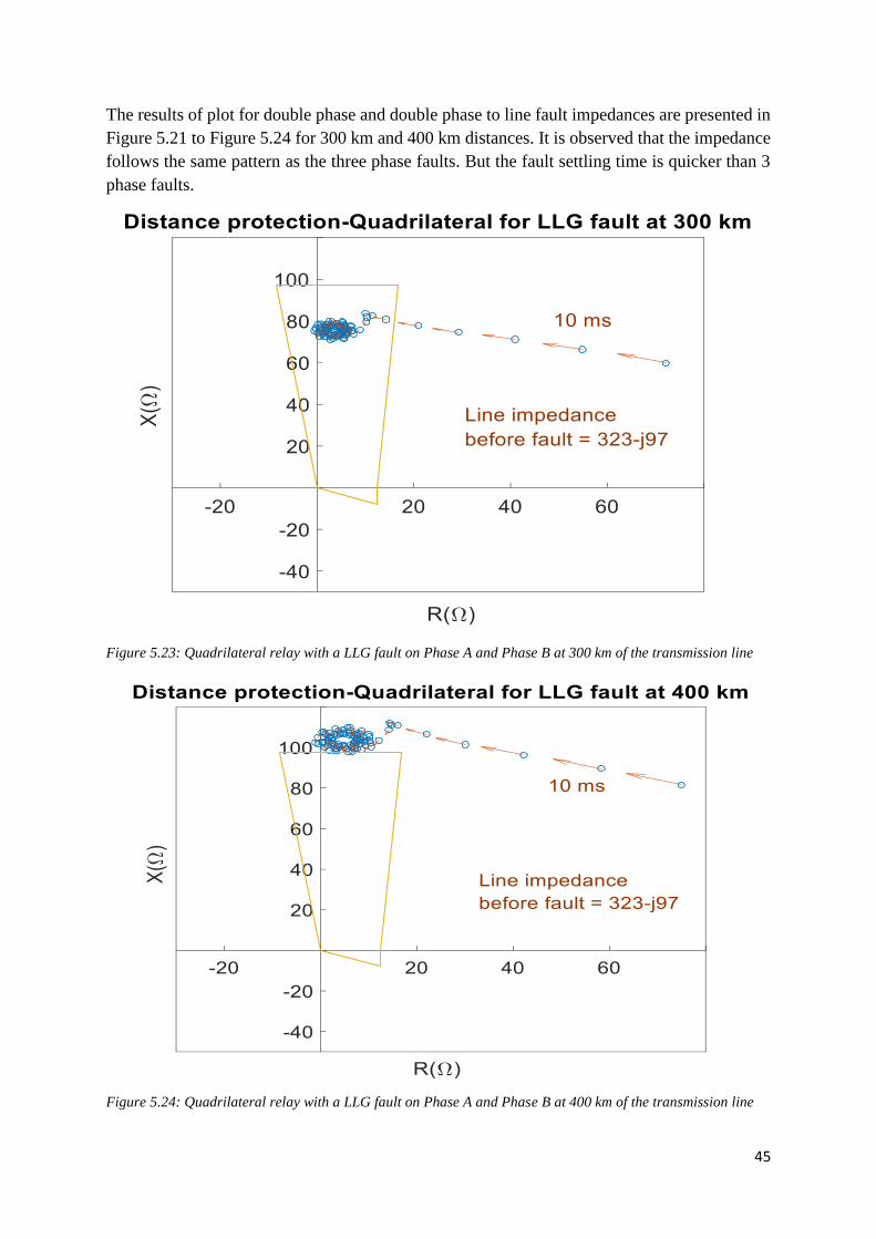
45
The results of plot for double phase and double phase to line fault impedances are presented in
Figure 5.21 to Figure 5.24 for 300 km and 400 km distances. It is observed that the impedance
follows the same pattern as the three phase faults. But the fault settling time is quicker than 3
phase faults.
Figure 5.23: Quadrilateral relay with a LLG fault on Phase A and Phase B at 300 km of the transmission line
Figure 5.24: Quadrilateral relay with a LLG fault on Phase A and Phase B at 400 km of the transmission line
46
Chapter 6
Conclusions and future work
6 CLOSURE
6.1 CONCLUSIONS
From the analysis of the UHV transmission system with a 765 kV transmission line model, the
following conclusions can be drawn
The UHV transmission system in a complex meshed power system is more
advantageous in transferring maximum power with lesser losses and least right of way.
UHV transmission line exhibit certain characteristics such as the dc decay time constant
effect, high capacitive line charging currents and non-linearity of the measured fault
impedance. In case of dc decay, owing to the less resistance compared to the reactance,
the decaying component of the fault transients have a larger value of time constant
(X/R). The value of time constant and the short circuit capacity is important in
protection system design with respect to the minimum delay for the circuit breaker
tripping. The larger time constant of UHV transmission lines requires more time delay
in conventional phasor based protection systems in comparison with a low voltage
transmission system (e.g., 230 kV, 400 kV)
Another interesting phenomenon of the UHV line is related to the capacitor line
charging currents which accounts to almost 50% of the load current. In order to avoid
the effect of the line capacitances, shunt reactors compensation is provided at both the
sending and receiving end of the UHV transmission system. A shunt reactor
compensation will also reduce the higher voltage levels due to the presence of line
capacitances.
A UHV line modelled with distributed line parameters provides results of transient
phenomenon close to the practical scenario, when compared to a lumped line model.
With respect to the distributed line parameter model, it is observed that the fault
impedance measured along a UHV transmission corresponding to various fault
locations is not linear in comparison with a lumped line model. The non-linearity of the
fault impedance measured for all types of shunt fault are presented in the report and the
effect is prominent as the fault location on the line increases. Since the UHV
transmission systems are utilised for long distance power integration, the non-linearity
is more evident in such cases and it pose a challenge to conventional protection systems.
The system subjected to various fault transients and the measured impedance for
different locations of the faults is plotted with traditional quadrilateral relay
characteristics. It was observed that the fault detection is not effective at a fault location
of 80% of the line length. This phenomenon was observed for all the types of faults. It
is noticed that the traditional relay characteristics are based on the lumped line model
of the transmission line and it is no longer accurate for a UHV transmission line. The
effect may lead to a relay failure with bad dependability. This is called an under reach
issue in power system protection. Thus it can be said that the traditional relay model
47
with lumped line parameters is not accurate and the relay algorithm needs to be
modified to account for the changes in the UHV transmission system.
It is also observed form the analysis that the fault impedance values stabilize inside the
relay zone after a certain time generally accounting in the range of 15 to 20 ms. This is
the minimum time required for the fault impedance to be measured in order to issue a
trip signal for the circuit breakers. As the fault location increases, the time for
stabilizing the impedance may also increase.
6.2 FUTURE WORK
The work presented in this thesis report is based on the UHV transmission line model which is
in line with the practical UHV line parameters based on collected inputs. With the simulation
and the analysis for the challenges in UHV transmission system, it is verified that the fault
impedance of the line is non-linear.
The traditional distance relays based on the lumped line parameters are not suited for the UHV
transmission lines of very long distances. This study is carried out for a 765 kV line condition.
According to the market survey scenario, it is observed that the transmission voltage level (>
1000 kV) has been further increased with very long distance of bulk power transmission in
some practical applications. In such a case the non-linearity is even more prominent and the
relay is less dependable.
Further research is recommended in modifying the existing relay algorithm based on non-linear
model to suit for a practical UHV transmission system over long distances with higher
transmission capacity.
48
Bibliography
[1] B. Lundqvist, “100 years of relay protection, the Swedish ABB relay history.”
[2] W. Yi-qiong, C. Hai-yan, L. Bao-jin, and F. Jing, “Design and research of UHV AC
substation,” Eur. Trans. Electr. Power, vol. 22, no. 1, pp. 17–32, 2012.
[3] SIEMENS AG Energy Sector, “High-Voltage Circuit-Breakers: Trends and Recent
Developments,” 2014.
[4] B. Wang, S. Wang, Y. Xiong, X. Wang, L. Tang, and Z. Zuo, “The Development of the
UHV AC Arresters,” Eur. Trans. Electr. Power, vol. 22, no. 1, pp. 94–107, 2012.
[5] G. Gela, “UHV Transmission lines worldwide,” 2015.
[6] U. S. Department of Energy, “Electrical and Mechanical Design Criteria : or EHV and
UHV herhead Transmission Lines,” 1980.
[7] M. Z. Habib, “The Impact if UHV AC transmission line characteristics in traditional line
differential protection.” .
[8] M. Whelan, J. Cunningham, and S. Rockwell, “AC Power History and Timeline.”
[Online]. Available: http://www.edisontechcenter.org/AC-PowerHistory.html. [Accessed:
10-Feb-2016].
[9] Z. Liu, “Grid Development and Voltage Upgrade,” Academic Press, 2014, pp. 4–7.
[10] R. Lings, V. Chartier, and P. S. Maruvada, “Overview of transmission lines above 700
kV,” in Proceedings of the Inaugural IEEE PES 2005 Conference and Exposition in
Africa, 2005, pp. 33–43.
[11] M. Candas and O. S. Meric, “The Application of Ultra High Voltage in the World,” J.
Power Energy Eng., vol. 3, no. 3, pp. 453–457, 1960.
[12] D. Huang, Y. Shu, J. Ruan, and Y. Hu, “Ultra High Voltage Transmission in China:
Developments, Current Status and Future Prospects,” Proc. IEEE, vol. 97, no. 3, pp. 555–
583, Mar. 2009.
[13] N. Hylten-Cavallius and D. Train, “The IREQ Ultra High Voltage Laboratory and
Test Facilities,” IEEE Trans. Power Appar. Syst., vol. PAS-93, no. 1, pp. 176–186, Jan.
1974.
[14] Y. Yamagata, M. Ono, K. Sasamori, and K. Uehara, “Important technologies applied
for UHV AC substations in Japan,” Eur. Trans. Electr. Power, vol. 22, no. 1, pp. 33–48,
Jan. 2012.
[15] Pioneer Transmission, “Advantages of 765 kV Technology.” [Online]. Available:
http://www.pnrtransmission.com/about/docs/Advantages-of-765kV.pdf. [Accessed: 08-
Mar-2016].
[16] Electric Transmission America, “Looking Towards the Future : Advantages of 765-
kV Transmission Technology.”
[17] X. Hu, M. Thomas, and L. Zhang, “TLG on China : UHV Slow progress but
momentum is building,” The Lantau Group (HK) Ltd., no. 38, pp. 1–11, 2014.
[18] Eskom Transmission Division, “Transmission Development Plan (2004 - 2013),”
2013.
[19] Power Grid Corporation of India Ltd., “Transmission and Distribution in India.”
[20] H. Huang, V. Ramaswami, and D. Retzmann, “UHV 1200 kV AC Transmission,”
2007.
[21] American Electric Power, “AEP Transmission Facts,” 2008.
[22] ITAPU Binaconial, “Integration with the Brazilian system.” [Online]. Available:
https://www.itaipu.gov.br/en/energy/integration-brazilian-system. [Accessed: 12-Mar-
2016].
49
[23] INMR, “Project Highlighted Evolution of 765 kV Line Design at American Utility.”
[Online]. Available: http://www.inmr.com/project-highlighted-evolution-765-line-design-
at-american-utility/. [Accessed: 12-Mar-2016].
[24] “Electric power transmission in Venezuela.” [Online]. Available:
http://www.skyscrapercity.com/showthread.php?t=1888596. [Accessed: 12-Mar-2016].
[25] “Update on South Africa transmission projects | ESI-Africa.com.” [Online].
Available: http://www.esi-africa.com/news/update-on-south-africa-transmission-
projects/. [Accessed: 15-Mar-2016].
[26] C. Alamo and J. Pardinas, “Georeferential Video for Located Access Road and
Stringing Tension Equipment Places to Install 1366 km OPGW Cables in Existing
Transmission Lines,” in 2006 IEEE/PES Transmission & Distribution Conference and
Exposition: Latin America, 2006, pp. 1–4.
[27] J. D. Jeong Doo Kim, D. Il Dong Il Lee, K. Y. Koo Yong Shin, K. H. Kwang Ho
Yang, H. S. Hee Sung Ahan, and J. Y. Ja Yoon Koo, “KEPCO 765 kV transmission
system development: corona and electric field effects studies,” in Proceedings 1995
International Conference on Energy Management and Power Delivery EMPD ’95, 1995,
vol. 1, pp. 288–291.
[28] “Voltagewise ckm & MVA declared under commercial operation till 30.04.16 in
different Regions of POWERGRID.”
[29] F. C. E. S. A, “Furnas Centrais Elétricas S.A.,” no. Dc, 2013.
[30] I. chida, Y. Ozaki, and Y. Sekine, “Latest developments in the Japanese 1000 kV
transmission technology,” CIGRE, pp. Session Rep., 1988, 28–04.
[31] Z. Y. Liu, Ultra-HighVoltage Grid. Beijing, China, 2005.
[32] “The Testing Model of China 1000 kV Transmission Power System,” CEPRI.
[33] J. Marti, “Accurate Modellling of Frequency dependent transmission lines in
electromagnetic transient simulations,” in IEEE transactions on power apparatus and
systems, p. PAS–101,pp. 147–155.
[34] “Electrical and Mechanical design criteria for EHV and UHV Overhead Transmission
lines.” US Deperatment of Energy, Jun-1980.
[35] D.-I. Lee and O. Chang-Hyo, “Korea’s First 765-kV Double-Circuit Line,” T&D
World Magazine, 01-Jun-2006.
[36] A. Francisco de Miranda, “Sural Product Catalog-ACSR.” SURAL.
[37] P. Kundur, Power System Stability and Control. McGraw-Hill, Inc.
[38] Y. Xue, D. Finney, and B. Le, “Charging Current in Long Lines and High-Voltage
Cables – Protection Application Considerations,” 2013.
[39] R. B. Laughlin and S. Mukhopadhyay, “STANDARD PARAMETER OF 800 KV
CLASS TRANSMIISSION SYSTEM IN INDIA.”
[40] Y. . Paithankar and S. . Bhide, Fundamentals of Power System Protection, Second
Edition. PHI Learning Private Ltd, 2014.
[41] “Line distance protection REL670 Application Manual.” ABB AB, Substation
Automation Products, Feb-2015.
[42] V. De Andrade, “Typical expected values of the fault resistance in power systems,” in
2010 IEEE/PES, 2010.
[43] “IEC 60255-121:2014 Measuring relays and protection equipment-Part121:
Functional requirements fro distance protection.” IEC, 2014.

TRITA -EE 2016:153
ISSN 1653-5146
www.kth.se