The Impact of Thin-Capitalization and Earnings Stripping ... ANNUAL MEETINGS/2015-… · The Impact...

The Impact of Thin-Capitalization andEarnings Stripping Rules in the EU-15 on theTax ShieldCarmen Bachmann*

University of LeipzigInstitute for Accounting, Finance and TaxationGrimmaische Strasse 12, 04109 Leipzig, GermanyTel: +49 341 9733-591, Fax: +49 341 9733-599

E-mail: [email protected]

Alexander LahmannHHL Graduate School of ManagementJunior Professorship for M&A in SMEJahnallee 59, 04109 Leipzig, GermanyTel: +49 341 9851-665, Fax: +49 341 9851-689

E-mail: [email protected]

Carolin SchulerUniversity of LeipzigInstitute for Accounting, Finance and TaxationGrimmaische Strasse 12, 04109 Leipzig, GermanyTel: +49 341 9733-590, Fax: +49 341 9733-599E-mail: [email protected]

Abstract

Several countries within the EU-15 group limit the tax deductibility of interest payments for intragroupfinancing by thin-capitalization rules or following a recent trend by earnings stripping rules that limitthe deductibility on a broader basis. This paper aims at deriving a tax shield valuation framework con-sidering a possible limitation of the tax deductibility of interest imposed by the tax code. We comparethe obtained pricing equations and their impact on the tax shield value. Finally, we show that the inclu-sion of interest limitation rules imply a remarkable reduction of the tax shield value especially for highlyindebted companies.

Keywords: Tax shield, Firm valuation, Thin-capitalization rules, Earnings stripping rulesJEL classification: G12, G31, G32, K34

*Corresponding author. University of Leipzig, Institute for Accounting, Finance and Taxation,Grimmaische Strasse 12, 04109 Leipzig, Germany, E-mail: [email protected]

1. Introduction

Since the financial crisis in 2008 / 2009 politicians and the general public discuss limiting the taxdeductibility of interest payments in order to render less attractive excessive debt financing. In 2010 thePresident’s Economic Advisory Board stated in their report on tax reform options ‘(...) a limitation on thenet interest deductibility would lessen the bias against equity financing (...), thereby reducing the leverageof firms and the likelihood of future financial distress.’ In Europe similar statements have been made: ‘thecrisis is most definitely the result of excessive debt (...)’(see Rasmussen (February 2009)). This kind oftopic is not new. Already in the early 1990s several governments introduced or at least discussed thelimitation of the tax deductibility of interest expenses by thin-capitalization rules.

Among the first, in 2008, the German government limited the tax deductibility of interest paymentsby introducing an earnings stripping rule, followed by several other EU countries. In contrast to thethin-capitalization rules, these earnings stripping rules are significantly more comprehensive in terms oftheir applicability. The thin-capitalization rules usually limit the intragroup tax deductibility of interestpayments made by foreign subsidiaries and therefore these rules are restricted to a very small field ofapplication. As a response to a decision by the European Court of Justice (ECJ) in 2002, many EUcountries extended their rules to domestic intragroup interest payments. As depicted in Table 1, in themeantime several EU-15 countries dismissed their old thin-capitalization rules for adopting an earningsstripping / interest deductibility rule.1 These rules control the tax deductibility of interest expenses foralmost all types of firms and debt.

Table 1Timeline of Thin-Capitalization and Earnings Stripping Rules in the EU-15

This table shows for countries within the EU-15 group the timeline whether thin-capitalization or earnings strippingrules are applicable. It starts with the year 2004 as the ECJ decision with respect to the then prevailing thin-capitalization rules became effective on January 1, 2004. For example in the case of Denmark (DEN), the tableshows that from 2004 until 2007 a thin-capitalization rule was applicable and since 2008 by an earnings stripping rule.

Earnings stripping / interest deductibility rule GER, DEN, ITA ESP FRA, NED1,POR FIN, GRE

Thin-capitalization rule for all shareholdersBEL, DEN2, FRA, GER, ITA, NED, UK3 FRA4 GRE

Thin-capitalization rule for foreign shareholdersPOR, ESP4 POR5

2004 2007 2008 2009 2010 2012 2013 2014

1 Interest deductibility rule.2 Supplemented by an ‘interest ceiling rule’ in 2008.3 With the Finance Act 2004 (July 22, 2004) abolition of a thin-capitalization rule, since 2010 worldwide debt cap (WWDC).4 Introduction of complex thin-capitalization rule.5 Indicating thin-capitalization rule for non-EU shareholders.

Several empirical studies (see, among others, Weichenrieder and Windschbauer (2008), Overeschand Wamser (2010), or Buettner et al. (2012)) confirm that the tax planning behaviour with respect tointercompany debt is influenced by regulations limiting the tax deductibility of interest payments. Studiesregarding the earnings stripping rule (see, for example, Knauer and Sommer (2012)) indicate that theserules reduce tax savings due to debt financing. Therefore it is surprising that there is still a lack of modelsconsidering these tax regulations for pricing the net benefits of interest payments on debt. The foundationfor the standard pricing techniques goes back to the seminal papers of Modigliani and Miller (1958)and (1963) and was further specified by Myers (1974) who introduced the adjusted present value (APV)method.

1In the following the term earnings stripping rule is used.

2

The main portion of this literature intensively discusses the proper discounting of the tax savings withrespect to the standard financing policies proposed by Modigliani and Miller as well as Miles and Ezzell(1980) and (1985) (see for the extensive discussion, for example, Fernandez (2004), Fieten et al. (2005),Arzac and Glosten (2005), Cooper and Nyborg (2006) and recently Massari et al. (2007) and Dempsey(2013)). Since the tax shield accounts for a major part of the overall firm value (see, e.g., Graham (2000)),it is important to analyze the influencing parameters. Recently some important articles started discussingthe decreasing effect of default on the tax shield value (see, for example, Cooper and Nyborg (2008),Molnár and Nyborg (2013) or Couch et al. (2012)). Even though the aforementioned is important andthe results obtained are beyond questioning, only few articles started considering the tax regulations thatlimit by law the tax deductibility of interest payments (see, e.g., Knauer et al. (2014)). Obviously, the taxlimitations already have an effect on the tax savings before default occurs. Since a correct pricing of thetax savings is vital for practical valuation settings and has to serve as yardstick for empirical studies, it isimportant to adjust the standard tax shield pricing methods accordingly.

This paper aims at deriving a tax shield valuation framework that is able to determine the effects ofthin-capitalization and the recently introduced earnings stripping rules in the EU-152 countries. Hence wecan demonstrate the impact on the enterprise value and on the decision between debt and equity financing.Further we provide an overview on the respective tax regulations in the EU-15 countries. Over and abovewe allow for personal taxes in our framework, as they have a strong impact on the tax advantage of debt(see, e.g., Miller (1977)).

The paper proceeds as follows. Section 2 describes the APV approach as model framework anda binomial lattice modelling the evolvement of the firm’s free cash flows. Section 3 and 4 derive therespective tax shield pricing models considering the cases of thin-capitalization and earnings strippingrules. Section 5 presents numerical examples that are used for comparing the impact of the differenttax rules on the tax shield value and Section 6 concludes. The derivation of the tax shields and furtherdemonstrations are given in the ‘Appendix’.

2. The general Model Setting

2.1. Standard tax shield valuation

Let us consider the probability space (Ω,F ,P) and the time interval [t,T ], where T → ∞ is possible.The time interval can be partitioned in N periods of equal length ∆t = T−t

N , where an arbitrary subsequentperiod t+1 is defined by t+1 = t+∆t. The market is assumed to be free of arbitrage and the existence of a- to the subjective probability measure P equivalent - risk-neutral probability measure Q is presupposed.Throughout our model analysis we consider a levered firm whose operating assets generate in everyfuture period s, with s > t, an uncertain (unlevered) free cash flow stream FCFU . The free cash flowsare assumed to evolve according to a simple recombining binomial lattice. Consequently, the unleveredfree cash flows increase between two arbitrary periods t and t + 1 by the factor u with a probability p ordecrease by the factor d with probability 1 − p:

FCFUt+1 =

u · FCFU

t , up-movement,d · FCFU

t , down-movement. (1)

An important feature of this recombining binomial lattice is that moving first up and then down orfirst down and then up results in the same state dependent value FCFU

t · u · d = FCFUt · u ·

1u .

2We concentrate on this specific countries as they had already been EU member states in 2004 and therefore enables comparisonbetween thin-capitalization and earnings stripping rules.

3

The standard approach for valuing tax shields by using the APV approach (see for example Myers(1974) or Modigliani and Miller (1958)) presumes that a levered firm with value VL

t performs a financingpolicy with certain (non-stochastic) debt levels Ds in every arbitrary period s, with s ≥ t. We will definethis policy as autonomous financing. In order to account for tax savings due to the tax deductibility ofinterest payments on debt the levered firm value conditional on the available information in period t isdetermined by adding on top of the value of an otherwise identical but unlevered firm the present valueof the future period-specific tax savings TS t according to

VLt =

T∑s=t+1

Et

[FCFU

s

](1 + rU)s−t +

T∑s=t+1

Et

[TS s

](1 + rD)s−t (2)

or in a more explicit form by solely considering corporate taxes τC

VLt = VU

t +

T∑s=t+1

Et

[τC · rD · Ds−1

](1 + rD)s−t , (3)

where VUt denotes the unlevered firm value, rU the cost of equity of an unlevered firm, rD the cost of

debt and Et[.] the expected value operator under the subjective probability measure P conditional onthe available information in period t. For simplicity purposes we assume that the corporate tax rate τC ,the unlevered cost of equity rU and the cost of debt rD are constant. Under the risk-neutral probabilitymeasure Q the levered firm value can be equivalently determined via

VLt =

T∑s=t+1

EQt

[FCFU

s

](1 + r f )s−t +

T∑s=t+1

EQt

[TS s

](1 + r f )s−t , (4)

where EQt [.] is the expectation operator under the risk-neutral probability measure Q conditional on the

available information in t and r f denotes the constant risk-free rate. Note that in this case by only consid-ering corporate taxes τC the period-specific tax savings TS s can be explicitly expressed by τC · r f · Ds−1.Assuming a perpetual debt level, i.e. debt stays constant Dt = Dt+1 = ... = DT , we get the classic resultthat the present value of the tax savings simplifies to τC ·rD·Dt

rD= τC · Dt.

By considering personal taxes on payments to equity holders as dividends which are taxed on thepersonal level with a tax rate τP, the tax shield increases to

[τC + (1 − τC) · τP

]· rD · Dt. While interest

payments on a corporate level reduce corporate and personal taxes, the interest income is taxed at thepersonal level with a tax rate τD, which in turn decreases the tax savings to

[τC + (1−τC) ·τP−τD

]·rD ·Dt.

In an extreme scenario, the taxation of interest income on a personal level could exceed the tax advantageof debt. Therefore the marginal benefit of one unit interest payment instead of one equity payout amountsto

(1 − τD) − (1 − τC) · (1 − τP). (5)

This implies that the levered firm value considering personal taxes on dividends τP and interest paymentsτD as well as the after-tax cost of debt rD · (1 − τD) for discounting the future tax savings is determinedby (see for example Miller (1977), Graham (2003) or van Binsbergen et al. (2010))

VLt = VU

t +

T∑s=t+1

Et

[[(1 − τD) − (1 − τC) · (1 − τP)

]· rD · Ds−1

][1 + rD · (1 − τD)

]s−t . (6)

4

This pricing equation can be easily transferred into a model utilizing the risk-neutral probability measure.

2.2. Modelling intercompany financingThe standard approach for valuing tax shields determines the tax shield on a single firm basis. In order

to be able to analyze the impact of a thin-capitalization rule and for highlighting the differences to anearnings stripping rule, we have to extend the single firm framework by considering the interrelations ongroup level, for example the relation between a parent company and an exemplary subsidiary with respectto debt financing. Figure 1 depicts the parent-subsidiary framework for our model analysis. The overalldebt level of the subsidiary amounts in an arbitrary period t to Dsub

t . The subsidiary borrowed a proportionof α, with α ∈ [0, 1], of its total debt from an external debtholder and 1 − α from the subsidiary’s parentcompany. For simplicity purposes we assume that the applicable cost of debt rD are the same for bothdebt issues. Consequently, the total interest payments of the subsidiary amount to I sub

t+1 = rD · Dsubt and by

applying the respective proportions the interest payments distributed to the external debtholders, α · I subt+1 ,

as well as the interest payments for the parent company, (1 − α) · I subt+1 , can be obtained. The subsidiary’s

after-tax income is completely distributed to the parent company and afterwards to the individual investor.In addition, we assume that the parent company has in an arbitrary period t a debt level of Dpar

t and paysinterest payments of Ipar

t+1 = rD · Dpart to external debtholders.

Fig. 1Relationship between Parent and Subsidiary.

This figure depicts the financing relationship between the parent and the subsidiary. The subsidiary finances a proportion α of itsoverall debt Dsub from an external claim holder and (1−α) from its parent company. Accordingly, the interest payments (1−α) · I sub

are paid to the parent and α · I sub to the external claim holder. The parent might finance its operations partly by debt with an amountof Dpar and pays interest Ipar .

For analyzing the overall impact of a thin-capitalization rule on the tax shield value on an individuallevel, we have to assume that the shareholders of the parent company are as well the debtholders underconsideration. In order to avoid an indirect substantial participation of the shareholders in the subsidiary,we additionally assume that the subsidiary is fully owned by the parent and that the number of free floatshares of the parent amounts to 100%.

5

Thin-capitalization and earnings stripping rules target on the limitation of extensive debt financing. A(consistent) model that aims at mapping these tax rules additionally has to deal with thin capitalized, ormore precisely with highly levered firms. Since we model the unlevered free cash flows by a recombiningbinomial tree, the implied equity value in a specific state ω and an arbitrary period t is determined byEt(ω) = VL

t (ω) − Dt might become negative (dependent on the state-dependent free cash flow). Thiswould usually constitute a default due to indebtedness, i.e. Et(ω) < 0. One possibility would be toassume that the firm immediately goes bankrupt. The debtholders could take over the firm and eitherliquidate the remaining assets, sell the overall firm to a new investor or reorganize the firm to carry debtagain. Independent of the new owner of the firm, one of the standard assumptions within this contextis that the tax shield vanishes after default has occurred (see e.g. Cooper and Nyborg (2008) or Koziol(2014)). Another possibility could be to keep the firm running and prevent the default estate by injectingnew equity. In the context of intragroup financing the parent company would inject a new amount ofequity into the subsidiary. The injected amount offsets the negative equity value and up to a lower equitylevel of Ein j

t . We will base our subsequent analysis on the latter assumption and thereby exclude thepossibility of default.

Without any further explanation, the exclusion of default through an equity injection by the parentmight not be reasonable. In general, an equity injection should be modelled depending on its feasibility,i.e. an equity investor would only make an (additional) equity investment if the net present value of theinvestment opportunity would be positive. In case of a negative net present value the equity investorwould not inject new equity and the firm would default. However, in order to perform a selective analysisof the thin-capitalization and earnings stripping rules, the assumption that the parent injects in any casenew equity enables us to independently quantify the effects of these tax regulations on the overall taxshield value.

2.3. Tax shield valuation without interest limitation rules

The classical approach for valuing tax shields builds upon the premise that interest payments are al-ways tax deductible. In order to provide a condensed notation and clear differentiation we use superscriptsdenoting the different cases. In case without any interest limitation rule (N) the overall tax savings withparent-subsidiary financing amount in an arbitrary period t + 1 to

TS Nt+1 =

(Ipart+1 + α · I sub

t+1

)·(1 − τD

)−

(1 − τC

)·(1 − τP

)·[Ipart+1 + (α − y · τC) · I sub

t+1

], (7)

where y denotes the taxable portion of dividend income. Dividend payments distributed from one firm toanother is typically exempted from taxation3 to 95% or 100% or stated differentially a maximum of 5%of the paid dividend is subject to taxes on the parent level.

The tax shield resulting from the parent-subsidiary relation arises due to the following facts: (1.)The subsidiary’s interest expenses result in a decreasing distribution to the parent. This reduces the taxburden by − y · τC . (2.) The tax relief of internal interest expenses at the subsidiary’s level amounting to− τC leads to interest income on the parent level and thereby the tax burden rises by τC . Hence, on theoverall group level the tax shield derives from the double-taxation of dividends. Additionally, note thatthe country specific tax rates (τD, τP and τC) (and below without forestalling, the respective terms for thethin-capitalization rules) have to be plugged-in ex ante to derive the tax shield formula.

3We can consider this, since we assumed that the parent is participated to 100% in the subsidiary. In some countries, e.g. Austria,Belgium, Finland, France, Portugal and most recently Germany (since March 1, 2013), the participation exemption is granted fordividend income with a minimum participation of 10% or 5% (France).

6

3. Thin-Capitalization Rules

3.1. Tax shield valuation with thin-capitalization rulesEven though several approaches (for example Molnár and Nyborg (2013), Couch et al. (2012) or

Koziol (2014)) control for a possible loss of future tax shields due to a possible default, in most taxjurisdictions the tax deductibility of interest payments of the overall firm or group might be limited evenbefore a possible default occurs. Depending on the tax regulation of the jurisdiction either earningsstripping or thin-capitalization rules have been established to limit the tax deductibility of extensive debtfinancing. While the latter have already a long tradition, in several tax codes the earnings stripping rulesare a relatively new trend4 for limiting the tax deductibility of interest payments. Thin-capitalizationrules usually limit to a certain extent the tax deductibility of intragroup interest payments, i.e. interestpayments on debt that has been provided from the parent to a certain subsidiary. In contrast to that,earnings stripping rules are based upon the total interest payments of any company, which implies thatthe interest expenses are limited independent of a parent-subsidiary relation. For explicitly showing theimpact of each of the rules on tax shield valuation, we focus in this section on thin-capitalization rulesand expand our analysis towards earnings stripping rules in section 4.

Throughout our analysis in this section, we will show the impact of the thin-capitalization rules on taxshield valuation that are predominant in the EU-15 countries: Austria (AUT), Belgium (BEL), Denmark(DEN), Finland (FIN), France (FRA), Germany (GER), Greece (GRE), Italy (ITA), Ireland (IRL), Lux-embourg (LUX), Portugal (POR), Spain (ESP), Sweden (SWE) and United Kingdom (UK). As alreadyoutlined in the introduction, we focus on this specific country group due to the impact of the well-knownLankhorst-Hohorst decision5 by the ECJ in 2002 which became effective on January 1, 2004.

As shown in Table 2, the explicit treatment of the non-deductible part of the interest payments impliedby the thin-capitalization rule depends on the country-specific tax code. In some countries the non-tax-deductible internal interest expense is reclassified as dividend paid from the subsidiary to the parent,while in others this is not the case. Due to the fact that on the parent level dividend income is only witha portion of y whereas interest income is entirely subject to taxes, we have to differentiate between thereclassification (rec) and no-reclassification (nor) case.

In the nor-case we observe two effects: (1.) Since a proportion of the overall interest payments is non-deductible for tax purposes, the tax payments increase on the subsidiary’s level and therefore (2.) decreasethe distributions to the parent. Nevertheless, on the parent level these payments are fully taxable sincethese can be regarded as interest income, which in turn implies an overall decrease of the distributions tothe shareholders of the parent. In the rec-case as in the nor-case, the non-tax-deductible interest paymentsimply a higher tax payment by the subsidiary. But in contrast to the nor-case, the reclassification of thenon-tax-deductible part of the internal interest payments implies that the taxes paid by the parent aresmaller as in the nor-case, due to the fact that the reclassified interest income is almost tax exempted.

To determine the excessive internal debt, most countries define a specific debt-to-equity ratio whichwe will denote by DTC

ETC . The interest payments on the debt amount that exceeds DTC

ETC are subject to therespective thin-capitalization rule and therefore not tax-deductible. Since the subsidiary’s considereddebt and equity amount varies across countries between total, only internal, individual internal or internalforeign debt or equity, the applicable debt and equity is determined via h·Dsub

j·E sub .Table 2 provides an overview of the current thin-capitalization rules in the EU-15 countries and

demonstrates the tax shield including thin-capitalization rules. For the analysis of thin-capitalizationrules, we (still) rely on the standard assumptions of the APV approach by assuming that the cost of eq-uity of an unlevered firm rU , the cost of debt rD, the risk free rate r f and the tax rates for personal taxes

4As depicted in Table 1 the German tax legislative was among the first in the EU-15 to implement such a rule. In the USA thepossible introduction of an earnings stripping rule resulted in a broad public discussion.

5ECJ, C-J032/00.

7

Tabl

e2

Cou

ntry

-spe

cific

Thi

n-C

apita

lizat

ion

Rul

esin

the

EU

-15

Cou

ntri

es

Cou

ntry

AUT

BE

LD

EN

2F

IN1

FR

A1

GE

R1

GR

E1

IRL

ITA

1LU

XN

ED

1P

OR

1E

SP1

SWE

UK

Thin

-cap

italiz

atio

nru

leno

yes

yes

noye

sye

sno

noye

sno

yes

yes

yes

noye

s

Kin

dof

shar

ehol

der

all

all

all

all

all

all

non

EU

non

EU

all

Tax

rate

s

Cor

pora

teta

xra

teτ C

25.0

0%33

.99%

24.5

0%20

.00%

36.4

0%30

.18%

26.0

0%12

.50%

27.5

0%29

.22%

25.0

0%31

.50%

30.0

0%22

.00%

21.0

0%

Div

iden

dta

xra

teτP

25.0

0%25

.00%

42.0

0%27

.20%

44.0

0%26

.38%

10.0

0%48

.00%

20.0

0%20

.00%

25.0

0%28

.00%

27.0

0%30

.00%

30.5

6%

Inte

rest

tax

rate

τD

25.0

0%25

.00%

51.5

0%30

.00%

44.0

0%26

.38%

40.9

0%48

.00%

20.0

0%10

.00%

30.0

0%25

.00%

27.0

0%30

.00%

50.0

0%

Subs

tant

ialp

artic

ipat

ion

50.0

0%50

.00%

25.0

0%25

.00%

33.0

0%10

.00%

25.0

0%75

.00%

App

licab

lede

bt-to

-equ

ityra

tioB

=D

TC

ET

C5:

14:

11.

5:1

1.5:

13:

14:

13:

12:

13:

11:

13

Safe

have

nH

t+1

=( 1−α

) ·r D·E

sub

t·

DT

C

ET

C

Tax

shie

ldw

ithth

in-

capi

taliz

atio

n

recl

ass.

asdi

vide

nds

(BE

L,G

ER

,ITA

,ESP

)T

Sre

ct+

1=

( Ipar

t+1

+α·Is

ub t+1) ·( 1

−τD

) −( 1−τ C

) ·( 1−τP) ·[ Ipa

rt+

1+

(1−

y·τ C

)·α·Is

ub t+1−

y·τ C·H

t+1]

nore

clas

s.as

divi

dend

s(D

EN

,F

RA

,N

ED

,P

OR

,U

K)

TS

nor

t+1

=( Ipa

rt+

1+α·Is

ub t+1) ·( 1

−τD

) −( 1−τP) ·[ (1

−τ C

)·Ipa

rt+

1+

[(1−α·τ C

)·(1−

y·τ C

)−(1−α

)·(1−τ C

)]·Is

ub t+1−

(1−

y·τ C

)·τ C·H

t+1]

1E

arni

ngs

stri

ppin

gru

lesi

nce

2008

(GE

R,I

TA),

2012

(ESP

),20

13(F

RA

,NE

D,P

OR

),20

14(F

IN,G

RE

).2

Thi

n-ca

pita

lizat

ion

rule

sap

ply

only

ifan

exem

ptio

nth

resh

old

ofD

KK

10m

illio

nis

exce

eded

.3

Gen

eral

lyac

cept

edar

m’s

-len

gth

prin

cipl

e.

8

Thin-capitalization test in t + 1Application of a thin-capitalization rule (TC):

Parent tax shield without parent-subsidiary financing

TS part+1 =

[(1 − τD) − (1 − τC) · (1 − τP)

]· Ipar

t+1

Interest reclassification (rec)

TS rect+1 =


t+1

)·(1 − τD

)−

(1 − τC

)·(1 − τP

)·[Ipart+1

+ (1 − y · τC) · α · I subt+1 − y · τC · Ht+1

]No interest reclassification (nor)

TS nort+1 =


t+1

)·(1 − τD

)−

(1 − τP

)·[(1 − τC) · Ipar

t+1 + [(1 − α · τC)

·(1 − y · τC) − (1 − α) · (1 − τC)] · I subt+1 − (1 − y · τC) · τC · Ht+1

]

No Application of a thin-capitalization rule (N):

Parent tax shield without parent-subsidiary financing

TS part+1 =

[(1 − τD) − (1 − τC) · (1 − τP)

]· Ipar

t+1

Tax shield with parent-subsidiary financing

TS Nt+1 =


t+1

)·(1 − τD

)−

(1 − τC

)·(1 − τP

)·[Ipart+1 + (α − y · τC) · I sub

t+1

]

Fig. 2Structure of Thin-Capitalization Rules.

This figure shows the tax shield on the level of the individual investor with parent-subsidiary financing, for the cases without andwith the application of a thin-capitalization rule. In the latter we differentiate between the two cases interest reclassification (rec)and no interest reclassification (nor). Note that in the prior period no default has occured.

on interest income τD, dividends τP as well as the corporate income tax τC are constant. In general, acountry-specific thin-capitalization rule can become effective if the current debt-to-equity ratio exceedsDTC

ETC according to Table 2 is applicable.Figure 2 depicts the general setting for the application of an arbitrarily defined thin-capitalization rule.

In the case where it applies (TC), the period-specific tax savings depend on whether the respective taxauthority reclassifies interest paid from the subsidiary to the parent as dividends (rec) or not (nor). Table2 also provides an overview on the country-specific reclassification schemes. However, with respect tothe tax savings in the case where the thin-capitalization rule applies, we may write down for countrieswith interest reclassification

TS rect+1 =


t+1

)·(1 − τD

)−

(1 − τC

)·(1 − τP

)·[Ipart+1 + (1 − y · τC) · α · I sub

t+1 − y · τC · Ht+1

](8)

and for countries without interest reclassification

TS nort+1 =


t+1

)·(1 − τD

)−

(1 − τP

)·[(1 − τC) · Ipar

t+1

+[(1 − α · τC) · (1 − y · τC) − (1 − α) · (1 − τC)

]· I sub

t+1 − (1 − y · τC) · τC · Ht+1

].

(9)

Since we have already differentiated the thin-capitalization rules into a rec- and a nor-case for mappingthe possible interest payments reclassification as dividends, the so called safe haven H remains besidesthe respective tax rate as an important country-specific determinant. It determines the maximum tax-deductible interest payments in an arbitrary period t +1 and is in its most general form in our model given

9

by

Ht+1 = (1 − α) · rD · Dsubt ·

jh·

E subt

Dsubt·

DTC

ETC , (10)

where E subt

Dsubt

represents the inverse debt-to-equity ratio of the subsidiary in an arbitrary period t and DTC

ETC

the ratio DTC

ETC according to the country-specific thin-capitalization rule. By simplifying and noting thatDTC

t =jh · E

subt · DTC

ETC represents the total amount of debt whose interest payments are tax deductible, Ht+1simplifies to

Ht+1 = (1 − α) · rD · DTCt . (11)

As long as the debt-to-equity ratio falls short of DTC

ETC , the interest payments remain fully tax deductible. Ifthe current debt-to-equity ratio exceeds DTC

ETC , equation (11) determines the maximum tax-deductible inter-est payments. Therefore the relation of Dsub

E sub to DTC

ETC determines the calculation of the period-specific taxsavings: Either the tax savings are determined via equation (7) or depending on a possible reclassificationby equation (8) or (9).

With this explicit modelling, it suffices for finding a general expression for the tax shield value todistinguish between a general case representing the application of a thin-capitalization rule TS TC

t+1 and acase without the application TS N

t+1.By following Appendix A we note that TS N

t+1 > TS TCt+1 does not hold for all values of Dsub

t . Thisdirectly implies that the period-specific tax savings in an arbitrary period t are determined by

TS t+1 = min(TS N

t+1, TS TCt+1

)(12)

or equivalently

TS t+1 = TS Nt+1 −max

(TS N

t+1 − TS TCt+1, 0

). (13)

In the following, we derive a model for evaluating the impact of a possible application of a thin-capitalization rule by using a recombining binomial lattice. The implementation is highly interrelatedto the design of the country-specific regulation but can be simplified to a more general form which re-mains applicable by using the specifications of each country according to Table 2.

Under consideration of the risk-neutral probability measure Q, the value of the tax savings in t is inany case given by

VTS t =

T∑s=t+1

EQt

[TS N

s −max(TS N

s − TS TCs , 0

)](1 + r f )s−t . (14)

By the rules of conditional expectations we may write equivalently

VTS t =

T∑s=t+1

EQt

[TS N

s

](1 + r f )s−t︸︷︷︸VTS N

t

−

T∑s=t+1

EQt

[max

(TS N

s − TS TCs , 0

)](1 + r f )s−t . (15)

The first term represents the normal tax shield value according to equation (6) under the risk-neutral

10

probability measure. The second term is an option-like payoff that depends on the specifications of therespective tax code. Regardless of the reclassification treatment, the function TS TC

t+1 depends via theequation for the safe haven on the equity value E sub

t of the levered firm.More explicit versions of the tax shield value equation can be obtained by substituting for TS TC

t+1 therespective equations for the rec- (8) or nor-case (9). In the first one the maximum function in equation (15)is given in an arbitrary period by max

(TS N

t+1 − TS rect+1, 0

). By using equation (7) and (8) and rearranging

we get for the value of the tax shield

VTS rect =

T∑s=t+1

EQt

[TS N

s

](1 + r f )s−t −

T∑s=t+1

(1 − τC

)·(1 − τP

)· y · τC · E

Qt

[max

((1 − α) · I sub

s − Hs, 0)]

(1 + r f )s−t . (16)

The first fraction yields the regular tax shield value without limitation. The second fraction depicts the taxshield reduction caused by a thin-capitalization rule in the rec-case. As non-deductible internal interestexpenses are reclassified as dividends, the term − (1 − τC) · (1 − τP) · y · τC expresses the additionaltaxation on (increased) dividends at the investors level. The term max

((1 − α) · I sub

s − Hs, 0)

representsthe non-deductible part of internal interest expenses which can reach a maximum value of I sub

s for α = 0.In that case no internal interest expenses are tax-deductible since these are reclassified as dividends. Thetax saving, which results from avoiding the double taxation of the subsidiary’s taxable income with τC atthe subsidiary’s and y · τC at the parent company’s level, is eliminated.

By performing an equivalent substitution for the nor-case, we get a slightly different tax shield valua-tion equation

VTS nort =

T∑s=t+1

EQt

[TS N

s

](1 + r f )s−t −

T∑s=t+1

(1 − y · τC

)·(1 − τP

)· τC · E

Qt

[max

((1 − α) · I sub

s − Hs, 0)]

(1 + r f )s−t . (17)

The second fraction represents the tax shield reduction in the nor-case. The term − (1−y ·τC) · (1−τP) ·τC

describes the additional taxes as the internal interest expenses are not deductible at the investors level.When no internal interest expenses are deductible, the tax shield reaches a negative value of − (1 − y) ·(1 − τP) · τC · I sub

s . On the one hand, the tax payments on the subsidiary’s level arise as interest expensesare not deductible (− τC). On the other hand, the taxation of the dividends - which is only taxed by y · τC

- decrease as the distribution to the parent diminishes. The tax shield becomes negative as the interestincome of the parent is still taxed at a rate of τC irrespective of the deduction at the subsidiary’s level.The decreasing distribution to the parent can only slightly cover the negative aspects.

Note that the equations (16) and (17) only differ with respect to the term in front of the maximumfunction. As a direct consequence of the dependency on the safe haven Hs and in turn on the state-dependent equity value of the subsidiary E sub

t , we have to track the equity values for all future states.While this matter can be easily mapped in a binomial lattice, the interdependency of E sub

t in an arbitraryperiod and state from the tax shield value according to Et = VU

t + VTS t − Dt complicates matters (seeFigure 3). We can observe the tax shield depends on the equity value and vice versa. Nevertheless, weovercome this circularity problem by bisection.

11

Initial values:FCFtDt

Valuation formulas:

VUt =

T∑s=t+1

EQt

[FCFU

t+1]

(1 + r f )s−t

VTS t =

T∑s=t+1

EQt

[TS N

s]

(1 + r f )s−t −T∑

s=t+1

EQt

[max(TS N

s − TS recs )

](1 + r f )s−t

VLt = VU

t + VTS t

Et = VLt − Dt

State dependent valuation formulas for the down-state (d):

FCFUt+1(d) = d · FCFU

t

TS Nt+1 = α · rD · Dsub

t ·(1 − τD

)−

(1 − τC

)·(1 − τP

)·[(α − y · τC) · rD · Dsub

t

]max

(TS N

t+1 − TS rect+1, 0

)=(1 − τC

)·(1 − τP

)· y · τC

·max((1 − α) · rD · Dsub

t − (1 − α) · rD · E subt ·

DTC

ETC︸︷︷︸Ht+1

, 0)

State dependent valuation formulas for the up-state (u):

FCFUt+1(u) = u · FCFU

t

TS Nt+1 = α · rD · Dsub

t ·(1 − τD

)−

(1 − τC

)·(1 − τP

)·[(α − y · τC) · rD · Dsub

t

]max

(TS N

t+1 − TS rect+1, 0

)=(1 − τC

)·(1 − τP

)· y · τC

·max((1 − α) · rD · Dsub

t − (1 − α) · rD · E subt ·

DTC

ETC︸︷︷︸Ht+1

, 0)

Fig. 3The Circularity of Thin-Capitalization Rules - A two Binomial Step Example using the Rec-case.

This figure depicts the circularity of the thin-capitalization rule according to the reclassification case (rec) in a two period binomialtree. This tree can easily be adjusted for the nor-case by using the respective equations. For shortening notation we set Ipar

t+1 = 0.With this figure we highlight that the maximum function in both states, up (u) and down (d), in period t + 1 depends on the safehaven Ht+1 and in turn on the equity value in period t. At the same time the equity value is determined via the well-known equationEt = VU

t + VTS t − Dt and therefore, depends on the value of the tax shield. This circularity can be easily overcome by bisection.

3.2. Numerical example: thin-capitalization rules

In this subsection, we show the dynamics of the thin-capitalization rules according to the rec- andthe nor-case in a numerical example by using as basis the aforementioned recombining binomial treefor modelling the evolvement of the unlevered free cash flows. While the recombining feature of theunlevered free cash flows and firm remains intact, the tax shield subject to a possible application of thethin-capitalization rule and in turn the equity value becomes path-dependent. As basis parameters for therecombining binomial lattice we assume an initial free cash flow (FCFU

t ) of 100 an up-factor u = 1.4(d = 1/1.4)6, and equal up- and down-probabilities with q = 0.5. The risk-free interest rate is setaccordingly to 5.714%.

In order to highlight the impact of the thin-capitalization rule on the overall tax shield value, weassume that the parent has no debt outstanding (Dpar = 0) and set α = 0. The subsidiary performs aconstant debt level policy with Dsub = 700 (I sub = 40) which implies a leverage ratio in terms of D/VU inperiod t of 58.33. This debt level has been chosen in order to get as result a clear differentiation betweenstates in which the thin-capitalization rule is not and is applicable. As parameters describing the taxjurisdiction Italy we assume for both cases the following: DTC

ETC = 4, τC = 27.5%, τP = 20%, τD = 20%,j = 1 and h = 1. In case of equity values lower than Et = 10, new equity is injected up to a level ofEin j

t = 10.

6An up-factor of u = 1.4 implies an annual volatility of 33.65% which is an appropriate assumption for the standard deviation ofthe free cash flows of a listed firm in the EU-15.

12

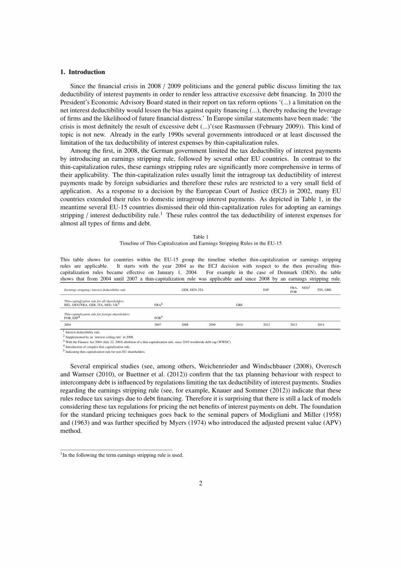
As demonstrated in Figure 4 the present value of the tax shield generated by the subsidiary’s debton the level of the individual investor without considering an application of interest limitation rulesamounts to VTS N

t = 5.583 (in a single period TS Ns = 0.319). By considering the consequences of a

thin-capitalization rule in the rec-case the overall tax shield is given by VTS rect = 5.583 − 0.098 = 5.485.

This small impact of the thin-capitalization rule is subject to the fact that non-deductible interest expensesare reclassified as dividends which are subject to tax. In order to illustrate this, we focus on the uu- andud-state. In the uu-state, the maximum tax-deductible interest amount (10) in our model amounts toHt+2 =

(1 − 0

)·(0.05714 · 700 · 1

1 ·845.583

700 · 41

)= 193.266 (while the complete interest expenses amount

to I subt+2 = 40). The safe haven debt-to-equity ratio is not exceeded 700

845.583 −41 = − 3.172 and all interest

expenses are deductible. As the safe haven exceeds the interest expenses in the specific period, the taxshield for the rec-case TS rec

t+2 =(1 − 0.275

)·(1 − 0.2

)·(0.05 · 0.275 · 193.266

)= 1.541 is higher than the

tax shield without interest limitation. In this case TS Nt+2 < TS rec

t+2 and the function max(TS N

t+2−TS rect+2, 0

)results in max

(0.319 − 1.541, 0

)= 0. The thin-capitalization rule does not apply and the tax shield

value according to equation (13) amounts to TS t+2 = 0.319. In contrast in the dd-state, the safe havendebt-to-equity ratio is exceeded by 700

91.017 −41 = 3.691 and so the safe haven amounts to Ht+2 = 20.804.

As TS rect+2 = 0.166, the maximum function amounts to max

(0.319 − 0.166, 0

)= 0.153 and the final tax

shield is reduced to TS t+2 = 0.319− 0.153 = 0.166. The outstanding interest expenses are not deductibleat the subsidiary’s level and reclassified at the parent level. As the implied equity value gets negative inthe specific case (Et+2 = − 191.954), we assume that it gets injected up to 10.

For the analysis of the nor-case we use the same parameters as aforementioned. As shownin Figure 5 the tax shield considering this respective thin-capitalization rule amounts to VTS nor

t =

5.583 − 3.766 = 1.817. In comparison to the rec-case the non-deductible part of the subsidiary’s in-ternal interest expenses are fully taxable at the parent level resulting in an overall smaller tax shieldvalue. To exemplify with the dd-state the equivalent values amount to Ht+2 = 19.0481, TS nor

t+2 =

−(1 − 0.2

)·[(0.275 − 0.05 · 0.275) · 40 − (1 − 0.05 · 0.275) · 0.275 · 19.048

]= − 0.8 ·

[10.450 −

5.166]

= − 4.227 and max(0.319 − (− 4.227), 0

)= 4.546. In the specific period the tax shield

TS t+2 = 0.319 − 4.546 = − 4.227 gets negative. The tax savings of the deductible interest expenses(− (1−0.2) ·0.05 ·0.275 · (1−0.275) = − 0.152) do not cover the additional taxation of the non-deductibleinterest expenses ((1 − 0.2) · (1 − 0.05) · 0.275 = 4.379)7 anymore.

7See for an explanation Appendix A.

13

FCFUt = 100

VUt = 1200

VTS Nt = 5.583∑

PV(EQt [max(.)]) = 0.098

VL,rect = 1205.485

Et = 505.485

FCFUt+1(d) = 71.429

VUt+1(d) = 785.714∑PV(EQ

t+1[TS Ns ]) = 5.583

max(TS Nt+1 − TS rec

t+1, 0)(d) = 0∑PV(EQ

t+1[max(.)]) = 0.279

VL,rect+1 (d) = 791.017

Et+1(d) = 91.017

FCFUt+2(dd) = 51.020

VUt+2(dd) = 510.204∑PV(EQ

t+2[TS Ns ]) = 5.583


t+2, 0)(dd) = 0.153∑PV(EQ

t+2[max(.)]) = 0.285

VL,rect+2 (dd) = 515.502

Et+2(dd) = 10 (−184.498)

(1−

q)=

0.5

FCFUt+2(du) = 100

VUt+2(du) = 1000∑PV(EQ

t+2[TS Ns ]) = 5.583


t+2, 0)(du) = 0.153∑PV(EQ

t+2[max(.)]) = 0

VL,rect+2 (du) = 1005.583

Et+2(du) = 305.583

q=

0.5

(1−

q)=

0.5

FCFUt+1(u) = 140

VUt+1(u) = 1540∑PV(EQ

t+1[TS Ns ]) = 5.583


t+1, 0)(u) = 0∑PV(EQ

t+1[max(.)]) = 0

VL,rect+1 (u) = 1545.583

Et+1(u) = 845.583

FCFUt+2(ud) = 100

VUt+2(ud) = 1000∑PV(EQ

t+2[TS Ns ]) = 5.583


t+2, 0)(ud) = 0∑PV(EQ

t+2[max(.)]) = 0

VL,rect+2 (ud) = 1005.583

Et+2(ud) = 305.583

(1−

q)=

0.5

FCFUt+2(uu) = 196

VUt+2(uu) = 1960∑PV(EQ

t+2[TS Ns ]) = 5.583


t+2, 0)(uu) = 0∑PV(EQ

t+2[max(.)]) = 0

VL,rect+2 (uu) = 1965.583

Et+2(uu) = 1265.583

q=

0.5

q=

0.5

Fig. 4Numerical Example for a Thin-Capitalization Rule in the Rec-Case.

Throughout this numerical example we use the parameters as given in section 3.2. For providing a clear figure we have abstainedfrom depicting periods with s > t + 2. From period t + 4 onwards we have assumed for ease of calculation a perpetual tax shield of5.583. We denote the different state dependent quantities by the respective up- or down-movements, i.e. the free cash flow in periodt + 2 resulting from one up- and one down-movement is denoted by FCFU

t+2(ud). The results of all calculations are rounded to fourdigits. For completeness and plausibility we show in case of indebtedness the implied negative equity value. Obviously, in case ofa limited liability firm the equity value is then zero; concerning our assumptions it is injected up to 10.

14

FCFt = 100

VUt = 1200

VTS Nt = 5.583∑

PV(EQt [max(.)]) = 3.766

VL,nort = 1201.817

Et = 501.817

FCFUt+1(d) = 71.429

VUt+1(d) = 785.714∑PV(EQ

t+1[TS Ns ]) = 5.583

max(TS Nt+1 − TS nor

t+1, 0)(d) = 0∑PV(EQ

t [max(.)]) = 7.961

VL,nort+1 (d) = 783.335

Et+1(d) = 83.335

FCFUt+2(dd) = 51.020

VUt+2(dd) = 510.204∑PV(EQ

t+2[TS Ns ]) = 5.583


t+2, 0)(dd) = 4.546∑PV(EQ

t+2[max(.)]) = 7.741

VL,nort+2 (dd) = 508.046

Et+2(dd) = 10 (−191.954)

(1−

q)=

0.5

FCFUt+2(du) = 100


t+2[TS Ns ]) = 5.583


t+2, 0)(du) = 4.546∑PV(EQ

t+2[max(.)]) = 0

VL,nort+2 (du) = 1005.583

Et+2(du) = 305.583

q=

0.5

(1−

q)=

0.5

FCFUt+1(u) = 140

VUt+1(u) = 1540∑PV(EQ

t+1[TS Ns ]) = 5.583


t+1, 0)(u) = 0∑PV(EQ

t+1[max(.)]) = 0

VL,nort+1 (u) = 1545.583

Et+1(u) = 845.583

FCFUt+2(ud) = 100


t+2[TS Ns ]) = 5.583


t+2, 0)(ud) = 0∑PV(EQ

t+2[max(.)]) = 0

VL,nort+2 (ud) = 1005.583

Et+2(ud) = 305.583

(1−

q)=

0.5

FCFUt+2(uu) = 196


t+2[TS Ns ]) = 5.583


t+2, 0)(uu) = 0∑PV(EQ

t+2[max(.)]) = 0

VL,nort+2 (uu) = 1965.583

Et+2(uu) = 1265.583

q=

0.5

q=

0.5

Fig. 5Numerical Example for a Thin-Capitalization Rule in the Nor-Case.

Throughout this numerical example we use the parameters as given in section 3.2. For providing a clear figure we have abstainedfrom depicting periods with s > t + 2. From period t + 4 onwards we have assumed for ease of calculation a perpetual tax shieldof 5.583. We denote the different state dependent quantities by the respective up- or down-movements, i.e. the free cash flow inperiod t + 2 resulting from one down- and one up-movement is denoted by FCFU

t+2(du). The results of all calculations are roundedto three digits. For completeness and plausibility we show in case of indebtedness the implied negative equity value. Obviously, incase of a limited liability firm the equity value is then zero; concerning our assumptions it is injected up to 10.

15

Throughout section 5, we show the impact of different debt levels and their implied application of thethin-capitalization rule on the overall tax shield value.

4. Earnings Stripping Rules

4.1. Tax shield valuation with earnings stripping rules

Since 2008, some of the EU-15 countries, i.e. Germany, Italy, Portugal, Spain and in 2014 Finlandand Greece, introduced or replaced their thin-capitalization rules by earnings stripping rules. Accordingto the German model, which can be regarded as a kind of role model8, this limitation applies in general toall interest expenses of a firm, whether the debt is granted by a third party, related party or a shareholder.The deductibility of annual net interest expense rD · Dt

9 (interest expense exceeding interest income)is limited to a certain percentage β of the earnings before interest, tax, depreciation and amortization(EBITDA), if the debt value is above a certain threshold. This debt threshold ranges from 0.5 millionEUR in Finland to 5 million EUR in Greece and is assumed to be exceeded in our framework.

The non-deductible interest expenses ICt+1 can be carried forward and subtracted in future periods.Therefore, there might be a positive influence on the tax shield in future periods as there is a higherdeductible interest potential. In Portugal and Spain the interest carryforward is limited to 5 and 18 years.Without time restriction and disregarding negative EBITDA values it is determined by

ICt+1 = max(rD · Dt + ICt − β · EBIT DAt, 0

). (18)

Thus, the general deductible interest amount is given by

Ψt+1 = min(β · EBIT DAt, rD · Dt + ICt

). (19)

Within the framework of the Growth Acceleration Act (Wachstumsbeschleunigungsgesetz)10, Germanyon the one hand increased the certain threshold from 1 to 3 million EUR and on the other hand introducedthe possibility to carry forward (for 5 years) the amount of the EBITDA which is not used for deductionof interest expenses to cover future excess interest payments. The Spanish and Portuguese legislationsalso allow for a 5-year EBITDA carryforward and Italy for an unlimited one. In the case of an unlimitedEBITDA carryforward, denoted by ECt, the EBITDA carryforward is in an arbitrary period t determinedby

ECt+1 = max(β · EBIT DAt+1 + ECt − rD · Dt − ICt, 0

)(20)

and consequently the tax deductible interest amount is calculated by

Ψt+1 = min(β · EBIT DAt+1 + ECt, rD · Dt + ICt

). (21)

In Germany11 and Finland the earnings stripping rule contains a unique feature referred to as theescape clause which defines the circumstance where the earnings stripping is not applicable. This is thecase when the book-equity-to-total-assets ratio of the financial statement of a group company is minimum

8The discussion of the introduction of an earnings stripping rule in Germany dates back to a resolution of the commission ofimportant key points to the planned german tax reform 2008 on July 2, 2006.

9We assume that the considered firm does not earn any interest income.10Art. 1 of the Growth Acceleration Act, December 22, 2009, BGBl 2009 I, 3950; applicable for fiscal years ending after December

31, 2009.11In Germany a book-equity-to-total-assets ratio of a group company less than 2% of the consolidated one is harmless.

16

as high as the corresponding ratio in the consolidated financial statements of the parent company. Thedifferent structures of the country-specific earnings stripping rules are depicted in Table 3.

In order to compare the effects on the tax shield of thin-capitalization rules and earnings strippingrules, we consider the same framework (parent-subsidiary) for our analysis of the earnings strippingrules12. By following Appendix B, the tax shield under consideration of an earnings stripping rule can bedetermined by

TS ES Rt+1 =


t+1

)·(1 − τD

)−

(1 − τP

)·[Ipart+1 + [(1 − y · τC) − (1 − α) · (1 − τC)] · I sub

t+1

− τC · Ψpart+1 − (1 − y · τC) · τC · Ψ

subt+1

],

(22)

where the tax deductible interest amount Ψ (.)t+1

13 for the parent and the subsidiary is given by

Ψ (.)t+1 = −max

(β · EBIT DA(.)

t+1 + EC(.)t − rD · D

(.)t − IC(.)

t , 0)

+ β · EBIT DA(.)t+1 + EC(.)

t , (23)

the corresponding interest carryforward by

IC(.)t+1 = max

(rD · D

(.)t + IC(.)

t − β · EBIT DA(.)t+1 − EC(.)

t , 0). (24)

For an adequate and detailed analysis of the integrated period specific tax savings given in equation(22), we disentangle this equation into its effect-relationships. The term (1 − τP) · (1 − α) · (1 − τC) ·I subt determines the effect of the internal interest payments on parent-subsidiary debt financing on the

individual level, subject to personal taxes on dividend payments.(Ipart + α · I sub

t

)·(1 − τD

)represents the

effect of interest payments on external debt financing after personal taxes on interest income. In general,the term −

(1 − τP

)·[(τC − y · τC) · I sub

t − (1 − y · τC) · τC · Ψsubt

]maps the combined influence of the

subsidiary’s interest payments originating from internal parent-subsidiary debt financing. In particular,it represents the negative effect as after-tax income on the individual level considering personal taxes ondividend income, i.e. −

(1 − τP

)·(τC − y · τC

)· I sub

t , and the positive effect of the tax deductible interest

payments of the subsidiary subject to the earnings stripping rule, i.e.(1 − τP

)·(1 − y · τC

)· τC · Ψ

subt . It

is important to note that due to a possible application of the earnings stripping rule, Ψ subt might be bigger

than I subt . An equivalent interpretation without the additional taxation on intragroup dividends (y · τC)

paid by the subsidiary to the parent holds for −(1− τP

)·(Ipart − τC · Ψ

part

). The important relation within

the context of the tax deductible interest under the application of an earnings stripping rule is given byequation (23). Independent of the parent or the subsidiary’s level, this equation can be interpreted intwo parts: (1.) A basic and always tax deductible interest amount which is equal to β · EBIT DA(.)

t (pluspossible EC(.)

t ) and (2.) a maximum function which determines the additional tax deductible interest incase the earnings stripping rule does not apply (plus possible IC(.)

t ), i.e. β · EBIT DA(.)t > rD · D

(.)t−1.

In this regard, we would like to turn attention on the difference between the tax benefits due to interestpayments on the corporate level and the tax disadvantage due to interest income on the individual levelin an arbitrary period t, i.e. (τC − τD) · I(.)

t . This difference is positive as long as τC > τD. With anearnings stripping rule due to the limited tax deductibility of interest payments on the corporate levelthis difference is given by τC · Ψ

(.)t+1 − τD · I

(.)t+1. For simplification purposes with ECt = 0, the algebraic

sign of this difference depends on whether the earnings stripping rule applies or not. In case the earningsstripping rule applies, this difference might become negative even for τC > τD due to I(.)

t+1 > Ψ (.)t+1. In

12This is useful, because e.g. in Finland and Greece the non-deductibility criteria applies only for related parties.13Note that we use the general expression (.) within this context as superscript for indicating that the respective formulas are valid

for the parent as well as the subsidiary.

17

Tabl

e3

Cou

ntry

-spe

cific

Ear

ning

sSt

ripp

ing

Rul

esin

the

EU

-15

Cou

ntri

es

Tax

shie

ldw

ithea

rnin

gsst

ripp

ing

rule

sT

SE

SR

t+1

=( Ipa

rt+

1+α·Is

ub t+1) ·( 1

−τD

) −( 1−τP) ·[ Ipa

rt+

1+

[(1−

y·τ C

)−(1−α

)·(1−τ C

)]·Is

ub t+1−τ C·Ψ

par

t+1−

(1−

y·τ C

)·τ C·Ψ

sub

t+1]

Cer

tain

perc

enta

geof

EB

ITD

A( β

)

Exe

mpt

ion

thre

shol

d5

Inte

rest

carr

y-fo

rwar

d

Spar

eE

BIT

DA

carr

yfor

war

dTy

peof

com

pany

Esc

ape

clau

seFo

rmul

afo

rΨ

(.) t+1

Form

ula

for

IC(.) t+

1

FIN

30%

0.5

unlim

ited

-re

late

dpa

rtie

s4ye

sm

in( β·E

BIT

DA

(.) t+1,

r D·D

(.) t+

IC(.) t

)m

ax( r D·D

(.) t+

IC(.) t−β·E

BIT

DA

(.) t+1,

0)

GE

R30

%3

unlim

ited

5ye

ars

allc

ompa

nies

yes

min

( β·E

BIT

DA

(.) t+1

+∑ t−4 n=

tEC

(.) n,t−

∑ t−4 n=tE

C(.) n,

t+1,

r D·D

(.) t+

IC(.) t

)m

ax( r D·D

(.) t+

IC(.) t−β·E

BIT

DA

(.) t+1

−∑ t−4 n=

tEC

(.) n,t,

0)

GR

E60

%1

52un

limite

d-

grou

pm

embe

rs-

min

( β·E

BIT

DA

(.) t+1,

r D·D

(.) t+

IC(.) t

)m

ax( r D·D

(.) t+

IC(.) t−β·E

BIT

DA

(.) t+1,

0)

ITA

30%

-un

limite

dun

limite

d3al

lcom

pani

es4

-m

in( β·E

BIT

DA

(.) t+1

+E

C(.) t,

r D·D

(.) t+

IC(.) t

)m

ax( r D·D

(.) t+

IC(.) t−β·E

BIT

DA

(.) t+1−

EC

(.) t,

0)

PO

R60

%1

35

year

s5

year

sal

lcom

pani

es-

min

( β·E

BIT

DA

(.) t+1

+∑ t−4 n=

tEC

(.) n,t−

∑ t−4 n=tE

C(.) n,

t+1,

r D·D

(.) t+

∑ n−4

n=t

IC(.) n,

t−

∑ t−4 n=tIC

(.) n,t+

1)

ESP

30%

118

year

s5

year

sal

lcom

pani

es-

min

( β·E

BIT

DA

(.) t+1

+∑ t−4 n=

tEC

(.) n,t−

∑ t−4 n=tE

C(.) n,

t+1,

r D·D

(.) t+

∑ t−17

n=t

IC(.) n,

t−

∑ t−17

n=t

IC(.) n,

t+1)

GE

RP

OR

ESP

EC

(.) n,t

=

max

( β·E

BIT

DA

(.) n−

r D·D

(.) s−1,

0) ,fo

rn

=t

max

( ∑ n−4

u=n

EC

(.) u,t−

1−

∑ n−4

u=n−

1E

C(.) u,

t−

max

(rD·D

(.) t−1−β·E

BIT

DA

(.) t,

0),

0) ,fo

rt−

5≤

n≤

t−1

0,fo

rt−

5>

n

ITA

EC

(.) t=

max

( β·E

BIT

DA

(.) t+

EC

(.) t−1−

r D·D

(.) t−1−

IC(.) t−

1,0)

PO

RIC

(.) n,t

=

max

( β·E

BIT

DA

(.) n+

∑ n−5

u=n−

1E

C(.) u,

n−1−

r D·D

(.) t−1,

0) ,fo

rn

=t

max

( ∑ n−4

u=n

IC(.) u,

t−1−

∑ n−4

u=n−

1IC

(.) u,t−

max

(β·E

BIT

DA

(.) t+

∑ t−5 n=t−

1E

C(.) n,

t−1−

r D·D

(.) t−1,

0),

0) ,fo

rt−

5≤

n≤

t−1

0,fo

rt−

5>

n

ESP

IC(.) n,

t=

max

( β·E

BIT

DA

(.) n+

∑ n−5

u=n−

1E

C(.) u,

n−1−

r D·D

(.) t−1,

0) ,fo

rn

=t

max

( ∑ n−17

u=n

IC(.) u,

t−1−

∑ n−17

u=n−

1IC

(.) u,t−

max

(β·E

BIT

DA

(.) t+

∑ t−5 n=t−

1E

C(.) n,

t−1−

r D·D

(.) t−1,

0),

0) ,fo

rt−

5≤

n≤

t−1

0,fo

rt−

5>

n

1In

2014

,red

ucin

gea

chye

arby

10%

until

2017

with

30%

.2

From

2014

-201

5;e

3m

illio

nfr

om20

16.

3E

xces

sin

tere

stex

pens

esof

agr

oup

com

pany

may

beoff

setw

ithsp

are

EB

ITD

Aca

paci

tyof

anot

herg

roup

com

pany

.4

Furt

here

xem

ptio

nsfo

rfina

ncia

l,in

sura

nce

and

pens

ion

inst

itutio

nsan

dpa

rtia

llyfo

rass

ocia

ted

grou

pco

mpa

nies

and

mut

ualr

eale

stat

ean

dho

usin

gco

mpa

nies

.5

Ine

mill

ion.

18

case the earnings stripping rule does not apply, we have two possible scenarios depending on IC(.)t . For

IC(.)t = 0 and I(.)

t+1 = Ψ (.)t+1, the algebraic sign of the difference depends again on the relation of τC and τD.

For a positive IC(.)t we have Ψ (.)

t+1 > I(.)t+1 and the difference might become positive.

With the period specific tax savings subject to a possible application of an earnings stripping rule, thetax shield value under the risk-neutral probability measure Q contingent on the available information in tis determined by

VTS ES Rt =

T∑s=t+1

EQt

[TS ES R

s

](1 + r f )s−t (25)

By substituting the equations (22) and (23) for the parent and the subsidiary into (25) and rearranging weget

VTS ES Rt =

T∑s=t+1

( EQt

[ (I par

s + α · I subs

)·(1 − τD

)−

(1 − τP

)·[I par

s + [(1 − y · τC) − (1 − α) · (1 − τC)] · I subs

]](1 + r f )s−t

+

(1 − τP

)· τC ·

EQ

t

[β · EBIT DApar

s + ECpars−1 −max

(β · EBIT DApar

s + ECpars−1 − I par

s − ICpars−1, 0

)](1 + r f )s−t

+(1 − y · τC

)·

EQt

[β · EBIT DAsub

s + EC subs−1 −max

(β · EBIT DAsub

s + EC subs−1 − I sub

s − IC subs−1, 0

)](1 + r f )s−t

).

(26)

Basically, equation (26) consists of three fractions constituting the tax shield value. We start by discussingthe value increments of the first fraction. The increment

(Ipar

s + α · I subs

)· (1− τD) maps the additional tax

burden on the individual level after taxes on interest income caused by the interest payments of the overallgroup. With α = 0, i.e. the subsidiary is fully financed by parent-subsidiary financing, this term onlyrepresents the additional tax burden caused by debt financing of the parent.

(1−τP

)·(1−α

)·(1−τC

)· I sub

sdetermines the effect of tax payments on dividends of increased dividends payments by the parent tothe individual investors which originate from interests paid by the subsidiary to the parent. The term−

(1 − τP

)·[Ipar

s + (1 − y · τC) · I subs

]represents the combined effect of smaller tax payments on dividends

on the individual level due to the fact that interest payments reduce dividend payments. The second andthird fraction represent the value of the tax deductible interest payments for the parent and the subsidiaryafter personal taxes on dividend payments. In any case, whether the earnings stripping rule applies or not,the added fractions determine the present value of all future tax savings β ·EBIT DAs and possible ECs−1,∀s > t, for the overall group.

19

4.2. Numerical example: earnings stripping rules

In this subsection, we outline a numerical example for an exemplifying earnings stripping rule. Inorder to compare the influence of different interest limitation rules, we rewrite equation (26) by

VTS ES Rt =

T∑s=t+1

EQt

[TS N

s

](1 + r f )s−t −

T∑s=t+1

EQt

[TS N

s − TS ES Rs

](1 + r f )s−t

=

T∑s=t+1

EQt

[TS N

s

](1 + r f )s−t −

T∑s=t+1

EQt

[(1 − τP

)· τC ·

[Ipar

s − Ψpars + (1 − y · τC) · (I sub

s − Ψ subs )

]](1 + r f )s−t ,

(27)

where the term(1− τP

)· τC ·

(1− y · τC

)·(I st+1 −Ψ

st+1

)expresses the negative influence of non-deductible

interest expenses or in case that Ψ st+1 > I s

t+1 the positive influence of an earnings stripping rule on the taxshield.

We use the assumptions and basis parameters as described in section 3.2. Since the application of theearnings stripping rule depends on the value of the EBITDA, we need to find a functional relation betweenthe FCFU

t and EBIT DAt for our subsequent analysis. The earnings before interest and tax (EBIT) maybe defined in proportion to the EBITDA

EBITt = δ · EBIT DAt. (28)

The factor δ, with δ ∈ [0, 1]14, maps the effect of depreciation and amortization Deprt =(1−δ

)·EBIT DAt.

The definition of FCFUt under consideration of corporate taxes τC , depreciation and amortization and

investments Invt is given by

FCFUt =

(1 − τC

)· EBITt +

(1 − δ

)· EBIT DAt − Invt (29)

For simplifying the following analysis we set Invt = 0. The definition of EBIT DAt in relation to FCFUt

is given by

FCFUt =

(1 − τC

)· δ · EBIT DAt +

(1 − δ

)· EBIT DAt

FCFUt =

(δ − δ · τC + 1 − δ

)· EBIT DAt

EBIT DAt =FCFU

t

(1 − δ · τC)

(30)

If we set δ = 115, we get EBIT DAt =FCFU

t(1−τC ) .

Figure 6 gives a detailed overview on the state-dependent evolvement of the parameters and the taxshield value. The tax shield of the individual investor without any interest limitations according to equa-tion (7) generated by a subsidiaries debt of Dsub = 700 amounts to TS N

t = 5.583 (in a single periodTS N

t = 0.319). By considering the application of an earnings stripping rule according to equation (27)the overall tax shield amounts to VTS ES R

t = 5.583 − 2.766 = 2.817. We separately show the statedependent values of the EBITDA and the interest carryforward in Figure 7.

14See for example Eberl (2009), p. 269.15It is important to note that we implicitly assume that the firm always reinvests the depreciation.

20

FCFUt = 100

VUt = 1200

VTS Nt = 5.583∑

PV(EQt [TS N

s − TS ES Rs ]) = 2.765

VL,ES Rt = 1202.817

Et = 502.817

FCFUt+1(d) = 71.429

VUt+1(d) = 785.714∑PV(EQ

t+1[TS Ns ]) = 5.583

TS Nt+1 − TS ES R

t+1 (d) = 2.266∑PV(EQ

t+1[TS Ns − TS ES R

s ]) =

3.580

VL,ES Rt+1 (d) = 787.717

Et+1(d) = 87.717

FCFUt+2(dd) = 51.020

VUt+2(dd) = 510.204∑PV(EQ

t+2[TS Ns ]) = 5.583

TS Nt+2 − TS ES R

t+2 (dd) = 4.098∑PV(EQ

t+2[TS Ns −TS ES R

s ]) = 3.629

VL,ES Rt+2 (dd) = 512.157

Et+2(dd) = 10 (−187.843)

(1−

q)=

0.5

FCFUt+2(du) = 100


t+1[TS Ns ]) = 5.583

TS Nt+2 − TS ES R

t+2 (du) = −0.299∑PV(EQ

t+1[TS Ns −TS ES R

s ]) = 0.141

VL,ES Rt+2 (du) = 1005.441

Et+2(du) = 305.441

q=

0.5

(1−

q)=

0.5

FCFUt+1(u) = 140

VUt+1(u) = 1540∑PV(EQ

t+1[TS Ns ]) = 5.583

TS Nt+1 − TS ES R

t+1 (u) = 0∑PV(EQ


s ]) = 0

VL,ES Rt+1 (u) = 1545.583

Et+1(u) = 845.583

FCFUt+2(ud) = 100


t+2[TS Ns ]) = 5.583

TS Nt+2 − TS ES R

t+2 (ud) = 0∑PV(EQ


s ]) = 0

VL,ES Rt+2 (ud) = 1005.583

Et+2(ud) = 305.583

(1−

q)=

0.5

FCFUt+2(uu) = 196


t+2[TS Ns ]) = 5.583

TS Nt+2 − TS ES R

t+2 (uu) = 0∑PV(EQ


s ]) = 0

VL,ES Rt+2 (uu) = 1965.583

Et+2(uu) = 1265.583

q=

0.5

q=

0.5

Fig. 6Numerical Example for an Earnings Stripping Rule.

Throughout this numerical example we use the parameters as given in section 4.2. As explained in figure 4 and 5 we have abstainedfrom depicting periods with s > t + 2 and from period t + 4 onwards we have assumed for ease of calculation a perpetual taxshield of 5.583. The different state-dependent quantities are denoted by the respective up- or down-movements. We show in case ofindebtedness the implied negative equity value. Obviously, in case of a limited liability firm the equity value is then zero; concerningour assumptions it is injected up to 10.

21

EBIT DAt = 137.931

ECt / ICt = −

EBIT DAt+1 = 98.522

ECt+1 = 0

ICt+1 = 10.443

EBIT DAt+2 = 70.373

ECt+2 = 0

ICt+2 = 29.332

(1−

q)=

0.5

EBIT DAt+2 = 137.931

ECt+2 = 0

ICt+2 = 9.064

q=

0.5

(1−

q)=

0.5

EBIT DAt+1 = 193.103

ECt+1 = 17.931

ICt+1 = 0

EBIT DAt+2 = 137.931

ECt+2 = 19.310

ICt+2 = 0

(1−

q)=

0.5

EBIT DAt+2 = 270.345

ECt+2 = 59.035

ICt+2 = 0

q=

0.5

q=

0.5

Fig. 7EBIT DAt , ECt , ICt for the described States.

In this binomial lattice we use the parameters as given in section 4.2. It demonstrates the explicit EBIT DAt calculated by FCFUt

(1−τC ) ,ICt calculated by equation (18) and ECt by equation (20) in the specific period. The single parameters are not recombining witheach other. At time t interest expenses do not exist and therefore there is no ECt / ICt . The results of all calculations are roundedto three digits.

22

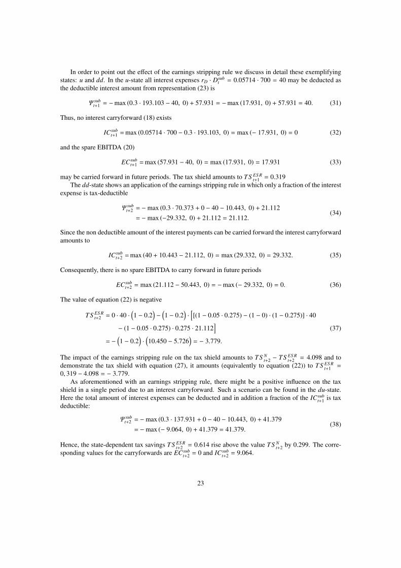
In order to point out the effect of the earnings stripping rule we discuss in detail these exemplifyingstates: u and dd. In the u-state all interest expenses rD · Dsub

t = 0.05714 · 700 = 40 may be deducted asthe deductible interest amount from representation (23) is

Ψ subt+1 = −max (0.3 · 193.103 − 40, 0) + 57.931 = −max (17.931, 0) + 57.931 = 40. (31)

Thus, no interest carryforward (18) exists

IC subt+1 = max (0.05714 · 700 − 0.3 · 193.103, 0) = max (− 17.931, 0) = 0 (32)

and the spare EBITDA (20)

EC subt+1 = max (57.931 − 40, 0) = max (17.931, 0) = 17.931 (33)

may be carried forward in future periods. The tax shield amounts to TS ES Rt+1 = 0.319

The dd-state shows an application of the earnings stripping rule in which only a fraction of the interestexpense is tax-deductible

Ψ subt+2 = −max (0.3 · 70.373 + 0 − 40 − 10.443, 0) + 21.112

= −max (−29.332, 0) + 21.112 = 21.112.(34)

Since the non deductible amount of the interest payments can be carried forward the interest carryforwardamounts to

IC subt+2 = max (40 + 10.443 − 21.112, 0) = max (29.332, 0) = 29.332. (35)

Consequently, there is no spare EBITDA to carry forward in future periods

EC subt+2 = max (21.112 − 50.443, 0) = −max (− 29.332, 0) = 0. (36)

The value of equation (22) is negative

TS ES Rt+2 = 0 · 40 ·

(1 − 0.2

)−

(1 − 0.2

)·[[(1 − 0.05 · 0.275) − (1 − 0) · (1 − 0.275)] · 40

− (1 − 0.05 · 0.275) · 0.275 · 21.112]

= −(1 − 0.2

)·(10.450 − 5.726

)= − 3.779.

(37)

The impact of the earnings stripping rule on the tax shield amounts to TS Nt+2 − TS ES R

t+2 = 4.098 and todemonstrate the tax shield with equation (27), it amounts (equivalently to equation (22)) to TS ES R

t+1 =

0, 319 − 4.098 = − 3.779.As aforementioned with an earnings stripping rule, there might be a positive influence on the tax

shield in a single period due to an interest carryforward. Such a scenario can be found in the du-state.Here the total amount of interest expenses can be deducted and in addition a fraction of the IC sub

t+1 is taxdeductible:

Ψ subt+2 = −max (0.3 · 137.931 + 0 − 40 − 10.443, 0) + 41.379

= −max (− 9.064, 0) + 41.379 = 41.379.(38)

Hence, the state-dependent tax savings TS ES Rt+2 = 0.614 rise above the value TS N

t+2 by 0.299. The corre-sponding values for the carryforwards are EC sub

t+2 = 0 and IC subt+2 = 9.064.

23

5. Implications for the Valuation of Tax Shields

Within the subsequent section, we aim at comparing the above discussed thin-capitalization and earn-ings stripping rules by determining their respective impact on the tax shield value. In order to illustratethe effect, we relate the values subject to the limited tax deductibility of interest to the tax shield valuewithout any limitation (VTS N

t ). For this numerical comparison we use the parameters from above, whichare summarized to: FCFU

t = 100, u = 1.4, q = 0.5, r f = 5.714%, α = 0, DTC

ETC = 4, τC = 27.5%,τP = 20%, τD = 20%, j = 1, h = 1, β = 0.3, and δ = 1, while we vary the total amount of debt from 200to 1, 200.

In order to quantify the difference between the tax shield values with and without the limiting rules,we calculate the percentage differences for the tax shield and the levered firm value. We define thepercentage difference of the tax shield values with and without limitation by

TS -difference =VTS N

t − VTS (.)t

VTS Nt

=∆TS

VTS Nt

(%), (39)

where the superscript (.) is in this respect the placeholder for the respective tax rule and the expression∆TS indicates the accumulated present values of the respective tax shield difference. A positive valueindicates the relative loss in tax shield value which results from a possible application of the discussedrules. Additionally, this reveals for values above 100% that due to respective tax treatment, the full taxsavings are lost and that debt financing has an overall negative value contribution. An equivalent analysiscan be conducted by determining the percentage difference for the levered firm values, i.e.

VL-difference =VL,N

t − VL,(.)t

VL,Nt

=∆TSVL,N (%). (40)

Table 4 provides an aggregated view on the effect of the thin-capitalization and earnings stripping rulesby showing the tax shield values (VTS N

t ) and the percentage share of the standard tax shield without anylimitation to the levered firm value ( VTS N

t

VL,Nt

), the direct impact of the respective tax rule (∆TS ) and theabove defined relative value differences. For completeness we depict the percentage share of the final tax

shield including interest limitation rules to the levered firm value without limitation rules ( VTS (.)t

VL,Nt

) as well

as the implied levered firm (VL,(.)t ) and equity values Et as well.

First, let us regard the tax shield without any limitations. In relation to the levered firm value the per-centage value contribution shows values between 0.13% and 0.8% with increasing debt values. Needlessto say that this small relative value contribution results from the fact that the tax shield is measured onthe parental level and therefore considers the double taxation effect of passing the subsidiary’s dividendson to the parent. Nevertheless, speaking in absolute terms, for a firm with a value of e 5 billion the taxshield would amount to e 40 million which is a non-neglectable value.

Second, we examine the impact of the interest limitation rules on the tax shield (and on the leveredfirm value). We observe that the earnings stripping rule is first applied at a debt level of 400, whilethe two cases of the thin-capitalization rule are applicable at a debt level of 500. The smallest relativedifference on the tax shield value can be recognized for the rec-case at a debt level of 500 with 1.074%(0.004%), while for the ESR-case the relative impact amounts to 2.032% (0.005%) already at a debtlevel of 400. The highest possible discount can be surveyed for the nor-case at a debt level of 1,200 with304.808% (2.412%). This shows that the impact of the limited interest deductibility exceeds the tax shieldwithout limitation and therefore indicates a tax advantage of equity financing. This effect can already berecognized at a debt level of 900 for the nor-case. The same effect can be observed for the ESR-case at adebt level of 1,000.

24

Tabl

e4

Tax

Shie

lds

and

Firm

Val

ues

depe

ndin

gon

the

Deb

tRat

iofo

rall

Inte

rest

Ded

uctio

nC

ases

Thi

sta

ble

show

sth

eim

pact

ofth

eth

in-c

apita

lizat

ion

and

earn

ings

stri

ppin

gru

les

onth

eta

xsh

ield

valu

e(V

TS

N t)

and

the

leve

red

firm

valu

e(V

L,N

t)

with

outa

nylim

itatio

nof

the

tax

dedu

ctib

ility

ofin

tere

stpa

ymen

ts.T

hepa

ram

eter

sof

the

num

eric

alex

ampl

ear

ese

tto

FC

Ft

=10

0,u

=1.

4,q

=0.

5,r f

=5.

714%

,α=

0,D

TC

ET

C=

4,τ C

=27.5

%,τ

P=

20%

,τD

=20

%,

j=1,

h=

1,β

=0.

3,an

dδ

=1,

whi

lew

eva

ryth

eto

tala

mou

ntof

debt

from

200

to1,

200.∆

TS

show

sth

ere

spec

tive

valu

esfo

rthe

cons

ider

edta

xru

les,

VT

SN t

VL,

Nt

the

valu

eco

ntri

butio

nof

the

tax

shie

ldw

ithou

tlim

itatio

non

the

over

allfi

rmva

lue,

VT

SN t−

VT

S(.) t

VT

SN t

and

VL,

Nt−

VL,

(.)t

VL,

Nt

(%)a

sdi

scus

sed

inse

ctio

n5

with

inth

eeq

uatio

n(3

9)an

d(4

0).

D(d

ebtr

atio

(%))

VT

SN t

VT

SN t

VL,

Nt

(%)

case

∆T

S=

∑ PV

(EQ t

[max

(.)])

∑ PV

(EQ t

[TS

N s−

TS

ES

Rs

])

VT

SN t−

VT

S(.) t

VT

SN t

(%)

VL,

Nt−

VL,

(.)t

VL,

Nt

(%)

VT

SN t−∆

TS

VL,

Nt

(%)

VL,

(.)t

E(.) t

200

(16.

66%

)1.

595

0.13

3re

c/n

or/E

SR0.

000

0.00

00.

000

0.13

312

01.5

9510

01.5

95

300

(25.

00%

)2.

393

0.19

9re

c/n

or/E

SR0.

000

0.00

00.

000

0.19

912

02.3

9390

2.39

3

400

(33.

33%

)3.

190

0.26

5re

c/n

or0.

000

0.00

00.

000

0.26

512

03.1

9080

3.19

0

ESR

0.06

52.

032

0.00

50.

260

1203

.125

803.

125

500

(41.

66%

)3.

988

0.33

1re

c0.

043

1.07

40.

004

0.32

812

03.9

4570

3.94

5

nor

1.20

730

.267

0.10

00.

231

1202

.781

702.

781

ESR

0.60

115

.081

0.05

00.

281

1203

.386

703.

386

600

(50.

00%

)4.

785

0.39

7re

c0.

054

1.12

90.

004

0.39

312

04.7

3160

4.73

1

nor

1.46

930

.706

0.12

20.

276

1203

.316

603.

316

ESR

1.49

931

.326

0.12

40.

273

1203

.286

603.

286

700

(58.

33%

)5.

583

0.46

3re

c0.

098

1.75

40.

008

0.45

512

05.4

8550

5.48

5

nor

3.76

667

.453

0.31

20.

151

1201

.817

501.

817

ESR

2.76

549

.531

0.22

90.

234

1202

.817

502.

817

800

(66.

66%

)6.

380

0.52

9re

c0.

151

2.36

30.

012

0.51

612

06.2

2940

6.22

9

nor

6.21

097

.333

0.51

50.

014

1200

.170

400.

170

ESR

4.41

769

.238

0.36

60.

163

1201

.963

401.

963

900

(75.

00%

)7.

178

0.59

5re

c0.

307

4.28

00.

025

0.56

912

06.8

7030

6.87

0

nor

9.62

213

4.05

40.

797

0.20

411

97.5

5629

7.55

6

ESR

6.48

690

.367

0.53

70.

058

1200

.691

300.

691

1000

(83.

33%

)7.

975

0.66

0re

c0.

542

6.79

10.

045

-0.6

1612

07.4

3320

7.43

3

nor

15.5

8419

5.41

31.

290

-0.6

3811

92.3

9119

2.39

1

ESR

8.90

111

1.61

40.

737

-0.0

7711

99.0

7419

9.07

4

1200

(100.0

0%)

9.57

00.

792

rec

1.06

611

.137

0.08

8-0

.704

1208

.504

10.0

00

nor

29.1

7030

4.80

82.

412

-1.6

6011

80.4

0010

.000

ESR

14.4

4315

0.91

61.

194

-0.4

0811

95.1

2710

.000

25

Finally, we compare the different influences of the respective cases. The rec-case shows the smallestrelative impact with values up to 11.137% (0.088%). As a direct result of the reclassification of non-deductible interest as dividend payments, this implies that the reclassified part of the interest payments isequally taxed as if the respective proportion of debt would have been equity financed (or financed by debtfrom a third party). In contrast to this, in the nor- and ESR-case, the non-deductible part of the interestpayments remains taxed as interest income which is taxed at a higher effective tax rate (due to a higher taxbase than dividend income). As already touched above, the earnings stripping rule applies at a lower debtlevel (400) than thin-capitalization rules (500), while the nor-case already causes the highest reduction onthe tax shield at a debt level of 700.

Overall, we find that thin-capitalization and earnings stripping rules have an important impact on thetax shield and in turn on the levered firm value. Evidently, with increasing leverage the value discounton the tax shield increases as well. In our example the relative impact on the tax shield varies between1 and 305%. Moreover, due to the different definitions of the earnings stripping and thin-capitalizationrules, any comparison among the rules has to be based on the major parameters, i.e. the EBITDA and thedebt-to-equity ratio respectively. Summarizing, for firms with high leverage it is important to considerthe effects of limited interest tax deductibility.

6. Conclusions

This paper analyzes the valuation of tax shields when specific tax rules limit the tax deductibility ofinterest payments on debt. Focussing on the specific tax codes of the EU-15 countries, we aim at setting upa theoretical framework that enables us to compare thin-capitalization rules limiting the tax deductibilityof interest payments originating from intragroup financing and earnings stripping rules. We are able toprovide a tractable tax shield and firm valuation model that includes the possibility of a limitation of thetax deductibility of interest implied by the regarded tax codes.

We show how the necessary adjustments can be incorporated in a tax shield valuation frameworkconsidering personal taxes. Thereby, we provide a general framework how specific tax codes limitingthe tax deductibility of interest can be integrated and show the respective valuation equation for the EU-15 countries. The ‘new’ tax shield representation reveals that the present value of the payoff-functionconsidering a possible limitation of interest tax deductibility is subtracted from the standard tax shield.Depending on the tax code this payoff-function and in turn the overall tax shield shows a path-dependentfeature.

Furthermore, in our analysis we highlight that for firms with a low leverage, there is no or a rathersmall impact of thin-capitalization and earnings stripping rules on the tax shield value. Nevertheless, forfirms with a high leverage, the impact of these rules results in an important and non-neglectable discountin the tax shield value. In some of the cases we observe that the impact has as consequence that thebenefits from debt financing could turn into a disadvantage.

The results obtained are important not only for company valuation in business practice. Additionally,the paper contributes to the academic tax shield discussion and provides valuation equations that couldserve as a measure for the benefits of debt financing that play an important role in other research fieldssuch as capital structure. We believe that more research within the field of tax shield valuation is necessaryto fully understand its impact on the overall firm.

26

Appendix A Derivation of Tax Shield Equations and Explanations for Thin-Capitalization Rules

A.1 Tax shield equations for general parent-subsidiary financing without limitation rules

The after-tax income of an unlevered subsidiary is given by

FCFU,subt+1 =

(1 − τC

)· EBIT sub

t+1 + Deprt+1 − Invt+1,

where Deprt+1 denotes the depreciation and Invt+1 the investments. For simplicity purposes we setDeprt+1 = Invt+1. Thereby, the unlevered free cash flows are determined by

FCFU,subt+1 =

(1 − τC

)· EBIT sub

t+1 .

By distributing 100% of the subsidiary’s after tax income to the parent and assuming that only afraction y of the distributed dividend is taxable at the parent level, the after tax income of the parent isgiven by

FCFU,part+1 =

(1 − τC

)· EBIT par

t+1 +(1 − τC

)·(1 − y · τC

)· EBIT sub

t+1

=(1 − τC

)·[EBIT par

t+1 + (1 − y · τC) · EBIT subt+1

].

Hence, the after tax income of an individual investor of an unlevered firm is determined by

FCFUt+1 =

(1 − τC

)·(1 − τP

)·[EBIT par

t+1 + (1 − y · τC) · EBIT subt+1

].

The after-tax income of a levered subsidiary without limitations on the tax deductibility of interestpayments is given by

FCFL,subt+1 =

(1 − τC

)·(EBIT sub

t+1 − I subt+1

).

By distributing 100% of the subsidiary’s after-tax income to the parent and assuming that a proportiony of the distributed dividend is taxable at the parent level, the after tax income of the parent is calculatedby

FCFL,part+1 =

(1 − τC

)·[EBIT par

t+1 − Ipart+1 + (1 − α) · I sub

t+1

]+

(1 − τC

)·(1 − y · τC

)·(EBIT sub

t+1 − I subt+1

)=

(1 − τC

)·(EBIT par

t+1 − Ipart+1 + I sub

t+1 − α · Isubt+1 + EBIT sub

t+1 − I subt+1 − y · τC · EBIT sub

t+1 + y · τC · I subt+1

)=

(1 − τC

)·[EBIT par

t+1 − Ipart+1 + (1 − y · τC) · EBIT sub

t+1 − (α − y · τC) · I subt+1

].

The after tax income of an individual investor of a levered firm is given by

FCFLt+1 =


t+1

)·(1 − τD

)+

(1 − τC

)·(1 − τP

)·[EBIT par


t+1 − (α − y · τC) · I subt+1

].

In any case, the period specific tax savings are determined as difference between the levered and

27

unlevered free cash flows

TS Nt+1 = FCFL

t+1 − FCFUt+1

=(Ipart+1 + α · I sub

t+1

)·(1 − τD

)+

(1 − τC

)·(1 − τP

)·[EBIT par


t+1

− (α − y · τC) · I subt+1

]−

(1 − τC

)·(1 − τP

)·[EBIT par

t+1 + (1 − y · τC) · EBIT subt+1

]=


t+1

)·(1 − τD

)+

(1 − τC

)·(1 − τP

)·[− Ipar

t+1 − (α − y · τC) · I subt+1

]=


t+1

)·(1 − τD

)−

(1 − τC

)·(1 − τP

)·[Ipart+1 + (α − y · τC) · I sub

t+1

].

A.2 Tax shield equations for the rec-case

In case that a thin capitalization rule applies, the subsidiary’s after-tax income including the non-deductible interest expense I sub

t+1 − Ht+1 is defined as

FCFL,TC,subt+1 =

(1 − τC

)·(EBIT sub

t+1 − α · Isubt+1 − Ht+1

)−

[(1 − α) · I sub

t+1 − Ht+1

]= EBIT sub

t+1 − α · Isubt+1 − Ht+1 − τC · EBIT sub

t+1 + τC · α · I subt+1 + τC · Ht+1 − I sub

t+1 + α · I subt+1 + Ht+1

=(1 − τC

)· EBIT sub

t+1 − I subt+1 + τC ·

(α · I sub

t+1 + Ht+1

).

The after-tax income of the parent including the subsidiary’s dividend income in case of reclassifica-tion (rec) is given by

FCFL,rec,part+1 =

(1 − τC

)·(EBIT par

t+1 − Ipart+1 + Ht+1

)+

(1 − y · τC

)·[(1 − τC) · EBIT sub

t+1 − I subt+1 + τC · (α · I sub

t+1 + Ht+1) + (1 − α) · I subt+1 − Ht+1

]=

(1 − τC

)·(EBIT par


)+

(1 − y · τC


t+1 − I subt+1 + τC · α · I sub

t+1 + τC · Ht+1 + I subt+1 − α · I

subt+1 − Ht+1

]=

(1 − τC

)·(EBIT par


)+

(1 − y · τC


t+1 − (1 − τC) · α · I subt+1 − (1 − τC) · Ht+1

]=

(1 − τC

)·(EBIT par


)+

(1 − τC

)·(1 − y · τC

)·(EBIT sub

t+1 − α · Isubt+1 − Ht+1

)=

(1 − τC

)·[EBIT par

t+1 − Ipart+1 + Ht+1 + (1 − y · τC) · (EBIT sub

t+1 − α · Isubt+1 − Ht+1)

].

This in turn implies that the after-tax income of an individual investor of a levered firm is determinedby

FCFL,rect+1 =


t+1

)·(1 − τD

)+

(1 − τC

)·(1 − τP

)·[EBIT par

t+1 − Ipart + Ht+1

+ (1 − y · τC) · (EBIT subt+1 − α · I

subt+1 − Ht+1)

].

28

The tax shield under consideration of a thin-capitalization rule in the rec-case is calculated as

TS rect+1 = FCFL,rec

t+1 − FCFUt+1


t+1

)·(1 − τD

)+

(1 − τC

)·(1 − τP

)·[EBIT par


+ (1 − y · τC) · (EBIT subt+1 − α · I

subt+1 − Ht+1)

]−

(1 − τC

)·(1 − τP

)·[EBIT par

t+1 + (1 − y · τC) · EBIT subt+1

]=


t+1

)·(1 − τD

)+

(1 − τC

)·(1 − τP

)·[− Ipar

t + Ht+1 − (1 − y · τC) · (α · I subt+1 + Ht+1)

]=


t+1

)·(1 − τD

)−

(1 − τC

)·(1 − τP

)·[Ipart+1 + (1 − y · τC) · (α · I sub

t+1 + Ht+1) − Ht+1

]=


t+1

)·(1 − τD

)−

(1 − τC

)·(1 − τP

)·[Ipart+1 + (1 − y · τC) · α · I sub

t+1 − y · τC · Ht+1

].

To show the impact of deductible interest expenses (Ht+1) and non-deductible interest expenses(I sub,non

t+1 ), the tax shield, in case that Ipart+1 = 0 and α = 0 is defined as

TS rect+1 =

(1 − τC

)·(1 − τP

)· y · τC · Ht+1.

A.3 Tax shield equations for the nor-case

If there is no reclassification of the dividends (nor-case) the after tax income of the parent is given by

FCFL,nor,part+1 =

(1 − τC

)·[EBIT par

t+1 − Ipart+1 + (1 − α) · I sub

t+1

]+

(1 − y · τC


t+1 − I subt+1 + τC · (α · I sub

t+1 + Ht+1)]

=(1 − τC

)·[EBIT par

t+1 − Ipart+1 + (1 − α) · I sub

t+1

]+

(1 − y · τC


t+1 − (1 − α · τC) · I subt+1 + τC · Ht+1

]=

(1 − τC

)·(EBIT par

t+1 − Ipart+1

)+

(1 − τC

)·(1 − α

)· I sub

t

+(1 − y · τC


t+1 − (1 − α · τC) · I subt+1 + τC · Ht+1

]=

(1 − τC

)·(EBIT par

t+1 − Ipart+1

)+

(1 − α

)·(1 − τC

)· I sub

t+1

+(1 − τC

)·(1 − y · τC

)· EBIT sub

t+1 −(1 − α · τC

)·(1 − y · τC

)· I sub

t+1 +(1 − y · τC

)· τC · Ht+1

=(1 − τC

)·[EBIT par


t+1

]+

(1 − α

)·(1 − τC

)· I sub

t+1

−(1 − α · τC

)·(1 − y · τC

)· I sub

t+1 +(1 − y · τC

)· τC · Ht+1

=(1 − τC

)·[EBIT par


t+1

]−

[(1 − α · τC) · (1 − y · τC) − (1 − α) · (1 − τC)

]· I sub

t+1 +(1 − y · τC

)· τC · Ht+1.

Hence the after-tax income of an individual investor of a levered firm is given by

FCFL,nort+1 =


t+1

)·(1 − τD

)+

(1 − τP

)·

[(1 − τC

)·[EBIT par


t+1

]−

[(1 − α · τC) · (1 − y · τC) − (1 − α) · (1 − τC)

]· I sub

t+1 +(1 − y · τC

)· τC · Ht+1

].

29

The tax shield under consideration of a thin-capitalization rule in the nor-case is calculated as

TS nort+1 = FCFL,nor

t+1 − FCFUt+1


t+1

)·(1 − τD

)+

(1 − τP

)·[(

1 − τC

)·[EBIT par


t+1

]−

[(1 − α · τC) · (1 − y · τC) − (1 − α) · (1 − τC)

]· I sub

t+1 +(1 − y · τC

)· τC · Ht+1

]−

(1 − τC

)·(1 − τP

)·[EBIT par

t+1 + (1 − y · τC) · EBIT subt+1

]=

(1 − τD

)·(Ipart+1 + α · I sub

t+1

)+

(1 − τP

)·[− (1 − τC) · Ipar

t+1

− [(1 − α · τC) · (1 − y · τC) − (1 − α) · (1 − τC)] · I subt+1 + (1 − y · τC) · τC · Ht+1

]=


t+1

)·(1 − τD

)−

(1 − τP

)·[(1 − τC) · Ipar

t+1

+ [(1 − α · τC) · (1 − y · τC) − (1 − α) · (1 − τC)] · I subt+1 − (1 − y · τC) · τC · Ht+1

].

To show the impact of deductible interest expenses (Ht+1) and non-deductible interest expenses(I sub,non

t ), the tax shield in case that Ipart = 0 and α = 0 is defined as

TS nort+1 = −

(1 − τP

)·[(1 − y) · τC · (I sub,non

t+1 + Ht+1) − (1 − y · τC) · τC · Ht+1

]= −

(1 − τP

)·[(1 − y) · τC · I

sub,nont+1 − (1 − τC) · y · τC · Ht+1

]A.4 Demonstration for validitiy of TS N

t+1 − TS TCt+1 ≤ 0 when a thin-capitalization rule is not applicable

In case of a thin-capitalization rule the tax shield is defined in the rec- and nor-case as

TS rect+1 =


t+1

)·(1 − τD

)−

(1 − τC

)·(1 − τP

)·[Ipart+1 + (1 − y · τC) · α · I sub

t+1 − y · τC · Ht+1

]and

TS nort+1 =


t+1

)·(1 − τD

)−

(1 − τP

)·[(1 − τC) · Ipar

t+1


]for

Ht+1 = (1 − α) · rD · Dsubt ·

jh·

E subt

Dsubt·

DTC

ETC .

The thin-capitalization applies, if

DTC

ETC ≤h · Dsub

t

j · E subt

,

where DTC

ETC is the fixed safe haven ratio, that has to be exceeded, h · Dsubt and j · E sub

t are the applicabledebt and equity values for calculating the exceeding safe haven ratio.

The tax shield in case that a thin-capitalization rule applies is defined as

TS t+1 = TS Nt+1 −max

(TS N

t+1 − TS TCt+1, 0

).

30

In the following, we want to demonstrate, the universality of

TS Nt+1 − TS TC

t+1 ≤ 0

for the situation that a thin-capitalization rule does not apply. This is valid for

DTC

ETC ≥h · Dsub

t

j · E subt

.

First, we demonstrate for the rec-case:

0 ≥ TS Nt+1 − TS rec

t+1

0 ≥(Ipart+1 − α · I

subt+1

)·(1 − τD

)−

(1 − τC

)·(1 − τP

)·[Ipart+1 + (α − y · τC) · I sub

t+1

]−

[ (Ipart+1 + α · I sub

t+1

)·(1 − τD

)−

(1 − τC

)·(1 − τP

)·[Ipart+1 − Ht+1 + (1 − y · τC) · (α · I sub

t+1 + Ht+1)]]

0 ≥(1 − τC

)·(1 − τP

)·[− Ipar

t+1 − (α − y · τC) · I subt+1 + Ipar

t+1 − Ht+1 + (1 − y · τC) · (α · I subt+1 + Ht+1)

]0 ≥

(1 − τC

)·(1 − τP

)·[− Ipar

t+1 − α · Isubt+1 + y · τC · I sub

t+1 + Ipart+1 − Ht+1 + α · I sub

t+1 + Ht+1 − y · τC · α · I subt+1 − y · τC · Ht+1

]0 ≥

(1 − τC

)·(1 − τP

)·[y · τC · (1 − α) · I sub

t+1 − Ht+1

]0 ≥

(1 − τC

)·(1 − τP

)· y · τC ·

[(1 − α) · I sub

t+1 − Ht+1

]0 ≥

(1 − τC

)·(1 − τP

)· y · τC ·

[(1 − α) · rD · Dsub

t − (1 − α) · rD · Dsubt ·

jh·

E subt

Dsubt·

DTC

ETC

]0 ≥

(1 − τC

)·(1 − τP

)· y · τC ·

(1 − α

)· rD ·

(Dsub

t −jh· E sub

t ·DTC

ETC

)0 ≥ Dsub

t −jh· E sub

t ·DTC

ETC

jh· E sub

t ·DTC

ETC ≥ Dsubt

DTC

ETC ≥h · Dsub

t

j · E subt

(q.e.d.).

31

Now we demonstrate for the nor-case:

0 ≥ TS Nt+1 − TS nor

t+1

0 ≥(Ipart+1 − α · I

subt+1

)·(1 − τD

)−

(1 − τC

)·(1 − τP

)·[Ipart+1 + (α − y · τC) · I sub

t+1

]−


t+1

)·(1 − τD

)−

(1 − τP

)·[(1 − τC) · Ipar

t+1 + [(1 − α · τC) · (1 − y · τC) − (1 − α) · (1 − τC)] · I subt+1 − (1 − y · τC) · τC · Ht+1

]]0 ≥

(1 − τP

)·[− (1 − τC) · Ipar

t+1 − (1 − τC) · (α − y · τC) · I subt+1 + (1 − τC) · Ipar

t+1


]0 ≥

(1 − τP

)·[[(1 − α · τC) · (1 − y · τC) − (1 − α) · (1 − τC) − (α − y · τC) · (1 − τC)] · I sub

t+1 − (1 − y · τC) · τC · Ht+1

]0 ≥

(1 − τP

)·[I subt+1 − ·τCα · I sub

t+1 − y · τC · I subt+1 + y · τC · τC · α · I sub

t+1 − I subt+1 + α · I sub

t+1 + τC · I subt+1 − τC · α · I sub

t+1 − α · Isubt+1

+ y · τC · I subt+1 + τC · α · I sub

t+1 − y · τC · τC · I subt+1 − (1 − y · τC) · τC · Ht+1

]0 ≥

(1 − τP

)·[− τC · α · I sub

t+1 + y · τC · τC · α · I subt+1 + τC · I sub

t+1 − y · τC · τC · I subt+1 − (1 − y · τC) · τC · Ht+1

]0 ≥

(1 − τP

)· τC ·

[− α · I sub

t+1 + y · τC · α · I subt+1 + I sub

t+1 − y · τC · I subt+1 − (1 − y · τC) · Ht+1

]0 ≥

(1 − τP

)· τC ·

[(1 − α) · I sub

t+1 − y · τC · (1 − α) · I subt+1 − (1 − y · τC) · Ht+1

]0 ≥

(1 − τP

)· τC ·

[(1 − y · τC) · (1 − α) · I sub

t+1 − (1 − y · τC) · Ht+1

]0 ≥

(1 − τP

)·(1 − y · τC

)· τC ·

[(1 − α) · I sub

t+1 − Ht+1

]0 ≥

(1 − τP

)·(1 − y · τC

)· τC ·

[(1 − α) · rD · Dsub

t − (1 − α) · rD · Dsubt ·

jh·

E subt

Dsubt·

DTC

ETC

]0 ≥

(1 − τP

)·(1 − y · τC

)·(1 − α

)· τC · rD ·

[Dsub

t − Dsubt ·

jh·

E subt

Dsubt·

DTC

ETC

]0 ≥

(1 − τP

)·(1 − y · τC

)·(1 − α

)· τC · rD ·

[Dsub

t −jh· E sub

t ·DTC

ETC

]0 ≥ Dsub

t −jh· E sub

t ·DTC

ETC

DTC

ETC ·jh· E sub

t ≥ Dsubt

DTC

ETC ≥h · Dsub

t

j · E subt

(q.e.d.).

32

Appendix B Derivation of Tax Shield Equations and Explanations for Earnings Stripping Rules

In general, the after-tax income of an individual investor of an unlevered firm is given by

FCFUt+1 =

(1 − τC

)·(1 − τP

)·[EBIT par

t+1 + (1 − y · τC) · EBIT subt+1

].

The subsidiary’s tax shield including the deductible interest expense Ψ subt+1 is defined as

FCFL,ES R,subt+1 =

(1 − τC

)·(EBIT sub

t+1 − Ψsubt+1

)−

(I subt+1 − Ψ

subt+1

)= EBIT sub

t+1 − Ψsubt+1 − τC · EBIT sub

t+1 + τC · Ψsubt+1 − I sub

t+1 + Ψ subt+1

=(1 − τC

)· EBIT sub

t+1 − I subt+1 + τC · Ψ

subt+1 .

Hence, the after-tax income of the parent considering its own deductible interest income Ψ part+1 is given

by

FCFL,ES R,part+1 =

(1 − τC

)·[EBIT par

t+1 + (1 − α) · I subt+1 − Ψ

part+1

]+

(1 − y · τC


t+1 − I subt+1 + τC · Ψ

subt+1

]−

(Ipart+1 − Ψ

part+1

)=

(1 − τC

)·[EBIT par

t+1 + (1 − α) · I subt+1 − Ψ

part+1

]+

(1 − y · τC


t+1 − I subt+1 + τC · Ψ

subt+1

]− Ipar

t+1 + τC · Ψpart+1 .

This implies for the after-tax income of an individual investor of a levered firm is given by

FCFL,ES Rt+1 =


t+1

)·(1 − τD

)+

(1 − τP

)·

[(1 − τC

)·[EBIT par

t+1 + (1 − α) · I subt+1 − Ψ

part+1

]+

(1 − y · τC

)[(1 − τC) · EBIT sub

t+1 − I subt+1 + τC · Ψ

subt+1

]− Ipar

t+1 + τC · Ψpart+1

].

33

The tax shield under consideration of an earnings stripping rule is calculated as

TS ES Rt+1 = FCFL,ES R

t+1 − FCFUt+1


t+1

)·(1 − τD

)+

(1 − τP

)·

[(1 − τC

)·[EBIT par

t+1 + (1 − α) · I subt+1 − Ψ

part+1

]+

(1 − y · τC


t+1 − I subt+1 + τC · Ψ

subt+1

]− Ipar


]−

(1 − τC

)·(1 − τP

)·[EBIT par

t+1 + (1 − y · τC) · EBIT subt+1

]=


t+1

)·(1 − τD

)+

(1 − τP

)·[(1 − τC) · (1 − α) · I sub

t+1

− (1 − y · τC) · I subt+1 + (1 − y · τC) · τC · Ψ

subt+1 − Ipar


]=


t+1

)·(1 − τD

)+

(1 − τP

)·[[(1 − α) · (1 − τC) − (1 − y · τC)] · I sub

t+1

+ (1 − y · τC) · τC · Ψsubt+1 + τC · Ψ

part+1 − Ipar

t+1

]=


t+1

)·(1 − τD

)−

(1 − τP

)·[Ipart+1 − [(1 − α) · (1 − τC) − (1 − y · τC)] · I sub

t+1

− (1 − y · τC) · τC · Ψsubt+1 − τC · Ψ

part+1

]=


t+1

)·(1 − τD

)−

(1 − τP


t+1

− τC · Ψpart+1 − (1 − y · τC) · τC · Ψ

subt+1

].

To show the influence of an earnings stripping rule, we define the difference between the tax shieldwithout any interest limitation TS N

t+1 with the tax shield under consideration of an earnings stripping rule

34

TS ES Rt+1 as

TS Nt+1 − TS ES R

t+1 =(Ipart+1 + α · I sub

t+1

)·(1 − τD

)−

(1 − τC

)·(1 − τP

)·[Ipart+1 + (α − y · τC) · I sub

t+1

]−


t+1

)·(1 − τD

)−

(1 − τP


t+1

− (1 − y · τC) · τC · Ψsubt+1 − τC · Ψ

part+1

]]=

(1 − τP

)·[− (1 − τC) · Ipar

t+1 − (1 − τC) · (α − y · τC) · I subt+1

+ Ipart+1 + [(1 − y · τC) − (1 − α) · (1 − τC)] · I sub

t+1 − τC · Ψpart+1 − (1 − y · τC) · τC · Ψ

subt+1

]=

(1 − τP

)·[− Ipar

t+1 + τC · Ipart+1 − [(1 − τC) · (α − y · τC) − [(1 − y · τC) − (1 − α) · (1 − τC)]] · I sub

t+1

+ Ipart+1 − τC · Ψ

part+1 − (1 − y · τC) · τC · Ψ

subt+1

]=

(1 − τP

)·[τC · I

part+1 − (α − τC · α − y · τC + y · τ2

C − 1 + y · τC + 1 − α − τC + τC · α) · I subt+1

− τC · Ψpart+1 − (1 − y · τC) · τC · Ψ

subt+1

]=

(1 − τP

)·[τC · I

part+1 − (y · τ2

C − τC) · I subt+1 − τC · Ψ

part+1 − (1 − y · τC) · τC · Ψ

subt+1

]=

(1 − τP

)·[τC · I

part+1 − (y · τC − 1) · τC · I sub

t+1 − τC · Ψpart+1 − (1 − y · τC) · τC · Ψ

subt+1

]=

(1 − τP

)· τC ·

(Ipart+1 − (y · τC − 1) · I sub

t+1 − Ψpart+1 − (1 − y · τC) · Ψ sub

t+1

)=

(1 − τP

)· τC ·

[Ipart+1 + (1 − y · τC) · I sub

t+1 − Ψpart+1 − (1 − y · τC) · Ψ sub

t+1

]=

(1 − τP

)· τC ·

[Ipart+1 − Ψ

part+1 + (1 − y · τC) · (I sub

t+1 − Ψsubt+1 )

].

In comparison to a thin-capitalization rule, an earnings stripping rule can also have a positive influenceon the tax shield as non-deductible interest expenses can be carried forward and deduct the taxable incomein future periods.

35

References

Arzac, E. R. and Glosten, L. R., ‘A Reconsideration of Tax Shield Valuation’, European FinancialManagement, Vol. 11(4), 2005, pp. 453-461.

Buettner, T. Overesch, M., Schreiber, U. and Wamser, G., ‘The impact of thin-capitalization rules onthe capital structure of multinational firms. A reconsideration of tax shield valuation’, Journal ofPublic Economics, Vol. 96(11-12), 2012, pp. 930-938.

Cooper, I. A. and Nyborg, K. G., ‘The value of tax shields IS equal to the present value of tax shields’,Journal of Financial Economics, Vol. 81(1), 2006, pp. 215-225.

Cooper, I. A. and Nyborg, K. G., ‘Tax-Adjusted Discount Rates with Investor Taxes and Risky Debt’,Financial Management, Vol. 37(2), 2008, pp. 365-379.

Couch, R., Dothan, M. and Wu, W., ‘Interest Tax Shields: A Barrier Options Approach’, Review ofQuantitative Finance and Accounting, Vol. 39(1), 2012, pp. 123-146.

Dempsey, M., ‘Consistent Cash Flow Valuation with Tax-Deductible Debt: a Clarification’, EuropeanFinancial Management, Vol. 19(4), 2013, pp. 830-836.

Eberl, S., ‘Weitere Erkenntnisse zum Steuervorteil von Fremdkapital nach der Unternehmensteuer-reform 2008’, Zeitschrift fuer betriebswirtschaftliche Forschung, Vol. 61(3), 2009, pp. 251-282.

Fernandez, P., ‘The value of tax shields is NOT equal to the present value of tax shields’, Journal ofFinancial Economics, Vol. 73(1), 2004, pp. 145-165.

Fieten, P., Kruschwitz, L., Laitenberger, J., Loeffler, A., Tham, J., Vélez-Pareja, I. and Wonder, N.,‘Comment on “The value of tax shields is NOT equal to the present value of tax shields” ’, TheQuarterly Review of Economics and Finance, Vol. 45(1), 2005, pp. 184-187.

Graham, J. R., ‘How Big Are the Tax Benefits of Debt?’, Journal of Finance, Vol. 55(5), 2000, pp.1901-1941.

Graham, J. R., ‘Taxes and Corporate Finance: A Review’, Review of Financial Studies, Vol. 16(4), 2003,pp. 1075-1129.

Knauer, A., Lahmann, A., Pfluecke, M. and Schwetzler, B., ‘How Much Do Private Equity Funds BenefitFrom Debt-related Tax Shields?’, Journal of Applied Corporate Finance, Vol. 26(1), 2014, pp. 85-93.

Knauer, T. and Sommer, F., ‘Interest barrier rules as a response to highly leveraged transactions: Evi-dence from the 2008 German business tax reform’, Review of Accounting and Finance, Vol. 11(2),2012, pp. 206-232.

Koziol, C., ‘A simple correction of the WACC discount rate for default risk and bankruptcy costs’,Review of Quantitative Finance and Accounting, Vol. 42, 2013, pp. 653-666.

Massari, M., Roncaglio, F. and Zanetti, L., ‘On the Equivalence between the APV and the waccApproach in a Growing Leveraged Firm’, European Financial Management, Vol. 14(1), 2008,pp. 152-162.

Miles, J. A. and Ezzell, J. R., ‘The Weighted Average Cost of Capital, Perfect Capital Markets, andProject Life: A Clarification’, Journal of Financial and Quantitative Analysis, Vol. 15(3), 1980,pp. 719-730.

36

Miles, J. A. and Ezzell, J. R., ‘Reformulating Tax Shield Valuation: A Note’, Journal of Finance,Vol. 40(5), 1985, pp. 1485-1492.

Miller, M. H., ‘Debt and Taxes’, Journal of Finance, Vol. 32(2), 1977, pp. 261-275.

Modigliani, F. and Miller, M. H., ‘The Cost of Capital, Corporation Finance, and the Theory of Invest-ment’, The American Economic Review, Vol. 48(3), 1958, pp. 261-297.

Modigliani, F. and Miller, M. H., ‘Corporate Income Taxes and the Cost of Capital: A Correction’, TheAmerican Economic Review, Vol. 53(3), 1963, pp. 433-443.

Molnár, P. and Nyborg, K. G., ‘Tax-adjusted Discount Rates: a General Formula under Constant Lever-age Ratios’, European Financial Management, Vol. 19(3), 2013, pp. 419-428.

Myers, S. C., ‘Interactions of Corporate Financing and Investment Decisions - Implications for CapitalBudgeting’, Journal of Finance, Vol. 29(1), 1974, pp. 1-25.

Overesch, M. and Wamser, G., ‘Corporate tax planning and thin-capitalization rules: evidence from aquasi-experiment’, Applied Economics, Vol. 42(5), 2010, pp. 563-573.

Rasmussen, P. N., ‘Direct EU regulation for Private Equity and Hedge funds The real economy comesfirst’, Commission conference on private equity and hedge funds, February 2009.

van Binsbergen, J. H., Graham, J. R. and Yang, J., ‘The Cost of Debt’, Journal of Finance, Vol. 65(6),2010, pp. 2089-2136.

Weichenrieder, A. J. and Windschbauer, H., ‘Thin-capitalization rules and company responses experi-ence from German legislation’, CESifo working paper, 2008, p. 2456.

37

The Impact of Thin-Capitalization and Earnings Stripping ... ANNUAL MEETINGS/2015-… · The Impact...

Documents

Transcript of The Impact of Thin-Capitalization and Earnings Stripping ... ANNUAL MEETINGS/2015-… · The Impact...