1

The Impact of Payday Lending on Crimes

Chen Shen

Belk College of Business

University of North Carolina at Charlotte

Charlotte, NC 28262, United States

Email: cshen3@uncc.edu

Keywords: Payday lending, Crime, Predatory Lending

JEL Classification: G38, G51

2

The Impact of Payday Lending on Crimes

Abstract

Police departments located in states allowing payday lending report 14.34% more

property crimes than the police departments located in states not allowing payday lending.

I also find that the police departments located in counties bordering with states allowing

payday lending report more property crimes. Those results are driven by the financial

pressure induced by payday loans. Furthermore, the impact of payday lending concentrates

in areas with a higher proportion of the minority population.

Keywords: Payday lending, Crime, Predatory Lending

JEL Classification: G38, G51

3

1. Introduction

Does borrowing at high-interest rates do more harm than good to the borrowers? The

classical economic theory predicts that borrowing would make the borrowers at least

weakly better off as consumers reveal their preferences by borrowing. The behavioral

model suggests that borrowing does not necessarily improve the borrowers’ financial

welfare if the borrowers are irrational (Carrell and Zinman, 2014). Policymakers and

borrower rights advocate groups often argue that restricting access to expensive credit

protects the borrowers’ interests (Zinman, 2010). Payday lending is one of the controversial

and expensive credits that receive mixed responses from borrowers and policymakers (e.g.,

Melzer, 2011, Skiba and Tobacman, 2011, Morgan and Strain, 2008, and Morse, 2011.).

The payday lending literature has focused primarily on the borrowers’ financial welfare

but overlooked the social impacts of payday lending. In this paper, I study how payday

lending affects crimes. I find that payday lending increases property crimes.

Access to payday lending could affect crime through several different channels. The

social disorganization theory (Kubrin et al., 2011) suggests that the payday loan stores

decrease guardianship against crime by introducing strangers to the neighborhoods. Also,

the presence of payday loan stores shows a sign of physical disorder and economic distress

in the neighborhood (Kubrin et al., 2011; Lee et al., 2013).

The routine activity theory (Kubrin and Hipp, 2016) suggests that payday loan stores

install a large volume of cash in the neighborhood that attracts burglary and robbery of

which the cash income from such offenses often facilitates drug consumption. The

literature documents the positive relationship between cash and crimes. Wright et al. (2017)

4

find that the electronic benefit transfer (EBT) program1 had a negative and significant

effect on the overall crime rate and specifically for burglary, assault, and larceny crimes.

Finally, because of the high annual percentage rate (APR) and the single-payment

structure, payday loan borrowers often find it is necessary to renew their contracts when

their loans mature because of the difficulty to repay the entire balance. Each time a loan is

renewed, the borrower incurs relatively high fees, the burden of which over time

exacerbates the borrowers’ financial difficulties. The financial strain theory (Kubrin et al.,

2011) suggests that financially distressed payday loan borrowers may become crime

offenders. For instance, personal indebtedness increases crime (McIntyre and Lacombe,

2012), and neighborhoods subject to higher interest rates have more property crimes

(Garmaise and Moskowitz, 2006).

Identifying the causal impact of payday lending is challenging because it is often

difficult to isolate the exogenous variation in payday lending access (Gathergood et al.,

2019). For example, payday lenders often locate their stores in low-income areas (Bhutta,

2014). To mitigate this concern, I follow the literature and exploit the plausibly exogenous

variation generated by the state laws prohibiting or allowing payday lending (Melzer, 2011;

Carrell and Zinman 2014).

I collect the property crimes data from the Uniform Crime Reporting (UCR) Program.

The UCR Program collects statistics on the number of offenses2 known to law enforcement.

I choose the sample period from 1985 to 2014 because that is the complete dataset offered

1 Electronic benefit transfer (EBT) is an electronic system that allows state welfare departments to issue benefits via

a magnetically encoded payment card used in the United States. It reached nationwide operations in 2004. The

average monthly EBT payout is $125 per participant. 2 These offenses including murder and non-negligent homicide, rape, robbery, aggravated assault, burglary, motor

vehicle theft, larceny-theft, and arson.

5

by the UCR program. Using the difference-in-differences specification, I find that the

agencies3 located in states allowing payday lending report 14.34% more property crimes

than agencies located in states not allowing payday lending, which translates into

approximately 270 property crimes per agency per year. Breaking down the type of

property crimes, agencies located in states allowing payday lending report 13.88%, 14.91%,

and 14.22% more burglary, larceny-theft, and motor theft crimes than agencies located in

states not allowing payday lending, those numbers represent approximately 68 burglary

crimes, 132 larceny-theft crimes, and 37 motor theft crimes. Also, the results are consistent

when replacing the state and year fixed effects with the agency and year fixed effects.

To identify the channel through which payday lending increases property crimes, I

conduct a placebo test by replacing the dependent variable with the violent crimes. The

rationale behind this test is that if payday lending affects crimes through the non-financial

channel(s), then that channel(s) is likely to increase violent crimes as well. Nevertheless, I

find that payday lending does not affect violent crimes. This result confirms that payday

lending increases property crimes by imposing more financial pressure on its borrowers.

One concern is that the results of the difference in differences analysis could be driven

by the trend differences between states allowing and not allowing payday lending.

However, such an effect is likely to show up even before the passing of laws allowing

payday lending. I, therefore, conduct a dynamic analysis for the effect of payday lending

on property crimes. I find that the coefficient estimates are statistically insignificant before

the treated states allowing payday lending, suggesting that the effect of payday lending on

3 The UCR program refers police department as agency.

6

crimes is not driven by the pre-existing differences between states allowing and not

allowing payday lending.

A more subtle concern is that the unobservable state characteristics could drive the

payday lending laws and local crime simultaneously. For example, state-level budget

problems could motivate the states to adopt laws allowing payday lending, and at the same

time, the worsening budget problems could also impact crime rates. To ensure that the

effects of payday lending on property crimes are not driven by the state-level factors that

are correlated with the laws, I follow Melzer (2011) to construct an alternative measure for

payday lending, an indicator equal to one not only for the states allowing payday lending

but also for the agencies located in counties bordering with a state allowing payday lending.

After controlling for the state×year fixed effects to account for the contemporaneous local

shocks at the state level, I find that the agencies located near a state allowing payday

lending report 18.41% more property crimes than the agencies located further away,

suggesting that the effect of payday lending on crimes is not driven by the state-level

unobservable factors.

To further identify whether payday lending affects property crimes through the

financial pressure channel, I split my sample based on the local economic conditions. I find

that the impact of payday lending on property crimes is stronger in areas subject to low

economic conditions such as low household income, low-income per capita, high

unemployment rate, and high property rate. I find that the effects of payday lending on

crimes are stronger in 3 out of 4 sub-samples associated with lower economic conditions.

Barth et al. (2015) suggest that borrowers who have limited access to banks are likely to

use more payday loans. If their argument is valid, I predict that people will use more payday

7

loans in the areas subject to fewer banks. It is reasonable to assume that the effect of payday

lending on crimes is stronger in such areas. To test this assumption, I split my sample based

on the number of commercial bank branches. I find that the effects of payday lending on

crimes are similar in both sub-samples, suggesting that the effect of payday lending on

crimes does not change with accessibility to banks. Last, to explore who are the real victims

of the property crimes induces by payday lending, I split my sample based on the proportion

of minority populations. I find that the effect of payday lending on property crimes is

stronger in the areas subject to the higher proportion of the African American population.

This result suggests that African American communities suffer more from the negative

social impact (Induce more property crimes) of payday lending on property crimes.

Payday lending could not only affects the borrowers’ financial welfare4but also affects

other aspects of borrowers’ life. For example, payday lending could cause psychological

and health problems, such as chronic stress, which could motivate the borrowers to engage

in criminal activities (Pew Charitable Trusts, 2016). Using the payday loan stores data in

2013, Barth et al. (2020) find that that the presence of payday lenders may help reduce

property crimes as well as personal bankruptcies. Nevertheless, their results may suffer

from the endogeneity issue because they do not isolate the exogenous variation in payday

lending access. Also, their results may be biased because they only use one year of data.

The reason is that they may overlook some unobserved factors that only exist in 2013 that

increase property crimes and payday loan stores simultaneously. Cuffe (2013) finds that

4 The literature has explored the relationship between payday lending and household financial welfare. Skiba and

Tobacman (2011) find that successful first-time payday borrowing often results in additional loans and interest

payments in the future. Campbell, Martinez-Jerez, and Tufano (2012) find that payday lending increases involuntary

bank account closures. Melzer (2011) finds that payday lending leads to increased difficulty in paying the mortgage,

rent, and utility bills. Fitzpatrick and Coleman-Jensen (2014) find that payday loans help protect some households

from food insecurity. Karlan and Zinman (2010) find that restricting access to payday lending cause deterioration in

the overall financial conditions of households.

8

the access to payday lending in some counties of payday lending prohibiting states

(Massachusetts, New Jersey, and New York) induces more larceny, fraud, and forgery

crimes. Nevertheless, his results are restricted to the three states in the Northeastern region

of the United States. Also, he does not find any impact of payday lending on burglary and

other types of property crimes. Hynes (2012) investigates the relationship between payday

loans’ legality and bankruptcy from 1998 to 2009. He reports that payday lending decreases

property crimes; However, his results may suffer from the endogeneity issue because he

fails to control for the unobservable state characteristics that could drive the payday lending

laws and local crimes simultaneously. Also, he does not include the crime data before 1998

which is publicly available. Xu (2016) studies the effect of payday lending on

neighborhood crime rates in Chicago, Illinois. She finds that the property crime rate

declined by 1.77% in the first year after the adoption of the new law and 1.49% in the

second year. Just as Cuffe (2013) does, her study only focuses on a specific region, which

does not provide the overall effect of payday lending on the national level.

Because of the data limitation (Geographic and/or time horizon) and problematic

identifications, the literature fails to provide a robust estimation of payday lending on

property crimes on the national level. My paper is the first one to provide the effect of

payday lending on property crimes on a nationwide level with clear identification strategies.

Unlike previous literature, my paper suggests that payday lending increases all types of

property crimes. This result may act as an alarm to the people who are considering using

payday loans to solve their financial difficulties. Also, I explore the channel through which

payday lending affects property crimes – the financial pressure induced by payday loans.

9

My paper also contributes to the literature on property crime by providing another cause

for property crimes - payday lending. Previous studies focus on the impact of households’

financial welfare on property crimes. Harries (2006) finds that both property and violent

crimes were moderately correlated with population density, and these crimes largely

affected the same blocks. Using the data from the 2000 British Crime Survey and the 1991

UK census small area statistics, Tseloni (2005) finds that both household and area

characteristics, as well as selected interactions, explain a significant portion of the variation

in property crimes. Howsen and Jarrell (1987) find that the level of poverty, the degree of

tourism, the presence of police, the unemployment rate, and the apprehension rate affect

property crimes. Kelly (2006) finds that violent crimes and property crimes are positively

influenced by the percentage of female-headed families and by population turnover, and

negatively related to the percentage of the population aged 16-24. Sampson (1985) and

Patterson (1991) argue that absolute and relative poverty link to property crime only

through their association with family and community instability. Drug enforcement also

affects property crimes. Benson and Rasmussen (1992) find that the resource reallocations

accompanying strong drug law enforcement lead to more property crimes. Besides the

households’ financial welfare and drug enforcement, law enforcement also plays a role in

property crimes. Sjoquist (1973) finds that an increase in the probability of arrest and

conviction and an increase in the cost of crime (punishment) both result in a decrease in

the number of property crimes. Last, other factors such as temperature also affect property

crimes. Cohn and Rotton (2000) find that more crimes were reported during summer than

in other months.

10

The remainder of the paper proceeds as follows. Section 2 describes the data and

construction. Section 3 details the empirical strategy and the identifying assumptions.

Section 4 provides the main results on the effects of payday lending on property crimes

and addresses the identification challenges. Section 5 extends the analysis by comparing

the number of crimes reported by police departments located near a state that allows payday

lending with the number of crimes reported by police departments located further away.

Section 6 presents some cross-sectional tests on the relationship between payday lending

and property crimes. Section 7 concludes.

2. Sample construction and variable definitions

I collect the crime data from the Uniform Crime Reporting (UCR) program. The UCR

Program collects data on the number of offenses known to law enforcement. The crime

data is obtained from the data received from more than 18,000 cities, universities and

colleges, counties, states, tribals, and federal law enforcement agencies voluntarily

participating in the program. These offenses including murder and non-negligent homicide,

rape, robbery, aggravated assault, burglary, motor vehicle theft, larceny-theft, and arson.

They are serious crimes that occur with regularity in all areas of the country. My sample

period starts from 1985 to 2014. I choose this period because this is the complete property

crime dataset on the agency level collected by the UCR program.

2.1. The dependent variable

The UCR program reports eight crimes including murder and non-negligent homicide,

rape (legacy & revised) 5 , robbery, aggravated assault, burglary, motor vehicle theft,

5 rape statistics prior to 2013 have been reported according to the historical definitions, identified on the tool as

"Legacy Rape". Starting in 2013, rape data may be reported under either the historical definition, known as "legacy

rape" or the updated definition, referred to as "revised."

11

larceny-theft, and arson. In this paper, I mainly focus on the number of property crimes,

that is, the sum of burglary, larceny-theft, and motor theft crimes, reported by the agencies.

My sample is a panel dataset with agency-year level observations. The dependent variables

are the natural logarithm of the number of property crimes (Ln (No. of property crimes)),

the natural logarithm of the number of burglary crimes (Ln (No. of burglary crimes)), the

natural logarithm of the number of larceny-theft crimes (Ln (No. of larceny-theft crimes)),

and the natural logarithm of the number of motor theft crimes (Ln (No. of motor theft

crimes)).

2.2. State Laws of Payday Lending

Some states have laws that effectively prohibiting payday lending by imposing binding

interest rate caps on payday loans or consumer loans. Some other states explicitly outlaw

the practice of payday lending. For example, Georgia prohibits payday loans under

racketeering laws in 2005. New York and New Jersey prohibit payday lending through

criminal usury statutes. Arkansas’s state constitution caps loan rates at 17 percent annual

interest in 2005. Maine caps interest at 30 percent but permits tiered fees that result in up

to 261 percent annual rates for a two-week $250 loan. Oregon permits a one-month

minimum term payday loan at 36 percent interest less a $10 per $100 borrowed initial loan

fees in 1998. Just as many other laws in the United States, the payday lending law also

varies in states. These laws are generally well-enforced, if not always perfectly enforced

(King and Parrish 2010), and hence provide a good source of variation in the availability

of payday loans across states and over time. I list the detailed information of state

legislation for payday lending in table A.1. of the appendix. I define the main independent

12

variable, Allowedit, to be one if state i’s law does not prohibit the standard payday loan

contract in year t, and zero otherwise.

2.3. State level and county level control variables

I include several state-level and county-level control variables that correlate with

property crimes from several sources. At the state level, I collect GDP per capita, household

income, unemployment rate, and poverty rate from the Federal Reserve Bank of St. Louis.

To control for the state-level political influences on the legislation, I add dummy variables

indicating whether the majority of the statehouse/state senate is controlled by the

Democratic party. I also add a dummy variable indicating whether the governor belongs to

the Democratic party. I collect those data from the Ballotpedia.6 County-level control

variables, such as population, personal income, income per capita, and the number of job

opportunities offered, are collected from the current population survey of the United States

Census Bureau. I collect the data for minority populations at the county level from the

National Bureau of Economic Research (NBER). To match the county-level control

variables with the agency-year level observations, I first identify which county the agency

is located in, and then match the property crimes reported by the agency with the counties’

federal information processing standards (FIPS) code. I use the FIPS code to match the

county-level control variables with the agency-level property crime data.

[Insert Table 1 Here]

Table 1 provides descriptive statistics for the agency-year observations sample. All

variables are winsorized at the 1% and 99% levels. 7 I have 100,775 agency-year

6 https://ballotpedia.org/Main_Page. 7 The results are consistent if I use unwinsorized data.

13

observations. The average number of Property crimes reported by agencies is 2,180.

Among all categories of property crimes, the most reported crime is larceny-theft. The

average of Larceny-theft crimes is 1,420.

[Insert Table 2 Here]

Table 2 reports the univariate comparison of the dependent variables between the

agency-year observations allowing payday lending and the agency-year observations not

allowing payday lending. The former reports a higher number of property crimes. For

example, the difference in the average number of property crimes between the agency-year

observations allowing payday lending and the agency-year observations not allowing

payday lending is 94. The difference in the median number of property crimes between

those two groups is approximately 153.

3. Identification strategy

The controversy over payday lending has led to considerable variation in the state laws

governing the industry. Using those differences, I define an indicator Allowedit, to be one

if state i’s law does not prohibit the standard payday loan contract in year t, and zero

otherwise. Because my baseline regressions include state and year fixed effects, the

variation that identifies the effect of Allowedit comes from states that switch from allowing

to prohibiting payday credit or vice versa. Allowedit will deliver unbiased estimates of the

effect of payday lending as long as the political economy behind changes in Allowedit does

not separately influence or respond to, property crimes. In another word, my identification

assumption is that payday law changes are uncorrelated with the changes in unobserved

determinants of property crimes. This assumption is valid because states make changes to

payday lending laws for reasons other than fighting against the crimes. For example,

14

Minnesota starts allowing payday lending in 1995 because of the Consumer Small Loan

Lender Act (https://www.revisor.mn.gov/statutes/cite/47.60) which intends to avoid

residents borrowing money from the unlicensed lender. North Carolina bans payday

lending in 2001 because of the predatory nature of such loans - inducing financial pressure

to the borrowers in North Carolina.

Following Morgan et al. (2012), I study how the number of property crimes changes as

the state switches from allowing to prohibiting payday lending, or vice versa. To mitigate

the concern that my results are driven by the differences between states allowing and not

allowing payday lending, I construct a propensity score-matched sample. Specifically, I

proceed as follows. First, I create a panel dataset that contains the state-year level data

including the number of crimes, the dummy variable Allowedit, and several control

variables that are correlated with the number of crimes. Second, I define the treated group

as those state-year observations allowing payday lending and the control group as those

state-year observations not allowing payday lending. In this sample, 754 (49.346%) state-

year observations allow payday lending, and 776 (50.654%) state-year observations do not

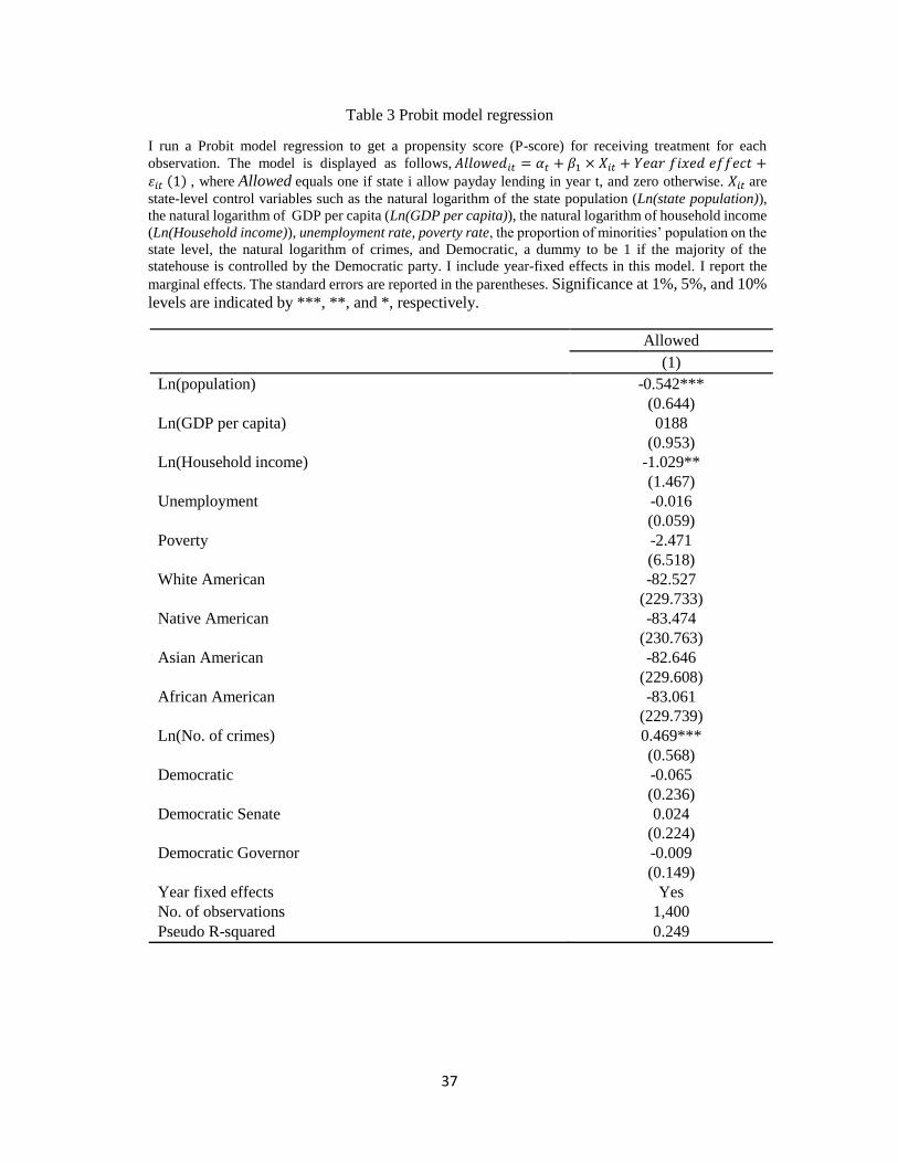
allow payday lending. Third, I run a Probit regression to estimate the propensity score (P-

score) for receiving the treatment for each observation as follows,

𝑃𝑟𝑜𝑏(𝐴𝑙𝑙𝑜𝑤𝑒𝑑𝑖𝑡) = 𝛼𝑡 + 𝛽1𝑋𝑖𝑡 + 휀𝑖𝑡 (1) ,

where 𝐴𝑙𝑙𝑜𝑤𝑒𝑑𝑖𝑡 is a dummy to be one if state i allows payday lending in year t, and zero

otherwise. The vector Xit is a set of state-level control variables that includes the natural

logarithm of state’s population (Ln (state population)), the natural logarithm of GDP per

capita (Ln (GDP per capita)), the natural logarithm of household income (Ln (Household

income)), Unemployment rate, Poverty rate, the percentage of the minority population, the

15

natural logarithm of the number of crimes (Ln (No. of crimes)), a dummy variable equals

one if the Democratic party controls the statehouse, a dummy variable equals one if the

Democratic party controls the senate, and a dummy variable indicates a Democratic

governor. I include year-fixed effects in this model and cluster the standard error at the

state level. I report the marginal effects in Table 3. The standard errors are reported in the

parentheses. After the Probit regression. I match the treated states with the control states

by using the closest P-score in the year that the treated states starting to allow payday

lending. This matching process is conducted without any replacement. The control state

not only includes the observations from states that never allowing payday lending but also

includes observations from states that allowing payday lending outside the ten years

window (-5, +5) around the matching treated state’s payday lending adoption year.

[Insert Table 3 Here]

This matching process generates 24 pairs of the treated-control states. I then use

the corresponding agency-year level observations of the treated-control states to test the

effects of payday lending on property crimes. I choose the ten years window, that is, from

five years before to five years after the treated states start allowing payday lending. Table

4 provides descriptive statistics for the matched sample used for this estimation. The

sample consists of 37,695 agency-year observations. The average number of Property

crimes is 2,401.12, which is comparable to the average number of Ln(property crime) in

the full agency-year observations sample. I then estimate the effect of payday lending on

property crimes with the following specification,

𝑃𝑟𝑜𝑝𝑒𝑟𝑡𝑦 𝑐𝑟𝑖𝑚𝑒𝑖𝑡 = 𝛼𝑠(𝑖) + 𝛼𝑡 + 𝛽1𝑇𝑟𝑒𝑎𝑡𝑖 × 𝑃𝑜𝑠𝑡𝑡 + 𝛽2𝑇𝑟𝑒𝑎𝑡𝑖 + 𝛽3𝑃𝑜𝑠𝑡𝑡 +

𝛾𝑋𝑠𝑡 + 𝛿𝑍𝑐𝑡 + 휀𝑖𝑡 (2) ,

16

where 𝑃𝑟𝑜𝑝𝑒𝑟𝑡𝑦 𝑐𝑟𝑖𝑚𝑒𝑖𝑡 is Ln (No. of property crimes) reported by agency i in year

t. 𝑇𝑟𝑒𝑎𝑡𝑖 equals one if the agency located in the treated states, and zero

otherwise. 𝑃𝑜𝑠𝑡𝑡 equals one for years after the treated state’s payday lending adoption year,

and zero otherwise. The vector Xst includes state-level control variables, such as the Ln

(Household income), Poverty rate, and Unemployment rate, and Ln (GDP per capita). The

vector 𝑍𝑐𝑡 includes county-level control variables, such as Ln (population), Ln (income per

capita), Ln (personal income), Ln (No. of jobs), the percentage of the minority population.

a dummy variable equals one if the Democratic party controls the statehouse, a dummy

variable equals one if the Democratic party controls the senate, and a dummy variable

indicates the Democratic governor. 𝛼𝑠(𝑖) is the state (agency) fixed effects that control for

any time-invariant factors across the state (agency) that are correlated with payday lending

laws. 𝛼𝑡 is the year fixed effects. Following Petersen (2009), I cluster the robust standard

errors at the state level because the payday lending laws vary at the state level. Under this

specification, 𝛽1captures the effect of payday lending laws on property crimes.

4. Results

4.1. Baseline difference-in-differences regressions

[Insert Table 4 Here]

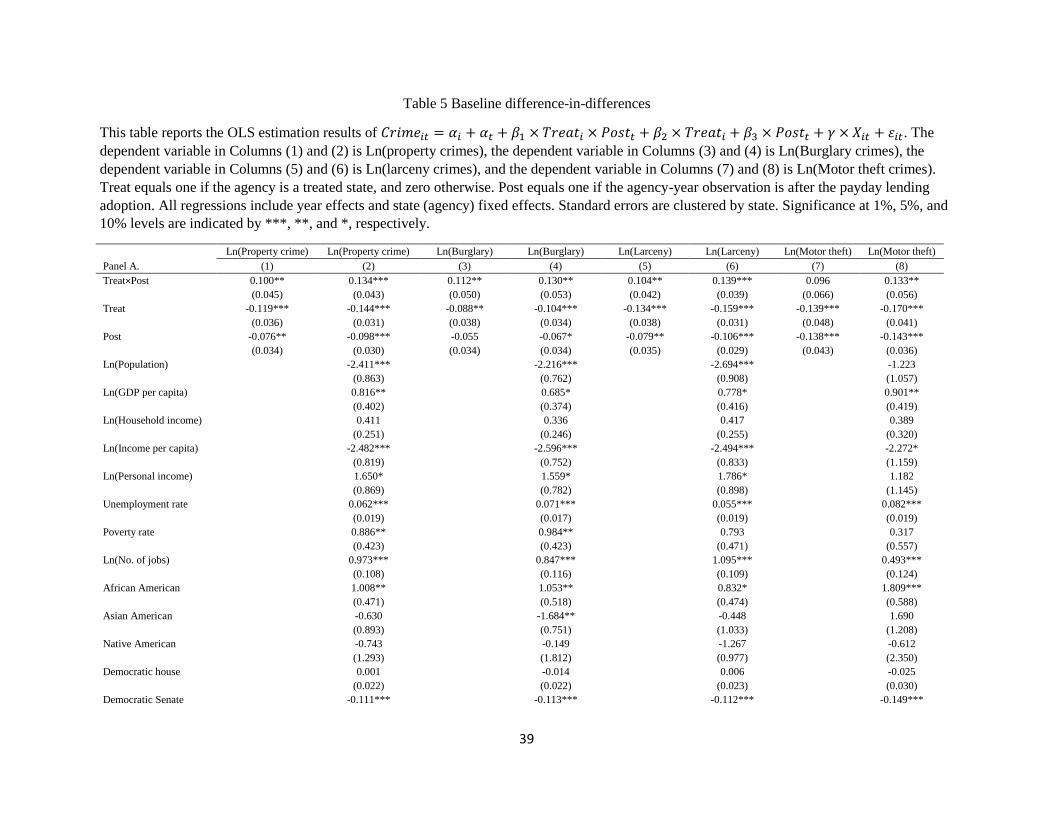
Table 5 reports the difference-in-differences results for estimating equation (2). I

control for state fixed effects and year fixed effects in panel A. The dependent variables

are Ln (No. of property crimes), Ln (No. of burglary crimes), Ln (No. of larceny-theft

crimes), and Ln (No. of motor theft crimes) in columns (1) to (8). The odd and even number

columns provide the results without and with the control variables. I include the results

without the control variables because if those variables are affected by the treatment

17

themselves then including them produces biased estimates (Angrist and Pischke, 2008). I

include the results with control variables to ensure that my results are robust. The standard

errors are reported in the parentheses. In panel A, the coefficient estimates of Treat×Post in

columns (1) and (2) are positive and statistically significant at the 10% and 5% levels.

Based on the estimates in column (2), agencies located in states allowing payday lending

report 14.34% more property crimes than agencies located in states not allowing payday

lending do, which amounts to approximately 270 property crimes based on the average

number of property crimes. The coefficient estimate on Treat×Post in column (4) is

positive and statistically significant at the 5% level, suggesting that the agencies located in

states allowing payday lending report 13.88% more burglary, which translates into

approximately 68 burglary crimes based on the average number of burglary crimes. The

coefficient estimates on Treat×Post in columns (5) and (6) are positive and significant at

the 5% and 1% levels, suggesting that the agencies located in states allowing payday

lending report 14.91% (or 132) more larceny-theft crimes than the agencies located in the

states not allowing payday lending do. The coefficient estimate on Treat×Post in column

(8) is positive and significant at the 5% level, suggesting that agencies located in states

allowing payday lending report 14.22% (or 37) more motor theft crimes than agencies

located in states not allowing payday lending.

In panel B, I replace the state fixed effects with the agency fixed effects. I find that the

coefficient estimates of Treat×Post are still statistically significant in columns (1) and (2).

In terms of economic significance, based on column (2), agencies located in states allowing

payday lending report 6.40% more property crimes than agencies located in states not

allowing payday lending do. This is equivalent to 127 property crimes.

18

[Insert Table 5 Here]

To identify the channels through which the payday lending laws affect property crimes,

I perform a placebo test that replaces Ln (No. of property crimes) with Ln (No. of violent

crimes) in equation (2) as the dependent variable. If payday lending affects property crimes

through some non-financial channel(s), payday lending should increase violent crimes. If

payday lending affects crimes through the social disorganization or routine activities

channel, then the borrowers and the payday loan lenders are likely the victims of some

violent crimes associated with payday lending. The reason is that offenders of such crimes

often use violence to receive cash that facilitates the consumption of drugs and other bad

behaviors. Under this scenario, I predict that payday lending increases violent crimes.

Nevertheless, if payday lending affects property crimes through the financial channel, then

the borrowers are likely the offenders of property crimes. This is because they are trying

to fix their financial problems by breaking the law. Under this scenario, the borrowers are

more likely to avoid committing violent crimes because they don’t want to solve one

problem by creating a new and more serious problem.

[Insert Table 6 Here]

Table 6 presents the results of the placebo test. The dependent variables are Ln (No. of

violent crimes), Ln (No. of murder crimes), Ln (No. of rape crimes), Ln (No. of robbery

crimes), and Ln (No. of aggravated assault crimes). In contrast to the coefficient estimates

on Treat×Post in Table 5, the coefficient estimates on Treat×Post are much smaller and

statistically insignificant in all columns (except for column (5) in panel A), suggesting that

the increases in property crimes are driven by the financial pressure induced by payday

loans.

19

4.2. Identification challenges

The consistency of the difference-in-differences estimation depends on the parallel

trend assumption, that is, the outcome variables should have parallel trends in the absence

of treatment. To ensure that the difference-in-differences estimation is not driven by the

pre-existing trend differences between treated and control states, I perform the dynamic

analysis for the effect of payday lending laws on the number of property crimes.

Specifically, I interact each event year dummy with the treated state dummy, that is, I

estimate the following,

𝑃𝑟𝑜𝑝𝑒𝑟𝑡𝑦 𝑐𝑟𝑖𝑚𝑒𝑖𝑡 = 𝛼𝑠 + 𝛼𝑡 + 𝛼𝑗 + ∑ 𝛽𝑘𝑇𝑟𝑒𝑎𝑡 × 𝑌𝑒𝑎𝑟𝑘 + 𝛾𝑋𝑠𝑡 + 𝛿𝑍𝑐𝑡 + 휀𝑖𝑡𝑘=3𝑘=−3 (3),

where all variables are defined the same as those in equation (2), except for 𝑌𝑒𝑎𝑟𝑘, which

is a dummy variable equal to one if the observation is k years after the states allowing

payday lending, and zero otherwise. 𝛼𝑖 is the state (agency) fixed effects. 𝛼𝑡 is the year

fixed effects. 𝛼𝑗 is the payday lending adoption year fixed effects. In this model,

𝛽𝑘 ′𝑠 capture the difference between the effect of payday lending on property crimes in

year k and the effect of payday lending on property crimes in four and five years before the

states starting to allow payday lending.

If the effect of payday lending on property crimes is not driven by the pre-existing

differences between the treated and control states, I expect 𝛽𝑘′𝑠 to be small for k less than

zero, and 𝛽𝑘′𝑠 to be positive for k greater than zero. However, if the difference-in-

differences estimates are driven by the pre-existing differences between the treated and

control states, the 𝛽𝑘′𝑠 could be positive for some k less than zero.

[Insert Figure 1 Here]

20

Figure 1 plots the coefficient estimates and their 95% confidence intervals of 𝑇𝑟𝑒𝑎𝑡 ×

𝑌𝑒𝑎𝑟𝑘. The dependent variable is Ln (No. of property crimes). I find that 𝛽𝑘′𝑠 are all small

and statistically insignificant for k less than zero, but they become larger and statistically

significant for some k greater than zero. These results suggest that the difference-in-

differences regression estimation is unlikely to be driven by the pre-existing differences

between the treated and control states.

5. Counties close to states legalizing payday lending

The baseline regression delivers unbiased estimates of the effect of payday lending if

payday lending law changes are uncorrelated with changes in unobserved determinants of

crimes. The natural question for the baseline regression is whether the state legislators

target payday lending and crimes at the same time. For example, state-level budget

problems could motivate the states to adopt laws allowing payday lending, and at the same

time, the worsening budget problems could also impact crime rates. Also, the baseline

regression results may be biased by unobserved factors at the state level. To mitigate this

concern, I use the same method as Melzer (2021). First, I construct an alternative measure

– an indicator called 𝐴𝑐𝑐𝑒𝑠𝑠_𝑋_𝑌𝑐𝑡. The 𝐴𝑐𝑐𝑒𝑠𝑠_𝑋_𝑌𝑐𝑡 equal to one if the center of the

county c is located within X and Y miles of a state allowing payday lending in year t, and

zero otherwise. I use the state×year fixed effects to reduce the concern that political forces

jointly affect payday laws and crimes, as there is little reason to believe that legislators in

nearby states directly influence the number of crimes outside of their state. Furthermore,

to the extent that political decisions are correlated among adjacent states, the state×year

fixed effects in the regressions prevent this source of variation from affecting the

𝐴𝑐𝑐𝑒𝑠𝑠_𝑋_𝑌𝑐𝑡 coefficients. Second, to ensure that the effects of payday lending on crime

21

are not driven by the state-level factors that are correlated with the payday lending laws, I

include the state×year fixed effects to account for contemporaneous local shocks at the

state level.

I compare the number of property crimes reported by agencies located near a state

allowing payday lending with the number of crimes reported by agencies located further

away from the state allowing payday lending. In particular, I estimate the following

specification,

𝑃𝑟𝑜𝑒𝑝𝑟𝑡𝑦 𝑐𝑟𝑖𝑚𝑒𝑖𝑡 = 𝛼𝑠×𝑡 + 𝛽1𝐴𝑐𝑐𝑒𝑠𝑠_𝑋_𝑌𝑐𝑡 + 𝛾𝑍𝑐𝑡 + 휀𝑖𝑡 (4),

For example, Access_0_30ct equals one if the center of a county is located 30 miles or less

from a state allowing payday lending, and zero otherwise. Access_30_40ct equals one if

the center of a county is located between 30 and 40 miles from a state allowing payday

lending, and zero otherwise. The omitted variable is Access_40_plus. The 𝐴𝑐𝑐𝑒𝑠𝑠_𝑋_𝑌𝑐𝑡

measure varies within the state-year, but only in states prohibiting payday lending. In other

words, if the state-year allows payday lending, 𝐴𝑐𝑐𝑒𝑠𝑠_𝑋_𝑌𝑐𝑡 equals one for sure. If the

state-year does not allow payday lending, then the 𝐴𝑐𝑐𝑒𝑠𝑠_𝑋_𝑌𝑐𝑡 can be one for some

agencies located in the county which is close to a state allowing payday lending. Within

the state-year, the effect of 𝐴𝑐𝑐𝑒𝑠𝑠_𝑋_𝑌𝑐𝑡 on crimes is identified by comparing the number

of property crimes reported by the agencies near a state allowing payday lending with those

reported by the agencies located further away from states allowing payday lending.

I use Access_0_30ct and Access_30_40ct as the independent variables and Ln(No. of

property crimes), Ln(No. of burglary crimes), Ln(No. of larceny-theft crimes), and Ln(No.

of motor theft crimes) as the dependent variables to estimate equation (4). Access_0_30ct is

an effective measure of payday lending because the borrowers who reside in states

22

prohibiting payday lending but have access to payday lenders use payday loans.

Considerable pieces of evidence suggest that people cross into payday allowing states to

get loans. Spiller (2006) documents that Massachusetts residents travel to New Hampshire

to get loans. Appelbaum (2006) documents the build-up of payday loan stores along the

South Carolina-North Carolina border to serve customers from North Carolina, which

prohibits payday lending. Those papers also document that payday lenders cluster at such

borders, as one would expect if they face demand from across the border. Therefore, I

include Border, a dummy variable indicating whether the center of the county is located

within 25 miles of the state border, in equation (4). Border controls for general differences

between counties near a state border and other counties.

[Insert Table 7 Here]

Table 7 presents the results of estimating equation (4). The coefficient estimates on

Access_0_30ct in columns (1) and (2) are positive and statistically significant at the 5% and

10% levels. The coefficient estimates on Access_30_40ct are statistically insignificant in

all columns, suggesting that the impact of payday lending on property crimes decreases

with the distance to states allowing payday lending. The agencies located within 30 miles

of a state allowing payday lending report 18.41% more property crimes than agencies

located further away. Overall, the results suggest two things. First, the effect on property

crimes is not driven by the political forces that jointly affect payday laws and crimes.

Second, payday lending not only affects property crimes in states allowing payday lending

but also affects property crimes in counties that share a border with the state(s) allowing

payday lending.

[Insert Figure 2 Here]

23

Next, I perform the dynamic analysis for the effect of Access_0_30ct on property crimes.

To do this, I create event year dummies for Access_0_30ct around the year (5 years before

to 3 and more years after) states starting allowing payday lending. Figure 2 plots the

coefficient estimates and their 95% confidence intervals for Access_0_30. The 𝛽𝑘′𝑠 are

small and statistically insignificant for all k less than zero, but they become larger and

statistically significant for some k greater than zero, suggesting that the results of table 7

are not driven by the pre-existing differences between a pair of border sharing counties

(One locates in a state allowing payday lending and the other does not).

6. The cross-sectional tests

6.1. Local economic conditions

To further identify whether payday lending affects property crimes through the

financial pressure channel, I split the propensity score matched-sample into two

subsamples-the poor economic condition subsample and the wealthy economic condition

subsample. I then re-estimate equation (2) and test the difference between the coefficient

estimates of Treat×Post in the poor economic condition subsample and the wealthy

economic condition subsample.

[Insert Table 8 Here]

Table 8 presents the results of estimating equation (2) for the poor economic condition

and the wealthy economic condition subsamples. Panels A, B, C, and D split the sample

based on the state-year median of household income, income per capita, unemployment

rate, and poverty rate. I find that the coefficient estimates on Treat×Post are positive and

statistically significant in low household income, low-income per capita, high

unemployment rate, and high poverty rate subsamples.

24

The differences between the coefficient estimates of Treat×Post are statistically

significant for household income, income per capita, and employment rate subsamples.

These results further suggest that the impact of payday lending laws on property crimes is

driven by the financial pressure induced by payday loans.

6.2. The availability of other lenders

The lack of access to formal financing could also serve as another channel to induce

people to use more payday loans. For example, the lack of commercial banks motivates

borrowers to use more payday loans (Barth et al., 2015). Also, Payday loan storeowners

are likely to establish their businesses in areas with fewer commercial banks (Pew

Charitable Trusts, 2016). If those arguments are valid, I predict that people will use more

payday loans in the areas subject to fewer banks. Therefore, if the financial distress induced

by payday loans motivates payday loan borrowers to engage in property crimes, this effect

should be stronger in areas with fewer commercial banks.

I collect the number of commercial bank branches at the county level from the Federal

Deposit Insurance Corporation (FDIC). I split the propensity score matched-sample based

on the state-year median number of commercial bank branches. If the lack of commercial

banks motivates borrowers to use more payday loans, then the financial pressure induced

by payday loans is going to increase for the borrowers. Under this case, I expect to find a

stronger effect of payday lending on property crimes in the subsample subject with fewer

banks. If the lack of banks does not motivate people to use more payday loans, then the

financial pressure would not change. Under this case, the effect of payday lending on

crimes should be similar in both areas.

[Insert Table 9 Here]

25

Table 9 presents the results of estimating equation (2) on the higher number of

commercial bank branches and the lower number of commercial bank branches subsamples.

The coefficient estimate on Treat×Post is positive and significant in column (1) of both

subsamples. The coefficient estimate in the lower commercial bank branches subsample is

slightly greater than that in the higher commercial bank branches subsample (0.126 vs

0.115). Nevertheless, the difference between those two coefficient estimates is small and

statistically insignificant, suggesting that the lack of commercial banks does not motivate

people to use more payday loans.

6.3. Who are the real victims of the effect of payday lending

Stegman and Faris (2003) and King, Li, Davis, and Ernst (2005) find that payday

lenders are likely to concentrate on the areas subject to the higher minority population.

Also, the extensive literature on discrimination in credit markets (Boucher, Barham, and

Carter, 2005) suggests that African Americans and other minorities have less access to the

lenders such as commercial banks.

To test whether the minorities’ population suffers more from the impact of payday

lending on property crimes, I split the propensity score matched-sample into two

subsamples - a higher minority population subsample and a lower minority population

subsample and then re-estimate the equation (2). If as the literature suggests that payday

lenders clustered in the minorities’ communities, then I would expect that the effect of

payday lending on property crimes is stronger in higher minority population subsamples.

[Insert Table 10 Here]

Table 10 presents the results of estimating equation (2) on a higher minority population

and lower minority population subsamples. Panels A, B, C, and D split the sample based

26

on the state-year median of the proportion of the African American, Native American,

Asian American, and Latino American populations. I find that the differences between the

coefficient estimates of Treat×Post in panels A and D are positive. Also, the difference

between the coefficient estimates of Treat×Post in panels A is statistically significant. The

panels B and C suggest that coefficient estimates of Treat×Post are positive and significant

in the lower minority population subsamples. The difference between the coefficient

estimates of Treat×Post is statistically significant in panel C.

These results indicate that the impact of payday lending on property crimes is larger in

the African American communities. To explain this result, Stegman (2007) finds that

payday lenders cluster in African American communities. The California Department of

business oversight (DBO, 2016) shows that payday loan stores in the state are

disproportionately located in heavily African American neighborhoods. Also, the financial

institutions do not treat their African American clients equally because the commercial

banks using credit scores as a primary determinant of loan approval. Since the average

African Americans have lower credit scores than the average White Americans have (Ards

and Myers, 2001; Ross and Yinger 2002; Federal Reserve Board 2007), the African

Americans’ likelihood of getting a loan denied is higher. To explain the results in Panel C

for Asian Americans. Sun (1998) reports that Asian American families are likely to save a

higher proportion of their income. Therefore, payday loan store owners are less likely to

establish their businesses in those communities because the demand is lower.

7. Conclusion

This paper studies the impact of state-level payday lending regulations on property

crimes in the United States. Consistent with the financial strain theory, evidence from the

27

difference-in-differences regressions show that legalizing payday lending increases

property crimes. On average, the agencies located in states allowing payday lending report

13.65% more property crimes than the agencies located in states not allowing payday

lending do. Nevertheless, this impact does not hold for the violent crimes because the effect

is driven by the borrowers’ financial pressure. In other words, payday lending increases

property crimes mainly by financial distress.

To strength my identification strategy, I conduct a dynamic analysis of the effect of

payday lending on property crimes. My results suggest that the difference-in-differences

regressions are unlikely to be driven by the pre-existing differences between treated and

control states. To account for contemporaneous local shocks at the state level, I create an

alternative measure following Melzer (2011) and include state×year fixed effects. My

results still hold. Last, I perform several cross-sectional tests to identify the heterogeneity

of the adverse effect of payday lending on property crimes. My results confirm that (1) The

payday lending laws have an impact on property crimes through the financial pressure

channel. (2) Compare with White Americans, minorities such as African Americans are

the real victims of the adverse impact of payday lending.

The payday loans industry makes large amounts of money from people who live close

to the financial edge. The policy question is whether those borrowers should be able to take

out high-cost loans repeatedly, or whether they should have a better alternative. Critics of

payday lenders, including the Center for Responsible Lending, claim that the loans could

become a debt trap for people who live paycheck to paycheck. Nevertheless, if the

industry’s critics devote themselves to stopping payday lenders from capitalizing on the

financial troubles of low-income borrowers, they should look for ways to make suitable

28

forms of credit available. Perhaps a solution to payday lending could come from reforms

that are more moderate to the payday lending industry, rather than attempts to close them.

Some evidence suggests that smart regulation can improve the business for both lenders

and consumers. In 2010, Colorado reformed its payday-lending industry by reducing the

permissible fees, extending the minimum term of a loan to six months, and requiring that

a loan be repayable over time, instead of coming due all at once. Pew reports that half of

the payday stores in Colorado closed, but each remaining store almost doubled its customer

volume, and now payday borrowers are paying 42 percent less in fees and defaulting less

frequently, with no reduction in access to credit.

29

REFERENCE

Agarwal, Sumit, Paige Marta Skiba, & Jeremy Tobacman. (2009) Payday loans and credit

cards: New liquidity and credit scoring puzzles?. American Economic Review 99.2:

412-17.

Angrist, J. D., & Pischke, J. S. (2008). Mostly harmless econometrics: An empiricist's

companion. Princeton university press.

Appelbaum, B. (2006). Lenders find payday over the border. The Charlotte Observer, 10.

Ards, S. D., & Myers Jr, S. L. (2001). The color of money: Bad credit, wealth, and race.

American Behavioral Scientist, 45(2), 223-239.

Barth, J. R., Hilliard, J., & Jahera, J. S. (2015). Banks and payday lenders: Friends or foes?.

International Advances in Economic Research, 21(2), 139-153.

Barth, J. R., Hilliard, J., Jahera, J. S., Lee, K. B., & Sun, Y. (2020). Payday lending, crime,

and bankruptcy: Is there a connection?. Journal of Consumer Affairs.

Benson, B. L., Kim, I., Rasmussen, D. W., & Zhehlke, T. W. (1992). Is property crime

caused by drug use or by drug enforcement policy?. Applied Economics, 24(7),

679-692.

Biagi, B., & Detotto, C. (2014). Crime as tourism externality. Regional Studies, 48(4), 693-

709.

Boucher, S. R., Barham, B. L., & Carter, M. R. (2005). The impact of “market-friendly”

reforms on credit and land markets in Honduras and Nicaragua. World

Development, 33(1), 107-128.

Campbell, D., Martínez-Jerez, F. A., & Tufano, P. (2012). Bouncing out of the banking

system: An empirical analysis of involuntary bank account closures. Journal of

Banking & Finance, 36(4), 1224-1235.

Carrell, S., & Zinman, J. (2014). In harm's way? Payday loan access and military personnel

performance. The Review of Financial Studies, 27(9), 2805-2840.

Carter, S. P., Skiba, P. M., & Tobacman, J. (2011). Pecuniary mistakes? Payday borrowing

by credit union members. Financial literacy: implications for retirement security

and the financial marketplace, 145-157.

Chu, Y. (2018). Shareholder-creditor conflict and payout policy: Evidence from mergers

between lenders and shareholders. The Review of Financial Studies, 31(8), 3098-

3121.

Cohn, E. G., & Rotton, J. (2000). Weather, seasonal trends and property crimes in

Minneapolis, 1987–1988. A moderator-variable time-series analysis of routine

activities. Journal of Environmental Psychology, 20(3), 257-272.

Cuffe, H. E. (2013). Financing crime? Evidence on the unintended effects of payday

lending. Working Paper.

Fajnzylber, P., Lederman, D., & Loayza, N. (2002). Inequality and violent crime. The

journal of Law and Economics, 45(1), 1-39.

Fitzpatrick, K., & Coleman-Jensen, A. (2014). Food on the fringe: Food insecurity and the

use of payday loans. Social Service Review, 88(4), 553-593.

Foley, C. F. (2011). Welfare payments and crime. The review of Economics and Statistics,

93(1), 97-112.

Garmaise, M. J., & Moskowitz, T. J. (2006). Bank mergers and crime: The real and social

effects of credit market competition. the Journal of Finance, 61(2), 495-538.

30

Gathergood, J., Guttman-Kenney, B., & Hunt, S. (2019). How do payday loans affect

borrowers? Evidence from the UK market. The Review of Financial Studies, 32(2),

496-523.

Hannon, L., & DeFronzo, J. (1998). Welfare and property crime. Justice Quarterly, 15(2),

273-288.

Harries, K. (2006). Property crimes and violence in the United States: An analysis of the

influence of population density. UMBC Faculty Collection.

Howsen, R. M., & Jarrell, S. B. (1987). Some determinants of property crime: Economic

factors influence criminal behavior but cannot completely explain the syndrome.

American Journal of Economics and Sociology, 46(4), 445-457.

Hynes, R. (2012). Payday lending, bankruptcy, and insolvency. Washington & Lee Law

Review, 69, 607.

Karlan, D., & Zinman, J. (2010). Expanding credit access: Using randomized supply

decisions to estimate the impacts. The Review of Financial Studies, 23(1), 433-464.

Kelly, M. (2000). Inequality and crime. Review of Economics and Statistics, 82(4), 530-

539.

King, U., Li, W., Davis, D., & Ernst, K. (2005). Race matters: The concentration of payday

lenders in African-American neighborhoods in North Carolina. Center for

Responsible Lending, 22.

Kubrin, C. E., & Hipp, J. R. (2016). Do fringe banks create fringe neighborhoods?

Examining the spatial relationship between fringe banking and neighborhood crime

rates. Justice Quarterly, 33(5), 755-784.

Lee, A. M., Gainey, R., & Triplett, R. (2014). Banking options and neighborhood crime:

Does fringe banking increase neighborhood crime?. American Journal of Criminal

Justice, 39(3), 549-570.

Lin, M. J. (2008). Does unemployment increase crime? Evidence from US data 1974–2000.

Journal of Human resources, 43(2), 413-436.

Manning, M., Fleming, C. M., & Ambrey, C. L. (2016). Life satisfaction and individual

willingness to pay for crime reduction. Regional Studies, 50(12), 2024-2039.

McGahey, R. M. (1986). Economic conditions, neighborhood organization, and urban

crime. Crime and justice, 8, 231-270.

McIntyre, S. G., & Lacombe, D. J. (2012). Personal indebtedness, spatial effects, and crime.

Economics Letters, 117(2), 455-459.

Melzer, B. T. (2011). The real costs of credit access: Evidence from the payday lending

market. The Quarterly Journal of Economics, 126(1), 517-555.

Melzer, B. T., & Morgan, D. P. (2015). Competition in a consumer loan market: Payday

loans and overdraft credit. Journal of Financial Intermediation, 24(1), 25-44.

Morgan, D. P., & Strain, M. (2008). Payday holiday: How households fare after payday

credit bans. FRB of New York Staff Report, (309).

Morgan, D. P., Strain, M. R., & Seblani, I. (2012). How payday credit access affects

overdrafts and other outcomes. Journal of Money, Credit and Banking, 44(2‐3),

519-531.

Morse, A. (2011). Payday lenders: Heroes or villains?. Journal of Financial Economics,

102(1), 28-44.

Nilsson, A. (2004). Income inequality and crime: The case of Sweden (No. 2004: 6).

Working Paper.

31

Parrish, L., & King, U. (2009). Phantom demand: Short-term due date generates the need

for repeat payday loans. Working paper.

Patterson, E. B. (1991). Poverty, income inequality, and community crime rates.

Criminology, 29(4), 755-776.

Petersen, M. A. (2009). Estimating standard errors in finance panel data sets: Comparing

approaches. The Review of Financial Studies, 22(1), 435-480.

Phaneuf, D. J., Smith, V. K., Palmquist, R. B., & Pope, J. C. (2008). Integrating property

value and local recreation models to value ecosystem services in urban watersheds.

Land Economics, 84(3), 361-381.

Raphael, S., & Winter-Ebmer, R. (2001). Identifying the effect of unemployment on crime.

The Journal of Law and Economics, 44(1), 259-283.

Ross, S. L., & Yinger, J. (2002). The color of credit: Mortgage discrimination, research

methodology, and fair-lending enforcement. MIT press.

Sampson, R. J. (1985). Neighborhood and crime: The structural determinants of personal

victimization. Journal of research in crime and delinquency, 22(1), 7-40.

Sjoquist, D. L. (1973). Property crime and economic behavior: Some empirical results. The

American Economic Review, 63(3), 439-446.

Spiller, K. (2006). ’Payday loans’ do a booming business in NH. The Telegraph, 22.

Stegman, M. A. (2007). Payday lending. Journal of Economic Perspectives, 21(1), 169-

190.

Stegman, M. A., & Faris, R. (2003). Payday lending: A business model that encourages

chronic borrowing. Economic Development Quarterly, 17(1), 8-32.

Sun, Y. (1998). The academic success of East-Asian–American students—An investment

model. Social Science Research, 27(4), 432-456.

Tita, G. E., Petras, T. L., & Greenbaum, R. T. (2006). Crime and residential choice: a

neighborhood-level analysis of the impact of crime on housing prices. Journal of

quantitative criminology, 22(4), 299.

Trusts, P. (2016). From Payday to Small Installment Loans. The Pew Charitable.

Tseloni, A. (2006). Multilevel modeling of the number of property crimes: Household and

area effects. Journal of the Royal Statistical Society: Series A (Statistics in Society),

169(2), 205-233.

Wilcox, P., & Eck, J. E. (2011). Criminology of the unpopular: Implications for policy

aimed at payday lending facilities. Criminology & Pubic policy, 10, 473.

Wright, R., Tekin, E., Topalli, V., McClellan, C., Dickinson, T., & Rosenfeld, R. (2017).

Less cash, less crime: Evidence from the electronic benefit transfer program. The

Journal of Law and Economics, 60(2), 361-383.

32

Appendix A. Variable description

Variable Definition (data source)

Crime rates

Ln(Property crime) Natural logarithm of the number of property crimes (uniform crime report)

Ln(Burglary) Natural logarithm of the number of burglary crimes (uniform crime report)

Ln(Larceny theft) Natural logarithm of the number of larceny-theft crimes (uniform crime report)

Ln(Motor theft) Natural logarithm of the number of motor theft crimes (uniform crime report)

Ln(Violent crime) Natural logarithm of the number of violent crimes (uniform crime report)

Ln(Murder) Natural logarithm of the number of murder crimes (uniform crime report)

Ln(Rape) Natural logarithm of the number of rape crimes (uniform crime report)

Ln(Robbery) Natural logarithm of the number of robbery crimes (uniform crime report)

Ln(Assault) Natural logarithm of the number of assault crimes (uniform crime report)

Payday lending access

Allowed Dummy variable equals one if the agency locate in the state allowing payday

lending, and zero otherwise

Treat Dummy variable equals one if the agency is located in the treated states, and zero

otherwise

Post Dummy variable equals one if the year is greater than or equal to the first adoption

year of the treated states, and zero otherwise

Access_x_y Dummy variable equals one if the center of the county is located within X and Y

miles of a state that allows payday lending, and zero otherwise

Border Dummy variable equals one if the center of the county is located 25 miles of a state

border, and zero otherwise

Payday border Dummy variable equals one if the county is located in a range of 15 miles from a

state that allows payday lending, and zero otherwise

State characteristics

Ln(GDP per capita) Natural logarithm of GDP per capita (Federal Reserve Bank of St Louis)

Ln(Household income) Natural logarithm of median household income (Federal Reserve Bank of St Louis)

Poverty rate The ratio of the number of people (in a given age group) whose income falls below

the poverty line (Federal Reserve Bank of St Louis)

Unemployment The share of the labor force that is jobless, expressed as a percentage (Federal

Reserve Bank of St Louis)

State characteristics

Ln(Population) Natural logarithm of county population (U.S Census Bureau)

Ln(Income per capita) Natural logarithm of county income per capita (U.S Census Bureau)

Ln(Personal income) Natural logarithm of county personal income (U.S Census Bureau)

Ln(No. of jobs) Natural logarithm of the number of jobs offered in each county (U.S Census

Bureau)

Native American The proportion of the Native American population (National bureau of economic

research)

African American The proportion of the African American population (National bureau of economic

research)

Asian American The proportion of the Asian American population (National bureau of economic

research)

Latino American The proportion of the Latino American population (National bureau of economic

research)

Democratic house Dummy variable equals one if the majority of the statehouse is held by the

democratic party

Democratic senate Dummy variable equals one if the majority of the senate is held by the democratic

party

Democratic governor Dummy variable equals one if the governor is a Democratic party member

33

Table A.1.

The sample starts in 1985 and ends in 2014. Many states have laws that effectively prohibit payday lending by imposing

binding interest rate caps on payday loans or consumer loans. Some other states explicitly outlaw the practice of payday

lending. These laws prohibiting or discouraging payday lending are generally well-enforced, if not always perfectly

enforced (King and Parrish 2010), and hence provide a good source of variations in the availability of payday loans across

states and time. My primary sources of those laws are the laws themselves such as statutes, superseded statutes, and

session laws.

Table A.1.

Classifying payday lending laws, 1985–2014

State

Permitted at the

start of the

sample?

Change 1

Change

2

Change 3

Year Type Year Type Year Type

AK No 2004 Yes

AL No 1998 Yes

AZ No 2000 Yes 2006 No

AR No 1999 Yes 2001 No 2005 Yes

CA No 1997 Yes

CO Yes

CT No

DC No 1998 Yes 2007 No

DE No 1987 Yes

FL Yes

GA No 2001 Yes 2005 No

HI No 1999 Yes

ID No 2001 Yes

IL No 2000 Yes

IN No 1990 Yes

IA No 1998 Yes

KS No 1991 Yes 2005 No

KY No 2009 Yes

LA No 1990 Yes

ME Yes

MD No

MA No

MI No 2005 Yes

MN No 1995 Yes

MS No 1998 Yes

MO No 2002 Yes

MT No 1999 Yes

34

NE No 1993 Yes

NV Yes

NH No 2003 Yes

NJ No

NM Yes

NY No

NC No 1997 Yes 2001 No

ND Yes 1997 No 2001 Yes

OH No 1995 Yes

OK No 2003 Yes

OR No 1998 Yes

PA No

RI No 2001 Yes

SC No 1998 Yes

SD No 1990 Yes

TN No 1990 Yes

TX No 2001 Yes 2005 No

UT No 1999 Yes

VT Yes 2001 No

VA No 2002 Yes 2005 No 2009 Yes

WA No 1995 Yes 2005 No

WV No

WI Yes

WY No 1996 Yes

35

Table 1 Descriptive statistics

This table reports the summary statistics of the variables used in this paper. The variables are the number

of property crimes, the number of burglary crimes, the number of larceny crimes, the number of motor theft

crimes, the number of violent crimes, the number of murder crimes, the number of rape crimes, the number

of robbery crimes, the number of assault crimes; Allowed, dummy equals one if the state law does not

prohibit the standard payday loan contract, and zero otherwise; Allowed_x_y, dummy equals one if the

center of the county is located within X and Y miles of a state allowing payday lending, and zero otherwise;

Border, dummy variable indicating whether the center of the county is located within 25 miles of the state

border; The GDP per capita; The household income; The Poverty rate, percentage of household income

below the federal poverty line; Unemployment, The share of the labor force that is jobless, expressed as a

percentage; The county population; The county income per capita; The county personal income; The

number of jobs offered in each county; Native American, The proportion of Native American population;

African American, The proportion of African American population; Asian American, The proportion of

Asian American population; Latino American, The proportion of Latino American population

Variable N Mean Std. Dev P25 Median P75

Panel A. Crime

Property crime 100,775 2,179.654 8,602.477 367 720 1,584

Burglary crime 100,775 500.418 1,979.748 70 154 359

Larceny theft crime 100,775 1,419.979 5,059.971 254 502 1,091

Motor theft crime 100,775 260.329 1,749.651 17 42 117

Violent crime 100,775 311.257 2,177.549 22 58 163

Murder 100,775 3.822 28.918 0 0 2

Rape 100,775 18.554 70.022 2 5 14

Robbery 100,775 108.644 1,120.3 3 10 35

Assault 100,775 186.715 1,139.556 13 37 107

Panel B. Payday lending

regulation

Allowed 100,775 0.468 0.499

Access_0_30 100,775 0.501 0.500

Access_30+ 100,775 0.072 0.258

Border 100,775 0.381 0.486

Panel C. State-level

characteristics

GDP per capita 100,775 35,145.36 12,955.61 23,865 34,131 44,239

Household income 100,775 40,491.48 11,071.85 31,496 40,379 48,294

Poverty rate 100,775 0.128 0.032 0.107 0.127 0.155

Unemployment 100,775 6.129 1.920 4.800 5.800 7.200

Democratic 100,775 0.582 0.493

Democratic Senate 100,775 0.523 0.499

Democratic Governor 100,775 0.323 0.484

Panel D. County-level

characteristics

Population 100,775 680,357.4 1406,684 84,789 250,432 694,808

Income per capita 100,775 29,869.9 12,706.79 19,995 27,741 37,098

Personal income 100,775 22,100 42,800 1,967 6,824 22,900

No. of jobs 100,775 401,990.8 819,316.6 42,452 133,250 411,682

White American 100,775 0.841 0.119 0.774 0.870 0.935

Native American 100,775 0.008 0.014 0.002 0.004 0.008

Asian American 100,775 0.033 0.040 0.007 0.018 0.039

African American 100,775 0.108 0.108 0.023 0.066 0.144

Latino American 100,775 0.103 0.143 0.019 0.045 0.138

36

Table 2 Uni-variate comparison

This table reports the univariate comparison for the sample. Panel A reports the univariate comparison of

crimes between agencies located in states allowing payday lending and agencies located in states not

allowing payday lending. Panel B reports the univariate comparison of control variables on county-level

between agencies located in states allowing payday lending and agencies located in states not allowing

payday lending. Panel C reports the univariate comparison of control variables on state-level between

agencies located in states allowing payday lending and agencies located in states not allowing payday

lending. The sample contains all crime information in the UCR program database originated during the

calendar years 1985 through 2014.

Allowed=1 Allowed=0 Difference

N=41,015 N=59,760

Panel A. Crime Mean Median Mean Median Mean Median

Property crime 2,257.280 813.000 2,163.230 660.000 94.050*** 153.000***

Burglary 505.804 142.000 498.107 171.000 7.698** -29.000**

Larceny theft 1,496.730 576.000 1,392.950 459.000 103.780*** 117.000***

Motor theft 268.174 48.000 255.883 39.000 12.290** 9.000**

Violent crime 314.874 71.000 314.286 51.000 0.588*** 20.000***

Murder 4.036 1.000 3.679 0.000 0.357* 1.000*

Rape 20.792 7.000 17.368 4.000 3.424 3.000

Robbery 118.553 12.000 97.416 9.000 21.138** 3.000**

Assault 196.263 45.000 182.866 33.000 13.397* 12.000*

37

Table 3 Probit model regression

I run a Probit model regression to get a propensity score (P-score) for receiving treatment for each

observation. The model is displayed as follows, 𝐴𝑙𝑙𝑜𝑤𝑒𝑑𝑖𝑡 = 𝛼𝑡 + 𝛽1 × 𝑋𝑖𝑡 + 𝑌𝑒𝑎𝑟 𝑓𝑖𝑥𝑒𝑑 𝑒𝑓𝑓𝑒𝑐𝑡 +휀𝑖𝑡 (1) , where Allowed equals one if state i allow payday lending in year t, and zero otherwise. 𝑋𝑖𝑡 are

state-level control variables such as the natural logarithm of the state population (Ln(state population)),

the natural logarithm of GDP per capita (Ln(GDP per capita)), the natural logarithm of household income

(Ln(Household income)), unemployment rate, poverty rate, the proportion of minorities’ population on the

state level, the natural logarithm of crimes, and Democratic, a dummy to be 1 if the majority of the

statehouse is controlled by the Democratic party. I include year-fixed effects in this model. I report the

marginal effects. The standard errors are reported in the parentheses. Significance at 1%, 5%, and 10%

levels are indicated by ***, **, and *, respectively.

Allowed

(1)

Ln(population) -0.542*** (0.644)

Ln(GDP per capita) 0188 (0.953)

Ln(Household income) -1.029** (1.467)

Unemployment -0.016 (0.059)

Poverty -2.471 (6.518)

White American -82.527 (229.733)

Native American -83.474 (230.763)

Asian American -82.646 (229.608)

African American -83.061 (229.739)

Ln(No. of crimes) 0.469*** (0.568)

Democratic -0.065 (0.236)

Democratic Senate 0.024 (0.224)

Democratic Governor -0.009 (0.149)

Year fixed effects Yes

No. of observations 1,400

Pseudo R-squared 0.249

38

Table 4 Descriptive statistics for the matched sample

This table reports the summary statistics of the variables used in this paper. The variables are the number

of property crimes, the number of burglary crimes, the number of larceny crimes, the number of motor theft

crimes, the number of violent crimes, the number of murder crimes, the number of rape crimes, the number

of robbery crimes, the number of assault crimes; Allowed, dummy equals one if the state law does not

prohibit the standard payday loan contract, and zero otherwise; Allowed_x_y, dummy equals one if the

center of the county is located within X and Y miles of a state allowing payday lending, and zero otherwise;

Border, dummy variable indicating whether the center of the county is located within 25 miles of the state

border; The GDP per capita; The household income; The poverty rate, percentage of household income

below the federal poverty line; Unemployment, The share of the labor force that is jobless, expressed as a

percentage; The county population; The county income per capita; The county personal income; The

number of jobs offered in each county; Native American, The proportion of Native American population;

African American, The proportion of African American population; Asian American, The proportion of

Asian American population; Latino American, The proportion of Latino American population; Democratic,

a dummy to be 1 if the majority of the statehouse is controlled by the Democratic party.

Variable N Mean Std. Dev P25 Median P75

Panel A. Crime

Property crime 37,695 2,401.116 9,242.779 384 788 1,749

Burglary crime 37,695 546.835 2,040.211 74 170 403

Larceny theft crime 37,695 1,538.184 5,368.235 264 536 1,182

Motor theft crime 37,695 316.140 2,012.753 20 49 143

Violent crime 37,695 361.086 2,526.395 25 67 184

Murder 37,695 4.540 32.899 0 1 2

Rape 37,695 19.637 74.478 2 6 15

Robbery 37,695 128.246 1,217.265 3 12 42

Assault 37,695 220.316 1,363.641 15 45 125

Panel B. Payday lending

regulation

Treat 37,695 0.511 0.499

Post 37,695 0.562 0.496

Panel C. State-level

characteristics

GDP per capita 37,695 32,139.56 9,269.338 24,787 31,490 38,816

Household income 37,695 38,194.51 8,582.36 31,855 37,715 44,005

Poverty rate 37,695 0.133 0.031 0.110 0.131 0.158

Unemployment 37,695 5.791 1.715 4.700 5.500 6.500

Democratic 37,695 0.686 0.464

Democratic Senate 37,695 0.542 0.499

Democratic Governor 37,695 0.373 0.482

Panel D. County-level

characteristics

Population 37,695 817,430.9 1,720,942 85,473 260,812 781,265

Income per capita 37,695 27,110.65 10,391.72 19,495 25,012 32,227

Personal income 37,695 22,100 42,800 1,967 6,824 22,900

No. of jobs 37,695 473,111.3 976,935.5 41,922 141,083 456,522

White American 37,695 0.845 0.115 0.495 0.866 0.991

Native American 37,695 0.008 0.014 0.002 0.004 0.008

Asian American 37,695 0.034 0.040 0.007 0.018 0.042

African American 37,695 0.105 0.108 0.780 0.067 0.933

Latino American 37,695 0.107 0.142 0.021 0.047 0.140

39

Table 5 Baseline difference-in-differences

This table reports the OLS estimation results of 𝐶𝑟𝑖𝑚𝑒𝑖𝑡 = 𝛼𝑖 + 𝛼𝑡 + 𝛽1 × 𝑇𝑟𝑒𝑎𝑡𝑖 × 𝑃𝑜𝑠𝑡𝑡 + 𝛽2 × 𝑇𝑟𝑒𝑎𝑡𝑖 + 𝛽3 × 𝑃𝑜𝑠𝑡𝑡 + 𝛾 × 𝑋𝑖𝑡 + 휀𝑖𝑡. The

dependent variable in Columns (1) and (2) is Ln(property crimes), the dependent variable in Columns (3) and (4) is Ln(Burglary crimes), the

dependent variable in Columns (5) and (6) is Ln(larceny crimes), and the dependent variable in Columns (7) and (8) is Ln(Motor theft crimes).

Treat equals one if the agency is a treated state, and zero otherwise. Post equals one if the agency-year observation is after the payday lending

adoption. All regressions include year effects and state (agency) fixed effects. Standard errors are clustered by state. Significance at 1%, 5%, and

10% levels are indicated by ***, **, and *, respectively.

Ln(Property crime) Ln(Property crime) Ln(Burglary) Ln(Burglary) Ln(Larceny) Ln(Larceny) Ln(Motor theft) Ln(Motor theft)

Panel A. (1) (2) (3) (4) (5) (6) (7) (8)

Treat×Post 0.100** 0.134*** 0.112** 0.130** 0.104** 0.139*** 0.096 0.133** (0.045) (0.043) (0.050) (0.053) (0.042) (0.039) (0.066) (0.056)

Treat -0.119*** -0.144*** -0.088** -0.104*** -0.134*** -0.159*** -0.139*** -0.170*** (0.036) (0.031) (0.038) (0.034) (0.038) (0.031) (0.048) (0.041)

Post -0.076** -0.098*** -0.055 -0.067* -0.079** -0.106*** -0.138*** -0.143*** (0.034) (0.030) (0.034) (0.034) (0.035) (0.029) (0.043) (0.036)

Ln(Population) -2.411*** -2.216*** -2.694*** -1.223 (0.863) (0.762) (0.908) (1.057)

Ln(GDP per capita) 0.816** 0.685* 0.778* 0.901** (0.402) (0.374) (0.416) (0.419)

Ln(Household income) 0.411 0.336 0.417 0.389 (0.251) (0.246) (0.255) (0.320)

Ln(Income per capita) -2.482*** -2.596*** -2.494*** -2.272* (0.819) (0.752) (0.833) (1.159)

Ln(Personal income) 1.650* 1.559* 1.786* 1.182 (0.869) (0.782) (0.898) (1.145)

Unemployment rate 0.062*** 0.071*** 0.055*** 0.082*** (0.019) (0.017) (0.019) (0.019)

Poverty rate 0.886** 0.984** 0.793 0.317 (0.423) (0.423) (0.471) (0.557)

Ln(No. of jobs) 0.973*** 0.847*** 1.095*** 0.493*** (0.108) (0.116) (0.109) (0.124)

African American 1.008** 1.053** 0.832* 1.809*** (0.471) (0.518) (0.474) (0.588)

Asian American -0.630 -1.684** -0.448 1.690 (0.893) (0.751) (1.033) (1.208)

Native American -0.743 -0.149 -1.267 -0.612 (1.293) (1.812) (0.977) (2.350)

Democratic house 0.001 -0.014 0.006 -0.025 (0.022) (0.022) (0.023) (0.030)

Democratic Senate -0.111*** -0.113*** -0.112*** -0.149***

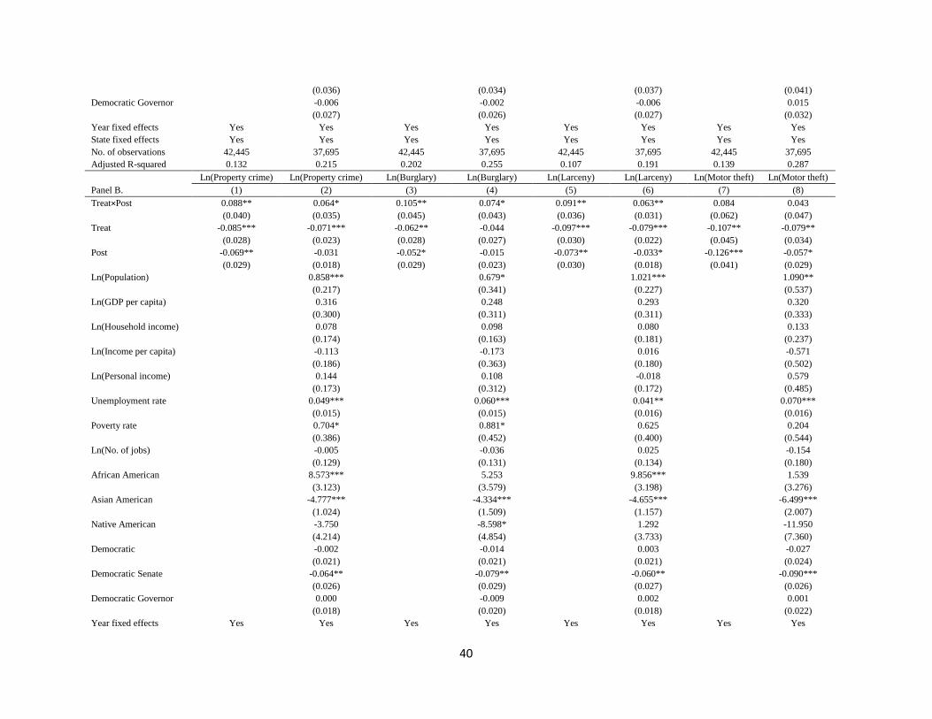
40

(0.036) (0.034) (0.037) (0.041)

Democratic Governor -0.006 -0.002 -0.006 0.015 (0.027) (0.026) (0.027) (0.032)

Year fixed effects Yes Yes Yes Yes Yes Yes Yes Yes

State fixed effects Yes Yes Yes Yes Yes Yes Yes Yes

No. of observations 42,445 37,695 42,445 37,695 42,445 37,695 42,445 37,695

Adjusted R-squared 0.132 0.215 0.202 0.255 0.107 0.191 0.139 0.287

Ln(Property crime) Ln(Property crime) Ln(Burglary) Ln(Burglary) Ln(Larceny) Ln(Larceny) Ln(Motor theft) Ln(Motor theft)

Panel B. (1) (2) (3) (4) (5) (6) (7) (8)

Treat×Post 0.088** 0.064* 0.105** 0.074* 0.091** 0.063** 0.084 0.043 (0.040) (0.035) (0.045) (0.043) (0.036) (0.031) (0.062) (0.047)

Treat -0.085*** -0.071*** -0.062** -0.044 -0.097*** -0.079*** -0.107** -0.079** (0.028) (0.023) (0.028) (0.027) (0.030) (0.022) (0.045) (0.034)

Post -0.069** -0.031 -0.052* -0.015 -0.073** -0.033* -0.126*** -0.057* (0.029) (0.018) (0.029) (0.023) (0.030) (0.018) (0.041) (0.029)

Ln(Population) 0.858*** 0.679* 1.021*** 1.090** (0.217) (0.341) (0.227) (0.537)

Ln(GDP per capita) 0.316 0.248 0.293 0.320 (0.300) (0.311) (0.311) (0.333)

Ln(Household income) 0.078 0.098 0.080 0.133 (0.174) (0.163) (0.181) (0.237)

Ln(Income per capita) -0.113 -0.173 0.016 -0.571 (0.186) (0.363) (0.180) (0.502)

Ln(Personal income) 0.144 0.108 -0.018 0.579 (0.173) (0.312) (0.172) (0.485)

Unemployment rate 0.049*** 0.060*** 0.041** 0.070*** (0.015) (0.015) (0.016) (0.016)

Poverty rate 0.704* 0.881* 0.625 0.204 (0.386) (0.452) (0.400) (0.544)

Ln(No. of jobs) -0.005 -0.036 0.025 -0.154 (0.129) (0.131) (0.134) (0.180)

African American 8.573*** 5.253 9.856*** 1.539 (3.123) (3.579) (3.198) (3.276)

Asian American -4.777*** -4.334*** -4.655*** -6.499*** (1.024) (1.509) (1.157) (2.007)

Native American -3.750 -8.598* 1.292 -11.950 (4.214) (4.854) (3.733) (7.360)

Democratic -0.002 -0.014 0.003 -0.027 (0.021) (0.021) (0.021) (0.024)

Democratic Senate -0.064** -0.079** -0.060** -0.090*** (0.026) (0.029) (0.027) (0.026)

Democratic Governor 0.000 -0.009 0.002 0.001 (0.018) (0.020) (0.018) (0.022)

Year fixed effects Yes Yes Yes Yes Yes Yes Yes Yes

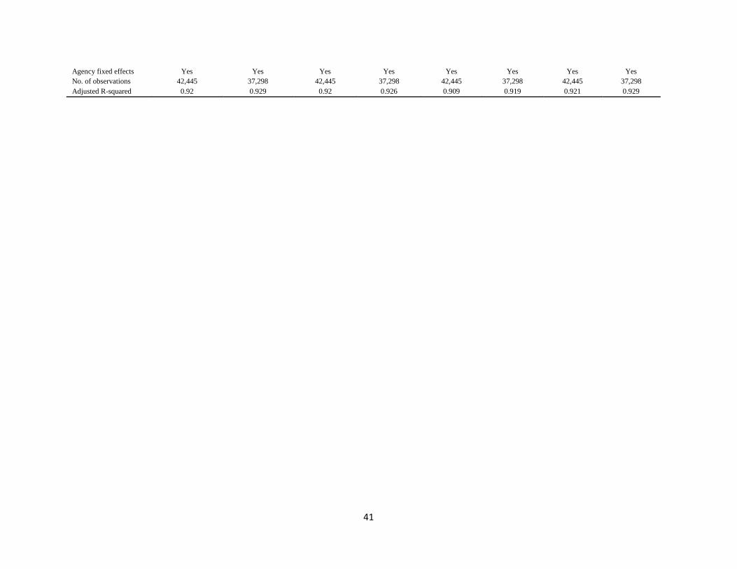
41

Agency fixed effects Yes Yes Yes Yes Yes Yes Yes Yes

No. of observations 42,445 37,298 42,445 37,298 42,445 37,298 42,445 37,298

Adjusted R-squared 0.92 0.929 0.92 0.926 0.909 0.919 0.921 0.929

42

Table 6 Placebo tests

This table reports the OLS estimation results of 𝐶𝑟𝑖𝑚𝑒𝑖𝑡 = 𝛼𝑖 + 𝛼𝑡 + 𝛽1𝑇𝑟𝑒𝑎𝑡𝑖 × 𝑃𝑜𝑠𝑡𝑡 + 𝛽2𝑇𝑟𝑒𝑎𝑡𝑖 + 𝛽3𝑃𝑜𝑠𝑡𝑡 + 𝛾𝑋𝑖𝑡 + 휀𝑖𝑡 . The dependent

variable in Columns (1) and (2) is Ln(Violent crimes), the dependent variable in Columns (3) and (4) is Ln(Murder crimes), the dependent variable

in Columns (5) and (6) is Ln(Rape crimes), the dependent variable in Columns (7) and (8) is Ln(Robbery crimes), and the dependent variable in

Columns (9) and (10) is Ln(Assault crimes). Treat equals one if the agency is a treated state, and zero otherwise. Post equals one if the agency-

year observation is after the payday lending adoption. All regressions include year effects and state (agency) fixed effects. Standard errors are

clustered by state. Significance at 1%, 5%, and 10% levels are indicated by ***, **, and *, respectively.

Ln(Violent

crime)

Ln(Violent

crime) Ln(Murder) Ln(Murder) Ln(Rape) Ln(Rape) Ln(Robbery) Ln(Robbery) Ln(Assault) Ln(Assault)

Panel A. (1) (2) (3) (4) (5) (6) (7) (8) (9) (10)

Treat×Post 0.057 0.039 -0.035 -0.036 0.065* 0.047 0.000 0.040 0.050 0.019 (0.044) (0.042) (0.028) (0.024) (0.036) (0.033) (0.059) (0.047) (0.044) (0.042)

Treat -0.081* -0.069** 0.011 0.010 -0.071* -0.056* -0.039 -0.062** -0.087* -0.067 (0.043) (0.034) (0.016) (0.014) (0.037) (0.029) (0.035) (0.030) (0.050) (0.042)

Post -0.042 -0.043 0.040** 0.038** -0.013 -0.033 0.009 -0.021 -0.048 -0.039

(0.035) (0.033) (0.015) (0.016) (0.022) (0.021) (0.039) (0.028) (0.040) (0.037)

Control variables No Yes No Yes No Yes No Yes No Yes

Year fixed effects

Yes Yes Yes Yes Yes Yes Yes Yes Yes Yes

State fixed

effects Yes Yes Yes Yes Yes Yes Yes Yes Yes Yes

No. of

observations 42,108 37,358 42,108 37,358 42,108 37,358 42,108 37,358 42,108 37,358

Adjusted R-squared 0.179 0.243 0.119 0.187 0.118 0.162 0.160 0.310 0.200 0.244

Ln(Violent

crime)

Ln(Violent

crime) Ln(Murder) Ln(Murder) Ln(Rape) Ln(Rape) Ln(Robbery) Ln(Robbery) Ln(Assault) Ln(Assault)

Panel B. (1) (2) (3) (4) (5) (6) (7) (8) (9) (10)

Treat×Post 0.044 -0.009 -0.037 -0.032 0.055 -0.012 -0.014 0.012 0.040 -0.028 (0.045) (0.038) (0.029) (0.020) (0.036) (0.037) (0.061) (0.042) (0.046) (0.044)

Treat -0.041 -0.001 0.028*** 0.017 -0.046 0.010 0.004 -0.009 -0.051 0.009 (0.028) (0.028) (0.009) (0.013) (0.031) (0.032) (0.030) (0.028) (0.034) (0.034)

Post -0.036 0.009 0.039** 0.037** -0.012 0.019 0.019 0.016 -0.043 0.017 (0.034) (0.026) (0.016) (0.015) (0.023) (0.025) (0.040) (0.022) (0.039) (0.032)

Control variables No Yes No Yes No Yes No Yes No Yes

Year fixed

effects Yes Yes Yes Yes Yes Yes Yes Yes Yes Yes

Agency fixed effects

Yes Yes Yes Yes Yes Yes Yes Yes Yes Yes

No. of

observations 42,108 36,961 42,108 36,961 42,108 36,961 42,108 36,961 42,108 36,961 Adjusted R-

squared 0.912 0.919 0.802 0.805 0.836 0.839 0.930 0.934 0.877 0.887

43

Table 7 Account for contemporaneous local shocks at the state level

This table reports the OLS estimation results of 𝐶𝑟𝑖𝑚𝑒𝑖𝑡 = 𝛼𝑖 + 𝛼𝑡 + 𝛽1𝐴𝑐𝑐𝑒𝑠𝑠 + 𝛾𝑋𝑖𝑡 + 휀𝑖𝑡 (4) . The dependent variable in Columns (1) and (2) is Ln(property

crimes), the dependent variable in Columns (3) and (4) is Ln(Burglary crimes), the dependent variable in Columns (5) and (6) is Ln(larceny crimes), and the

dependent variable in Columns (7) and (8) is Ln(Mother theft crimes). 𝐴𝑐𝑐𝑒𝑠𝑠_𝑋_𝑌𝑐𝑡 is a county-level indicator that equals one if the center of the county is

located within X and Y miles of a state allowing payday lending and zero otherwise. All regressions include state×year fixed effects. Standard errors are clustered

by state. Significance at 1%, 5%, and 10% levels are indicated by ***, **, and *, respectively.

Ln(Property

crime)

Ln(Property

crime)

Ln(Burglary

crime)

Ln(Burglary

crime)

Ln(Larceny

crime)

Ln(Larceny

crime)

Ln(Motor theft

crime)

Ln(Motor theft

crime)

(1) (2) (3) (4) (5) (6) (7) (8)

Access_0_30 0.174** 0.169* 0.062 0.060 0.049 0.075** 0.027 0.040

(0.084) (0.097) (0.047) (0.052) (0.067) (0.033) (0.104) (0.076)

Access_30_40 0.062 0.076 0.073 0.083 -0.059 0.023 -0.059 0.027

(0.144) (0.140) (0.120) (0.117) (0.130) (0.089) (0.158) (0.107)

Border 0.101 0.053 0.012 0.162**

(0.083) (0.060) (0.053) (0.064)

Control variables No Yes No Yes No Yes No Yes

State×Year fixed

effects Yes Yes Yes Yes Yes Yes Yes Yes

No. of observations 122,714 100,603 122,750 100,639 122,732 100,621 122,734 100,623

Adjusted R-squared 0.137 0.216 0.193 0.251 0.118 0.194 0.168 0.296

44

Table 8 Financial pressure

This table reports the OLS estimation results of 𝐶𝑟𝑖𝑚𝑒𝑖𝑡 = 𝛼𝑖 + 𝛼𝑡 + 𝛽1 × 𝑇𝑟𝑒𝑎𝑡𝑖 × 𝑃𝑜𝑠𝑡𝑡 + 𝛽2 × 𝑇𝑟𝑒𝑎𝑡𝑖 + 𝛽3 × 𝑃𝑜𝑠𝑡𝑡 + 𝛾 × 𝑋𝑖𝑡 + 휀𝑖𝑡 . for

subsample split by the state-median of household income, income per capita, employment rate, and poverty rate. The dependent variable in Columns

(1) and (2) is Ln(property crimes), the dependent variable in Columns (3) and (4) is Ln(Burglary crimes), the dependent variable in Columns (5) and

(6) is Ln(larceny crimes), and the dependent variable in Columns (7) and (8) is Ln(Motor theft crimes). Treat equals one if the agency is a treated

state, and zero otherwise. Post equals one if the agency-year observation is after the payday lending adoption. All regressions include year effects

and state (agency) fixed effects. Standard errors are clustered by state. Significance at 1%, 5%, and 10% levels are indicated by ***, **, and *,

respectively.

Panel A. Ln(Property crime) Ln(Property crime) Diff in (1) Panel B. Ln(Property crime) Ln(Property crime) Diff in (1)

Household income Low High Income per capita Low High

(1) (2) (3) (1) (2) (3)

Treat×Post 0.347*** -0.067* 0.414*** Treat×Post 0.169*** 0.074 0.095* (0.056) (0.036) P=0.0003 (0.052) (0.057) P=0.0943

Treat -0.213*** 0.014 Treat -0.165*** -0.123***

(0.068) (0.039) (0.035) (0.035)

Post -0.224*** 0.037 Post -0.098*** -0.085*

(0.044) (0.041) (0.03) (0.044)

Control variables Yes Yes Control variables Yes Yes

Year fixed effects Yes Yes Year fixed effects Yes Yes

State fixed effects Yes Yes State fixed effects Yes Yes

No. of observations 17,097 20,598 No. of observations 17,392 20,303

Adjusted R-squared 0.185 0.248 Adjusted R-squared 0.248 0.216 Panel C. Ln(Property crime) Ln(Property crime) Diff in (1) Panel D. Ln(Property crime) Ln(Property crime) Diff in (1)

Unemployment Low High Poverty Low High

(1) (2) (3) (1) (2) (3)

Treat×Post 0.094** 0.201** -0.107* Treat×Post 0.039 0.207** -0.168 (0.040) (0.075) P=0.081 (0.047) (0.092) P=0.201

Treat -0.044 -0.237*** Treat -0.038 -0.153

(0.030) (0.074) (0.053) (0.113)

Post -0.071*** -0.181*** Post -0.041 -0.119

(0.019) (0.057) (0.037) (0.081)

Control variables Yes Yes Control variables Yes Yes

Year fixed effects Yes Yes Year fixed effects Yes Yes

State fixed effects Yes Yes State fixed effects Yes Yes

No. of observations 21,231 16,464 No. of observations 20,424 17,271

Adjusted R-squared 0.213 0.198 Adjusted R-squared 0.197 0.188

45

Table 9 Access to commercial banks

This table reports the OLS estimation results of 𝐶𝑟𝑖𝑚𝑒𝑖𝑡 = 𝛼𝑖 + 𝛼𝑡 + 𝛽1𝑇𝑟𝑒𝑎𝑡𝑖 × 𝑃𝑜𝑠𝑡𝑡 + 𝛽2𝑇𝑟𝑒𝑎𝑡𝑖 + 𝛽3𝑃𝑜𝑠𝑡𝑡 + 𝛾𝑋𝑖𝑡 + 휀𝑖𝑡. For subsample split

by the state-median of no. of bank branches. The dependent variable in Columns (1) and (2) is Ln(property crimes. Treat equals one if the agency is

a treated state, and zero otherwise. Post equals one if the agency-year observation is after the payday lending adoption. All regressions include year

effects and state (agency) fixed effects. Standard errors are clustered by state. Significance at 1%, 5%, and 10% levels are indicated by ***, **, and

*, respectively.

Ln(Property crime) Ln(Property crime) Diff in (1)

Bank branches Low High

(1) (2) (3)

Treat×Post 0.126** 0.115 0.014

(0.054) (0.070) P=0.129

Treat -0.147*** -0.130***

(0.038) (0.046)

Post -0.108*** -0.088*

(0.037) (0.047)

Control variables Yes Yes

Year fixed effects Yes Yes

State fixed effects Yes Yes

No. of observations 14,799 22,896

Adjusted R-squared 0.234 0.201

46

Table 10 Minority population

This table reports the OLS estimation results of 𝐶𝑟𝑖𝑚𝑒𝑖𝑡 = 𝛼𝑖 + 𝛼𝑡 + 𝛽1 × 𝑇𝑟𝑒𝑎𝑡𝑖 × 𝑃𝑜𝑠𝑡𝑡 + 𝛽2 ×

𝑇𝑟𝑒𝑎𝑡𝑖 + 𝛽3 × 𝑃𝑜𝑠𝑡𝑡 + 𝛾 × 𝑋𝑖𝑡 + 휀𝑖𝑡. for subsample split by the state-median of the proportion of minority

populations. The dependent variable in Columns (1) and (2) is Ln(property crimes. Treat equals one if the

agency is a treated state, and zero otherwise. Post equals one if the agency-year observation is after the

payday lending adoption. All regressions include year effects and state (agency) fixed effects. Standard

errors are clustered by state. Significance at 1%, 5%, and 10% levels are indicated by ***, **, and *,

respectively.

Panel A. Ln(Property

crime)

Ln(Property

crime) Diff in (1) Panel B.

Ln(Property

crime)

Ln(Property

crime) Diff in (1)

African

American High Low

Native

American High Low

(1) (2) (3) (1) (2) (3)

Treat×Post 0.146*** 0.097* 0.049* Treat×Post 0.089 0.095* -0.006 (0.048) (0.051) P=0.086 (0.062) (0.052) P=0.471

Treat -0.171*** -0.124*** Treat -0.103** -0.084*

(0.030) (0.034) (0.044) (0.049)

Post -0.101*** -0.099** Post -0.053 -0.065**

(0.029) (0.038) (0.041) (0.032)

Control

variables Yes Yes Control

variables Yes Yes

Year fixed

effects Yes Yes Year fixed

effects Yes Yes

State fixed

effects Yes Yes State fixed

effects Yes Yes

No. of

observations 19,839 17,856 No. of

observations 17,943 20,816

Adjusted R-

squared 0.183 0.245

Adjusted R-

squared 0.261 0.184

Panel C. Ln(Property

crime)

Ln(Property

crime) Diff in (1) Panel D.

Ln(Property

crime)

Ln(Property

crime) Diff in (1)

Asian

American High Low

Latino

American High Low

(1) (2) (3) (1) (2) (3)

Treat×Post 0.03 0.158** -0.128** Treat×Post 0.118* 0.093* 0.025 (0.044) (0.062) P=0.047 (0.063) (0.050) P=0.243

Treat -0.057 -0.163*** Treat -0.150*** -0.112***

(0.039) (0.054) (0.041) (0.030)

Post -0.027 -0.102** Post -0.078* -0.085**

(0.031) (0.038) (0.043) (0.033)

Control

variables Yes Yes Control

variables Yes Yes

Year fixed

effects Yes Yes Year fixed

effects Yes Yes

State fixed

effects Yes Yes State fixed

effects Yes Yes

No. of

observations 20,788 17,971 No. of

observations 16,956 20,739

Adjusted R-

squared 0.223 0.211

Adjusted R-

squared 0.168 0.272

47

Figure 1

Figure 1 plots the coefficient estimates and their 95% confidence intervals of 𝑇𝑟𝑒𝑎𝑡 × 𝑌𝑒𝑎𝑟𝑘 for

equation (3). 𝑃𝑟𝑜𝑝𝑒𝑟𝑡𝑦 𝑐𝑟𝑖𝑚𝑒𝑖𝑡 = 𝛼𝑖 + 𝛼𝑡 + 𝛼𝑗 + ∑ 𝛽𝑘 × 𝑇𝑟𝑒𝑎𝑡 × 𝑌𝑒𝑎𝑟𝑘 + 𝛾 × 𝑋𝑖𝑡 + 휀𝑖𝑡𝑘=3𝑘=−3 (3),

The dependent variable is Ln (No. of property crimes). all variables are defined the same as those in

equation (2), except for Year, which equals one if the 𝑌𝑒𝑎𝑟𝑘 is k years after the adoption year, and

zero otherwise. All regressions include year effects and state (agency) fixed effects. Standard errors

are clustered by state. Significance at 1%, 5%, and 10% levels are indicated by ***, **, and *,

respectively.

48

Figure 2

Figure 2 plots the dynamic coefficient estimates and their 95% confidence intervals of

Access_0_30. The dependent variable is Ln (No. of property crimes). All variables are defined the same

as those in equation (2). All regressions include State×year fixed effects. Standard errors are clustered by

state. Significance at 1%, 5%, and 10% levels are indicated by ***, **, and *, respectively.