- 1 -

ERASMUS UNIVERSITY

ROTTERDAM ERASMUS SCHOOL OF ECONOMICS

MSc Economics & Business

Master Specialization Financial Economics

Sector: Energy Finance

The impact of fluctuations in the crude oil price on the stock

price of renewable energy companies, an impulse response

analysis

Author: Student Number: Date:

Bastiaan Moelands 346033 1 March, 2017

Burgemeester Oudlaan 50

3062 PA Rotterdam

The Netherlands

Thesis Supervisor: Co-reader:

Mehtap Kılıç Ronald Huisman

Professor of Business Economics Professor of Business Economics

Department of Economics Department of Economics

Rotterdam School of Economics Rotterdam School of Economics

Erasmus University Rotterdam Erasmus University Rotterdam

- 2 -

Abstract

The aim of this paper is to examine the dynamic interactions among the renewable energy

industry, oil price and technology companies and how they affect each other. This is done by

utilizing a self-made index of companies that are included in the EF-I index, the crude oil

price based on the WTI and Brent Blend and finally the Arca Tech 100 index. The sample

period of daily data is from 01/01/2010 up to and including 31/01/2016. The methodology

applied is the examination of the impulse response functions obtained by using a VAR model.

I find that after an impulse in the oil price, renewable energy companies show an upward

movement on in the subsequent days. Additionally, renewable energy companies react more

heavily to shocks in the technology index. From this finding, it can be concluded that

renewable energy companies are (still) more correlated to the underlying technology than to

their substitute product crude oil.

JEL Classification code: C12, Q21, E29

Keywords: Renewable Energy, Stock Performance, Technology, Oil Price, Fluctuations,

shocks, Vector-auto Regression Model, VAR, Impulse Response

- 3 -

I. Table of Contents

ABSTRACT ...................................................................................................................................... - 2 -

I. TABLE OF CONTENTS .................................................................................................................... - 3 - II. LIST OF ABBREVIATIONS ................................................................................................................ - 4 - III. LIST OF TABLES ........................................................................................................................... - 4 - IV. LIST OF FIGURES .......................................................................................................................... - 5 - V. LIST OF APPENDIX ....................................................................................................................... - 5 -

1 INTRODUCTION .................................................................................................................... - 6 -

2 ENERGY MARKET OVERVIEW ................................................................................................ - 9 -

2.1. FOSSIL FUEL BASED MARKET ...................................................................................................... - 9 - 2.2. RENEWABLE ENERGY MARKET ................................................................................................. - 10 - 2.3. THE INTERACTION BETWEEN RENEWABLE AND FOSSIL-FUEL GENERATED ENERGY ............................... - 12 -

3 THEORETICAL FRAMEWORK................................................................................................ - 12 -

3.1. THE ECONOMIC MODEL OF SUPPLY AND DEMAND........................................................................ - 13 - 3.2. THE EFFICIENT MARKET HYPOTHESIS ......................................................................................... - 13 - 3.3. LITERATURE REVIEW .............................................................................................................. - 14 -

3.3.1. Shocks in oil prices and the effect of renewable energy companies ..................... - 15 - 3.2.2. Shocks in oil prices and the effect on the consumption of renewable energy ...... - 18 -

4 EMPIRICAL METHODOLOGY ............................................................................................... - 20 -

4.1. VECTOR AUTO-REGRESSION MODEL .......................................................................................... - 20 - 4.2. STATIONARITY ...................................................................................................................... - 23 - 4.3. COINTEGRATION................................................................................................................... - 25 - 4.4. LAG SELECTION .................................................................................................................... - 26 - 4.5. STABILITY TEST ..................................................................................................................... - 27 - 4.6. GRANGER CAUSALITY ............................................................................................................. - 27 - 4.7. IMPULSE RESPONSE ............................................................................................................... - 28 - 4.9. HYPOTHESIS ........................................................................................................................ - 28 -

5 DATA .................................................................................................................................. - 30 -

5.1. RENEWABLE ENERGY INDEX .................................................................................................... - 31 - 5.2. CRUDE OIL PRICE .................................................................................................................. - 32 - 5.3. TECHNOLOGY INDEX .............................................................................................................. - 33 -

6 EMPIRICAL RESULTS ............................................................................................................ - 35 -

6.1. STATIONARITY ...................................................................................................................... - 35 - 6.2. CO-INTEGRATION ................................................................................................................. - 39 - 6.3. LAG SELECTION AND STABILITY ................................................................................................ - 40 - 6.4. GRANGER CAUSALITY ............................................................................................................ - 43 - 6.5. IMPULSE RESPONSE FUNCTIONS .............................................................................................. - 44 -

7 DISCUSSION ........................................................................................................................ - 49 -

7.1. CONCLUSION ....................................................................................................................... - 49 - 7.2. LIMITATIONS ....................................................................................................................... - 50 - 7.3. FURTHER RESEARCH .............................................................................................................. - 50 -

8 REFERENCES ........................................................................................................................ - 51 -

9 APPENDIX ........................................................................................................................... - 54 -

- 4 -

II. List of Abbreviations

ADF-test: Augmented Dickey-Fuller test

AIC: Akaike Information Criterion

EF-I: Energy Finance Institute

ECM: Error Correction Model

I(p) Integrated in the order of p

GDP: Gross Domestic Product

IRF: Impulse Response Function

MSVAR-model: Markov-Switching Auto Regressive Model

OLS: Ordinary Least Squares

OPEC: Organization for Petroleum Exporting Countries

SC: Schwarz Criterion

VAR-model: Vector Auto Regressive Model

VEC-model: Vector Error Correction Model

WTI: West Texas Intermediate

III. List of Tables

Table 1: Correlation matrix of the included variables

Table 2: Descriptive statistics

Table 3: Augmented Dickey-Fuller Test on the full model

Table 4: Augmented Dickey-Fuller Test on the sub-industries

Table 5: Augmented Dickey-Fuller Test on the sub-division

Table 6: Overview outcomes Augmented Dickey-Fuller test

Table 7: Overview outcomes Engle-Granger test

Table 8: Overview outcomes Information Criteria

Table 9: Overview outcomes Pairwise Granger Causality test

Table 10: Overview outcomes Impulse Response Functions

- 5 -

IV. List of Figures

Figure 1: Graphical view of the variables in levels and first-differences

Figure 2: Stability EF-I Variables (Inverse Roots of AR Characteristic Polynomial)

Figure 3: Impulse Response of the EF-I Index to Crude Oil prices and Arca Tech 100

Figure 4: Impulse Response of the EF-I Indexgio to Crude Oil prices and Arca Tech 100

Figure 5: Impulse Response of the EF-I Indexsolar to Crude Oil prices and Arca Tech 100

Figure 6: Impulse Response of the EF-I Indexhydro to Crude Oil prices and Arca Tech 100

Figure 7: Impulse Response of the EF-I Indextransportation to Crude Oil prices and Arca Tech 100

V. List of Appendix

Appendix 1: Indexed graphical view of the EF-I index, MSCI world index and S&P 500 index

Appendix 2: Indexed graphical view of the EF-I index, Crude oil price and the Arca Tech 100

Appendix 3: Stability EF-I Variables (Inverse Roots of AR Characteristic Polynomial)

Appendix 4: Pairwise Granger Tests of the EF-I variables

Appendix 5: Vector Auto Regression Estimates EF-I

Appendix 6: Impulse Response Functions of the EF-I variables

- 6 -

1 Introduction

Energy utilization is one the primary necessities and drivers behind economic welfare and

prosperity. The availability of energy for companies and civilians is the fundamental basis of

countries to increase its overall welfare and to have the opportunity to grow. Consequently,

the global energy demand grows, as a result of emerging countries that are trying to increase

their economic welfare as well as the growing world population. The consumption of

renewable energy is increasing simultaneously with the global energy demand, and growing

at a greater pace. This intensification of renewable energy consumption is expected to

continue according to the International Energy Agency (IEA) as they state that “renewable

energy is the fastest growing component of the global energy demand and is forecasted to

account for an annual growth rate of more than 7% within the next two decades”. Moreover,

renewable energy will surpass coal as the primary source of electricity by early-2030s and

renewable energy consumption will presumably account for more than half of all the growth

in electricity by 2040 (International Energy Agency, 2015).

As a result, renewable energy sector has become an increasingly important factor in the

energy industry. A second reason for this upturn is the enhanced focus on the reduction of

carbon dioxide (CO2) emission, causing the shift to the utilization of clean energy. This is

driven by a more developed knowledge of pollution effects and the liability in that matter of

the fossil fuel consumption on the climate change. This development has an effect on the

entire society; governments have addressed this by signing several treaties, such as the Kyoto

protocol, that is comprised of blinding obligations on the participating countries to reduce the

emission of greenhouse gasses. (United Nations, 1995). As a result, companies operating in

the participating countries have to comply with these regulations and have to emit less CO2

then what was allowed prior to the protocol. Henceforth, they have to (partially) transfer and

invest in emission free renewable energy sources. Moreover, due to the increased awareness

of the effects of greenhouse emission, customers are more conscious as well and alter their

demands. Consequently, companies have to adjust to the changed customer demands.

The above described situation, results in the enlarged demand in renewable energy and thus

additional capital investments to invest in more efficient technologies for the renewable

energy sector. The later contributes to lower cost in the production and utilization of

renewable energy sources. Other factors that are correlated with the increase in renewable

energy consumption are the discussion of energy security and high oil prices. Many high

energy consumption countries are dependent on oil-exporting countries that happen to be

- 7 -

politically unstable. Understandably, the oil supply is essential for those countries, in order to

maintain their day-to-day operations and economic growth. They explore alternative energy

sources and often decide to start investing in the production of renewable energy. Combined

with the before mentioned high oil prices in the beginning of the 2010’s and the intensified

environmental concerns, forms the trigger in the overall increase in renewable energy

consumption.

Due to the recent rise in the consumption of renewable energy, the renewable energy sector

has become increasingly interesting for investors, and therefore caused an increased interest

in identifying possible drivers of the renewable energy stock returns, as well as examining the

actual returns on stocks of renewable energy companies. This paper tries to identify

renewable energy investment strategies that are interesting for investors, by examining the

correlation with oil prices in various subcategories.

That renewable energy acts as a substitution good for crude oil, in both consumption and the

production of other sources of energy, is generally acknowledged. Therefore, one should

expect a positive relationship concerning the oil price and stock performance of renewable

energy companies. However, the existing literature has at this moment in time not established

an overall consensus on the effect of fluctuations in oil prices on the stock performance of

renewable energy companies. The study that initiated research in the above mentioned

relationship and therefore is used as the basis of all further research is done by Henriques and

Sadorsky (2007), they concluded that shocks to oil prices have little significant impact on the

stock prices of alternative energy companies. Subsequent studies have found varying results,

since they use different timeframes and concentrate on various geographical locations. This

could partially be explained by the theory of Managi and Okimoto (2013) that there was a

structural break after the financial crisis.

This study contributes to the existing literature by updating existing beliefs and

complementing previous results with more recent data in the relationship between oil prices

and the stock performance of renewable energy companies. Additionally, I examine

separately the effects of various energy sources that can be used to generate renewable energy

companies (i.e. wind, solar, hydro, etc.). Furthermore, I analyse the relationship of

fluctuations in oil prices and the effect on renewable energy stock performance on supply

chain level (i.e. manufacturing, energy generation, assembly etc.). To my knowledge, both the

subcategories mentioned above have not yet been studied in the existing literature.

- 8 -

The research topics mentioned above will be analysed using a vector auto-regression model

(VAR). The vector auto-regression in this study will be used to empirically examine the

impact of changes in oil prices on the stock performance of renewable energy companies.

Since in the VAR all variables are endogenous variables it is not necessary to specify which

variables are the explanatory variables and which ones are the response variables, this is the

main advantage of using the VAR in this paper. In other words, in a VAR each variable

depends on the lagged values of all selected variables in the system. Consequently, one can

use much richer data structure capturing the complex dynamic properties in the data (Brooks,

2002). As for the renewable energy companies’ data, I will focus on the companies that are

included in the EF-I index. The Energy Finance-Institute is a division of the Erasmus

Research & Business Support and is linked to the Erasmus School of Economics. The EF-I

index contains investment information about over 300 companies that are operating

worldwide and have a certain connection to the renewable energy sector.

In order to examine the effect of fluctuations in crude oil prices and the stock performance of

companies active in the renewable energy sector, I have calculated an capitalization weighted

float adjusted equity index for the companies that are included in the EF-I index.

Additionally, I have done the same for all the sub-divisions and sub-industries that are

analysed individually. The outcome of many other studies showed that in the time frame of

their study the former mentioned effect is present and positive, however the effect is more

profound for an impulse in technology companies. Since the technology of the renewable

energy industry is more developed nowadays, I expect that my results show that the effect is

shifted slightly more towards the crude oil price as the renewable energy companies are less

dependent on the underlying technology.

This research is contributing to the existing literature on various levels, since to my

knowledge there has not been done research on the sub-division and sub-industry level only

on general renewable industry indices. Therefore, this study helps to examine the dynamics of

the oil, renewable energy and technology industries on a more detailed level.

This paper is structured as followed; In section 2, I review previous empirical research into

the relationship between oil prices and clean energy stock performance. Consequently, I will

elaborate on my research questions in section 3. The applied research methodology and data

are respectively described in section 4 and 5. In section 6, I discuss my results and their

implications. The final section of the paper presents the concluding comments.

- 9 -

2 Energy market overview

Throughout this chapter I will provide a basic insight of the respective markets, and I will

elaborate on some of the factors that affect the price of the underlying energy sources.

Additionally, I will address the dynamic interaction between the fossil fuels and renewable

energy companies.

2.1. Fossil fuel based market

For the purpose of this paper the main focus is on oil based energy, however the fossil fuel

market also consists of the coal and gas industry. Characteristics of fossil fuels are that they

are exhaustible and energy generated by burning fossil fuels results in the emission of carbon

dioxide (CO2). The large amount of carbon dioxide emission is one of the factors that

contributes to global warming, which imposes a threat to the sustainability of the human

living environment. Considering the pollution effect, environmentalists are against the use of

fossil fuels to generate energy, followed by the endorsement of various policies. As a result,

renewable energy is becoming an increasingly important factor in the global energy market

and is important in order to maintain the same energy consumption level.

Considering all the fossil fuels, energy generated by burning oil is the most polluting as it

results in the highest emission of carbon dioxide. All natural resources are exhaustible, due to

the high consumption of oil in the last decades, oil is becoming more scarce. Rockström et al.

(2009) claim that the global oil resources will be exhausted in the coming decades, since it

takes the nature millions of years to create fossil fuel which is incomparably slower than the

consumption rate of crude oil. Additionally, taking in to account that the price of crude oil,

just as all the other commodities, is determined by demand and supply. One could argue that

due to the scarcity in the supply of oil in the coming decades the price of oil will increase and

substitutes will become more attractive. Other factors that have influence on the price of oil is

the organisation of the petroleum exporting countries (OPEC), governmental policies and the

political stability of the oil producing countries. The OPEC has a major influence on the

market price of oil, since they organise the production and unify the policies of some of the

largest oil exporting countries in de world. They do so in order to destabilize and maintain

control of the oil industry, in order to determine and control the supply amount of crude oil.

Additionally, governments and other (inter)-national institutions have the authority to endorse

policies that could alter the supply or demand amount in crude oil. The institutions use this

authority to reach environmental goals or to increase economic growth. Lastly, many of the

- 10 -

oil producing countries are political unstable, in the past this instability has caused for

unpredictable oil supply triggering a rise in the price of oil.

Different types of crude oil are traded on the global exchange markets, the Brent blend and

West Texas Intermediate (WTI) are the two main benchmarks that are used to reflect the price

of crude oil per barrel. The two types of oil are differently priced based on the supply and

demand, the variation can be found in the oil characteristics such as the density and the

sulphur concentration. However, the market prices of the above mentioned benchmarks are

highly correlated and follow the same trend. Brent crude oil is extracted from several oil

fields in the EMEA region and its counterpart, the WTI crude oil, refers to crude oil that is

extracted mainly from oil fields in the mainland of the United Stated of America. The Brent

crude oil price per barrel is generally used as the global benchmark since Brent crude oil

accounts for about 2/3rd

of the global trade. The WTI crude oil price is used as a pricing

benchmark for crude oil that is extracted from wells within the US. (Büyükşahin et al., 2012)

Historically, Brent and WTI crude oil prices traded coherently at a certain spread, with Brent

crude oil trading at a slight discount to WTI crude oil. One reason for the spread is that WTI

crude oil is generally lighter and sweeter than Brent crude oil and is therefore easier to refine

resulting in a premium price. The discount also reflects the delivery costs for transporting

Brent crude oil into the US markets (Chen et al., 2015). However, this dynamic has changed

in the last few year due to several reasons.

2.2. Renewable energy market

The aforementioned environmental concerns triggered the recent development of

technologies that make it possible to produce energy from other resources than the natural

resources oil, gas and coal. The advantage of renewable energy is that generating renewable

energy causes less or no harm to the environment since the emission of carbon dioxide is

lower or even zero. Various definitions are used for the term renewable energy, because

renewable energy is not subject to a distinct definition. In this paper I will rely on the

definition provided by the International Energy Agency: “Energy derived from natural

processes (e.g. sunlight and wind) that are replenished at a faster rate than they are consumed.

Solar, wind, geothermal, hydro, and some forms of biomass are common sources of

renewable energy.

- 11 -

The renewable energy sources that are the most developed and therefore the most used are;

wind, solar and hydro power. Since the technological development of these clean energy

sources is most advanced compared the other alternatives they are less expensive to generate

and thus to consume as well. Alternatively, energy that is generated by biomass, wave power,

tidal power and geothermal power are in the introduction or growth face and require more

research and development. Another source of alternative energy is nuclear power, however

despite the low amount of CO2 emission nuclear power is not included in my study because of

the threat to the environment though radiation waste and possible nuclear disasters. Therefore,

in my study I use the definitions renewable energy and clean energy interchangeably and I do

not use the definition alternative energy.

Renewable energy supply is highly exposed to fluctuations due to their dependence on

external factors, mainly weather. The former mentioned in combination with the difficulty to

store energy generated by renewable energy sources, are the main disadvantages of renewable

energy sources compared to fossil fuel. Consequently, the supply of energy produced via

clean energy sources is highly unstable, which makes it difficult to match the demand side.

The Renewable Energy Policy Network (2015) estimated renewable energy share in 2013 to

account for 19,1% of the global energy consumption, 10,1% modern renewables and 9%

traditional biomass. This prospect shows that there is need for improvement in the renewable

sector, nevertheless the investments grow almost every year. The same report shows that

investments in renewable energy in 2014 were 16,3% higher than the investments year

before. The increase in environmental concerns and attention for energy security, is displayed

in the net investments in renewable energy as they are higher than the net investments in

fossil fuel generated energy. Consequently, the difference between the global renewable

energy consumption and fossil fuel consumption is decreasing. The expected grow in the

market for clean energy is enhanced by the fact that most countries are setting new guidelines

and introduce new policies to encourage renewable energy investments. These investments

are the foundation for the research and development of the renewable energy technologies, in

order to drive down the cost of renewable energy consumption. As a result, renewable energy

becomes more competitive to its alternative fossil-fuel generated energy. It is forecasted that

the share of renewable energy rises from 19,1% in 2013 to at least 26% in 2020. The increase

in demand is driven by the above mentioned reduced consumption price due to the improved

technology and support of the government by the endorsement of new policies, as well as the

environmental pressure.

- 12 -

2.3. The interaction between renewable and fossil-fuel generated energy

Assuming that the end consumer renders the quality of all energy sources equal, it would

mean that oil-based energy and renewable energy are prefect substitutable goods. Even

though end consumers regard the sources as equal, the cost of producing energy via the two

different energy sources is dissimilar. Even though it has many advantages for the

environment it is difficult to substitute oil based energy for clean energy, because renewable

energy is much more expensive to generate compared to oil based energy. Therefore, the

expectation is that fossil-fuel generate energy will coexist with renewables in the coming

years until production of clean energy is of similar cost as oil based energy which would lead

to competition. Until that time, the energy sources partly compete due to the subsidies and

policies, on clean energy, implemented by governments and institutions. Considering the

fundamentals of economics with the supply and demand theory, if goods are substitutable, a

decrease in the price of one good results in a decrease in demand of the other good in the

short run. This would mean that if the consumption price of renewable energy would

decrease, consumers would substitute oil-based energy for renewable energy, resulting in a

decrease in demand of oil based energy.

However, prior studies found that the various renewable energy indices that are analysed are

more correlated to the technology index then to the crude oil price. This would suggest that

renewable energy and crude oil are not perfect substitutes (yet). Since renewable energy is

still reliant on underlying technology they use to generate the energy. Thus, one can argue

that especially the stock index of the companies that use emerging renewable technologies are

more correlated to the stock index of the technology companies than to the crude oil price

index. Therefore, I included the Arca Tech 100 in my model to examine the correlation with

more recent data, this is in accordance with the studies that analysed the effect of technology

companies as well.

3 Theoretical framework

In this chapter, the important theories are explained in order to give you a better

understanding of the relationship between oil prices and renewable energy. Additionally, in

this chapter all prior research regarding this relationship is reviewed.

- 13 -

3.1. The economic model of supply and demand

Crude oil is a natural resources and thus exhaustible, due to the high consumption of oil in the

last decades, crude oil is becoming more scarce. One of the characteristics of natural

resources is that it takes the nature millions of years to create natural resources which is

incomparably slower than the consumption rate of oil. Combined with increase in energy

consumption due to increase in the world population and economic growth, leads to an

increase in the price of oil. This development can be explained with the theory that is

formulated by Marshall (1890) called the demand and supply theory. In general, this means

that the market price of an underlying good is determined by the dynamic interactions

between market demand and supply for that good. However, the former mentioned scenario is

rarely applicable to the real world in which, the market equilibrium fluctuates because

demand and supply constantly varies, resulting in changes in the market price. If the demand

for oil decreases, while the supply remains constant, a surplus of crude oil would arise in the

market and as a result a lower equilibrium price.

Price elasticity of demand measures the responsiveness of the change in demand after a

change in the market price of the underlying good. Supply elasticity measures the

responsiveness of the change in quantity supplied after a change in the market price of the

underlying good. Combined they can illustrate the response of the supply and demand curve

after a change in the market price of the underlying good, normally defined by the curves’

elasticity.

Substitutes are goods that are interchangeable with the other good, and the end-user has no

preference in one or the other good since the goods are homogeneous. Varian (2010)

establishes that assuming the supply and demand theory and two comparable goods, changes

in the price of one good affects the price of the other good. Regarding the energy topic, the

main concern for the end-users is to be able to use the energy, the method of how the energy

is generated is not important to the user. Therefore, an increase in the price of a certain energy

source, will lead to a shift in demand to other energy sources. This will be examined using

the impulse response functions on the variables.

3.2. The efficient market hypothesis

The efficient market hypothesis is originally formulated by Fama (1970) he identified three

different forms of efficient markets; strong, semi-strong and weak form, these describe the

- 14 -

level of how the efficient market hypothesis holds. In this paper I assume that the efficient

market hypothesis holds in the strong form, this means that all publicly available information

is reflected in the market price of the assets. An efficient market is defined as a market that at

any point in time reflect all available public information. The second form is the semi-strong

form, indicates that the market prices are only based on historical information and obvious

corporate announcements. Lastly, the weak form holds when the market prices only reflect

historical information. Fama concluded that stock prices are determined by the rational

behaviour of investors and cannot be predicted by using neither fundamental analysis nor

technical analysis. Respectively, evaluate stock prices and identifies mispricings and

extrapolated historical pricings or trends to determine the future stock prices.

Many researchers especially in the Behavioural Finance field have criticised this theory,

because they assume that investors act irrational due to behavioural biases that affect their

investment decisions. One of the biases that investors are subject to is overconfidence, which

causes investors to overestimate their knowledge, underestimate risks, and exaggerate their

ability to control events (Malmendier & Tate, 2004). Two other biases that are closely related

and affect investors are over optimism and miscalibration, investors overestimate the

expected return on their investments and they systematically underestimate the range of

potential outcomes or returns (Ben-David et al. 2010). Overreaction, is defined as investors

tend to disproportionally react to new information this leads to a mispricing in assets in the

short term.

The above mentioned biases are the main biases among many other behavioural biases (De

Bondt and Thaler, 1985). Loss aversion means that investors are more sensitive to a reduction

than to an increase of their investments (Tversky and Kahneman, 1981). However, the most

severe critique was made by Grossman and Stiglitz (1980) they argue that if markets are

efficient there would be no room for arbitrage. Resulting in investors who have no reason to

participate in trading, since they cannot make profits on their investments.

3.3. Literature review

This chapter provides an overview of prior research on the effect of fluctuations in oil prices

on the stock performance of renewable energy companies. Prior research has shown that

whether oil price movements have a significant effect on renewable energy stock depends on

their sample period, and most outcomes show that investors perceive technology stocks are

more similar to renewable energy stocks then oil prices.

- 15 -

3.3.1. Shocks in oil prices and the effect of renewable energy companies

As mentioned above, the study that initiated research in former mentioned relationship and

therefore is used as the basis of all further research is done by Henriques and Sadorsky

(2008). They realized that at the moment in time, much research was done concerning the

relationship between oil price movements and the effect on stock performance of energy

companies, but little research was done on the effect on renewable energy specifically. Whilst

renewable energy was emerging and acquired a more prominent position in the energy

market, they conclude that more research on that topic was essential. From the beginning

onwards they assume that rising oil prices have a positive effect on the financial performance

of renewable energy companies, however they do not test this relationship. The purpose of

there is paper is therefore not to find the relationship but to measure how sensitive the

relationship is. They use a four variable lag-augmented vector auto regression model in order

to determine the sensitivity. Furthermore, besides the previously mentioned variables they

also include the stock prices of technology companies and interest rates. The method they use

to calculate the effect, is to analyse the response of one variable after a one-standard deviation

movement in the other variables. Their results show no statically significant relationship

between the movements in oil prices and financial performance of renewable energy

companies. Contrary to a one standard deviation shock in the technology stock price index,

which shows a statistically significant relationship. This finding is consistent with the concept

that investors view renewable energy as being more closely related to the technology sector,

than to movements in the substitution good oil.

Subsequently, Sadorsky performed additional research on this topic in his study because there

was little to none research performed. As mentioned before, at that time economic and

societal issues associated with energy security and environmental concerns triggered the

increase in the global consumption of renewable energy. Therefore, Sadorsky (2009)

constructed an empirical model of renewable energy consumption in the G7 countries. Next

to the renewable energy consumption of those countries, he included the following variables

in his model as well; real gross domestic product, population, CO2 emissions and oil prices.

The part of his study on the relationship between renewable energy consumption and oil

prices is most interesting for my paper, in that he concluded that fluctuations in oil prices

have a small negative effect on the renewable energy consumption of the G7. However, the

main finding of this paper is that annual increase in GDP and CO2 emission per capita have

the greatest impact on renewable energy consumption. Sadorsky came to his conclusion by

using panel cointegretion estimates.

- 16 -

Other researchers started to examine the above mentioned relationship as well, Huang et al.

(2011) they analyse the relationship before and after the Middle Eastern war of 2003 and

2006. They study these three different time periods because the oil price fluctuations differ a

great amount, and this way they can see if the investors react differently in various stages of

the oil market. Using two models, the VAR and the vector error correction model (VECM),

they find the following results. Over the entire sample period, they find that for the two ways

of causality on the oil price has a significant effect on renewable energy companies’ stock

performance, but not the other way around. This outcome is in contract with the findings of

Henriques & Sadorsky (2008), however not when they analyse the results more in-depth. As

said before they divided the sample period in three individual samples. The results for the first

panel (pre-Iraq war) show that the oil prices and the renewable energy vector have no

significant relationship, likewise for the second panel (between the Iraq war and Lebanon

war). These two panels analyse almost the same time period as Henriques & Sadorsky, and

find the same result. Nevertheless, since the study of Huang et al. was conducted in 2011 they

are able to use more recent data. In the last panel (post-Lebanon war) they observe that the

renewable energy index is dependent on the oil prices. Additionally, in period after the

Lebanon war the oil prices where the most volatile of the entire sample. The causal

relationship between oil prices and renewable energy index performance implies that

investors in the renewable energy sector are paying more attention to the oil prices in times of

high volatile oil prices. As a result, the clean energy index and companies perform better in

times of high oil price fluctuations.

Managi & Okimoto (2013) apply the Markov-switching autoregressive model (MSVAR) to

examine the interdependencies of the same variables as Henriques and Sadorsky used in their

study, endogenously controlling for structural changes in the market. They use the MSVAR

because with this model they can identify structural shocks. In this study Managi & Okimoto

use not only the same variables but the same weekly data as Henriques and Sadorsky used,

the only difference is that they include approximately three more years of data. Prior to the

usage of the MSVAR model, they performed almost the exact same study as Henriques and

Sadorsky. Contrary to the later, they found that one-standard-deviation to oil prices have a

positive and significant relationship to the financial performance of the renewable energy

companies. Taken in to account that they perform the exact same study with only three more

years of data, one could conclude that there might have been significant structural changes in

the former mentioned relationship. Subsequently, they used the MSVAR model to identify the

structural change in the last three years, along with the asymmetric effects. The results of the

VAR with the Markov-Switching show that a fluctuation of one-standard-deviation in oil

prices has no significant relationship with regards to renewable energy stock prices. This

- 17 -

effect is perfectly consistent with the results of Henriques and Sadorsky, as well as the

outcome that the same shock to technology stock prices has a significant positive effect on the

green energy stock prices. This result is generated by using the same data and the

approximately the same time period as Henriques and Sadorsky, they labelled this regime 1.

Thereafter they analysed regime 2, this regime contains the three additional years of data.

Contrary to the results in regime 1, the outcomes from regime 2 shows that a shock in oil

prices has a significant positive effect on the stock performance of renewable energy

companies. The authors conclude that this structural change might be the contributed to a

combination rising oil prices and relatively cheap renewable energy due to technological

improvements, and therefore substitution occurs in certain areas.

The study performed by Kumar et al. (2012) used two of the studies mentioned above,

Henriques & Sadorsky (2008) and Managi & Okimoto (2011), as a starting point for their

study. First they recap the outcomes of the other two studies, and argue that the model they

use, 5-variable lag-augmented VAR model, is the best fit for this study. Furthermore, they

matched the determinants the other two studies used, but they add an additional underlying

variable namely; the carbon emission price. In the model they incorporated three different

renewable energy indices; the Wilder Hill New Energy Global Innovation Index (NEX), the

Wilder Clean Energy Index (ECO) and the S&P Global Clean Energy Index (SPGCE).

Results stemming from a multifactor model using ordinary least squares (OLS) show that the

NEX and the SPGCE are twice as risky and the ECO is just as risky as the S&P 500.

Furthermore, the same multifactor models the outcomes show that oil price returns are a

significant risk factor for the three renewable energy indices. Like other studies, the effect of

fluctuations in oil prices on renewable energy stock prices is examined by a one-standard-

deviation in one of the other VAR variables and analysing the results. The results show a

significant positive effect for the first two weeks in the reaction of renewable energy indices

on a one-standard-deviation rise in the stock price of oil companies. After the two weeks the

effect remains positive but not significant. The last result that they find is agreement with

Henriques and Sadorsky, investors perceive renewable energy more similar to technology

stocks then to oil-producing companies.

Inchauspe et al. (2015) acknowledged the increased interest in equity and venture capital

investments in renewable energy and that it potentially could generate high returns.

Therefore, the aim of their study is to identify the factors that affect the renewable energy

index. They use a state-space multi-factor assets pricing model to analyse the explanatory

variables; the MSCI world index, technology stocks and the excess returns on oil price. Their

results show that the clean energy index is highly correlated with the MSCI world index, the

- 18 -

latter is one of the main pricing factors of for clean energy companies. Technology stock

returns are correlated as well but to a lesser extent, additionally they find that clean energy

stock is only marginally influenced by oil prices. Consistent with Henriques and Sadorsky

they find that the returns on the technology stock index is a significant pricing factor for the

renewable energy stocks. With regards to the influence of oil prices, they find similar results

as other studies they conclude that the influence of oil prices is relatively weak but has

become more important in recent years. As mentioned before, Henriques and Sadorsky (2008)

do not find a significant relationship between oil prices which is in contrast with Kumar et al.

(2012) and Okimoto (2013) who find a significant positive relationship. The applied state-

space model with time-varying coefficients finds the same structural break that explains the

increased influence of the oil price in recent years.

One of the most recent studies is performed by Bondia et al. (2016), one of the criticisms of

this research topic is that few studies have examined the long term relationship. As a result,

Bondia et al. study the long-term relationship of shocks in oil prices and the stock

performance of renewable energy companies using a multivariate framework. Additionally,

they use cointegretion tests to analyse the long term effects with the aim to identify the

presence of structural breaks in the underlying variables, because they claim that in the long

run a study can generate misleading results if the possible structural breaks are not

incorporated in the cointegretion testing model. In their study the cointegretion model found

two endogenous break points in the long-term relationship of the variables that they used.

Like many studies found prior to their research, they found a unidirectional causality from the

technology stock prices to renewable energy prices. The same causality is found for the effect

of fluctuations in oil prices on the price of renewable energy stock. However, the outcome of

the study shows no causality in the long-run for changes in oil prices, this the result of the

before mentioned two break points that neutralize the effects in the relationship.

3.2.2. Shocks in oil prices and the effect on the consumption of renewable energy

Other researchers used a slightly different approach, but with the same motivation that

renewable energy is becoming increasingly important. They focused on the effect on the

consumption amount of renewable energy, contrary to the studies mentioned above that focus

on the stock performance of the clean energy companies. The earlier cited professor Sadorsky

is the first to perform a study in this research area. Sadorsky (2011) examines the dynamic

interactions on a global economy level between the variables; renewable consumption, oil

price, GDP and oil consumption. The main purpose of this study is to develop and estimate a

- 19 -

vector auto-regression model (VAR) with those underlying variables, with the aim to advise

policy makers on the interactions of those variable and the implications for the future. Like

previous studies, he identifies relationships among variables by analysing the effect of a one-

standard deviation in one of the underlying variables and the reaction of the other variables.

His outcomes are similar as Kumar et al. (2012) however the effect measured in this study

lasts for a longer period, a one-standard deviation shock in the oil consumption has a

significant positive effect on the renewable energy consumption for the first three years.

Moreover, similar to Henriques and Sadorsky (2007) he finds that a shock in oil prices has no

significant effect on the renewable energy consumption. Furthermore, Sadorsky uses the

VAR to make two sets of out-of-sample forecasts, dynamic and stochastic. The overall

consensus in the two forecasts generated via the VAR is that all the values of the underlying

variables will grow at a constant rate until 2030. Sadorsky concludes the relationship between

oil consumption and renewable energy consumption of less importance at this moment in

time, because the global energy consumption as a whole is expected to grow thus the

individual components renewable and conventional energy will grow conjointly.

Omri & Nguyen perform two studies regarding the above mentioned relationship. Omri &

Nguyen (2014) first examine and identify the determinants of renewable energy consumption.

In 2014, many researchers acknowledged that renewable energy was becoming a more

prominent factor in the energy sector due to various reasons as did Omri & Nguyen. Given

the previously mentioned development, a deeper understanding about the determinants of

renewable energy consumption is the reason and goal of this study. More precisely the focus

of this study is to examine the effect of CO2 emission, crude oil price, economic growth and

trade openness on the consumption of renewable energy. In order to study these relationships,

they choose to do this by using the basis of a dynamic panel data using system generalized

method of movements. Subsequently, they divide their data sample in three different regimes

on the basis of average GDP of the sample countries, additionally they also examined the

sample on a global economic level. This procedure allows them to examine sub-group

specific features and differences with regards to renewable energy consumption. Similarly, to

the study of Henriques and Sadorsky (2008), their outcomes show no significant relationship

between the oil prices and the consumption of renewable energy for the high-and low income

countries. Contrary, their results show a negative significant relationship in the middle-

income countries and on a global level, which would suggest that they act as complementary

goods instead of supplementary goods (in the short run). Furthermore, they find that high

levels of greenhouse emission have a positive effect on the consumption of renewable energy

for all sub groups used in the study. Changes in the per capita GDP has no significant impact

- 20 -

in the low-income countries, contrary to the high and middle income countries. Lastly,

outcomes show that trade openness has a positive significant relationship to renewable energy

consumption in the low and middle income countries.

Omri & Nguyen build on their prior research in collaboration with Daly in 2015.

Consequently, this study is fairly similar to the one described in the paragraph above. In this

study Omri et al. (2015) use the exact same sample period and underlying variables, the only

difference is that they include the static panel data estimation approach whereas in the

previous study they only used the dynamic panel data estimation. They used three different

static approaches; the POLS, the static panel data with fixed and random effects. The dynamic

approach is split in two varying methods the system-GMM and the difference-GMM. After

examining their results of the dynamic approach, they concluded that the system-GGM

generates more reliable outcomes and produced more robust estimates compared to the

difference-GMM. With regards to the static approach, their results show that the static panel

approach with fixed effects is the best method in terms of static estimation techniques. As for

the dynamic interaction of oil prices and renewable energy consumption they found only

marginal negative effects, similar to their study performed one year prior to this study.

Likewise, they concluded that this outcome shows that in the short run oil and renewable

energy cannot be seen as substitutes but rather as complements.

4 Empirical methodology

In this section the empirical methodology, used to investigate the relationship between the

fluctuations in oil prices and the effect on the stock performance of renewable energy

companies, is explained. However, prior to quantifying and interpreting the relationship I first

have to test whether the data I intent to use is statistically valid and can be applied to the VAR

model. The methodology applied in this paper is in compliance with the study of GrØm in

2013.

4.1. Vector auto-regression model

Sims (1980) was the first scholar to introduce vector auto-regression models in economic

research, in order to generalize univariate auto-regression models. He developed the vector

auto-regression model after criticizing the large-scale macroeconomic models of that time.

Sims critique can be thought off as; In a world with rational looking forward agents no

variable can be deemed as exogenous. Nowadays, VAR models are widely accepted and used

by researchers and policy makers, also Sims received the Nobel Prize for economics largely

- 21 -

due to his work on the VAR model. In economic research two opposing models are

considered alternatives to large-scale simultaneous equation structure models. These models

are respectively the univariate time series model and the simultaneous equation model, and

the VAR model is regarded as a hybrid of those two models.

Structural VAR models are used to investigate the response of variables to a shock in another

variable, in this study the model used to examine the impact of changes in oil prices on the

stock performance of renewable energy companies. One main characteristic of VAR models

is that it is a multivariate linear time series model. The rationale to use this model is because

in a VAR all variables are endogenous variables and it is not necessary to specify which

variables are the explanatory variables and which ones are the response variables. As a result,

that in a VAR model each variable depends on the lagged values of all selected variables in

the system. Consequently, one can use much richer data structure capturing the complex

dynamic properties in the data (Brooks, 2008).

Using the VAR model means that one is able to use a multivariate way of modelling time

series approach, as well as testing the reciprocal influence of two variables. The latter is

generally explained as the how changes in one variable are effected by the lagged values of

that same variable and to changes in other variables and its lagged values.

Firstly, assume that the underlying variables of the VAR are called and time is denoted as ,

then regard as vector with the value of variables at time :

(1) …

A p-order vector autoregressive process generalizes a one-variable autoregressive process

to variables. Essentially, the vector auto-regression model shows the development

of the variables over time of the vector of as a function of its lagged values and

stochastic error terms :

(2) (Reduced form of a VAR)

vector of constants

vector of coefficients (j are the terms from 1 to p)

vector of white noise innovations/error terms

- 22 -

White noise innovation means that the variables are serially uncorrelated with zero mean and

comprise a finite variance.

Equation (2) is a reduced form opposed to the structural vector auto-regression, since there

are no economical restrictions on the data and the residuals are not orthogonal. Therefore,

they cannot be regarded as fundamental or structural shocks. In order to convert to a

structural VAR model, I will first elaborate on the most simplistic multivariate time series

model; the one-lagged bivariate vector auto-regression model:

(3)

(4)

This model contains two dependent variables, and , and the development of the series

should be explained by the common past of these variables, this means that the explanatory

variables in this model are and . The matrix notation of these equations is:

(5)

Where

(

), (

), (

)

In this model it is assumed that both the dependent variables are stationary. Similarly to the

reduced VAR model, the error terms and are uncorrelated white noise innovators. The

standard deviation of the error terms is added as and , respectively. Contemporaneous

feedback terms are the terms that are used to investigates the interaction between the present

value of one variable on the present value of other variables. This is shown in the model as

the unlagged values, denoted as and :

(6)

(7)

The equation can be reformulated by shifting the contemporaneous terms to the other side and

by building up the terms in to vectors and matrices:

(

) (

) (

) (

) (

) (

)

- 23 -

Or

(8)

Where

(

) (

) (

) (

) (

)

Finally, obtaining the standard form of the VAR by using pre-multiplication :

(9)

The standard form of the VAR only contains variables of which the values are known at time

, which means that there are no contemporaneous feedback terms (Sims, 1980).

4.2. Stationarity

Economic theory builds on the assumption of stationarity, which means that certain variables

will not deviate from one other in the long-run due to market mechanisms like governmental

intervention, therefore they will always return to their original state. Although economic

theory acknowledges certain dynamic interactions pairs of variables, many other relationships

are not clear and have to be subject to empirical examination.

In most time series techniques the assumption is made that the data used for research is

stationary. Likewise, for the VAR models, which originally were designed for variables

without time trends. However, the acknowledgement overtime of the importance of stochastic

tends in economics variables combined with the adoption of the concept of cointegration by

Granger (1980) and others have made clear that these stochastic trends can be incorporated by

VAR models. Strict stationary is defined as the probability distribution of a stochastic process

is invariant under a shift in time, this is considered as the strongest form of stationarity. In the

majority of the time, it is possible to work with covariance-stationarity or referred as to weak

stationarity. Weak stationarity is defined as; the mean and auto-covariance of the stochastic

process are finite and invariant under a shift in time.

However as you may expect economic time series rarely meet the requirements of stationarity

since most series follow a random walk with unpredictable trends, especially in their original

unit of measure. Brooks explained in 2008 why it is important to examine stationarity in time

series, namely in order to avoid the possibility of spurious regression. Spurious regression

- 24 -

occurs when someone uses two non-stationary time series in a regression, the

(explanatory power) is expected to be low. However it could be that coincidentally the

variable follow the same trend and the outcome results in a high , even if the variables are

completely unrelated. This would mean that, whenever one does not take in to account the

possibility of spurious regression and applies standard techniques to non-stationary a

regression could yield misleading outcomes.

As mentioned above, it is essential to acknowledge the difference between stationary and

non-stationary time series, this is can be done by the use of several statistical tests. When time

series are non-stationary, then the model is vulnerable to standard “t-ratios” having the

characteristics of a t-distribution, which means that a valid regression of the hypothesis in not

possible. Consequently, over the years many researchers have removed the deterministic

components of the variables (e.g. trends, drifts) in order to realise stationarity. Various

statistical tests have been generated on the method of how to determine the presence of a non-

stationarity, also referred to as unit root, since non-stationarity is regarded as a general

problem in time series analysis. Arguably one of the most common used tests in terms of unit

root testing, is the Dickey-Fuller test, later adjusted into the augmented Dickey fuller test.

In this paper I use the, frequently used in practise, augmented Dickey-Fuller (ADF) test in

order to test whether the time series has a unit root. This is a one-sided hypothesis test, where

the null hypothesis states that the variable has a unit root, is tested again the

alternative that the variable has no unit root and is stationary. In other words, if is a

non-stationary time series and must be differenced n times until the series is stationary, means

that is integrated in the order of n, denoted as (Brooks, 2008).

The main goal of the ADF test is to reject the , however the next step if the null

hypothesis is not rejected is to perform an additional test. In the additional test, if necessary, I

will examine whether the times series is integrated of the second order. The second test

states that the variable is integrated of the second order and contradicts that claim.

Accepting the null hypothesis of the second test will mean that the variable is integrated of

the second order, and by rejecting this test means that the variable contains a unit root. On the

other hand, the implication of not rejecting the null hypothesis in the additional test is that I

can reject the first test as well and determine the degree by which the variable is integrated.

Important to note is that the test does not allow a standard t-distribution as the sampling

distribution of the test statistic is skewed, therefore the test used the Dickey-Fuller statistic.

- 25 -

One prerequisite of the validity of the tests mentioned above is that the error term is white

noise. White noise innovation means that the variables are serially uncorrelated with zero

mean and comprise a finite variance. However, the frequency of incorrect rejections of the

valid null hypothesis would be higher, if the error terms are assumed to be autocorrelated. In

order to overcome this complication, the augmented Dickey-Fuller test is used instead of the

original Dickey-Fuller test. The advantage of using the ADF is that this test adds the lagged

variables, which is shown in following formula The delta of the lagged

values correct of the dynamic interaction incorporated in the dependent variable, as to ensure

that is not autocorrelated. The formula used in the test is as follows:

(10)

4.3. Cointegration

Co-integration occurs in a model when two or more variables share a common stochastic drift

resulting that their long-term fluctuations and trends share a certain behaviour. Since

renewable energy and energy generate using oil are assumed to be substitutes, one would

expect that these variables share a common stochastic drift. In general commodity prices

show integration of order 1, l(1), or non-stationary. The previously mentioned Augmented

Dicky-Fuller (ADF) test is used to examine stationary in the time series of stock prices of

renewable energy, oil prices and the technology index.

The next step is to investigate the co-integration in the combination of oil price-renewable

energy using the augmented Engle-Granger test (1987). This test is similar to the ADF test,

however it is based on the residuals of the combination renewable energy stock performance

and oil price. In order to estimate the residuals, the following equation is used:

(11)

Henceforth in this paper the residuals from equation 14 will be regarded as Abnormal Returns

of renewable energy at time t, noting . The outcome of the above mentioned equation is

used as input for the Engle-Granger test.

(12) ∑

- 26 -

The Engle-Granger test’s null hypothesis states that renewable energy stock

performance and fluctuations in oil prices are not co-integrated and the coefficient of the

lagged level of the series ( is not significantly different from zero. The lagged values of

the dependent variable are added to the formula to eliminate autocorrelation. I prefer to use

the Engle-Granger approach over the Johansen, since the outcomes are more reliable for

financial data with large samples than the Johansen test.

4.4. Lag selection

In this section, I will elaborate on the determination of the optimal number of lags used in the

VAR model. While determining the optimal number of lags in a VAR model, the trade-off

between a short value which means that the model is poorly specified as and a high value

too many degrees of freedom will be lost. If the used value is too short the model fails to

capture the time series’ dynamics and if the value is too long essentially every extra added

lag makes the estimation of the coefficients more complex and thus vulnerable to

inaccuracies. Therefore, the number of lags should be sufficient for the residuals from the

estimation to constitute individual white noises.

Usually, in one model the same lag is used for every coefficient and in practise the most used

methods to determine the lags are the Akaike Information Criterion (AIC) and the Schwarz

Information Criterion (SC). The AIC is developed by H. Akaike in 1976 and the SC is

designed by G. Schwarz in 1978. These two information criteria are used to choose the

optimal number of parameters that is used in the model and the common underlying principle

is that both the information criteria minimize the mean squared error (MSE), at their lowest

value. The forecast power is highest when the selected lag order is such that the MSE is

minimized. The AIC compares alternative specifications regarding the number of included

lags in the model, by adjusting for the number of independent variables, and is formulated as:

(13)

In the formula is RSS the residuals of the sum of the squares, N is the sample size and finally

K represents the number independent variables included in the model. As mentioned before

the information criteria are used to determine the appropriate amount of lags, taking in to

account the trade-off between the decreasing degrees of freedom and a model that is specified

enough to capture all the dynamics. The other method that could be used to determine the

- 27 -

optimal lag length is the SC information criteria. Using the methods together will increase the

strength of the decision that is made about the lag length. The SC formulated as follows:

(14)

The AIK and SC use the same variables in their method so, like the AIK in this model the

RSS represents the residuals of the sum of the squares, N is the sample size and K the number

independent variables.

4.5. Stability test

Another test I have to perform to make sure that the VAR model produces robust results, is

the stability test. The VAR model is regarded as stable if de moduli of the remaining

eigenvalues are lower than one. The outcome of is plotted in a circle of the eigenvalues and

inside the unit circle the model can be considered stable. The results of my test can be found

in the empirical results chapter.

4.6. Granger causality

The Granger causality test is used to examine the causality between two variables in a time

series. The test is used to analyse if the lagged values of one of the variables has explanatory

power over the non-lagged values of one of the other values. In order words if that is the

cause, variable X Granger-causes Y if Y can be better predicted using the lagged values of

both X and Y than it can using the lagged value of Y alone. If that is case, the lagged value

would have a granger causal variable for the non-lagged variable. In section 6, I perform

bivariate Granger causality tests on the variables.

There are many ways to perform a Granger Causality test, I have chosen for a straightforward

approach that uses the autoregressive specification of a bivariate VAR model. Using this

formula will give me the opportunity to regress each variable on lagged values of itself and

the other:

(15) ∑ ∑

- 28 -

This can only be used if it causes for a statically significant increase in the , this is analysed

through a F-test, where

. Where represents the full model which is

the model that includes one the lagged values, represents the of the restricted model,

thus without the lagged values. Moreover p is the number of additional variables, N is the

number of observations in the model and J is used to denote the number of explanatory

variables in the model. The outcome of the F-test is compared to the F critical value, using the

restricted equation:

(16) ∑

Where the critical value of F is calculated as ( ). Assuming that the F value

is greater than de F critical value, it would result that I have to reject the null hypothesis. This

would mean that adding the lagged value of the variable in the model improves the model and

the significantly, and thus the lagged value is granger causal on the non-lagged value

(Granger, 1969).

4.7. Impulse response

While analysing the causality of the variables using the F-test results in which variables do

have a significant relationship with the dependent variable and the others that do not have a

significant relationship. It is difficult in a VAR model to determine the sign of the coefficient,

consequently I use the Impulse Response Function (IRF) Analysis. The IRF examines the

sign of the endogenous variables using shocks and changes in the error term, and the effect on

the VAR model is distinguished. Hence this test shows if the relationship is positive or

negative and how long the effect is significant.

4.9. Hypothesis

Finally, everything elaborated on in this section is used to examine the hypotheses formulated

in this paper. The research question of this paper and the overarching enquiry is relationship

that is examined in this study is stated below:

What is the effect on the stock performance of companies operating in the renewable

energy sector after fluctuations in the crude oil price?

- 29 -

After which, I examine various sub-hypotheses that will help me to answer my research

question. In the first hypothesis my motivation to include technology companies is tested. As

mentioned before studies have found that the renewable energy is more correlated to

technology companies than to crude oil prices. This is examined using the first hypothesis

that is formulated as follows:

H1: The renewable energy index EF-I is more correlated to shocks in the technology index

than to fluctuations in the oil price.

The next hypothesis is specified depending on in which position of the supply chain the

renewable energy companies operate. In my dataset I categorized the companies in one of the

following sub-divisions; Research and Development, Manufacturing, Re-assembly, Services,

Energy generation and Transport. By the use of the categorization, I can examine the

following hypothesis. The rationale behind this hypothesis is that one could argue that

companies that are more connected to the core business of generating energy are more

affected by fluctuations in the oil price. Additionally, one could argue that companies

operating in the Research and Development, industry are less affected by daily fluctuations in

the crude oil price. They are not affected by daily fluctuations in the crude oil price, since

they are occupied with developing future technologies.

H2: The effect of fluctuations in oil prices on the stock performance of renewable energy

companies is dependent on the position of the renewable energy company in the supply chain.

There are various methods used to generate (renewable) energy, and the more advanced

technologies are more connected to oil prices than technologies that are just emerging

renewable energy technologies. The more mature technologies can ensure a stable flow of

energy generation and is less costly to use, compared to the emerging technologies that are

more expensive and dependent on the development of the technology. Derived from this

rationale, the third hypothesis is noted:

H3: The impact of fluctuations in oil prices has more effect on renewable energy companies

that operate in more mature renewable energy technology industries than to renewable

energy companies that operate in more junior industries.

The above mentioned hypotheses are analysed by using daily data from Q1 2010 up to and

including Q4 2016, from DataStream. The results and data are elaborated on in the

subsequent two sections.

- 30 -

5 Data

This section elaborates on the data that is used to examine the relationship of stock

performance of renewable energy companies and fluctuations in the oil price. Daily data from

Q1 2010 up to and including Q4 2016 is employed. In the first section I will elaborate on the

variables that I will use in my model. The first variable is the stock price of renewable energy

companies, data of companies that are included in the EF-I database is used. The second

endogenous variable is the average oil price of the Brent Blend and WTI crude oil. The

motivation of why I used the average price is elaborated later on in this section. Additionally,

an technology index is included in my model, I have chosen for the NYSE Arca Tech 100

index, this is in accordance with prior studies. All the time series data is obtained via

DataStream, and these data series are the central dynamics to analyse. The reason to only use

data after 2009 can be found in the literature review, in short is due to heavy fluctuations in

oil prices due the Middle Eastern wars of 2003 and 2006. These fluctuations make it difficult

to properly analyse outcomes when included in my study. Additionally, data prior and during

the wars is not included because the renewable energy technology is changing rapidly and

thus effects before that period could disregard the effect that can be found at this moment in

time.

Table 1: Correlation matrix of the included variables

EF-I Oil Price Arca Tech 100

EF-I 1.0000 -0.0859 0.7656

Oil Price -0.0859 1.0000 -0.5594

Arca Tech 100 0.7656 -0.5594 1.0000

Table 2: Descriptive statistics

EF-I Oil Price Arca Tech 100

Mean 71.04 82.93 1516.07

Median 72.28 93.79 1481.97

Maximum 97.36 119.75 2185.79

Minimum 45.10 27.25 821.94

Std. Dev. 11.67 25.09 414.74

Skewness -0.18 -0.58 -0.01

Kurtosis 2.01 1.85 1.52

Jarque-Bera 83.28 202.43 166.64

Probability 0.00 0.00 0.00

Observations 1826.00 1826.00 1826.00

- 31 -

5.1. Renewable energy index

As for the renewable energy companies’ data, I will focus on the companies that are included

in the EF-I index. The Energy Finance-Institute is a division of the Erasmus Research &

Business Support and is linked to the Erasmus School of Economics. The EF-I index contains

investment information of more than 300 companies from all over the world, that are

operating in the renewable energy sector. Eventually, I will use dummy variables to

investigate differences among renewable energy companies on the supply chain level they

operate, respectively; Research and Development, Manufacturing, Re-assembly, Services,

Energy generation and Transport

Likewise, I will use dummy variables to examine the differences between the companies

based on the technological area they operate in respectively; Wind, Solar, Biomass, Hydro,

Geothermal, Photovoltaics, Storage and Efficiency.

Daily stock prices and market capitalization of those companies is used to create a

capitalization weighted float adjusted equity index, in this paper called the EF-I Index. The

index is created by calculating the total market capitalization of all companies in the index

and calculating the respective market capitalization percentage per company in terms of the

total market capitalization. Subsequently, I took the product of the previously mentioned

percentage and the stock price of that company. Finally, the accumulation of all the stock

prices multiplied by the percentage market share of the index results in the renewable energy

company stock index used in the model. The formula I used is described below.

(17) ∑

In the formula represents the market value of firm n, is used to denote the total

market value of all the firms included in the EF-I index and finally is the stock price of

firm n. These are calculated on a daily basis, therefore ending up with an daily index for the

companies included in the EF-I database. Additionally, in the second part of my paper I

analyse the effect of the companies that operate in different energy sectors and on different

level in the supply chain. Therefore, I calculated an EF-I index for each of those sub-divisions

and sub-industries separately, ending up with 15 varying EF-I indices.

One of the drawbacks of DataStream is that it still produces stock values after companies are

delisted from the stock exchange. Therefore, I manually deleted the values of the companies

- 32 -

after the last date that they went bankrupt or where acquired by another company.

Additionally, I included data from the companies that got listed on the stock exchange after

the starting date of 01/01/2010 from the day they got listed onwards.

The full EFI index is compared to the MSCI Index and the S&P 500 index of the same time

frame to examine its validity. A time series plot of the Standard & Poor’s 500, MSCI World

Index and the EF-I index is show in Appendix 1. For ease of comparison each series is set

equal to 100 on 01/01/2010.

5.2. Crude oil price

In this paper I set out to improve the investment decisions involving renewable energy

companies, more specifically the dynamic interactions between renewable energy and crude

oil. If in fact crude oil is regarded as the perfect substitute of renewable energy, one would

expect that the crude oil price acts as one of the important factors that influence the stock

price of renewable energy companies. Therefore, I examine the dynamics of fluctuations in

crude oil prices and the renewable energy stocks.

The two main benchmarks of crude oil prices that are used to reflect the price of crude oil per

barrel are the ICE Brent Crude (Brent) and light sweet crude (WTI) crude oil index. The

Brent crude oil price per barrel is generally used as the global benchmark since Brent crude

oil accounts for about 2/3rd

of the global trade. The WTI crude oil price is used as a pricing

benchmark for crude oil that is extracted from wells within the USA. Historically the two

benchmarks are highly correlated however, recently the correlation between Brent and WTI

crude oil sharply is declined. This decline can be accounted to the recent changes in the

market dynamics of the oil industry like; the shale revolution, political instability in certain

areas, USA government restrictions, etc. Therefore, the future spot price that is used in the

model is the average of the two benchmarks, the future prices of the commodity crude oil are

generated using DataStream. The reason to use future prices instead of daily spot prices is

because the spot prices are affected by short-term supply-demand shocks that could

misrepresent the true value of crude oil at that moment in time.

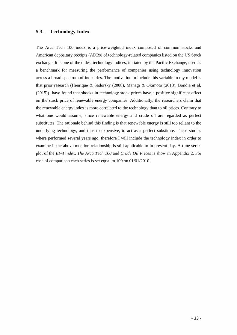
- 33 -

5.3. Technology Index

The Arca Tech 100 index is a price-weighted index composed of common stocks and

American depositary receipts (ADRs) of technology-related companies listed on the US Stock

exchange. It is one of the oldest technology indices, initiated by the Pacific Exchange, used as

a benchmark for measuring the performance of companies using technology innovation

across a broad spectrum of industries. The motivation to include this variable in my model is

that prior research (Henrique & Sadorsky (2008), Managi & Okimoto (2013), Bondia et al.

(2015)) have found that shocks in technology stock prices have a positive significant effect

on the stock price of renewable energy companies. Additionally, the researchers claim that

the renewable energy index is more correlated to the technology than to oil prices. Contrary to

what one would assume, since renewable energy and crude oil are regarded as perfect

substitutes. The rationale behind this finding is that renewable energy is still too reliant to the

underlying technology, and thus to expensive, to act as a perfect substitute. These studies

where performed several years ago, therefore I will include the technology index in order to

examine if the above mention relationship is still applicable to in present day. A time series

plot of the EF-I index, The Arca Tech 100 and Crude Oil Prices is show in Appendix 2. For

ease of comparison each series is set equal to 100 on 01/01/2010.

- 34 -

Figure 2: Graphical view of the variables in levels and first-differences

40

50

60

70

80

90

100

2010 2011 2012 2013 2014 2015 2016

EF-I Index

-6

-4

-2

0

2

4

6

2010 2011 2012 2013 2014 2015 2016

D_EF_I_INDEX

20

40

60

80

100

120

140

2010 2011 2012 2013 2014 2015 2016

Crude Oil Price

-10

-8

-6

-4

-2

0

2

4

6

2010 2011 2012 2013 2014 2015 2016

D_CRUDE_OIL_PRICE

800

1,000

1,200

1,400

1,600

1,800

2,000

2,200

2010 2011 2012 2013 2014 2015 2016

Arca Tech 100

-100

-80

-60

-40

-20

0

20

40

60

80

2010 2011 2012 2013 2014 2015 2016

D_ARCA_TECH_100

- 35 -

6 Empirical Results

In this section I will elaborate on the empirical results obtained by my analysis, using the

methodology that I explained in section 4. Before examining the hypotheses mentioned

above, in this section the statistical validity of the model is tested. The reason to test the

statistical validity of the model is to determine which models to use in my analysis and to

examine if I have to make adjustments to my model in order to make sure it produces robust

results. I perform this examination prior to analysis of the relationship between oil prices and

renewable energy stock performance, because using the wrong model will result in

misleading and incorrect results. Throughout this section I will present the results of the full

EF-I index first and the results of the EF-I of the sub-divisions and sub-industries afterwards.

6.1. Stationarity

In section 5 there is a graphical illustration of how the EF-I index, the crude oil price and the

Arca Tech 100 develop form Q1 in 2010 up to and including Q4 of 2016. A visual

examination of the graphs results that one would conclude that the time series contain a unit

root. This is in accordance with what I expected, because stock prices usually contain unit

roots. During the sample period, two of the three indices have only been subject to growth

with occasional short setbacks. The decision of my sample period that I use, is to only use

data of after the financial crisis, in order to take out all influencing factors of the crisis. The

reason to use this practice was to yield results that only apply to periods without significant

difficulty in the stock market. When analysing the oil price, the price of crude oil is stable

during the sample period until the end of 2014 that is followed by a major decline in the oil

price. However visual analysis of the graph is not conclusive in determining if the time series

contains a unit root. I have to use the previously mentioned Augmented Dickey-Fuller test, if

I want to be conclusive about the stationarity.

In this paper I use a 5% significant level, since most similar studies use the same level to

examine their results. Additionally, the null hypothesis in all tests are the same, namely if the

variable is non-stationary. Figure 2 shows the graphical development of the variables and

Table 3 shows the test results for all the variables. In the tables 3,4 and 5 I will use the Δ

symbol in order to indicate the first-difference of a particular variable. The first variable that I

am going to analyse using the “augmented Dickey-Fuller test” is Oil Price. The ADF test

indicates that with a probability of 0.7963 being greater than the 0.05 significant level, that

the null hypothesis (non-stationarity) cannot be rejected. This would mean that the variable

- 36 -

Oil Price could be non-stationary and thus cannot be used to analyse the relationship between

oil prices and renewable energy companies. Therefore, I performed the same test using the

first difference of the variable, in order to make the variable stationary which is denoted as

∆Oil Price. The outcome of the test shows that the null hypothesis can be rejected, and thus

the variable ∆Oil Price is regarded as stationary and can be used in the analysis. I performed

the same routine for the variable EF I Index, the outcome of the level values shows a

probability of 0.5434 which is greater than the previously mentioned 5% and thus can the null

hypothesis not be rejected. Subsequently, I took the first difference of the variable, which is

denoted as ∆EF I Index, and performed the same test again. The second outcome resulted in a

probability of 0.0000, therefore rejecting the null hypothesis. The same tests is performed for

the variable Arca Tech 100, resulting in an outcome of 0.2268 as p-value on in levels thus I

could not reject the null hypothesis. However, after differencing the variable denoted as

∆Arca Tech 100, the outcome is 0.000. Therefore rejecting the null hypothesis in first-

differences meaning that the variable is stationary. Thus it can be concluded that all variables

in the full EF-I Index model are integrated in the order of 1 . The results are shown in

the table below:

Table 3: Augmented Dickey-Fuller test on the full model

Variable: Exogenous variable: Lag length: Test statistic: Probability:

EF-I Index Constant, Linear Trend 4 -2.102779 0,5434

Oil Price Constant 1 -0.875625 0.7963

Arca Tech 100 Constant, Linear Trend 3 -2.724080 0.2268

ΔEF-I Index None 3 -23.49011 0.0000

ΔOil Price None 0 -39.61496 0.0000

ΔArca Tech 100 None 2 -26.48010 0.0000

Notes: *p < 0.10, **p < 0.05, ***p < 0.01, Lag length criteria by AIC, ∆ represents the first difference of the

variable

In order to examine my second hypothesis regarding the companies that are operating in

different renewable energy sectors, I performed the same unit root tests. Almost all the

variables contain a unit root, namely

and . Accordingly, for these variables I have included the

differenced values and tested these for an unit root. None of the differenced variables contain

a unit root and thus can be concluded that these variables are integrated in the order of 1,

which can be noted as 1 . The remaining variable is not subject to the unit

root in its level values, therefore I did not include the differenced variable.

- 37 -

Table 4: Augmented Dickey-Fuller test on the sub-industries

Variable: Exogenous variable: Lag length: Test statistic: Probability:

Constant, Linear Trend 4 -1.752782 0.7272

Constant 1 -2.459794 0.1257

Constant 0 -2.104479 0.2430

Constant 4 -1.827489 0.3673

Constant 5 -2.491206 0.1177

Constant, Linear Trend 1 -2.950287 0.1469

Constant, Linear Trend 0 -3.692976 0.0230**

None 3 -23.81472 0.0000***

None 0 -44.28747 0.0001***

None 0 -43.26544 0.0001***

None 3 -23.73761 0.0000***

None 4 -21.23717 0.0000***

None 0 -44.60497 0.0001***

Notes: *p < 0.10, **p < 0.05, ***p < 0.01, Lag length criteria by AIC, ∆ represents the first difference of the

variable

The last part of this section is dedicated to the ADF-test analysis of each of the supply chain

divisions in which the renewable energy companies operate. I perform the unit root test for

the remaining variables in a similar fashion as the previous variables. The outcomes show that

all the variables are integrated in the first order , except . Therefore,

I only included the differenced values of the other variables and tested the differenced

variable for a unit root. All the remaining variables are not subject to a unit root, thus they can

be used in my model. In table 5, all the outcomes of the ADF-test are presented.

- 38 -

Table 5: Augmented Dickey-Fuller test on the sub-division

Variable: Exogenous variable: Lag Length: Test statistic: Probability:

Constant, Linear Trend 0 -2.672891 0.2481

Contant 0 -1.279878 0.6410

Contant 0 -2.157622 0.2223

Constant, Linear Trend 4 -1.853415 0.6781

Constant, Linear Trend 1 -2.949231 0.1472

Constant, Linear Trend 0 -4.096031 0.0064**

None 0 -43.13689 0.0001***

None 0 -42.90890 0.0001***

None 0 -43.36316 0.0001***

None 3 -23.79583 0.0000***

None 0 -45.27204 0.0001***

Notes: *p < 0.10, **p < 0.05, ***p < 0.01, Lag length criteria by AIC, ∆ represents the first difference of the

variable

In table 6, an overview of the outcomes of the ADF-test to identify the order integration of all

the variables examined in this paper is included for the ease of comparison.

Table 6: Overview outcomes Augmented Dickey-Fuller test

Variable: Integration order: Lag length:

EF-I_Index I(1) 4

Oil_Price I(1) 1

Arca_Tech_100 I(1) 3

I(1) 4

I(1) 1

I(1) 0

I(1) 4

I(1) 5

I(1) 1

I(0) 0

I(1) 0

I(1) 0

I(1) 0

I(1) 4

I(1) 1

I(0) 0

- 39 -

6.2. Co-integration

In section 4.3., I explained the matter of co-integration, it occurs in a model when two or

more variables share a common stochastic drift resulting that their long-term fluctuations and

trend are subject to the same movements. Since renewable energy and crude oil are assumed

to be substitutes, one would expect that these variables share a common stochastic drift. In

general commodity prices show integration of order 1, l(1), or non-stationary. This stochastic

drift is examined in this section.

I am interested in the effect of the variables ∆Oil Price and ∆Arca Tech 100 on the renewable

energy market. Additionally, I use the same two variables to analyse the effect on the created

sub-divisions and sub-industries of the EF-I index. In accordance with the Engle-Granger

method I run the level regression using Least Squares (OLS) and capture the residuals.

The results of the Engle-Granger test show that the null hypothesis cannot be rejected since

the probability is greater than the 5% significance level used in this paper. The t-statistic for

this ADF test for the residuals of the variables Oil Price, EF I Index and Arca Tech 100

outcome is -2.524760 with the corresponding p-value of 0.1097. However, since the ADF test

is now used to test for co-integration in the residual term, the standard p-value is invalid.

Therefore, I use the t-statistic value -2.524760 and compare it against the set of critical values

provided by Davidson & Mackinnen (1993). This table shows that when using 3 variables and

a constant in the unit root test, the critical values of -3.34 at a significance level of 5% has to

be used. Since my t-statistic -2.524760 is much greater than these values the I fail to reject

the null hypothesis at a significance level of 5%. The means that there is a unit root in the

series and that the residual term is not stationary, thus there is no cointegration among the

variables.

I performed the same routine for all the sub-divisions and sub-industries, the outcomes of the

Engle-Granger tests are shown in table 7. All the t-statistic values are larger than the

corresponding critical values provided by Davidson & Mackinnen. Therefore, I can conclude

that there is a unit root in the series and the residual terms are not stationary. As for the

and , they are not included in the analysis, because testing for

cointegration in models that contain variables that are and is useless.

- 40 -

Table 7: Overview outcomes Engle-Granger test

Variable: Residual: Lags

Critical value: T-statistic:

Constant 3 -3.74 -2.524760**

Constant, Linear Trend 1 -4.12 -3.968149**

None 1 -3.74 -3.418361**

Constant, Linear Trend 1 -4.12 -3.968149**

Constant, Linear Trend 13 -4.12 -3.335915**

Constant, Linear Trend 5 -4.12 -3.402028**

Constant 1 -3.74 -3.290520**

Constant, Linear Trend 10 -4.12 -2.551226**

Constant 1 -3.74 -2.871531**

Constant 1 -3.74 -3.040792**

Constant 3 -3.74 -2.313953**

Constant, Linear Trend 1 -4.12 -3.582737**

Notes: *p < 0.10, **p < 0.05, ***p < 0.01, Lag length criteria by AIC,

6.3. Lag selection and Stability

In section 4.4., I elaborated on the method of appropriate lag selection and the tests that I will

use in order to determine the optimal lag length of my model. The trade-off that as to be made

while determining the optimal number of lags in a VAR model, is when the used lag length is

too short the model fails to capture the time series’ dynamics and when the lag length is too

long every extra added lag makes the estimation of the coefficients more complex and thus

vulnerable to inaccuracies.

It could be that the selection criterion outcomes show varying optimal lag lengths, in such

case I have to make a deliberate choice in selecting the best possible lag length. This must be

done carefully since the cointegration among the variables is directly dependent on the chosen

lag length (Emerson, 2007). The AIC and SC tests show contradicting results for the VAR

using the full EF-I Index, as can be seen in Table 8. When the outcomes of the variables,

result in conflicting values I have chosen to use the AIC value in accordance with similar

studies. Additionally, for all the sub-divisions and sub-industries I determined the optimal lag

length by analysing the AIC and SC values of the VAR models with ∆Oil Price, ∆Arca Tech

100 and one of the ∆EF-I Indices. Together with the optimal lag length of the VAR model

with the full EF-I variable, the lag lengths of VAR models with the sub-divisions and sub-

industries are shown in the table 8.

- 41 -

Table 8: Overview outcomes Information Criteria

Variable: LR FPE AIC* SC HQ

2 2 2 0 1

1 1 1 0 0

3 1 1 0 0

0 0 0 0 0

3 3 3 0 0

7 3 3 0 0

3 1 1 0 0

1 1 1 1 1

6 2 2 0 0

3 2 2 0 0

3 3 3 0 0

1 1 1 0 1

1 1 1 1 1

1 1 1 1 1

The autocorrelation LM test shows that a lag selection of 2 is sufficient, the null hypothesis of

no serial correlation can be rejected only at a lag length of 2 for the model with variable EF-I.

Additionally, in the same model residual autocorrelation is tested using Portmanteau test and

it showed that the lag length of 2 was sufficient and no residual autocorrelation was found in

the time series. Lastly, the model is tested for normality and heteroskedasicity, output shows

that all of the necessary assumptions regarding an statistically valid model are not violated.

In order to examine the stability, I use the graphs of the Inverse Roots of the AR

Characteristic Polynomial. All values of the Inverse Roots are inside the unit circle as can be

seen in Figure 3. This is important because if the VAR(2) is not stable, certain outcomes of

the model would not be valid. However that is not applicable to our variables. If the figure

would have shown values outside the unit circle, it would mean that one of variables is

integrated in the first order. Since we already removed that option in de first segment of this

section is was not applicable to my situation. Additionally, if the figure would show values

outside the unit circle, co-integration within the variables could exist and it would be better to

analyse the variables in the context a Vector Error Correction Model (VECM).

- 42 -

Figure 2: Stability EF-I Variables (Inverse Roots of AR Characteristic Polynomial)

-1.5

-1.0

-0.5

0.0

0.5

1.0

1.5

-1.5 -1.0 -0.5 0.0 0.5 1.0 1.5

Inverse Roots of AR Characteristic Polynomial

After performing all the preceding tests mentioned above, the VAR(2) model is noted as:

All the tests mentioned in this section, are performed for the remaining variables and the

outcomes do not violate the requirements necessary to make a statistically valid model. When

they did, in some rare cases, the correct actions have been taken to make the model statically

valid.

- 43 -

6.4. Granger Causality

The Granger causality test is used to examine the causality between two variables in a time

series. The test is used to analyse if the lagged value of one of the variables has explanatory

power over the non-lagged values of one of the other values. In order words if that is the

cause, A variable X Granger-causes Y if Y can be better predicted using the lagged values of

both X and Y than it can using the lagged value of Y alone. The null hypothesis in Granger

Causality tests assume there is no causality from one variable to another. Hence if the null

hypothesis is rejected at a significance level of 5%, means that one variable is granger causal

the other variable.

Table 9: Overview outcomes Pairwise Granger Causality test

Null hypothesis: Lags Obs. F-Statistics Probability

∆Oil Price does not Granger Cause ∆EF-I Index 2 1823 4.40809 0.0083**

∆EF-I Index does not Granger Cause ∆Oil Price 0.90833 0.4034

∆Arca Tech 10 does not Granger Cause ∆EF-I Index 2 1823 10.6054 3.E-05***

∆EF-I Index does not Granger Cause ∆Arca Tech 10 018478 0.8313

∆Arca Tech 10 does not Granger Cause ∆Oil Price 2 1823 0.92727 0.3958

∆Oil Price does not Granger Cause ∆Arca Tech 10 3.78347 0.0229

Notes: *p < 0.10, **p < 0.05, ***p < 0.01

As shown in table 9, the null hypothesis indicates that one variable is not granger causal for

another variable is rejected for ∆Oil Price and ∆Arca Tech 10 in terms of ∆EF-I Indices. This

outcome means that the causality from the EF-I Index to the oil price and technology index is

significant. In other words, the oil price and the technology index are one of the reasons that

causes the volatility in the EF-I index. However, the outcomes show that the inverse causality

is not valid for ∆EF-I Indices to ∆Oil Price and ∆Arca Tech 10. Therefore, the crude oil price

and the technology index are drivers of the EF-I index, but not the other way around.

The granger causality test is performed in the same manner for the sub-divisions and sub-

industries, all the outcomes can be seen in Appendix 3. In general, the sub-divisions and sub-

industries show similar results as for the full EF-I database, with some specific divisions

showing varying results.

- 44 -

6.5. Impulse Response Functions

The impulse response functions are shocks to the VAR(2) system. In other words, they

identify the response of a certain variable to an exogenous shock on the whole process over

time. Thus, one can detect the dynamic relationships over time, and therefore I am able to

analyse the effect of fluctuations in oil prices to the stock performance of companies active in

renewable energy sector. This is the first hypothesis I will examine, in this paper. An

exogenous one standard deviation shock in the variable ∆Crude Oil and in ∆Arca Tech 100

using a Cholesky distribution with a 95% confidence interval is shown in figure 4.

Figure 3: Impulse Response of the EF-I Index to Crude Oil prices and Arca Tech 100

The outcome of the impulse response function shows that a shock in the oil price results in an

upward movement in the EF-I index on the second and third day after the shock. The result

of the same shock for ∆Arca Tech 100 is reflected in large upward movement in the second

day followed by a small and almost neglectable negative movement on the fourth day. This

finding is in accordance with the studies in the literature review, since the overall consensus

of the papers was that the renewable energy is correlated to the crude oil price however more

correlated to technology companies. The rationale behind this finding is that renewable

energy companies are still too dependent on the underlying technology to be regarded as a

perfect substitute for crude oil. Consequently, this also the answer to my first hypothesis.

The next hypothesis that is analysed is defined as: The effect of fluctuations in oil prices on

the stock performance of renewable energy companies is dependent on the position of the

renewable energy company in the supply chain. Therefore, I examined the companies active

in certain areas of the supply chain individually. Companies involving the R&D and

manufacturing sector of renewable energy show an upward movement after a shock in the oil

price, not within the 95% confidence interval. Nevertheless, the shock in the technology index

- 45 -

is positive as well but does fall within in the confidence interval followed by a small negative

movement, very similar to model with the full EF-I sample. The reassembly part of the

renewable energy supply chain reacts with a positive movement after an impulse in the oil

price but not significant. The same movement can be identified for the second impulse

however significant followed by a small negative movement that is not significant. The

services industry show for both shocks an upward movement, that is significant for the

technology shock however not for the oil price shock. A non-significant positive upward

moment can be detected for both impulses, for companies that generate renewable energy.

Finally, companies that transport energy to the final user show negative movements after the

two shocks. The of the movements after an impulse in the crude oil price is significant, but

the movement after the shock in the technology sector is not. Hence it is hard to make

conclusive assumptions about this industry. Especially because they act in an remarkable

different manner compared to the other models and their effect is lasting, this probably due to

the fact that the level values are used. Concluding, when examining the companies on a

supply chain level, they show similar results as the full sample except companies that operate

in the transportation sector. All the impulse response functions are included in Appendix 6.

One could argue that certain renewable energy industries are more mature than others and are

therefore more correlated with crude oil, since generating energy using a more mature

technology is less costly. Since the generation of energy is less costly it could possibly act as

a substitute for crude oil. Therefore, I examined the effect of a one standard deviation in the

crude oil price on the sub-industries individually, using the same methodology as mentioned

in section 4 en 6 explained for the full EF-I index. All the outcomes are included in Appendix

6. The first sub-industry that I examine is biomass, when put subject to the same one standard

deviation impulse of oil price and technology index. shows exactly the same, but

less extreme movements as for the full EF-I index. As for the companies that operate

wave/ocean energy industry denoted as EF-Iwave, the same test creates a similar small upward

movement for both shocks however less extreme. Companies active in the photovoltaic

energy industry, show even smaller upward movements, these movements are almost

neglectable. The shocks could also results in a small negative movement, when taking in

account the 95% confidence interval. Solar energy shows in the beginning an upward

movement, followed by a negative movement in the days after. It is difficult to make definite

conclusions about the shocks to companies active in solar energy, since they show that within

the confidence interval the shocks could be positive as well as negative. The geothermal

industry acts in a similar fashion as the solar industry in terms of the shock in oil price,

however regarding the technology shock it reacts in the complete opposite way. Companies

active in the wind energy industry respond in the same manner as companies active in the

- 46 -

photovoltaic energy and wave industry. Hence, they show upward movements for both

impulses however they are small movements. Finally, the hydro industry shows an non-

significant upward movement after a shock in the oil price and they do not respond to an

impulse in the technology index. Therefore, it is difficult to be conclusive about these

companies due to similar reasons as the companies active in the transportation sector.

Concluding, the full EF-I sample shows a stronger movement after the shock in the

technology index than to crude oil price fluctuations. However when examining the sub-

industries individually this effect is not present. The majority of the sub-industries show a

stronger correlation with oil prices than to the technology index. Contrary to the sub-

industries, in general the sub-division show similar movements as the movement of the full

EF-I Index model.

Table 10: Overview outcomes Impulse Response Functions

Oil Price Arca Tech 100

Variable: Short

Term:

Long

Term:

Short

Term:

Long

Term:

+* 0* +* -*

+* 0* +* -*

+* 0* +* -*

+ 0* + 0*

+ - + -

+ - - +

+ 0* + 0*

+ + 0 0

+ 0 +* -

+ 0 +* -

+ 0 +* -

+ 0 +* 0

+ 0 + 0

- - -* -*

The majority of the variables show a upward movement in the first days, some are within the

95% confidence interval and some are not, continued by a diminishing effect that flows back

to a constant of zero. The impulse response functions show that seven of the fourteen

variables move in this similar fashion.

- 47 -

The most striking differences in all the sub-industries and sub-division is the impulse

response of the geothermal renewable energy industry. The companies within that industry

show an downward movement in the first days after a shock in the technology index and

some small downward movements in de days after a shock in the oil price. The geothermal

renewable energy industry is, singular in that effect and thus reacts remarkably different to

the impulses than all the other companies. The impulse response functions of the mentioned

industry is shown in figure 4. Companies that operate in the solar industry react similar to

fluctuations in oil prices, however they react completely opposite to impulses in technology

index. This can be seen in figure 5.

Figure 4: Impulse Response of the EF-I geothermal to Crude Oil prices and Arca Tech 100

Figure 5: Impulse Response of the EF-I solar to Crude Oil prices and Arca Tech 100

The last two divisions that I would like to highlight are the companies that are operating the

in hydro/ocean industry and the companies that are occupied with the transportation of

renewable energy to the end-user. These variables were not , therefore I used the level

values of these variables in my model. As a result, they show significantly different impulse

response functions, as can be seen in the figures 6 and 7. Companies that are active in the

hydro industry show an upward movement from the second day onward, while a fluctuation

- 48 -

in the technology index has no significant effect on the companies. The companies that are

involved with the transportation of renewable energy to the end-user react show a negative

movement for both shocks. Figure 7 shows that de downward movement after a shock in oil

price is not significant, but the impulse in the technology index is. All the impulse response

functions that I are not highlighted individually are shown in Appendix 6.

Figure 6: Impulse Response of the EF-I hydro/ocean to Crude Oil prices and Arca Tech 100

Figure 7: Impulse Response of the EF-I transportation to Crude Oil prices and Arca Tech 100

Overall, one can conclude that the stock price of renewable energy is positively correlated to

the oil price. However, since most of the underlying technology is still evolving I find that the

renewable energy companies in my sample period are more effected by fluctuations in the

technology index. This dynamic is visible when analysing the sub-industries individually, one

can see that the more mature industries are more correlated to the oil price and the more

juvenile industries are more correlated to the technology index. When examining the

companies on a supply chain level, all the indices are more affected by an impulse on the

technology index then to a shock in the oil price.

- 49 -

7 Discussion

In this section, the implications of my findings and an general overview will be given in the

first section. In the second section, I will elaborate on the limitations of my paper. Finally in

section 7.3 suggestions for further research are disclosed.

7.1. Conclusion

In this paper I set out to improve the investment decisions involving renewable energy

companies, more specifically the dynamic interactions between renewable energy and crude

oil. In order to analyse this relationship, I use a vector auto regression model with daily data

obtained from Datastream using a sample period of Q1 2010 up to and including Q4 2016.

The renewable energy data is comprised of a self-made capitalization weighted float adjusted

equity index of the companies that are included in the EF-I database, calculated using stock

prices and market values. As for the crude oil price, I used the average of the WTI crude oil

price and the Brent blend crude oil price. Finally for the technology index, I have selected the

Arca Tech 100 following many other similar studies.

The aim of this paper is to provide more information about the dynamics of the renewable

energy industry and how it reacts on its substitute crude oil and the underlying technology.

The rationale behind this is that if one would assume that crude oil is a perfect substitute of

renewable energy then they should be positively correlated. However, it could also be that

the renewable energy is still too dependent on the underlying technology to act as a perfect

substitute for crude oil. I find using the impulse response functions that the more mature

technologies such as wind and wave powered energy, are more influenced by the oil price

then less mature technologies as geothermal and photovoltaics. However, more juvenile

industries such as biomass show that more correlation with the underlying technology. When

analysing the sub-industries, the effect of the two shocks show varying results among the

industries, whereas on supply chain level each division reacts more on technology shocks

than to fluctuations in oil prices. Concluding, renewable energy companies are influenced by

the fluctuations in crude oil price, however the effect is larger regarding the underlying

technology, this is something that investors have to keep in mind while making investment

decisions.

- 50 -

7.2. Limitations

One of the limitations of this paper could be the aspect of human error in creating a database

and indices. I have full confidence that the data that I use in my model is reliable and well

thought out. However, it could always be that when someone else made these indices they

would have made different decisions in terms of selection of the data. Additionally, one of the

largest factors in changes in the renewable energy stock prices is explained by changes in the

policy of renewable energy. The reason that I did not include this factor in my model, is that I

want to single out and analyse the oil price and technology index factors. This factor,

renewable energy policy, is not included in my paper and could be incorporated while further

research will be done.

7.3. Further research

In my opinion, further research with more focus on geographical regions can be performed.

One could argue that within countries where renewable energy already generally is more

accepted as a source of energy, it acts more as a perfect substitute for crude oil. Furthermore,

as the research studies countries individually, the split can be made between oil importing and

exporting countries. In order to, single out the relationship of crude oil and renewable energy,

on a country level one could control for macroeconomic factors. Additionally, renewable

energy technology is continuously developing. Therefore, in the future when using recent data

one could obtain significantly different results. Since, by the usage of a more developed

technology, the production cost of renewable energy will be reduced drastically, this will

ensure that renewable energy can truly act as a substitute for crude oil. Lastly, I have used

daily data to examine the relationship, one could use a different data interval in order to find

other dynamic interactions.

- 51 -

8 References

Akaike, H. (1976). Canonical correlation analysis of time series and the use of an information

criterion. Mathematics in Science and Engineering, 126, 27-96.

Ben-David, I., Graham, J. R., & Harvey, C. R. (2010). Managerial

miscalibration (No.w16215). National Bureau of Economic Research.

Bondia, R., Ghosh, S., & Kanjilal, K. (2016). International crude oil prices and the stock

prices of clean energy and technology companies: Evidence from non-linear

cointegration tests with unknown structural breaks. Energy, 101, 558-565.

Brooks, C. (2008). Introductory Econometrics Finance. New York: Cambridge University

Press.

Büyüksahin, B., Lee, T. K., Moser, J. T., & Robe, M. A. (2013). Physical markets, paper

markets and the WTI-Brent spread. The Energy Journal, 34(3), 129.

Chen, W., Huang, Z., & Yi, Y. (2015). Is there a structural change in the persistence of WTI–

Brent oil price spreads in the post-2010 period?. Economic Modelling, 50, 64-71.

De Bondt, W. F., & Thaler, R. (1985). Does the stock market overreact?. The Journal of

finance, 40(3), 793-805.

Engle, R. F., & Granger, C. W. (1987). Co-integration and error correction: representation,

estimation, and testing. Econometrica: journal of the Econometric Society, 251-276.

Emerson, J. (2007). Cointegration analysis and the choice of lag length. Applied economics

letters, 14(12):881-885

Fama, E. F. (1970). Efficient capital markets: A review of theory and empirical work. The

journal of Finance, 25(2), 383-417.

Granger, C. W. (1969). Investigating causal relations by econometric models and cross-

spectral methods. Econometrica: Journal of the Econometric Society, 424-438.

- 52 -

Granger, C. W. (1980). Testing for causality: a personal viewpoint. Journal of Economic

Dynamics and control, 2, 329-352.

Grossman, S. J., & Stiglitz, J. E. (1980). On the impossibility of informationally efficient

markets. The American economic review, 70(3), 393-408.

Grøm, H. A. (2013). The relationship between renewable energy assets and crude oil

prices (Doctoral dissertation, Norwegian School of Economics).

Henriques, I., & Sadorsky, P. (2008). Oil prices and the stock prices of alternative energy

companies. Energy Economics, 30(3), 998-1010.

Huang, A. Y., Cheng, C. M., Hu, W. C., & Chen, C. C. (2011). Relationship between crude

oil prices and stock prices of alternative energy companies with recent

evidence. Economics Bulletin, 31(3), 2434-2443.

Inchauspe, J., Ripple, R. D., & Trück, S. (2015). The dynamics of returns on renewable

energy companies: A state-space approach. Energy Economics,48, 325-335.

International Energy Agency. (2015). World Energy Outlook, IEA, Paris.

James, B. B. T. K. L., & Robe, T. M. M. A. (2012). Physical Market Conditions, Paper

Market Activity, and the WTI-Brent Spread.

Kumar, S., Managi, S., & Matsuda, A. (2012). Stock prices of clean energy firms, oil and

carbon markets: A vector autoregressive analysis. Energy Economics, 34(1), 215-226.

Managi, S., & Okimoto, T. (2013). Does the price of oil interact with clean energy prices in

the stock market?. Japan and the World Economy, 27, 1-9.

Marchall, A. (1890). Principles of economics, Macmillan and Co.

Malkiel, B. G., & Fama, E. F. (1970). Efficient capital markets: A review of theory and

empirical work. The journal of Finance, 25(2), 383-417.

Malmendier, U., & Tate, G. (2005). CEO overconfidence and corporate investment. The

journal of finance, 60(6), 2661-2700.

- 53 -

Omri, A., & Nguyen, D. K. (2014). On the determinants of renewable energy consumption:

International evidence. Energy, 72, 554-560.

Omri, A., Daly, S., & Nguyen, D. K. (2015). A robust analysis of the relationship between

renewable energy consumption and its main drivers. Applied Economics, 47(28),

2913-2923.

Phillips, P. C. (1986). Understanding spurious regressions in econometrics. Journal of

econometrics, 33(3), 311-340.

Sadorsky, P. (2009). Renewable energy consumption, CO 2 emissions and oil prices in the G7

countries. Energy Economics, 31(3), 456-462.

Sadorsky, P. (2011). Modeling renewable energy consumption for a greener global economy.

INTECH Open Access Publisher.

Sadorsky, P. (2012a). Correlations and volatility spillovers between oil prices and the stock

prices of clean energy and technology companies. Energy Economics, 34(1), 248-

255.

Sadorsky, P. (2012b). Modelling renewable energy company risk. Energy Policy, 40, 39-48.

Sarkar, N., & Brooks, C. (2003). Introductory Econometrics for Finance. Cambridge

University Press, United Kingdom

Sims, C. A. (1980). Macroeconomics and reality. Econometrica: Journal of the Econometric

Society, 1-48.

Schmitz, A. (2009). Effect of oil prices on returns to alternative energy investments (Doctoral

dissertation, Georgia Institute of Technology).

Tversky, A., & Kahneman, D. (1991). Loss aversion in riskless choice: A reference-

dependent model. The quarterly journal of economics, 1039-1061.

Reboredo, J. C. (2015). Is there dependence and systemic risk between oil and renewable

energy stock prices?. Energy Economics, 48, 32-45.

- 54 -

Rockström, J., Steffen, W. L., Noone, K., Persson, Å., Chapin III, F. S., Lambin, E. &

Nykvist, B. (2009). Planetary boundaries: exploring the safe operating space for

humanity.

Rukavishnikova, A., & Baars, N. (2014). The Impact of Oil Price Fluctuations on Stock

Performance of Clean Energy Companies: A global study on a corporate level.

Schwarz, G. (1978). Estimating the dimension of a model. The annals of statistics, 6(2), 461-

464.

United Nations. (1995). Kyoto Protocol to The United Nations Framework Convention on

Climate Change. United Nations.

Varian, H. R. (2014). Intermediate Microeconomics: A Modern Approach: Ninth

International Student Edition. WW Norton & Company.

Wen, X., Guo, Y., Wei, Y., & Huang, D. (2014). How do the stock prices of new energy and

fossil fuel companies correlate? Evidence from China. Energy Economics, 41, 63-75.

9 Appendix

Appendix 1: Indexed graphical view of the EF-I index, MSCI world index and S&P 500 index

- 55 -

Appendix 2: Indexed graphical view of the EF-I index, Oil price and Arca Tech 100

Appendix 3a: Stability EF-I (Inverse Roots of AR Characteristic Polynomial)

-1.5

-1.0

-0.5

0.0

0.5

1.0

1.5

-1.5 -1.0 -0.5 0.0 0.5 1.0 1.5

Inverse Roots of AR Characteristic Polynomial

- 56 -

Appendix 3b: Stability EF-Ibio (Inverse Roots of AR Characteristic Polynomial)

-1.5

-1.0

-0.5

0.0

0.5

1.0

1.5

-1.5 -1.0 -0.5 0.0 0.5 1.0 1.5

Inverse Roots of AR Characteristic Polynomial

Appendix 3c: Stability EF-Iwave (Inverse Roots of AR Characteristic Polynomial)

-1.5

-1.0

-0.5

0.0

0.5

1.0

1.5

-1.5 -1.0 -0.5 0.0 0.5 1.0 1.5

Inverse Roots of AR Characteristic Polynomial

Appendix 3d: Stability EF-Iphoto (Inverse Roots of AR Characteristic Polynomial)

-1.5

-1.0

-0.5

0.0

0.5

1.0

1.5

-1.5 -1.0 -0.5 0.0 0.5 1.0 1.5

Inverse Roots of AR Characteristic Polynomial

- 57 -

Appendix 3e: Stability EF-Isolar (Inverse Roots of AR Characteristic Polynomial)

-1.5

-1.0

-0.5

0.0

0.5

1.0

1.5

-1.5 -1.0 -0.5 0.0 0.5 1.0 1.5

Inverse Roots of AR Characteristic Polynomial

Appendix 3f: Stability EF-Igeothermal (Inverse Roots of AR Characteristic Polynomial)

-1.5

-1.0

-0.5

0.0

0.5

1.0

1.5

-1.5 -1.0 -0.5 0.0 0.5 1.0 1.5

Inverse Roots of AR Characteristic Polynomial

Appendix 3g: Stability EF-Iwind (Inverse Roots of AR Characteristic Polynomial)

-1.5

-1.0

-0.5

0.0

0.5

1.0

1.5

-1.5 -1.0 -0.5 0.0 0.5 1.0 1.5

Inverse Roots of AR Characteristic Polynomial

- 58 -

Appendix 3h: Stability EF-Ihydro (Inverse Roots of AR Characteristic Polynomial)

-1.5

-1.0

-0.5

0.0

0.5

1.0

1.5

-1.5 -1.0 -0.5 0.0 0.5 1.0 1.5

Inverse Roots of AR Characteristic Polynomial

Appendix 3i: Stability EF-IR&D (Inverse Roots of AR Characteristic Polynomial)

-1.5

-1.0

-0.5

0.0

0.5

1.0

1.5

-1.5 -1.0 -0.5 0.0 0.5 1.0 1.5

Inverse Roots of AR Characteristic Polynomial

Appendix 3j: Stability EF-Imanufacturing (Inverse Roots of AR Characteristic Polynomial)

-1.5

-1.0

-0.5

0.0

0.5

1.0

1.5

-1.5 -1.0 -0.5 0.0 0.5 1.0 1.5

Inverse Roots of AR Characteristic Polynomial

- 59 -

Appendix 3k: Stability EF-IReassembly (Inverse Roots of AR Characteristic Polynomial)

-1.5

-1.0

-0.5

0.0

0.5

1.0

1.5

-1.5 -1.0 -0.5 0.0 0.5 1.0 1.5

Inverse Roots of AR Characteristic Polynomial

Appendix 3l: Stability EF-IServices (Inverse Roots of AR Characteristic Polynomial)

-1.5

-1.0

-0.5

0.0

0.5

1.0

1.5

-1.5 -1.0 -0.5 0.0 0.5 1.0 1.5

Inverse Roots of AR Characteristic Polynomial

Appendix 3m: Stability EF-Igenerating (Inverse Roots of AR Characteristic Polynomial)

-1.5

-1.0

-0.5

0.0

0.5

1.0

1.5

-1.5 -1.0 -0.5 0.0 0.5 1.0 1.5

Inverse Roots of AR Characteristic Polynomial

- 60 -

Appendix 3n: Stability EF-ITransportation (Inverse Roots of AR Characteristic Polynomial)

-1.5

-1.0

-0.5

0.0

0.5

1.0

1.5

-1.5 -1.0 -0.5 0.0 0.5 1.0 1.5

Inverse Roots of AR Characteristic Polynomial

Appendix 4a: Pairwise Granger Tests EF-Ibio

Appendix 4b: Pairwise Granger Tests EF-Iwave

- 61 -

Appendix 4c: Pairwise Granger Tests EF-Iphoto

Appendix 4d: Pairwise Granger Tests EF-Isolar

Appendix 4e: Pairwise Granger Tests EF-Igeothermal

- 62 -

Appendix 4f: Pairwise Granger Tests EF-Iwind

Appendix 4g: Pairwise Granger Tests EF-Ihydro

Appendix 4h: Pairwise Granger Tests EF-IR&D

- 63 -

Appendix 4i: Pairwise Granger Tests EF-Imanufacturing

Appendix 4j: Pairwise Granger Tests EF-IReassembly

Appendix 4k: Pairwise Granger Tests EF-Iservices

- 64 -

Appendix 4l: Pairwise Granger Tests EF-Igenerating

Appendix 4m: Pairwise Granger Tests EF-ITransportation

- 65 -

Appendix 5: Vector Autoregression Estimates EF-I

Vector Autoregression Estimates

Date: 03/02/17 Time: 15:25

Sample (adjusted): 1/06/2010 12/30/2016

Included observations: 1823 after adjustments

Standard errors in ( ) & t-statistics in [ ] D_EF_I_INDEX D_OILP D_PACXTEC D_EF_I_INDEX(-1) -0.096156 -0.077618 -0.069650

(0.02839) (0.03949) (0.49462)

[-3.38671] [-1.96554] [-0.14081]

D_EF_I_INDEX(-2) -0.063829 -0.024582 -0.032667

(0.02831) (0.03937) (0.49319)

[-2.25466] [-0.62430] [-0.06624]

D_OILP(-1) 0.022147 0.081575 0.196816

(0.01844) (0.02565) (0.32130)

[ 1.20082] [ 3.18007] [ 0.61255]

D_OILP(-2) 0.037192 -0.004937 0.824556

(0.01844) (0.02565) (0.32132)

[ 2.01648] [-0.19246] [ 2.56617]

D_PACXTEC(-1) 0.006740 0.003230 -0.005234

(0.00160) (0.00223) (0.02792)

[ 4.20583] [ 1.44902] [-0.18748]

D_PACXTEC(-2) 0.001611 0.003387 -0.030132

(0.00161) (0.00224) (0.02804)

[ 1.00084] [ 1.51283] [-1.07460]

C 0.009640 -0.016285 0.735965

(0.02094) (0.02912) (0.36472)

[ 0.46048] [-0.55927] [ 2.01790] R-squared 0.015853 0.008884 0.004239

Adj. R-squared 0.012602 0.005609 0.000949

Sum sq. resids 1442.652 2790.817 437844.2

S.E. equation 0.891298 1.239675 15.52751

F-statistic 4.875596 2.712986 1.288438

Log likelihood -2373.434 -2974.888 -7583.002

Akaike AIC 2.611556 3.271408 8.326936

Schwarz SC 2.632707 3.292558 8.348087

Mean dependent 0.012661 -0.014004 0.696402

S.D. dependent 0.896968 1.243166 15.53488 Determinant resid covariance (dof adj.) 178.2906

Determinant resid covariance 176.2446

Log likelihood -12474.34

Akaike information criterion 13.70854

Schwarz criterion 13.77200

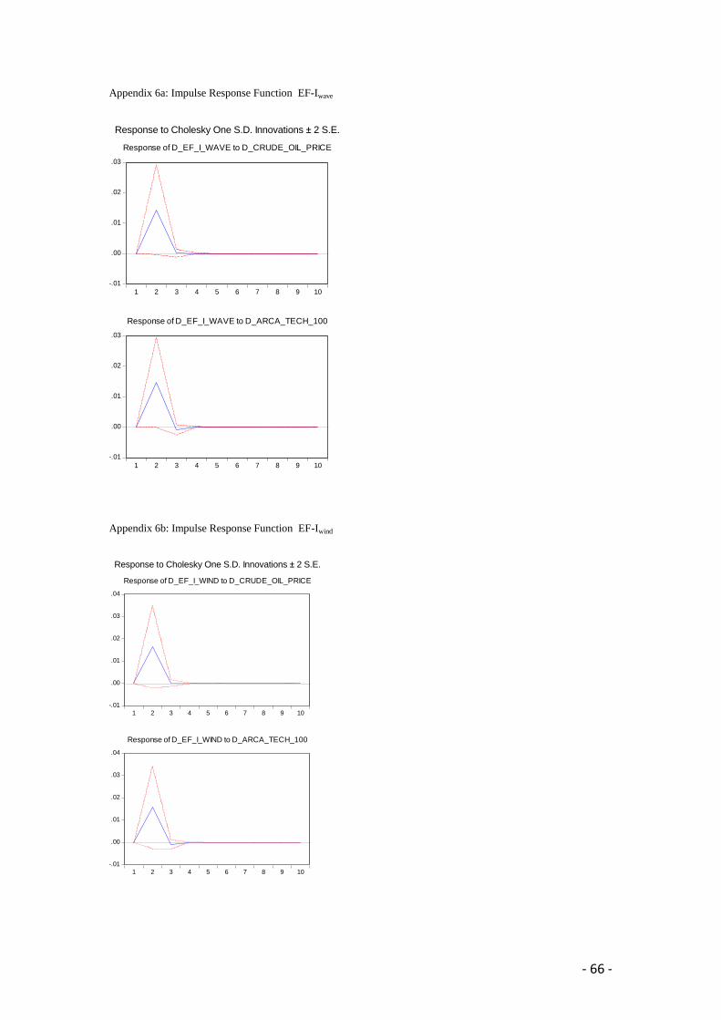
- 66 -

Appendix 6a: Impulse Response Function EF-Iwave

-.01

.00

.01

.02

.03

1 2 3 4 5 6 7 8 9 10

Response of D_EF_I_WAVE to D_CRUDE_OIL_PRICE

-.01

.00

.01

.02

.03

1 2 3 4 5 6 7 8 9 10

Response of D_EF_I_WAVE to D_ARCA_TECH_100

Response to Cholesky One S.D. Innovations ± 2 S.E.

Appendix 6b: Impulse Response Function EF-Iwind

-.01

.00

.01

.02

.03

.04

1 2 3 4 5 6 7 8 9 10

Response of D_EF_I_WIND to D_CRUDE_OIL_PRICE

-.01

.00

.01

.02

.03

.04

1 2 3 4 5 6 7 8 9 10

Response of D_EF_I_WIND to D_ARCA_TECH_100

Response to Cholesky One S.D. Innovations ± 2 S.E.

- 67 -

Appendix 6c: Impulse Response Function EF-Iphoto

Appendix 6d: Impulse Response Function EF-Ibio

-.02

.00

.02

.04

.06

.08

1 2 3 4 5 6 7 8 9 10

Response of D_EF_I_BIOSMASS to D_CRUDE_OIL_PRICE

-.02

.00

.02

.04

.06

.08

1 2 3 4 5 6 7 8 9 10

Response of D_EF_I_BIOSMASS to D_ARCA_TECH_100

Response to Cholesky One S.D. Innovations ± 2 S.E.

-.008

-.004

.000

.004

.008

.012

.016

.020

.024

1 2 3 4 5 6 7 8 9 10

Response of D_EF_I_PHOTOVOLTAICS to D_CRUDE_OIL_PRICE

-.008

-.004

.000

.004

.008

.012

.016

.020

.024

1 2 3 4 5 6 7 8 9 10

Response of D_EF_I_PHOTOVOLTAICS to D_ARCA_TECH_100

Response to Cholesky One S.D. Innovations ± 2 S.E.

- 68 -

Appendix 6e: Impulse Response Function EF-IR&D

-.02

-.01

.00

.01

.02

.03

.04

1 2 3 4 5 6 7 8 9 10

Response of D_EF_I_R_D to D_CRUDE_OIL_PRICE

-.02

-.01

.00

.01

.02

.03

.04

1 2 3 4 5 6 7 8 9 10

Response of D_EF_I_R_D to D_ARCA_TECH_100

Response to Cholesky One S.D. Innovations ± 2 S.E.

Appendix 6f: Impulse Response Function EF-Imanufacturing

-.02

-.01

.00

.01

.02

.03

.04

.05

1 2 3 4 5 6 7 8 9 10

Response of D_EF_I_MANUFACTURING to D_CRUDE_OIL_PRICE

-.02

-.01

.00

.01

.02

.03

.04

.05

1 2 3 4 5 6 7 8 9 10

Response of D_EF_I_MANUFACTURING to D_ARCA_TECH_100

Response to Cholesky One S.D. Innovations ± 2 S.E.

- 69 -

Appendix 6g: Impulse Response Function EF-Ireassembly

-.03

-.02

-.01

.00

.01

.02

.03

.04

1 2 3 4 5 6 7 8 9 10

Response of D_EF_I_RE_ASSEMBELY to D_CRUDE_OIL_PRICE

-.03

-.02

-.01

.00

.01

.02

.03

.04

1 2 3 4 5 6 7 8 9 10

Response of D_EF_I_RE_ASSEMBELY to D_ARCA_TECH_100

Response to Cholesky One S.D. Innovations ± 2 S.E.

Appendix 6h: Impulse Response Function EF-Iservices

.00

.04

.08

.12

1 2 3 4 5 6 7 8 9 10

Response of D_EF_I_SERVICES to D_CRUDE_OIL_PRICE

.00

.04

.08

.12

1 2 3 4 5 6 7 8 9 10

Response of D_EF_I_SERVICES to D_ARCA_TECH_100

Response to Cholesky One S.D. Innovations ± 2 S.E.

- 70 -

Appendix 6i: Impulse Response Function EF-Igeneration

-.02

-.01

.00

.01

.02

.03

.04

1 2 3 4 5 6 7 8 9 10

Response of D_EF_I_ENERGY_GENERATION to D_CRUDE_OIL_PRICE

-.02

-.01

.00

.01

.02

.03

.04

1 2 3 4 5 6 7 8 9 10

Response of D_EF_I_ENERGY_GENERATION to D_ARCA_TECH_100

Response to Cholesky One S.D. Innovations ± 2 S.E.