The impact of fiscal policy oneconomic activity over the business cycle –evidence from a threshold VAR analysis

Anja Baum(University of Cambridge)

Gerrit B. Koester(Deutsche Bundesbank)

Discussion PaperSeries 1: Economic StudiesNo 03/2011Discussion Papers represent the authors’ personal opinions and do not necessarily reflect the views of theDeutsche Bundesbank or its staff.

Editorial Board: Klaus Düllmann Frank Heid Heinz Herrmann Karl-Heinz Tödter

Deutsche Bundesbank, Wilhelm-Epstein-Straße 14, 60431 Frankfurt am Main, Postfach 10 06 02, 60006 Frankfurt am Main

Tel +49 69 9566-0 Telex within Germany 41227, telex from abroad 414431

Please address all orders in writing to: Deutsche Bundesbank, Press and Public Relations Division, at the above address or via fax +49 69 9566-3077

Internet http://www.bundesbank.de

Reproduction permitted only if source is stated.

ISBN 978-3–86558–690–2 (Printversion) ISBN 978-3–86558–691–9 (Internetversion)

Abstract:

Does the state of the business cycle matter for the effects of fiscal policy

shocks on GDP? This study analyses quarterly German data from 1976 to

2009 in a threshold SVAR, expanding the SVAR approach by Blanchard and

Perotti (2002). In a linear benchmark SVAR, the analysis finds that hiking

spending yields a short-term fiscal multiplier of around 0.70, while the fiscal

multiplier resulting from an increase in taxes and social security contributions

is -0.66. In addition, the threshold model derives fundamentally new insights

on the effects of shocks, depending on when in the business cycle they occur,

their size and their direction. Most importantly, fiscal spending multipliers

are much larger in times of a negative output gap but have only a very limited

effect in times of a positive output gap. Discretionary revenue policies, on

the other hand, have a generally more limited impact. Our findings have

important implications for the optimal fiscal policy mix over different stages of

the business cycle. Various robustness checks, including a different threshold

specification, do not influence these implications substantially.

Keywords: fiscal policy, business cycle, nonlinear analysis, fiscal multipliers

JEL-Classification: E62, E32, C54.

Non-technical summary

What are the effects of fiscal policy on economic growth? How effective

is it in smoothing the business cycle? Does the state of the business cycle

matter for the effects of fiscal policy shocks on GDP? These policy-relevant

macroeconomic questions are highly controversial, and the optimal fiscal policy

action with respect to the size, timing and the policy mix is the topic of fierce

debate in the literature.

This paper seeks to contribute to the empirical literature on fiscal policy

in Germany by adding an additional dimension to the usual linear analysis:

allowing for asymmetries of fiscal policy shocks on growth depending on their

size, their direction and their timing with respect to the business cycle. We

apply a threshold VAR approach, which is characterised by a separation of the

observations into different regimes based on a threshold variable, to model time

series non-linearities. Within each regime, the time series is then assumed to be

described by a linear model. In the baseline specification, we use the output

gap as the threshold variable as it divides economic development in phases

of under- and overutilisation – the two regimes under which we expect the

effects of fiscal stimuli to differ. To identify discretionary fiscal policy shocks,

we employ exogenously determined elasticities for the working of automatic

stabilisers.

Our research shows that short-term fiscal multipliers in Germany are in

general moderate and that the state of the business cycle strongly matters for

the effects of fiscal policy shocks. In a linear benchmark model, the analy-

sis finds that the effect of reductions in tax and social security contributions

and of increased spending on GDP each corresponds to a short-term fiscal

multiplier of around 0.7, putting it in the range of other empirical results for

Germany. In addition the threshold model derives fundamentally new insights

on the effects of shocks, depending on their timing with respect to the business

cycle. Most importantly, fiscal spending multipliers are much larger in times of

a negative output gap but have only a very limited effect in times of a positive

output gap. Discretionary revenue policies, on the other hand, have generally

a more limited effect. With respect to the cycle, their impact is larger in the

upper than in the lower output gap regime. Various robustness checks, in-

cluding a different threshold specification, do not influence the resulting policy

implications substantially.

Nichttechnische Zusammenfassung

Wie beeinflusst die Fiskalpolitik das Wirtschaftswachstum? Wie effektiv

ist ihr Einsatz zur Glattung des Konjunkturzyklus? Unterscheiden sich die

Effekte von fiskalpolitischen Stimuli abhangig von der aktuellen Auslastung

einer Okonomie? Diese wirtschaftspolitisch relevanten Fragen werden kontro-

vers diskutiert und uber die optimale Ausgestaltung fiskalpolitischer Impulse

hinsichtlich ihres Umfangs, ihrer Terminierung und der verwendeten Instru-

mente wird in der Literatur heftig gestritten.

Ziel dieses Papieres ist es, den ublicherweise in der Literatur zu find-

enden linearen Analysen der deutschen Fiskalpolitik eine weitere Dimension

hinzuzufugen, welche asymmetrische Reaktionen auf fiskalpolitische Schocks

abhangig von ihrer Große, ihrer Richtung und und ihrer Terminierung im

Konjunkturzyklus erlaubt. Dazu schatzen wir ein vektorautoregressives

”Schwellenwert-Modell”, welches die Analyse nicht-linearer Effekte durch

eine Einteilung der empirischen Beobachtungen in zwei unterschiedliche, in

Abhangigkeit von einem Schwellenwert definierte Regime ermoglicht. Inner-

halb jedes dieser zwei Regime wird dann ein lineares Modell angenommen. Im

Basismodell verwenden wir die Produktionslucke als Schwellenwert, da diese

den Konjunkturzyklus in Phasen der Unter- und der Uberauslastung aufteilt

- jene beiden Regime, in denen wir unterschiedliche Effekte von Fiskalstimuli

erwarten. Um die diskretionaren fiskalischen Schocks zu identifizieren verwen-

den wir exogen bestimmte Elastizitaten, die das Wirken der automatischen

Stabilisatoren abbilden. Unsere Analyse zeigt, dass die kurzfristigen Fiskal-

multiplikatoren in Deutschland generell begrenzt sind und dass die jeweilige

Position im Konjunkturzyklus einen wichtigen Einfluss auf die Wirksamkeit

von Fiskalstimuli hat.

In einem linearen Referenzmodell ergibt sich fur Kurzungen von Steuern

und Sozialabgaben und fur Ausgabenerhohungen zunachst ein kurzfristiger

Multiplikator von rund 0,7 - was im Bereich der Ergebnisse ahnlicher Studien

fur Deutschland liegt. Unser Schwellenwert-Modell ermoglicht daruber hinaus

grundlegend neue Einsichten in die Effekte von Schocks in Abhangigkeit von

ihrer Terminierung im Konjunkturzyklus. Wichtigstes Ergebnis ist dass die

Ausgabenmutliplikatoren in Zeiten der Unterauslastung deutlich großer sind

als in Zeiten der Uberauslastung. Diskretionare Einnahmenschocks dagegen

haben einen insgesamt geringeren Effekt als Ausgabenschocks. Hinsichtlich

der Terminierung im Konjunkturzyklus ist der Effekt von Einnahmenschocks

im oberen Regime großer als im unteren Regime. Diese Ergebnisse erweisen

sich als robust gegenuber zahlreichen getesteten Modifikationen des Modells -

einschließlich einer anderen Spezifizierung des Schwellenwertes.

Contents

1 Introduction 1

2 Empirical Literature 4

3 Methodology 8

4 The Data 12

5 Estimation 16

5.1 Model Specification . . . . . . . . . . . . . . . . . . . . . . . . . 16

5.2 Threshold Tests . . . . . . . . . . . . . . . . . . . . . . . . . . . 17

5.3 Identification . . . . . . . . . . . . . . . . . . . . . . . . . . . . 17

5.4 Impulse Response Analysis . . . . . . . . . . . . . . . . . . . . . 21

5.4.1 Linear Impulse Response . . . . . . . . . . . . . . . . . . 21

5.4.2 Lower Regime, 2% Growth Shock . . . . . . . . . . . . . 22

5.4.3 Upper Regime, 2% Growth Shock . . . . . . . . . . . . . 23

5.4.4 Comparison Lower and Upper Regime, Increasing Shock

Size . . . . . . . . . . . . . . . . . . . . . . . . . . . . . 24

6 Robustness Checks 25

6.1 GDP Growth Threshold . . . . . . . . . . . . . . . . . . . . . . 25

6.2 Structural Identification . . . . . . . . . . . . . . . . . . . . . . 26

6.3 Data Sample and Threshold Value . . . . . . . . . . . . . . . . . 27

7 Conclusions 28

A GIRF Algorithm 30

B Exogenous Elasticities 31

C Literature 33

List of Tables

1 German VAR Analysis, Impact of Fiscal Shocks on GDP . . . . 7

2 Unit Root Tests . . . . . . . . . . . . . . . . . . . . . . . . . . . 14

3 Descriptive Statistics . . . . . . . . . . . . . . . . . . . . . . . . 16

4 Tsay Threshold Test . . . . . . . . . . . . . . . . . . . . . . . . 17

5 Fiscal Multipliers . . . . . . . . . . . . . . . . . . . . . . . . . . 25

6 Calculated Elasticities . . . . . . . . . . . . . . . . . . . . . . . 31

7 Elasticities in the literature . . . . . . . . . . . . . . . . . . . . 32

List of Figures

1 Growth Rates of Series . . . . . . . . . . . . . . . . . . . . . . . 15

2 Output Gap Regimes, Threshold Value=0.15% . . . . . . . . . . 18

3 Time-Varying Elasticities . . . . . . . . . . . . . . . . . . . . . . 19

4 Adjusted Revenue - Output Gap Correlation . . . . . . . . . . . 19

5 Linear Impulse Responses, Shocks in R and G . . . . . . . . . . 22

6 Lower Regime: 2% Growth Shock . . . . . . . . . . . . . . . . . 23

7 Upper Regime: 2% Growth Shock . . . . . . . . . . . . . . . . . 24

8 Lower Regime: a1 = 0.5, 2% Growth Shock . . . . . . . . . . . . 39

9 Lower Regime: a1 = 1.5, 2% Growth Shock . . . . . . . . . . . . 39

10 Lower Regime: 1976-2008 . . . . . . . . . . . . . . . . . . . . . 40

11 Upper Regime: 1976-2008 . . . . . . . . . . . . . . . . . . . . . 40

12 5% Growth Shock - Lower Regime . . . . . . . . . . . . . . . . . 41

13 5% Growth Shock - Upper Regime . . . . . . . . . . . . . . . . 41

14 IR for GDP Growth as Threshold: 2% Growth Shock - Lower

Regime . . . . . . . . . . . . . . . . . . . . . . . . . . . . . . . . 42

15 IR for GDP Growth as Threshold: 2% Growth Shock - Upper

Regime . . . . . . . . . . . . . . . . . . . . . . . . . . . . . . . . 42

16 Lower Regime: Threshold of Zero - 2% Growth Shock . . . . . . 43

17 Upper Regime: Threshold of Zero - 2% Growth Shock . . . . . . 43

18 Lower Regime: Cholesky Order GDP → R → G . . . . . . . . . 44

19 Lower Regime: Cholesky Order R → G → GDP . . . . . . . . . 44

20 Upper Regime: Cholesky Order GDP → R → G . . . . . . . . . 45

21 Upper Regime: Cholesky Order R → G → GDP . . . . . . . . . 45

The Impact of Fiscal Policy on Economic

Activity over the Business Cycle -

Evidence from a Threshold VAR Analysis1

1 Introduction

What are the effects of fiscal policy on economic growth? How effective

is it in smoothing the business cycle? Does the state of the business cycle

matter for the effects of fiscal policy shocks on GDP? These policy-relevant

macroeconomic questions are highly controversial, and the optimal fiscal policy

action with respect to the size, timing and the policy mix is the topic of fierce

debate in the literature.

The financial turmoil in 2008/2009 has further strengthened the interest

of governments, central banks and academia in the role of fiscal policy. The

traditional monetary transmission mechanism is weak and monetary policy

alone seems unable to counter the huge contraction of demand. Furthermore,

many countries have nearly reached the zero lower bound, with no more room

to reduce central bank interest rates further. As a consequence, huge fiscal

stimulus packages have been introduced – in Germany as well as in most in-

dustrialised countries worldwide. And although the belief is strong that these

packages helped many countries to recover from the crisis, our knowledge of

the effectiveness of fiscal stimuli in such downturns – based on the theoretical

and empirical literature – is still very limited. This paper seeks to contribute

to the empirical literature on fiscal policy in Germany by adding an additional

dimension to the usual linear analyses, allowing for asymmetries of fiscal policy

shocks on growth depending on their size, their direction and their timing with

respect to the business cycle.

In the theoretical literature we find strongly diverging positions with re-

spect to the general effectiveness of fiscal stimuli. For example, standard Real

Business Cycle (RBC) models expect an increase in government consumption

to be completely offset by a reduction of private consumption (see Baxter and

1Authors: Anja Baum, University of Cambridge, email: ab862@hermes.cam.ac.uk; Ger-

rit B. Koester, Deutsche Bundesbank, email: gerrit.koester@bundesbank.de. The views

expressed in this paper are those of the authors and do not necessarily reflect the opinions

of the Deutsche Bundesbank or its staff. We thank Carsten Trenkler, Patra Geraats, Malte

Knuppel, Jorg Breitung, Karsten Wendorff, Christoph Priesmeier and Heinz Herrmann for

helpful comments and suggestions. The usual disclaimer applies.

1

King 1993, Christiano and Eichenbaum 1992 or Fatas and Mihov 2001). On

the other hand, standard Keynesian models argue that consumers are non-

Ricardian2 and a government consumption shock increases private consump-

tion and GDP (Blanchard 2001). However, so far little research effort has

been spent on the question of whether the effectiveness of fiscal policy might

vary depending on macro-economic circumstances. These effects can best be

covered in a non-linear policy analysis.3

There are several reasons why the reaction to fiscal stimuli can be non-

linear. Looking at the supply side of the economy, we can distinguish periods of

positive and negative output gaps. The traditional crowding out argument (see

Buiter 1977), stating that government expenditure replaces private spending,

is generally applicable in times of a positive output gap but less so in times

when output is below potential and excessive capacities in the economy are

available. This gives fiscal policy the chance to activate unused factors of

production.4

We also find several arguments for a non-linear impact analysis on the

demand side. For example, Drazen (1990) argues that the effects of fiscal

policy depend on the size and persistence of the fiscal impulse, because both

influence the signalling effect with respect to the fiscal policy that is to be

expected in the future (see Giavazzi et al. (2000) for empirical support).5

Additionally, in times of high negative output gaps and high unemployment

individuals and firms are facing tighter credit constraints, as banks eliminate

credit lines or increase the risk premia on interest rates for loans. Severely

credit-constrained borrowers tend to adjust spending substantially in response

to even a contemporaneous change in disposable income, which can even result

2The importance of non-Ricardian households for fiscal policy effects is discussed in

Coenen and Straub (2005), among others.3Corsetti et al. (2010) argue in favour of non-linear effects of fiscal policy, with especially

high fiscal multipliers after strong recessions. Christiano et al. (2009) state that fiscal policy

is most effective in the case of very low interest rates (which are likely to occur in times of

high negative output gaps).4Along these lines, Knuppel (2008) analyses the consequences of an inclusion of capacity

constraints in the RBC framework by means of a Markov switching model. He argues that

those capacity constraints are not binding in recessions, leaving economic agents more room

to react to policy measures.5The strong effects of the German government’s – massive fiscal stimulus packages –

including the “cash for clunkers” (“Abwrackpramie”) program – as well as financial market

stabilisation and the guarantee of deposits during the 2008/09 economic downswing can be

see as examples for such a signalling.

2

from a change in interest rates (see for example Jaaskela 2007). Although

the analysis of credit constraints has been applied mostly to monetary policy

research (see for example Blinder 1987, Galbraith 1996, Weise 1999, Balke

2000 and Calza and Sousa 2006), there is little reason to doubt that fiscal

policy can influence disposable income and thus consumption – especially that

of credit-constrained households – by tax cuts or by increases in transfers to

the most severely credit-constrained consumers and firms (for a discussion see

Galı et al. 2007 or Roeger and in’t Veld 2009).

If any of the arguments for non-linearity applies, the linear VAR framework,

which dominates the empirical literature, is not adequate. Tying a non-linear

economy to a linear VAR framework can lead to misleading inferences with

respect to its dynamics. Several approaches to model time series non-linearities

can be found in the literature, including Markov switching, smooth transition

and threshold autoregressive models. We adopt the latter approach, which is

characterised by a separation of the observations into different regimes based

on a threshold variable. Within each regime, the time series is then assumed

to be described by a linear model. In our multivariate context we use the

multivariate Tsay (1998) procedure to test for non-linearity in the data, using

the output gap or GDP growth as the threshold variable. In both cases the

test rejects linearity. Consequently, the threshold impulse responses (IR) are

generated using the general IR modelling introduced by Koop et al. (1996),

which allows for the non-linear propagation of shocks across regimes. Using

this framework, we can examine the sensitivity of economic activity to fiscal

policy shocks depending on the business cycle as well as of the size and the

direction of the shock.6

In the baseline specification, we use the output gap as the threshold vari-

able7, as it divides economic development in phases of under- and overutilisa-

tion – the two regimes under which we expect the effects of fiscal stimuli to

6Tong first proposed a threshold autoregressive (TAR) model in the late 1970s and refined

it during the early 1980s (Tong 1978, Tong and Lim 1980 and Tong 1983). Tsay (1998) and

Hansen (1996, 1997) made the threshold model applicable to a multivariate framework which

is now widely used in time-series analysis, as in Hansen (1999a, 1999b, 2000), Gonzalez and

Gonzalo (1997), Gonzalo and Montesinos (2000), Gonzalo and Pitarakis (2002), among

various others.7Koske and Pain (2008) demonstrate that the output gap plays an important role not

only for ex-post evaluation of policies but as well for real-time policy decisions. Furthermore

they argue that the output gap is a reliable real-time indicator in the short run.

3

differ.8

To identify discretionary fiscal policy shocks in our non-linear model, we

employ structural identification following Blanchard and Perotti (2002) and

hence use exogenously determined elasticities for the working of automatic

stabilisers. However, we extend their approach and estimate the impulse re-

sponses based on time-varying elasticities. This allows us to identify discre-

tionary fiscal policy shocks even more reliably.

Our research shows that short-term fiscal multipliers in Germany are in

general moderate and that the state of the business cycle strongly matters for

the effects of fiscal policy shocks. In a linear benchmark model, the analysis

finds that the effect on GDP of reductions in tax and social security con-

tributions and of increased spending each corresponds to a short-term fiscal

multiplier of around 0.7, putting it in the range of other empirical results for

Germany. In addition the threshold model derives fundamentally new insights

on the effects of shocks, depending on their timing with respect to the business

cycle. Most importantly, fiscal spending multipliers are much larger in times of

a negative output gap but have only a very limited effect in times of a positive

output gap. Discretionary revenue policies, on the other hand, have generally

a more limited effect. With respect to the cycle, their impact is larger in the

upper than in the lower output gap regime. Various robustness checks, in-

cluding a different threshold specification, do not influence the resulting policy

implications substantially.

The paper is organised as follows. Section 2 presents the main recent

empirical contributions in the literature, specifically for Germany. Section 3

subsequently presents the empirical approach, and section 4 includes a detailed

description of the dataset. The empirical strategy for structural identification

and the estimation results are presented in section 5. Various robustness checks

are carried out in section 6, and section 7 concludes.

2 Empirical Literature

The literature on fiscal policy multipliers derives strongly diverging results

for the effects of fiscal stimuli on economic activity. The methods applied

in empirical analyses range from model simulations using different estimation

8Within the robustness checks we pursue an analysis that employs a three-quarter moving

average of GDP growth itself as threshold.

4

and calibration techniques – such as the IMF Multimod model, the OECD

Interlink or the ESCB New Area Wide Model - to reduced form equation

parameter estimation techniques. Surveys of the empirical literature, which

can be found in Hemming (2002), Spilimbergo et al. (2009) and Coenen et al.

(2010), demonstrate the great bandwith of spending and revenue multipliers.

Depending on the method and model specification, one-year fiscal spending

multipliers range between 0.2 and 2 for the US, while estimates for Germany

lie between -0.2 and 5.1.9

While no consensus on the impact of fiscal policy on economic activity has

been reached, researchers generally agree on the importance of interdependen-

cies between fiscal and economic developments. Within the empirical literature

these interdependencies are most frequently analysed in vector autoregressive

(VAR) models. A focus in this literature lies on the identification of discre-

tionary fiscal policy shocks, for which most researchers rely on some form of

structural identification.10 Most prominent are the recursive identification ap-

proach (Cholesky ordering), the sign-restrictions approach11 and the structural

VAR approach using the identification procedure proposed by Blanchard and

Perotti (2002) (for a discussion on Cholesky ordering and sign-restrictions see

Perotti 2004).

In the present paper we follow Blanchard and Perotti (hereafter BP). BP

identify automatic stabilisers by incorporating exogenously given information

about the elasticities of revenues and expenditures with respect to GDP. In

their 2002 paper, they analyse the US economy between 1960 and 1997 and

find that expansionary fiscal shocks increase output with a long-term fiscal

multiplier close to unity. Furthermore, they find negative effects of tax and

spending increases on investment.

It is important to note that the results obtained from VAR studies depend

on the specific country analysed, as fiscal policy, the structure of the econ-

omy and the interplay of economic and fiscal developments differ substantially

9However, the value of 5.1 is derived by Perotti (2006) only for public investment spend-

ing.10The narrative or event-study approach can also be used for identification. It identifies

discretionary policy actions via specific historical events, such as contemporaneous press

reports, wars or war-related military spending, tax changes and elections. For further dis-

cussion see Ramey and Shapiro (1998), Edelberg et al. (1999), Eichenbaum and Fisher

(2005), Ramey (2006) and Favero and Giavazzi (2009) or Romer and Romer (2010).11For a current application to US data see Mountfort and Uhlig (2009), who find the

highest multipliers for deficit-financed tax cuts.

5

across countries. Therefore, the analysis of shocks based on German data is

likely to yield different results than those for the US.12 For Germany only a few

attempts analysing fiscal policy shocks are available, and all but one of them

employ the BP identification approach. The studies include Hoppner (2001),

Perotti (2004), Heppke-Falk et al. (2010) and Bode et al. (2006). Afonso and

Sousa (2009) employ a recursive identification.13

Hoppner (2001) uses quarterly cash data from 1970 to 2000 in a three-

variable VAR (government expenditures including government consumption,

investment and public transfers, such as subsidies; tax revenues from direct

and indirect taxes; and GDP). Based on his estimations, the effects of tax

shocks are by far larger than the effects of spending shocks. He estimates a

significant fiscal multiplier for a tax increase of -1.59 in the long run (meaning

that a tax increase by one unit reduces GDP by more than 1.5 units), while

the multiplier for an expenditure shock equals only 0.23 (and is insignificant).

Perotti (2004) applies the BP approach to various countries, including Ger-

many, and analyses the effects of fiscal shocks on output, inflation and the ten

year nominal interest rate. In his data set public spending is restricted to

public investment and consumption and does not include interest spending,

while the net revenue series is calculated by subtracting transfers from overall

revenues. Perotti argues that tax-financed transfers have the reverse effects of

taxes and should therefore be substracted from overall taxes. For Germany

Perotti uses quarterly West German data from 1960 to 1989. Based on these

data definitions, he finds a short-term multiplier of only around 0.5 following a

positive shock of government spending, which fades out quickly after the first

year.

Furthermore, Perotti identifies a structural break in 1974 and re-estimates

the model in two subperiods (1960-1974 and 1975-1989). The structural break

influences especially the effect of tax shocks. In the first subsample he estimates

a short-term multiplier of 0.19 (after 4 quarters) for tax increases – indicating

an expansionary effect of tax hikes - while in the second subsample the tax

multiplier for a positive shock is -0.03.

Heppke-Falk et al. (2010) follow the Perotti (2004) data definitions and

12This is demonstrated by Burriel et al.(2010), who compare the effects of fiscal policy

in the US and the Euro area using the BP approach and find a much higher persistency of

fiscal shocks in the US.13A detailed comparison of the first three VAR studies for Germany can be found in Roos

(2007).

6

Table 1: German VAR Analysis, Impact of Fiscal Shocks on GDP

Sample short-run long-run

Effect of an increase in government spending on GDP

Hoppner (2001) 1970-2000 positive insignificant

Perotti (2004)a 1960-1989 positive insignificant/negative

Heppke-Falk et al. (2010) 1974-2008 positive* positive*

Bode et al. (2006) 1991-2005 positive insignificant

Afonso and Sousa (2009) 1980-2006 negative negative

Effect of a decrease in government revenues on GDP

Hoppner (2001) 1970-2000 positive positive

Perotti (2004)a 1960-1989 negative/insignificant insignificant

Heppke-Falk et al. (2010) 1974-2008 positive** insignificant

Bode et al. (2006) 1991-2005 positive insignificant

Afonso and Sousa (2009) 1980-2006 insignificant negative

* Significant only for government investment; in sum with government consumption insignificant

** Significant only for direct taxes; net revenue is insignificant

a : Two subsamples are tested, the first 1960-1974, the second 1975-1989. If the results are different,

they are shown for the first and the second subsample, respectively.

estimate a VAR covering a longer time series of quarterly German cash data

between 1974 and 2008. In their three variable specifications (GDP, expendi-

ture and revenues), they find a positive reaction of GDP to spending increases

that is significant only in the contemporaneous quarter, with a spending multi-

plier of around one. Like Perotti’s first subsample, they find a positive reaction

of GDP to a revenue increase with a value of 0.12 in the quarter the shock

occurs.

Bode et al. (2006) estimate the structural three-variable VAR including

only pan-German data from 1991-2005. Based on a data definition similar to

that of Perotti (2004) and Heppke-Falk et al. (2010) they find a significant

positive effect of spending on GDP, with a one-year fiscal multiplier of around

0.5, as well as a significantly negative but in size slightly smaller multiplier for

the effects of a revenue increase.

The latest available study for Germany is provided by Afonso and Sousa

(2009), who use a Cholesky decomposition for the structural identification in

a nine-variable VAR covering data from 1980 to 2006. They further add a

feedback rule in order to cover government debt dynamics, and find a small

but significant fall in GDP after a spending shock. The reaction of GDP to a

revenue increase is small but positive, supporting the finding by Perotti (2004)

for the first subsample. They explain these results with a “crowding-out”

effect of public spending, but also a “crowding-in” effect of public revenues,

with both consumption and investment increasing after the shock as a result

of fiscal consolidation.

In summary, all the studies which use the BP identification scheme find a

small positive fiscal multiplier for government spending increases, while Afonso

7

and Sousa (2009) estimate a small but negative effect based on a Cholesky

identification. With respect to tax cuts, the results of the discussed studies

differ strongly. Tax cuts increase GDP in the studies by Hoppner (2001) and

Bode et al.(2006), while Heppke-Falk et al. (2010) and Afonso and Sousa

(2009) find contractionary effects. Perotti’s (2004) results are sensitive to

the subsample analysed. Depending on the timespan covered, the impulse

responses display clear differences and therefore indicate a variability of the

impact of fiscal shocks in different decades and macroeconomic environments.

Closely related to this last point, a drawback of all the empirical studies

presented is that they are bound to a linear estimation framework. That

is, they do not account for any asymmetry in the variable responses or the

relationship between the macro variables themselves. However, since they

provide a good starting point for a fiscal policy analysis, we use the linear

modelling as a benchmark and extend it to a non-linear threshold framework in

order to account for the possible asymmetries discussed in the introduction.14

3 Methodology

Threshold VARs are piecewise linear models with different autoregressive

matrices in each regime. The regimes are determined by a transition vari-

able, which is either one of the endogenous variables or an exogenous variable

(Hansen 1996, 1997, Tsay 1998). In general it is possible to obtain more than

one critical threshold value and therefore more than two regimes, but for sim-

plicity we will focus on a model with two regimes only.15

Let a set of k stationary endogenous variables with yt = (y1t, ..., ykt)′ and

T observations describe a VAR of finite order p

yt = Γ0 + Γ1yt−1 + ... + Γpyt−p + ut , (1)

where Γ0 is a k-dimensional vector containing deterministic terms such

as a constant, a linear time trend or dummy variables. Γi with i = 1, ..., p

are squared coefficient matrices of order k, and ut is a sequence of serially

uncorrelated random vectors with mean zero and covariance matrix Cov(ut) =

Σu. We can rewrite equation (1) in the compact form

yt = ΓXt + ut , (2)

14An interesting non-linear analysis of German fiscal policy using a different methodology

is Hoppner and Wesche (2000), who apply a Markov-switching approach to fiscal policy

effects in Germany and find time-varying effects.15The two-regime setup is also best for our fiscal policy analysis over the business cycle

since the general concept of the business cycle is based on a distinction between an upper

(positive output gap) and a lower (negative output gap) regime.

8

with Γ = (Γ0, Γ1, ..., Γp) and Xt = (1, yt−1, ..., yt−p)′. Following this nota-

tion, a threshold VAR is represented by

yt = Γ1Xt + Γ2XtI[zt−d ≥ z∗] + ut . (3)

zt−d is the threshold variable determining the prevailing regime of the sys-

tem, with a possible lag d. I[·] is an indicator function that equals 1 if the

threshold variable zt−d is above the threshold value z∗ and 0 otherwise. The

coefficient matrices Γ1 and Γ2, as well as the contemporaneous error matrix

ut are allowed to vary across regimes. The delay lag d and critical threshold

value z∗ are unknown parameters and determined alongside the parameters.

In the linear and the non-linear model we face the problem that the con-

temporaneous errors are not uncorrelated with each other, i.e. Σu is not a

diagonal matrix. In this case fiscal policy shocks are not identified, since the

correlation of the error terms indicate that a shock in one variable is likely

to be accompanied by a shock in another variable. Following Blanchard and

Perotti (2002), we identify the policy shocks using an AB model for structural

identification in the error-covariance matrix. The linear model thus becomes16

Ayt = CXt + Bεt , (4)

assuming that ut = A−1Bεt where Σu = A−1BB′A−1′ and B is a k × k

matrix of parameters.17

The non-linear model can be correspondingly written as

Anyt = C1Xt + C2XtI[zt−d ≥ z∗] + Bnεnt , (6)

where An and Bn differ from A and B in the linear model, since they are

based on the regime-dependent errors. As before, Γi = A−1i Ci, and Cov(un

t ) =

Σn = A−1n BnB′

nA−1n . The exact identification procedure is explained in section

5.3.

Before estimating a non-linear model we need to test if the system is indeed

non-linear. Following the testing approach developed by Tsay (1989, 1998) we

first identify a series z representing the threshold variable with −∞ = z0 <

z1 < ... < zs−1 < ∞. z needs to be stationary with a continuous distribution,

restricted to a bounded set S = [z, z], where S is an interval on the full sample

16A detailed description and derivation of the AB model, as well as the corresponding

A and B models can be found in Amisano and Giannini (1997), Lutkepohl (2005) and

Lutkepohl and Kratzig (2004). Further applications of the AB model can be found in Pagan

(1995), Breitung and Lutkepohl (2004) and Blanchard and Perotti (2002).17Alternatively, the AB model can be represented in the error component form

Aut = Bεt . (5)

9

range of the threshold variable. The interval should be trimmed in order to

assure a minimum number of observations in each subsample.

The lag order p and the threshold lag d need to be determined a priori,

which in case of p is achieved by applying the normal information criteria in the

linear VAR estimation. For the choice of d we will rely on economic reasoning.

The regression framework of equation (2) can be rewritten as

y′

t = X ′

tΓ + u′

t, t = h + 1, ...n , (7)

where, as before, Γ denotes the parameter matrix, Xt = (1, y′

t−1, ..., y′

t−p)′,

and h = max(p, d).

We reorder the cases according to the threshold variable zt−d, denoting the

i-th smallest element of the interval S as z(i) (equals the m-th smallest value

of all observations.18) The arranged regression can be written in the form

y′

t(i)+d = X ′

t(i)+dΓ + u′

t(i)+d, i = 1, ..., n − h (8)

where t(i) is the time index of z(i). In short, we order the values of the

threshold variable according to its size and split the sample according to the

threshold value z(i). The model is estimated with the m observations below

z(i) by OLS to obtain Γ′

m. Subsequently, OLS is performed again for the

first m + 1 observations with z(i + 1) and so on. The result is a sequence of

OLS regressions, each using the first m ranked observations. For each of these

regressions, we keep the one-step ahead predictive and standardised residuals

� and η, calculated with

�t(m+1)+d = yt(m+1)+d − Γ′

mXt(m+1)+d (9)

ηt(m+1)+d =�t(m+1)+d

[1 + X ′

t(m+1)+d(Σmi=1Xt(i)+dX

′

t(i)+d)−1Xt(m+1)+d]1/2

. (10)

In order to analyse threshold behaviour we test for white noise in the re-

gression

η′

t(l)+d = X ′

t(l)+dφ + w′

t(l)+d, l = m0 + 1, ..., n− h (11)

where m0 denotes the starting point of the recursive least squares estima-

tion. If φ = 0 the data is generated by a linear model.19 Consequently, we

18Remember that the interval S = [z¯, z] is trimmed. The trimming percentage is the

percentage of observations of the whole sample below m0. m0 corresponds to z(i) with

i = 1.19The sequential OLS estimates are consistent estimates of the lower regime parameters

as long as the last observation used in the regression does not belong to the upper regime.

In this case, the predictive residuals are orthogonal to the corresponding regressor and yt is

linear. However, if yt follows a threshold model, the predictive residuals will not be white

noise and correlated with Xt(i+d). As a consequence the least squares estimator would be

biased.

10

test the hypothesis H0 : φ = 0 against the alternative H1 : φ �= 0. Tsay (1998)

proposes the following test statistic:

C = [n − h − m0 − (kp + 1)]{ln[det(S0)] − ln[det(S1)]} (12)

with det(·) being the determinants of

S0 =1

n − h − m0

n−h∑l=m0+1

ηt(l)+dη′

t(l)+d (13)

and

S1 =1

n − h − m0

n−h∑l=m0+1

wt(l)+dw′

t(l)+d. (14)

The test statistic is asymptotically chi-square with k(pk + 1) degrees of

freedom. If the test detects a threshold in the DGP, the coefficients can be

estimated conditional on a sum of least square minimisation over both regimes.

That is, for a given value of z, the LS estimate of Γ(i) for regimes (i) = 1, 2 is

Γ(i)(z) = (

(i)∑t

Xt(z)Xt(z)′)−1(

(i)∑t

Xt(z))yt (15)

with residuals ut(i)(z) = yt − Xt(z)′Γ(i)(z), and residual variance

σ2(i)(z) =

∑(i)t u 2

t(i)(z)

n(i) − k, (16)

where∑(i)

t is the sum of all observations in regime (i) and n(i) is the number

of observations in regime (i). The sum of squared residuals is

R(z) = R(1)(z) + R(2)(z) , (17)

where R(i)(z) = (n(i) − k)σ2(i)(z). Finally, the conditional threshold value

z∗ is obtained by

z∗ = argminzR(z) . (18)

In the case of a test result that suggests a threshold effect, we wish to

apply an impulse response (IR) analysis that is able to capture non-linearities.

Gallant et al. (1993), Koop (1996) and Koop et al. (1996) point out that

in non-linear models the effect of a shock depends on the entire history of

the system up to the point when the shock occurs. Thus, it is necessary to

model the IRF conditional on this history, and as a consequence conditional

11

on the size and the direction (sign) of the shock.20 For this purpose we cannot

apply linear IR functions, as they are history-independent, i.e. they do not

depend on a particular history of the data up to time t. They are symmetric

in the sense that a shock of −εt−m has exactly the opposite effect of a shock

of size +εt−m and they are linear as they are proportional to the size of the

shock. Hence, they cannot be applied here. Instead, we will model generalised

impulse response functions (GIRF) introduced by Koop et al. (1996), which

address these problems and which are applicable to both linear and non-linear

models.

Defining εt as a shock of a specific size, m as the forecasting horizon and

Ωt−1 as the history or information set at time t− 1, Koop et al. (1996) define

the GIRF as the difference between two conditional expectations with a single

exogenous shock:

GIRF = E[Xt+m|εt, εt+1 = 0, ..., εt+m = 0, Ωt−1]

− E[Xt+m|εt = 0, εt+1 = 0, ..., εt+m = 0, Ωt−1] . (19)

The GIRF allows the regimes to switch after a shock, a characteristic that

is responsible for the different outcomes of positive and negative shocks as well

as their size.21. We are thus able to relax the assumption that shocks occur-

ring in a recession are just as persistent as shocks occurring in an expansion.

The calculation of the GIRF induces some computational effort and the exact

algorithm is described in Appendix (A).

4 The Data

To keep the analysis as parsimonious as possible, we include only three vari-

ables: government spending, government revenue and GDP.22 In the non-linear

specification, we need an additional threshold variable in order to distinguish

between ”good” and ”bad” economic times. Here we rely on the output gap as

an indicator for the different phases of the economic cycle, which is generally

20In fact, non-linear time series models do not have a Wold representation and the as-

sumption that no shocks occur in intermediate periods may give rise to misleading inferences

concerning the propagation mechanism of the model.21GIRF were applied in several empirical applications, for example in Balke (2000),

Atanasova (2003), Root and Lien (2003), Jaaskela (2007) A detailed description of GIRF

for the univariate case can also be found in Potter (2000).22A five-variable model that contains investment and consumption might allow us to study

the transition of policy shocks in the economy in more detail, but estimating a five-variable

model is impractical because the number of coefficients in the linearity test and the TVAR

rises in proportion to the number of coefficients in the standard linear model. This affects the

size and power of the tests. Therefore, the present paper will restrict itself to a three-variable

specification and leaves the proposed extension to future work.

12

seen not only as a reliable ex-post but also as a reliable real-time indicator for

policy-makers (see Koske and Pain 2008).

The data is compiled from the Deutsche Bundesbank’s national accounts

database and defined according to the European System of National Accounts

(ESA) 1979 and 1995. The advantage the national accounts data has over cash

data is that its data are adjusted for special events and distortions caused, for

example, by lagged payments of taxes.23 Additionally, we remove the effect of

the liquidation of the German Treuhand in 1995 (199.6 billion Euro in total)

and revenues from the auction of the UMTS licenses in 2000 (50.8 billion Euro).

The dataset is quarterly and covers the period from the first quarter of

1976 to the fourth quarter of 2009, giving 136 observations. Generally we

would have been able to start our analysis in the first quarter of 1970, but

we decided to exclude the first five years in order to avoid a structural break

due to a policy shift after 1975.24 The structural break at reunification is

eliminated by prolonging the series for reunified Germany backwards with

West German growth rates. Our estimations are based on data in real terms

(all three variables are deflated by the GDP deflator with a value of 1 in the

year 2000) and seasonally adjusted by applying the BV 4.1 procedure of the

German Federal Statistical Office.25

The output gap is calculated with the Hodrick-Prescott filter (λ = 1600)

applied to the real GDP series. To avoid a distortion of the results at the lower

and upper bound, we prolong the series with its own linear trend in the past

(1960-1970) and the future (2009-2019). The real output gap variable is then

calculated as the difference between actual real GDP and potential real GDP

(measured by the HP-filtered trend) as a percentage of potential GDP.

The fiscal series offer a great variety of possible compositions. Seminal stud-

ies such as BP (2002) and Perotti (2004) define public spending very narrowly

as government investment plus government consumption, and public revenues

as general government revenues (excluding social security) minus transfers. Al-

though many papers follow this definition (see the discussion in section 2), we

argue that it is not well-suited for an analysis of fiscal policy in Germany, since

social insurance accounts on average for more than 40% of total revenues and

23See ECB (2007) for a definition of government finance statistics according to ESA and

standard methods of national accounting.24Before 1976 the German government - inspired by Keynesian macro-economics - aimed

at an active stabilisation of the business cycles via frequent temporary tax and expenditure

measures. The most important measure aimed at economic stimulation was the introduction

of an investment bonus of 7.5% for all investment in machinery and equipment realised

between 1 December 1974 and 30 June 1975. These measures contributed to a high volatility

of tax revenues and spending, which is reflected especially in the growth rates of the series,

with a breakpoint identified by Perotti (2004), for instance, to be 1974:4.25A discussion of the methodology applied in the ”Berliner Verfahren” can be found at

http://www.uni-mannheim.de/edz/pdf/eurostat/06/KS-DT-06-012-EN.pdf.

13

Table 2: Unit Root Tests

ADF Phillips-Perron

Lags (SIC) t-statistic p-value t-statistic p-value

Revenues 7 -4.274 0.0007 -8.984 0

Expenditures 3 -5.388 0 -11.721 0

GDP 1 -4.914 0.0001 -6.999 0

Output Gap 9 -5.155 0 -3.705 0.005

H0: series has a unit root.

for a large part of overall public spending. Furthermore, economic stimulation

is often explicitly pursued via the social security system. For example, during

the 2008/2009 recession large parts of the German fiscal stimulus were imple-

mented through deficit-financed cuts in social security contributions. Even if

considered as a pure redistribution (such as in Perotti 2004, Heppke-Falk et

al. 2010, or Bode et al. 2006), the social security system can have far-reaching

effects on private consumption based on differences in the savings rate of net

payers and net recipients. These consumption effects, in turn, can influence

overall growth. Thus, we include social insurance in our analysis.

Unemployment spending is, due to its strong dependence on the business

cycle, subtracted from the expenditure side and enters the revenue series with

a negative sign in order to satisfy the precondition of the BP structural identifi-

cation approach that automatic stabilisers only apply on the revenue side. The

treatment of public interest spending differs over the existing studies. Perotti

(2004) and Fernandez and Cos (2006) argue that interest spending is not part

of discretionary fiscal policy and should be excluded from the data series, while

Blanchard and Perotti (2002) argue that interest payments should be included

as they reflect a ”normal” transfer of resources from the public to the private

sector (and thereby influence economic growth). We follow the approach of

Perotti (2004) and subtract interest payments from the expenditure and the

revenue variable.26

Taken together, this leaves us with a public spending series defined as total

current public spending excluding net interest (i.e. interest spending minus

dividends received by the government) and unemployment insurance spending.

Our revenue series includes social security contributions but is diminished by

net interest spending and unemployment insurance spending.

Except for the output gap (which is stationary), we apply the logarithm

to all series and take the first differences in order to achieve stationarity. The

resulting quarter-to-quarter growth rate series and the output gap are plotted

in figure 1. All series tend to revert to their mean.

26This approach is in line with other studies for Germany, such as Heppke-Falk et al.

(2010) and Bode et al. (2006).

14

Figure 1: Growth Rates of Series

-.02

-.01

.00

.01

.02

.03

80 85 90 95 00 05

Expenditures

-.04

-.03

-.02

-.01

.00

.01

.02

.03

80 85 90 95 00 05

GDP

-.03

-.02

-.01

.00

.01

.02

.03

.04

80 85 90 95 00 05

Revenues

-.03

-.02

-.01

.00

.01

.02

.03

.04

80 85 90 95 00 05

Output Gap

15

Table 3: Descriptive Statistics

Variable Mean Maximum Minimum Std. Dev.

Revenues 0.0049 0.031 -0.026 0.012

Expenditures 0.0039 0.021 -0.013 0.007

GDP 0.0048 0.023 -0.033 0.007

Output Gap -0.0001 0.036 -0.029 0.014

We also employ the standard unit-root methodology, i.e. the Augmented

Dickey-Fuller (ADF) and Phillips-Perron test. It is necessary to choose the

number of augmentation lags to account for serial correlation in the Dickey-

Fuller regressions, for which we use the Schwarz Information Criterion (SIC).

For all four series, both tests include a constant but no trend. Table 2 shows the

results for the growth rates. The values indicate that the series are stationary

by rejecting the null hypothesis of the existence of a unit root. Additionally,

descriptive statistics of the three series are shown in table 3.

5 Estimation

5.1 Model Specification

The VAR of equation 1 consists of a three-dimensional system of endoge-

nous variables yt = [Tt, Gt, GDPt], with Tt, Gt and GDPt being the growth

rates in government revenues, government spending and GDP, respectively. A

constant is included in yt.

For the optimal lag length we conduct various model selection tests, which

provide different lag order suggestions. While the Schwarz Information Crite-

rion (SIC) suggests the use of only one lag, the Akaike Information Criterion

(AIC) and the Hannan-Quinn (HQ) Criterion suggest the use of four lags

and the prediction error the use of six. Although the majority of the criteria

propose a higher order, we follow the SIC and specify the benchmark speci-

fication with one lag. We base this choice on the same reason for using only

three variables: the high cost of estimating additional parameters and there-

fore of over-fitting in the non-linear model (every additional parameter added

decreases the power of the estimation substantially; see for example Hansen

(1996) for a Monte Carlo proof).

Using one lag in the VAR, the Breusch-Godfrey Lagrange multiplier test

for serial correlation does not reject the null hypothesis of no serial correlation

for the tested lag numbers 2 and 5 with p-values of 0.115 and 0.218, respec-

tively. On the other hand, the Portmanteau test does reject the null at least

at the 5% level for higher lag values.27 It is thus important to check the model

27However, the same is true if the model is estimated with four and six lags. Therefore

we do not base the choice of the lag order on the autocorrelation properties.

16

Table 4: Tsay Threshold Test

d Test statistic p-valuea Threshold value

0 19.971 0.0676 -0.001516

1 39.916 0.0000 -0.001510

2 32.138 0.0013 -0.001516

H0: linearity, H1: threshold behavior

d: lags in the threshold variable

estimation properties in a profound robustness analysis. Furthermore, since

the standard errors might be underestimated, we have to be careful in inter-

preting the confidence regions. To rule out that the policy implications we will

find rely to a great part on imprecise structural identification, we will test the

effects of alternative values for a1 as well as changes in the general identifica-

tion procedure through the application of the Cholesky decomposition in the

robustness checks.

5.2 Threshold Tests

The test results for the null of linearity with one lag in the VAR and

different lags in the output gap are presented in table 4. The Tsay test statistic

is computed using a 30% trimming percentage and the test rejects linearity

of the system for all three threshold specifications. We will continue to use

one lag in the threshold variable, in order to account for moderate economic

rigidities.

The estimated threshold value for a specification with one lag in the VAR

and one lag in the threshold variable is -0.0015. Being in close neighbourhood

to zero, this value justifies the classification of the two regimes as representing

periods of output above and below its potential level. The two regimes are

shown in figure 2. The sample splits into 45 observations in the lower regime

and 91 observations in the upper regime, with a total of 15 regime switches.

With two of those being of very short length, this gives us approximately six

complete business cycles within 39 years.

5.3 Identification

As described earlier, we follow the identification procedure developed by

Blanchard and Perotti (2002). In the SVAR representation Aut = Bεt, ut =

(gdpt, gt, tt) is the vector of reduced-form error terms for the GDP, government

spending and revenue equation, respectively. The vector of structural shocks

is given with εt = (εGDPt , εT

t , εGt ) with Cov(εt) = I3 and εGDP

t , εGt and εT

t

corresponding to the GDP, tax and spending shocks. After estimating the

reduced form VAR, we can use the reduced-form residuals ut to determine the

elements of A and B. But prior to that, some identifying assumptions need to

17

Figure 2: Output Gap Regimes, Threshold Value=0.15%

-.006

-.004

-.002

.000

.002

.004

.006

1980 1985 1990 1995 2000 2005

OUTGAP THRESH

be made. First, the innovation in the fiscal variables gt and tt can be described

as a linear combination of three types of shocks, (i) the automatic response

of government expenditure and revenue to real output, (ii) the systematic,

discretionary response of expenditure to shocks in revenue and of revenue to

shocks in expenditure and (iii) the random, discretionary fiscal policy shocks,

which are the underlying structural shocks εGt and εT

t to be identified. We

also think of unexpected changes in GDP (gdpt) as a function of shocks in

government spending, revenue and a structural shock in GDP itself. With

these assumptions, we can write:

tt = a1εGDPt + a2ε

Gt + εT

t

gt = b1εGDPt + b2ε

Tt + εG

t (20)

gdpt = c1εTt + c2ε

Gt + εGDP

t .

We can rearrange this system to reconstruct the AB representation Aut =

Bεt, with

A =

⎛⎝

1 0 −a1

0 1 −b1

−c1 −c2 1

⎞⎠ and B =

⎛⎝

1 a2 0

b2 1 0

0 0 1

⎞⎠ . (21)

Using information about the tax and transfer system to determine the

coefficients in A and B, Blanchard and Perotti apply the following procedure:

I) In the first step institutional information on the German public finance

system is used in order to identify the coefficients a1 and b1. We have to

consider that the two coefficients incorporate two distinct effects of activity

on spending and taxes. They capture the automatic stabilisers, which are the

automatic effects of economic activity on the fiscal variables under existing

18

0.95

0.96

0.97

0.98

0.99

1.00

1.01

1.02

1.03

1970 1975 1980 1985 1990 1995 2000 2005

Figure 3: Time-Varying Elas-

ticities

-.04

-.03

-.02

-.01

.00

.01

.02

.03

.04

.05

-.03 -.02 -.01 .00 .01 .02 .03 .04

Output Gap

Ad

juste

d R

eve

nu

es

Figure 4: Adjusted Revenue - Output

Gap Correlation

fiscal institutions. In addition, they capture any discretionary adjustment

of fiscal policy to unexpected exogenous changes in economic activity within

the same quarter. As long as we assume that it takes fiscal policy to react

some time to changes in GDP due to democratic, legislative and bureaucratic

processes in decision making and implementation, the use of quarterly data

basically eliminates the second channel. It is thus valid to assume that a1

and b1 solely capture the automatic responses of fiscal variables to GDP. They

are calculated using the OECD framework by Girouard and Andre (2005), the

difference being that we use quarterly instead of annual data. For the aggregate

elasticity of N tax series with respect to output Girouard and Andre (2005)

apply the following formula:

a1 =

N∑i=1

ηTi,BiηBiGDP

Ti

T(22)

where T are the net taxes, with T =∑N

i Ti and Ti being taxes of type

i, which take on a positive value for taxes and a negative value for transfers.

ηTi,Bidenotes the elasticity of tax i with respect to its tax base Bi and ηBiGDP

denotes the elasticity of the tax base to GDP. The exact calculation of the

elasticity a1 and the taxes and tax bases in use are described in Appendix (C).

Following the OECD approach, we find an elasticity around 1, which lies in

the middle of elasticities applied in studies relying on similar data.28

However, one could object that the shares of the different revenue and

expenditure components in net revenues vary strongly over time, which we

demonstrate in figure 3. Even if the elasticities of the subcomponents were

stable - this would make the application of time-varying elasticities necessary.

In this respect we extend the basic BP approach and use the time-varying

elasticities instead.

28We also estimate the model based on elasticities of 0.5 and 1.5 to test the robustness of

our results; see section 5.1.

19

Additionally, we test the viability of the applied elasticities through corre-

lation between the output gap and the revenue series, which we adjusted for

the automatic responses based on the calculated elasticity. A non-zero corre-

lation means that the elasticities are misspecified and discretionary shocks not

precisely identified. Figure 4 shows the regression result and the scatter-plot

of the output gap on the x-axis and the adjusted growth rates of revenues on

the y-axis. We detect no correlation between the two series, which speaks in

favour of the elasticity applied and indicates that non-linearity is more likely to

be rooted in discretionary fiscal policy reactions than in automatic stabilisers.

The identification of b1 is easier. It can be set to zero, as the main com-

ponent of primary government spending (unemployment transfers) is included

in net revenues.

II) In the second step, we construct the contemporaneous influence of rev-

enues and expenditure on GDP, c1 and c2. With the estimates of a1 and b1

the cyclically adjusted reduced-form fiscal policy shocks (revenue and spend-

ing residuals) are calculated with t′t = tt − a1gdpt and g′

t = gt − b1gdpt = gt.

These can be used as instrument variables in the third equation of system (16).

They are considered as instruments since they are no longer correlated with

εGDPt (though still correlated with each other). Therefore, we can consistently

estimate the coefficients c1 and c2 with least squares estimation.

III) In the final step, the remaining parameters a2 and b2 need to be deter-

mined. In the literature it is controversially discussed whether taxation follows

spending (b2 = 0) or spending follows taxation (a2 = 0) (see e.g. Kollias and

Paleologou 2006, Hoover and Sheffrin 1992 or Koren and Stiassny 1998). In the

baseline model, a2 is constrained to zero and b2 is estimated (revenue decisions

come first).

The time-varying elasticity of a1 with a mean around one and the described

identification yield the following matrices of contemporaneous relationships

Rlin, and Rnonlin for the linear and non-linear model:29

Rlin =

⎛⎝

1 0 1.0119

0.0840 1 0

−0.2070 0.2744 1

⎞⎠ Rnonlin =

⎛⎝

1 0 1.0119

0.0964 1 0

−0.1881 0.2293 1

⎞⎠ .

(23)

We see large differences between the non-linear and the linear model. For

example, the contemporaneous influence of revenue and spending shocks on

29As a simplification (and to save space) the resulting A and B matrices will be presented

combined and are given in all following sections in the form

Rlin =

⎛⎝

1 0 a1

b2 1 0

c1 c2 1

⎞⎠ .

20

unexpected changes in GDP (lower left and middle entry) are substantially

smaller in the non-linear case.

5.4 Impulse Response Analysis

In the following subsections we will present and discuss our estimation

results based on impulse response functions (IRF). We start with the linear

benchmark model and then discuss the IRFs for fiscal shocks in the lower and

the upper regime of the threshold model. Throughout the GIRF generation,

we update the output gap after each forecasted quarter using a one-sided HP-

filter. Additionally we review the effects of an increase in the size of shocks

and the dependence of the results on the definition of the threshold variable

(the GDP growth rate series is used as an alternative).

5.4.1 Linear Impulse Response

The linear impulse responses for a one-time shock in revenues and spending

are presented in figure 5. Since the purpose of this paper is to analyse the

impact of fiscal policy on GDP (not vice versa), we do not show the impulse

responses to a shock in GDP. As a benchmark we apply a shock of 2%.

We find that government spending reacts weakly but positively to a revenue

shock, with an IRF that returns to zero within two periods. Since we have

set the contemporaneous reaction of revenue to a public spending shock to

zero (see section 5.3), revenues react with a lag of one period. The response is

negative for this period and zero thereafter.

The lower two figures show the response of GDP growth. The impact

of revenue increases on GDP is small and negative, with a contemporaneous

effect of -0.3%. The positive spending shock has a small positive impact on

GDP, with a contemporaneous value that is slightly larger than the absolute

value for revenue changes, and a cumulative effect of about 0.35% after three

quarters. Taking into account that, over the observation period, government

spending and revenues equal on average 41% and 39% of GDP, respectively,

we obtain a fiscal spending multiplier of 0.7 and a revenue multiplier of -

0.66 (all multiplier results are presented in table 5). The fiscal multipliers for

expenditure and revenue policies are of similar size and are generally moderate

- meaning that a stimulus of 1% of GDP increases GDP in the short run by

substantially less than 1%. This would indicate that public spending causes a

partial crowding out of private activity - a result in line with the findings of

comparable SVAR studies using the Blanchard-Perotti identification.

In the following we present the GIRFs. In order to directly compare positive

and negative shocks, the linear IRFs are included and the negative impulse

responses are shown mirror inverted.

21

Figure 5: Linear Impulse Responses, Shocks in R and G

5.4.2 Lower Regime, 2% Growth Shock

The GIRFs for a 2% fiscal shock are shown in figure 6. The red (evenly

dotted) IRs represent the linear model, while the solid and variable-dotted lines

show the responses to positive and negative shocks, respectively. Foremost, we

find clear differences between the lower output gap regime and the linear model,

especially in response to spending shocks. As such, the GIRF for a spending

shock on revenues is negative after one period, but becomes positive for the

second quarter after a shock and again negative after the fourth quarter.

The lower right figure reveals that the GDP response to a fiscal spending

shock in periods of negative output gaps is larger and more persistent than the

linear model suggests. Although we find a lower contemporaneous influence

of spending on GDP than in the linear identification (compare system 23),

the cumulative response is larger and more persistent. In specific, the fiscal

multiplier increases to 1.04 four quarters after the shock and is still 0.99 ten

quarters after the shock (see table 5). Thus, with almost no crowding-out in the

long run, the spending multiplier slightly above unity indicates the possibility

for fiscal policy to stimulate unused factors of production. The result further

implies that the linear model underestimates especially the short-run impact

of government spending activity under negative output gaps.

Comparing this result to the revenue multipliers, we find only a small

22

Figure 6: Lower Regime: 2% Growth Shock

difference between the linear and non-linear model. The cumulative short-

run revenue multiplier decreases to 0.5 in absolute terms, compared to 0.66 in

the linear model, indicating that tax reductions do appear to be less well-suited

to pushing the German economy out of a recession than expenditure increases.

On the other hand, tax increases in a period of a negative output gap do seem

to harm the economy especially in the short-run less than expenditure cuts.

Figure 6 further shows that differences between the positive and negative

GIRFs are relatively small, with the reason being that the output gap responds

only sluggishly to economic growth. As an example, assume that in the lower

regime a positive spending shock on GDP pushes the economy into the upper

regime, while a negative shock does not. With different parameter estimates

for the two regimes we would expect different responses. But since the output

gap is very persistent, a regime change does not occur frequently at a small

shock size and the positive and negative responses can be very similar.

5.4.3 Upper Regime, 2% Growth Shock

For the upper regime - reflecting the periods when the economy is above

potential output - the GIRFs for a 2% growth shock are shown in figure 7.

While the responses to revenue shocks are again close to the linear model

IRFs (and the lower regime), the GIRF of revenues to a positive spending

23

Figure 7: Upper Regime: 2% Growth Shock

shock is now negative for at least eight quarters following the shock.

The most striking difference to the lower regime is the response of GDP

to a spending shock. The contemporaneous response is small and it becomes

negative from the first quarter following the shock. As a consequence, the

fiscal multiplier, at 0.36 after four quarters, is substantially lower than in the

linear model and the lower regime values. This smaller multiplier indicates a

substantial crowding-out of private activity, even in the short-run. Thus, our

model suggests that governments should refrain from expansionary fiscal policy

through spending increases in periods where a positive output gap prevails.

The upper regime revenue multipliers are comparable to the lower regime,

with -0.58 and -0.53 after four and ten quarters, respectively. Based on the

observations that spending multipliers in the upper regime are substantially

smaller than the lower regime ones, with an included and large crowding out

effect, it seems more effective to employ spending policies only under a negative

output gap regime, and limit tax policies to the times when output is above

its potential.

5.4.4 Comparison Lower and Upper Regime, Increasing Shock Size

In general, the size of the shock can lead to noticeable differences in the

responses of the GIRFs, even with the sluggishness of the output gap. Figures

24

Table 5: Fiscal Multipliers

4-Quarter

spending shock revenue shock

Size 2% 5% 2% 5%

Sign pos neg pos neg pos neg pos neg

Linear model 0.7 -0.66

Lower regime 1.04 -0.86 1.27 -0.84 -0.5 0.51 -0.48 0.53

Upper regime 0.36 -0.60 0.26 -0.84 -0.58 0.61 -0.60 0.62

10 Quarter

spending shock revenue shock

Size 2% 5% 2% 5%

Sign pos neg pos neg pos neg pos neg

Linear model 0.69 -0.68

Lower regime 0.99 -0.84 1.28 -0.83 -0.49 0.49 -0.47 0.51

Upper regime 0.34 -0.56 0.28 -0.75 -0.53 0.54 -0.54 0.57

Calculated based on ratio of spending and revenue to GDP.

8 and 9 show that, while the responses of revenue shocks are almost identical

to the small shock size results, especially the upper regime GIRFs following

expenditure shocks change noticeably, with increased differences between pos-

itive and negative responses. Accordingly, the fiscal spending and revenue

multipliers provided in table 5 change substantially only for larger expendi-

ture shocks: The short term multiplier of a 5% spending increase is 1.27 in the

lower but only 0.26 in the upper regime. Spending reductions of 5% have in

both regimes a short-term multiplier of -0.84.

6 Robustness Checks

To make sure that our results are robust and reliable, we test the influence

of the application of an alternative threshold variable, of alternative structural

identification schemes, variations in the exogenous elasticity, the data sample

and the threshold value.

6.1 GDP Growth Threshold

An alternative threshold variable is GDP growth. By using growth rates

we analyse how the effect of fiscal shocks differs if GDP growth is below or

above a certain threshold rate. Since GDP growth is relatively volatile, the

threshold series is defined as the three-quarter moving average of the series.

Furthermore, in order to account for economic rigidities the threshold series

follows the variables with one lag. The Tsay test rejects linearity and we obtain

a threshold value of 0.0035 (real GDP growth of 0.35%), spitting the sample

25

into 54 observations in the lower, and 82 observations in the upper growth

regime. The responses for a 2% growth shock are presented in figures 10 and

11.

In general, most of the responses change moderately, with the clearest

changes observed in the responses of the fiscal variables to one another. How-

ever, the implications we derived in the baseline specification do not change

significantly. The linear model underestimates the fiscal spending multipliers

in the lower, and overestimates them in the upper regime, even though this

effect is smaller with GDP growth as the threshold variable. The results for a

revenue shock on GDP do not show drastic changes, although the revenue mul-

tiplier in the upper regime is somewhat smaller than the lower regime value.

Thus, using a different measure for economic performance as threshold variable

has almost no impact on the estimation.

6.2 Structural Identification

We employ different (fixed) values for a1 in the structural identification,

accounting for diverging values in the literature. In the identification of section

5.3, we allowed the elasticity to be time-varying for a less biased structural

identification, with a mean of a1 to be around 1, whereas values in the empirical

literature range from 0.46 as in Bode et al. (2006) to above one as in Hoppner

(2001) and Leibfritz (1999). In order to rule out any impact of the specific value

of the calculated elasticity on the implications, the IRFs are estimated for two

alternative elasticities, 0.5 and 1.5. Figures 12 and 13 show the resulting linear

IRFs and GIRFs. The only noticeable difference to the benchmark model is

the magnitude of the response of GDP to a revenue shock, which increases

(decreases) substantially in size for an elasticity of 0.5 (1.5) for both the linear

and non-linear model. At any rate neither the implications for the threshold

model in response to a revenue shock, nor those for the model in response to

a spending shock change with different elasticities; we can therefore conclude

that the model is robust to changes in a1.

In a second robustness check we apply the Cholesky decomposition in order

to determine the extent to which the identification approach matters. We

compare the IRFs for the alternative variable orders GDP → R → G and R →

G → GDP , shown in figures 14 and 15 for the lower growth regime (including

the linear model), in figures 16 and 17 for the upper regime (and a shock size of

2 SE, which roughly corresponds to a 2% revenue and 1.5% expenditure shock).

For both impulse orders the results of the GDP responses change drastically,

especially in the linear model (the responses in the fiscal variables are only

mildly affected). In the linear model, for both impulse orders, the response

of GDP to a revenue shock is positive, albeit small. This result is very close

to the one found by Afonso and Sousa (2009), who also apply a Cholesky

identification. The linear IR of GDP to a spending shock is very sensitive to

26

the change in the impulse order. Being entirely negative for GDP → R → G,

it accumulates to a positive multiplier for R → G → GDP . On the other hand,

the threshold specification shows that the response of GDP to a spending shock

is robust in the impulse ordering (although we find the same positive impact

of a revenue shock). In the lower regime, the spending multipliers are similar

to those obtained with the Blanchard and Perotti identification. In the upper

regime multipliers do not change significantly for the order R → G → GDP ,

but decrease drastically for the alternative. However, in both cases, the upper

regime responses yield significantly smaller fiscal spending multipliers than the

lower regime.

This analysis leads to two conclusions. First, the exact structural iden-

tification is of great importance, for the non-linear model but even more for

the linear specification. Since the Blanchard and Perotti (2002) identification

approach focuses mainly on the interaction between revenues and GDP, it is

not surprising that the Cholesky decomposition changes the GDP response to

a revenue shock in the linear and the non-linear model (and for both variable

orderings). Second, we see that the threshold model is more robust to changes

in the identification strategy than the linear model. The comparison of the two

regimes provides more room for interpretation than the volatility-prone linear

model allows. That is, the implications from the non-linear estimation remain

very similar. In the lower regime, we observe higher absolute fiscal spending

and revenue multipliers, in the upper regime they are comparably lower.

In summary, the identification approach does not substantially influence the

non-linear reactions to a spending shock. However, changes in a1 as well as the

overall identification framework have major implications for the GDP response

to revenues. Thus, the exact identification in a structural model is important.

In our view, the PB identification is preferable to a Cholesky ordering, as it is

better suited for distinguishing between the working of automatic stabilisers

and discretionary fiscal policy.

6.3 Data Sample and Threshold Value

As the observations of 2009 and the end of 2008 are strongly affected by the

financial crises, we first re-estimate the model excluding the last 5 periods of the

data sample. The results for the threshold tests do not change significantly and

are therefore not shown. Furthermore, the shorter data sample yields a similar

threshold estimate of around -0.0015. Figure 18 and 19 show the responses in

the upper and lower growth regime for a shock of 2%. We can find the main

changes in the lower regime upper right graph, with the responses of revenues

in the first two quarters being entirely positive. That the main changes occur

in the lower regime is not surprising as the output gap in 2009 was negative

and therefore the last five observations are covered by the lower regime. The

changes indicate that the effect of spending on revenues was especially strong

27

in the year 2008/2009.

We also re-estimate the model excluding the first four years of the sample,

starting in 1980 in order to analyse the influence of the persistently high GDP

growth rates between 1976 and 1980. Since none of the responses shows any

noticeably changes (in neither lower nor upper regime) they are not shown

here.

Furthermore, we conduct the analysis with a higher threshold value to ac-

count for potential inaccuracy in the threshold estimation (although the Tsay

test results are similar for the three different lag specifications). We employ a

threshold value of zero, which increases the lower regime observations to 74.

The results for the new GIRFs, shown in figure 20 and 21, reveal that only the

upper regime responses change substantially. Government spending as well as

GDP show clear differences in the reactions to positive and negative revenue

shocks, and the positive as well as the negative fiscal spending multipliers are

significantly below zero. Since the lower regime responses do not change signif-

icantly, we can conclude that observations corresponding to a ”possible middle

regime” do not influence the lower regime, but they lead to a moderation of

the responses in the upper regime.

7 Conclusions

What are the effects of discretionary fiscal policy shocks? And do they

differ over the different phases of the business cycle? In this paper we extend

the existing VAR literature on German fiscal policy shocks by a non-linear

threshold component, using the output gap as a threshold variable and thereby

dividing the time period from 1976-2009 into a positive and a negative output

gap regime.

In a first step we estimate a linear benchmark model for which we derive

fiscal multipliers of around 0.7 (absolute value) for revenue and expenditure

policies, indicating moderate expansionary effects of revenue cuts and expen-

diture increases. These values are supported by the literature, although some

studies derive inverted revenue effects. Those response differences could result

from diversity in how that data are defined. As such, our revenue series in-

cludes security contributions which are often omitted in the literature (such as

Heppke-Falk et al. 2010). Thus it remains to be seen if we would face similar

problems based on a narrower data definition excluding social security.

As the Tsay (1998) test indicates the necessity of a non-linear model, we

estimate a threshold VAR for a lower (negative output gap) and an upper

(positive output gap) regime. Based on this model we obtain general impulse

response functions that clearly differ between the lower and the upper regime

(and deviate from the linear responses). These deviations have important im-

plications. In periods of a negative output gap, the short-term fiscal spending

28

multiplier of a positive shock is around unity - indicating a comparatively

high effectivity of economic stimulation via public spending. In contrast, the

short-term spending multiplier for a positive shock found during ”good times”

(positive output gap) is with 0.36 very small, indicating a strong crowding-out

of an expenditure stimulus in booms. The effects of negative spending shocks

differ in both regimes less strongly from the results of the linear model. With

increasing shock size the differences between positive and negative spending

multipliers and between upper and lower regime increase strongly: The short

term multiplier of a 5% spending increase is 1.27 in the lower but only 0.26 in

the upper regime. Spending reductions of 5% have in both regimes a short-

term multiplier of -0.84. This underlines that the assumption of a linear in-

fluence of fiscal spending on the economy with a multiplier of around 0.7 can

give misleading policy implications. As such, when the output gap is above a

certain threshold, especially expenditure increases could well be less effective

than current linear studies indicate, while our analysis suggests that they are

significantly more effective in times of a negative output gap. Furthermore

our results show that the differences between positive and negative shocks in

both regimes increase with the size of the shocks, which further strengthens

the effects described.

With respect to revenue shocks we find less diverging results than on the

expenditure side. Revenue changes have generally only a limited effect on GDP

with short-term multipliers between 0.48 and 0.62, which differ only slightly

from the multiplier of 0.66 in the linear model. This implies that economic

stimulation in times of negative output gaps works less well via revenue cuts

than via expenditure increases, while the opposite holds for the upper regime.

None of our conclusions changes if we apply a three-quarter moving av-

erage of GDP growth instead of the GDP gap as threshold variable. Fur-

ther robustness checks show that our general implications are not vulnerable

to reasonable changes of the elasticity or the overall structural identification

scheme, the time period analysed or small deviations in the threshold value.

The non-linear threshold analysis shows far more robust behaviour than the

linear analysis, even if the GDP response to revenue shocks is relatively volatile.

Specifically, the response differences between the upper and lower output gap

regime following a spending shock remain statistically significant. However,

our robustness results re-emphasise the importance of a profoundly deliber-

ated structural identification.

In summary, our analysis suggests that fiscal steering of the economy via

revenue policies should only (if at all) be pursued in times of a positive output

gap, while discretionary spending measures to boost the economy have a com-

parably larger impact in times of a negative gap and should be concentrated

here. However, our results shall not be interpreted as clear policy advice, they

should rather be understood as indicating gradual differences in the impact of

fiscal policy depending on the state of the business cycle.

29

A GIRF Algorithm

Assuming that the non-linear model is known, the GIRF for a given regime

with R observations can be calculated with the following algorithm:

1. Pick a history Ωrt−1, with r = 1, ..., R referring to an actual value of

the lagged endogenous variable at a particular date r. Note that R

refers to the values corresponding to the regime the impulse responses

are calculated for. Thus, the same algorithm has to be conducted twice,

for the lower and again for the upper regime.

2. Pick sequences of shocks ε∗t+m. These are generated by taking bootstrap

samples from the estimated residuals εt of the TVAR.

3. With the information set Ωrt−1, the estimated coefficients of the TVAR

and the structural errors ε∗t+m, simulate the evolution of y over m periods.

The resulting baseline path is given by yt+m(Ωrt−1|ε

∗

t+m).

4. Modify the path of y by adding a shock ε0 to the first residual of the

randomly drawn errors. Again simulate the evolution of y over m periods.

The resulting (shocked) path is given by yt+m(Ωrt−1|ε0, ε

∗

t+m).

5. Repeat steps 2 to 4 B times to get B estimates of the baseline and the

shocked path.

6. Take the average over the difference of the B estimates of the two paths.

This gives an estimate of the expectation y for a given history Ωrt−1.

7. Repeat steps 1 to 6 over all possible histories, that is, the number of

observations R for the regime the GIRF is calculated for.

8. Finally compute the average GIRF for a given regime with R observations

as

yt+m(ε0) =1

R

R∑r=1

yt+m(Ωrt−1|ε0, ε

∗

t+m) − yt+m(Ωrt−1|ε

∗

t+m)

B. (24)

With this algorithm, we obtain the GIRFs based on the regime-specific

coefficients and contemporaneous coefficient matrices resulting from equation

(31).

steps:

30

Table 6: Calculated Elasticities

Elasticity with Average share Weighted

respect to in revenues elasticity

real GDP 1970-2008

Direct taxes

(households and corporations) 1.57 0.27 0.43

Indirect taxes 1 0.27 0.27

Social contributions 0.57 0.42 0.24

Other revenues 0 0.04 0

Elasticity revenues 0 0.94

Unemployment spending -1.4 0.06 -0.08

Elasticity net revenues 1.02

B Exogenous Elasticities

In the literature we find several methods of calculating exogenous revenue

and expenditure elasticities. For example, Heppke-Falk et al. (2010) derive the

exogenous elasticity based on highly disaggregated time series data, applying

the elasticities calculated by Mohr (2001) and Kremer et al. (2006). We follow

the alternative ”standard” OECD approach (applied by Girouard and Andre

2005, van den Noord 2000, Giorno et al. 1995 and in his fiscal policy analysis

by Perotti 2004). It comprises a two-step procedure: first, to calculate the

elasticity of the different tax bases and of unemployment with respect to GDP

and then to apply an exogenous elasticity for the reaction of tax revenues to

tax bases and of unemployment spending to unemployment is applied.

The components of the ”net revenues” that are contemporaneously affected

by changes in GDP are direct taxes, indirect taxes, social contributions and

unemployment related spending. Based on the elasticities calculated by the

OECD (see Girouard and Andre 2005) we use a direct tax elasticity of 1.57.

This high elasticity results from the progressive income taxes and the strong

cyclical behavior of corporate profits.30 Most indirect taxes are levied by pro-

portional rates and have an elasticity of 1. Social contributions increase less

strongly than GDP mainly because they are levied only up to a certain in-

come threshold (which varies depending on the social insurance) and because

the wages as their base react less strongly to GDP than taxable income. The

elasticity of social security contributions in Germany (based on the OECD esti-

mates) is 0.57. If we weigh the individual elasticities pro-rata overall revenues,

the weighed GDP elasticity is on average 0.94.

In contrast to tax revenue, unemployment reacts mirror-inverted to GDP

fluctuations and decreases when GDP increases. In the literature we find a wide

30The OECD calculates an elasticity of 1.61 for corporate income taxes and 1.53 for

personal income taxes. Because of a methodological break between ESA 1979 and 1995,

there is no consistent separate series for corporate and personal income taxes in our data-

set. Therefore we apply the mean of the two elasticities to all revenue from direct taxes.

31

Table 7: Elasticities in the literature

Elasticity with

respect to Period Data definition

real GDP

Perotti (2004) 0.92 1960-89 net revenues = government revenues

- transfers

- interest

Perotti (2004) 0.91 1960-74 net revenues = government revenues

- transfers

- interest

Perotti (2004) 0.72 1975-89 net revenues = government revenues

- transfers

- interest

Hoppner (2001) 1.04 1970-2000 direct and indirect taxes

Bode et al.(2006) 0.46 1991-2005 taxes and social security contributions

- transfers

Heppke-Falk et al. 0.95 1970-2004 net revenue = government revenues

(2010) - transfers

- interest

Baum/Koester 1.01 1976-2009 net revenue = government and

(2010) social security revenues

- unemployment expenditure

- interest

variation in estimates on the reaction of unemployment to GDP fluctuations

in Germany, which range between -5 (Girouard and Andre 2005) and -0.8 (van

den Noord 2000). Based on the German dataset from 1976-2009, we calculate

an elasticity of -1.4. Combining the ratio of unemployment spending over total

revenues (5.7%) with the elasticity of -1.4 and subtracting the resulting value

from the overall revenue elasticity increases the overall net revenue elasticity to

1.02. Thus, a 1% increase of GDP increases net revenues by around 1%. Table

6 summarises the calculation including the average shares of the net revenue

components. To account for the variation of the revenue shares over time, we

use a time-varying elasticity in the structural identification. Instead of the

displayed elasticities calculated based on the average share of the components

over the whole sample, the quarterly elasticities are calculated based on the

share of the components in each respective quarter.

For comparison, table 7 provides elasticities calculated in other German

fiscal policy studies. The lowest value, at 0.46, is very small (Bode et al.

(2006) using German data covering 1991 to 2005), which results from a lower

effect of GDP on wage growth than the OECD method suggests. Most of the

other papers derive an elasticity that is close to unity (for net revenues). In-

cluding only direct and indirect taxes, the largest elasticity is calculated to be

1.04 (Hoppner 2001). Simulation studies for Germany are another point ref-

erence. The values for the effects of automatic stabilisers, derived for instance

32

33by Toedter and Scharnagl (2004) based on the Bundesbank model, indicate

elasticities which would be closer to 0.5 than to 1. However, these low values

are covered by our robustness tests, which apply an elasticity of 0.5.

C Literature

Afonso, A. and R. M. Sousa (2009): ”The Macroeconomic Effects of Fiscal

Policy”, ECB Working Paper Series, No. 991.

Amisano, G. and C. Giannini, (1997): Topics in Structural VAR Econo-

metrics, Second edition, Springer, Berlin.

Atanasova, C. (2003): ”Credit Market Imperfections and Business Cy-

cle Dynamics: A Nonlinear Approach”, Studies in Nonlinear Dynamics and

Econometrics 7(4), No. 5.

Balke, N. S. (2000): ”Credit and Economic Activity: Credit Regimes and

Nonlinear Propagation of Shocks”, Review of Economics and Statistics 82(2),

pp. 344-349.

Baxter, M. and R. King (1993): ”Fiscal Policy in General Equilibrium”,

American Economic Review 83(3), pp. 315-334.

Blanchard, O. (2003): Macroeconomics, Third Edition, Pearson.

Blanchard, O. and R. Perotti (2002): ”An Empirical Characterization of

the Dynamic Effects of Changes in Government Spending and Taxes on Out-

put”, Quarterly Journal of Economics 117(4), pp. 1329-1368.

Blinder, A. S. (1987): ”Credit Rationing and Effective Supply Failures”,

The Economic Journal 97(386), pp. 327-352.

Bode, O., Gerke, R. and H. Schellhorn (2006): ”Die Wirkung fiskalis-

cher Schocks auf das Bruttoinlandsprodukt”, Arbeitspapier 01/2006 des

Sachverstandigenrats zur Beurteilung der gesamtwirtschaftlichen Entwicklung.

Breitung, J. B. R. and H. Lutkepohl (2004): ”Structural Vector Autore-

gressive Modelling and Impulse Responses”, in H. Lutkepohl and M. Kratzig

(eds), Applied Time Series Econometrics, Cambridge University Press, pp.

159-196.

Buiter, Willem H., (1977): ”‘Crowding out’ and the effectiveness of fiscal

policy”, Journal of Public Economics, Elsevier 7(3), pp. 309-328.

Burriel, P., De Castro, F., Garrotte, D. , Gordo, E., Paredes, J. and J.J.

Perez (2010): ”Fiscal Policy Shocks in the Euro Area and the US: An Empirical

Assessment”, Fiscal Studies 31(2), pp. 251-285.

Calza, A. and J. Sousa (2006): ”Output and Inflation Responses to Credit

Shocks: Are There Threshold Effects in the Euro Area?”, Studies in Nonlinear

Dynamics and Econometrics 10(2), pp. 1-19.

33

34Christiano, L. , Aiyagari, S. R. and M. Eichenbaum (1992): ”The output,

employment, and interest rate effects of government consumption”, Journal of

Monetary Economics 30(1), pp. 73-86.

Christiano, L., Eichenbaum M. and S. Rebelo (2009): ”When Is the Gov-

ernment Spending Multiplier Large?”, NBER Working Paper, No. 15394.

Coenen, G., Erceg, C., Freedman, C., Furceri, D., Kumhof, M., Lalonde,

R., Laxton, D., Linde, J., Mourougane, A., Muir, D. , Mursula, S., de Resende,

C., Roberts, J., Roeger, W., Snudden, S. , Trabandt, M. and Jan inZt Veld

(2010): ”Effect of Fiscal Stimulus in Structural Models”, IMF Working Paper,

No. 1073.

Coenen, G. and R. Straub (2005): ”Does Government Spending Crowd in

Private Consumption? Theory and Empirical Evidence for the Euro Area”,

International Finance 8(3), pp. 435-470.

Corsetti, G, Kuester, K, Meier, A. and G. J. Muller (2010), ”Debt Con-

solidation and Fiscal Stabilization of Deep Recessions”, American Economic

Review 100(2), pp. 41-45,

Drazen, A. (1991): ”Can Severe Fiscal Contractions be Expansionary?,

Comment in Blanchard O.J. and S. Fischer (eds.): NBER Macroeconomics

Annual, MIT Press: Cambridge, MA., 1991.

ECB (2007): Government Finance Statistics Guide, Frankfurt/Main.

Edelberg, W., Eichenbaum, M. and J. D. M. Fisher (1999): ”Understand-

ing the Effects of a Shock to Government Purchases”, Review of Economic

Dynamics 2(1), pp. 166-206.

Eichenbaum, M. and J.D.M. Fisher (2005): ”Fiscal Policy in the Aftermath

of 9/11”, Journal of Money, Credit and Banking 37(1), pp. 1-22.

Fatas, A. and L. Mihov (2001): ”Fiscal Policy and Business Cycles: An

Empirical Investigation”, Moneda y Credito 212, pp. 167-210.

Favero C. and F. Giavazzi (2009): ”How large are the effects of tax

changes?”, NBER Working Paper, No. 15303.

Fernandez de Castro, F. and P. Hernandez de Cos (2006): ”The Economic

Effects of Exogenous Fiscal Shocks in Spain. A SVAR Approach”, ECB Work-

ing Paper Series, No. 647.

Giorno, C., Richardson, P. W., Roseveare, D. and P. J. v.d. Noord (1995):

”Estimating Potential Output, Output Gaps and Structural Budget Balances”,

OECD Economics Department Working Papers.

Galı, J., Lopez-Salido, J. D. and J. Valles, (2007): ”Understanding the

Effects of Government Spending on Consumption”, Journal of the European

Economic Association 5(1), pp. 227-270.

34

35Gallant A. R. , Rossi, P. E. and G. Tauchen (1993): ”Nonlinear Dynamic

Structures”, Econometrica 61(4), pp. 871-907.

Galbraith, J. W. (1996): ”Credit Rationing and Threshold Effects in the

Relation between Money and Output”, Journal of Applied Econometrics 11(4),

pp. 416-429.

Garcia, R. and H. Schaller (2002): ”Are the Effects of Interest Rate

Changes Asymmetric?”, Economic Inquiry 40, pp. 102-119.

Giavazzi, F., Jappelli, T. and M. Pagano (2000): ”Searching for non-linear

effects of fiscal policy: Evidence from industrial and developing countries”,

European Economic Review, Elsevier 44(7), pp. 1259-1289.

Giavazzi, F. and M. Pagano (1990): ”Can Severe Fiscal Contractions be

Expansionary? Tales of Two Small European Countries”, NBER Working

Paper, No. 3372.

Girouard, N. and C. Andre (2005): ”Measuring Cyclically-Adjusted Bud-

get Balances for OECD Countries”, OECD Economics Department Working

Papers, No. 434.

Gonzalez, M. and J. Gonzalo (1997): ”Threshold Unit Root Processes”,

Unpublished manuscript, Department of Statistics and Econometrics, Univer-

sidad Carlos III de Madrid.

Gonzalo, J. and J. Y. Pitarakis (2002): ”Estimation and Model Selection

Based Inference in Single and Multiple Threshold Models”, Journal of Econo-

metrics 110, pp. 319-352.

Gonzalo, J. and R. Montesinos (2000): ”Threshold Stochastic Unit Root

Models”, Unpublished manuscript, Department of Statistics and Economet-

rics, Universidad Carlos III de Madrid.

Hansen, B. E. (1996): ”Inference When a Nuisance Parameter Is Not Iden-

tified under the Null Hypothesis”, Econometrica 64(2), pp. 413-430.

Hansen, B.E. (1997): ”Inference in TAR Models”, Studies in Nonlinear

Dynamics and Econometrics 2(1), pp. 1-14.

Hansen, B. E. (1999a): ”Testing for Linearity”, Journal of Economic Sur-

veys 13, pp. 551-576.

Hansen, B. E. (1999b): ”Threshold Effects in Non-Dynamic Panels: Esti-

mation, Testing and Inference”, Journal of Econometrics 93(2), pp. 345-368.

Hansen, B. E. (2000): ”Sample Splitting and Threshold Estimation”,

Econometrica 68(3), pp. 575-603.

Hemming R., Kell, M. and S. Mahfouz (2002): ”The Effectiveness of Fiscal

Policy in Stimulating Economic Activity: A Review of the Literature”, IMF

Working Paper, No. 208.

35

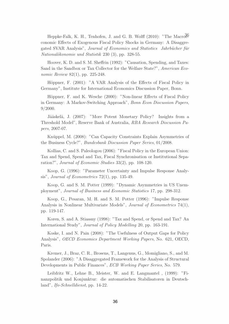
36Heppke-Falk, K. H., Tenhofen, J. and G. B. Wolff (2010): ”The Macroe-

conomic Effects of Exogenous Fiscal Policy Shocks in Germany: A Disaggre-

gated SVAR Analysis”, Journal of Economics and Statistics Jahrbucher fur

Nationalokonomie und Statistik 230 (3), pp. 328-55.

Hoover, K. D. and S. M. Sheffrin (1992): ”Causation, Spending, and Taxes:

Sand in the Sandbox or Tax Collector for the Welfare State?”, American Eco-

nomic Review 82(1), pp. 225-248.

Hoppner, F. (2001): ”A VAR Analysis of the Effects of Fiscal Policy in

Germany”, Institute for International Economics Discussion Paper, Bonn.

Hoppner, F. and K. Wesche (2000): ”Non-linear Effects of Fiscal Policy

in Germany: A Markov-Switching Approach”, Bonn Econ Discussion Papers,

9/2000.

Jaaskela, J. (2007): ”More Potent Monetary Policy? Insights from a

Threshold Model”, Reserve Bank of Australia, RBA Research Discussion Pa-

pers, 2007-07.

Knuppel, M. (2008): ”Can Capacity Constraints Explain Asymmetries of

the Business Cycle?”, Bundesbank Discussion Paper Series, 01/2008.

Kollias, C. and S. Paleologou (2006): ”Fiscal Policy in the European Union:

Tax and Spend, Spend and Tax, Fiscal Synchronisation or Institutional Sepa-

ration?”, Journal of Economic Studies 33(2), pp. 108-120.

Koop, G. (1996): ”Parameter Uncertainty and Impulse Response Analy-

sis”, Journal of Econometrics 72(1), pp. 135-49.

Koop, G. and S. M. Potter (1999): ”Dynamic Asymmetries in US Unem-

ployment”, Journal of Business and Economic Statistics 17, pp. 298-312.

Koop, G., Pesaran, M. H. and S. M. Potter (1996): ”Impulse Response

Analysis in Nonlinear Multivariate Models”, Journal of Econometrics 74(1),

pp. 119-147.

Koren, S. and A. Stiassny (1998): ”Tax and Spend, or Spend and Tax? An

International Study”, Journal of Policy Modelling 20, pp. 163-191.

Koske, I. and N. Pain (2008): ”The Usefulness of Output Gaps for Policy

Analysis”, OECD Economics Department Working Papers, No. 621, OECD,

Paris.

Kremer, J., Braz, C. R., Brosens, T., Langenus, G., Momigliano, S., and M.

Spolander (2006): ”A Disaggregated Framework for the Analysis of Structural

Developments in Public Finances”, ECB Working Paper Series, No. 579.

Leibfritz W., Lehne B., Meister, W. and E. Langmantel , (1999): ”Fi-

nanzpolitik und Konjunktur: die automatischen Stabilisatoren in Deutsch-

land”, Ifo-Schnelldienst, pp. 14-22.

36

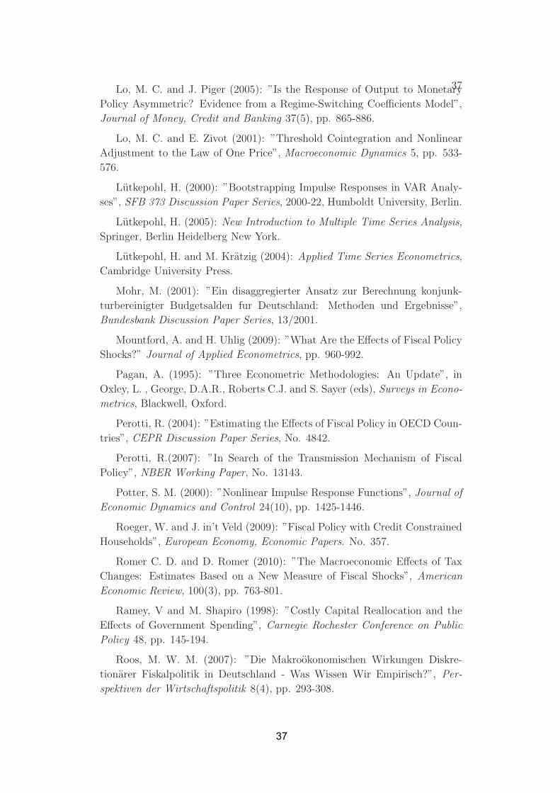
37Lo, M. C. and J. Piger (2005): ”Is the Response of Output to Monetary

Policy Asymmetric? Evidence from a Regime-Switching Coefficients Model”,

Journal of Money, Credit and Banking 37(5), pp. 865-886.

Lo, M. C. and E. Zivot (2001): ”Threshold Cointegration and Nonlinear

Adjustment to the Law of One Price”, Macroeconomic Dynamics 5, pp. 533-

576.

Lutkepohl, H. (2000): ”Bootstrapping Impulse Responses in VAR Analy-

ses”, SFB 373 Discussion Paper Series, 2000-22, Humboldt University, Berlin.

Lutkepohl, H. (2005): New Introduction to Multiple Time Series Analysis,

Springer, Berlin Heidelberg New York.

Lutkepohl, H. and M. Kratzig (2004): Applied Time Series Econometrics,

Cambridge University Press.

Mohr, M. (2001): ”Ein disaggregierter Ansatz zur Berechnung konjunk-

turbereinigter Budgetsalden fur Deutschland: Methoden und Ergebnisse”,

Bundesbank Discussion Paper Series, 13/2001.

Mountford, A. and H. Uhlig (2009): ”What Are the Effects of Fiscal Policy

Shocks?” Journal of Applied Econometrics, pp. 960-992.

Pagan, A. (1995): ”Three Econometric Methodologies: An Update”, in

Oxley, L. , George, D.A.R., Roberts C.J. and S. Sayer (eds), Surveys in Econo-

metrics, Blackwell, Oxford.

Perotti, R. (2004): ”Estimating the Effects of Fiscal Policy in OECD Coun-

tries”, CEPR Discussion Paper Series, No. 4842.

Perotti, R.(2007): ”In Search of the Transmission Mechanism of Fiscal

Policy”, NBER Working Paper, No. 13143.

Potter, S. M. (2000): ”Nonlinear Impulse Response Functions”, Journal of

Economic Dynamics and Control 24(10), pp. 1425-1446.

Roeger, W. and J. in’t Veld (2009): ”Fiscal Policy with Credit Constrained

Households”, European Economy, Economic Papers. No. 357.

Romer C. D. and D. Romer (2010): ”The Macroeconomic Effects of Tax

Changes: Estimates Based on a New Measure of Fiscal Shocks”, American

Economic Review, 100(3), pp. 763-801.

Ramey, V and M. Shapiro (1998): ”Costly Capital Reallocation and the

Effects of Government Spending”, Carnegie Rochester Conference on Public

Policy 48, pp. 145-194.

Roos, M. W. M. (2007): ”Die Makrookonomischen Wirkungen Diskre-

tionarer Fiskalpolitik in Deutschland - Was Wissen Wir Empirisch?”, Per-

spektiven der Wirtschaftspolitik 8(4), pp. 293-308.

37

38Root, T. H. and D. Lien (2003): ”Impulse Responses in a Threshold Coin-

tegrated System: the Case of Natural Gas Markets”, Applied Financial Eco-

nomics 13(1), pp. 23-35.

Spilimbergo, A., Symansky S. A. and M. Schindler (2009): Fiscal Multipli-

ers, IMF Staff Position Note No. 2009/11.

Scharnagl, M. and K.-H. Todter (2004): ”How Effective are Automatic

Stabilisers? Theory and Empirical Results for Germany and Other OECD

Countries”, Deutsche Bundesbank, Discussion Paper Series 1, No. 21.

Tong, H. (1978): ”On a threshold model”, in Chen, C. H.Pattern Recogni-

tion and Signal Processing, Sijthoff and Noordhoff, Amsterdam.

Tong, H. and K. S. Lim (1980): ”Threshold Autoregression, Limit Cycles

and Cyclical Data”, Journal of the Royal Statistical Society, Series B, 42(3),

pp. 245-292.

Tong, H. (1983): ”Threshold Models in Nonlinear Time Series Analysis”,

Springer Lecture Notes in Statistics 21, Springer, New York.

Tsay, R. S. (1998): ”Testing and Modelling Multivariate Threshold Mod-

els”, Journal of the American Statistical Association 93, pp. 1188-1202.

Noord, P. v. d. (2000): ”The Size and Role of Automatic Stabilisers in

the 1990s and Beyond”, OECD Economics Department Working Papers, No.

230, OECD, Paris.

Weise, C. L. (1999): ”The Asymmetric Effects of Monetary Policy: A

Nonlinear Vector Autoregression Approach”, Journal of Money, Credit and

Banking 31(1), pp. 85-108.

Internet: http://www.uni-mannheim.de/edz/pdf/eurostat/06/KS-DT-06-

012-EN.pdf.

38

Fig

ure

8:Low

erR

egim

e:a

1=

0.5,

2%G

row

thShock

Fig

ure

9:Low

erR

egim

e:a

1=

1.5,

2%G

row

thShock

39

Fig

ure

10:

Low

erR

egim

e:19

76-2

008

Fig

ure

11:

Upper

Reg

ime:

1976

-200

8

40

Fig

ure

12:

5%G

row

thShock

-Low

erR

egim

eFig

ure

13:

5%G

row

thShock

-U

pper

Reg

ime

41

Fig

ure

14:

IRfo

rG

DP

Gro

wth

asT

hre

shol

d:

2%G

row

th

Shock

-Low

erR

egim

e

Fig

ure

15:

IRfo

rG

DP

Gro

wth

asT

hre

shol

d:

2%G

row

th

Shock

-U

pper

Reg

ime

42

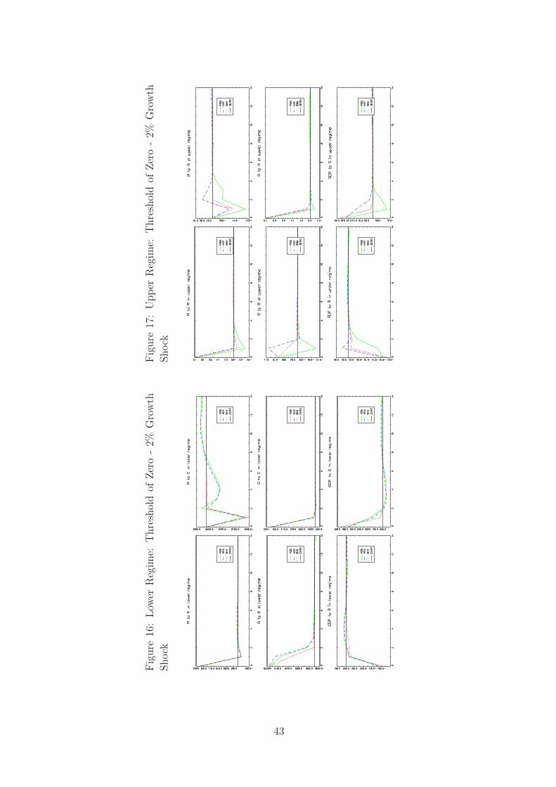
Fig

ure

16:

Low

erR

egim

e:T

hre

shol

dof

Zer

o-

2%G

row

th

Shock

Fig

ure

17:

Upper

Reg

ime:

Thre

shol

dof

Zer

o-

2%G

row

th

Shock

43

Fig

ure

18:

Low

erR

egim

e:C

hol

esky

Ord

erG

DP→

R→

GFig

ure

19:

Low

erR

egim

e:C

hol

esky

Ord

erR

→G

→G

DP

44

Fig

ure

20:

Upper

Reg

ime:

Chol

esky

Ord

erG

DP→

R→

GFig

ure

21:

Upper

Reg

ime:

Chol

esky

Ord

erR

→G

→G

DP

45

46

The following Discussion Papers have been published since 2010:

Series 1: Economic Studies

01 2010 Optimal monetary policy in a small open economy with financial frictions Rossana Merola

02 2010 Price, wage and employment response Bertola, Dabusinskas to shocks: evidence from the WDN survey Hoeberichts, Izquierdo, Kwapil Montornès, Radowski

03 2010 Exports versus FDI revisited: C. M. Buch, I. Kesternich Does finance matter? A. Lipponer, M. Schnitzer

04 2010 Heterogeneity in money holdings Ralph Setzer across euro area countries: Paul van den Noord the role of housing Guntram Wolff

05 2010 Loan supply in Germany U. Busch during the financial crises M. Scharnagl, J. Scheithauer

06 2010 Empirical simultaneous confidence Òscar Jordà, Malte Knüppel regions for path-forecasts Massimiliano Marcellino

07 2010 Monetary policy, housing booms Sandra Eickmeier and financial (im)balances Boris Hofmann

08 2010 On the nonlinear influence of Stefan Reitz Reserve Bank of Australia Jan C. Ruelke interventions on exchange rates Mark P. Taylor

09 2010 Banking and sovereign risk S. Gerlach in the euro area A. Schulz, G. B. Wolff

10 2010 Trend and cycle features in German residential investment before and after reunification Thomas A. Knetsch

47

11 2010 What can EMU countries’ sovereign bond spreads tell us about market perceptions of default probabilities Niko Dötz during the recent financial crisis? Christoph Fischer

12 2010 User costs of housing when households face Tobias Dümmler a credit constraint – evidence for Germany Stephan Kienle

13 2010 Extraordinary measures in extraordinary times – public measures in support of the financial Stéphanie Marie Stolz sector in the EU and the United States Michael Wedow

14 2010 The discontinuous integration of Western Europe’s heterogeneous market for corporate control from 1995 to 2007 Rainer Frey

15 2010 Bubbles and incentives: Ulf von Kalckreuth a post-mortem of the Neuer Markt in Germany Leonid Silbermann

16 2010 Rapid demographic change and the allocation of public education resources: evidence from East Germany Gerhard Kempkes

17 2010 The determinants of cross-border bank flows to emerging markets – new empirical evidence Sabine Herrmann on the spread of financial crisis Dubravko Mihaljek

18 2010 Government expenditures and unemployment: Eric Mayer, Stéphane Moyen a DSGE perspective Nikolai Stähler

19 2010 NAIRU estimates for Germany: new evidence on the inflation-unemployment trade-off Florian Kajuth

20 2010 Macroeconomic factors and Claudia M. Buch micro-level bank risk Sandra Eickmeier, Esteban Prieto

48

21 2010 How useful is the carry-over effect for short-term economic forecasting? Karl-Heinz Tödter

22 2010 Deep habits and the macroeconomic effects of government debt Rym Aloui

23 2010 Price-level targeting C. Gerberding when there is price-level drift R. Gerke, F. Hammermann

24 2010 The home bias in equities P. Harms and distribution costs M. Hoffmann, C. Ortseifer

25 2010 Instability and indeterminacy in Michael Krause a simple search and matching model Thomas Lubik

26 2010 Toward a Taylor rule for fiscal policy M. Kliem, A. Kriwoluzky

27 2010 Forecast uncertainty and the Bank of England interest rate decisions Guido Schultefrankenfeld

01 2011 Long-run growth expectations M. Hoffmann and “global imbalances” M. Krause, T. Laubach

02 2011 Robust monetary policy in a New Keynesian model with imperfect Rafael Gerke interest rate pass-through Felix Hammermann

03 2011 The impact of fiscal policy on economic activity over the business cycle – Anja Baum evidence from a threshold VAR analysis Gerrit B. Koester

49

Series 2: Banking and Financial Studies

01 2010 Deriving the term structure of banking Stefan Eichler crisis risk with a compound option Alexander Karmann approach: the case of Kazakhstan Dominik Maltritz

02 2010 Recovery determinants of distressed banks: Thomas Kick Regulators, market discipline, Michael Koetter or the environment? Tigran Poghosyan

03 2010 Purchase and redemption decisions of mutual Stephan Jank fund investors and the role of fund families Michael Wedow

04 2010 What drives portfolio investments of German banks in emerging capital markets? Christian Wildmann

05 2010 Bank liquidity creation and Berger, Bouwman risk taking during distress Kick, Schaeck

06 2010 Performance and regulatory effects of non-compliant loans in German synthetic mortgage-backed securities transactions Gaby Trinkaus

07 2010 Banks’ exposure to interest rate risk, their earnings from term transformation, and the dynamics of the term structure Christoph Memmel

08 2010 Completeness, interconnectedness and distribution of interbank exposures – a parameterized analysis of the stability of financial networks Angelika Sachs

09 2010 Do banks benefit from internationalization? C. M. Buch Revisiting the market power-risk nexus C. Tahmee Koch, M. Koetter

50

10 2010 Do specialization benefits outweigh Rolf Böve concentration risks in credit portfolios Klaus Düllmann of German banks? Andreas Pfingsten

11 2010 Are there disadvantaged clienteles in mutual funds? Stephan Jank

12 2010 Interbank tiering and money center banks Ben Craig, Goetz von Peter

13 2010 Are banks using hidden reserves Sven Bornemann, Thomas Kick to beat earnings benchmarks? Christoph Memmel Evidence from Germany Andreas Pfingsten

14 2010 How correlated are changes in banks’ net interest income and in their present value? Christoph Memmel

01 2011 Contingent capital to strengthen the private safety net for financial institutions: Cocos to the rescue? George M. von Furstenberg

02 2011 Gauging the impact of a low-interest rate Anke Kablau environment on German life insurers Michael Wedow

03 2011 Do capital buffers mitigate volatility Frank Heid of bank lending? A simulation study Ulrich Krüger

04 2011 The price impact of lending relationships Ingrid Stein

51

Visiting researcher at the Deutsche Bundesbank

The Deutsche Bundesbank in Frankfurt is looking for a visiting researcher. Among others under certain conditions visiting researchers have access to a wide range of data in the Bundesbank. They include micro data on firms and banks not available in the public. Visitors should prepare a research project during their stay at the Bundesbank. Candidates must hold a PhD and be engaged in the field of either macroeconomics and monetary economics, financial markets or international economics. Proposed research projects should be from these fields. The visiting term will be from 3 to 6 months. Salary is commensurate with experience. Applicants are requested to send a CV, copies of recent papers, letters of reference and a proposal for a research project to: Deutsche Bundesbank Personalabteilung Wilhelm-Epstein-Str. 14 60431 Frankfurt GERMANY