THE IMPACT OF FINANCIAL REFORMS ON MONEY DEMAND · PDF filestock market as banks raised their...
82
THE IMPACT OF FINANCIAL REFORMS ON MONEY DEMAND AND ECONOMIC GROWTH IN NIGERIA BY ANUMNU CLARA CHIALUKA PG/MSC/12/61860 AN M.SC PROPOSAL SUBMITTED TO THE DEPARTMENT OF ECONOMICS, FACULTY OF THE SOCIAL SCIENCES, UNIVERSITY OF NIGERIA NSUKKA, ENUGU STATE. SUPERVISOR PROF. (MRS.) S.I. MADUEME NOVEMBER, 2014
Transcript of THE IMPACT OF FINANCIAL REFORMS ON MONEY DEMAND · PDF filestock market as banks raised their...
i
THE IMPACT OF FINANCIAL REFORMS ON MONEY DEMAND AND
ECONOMIC GROWTH IN NIGERIA
BY
ANUMNU CLARA CHIALUKA
PG/MSC/12/61860
AN M.SC PROPOSAL SUBMITTED TO THE DEPARTMENT OF ECONOMICS,
FACULTY OF THE SOCIAL SCIENCES, UNIVERSITY OF NIGERIA NSUKKA, ENUGU
STATE.
SUPERVISOR PROF. (MRS.) S.I. MADUEME
NOVEMBER, 2014
i
TITLE PAGE
THE IMPACT OF FINANCIAL REFORMS ON MONEY DEMAND AND ECONOMIC
GROWTH IN NIGERIA
i
ii
CERTIFICATION
This is to certify that Anumnu Clara Chialuka, an M.Sc student of the University of Nigeria, Nsukka
with registration number PG/MSC/12/61860 has successfully completed the research required for the
Award of Master of Science degree in Economics, University of Nigeria Nsukka, Enugu State.
PROF. (MRS) S.I. MADUEME PROF. C. C. AGU
Supervisor Head of Department
iii
APPROVAL PAGE
This research work titled: ―The Impact of Financial Reforms on Money Demand and Economic
Growth in Nigeria‖ has followed due process and has been approved to have met the minimum
requirements for the award of the Master of Science Degree in the Department of Economics,
University of Nigeria, Nsukka.
PROF. (MRS) S.I. MADUEME PROF. C. C. AGU
Supervisor Head of Department
PROF. I. A. MADU
Dean, Faculty of Social sciences External Examiner

iv
DEDICATION
This research work is dedicated to Almighty God my creator who is the fount of all wisdom and
knowledge

v
ACKNOWLEDGMENTS
I must in the first instance express my endless and sincere gratitude and thanks to God Almighty for
giving me strength, will, power and wisdom during the process of conducting this research work, may
His name alone be praised forever, Amen.
A well deserved appreciation goes to my project supervisor Prof. S.I. Madueme whose kindness,
attention and co-operation during the research are immeasurable.
My profound gratitude goes to my brother Justin for his encouragement and the challenges he gave
me acted as propelling force towards the rounding up of this work. Also to friends who in one way or
the order contributed to the success of this work.
Lastly but very important my love to my family for their great support, financially and morally.
I thank you all and pray for God‘s continued guidance and protection.
vi
Table of Content Title Page ............................................................................................................. Error! Bookmark not defined.
Certification Page ................................................................................................ Error! Bookmark not defined.
Approval Page...................................................................................................... Error! Bookmark not defined.
Dedication ............................................................................................................ Error! Bookmark not defined.
Acknowledgement ............................................................................................... Error! Bookmark not defined.
Table of Content .................................................................................................................................................. vi
CHAPTER ONE ................................................................................................................................................... 1
INTRODUCTION ................................................................................................................................................ 1
1.1 Background of the Study ................................................................................................................................ 1
1.2 Statement of Problems .................................................................................................................................... 4
1.3 Research Questions ......................................................................................................................................... 6
1.4 Objectives of the Study ................................................................................................................................... 6
1.5 Research Hypotheses ...................................................................................................................................... 6
1.6 Scope of the Study ....................................................................................................................................... 6
1.7 Significance of the Study ................................................................................................................................ 7
LITERATURE REVIEW ..................................................................................................................................... 8
2.1 Conceptual Framework ................................................................................................................................... 8
2.2 Theoretical Literature ................................................................................................................................... 10
2.2.1Theory on Financial Reforms ................................................................................................................. 10
2.2.2 Theory on Money Demand .................................................................................................................... 12
2.2.2.1 Keynesian Liquidity Preference Theory ............................................................................................. 12
2.2.3 Post-Keynes Theory ............................................................................................................................... 14
2.2.4 Classical Theories .................................................................................................................................. 14
2.3 Empirical Literature on Financial Reforms and Demand for Money ........................................................... 17
2.3.1Review of Foreign Studies ...................................................................................................................... 17
2.3.2 Review of Domestic Studies .................................................................................................................. 21
2.4 Limitations of Previous Studies .................................................................................................................... 27
CHAPTER THREE ........................................................................................................................................ 31
RESEARCH METHODOLOGY ....................................................................................................................... 31
3.1 Theoretical Framework ................................................................................................................................. 31
3.2 Model Specification ...................................................................................................................................... 32
3.2.1 Financial reform and Money Demand ................................................................................................ 32
vii
3.2.2Financial Reform and Economic Growth ............................................................................................... 34
3.3 Estimation Procedure .................................................................................................................................... 35
3.3.1 Unit Root Test ............................................................................................................................................ 37
3.4 Justification of the Model ............................................................................................................................. 38
3.5 Preliminary tests on variables of the study ................................................................................................... 38
3.5.1 Testing for normality ............................................................................................................................. 39
3.5.2 Testing for stationarity ........................................................................................................................... 39
3.5.3 Testing for serial correlation. ................................................................................................................. 40
3.6 Data and Sources .......................................................................................................................................... 41
3.7 Econometric Software ................................................................................................................................... 41
4.1 Introduction ......................................................................................................................................... 42
4.2 Unit root tests and the order of integration. .................................................................................... 42
4.3 Correction of non-stationarity ........................................................................................................ 43
4.4 Testing for co integration using the engel-granger residual approach. ......................................... 43
4.5 Money Demand and financial reform ........................................................................................... 44
4.6 Error correction model (ECM) for the impact of financial reform on money demand. ............... 45
4.7 Diagnostic tests ............................................................................................................................ 47
4.8 The short term dynamics of economic growth ................................................................................. 48
4.9 Diagnostic tests ............................................................................................................................. 50
CHAPTER FIVE ................................................................................................................................................ 51
SUMMARY OF THE FINDINGS, CONCLUSIONS AND RECOMENDATIONS ........................................ 51
5.1 Summary of the findings ......................................................................................................................... 51
5.2 Recommendations ................................................................................................................................... 51
5.3 Conclusions ................................................................................................................................................... 53
5.4 Areas for further study ............................................................................................................................ 55
REFERENCES ................................................................................................................................................... 56
APPENDICES…………………………………………………………………………………..……………..62
viii
ABSTRACT
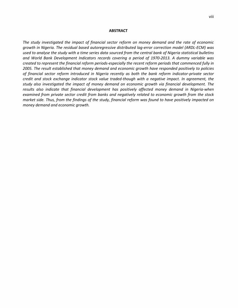
The study investigated the impact of financial sector reform on money demand and the rate of economic growth in Nigeria. The residual based autoregressive distributed lag-error correction model (ARDL-ECM) was used to analyse the study with a time series data sourced from the central bank of Nigeria statistical bulletins and World Bank Development Indicators records covering a period of 1970-2013. A dummy variable was created to represent the financial reform periods-especially the recent reform periods that commenced fully in 2005. The result established that money demand and economic growth have responded positively to policies of financial sector reform introduced in Nigeria recently as both the bank reform indicator-private sector credit and stock exchange indicator stock value traded-though with a negative impact. In agreement, the study also investigated the impact of money demand on economic growth via financial development. The results also indicate that financial development has positively affected money demand in Nigeria-when examined from private sector credit from banks and negatively related to economic growth from the stock market side. Thus, from the findings of the study, financial reform was found to have positively impacted on money demand and economic growth.
1
CHAPTER ONE
INTRODUCTION
1.1 Background of the Study
The rising importance of the financial sector in the economic development of countries especially
developing countries, as well as the rapid rate of innovation in the sector has generated growing
research interest in financial policy changes. The Nigerian financial system is one of the largest and
most diversified in Sub-Saharan Africa (Afangideh, 2010). The system became liberalized when the
structural adjustment programme was introduced in 1986. In recent years, the system had undergone
significant changes in terms of the policy environment, number of institutions, ownership structure,
depth and breadth of markets, as well as in the regulatory framework.
The financial reforms which began in 2004 with the consolidation programme were necessitated by
the need to strengthen the banks and financial sector in general. The policy thrust at inception, was to
grow the banks and position them to play pivotal roles in driving development across the sectors of
the economy. As a result, banks were consolidated through mergers and acquisitions, raising the
capital base from N2 billion to a minimum of N25 billion, which reduced the number of banks from
89 to 25 in 2005, and later to 24. However, this led to the expanded use of branches by existing and
new banks. The expansion of branch banking in Nigeria has occurred with the development of new
technologies to deliver financial services, such as Automated Teller Machines (ATMs) and other
stored value cards. These cost effective innovations and products that have become available, have
the purpose of reducing the pressure on over-the-counter services to bank customers.
It is important to note that the recapitalisation and merging of some banks affected dealings in the
stock market as banks raised their required minimum capital through the capital market by issuing
new securities. Beyond the need to recapitalize the banks, the regulatory reforms also focused on the
2
following: risk-focused and rule-based regulatory framework, zero tolerance in regulatory framework
in data/information rendition/reporting and infractions; strict enforcement of corporate governance
principles in banking; expeditious process for rendition of returns by banks and other financial
institutions through Electronic Flight Assistance (e-FASS); as well as the introduction of a flexible
interest rate based framework that made the monetary policy rate the operating target. The new
framework has enabled the banking sector to be proactive in countering inflationary pressures and has
helped to check wide fluctuations in the interbank rates and also engendered orderly development of
the money market segment and payments system reforms, among others. Moreover, in 2010, the
Asset Management Corporation of Nigeria (AMCON) was established following the promulgation of
its enabling Act by the National Assembly. It is a special purpose vehicle aimed at addressing the
problem of non-performing loans in the Nigerian banking industry, among others. And in 2011, the
financial sector introduced a new policy ―Cash less Policy‖ as part of ongoing reforms to address
currency management challenges in Nigeria, as well as enhance the national payments system.
However, one crucial question that needs to be addressed is whether these financial reforms have led
to an improvement in the allocation of resources or not, since proper allocation of resources leads to
high real output. Economic theory tells us that financial reforms foster economic growth; empirical
works so far have not found evidence for the existence of such a link. While some countries have
benefited from tools of financial reforms others have not enjoyed higher economic growth. Some
have even experienced serious crises and recessions in those years, following (Fratzscher and
Bussiere, 2004). The impact of financial reforms on macroeconomic performance is very important
for relatively developing countries like Nigeria, empirical evidence from World Bank (2012) and
CBN (2012) reveals that from 1986 to 2012, macroeconomic outcomes in Nigeria such as growth
rate, real interest rate and inflation were among the most affected. The rate of growth in Nigeria was
3
3% in 1986 during financial liberalization but declined to -1% in 1987 and thereafter soared to 10%
in 1988. It further declined to 7% in 1989 and rose again to 8% in 1990. From 1990 to 1994, there
was a continuous decline reaching as low as 1.3% in 1994. There was a little improvement between
1995 and 1996 when the economy grew from 2% to 4%, but it began to decline again from 3% in
1997 to 1% in 1999, the very year Nigeria embraced a new democratic leadership. Owing to some
policy initiatives, the economy improved to 5% in 2000 but declined again to 3% and 2% in 2001 and
2002 respectively. However, when the CBN implemented the recapitalization policy the GDP growth
was short-lived as the economy nosedived again to 5% in 2005 but increased minimally to 6%
between 2006 and 2008.The economy experienced another growth between 2009 and 2010 at 7% and
8% respectively but declined again to 7% in 2011. These fluctuations in growth rates of the economy
have been attributed to many factors ranging from economic mismanagement to erratic financial
policy reversals.
Moreover, the stability of money demand function was at the centre of monetarist claims that
financial reforms should be the backbone of a non-inflationary policy stance (Ighodaro & Ihaza
2008). Starting with Poole (1988) and Lucas (1988), there is a growing consensus that long run
money demand is stable. This view is supported by the findings of a cointegrating relation among real
M1, interest rates and output (Hoffman and Rasche, 1991 and Stock & Watson 1993). Generally, the
stability of the demand for money function has profound implications for the conduct of monetary
policy particularly in this era of economic/financial reforms in Nigeria. Meanwhile, Gbadebo, (2010),
is of the view that the search for a stable demand for money has been a very contentious issue
between the Keynesians and Monetarists of the 1960s and 1970s, as no model on the demand for
money set forth by any of these two schools as well as their contemporaries has withstood the test of
time. He further stated that the instability of the demand for money in the 1970s and in the 1980s has
4
been attributed primarily to changes in the performance of financial markets in the area of new
financial products arising out of financial policy changes.
Meanwhile, the use of monetary policy as a tool for macro-economic stabilization depends largely on
the behaviour of the demand for money or real cash balances in the hands of economic agents. This
brings in the demand for money function which expresses a mathematical relationship between the
quantity of money demanded and its various determinants; interest rate, income, price level, credit
availability, frequency of payments etc. The stability of these relationships is vital in determining the
appropriateness and effectiveness of the tools or instruments of monetary policy. In recent times the
instability of the previously stable demand for money function has thrown up new studies at its
various determinants and several other fronts have been explored by economists and econometricians
alike, (Busari, 2005). One of these fronts is financial policy reforms which has blurred the distinction
between M1 and other assets. Earlier on Miller, (1986) posited that it has blurred the various
definitions of money – M1, M2, M3 etc. In Nigeria, it has begun to hit home with the recent
recapitalization of the banking sector, with the banks now bringing in new financial products that
have combinations of savings features, higher interest earnings, easy withdrawals and transfers, with
increasingly close substitutes for money being introduced by the day, good news for customers but a
hellish nightmare for monetary authorities, (Busari 2005).
1.2 Statement of Problems
Nigerian economy had gone through several financial reforms in the last ten years, including
facilitating the new entry of many domestic banks, N25billion recapitalization of commercial banks,
the gradual deregulation of lending deposit interest rate; facilitating the use of updating payment
technologies like ATM and electronic transfer of deposits. Also included in this reform are, the
5
expansion of a variety of internet banking service like e-banking and mobile banking technology,
enhancement of telecommunication infrastructure, and many others. While these fast financial
developments could promote economic growth, such developments may also hamper the
effectiveness of monetary policy, (Sanya, 2013). For instance, financial development and the
proliferation of these new financial products and deposit substitutes could cause instability in the
underlying money demand relationship with important consequences for the conduct and efficacy of
monetary policy. These developments may have altered the relationship between money, income,
prices and other key economic variables, and may have caused the money demand function to
become structurally unstable (Gbadebo and Okunrinboye, 2009).Kumar et al (2012) has already
submitted that previous reform exercises, especially that of SAP, caused the country a serious
turbulence. They supported their argument with the submission of Anorou (2002) who tested for the
stability of the demand for M2 around the SAP period using quarterly data between 1986 (Q2) and
2000(Q1); the principal result was an unreasonably high estimate of 5.70 for the elasticity of demand.
In addition, Sanya (2013) stated that the recent upgrade the Nigerian financial institutions to global
standards may have implications on the money demand function. Thus, shocks in the global financial
scene and large capital inflows altered the money demand function, making the relationship between
monetary aggregates and output as well as prices less stable as experienced during the last global
financial crisis.
It has also been discovered by researchers (Gurley & Shaw, 1995; Darrat, 2010) that the emergence
of new interest bearing money substitute resulting from financial reforms may unexpectedly increase
the interest rate sensitivity of money holdings. Such elasticity shift in the money demand relations
could weaken the presumed stable relations between monetary aggregates and ultimate policy
objectives of price stability. If this arises, it casts serious doubt on time efficacy of monetary policy.
6
Thus, this study examines the impacts of the changing structure of Nigerian financial system on
money demand and the economic growth performance. More specifically, the study investigates
whether financial markets and stock market development are mutually reinforcing or not in
promoting economic growth and money demand in Nigeria.
1.3 Research Questions
(i) Do post-SAP financial sector reforms have significant effect on money demand in Nigeria?
(ii) Has post-SAP financial sector reforms impacted on the economic growth in Nigeria?
1.4 Objectives of the Study
The broad objective of this study is to examine the effect of financial reform on money demand and
economic growth in Nigeria. The specific objectives of this study include:
(i) To examine the effect of post-SAP financial sector reforms on money demand.
(ii) To investigate the effect of post-SAP financial sector reforms on economic growth.
1.5 Research Hypotheses
H01: Post-SAP financial reform indicators have no effect on money demand in Nigeria.
HA1: Post-SAP financial reform indicators have an effect on money demand in Nigeria.
H02: Post-SAP financial reform indicators have no effect on economic growth in Nigeria.
HA2: Post-SAP financial reform indicators have an effect on economic growth in Nigeria.
1.6 Scope of the Study
The study is a country specific study focusing on the financial sector of the Nigerian economy using
time series data covering the period 1970 to 2013. It has two models with the first model addressing
7
the impact of financial reform indicators on money demand and the second model addressing the
impact of financial reform indicators on GDP. Real GDP, consumer price index (CPI), stock market
value traded, private sector credit (PSC) will be used as proximate variables for performance of the
banking sector and will be expressed in the models as exogenous variables, while the natural log of
broad money demand (represented by M2) will be used as proximate variable to capture money
demand and will be expressed in the models as endogenous variable. FRD which represent financial
sector reform dummy will take the value 0 for period before 2004 and 1 for period after 2004.
1.7 Significance of the Study
It is important to know if money demand function has been unstable as a result of the recent financial
sector reforms. Knowing this is vital in order to establish the relationship between interest rates and
aggregate expenditure as this is important for choosing instruments for conducting monetary policy.
If the demand for money is significantly affected, then the case for conducting macro-economic
stabilization by regulating the growth of the money supply and interest rate changes may be seriously
threatened. Thus, from the findings of this study, knowledge of the extent to which the financial
sector reform policy has impacted on money demand and economic growth in Nigeria will be of great
interest to both the policy makers, monetary authorities and other researchers.
8
CHAPTER TWO
LITERATURE REVIEW
2.1 Conceptual Framework
Financial Reform
Financial sector reform refers to the process to liberalise the financial sector of a country with an aim
to create favourable environment to increase the money demand in the economy. This is assumed to
take place in two ways;
(i) By increasing the financial resources to lead the supply-induced demand for money.
(ii) By creating the enabling environment for investments in the economy.
For Nnanna and Dogo (1998) the concept of financial reform is usually employed to explain a state of an
atomized financial system (i.e.) a financial system which is largely free from financial repression.
According to Fisher (2001), financial reform refers to the greater financial resource mobilization in the
formal financial sector and the ease in liquidity constraints of banks and enlargement of funds available
to finance projects.
There are many different ways in which the financial sector can be said to be reformed. For example;(a)
the efficiency and competitiveness of the sector may improve (b) the range of financial services that are
available may increase (c) the diversity of institutions which operate in the financial sector may increase,
(d) the amount of money that is intermediated through the financial sector may increase,(e) the extent to
which capital is allocated by private sector financial institutions to private sector enterprises responding
to market signals may increase,(f) the regulation and stability of the financial sector may improve and (e)
particularly important from the welfare perspective more of the population may gain access to financial
services, (Department for International Development, 2004).
9
Economic activities in the country can be greatly facilitated by modern banking services. Financial
reform involves the introduction and intensive use of new financial products. In this context, it is
aimed at modernizing the banking system in order to avail modern banking and financial services in
the Nigerian financial market.
Money Demand
In addition, defining the money demand function is a central concern for monetary policy authority
because the combination of money supply and money demand determines interest rates, and therefore
affects the goals of monetary policy. Thus, by definition, demand for money is the quantity of money
people are willing to hold at a given interest rate. In other words, the preference to hold their cash
balances instead of assets. This is referred to as the liquidity preference, (Aiyedogbon, Ibeh,
Ohwofasa, 2013). A stable money demand allows for better prediction of the effects of monetary
policy on interest rates, output, and inflation, and therefore reduces the possibility of an inflation bias
(Cziraky & Gillman, 2006). Stable money demand is a precondition for an effective monetary policy,
especially for countries pursuing a monetary targeting framework. This monetary policy focuses on
the relationship between the rates of interest in an economy, which is the price at which money can be
borrowed and the total supply of money. Monetary policy uses a variety of instruments to control one
or both of these, to influence outcomes like economic growth, inflation, exchange rates with other
currencies and unemployment. Where currency is under a monopoly of issuance, or where there is a
regulated system of issuing currency through banks which are tied to a Central Bank, the monetary
authority has the ability to alter the money supply and thus influence the interest rate to achieve
policy goals.
10
2.2 Theoretical Literature
2.2.1Theory on Financial Reforms
The intellectual framework for financial reforms in developing countries in the 1980s was provided by
the works of Mckinnon (1973) and Shaw (1973). The Mckinnon-Shaw (M-S) paradigm contained two
essential issues; (1) the financial sector is critical for economic growth and (2) extensive government
controls imposed on the financial sector prevents financial deepening and impedes the contribution of the
sector to development. The first issue was not all that new, but only reiterated and re-affirmed ideas
contained in the works of earlier writers such as Gurley and Shaw (1955), Patrick (1966) and Goldsmith
(1969). The second issue was innovative, with the M-S thesis systematically detailing the efficiency and
output costs associated with direct state intervention in the financial system labelled ―financial
repression‖. Goldsmith (1969), McKinnon (1973) and Shaw (1973) present their views by saying that the
poor performance of most developing economies is due to interest rate ceilings, high reserve
requirements, and quantitative restrictions in the credit allocation mechanism caused by financial
repression leading to low savings, credit rationings and low investments. In contrast, some of the works
have either ignored or opposed the financial development, for example; Arestis (2005) evaluated the
Financial Liberalisation in the lights of the relationship between financial development and growth and
clearly mentioned that no convincing empirical evidence was found to support the proposition of the
financial liberalisation hypothesis.
However, the general notion from their debate is that the functions of financial institutions in the savings-
investment process were spelt out as being an effective element for the mobilization and allocation of
capital by equilibrating the supply of loan-able funds with the demand for investment funds and the
transformation and distribution of risks and maturities.
11
Pagano (1993), Jappelli and Pagano (1994) suggest that financial intermediaries can contribute
positively to the growth of the economy only if the economic environment is favourable. King and
Levine (1993) argue that government intervention in the financial system has negative effect on the
equilibrium growth rate.
However, most of the literature on the impact of financial intermediation on economic growth points
to causation running from financial intermediaries. However, Patrick (1966) argues that causation is
bidirectional: financial intermediation is both supply-leading and demand-following, that is the
setting up of financial intermediaries enhances economic growth and it may, itself be enhanced by the
existence of stable economic growth. The ―supply-leading hypothesis‖ postulates a causal
relationship from financial development to economic growth, which means deliberate creation of
financial institutions and markets that increases the supply of financial services and thus leads to real
economic growth. Recent contributors in the new economic growth literature have considered the role
of financial structure and system; this presupposes that the level of money stock drives economic
growth Agu (2008). Numerous theoretical and empirical writings on this subject have shown that
financial development is important and causes economic growth. McKinnon (1973), King and Levine
(1993), all support the supply-leading phenomenon. On the other hand, the ―demand-following
hypothesis‖ postulates a causal relationship from economic growth to financial development. Here,
an increasing demand for financial services might induce an expansion in the financial sector as the
real economy grows (i.e. financial sector responds passively to economic growth), (Gold Smith 1969)
supports this hypothesis as well.
However, the arguments in favour of incorporating a role for financial innovation or technological
change in the demand for money has long been considered in the money demand literature (Arrau, De
Gregorio, Reinhart and Wickham 1995). The demand for money is considered a function of the
12
prevailing institutional and technological framework and thus sensitive to changes in these underlying
forces. The quantity of money demanded in any economy and indeed, the set of assets that have
monetary status is dependent upon the prevailing institutions, regulations, and technology,
(McCallum and Goodfriend, 1987).
2.2.2 Theory on Money Demand
The theoretical underpinnings of the demand for money have been well established in the economic
literature with widespread agreement that the demand for money is primarily determined by real cash
balances.
2.2.2.1 Keynesian Liquidity Preference Theory
Keynes (1936) built upon the Cambridge approach to provide a more rigorous analysis of money
demand, focusing on the motives of holding money. Keynes postulated three motives for holding
money: transactions, precautionary and speculative purposes. He also formally introduced the interest
rate as another explanatory variable in influencing the demand for real balances. The main
proposition of the Keynesian analysis is that when interest rates are low, economic agents will expect
a future increase in interest rates; thus, preferring to hold whatever amount of money is supplied.
Therefore, the aggregate demand for money becomes perfectly elastic with respect to the interest rate
(liquidity trap).
However, following the emergence of liquidity preference theory, several authors have questioned
Keynes‘s rationale for a speculative demand for money and have contributed to the theoretical
literature by distinguishing broadly between the transactions demand.
13
Laidler (1977) points out that Keynes did not regard the demand for money arising from the
transactions and precautionary motives as technically fixed in their relationships with the level of
income and therefore emphasizes that the most important innovation in Keynes‘ analysis is his
speculative demand for money. The primary result of the Keynesian speculative theory is that there is
a negative relationship between money demand and the rate of interest. That is, in a period of high
interest rate, people hold less cash and probably make more savings.
Friedman (1959) opposes the Keynesian view that money does not matter and presented the quantity
theory as a theory of money demand. He modelled money as an abstract purchasing power (meaning
that people hold it with the intention of using it for upcoming purchases of goods and services)
integrated in an asset and transactions theory of money demand set within the context of neoclassical
consumer and producer behaviour microeconomic theory. Friedman argued that the velocity of
money is highly predictable and that the demand for money function is highly stable and insensitive
to interest rates. This implies that the quantity of money demanded can be predicted accurately by the
money demand function.
Chuku (2009) argues that the economic environment that guided monetary policy before 1986 was
characterized by the dominance of the oil sector, the expanding role of the public sector in the
economy and over-dependence on the external sector. In order to maintain price stability and a
healthy balance of payments position, monetary management depended on the use of direct monetary
instruments such as credit ceilings, selective credit controls, administered interest and exchange rates,
as well as the prescription of cash reserve requirements and special deposits.
Al-Samara (2011) opines that the analysis of money demand function is regarded as a key factor in
conducting reliable strategy of monetary policy and selecting the suitable nominal anchor that
monetary policy makers use to tie down the price level. The marvellous strides in monetary analysis
14
showed why a nominal anchor, such as the inflation rate, an exchange rate, or the money supply, is
such a crucial element in achieving the price stability. Continuing further, Al-Samara (2011)
emphasizes that the choice of the intermediate target in the monetary policy strategy is one of the
principal purposes of the Central Banks.
2.2.3 Post-Keynes Theory
Following Keynes, a number of models were developed to confirm the relationship between the
demand for real money, income and interest rates. These models can be classified into three separate
frameworks, namely transactions, assets and consumer demand theories of money.
Under the transactions theory of money demand framework, the inventory-theoretic approach by
(Baumol 1952) and (Tobin 1956) and the precautionary demand for money of (Cuthbertson and
Barlow, 1991) models were introduced. These models were derived from the medium-of-exchange
function of money.
The asset function of money led to the asset or portfolio approach where major emphasis is placed on
risk and expected returns of assets (Tobin, 1956).
Alternatively, the consumer demand theory approach (Friedman, 1959 and Barnett, 1980) considers
the demand for money as a direct extension of the traditional theory of demand for any durable
goods.
2.2.4 Classical Theories
According to classical economists, money acts as a numéraire. In other words, it is a commodity
whose unit is used in order to express prices and values, but whose own value remains unaffected by
this role (Sriram, 1999). However, money is deemed neutral with no real economic consequences
since its role as a store of value, is limited under the classical assumption of perfect information and
15
negligible transaction costs (Sriram, 1999). The concept of money demand took formal shape through
the quantity theory developed in the classical equilibrium framework by two different but equivalent
expressions.
Fisher (1911) provided the famous equation of exchange (MsVt =PtT), where Ms is quantity of
money, Vt is the transactions velocity of circulation, Pt is prices and T the volume of transactions)
where money is held simply to facilitate transactions and has no intrinsic value.
However, the alternative paradigm, the Cambridge approach, was primarily associated with the neo-
classical economists. This approach stressed the demand for money as public demand for money
holdings, especially the demand for real balances, which was an important factor in determining the
equilibrium price level consistent with a given quantity of money (Sriram, 1999).
Growth Theories
The Harrod Domar Model
In theory, the Harrod-Domar model is a cross between the classical and the Keynesian theories of
growth. Harrod-Domar opined that economic growth is achieved when more investment leads to
more growth. The model creates demand but it also creates capacity (Baldwin 1972). Whereas the
Keynesians concentrated only upon the former, the classicists emphasized the latter. The variables
chosen by Harrod and Domar are the broad aggregates, e.g. investment, capital and output. The model
is an early attempt to show that growth is directly related to savings and indirectly related to the
capital/output ratio (Odularu, 2008). The theory is based on linear production function with output
given by capital stock ( ) times a constant. Investment according to the theory generates income and
also augments the productive capacity of the economy by increasing the capital stock. In as much as
there is net investment, real income and output continue to expand. And, for full employment
16
equilibrium level of income and output to be maintained, both real income and output should expand
at the same rate with the productive capacity of the capital stock (Atoyebi, Akinde, Adekunjo and
Femi, 2012)
The theory maintained that for the economy to achieve a full employment, in the long run, net
investment must increase continuously as well as growth in the real income at a rate sufficient enough
to maintain full capacity use of a growing stock of capital. This implies that a net addition to the
capital stock in the form of new investment will go a long way to increase the flow of national
income. From the theory, the national savings ratio is assumed to be a fixed proportions of national
output and that total investment is determined by the level of total savings (i.e ) which must
be equal to net investment I.
Solow's Neo-classical Theory
Following the seminal contributions of Solow (1956, 1957) and Swan (1956), the neoclassical model
became the dominant approach to the analysis of growth, at least within academia. Between 1956 and
1970 economists refined ‗old growth theory‘, better known as the Solow neoclassical model of
economic growth (Solow, 2000, 2002). Building on a neoclassical production function framework,
the Solow model highlights the impact on growth of saving, population growth and technological
progress in a closed economy setting without a government sector. Despite recent developments in
endogenous growth theory, the Solow model remains the essential starting point to any discussion of
economic growth. As Mankiw (1995, 2003) notes, whenever practical macroeconomists have to
answer questions about long-run growth they usually begin with a simple neoclassical growth model
(Abel and Bernanke, 2001); (Jones, 2001a); (Barro and Sala-i-Martin, 2003).
17
The Solow theory believes that a sustained increase in capital investment increases the growth rate
only temporarily: because the ratio of capital to labour goes up (i.e. there is more capital available for
each worker to use). However, the marginal product of additional units of capital is assumed to
decline and thus an economy eventually moves back to a long-term growth path, with real GDP
growing at the same rate as the growth of the workforce plus a factor to reflect improving
productivity. The Solow Growth Model is the most famous neoclassical growth model and it is the
most common starting point for any analysis of growth in a country. It treats technological growth as
well as the rate of savings in a country as exogenous (i.e., determined outside the system). It features
both labour and capital as the factors of production, and assumes constant returns to scale (CRS) in
both factors. This is an important assumption; it means that if capital and labour are doubled as
inputs, output will also double. The Solow model is a dynamic model that predicts convergence in the
long run to a steady state rate of growth for a country (Huggett, 2013).
2.3 Empirical Literature on Financial Reforms and Demand for Money
2.3.1Review of Foreign Studies
Bhatia and Khatkhate (1975) examined the relationship between economic growth and financial
intermediation for eleven African countries using correlation graphs. They measured financial
intermediation by taking the ratio of currency, demand deposits, and time and savings deposits to
GDP. The authors found no definite relationship between growth and financial intermediation for the
countries either individually, or for the whole group. Splitting the financial intermediation measure
into two—the ratio of money to GDP and the ratio of quasi-money to GDP, this still did not reveal
any definite relationship between growth and financial intermediation.
18
Ogun (1986) used cross-country analysis to estimate the correlation between financial deepening and
economic growth by using data for 20 countries in Africa from 1969 to 1983. The degree of financial
intermediation was measured using the ratios of monetary liabilities (M1, M2, and M3) to GDP. For
the full sample, all the monetary liabilities were negative and only the ratio of M3 to GDP was found
to be statistically significant. When the countries were split into high and low income countries, some
of the coefficients of the monetary liabilities are positive while some were negative. However, they
were all insignificant and offered no support to the growth enhancing capabilities of financial
intermediation.
Also, Oshikoya (1992) used time series econometrics to see how interest rate liberalization had
affected economic growth in Kenya using data from 1970 to 1989. The results showed a negative and
insignificant coefficient for the real interest rate. The sample was then split into two sub-periods:
1970–79 and 1980–89. The real interest rate had a negative and significant coefficient for the 1970–
79 period, but was positive and significant for the 1980–89 period; thus offering no robust result of
the effect of interest rate liberalization on growth. These results however were likely to have suffered
from eliminated variables bias as interest rate is not the only component of component financial
sector liberalisation.
Conversely, Arrau, et al, (1995) in a study of ten (10) developing countries argue that the failure to
model financial innovation in money demand functions has tended to yield unstable and miss-
specified functions. The central argument is that financial innovation or technical change, if not
modelled, has specification and stability implications for the money demand functions. They found
that financial innovation (however modelled), in their sample of countries, was quantitatively
important in determining money demand.
19
Alternatively, Sanjay (1998) in an error correction model of money demand in transition economies
finds that money demand function was well behaved. It was found that money demand was
homogenous with respect to price level, was inversely related to expected depreciation rate and was
positively related to interest rate and the level of economic activity. Exchange rate depreciation
passed through into price inflation, but not fully, resulting in a tendency for real exchange rate to
appreciate. The dynamics of the model suggests that adjustment to disturbance was faster in transition
countries than in industrialized countries.
Allen and Ndikumana (2000) used the ratio of Financial Liberalisation liquid liabilities, ratio of
banks‘ private sector credit, ratio of banks‘ total credit, and an index to include all three measures as
proxies for financial intermediation. The authors found that only the ratio of Financial Liberalisation
liquid liabilities is positive and significant, and even this variable was insignificant in the fixed effects
estimation and only when annual data were used. The other financial intermediation variables took on
different signs but were all insignificant.
Behamani-Oskooee and Bary (2000) examined the stability of the M2 money demand function in
Russia. They found evidence of cointegration among the series in the system though M2 money
demand was unstable. While the plot of the Cumulative Sum (CUSUM) provided evidence of
stability, the plot of the Cumulative Sum of Squares (CUSUMSQ) on the other hand revealed that M2
money demand function is not stable. Based on these conflicting results, the authors therefore
concluded that the Russian M2 money demand function is unstable.
Boyd, Levine and Smith (2001), examined five-year average data on bank credit extension to the
private sector, the volume of bank liabilities outstanding, stock market capitalization and trading
volume (all as ratios to GDP), and inflation for a cross-sectional sample over 1960-1995. They found
20
that, at low-to-moderate rates of inflation, increases in the rate of inflation leads to markedly lower
volumes of bank lending to the private sector, lower levels of bank liabilities outstanding, and
significantly reduced levels of stock market capitalization and trading volume. In addition, they also
found that the relationship between inflation and financial development is nonlinear. The adverse
effects of inflation on growth become ―flatter‖ as inflation increases up to a critical level: that is, a
given percentage-point increase in the rate of inflation has a much larger effect on financial
development at low than at high rates of inflation. However, they did not estimate the exact threshold
level. They experimented with critical values ranging from a 7.5 percent to 40 percent inflation rate
and then chose a 15 percent inflation rate as representative.
Wesso (2002) used a single equation error correction model (with fixed and variable coefficients) to
investigate the impact of financial liberalisation on broad money demand in the case of South Africa.
The study, which used quarterly data from 1970 to 1998, found that money demand seems to be
unstable because of the financial liberalisation and technological changes in the long-run.
Neil (2003) also carried out a study on money demand function in South Africa using annual data for
the period 1965 to 1997. His study which used both single and multivariate equation techniques
concluded that, notwithstanding the evidence of the stability of money demand function, M3 provided
little information about future price changes in the economy.
Bwire (2007) studied the impact of financial development on economic growth in Uganda. Using the
ratio of M2 to GDP as a proxy for financial development, the study found that financial development
has a positive impact on real GDP growth. He therefore concluded that the findings follows from the
wide range of financial assets that have been made available to the public through a wide network of
commercial bank branches since the liberalization of the financial sector in 1992.
21
Akhand and Sayera (2007) while investigating the sensitivity of money demand to interest rates also
for South Africa, used data for the period 1997-2006. They generated a standard demand function for
money with real output and a representative interest rate on treasury bills as key determinants.
Empirical results suggested that there existed a well-behaved and stable money demand function and
that the demand for money was sensitive to interest rate, per se on 182-day treasury bills. The long-
run income elasticity of the demand for narrow money was about 1.15 while the corresponding value
for broad money was about 1.7. The long-run interest elasticity of the demand for money was about
(-) 0.2.
Odhiambo (2009) using cointegration and error-correction models, found a strong support for the
positive impact of interest rate reforms on financial development in South Africa. However, contrary
to the results from some previous studies, the study found that financial development, which results
from interest rate reforms, did not Granger cause investment and economic growth. In addition, the
study found a unidirectional causal flow from investment to financial development and prima-facie
causal flow from investment to growth. The study, therefore, concludes that although interest rate
reforms impact positively on financial depth in South Africa, the causal relationship between
financial depth and economic growth tends to take a demand-following path.
2.3.2 Review of Domestic Studies
Teriba (1974) is one of the earliest studies of money demand in Nigeria and probably the foremost to
model demand deposit. Using a double log specification and static Ordinary Least Squares (OLS)
technique with annual data from 1958-1972, the study reported a high significant income-elasticity of
demand deposits in Nigeria while interest rates were not statistically significant.
22
Iyoha (1976) carried out estimation for money demand equation using data from 1950-1965 for
Nigeria. He found evidence in favour of stable demand for money in the Nigeria economy during the
period following World War II. He also found that current (real) income is a better predictor of the
demand for real balance than permanent (real) income in Nigeria. He also confirmed the evidence of
little or no influence of interest rate on money demand in Nigeria.
Nwaobi (2002) examined the stability of money demand function in Nigeria by using data from 1960
through 1995. Adopting the Johansen cointegration framework, the study found that money demand,
real GDP, inflation and interest rate are co integrated in Nigeria. He also found a stable money
demand function for Nigeria in the period under study.
Busari, (2004) examined the Nigerian money demand function by employing annual data for the
period 1970-2002. Using the cointegration and error correction approach, the study observed that
demand for money in Nigeria over this period was stable and that reform measures introduced in the
mid-1980s seems not to have significantly altered the demand function for money in Nigeria.
Adebiyi (2006) examined broad money demand, financial liberalization and currency substitution in
Nigeria using Error Correction Model (ECM). His results showed that long-run demand for real
balances in Nigeria depends upon real income on its own interest rate, interest rates on government
securities, inflation and expected exchange rates. He finally concludes that money demand function in
Nigeria was stable despite the economic reforms and financial crisis.
Akinlo (2006) using an autoregressive distributed lag (ARDL) technique combined with CUSUM and
CUSUMQ tests, examined the cointegrating property and stability of broad money demand(M2) in
Nigeria. The results show M2 to be cointegrated with income, interest rate and exchange rate. The
23
CUSUM test weakly reported a stable money demand for Nigeria. Omotor (2009) also applied the
ARDL technique and equally found a stable money demand for Nigeria.
Ighodaro and Ihaza (2008) examined the stability of broad money demand function in Nigeria using
data for 1970 to 2004. They applied the Johansen Cointegration and error correction approach with
the Cointegration test showing that long run equilibrium relationship exists between broad money
demand and its determinants. While the variance decomposition analysis shows that a high proportion
of broad money and its determinants are explained by their own innovation at the end of ten years, the
impulse response shows that one standard deviation shock on broad money induces more broad
money. Also innovations to income and interest rate induce more broad money demand. Their result
also shows that broad money demand Granger causes inflation rate and not the other way round.
Obamuyi (2009) in anattempt to establish the relationship between interest rates and economic
growth in Nigeria employed annual data from 1970–2006. Using the OLS estimation technique, he
found that real lending rates have significant effect on economic growth. In further analysis of the
results, he also found out that there exists a unique long-run relationship between economic growth
and its determinants, including interest rate. The results imply that the behaviour of interest rate is
important for economic growth in view of the relationships between interest rates and investment and
investment and growth. He concluded that, the formulation and implementation of financial policies
that enhance investment-friendly rate of interest is necessary for promoting economic growth in
Nigeria.
Gbadebo (2010) in his study attempts to analyse whether financial innovations that occurred in
Nigeria after the Structural Adjustment Programme of 1986 has affected the demand for money in
Nigeria using the Engle and Granger Two-Step Co integration technique. Though the study revealed
24
that demand for money conforms to the theory that income is positively related to the demand for
cash balances and interest rate has an inverse relationship with the demand for real cash balances, it
also discovered that the financial innovations introduced into the financial system have not
significantly affected the demand for money in Nigeria.
Yamden (2011) examined the demand for money in Nigeria from 1985 to 2007. The study used
annual time series spanning 26 years on both narrow and broad money, income, interest rate,
exchange rate and the stock market. The study employed the use of multiple regression analysis, the
unit-root test for stationarity and CUSSUM stability test and found out that money demand function
is stable in Nigeria for the sample period and that income is the most significant determinant of the
demand for money. It was also gathered that stock market variables can improve the performance of
money demand function in Nigeria. The study recommended policies aimed at improving stock
market activities and also monetary targeting as a tool for inflation control.
Bassey, Bessong and Effiong (2012) investigated the effect of monetary policy on demand for money
in Nigeria. Three hypotheses were formulated to guide and direct their study. The hypotheses
formulated were meant to evaluate the relationship between interest rate and demand for money,
inflation rate and demand for money and exchange rate and demand for money. Using the Ordinary
Least Square multiple regression statistical technique, their results revealed that there exists an
inverse relationship between interest rate, expected inflation rate, exchange rate and money
demanded, in Nigeria. They therefore recommended that the Nigerian government through the
Central Bank should formulate good money policies that will ensure a stable demand for money
function thereby enhancing economic growth in the country.
Aiyedogbon, et al, (2013) investigated the money demand function in Nigeria from 1986 to 2010.
The empirical analysis of the study involved application of tests for co-integration and vector error
25
correction model. A test of stability was also conducted. The variables of the study are real money
demand function (MD), gross capital formation (GCF), interest rate (INT), inflation rate (INF),
exchange rate (EXR), government expenditure (GEX) and openness of the economy (OPE). From
their findings, it was discovered that in the long run, interest rate, INF and OPE have negative impact
on MD while the impact of GCF, EXR and GEX on the other hand are positive on MD in Nigeria. In
the short run, lag values of MD, GCF, INT and EXR have negative relationship with current MD
while the impact of INF and OPE are positive. The test of stability showed that real money demand
function in Nigeria is stable as neither the CUSUM nor the CUSUMSQ plots cross the 5 percent
critical boundaries. The study therefore recommended that there should be a clear cut distinction
between short run and long run objectives as the monetary authority, for example, can use inflation to
reduce the level of money demand in the long run and increase it in the short run.
Iyoboyi and Pedro‘s (2013) paper was aimed at estimating a narrow money demand function of
Nigeria from 1970 to 2010. The autoregressive distributed lag bounds test approach to cointegration
was utilized for estimation. To determine the characteristics of the time series used in the study,
augmented Dickey–Fuller (ADF) and Philips–Perron (pp) unit root tests were adopted. The empirical
results found cointegration relations among narrow money demand, real income, short term interest
rate (STIR), real expected exchange rate (REER), expected inflation rate (EIR), and foreign real
interest rate (FRIR) in the period under investigation. Their study showed that real income and
interest rate are significant variables explaining the demand for narrow money in Nigeria, although
real income is a more significant factor in both the short and long term. Further evidences showed
that Nigeria was not immune from external shocks originating from capital flight due to changes in
REER and FRIR.
26
In the same vein, Sanya and Awe (2014) examined the impact of financial liberalization on the
stability of Nigerian Money Demand Function from 1970 to 2008. It surveyed a stream of theoretical
and empirical literatures on money demand in both developed and less-developed countries. The
study employed the multivariate co-integration methods by Johansen (1988) and Johansen and
Juselius (1990) to estimate the relationship between M1, M2, Gross Domestic Product, domestic
inflation exchange rate, foreign interest rate, Treasury bill rate and savings deposit rate. From their
findings, the long-run income elasticity is significant and positive while the short-run dynamics of the
demand for money function shows that the speed of adjustment to equilibrium are about 34 percent
for M2 and 56 percent for M1. This indicates that 34 percent and 56 percent of the errors in the short
run are corrected in the long run. Based on the fact that the shift variable that captured the impact of
financial liberalization is negative and significant, they concluded that financial liberalization has not
really altered the stability of Nigerian Money Demand Function and that a monetary aggregate can be
a viable policy for monetary authority in Nigeria.
Onafowora and Owoye (undated) paper uses cointegration vector error correction analysis to test the
stability of the demand for real broad money (M2) in Nigeria over the quarterly period 1986:1 to
2001:4 in order to ascertain whether recent macroeconomic developments such as the implementation
of the structural adjustment programme (SAP) in 1986; the liberalization of the exchange rate,
domestic interest rate, and capital accounts; financial deepening and innovations; changes in
monetary policy regimes; and increased integration of the economy with the rest of the world may
have caused the real broad money demand function to become structurally unstable. Their empirical
results indicate that there exists a long-run relationship between the real broad money aggregate, real
income, inflation rate, domestic interest rate, foreign interest rate, and expected exchange rate.
Furthermore, both their CUSUM and CUSUMSQ tests confirm the stability of the short- and long run
27
parameters of the real money demand function. They therefore recommended that the stability of the
parameters of the money demand equation provides the justification for the monetary authority to
target the broad money supply in its bid to manage inflation and stimulate economic activity in
Nigeria.
2.4 Limitations of Previous Studies
Past empirical literature within and outside Nigeria shows that well-functioning structural changes in
the banks accelerate economic growth; but they have failed to simultaneously examine growth effect
of stock markets innovations (for e.g. see Bwire, 2007; Bhatia and Khatkhate, 1975; Allen and
Ndikumana (2000)). Omitting stock market development makes it difficult to assess whether the
positive relationship between bank development and growth holds when controlling for stock market
development, or banks and stock market each have an independent impact on economic growth. It
also impedes the ability to draw policy conclusions on whether overall financial sector reforms matter
for growth and to identify the separate impact of stock markets and banks on economic success
(Caporale & Gil-Alana, 2005).
While some studies made an effort in these regards, (for e.g. see Gbadebo, 2010; Onaforowa &
Owoye, 2007), they mostly concentrated on analysing its effects by focusing on the SAP era with no
emphasis on the current financial reforms that started in 2005.
Nwaeze et al, (2014) studied the extent to which financial intermediation impacts on the economic
growth of Nigeria between the period of 1992 – 2011. They adopted the ex-post facto research design
using secondary time series data for the twenty years period 1992 – 2011 and the Ordinary Least
Squares (OLS) regression technique to estimate the hypotheses formulated in line with the objectives
28
of the study. They adopted Real Gross Domestic Product, proxy for economic growth as the
dependent variable while the independent variables included total bank deposit and total bank credit.
Their empirical results show that both total bank deposit and total bank credit exert a positive and
significant impact on the economic growth of Nigeria for the period 1992 – 2011. They therefore
recommend amongst others that banks should increase the interest paid to customers on the different
bank accounts they operate to encourage more patronage from them and as well ensure that a major
part of their credit is channelled to the productive sectors of the economy such as agriculture, industry
and power.
Tonye and Adabai (2014) examined the relationship between financial intermediation and economic
growth in Nigeria using data spanning (1988-2013). Their hypotheses were formulated and tested
using vector error correction model and their test for stationarity proves that the variables are
integrated in the order which implies that unit roots do not exist among the variables. They also found
that there is a long-run equilibrium relationship between economic growth and financial
intermediation with their result confirming about 96% short-run adjustment speed from long-run
disequilibrium. From their result, the coefficient of determination indicates that about 89% of the
variations in economic growth are explained by changes in financial intermediation variables in
Nigeria. They therefore recommends that the monetary authorities should properly control and
regulate the activities of the intermediations in order to achieve a sound financial system in the
country, and finally, efforts should be made by monetary authorities to check mate banks from
possessing excess liquidity that would ensure the prevention of inflation in the economy.
Andrew and Osuji (2013) analyzed empirically the trends in financial reform and Output (GDP) in
Nigeria from the banking crises period beginning from 1981 to 2011. They study used the
29
endogenous components of financial intermediation such as Demand Deposits (DD), Time/Savings
deposits (T/Sav) and Credits (Loans and Overdraft) as explanatory variables to predict the outcome of
our dependent variable Output (GDP). Their regression estimation was carried out using IBM SPSS
statistics 20, which their findings suggests that though there exist a positive growth relationship
between financial intermediation and output in Nigeria, there also exist elements of negative short-
run growth relationship, especially for the periods that suffered financial shocks resulting from the
global financial crisis and perhaps, numerous bank failures.
Yakubu and Affoi (2013) analyzed the impact of the recapitalized commercial banks credit on
economic growth in Nigeria from 1992 to 2012. In order to examine the role of commercial bank
credit to the economy, they used commercial bank credit to the private sector of the economy to
estimate its impact on Nigeria‘s economic growth, which is proxy by gross domestic product. Using
the ordinary least square they found that the commercial bank credit has significant effect on the
economic growth in Nigerian.
Adekunle, Salami and Adedipe (2013) examined the impact of financial sector development and
economic growth in Nigeria. Their study seeks to know the impacts of the sector in the Nigerian
economy and whether the sector has been able to achieve its main objective of intermediation as a
result of the inability of the sector to assist the real sector despite the huge profits declared yearly and
also the short term lending of the banks instead of long term investment that can boost the economy.
They used the ordinary least square (OLS) method of the regression analysis; the financial
development was proxied by ratio of liquidity liabilities to GDP (M2/GDP), real interest rate (INTR),
ratio of credit to private sector to GDP (CP/GDP) while the economic growth was measured by the
30
real GDP (RGDP).Their study finds that only the real interest rate is negatively related as all their
explanatory variables were statistically insignificant. Though the overall statistic shows that their
independent variables were able to explain 74 percent variation in the dependent but contrary to a
priori expectation, it is statistically insignificant. They concluded that the link between the financial
sector and real sector still remains weak and could not propel the needed growth towards the vision
202020.
Shittu (2012) examined the impact of financial reform on economic growth in Nigeria. He used time
series data from 1970 to 2010 which he gathered from the CBN publications. For his analysis, he
used the unit root test and cointegration test and the error correction model which he estimated using
the Engle-Granger technique. His study established that financial intermediation has a significant
impact on economic growth in Nigeria.
However, one drawback of most of these studies is that although standard time series techniques were
used, they failed to consider structural changes in the cointegrating equations. Some of the studies
that examined the effect of structural change (focusing on the SAP reforms) used the chow test,
which have been proved to be not too effective in predicting structural breaks. Thus, this study
introduces the dummy variable in the interactive form. The interactive form of the dummy will enable
us to differentiate between the slope coefficients of the two periods. Therefore, given the economic
and political turbulence that occurred in Nigeria recently beginning from 2005, it would be prudent to
allow and explicitly estimate for the presence of structural change that could have influenced the
demand for money relationship.
31
CHAPTER THREE
RESEARCH METHODOLOGY
3.1 Theoretical Framework
The conventional formulation of the demand for money typically relates the demand for real money
balances (m = M/P), to the interest rate ―r‖ and some measure of economic activity such as real GNP
(y = Y/P), where M = money holdings, P = the price level and Y = gross national product.
Thus, m = f(r, y).
Several theories have been put forward to explain the equation above. These include the consumer
demand theory by Friedman (1956) and the asset function of money theory by Tobin (1958). Perhaps
the most appropriates are those of the transactions view, in which the demand for money evolves
from a lack of synchronization between receipts and payments and the existence of a transactions cost
in exchanging money for interest- bearing assets (usually taken to be short term). This transaction
view flows from the liquidity preference theory developed by Keynes (1936) which is the theoretical
basis on which the model developed in this present study is built on.
Keynes modelled money demand as the demand for the real quantity of money (real balances) or
M/P. In other words, if prices double, you must hold twice the amount of money to buy the same
amount of basket of goods, but your real balances stay the same. So people chose a certain amount of
real balances based on the interest rate, and income: M/P = f(i, Y).
The resulting inference from their theory is that the demand for money is positively related to income
and inversely related to interest rate.
32
3.2 Model Specification
Model 1
3.2.1 Financial reform and Money Demand
Money demand and supply situation of a country shows the financial strength of an economy.
Increased money supply may induce the demand or increased money demand may induce the money
supply in an economy. The more the monetary expansion is, the more the expansion of the economy.
Therefore, it is assumed that financial reform brings monetary expansion. Financial reform is
supposed to be favourable for the expansion of money demand. Following Gbadebo, (2010) and
Dagher & Kovanen, (2011), studies, this study hereby models the effects of financial sector reforms
for (1970-2004) and for the period (2005-2012) on money demand represented by the equation
below.
Log (MD)t = α0 + α1FRDi + α2LogGDPt + α3LogPSCt+ α4INFt + α5LogSMVTRt + α5 FRD*PSC+
εt.............................................................................................................................................................i
where
LMD= log of broad money demand (represented by M2).
LGDP= Log of income proxy by real gross domestic product.
CPI = consumer price index.
FRD = Financial reform dummy, taking 0 for periods 1970 - 2004 reforms and 1 for periods 2005-
2013.
PSC = Private sector credit.
SMVTR = stock market value traded rate and
εt =error term.
33
0α = the constant or the intercept and 1= the differential intercept 5 = differential slope coefficient
for interactive case between the dummy and PSC-indicating by how much the slope coefficient of the
reform periods differ from the slope coefficient of the base period.
Economic theory predicts that the signs of α2 and α4 are likely to be positive while α3 and α5 are
expected to be negative as the lending rates and inflation affect the money demand negatively.
From the frameworks above, and adopting a linear specification with an assumption of linearity
among the variables given: where all coefficients and variables are as defined earlier, c is a constant
parameter and ɛ is the white noise error term.
The null hypothesis in the above equation is 1 = 0 and 5= 0 indicating that there are no structural
changes between the two periods, that is, the financial reform for the two periods are the same.
Model 2
Theoretical Framework
The theoretical framework to build the model of this study is anchored on Mc-Kinnon-Shaw hypothesis.
From their debate the functions of financial institutions in the intermediation process (through savings
and investment) were spelt out as being an effective element for the mobilization and allocation of
capital. This they base on the Schumpeterian finance-growth model
According to Shittu (2012), the Schumpeterian finance-growth models provided the guiding
framework for Mc-Kinnon and Shaw on the relationship between finance and growth. Thus, an
increase in the saving rate in the economy will increase the capital efficiency per unit, which in turn
stimulates more research and development activities via innovation. This will bring about growth in
the economy, as a result, economic growth is expressed as a function of financial intermediation, Ft,
and a set of control variable, Z. This is expressed by equation below;
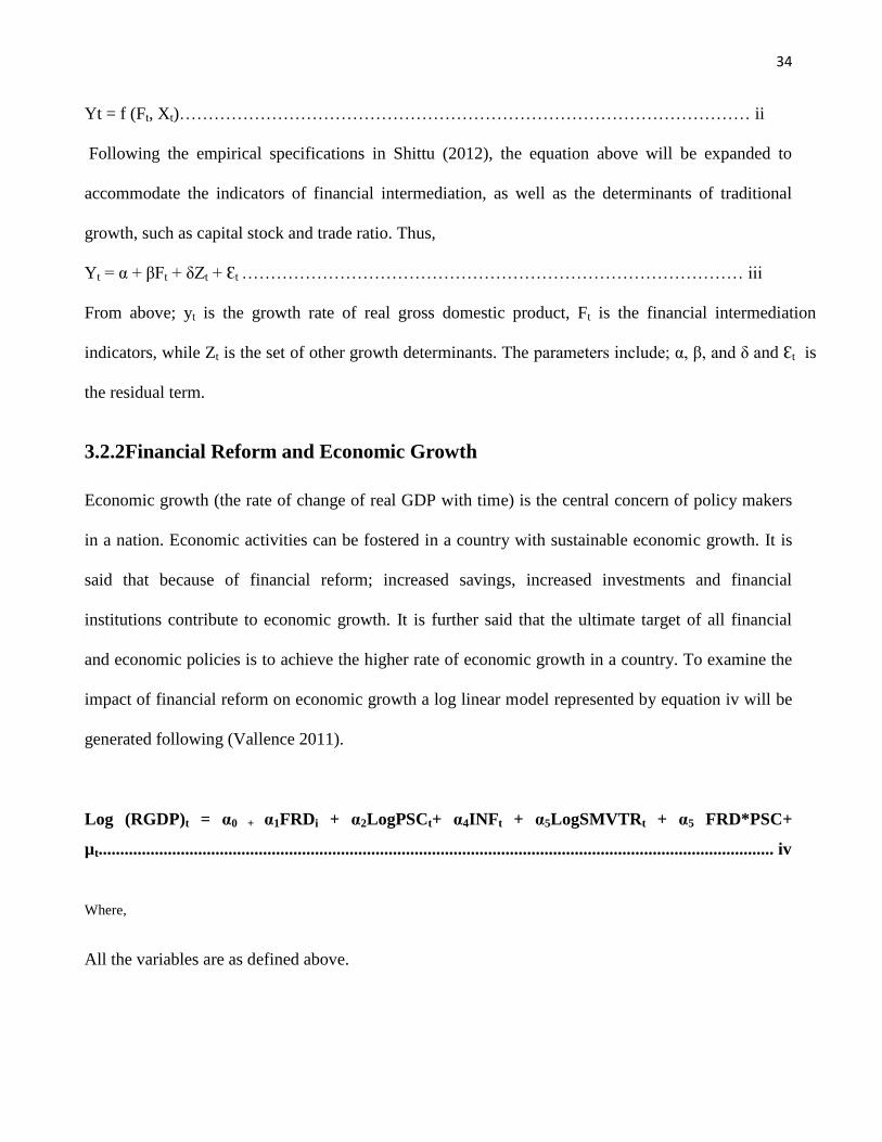
34
Yt = f (Ft, Xt)……………………………………………………………………………………… ii
Following the empirical specifications in Shittu (2012), the equation above will be expanded to
accommodate the indicators of financial intermediation, as well as the determinants of traditional
growth, such as capital stock and trade ratio. Thus,
Yt = α + βFt + δZt + Ɛt …………………………………………………………………………… iii
From above; yt is the growth rate of real gross domestic product, Ft is the financial intermediation
indicators, while Zt is the set of other growth determinants. The parameters include; α, β, and δ and Ɛt is
the residual term.
3.2.2Financial Reform and Economic Growth
Economic growth (the rate of change of real GDP with time) is the central concern of policy makers
in a nation. Economic activities can be fostered in a country with sustainable economic growth. It is
said that because of financial reform; increased savings, increased investments and financial
institutions contribute to economic growth. It is further said that the ultimate target of all financial
and economic policies is to achieve the higher rate of economic growth in a country. To examine the
impact of financial reform on economic growth a log linear model represented by equation iv will be
generated following (Vallence 2011).
Log (RGDP)t = α0 + α1FRDi + α2LogPSCt+ α4INFt + α5LogSMVTRt + α5 FRD*PSC+
µt............................................................................................................................................................ iv
Where,
All the variables are as defined above.
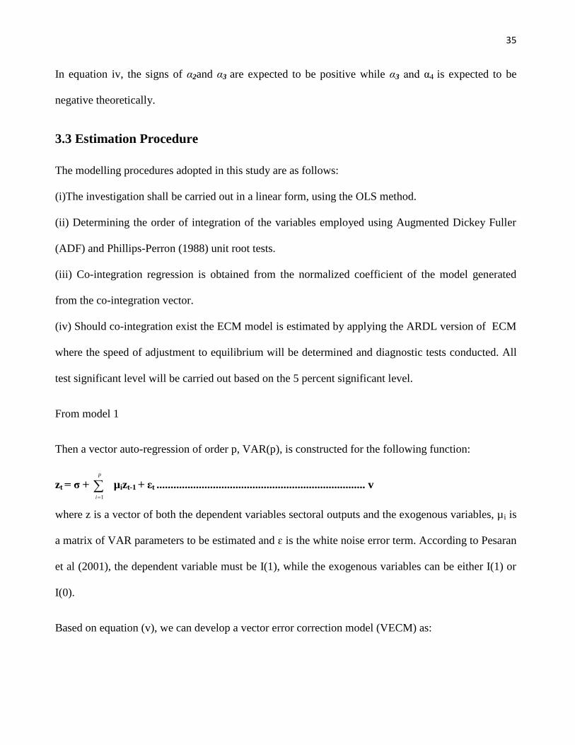
35
In equation iv, the signs of α2and α3 are expected to be positive while α3 and α4 is expected to be
negative theoretically.
3.3 Estimation Procedure
The modelling procedures adopted in this study are as follows:
(i)The investigation shall be carried out in a linear form, using the OLS method.
(ii) Determining the order of integration of the variables employed using Augmented Dickey Fuller
(ADF) and Phillips-Perron (1988) unit root tests.
(iii) Co-integration regression is obtained from the normalized coefficient of the model generated
from the co-integration vector.
(iv) Should co-integration exist the ECM model is estimated by applying the ARDL version of ECM
where the speed of adjustment to equilibrium will be determined and diagnostic tests conducted. All
test significant level will be carried out based on the 5 percent significant level.
From model 1
Then a vector auto-regression of order p, VAR(p), is constructed for the following function:
zt = σ +
p
i 1
µizt-1 + εt .......................................................................... v
where z is a vector of both the dependent variables sectoral outputs and the exogenous variables, µi is
a matrix of VAR parameters to be estimated and ɛ is the white noise error term. According to Pesaran
et al (2001), the dependent variable must be I(1), while the exogenous variables can be either I(1) or
I(0).
Based on equation (v), we can develop a vector error correction model (VECM) as:
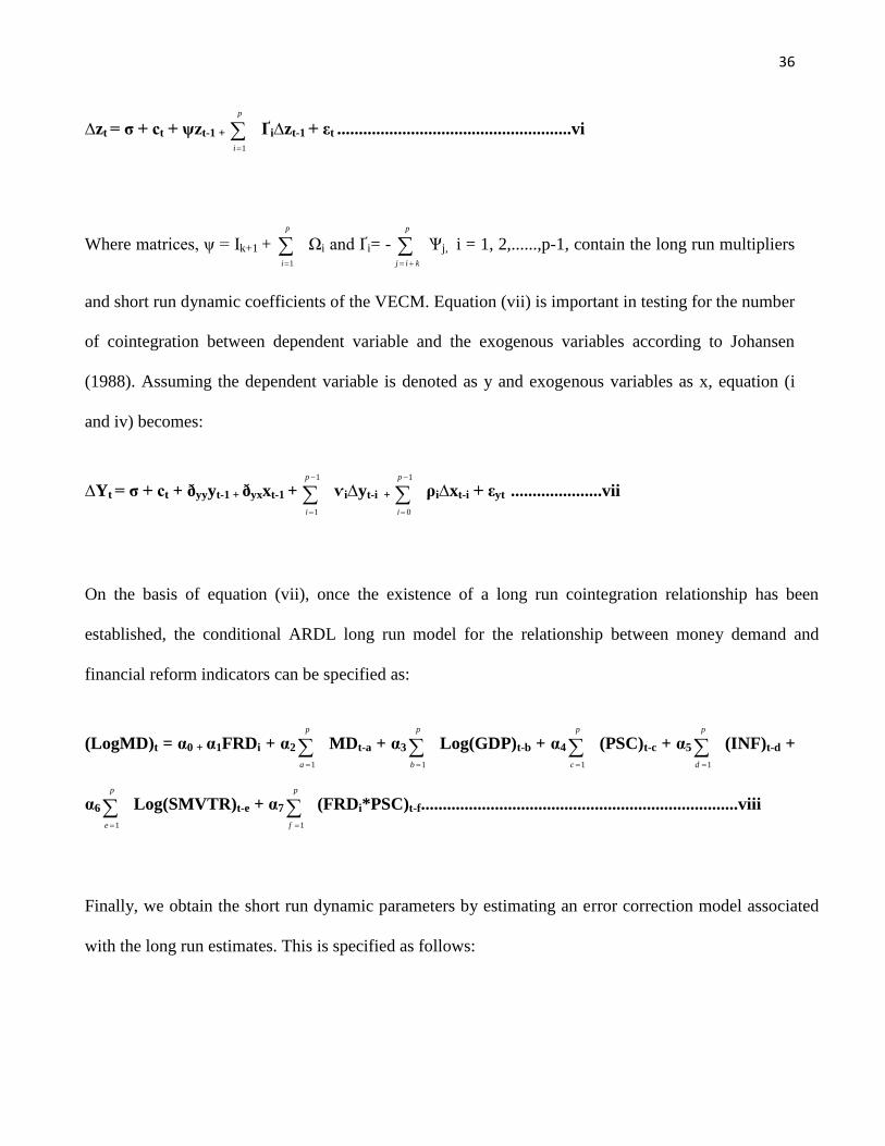
36
∆zt = σ + ct + ψzt-1 +
p
i 1
Ґi∆zt-1 + εt ......................................................vi
Where matrices, ψ = Ik+1 +
p
i 1
Ωi and Ґi= -
p
kij
Ѱj, i = 1, 2,......,p-1, contain the long run multipliers
and short run dynamic coefficients of the VECM. Equation (vii) is important in testing for the number
of cointegration between dependent variable and the exogenous variables according to Johansen
(1988). Assuming the dependent variable is denoted as y and exogenous variables as x, equation (i
and iv) becomes:
∆Yt = σ + ct + ðyyyt-1 + ðyxxt-1 +
1
1
p
i
ѵi∆yt-i +
1
0
p
i
ρi∆xt-i + εyt .....................vii
On the basis of equation (vii), once the existence of a long run cointegration relationship has been
established, the conditional ARDL long run model for the relationship between money demand and
financial reform indicators can be specified as:
(LogMD)t = α0 + α1FRDi + α2
p
a 1
MDt-a + α3
p
b 1
Log(GDP)t-b + α4
p
c 1
(PSC)t-c + α5
p
d 1
(INF)t-d +
α6
p
e 1
Log(SMVTR)t-e + α7
p
f 1
(FRDi*PSC)t-f.........................................................................viii
Finally, we obtain the short run dynamic parameters by estimating an error correction model associated
with the long run estimates. This is specified as follows:
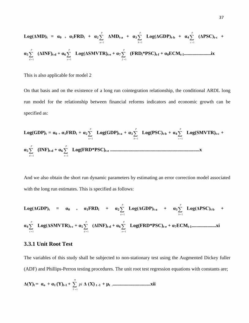
37
Log(ΔMD)t = α0 + α1FRDi + α2
p
a 1
ΔMDt-a + α3
p
b 1
Log(ΔGDP)t-b + α4
p
c 1
(ΔPSC)t-c +
α5
p
d 1
(ΔINF)t-d + α6
p
e 1
Log(ΔSMVTR)t-e + α7
p
f 1
(FRDi*PSC)t-f + α8ECMt-1......................ix
This is also applicable for model 2
On that basis and on the existence of a long run cointegration relationship, the conditional ARDL long
run model for the relationship between financial reforms indicators and economic growth can be
specified as:
Log(GDP)t = α0 + α1FRDi + α2
p
a 1
Log(GDP)t-a + α3
p
b 1
Log(PSC)t-b + α4
p
c 1
Log(SMVTR)t-c +
α5
p
d 1
(INF)t-d + α6
p
e 1
Log(FRD*PSC)t-e .........................................................................x
And we also obtain the short run dynamic parameters by estimating an error correction model associated
with the long run estimates. This is specified as follows:
Log(ΔGDP)t = α0 + α1FRDi + α2
p
a 1
Log(ΔGDP)t-a + α3
p
b 1
Log(ΔPSC)t-b +
α4
p
c 1
Log(ΔSMVTR)t-c + α5
p
d 1
(ΔINF)t-d + α6
p
e 1
Log(FRD*PSC)t-e + α7ECMt-1....................xi
3.3.1 Unit Root Test
The variables of this study shall be subjected to non-stationary test using the Augmented Dickey fuller
(ADF) and Phillips-Perron testing procedures. The unit root test regression equations with constants are;
Δ(Y)t = αo + α1 (Y)t-1 +
m
T
pi
1
Δ (X) t -1 + µt ................................xii
38
Where Δ is the difference operator
Ut and vt = random terms
t = linear trend
m = no of lagged differences.
3.4 Justification of the Model
This research work will employed Ordinary Least Square (OLS) estimation because of its reliable
qualities as the best unbiased estimator and because the equations were in recursive form. Since the focus
of the study is to establish the link between financial reforms, money demand and growth, based on the
aforementioned theoretical postulates and following the practices in most studies, an appropriate
technique is to adopt the autoregressive distributed Lag-error correction modeling (ARDL-ECM) and co-
integration approach popularized by pesaran et al (2001). The ARDL modelling approach is used
because it does not require pre-testing of the series to determine the order of integration when the
variables are of the mixed order of integration 1(0) and 1(1). Also the ARDL modelling incorporates
sufficient number of lags to capture the data generating process and is highly suitable when the sample
size is relatively small (Pesaran et al 2001).
3.5 Preliminary tests on variables of the study
Empirical tests would be conducted for normality, stationarity, multicolinearity and cointegration to
find out the nature of the variables before adopting them in various models for practical analysis.
39
3.5.1 Testing for normality
Normality is a condition in which the variables to be used in the model follow the standard normal
distribution.
The Jarque-Bera statistics will used to test the normality of the variable under different conditions
and under the hypotheses;
Ho: The series is normally distributed
H1: The series is not normally distributed
If the series are normally distributed, the histogram should be bell shaped and the Jarque-Bera
statistic insignificant. It thus follows that series will be normally distributed at 5% level of
significance if the probability of J-B statistic is greater than 0.05 and if consideration is made to 10%
level of significance, then the series are normally distributed if the probability of J-B statistics is
greater than 0.1.
3.5.2 Testing for stationarity
Unit root test being the preliminary step for econometric analysis of time series data, basically in the
cointegration tests, the test results will be achieved assuming the presence of unit root (non stationary
of the variable) in the null hypothesis (H0) and no unit root (stationary of the variable) in the
alternative hypothesis (H1). In this regard, decisions will be made based on the calculated statistic
and McKinnon‘s critical value in comparison with the critical values.
A variable will be considered non stationary if its calculated value is less than the Mackinnon‘s
critical value in critical values and we justify the existence of a unit root. On the other hand, a
variable will be considered stationary if its calculated value is higher than the critical value in
40
absolute terms and this confirmed the absence of unit root. These values will be generated using the
ADF test in E-views.
For the lag length of k; the tests had a maximum lag of 4 and down to the appropriate lag by
examining the Akaike Information criterion (AIC). The target will be to minimize residuals which is
indicated by the minimum AIC.
Using non-stationary variables to perform a regression generates spurious results and in most cases
leads to poor forecasts. Differencing the non-stationary variable(s) may make it stationary by
removing the trend due to growth rate (Volgen, 2005). With this in place non-stationarity will be
corrected by taking the first difference of the series. The target is to achieve the stationarity at the
minimum AIC.
3.5.3 Testing for serial correlation.
Serial correlation is usually a result of model mis-specification or genuine autocorrelation of the
model error term. In the presence of such a phenomenon, ordinary least squares are no longer BLUE
(Best Linear Unbiased Estimators). In such cases R-squared may be over-estimated. In case we have
lagged dependent variable to the right hand side, OLS estimators are biased and inconsistent. There
will be, thus every need to test for serial correlation in the residuals.
In this study the Durbin-Watson statistic will be used, to test for the first order autocorrelation. DW
statistic measures linear association, between adjacent residuals from a regression model. It will be
based on the hypotheses:
Ho: ρ=0, i.e. no serial correlation
H1: ρ=1 i.e. presence of serial correlation
The rule of thumb is that DW≈2, i.e. there is no serial correlation
DW< 2, implies a positive serial correlation and
41
DW > 2 implies presence of a negative serial correlation. However DW test becomes invalid if there
are lagged dependent variables to the right hand side of the regression and it is also dependant on the
distribution of the data matrix in question. This dependence can be handled by placing bounds on the
critical region. Being aware of the weaknesses of DW test, reliance will be made to the Correlogram
Q-statistics as a confirmatory test to DW test. This test Correlogram Q-statistic displays both the
autocorrelation and partial correlation functions of the residuals together with the Ljung-Box Q-
statistics for high order serial correlation. In presence of serial correlation, the autocorrelation and
partial correlations at all lags will be around zero and all Q-statistics will be significant.
3.6 Data and Sources
Annual secondary data sourced from the Central Bank of Nigeria statistical bulletins and World Bank
Development Indicators records covering the period 1970-2012 will be used in this study.
3.7 Econometric Software
E-views version 8.0 will be used for model estimation in this study.
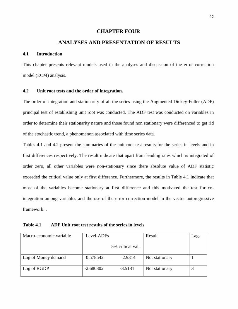
42
CHAPTER FOUR
ANALYSES AND PRESENTATION OF RESULTS
4.1 Introduction
This chapter presents relevant models used in the analyses and discussion of the error correction
model (ECM) analysis.
4.2 Unit root tests and the order of integration.
The order of integration and stationarity of all the series using the Augmented Dickey-Fuller (ADF)
principal test of establishing unit root was conducted. The ADF test was conducted on variables in
order to determine their stationarity nature and those found non stationary were differenced to get rid
of the stochastic trend, a phenomenon associated with time series data.
Tables 4.1 and 4.2 present the summaries of the unit root test results for the series in levels and in
first differences respectively. The result indicate that apart from lending rates which is integrated of
order zero, all other variables were non-stationary since there absolute value of ADF statistic
exceeded the critical value only at first difference. Furthermore, the results in Table 4.1 indicate that
most of the variables become stationary at first difference and this motivated the test for co-
integration among variables and the use of the error correction model in the vector autoregressive
framework. .
Table 4.1 ADF Unit root test results of the series in levels
Macro-economic variable Level-ADFs
5% critical val.
Result Lags
Log of Money demand -0.578542 -2.9314 Not stationary 1
Log of RGDP -2.680302 -3.5181 Not stationary 3
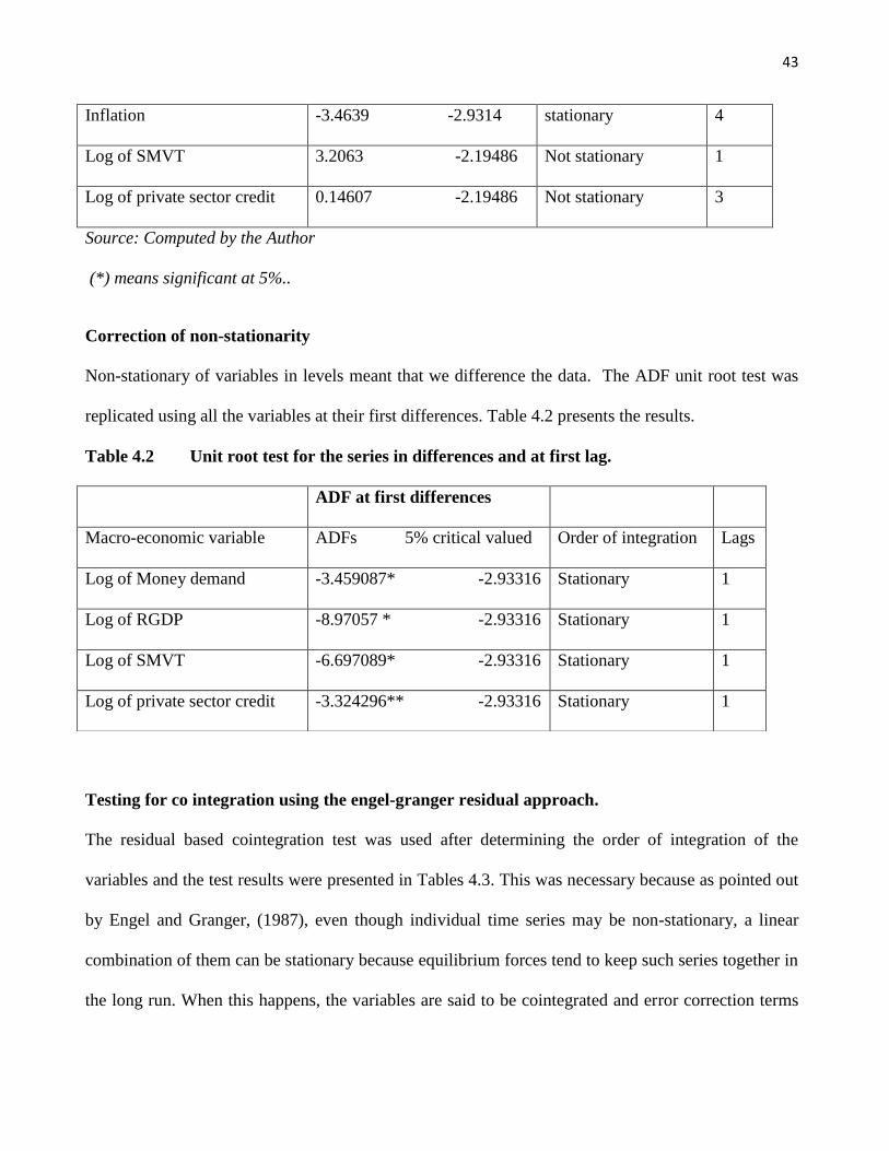
43
Inflation -3.4639 -2.9314 stationary 4
Log of SMVT 3.2063 -2.19486 Not stationary 1
Log of private sector credit 0.14607 -2.19486 Not stationary 3
Source: Computed by the Author
(*) means significant at 5%..
Correction of non-stationarity
Non-stationary of variables in levels meant that we difference the data. The ADF unit root test was
replicated using all the variables at their first differences. Table 4.2 presents the results.
Table 4.2 Unit root test for the series in differences and at first lag.
Testing for co integration using the engel-granger residual approach.
The residual based cointegration test was used after determining the order of integration of the
variables and the test results were presented in Tables 4.3. This was necessary because as pointed out
by Engel and Granger, (1987), even though individual time series may be non-stationary, a linear
combination of them can be stationary because equilibrium forces tend to keep such series together in
the long run. When this happens, the variables are said to be cointegrated and error correction terms
ADF at first differences
Macro-economic variable ADFs 5% critical valued Order of integration Lags
Log of Money demand -3.459087* -2.93316 Stationary 1
Log of RGDP -8.97057 * -2.93316 Stationary 1
Log of SMVT -6.697089* -2.93316 Stationary 1
Log of private sector credit -3.324296** -2.93316 Stationary 1
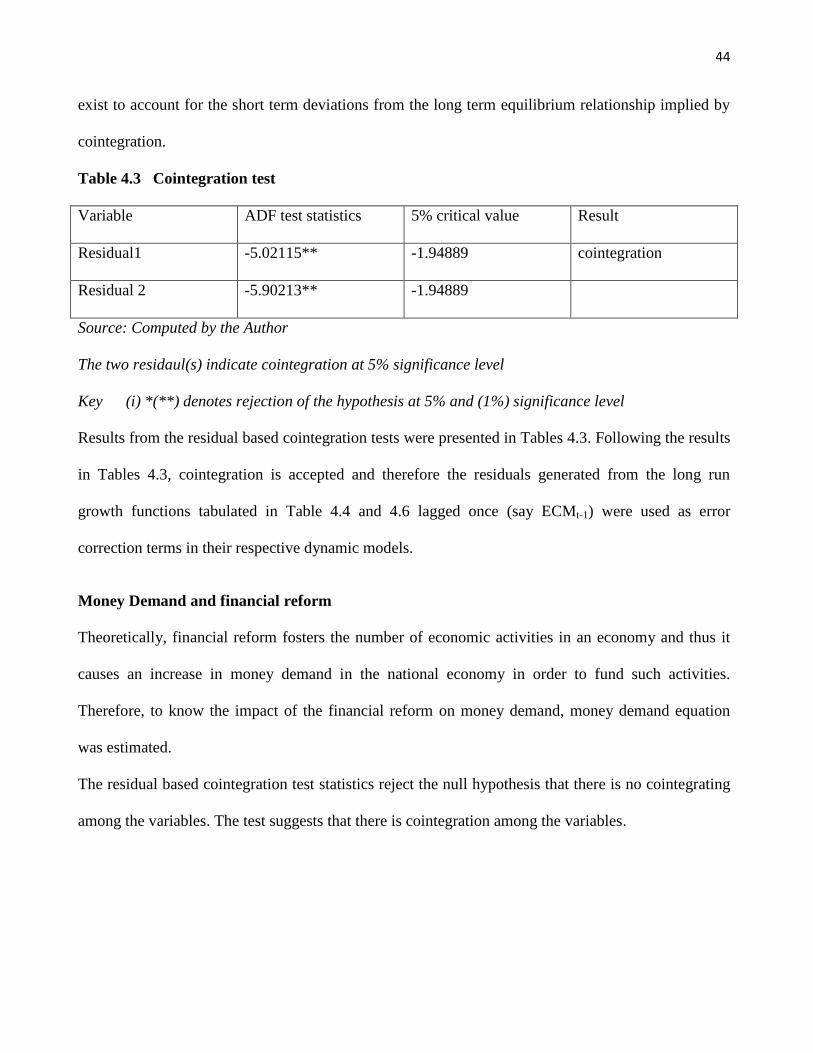
44
exist to account for the short term deviations from the long term equilibrium relationship implied by
cointegration.
Table 4.3 Cointegration test
Variable ADF test statistics 5% critical value Result
Residual1 -5.02115** -1.94889 cointegration
Residual 2 -5.90213** -1.94889
Source: Computed by the Author
The two residaul(s) indicate cointegration at 5% significance level
Key (i) *(**) denotes rejection of the hypothesis at 5% and (1%) significance level
Results from the residual based cointegration tests were presented in Tables 4.3. Following the results
in Tables 4.3, cointegration is accepted and therefore the residuals generated from the long run
growth functions tabulated in Table 4.4 and 4.6 lagged once (say ECMt-1) were used as error
correction terms in their respective dynamic models.
Money Demand and financial reform
Theoretically, financial reform fosters the number of economic activities in an economy and thus it
causes an increase in money demand in the national economy in order to fund such activities.
Therefore, to know the impact of the financial reform on money demand, money demand equation
was estimated.
The residual based cointegration test statistics reject the null hypothesis that there is no cointegrating
among the variables. The test suggests that there is cointegration among the variables.
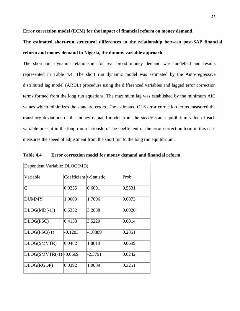
45
Error correction model (ECM) for the impact of financial reform on money demand.
The estimated short-run structural differences in the relationship between post-SAP financial
reform and money demand in Nigeria, the dummy variable approach.
The short run dynamic relationship for real broad money demand was modelled and results
represented in Table 4.4. The short run dynamic model was estimated by the Auto-regressive
distributed lag model (ARDL) procedure using the differenced variables and lagged error correction
terms formed from the long run equations. The maximum lag was established by the minimum AIC
values which minimizes the standard errors. The estimated OLS error correction terms measured the
transitory deviations of the money demand model from the steady state equilibrium value of each
variable present in the long run relationship. The coefficient of the error correction term in this case
measures the speed of adjustment from the short run to the long run equilibrium.
Table 4.4 Error correction model for money demand and financial reform
Dependent Variable: DLOG(MD)
Variable Coefficient t-Statistic Prob.
C 0.0235 0.6001 0.5531
DUMMY 1.0003 1.7696 0.0873
DLOG(MD(-1)) 0.6352 3.2888 0.0026
DLOG(PSC) 0.4153 3.5229 0.0014
DLOG(PSC(-1) -0.1283 -1.0889 0.2851
DLOG(SMVTR) 0.0482 1.8819 0.0699
DLOG(SMVTR(-1) -0.0669 -2.3791 0.0242
DLOG(RGDP) 0.0392 1.0009 0.3251
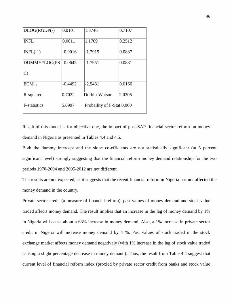
46
DLOG(RGDP(-) 0.0101 1.3746 0.7107
INFL 0.0011 1.1709 0.2512
INFL(-1) -0.0016 -1.7915 0.0837
DUMMY*LOG(PS
C)
-0.0645 -1.7951 0.0831
ECMt-1 -0.4492 -2.5431 0.0166
R-squared 0.7022 Durbin-Watson 2.0305
F-statistics 5.6997 Probaility of F-Stat.0.000
Result of this model is for objective one, the impact of post-SAP financial sector reform on money
demand in Nigeria as presented in Tables 4.4 and 4.5.
Both the dummy intercept and the slope co-efficients are not statistically significant (at 5 percent
significant level) strongly suggesting that the financial reform money demand relationship for the two
periods 1970-2004 and 2005-2012 are not different.
The results are not expected, as it suggests that the recent financial reform in Nigeria has not affected the
money demand in the country.
Private sector credit (a measure of financial reform), past values of money demand and stock value
traded affects money demand. The result implies that an increase in the lag of money demand by 1%
in Nigeria will cause about a 63% increase in money demand. Also, a 1% increase in private sector
credit in Nigeria will increase money demand by 41%. Past values of stock traded in the stock
exchange market affects money demand negatively (with 1% increase in the lag of stock value traded
causing a slight percentage decrease in money demand). Thus, the result from Table 4.4 suggest that
current level of financial reform index (proxied by private sector credit from banks and stock value
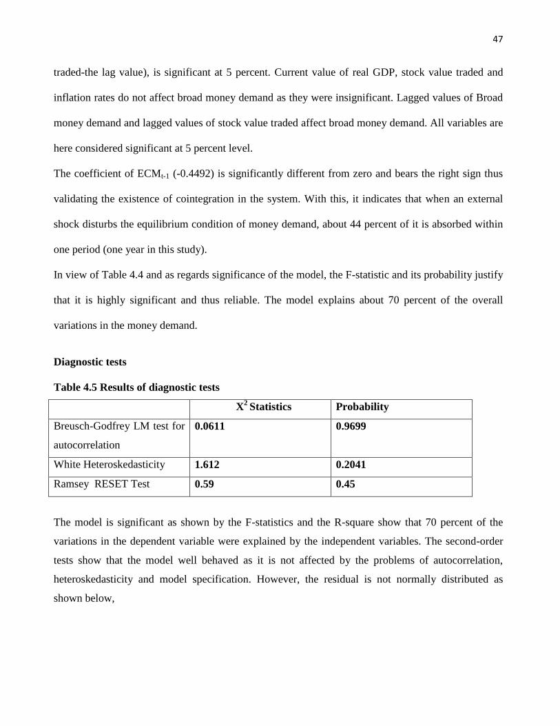
47
traded-the lag value), is significant at 5 percent. Current value of real GDP, stock value traded and
inflation rates do not affect broad money demand as they were insignificant. Lagged values of Broad
money demand and lagged values of stock value traded affect broad money demand. All variables are
here considered significant at 5 percent level.
The coefficient of ECMt-1 (-0.4492) is significantly different from zero and bears the right sign thus
validating the existence of cointegration in the system. With this, it indicates that when an external
shock disturbs the equilibrium condition of money demand, about 44 percent of it is absorbed within
one period (one year in this study).
In view of Table 4.4 and as regards significance of the model, the F-statistic and its probability justify
that it is highly significant and thus reliable. The model explains about 70 percent of the overall
variations in the money demand.
Diagnostic tests
Table 4.5 Results of diagnostic tests
X2
Statistics Probability
Breusch-Godfrey LM test for
autocorrelation
0.0611 0.9699
White Heteroskedasticity 1.612 0.2041
Ramsey RESET Test 0.59 0.45
The model is significant as shown by the F-statistics and the R-square show that 70 percent of the
variations in the dependent variable were explained by the independent variables. The second-order
tests show that the model well behaved as it is not affected by the problems of autocorrelation,
heteroskedasticity and model specification. However, the residual is not normally distributed as
shown below,
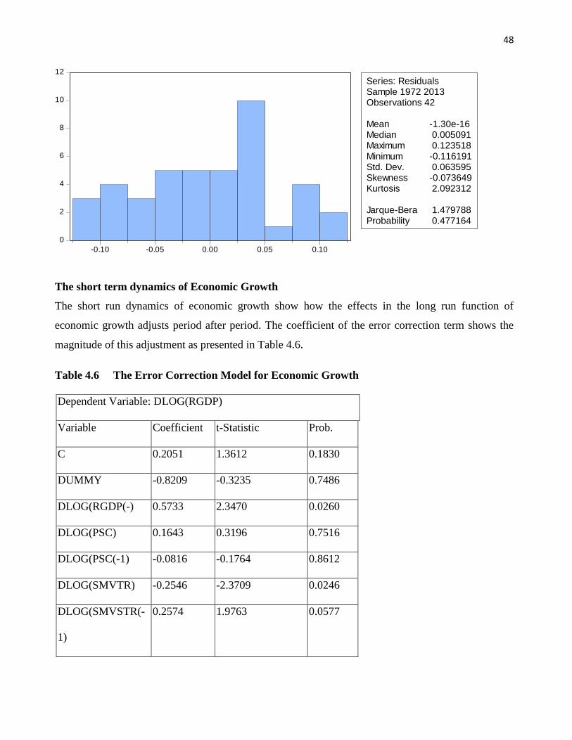
48
0
2
4
6
8
10
12
-0.10 -0.05 0.00 0.05 0.10
Series: ResidualsSample 1972 2013Observations 42
Mean -1.30e-16Median 0.005091Maximum 0.123518Minimum -0.116191Std. Dev. 0.063595Skewness -0.073649Kurtosis 2.092312
Jarque-Bera 1.479788Probability 0.477164
The short term dynamics of Economic Growth
The short run dynamics of economic growth show how the effects in the long run function of
economic growth adjusts period after period. The coefficient of the error correction term shows the
magnitude of this adjustment as presented in Table 4.6.
Table 4.6 The Error Correction Model for Economic Growth
Dependent Variable: DLOG(RGDP)
Variable Coefficient t-Statistic Prob.
C 0.2051 1.3612 0.1830
DUMMY -0.8209 -0.3235 0.7486
DLOG(RGDP(-) 0.5733 2.3470 0.0260
DLOG(PSC) 0.1643 0.3196 0.7516
DLOG(PSC(-1) -0.0816 -0.1764 0.8612
DLOG(SMVTR) -0.2546 -2.3709 0.0246
DLOG(SMVSTR(-
1)
0.2574 1.9763 0.0577
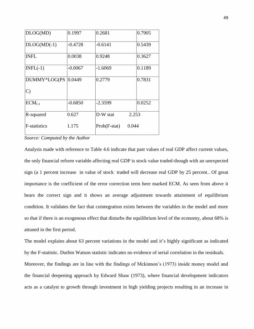
49
DLOG(MD) 0.1997 0.2681 0.7905
DLOG(MD(-1) -0.4728 -0.6141 0.5439
INFL 0.0038 0.9248 0.3627
INFL(-1) -0.0067 -1.6069 0.1189
DUMMY*LOG(PS
C)
0.0449 0.2779 0.7831
ECMt-1 -0.6850 -2.3599 0.0252
R-squared 0.627
F-statistics 1.175
D-W stat 2.253
Prob(F-stat) 0.044
Source: Computed by the Author
Analysis made with reference to Table 4.6 indicate that past values of real GDP affect current values,
the only financial reform variable affecting real GDP is stock value traded-though with an unexpected
sign (a 1 percent increase in value of stock traded will decrease real GDP by 25 percent.. Of great
importance is the coefficient of the error correction term here marked ECM. As seen from above it
bears the correct sign and it shows an average adjustment towards attainment of equilibrium
condition. It validates the fact that cointegration exists between the variables in the model and more
so that if there is an exogenous effect that disturbs the equilibrium level of the economy, about 68% is
attuned in the first period.
The model explains about 63 percent variations in the model and it‘s highly significant as indicated
by the F-statistic. Durbin Watson statistic indicates no evidence of serial correlation in the residuals.
Moreover, the findings are in line with the findings of Mckinnon‘s (1973) inside money model and
the financial deepening approach by Edward Shaw (1973), where financial development indicators
acts as a catalyst to growth through investment in high yielding projects resulting in an increase in
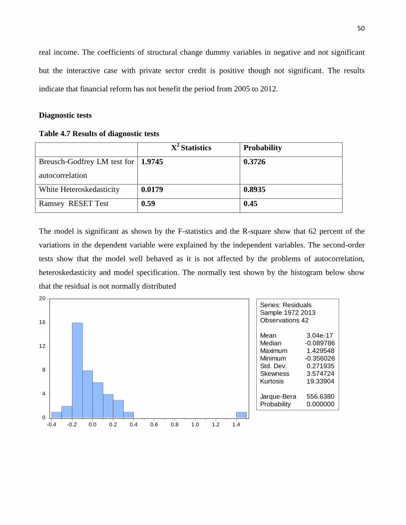
50
real income. The coefficients of structural change dummy variables in negative and not significant
but the interactive case with private sector credit is positive though not significant. The results
indicate that financial reform has not benefit the period from 2005 to 2012.
Diagnostic tests
Table 4.7 Results of diagnostic tests
X2
Statistics Probability
Breusch-Godfrey LM test for
autocorrelation
1.9745 0.3726
White Heteroskedasticity 0.0179 0.8935
Ramsey RESET Test 0.59 0.45
The model is significant as shown by the F-statistics and the R-square show that 62 percent of the
variations in the dependent variable were explained by the independent variables. The second-order
tests show that the model well behaved as it is not affected by the problems of autocorrelation,
heteroskedasticity and model specification. The normally test shown by the histogram below show
that the residual is not normally distributed
0
4
8
12
16
20
-0.4 -0.2 0.0 0.2 0.4 0.6 0.8 1.0 1.2 1.4
Series: ResidualsSample 1972 2013Observations 42
Mean 3.04e-17Median -0.089786Maximum 1.429548Minimum -0.356026Std. Dev. 0.271935Skewness 3.574724Kurtosis 19.33904
Jarque-Bera 556.6380Probability 0.000000
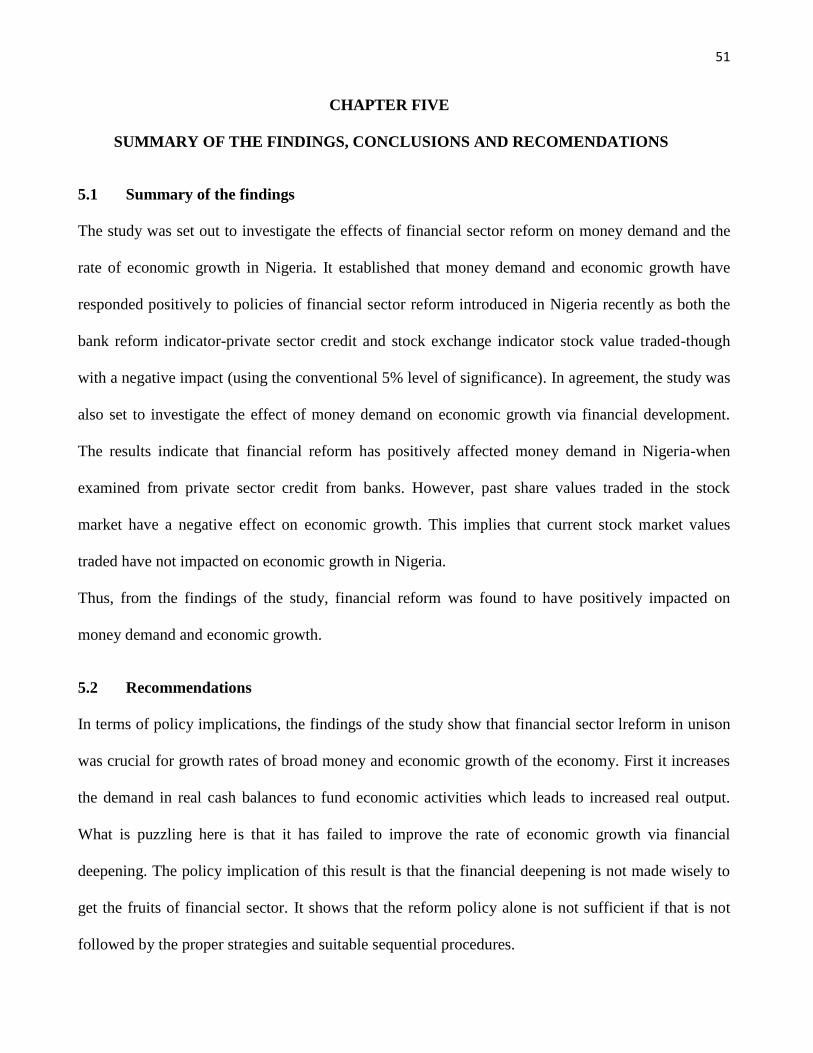
51
CHAPTER FIVE
SUMMARY OF THE FINDINGS, CONCLUSIONS AND RECOMENDATIONS
5.1 Summary of the findings
The study was set out to investigate the effects of financial sector reform on money demand and the
rate of economic growth in Nigeria. It established that money demand and economic growth have
responded positively to policies of financial sector reform introduced in Nigeria recently as both the
bank reform indicator-private sector credit and stock exchange indicator stock value traded-though
with a negative impact (using the conventional 5% level of significance). In agreement, the study was
also set to investigate the effect of money demand on economic growth via financial development.
The results indicate that financial reform has positively affected money demand in Nigeria-when
examined from private sector credit from banks. However, past share values traded in the stock
market have a negative effect on economic growth. This implies that current stock market values
traded have not impacted on economic growth in Nigeria.
Thus, from the findings of the study, financial reform was found to have positively impacted on
money demand and economic growth.
5.2 Recommendations
In terms of policy implications, the findings of the study show that financial sector lreform in unison
was crucial for growth rates of broad money and economic growth of the economy. First it increases
the demand in real cash balances to fund economic activities which leads to increased real output.
What is puzzling here is that it has failed to improve the rate of economic growth via financial
deepening. The policy implication of this result is that the financial deepening is not made wisely to
get the fruits of financial sector. It shows that the reform policy alone is not sufficient if that is not
followed by the proper strategies and suitable sequential procedures.
52
Therefore, policies that promote financial development and intermediation should be promoted.
Government can for instance improve intermediation by reducing taxation on the financial sector and
give incentives for its development. An integration of the fragmented financial markets is highly
desirable. The current experiment with financial reform and restructuring that are designed to
improve the efficiency of financial intermediaries will lead to economic growth only if inflation is
controlled and lending and deposit rates put under desirable seals. Depositors must be motivated to
deposit by increasing the deposit rates while investors must be motivated to use financial
intermediaries by lowering the lending rates. This is hoped to improve on the effect of financial
development to economic growth.
There is also every need to cut down the bureaucratic procedures in the process of financial reform
lending and depositing money which as a cost is accounted on the clients in favour of the financial
intermediaries. In other words bureaucracy among other factors makes financial intermediation costly
and are responsible for the narrow and costly sizes of financial assets availed by financial institutions
Moreover, financial sector reforms in particular suppose to induce structural changes, augment money
demand simultaneously with economic growth. But for these variables to exhibit rising contributions,
the government should continue with financial liberalization policy in particular. Emphasis should be
put on structural reforms such as promoting a competitive and viable domestic banking system, with
an adequate regulatory and supervisory framework. This should be complemented by macroeconomic
stability that is, fiscal deficits, rapidly depreciating exchange rate and high inflation should be put in
check. This calls for appropriate sequencing of the structural reforms. In implementing such reforms,
it is wiser to move gradually and to improve economic fundamentals first before complete
deregulation of any policy component.
53
5.3 Conclusions
Most studies in Nigeria have been taking components of financial reform individually as explanatory
variables. Other studies are found either to treat the partial financial reform of SAP as the full
liberalisation, or exclude the partial liberalisation period by taking only the full liberalisation date.
This is misleading, especially with the recent financial sector reforms. The trend of events calls for a
major and continued liberty of major variables of the economic system.
This study investigates the impact of financial reform as a result of financial sector reforms initiated
in 2005 on the demand for money and economic growth. Co-integration and auto-regressive
distributed lag model was applied to time series data from 1970 to 2013. The study found that
financial innovation has had some macroeconomic impact, which includes among others, the
reduction of the pressure on over-the-counter services to bank customers and improvement in the
operational efficiency in the banking system.
To assess the impact of innovation on the demand for money, we modelled our money demand
function to include two different proxies for financial innovation. We then proceeded to test whether
the macroeconomic variables entering the model were nonstationary.
Given that most of the series were non-stationary we conducted co-integration tests to determine
whether these variables were co-integrated. Following, an error correction model was formulated and
regression ran for the M1 and M2 monetary aggregates.
The results obtained have shown that all the macroeconomic variables affecting the demand for
money follow an integrated process. The series were found to be co-integrated. The error correction
equation gave results, some of, which were fully consistent with a priori restrictions The results show
a long-run influence of income, inflation, exchange rate and financial innovation on the demand for
M1 and income, inflation and innovation12 on the demand for M2. The error correction modelling on
54
the other hand indicated the absence of short-run currency substitution and inflation dynamics in the
demand for real M1 and the absence of short-run currency substitution in the demand for real M2.
The others with significant shortrun effects on the demand for M1 include income and financial
innovation whilst the demand for M2 has income, inflation and financial innovation exerting
significant short-run effects.
It is important to emphasize that the role of financial innovation was quantitatively important in the
demand for both narrow and broad money. Thus it is important for modelling it. In the long run we
observe that financial innovation has had a positive impact on the demand for both narrow and broad
money. In the short-run dynamics however, financial innovation had a negative impact on the
demand for broad money (M2) whereas its positive impact on the demand for narrow money
remained unchanged even in the short-run.
The demand for M1 and M2 was found to be very stable during the period under review, meaning
that the demand for real balances continues to remain stable despite the influx of new financial
products and process innovations by both banking and non-banking financial intermediaries resulting
from reforms in the financial sector. This may suggest that the growth in innovation has not been
rampart enough to distort the stability of the money demand function as postulated in the literature.
The results obtained for this study to a large extent supports both theoretical and empirical studies
that financial innovation does have macroeconomic impacts particularly affecting the macroeconomic
demand for money. This implies the relevant importance of the inclusion of financial innovation in
the estimation of the demand for money in Ghana.
55
5.4 Areas for further study
This study only considered the effect of financial sector reform on money demand and economic
growth. Due to time constraint and data limitations all the issues concerning money demand and
economic growth could not be analysed. The following areas are therefore recommended for further
research.
(i) Using the financial reform index to establish its effect on Government Expenditure.
(ii) Using the index, to study the impact of financial reform on other key macro-economic
variables like taxation, Imports and Exports.
(iii) To analyse the effect of financial sector reform using structural analysis
(iv) Since reform is not a one night stand policy, inclusion of other policy variables as may have
been deregulated at that time of the study is hoped to improve the results.
(v) To analyse the direction of causality between money demand and economic growth in the
banking and stock exchange reform era.
56
REFERENCES
Adebiyi (2006).On the stability of Demand for Money Function in Nigeria.Economic and Financial
Review, 42(3), 49-68.
Afangideh, U. J. (2010). Financial development and agricultural investment in Nigeria: historical
simulation approach. Journal of Economic and Monetary Integration, 9(1), 74-97.
Agu.C.C. (2008). Understanding the A.B.C of the Financial system; 42nd
inaugural lecture;Dec.4, 18-
19.
Aiyedogbon, J.O., S.E. Ibeh, M. Edafe, B.O. Ohwofasa (2013). Empirical analysis of money demand
function in Nigeria: 1986-2010. International Journal of Humanities and Social Science, 3(8),
Special Issue.
Akhand, A. H. and Sayera, Y. (2007).Interest Rates and the Demand for Money in Bangladesh.
Akinlo A.E. (2006). The stability of money demand in Nigeria: an autoregressive distributed lag
approach. Journal of Policy Modeling, 28(4), 445–452.
Allen, D.S. and Ndikumana, L (2000).Financial Intermediation and Economic Growth in Southern
Africa.Journal of African Economies, 9(2), 132-160.
Al-Samara, M. (2011).An Empirical Analysis of the Money Demand Function in Syria.Economic
Centre of Sorbonne,University of Paris-1 Panthéon-Sorbonne.
Anoruo, E. (2002) Stability of the Nigerian M2 Money Demand Function in the SAP Period,
Economics Bulletin, 14(3), 1-9.
Arestis, P. (2005). Financial Liberalisation and the relationship between Finance and Growth.
University of Cambridge, CEPP working paper 05/05.
Arrau, P., De Gregorio, J., Reinhart, C., Wickham, P. (1995). The demand for money in developing
countries: assessing the role of financial innovation. Journal of Development Economics 46
(2), 317-340.
Barnett,W.A. (1980).Economics Monetary Aggregates: An Application of Aggregation and Index
Number Theory. Journal of Econometrics 14, 11-48.
Bassey, Bassey Eyo, Bassong, Peter Kekung, Effiong ,Charles.(2012). The Effect of Monetary Policy
on Demand for Money in Nigeria. Interdisciplinary Journal of Contemporary Research in
Business, 4(7), 430.
Baumol, W.J. (1952). The Transactions Demand for Cash: An Inventory Theoretic Approach. The
Quarterly Journal of Economics, 66(4).
57
Bhatia, R.J. and Khatkhate, D.R. (1975). Financial Intermediation, Savings Mobilization, and
Entrepreneurial Development: The African Experience.IMF Staff Papers, 22(1), 132-158.
Bohamani – Oskooee, M. and M.P. Barry (2000b). Stability of the Demand for Money in an
Unstable Country: Russia. Journal of Keynesian Economics, 22(4), 619 – 629.
Boyd, J.H., Levine, R. and Smith, B.D. (2001).The Impact of Inflation on Financial
Sector Performance.Journal of Monetary Economics, 47, 221-248.
Busari, D.T. (2004). On the stability of Demand for Money Function in Nigeria Economic and
Financial review, 42(3) 49-68.
Busari, T.D. (2005). On the Stability of Money Demand Function in Nigeria. Financial and Economic
Review, CBN.
Bwire, T. (2007).Financial deepening, economic growth nexus in Uganda.
Caporale, G. M. and Gil-Alana, L. A. (2005).Fractional Cointegration and Aggregate Money Demand
Functions.The Manchester School, 73, 737-753.
CBN (2012). Central Bank of Nigeria Annual Report 2012: CBN publications {internet}. Available
from Google {Accessed 21st November, 2013}.
Chuku A.C. (2009). Measuring the Effect of Monetary Policy Inovations in Nigeria: A Structural
Vector Autoregrssive (SVAR), Approach.African Journal of Accounting, Economics, Finance
and Banking Research, 5(5).
Cuthbertson and Barlow, (1991). Money Demand Analysis: An outline in Money and Financial
Markets ed mark P. Taylor (Cambridge,Massachusetts: Basil Blackwell,Inc).
Cziraky D, Gillman M. (2006). Money demand in an EU accession country: a VECM study of
Croatia. Bulletin of Economic Research, 58(2), 73–159.
Dagher, J and Kovanen, A. (2011), On the Stability of Money Demand in Ghana: A bound Testing
Approach. International Monetary Fund Working Paper/11/273.
Darrat, A. F. and Al-Sowaidi, S. S. (2010). Information Technology, Financial Deepening and
Economic Growth: Some Evidence from a Fast Growing Emerging Economy. Journal
ofEconomics and International Finance, 2(2), 28-35.
Fisher, I. (1911). The Purchasing Power of Money. New York, Macmillian.
Fratzscher, M. and Bussière, M. (2004).Financial openness and growth: short-run gain, long run
pain?Working Paper Series 0348, European Central Bank.
Friedman, M. (1956). The Quantity Theory of Money-A Restatement in Studies in the Quantity of
Theory of Money, M. Friedman,ed, Chicago, IL.University of Chicago Press.
58
Friedman, M. (1959). The Demand for Money: Some Theoretical and Empirical Results. The Journal
of Political Economy, 67(4).
Gbadebo, O.O. and O.A. Okunrinboye (2009).Modelling the impact of financial innovation on money
demand in Nigeria. African Journal of Business Management, 3(2), 039-051.
Gbadebo, O.O. (2010). Does financial innovation affect the demand for money in Nigeria? Asian
Journal of business management studies, 1(1), 8-18.
Goldsmith, Raymond W. (1969). Financial Structure and Development, New Haven, Yale University
Press.
Gurley, J. and E. Shaw (1955).Financial Aspects of Economic Development.American Economic
Review, 45, 515-537.
Gurley, J.G. and S.S. Edward (1960).Money in aTheory of Finance. Washington, D.C. The Brookings
Institution.
Hoffman, D. L. and Robert H. R. (1991). Long –Run Income and Interest Elasticity of Money
Demand in United States. The Review of Economics and Statistics,73, 665-674.
Ighodaro, C. A. U and Ihaza, I.M. (2008).A Cointegration and Error Correction Approach to Broad
Money Demand in Nigeria.Journal of Research in National Development, 6(1).
Iyoboyi M. & Pedro, M.L. (2013). The Demand for Money in Nigeria: Evidence from Bounds
Testing Approach. Business and Economics Journal, 76.
Iyoha, M.A. (1976). The Demand for Money in Nigeria.Social and Economic StudiesInstitute of
Social and Economic Research, University of the West Indies, Jamaica, 25(4).
Jappelli, T. and M. Pagano (1994).Saving, Growth and Liquidity Constraints.Quarterly Journal of
Economics, 109, 83-109.
Johansen, S. (1988).Analysis of Cointegration Vector.Journal of Dynamic and Control, 12, 231 –
254.
Johansen, S. and Juselius, k. (1990). Maximum likelihood estimation andinference on cointegration
with applications to the demand for money.Oxford Bulletin of Economics and statistics,52(2),
169-210.
Keynes J.M. (1936). The Ex-Ante Theory of the Rate of Interest.The Economic Journal, 47.
King, R.G., and R. Levine. (1993). Finance, entrepreneurship and growth: Theory and evidence.
Journal of Monetary Economics, 32(3), 513-542.
59
Kumar, M.A. et al (2012). Analyzing soundness in Indian banking: A CAMEL Approach, Research
journal of Management Science, 1(3), 9-14.
Laidler, D. E. W. (1977). The demand for money: theories and evidence (2nd edition), New York,
Harper and Row.
Lucas, R. (1988a). On the Mechanics of Economic Development.Journal of Monetary Economics 22,
2-42.
Lucas, R. (1988b). Money demand in the United States: a quantitative review. Carnegie-Rochester
Conference Series on Public Policy, 29, 137–67.
McCallum, B. T. andGoodfriend, M.S. (1987). Demand for Money: Theoretical Studies in The New
Palgrave. John Eatwell, Murray Milgate, and Peter Newman (Eds.).W.W. Norton &
Company, Inc., London.
McKinnon, R.I. (1973). Money and Capital in Economic Development, Washington, DC, Brookings
Institution.
Miller, M.H., (1986). Financial Innovation: The last twenty years and the next. Journal of Financial
andQuantitative Analysis, 21(4), 459-471.
Neil, K.S. (2003). The Stability of M3 Money Demand and Monetary Targets; the Case of South
Africa.The Journal of Development Studies, 39(3), 151 – 180.
Nwaobi, G. (2002). A Vector Error Correction and Non-nested Modeling of Money Demand
Function in Nigeria.Economics Bulletin 3(4), 1 – 8.
Obamuyi T. M. (2009). An investigation of the relationship between interest rates and economic
growth in Nigeria, 1970 – 2006.Journal of Economics and International Finance, 1(4), 093-
098.
Odhiambo, N. M (2009).Interest Rate Liberalisation, Financial Deepening and Economic Growth in
South Africa.Ninth Annual IBER & TLC Conference Proceedings.
Ogun, O.D. (1986). A Note on Financial Deepening and Economic Growth: Evidence
from Africa. Nigerian Journal of Economic and Social Studies, 28(2), 275-283
Omotor, D.G. (2009). Money Demand and Foreign Exchange Risk for Nigeria: A Cointegration
Analysis using ARDL Test Processed.
Onaforowa, O.A. and O. Owoye (2007). Structural adjustments and the stability of the Nigerian
money demand function. International Business and Economics Research Journal, 3(8).
Oshikoya, T.W. (1992). Interest Rate Liberalization, Savings, Investment and Growth: the case of
Kenya, Savings and Development, 16(3), 305-320.
60
Pagano, M. (1993). Financial markets and growth: an overview. European Economic Review, 37,
613-622, WPS40, World Bank.
Patrick, H. (1966). Financial Development and Economic Growth in Underdeveloped Countries. In:
Economic Development and Cultural Change, 141(2), 174 – 189.
Perera, N. (1993).The Demand for Money and Monetary Policy: Evidence from Sri Lanka with
Cointegration Tests. Economics working paper, University of Wollongong, Australia.
Phillips, P. and Peron, P. (1988).Testing for a Unit Root in Time Series Regression, Biometrica, 75,
335-346.
Pesaran M.H., Shin Y and Smith R.J.(2001a). Bound testing approaches to the analysis of long run
relationships. Working Paper,University of Cambridge.
Pesaran, M. H., Yongcheol Shin, and Richard J.S. (2001b).Bounds Testing Approaches to the
Analysis of Level Relationships.Journal of Applied Econometrics, 16(3), 289-326.
Poole, W. (1988).Monetary policy lessons of recent inflation and disinflation‘, Journal ofEconomic
Perspectives, 2, 73–100.
Sanjay, K. (1998). Inflaction and Money Demand in Albania, Working Paper 98/101, IMF.
Sanya, O. (2013). Impact of Commodity Price Fluctuations on the Stability of Nigeria Money
Demand Function. International Journal of Arts and Commerce, 2(7).
Sanya, O. and A.A. Awe (2014). The Impact of financial liberalization on the stability of the Nigerian
money demand function. International Journal of Economics, Business and Finance, 2(1), 1-
18.
Shaw, E.S. (1973). Financial Deepening in Economic Development. New York, Oxford University
Press.
Stock, J. H. and Watson, M. W. (1993). A simple estimator of cointegrating vectors in higherorder
integrated systems, Econometrica, 61, 783–820.
Sriram, Subramanian S. (1999). Survey of Literature on Demand for Money, IMF Working Papers
99/64, International Monetary Fund.
Teriba, O. (1974). The Demand for Money in the Nigerian Economy: Some Methodological Issues
and Further Evidence. Nigerian Journal of Economic and Social Studies, 16(1), 153-164.
Tobin, J. (1956). The Interest-Elasticity of Transactions Demand for Cash.The Review of Economics
and Statistics, 38(3).
Tobin, James. (1958). Liquidity Preference as Behaviour Towards Risk. Review of Economic Studies
25(1), 65–86 (press +).
61
Vallence, N. (2011) The Effect of Financial Liberalization on Money Demand and Economic Growth,
Uganda‘s Experience, unpublished Manuscript.
Volgen, N. (2005). The Demand For Money and Monetary Policy: Evidence from Sri Lanka with
Cointegration Tests, Economics working paper, University of Wollongong, Australia.
Wesso, G.R. (2002). Broad Money Demand and Financial Liberalisation in South Africa. Occasional
Paper No. 18.
World Bank Group (2012). http://www.worldbank.org/. Retrieve on March 2012.
Yamden, P.B. (2011). The demand for money in Nigeria.European Journal of Business and
Management, 3(6), 63-85.
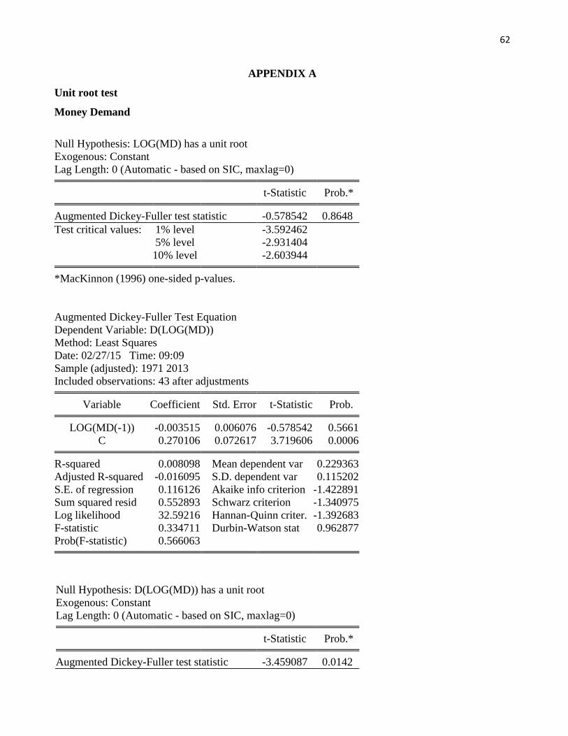
62
APPENDIX A
Unit root test
Money Demand
Null Hypothesis: LOG(MD) has a unit root
Exogenous: Constant
Lag Length: 0 (Automatic - based on SIC, maxlag=0)
t-Statistic Prob.*
Augmented Dickey-Fuller test statistic -0.578542 0.8648
Test critical values: 1% level -3.592462
5% level -2.931404
10% level -2.603944
*MacKinnon (1996) one-sided p-values.
Augmented Dickey-Fuller Test Equation
Dependent Variable: D(LOG(MD))
Method: Least Squares
Date: 02/27/15 Time: 09:09
Sample (adjusted): 1971 2013
Included observations: 43 after adjustments
Variable Coefficient Std. Error t-Statistic Prob.
LOG(MD(-1)) -0.003515 0.006076 -0.578542 0.5661
C 0.270106 0.072617 3.719606 0.0006
R-squared 0.008098 Mean dependent var 0.229363
Adjusted R-squared -0.016095 S.D. dependent var 0.115202
S.E. of regression 0.116126 Akaike info criterion -1.422891
Sum squared resid 0.552893 Schwarz criterion -1.340975
Log likelihood 32.59216 Hannan-Quinn criter. -1.392683
F-statistic 0.334711 Durbin-Watson stat 0.962877
Prob(F-statistic) 0.566063
Null Hypothesis: D(LOG(MD)) has a unit root
Exogenous: Constant
Lag Length: 0 (Automatic - based on SIC, maxlag=0)
t-Statistic Prob.*
Augmented Dickey-Fuller test statistic -3.459087 0.0142
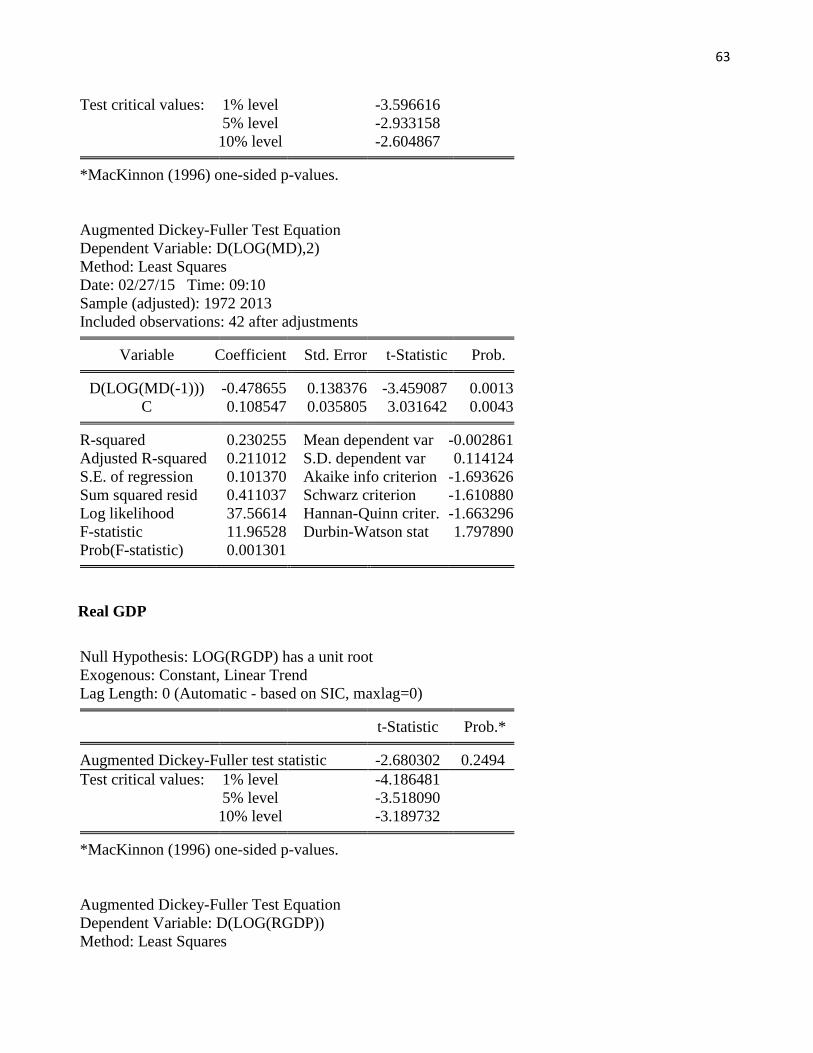
63
Test critical values: 1% level -3.596616
5% level -2.933158
10% level -2.604867
*MacKinnon (1996) one-sided p-values.
Augmented Dickey-Fuller Test Equation
Dependent Variable: D(LOG(MD),2)
Method: Least Squares
Date: 02/27/15 Time: 09:10
Sample (adjusted): 1972 2013
Included observations: 42 after adjustments
Variable Coefficient Std. Error t-Statistic Prob.
D(LOG(MD(-1))) -0.478655 0.138376 -3.459087 0.0013
C 0.108547 0.035805 3.031642 0.0043
R-squared 0.230255 Mean dependent var -0.002861
Adjusted R-squared 0.211012 S.D. dependent var 0.114124
S.E. of regression 0.101370 Akaike info criterion -1.693626
Sum squared resid 0.411037 Schwarz criterion -1.610880
Log likelihood 37.56614 Hannan-Quinn criter. -1.663296
F-statistic 11.96528 Durbin-Watson stat 1.797890
Prob(F-statistic) 0.001301
Real GDP
Null Hypothesis: LOG(RGDP) has a unit root
Exogenous: Constant, Linear Trend
Lag Length: 0 (Automatic - based on SIC, maxlag=0)
t-Statistic Prob.*
Augmented Dickey-Fuller test statistic -2.680302 0.2494
Test critical values: 1% level -4.186481
5% level -3.518090
10% level -3.189732
*MacKinnon (1996) one-sided p-values.
Augmented Dickey-Fuller Test Equation
Dependent Variable: D(LOG(RGDP))
Method: Least Squares
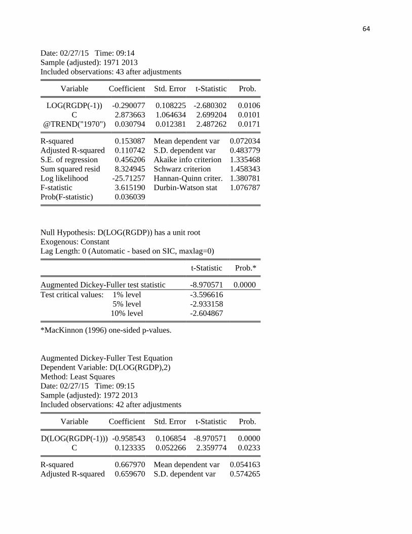
64
Date: 02/27/15 Time: 09:14
Sample (adjusted): 1971 2013
Included observations: 43 after adjustments
Variable Coefficient Std. Error t-Statistic Prob.
LOG(RGDP(-1)) -0.290077 0.108225 -2.680302 0.0106
C 2.873663 1.064634 2.699204 0.0101
@TREND("1970") 0.030794 0.012381 2.487262 0.0171
R-squared 0.153087 Mean dependent var 0.072034
Adjusted R-squared 0.110742 S.D. dependent var 0.483779
S.E. of regression 0.456206 Akaike info criterion 1.335468
Sum squared resid 8.324945 Schwarz criterion 1.458343
Log likelihood -25.71257 Hannan-Quinn criter. 1.380781
F-statistic 3.615190 Durbin-Watson stat 1.076787
Prob(F-statistic) 0.036039
Null Hypothesis: D(LOG(RGDP)) has a unit root
Exogenous: Constant
Lag Length: 0 (Automatic - based on SIC, maxlag=0)
t-Statistic Prob.*
Augmented Dickey-Fuller test statistic -8.970571 0.0000
Test critical values: 1% level -3.596616
5% level -2.933158
10% level -2.604867
*MacKinnon (1996) one-sided p-values.
Augmented Dickey-Fuller Test Equation
Dependent Variable: D(LOG(RGDP),2)
Method: Least Squares
Date: 02/27/15 Time: 09:15
Sample (adjusted): 1972 2013
Included observations: 42 after adjustments
Variable Coefficient Std. Error t-Statistic Prob.
D(LOG(RGDP(-1))) -0.958543 0.106854 -8.970571 0.0000
C 0.123335 0.052266 2.359774 0.0233
R-squared 0.667970 Mean dependent var 0.054163
Adjusted R-squared 0.659670 S.D. dependent var 0.574265
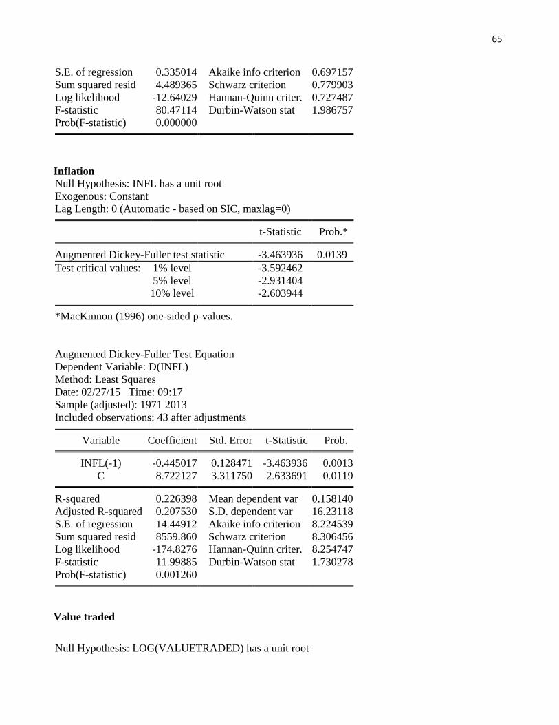
65
S.E. of regression 0.335014 Akaike info criterion 0.697157
Sum squared resid 4.489365 Schwarz criterion 0.779903
Log likelihood -12.64029 Hannan-Quinn criter. 0.727487
F-statistic 80.47114 Durbin-Watson stat 1.986757
Prob(F-statistic) 0.000000
Inflation
Null Hypothesis: INFL has a unit root
Exogenous: Constant
Lag Length: 0 (Automatic - based on SIC, maxlag=0)
t-Statistic Prob.*
Augmented Dickey-Fuller test statistic -3.463936 0.0139
Test critical values: 1% level -3.592462
5% level -2.931404
10% level -2.603944
*MacKinnon (1996) one-sided p-values.
Augmented Dickey-Fuller Test Equation
Dependent Variable: D(INFL)
Method: Least Squares
Date: 02/27/15 Time: 09:17
Sample (adjusted): 1971 2013
Included observations: 43 after adjustments
Variable Coefficient Std. Error t-Statistic Prob.
INFL(-1) -0.445017 0.128471 -3.463936 0.0013
C 8.722127 3.311750 2.633691 0.0119
R-squared 0.226398 Mean dependent var 0.158140
Adjusted R-squared 0.207530 S.D. dependent var 16.23118
S.E. of regression 14.44912 Akaike info criterion 8.224539
Sum squared resid 8559.860 Schwarz criterion 8.306456
Log likelihood -174.8276 Hannan-Quinn criter. 8.254747
F-statistic 11.99885 Durbin-Watson stat 1.730278
Prob(F-statistic) 0.001260
Value traded
Null Hypothesis: LOG(VALUETRADED) has a unit root
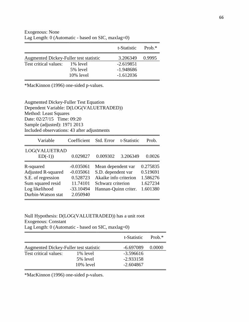
66
Exogenous: None
Lag Length: 0 (Automatic - based on SIC, maxlag=0)
t-Statistic Prob.*
Augmented Dickey-Fuller test statistic 3.206349 0.9995
Test critical values: 1% level -2.619851
5% level -1.948686
10% level -1.612036
*MacKinnon (1996) one-sided p-values.
Augmented Dickey-Fuller Test Equation
Dependent Variable: D(LOG(VALUETRADED))
Method: Least Squares
Date: 02/27/15 Time: 09:20
Sample (adjusted): 1971 2013
Included observations: 43 after adjustments
Variable Coefficient Std. Error t-Statistic Prob.
LOG(VALUETRAD
ED(-1)) 0.029827 0.009302 3.206349 0.0026
R-squared -0.035061 Mean dependent var 0.275835
Adjusted R-squared -0.035061 S.D. dependent var 0.519691
S.E. of regression 0.528723 Akaike info criterion 1.586276
Sum squared resid 11.74101 Schwarz criterion 1.627234
Log likelihood -33.10494 Hannan-Quinn criter. 1.601380
Durbin-Watson stat 2.050940
Null Hypothesis: D(LOG(VALUETRADED)) has a unit root
Exogenous: Constant
Lag Length: 0 (Automatic - based on SIC, maxlag=0)
t-Statistic Prob.*
Augmented Dickey-Fuller test statistic -6.697089 0.0000
Test critical values: 1% level -3.596616
5% level -2.933158
10% level -2.604867
*MacKinnon (1996) one-sided p-values.
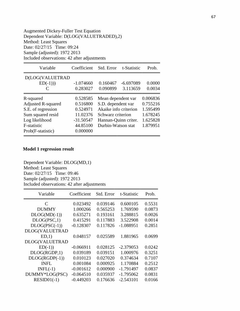
67
Augmented Dickey-Fuller Test Equation
Dependent Variable: D(LOG(VALUETRADED),2)
Method: Least Squares
Date: 02/27/15 Time: 09:24
Sample (adjusted): 1972 2013
Included observations: 42 after adjustments
Variable Coefficient Std. Error t-Statistic Prob.
D(LOG(VALUETRAD
ED(-1))) -1.074660 0.160467 -6.697089 0.0000
C 0.283027 0.090899 3.113659 0.0034
R-squared 0.528585 Mean dependent var 0.006836
Adjusted R-squared 0.516800 S.D. dependent var 0.755216
S.E. of regression 0.524971 Akaike info criterion 1.595499
Sum squared resid 11.02376 Schwarz criterion 1.678245
Log likelihood -31.50547 Hannan-Quinn criter. 1.625828
F-statistic 44.85100 Durbin-Watson stat 1.879951
Prob(F-statistic) 0.000000
Model 1 regression result
Dependent Variable: DLOG(MD,1)
Method: Least Squares
Date: 02/27/15 Time: 09:46
Sample (adjusted): 1972 2013
Included observations: 42 after adjustments
Variable Coefficient Std. Error t-Statistic Prob.
C 0.023492 0.039146 0.600105 0.5531
DUMMY 1.000266 0.565253 1.769590 0.0873
DLOG(MD(-1)) 0.635271 0.193161 3.288815 0.0026
DLOG(PSC,1) 0.415291 0.117883 3.522908 0.0014
DLOG(PSC(-1)) -0.128307 0.117826 -1.088951 0.2851
DLOG(VALUETRAD
ED,1) 0.048157 0.025589 1.881965 0.0699
DLOG(VALUETRAD
ED(-1)) -0.066911 0.028125 -2.379053 0.0242
DLOG(RGDP,1) 0.039189 0.039151 1.000976 0.3251
DLOG(RGDP(-1)) 0.010123 0.027020 0.374634 0.7107
INFL 0.001084 0.000925 1.170884 0.2512
INFL(-1) -0.001612 0.000900 -1.791497 0.0837
DUMMY*LOG(PSC) -0.064510 0.035937 -1.795062 0.0831
RESID01(-1) -0.449203 0.176636 -2.543101 0.0166
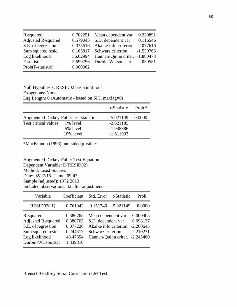
68
R-squared 0.702251 Mean dependent var 0.229891
Adjusted R-squared 0.579045 S.D. dependent var 0.116546
S.E. of regression 0.075616 Akaike info criterion -2.077616
Sum squared resid 0.165817 Schwarz criterion -1.539766
Log likelihood 56.62994 Hannan-Quinn criter. -1.880473
F-statistic 5.699796 Durbin-Watson stat 2.030581
Prob(F-statistic) 0.000062
Null Hypothesis: RESID02 has a unit root
Exogenous: None
Lag Length: 0 (Automatic - based on SIC, maxlag=0)
t-Statistic Prob.*
Augmented Dickey-Fuller test statistic -5.021149 0.0000
Test critical values: 1% level -2.621185
5% level -1.948886
10% level -1.611932
*MacKinnon (1996) one-sided p-values.
Augmented Dickey-Fuller Test Equation
Dependent Variable: D(RESID02)
Method: Least Squares
Date: 02/27/15 Time: 09:47
Sample (adjusted): 1972 2013
Included observations: 42 after adjustments
Variable Coefficient Std. Error t-Statistic Prob.
RESID02(-1) -0.761942 0.151746 -5.021149 0.0000
R-squared 0.380765 Mean dependent var -0.000405
Adjusted R-squared 0.380765 S.D. dependent var 0.098137
S.E. of regression 0.077226 Akaike info criterion -2.260645
Sum squared resid 0.244517 Schwarz criterion -2.219271
Log likelihood 48.47354 Hannan-Quinn criter. -2.245480
Durbin-Watson stat 1.839810
Breusch-Godfrey Serial Correlation LM Test:
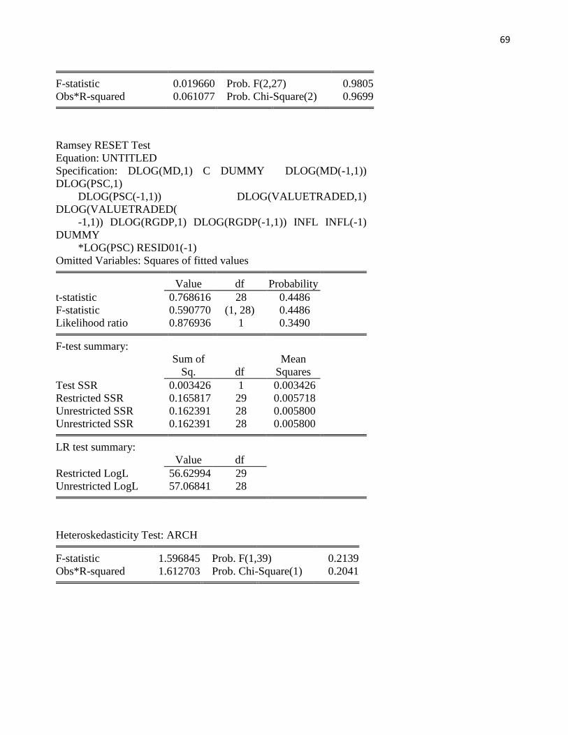
69
F-statistic 0.019660 Prob. F(2,27) 0.9805
Obs*R-squared 0.061077 Prob. Chi-Square(2) 0.9699
Ramsey RESET Test
Equation: UNTITLED
Specification: DLOG(MD,1) C DUMMY DLOG(MD(-1,1))
DLOG(PSC,1)
DLOG(PSC(-1,1)) DLOG(VALUETRADED,1)
DLOG(VALUETRADED(
-1,1)) DLOG(RGDP,1) DLOG(RGDP(-1,1)) INFL INFL(-1)
DUMMY
*LOG(PSC) RESID01(-1)
Omitted Variables: Squares of fitted values
Value df Probability
t-statistic 0.768616 28 0.4486
F-statistic 0.590770 (1, 28) 0.4486
Likelihood ratio 0.876936 1 0.3490
F-test summary:
Sum of
Sq. df
Mean
Squares
Test SSR 0.003426 1 0.003426
Restricted SSR 0.165817 29 0.005718
Unrestricted SSR 0.162391 28 0.005800
Unrestricted SSR 0.162391 28 0.005800
LR test summary:
Value df
Restricted LogL 56.62994 29
Unrestricted LogL 57.06841 28
Heteroskedasticity Test: ARCH
F-statistic 1.596845 Prob. F(1,39) 0.2139
Obs*R-squared 1.612703 Prob. Chi-Square(1) 0.2041
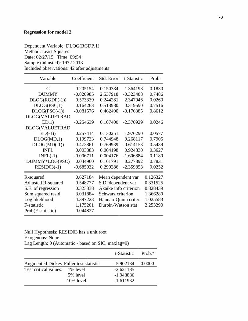
70
Regression for model 2
Dependent Variable: DLOG(RGDP,1)
Method: Least Squares
Date: 02/27/15 Time: 09:54
Sample (adjusted): 1972 2013
Included observations: 42 after adjustments
Variable Coefficient Std. Error t-Statistic Prob.
C 0.205154 0.150384 1.364198 0.1830
DUMMY -0.820985 2.537918 -0.323488 0.7486
DLOG(RGDP(-1)) 0.573339 0.244281 2.347046 0.0260
DLOG(PSC,1) 0.164263 0.513980 0.319590 0.7516
DLOG(PSC(-1)) -0.081576 0.462490 -0.176385 0.8612
DLOG(VALUETRAD
ED,1) -0.254639 0.107400 -2.370929 0.0246
DLOG(VALUETRAD
ED(-1)) 0.257414 0.130251 1.976290 0.0577
DLOG(MD,1) 0.199733 0.744948 0.268117 0.7905
DLOG(MD(-1)) -0.472861 0.769939 -0.614153 0.5439
INFL 0.003883 0.004198 0.924830 0.3627
INFL(-1) -0.006711 0.004176 -1.606884 0.1189
DUMMY*LOG(PSC) 0.044960 0.161791 0.277892 0.7831
RESID03(-1) -0.685032 0.290286 -2.359853 0.0252
R-squared 0.627184 Mean dependent var 0.126327
Adjusted R-squared 0.548777 S.D. dependent var 0.331525
S.E. of regression 0.323338 Akaike info criterion 0.828439
Sum squared resid 3.031884 Schwarz criterion 1.366289
Log likelihood -4.397223 Hannan-Quinn criter. 1.025583
F-statistic 1.175201 Durbin-Watson stat 2.253290
Prob(F-statistic) 0.044827
Null Hypothesis: RESID03 has a unit root
Exogenous: None
Lag Length: 0 (Automatic - based on SIC, maxlag=9)
t-Statistic Prob.*
Augmented Dickey-Fuller test statistic -5.902134 0.0000
Test critical values: 1% level -2.621185
5% level -1.948886
10% level -1.611932
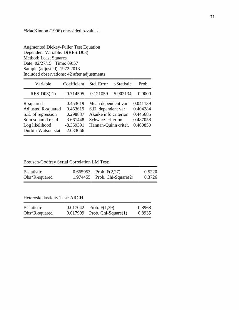
71
*MacKinnon (1996) one-sided p-values.
Augmented Dickey-Fuller Test Equation
Dependent Variable: D(RESID03)
Method: Least Squares
Date: 02/27/15 Time: 09:57
Sample (adjusted): 1972 2013
Included observations: 42 after adjustments
Variable Coefficient Std. Error t-Statistic Prob.
RESID03(-1) -0.714505 0.121059 -5.902134 0.0000
R-squared 0.453619 Mean dependent var 0.041139
Adjusted R-squared 0.453619 S.D. dependent var 0.404284
S.E. of regression 0.298837 Akaike info criterion 0.445685
Sum squared resid 3.661448 Schwarz criterion 0.487058
Log likelihood -8.359391 Hannan-Quinn criter. 0.460850
Durbin-Watson stat 2.033066
Breusch-Godfrey Serial Correlation LM Test:
F-statistic 0.665953 Prob. F(2,27) 0.5220
Obs*R-squared 1.974455 Prob. Chi-Square(2) 0.3726
Heteroskedasticity Test: ARCH
F-statistic 0.017042 Prob. F(1,39) 0.8968
Obs*R-squared 0.017909 Prob. Chi-Square(1) 0.8935
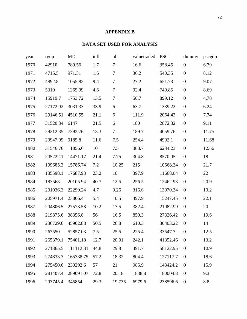
72
APPENDIX B
DATA SET USED FOR ANALYSIS
year rgdp MD infl plr valuetraded PSC dummy pscgdp
1970 42910 789.56 1.7 7 16.6 358.45 0 6.79
1971 4715.5 971.31 1.6 7 36.2 540.35 0 8.12
1972 4892.8 1055.82 9.4 7 27.2 651.73 0 9.07
1973 5310 1265.99 4.6 7 92.4 749.85 0 8.69
1974 15919.7 1753.72 13.5 7 50.7 899.12 0 4.78
1975 27172.02 3031.33 33.9 6 63.7 1339.22 0 6.24
1976 29146.51 4510.55 21.1 6 111.9 2064.43 0 7.74
1977 31520.34 6147 21.5 6 180 2872.32 0 9.11
1978 29212.35 7392.76 13.3 7 189.7 4059.76 0 11.75
1979 29947.99 9185.8 11.6 7.5 254.4 4902.1 0 11.68
1980 31546.76 11856.6 10 7.5 388.7 6234.23 0 12.56
1981 205222.1 14471.17 21.4 7.75 304.8 8570.05 0 18
1982 199685.3 15786.74 7.2 10.25 215 10668.34 0 21.7
1983 185598.1 17687.93 23.2 10 397.9 11668.04 0 22
1984 183563 20105.94 40.7 12.5 256.5 12462.93 0 20.9
1985 201036.3 22299.24 4.7 9.25 316.6 13070.34 0 19.2
1986 205971.4 23806.4 5.4 10.5 497.9 15247.45 0 22.1
1987 204806.5 27573.58 10.2 17.5 382.4 21082.99 0 20
1988 219875.6 38356.8 56 16.5 850.3 27326.42 0 19.6
1989 236729.6 45902.88 50.5 26.8 610.3 30403.22 0 14
1990 267550 52857.03 7.5 25.5 225.4 33547.7 0 12.5
1991 265379.1 75401.18 12.7 20.01 242.1 41352.46 0 13.2
1992 271365.5 111112.31 44.8 29.8 491.7 58122.95 0 10.9
1993 274833.3 165338.75 57.2 18.32 804.4 127117.7 0 18.6
1994 275450.6 230292.6 57 21 985.9 143424.2 0 15.9
1995 281407.4 289091.07 72.8 20.18 1838.8 180004.8 0 9.3
1996 293745.4 345854 29.3 19.735 6979.6 238596.6 0 8.8
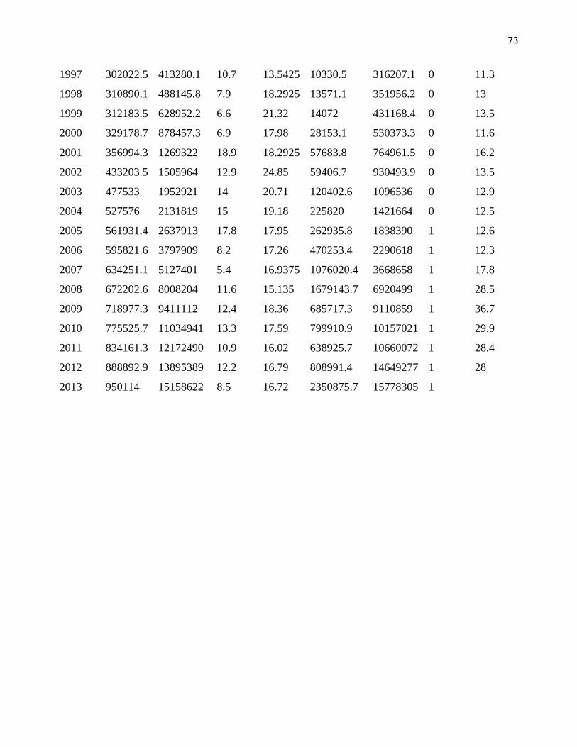
73
1997 302022.5 413280.1 10.7 13.5425 10330.5 316207.1 0 11.3
1998 310890.1 488145.8 7.9 18.2925 13571.1 351956.2 0 13
1999 312183.5 628952.2 6.6 21.32 14072 431168.4 0 13.5
2000 329178.7 878457.3 6.9 17.98 28153.1 530373.3 0 11.6
2001 356994.3 1269322 18.9 18.2925 57683.8 764961.5 0 16.2
2002 433203.5 1505964 12.9 24.85 59406.7 930493.9 0 13.5
2003 477533 1952921 14 20.71 120402.6 1096536 0 12.9
2004 527576 2131819 15 19.18 225820 1421664 0 12.5
2005 561931.4 2637913 17.8 17.95 262935.8 1838390 1 12.6
2006 595821.6 3797909 8.2 17.26 470253.4 2290618 1 12.3
2007 634251.1 5127401 5.4 16.9375 1076020.4 3668658 1 17.8
2008 672202.6 8008204 11.6 15.135 1679143.7 6920499 1 28.5
2009 718977.3 9411112 12.4 18.36 685717.3 9110859 1 36.7
2010 775525.7 11034941 13.3 17.59 799910.9 10157021 1 29.9
2011 834161.3 12172490 10.9 16.02 638925.7 10660072 1 28.4
2012 888892.9 13895389 12.2 16.79 808991.4 14649277 1 28
2013 950114 15158622 8.5 16.72 2350875.7 15778305 1