The impact of climate and CO2 change on potential winter

wheat yields in the Netherlands from 1981 to 2010

Abram het Lam

MSc thesis Plant Production Systems

February 2014

The impact of climate and CO2 on potential winter wheat yields in the

Netherlands from 1981 to 2010

Abram het Lam

MSc thesis Plant Production Systems

PPS80436

February 2014

Supervisors:

prof.dr.ir. M.K. van Ittersum

ing. H.C.A. Rijk

Examiners:

dr.ir.ing. A.G.T. Schut

Foreword This research is carried out in the context of my MSc program ‘Plant Sciences’ at the faculty of Plant

Production Systems of Wageningen University.

The research is based on modelling work. Although modelling might seem quite impersonal work, I

had a quite intense relationship with the LINTUL model. If it worked I was very excited about its

output, although sometimes it turned out there was something wrong beneath the shiny top layer of

the results. There were, however, also many times when it did not do what I wanted and I did not

know what was wrong. In the end we found a compromise, LINTUL gave me outputs and I accepted

not everything was perfect. In the mean time we have shared a wedding, a move and an internship.

Since the research is at its end, I would like to thank the people around me who supported me during

this adventure. Firstly, I would like to thank my supervisors Martin van Ittersum and Bert Rijk for

their time, support and guidance which kept me sharp and close to reality. I would like to thank Joost

Wolf as well, for his fast and clear support regarding the LINTUL model. Of course I am also very

grateful to my wife, Sanne, for her support and patience during the process. Furthermore, I much

appreciated the quiet and atmospheric working place, provided by PPS. Finally, I would like to thank

my examiners for the time and interest they invest in my work.

Kind regards,

Abram

Contents Foreword ................................................................................................................................................. 3

Contents .................................................................................................................................................. 4

Summary ................................................................................................................................................. 6

1 Introduction ...................................................................................................................................... 8

2 Materials and Methods ................................................................................................................... 12

2.1 Regression analyses ............................................................................................................... 12

2.1.1 Yield ................................................................................................................................... 12

2.1.2 Area ................................................................................................................................... 12

2.1.3 Climate ............................................................................................................................... 12

2.1.4 Correlation between yield and climate ............................................................................. 14

2.2 Modelling ............................................................................................................................... 15

2.2.1 The LINTUL model ............................................................................................................. 15

2.2.2 Calibration of the model.................................................................................................... 20

2.2.3 Validation........................................................................................................................... 23

2.2.4 Model for current varieties ............................................................................................... 23

2.2.5 Model limitations .............................................................................................................. 23

2.2.6 Simulation .......................................................................................................................... 24

3 Results ............................................................................................................................................. 26

3.1 Area and yield analyses ......................................................................................................... 26

3.1.1 Area ................................................................................................................................... 26

3.1.2 Yields .................................................................................................................................. 26

3.2 Weather and CO2 trends ....................................................................................................... 28

3.2.1 CO2 ..................................................................................................................................... 28

3.2.2 Weather ............................................................................................................................. 28

3.3 Correlation between winter wheat yields and weather factors and CO2 ............................. 30

3.3.1 Correlations between factors ............................................................................................ 30

3.3.2 Models with combined factors .......................................................................................... 30

3.4 Calibration ............................................................................................................................. 33

3.4.1 Development ..................................................................................................................... 33

3.4.2 Growth ............................................................................................................................... 35

3.5 Simulations ............................................................................................................................ 38

3.5.1 Influence of temperature change...................................................................................... 38

3.5.2 Influence of radiation change ............................................................................................ 38

3.5.3 Influence of CO2 change..................................................................................................... 42

3.5.4 Influence of actual weather .............................................................................................. 42

4 Discussion ........................................................................................................................................ 44

4.1 Yield ....................................................................................................................................... 44

4.2 Area ....................................................................................................................................... 45

4.3 Climate effects ....................................................................................................................... 46

4.3.1 Changes in climate ............................................................................................................. 46

4.3.2 Effects of changes in climate ............................................................................................. 47

4.3.3 Modelling ........................................................................................................................... 48

4.3.4 CO2 effect ........................................................................................................................... 51

4.3.5 Combined effect ................................................................................................................ 52

4.4 Drivers of yield trends ........................................................................................................... 52

4.4.1 Extreme events .................................................................................................................. 53

4.4.2 Ozone ................................................................................................................................. 54

4.4.3 UV-B ................................................................................................................................... 55

4.4.4 Management ..................................................................................................................... 55

5 Conclusions & Recommendations ................................................................................................... 57

5.1 Main findings ......................................................................................................................... 57

5.2 Recommendations................................................................................................................. 57

6 References ....................................................................................................................................... 59

7 Appendices ...................................................................................................................................... 64

Appendix I Results .............................................................................................................................. 65

Appendix II .......................................................................................................................................... 88

Appendix III ......................................................................................................................................... 89

6

Summary There are indications that winter wheat (Triticum aestivum L.) yields in North-western Europe are

stagnating since the 1990’s and that yield gaps are increasing. This will affect regional food

production and farm income. In the Netherlands genetic potential yields of winter wheat are still

linearly increasing since the 1980’s, however farm yields are not keeping up with the increase in

potential yields of variety trials. Reasons for the increasing yield gap might be changes in

environmental factors, including climate, or management. This research is aimed at unravelling the

influence of climate and CO2 on winter wheat yields from 1981 to 2010, using crop modelling.

Trends in yields and areas of winter wheat in the Netherlands were analysed using Genstat 14. Daily

weather data on average temperature, precipitation, incoming global radiation and reference

evapotranspiration and CO2 were analysed for trends. Furthermore, regression analyses were carried

out on the relation between climatic factors and winter wheat yields from 1981 to 2010. Potential

yields of winter wheat from 1981 to 2010 were simulated with the LINTUL1 model based on

temperature, radiation and CO2, separate and combined, for normal (10 October) and late sown (25

November) winter wheat based on current ‘varieties’ and varieties of the early 1980’s. Changes in

potential yields were analysed, based on separate climate factors as well as all climate factors

together.

There were no changes in winter wheat area. A linear increase in winter wheat yields of 66.3 kg ha-1

year-1 was found for the period of 1981 to 2010 and quadratic increases were found for periods

starting earlier than 1978 to 2010. CO2 concentrations in the air increased from 340 to 390 ppm from

1981 to 2010. For all stations analysed, average temperature during the growing season, from April

to July and from June to July increased linearly with 1.5, 1.83 and 0.725 oC in 30 years, respectively.

Incoming global radiation over the growing season and from April to July, increased linearly with ±

250 MJ m-2 in 30 years. Reference and actual evapotranspiration also increased linearly, with ± 50

mm over 30 years. Cumulative rainfall and precipitation deficit from April or June to July did not

show significant trends due to large annual variability. Winter wheat yields were negatively

correlated with average temperature over the growing season and rainfall from April to July. Positive

correlations with yields were found with precipitation deficits from April and June to July. Simulation

results show that temperature had no significant effect on potential winter wheat yields. Radiation

and CO2 both had a positive effect on wheat yields, with average increases of 10% and 20%

respectively. The effect of CO2 was non-linear, with diminishing increase with higher CO2 towards the

end of the analysed period. In this research, these climate factors together lead to an overall increase

of 31% in potential winter wheat yields, with the same non-linearity as found for CO2. The harvest

index of winter wheat declined from 0.51 to 0.47 on average, due to sink limitation of the grain.

The increase in potential yields due to changed weather together with genetic yields improvements

are not fully reflected in farm yields, indicating that there must be other (negative) influences. Many

factors could be responsible for this negative impact, including changes in extreme weather events,

UV-B radiation and management related issues. Management could have changed due to changing

regulations and other socioeconomic influences such as cereal prices. Changes in soil compaction,

fertilization, timing of management and extensification might also result in reduced yields. Further

research should aim at exploring these influences in more detail.

7

8

1 Introduction

‘How to feed the world?’ is one of the main questions in agronomic science these days. Due to fast

population growth, 9 billion people are expected to live on this planet in the year 2050 (FAO, 2002;

Godfray et al., 2010; FAO, 2009). Because of increasing wealth of people in developing countries,

dietary demands of the world population will change to more meat based meals (Godfray et al.,

2010; Spiertz and Ewert, 2009). Besides this, the meat that is consumed is shifting from ruminants,

which are fed with grassland products, to non-ruminants, which are fed with arable crop products

(Koning et al., 2008). These changes in human diets will amplify the increase in crop production

demand from arable land (Godfray et al., 2010; Spiertz and Ewert, 2009; Jaggard et al., 2010). Taking

all effects into account, 50 to 100% more food will be needed halfway this century (Godfray et al.,

2010; Jaggard et al., 2010; FAO, 2009). Increasing interest in the growing of biofuel crops as an

alternative energy source to fossil fuels, growing costs of fossil fuel supply and a growing energy

demand from developing countries, put even more pressure on agricultural production (Godfray et

al., 2010; Gregory and George, 2011; Spiertz and Ewert, 2009; Tweeten and Thompson, 2008).

In addition to a growing demand for production, the agricultural sector faces other challenges. Due

to climate change more and more extreme weather events occur all around the world (Gardner,

2010; Krugman, 2011; Peters, 2011; Romm, 2011; Spiertz and Ewert, 2009; Tweeten and Thompson,

2008). During the second half of the first decade of this century, global food production has been

significantly affected by droughts in Australia (Spiertz and Ewert, 2009; Tweeten and Thompson,

2008), Russia, China and Brazil and flooding in Australia, Brazil, and Pakistan (Gardner, 2010;

Krugman, 2011; Peters, 2011; Romm, 2011).

Although only about half of the 4.4 billion hectare of land suitable for agriculture on earth is currently

under arable cultivation (Part et al., 2011; Fischer et al., 2011), expansion of this cultivated area is not

a desirable strategy to increase crop food and feed production. Firstly, because the currently

cultivated land is the most productive land that is available (Fischer et al., 2011). So, increasing the

total crop production by cultivating extra land will take more and more effort and inputs. Secondly,

most of the well suited land for arable production is currently under forest, grassland or woodland,

which are inhabiting a vast spectrum of biological life (Fischer et al., 2011). According to Dobrovolski

et al. (2011) and Prins et al. (2011), agricultural expansion is the main cause of biodiversity loss,

mainly due to habitat loss. Finally, because of expansion of cities, the growth of other land use

activities like recreation and losses of high quality agricultural land due to degradation, options for

expansion of food and feed production area are limited even more (Godfray et al., 2010; Tweeten

and Thompson, 2008). While, Gregory & George (2011) estimate that only 20% of the total increase

in food production will come from expanding the area of crop production, Mandemaker et al. (2011)

warn that more expansion will occur, if global yields are not improved. Therefore increasing the

productivity of the current limited agricultural area is crucial to meet the growing demand for

agricultural products without biodiversity loss (Godfray et al., 2010; Jaggard et al., 2010; Spiertz and

Ewert, 2009).

Tweeten & Tompson (2008), report that cereals make up half of global human diets and two-third if

animal feed is included. Therefore cereal yield improvement is essential for increasing food

production overall (Fischer and Edmeades, 2010). In the second half of the twentieth century, indeed

a steady growth in average yields for the main cereal food crops was found (Fischer and Edmeades,

9

2010; Calderini and Slafer, 1998). This growth was fuelled by improving genetic potential of cereal

crops via breeding, as well as increasing use of inputs, like fertilizers, irrigation and crop protection

agents (Calderini and Slafer, 1998; Gervois et al., 2008). Recently however, several researches point

out that this growth is stagnating for some of the major cereal crops in several countries around the

world (Brisson et al., 2010; Calderini and Slafer, 1998). Calderini & Slafer (1998) report that there was

no yield improvement for wheat (Triticum aestivum L.) in Japan, USA, Canada, Tunisia, France and

the UK and even a decline in former USSR and in Spain in the period of 1985 to 1997. In agreement

with this, Slafer & Peltonen-Sainio (2001), Peltonen-Sainio (2009), Brisson et al. (2010) and Finger

(2010) show that growth in wheat yields in a large part of Europe stagnates since the mid-nineties of

the previous century.

Since the stagnation in wheat yield increments in Europe became clear, it has been suggested that

potential yields cannot be improved much more since a ceiling in genetic potential of the crop is

reached or approached via breeding (Jaggard et al., 2010; Calderini and Slafer, 1998). The idea

behind this is, that the biggest gains in yield come from an increased harvest index and the optimum

harvest index has almost been reached for most crops (Jaggard et al., 2010; Brisson et al., 2010;

Fischer and Edmeades, 2010; Peltonen-Sainio et al., 2009). Nevertheless, there are still a lot of other

traits that can be improved, for instance, light use efficiency or phenology (Jaggard et al., 2010;

Fischer and Edmeades, 2010; Spiertz and Ewert, 2009; Godfray et al., 2010; Peltonen-Sainio et al.,

2009). Trends in genetic potential of crops also show that in most cases there is still a linear genetic

progress in potential yields (Peltonen-Sainio et al., 2009; Brisson et al., 2010; Fischer and Edmeades,

2010). For winter wheat in the Netherlands, Rijk et al. (2013) found an average linear genetic yield

increase of 0.09 Mg ha-1 year-1 on marine clay. This is in accordance with results from Finland

(Peltonen-Sainio et al., 2009), France (Brisson et al., 2010) and the UK (Fischer and Edmeades, 2010),

although for Finland the magnitude of increase was much smaller i.e. 17 to 46 kg ha-1 year-1. So,

despite some suggestions, it is clear that the increase in genetic potential of wheat in the

Netherlands is not reaching a ceiling at this moment.

In practice, crop yields are determined by the interaction between three main factors. Namely, the

genotype of the crop (G), the environmental conditions in which the crop grows (E) and the

agricultural management that is imposed on the crop (M) (Messina et al., 2009; Loomis and Connor,

1992; Cooper and Hammer, 1996). Although management or agronomy is actually affecting the

environment of the crop, it is useful to separate E and M (Cooper and Hammer, 1996). (E) is then

considered the part of the environment that cannot be adapted easily, while (M) is the part that can

be adapted. Wheat yields are thus changing by changes in one or more of the factors in the GxExM

interaction.

In order to minimize the yield gap it is important to understand the aspects that determine current

yield levels. Van Ittersum & Rabbinge (1997), divide these aspects into three main categories. Firstly,

growth defining factors, which determine the potential yield if resources are optimally supplied and

there are no growth reducing pests, diseases or weeds. These factors include: incoming solar

radiation; temperature; CO2 levels; and genetic features of the crop variety. Secondly, growth

limiting factors including: available water and nutrients, which determine water and nutrient limited

crop yields. Thirdly, growth reducing factors, i.e. pests, diseases and weeds which reduce crop yields

if they are active, these result in actual yields on farms. Yield levels can be improved by making

adaptations to any factor in one of the three categories (Van Ittersum and Rabbinge, 1997). To close

10

the gap between actual yields and nutrient and water limited yields, pest and weed management,

seeding time, crop rotation and soil management must be improved. The gap between nutrient and

water limited and potential yields can be reduced by optimizing resource supply. Finally, also

potential yields can be improved, by breeding crop varieties with a higher yield potential under the

given biophysical conditions.

If the yield gap between potential and actual yields is increasing and genetic potential yield (G) of

winter wheat is not increasing slower than actual yield, it means that E or M are limiting or reducing

yield increase on-farm. Due to global warming, important environmental factors are changing and

predicted to change even more. Temperature, incoming solar radiation, CO2 concentrations in the air

and rainfall are the most important factors that change (Jaggard et al., 2010; Olesen and Bindi, 2002;

Brisson et al., 2010). It could thus be, that climate change reduces wheat yields, directly by altering

growth and development of the crop or indirectly by changing the effect of pests and diseases or

management (Godfray et al., 2010; Jaggard et al., 2010; Spiertz and Ewert, 2009; Prins et al., 2011;

Peltonen-Sainio et al., 2009; Olesen and Bindi, 2002; Gervois et al., 2008). Besides this, changes in

crop management (M) by farmers might be a reason for stagnating yields (Brisson et al., 2010; Van

Ittersum and Rabbinge, 1997; Peltonen-Sainio et al., 2009; Gervois et al., 2008; Hanse, 2011).

According to Brisson et al. (2010), the stagnation in Netherlands started after 1993. This trend was

not found by Rijk et al. (2013), however the latter found a decrease in realization of potential yields

gains at farm level, meaning an increasing yield gap. This increasing yield gap at farm level is not only

harmful for regional food supply, but can also be negative for farmer income.

To be able to steer future research and other efforts to reduce the yield gap of winter wheat, it is

important to clarify what the exact causes for the widening yield gap are in the Netherlands.

Therefore the effect of climate change on average winter wheat yields in the Netherlands from 1981

until now has been investigated. To this end data on average national winter wheat yields has been

analysed and the effect of climate change on wheat yields evaluated, using a crop growth model.

Since the cultivated area with winter wheat in the Netherlands is the largest of all grain crops, this is

focused on winter wheat only.

Research questions

The main question addressed in this research is: What is the effect of climate change on winter wheat

yields in the Netherlands from 1981 until 2010? This main question has been addressed via two sub-

questions. Firstly the trends in national and regional winter wheat yields in the Netherlands from

1981 until 2010 have been investigated. Secondly the effect of climatic conditions on national an

regional wheat yields in the Netherlands from 1981 until 2010 has been explored in three steps:

Is there a significant trend in CO2 concentration in the air, daily incoming solar radiation and

daily average temperatures during the growing season and in the total amount of rainfall in

the period from April to July, over the period of 1981 - 2010?

Is there a significant correlation between winter wheat yields and CO2 concentration in the

air, total incoming solar radiation and daily average temperatures during the growing

11

season and in the total rainfall deficit in the period from April till July, over the period of

1981 - 2010?

Are simulated winter wheat yields with measured climate data showing significant trends in

wheat yields over the period of 1981 - 2010?

12

2 Materials and Methods

2.1 Regression analyses

2.1.1 Yield

Data of national yields from 1970 to 2010 and regional winter wheat yields from 1981 to 2010 was

retrieved from the “Dutch Agricultural Economics Institute Foundation” (LEI) and “Statistics

Netherlands” (CBS) (CBS and LEI; LEI and CBS). The moisture content of the grain was 16%. Regional

yields were based on Dutch agricultural regions as classified by (CBS) (Fig. 3.1). The classification of

the agricultural regions was changed by the CBS between the years 1990 and 1991 (Fig. 3.1). Yield

records for similar areas from before and after the reclassification were merged if it was plausible

that the change did not affect yield trends. This plausibility was evaluated based on the overlap of

regions, differences in dominant soils types between old and new regions and the continuity of yield

trends before and after the switch. The following regions were used for the yield trend analyses:

‘Oostelijk veehouderijgebied’, ‘Centraal veehouderijgebied’, ‘Zuidelijk veehouderijgebied’,

‘Rivierengebied’, ‘IJsselmeerpolders’, ‘Zuidwestelijk akkerbouwgebied’ and ‘Zuid-Limburg’.

Trends in the national and regional yields were evaluated with linear, quadratic, exponential and

broken stick trend models, to select the best fitting model. Linear and quadratic models were

compared based on the F probability (P < 0.05) of change between the models with the linear

regression test, where a quadratic model was only used if significantly better. In addition to that, all

four models were compared on the basis of the adjusted R2. The statistical software program Genstat

14th edition (Payne et al., 2011) was used.

2.1.2 Area

The national and regional acreage of winter wheat in the Netherlands from 1980 to 2010 was

collected from the LEI (CBS) (CBS and LEI; LEI and CBS). As with yield data the areas were fit to linear

and quadratic models to investigate historical changes which could lead to changes in average yields.

Area data was available for all regions in the Netherlands. Therefore the regions ‘Hollands/Utrechts

weidegebied’,’ Waterland & Droogmakerijen’, ‘Bouwhoek & Hogeland’, ‘Veenkoloniën & Oldtambt’,

‘Westelijk Holland’ and ‘Zuid-West Brabant’ were also included in the regression analyses.

2.1.3 Climate

Daily values of incoming radiation, minimum and maximum temperatures, and amounts of rainfall

during the growing season (October – July) and monthly Makkink reference evapotranspiration from

April to July in the period from 1980 up to and including 2010 were downloaded from the Royal

Netherlands Meteorological Institute (KNMI) (KNMI, 2012) for all meteorological stations in the

Netherlands. For only four stations, ’De Bilt’, ‘Eelde’, ‘Vlissingen’ and ‘Maastricht’, the time series

from 1981 until 2010 were complete for all climate indicators. To get a better spatial coverage of the

country, data from station ‘Twenthe’ was added. For this station data on global radiation and

reference evapotranspiration before 1988 was missing. Monthly atmospheric CO2 concentrations

were collected from the ESRL Global Monitoring Division of the National Oceanic & Atmospheric

Administration in the USA (ESRL, 2012).

13

Figure 3.1 Classification of Agricultural regions in the Netherlands until (A) and after (B) 1990 according to CBS.

A B

14

To analyse the trends in the different climate factors, they were aggregated into a suitable temporal

format. Since crop growth model LINTUL, which will be used, is not designed for inserting monthly

CO2 values and trends in CO2 over different years not within years are assumed to be important, the

average CO2 concentration over the whole year was calculated from monthly values. Daily average

temperatures were calculated by dividing the sum of the minimum and maximum temperature per

day by two. To see the effect of average temperature on plant development as a whole, these values

were averaged over the growing season, mid-October to mid-July. In addition to this the average

temperatures from mid-June to mid-July and from mid-April to mid-July were computed to explore

the effect on heat stress during grain filling. Incoming solar radiation was accumulated for the entire

growing season. Monthly rainfall and Makkink reference evapotranspiration were accumulated for

the period of the season where water shortage can be limiting plant growth (mid-April – mid-July).

The actual evapotranspiration of wheat was estimated by combining reference evapotranspiration

with the wheat crop factors provided by KNMI (Hooghart, 1988). With the actual evapotranspiration

and rainfall data the precipitation deficit was calculated on a monthly basis.

2.1.4 Correlation between yield and climate

In order to find out which climate factors were important for simulating winter wheat yields in the

Netherlands based on the environment, and should thus be included in the model, it was necessary

to investigate if they have significantly influenced winter wheat yields in the Netherlands from 1981

until 2010 and in which part of the growing season.

Therefore, the correlation between the different climate factors and wheat yields and interaction

effects between climate factors on wheat yields from 1981 to 2010 were investigated with Genstat

14th edition at regional and national scale. National yields were linked to the edited climate data from

weather station ‘De Bilt’, since this is the central and main station of the KNMI. Besides national

yields also the regional yields of ‘Oostelijk veehouderijgebied’, ‘Centraal veehouderijgebied’,

‘Zuidelijk veehouderijgebied’ ‘Hollands/Utrechts weidegebied’, ‘Waterland en droogmakerijen’ en

‘IJsselmeerpolders’ were linked to ‘De Bilt’, since this is the closest station with a complete dataset

for the whole period. For the same reason the yields from ‘Zuid-Limburg’ and ‘Zuidwestelijk

akkerbouwgebied’ were linked to edited meteorological data from the stations ‘Maastricht’ and

‘Vlissingen’, respectively.

A linear model including all climate factors that significantly influenced wheat yields was composed

using bidirectional elimination, which is a combination of backward elimination and forward

selection. This method of selection was used since some factors were interrelated so both dropping

and adding should be included to give all factors a ‘chance’ to be included. For this a multivariate

regression model was used, e.q. Y = a + b.X1 + c.X2 + ...

15

Figure 3.2 Schematic overview of the main inputs, processes and outputs of the basic LINTUL1 programme,

as described by Van Oijen & Leffelaar (2008a). This picture is a simplification of the real model.

2.2 Modelling Since the correlation analyses showed that average regional and national winter wheat yields in the

Netherlands from 1981 until 2010 were not significantly influenced by precipitation deficit (see

results 3.4.2), rainfall is not included in the modelling in this research.

2.2.1 The LINTUL model

The model used in this study is the Light Interception and Utilization (LINTUL1) model (Spitters,

1990), which is a dynamic and deterministic physiological model that calculates potential crop

growth. The model is based on the LINTUL1 version as described by Van Oijen & Leffelaar (2008a).

This model simulates crop yield based on two main processes, i.e. crop development and radiation

driven growth.

2.2.1.1 Development

The timing of flowering/anthesis and harvest/ maturity are calculated with a different temperature

sum, based on a base temperature (Tbase) for development and the daily average temperature (fig.

3.2). Development starts if the set day of emergence is reached. The accumulated temperature

above Tbase determines the development stage (DVS) of the crop. By definition nthesis occurs when

DVS is 1 and the growing cycle of the crop is finished when DVS reaches 2.

2.2.1.2 Growth

From the day of emergence onwards, the wheat plants start producing assimilates; the production

depends on the daily amount of photosynthetically active radiation (PAR), the leaf area index (LAI)

and the light use efficiency (LUE). During early development stages, the growth of the LAI is mostly

constrained by the daily temperature since this is the limiting factor. Later on the increase in LAI is

determined by growth of leaf biomass. During the growing season leaves will die off. Firstly because

of shading above a certain LAI, and secondly because of ageing of the leaves if the end of the growing

season approaches. The growth of leaves and of the other plant organs (stems, roots and grains) is

determined by the total amount of assimilates produced and the fraction of these assimilates which

is allocated to the organ in consideration. The fraction of allocation to the organs depends on the

development stage of the plant. After anthesis all assimilates are allocated to the grains. If

development stops, growth of the plants also stops.

OU

TPU

TS

Stem

Development

Leaf Area Index

Assimilate production

Leaves

Assimilateallocation

INPUTS

Temperature (minimum – maximum)

Photosynthethically Active Radiation

Roots Grain

16

2.2.1.3 Model extensions

Emergence

To simulate the time of emergence of winter wheat, a new module was included. The following

formula is describes this module:

∫( )

The time of emergence occurs if the temperature sum for emergence (Tsume) is equal to the required

temperature sum for emergence (Tsum-em).

Tsume is calculated by taking the integral of

the soil temperature (Tsoil) minus the base

temperature for emergence (Tbasem). Given

that the day of sowing has passed and that

Tsoil > Tbasem. The LINTUL script for this is

shown in Box 3.1.

Soil temperature

In order to determine the date of emergence with the described procedure, the soil temperature has

to be calculated. This is done in a new subroutine in the LINTUL model, based on a formula

developed by Zheng et al. (1993).

( )

The soil temperature is calculated on the basis of the daily average temperature (Ta) and a resistance

factor (M) for the flow of energy between the air and the soil. The daily soil temperature (Tsoil) is the

temperature of the previous day (Tsoil [t - 1]) plus the difference between that temperature and the air

temperature on the current day (Ta) times the resistance factor (M). The conversion factor is

introduced because soil temperature fluctuates less than the air temperature. The seeding depth is

assumed to be constant See Box 3.2 for the LINTUL script.

Vernalization and Photosensitivity

Since the model described by Van Oijen & Leffelaar (2008a) is a spring wheat model, vernalization

and photosensitivity processes had to be incorporated to simulate development of winter wheat.

These processes were already put into mathematical formulas by Van Bussel et al. (2011) (See. Fig.

3.3)

Box 3.1: The emergence procedure

INCON TSUMEI = 0.

TSUME = INTGRL(TSUMEI, RTSUME)

RTSUME = DTEFFEM * SOWN

DTEFFEM = MAX( 0.,SOILTMP-TBASEM )

PARAM TSUMEM = 89.

PARAM TBASEM = 1.3

EMERG = INSW(TSUME-TSUMEM, 0., 1.)

17

Box 3.2: The soil temperature procedure

SOILTMPI = DAVTMP

SOILTMP = INTGRL(ZERO,RSOILTMP)

DEFINE_CALL SOILTEMP(INPUT,INPUT,INPUT,INPUT,INPUT,INPUT, OUTPUT)

CALL SOILTEMP(SOWN,SOILTMPI,SOILTMP,DAVTMP,MSOIL,DELT,...

RSOILTMP)

SUBROUTINE SOILTEMP(SOWN,SOILTMPI,SOILTMP,DAVTMP,MSOIL,DELT

$ ,RSOILTMP)

IMPLICIT REAL (A-Z)

SAVE

IF( SOWN .EQ. 0. ) THEN

RSOILTMP = 0

ELSEIF(( SOWN .EQ. 1.).AND.((TIME-DOYSO) .GT. 0.)) THEN

RSOILTMP = SOILTMPI / DELT

ELSE

RSOILTMP = (DAVTMP - SOILTMP)* MSOIL

ENDIF

RETURN

END

18

0.0

0.2

0.4

0.6

0.8

1.0

1.2

0 4 8 12 16 20 24

Ph

oto

pe

rio

dic

fac

tor

Daylength (h d-1)

0.0

0.2

0.4

0.6

0.8

1.0

1.2

0 20 40 60 80

Ve

rnal

izat

ion

fac

otr

Accumulated vernalized days (d)

0.0

0.2

0.4

0.6

0.8

1.0

1.2

-10 -5 0 5 10 15 20 25

Ve

rnal

izat

ion

rat

e

Temperature (oC)

if

if

if

if

if

if

if

if

if ∫( )

∫( )

if

∫( )

if

Vsat

Vb

Tv2

2

Tv3

2

Tv1 Tv4

2

Popt

Pb

2

Figure 3.3 Vernalization and photosensitivity modules of winter wheat derived from Van Bussel et al. (2011)

19

CO2 effect on growth

In order to examine the effect of

changes in atmospheric CO2

concentrations, a model

component, derived from Supit et

al. (2012), that calculates the light

use efficiency (LUE) based on the

CO2 concentration in the air, was

added. The CO2 effect is inserted

by multiplying the LUE with a

correction factor. The value of this

correction factor is determined by

the CO2 concentration (Fig. 3.4).

The CO2 procedure in LINTUL can

be found in Box 3.3.

Reallocation

From the experimental data of Groot & Verberne (1991) it became clear that reallocation of

assimilates from the stem and leaves to the grains after anthesis is an important part of yield

development. Since this process was not directly taken up in the LINTUL model, this was added in the

present research. This reallocation module is source driven. This means that the rate of reallocation

from one organ to another (RA…) depends on the total amount of biomass in the source organ (W…).

In reality, reallocation might be more sink driven (Nátrová and Nátr, 1993). However, because

developing a complete source/sink driven model component would take too much time with respect

to the aim of this research, the simpler solution was chosen.

0.0

0.2

0.4

0.6

0.8

1.0

1.2

1.4

1.6

0 500 1000 1500 2000 2500

Co

rre

ctio

n f

acto

r fo

r LU

E CO2 concentration (ppm)

Box 3.3: The CO2 procedure

GTOTAL = LUE * PARINT * CORLUE

CORLUE = AFGEN(TMPFTB,DTEMP) * AFGEN (COTB,CO2)

FUNCTION COTB = 40., 0.00, 360., 1.00, 720., 1.35,...

1000., 1.50, 2000., 1.50

Figure 3.4 The relation between the atmospheric CO2

concentration and the correction factor for LUE. The dotted line

represents the average CO2 concentration from 1981 until 2010.

20

The magnitude of RA… depends on W…, the weight of the source organ, and the fraction of the latter

which is reallocated daily (RF…). The size of the reallocation fractions depends on the DVS of the crop.

Reallocation only takes place from anthesis onwards. The reallocated assimilates from both stems

and leaves are added to the normal growth of the grains (Gtotal AFgrain) to get the rate of change of

grain weight (Rgrain). Similarly, these reallocation rates are subtracted from rates of change of stems,

leaves and LAI. In LINTUL the module is defined as shown in Box 3.4.

2.2.2 Calibration of the model

Development and growth of winter wheat was calibrated separately. For calibration, two datasets

were used. Firstly there was a dataset of Habekotte (1989) with development dates of winter wheat

from sowing to harvest from the 1970’s to 1990’s. Secondly an experimental data set from Groot &

Verberne (1991) with development, biomass and LAI data from spring until harvest was available.

2.2.2.1 Development

The development of winter wheat was calibrated with a data series of five different years and six

different sowing periods (Habekotte, 1989) (see Appendix II). To calibrate development of wheat for

a wide range of sowing times, observed data from winter wheat sown from the end of September to

January were used. Only observed data from years after 1971 was used, since before that no

weather data for LINTUL simulations was easily available. The years 1979, 1980 and 1982 until 1984

were selected to calibrate development, because the data for calibration of growth was collected in

the same period (1983-84). In the calibration procedure the standard deviation and the average of

the difference between actual and observed development dates and correlation between actual and

simulated stages were used to select optimal parameter values. The parameters were calibrated one

after another by moving step by step into the direction that gave the lowest standard deviation and

highest correlation between measured and simulated development and with an average difference

of about zero.

Emergence

The following parameters in LINTUL were calibrated for predicting the day of emergence of winter

wheat: base temperature for emergence, required temperature sum for emergence and the

conversion factor for changes in soil temperature based on air temperature. The initial value of base

temperature and temperature sum for emergence were based on Angus & Cunningham (1980)

(Tbasem = 2.6,Tsum-emergence = 78) and Bauer et al (1984) (Tbasem = 0,Tsum-emergence = 100). Ewert et al. (1996),

McMaster & Smika (1988) and Robertson (1968) reported periods of 11, 9 and 8.3 days for

emergence of wheat after sowing respectively. Using the parameters of Angus & Cunningham and

Box 3.4: The reallocation procedure

FUNCTION FLVRA = 0.0 ,0.00, 0.80,0.005, 1.00,0.010, ...

1.40,0.030, 1.60,0.030, 2.00,0.040

FUNCTION FSTRA = 0.0 ,0.00, 0.80,0.000, 1.00,0.000, ...

1.40,0.0075, 2.00,0.000

RWLVG = (GTOTAL * FLV - DLV - RALVSO)

RWST = (GTOTAL * FST - RASTSO)

RWSO = (GTOTAL * FSO + RASTSO + RALVSO)

RLAI = GLAI - DLAI - (RALVSO * SLA)

21

Bauer et al. comparable periods were found for the wheat crops described by Groot & Verberne

(1991). Therefore the average of these parameters was used as starting value for the emergence

module.

Anthesis

After calibration of emergence the development was calibrated for the time of anthesis. The

importance of vernalization and photosensitivity for development of winter wheat differs between

regions and varieties (Worland et al., 1994; McMaster and Smika, 1988). Therefore the performance

of different combinations of processes in predicting anthesis was evaluated based on standard

deviation and correlation between simulated and measured data. In this comparison the value for

Tbase in the thermal model and all the coefficients of the vernalization and photosensitivity models

were left undisturbed. Only the temperature sum was used to roughly calibrate the models after

which they were compared. The following combinations of processes were compared: Thermal,

Photo-Thermal, Vernal-Thermal and Photo-Vernal-Thermal.

The evaluation pointed out the full combination of photosensitivity, vernalization and a temperature

sum as the most accurately predicting model, which is in agreement with research on varieties from

surrounding countries like Germany and the UK (Davidson et al., 1985; Worland et al., 1994).

Therefore this combination was further calibrated to simulate time of anthesis.

Because in the latter evaluation the Photo-Thermal model performed better than the Vernal-Thermal

model, first the coefficients of the photosensitivity process were optimized in combination with the

base temperature and the temperature sum. After optimizing these two processes, the parameters

of the vernalization part of the model were calibrated. Again the base temperature and the

temperature sum were adapted if necessary to get an optimal combination with the vernalization

process.

Maturity

Since photosensitivity and vernalization are not involved in the development after anthesis (van

Bussel, 2011; Boote et al., 1996), the date of maturity is predicted based on a Tbase and a Tsum. In

LINTUL1, the Tbase for maturity is the same as for anthesis. Therefore, the final value for this

parameter was determined based on the highest accuracy for both processes. The Tsums for anthesis

and maturity were adapted to that.

2.2.2.2 Growth

For the calibration of growth of winter wheat in the Netherlands, experimental data from Groot &

Verberne (1991) was used. The experiments were carried out with wheat variety Arminda at three

locations on loamy soils in the Netherlands in the growing seasons 1982/83 and 1983/84. In the

experiments three nitrogen application levels were included: 0, 60, 120 kg N ha-1.

Since there was no water treatment included in the experiment it was not clear if the experiments

could be used for calibrating potential yield. Although it is not likely that drought stress occurred

because of the clayey soils, further evaluation was done to underpin the assumption that the crops

did not suffer from drought. For this evaluation the critical soil water content was calculated and

compared with the actual soil water content. The critical water content (θcr) can be calculated with

the potential transpiration rate of the crop (ETcrop) and, the crop transpiration factor (Tco) and water

content at field capacity (θfc) and wilting point (θwp).

22

( )

The water contents at field capacity and wilting point were derived from soil water retention curves

published by Groot & Verberne(1991).

The transpiration coefficient of winter wheat was derived from Van Oijen & Leffelaar (2008b)

The potential transpiration rate of the crop was calculated with reference crop evapotranspiration

(Er) and crop factor (f) derived from the KNMI. Since the reference crop evaporation is in fact a

reference evapotranspiration of both crop and soil (ET) (Hooghart, 1988), the potential transpiration

rate of the crop has to be separated from the potential soil evaporation. To do this the ratio

between the crop transpiration rate and total evapotranspiration is assumed to be equal to the ratio

between radiation intercepted (Iint) by the crop and total incoming radiation (I0). In that way the

potential crop evaporation rate is calculated with the following equation:

( )

Where k is the crop specific radiation extinction coefficient and L is the leaf area index of the crop.

Besides this the rooting depth was compared to the soil water table, to estimate water availability

due to capillary rise.

The investigation confirmed the assumption that no water stress occurred. The model was calibrated

for two years at the same time to make it more accurate for a range of years. This was done by

running the model for both growing seasons using similar parameters, so two runs for each

calibration step.

The starting values for the parameters of the different components involved in growth were

calculated from the data of Groot & Verberne (1991) For these calculations only experimental data

from winter wheat with the highest nitrogen application rate, as described in the article, was used.

Parameters that could not be directly calculated from the data of the experiments were derived from

literature or from previous versions of the model.

During the calibration process the initial organ weight values were adapted if necessary to create

optimal resemblance with the measured data. The simulated data was fit to the measured data. First

the initial LAI growth driven by temperature was calibrated, then assimilated based LAI growth and

allocation to different plant parts followed, and finally reallocation from vegetative to generative

plant tissue and death of leaves was adjusted. There were no boundaries set for the different

parameters. However, the parameter values were compared with the calculated values or literature

values if information on the parameters was available.

Since the model would be used for comparing two sowing dates, the sensitivity to varying sowing

dates had to be correct. However, the yield of simulated winter wheat dropped way too fast with

later sowing, compared to findings in literature (Habekotte, 1989). Therefore the allocation of

assimilates to leaves was spread more over the growing period. After recalibrating with the

experimental data, the error was nearly fixed.

23

2.2.3 Validation

The model was validated with experimental data of potential yields from different sources

(Darwinkel, 1994; Darwinkel, 1985); PPO Lelystad). For running the LINTUL1 model sowing dates and

initial plant weight or sowing density are required, therefore only experiments in which these dates

and sowing density or plant density were mentioned could be used. Only the data from treatments

with high nutrient applications, highest yields compared to other treatments in the same experiment

and no records of damaging events during growth were used in the first selection of calibration data.

From this selection yields from years with less than 200 mm cumulative precipitation from April to

July and yields which were clearly lower than other yields in the same year were removed to be sure

that they were not influenced by water stress (see Appendix III).

The initial weight of leaves and stems was calculated on the basis of sowing density (grain nr. or grain

weight per hectare) or plant density. To calculate plant density or sowing density the following

assumptions were made: 1000 grain weight was 40 gram (Ellen and Spiertz, 1980) and emergence

rate was 75% based on Hammink (2009) and Darwinkel (1994; Darwinkel).

2.2.4 Model for current varieties

After calibrating and validating the LINTUL model for the data of Groot & Verberne (1991), another

version of the model was made to represent winter wheat varieties around the year 2010. The

estimated grain yield of the model for varieties around 2010 was determined by combining the

average grain yield from the 120 kg N treatment from both growing seasons in the experimental

study by Groot & Verberne (1991), with the linear trend in genetic improvement of winter wheat

yields of 9.4 g DM m-2 year-1 as described by Rijk et al. (2013). The increase in grain production which

was necessary to reach the estimated grain production for the 2010 ‘varieties’, was realized by

raising the HI to 0.5 and increasing the LUE of the model. The choice of these parameters was based

on findings in literature that improvements in grain yields in winter wheat are mainly due to

increases in HI and LUE (Brancourt-Hulmel et al., 2003; Shearman et al., 2005; Foulkes et al., 2007).

The harvest index was increased by increasing the reallocation of assimilates from the stem to the

grains during the period of grain filling. First the average grain yield in the experiments was

calculated, then the expected yield of varieties from 2010 was computed based on the genetic

improvement over the period of 1983-84 to 2010. The model was calibrated with weather data from

the years 1981 to 1985 to the calculated yield for 2010. The model was run with weather data of the

same period as the experiments were conducted to exclude possible weather effects from the

simulations. The day of sowing in the calibration model was 296, which was the average of the

sowing dates in the experiments.

2.2.5 Model limitations

Since a model is always a simplification of the complexity of reality, it comes with its limitations. The

main limitation of this model in this case is the lack of a sink limitation with respect to the

reallocation of assimilates to the grains. The model is source driven which means that yield increases

due to assimilate production can be overestimated. Furthermore the model, like many other models

is quite static, meaning that in reality winter wheat plants might adapt more to variability within or

between seasons, this can cause deviations from reality if the input circumstances change a lot. For

instance the switching point between sink and source limited LAI growth depends on the LAI or the

development stage of the crop. These sink limitations are based on temperature limitations to cell

division. However the temperatures during the given development stages or LAI’s are very different

24

for early or late sown winter wheat, which makes the model less suitable for simulating different

sowing dates. Finally, the model includes vernalization and photosensitivity effects on development.

Analyses from Germany have shown that there are large variations in sensitivity for these processes

between different varieties. This makes it hard to calibrate development of different varieties over

30 year, based on only developmental data from before the 1990’s.

2.2.6 Simulation

To investigate different effects on winter wheat yield trends, 16 different simulations runs were done

in total. These 16 runs resulted from: 2 model versions for different ‘varieties’ x 2 sowing dates x 4

weather factor runs.

2.2.6.1 Sowing date

Since Timmer (2012) and Veeman (2012) indicated that the sowing date of wheat changed during the

period of 1981 to 2012, the models were run for the ideal simulation date (15 October) and a late

sowing date (25 November).

2.2.6.2 Different varieties

There could be interactions between the change in physiological properties of wheat varieties due to

breeding and changes in weather factors. To investigate these possible interactions two input sets for

the LINTUL model were used for simulations. The first set was calibrated for winter wheat varieties

used in the early 1980’s. Based on this set a second set was adapted for varieties in the late 2000’s

(see 2.2.4).

2.2.6.3 Weather factors

To distinguish between the effect of different weather factors on winter wheat yields in the

Netherlands from 1981 to 2010, the simulations were done with four different weather files. For

each factor, viz. daily minimum and maximum temperature, daily total incoming global radiation and

average yearly CO2 concentration in the air, a separate run was done in which the other factors were

averaged for the same day over the period 1981 to 2010. For example, to see the effect of solely

temperature on winter wheat yields, the daily total incoming radiation was averaged for each day of

the year over the period of 1981 to 2010. These averages were inserted in all weather files from 1981

to 2010 together with the actual temperature data for these years. Because the CO2 concentration

was included in the model on a yearly basis and not on daily basis, the average for this factor was

included as one yearly average over the investigated period.

To investigate the effect of solely CO2 concentration changes, only two weather files with averages

were calculated, one with 365 days for normal years and one with 366 days for leap years. The CO2

concentrations for the 30 different years were directly included in the model and not in the weather

files. During simulations the normal weather file was used for normal years and the leap year

weather file was used for leap years.

After the three runs for separate factor analysis, a final run was done with all actual daily

(temperature, radiation) or yearly (CO2) values for the different factors. In this way the combined

effect of the different weather factors on winter wheat yields from 1981 to 2010 was investigated.

For some days certain values of temperature or radiation data was missing due to measuring errors.

These missing values were replaced by the average value for that day over the other 29 years.

25

26

3 Results

3.1 Area and yield analyses

3.1.1 Area

Over the investigated period the total yearly winter wheat acreage showed no significant changes.

There were however changes in regional acreage of winter wheat (App. I: Fig. I.1, I.2). The northern

areas ‘Bouwhoek & Hogeland’ and ‘Veenkoloniën & Oldambt’ did not significantly change over the

years (App. I: Fig. I.1a). The regions ‘Zuidwestelijk akkerbouwgebied’, ‘ IJsselmeerpolders’ and

‘Westelijk Holland’ had quadratic trends, with declining acreages in the beginning of the period of

investigation which turn into an increase when approaching the year 2010 (App. I: Figs I.1a,b). An

inverse trend was found for ‘Zuid-Limburg’, where the quadratic trends increased in the first fifteen

years and shrunk again in the last five years (App. I: Fig. I.1c). In some areas there was a significant

linear increase in winter wheat acreage in the period of 1981 to 2010, namely: ‘Rivierengebied’,

‘Zuid-West Brabant’, ‘Zuidelijk veehouderijgebied’, ‘Noordelijk weidegebied’, ‘Centraal

veehouderijgebied’ and ‘Oostelijk veehouderijgebied’ (App. I: Figs I.1b,c I.2a,b). Acreages in the

‘Hollands-Utrechts weidegebied’ continuously increased, with low rates of growth at the beginning of

the period and 1981 and high rates at the end of the period (Fig. I.2a). In the region ‘Waterland &

Droogmakerijen’ the average area cropped with winter wheat decreased linearly (App. I: Fig. I.2a).

3.1.2 Yields

The National winter wheat yields increased linearly (P < 0.05) with 66.3 kg ha-1 annually from 1981

until 2010 (Fig. 3.1). In the period of 1977 or earlier up to 2010 yield increases were quadratic, with a

decline in growth later in the period (Fig. 3.2). This quadratic trend was also found for periods

starting earlier in the 70’s (dotted line) and going up to 2010. With data from before 1981 included,

still there was no significant trend in the national yearly area of winter wheat. Regional yield trends

were comparable to the national trend (App I.: Fig. I.3), with linear increases of 64 to 91 kg ha-1

year-1.

y = 7.239 + 0.0663x R² = 0.52

0

50

100

150

200

250

300

0

2

4

6

8

10

12

1980 1985 1990 1995 2000 2005 2010 2015

Are

a (1

00

0 h

a)

Pro

du

ctiv

ity

(to

n h

a-1)

Year

Productivity

Area

*

Figure 3.1 Average national yields and area of winter wheat in the Netherlands from 1981 until 2010. Data

series marked with an asterisk do not show a significant trend (P < 0.05). In equations x = year - 1981.

27

Figure 3.2 Average National yields and area of winter wheat in the Netherlands from 1970 until 2010. Data

series marked with an asterisk do not show a significant trend (P < 0.05). In equations x = year - 1981.

y = 6.73 + 0.15x - 0.00285x2 R² = 0.86

0

50

100

150

200

250

300

0

2

4

6

8

10

12

1965 1975 1985 1995 2005 2015

Are

a (1

00

0 h

a)

Pro

du

ctiv

ity

(to

n h

a-1)

Year

Productivity

Area

*

28

3.2 Weather and CO2 trends

3.2.1 CO2

The annual average CO2 concentration in the air increased quadratically (Fchange < 0.001) from 340

PPM in 1981 to 390 PPM in 2010.

3.2.2 Weather

3.2.2.1 Average daily temperature

The mean daily temperature averaged over the periods of mid-October to mid-July, mid-April to mid-

July and mid-June to mid-July increased linearly (F ≤ 0.024) from 1981 to 2010 for all weather

stations, with 0.047 to 0.053, 0.056 to 0.066 and 0.055 to 0.060 oC year-1, respectively (Figs 3.4 &

App. I: Fig. I.4).

y = 340 + 1.26x + 0.0148x2 R² = 0.998

320

340

360

380

400

1980 1985 1990 1995 2000 2005 2010 2015

CO

2 co

nce

ntr

atio

n a

ir (

µm

ol m

ol-1

)

Year

y = 15.97 + 0.0446x R² = 0.11

y = 12.99 + 0.0560x R² = 0.37

y = 8.19 + 0.0467 R² = 0.20

5.00

7.00

9.00

11.00

13.00

15.00

17.00

19.00

1980 1985 1990 1995 2000 2005 2010 2015

Ave

rage

tem

per

atu

re (

oC

)

Year

Figure 3.3 Trend in CO2 concentrations in air from 1981 to 2010. In the equation x = year - 1981.

Figure 3.4 Trends in mean daily temperature averaged over a period of June to July (green), April to July

(blue) and October to July (red) from 1981 to 2010 at De Bilt, Netherlands. In the equations x = year - 1981.

0.00

29

3.2.2.2 Cumulative incoming global radiation

The incoming global radiation accumulated from mid-October to mid-July and mid-April to mid-July

increased linearly (F ≤ 0.008) over the investigated period at all weather stations (Fig. 3.5 & App. I:

Fig. I.5). At Twenthe the increase was 14.4 and 15.5 MJ m-2 year-1 from 1987 to 2010, respectively.

For the other stations it was 7.94 to 8.77 and 7.28 to 9.65 MJ m-2 year-1 from 1981 to 2010,

respectively.

3.2.2.3 Cumulative reference and actual evapotranspiration

Both the daily reference and actual evapotranspiration accumulated from mid-April to mid-July

increased linearly (F ≤ 0.003) at all weather stations over the investigated period (Fig. 3.6 & App. I:

Fig. I.6). At weather station Twenthe the reference and actual evapotranspiration increased with 2.73

and 2.42 mm year-1, respectively. At the other stations the increases were 1.74 to 1.83 and 1.59 to

1.67 mm year-1, respectively.

y = 284 + 1.62 R² = 0.25

y = 302.8 + 1.77x R² = 0.27

200

250

300

350

400

1980 1985 1990 1995 2000 2005 2010 2015

Cu

mu

lati

ve e

vap

otr

ansp

irat

ion

(m

m)

Year

y = 1880 + 8.57x R² = 0.22

y = 1639 + 9.65x R² = 0.21

1500

2000

2500

3000

3500

4000

1980 1985 1990 1995 2000 2005 2010 2015

Glo

bal

rad

iati

on

(M

J m

-2)

Year Figure 3.5 Trends in incoming global radiation accumulated over a period of April to July (blue) and October

to July (red) from 1981 to 2010 at De Bilt, Netherlands. In the equations x = = year - 1981.

Figure 3.6 Trends in reference (blue) and actual (green) evapotranspiration of winter wheat (Triticum

aestivum L.) accumulated over a period of April to July from 1981 to 2010 at De Bilt, Netherlands. In the

equations x = = year - 1981.

0

0

30

3.2.2.4 Rainfall and precipitation deficit

Daily rainfall accumulated from mid-April to mid-July and the precipitation accumulated from mid-

April to mid-July and from mid-June to mid-July did not show a significant (P < 0.05) trend for all

weather stations (Fig 3.7 & App. I: Fig. I.6).

3.3 Correlation between winter wheat yields and weather factors and CO2

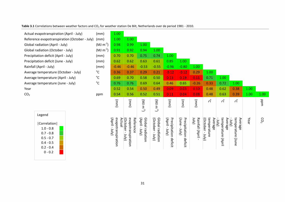
3.3.1 Correlations between factors

Very strong correlations (>80%) were found between global radiation and evapotranspiration and

between rainfall and precipitation deficit (Table 3.1 & App. I: Tables I.1-I.3). Precipitation deficit,

rainfall and average temperatures in spring and summer correlated strongly (45-80%) with global

radiation and evapotranspiration, as well average temperatures from mid-April to mid-July with

precipitation deficit.

3.3.2 Models with combined factors

Average temperature during the growing season was included in seven of the ten models with a

negative effect on yields, precipitation deficit from June to July was included in two models with a

positive effect, besides those precipitation deficit from April to July with positive effect, rainfall from

April to July with negative effects and CO2 with positive effects, were selected (Table 3.2). The

regions Oostelijk veehouderijgebied, Centraal veehouderijgebied, Westelijk Holland, Waterland &

Droogmakerijen, Rivierengebied and Zuidelijk veehouderijgebied were only influenced by weather

via the average temperature during the growing season. The regions IJsselmeerpolders,

Hollands/Utrechts weidegebied and Zuidwestelijk akkerbouwgebied were influenced by,

respectively, precipitation deficit from April to July, rainfall from April to July and precipitation deficit

from June to July. Climate effects on Zuid-Limburg included average temperature during the growing

season, precipitation deficit from April to July and CO2. The regression model for Zuid-Limburg has

unexpected coefficient values. This might be due to aliasing between CO2 concentrations in the air

and years.

-200

-100

0

100

200

300

400

500

1980 1985 1990 1995 2000 2005 2010 2015

Pre

cip

itat

ion

def

icit

& R

ain

fall

(mm

)

Year

Figure 3.7 Trends in rainfall and precipitation deficit of winter wheat (Triticum aestivum L.) accumulated

over a period of April to July (rainfall [red], precipitation deficit [green]) and June - July (precipitation deficit

[blue]) from 1981 to 2010 at De Bilt, Netherlands. In the equations x = year -1981.

31

Table 3.1 Correlations between weather factors and CO2 for weather station De Bilt, Netherlands over de period 1981 - 2010.

Actual evapotranspiration (April - July) (mm) 1.00

Reference evapotranspiration (October - July) (mm) 1.00 1.00

Global radiation (April - July) (MJ m-2) 0.98 0.99 1.00

Global radiation (October - July) (MJ m-2) 0.91 0.92 0.94 1.00

Precipitation deficit (April - July) (mm) 0.70 0.70 0.75 0.74 1.00

Precipitation deficit (June - July) (mm) 0.62 0.62 0.63 0.61 0.85 1.00

Rainfall (April - July) (mm) -0.46 -0.46 -0.53 -0.55 -0.96 -0.80 1.00

Average temperature (October - July) oC 0.36 0.37 0.29 0.21 -0.12 -0.12 0.29 1.00

Average temperature (April - July) oC 0.69 0.70 0.58 0.50 0.13 0.19 0.11 0.71 1.00

Average temperature (June - July) oC 0.76 0.76 0.69 0.64 0.46 0.65 -0.26 0.33 0.72 1.00

Year 0.52 0.54 0.50 0.49 0.09 0.03 0.10 0.48 0.62 0.38 1.00

CO2 ppm 0.54 0.56 0.52 0.51 0.11 0.04 0.08 0.48 0.63 0.39 1.00 1.00

(mm

)

(mm

)

(MJ m

-2)

(MJ m

-2)

(mm

)

(mm

)

(mm

)

oC

oC

oC

pp

m

Actu

al

evapo

transp

iration

(A

pril - Ju

ly)

Refe

rence

evapo

transp

iration

(Octo

ber - Ju

ly)

Glo

bal rad

iation

(A

pril - Ju

ly)

Glo

bal rad

iation

(O

ctob

er - July)

Precip

itation

deficit

(Ap

ril - July)

Precip

itation

deficit

(Jun

e - July)

Rain

fall (Ap

ril - Ju

ly)

Ave

rage te

mp

erature

(Octo

ber - Ju

ly)

Ave

rage

tem

peratu

re (Ap

ril - Ju

ly)

Ave

rage

tem

peratu

re (Jun

e - Ju

ly)

Year

CO

2

Legend

|Correlation| -

1.0 - 0.8

0.7 - 0.8

0.5 - 0.7

0.4 - 0.5

0.2 - 0.4

0 - 0.2

32

Table 3.2 Coefficients of multivariate linear regression analyses on relation between climate factors an winter wheat yields at 15% moisture (kg ha-1

) in the Netherlands

from 1981 - 2010 using bidirectional elimination.

Region

Model P

R2adj.

Constant

Year

Average

temperature

GSa (oC)

Precipitation

deficit

JJ b (mm)

Precipitation

deficit

AJ c (mm)

Rainfall

AJ c (mm)

CO2

(PPM)

Oostelijk veehouderijgebied 9368 98.0 -414 <.001 0.61

Centraal veehouderijgebied 9665 88.3 -487 <.001 0.53

IJsselmeerpolders 7262 71.45 4.87 <.001 0.65

Westelijk Holland 13109 -499 0.007 0.32

Waterland & Droogmakerijen 12941 -460 0.053 0.16 Hollands/Utrechts

weidegebied 9964 -8.14 0.006 0.34

Rivierengebied 10289 93.1 -419 <.001 0.67 Zuidwestelijk

akkerbouwgebied 7448 62.2 4.29 <.001 0.57

Zuidelijk veehouderijgebied 8805 79.7 -312 <.001 0.59

Zuid-Limburg 71128 411 -313 2.75 182.9 <.001 0.78

a Growing season: October - July

b June - July

c April - July

33

3.4 Calibration

3.4.1 Development

3.4.1.1 Emergence

Table 3.3 shows the model parameters before and after calibration. The adjusted relations in the

model can be found in figure 3.8 and App. I: figs I.8 and I.9.

Observed and simulated dates of emergence, start of grain filling and maturity can be found in figure

3.9. Since these dates are expressed in Julian day of the growing season, there is a difference of 365

days between crops sown before and after New Year.

Table 3.3 Original (spring wheat) and calibrated (winter wheat) values of parameters for the LINTUL winter

wheat (Triticum aestivum L.) model in the Netherlands.

Parameter Parameter in Model

Unit Original

Calibrated

Development

Tsum-emergence TSUMEM

oC day 89b

122

Tbasem TBASEM

oC 1.3b

0.25

Tb TBASE

oC 0

1.5

Tsum-anthesis TSUMAN

oC day 720

926

Tsum-maturity TSUMMT

oC day 950

590

Vsat VERSAT

Day 70

58

M MSOIL

- 0.25a

0.25

Leaf area

Tsum-ageing TSUMAG

oC day 720

900

Sla-correction SLAC

- 0.0212

0.021

rl RGRL

oC day-1 0.00817

0.015

Lcr LAICR

- 4

4

Rd-shmx RDRSHM

day-1 0.03

0.03

Maximum sink limited LAI - 0.75 0.6

Assimilate production

Wlvgi WLVGI

g m-1 0.16c

0.07

Wsti WSTI

g m-1 0.08c

0.04

LUE LUE

g MJ-1 3.00

3.15

k K

- 0.6

0.6

a Source: (Zheng et al., 1993)

b Based on an average of Angus (1980) and Bauer (1984)

c Based on data from Boons - Prins et al. (1993) and Van Heemst (1988)

34

Figure 3.9 Simulated and observed dates of emergence, start of grain filling and maturity of

winter wheat in the Netherlands in Julian day where January 1st

= 1.

0

0.2

0.4

0.6

0.8

1

1.2

0 0.5 1 1.5 2

Allo

cati

on

fac

tor

(d-1

)

Development stage

Stem - calibrated

Stem - original

Grain - calibrated

Grain - original

Roots - calibrated

Roots - original

Leaves -calibrated

Leaves - original

Figure 3.8 Original and calibrated relation between development stage and allocations factors of assimilates

to the roots, stem, leaves and grain (d-1

) of winter wheat (Triticum aestivum L.).

-150

-100

-50

0

50

100

150

200

250

300

-150 -100 -50 0 50 100 150 200 250 300

Sim

ula

ted

de

velo

pm

en

t (j

ulia

n d

ay)

Observed development (julian day)

Maturity

Start grainfillingEmergence

1:1 line

35

3.4.2 Growth

3.4.2.1 Initial plant weight

The initial weight of stem and leaves were derived from data of Boons - Prins et al. (1993) and Van

Heemst (1988). The average plant rate is 45 plants m-2 and the initial plant weight is 0.011 g plant-1

both given by Van Heemst (1988). According to Boons - Prins et al. (1993) half of the plant weight is

aboveground biomass and 65% of the aboveground biomass is in the leaves.

Initial total dry weight = 0.011 * 45 = 4.95 g m-2

Initial total aboveground biomass = 4.95 * 0.5 = 0.25 g m-2

Initial weight green leaves = 0.2475 * 0.65 = 0.16 g m-2

Initial weight stem = 0.2475 * 0.65 = 0.087 g m-2

3.4.2.2 Evaluation of calibration data

The average water content of the rooted zone only slightly went under the critical water holding

content for The Bouwing in both years (App. I: Figs I.10 I.11). For all locations the depth between the

root zone and the groundwater table never exceeded one meter after the 1st of May (App. I: Fig I.12).

36

3.4.2.3 Calibration growth

Figure 3.10 Simulated (lines) and measured (symbols) aboveground biomass [a], leaf area index [b], weight of green leaves [c], weight of death leaves [d], stem + chaff

[e], grain yields of winter wheat [f] in 1983 (red) and 1984 (green) at The Bouwing (□), The Eest (∆) and PAGV (○).

0

200

400

600

800

1000

1200

1400

1600

1800

2000

350 450 550

Ab

ove

gro

un

d b

iom

ass

(kg

ha

-1)

Julian day

0

1

2

3

4

5

6

350 450 550

LAI

Julian day

0

50

100

150

200

250

300

350 450 550

Gre

en

leav

es

(kg

ha

-1)

Julian day

0

20

40

60

80

100

120

140

160

180

200

350 450 550

De

ad le

ave

s (k

g h

a-1

)

Julian day

0

200

400

600

800

1000

1200

350 450 550

Ste

m w

eig

ht

(kg

ha

-1)

Julian day

0

100

200

300

400

500

600

700

800

900

350 450 550

Gra

in y

ield

(kg

ha

-1)

Julian day

a b c

d e f

37

There was a correlation of 30% between observed and simulated yields (Fig. 3.11). Crops with high or

low plant densities were all underestimated by the LINTUL model. There seemed to be a tendency to

overestimate low yields and underestimate high yields.

Figure 3.11 Simulated and observed yields (15% moisture) of winter wheat in

the Netherlands sown in September (yellow), October (green) and November

or later (purple), before (closed symbols) and after (open symbols) 1990,

grown at plant densities lower than 250 plants m-2

(◊), between 250 and 400

plant m-2

(○) and higher than 400 plants m-2

(□). Sources: Darwinkel, 1994;

Darwinkel, 1985; PPO Lelystad, 2012. Additional information in App. III.

R² = 0.30

5.0

6.0

7.0

8.0

9.0

10.0

11.0

12.0

5.0 7.0 9.0 11.0

Sim

ula

ted

yie

ld (

g m

-2)

Observed yield (g m-2)

38

3.5 Simulations

3.5.1 Influence of temperature change

Time of emergence (Fig. 3.12a) and duration of the period from anthesis to harvest (App. I: Fig. I.13a)

of normal sown winter wheat did not show a significant (F > 0.05) trend over time. Time of anthesis

and harvest (Fig. 3.12a) both declined linearly (P < 0.05), with 0.37 and 0.48 days year-1 or 11 and 14

days in 30 years, respectively. The duration of the period between emergence and harvest also

declined, with 0.35 days year-1, i.e. 10 days in 30 years (App. I: Fig. I.13a). Time of emergence and

anthesis (Fig. 3.12b) and duration of the periods from emergence to anthesis and the period from

anthesis to harvest (App. I: Fig. I.13a) of late sown winter wheat did not show a significant (P < 0.05)

trend over time. The time of harvest did decline with 0.41 days year-1 or 12 days in 30 years (App. I:

Fig. I.13a). The deviation between the longest day (21 June) and the median day of the period from

anthesis to harvest decreased linearly (P < 0.05) from 1981 to 2010 for both sowing dates (App. I: Fig.

I.13b). The magnitudes of decrease were 0.34 and 0.41 days per year i.e. 10 and 12 days in 30 years.

The cumulative incoming global radiation during the period from emergence to anthesis decreased

linearly (P < 0.05) with 6.63 and 7.06 KJ m-2 year-1 for, respectively, normal and late sown winter

wheat from 1981 to 2010 (Fig. 3.12c). For the period after anthesis cumulative incoming global

radiation did not show a significant trend for both sowing dates (Fig. 3.12c). The average value of the

LUE correction factor for mean daily temperature only showed a significant (P < 0.05) trend for the

period of emergence to anthesis of normal sown winter wheat (App. I: Fig. I.13b). No significant

change was found for the period after anthesis of late sown winter wheat and for both periods of the

normal sown crop.

For both ‘varieties’ and sowing dates of winter wheat no significant (P < 0.05) trend in simulated total

aboveground biomass at anthesis and harvest, grain yields and harvest index, were found over the

period 1981-2010 (App. I: Figs. I.14 & I.15).

3.5.2 Influence of radiation change

Total incoming global radiation before anthesis increased linearly (P < 0.05) with 12.3 and 11.9 kJ m-2

per year from 1981 to 2010, for normal and late sown winter wheat respectively (Fig. 3.14a). No

significant trend was found for total incoming global radiation after anthesis (Fig. 3.14a)

The grain yield and total aboveground biomass at anthesis and harvest increased linearly from 1981

to 2010 for both varieties and sowing dates (Fig. 3.14b, App. I: Table I.5) No significant (P < 0.05)

trend was found for the harvest index of winter wheat for all varieties and sowing dates (Fig. 3.14c,

App. I: Table I.5)

0

39

∆y = 4.27*10-3x R2 = 0.19

0.40

0.60

0.80

1.00

1.20

1980 1985 1990 1995 2000 2005 2010 2015

Co

rre

ctio

n f

acto

r o

f L

UE

fo

r d

ay

tem

pe

ratu

re

Year

Normal sown - emergence until anthesisLate sown - emergence until anthesis

*

a

c

R² = 0.39; ∆y = -0.483x

R² = 0.30; ∆y = -0.374x

250

300

350

400

450

500

550

600

650

1980 1985 1990 1995 2000 2005 2010 2015

Tim

e (

day

of

year

+ 3

65

)

Year

Harvest Anthesis Emergence

R² = 0.27; ∆y = 6.63x

R² = 0.32; ∆y = 7.06x

0

500

1000

1500

2000

2500

1980 1985 1990 1995 2000 2005 2010 2015C

um

mu

lati

ve r

adia

tio

n (

kJ m

-2 )

Year

Normal sown - anthesis to harvest Late sowing - anthesis to harvest

Normal sown - emergence to anthesis Late sown - emergence to anthesis

*

R² = 0.15; ∆y = -0.407x

250

300

350

400

450

500

550

600

650

1980 1985 1990 1995 2000 2005 2010 2015

Tim

e (

day

of

year

+ 3

65

)

Year

Harvest Anthesis Emergence

*

*

a

*

*

a

Figure 3.12 Simulated time of emergence, anthesis and harvest normal (10 October) [a] and late (25 November) [b] sown winter wheat, based on average data for radiation and annual average CO2

levels over the period of 1981 to 2010 and actual

minimum and maximum temperatures, using the LINTUL model. In the equations of the relationships x is in years with x = 0 year - 1981. ∆ stands for the slope of a trend. Data series marked with an * do not show a significant (P < 0.05) trend. Additional information can be found in Appendix I, Table I.4

c b

0

0

0

0

Figure 3.13 Simulated average correction factor for LUE [a] and cumulative radiation [b] during simulated crop stages of normal (10 October) and late (25 November) sown winter wheat, based on average data for radiation and annual average CO2

levels over

the period of 1981 to 2010 and actual minimum and maximum temperatures, using the LINTUL model. In the equations of the relationships x is in years with x = year - 1981. ∆ stands for the slope of a trend. Data series marked with an * do not show a significant (P < 0.05) trend. Additional information can be found in Appendix I, Table I.4

40

R² = 0.44 ∆y = 0.151x

R² = 0.46 ∆y = 0.129x

R² = 0.21 ∆y = 0.0659x

5

10

15

20

25

30

1980 1985 1990 1995 2000 2005 2010 2015

Ab

ove

gro

un

d b

iom

ass

(Mg

ha

-2)

Year

Aboveground biomass - Harvest Aboveground biomass - Anthesis Grain

R² = 0.49 ∆y = 12.3x

R² = 0.48; ∆y = 11.9x

0

500

1000

1500

2000

2500

3000

1980 1985 1990 1995 2000 2005 2010 2015

Cu

mm

ula

tive

rad

iati

on

(M

J m

-2 )

Year

Normal sown - anthesis to harvest Late sown - anthesis to harvestNormal sown - emergence to anthesis Late sown - emergence to anthesis

*

0.35

0.40

0.45

0.50

0.55

1980 1985 1990 1995 2000 2005 2010 2015

Har

vest

In

de

x

Year

Figure 3.14 Cumulative radiation during simulated crop stages of normal (10 October) and Late (25

November) sown winter wheat [a] simulated aboveground biomass (DM) at anthesis and harvest and grain

yield (15% moisture) [b] and harvest index [c] of a normal sown (10 October) winter wheat crop in the

Netherlands, based on daily temperatures and annual CO2 concentrations averaged over the period 1980 -

2010 and actual daily radiation levels using the LINTUL1 model calibrated for the early 1980’s . Equations of

the relationships are described in table I.5. ∆ stands for the slope of a trend. Data series marked with an *

do not show a significant (P < 0.05) trend.

*

0

0

a

b

c

0

41

R² = 1.0 ∆y = 0.134x - 2.07*10-3x2

∆y = 0.100x - 1.55*10-3x2

R² = 1.0

∆y = 0.0621x - 9.62*10-4 x2

R² = 1.0

5

10

15

20

25

1980 1985 1990 1995 2000 2005 2010 2015

Ab

ove

gro

un

d b

iom

ass

(Mg

ha

-2)

Year

Aboveground biomass - Harvest aboveground biomass - Anthesis Grain

R² = 1.0 ∆y = 5.5*10-3x - 8.55*10-5x2

0.90

0.95

1.00

1.05

1.10

1980 1985 1990 1995 2000 2005 2010 2015

CO

2 co

rre

ctio

n f

acto

r fo

r LU

E

Year

R2 = 1.0 ∆y = 2.97*10-4x - 4.82*10-6x2

0.35

0.40

0.45

0.50

0.55

1980 1985 1990 1995 2000 2005 2010 2015

Har

vest

In

de

x

Year

Figure 3.15 Simulated value of correction factor for the LUE of winter wheat crops in the Netherlands,

based on CO2 concentrations in the air [a] simulated aboveground biomass (DM) at anthesis and harvest

and grain yield (15% moisture) [b] and harvest index [c] of a normal (10 October) sown winter wheat crop in

the Netherlands, based on average weather data from 1980 to 2010 and actual CO2 levels in the air using

the LINTUL1 model calibrated for the early 1980’s In the equations of the relationships x is in years with x =

0 for the year 1981. ∆ stands for the slope of a trend. Data series marked with an * do not show a

significant (F < 0.05) trend. Additional information can be found in table I.6

a

b

c

0

0

0

42

3.5.3 Influence of CO2 change

The average LUE correction factor for CO2 showed a quadratic trend (P < 0.05) with a diminishing

increase from 1981 to 2010 (Fig. 3.15a). As a result the grain yield and total aboveground biomass at

anthesis and harvest showed a similar trend over the period 1981 - 2010 for both varieties and

sowing dates (Fig. 3.15b, App. I: Table I.6). The harvest index showed an opposing quadratic trend

over that period, the trend was a diminishing decline (3.15c, App. I: Table I.6)

3.5.4 Influence of actual weather

Time of emergence (Fig. 3.12a) and duration of the period from anthesis to harvest (App. I: Fig.

I.13a) of normal sown winter wheat did not show a significant (P < 0.05) trend over time. Time of

anthesis and harvest (Fig. 3.12a,b) of both declined linearly (P < 0.05), with 0.37 and 0.48 days year-1

or 11 and 14 days in 30 years, respectively. The duration of the period between emergence and

harvest also declined, with 0.35 days year-1 i.e. 10 days in 30 years (App. I: Fig. I.13a). Time of

emergence and anthesis (Fig. 3.12b) and duration of the periods from emergence to anthesis and

from anthesis to harvest (App. I: Fig. I.13a) of normal sown winter wheat did not show a significant (P

< 0.05) trend over time. The time of harvest did advance earlier with 0.41 days year-1 or 12 days in 30

years

For late sown winter wheat a significant (P < 0.05) positive quadratic trend in total incoming global

radiation was found for the period between anthesis and harvest (App. I: Fig. I.16a). Total incoming

global radiation did not change significantly after anthesis for normal sown winter wheat and before

anthesis for both sowing dates (App. I: Fig. I.16b).

The aboveground biomass at anthesis and harvest shows a significant linear trend for normal sown

and quadratic trend for late sown winter wheat (Fig. 3.16a,b). The difference between normal and

late sown winter wheat is explained by the effect of the LUE correction factor due to temperature

change (Fig. 3.13a). The grain yield of both models and sowing dates shows a quadratic trend (Fig.

3.17a). This trend can be explained by the quadratic effect of the CO2 concentrations on the LUE

combined with the quadratic effect on total biomass of late sown winter wheat. The harvest index

decreases for both varieties and sowing dates with 0.03 to 0.05 over 30 years (Fig. 3.17b).

43

R² = 0.52; ∆y = 0.163x

R² = 0.58 ∆y = 0.211x

R² = 0.52 ∆y = 0.171x

R² = 0.58; ∆y = 0.222x

5

10

15

20

25

30

1980 1985 1990 1995 2000 2005 2010 2015

Ab

ove

gro

un

d b

iom

ass

(Mg

DM

ha

-2)

Year

Anthesis - V1 Harvest - V1Anthesis - V2 Harvest - V2

R² = 0.13 ∆y = -9.98*10-4x

R² = 0.15

∆y = -1.32*10-3x

R² = 0.17 ∆y = -1.13*10-3x

∆y = -1.50*10-3x R² = 0.20

0.35

0.40

0.45

0.50

0.55

0.60

0.65

1980 1985 1990 1995 2000 2005 2010 2015H

arve

st I

nd

ex

Year

Normal sown - V1 Late sown - V1

Normal sown - V2 Late sown - V2

∆y = 0.467x - 0.0102x2

R² = 0.50

R² = 0.56 ∆y = 0.583x - 0.123x2

∆y = 0.492x - 0.0107x2 R² = 0.50

∆y = 0.605x - 0.127x2

R² = 0.56

5

10

15

20

25

30

1980 1985 1990 1995 2000 2005 2010 2015

Ab

ove

gro

un

d b

iom

ass

(Mg

ha

-2)

Year

Anthesis - V1 Harvest - V1Anthesis - V2 Harvest - V2

∆y = 0.204x - 0.00412x2

R² = 0.61

R² = 0.63; ∆y = 0.278x - 0.006063 x2

R² = 0.64; ∆y = 0.250x - 0.00508x2

R² = 0.64 ∆y = 0.324x - 0.00703x2

6

8

10

12

14

16

1980 1990 2000 2010

Gra

in 1

5%

mo

istu

re (

Mg

ha

-2)

Year

Normal sowing - V1 Late sowing - V1

Normal sowing - V2 Late sowing - V2

3.16 Simulated aboveground biomass at anthesis and harvest of normal (10 October) [a] and late (25 November) [b] sown winter wheat, based on real weather data using the LINTUL model calibrated for the early 1980’s (V1) and a model adjusted to varieties around 2010 (V2). In the equations of the relationships x is in years with x = year - 1989. ∆ stands for the slope of a trend. Data series marked with an * do not show a significant (P < 0.05) trend. Additional information can be found in table I.7

a

0

0

0

0.00

a

b

a

b

3.17 Simulated grain yield (15% moisture) [a] and harvest index [b] of normal (10 October and late (25 November) sown winter wheat, based on real weather data using the LINTUL model calibrated for the early 1980’s (V1) and a model adjusted to varieties around 2010 (V2). In the equations of the relationships x is in years with x = year - 1989. ∆ stands for the slope of a trend. Data series marked with an * do not show a significant (P < 0.05) trend. Additional information can be found in table I.7

44

4 Discussion

4.1 Yield The yield trend analysis showed that there was no stagnation in growth of winter wheat yields from

1981 to 2010 in the Netherlands both at national and regional level. This was also found by Rijk

(2013). The analyses of national yield trends starting between 1970 and 1977 up to 2010, however,

showed a quadratic trend, suggesting a levelling off of the yields indeed. This would be in accordance

with findings of Brisson et al. (2010) and Petersen et. al. (2010) who found that yields in the

Netherlands stagnated after 1993. However, it is important to notice that Brisson et al. (2010) and

Petersen et. al. (2010) used data from the FAO instead of CBS and that they investigated yields over a

period of ± 1960 to 2007. Also for most other countries in Europe stagnation of yield growth was

found or suggested, namely France (Brisson et al., 2010; Calderini and Slafer, 1998; Petersen et al.,

2010), United Kingdom (Knight et al., 2012; Brisson et al., 2010; Calderini and Slafer, 1998; Petersen

et al., 2010), Denmark (Slafer and Peltonen-Sainio, 2001; Brisson et al., 2010; Petersen et al., 2010),

Switzerland (Finger, 2010; Brisson et al., 2010), Finland (Slafer and Peltonen-Sainio, 2001; Peltonen-

Sainio et al., 2009), Sweden (Batts et al., 1996; Petersen et al., 2010), Belgium (Petersen et al., 2010)

and Norway (Slafer and Peltonen-Sainio, 2001). The only North-Western European country which is

not experiencing yield stagnation in winter wheat seems to be Germany (Brisson et al., 2010;

Calderini and Slafer, 1998), although Petersen (2010) suggests there is has been no yield increase

after 1998. Also on world scale there are indications of stagnation of winter wheat yields. Already in

1998 Calderini & Slafer found signs for this in 65% of the wheat growing areas.

45

4.2 Area The national cultivated area of winter wheat did not change, even though some regional cropped

areas did change. Also for other countries in Europe the area of winter wheat did not change for this

period. Petersen et al (2010) found that the total area of wheat cultivation has been more or less

stable since the 1970’s for Belgium, Germany, Netherlands, Sweden and France (also found by

Brisson et al (2010)). Both Petersen et al (2010) and Calderini & Slafer (1998) found that the cropped

area in UK was still rising in the beginning of the 1980’s but did not change after 1990.

Figure 5.1 Soil map of the Netherlands with agricultural regions according to CBS after 1990.

46

The changes in regional areas cropped with winter wheat show that in a lot of sandy regions area

increased, while in regions with clayey or loamy soils the areas decreased (Fig. 5.1 and App. I.1,2).

Yields in the sandy regions Oostelijk veehouderijgebied, Centraal veehouderijgebied and Zuidelijk

veehouderijgebied are on average 18% lower than the national yield per ha. Therefore these changes

might make the average national yields decline, due to the growing influence of the sandy areas.

However, the cumulative increase of the cultivated area in these regions, including Zuidwest Brabant,

is 9,193 ha from 1981 to 2010, which is 8% of the average total national area. This means that the

influence of this area change is a only 1.4% decrease in the national yield over the period of 1981 to

2010. Calderini & Slafer (1998) also concluded that changes in national yields per ha around the

world were not caused by changes in area.

4.3 Climate effects

4.3.1 Changes in climate

The CO2 concentrations in the air shows an accelerated increase (Fig. 3.3). This is in agreement with

findings of IPCC assessments (Forster et al., 2007) which found that the rate of increase of CO2 from

1995 to 2005 was the highest rate during any decade since 1950 until then.

Average annual and seasonal temperatures in the Netherlands increase all over the country (Fig. 3.4).

This is confirmed by the KNMI in its report on the state of the climate in the Netherlands in 2008

(Kattenberg, 2008). Kattenberg (2008) states that temperatures in the Netherlands and a large part

of western Europe increased twice as fast as the world average temperature since 1950. Specific

reasons for this in the Netherlands are the trend towards a more westerly wind in late winter and

early spring which brings in relatively warm air from above the sea and an increase in global radiation

in spring and summer. Bresser et al. (2005) state that the prevailing wind directions are hard to

predict on the long term, so current changes might be altered in the future. Over the period of 1950

to 2008 the increase in spring and autumn temperatures is respectively 2.8 and 1.8 times faster than

the global average increase (Bresser et al., 2005). The difference between spring and autumn occurs

because the previously mentioned processes, which contribute to the faster increase, occur in the

first half of the year. This can be important for the effect of temperature changes on plant growth.

One of the reasons for higher temperatures is increasing incoming radiation as was also described in

the results (Fig. 3.5). The radiation increased during the whole growing period of winter wheat and

during the period from April to July. Kattenberg (2008) also mentions this increase and the reasons

for it. Until about 1985 there was a small decrease of radiation in spring and summer, after that

there was a strong increase. The first reason for increase in incoming global radiation is the

brightness of the atmosphere. Until the 1980’s the amount of aerosols in the air increased, from the

second half of the 1980’s the air became cleaner again, so more solar radiation reached the ground.

The other reason which is more important in the long run is the change in overcast. In spring and

summer the overcast is reducing with warmer easterly and southerly wind. Also for Denmark

(Petersen et al., 2010) and the UK (Knight et al., 2012) increases in sunshine hours were reported.

Due to the increase in temperature and radiation the potential evapotranspiration of winter wheat

increases in the Netherlands (Fig. 3.6), despite the slight reduction in average wind speed mentioned

by Kattenberg (2008). Since there is no significant increase in average precipitation between April

and June (Fig. 3.7), precipitation deficit would logically go up. However due the large variation in

average precipitation from April to July there is no significant trend in average precipitation deficit in

47

late autumn and early summer. With respect to this Kattenberg (2008) found no trend in maximum

precipitation deficit between 1906 and 2007.

4.3.2 Effects of changes in climate

The negative correlation between average temperature during the growing season and winter wheat

yields in the Netherlands (Table 3.2) is a relation that is often found for wheat in Western Europe

(Petersen et al., 2010). The most likely explanation for this is that due to higher temperatures the

growing period shortens (Petersen et al., 2010; Knight et al., 2012). This means that there is also less

time for intercepting radiation which results in lower yields. Another explanation mentioned by

Petersen et al. (2010) is that in years with high temperatures there is more radiation and less rain

which leads to water shortage during anthesis. However this explanation seems not very plausible

since there are low correlations between average temperature during the growing season and

rainfall in spring and early summer (Table 3.1) and rainfall is negatively correlated with yield while

precipitation deficit has a positive influence (Table 3.2). Since the regression model includes the

average temperature over the growing period and not only from April or June to July, it seems that

temperatures from autumn to spring were also important. With respect to this Kristensen et al

(2011) found that winter temperatures in Denmark significantly correlated with yield. On the one

hand they noticed the abovementioned negative effect of high winter temperatures on the growing

period. On the other hand they recorded a negative effect of very low winter temperatures on yield,

probably caused by frost damage to the plants or drought problems due to reduced root

development in winter. The reducing effect of frost was also found by Knight et al. (2012), who

recorded a negative impact of the number of frost days on winter wheat yields. Kristensen et al

(2011) also found a negative effect of temperature on winter wheat yields in summer. Since this

effect was higher on sandy soils it is likely related to water shortage during grain filling, because

these soils have a lower water holding capacity.

The positive correlation between precipitation deficit and winter wheat yields cannot be a direct

effect, since normally precipitation deficit means water shortage. However, the correlations show

that precipitation deficit is highly correlated with rainfall as well as radiation. Therefore a high

precipitation deficit could stand for low amounts of rainfall or high amounts of radiation which could

lead to increasing yields. The negative correlation between the cumulative rainfall from April to July

and wheat yields in Hollands/Utrechts weidegebied confirm the explanation that low amounts of

rainfall can be improving yields. Similar relations between rainfall were found for winter precipitation

in Denmark (Petersen et al., 2010). Petersen et al. (2010) state that the negative effect of winter

precipitation can be caused by low nitrogen availability due to leaching or reduced root development

due to drainage problems. Negative impacts of summer rainfall on yields could be increases in

diseases, like Fusarium spp. which develop faster under humid circumstances, damage due to lodging

and harvest losses on soils with bad drainage. Drainage problems are a likely explanation for the

findings in the Netherlands, since the negative correlations with rainfall were not found in sandy

areas. Chloupek et al.(2004) and Brown (2013) also found high wheat yields in dry and warm

summers in the Czech Republic and Scotland respectively. Besides that they measured that there was

more sunshine during these summers, supporting the reasoning that high precipitation deficit is

related to high levels of radiation. The results show that apparently drought is not a big problem in

the Netherlands (Table 3.2). Kristensen (2011) and Petersen (2010) concluded the same for Denmark,

although it is important to notice that winter wheat on sandy soils in Denmark is often irrigated.

48

4.3.3 Modelling

4.3.3.1 Modelling assumptions and choices

In this model the relation between the CO2 concentrations in the air and the LUE an arbitrary

function generation (AFGEN) function was used. This function does linear interpolation, while a

smoothing spline interpolation might be a more realistic representation of the relation in reality,

since it does not contain sudden changes in the slope of the relation at the interpolation points.

In the spring wheat model reallocation was simulated by starting allocation of assimilates to the

grains before anthesis, which is not in accordance with reality. To avoid this the reallocation module

was inserted in this version of the model. However, the development stage at which grain filling

started was chosen too late (zadoks scale: 71, feekes scale: 10.54; Kernel watery ripe). Zadoks scale

65 (Anthesis half-way) might have been more appropriate since the data from Groot en Verberne

(1991) showed that the wheat crop already had grain weight when it reached zadoks scale 65.

Due to the late timing of the start of grain filling, reallocation had to start before DVS =1 to simulate

the measured trend in grain biomass build up.

The validation data show that there is not a very high correlation between observed and simulated

yields, especially not if the outliers to the upper right are not taken into account (Fig. 3.11). This is of

course very important, since a model that does not represent reality very well is a weak basis to build

conclusions on. There are two possible reasons for the low correlation. Firstly, the assumption that

the validation data represents optimal potential crop growth and yield, might be wrong. This could

be the case, since for all data from Darwinkel (1994; 1985) it is not known if disease control was used

or if crop yields were reduced in any way. Besides that, there were differences in yields of crops

grown at the same location and same sowing dates. As explained before the lower yields were

removed in those cases, since they clearly did not represent optimal yield. However, the fact that

those yields were reduced, imply that the highest yields, which were kept as validation data, could

also be non-optimal.

The second reason is of course the model itself. The model seems to be very inaccurate for low or

high plant densities. For in the graph (Fig. 3.11) the yields from crops sown at densities between 250

and 400 plants m-2 are scattered much more around the 1:1 line, than those from higher or lower

densities, which are all below the 1:1 line. Besides that, the yields from crops sown in September are

also all at the right side of the 1:1 line. This suggests that the model underestimates the positive

effect of early sowing on yields. These limitations of the model should be kept in mind while judging

the outcomes. Although these outcomes have not to be completely rejected, it might be necessary to

focus more on the global trends than on very specific details.

To evaluated the effect of individual weather factors, simulations where carried out with averaged

daily weather data over 30 years. This is not without consequence. Since the data is average all

extreme daily values are weakened. For temperatures extremely high or low temperatures mostly

result in suboptimal growing conditions and thus reduced yields. So the simulations with averaged

weather data might in general give an overestimation of yields compared to reality. This might

explain why cumulative increase in biomass of all individual factors is higher than the biomass

increase due to the combination of all three factors in this research.

49

4.3.3.2 Modelling results

Since development of winter wheat is temperature dependent, the measured increase in average

temperature over the growing season leads to faster development of the crop. This effect comes

back in nearly every study on the effect of climate on wheat yields (Nonhebel, 1993; Olesen et al.,

2000; Ghaffari et al., 2002; Wolf et al., 1996; Estrella et al., 2007; Olesen and Bindi, 2002;

Schapendonk et al., 1998; Børgesen and Olesen, 2011; Tonkaz et al., 2010; Petersen et al., 2010).

With a temperature increase of 1.3 to 1.6 oC, harvest dates became 12 to 14 days earlier over 30

years. This effect is stronger than the 4.4 to 5.2 day per oC estimated by Estrella et al. (2007) in

Germany, the 6 and 10 days for 0.9 and 1.5 oC respectively found by Ghaffari et al. (2002) and the 15

to 20 days for 3 degrees mentioned by Nonhebel (1993). An even stronger effect was mentioned by

Petersen et al. (2010) for Denmark, namely 5% per 1 degree change.

The shift in phenology of winter wheat in the Netherlands to earlier harvest leads to a reduction in

interception of radiation before anthesis in two different ways (Nonhebel, 1993). Firstly the growing

season and thus the time to intercept radiation becomes shorter. Secondly the growing period shifts

more towards winter during which radiation levels are lower. This process results in lower yields

(Olesen et al., 2000; Tonkaz et al., 2010; Olesen and Bindi, 2002; Petersen et al., 2010). It is important

to notice that there was no significant change in global radiation during the period of grain filling.

Besides that the shift in phenology means that the period of grain filling is ‘timed’ more around the

longest day. So the radiation levels during this period might even increase.

Besides development, temperature also affects assimilation rate (Nonhebel, 1993). If mean daily

temperatures are lower than 12 oC the LUE is suboptimal. In the period before anthesis, spring, there

are many suboptimal days resulting in an average LUE correction factor for temperature which is

lower than 1. This study shows that this LUE correction factor is increasing over the years due to

higher mean temperatures. This results in a higher LUE and higher assimilation and growth. So higher

temperatures during cold phases of the growing period are increasing growth and yield

(Schapendonk et al., 1998). This was also found for Denmark by Olesen et al. (2000) and for

simulated winter wheat in the UK by Wolf et al. (1996). Higher average temperatures in winter can

also be positive because it indicates less frost damage; however frost damage was not included in

this study. Olesen et al. (2000) found that higher yields in Denmark due to higher winter

temperatures was most likely the effect of better establishment of the leaf area instead of better

winter survival.

In this study the positive and negative effects of higher mean temperatures during the growing

season of winter wheat are apparently counterbalancing each other, since there is no significant

change in grain yields due to temperature change. Kristensen et al. (2011) also found that

temperatures from April to June did not affect yields. Olesen et al. (2000) show that winter wheat

yields in Denmark on loamy soils slightly increase or stay stable with an increase of mean

temperature up to 3 oC and start decreasing if temperature becomes higher than 3 oC. Nonhebel

(1993) stated that the negative effect of temperature on development would be overruling other

effects and Schapendonk et al. (1998) and Nonhebel (1993) even found this for the Netherlands in an

analyses of climate change effects on winter and spring wheat yields in the future respectively.

Therefore in the future the balance in the effects might become negative since the beneficial effect

on LUE will become saturated and the effect on phenology will continue.

50

The increase of incoming global radiation over the growing season, especially before anthesis, leads

to increase assimilate production and thus biomass production of about 20% in 30 years. As

mentioned earlier part of the radiation change is due to reduction in human emitted aerosols, which

can be expected to sustain. A more important influence however is the effect of warm winds on

cloudiness. It is not clear how the overcast will change in the future which makes it hard to estimate

the changes in radiation in the coming decades.

51

4.3.4 CO2 effect

The increase in CO2 concentrations in the air causes a higher light use efficiency (Olesen and Bindi,

2002; Petersen et al., 2010; Børgesen and Olesen, 2011) and thus increased biomass production

before and during grain filling, which is found in many studies with different models (Wolf et al.,

1996; Gervois et al., 2008; Nonhebel, 1993).

The increase in yield is higher than many other studies indicate namely ± 10% with a CO2

concentration rise of 50 ppm in 30 years. Nonhebel (1993) estimated an increase of 40 to 50% with a

doubling of CO2 levels from 350 to 700 ppm. Bresser states that a doubling of CO2 concentrations can

increase yields with 15 to 20% and Tonkaz et al. (2010) estimate a yield increase of 150 kg per ha per

40 ppm increase in CO2 concentrations. Based on results from Olesen & Bindi (2002), Petersen et al.

(2010) estimate the effect of the 30 ppm increase in CO2 concentrations from 1990 to 2008 in yields

to be about 4% and Knight et al. (2012) conclude that a 50 ppm increase in CO2 concentration

results in 6% extra yield.

There are two possible reasons for the difference in yield response between this study and others.

Firstly the relation between LUE and CO2 concentrations that was used in this study is nonlinear,

which means that the LUE increase due to higher CO2 concentrations is slowing down with higher

concentrations. The nonlinear response curve of yield to CO2 levels is in agreement with results from

Olesen & Bindi (2002) and Ko et al. (2010). Since many of the above mentioned studies look at the

effect of CO2 increase in the future, when CO2 levels are higher, the relative effect of CO2 increase on

LUE is lower in those studies since the effect is reducing.

Secondly the response curve of LUE to CO2 concentrations in this study might have been

overestimating the stimulating effect of increasing CO2 levels. The response curve that is used

increases the initial LUE with 11% and the saturated LUE with 60% for a doubling of CO2 from 360 to

720 ppm, which leads to a LUE increase of 35%. This response curve is based on Supit et al. (2012),

who based their LUE adjustments on findings from the 1980’s by for instance Cure & Acock (1986).

Later Long et al. (2006) carried out free-air concentration enrichment (FACE) experiments in which

they found wheat photosynthesis responses to CO2 increase which were almost 40% lower than

those of Cure & Acock (1986), who found a 21% increase in photosynthesis if CO2 concentrations

were elevated to 550 ppm. This might explain the difference with other estimates and simulation

results. Wang et al. (2013) also found that yield increases due to elevated CO2 were lower in FACE

experiments and that many physiological factors affect the CO2 effect on plant growth. They suggest

that more detailed FACE experiments will have to create more clarity on the relation between CO2

and wheat yields.

Even though the effect might be overestimated, still it is clear that the CO2 concentration changes

over the past 30 years have led to a non-linearly increasing potential yield of winter wheat.

The decrease in HI due to higher CO2 concentrations in the air, found in this study, was also found by

Tonkaz et al. (2010) for Bulgaria. This might be due to the fact that the extra biomass production due

to the higher LUE is mostly produced during the vegetative phase of the crop growth, since in spring

there are much more days with suboptimal temperatures.

52

4.3.5 Combined effect

The overall effect of changes in weather on winter wheat yields in the Netherlands from 1981 - 2010

was positive. The potential yield of aboveground biomass and grain has increased. Grain yields

increased with 26 to 39% depending on the sowing date and variety. Petersen et al. (2010) estimate

that there was a negligible effect of weather on winter wheat yields the past decades, but that CO2

increases lead to a higher potential yield in Denmark. For the UK, Knight et al. (2012) state that there

was a positive effect of both CO2 and weather on winter wheat yields up to 1996, after that only CO2

changes continued to be positive while weather changes were negative for potential yields. Overall

the negative influence of weather after 1996 was bigger than the positive effect of CO2 increase in

the UK. Another study in the UK Ghaffari et al. (2002) found that a temperature increase of 0.9 oC

combined with a CO2 level of 400 ppm would give an 8% increase in grain yields. Supit et al. (2010)

found increasing potential yields for the Netherlands, Belgium, Germany and the UK, with 50, 40, 40

and 60 kg ha-1 year-1 from 1976 to 2005, while only incorporating radiation and temperature changes.

Although potential grain yields are increasing the response is non-linear and after the year 2000 the

increase has almost stagnated. This is mostly due to the nonlinear response of photosynthesis rates

to CO2 increases.

Changes in CO2, global radiation and temperature lead to a decline in harvest index of winter wheat.

None of the single atmospheric factors showed a significant negative effect on harvest index which

was as big as the combined effect. This suggests that the separate factors negatively influenced the

HI, although not significantly, and that the combination of these small effects resulted in a significant

decline of HI. The decline in HI probably occurs because the period before grain filling benefits more

from increased radiation, CO2 and a higher LUE than the period after anthesis. Tonkaz et al. (2010)

also found a negative effect of climate on the HI of a simulated winter wheat crop. This decline in HI

suggests that the extra assimilates produced due to atmospheric changes do not all result in extra

grain yield due to a sink limitation. With respect to this Wang et al. (2013) recommend wheat

breeders to focus on increasing the sink of wheat varieties.

4.4 Drivers of yield trends The purpose of this research was to find out what has driven yield changes in winter wheat over the

past 30 years. In figure 5.2 the yield trends at different levels are visualized. The first year of our

investigation, 1981, is taken as the point of reference to show yield changes. The change in winter

wheat yield from variety trials is derived from Rijk et al. (2013). This change can be split up in a

genetic yield change due to breeding and a yearly yield change due to other factors. In the present

study the yield change due to changes in weather, including CO2, temperature and radiation, have

been investigated. Furthermore, the trends in on-farm yields since 1981 or since before 1978

described in section 3.1.2 are included.

53

The yield change over 30 years due to genetic improvements and changes in weather could have

been five ton per ha. The change in the actual yields in the variety trials over that same period is

about 3.8 ton per ha and on farm this is only three tons. So, apparently two yields gaps have been

widening. Firstly, there was an increase in the yield gap of ± 1.3 ton per ha between potential yields

and yields in the variety trials from 1981 to 2010. Using the G x E x M concept, this means that the

environment must have caused this increase in the yield gap, since G is incorporated in both yield

trends and management of the variety trials has not changed. Secondly, the yield gap between yields

of the variety trials and on-farm yields increased with 1.7 ton per ha over the same period. Rijk et al

(2013), found a higher increase in on-farm yields, probably, due to the fact that they investigated

marine clay areas, which have a higher yield than the average national yield in this study (App. I: Fig.

I.3). Therefore, they found a smaller increase in yield gap between winter wheat on farms and in

variety trials, namely 1.2 ton per ha in thirty years. Weather influences both farm en variety trial

yield trends similarly. The genetic increase should also be the same, because farmers are likely to use

the latest varieties. Therefore the difference between farm yields and yields from trials is probably

mostly attributable to changes in management of the farmers. There are many different processes

that might have contributed to the increasing yield gaps.

4.4.1 Extreme events

In this study the direct effect of CO2 and weather on growth and development of winter wheat have

been addressed. There are, however, more effects of changes in weather patterns that have not

been addressed. Firstly extreme weather events can damage crops and thus crop yields Olesen

(2002; Bresser et al., 2005). Schaap et al. (2011) mention the following events as damaging for winter

wheat (Table 5.1):

Figure 5.2 Changes in winter wheat yield components (15% moisture) in the Netherlands from 1981 to 2010.

Yield trends from variety trials were based on Rijk et al.(Rijk et al., 2013)

-4

-3

-2

-1

0

1

2

3

4

5

6

1980 1985 1990 1995 2000 2005 2010

Gra

in y

ield

ch

ange

(M

g h

a-1

)

Year

Genetic + Weather

Genetic + year(variety trials)Weather

Genetic (Variety trials)

On-farm since <1978

On-farm since 1981

Other factors since<1978Other factors since1981

54

Schaap et al. (2011) found that the frequency of damaging extreme events will increase in the future

and this is confirmed by Kattenberg (2008). If this increase has already been started this could have

already started to negatively influence yields over the past 30 years. The measured negative

correlation between precipitation and wheat yields also indicates that damage due to wetness or

humidity in late spring and early summer have been reducing crop yields from 1981 to 2010.

Analyses in other European countries also indicate that damaging events can be significantly

influencing winter wheat yields. Knight et al. (2012) found that increasing frost in January probably

has a negative effect on winter wheat yields.

Kristensen et al. (2011) suggest that negative influences of low winter temperatures or high summer

precipitation can be due to frost damage or problems with harvesting and septoria and fusarium

diseases. In warmer countries like France, heat stress during grain filling is an important damaging

event (Brisson et al., 2010).

4.4.2 Ozone

Other processes that might have influenced winter wheat yields in the Netherlands are ground level

O3 concentrations and UV-B radiation. According to CBS et al. (2013) the exposure of vegetation to

damaging concentrations of ground level ozone declined from 1990 to 2000. After 2000 the decline

stopped. Because measurements started in the 1990’s it is not clear what happened before 1990,

although it is assumable that ozone concentrations were higher since regulations for ozone reduction

were introduced in the late 1980’s (Kattenberg, 2008). Kattenberg (2008) states that although local

emissions of ozone enhancing gasses have been reduced, background ozone concentrations are

increasing due to increases of emissions in Eastern-Asia and climatic interactions. For crop damage

peak concentrations are more important than average concentrations. Therefore the reduction in

local emissions has been more important until now and it is likely that ozone damage did not

increase over the past 30 years. For Denmark (Petersen et al., 2010) and the UK (Knight et al., 2012),

similar results were found. Besides the direct effect of reduction in peak ozone concentrations, there

is also an effect of O2 on O3 damage. Increasing O2 concentrations lead to less uptake of O3 and thus

to less internal damage(Petersen et al., 2010; Schapendonk et al., 1998). It is not clear what the

magnitude of this effect on yield has been, but it strengthens the idea that ozone damage has not

increased over the past 30 years.

Table 5.1 Damaging weather events for winter wheat in the Netherlands based on Schaap et al. (Schaap et al., 2011)

Climate factor Vulnerable period Impact on Crop

Wet field Oct - Dec Delayed planting date Frost-thaw Nov - Mar Root damage Drought Jun - Aug Water shortage Sustained wet Apr - May Leaf blotch Septoria tritici damage Sustained humid May - Jul Seedling blight Fusarium spp. and Septoria nodorum

damage Wind and rain surges May - Aug Lodging, inability to harvest Sustained wet Jul - Sep Inability to harvest

55

4.4.3 UV-B

UV-B radiation (wavelength: 280-315 nm) has many effects on plant morphology and physiology

(Petersen et al., 2010). There is not much specific data on UV-B concentrations from the past in the

Netherlands and the rest of Europe (Petersen et al., 2010; Knight et al., 2012). Therefore damages

due to increases in UV-B concentrations can neither be excluded nor verified (Petersen et al., 2010;

Knight et al., 2012).

4.4.4 Management

Besides genetic and environmental factors, management is the third aspect influencing farm crop yields. Rijk et al. (2013), Timmer (2012) and Veeman (2012) state that a shift to later sowing of winter wheat has had a negative effect on winter wheat yields. The harvest time of sugar beets, the crop often preceding wheat in the rotation, has become later during the past decades (Veeman, 2012; Timmer, 2012), resulting in later sowing of winter wheat. Another reason for later sowing is the increase in average farm size which can lead to challenges with timing of the crop management (Rijk et al., 2013; Peltonen-Sainio et al., 2009). Later sowing leads to lower yields since the wheat crop is less established before temperature drops and when growth continues in spring (Ghaffari et al., 2002), while the harvest date is almost similar to early sown winter wheat due to vernalization and photosensitivity effects. The simulated reduction in grain yield due to late sowing is slightly higher than reductions in yield found by Habekotte (1989) in long term trials, namely 7% and 5% for the present study and Habekotte (1989), respectively. However, the late sowing date was not included in the analyses to quantify the effect of late sowing, but to check if there was an interaction between late sowing and climatic changes. In addition to the direct effect of late sowing on crop yields, late sowing also increases the risk of wet circumstances during sowing which can reduce the quality of the seedbed and thus germination. Changes in management might also be induced by price changes (Rijk et al., 2013; Veeman, 2012; Timmer, 2012). According to Rijk et al. (2013) prices of winter wheat decreased from the late 1980’s to ± 2007, mainly because of European policy changes. These price reductions and the direct EU payments which became based on cultivation probably resulted in reduced incentive for farmers to push for high yields (Brisson et al., 2010; Peltonen-Sainio et al., 2009; Himanen et al., 2013). European policy also has affected input rates of chemical fertilizers and animal manure (Peltonen-Sainio et al., 2009; Petersen et al., 2010). This might have affected winter wheat yields as well, however, Timmer (2012) and Veeman (2012) do not expect current nitrogen application rates to be limiting. For Denmark (Petersen et al., 2010) and the UK (Knight et al., 2012) yield reductions were estimated to be respectively 0.4 and 0.2 ton per ha due to reductions in N fertilization, other nutrients did not reduce winter wheat yields. The change in N application from three to two applications by many Dutch farmers could also have reduced grain yields (Timmer, 2012; Veeman, 2012). Recently a Dutch agricultural consultancy involved in soil sampling stated that due to the limitation of animal manure application micronutrient deficiencies have started to manifest since 1996 (Anonymous, 2013). Although it is not clear what the specific situation for winter wheat is, this might have affected also wheat yields.

Figure 5.3 Annual grain prices of fodder, milling and baking quality in

euro per kg from 1980 to 2010 in the Netherlands. Source (LEI, 2014)

0

50

100

150

200

250

300

1980 1990 2000 2010

Gra

in p

rice

(€

10

0 k

g-1)

Year

Wheat -FodderqualityWheat -MillingQualityWheat -Bakingquality

56

Another important aspect of management is soil compaction. Due to the use of heavy machinery for root crop harvest in autumn and (increased) slurry application in spring soil compaction may affect crop yields (Rijk et al., 2013; Petersen et al., 2010; Knight et al., 2012). Slurry application not only affects the crop through soil compaction but it can also directly damage vulnerable crops in spring (Petersen et al., 2010). Petersen et al. (2010) estimate that both these processes have reduced yields with about 0.1 ton per ha from 1990 to 2006. Additional negative influences on winter wheat yields might have been lower investments in soil tillage and mice problems (Veeman, 2012) or higher occurrence of fusarium infections (Timmer, 2012).

57

5 Conclusions & Recommendations

5.1 Main findings Crop growth simulations suggest that weather and CO2 changes positively affected potential winter

wheat yields over the past 30 years, with an estimated average increase of about 31% for all

‘varieties’ and sowing dates. The simulated increase consists of a 10% increase due to an increase

radiation and a 21% increase due to a rise in CO2 concentrations, while the increase in temperature

did not have a significant effect. The increase in potential yields diminished towards the end of

studied time span, due to an assumed non-linear response of photosynthesis to increasing CO2 levels.

The simulated response was similar for normal and late sown winter wheat and for old and new

varieties, although the magnitudes of the effects differed. The simulated harvest index of winter

wheat decreased linearly from 0.51 to 0.47 on average, due to changes in temperature radiation and

CO2. Based on the simulated increase due to climate changes in combination with earlier found

genetic improvements and lagging behind of increases farm yields, it becomes clear that there must

have been other negative influences on winter wheat yields, which have to be further explored.

5.2 Recommendations Since the response of yields to CO2 increase seems to be higher than other studies have found,

further research on this relation should be done to better estimate the magnitude of the effect.

Although it is likely that UV-B radiation increased over the past 30 year, since total global radiation

increased, the magnitude of this increase is not known. Therefore this should be investigated in more

detail. The regression analysis on the effects of climate on winter wheat yields in the Netherlands

carried out in this study, were not very detailed with respect to the variability of weather factors

within the year. To get more insight in the effects of extreme weather events on winter wheat crops

and their management can be further explored using regression or frequency analyses with weekly

or daily weather data. Besides that, the main third aspect of crop production, management, also has

to be investigated to analyse the effects of a.o. fertilization, rotation, timeliness, soil compaction,

disease control, sowing time and tillage.

58

59

6 References Angus, J. F., Cunningham, R. B., Moncur, M. W. & Mackenzie, D. H. 1980. Phasic development in field

crops I. Thermal response in the seedling phase. Field Crops Research, 3, 365-378. Anonymous. 2013. Tekort nutriënten in bodem steeds zichtbaarder [Online]. BLGG AgroXpertus.

Available:http://blgg.agroxpertus.nl/expertise/bemesting/artikelen/tekort-nutrienten-bodem-steeds-zichtbaarder [Accessed 22 November 2013].

Batts, G. R., Wheeler, T. R., Morison, J. I. L., Ellis, R. H. & Hadley, P. 1996. Developmental and tillering responses of winter wheat (Triticum aestivum) crops to CO2 and temperature. Journal of Agricultural Science, 127, 23-35.

Bauer, A., Frank, A. B. & Black, A. L. 1984. Estimation Of Spring Wheat Leaf Growth Rates And Anthesis From Air Temperature. Agronomy Journal, 76, 829-835.

Boons - Prins, E. R., De Koning, G. H. J. & Van Diepen, C. A. 1993. Crop-specific simulation parameters for yield forecasting across the European Community, Wageningen, CABO-DLO [etc.].

Boote, K. J., Jones, J. W. & Pickering, N. B. 1996. Potential uses and limitations of crop models. Agronomy Journal, 88, 704-716.

Børgesen, C. D. & Olesen, J. E. 2011. A probabilistic assessment of climate change impacts on yield and nitrogen leaching from winter wheat in Denmark. Natural Hazards and Earth System Science, 11, 2541-2553.

Brancourt-Hulmel, M., Doussinault, G., Lecomte, C., Bérard, P., Le Buanec, B. & Trottet, M. 2003. Genetic improvement of agronomic traits of winter wheat cultivars released in France from 1946 to 1992. Crop Science, 43, 37-45.

Bresser, A. H. M., Amelung, B., Berk, M. M., Van Den Born, G. J., Van Bree, L., Van Gaalen, F. W., Ligtvoet, W., Van Minnen, J. G., Witmer, M. C. H., Bolwidt, L., Ten Brinke, W., Buiteveld, H., Dillingh, D., Van Dorland, R., Huynen, M., Leemans, R., Van Strien, A., Vermaat, J., Veraart, J., Milieu- En, N. & Koninklijk Nederlands Meteorologisch Instituut, K. 2005. Effecten van klimaatverandering in Nederland, Bilthoven, MNP.

Brisson, N., Gate, P., Gouache, D., Charmet, G., Oury, F. X. & Huard, F. 2010. Why are wheat yields stagnating in Europe? A comprehensive data analysis for France. Field Crops Research, 119, 201-212.

Brown, I. 2013. Influence of seasonal weather and climate variability on crop yields in Scotland. International Journal of Biometeorology, 57, 605-614.

Calderini, D. F. & Slafer, G. A. 1998. Changes in yield and yield stability in wheat during the 20th century. Field Crops Research, 57, 335-347.

CBS & LEI Land- en tuinbouwcijfers... / Landbouw-Economisch Instituut ; Centraal Bureau voor de Statistiek (CBS). 's-Gravenhage [etc.]: LEI-DLO [etc.].

CBS, PBL & WUR 2013. Ozon in lucht en vegetatie, 1990-2012 [Online]. CBS, Den Haag; Planbureau voor de Leefomgeving, Den Haag/Bilthoven & Wageningen UR, Wageningen

Available: www.compendiumvoordeleefomgeving.nl [Accessed November 2013]. Chloupek, O., Hrstkova, P. & Schweigert, P. 2004. Yield and its stability, crop diversity, adaptability

and response to climate change, weather and fertilisation over 75 years in the Czech Republic in comparison to some European countries. Field Crops Research, 85, 167-190.

Cooper, M. & Hammer, G. L. 1996. Plant adaptation and crop improvement, Wallingford, CAB International [etc.].

Cure, J. D. & Acock, B. 1986. Crop responses to carbon dioxide doubling: a literature survey. Agricultural and Forest Meteorology, 38, 127-145.

Darwinkel, A. 1985. Intensieve teeltsystemen bij wintertarwe, Lelystad, PAGV. Darwinkel, A. 1994. Opbrengst, rendement en kwaliteit van wintertarwe bij extensiever telen = Yield,

quality and profitibility of winter wheat growing at decreasing inputs, Lelystad, PAGV. Davidson, J., Christian, K., Jones, D. & Bremner, P. 1985. Responses of wheat to vernalization and

photoperiod. Australian Journal of Agricultural Research, 36, 347-359.

60

Dobrovolski, R., Diniz-Filho, J. a. F., Loyola, R. D. & De Marco Júnior, P. 2011. Agricultural expansion and the fate of global conservation priorities. Biodiversity and Conservation, 20, 2445-2459.

Ellen, J. & Spiertz, J. H. J. 1980. Effects of rate and timing of nitrogen dressings on grain yield formation of winter wheat (T. aestivum L.). Fertilizer Research, 1, 177-190.

Esrl. 2012. Earth System Research Laboratory, Global monitoring Division, Trends in Atmospheric Carbon Dioxide, Monthly mean at Mauna Loa, Hawaii [Online]. USA: U.S. Department of Commerce, National Oceanic and Atmospheric Administration, Earth System Research Laboratory, Global Monitoring Division. Available: ftp://ftp.cmdl.noaa.gov/ccg/co2/trends/co2_mm_mlo.txt [Accessed May 2012].

Estrella, N., Sparks, T. H. & Menzel, A. 2007. Trends and temperature response in the phenology of crops in Germany. Global Change Biology, 13, 1737-1747.

Ewert, F., Porter, J. & Honermeier, B. 1996. Use of AFRCWHEAT2 to predict the development of main stem and tillers in winter triticale and winter wheat in North East Germany. European Journal of Agronomy, 5, 89-103.

Fao 2002. World agriculture: towards 2015/2030 - Summary report. Series. ROME, FAO. Fao 2009. Global agriculture towards 2050. Series. Rome, FAO.

http://www.fao.org/fileadmin/templates/wsfs/docs/Issues_papers/HLEF2050_Global_Agriculture.pdf.

Finger, R. 2010. Evidence of slowing yield growth - The example of Swiss cereal yields. Food Policy, 35, 175-182.

Fischer, G., Hizsnyik, E., Prieler, S. & Wiberg, D. 2011. Scarcity and abundance of land resources: competing uses and the shrinking land resource base. SOLAW Background Thematic Report - TRO2 Series. Food and Agricultural organization of the United Nations. http://www.fao.org/nr/solaw/thematic-reports/en/

Fischer, R. A. & Edmeades, G. O. 2010. Breeding and Cereal Yield Progress. Crop Sci., 50, S-85-S-98. Forster, P., Ramaswamy, V., Artaxo, P., Berntsen, T., Betts, R., Fahey, D., Haywood, J., Lean, J., Lowe,

D., Myhre, G., Nganga, R., Prinn, R., Raga, G., Schulz, M. & Van Dorland, R. 2007. Changes in atmospheric constituents and in radiative forcing. In: Solomon, S., Qin, M., Manning, M., Chen, Z., Marquis, M., Averty, K., Tigmor, M. & Miller, H. (eds.) Climate Change 2007: The Physical Science Basis. Contribution of Working Group I to the Fourth Assessment Report of the Intergovernmental Panel on Climate Change. Cambridge, United Kindom

New York, NY, USA: Cambrige University Press. Foulkes, M. J., Snape, J. W., Shearman, V. J., Reynolds, M. P., Gaju, O. & Sylvester-Bradley, R. 2007.

Genetic progress in yield potential in wheat: Recent advances and future prospects. Journal of Agricultural Science, 145, 17-29.

Gardner, T. 2010. Analysis: Extreme weather plagues farming, talks flounder [Online]. Washington: Reuters. Available: http://www.reuters.com/article/2010/08/12/us-climate-agriculture-global-analysis-idUSTRE67B3W320100812 [Accessed April 24 2012].

Gervois, S., Ciais, P., De Noblet-Ducoudré, N., Brisson, N., Vuichard, N. & Viovy, N. 2008. Carbon and water balance of European croplands throughout the 20th century. Global Biogeochemical Cycles, 22.

Ghaffari, A., Cook, H. F. & Lee, H. C. 2002. Climate change and winter wheat management: A modelling scenario for South-Eastern England. Climatic Change, 55, 509-533.

Godfray, H. C. J., Beddington, J. R., Crute, I. R., Haddad, L., Lawrence, D., Muir, J. F., Pretty, J., Robinson, S., Thomas, S. M. & Toulmin, C. 2010. Food Security: The Challenge of Feeding 9 Billion People. Science, 327, 812-818.

Gregory, P. J. & George, T. S. 2011. Feeding nine billion: the challenge to sustainable crop production. Journal of Experimental Botany, 62, 5233-5239.

Groot, J. J. R. & Verberne, E. L. J. 1991. Response of wheat to nitrogen fertilization, a data set to validate simulation models for nitrogen dynamics in crop and soil. Fertilizer Research, 27, 349-383.

61

Habekotte, A. 1989. Invloed van het zaaitijdstip op opbrengst en ontwikkeling van winterkoolzaad en granen, Lelystad, Rijkswaterstaat.

Hammink, H. 2009. Graansignalen: praktijkgids voor een optimale graanteelt, Centraal Boekhuis. Hanse, B. 2011. Improvement of the competitiveness of the sugar beet crop in the Netherlands. Ph.D.

Dissertation, Georg-August-University. Himanen, S. J., Hakala, K. & Kahiluoto, H. 2013. Crop responses to climate and socioeconomic change

in northern regions. Regional Environmental Change, 13, 17-32. Hooghart, J. C. L. W. N. 1988. Van Penman naar Makkink : een nieuwe berekeningswijze voor de

klimatologische verdampingsgetallen, De Bilt, Ministerie van Verkeer en Waterstaat, Koninklijk Nederlands Meteorologisch Instituut.

Jaggard, K. W., Qi, A. & Ober, E. S. 2010. Possible changes to arable crop yields by 2050. Philosophical Transactions of the Royal Society B: Biological Sciences, 365, 2835-2851.

Kattenberg, A. 2008. De toestand van het klimaat in Nederland 2008, De Bilt, KNMI. Knight, S., Kightley, S., Bingham, I., Hoad, S., Lang, B., Philpott, H., Stobart, R., Thomas, J., Barnes, A. &

Ball, B. 2012. Desk study to evaluate contributory causes of the current ‘yield plateau’ in wheat and oilseed rape. Series. Project Report No. 502 Kenilworth, HGCA.

Knmi. 2012. KNMI, Climatology, Daily weather data for the Netherlands - Download [Online]. De Bilt: Koninklijk Nederlands Meteorologisch Instituut. [Accessed June 2012].

Ko, J., Ahuja, L., Kimball, B., Anapalli, S., Ma, L., Green, T. R., Ruane, A. C., Wall, G. W., Pinter, P. & Bader, D. A. 2010. Simulation of free air CO2 enriched wheat growth and interactions with water, nitrogen, and temperature. Agricultural and Forest Meteorology, 150, 1331-1346.

Koning, N. B. J., Van Ittersum, M. K., Becx, G. A., Van Boekel, M. a. J. S., Brandenburg, W. A., Van Den Broek, J. A., Goudriaan, J., Van Hofwegen, G., Jongeneel, R. A., Schiere, J. B. & Smies, M. 2008. Long-term global availability of food: Continued abundance or new scarcity. NJAS - Wageningen Journal of Life Sciences, 55, 229-292.

Kristensen, K., Schelde, K. & Olesen, J. E. 2011. Winter wheat yield response to climate variability in Denmark. Journal of Agricultural Science, 149, 33-47.

Krugman, P. 2011. Droughts, Floods and Food. New York Times, February 7, p.A23.[Online]. Available: http://www.nytimes.com/2011/02/07/opinion/07krugman.html [Accessed April 24 2012].

LEI 2014. BINternet: Prijzen volgens Prijs-Informatie Desk (LEI): Tabel: Tijdreeks jaarprijzen granen, zaden, peulvruchten (output). [Online]. Available: http://www3.lei.wur.nl/BIN_ASP/show.exe?language=NL&aktie=xvindtoon&Database=Prijzen&bj=1980&ej=2010&PublicatieID=1&Valuta=1&kiestabel=12.02#verklaar1112000 [Accessed 31 January 2014].

Lei & Cbs Landbouwcijfers. 's-Gravenhage: Landbouw-Economisch Instituut [etc.]. Long, S. P., Ainsworth, E. A., Leakey, A. D. B., Nösbsrger, J. & Ort, D. R. 2006. Food for thought: Lower-

than-expected crop yield stimulation with rising CO2 concentrations. Science, 312, 1918-1921. Loomis, R. S. & Connor, D. J. 1992. Crop ecology : productivity and management in agricultural

systems, Cambridge [etc.], Cambridge University Press. Mandemaker, M., Bakker, M. & Stoorvogel, J. 2011. The role of governance in agricultural expansion

and intensification: A global study of arable agriculture. Ecology and Society, 16. Mcmaster, G. S. & Smika, D. E. 1988. Estimation and evaluation of winter wheat phenology in the

central Great Plains. Agricultural and Forest Meteorology, 43, 1-18. Messina, C., Hammer, G., Zhanshan Dong, Podlich, D. & Cooper, M. 2009. Modelling Crop

Improvement in a GxExM Framework via Gene-Trait-Phenotype Relationships. In: Sadras, V. & Calderini, D. (eds.) Crop physiology : applications for genetic improvement and agronomy. Amsterdam: Elsevier.

Nátrová, Z. & Nátr, L. 1993. Limitation of kernel yield by the size of conducting tissue in winter wheat varieties. Field Crops Research, 31, 121-130.

Nonhebel, S. 1993. Effects of changes in temperature and CO2 concentration on simulated spring wheat yields in The Netherlands. Climatic Change, 24, 311-329.

62

Olesen, J. E., Berntsen, J., Hansen, E. M., Petersen, B. M. & Petersen, J. 2002. Crop nitrogen demand and canopy area expansion in winter wheat during vegetative growth. European Journal of Agronomy, 16, 279-294.

Olesen, J. E. & Bindi, M. 2002. Consequences of climate change for European agricultural productivity, land use and policy. European Journal of Agronomy, 16, 239-262.

Olesen, J. E., Jensen, T. & Petersen, J. 2000. Sensitivity of field-scale winter wheat production in Denmark to climate variability and climate change. Climate Research, 15, 221-238.

Part, Luo, Y. L. & Zhang, C. X. 2011. On the sustainable utilization of the world's cultivated land resources in view of food security. Communications in Computer and Information Science. Dalian.

Payne, R. W., Murray, D. A., Harding, S. A., Baird, D. B. & Soutar, D. M. 2011. Introduction to GenStat for Windows® TM, 14th edition, Hemel Hempstead, UK, VSN International.

Peltonen-Sainio, P., Jauhiainen, L. & Laurila, I. P. 2009. Cereal yield trends in northern European conditions: Changes in yield potential and its realisation. Field Crops Research, 110, 85-90.

Peters, G. 2011. A Look Behind Rising Food Prices: Population Growth; Rising Oil Prices; Weather Events [Online]. Available: http://ourfiniteworld.com/2011/02/16/a-look-behind-rising-food-prices-population-growth-rising-oil-prices-weather-events/ [Accessed 24 April 2012].

Petersen, J., Haastrup, M., Knudsen, L. & Olesen, J. E. 2010. Causes of yield stagnation in winter wheat in Denmark. Series. Aarhus Universitet, Det Jordbrugsvidenskabelige Fakultet.

Prins, A. G., Eickhout, B., Banse, M., Van Meijl, H., Rienks, W. & Woltjer, G. 2011. Global impacts of European Agricultural and biofuel policies. Ecology and Society, 16.

Rijk, B., Van Ittersum, M. & Withagen, J. 2013. Genetic progress in Dutch crop yields. Field Crops Research, 149, 262-268.

Robertson, G. W. 1968. A biometeorological time scale for a cereal crop involving day and night temperatures and photoperiod. International Journal of Biometeorology, 12, 191-223.

Romm, J. 2011. How extreme weather could create a global food crisis. The Guardian, February 4.[Online]. Available: http://www.guardian.co.uk/environment/blog/2011/feb/04/extreme-weather-global-food-crisis [Accessed April 24 2012].

Schaap, B. F., Blom-Zandstra, M., Hermans, C. M. L., Meerburg, B. G. & Verhagen, J. 2011. Impact changes of climatic extremes on arable farming in the north of the Netherlands. Regional Environmental Change, 11, 731-741.

Schapendonk, A. H. C. M., Stol, W. & Wijnands, J. H. M. 1998. Effecten van klimaatverandering op fysieke en economische opbrengst van een aantal landbouwgewassen, Wageningen, AB-DLO.

Shearman, V. J., Sylvester-Bradley, R., Scott, R. K. & Foulkes, M. J. 2005. Physiological processes associated with wheat yield progress in the UK. Crop Science, 45, 175-185.

Slafer, G. A. & Peltonen-Sainio, P. 2001. Yield trends of temperate cereals in high latitude countries from 1940 to 1998. Agricultural and Food Science in Finland, 10, 121-131.

Spiertz, J. H. J. & Ewert, F. 2009. Crop production and resource use to meet the growing demand for food, feed and fuel: opportunities and constraints. NJAS - Wageningen Journal of Life Sciences, 56, 281-300.

Spitters 1990. Crop growth models: their usefulness and limitations. Acta horticulturae. VI Symposium on the timing of field production of vegetables

ed. The Hague: ISHS. Supit, I., Van Diepen, C. A., De Wit, A. J. W., Kabat, P., Baruth, B. & Ludwig, F. 2010. Recent changes in

the climatic yield potential of various crops in Europe. Agricultural Systems, 103, 683-694. Supit, I., Van Diepen, C. A., De Wit, A. J. W., Wolf, J., Kabat, P., Baruth, B. & Ludwig, F. 2012. Assessing

climate change effects on European crop yields using the Crop Growth Monitoring System and a weather generator. Agricultural and Forest Meteorology, 164, 96-111.

Timmer, R. 2012. RE: Personal communications on recent changes in winter wheat yields Tonkaz, T., Dogan, E. & Kocyigit, R. 2010. Impact of temperature change and elevated carbon dioxide

on winter wheat (Triticum Aestivum L.) grown under semi-arid conditions. Bulgarian Journal of Agricultural Science, 16, 565-575.

63

Tweeten, L. G. & Thompson, S. R. 2008. Long-term Global Agricultural Output Supply-Demand Balance and Real Farm and Food Prices. Series. Ohio State University, Department of Agricultural, Environmental and Development Economics. http://ideas.repec.org/p/ags/ohswps/46009.html

Van Bussel, L. G. J. 2011. From field to globe: upscaling of crop growth modelling. Proefschrift Wageningen

Met lit. opg. - Met samenvatting in het Engels en Nederlands, s.n.]. Van Bussel, L. G. J., Ewert, F. & Leffelaar, P. A. 2011. Effects of data aggregation on simulations of

crop phenology. Agriculture, Ecosystems and Environment, 142, 75-84. Van Heemst, H. D. J. 1988. Plant data values required for simple crop growth simulation models :

review and bibliography, Wageningen, CABO [etc.]. Van Ittersum, M. K. & Rabbinge, R. 1997. Concepts in production ecology for analysis and

quantification of agricultural input-output combinations. Field Crops Research, 52, 197-208. Van Oijen, M. & Leffelaar, P. A. 2008a. Lintul-1: potential crop growth, A simple general crop growth

model for optimal growing conditions. In: Heuvelink, E., Vos, J. & Leffelaar, P. A. (eds.) Crop Ecology 2010. Wageningen: Wageningen University.

Van Oijen, M. & Leffelaar, P. A. 2008b. Lintul-2: water limited crop growth, A simple general crop growth model for water-limited growing conditions. In: Heuvelink, E., Vos, J. & Leffelaar, P. A. (eds.) Crop Ecology 2010. Wageningen: Wageningen University.

Veeman, E. 2012. RE: Personal communications on recent changes in winter wheat yields Wang, L., Feng, Z. & Schjoerring, J. K. 2013. Effects of elevated atmospheric CO2 on physiology and

yield of wheat (Triticum aestivum L.): A meta-analytic test of current hypotheses. Agriculture, Ecosystems and Environment, 178, 57-63.

Wolf, J., Evans, L. G., Semenov, M. A., Eckersten, H. & Iglesias, A. 1996. Comparison of wheat simulation models under climate change. I. Model calibration and sensitivity analyses. Climate Research, 7, 253-270.

Worland, A. J., Appendino, M. L. & Sayers, E. J. 1994. The distribution, in European winter wheats, of genes that influence ecoclimatic adaptability whilst determining photoperiodic insensitivity and plant height. Euphytica, 80, 219-228.

Zheng, D., Hunt Jr, E. R. & Running, S. W. 1993. A daily soil temperature model based on air temperature and precipitation for continental applications. Climate Research, 2, 183-191.

64

7 Appendices

65

Figure I.1 Average area of winter wheat in (a) ‘Bouwhoek & Hogeland’ , ‘Veenkoloniën & Oldambt’ and

‘Zuidwestelijk akkerbouwgebied’, (b) ‘Westelijk Holland’,‘ IJsselmeerpolders’ and ‘Rivierengebied’ and (c)

‘Zuid-Limburg’, ‘Zuid-West Brabant’ and ‘Noordelijk weidegebied’the Netherlands from 1981 until 2010.

Data series marked with an asterisk do not show a significant trend (P < 0.05). In equations x = year - 1981.

Appendix I Results

y = 8.007 - 0.0498x R² = 0.12

y = 23.45 - 0.917x + 0.02111x2 R² = 0.63

R² = 0.86 y = 1.804 + 0.11234x2

0

5

10

15

20

25

30

1980 1985 1990 1995 2000 2005 2010 2015

Are

a (1

00

0 h

a)

Year

Westelijk Holland IJsselmeerpolders Rivierengebied

y = 3.659 + 0.1441x - 0.003810x2 R² = 0.58

y = 1.0544 + 0.01541x R² = 0.17

R² = 0.11 y = 2.832 + 0.0393x

0

1

2

3

4

5

6

1980 1985 1990 1995 2000 2005 2010 2015

Are

a (1

00

0 h

a)

Year

Zuid-Limburg Zuidwest Brabant Noordelijk weidegebied

y = 51.05 - 1.306x + 0.0380x2 R² = 0.16

0

10

20

30

40

50

60

1980 1985 1990 1995 2000 2005 2010 2015

Are

a (1

00

0 h

a)

Year

Bouwhoek en Hogeland Veenkoloniën en Oldambt Zuidwest. akkerbouwgebied

a

b

c

66

Figure I.2 Average area of winter wheat in (a) ‘Zuidelijk veehouderijgebied’, ‘Hollands-Utrechts

weidegebied’ and ‘Oostelijk veehouderijgebied’ and (b) ‘Waterland & Droogmakerijen’ and ‘Centraal

veehouderijgebied’ the Netherlands from 1981 until 2010. In equations x = year - 1981.

y = 2.644 + 0.1276x R² = 0.54

y = 0.0729 + 0.00231x + 0.000324x2 R² = 0.80

y = 0.846 + 0.1513x R² = 0.80

0

1

2

3

4

5

6

7

8

1980 1985 1990 1995 2000 2005 2010 2015

Are

a (1

00

0 h

a)

Year

Zuidelijk veehouderijgebied Hollands/Utr. weidegebied Oostelijk veehouderijgebied

y = 1.1922 - 0.01204x R² = 0.22

y = 0.0181 + 0.01211x R² = 0.72

0

0.2

0.4

0.6

0.8

1

1.2

1.4

1.6

1980 1985 1990 1995 2000 2005 2010 2015

Are

a (1

00

0 h

a)

Year

Waterland & Droogmakerijen Centraal veehouderijgebied

a

b

67

y = 5.677 + 0.0656x R² = 0.37

y = 5.677 + 0.0656x R² = 0.38

0

2

4

6

8

10

12

1980 1985 1990 1995 2000 2005 2010 2015

Pro

du

ctiv

ity

(to

n h

a-1)

Year

Centraal veehouderijgebied IJsselmeerpolders

y = 6.251 + 0.0651x R² = 0.47

y = 6.650 + 0.0905x R² = 0.63

0

2

4

6

8

10

12

1980 1985 1990 1995 2000 2005 2010 2015

Pro

du

ctiv

ity

(to

n h

a-1)

Year

Zuidelijk veehouderijgebied Zuid-Limburg

y = 7.239 + 0.0663x R² = 0.52

y = 5.978 + 0.0787x R² = 0.49

0

2

4

6

8

10

12

1980 1985 1990 1995 2000 2005 2010 2015

Pro

du

ctiv

ity

(to

n h

a-1)

Year

National Oostelijk veehouderijgebied

y = 7.698 + 0.0641x R² = 0.41

y = 6.857 + 0.0736x R² = 0.49

0

2

4

6

8

10

12

1980 1985 1990 1995 2000 2005 2010 2015

Pro

du

ctiv

ity

(to

n h

a-1)

Year

Rivierengebied Zuidwestelijk akkerbouwgebied

Figure I.3 National and regional winter wheat (Triticum aestivum L.) yield trends from 1981 until 2010 in the Netherlands. In equations x = year - 1981.

a

c d

b

68

y = 16.39 + 0.0604x R² = 0.19

R² = 0.43 y = 13.36 + 0.0661

y = 8.256 + 0.0510x R² = 0.26

5.0

7.0

9.0

11.0

13.0

15.0

17.0

19.0

1980 1985 1990 1995 2000 2005 2010 2015

Ave

rage

tem

per

atu

re (

oC

Cel

ciu

s)

Year

y = 16.24 + 0.0547x R² = 0.19

R² = 0.45 y = 13.23 + 0.0643x

y = 8.893 + 0.0525x R² = 0.27

5.0

7.0

9.0

11.0

13.0

15.0

17.0

19.0

1980 1985 1990 1995 2000 2005 2010 2015

Ave

rage

tem

per

atu

re (

oC

Cel

ciu

s)

Year

y = 15.33 + 0.0620 R² = 0.20

y = 12.59 + 0.0587x R² = 0.33

y = 7.649 + 0.0433 R² = 0.15

5.0

7.0

9.0

11.0

13.0

15.0

17.0

19.0

1980 1985 1990 1995 2000 2005 2010 2015

Ave

rage

tem

per

atu

re (

oC

Cel

ciu

s)

Year

y = 14.97 + 0.0605x R² = 0.20

y = 12.21 + 0.0583x R² = 0.34

y = 7.344 + 0.0497x R² = 0.18

5.0

7.0

9.0

11.0

13.0

15.0

17.0

19.0

1980 1985 1990 1995 2000 2005 2010 2015

Ave

rage

tem

per

atu

re (

oC

Cel

ciu

s)

Year

Vlissingen

Eelde

Eelde Twenthe

Figure I.4 Trends in mean daily temperature averaged over a period of June to July (green), April to July (blue) and October to July (red) from 1981 to 2010 at four

weather stations in the Netherlands. In equations x = year - 1981.

69

y = 1935 + 7.98x R² = 0.31

y = 2776 + 7.28x R² = 0.20

1500

2000

2500

3000

3500

4000

1980 1985 1990 1995 2000 2005 2010 2015

Glo

bal

rad

iati

on

(M

J m

-2)

Year

y = 1753 + 144x R² = 0.36

y = 2498 + 15.5x R² = 0.35

1500

2000

2500

3000

3500

4000

1980 1985 1990 1995 2000 2005 2010 2015

Glo

bal

rad

iati

on

(M

J m

-2)

Year

y = 2061 + 7.94x R² = 0.26

y = 2896 + 9.52x R² = 0.25

1500

2000

2500

3000

3500

4000

1980 1985 1990 1995 2000 2005 2010 2015G

lob

al r

adia

tio

n (

MJ

m-2

)

Year

y = 1885 + 8.77x R² = 0.21

y = 1614 + 9.14x R² = 0.23

1500

2000

2500

3000

3500

4000

1980 1985 1990 1995 2000 2005 2010 2015

Glo

bal

rad

iati

on

(M

J m

-2)

Year

Eelde

Figure I.5 Trends in incoming global radiation accumulated over a period of April to July (blue) and October to July (red) from 1981 to 2010 at four weather stations in

Netherlands. In equations x = year - 1981.

Twenthe

0

0

0

0

Maastricht Vlissingen

70

y = 294.6 + 1.65x R² = 0.35

y = 314.1 + 1.78x R² = 0.37

200

250

300

350

400

1980 1985 1990 1995 2000 2005 2010 2015C

um

ula

tive

eva

po

tran

spir

atio

n (

mm

)

Year

y = 309.5 + 1.59x R² = 0.30

y = 329.9 + 1.74x R² = 0.33

200

250

300

350

400

1980 1985 1990 1995 2000 2005 2010 2015

Cu

mu

lati

ve e

vap

otr

ansp

irat

ion

(m

m)

Year

y = 266.3 + 2.42x R² = 0.32

y = 281.0 + 2.73x R² = 0.36

200

250

300

350

400

1980 1985 1990 1995 2000 2005 2010 2015

Cu

mu

lati

ve e

vap

otr

ansp

irat

ion

(m

m)

Year

y = 278.9 + 1.67x R² = 0.25

y = 296.9 + 1.83x R² = 0.27

200

250

300

350

400

1980 1985 1990 1995 2000 2005 2010 2015Cu

mu

lati

ve e

vap

otr

ansp

irat

ion

(m

m)

Year

Twenthe Eelde

Vlissingen

Figure I.6 Trends in reference (blue) and actual (green) evapotranspiration of winter wheat (Triticum aestivum L.) accumulated over a period of April to July from 1981

to 2010 at four weather stations Netherlands. At Twenthe data was not available before 1987. In equations x = year - 1981.

Maastricht

0 0

0

0

71

Eelde

-200

-100

0

100

200

300

400

1980 1985 1990 1995 2000 2005 2010 2015

Pre

cip

itat

ion

def

icit

& R

ain

fall

(mm

)

Year

-200

-100

0

100

200

300

400

1980 1985 1990 1995 2000 2005 2010 2015

Pre

cip

itat

ion

def

icit

& R

ain

fall

(mm

)

Year

-200

-100

0

100

200

300

400

1980 1985 1990 1995 2000 2005 2010 2015

Pre

cip

itat

ion

def

icit

& R

ain

fall

(mm

)

Year

-200

-100

0

100

200

300

400

1980 1985 1990 1995 2000 2005 2010 2015

Pre

cip

itat

ion

def

icit

& R

ain

fall

(mm

)

Year

Twenthe

Vlissingen Maastricht

Eelde

Figure I.7 Trends in rainfall and precipitation deficit of winter wheat (Triticum aestivum L.) accumulated over a period of April to July (rainfall [red], precipitation deficit

[green]) and June - July (precipitation deficit {blue]) from 1981 to 2010 at four weather stations in the Netherlands. For Twenthe no precipition deficit data was available

before 1987. In equations x = year - 1981.

72

Table I.1 Correlation coefficients between weather factors and CO2 for weather station Eelde, Netherlands over de period 1981 - 2010.

Actual evapotranspiration (April - July) 1.00

Reference evapotranspiration (October - July) 1.00 1.00 Global radiation (April - July) 0.98 0.98 1.00

Global radiation (October - July) 0.92 0.94 0.96 1.00 Precipitation deficit (April - July) 0.53 0.53 0.55 0.60 1.00

Precipitation deficit (June - July) 0.54 0.54 0.52 0.58 0.74 1.00 Rainfall (April - July) -0.11 -0.12 -0.15 -0.24 -0.91 -0.60 1.00

Average temperature (October - July) 0.33 0.33 0.23 0.17 -0.12 -0.16 0.30 1.00 Average temperature (April - July) 0.67 0.67 0.55 0.50 0.19 0.24 0.11 0.71 1.00

Average temperature (June - July) 0.76 0.78 0.69 0.69 0.36 0.59 -0.04 0.43 0.77 1.00 Year 0.52 0.54 0.50 0.51 0.14 0.06 0.10 0.46 0.61 0.48 1.00

CO2 0.54 0.56 0.52 0.53 0.16 0.07 0.08 0.46 0.61 0.48 1.00 1.00

Actu

al

evapo

transp

iration

(A

pril - Ju

ly)

Refe

rence

evapo

transp

iration

(O

ctob

er - July)

Glo

bal rad

iation

(A

pril - Ju

ly)

Glo

bal rad

iation

(Octo

ber - Ju

ly)

Precip

itation

deficit

(Ap

ril - July)

Precip

itation

deficit

(Jun

e - July)

Rain

fall (Ap

ril - Ju

ly)

Ave

rage te

mp

erature

(Octo

ber - Ju

ly)

Ave

rage

tem

peratu

re (Ap

ril - Ju

ly)

Ave

rage

tem

peratu

re (Jun

e - Ju

ly)

Year

CO

2

Legend

|Correlation| -

1.0 - 0.8

0.7 - 0.8

0.5 - 0.7

0.4 - 0.5

0.2 - 0.4

0 - 0.2

73

Table I.2 Correlation coefficients between weather factors and CO2 for weather station Maastricht, Netherlands over de period 1981 - 2010.

Actual evapotranspiration (April - July) 1.00

Reference evapotranspiration (October - July) 1.00 1.00 Global radiation (April - July) 0.97 0.98 1.00

Global radiation (October - July) 0.84 0.85 0.89 1.00 Precipitation deficit (April - July) 0.69 0.69 0.72 0.67 1.00

Precipitation deficit (June - July) 0.64 0.63 0.65 0.63 0.86 1.00 Rainfall (April - July) -0.48 -0.48 -0.52 -0.51 -0.97 -0.82 1.00

Average temperature (October - July) 0.45 0.46 0.37 0.24 0.08 -0.07 0.07 1.00 Average temperature (April - July) 0.76 0.76 0.63 0.47 0.32 0.24 -0.11 0.70 1.00

Average temperature (June - July) 0.80 0.80 0.72 0.64 0.53 0.64 -0.35 0.38 0.75 1.00 Year 0.61 0.63 0.58 0.48 0.29 0.16 -0.13 0.54 0.67 0.47 1.00

CO2 0.62 0.63 0.58 0.49 0.28 0.15 -0.12 0.53 0.66 0.47 1.00 1.00

Actu

al

evapo

transp

iration

(A

pril - Ju

ly)

Refe

rence

evapo

transp

iration

(O

ctob

er - July)

Glo

bal rad

iation

(A

pril - Ju

ly)

Glo

bal rad

iation

(Octo

ber - Ju

ly)

Precip

itation

deficit

(Ap

ril - July)

Precip

itation

deficit

(Jun

e - July)

Rain

fall (Ap

ril - Ju

ly)

Ave

rage te

mp

erature

(Octo

ber - Ju

ly)

Ave

rage

tem

peratu

re (Ap

ril - Ju

ly)

Ave

rage

tem

peratu

re (Jun

e - Ju

ly)

Year

CO

2

Legend

|Correlation| -

1.0 - 0.8

0.7 - 0.8

0.5 - 0.7

0.4 - 0.5

0.2 - 0.4

0 - 0.2

74

Table I.3 Correlation coefficients between weather factors and CO2 for weather station Vlissingen, Netherlands over de period 1981 - 2010.

Actual evapotranspiration (April - July) 1.00

Reference evapotranspiration (October - July) 1.00 1.00 Global radiation (April - July) 0.97 0.98 1.00

Global radiation (October - July) 0.90 0.91 0.95 1.00 Precipitation deficit (April - July) 0.65 0.66 0.71 0.67 1.00

Precipitation deficit (June - July) 0.47 0.47 0.50 0.45 0.84 1.00 Rainfall (April - July) -0.36 -0.38 -0.46 -0.44 -0.95 -0.83 1.00

Average temperature (October - July) 0.38 0.41 0.29 0.25 0.09 -0.13 0.06 1.00 Average temperature (April - July) 0.72 0.73 0.59 0.51 0.21 0.09 0.05 0.75 1.00

Average temperature (June - July) 0.78 0.78 0.69 0.61 0.47 0.50 -0.25 0.38 0.75 1.00 Year 0.57 0.59 0.53 0.52 0.23 0.06 -0.03 0.55 0.69 0.47 1.00

CO2 0.57 0.60 0.54 0.53 0.23 0.07 -0.04 0.54 0.68 0.47 1.00 1.00 A

ctua

l eva

po

tran

spira

tion

(Ap

ril - July)

Referen

ce eva

po

tran

spira

tion

(Octo

ber - Ju

ly)

Glo

ba

l rad

iatio

n

(Ap

ril - July)

Glo

ba

l rad

iatio

n

(Octo

ber - Ju

ly)

Precip

itatio

n d

eficit (A

pril - Ju

ly)

Precip

itatio

n d

eficit

(Jun

e - July)

Ra

infa

ll (Ap

ril - Ju

ly)

Avera

ge

temp

eratu

re

(Octo

ber - Ju

ly)

Avera

ge

temp

eratu

re (Ap

ril

- July)

Avera

ge

temp

eratu

re (Jun

e

- July)

Year

CO

2

Legend

|Correlation| -

1.0 - 0.8

0.7 - 0.8

0.5 - 0.7

0.4 - 0.5

0.2 - 0.4

0 - 0.2

75

0.0

0.2

0.4

0.6

0.8

1.0

1.2

-30.0 -20.0 -10.0 0.0 10.0 20.0 30.0 40.0

Ve

rnal

izat

ion

rat

e

Temperature (oC)

Original

Calibrated

0

0.2

0.4

0.6

0.8

1

1.2

-15.0 -10.0 -5.0 0.0 5.0 10.0 15.0 20.0 25.0

Ph

oto

pe

rio

dic

fac

tor

Daylength (h d-1)

Original

Calibrated

0

0.2

0.4

0.6

0.8

1

1.2

0 0.5 1 1.5 2 2.5

SLA

co

rre

ctio

n f

acto

r

Development stage

Original

Calibrated

0

0.02

0.04

0.06

0.08

0.1

0.12

0.14

-20 -10 0 10 20 30 40 50 60

Re

lati

ve d

eat

h r

ate

of

leav

es

(d-1

) Temperature (oC)

Original

CalibratedVlissingen

0

0

Figure I.8 Original and calibrated relations between (a) day length (h d-1

) and the photoperiodic factor for development, (b) average day temperature (oC) and

vernalization rate, (c) development stage and specific leaf area correction factor and (d) average day temperature (oC) and relative death rate of leaves of winter wheat

(Triticum aestivum L.).

a b

c d

76

0

0.2

0.4

0.6

0.8

1

1.2

1.4

1.6

0 500 1000 1500 2000 2500

LUE

corr

ect

ion

fac

tor

CO2 concentration in the air (ppm)

0

0.2

0.4

0.6

0.8

1

1.2

-10 0 10 20 30 40 50

LUE

corr

ect

ion

fac

tor

Mean day temperature (oC)

Original

Calibrated

0

0.005

0.01

0.015

0.02

0.025

0.03

0.035

0.04

0.045

0 0.5 1 1.5 2 2.5

Development stage

Stem

Leaves

Figure I.9 Original and calibrated relation between (a) mean day temperature (oC) and LUE correction factor and (b) CO2 concentration in the air (ppm) and LUE

correction factor and (c) calibrated relation between development stage and reallocation factor of assimilates from the stem and leaves to the grains of winter wheat

(Triticum aestivum L.).

a b

c

77

0.00

0.05

0.10

0.15

0.20

0.25

0.30

0.35

0.40

0.45

25-mrt 14-apr 4-mei 24-mei 13-jun 3-jul 23-jul 12-aug

Wat

er

con

ten

t m

3 m

-3

Date

0.00

0.05

0.10

0.15

0.20

0.25

0.30

0.35

0.40

0.45

25-mrt 14-apr 4-mei 24-mei 13-jun 3-jul 23-jul 12-aug

Wat

er

con

ten

t m

3 m

-3

Date

0.00

0.05

0.10

0.15

0.20

0.25

0.30

0.35

0.40

0.45

25-mrt 14-apr 4-mei 24-mei 13-jun 3-jul 23-jul 12-aug

Wat

er

con

ten

t m

3 m

-3

Date

Figure I.10 Critical water content for potential growth [red] and actual water

content [blue] of a winter wheat crop grown at The Bouwing [a], The Eest [b]

and PAGV [c], the Netherlands in the growing period of 1982/83.

a b

c

78

0.00

0.05

0.10

0.15

0.20

0.25

0.30

0.35

0.40

0.45

9-mrt 28-apr 17-jun 6-aug 25-sep

Wat

er

con

ten

t m

3 m

-3

Date

0.00

0.05

0.10

0.15

0.20

0.25

0.30

0.35

0.40

0.45

9-mrt 28-apr 17-jun 6-aug 25-sep

Wat

er

con

ten

t m

3 m

-3

Date

0.00

0.05

0.10

0.15

0.20

0.25

0.30

0.35

0.40

0.45

9-mrt 28-apr 17-jun 6-aug 25-sep

Wat

er

con

ten

t m

3 m

-3

Date

Figure I.11 Critical water content for potential growth [red] and actual water

content [blue] of a winter wheat crop grown at The Bowing [a], The Eest [b] and

PAGV [c], the Netherlands in the growing period of 1982/83.

a

c

b

79

0

20

40

60

80

100

120

140

160

180

19-mrt 8-apr 28-apr 18-mei 7-jun 27-jun 17-jul 6-aug 26-aug

De

pth

(cm

) Date

0

20

40

60

80

100

120

140

160

180

19-mrt 8-apr 28-apr 18-mei 7-jun 27-jun 17-jul 6-aug 26-aug 15-sep

De

pth

(cm

)

Date

0

20

40

60

80

100

120

140

160

180

19-jan 9-mrt 28-apr 17-jun 6-aug

De

pth

(cm

)

Date

Figure I.12 Soil water depth [blue] and rooting depth [green] of a winter wheat

crop grown in The Bouwing [a], The Eest [b] and PAGV [c], the Netherlands in

the growing period of 1982/83.

a b

c

80

R² = 0.36; ∆y = -0.342x

R² = 0.12; ∆y = -0.408x 15

25

35

45

55

1980 1985 1990 1995 2000 2005 2010 2015

De

viat

ion

fro

m l

on

gest

day

(d

ays)

Year

Normal sowing Late - Sown

*

a

b

0

0

c

a

0

R² = 0.26; ∆y = -0.346x

0

50

100

150

200

250

300

1980 1985 1990 1995 2000 2005 2010 2015

Tim

e (

day

s)

Year

Normal sown - Anthesis to harvest Late sown - anthesis to harvest

Normal sown - Emergence to Anthesis Late sown - emergence to anthesis

*

0

Figure I.13 . Simulated period from emergence to anthesis and anthesis to harvest [a] and deviation

between the longest day (21 June) and the median day of the period from anthesis to harvest [b] of normal

(10 October) and late (25 November) sown winter wheat, based on average data for radiation and annual

average CO2 levels over the period of 1981 to 2010 and actual minimum and maximum temperatures, using

the LINTUL model. In the equations of the relationships x is in years with x = year - 1981. ∆ stands for the

slope of a trend. Data series marked with an * do not show a significant (P < 0.05) trend.

b

*

a

b

a

0

0

81

0.30

0.35

0.40

0.45

0.50

0.55

0.60

1980 1985 1990 1995 2000 2005 2010 2015H

arve

st I

nd

ex

Year

Normal sowing - V1 Late sowing - V1

Normal sowing - V2 Late sowing - V2

10

12

14

16

18

20

22

24

26

1980 1985 1990 1995 2000 2005 2010 2015Ab

ove

gro

un

d b

iom

ass

(Mg

DM

ha

-1)

Year

Anthesis - V1 Harvest - V1

Anthesis - V2 Harvest - V2

8

9

10

11

12

13

14

15

16

1980 1985 1990 1995 2000 2005 2010 2015

Gra

in (

Mg

ha-1

)

Year

Normal sowing - V1 Late sowing - V1Normal sowing - V2 Late sowing - V2

10

12

14

16

18

20

22

24

26

1980 1985 1990 1995 2000 2005 2010 2015

Ab

ove

gro

un

d b

iom

ass

(Mg

DM

ha

-1)

Year

Anthesis - V1 Harvest - V1

Anthesis - V2 Harvest - V2

Figure I.14 Simulated aboveground biomass at anthesis and harvest of normal (10

October) [a] and late (25 November) [b] sown winter wheat, based on average data for radiation and annual average CO2

levels over the period of 1981 to 2010 and

actual minimum and maximum temperatures, using a LINTUL model calibrated for wheat varieties in the early 1980’s (V1) and a model adjusted to varieties around 2010 (V2. Additional information can be found in Table I.4

a a

b b

0

0

0 0.00

Figure I.15 Simulated grain yield (15% moisture) [c] and harvest index [d] of

normal (10 October) [a] and late (25 November) [b] sown winter wheat, based on average data for radiation and annual average CO2

levels over the period of 1981 to

2010 and actual minimum and maximum temperatures, using a LINTUL model calibrated for wheat varieties in the early 1980’s (V1) and a model adjusted to varieties around 2010 (V2. Additional information can be found in Table I.4

82

Table I.4 Equations, probability of the relation and F probability of changing from a linear to a quadratic equation of trends in simulated winter wheat (Triticum aestivum L.) biomass production and length of growing period for two sowing times and two sets of crop parameters based on two ‘varieties’, using average data over the period of 1980 to 2010 for radiation and annual average CO2

levels; and actual minimum and maximum temperatures for

simulations. ‘Variety’ 1 is the normal calibrated model, while ‘variety’ 2 has an adjusted harvest index (HI) to represent properties of varieties cultivated around 2010.

Dependent variable (Y)

Sowing date

Variety a

Relation to Y

Frelation

Fchange a

R2

adj.

Aboveground biomass at anthesis (Mg dm ha-1)

284 1 - 0.763 0.325 - 2 - 0.753 0.329 - 330 1 11.73 + 0.237x - 0.00733x2 0.091 0.045 0.10 2 12.58 + 0.248x - 0.00769x2 0.092 0.044 0.10

Aboveground biomass at harvest (Mg dm ha-1)

284 1 - 0.721 0.131 - 2 - 0.708 0.132 - 330 1 16.89 + 0.290x - 0.00896x2 0.075 0.038 0.11 2 18.14 + 0.298x - 0.00926x2 0.079 0.038 0.11

Grain 15% moisture (Mg ha-1)

284 1 - 0.365 0.194 - 2 - 0.271 0.194 0.01 330 1 - 0.829 0.146 - 2 - 0.985 0.147 -

Harvest index 284

1 - 0.471 0.860 -

2 - 0.332 0.831 - 330

1 - 0.211 0.264 0.02

2 - 0.133 0.246 0.05 Average LUE b correction factor temperature before anthesis

284 1 0.6109 + 0.00213x 0.058 0.196 0.09 2 0.6109 + 0.00213x 0.058 0.196 0.09 330 1 0.6561 + 0.00427 0.010 0.941 0.19 2 0.6561 + 0.00427 0.010 0.941 0.19

Average LUE b correction factor temperature after anthesis

284 1 - 0.026d 0.072 0.14 2 - 0.026d 0.072 0.14 330 1 - 0.159 0.630 0.04 2 - 0.159 0.630 0.04

Time of emergence (day of year)

284 1 - 0.706 0.610 - 2 - 0.706 0.610 - 330 1 - 0.375 0.235 - 2 - 0.375 0.235 -

Time of anthesis (day of year + 365)

284 1 551 - 0.374x 0.001 0.658 0.30 2 551 - 0.374x 0.001 0.658 0.30 330 1 552 - 0.317x 0.057 0.864 0.09 2 552 - 0.317x 0.057 0.864 0.09

Harvest time (day of year + 365)

284 1 589 - 0.483x <0.001 0.950 0.39 2 589 - 0.483x <0.001 0.950 0.39 330 1 591 - 0.407x 0.020 0.957 0.15 2 591 - 0.407x 0.020 0.957 0.15

Time from emergence to anthesis (d)

284 1 250 - 0.346x 0.002 0.747 0.26 2 250 - 0.346x 0.002 0.747 0.26 330 1 185 - 0.750x 0.060 0.153 0.09

83

2 185 - 0.750x 0.060 0.153 0.09 Time from anthesis to harvest (d)

284 1 - 0.102 0.415 0.01 2 - 0.102 0.415 0.01 330 1 - 0.199 0.787 0.02 2 - 0.199 0.787 0.02

Cumulative radiation from emergence to anthesis (kJ m-2)

284 1 2160 - 6.63x 0.002 0.760 0.27 2 2160 - 6.63x 0.002 0.760 0.27 330 1 2016 - 7.06x <0.001 0.856 0.32 2 2016 - 7.06x <0.001 0.856 0.32

Cumulative radiation from anthesis to harvest (kJ m-2)

284 1 - 0.274 0.330 0.01 2 - 0.274 0.330 0.01 330 1 - 0.349 0.832 - 2 - 0.349 0.832 -

Deviation of grain filling period from longest day (d)

284 1 33 - 0.408 <0.001 0.743 0.36 2 33 - 0.408 <0.001 0.743 0.36 330 1 34 - 0.342 0.036 0.842 0.12 2 34 - 0.342 0.036 0.842 0.12

a Representing the added significance when going from a linear to a quadratic relation.

b LUE is light use efficiency.

c Average of minimum and maximum daily temperature

d Residuals were not random for this relation.

84

Table I.5 Equations, F probability of the relation and F probability of changing from a linear to a quadratic equation of trends in simulated winter wheat (Triticum aestivum L.) biomass production and length of growing period for two sowing times and two sets of crop parameters based on two ‘varieties’, using average data over the period of 1980 to 2010 for minimum and maximum temperatures and annual average CO2

levels; and actual radiation for

simulations. ‘Variety’ 1 is the normal calibrated model, while ‘variety’ 2 has an adjusted harvest index (HI) to represent properties of varieties cultivated around 2010.

Dependent variable (Y)

Sowing date

Model a

Relation to Y

Frelation

Fchangeb

R2

adjusted

Aboveground biomass at anthesis (Mg dm m-2)

284 1 13.87 + 0.129x < 0.001 0.498 0.46 2 14.80 + 0.137x < 0.001 0.498 0.46 330 1 10.73 + 0.103x < 0.001 0.314 0.32 2 11.51 + 0.109x < 0.001 0.319 0.32

Aboveground biomass at harvest (Mg dm m-2)

284 1 19.15 + 0.151x < 0.001 0.605 0.44 2 20.41 + 0.160x < 0.001 0.606 0.44 330 1 15.68 + 0.128x < 0.001 0.370 0.32 2 16.83 + 0.134x < 0.001 0.387 0.32

Grainc (Mg m-2)

284 1 10.06 + 0.0659x 0.005 0.907 0.22 2 12.27 + 0.0829x 0.002 0.855 0.27 330 1 9.113 + 0.0688x 0.004 0.648 0.23 2 11.05 + 0.0821x 0.003 0.631 0.25

Harvest index 284 1 - 0.325 0.716 -

2 - 0.318 0.705 - 330 1 - 0.576 0.620 - 2 - 0.528 0.554 -

Cumulative radiation from emergence to anthesis (kJ m-2)

284 1 1899 + 12.3x <0.001 0.195 0.49 2 1899 + 12.3x <0.001 0.195 0.49 330 1 1736 + 11.9x <0.001 0.263 0.48 2 1736 + 11.9x <0.001 0.263 0.48

Cumulative radiation from anthesis to harvest (kJ m-2)

284 1 620.7 + 2.83x 0.062 0.479 0.09 2 620.7 + 2.83x 0.062 0.479 0.09 330 1 620.7 + 2.83x 0.062 0.479 0.09 2 620.7 + 2.83x 0.062 0.479 0.09

a Model 1 is the normal calibrated model, while model 2 has an adjusted harvest index (HI) to represent

properties of varieties cultivated around 2010. b Representing the added significance when going from a linear to a quadratic relation.

c 15% moisture

85

Table I.6 Equations, F probability of the relation and F probability of changing from a linear to a quadratic equation of trends in simulated winter wheat (Triticum aestivum L.) biomass production and length of growing period for two sowing times and two sets of crop parameters based on two ‘varieties’, using average data over the period of 1980 to 2010 for minimum and maximum temperatures and radiation; and actual annual average CO2

levels for simulations. ‘Variety’ 1 is the

normal calibrated model, while ‘variety’ 2 has an adjusted harvest index (HI) to represent properties of varieties cultivated around 2010.

Dependent variable (Y)

Sowing date

Model a Relation to Y Frelation Fchange b R2

adjusted

Aboveground biomass at anthesis (g dm m-2)

284 1 14.57 + 0.100x - 0.00155x2 < 0.001c < 0.001 1.00 2 15.55 + 0.106x - 0.00164x2 < 0.001c < 0.001 1.00 330 1 11.27 + 0.0829x - 0.00128x2 < 0.001c < 0.001 1.00 2 12.08 + 0.0876x - 0.00135x2 < 0.001c < 0.001 1.00

Aboveground biomass at harvest (g dm m-2)

284 1 19.73 + 0.134x - 0.00207x2 < 0.001c < 0.001 1.00 2 21.03 + 0.142x - 0.00219x2 < 0.001c < 0.001 1.00 330 1 16.16 + 0.118x - 0.00183x2 < 0.001c < 0.001 1.00 2 17.31 + 0.125x - 0.00193x2 < 0.001c < 0.001 1.00

Grain (g dm m-2)

284 1 10.23 + 0.0621x - 0.000962x2 < 0.001c < 0.001 1.00 2 12.51 + 0.0767x - 0.00119x2 < 0.001c < 0.001 1.00 330 1 9.344 + 0.0643x - 0.000999x2 < 0.001c < 0.001 1.00 2 11.31 + 0.0771x - 0.00120x2 < 0.001c < 0.001 1.00

Harvest index 284 1 0.441 - 2.97*10-4x - 4.82*10-6x2 < 0.001c < 0.001 1.00

2 0.506 - 2.83*10-4x - 4.54*10-6x2 < 0.001c < 0.001 1.00 330 1 0.491 - 2.01*10-4x - 3.10*10-6x2 < 0.001c < 0.001 1.00 2 0.556 - 2.09*10-4x - 3.29*10-6x2 < 0.001c < 0.001 1.00

Correction factor of LUE for air CO2 concentration

284 1 0.937 + 5.5*10-3x - 8.55*10-5x2 < 0.001c < 0.001 1.00 2 0.937 + 5.5*10-3x - 8.55*10-5x2 < 0.001c < 0.001 1.00 330 1 0.937 + 5.5*10-3x - 8.55*10-5x2 < 0.001c < 0.001 1.00 2 0.937 + 5.5*10-3x - 8.55*10-5x2 < 0.001c < 0.001 1.00

a Model 1 is the normal calibrated model, while model 2 has an adjusted harvest index (HI) and LUE to represent properties

of varieties cultivated around 2010. b Representing the added significance when going from a linear to a quadratic relation.

c Residuals were not random for this relation.

86

∆y = 9.83x - 0.269x2

R2 = 0.27

0

500

1000

1500

2000

2500

1980 1985 1990 1995 2000 2005 2010 2015

Cu

mm

ula

tive

rad

iati

on

((k

J m

-2 )

Year

Anthesis untill harvest Emergence untill anthesis

*

0

500

1000

1500

2000

2500

1980 1985 1990 1995 2000 2005 2010 2015

Cu

mm

ula

tive

rad

iati

on

((k

J m

-2 )

Year

Anthesis untill harvest Emergence untill anthesis

*

*

Figure I.16 Cumulative radiation during simulated crop stages of normal (10 October) [a]

and late ( 25 November) [b] sown winter wheat crops in the Netherlands, based on real

weather data. Equations of the relationships are described in table I.7. Data series marked

with an * do not show a significant trend.

a

b

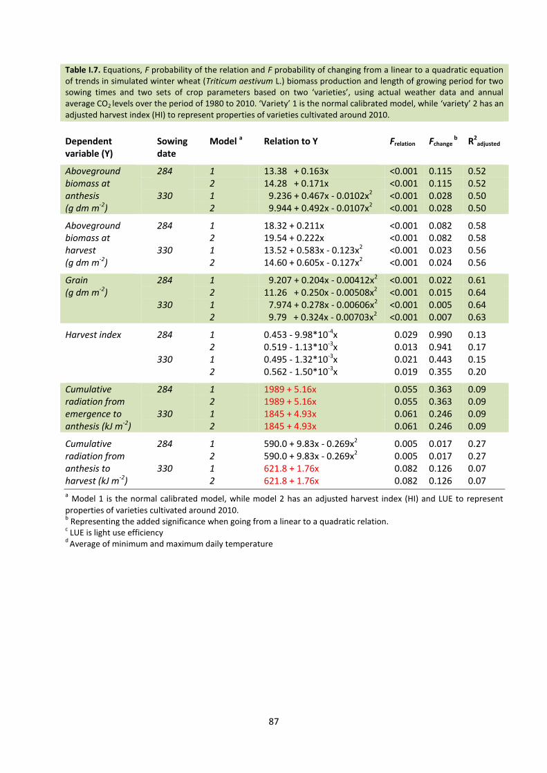
87

Table I.7. Equations, F probability of the relation and F probability of changing from a linear to a quadratic equation of trends in simulated winter wheat (Triticum aestivum L.) biomass production and length of growing period for two sowing times and two sets of crop parameters based on two ‘varieties’, using actual weather data and annual average CO2

levels over the period of 1980 to 2010. ‘Variety’ 1 is the normal calibrated model, while ‘variety’ 2 has an

adjusted harvest index (HI) to represent properties of varieties cultivated around 2010.

Dependent variable (Y)

Sowing date

Model a Relation to Y Frelation Fchange b R2

adjusted

Aboveground biomass at anthesis (g dm m-2)

284 1 13.38 + 0.163x <0.001 0.115 0.52 2 14.28 + 0.171x <0.001 0.115 0.52 330 1 9.236 + 0.467x - 0.0102x2 <0.001 0.028 0.50 2 9.944 + 0.492x - 0.0107x2 <0.001 0.028 0.50

Aboveground biomass at harvest (g dm m-2)

284 1 18.32 + 0.211x <0.001 0.082 0.58 2 19.54 + 0.222x <0.001 0.082 0.58 330 1 13.52 + 0.583x - 0.123x2 <0.001 0.023 0.56 2 14.60 + 0.605x - 0.127x2 <0.001 0.024 0.56

Grain (g dm m-2)

284 1 9.207 + 0.204x - 0.00412x2 <0.001 0.022 0.61 2 11.26 + 0.250x - 0.00508x2 <0.001 0.015 0.64 330 1 7.974 + 0.278x - 0.00606x2 <0.001 0.005 0.64 2 9.79 + 0.324x - 0.00703x2 <0.001 0.007 0.63

Harvest index 284 1 0.453 - 9.98*10-4x 0.029 0.990 0.13

2 0.519 - 1.13*10-3x 0.013 0.941 0.17 330 1 0.495 - 1.32*10-3x 0.021 0.443 0.15 2 0.562 - 1.50*10-3x 0.019 0.355 0.20

Cumulative radiation from emergence to anthesis (kJ m-2)

284 1 1989 + 5.16x 0.055 0.363 0.09 2 1989 + 5.16x 0.055 0.363 0.09 330 1 1845 + 4.93x 0.061 0.246 0.09 2 1845 + 4.93x 0.061 0.246 0.09

Cumulative radiation from anthesis to harvest (kJ m-2)

284 1 590.0 + 9.83x - 0.269x2 0.005 0.017 0.27 2 590.0 + 9.83x - 0.269x2 0.005 0.017 0.27 330 1 621.8 + 1.76x 0.082 0.126 0.07 2 621.8 + 1.76x 0.082 0.126 0.07

a Model 1 is the normal calibrated model, while model 2 has an adjusted harvest index (HI) and LUE to represent

properties of varieties cultivated around 2010. b Representing the added significance when going from a linear to a quadratic relation.

c LUE is light use efficiency

d Average of minimum and maximum daily temperature

88

Appendix II

Table II.1 Observed development stages of winter wheat (Triticum aestivum L.) sown from September to January in five different years.

Year Sowing date Emergence

(F1)* Start grain filling

(F10.5.4) Maturity

(F11.3)

1979

21-9-1978 30-9-1978 5-7-1979 12-8-1979

1979 16-10-1978 31-10-1978 11-7-1979 20-8-1979

1979 15-11-1978 22-12-1978 11-7-1979 29-8-1979

1979 15-12-1978 3-4-1979 26-7-1979 5-9-1979

1980 17-10-1979 8-11-1979 26-6-1980 12-8-1980

1980 1-11-1979 29-11-1979 28-6-1980 13-8-1980

1980 15-11-1979 8-12-1979 30-6-1980 15-8-1980

1980 17-12-1979 25-2-1980 7-7-1980 16-8-1980

1982 16-10-1981 2-11-1981 1-7-1982 4-8-1982

1982 4-11-1981 30-11-1981 1-7-1982 5-8-1982

1982 18-11-1981 29-12-1981 4-7-1982 6-8-1982

1982 22-1-1982 12-3-1982 8-7-1982 8-8-1982

1983 15-10-1982 26-10-1982 29-6-1983 30-7-1983

1983 1-11-1982 19-11-1982 4-7-1983 1-8-1983

1983 15-11-1982 18-12-1982 6-7-1983 3-8-1983

1983 16-12-1982 19-1-1983 8-7-1983 6-8-1983

1983 17-1-1983 7-3-1983 12-7-1983 9-8-1983

1984 14-10-1983 31-10-1983 6-7-1984 18-8-1984

1984 1-11-1983 25-11-1983 11-7-1984 20-8-1984

1984 16-11-1983 26-12-1983 16-7-1984 23-8-1984

1984 20-12-1983 16-1-1984 18-7-1984 25-8-1984

1984 16-1-1984 14-3-1984 25-7-1984 29-8-1984

* Development stage according to Feekes scale of cereal development.

89

Appendix III Table III.1 Observed yields of different winter wheat (Triticum aestivum L.) varieties sown at different locations and sowing densities in the Netherlands from 1976 to 1998.

Source

Location

Sowing date

Sowing densitya

(seeds m-2)

Plant densityb

(plants m-2)

Initial weight leaves (g m-2)

Initial weight stem (g m-2)

Aboveground biomass (kg ha-1)

Grain yield (kg ha-1)

Variety

(Darwinkel, 1994) Ebelsheerd 24-10-1990 375 290 0.10 0.06 1,581 751 Herzog, Obelisk and Urbanc

(Darwinkel, 1994) Westmaas 26-10-1990 325 168 0.06 0.03 1,726 832 Herzog, Obelisk and Urban

(Darwinkel, 1994) Wijnandsrande 26-10-1990 300 178 0.06 0.03 1,496 723 Herzog, Obelisk and Urban

(Darwinkel, 1985) PAGVd 19-10-1976 413 280 0.10 0.05

705.5 Caribo

(Darwinkel, 1985) PAGV 22-9-1978 425 319 0.11 0.06

774.4 Caribo (Darwinkel, 1985)

PAGV 6-10-1978 425 319 0.11 0.06

694.5 Caribo (Darwinkel, 1985)

PAGV 24-10-1978 425 319 0.11 0.06

612.9 Caribo (Darwinkel, 1985)

Bemmelenhoeve 3-10-1978 350 263 0.09 0.05

791.4 Donata (Darwinkel, 1985)

Bemmelenhoeve 30-10-1978 350 263 0.09 0.05

781.2 Donata (Darwinkel, 1985)

PAGV 20-9-1979 338 170 0.06 0.03

822.0 Arminda (Darwinkel, 1985)

PAGV 22-10-1979 338 200 0.07 0.04

761.6 Arminda (Darwinkel, 1985)

Westmaas 20-9-1979 500 310 0.11 0.06

827.1 Okapi (Darwinkel, 1985)

Westmaas 17-10-1979 500 310 0.11 0.06

824.5 Okapi (Darwinkel, 1985)

PAGV 14-10-1980 150 135 0.05 0.03

772.7 Arminda (Darwinkel, 1985)

PAGV 15-10-1980 300 270 0.10 0.05

775.2 Arminda

90

(Darwinkel, 1985) PAGV 16-10-1980 450 390 0.14 0.08

742.1 Arminda

(Darwinkel, 1985) PAGV 17-10-1980 600 520 0.19 0.10

763.3 Arminda

(Darwinkel, 1985) Feddemaheerd 17-9-1980 625 469 0.17 0.09

907.0 Okapi

(Darwinkel, 1985) Feddemaheerd 13-10-1980 625 469 0.17 0.09

774.4 Okapi

(Darwinkel, 1985) Bemmelenhoeve 1-10-1980 620 465 0.17 0.09

901.0 Okapi

(Darwinkel, 1985) Westmaas 25-9-1980 625 480 0.17 0.09

871.3 Arminda

(Darwinkel, 1985) Westmaas 22-10-1980 625 480 0.17 0.09

832.2 Arminda

(Darwinkel, 1985) Rusthoeve 7-11-1980 375 306 0.11 0.06

790.5 Arminda

(Darwinkel, 1985) Rusthoeve 7-11-1980 625 527 0.19 0.10

796.5 Arminda PPO praktijkonderzoek PAV PPOd 17-10-1996 350 260 0.09 0.05 1,207.7

Vivant

PPO praktijkonderzoek PAV PPO 17-10-1996 350 260 0.09 0.05 1,973.3 1015.6 Vivant PPO praktijkonderzoek PAV PPO 11-1-1999 400 260 0.09 0.05 1,039.7

Ritmo

PPO praktijkonderzoek PAV PPO 11-1-1999 400 260 0.09 0.05 1,962.9 963.5 Ritmo PPO praktijkonderzoek PAV PPO 6-10-1998 350 260 0.09 0.05 1,305.5

Ritmo

PPO praktijkonderzoek PAV PPO 6-10-1998 350 260 0.09 0.05 2,238.3 1115.3 Ritmo

a Red numbers are estimated based on seed weight per m

-2.

b Green numbers are estimated based on the sowing density.

c Average of three varieties.

d PAGV has become PAV PPO.

91