Munich Personal RePEc Archive

The Impact of Central Bank’sintervention in the foreign exchangemarket on the Exchange Rate: The caseof Zambia (1995-2008)

Mwansa, Katwamba

London Metropolitan University

May 2009

Online at https://mpra.ub.uni-muenchen.de/22428/

MPRA Paper No. 22428, posted 04 May 2010 05:58 UTC

1

THE IMPACT OF CENTRAL BANK’S INTERVENTION IN

THE FOREIGN EXCHANGE MARKET ON THE EXCHANGE RATE: THE CASE OF ZAMBIA

(1995-2008)

KATWAMBA MWANSA -07061022

DISSERTATION SUBMITTED IN PARTIAL FULFILMENT OF THE REQUIREMENTS OF

LONDON METROPOLITAN BUSINESS SCHOOL

LONDON METROPOLITAN UNIVERSITY FOR THE DEGREE OF

MASTERS OF SCIENCE IN INTERNATIONAL

ECONOMICS

MAY 2009

2

DEDICATION

TO MY WIFE AND CHILDREN

3

TABLE OF CONTENTS

Acknowledgements

Abstract

List of tables

List of figures

CHAPTER 1: INTRODUCTION

1.1 Introduction.............................................................10

1.2 Objectives and aims of the study....................................17

1.3 Outline of the study....................................................17

CHAPTER 2: REVIEW OF LITERATURE

2.1 Introduction..............................................................19

2.2 Theoretical Review......................................................19

2.3 Empirical Literature.....................................................35

CHAPTER 3: EXCHANGE RATE POLICY IN ZAMBIA.

3.1 Background...............................................................45

3.2 An account of foreign exchange regimes ............................47

3.3 Parallel foreign exchange black market..............................50

CHAPTER 4: DATA AND METHODOLOGY.

4.1 Data description..........................................................52

4.2 Methodology ............................................................56

4.3 The effects of BOZ‟s intervention.....................................57

4.4 Prior Expectations.......................................................60

CHAPTER 5: EMPIRICAL RESULTS

5.1 Conditional Mean........................................................65

5.2 Conditional Variance...............................................67

CHAPTER 6: CONCLUSION

6.0. Conclusion................................................................69

BIBLIOGRAPHY..............................................................71

APPENDIX...................................................................76

4

ACKNOWLEDGEMENTS

Firstly, I wish to thank the God Almighty for His faithfulness during my postgraduate training in

general and specifically during the course of this dissertation. The whole process was miracle

packed.

Secondly, my very special thanks to Professor Nick Sarantis, my supervisor, for the valuable

support and for guidance from topic selection up to completion of the dissertation. He was

extremely patient with me and availed himself for consultation each time I requested for it. I

owe so much to him.

I would like to thank Dr. Nishaal Gootoochum, the module leader, who timely took us through

dissertation writing and made himself available for short notice consultations.

I am also highly indebted to the senior management of the Communications Authority (CAZ); in

particular to the former Chief Executive Officer, Mr. Shuller Habeenzu, the Deputy Chief

Executive Officer Mr. Richard Mwanza and my immediate superordinate Mrs. Susan Mulikita for

endorsing and supporting my sponsorship for this training.

My great thanks and appreciation to my lovely and dearest wife Rachel Mwansa, my daughter

Kalumbu and son Kalinda. They always challenge me to work hard and be an achiever.

Throughout the course of this work they remained supportive, understanding, loving and

encouraging despite the fact I spent less and less time with them. They have always been the

reason why I have pushed my boundaries and succeeded in everything my hands have set to do.

Special thank to Dr.Jonathan Chipili Mpundu, who mentored me from the very beginning of my

studies. He never got tired of guiding me through the various steps of the dissertation until the

very end.

Lastly but certainly not the least I would like to acknowledge the support of my father and

mother, brothers, sisters and friends.

5

ABSTRACT

The central bank of Zambia called Bank of Zambia (BOZ) has, like many other central banks in

both developing and developed economies, been from time to time intervening in the foreign

exchange market by either purchasing or selling foreign exchange (mainly United States of

America Dollars) to the market. Central banks have given a myriad of reasons for this particular

behaviour. Chief among these and which is the focus of this paper is to smooth volatility or

reverse a trend of the domestic currency in this case the kwacha. Despite central banks‟

intervention activities in the foreign exchange markets, literature on the efficacy of these

interventions in terms of impacting domestic currencies has remained controversial. While some

strands of literature seem to suggest that such intervention has an impact on the currencies

some literature disagrees.

Early studies done in the 1980s suggest that intervention operations do not affect the exchange

rate and if they do this effect is very small and only in the short run. More recent studies

however, have found evidence of the effect on both the level and volatility of exchange rates.

Further, recent studies focused on emerging market and developing countries have found strong

evidence of the effect of central banks‟ intervention operations in the foreign exchange market

on exchange rates.

This paper therefore examines the effect of the BOZ‟s foreign currency market interventions on

the level and volatility of the kwacha/ USD exchange rate between 1995 and 2008. In order to

study the impact of interventions on the kwacha, the paper uses monthly data (both sales and

purchases) on foreign exchange intervention and employs the GARCH (1, 1) and Exponential

GARCH frameworks to model volatility. The results from GARCH model suggest that sales of

foreign exchange in this case the $ causes the exchange rate to appreciate while purchases of

the $ cause the exchange rate to depreciate. As for the impact on volatility, the GARCH (1, 1)

model reveals that BOZ interventions increase volatility.

6

Empirical results from the EGARCH model on the other hand suggest that both sales and

purchases of $ cause the exchange rate to appreciate. The results on the impact of intervention

on volatility are mixed though generally intervention appears to be increasing volatility.

7

LIST OF ABBREVIATIONS

BOZ =Bank of Zambia (Zambia‟s central bank)

K = Kwacha (Official exchange rate in Zambia)

$ = United States of America dollar

Fed = Federal Reserve Bank

Y = Japanese Yen

M = Germany Deutschmark

8

LIST OF TABLES

1. Most traded currencies.

2. ADF results for the exchange rate – Level

3. ADF results for the exchange rate – first difference

4. ARCH effects Test.

5. GARCH estimation results.

6. EGARCH estimation results

9

LIST OF FIGURES

1. Foreign Exchange Turnover

2. GDP Growth in Zambia (1995-2008)

3. Zambia‟s current account position( 1995-2008)

4. BOZ sales of USD IN 000 (1995-2008)

5. BOZ purchases of USD IN 000 (1995-2008)

6. Monthly kwacha and USD exchange rate (1995-2008)

7. GARCH conditional variance

8. EGARCH condition variance

9. EGARCH LS residual

10

1 INTRODUCTION

Foreign exchange intervention is the process by which central banks and other monetary

authorities either buy or sell foreign exchange in the foreign exchange market normally

against their own currencies in line with some policy objective. Some of the objectives

include among others to control inflation or maintain internal balance; to maintain external

balance and prevent resource misallocation or preserve competitiveness and boost growth;

and to prevent or deal with disorderly markets or crises. To achieve these objectives, central

banks might seek to target the level of the exchange rate, dampen exchange rate volatility

or influence the amount of foreign reserves.

There are a number of reasons why central banks intervene in the foreign exchange markets.

There are however, four common reasons; to calm disorderly markets (smoothing volatility),

cure exchange rate misalignment, signal future monetary policy and build international

reserves.

Exchange rates like many other financial assets exhibit volatility trends which may result in

loss of liquidity. This volatility may also have adverse effects on international trade, the

external balance and threaten the orderly functioning of the market. Central banks may

therefore intervene to calm this disorderly behaviour.

There are times that exchange rates drift away from fundamentals and what monetary

authorities consider to be the equilibrium level. Therefore, central banks may be forced to

try and reverse this misalignment and bring the exchange rate back to its normal path.

Moreno (2005) reporting on a survey of why central banks in emerging market economies

intervened revealed that policymakers are typically concerned not just with how much the

exchange rate might deviate from equilibrium but with how quickly it does so. Intervention

will often attempt to slow the rate of change in the exchange rate without preventing trend

11

changes, a policy that is known as „leaning against the wind”. While intervention of this kind

typically occurs when the exchange rate is moving away from equilibrium, it can sometimes

occur if the exchange rate is moving back to equilibrium, but “too quickly”. Slowing the rate

of change in the exchange rate can stop herding behaviour by acting as a circuit breaker. By

reducing uncertainty, this type of intervention may facilitate foreign exchange market

development. On the other hand, by acting as a provider of “insurance” against rapid

exchange rate movements, official intervention could also undermine incentives for the

development of hedging capability in the private sector. Chile, Israel and Mexico were given

as examples.

Intervention may also be used to signal future changes to monetary policy and calm

expectations if monetary policy is changed unexpectedly which might otherwise lead to a

loss in confidence and thereby induce an unwarranted moves in the exchange rate.

Finally, central banks may want to build international reserves of foreign currencies and so

they will enter the foreign exchange market to purchase a foreign currency. International

reserves are sometimes used as collateral to attract foreign investors.

The practice of intervention has been around for a while though it really intensified after the

collapse of the Bretton Woods System in 1972. Before then intervention was allowed for the

sake of keeping exchanges rates within agreed parity bands. However, after the demise of

the fixed exchange rate system, the discretion to intervene in the foreign exchange market

became incumbent upon individual states and their monetary authorities. To this extent the

International Monetary Fund (IMF) even issued guidelines on how member states should

conduct their intervention activities. Historically, the G -5 countries who included Japan,

Germany, the United States of America, and France signed the Plaza Agreement in 1995. The

agreement was about coordinated intervention. Consequently, over the years all major

developed countries have intervened in the foreign exchange market on a number of

12

occasions albeit the frequency now is very minimal. However, developing countries are now

more active in this area.

Canales-Krijenko (2003) in a survey of central banks‟ foreign exchange market intervention

revealed that central banks issuing major currencies were seldom active in the foreign

exchange market because they had developed policy frameworks that target short-term

interest rates and exchange rate policies that limited foreign exchange intervention to calm

disorderly market conditions. On the other hand most central banks in developing and

transitional economies were more active in the foreign exchange market across all exchange

rate regimes.

However, the key question in academia, politics and government is whether this intervention

is really effective. Unfortunately, this question and the debate around it has been raging

from the time of the introduction of the floating exchange system in the early 1970s, and it

does not seem to be receding. There are three different views points on this matter.

One strand of thought posits that intervention operations do not at all affect the level or

volatility of the exchange. Another school of thought states that intervention while not being

only ineffectual at influencing the level of the exchange rate also increases the volatility of

the exchange. The last strand of thought states that intervention operations do influence the

exchange rate and do also calm disorderly markets in the process arresting volatility

(Dominguez 1998, Edison et al 2003)

Empirical studies conducted in the early 1980s have suggested that intervention whether

sterilized or not was ineffective in as far as affecting the exchange rate was concerned. Of

particular note was the Jurgensen Report of 1983 which categorically stated that

intervention was in the main ineffective. However, studies into the phenomenon conducted

after the 1990s using high –frequency central bank intervention data which was missing in the

1980s studies suggest that intervention does have an effect after all. It should also be noted

that despite the scepticism about the efficacy of intervention both in academia and public

13

policy sectors, it is ironical that most central banks both in developing and developed

countries continue to intervene in their foreign exchange markets. This should therefore

point to the fact that central banks believe intervention does work and is effective in

achieving their policy objectives.

Broadly speaking an exchange rate is the price of one currency in relation to another. This

price is either expressed in domestic currency units per unit of foreign currency or as foreign

currency units per unit of the domestic currency (Pilbeam 2006). In this paper the former

definition is adopted such that we express the exchange rate as kwacha units per United

States of America dollar unit. When we talk about exchange rates we are invariably talking

referring to the nominal exchange rate. The definition of nominal exchange rate is alluded to

earlier. In contrast, a real exchange rate is the price of domestic goods to relative to foreign

goods or the number of foreign goods one gets in exchange for domestic goods.

The foreign exchange market is where currency trading takes place. It is where institutions

facilitate the buying and selling of foreign currencies. It involves a process where one party

purchases a quantity of one currency in exchange for paying a quantity of another. Currently,

foreign exchange markets are the most liquid financial markets in the world.

The BIS (2007) reported that turnover in the traditional foreign exchange markets had grown

unprecedented by 69 per cent since April 200 4 to $3.2 trillion (See graph below).

The U.S. dollar which is the international reserve currency continues, as Table 1 depicts, to

be the most traded currency world over.

14

Figure 1: Foreign exchange Turnover (USD millions)

TABLE 1: MOST TRADED CURRENCIES (2007)

Source: BIS

Rank Currency ISO 4217 code

(Symbol) % daily share (April 2007)

1  United States dollar USD ($) 86.3%

2  Euro EUR (€) 37.0%

3  Japanese yen JPY (¥) 17.0%

4  Pound sterling GBP (£) 15.0%

5  Swiss franc CHF (Fr) 6.8%

6  Australian dollar AUD ($) 6.7%

7  Canadian dollar CAD ($) 4.2%

8-9  Swedish krona SEK (kr) 2.8%

8-9  Hong Kong dollar HKD ($) 2.8%

10  Norwegian krone NOK (kr) 2.2%

11  New Zealand dollar NZD ($) 1.9%

12  Mexican peso MXN ($) 1.3%

13  Singapore dollar SGD ($) 1.2%

14  South Korean won KRW (₩) 1.1%

Other 14.5%

Total 200%

15

There are a number of participants in the foreign exchange market who include the following:

The central banks or monetary authorities. These play an important role in the foreign

exchange market. They attempt to control the money supply, inflation and or interest rates

and often have official or unofficial target rates for their currencies. They frequently

intervene to buy and sell their currencies in a bid to influence the rate at which their

currency is traded.

Commercial banks. The interbank market caters for both the majority of commercial

turnover and large amounts of speculative trading. Some trading is undertaken on behalf of

customers but much is conducted by proprietary desks trading for the bank‟s own account.

Commercial companies. They include international investors, multinational corporations

who need foreign exchange for the purposes of running their businesses. Normally, they do

not directly purchase or sell foreign exchange themselves but they place buy/sell orders with

commercial banks. Though their impact on exchange rates is minimal, commercial companies‟

trade flows are an important factor in the long term direction of a currency‟s exchange rate.

Some firms can have an unpredictable impact when very large positions are covered due to

exposures that are not widely known by other market participants.

Foreign exchange brokers. Often banks do not trade directly with one another, but they

transact through foreign exchange brokers.

Money transfer/ Remittance companies. These perform high volume low value transfers

generally by economic migrants to their home country. One example of such institutions is

Western Union.

Hedge funds act as speculators. A majority of foreign exchange transactions are

speculative. Economic agents that buy and sell foreign exchange have no plan to actually

16

take delivery of the currency in the end rather they were solely speculating on the

movement of that particular currency. They may control billions of equity and may borrow

billions more and thus overwhelm intervention by central banks to support almost any

currency if the economic fundamentals are in the hedge funds favour.

Foreign exchange markets in emerging markets and developing economies like Zambia are

fundamentally different from those of developed countries. They are small in size,

undercapitalized and underdeveloped, sometimes highly regulated by the central banks and

other monetary authorities.

Disyatatat and Galati (2005) describe the situation in emerging market economies as

follows: (i) the size of intervention relative to market turnover tends to be larger, (ii) the

existence of some form of capital controls limiting access to international capital markets

gives central banks in these countries greater leverage in the market, and (iii) the lower

level of sophistication of the domestic market along with stringent reporting requirements

may endow central banks with a greater informational advantage not only with respect to

fundamentals but also aggregate order flows and net open positions of major traders.

The size of foreign exchange intervention relative to the turnover in the foreign exchange

market has a telling effect on the impact of intervention on the exchange rate. Foreign

exchange intervention in developing countries accounts for a much larger proportion of total

foreign exchange market turnover than in developed countries.

Through the existence of foreign exchange controls, like surrender requirements to the

central banks, some developing countries increase the size of intervention in comparison to

the size of the foreign exchange market.

17

Central banks in developing countries also possess an information advantage over economic

agents which their counterpart institutions in developed economies do not possess. For

example some of them might have a better grasp of aggregate foreign exchange order flow

including future monetary and exchange rate policy than economic agents.

When examining the efficacy of intervention therefore this clear distinction on the

environments in emerging market economies as opposed to developed ones is very essential.

The factors highlighted above seem to make central bank intervention in developing and

transitional economies more effective than in developed ones.

This is supported by a number of studies (Edison et al 2003) (Disyatat and Galati 2005)

(Simatele 2004) (Domac and Mendoza 2004) (Kim et al 2000).

This paper studies the impact of the central of Bank, the Bank of Zambia‟s (BOZ)

intervention in the foreign exchange market in Zambia on the domestic currency, the kwacha

(K). It does not distinguish between sterilized or unsterilised intervention due to the limited

time span of the research. Therefore, it focuses on the fact the BoZ intervened in the foreign

exchange market. The BOZ has been intervening in the foreign exchange market ever since

the start of the flexible exchange rate system in 1992. However, due to data unavailability

the period 1992 -1994 has been excluded from the sample period.

2) Aims and Objectives

This paper intends to establish whether the Bank of Zambia‟s intervention in the foreign

exchange market from 1998 to 2008 has had an impact on the level and volatility of the

kwacha.

3) Outline of the Study

The study is divided into a further five chapters. Chapter two provides the review of both

theoretical and empirical literature. It outlines the assumptions, predictions, and weaknesses

18

of various exchange rate determination models and channels through which central bank

intervention in the foreign exchange market affects exchange rates. Chapter three provides a

brief overview of Zambia and the exchange rate policy history in the country from

independence to date. Chapter four describes the data used in the study namely sales and

purchases of the United States Dollars (USD). It also highlights the EGARCH and GARCH models

used to model the impact of Bank of Zambia‟s intervention impact on the kwacha. Chapter

five provides the empirical results while chapter six is the conclusion.

19

CHAPTER 2 REVIEW OF LITERATURE

2. 1. THEORETICAL LITERATURE.

Exchange rate determination is often interpreted to arise from three basic models. These are

the purchasing power parity, monetary and portfolio balance models. Additionally in the recent

past the signalling/expectations and microstructure/order flow have been identified as channels

through which foreign exchange market intervention may affect the exchange rate. These five

theories are discussed below:

2.1.1. PURCHASING POWER PARITY (PPP) MODEL

This is the oldest and widely used model for assessing long run exchange rate movements. It

states that changes in exchange rates between currencies will tend to reflect changes in relative

countries‟ price levels.

Its basic tenet according to Pilbeam (2006) is the law of one price which posits that once prices

are converted into one currency, the same good should sell for the same price in a another

country.

ASSUMPTIONS

The model assumes the following:

The goods are tradable.

The goods are homogenous.

There are no impediments to trade such as tariffs, transport and transaction costs.

The price systems works.

The economies are operating at full employment.

There is full information across economies.

There are two versions of the model. The absolute PPP is based on the strict interpretation of

the law of one price while the relative one is a more relaxed and weaker version.

20

The absolute version postulates that the equilibrium exchange rate between two countries‟

currencies is determined entirely by the ratio of the two countries‟ national price levels as

follows:

S= P ........................................................ 2.0

P*

Where S is the domestic exchange rate, P and P* represent domestic and foreign consumer price

indices respectively.

Equation 2 states that if the foreign prices go up relative to domestic ones, then the domestic

currency will appreciate in value. Conversely, if the prices of domestic goods increase relative

to the foreign ones, then the domestic currency will depreciate.

The relative version overcomes some hurdles of its predecessor by recognizing the presence of

transport costs and tariffs in international trade. It posits that the exchange rate will be

determined by inflation differential between two countries.

%ΔS =%ΔP - %ΔP*....................................... 2.1.

Where %ΔS is the percentage change in the exchange rate,

%ΔP in the domestic inflation and

%ΔP* change in the foreign inflation.

The relative PPP version predicts that if relative prices double in the home country between a

base period and some subsequent date, the exchange rate will depreciate by an equal

proportion.

21

WEAKNESSES

The model has performed badly in determining exchange rates especially after the introduction

of flexible exchange rate regimes due to a number of flaws. Firstly, it is difficult to tell whether

or not the model applies to both tradable and non-tradable sectors. If there is a difference

between price inflation in the traded and non-traded sectors across countries then the model

will not capture these effects. Secondly, countries have different weights attached to a similar

set of goods and services. This will therefore lead to greater disparity from aggregate PPP.

Further, assumptions related to international movement of goods are not realist because in

reality transaction and transport costs will always exist when goods move from one country to

the other. Finally empirically the model has performed very badly.

22

2.1 2.MONETARY MODELS

The monetary models posit that the exchange rate should be viewed as an asset price which

depends on the current and expected future values of relative supply of domestic and foreign

financial assets. They seek to explain how changes in the domestic and foreign supply and

demand for money both directly and indirectly influence the exchange rate.

The paper examines the Flexible –Price and Sticky- Price monetary models.

FLEXIBLE –PRICE MODEL

The Flexible-price Monetary Model is attributed to Frenkel (1976) Mussa (1976) and Bilson (1978).

Though being a monetary (asset) model it is an extension of the PPP model.

Hallwood and MacDonald (2008) state that the model depends on PPP equation in order to

explain the exchange rate.

ASSUMPTIONS

Domestic and foreign bonds are perfect substitutes and therefore the Uncovered Interest

Parity (UIP) condition holds continuously(S=P-P*)

Prices and wages are all flexible both downwards and upwards.

There is perfect capital mobility.

Absolute PPP holds continuously.

Demand to hold real money balances is positively related to real income and negatively

related to the domestic interest rate.

Money supply and real income are exogenously determined.

The money market is the only important asset market.

23

From the above assumptions, we can derive the main equation (reduced form) of the model

which is:

S= (M- M*) – k(y- y*) +θ(r- r*)............................... (2.2)

s = nominal spot exchange rate (domestic currency price of foreign currency)

m = domestic money supply

y = domestic scale variable (usually income level)

r = opportunity cost of holding money usually interest rate,

θ = constant

(Corresponding foreign magnitudes are denoted by an asterisk)

PREDICTIONS

The predictions of the flexible-price monetary model are as follows:-

Firstly there is proportionality between relative monies and the exchange rate so that the

coefficient on the money supply m is expected to be 1. In other words, an increase in domestic

money supply relative to foreign stock would lead to a rise in the exchange rate i.e.

depreciation of the domestic currency in terms of the foreign currency.

A rise in domestic real income, ceteris paribus, creates an excess demand for domestic money

stock. In an attempt to increase their real money balance, domestic residents reduce

expenditure and prices fall until money market equilibrium is achieved. Through PPP, falling

domestic prices (with foreign prices constant) imply an appreciation of the domestic currency in

terms of the foreign currency. (Sarno and Taylor 2008)

Finally, an increase in domestic interest rates leads to a depreciation of domestic currency.

WEAKNESSES

The major weakness of the model is its reliance on the PPP model and its assumptions are also

oversimplified.

24

THE STICKY-PRICE MODEL

The Dornbusch Sticky-Price Model has the same features as the Flexible –Price model in the long

run but differs in the short run. In this horizon it is assumed that prices and wages are not

adjustable downwards because they are „sticky‟. This means that the goods market does not

continuously clear in the short-run and that the PPP condition does not hold but it does so in the

long-run.

ASSUMPTIONS

Goods prices and wages tend to change slowly downward in the short run.

Uncovered interest parity (UIP) holds continuously.

There are jump variables in exchange rates which compensate for stickiness of goods prices.

There is money-neutrality.

SHORT RUN OVERSHOOTING

Due to price stickiness goods prices do not continuously clear. So there is an asymmetry of

adjustment between goods and assets markets. The Sticky –Price Pilbeam (2006)

model is given below

Es = Θ (Ŝ – S) Θ > 0. (2.3)

Where Ŝ is the exchange rate‟s long run value while S is the spot rate and Θ is the adjustment

parameter and the gap between the current exchange rate S and its long-run equilibrium value Ŝ.

There is “overshooting” of the exchange in the short –run when there is an unexpected increase

in domestic money supply, the exchange rate and prices level are expected to change

appropriately. However, due to price stickiness this does not happen. This does not hence clear

the money market but instead it is cleared by a fall in interest rate.

25

As a result international investors anticipate a depreciation of the currency to compensate for

the lower interest rates. The domestic currency then appreciates to a level which exceeds

(overshoots) its long-run value. This follows from the UIP which implies that the domestic

interest rate can only be below the foreign rate if economic agents expect the exchange rate to

appreciate which can only happen if the current spot rate moves more than the long run value.

In essence the extent of the overshooting incidences hinges on the interest rate semi-elasticity

of the demand for money.

LONG RUN EQUILIBRIUM

In the long run the PPP equation (S= P-P*) holds. After the currency overshoots its long run value

in the short run, it will eventually start depreciating as prices adjust until its long run PPP is

satisfied.

PREDICTIONS

According to equation 2.3 the expected rate of depreciation of a currency is determined by the

speed of the adjustment parameter and the gap between the current exchange rate and its long

run value. If S is above Ŝ then it is anticipated that the local currency will appreciate.

Conversely if the spot rate is below its long run value, the currency will be expected to

depreciate.

In the long run the exchange rate will be determined by relative prices of goods between

countries.

WEAKNESSES

The major weakness of this model like other asset theories is that there is no role for the

current account in determining the exchange rate when in real life since exchange rates have an

impact on the current account.

The other problem is that this model omits a range of assets and only considers money.

26

THE PORTFOLIO BALANCE MODEL (PBM)

The PBM is a dynamic exchange rate determination model which is hinged upon the interplay of

asset markets, current account balance, prices and the rate of asset accumulation. It introduces

the current account aspect which monetary models did not capture. The current account plays a

prominent role in the exchange rate determination while the exchange rate affects the trade

balance and current account and hence the net foreign assets.

Here the central role of wealth variables is recognized; economic agents allocate their wealth

among different assets, and the proportion of each asset held depends on the risk and return

assessments economic agents make.

ASSUMPTIONS

Three assets are held by economic agents and authorities. These are domestic monetary

base (M), domestic bonds denominated in the domestic currency (B) and foreign bonds

denominated in foreign currency (F).

Domestic and foreign assets are imperfect substitutes. Therefore uncovered interest

parity does not hold.

Domestic prices and output are fixed following a policy disturbance.

The country concerned is too small to influence world exchange rates.

Money demand depends not only on income but also on wealth and interest rates.

Net exports are a positive function of the real exchange rate.

27

SHORT RUN EQUILIBRIUM

The total wealth (W) of economic agents consists of the domestic monetary base (M), domestic

bonds (B) and foreign bonds as follows (F);

W= M + B+ F........................................... (2.4)

The short run equilibrium is given by:

B*= T( S/P) + i* B* T› 0 ........(2.5)

Where B* capital account

i* B* is the net debt service receipts.

The short run equation (2.5) shows the rate of change of the capital account as equal to the

current account which is also in turn equal to the sum of the trade balance and net debt service

receipts. This means that the trade balance depends positively on the level of the real

exchange rate.

When domestic interest rates rise, economic agents adjust their portfolio by substituting

domestic for foreign bonds. This causes the demand for foreign assets to decline and the money

realised from selling foreign assets is converted into the domestic currency which results into

the fall of the spot rate.

28

LONG RUN EQUILIBRIUM

In the long run, it is the interplay between the real sector and the financial markets that lead

the economy to its long run status. Equilibrium in the long run takes place when the domestic

price level and the quantity of foreign bonds are such that there is a zero balance on the current

account. At this point there is no accumulation or de-cummulation of wealth. When the current

account is in balance the rate of change in the exchange rate will be zero.

CA= T(S/P) + i* B*

Where T (.) is a function of competitiveness............... (2.6)

A current account surplus (deficit) is associated with a domestic currency appreciation

(depreciation) which tends to eliminate the surplus (deficit). This means that in the long run

exchange rate determination is a macroeconomic problem involving the interaction of goods and

asset markets.

PREDICTIONS

The model predicts that certain monetary authority policy actions have short-run effects on the

exchange rate.

Firstly, when monetary authorities embark on expansionary foreign exchange operations by

buying foreign bonds from the private sector, this will increase the sector‟s holdings of money

but a downfall of foreign bonds. This will lead Copeland (2008) to a downward adjustment of

interest rates and a rise in the price of foreign currency and therefore currency

depreciation.

Expansionary open market operations which increase the private sectors holdings of money and

reduction of domestic bonds will lead to domestic currency depreciation and a fall in domestic

interest rates.

29

The difference between this and the first is qualitative rather than quantitative Copeland (2008))

Monetary authorities can also embark an expansionary foreign exchange activity but accompany

this with contractionary open market operations by first purchasing foreign assets with domestic

money base and the offset the increase in the money supply by selling domestic bonds (sterilized

foreign exchange intervention). The short run effect of this policy measure is that it will

increase the supply of domestic bonds but decrease the private sector‟s levels of foreign assets.

The result is a depreciation of the exchange rate and a rise in interest rates.

30

CHANNELS OF INTERVENTION.

2.1.4 PORTFOLIO BALANCE CHANNEL

In line with the portfolio balance model discussed, this channel postulates that investors hold

three types of assets in different proportions and because foreign and domestic assets are

imperfect substitutes, central bank intervention which alters the asset supplies relative

outstanding supply of domestic assets will require a change in the expected relative returns.

This will culminate in a change of the exchange rate.

2.1.5 THE SIGNALLING CHANNEL

This channel was developed by Mussa (1981). He started from the general monetarist view of

exchange rates being assets. This asset market view of exchange rates postulated that exchange

rates as relative assets prices like other assets were impacted upon by current events as well as

the market‟s expectation of future events. Therefore, they changed from time to time due to

the receipt of new information that changed the market‟s view of the economically appropriate

exchange rate.

FIVE FEATURES OF EXCHANGE RATES

Mussa identified five key features of the asset market view of exchange rates:

The exchange rate being a relative price of two highly durable currencies means that the

prevailing exchange rate is conceived by the market to be linked to future exchanges rates. The

market knows that the fundamentals determining the prevailing exchange rate will also to a

greater extent affect the future rates.

The central bank can control the supply of currencies in an economy, therefore the central

bank‟s monetary policy is of first order of importance for the behaviour of exchange rates.

31

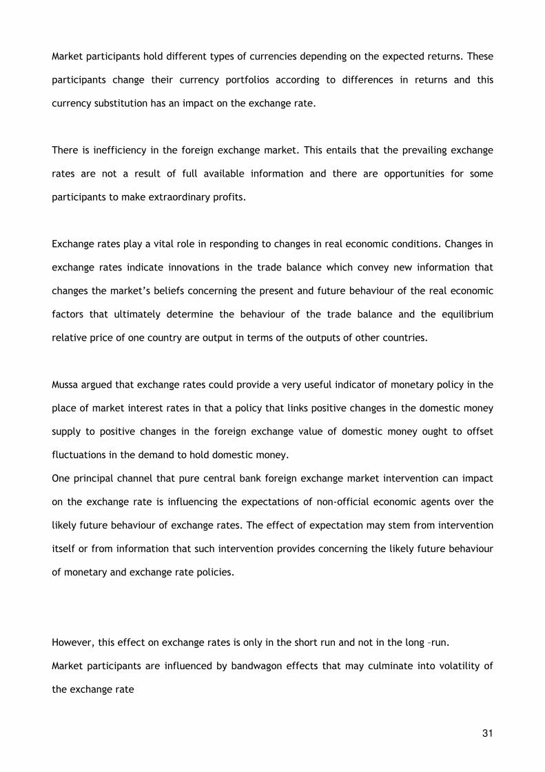
Market participants hold different types of currencies depending on the expected returns. These

participants change their currency portfolios according to differences in returns and this

currency substitution has an impact on the exchange rate.

There is inefficiency in the foreign exchange market. This entails that the prevailing exchange

rates are not a result of full available information and there are opportunities for some

participants to make extraordinary profits.

Exchange rates play a vital role in responding to changes in real economic conditions. Changes in

exchange rates indicate innovations in the trade balance which convey new information that

changes the market‟s beliefs concerning the present and future behaviour of the real economic

factors that ultimately determine the behaviour of the trade balance and the equilibrium

relative price of one country are output in terms of the outputs of other countries.

Mussa argued that exchange rates could provide a very useful indicator of monetary policy in the

place of market interest rates in that a policy that links positive changes in the domestic money

supply to positive changes in the foreign exchange value of domestic money ought to offset

fluctuations in the demand to hold domestic money.

One principal channel that pure central bank foreign exchange market intervention can impact

on the exchange rate is influencing the expectations of non-official economic agents over the

likely future behaviour of exchange rates. The effect of expectation may stem from intervention

itself or from information that such intervention provides concerning the likely future behaviour

of monetary and exchange rate policies.

However, this effect on exchange rates is only in the short run and not in the long –run.

Market participants are influenced by bandwagon effects that may culminate into volatility of

the exchange rate

32

The central bank has control over money supply and has knowledge about its future monetary

policy which market participants do not have. The central bank therefore may intervene in the

foreign exchange market to guide the behaviour of exchange rates in line with its long–run

monetary policy. There is a moral hazard in intervention in that market participants will not

always believe that central bank pronouncements about future policy and will undertake

measures that minimize their risk. Through sterilized intervention, the central bank signals

future monetary policy, the market by observing this intervention expands its information set

and changes its expectations of the existing and future exchange rates. When the participants

revise their expectations of future fundamentals, they also revise their expectations of future

spot exchange rates which in turn changes the existing exchange rate. If the central bank

intervenes by buying the domestic currency, market participants will change their perceptions

about future monetary policy and anticipate a tighter monetary policy in the future. This will

translate consequently in the appreciation of the local currency.

33

2.1.6 THE ORDER FLOW (MICROSTRUCTURE) CHANNEL

The contradiction between the traditional macroeconomic approach to exchange rate

determination and reality obtaining in foreign exchange markets led to a growing interest in the

market microstructure.

According to this model, a more realistic description of the foreign exchange market

microstructure is obtained by relaxing the assumption of identical agents, perfect information or

costless trading and identifying the economic effects of the organisation of foreign exchange

market. The market microstructure might help sort out some of the empirical problems of

conventional models discussed earlier.

In a ground breaking work on this model, Bacchetta and Van Wincoop (2006) were worried about

the poor explanatory power of exchange rate determination theories. They therefore set about

to provide an alternative model which could help resolve the exchange rate puzzle.

ASSUMPTIONS

Market participants are heterogeneous. This comes about in that there are different

investors who differ in terms of information about future macroeconomic fundamentals

and have different exchange rate risk exposure associated with non-asset income.

Some information relevant to exchange rates is not publicly available.

There are differences in the trade mechanisms affected prices.

A small amount of hedge trades can become the dominant source of exchange volatility

when information is heterogeneous while there is no impact when investors have common

information.

34

SHORT RUN

This heterogeneity disconnects the exchange rate from observed fundamentals in the short run.

Secondly, there is a close relationship between the exchange rate and order flow over all time

horizons. Rational confusion plays a vital role in the disconnection process. Investors are not

sure whether the increase in the exchange rate is brought about by an improvement in average

private signals about future fundamentals or an increase in unobserved hedge trades have an

amplified effect on the exchange rate given that they are confused with changes in average

private signals about future fundamentals.

LONG RUN

In the long run rational confusion disappears and investors learn about future fundamentals and

so there is a close link between the exchange rate and the observed fundamentals. The impact

of unobserved hedge trades on the equilibrium price will therefore gradually weaken culminating

to a closer long –run relationship between the exchange rate and observed fundamentals.

ΔP = g(X, I, Z).........................................2.7

Where ΔP is the change in the nominal exchange rate between two transactions.

X is the order flow

I is the inventory cost

Z is the other micro determinants.

According to the above equation (2.7) customers learn about fundamentals from direct sources,

which they use to impact on order flow and then dealers learn about fundamentals from the

behaviour of order flows. Eventually, this affects the trading process and finally the price.

35

2.2 EMPIRICAL REVIEW

Central banks have been intervening in the foreign exchange market ever since the early 1970s.

The practice that initially started with the G-5 countries has now spread all over the world and

while developed countries rarely intervene in their foreign exchange markets, developing and

emerging market economies have pushed up their levers in as far as the practice of intervention

is concerned. The key question that has always been asked is whether this intervention does

intend achieve its objectives of reversing trends or reducing currency volatility. This question

has been empirically tested over the years and therefore there exists a large body of knowledge

on the topic.

The empirical results produced my concerned studies have been mixed. Some studies have

produced evidence that intervention has an impact on both the level and volatility of the

exchange rate while others have found that intervention is actually ineffective.

This chapter provides a critical review of these studies.

One of the very first studies on the effectiveness of central bank intervention on exchange rates

came through a report of a study commissioned by the G7 economic summit at Versailles in 1982.

The Jurgensen Report (1983) concluded that intervention effects were very small and only

occurred in the short-run.

Another study by Bordo and Schwartz (1991) agreed with the Jurgensen Report. They tested the

portfolio balance channel by calculating standard deviations of the daily United States dollar ($)

/ Germany mark (M) as well as the $/ Japanese yen (Y) exchange rates. They found that there

was no evidence that intervention worked and the study concluded that intervention only

increased foreign exchange market uncertainty.

Therefore, the consensus among policy makers and academics during that time was that

intervention was ineffective and if at all it was its effects were only in the short-run.

36

The major problem with these early studies was that the researchers did not use real high

frequency intervention data provided by central banks. During this period central banks were

very secretive in their intervention operations and so they did not release their intervention

data to researchers or indeed the market. So most researchers instead, used proxies of various

kinds as intervention variables. Expectedly therefore their results were not really reliable. Bordo

and Schwart‟s methodology of standard deviation is not a very good econometric model and as

such its estimates are likely to be biased and inefficient.

Sarno and Taylor (2001) reviewed the various channels of intervention and the empirical studies

that had been done in the area of central bank intervention. They opined that due to poor

quality of data in the early studies conducted in the 1980s; most empirical studies indicated that

intervention was ineffective.

On the other hand in the 1990s the veil of secrecy was removed and central banks became more

open and transparent: they released intervention data to the market on a regular and timely

basis. Studies done in this dispensation seem to suggest that central bank intervention is

effective.

A number of studies were undertaken to test the signalling channel hypothesis and most of them

concluded that there was evidence that intervention affected the exchange rate through this

channel.

In this regard, Dominguez (1990) examined 3G central banks‟ foreign exchange interventions

operations. She studied intervention activities of the 3G countries namely the United States of

America (U.S.A), Germany and Japan for the period from 1985 to 1987. Her aim was to establish

whether or not unilateral and coordinated intervention operations influenced market operations.

She used newspaper accounts of intervention to develop an ex-post excess returns model under

the framework of the signalling channel hypothesis. She defined ex-post excess returns as the

realised return that market participants made by borrowing from one institution and lending to

37

another. Intervention was construed to signify conveyance of central bank credible inside

information to the market about future monetary policy. The study found that coordinated

intervention operations consistently impacted on the longer term market expectations. However,

the results were mixed in as far as unilateral interventions by the Federal Reserve and the

Bundesbank on influencing ex post excess returns was concerned. The evidence presented

indicated that market participants were overall able to observe the source and size of

intervention and this had a significant economic and statistical effect on market expectations.

The above findings are supported by another study conducted by Dominguez (1998) herself. She

again used the signalling channel to examine the impact of central bank‟s intervention on daily

and short –term behaviour of exchange rate volatility. Her sample period ranged from 1977 to

1994 and included the U.S.A, Germany and Japan. Using data from the three central banks in

relation to $/Y and $/M markets, she constructed a GARCH conditional variance model to

measure ex-post daily and weekly volatility. Her results were quite robust and fundamentally

her GARCH parameters were highly significant. The study revealed that for the mid 1980 sub

period, for example, for both the dollar –mark and dollar –yen, central banks‟ interventions

reduced volatility and the Bundesbank interventions overall reduced dollar-mark and dollar –yen

volatility during the sample period. The study also brought out a very important fact that

intervention need not be publicly announced for it to be effective. Secret intervention was also

effective in calming volatility.

Another set of researchers namely Kaminsky and Lewis (1996) also lent support to the efficacy of

the intervention through the signalling channel. They examined the signalling channel hypothesis

to test whether or not the Federal Reserve‟s intervention activities implied changes in future

monetary policy. They also examined the effect of intervention on the exchange rate. Using data

on market observations from the financial press of foreign exchange rate intervention by the Fed

for the period September 1985 to February 1990 and testing whether or not intervention

provided no information about future policy, the duo found that intervention provided

significant information about future changes in monetary policy.

38

However, the results conflicted with the traditional signalling hypothesis in that despite

intervention providing significant information about future policy, most of the information came

from interventions to sell the $ that were followed by tight monetary policy. Further, evidence

showed that major movements in the exchange rates occurred after interventions depended on

whether the interventions were consistent with future monetary policy. This sample dependent

evidence emanated from the sample dependent nature of monetary and intervention policy.

Therefore during periods when intervention was perceived to be consistent with the direction of

future monetary policy, the results of intervention were effective while in other periods it was

not. All in all intervention did signal future monetary policy though on a number of occasions

this signal was in the opposite direction

Fatum and Hutchison (1999B) slightly differed with the work of Dominguez, Kaminsky and Lewis.

They used an event study methodology to assess the Germany„s Bundesbank and Federal Reserve

bank‟s intervention operations in the foreign exchange market on the M/$. They covered the

period from 1st September 1985 to 31st December 1995. They contended that intervention

affected the exchange rate only in the short run. They however, did agree that there was

evidence that intervention signalled future monetary policy.

The major weakness in the methodology employed by Fatum and Hutchison is that it did not

allow for a specific channel of intervention and they interpreted their results to mean there was

a signalling of future monetary policy. The other weakness of the event study methodology is

that the problem of endogeneity. This arises since central banks take the decision to intervene

on the basis of observed exchange rate trends.

Neely (2005) raised very important concerns over the event study methodology that most

researchers including Fatum and Hutchison, Domingeuz and Frankel (1993) had employed in

examining the impact of intervention on exchange rates. He stated that to establish the effect

39

of intervention on the exchange rate, researchers ought to consider how all variables that affect

exchange rates and intervention interact. Most of these studies employing the event study were

plagued with simultaneity bias. Estimates of were inconsistent because intervention was

related with the error term.

He concluded by saying that even nonparametric event studies were still subject to all the

econometric problems that beset more conventional econometric procedures. To improve the

event study methodology where inferring of structural effects is concerned, researchers were

supposed to lay fairly strong conditions.

Fatum and Hutchison (1999A) contradicted the studies that had supported the signalling channel

hypothesis. This particular study investigated the linkages between U.S. daily intervention

operations and the expected changes in future monetary policy. To do this they used the time

varying GARCH methodology and the sample period was 27th March 1989 to 31st December 1993.

They used daily Federal Reserve data on sales and purchases of currencies and investigated

whether this affected the Federal Funds Futures Rate. They found that intervention did not

convey a clear signal about future monetary policy. Therefore the signalling story was not very

clear and further that intervention led to greater monetary uncertainty.

Kim et al (2000) used the Exponential GARCH methodology to study the effectiveness of the

Reserve Bank of Australia‟s intervention of the United States Dollar/ Australian Dollar exchange

rate. Studying intervention activities for the period 1983- 1997, they found that RBA intervention

had some success as there was evidence of a stabilising influence on the exchange rate. In

particular, purchases of the Australian dollar tended to strengthen the currency and reduced its

volatility.

Aguilar and Nydahl (2000) the Swedish‟s Riksbank‟s foreign exchange market interventions for

the period between January 1993 – 1996. They used actual daily data from the central bank to

40

estimate a GARCH model and implied volatilities from currency options. They were examining

the krona/mark and krona/USD exchange rates. The results were mixed. They found that the

interventions depreciated the krona though the magnitude was small. Secondly, the effects of

interventions on volatility were not significant and the estimated coefficients of the intervention

variable were negative. However, for the 1995 and 1996 intervention had significant effects on

the krona/mark and krona/usd exchange rates. For the whole period no significant effect of

intervention was found.

A number of studies were also conducted to test the microstructure channel of intervention.

Dominguez (2003A) examined the effectiveness of central bank intervention in relation to the

state of the market under the auspices of the market microstructure channel at the time of

intervention. To do this she used Reuters intra-daily data in the $-Mark and $-Yen markets of the

3G‟s intervention activities (U.S., Germany and Japan). The study covered the 1987-1995 time

period.

Using the event study approach her empirical results indicated that Federal Reserve (Fed)

intervention activities significantly affected both the $-Mark and $-Yen intra-day returns and

volatility and these effects persisted at least to the end of the day. There was also evidence

that Fed interventions that occurred when the US and European markets were open had larger

effects than those that took place at other times. In terms of the state of the market at the

time of intervention, the study supported the hypothesis that the effectiveness of central bank

intervention depended on the state of the market. All in all there was evidence that central

bank interventions influenced intra daily foreign exchange volatility.

Again as pointed out by Neely (2005) Dominguez‟s event study methodology employed in this

study is also subject to the same criticism of simultaneity bias and therefore the conclusions

drawn are not as robust as they are suggested.

41

Another of her studies Dominguez (2003B) of the foreign exchange intervention activities of the

3G central banks from 1990 to 2002 supported her earlier contention that intervention is

effective. This time her focus was both on the very short term and long term impacts of

intervention episodes. She found that the Fed‟s dollar purchases during 1992 to 1995 resulted in

the M/$ rate coming down while the $ did rise. She also found evidence which was suggesting

that oordinated interventions proved to be very successful as the Euro appreciated by 2

percentage points and the intervention effects lasted longer than forty eight hours.

Further, Dominguez (2006) analysed the influence of interventions on exchange rate volatility.

She studied the United States of America‟s (Federal Reserve Bank) activities in the deusmark-

dollar and Japanese yen/ dollar foreign market from August August 1989 to August 1995. Her

study used the microstructure approach developed by Bacchetta and Van Wincoop (2006). Her

main focus was to try to explain short term currency movements which conventiononal exchange

rate models had failed to explain.

She used intra day FX FX Reuters data to construct an event study methodology to study the

impact of central bank interventions. Her results pointed to the fact that intervention by the

three banks influenced volatility up to 1 hour before the Reuters announcement. The results also

showed that public announcements by the Federal Reserve Bank that it was going to intervene

also significantly impacted on volatility. Her coefficients on intervention were positive which

demonstrated that in the short –run central bank interventions were linked to increases in

volatility. These short run effects were as a result of the heterogeneity of market participants in

terms of accessing information which is in line with the postulates of the microstructure theory.

She found that in the long run however, central bank interventions had no effect because in that

time horizon information had been acquired by all market participants and consequently

volatility returned to its pre –intervention level.

42

Beine, Benassy- Quere and Lecourt (2002) assessed the effects of the U.S, Germany and

Japanese central banks‟ intervention on the evolution and volatility of the daily M/$ and

Y/$ exchange rates. They covered the 1985 to1995 time period and used the FIGARCH

methodology as a measure of volatility. They found that central bank interventions had a

significant impact on the conditional mean of the exchange rate variations though net purchases

of currencies were associated with subsequent depreciation of the currencies. This finding was

in line with findings of previous studies by Almekinders and Eijffiner (1993) and others. This

meant that what actually happened was leaning –against –the wind. Evidence showed that

intervention increased volatility across all the three banks over some sub –periods which

supported the microstructure channel where market participants test the central bank‟s

determination after an intervention activity.

The study also lent support to the effectiveness of secret interventions in effecting exchange

rate variations. In contrast reported interventions increased volatility of the exchange rates.

Coordinated interventions, like purchase of the $, was significantly associated with the following

$ depreciation and was more powerful in influencing the exchange rates than individualised

interventions. Overall, the study concluded that publicly reported interventions moved the

market in albeit in the wrong direction and like many other studies discovered, intervention was

found to increase volatility in the short –run.

The portfolio balance channel was put to a number of empirical tests and the results were also

quite encouraging.

Dominguez and Frankel (1993B) investigated the impact of central bank intervention using the

portfolio balance channel. They covered a period of 6 years (1982-1988) and studied the

intervention activities of the fed, Bundesbank and Switzerland National Bank. They abandoned

the conventional portfolio balance specification and instead used an alternative method that

used 4 –week ahead survey forecasts from Money Market Services. Their model was based on

instrumental variables so as to avoid the simultaneity bias and other econometric estimation

43

difficulties. The coefficients on intervention were overall statistically significant. Therefore the

effects of central bank intervention on the exchange rate the portfolio channel were effective.

Supporting the above study ,Eijffringer (1998) studied the $ in relation to exchange rates of the

Working Group countries (Germany, Japan, Canada, France and Italy) from 2nd January 1978 to

30th July 1982. Using the additive decomposition of time-series methodology, his main interest

was to establish whether intervention by a single central bank in the Group had the same impact

relative to joint intervention. Though his results were mixed, there was evidence that sterilized

intervention did affect the exchange rate through the portfolio balance channel. He also found

evidence that joint/coordinated intervention was more effective than a single country‟s

intervention.

Frenkel and Pierdzioch (2005) examined the effects of the Bank of Japan (BOJ) intervention of

the Y/$ volatility for the 1993-2000 period. One remarkable difference between this study and

others was that the data used was official data obtained from the BOJ while the previous studies

had used inaccurate reports contained in the financial press. They used volatilities implicit in

foreign currency options as a measure of volatility and used a model similar to Dominguez (1998)

and Tanner (1996). They found that there was a statistically significant positive link between the

interventions and the yen/$ volatility. The study also revealed that the mere presence of the

BOJ in the foreign exchange market contributed to the exchange rate volatility. Concerning

empirical tests on the effect of expected exchange rate volatility and press reports of BOJ

intervention, their results demonstrated that interventions that were done secretly and

therefore not reported in the press were positively correlated with exchange rate volatility.

44

A number of studies have revealed that central bank intervention does not actually calm

volatility but instead it increases the volatility behaviour of exchange rates.

A study conducted by Bonser-Neal (1996) like many others testify to this fact. Bonser-Neal used

options data from the Philadelphia Stock Exchange for the period 1985 to 1991 to study volatility

of the M/$ and Y/$ in response to central bank intervention and other economic variables. Her

study measured exchange volatility using implied volatility derived from foreign currency options.

Her model was built around two equations which she estimated using data from the Bundesbank

and Federal Reserve. During the sample period there was no evidence that central bank

intervention reduced exchange rate volatility rather that volatility actually increased. However,

during the post-Louvre period intervention decreased volatility to some degree though generally

the result was that it had no effect. Her results pointed to the different effects of intervention

during different sub –periods. The M/$ and Y/$ volatility increased during the Louvre period but

decreased in the subsequent period.

Humpage (1999) used the logit model to study the Federal Reserve Bank of New York‟s

intervention operations against the mark and yen from 18th February 1987 to 23rd February 1990.

His empirical results suggested that the U.S. intervention successfully leaned against the wind in

that the depreciation of the $ was reversed. His results also suggested that coordinated

intervention was more successful at affecting the exchange rate than uncoordinated intervention.

Another study that supported the portfolio balance channel was done by Ghosh (1992). He used

monthly data from 1980 -1988 to examine the effectiveness of the Federal Reserve intervention

activities on the $ -M exchange rate. He controlled for signalling and discovered that the

coefficients for the portfolio balance variables were significant. He therefore concluded that

there was some evidence that the portfolio balance channel was an effective channel for

intervention. However, he put a proviso that for intervention to be effective the magnitude of

45

intervention needed to be high. His example was that about $13 billion of intervention was

required to move the $/M exchange rate by 0.15 t 0.35 per cent.

Despite the encouraging results obtained by the above –mentioned studies Sarno and Taylor

(2001) revealed that these studies that tested the portfolio balance channel faced number

insurmountable problems. They pointed out that translating the theoretical framework of the

channel in real financial terms was very difficult. This made the portfolio balance channel less

attractive to the signalling channels and consequently PBC was going to be abandoned to the

backyard while the signalling channel would become more prominent. However, they did point

out that on a general level evidence on intervention was mixed though in the recent past most

researches were beginning to suggest that intervention had some effect on both the level and

volatility of the exchange rates establish

Literature on the impact of central bank intervention on the exchange rate has recently

recognized that emerging market economies are intervening more in foreign exchange rate

markets than developed countries. There is also some evidence which seems to suggest that

intervention is more effective in former countries than former ones. This is mainly due to the

structural differences that exist between these economies. Financial sectors in emerging

economies are underdeveloped and thin therefore central bank intervention is bound to have a

significant impact on the overall foreign exchange market.

It should also be pointed out that because of the nature of foreign exchange markets in these

emerging markets it is very difficult to identify a single channel that could be used to study

central bank intervention and let alone explicitly identify as a channel through which

intervention affected the exchange rate. Therefore, most studies are of a general nature.

46

One emerging market economies study was done by Edison, Cashin and Liang (2003). They

examined intervention activities of the Reserve Bank of Australia (RBA) from January 1984 –

December 2001 to try to see the effect of intervention on the level and volatility of the

exchange rate. They used the event study methodology and the GARCH to study the impact on

the level and volatility respectively. They found that intervention did not consistently influence

the level of the exchange rate but it was successful in reversing a trend. Concerning volatility,

the evidence suggested that the RBA was successful in smoothing the exchange rate.

This evidence contradicts the majority of studies conducted in developed countries and

highlighted above which seem to suggest that central bank intervention actually increases

exchange rate volatility. This result from Edison et al is very pertinent to the subject of this

paper in that Zambia is also a developing country. Therefore, we expect to find evidence that

intervention will reduce volatility.

Another developing country study was by Disyatat and Galati (2005). The duo studied the impact

of the Czech National Bank (CNB)‟s intervention operations on level, volatility and rock reversal

of the koruna/euro exchange rate from 2001-2002. Their results indicated that intervention had

some effects albeit weakly statistically significant impact on the exchange rate but there was no

evidence that intervention had influence on short –term exchange volatility. These results

supported assertions that the portfolio balance and microstructure channels were more potent in

emerging market economies than industrial ones.

Again, Domac and Mendoza( 2004) used the Exponential GARCH to study the efficacy of the

Turkish and Mexican central bank interventions on the $/peso and $/Lira exchange rates for the

periods 1st August 1996- 29th June 2001 ( Mexico) and 22nd February 2001 and 30th May 2002

respectively. The evidence from the study suggested that overall intervention had a highly

47

significant impact on the exchange rates. The mere presence of central bank in the foreign

exchange market also had an impact on the exchange rate.

This evidence tarries with evidence adduced in studies done in developed countries it appears to

suggest that perhaps signalling and the microstructure channels are also relevant for developing

countries.

There is very little that has been done in terms of empirical studies in Zambia. The only study

was done by Simatele (2004). She used GARCH (1, 1) to investigate whether or not the Bank of

Zambia‟s intervention activities from 1997-2003 had any influence on the k/$ exchange rate. Her

evidence showed that cumulative intervention led to a depreciation of the exchange rate but it

reduced volatility of the exchange rate. In this regard, the BOZ was successful its objective of

smoothing kwacha volatilities.

48

CHAPTER 3: EXCHANGE RATE POLICY IN ZAMBIA

3.1 BACKGROUND

Zambia is a landlocked country located in Sub –Saharan Africa and with an area of around

752,618 kms. The country‟s main economic mainstay since gaining independence from Great

Britain on 24th October 1964 has been export of copper and other minerals. This is also the main

source of foreign exchange for the country. The population has been growing at around 2.1 %

annually and at the end of 2008 it was estimated to be around 12.450 million.

As figure 3.1 shows the economy has been recovering from negative growth of -2.82 in 1995 to

6.02% in 2008. The main drivers for this relatively high growth rate are partially attributed to

the high production and export of minerals as a result of the general high metal prices during

the boom period.

Figure 2: GDP GROWTH RATE IN ZAMBIA 1995- 2008

Despite this impressive Gross Domestic Product (G.D.P) growth rates, the country‟s current

account has remained in deficit. As can be seen from Figure 3.2 from 1995 to 2008 the country

has recorded negative figures. In 1995 the current account deficit was $ 0.145 billion. In 2008 it

GDP GROWTH (1995-2008)

-4

-2

0

2

4

6

8

Year Dec-

95

Dec-

96

Dec-

97

Dec-

98

Dec-

99

Dec-

00

Dec-

01

Dec-

02

Dec-

03

Dec-

04

Dec-

05

Dec-

06

Dec-

07

Dec-

08

Year

Am

ou

nt

49

was $1.054 billion. Purchasing Power Parity (PPP) GDP has however, being increasing over the

years. In 1995 it was £7.59 billion while it rose to $10.68billion in 2002 and in 2008 it was around

$17.423 billion.

Consumer Price Index (CPI) inflation too has been relatively high. In 1995 it was 45.98%, though

it started declining after that. It dropped by almost 10% the following year. In 2007 it reduced to

a record low of 8.9% but it went up the following year to 16.6%.

Figure 3: ZAMBIA CURRENT ACCOUNT POSITION (1995-2008)

Current Account

-1.2

-1

-0.8

-0.6

-0.4

-0.2

0

0.2

1995 1996 1997 1998 1999 2000 2001 2002 2003 2004 2005 2006 2007 2008

Year

Am

ou

n (

US

Bil

lio

n)

50

3.2. AN ACCOUNT OF FOREIGN EXCHANGE REGIMES IN ZAMBIA

1964 -1985: Fixed Exchange System

From independence the official currency in Zambia was the Zambian pound which

was administratively pegged to the British pound and was fully convertible. On 16th January 1968,

the official currency was changed to the kwacha and was pegged to the British pound sterling

until 3rd December 1971 when it linked to the US dollar at the rate of K0.714/USD. This

represented a devaluation given the kwacha‟s appreciation against the dollar following a de

factor devaluation of the $ unit on 15th August 1971.

On 8th July 1976, ties with the $ were severed and the kwacha was linked to the special drawing

rights (SDR) at SDR1.08479. However, this peg lasted only up To 6th July 1983. After that a

crawling peg based on a basket of currencies of five major trading partners of Zambia was

introduced. Under that arrangement, the kwacha was allowed to adjust but within a narrow

range.

1985 -1987: Auctioning System

In October 1985, an auctioning system based on marginal bid was introduced as a way of

determining the exchange rate and allocating foreign exchange due to declining copper revenues

and a mounting external debt. The spot exchange rate was K2.2/$ reaching K5.01 in the first

weekly auction and 11th October 1986 it was at K8.30. During this system the kwacha

depreciated by 86%. On 2nd August 1986 a „Dutch Auction‟ replaced the auction system and BOZ

increased the amount of foreign exchange. However, this system was short-lived and it was

suspended in January 1987 when the spot rate increased (depreciated) to a K15/$ level, after

which the exchange rate system reverted to the fixed regime of the past.

51

1987- 1991: Two-Tier System (Fixed and flexible Systems)

In April 1987, the monetary authorities introduced a two-tier system. The first tier which was

an administratively determined rate was used for official transactions and while a flexible

exchange rate system (auction system) was used for the remainder of transactions. Due to a

drastic depreciation of the second tier kwacha exchange rate(K40/$), the auctioning system was

abandoned in May 1987 and replaced by a fixed exchange rate system administered by the

Foreign Exchange Management Committee (FEMAC). The exchange rate was then set to K9/$. In

1990 the FEMAC was restructured and an Open General License (OGL) system introduced. A dual

exchange rate system comprising the official and unofficial (retail and OGL) windows was

adopted and managed by FEMAC. The exchange rate on the official window was lower than the

black market one.

In October 1991, a new party the Movement for Multiparty Democracy (MMD) won presidential

elections on the platform of a shift from socialism orientation that the previous government had

been leaning towards to a capitalist and neo liberal pragmatic orientation. This new government

therefore embarked on a number of economic and financial reforms which included the

management of the exchange rate system. As a result, due to the economic liberalisation agenda,

the OGL, retail and the official windows were unified as a precursor to full liberalisation the

foreign exchange market and exchange rate regime.

1992 – 2008: Flexible Exchange Rate

In 1992, the OGL list was expanded but was later abolished in December 1994 when the

Exchange Control Act was repealed. In January 1994 kwacha became fully convertible. Other

notable changes were the introduction of bureaux de change system and elimination of capital

controls. In 1995 commercial banks were also allowed to maintain foreign exchange accounts.

As a way of determining the exchange rate, a dealing system was put into place. This is a broad

52

based market determined foreign exchange interbank market and has been operational since

mid-July 2003. The official rate is now the average of the rates of the major players in the

interbank market who include commercial banks and bureau de changes. The system allows

commercial banks to buy and sell foreign exchange from the central bank. The Bank of Zambia

determines the official exchange rates through an auction held at the Bank whereas commercial

banks determine their inter-bank and customer (retail and corporate) rates prevailing in the

market based on the cost of acquisition of their foreign exchange. Though individual financial

institutions decide on the appropriate exchange rates to use for particular transactions, it is the

Bank of Zambia's responsibility to ensure the publication and dissemination of average exchange

rates of financial institutions and those prevailing at the Bank of Zambia.

The official exchange rate is determined by the dealing‟s weighted average exchange rate. The

BOZ buying rate is the simple average of the primary dealers low bid rates while the selling rate

is the simple average of the primary dealers high offer rates. The International Monetary Fund

(IMF) Zambian Country Report (2008) described the Zambia‟s exchange regime has been a

managed float which was broadly in line with the macroeconomic fundamentals.

The BOZ was said to be committed to a flexible exchange system though it would intervene from

time to time to smooth fluctuations in the kwacha.

The current (May 2009) k/$ exchange has increased to around K5, 300.

53

3.4 PARALLEL FOREIGN EXCHANGE BLACK MARKET. Zambia has over the years experienced a thriving a parallel black foreign exchange market. This

market has existed side by side with the official foreign exchange rate market.

The main reason for the emergence and blossoming of the parallel market was the

macroeconomic regimes of the post –independence era and the many policy reversals that were

undertaken by the former government. Price controls had been undertaken from independence

to agricultural goods and other essential commodities. Interest rates were also controlled for a

considerable period of time until they became negative. The collapse of the copper prices and

the early 1970s oil crises also fuelled a deterioration of Zambia‟s terms of trade. As a result of

the restrictions on trade and foreign exchange, the sad phenomenon of misinvoicing ensued.

These restrictions culminated into excess demand for foreign exchange leading to significant

profit opportunities and growth of the black market. Some importers over-invoiced their imports

in order to obtain extra currency which they sold at the black market for a profit.

From the early 1980s, the country witnessed unprecedented illegal mining and export of

emeralds. The foreign exchange earned through these illegal exports found its way into the

black market.

According to Aron and Elbadawi (1992) the overvalued exchange rate and foreign exchange

controls created excess demand for the parallel foreign exchange market to flourish. The black

market premium which is the ratio of the black market rate to the official rate was around 100%

in the 1970 and by the early 1990s it was around 400%. The premium declined quickly and

remarkably when the auction system was introduced from 68% in 1985 to 31% in 1986. However,

in 1988 when the auction was suspended the premium soared to 418%.

The constant devaluation of the kwacha fuelled the growth of the black market in that economic

agents always expected that the kwacha would further be devalued and government would

abandon its monetary and fiscal policies.

As a matter of fact Aron and Elbadawi point out „the perceived incredibility or unsustainability

of the auction program especially during 1985 and the following two years had a hand in the

failures of the crawling peg and the auction regimes and the ultimate collapse of the economic

program in 1987‟

54

Currently, because of the removal of controls, the liberalisation of trade and the introduction of

a flexible exchange rate regime, the premium has tumbled down quite markedly though the

black market is still an active part of the foreign exchange market in Zambia.

55

CHAPTER 4 DATA AND METHODOLOGY 4.1 DATA DESCRIPTION The exchange rate data used in this study are monthly average mid quotes expressed as Zambian

kwacha (K)/United States Dollar ($), so that a rise in the exchange rate is a depreciation of the K.

Official intervention is defined as a sale (positive) or purchase (negative) of foreign assets in the

foreign exchange market measured in $ in logs. Monthly exchange rate returns are calculated by

taking the log difference of the K/$.

Both intervention and exchange rate data were sourced from the Bank of Zambia. The exchange

rate and intervention data are monthly in frequency and cover the period from January 1995 to

December 2008. These data are published on the bank‟s official website with a month‟s lag.

The data suggest an asymmetry in the nature of the BOZ‟s intervention operations specifically

net purchases of $ are more frequent than sales though on average sales transactions tend to be

larger. The frequency of intervention is discernibly much lower in the initial period of the

sample period.

To test for the unit root in the data we use the Augmented Dickey Fuller (ADF) Test and the

results are shown in Tables 1 and 2 in the next chapter. We could not reject the null hypothesis

that exchange rate was non stationary at level. However, exchange rate series became

stationary at first difference meaning it was integrated to order 1. The purchases data series

were stationary but the sales data series were non stationary and integrated to order 1.

56

From 1995 to 2008 the BOZ entered the foreign exchange market on 196 occasions. The

maximum amount of intervention was $90,800,000 while the minimum was $100,000. Of the 196

occasions, BOZ entered the foreign exchange market 102 (52%) times to purchase the $ and only

94 (48%) times to sell. The total volume of these interventions amounted to $3,021,139,000.40

out of which $1,944,655,000 was sold to and $ 1,076,484.40 was purchased from the foreign

exchange market. In 1995 and from 2001 to 2003 the BOZ intervened every month.

In terms of $ sales the highest volume sold was $70,000,000 in December 2008. The highest

annual $ sold was in 1995 when BOZ sold a total of $ 473,200,000.00. The least annual sales

occurred in 2005 when BOZ sold a paltry $5000. In terms of monthly sales the lowest was again

in2005 where $200 was sold.

Figure 4: BOZ SALES OF USD IN 000 (1995-2008)

0

10,000

20,000

30,000

40,000

50,000

60,000

70,000

80,000

1996 1998 2000 2002 2004 2006 2008

SAL

57

In terms of purchases, the BOZ was more active in 2004, 2005, 2006 and 2007. It purchased

$90,750,000.40, $ 127,100,000, $220,800,000=00 and $141,908,000=00 from the foreign

exchange market respectively. The lowest amount purchased was in 1998 when BOZ purchased

$16,365. It is worth noting that in the years when purchases were high, the trend was such that

BOZ sold less $ and purchased more $.

FIGURE 5: BOZ PURCHASES OF USD IN 000 (1995-2008)

The exchange rate trend is depicted by Figure 3. In January 1995, the exchange rate was

K688.65/$. This is the lowest in the sample period. Since then the exchange rate has been

increasing and by December 1996 it had increased to K1, 287 (86%). At the end of December

2000 it had peaked to K4, 108.75. Thereafter it started to decrease until March 2002 when it

started increasing once again. It averaged around K4000 up to September 2002 when it peaked

to K5, 619.21.

0

20,000

40,000

60,000

80,000

100,000

1996 1998 2000 2002 2004 2006 2008

SER01

58

From then it trended around K4, 600 through to November 2005. In December 2005, it

decreased quite significantly to around K3, 400 though this was short lived as it increased in

September 2006. It closed at K4, 882.97 in December 2008.

Figure 6: MONTHLY KWACHA AND USD EXCHANGE RATE (1998 -2008)

0

1,000

2,000

3,000

4,000

5,000

6,000

1996 1998 2000 2002 2004 2006 2008

SER01

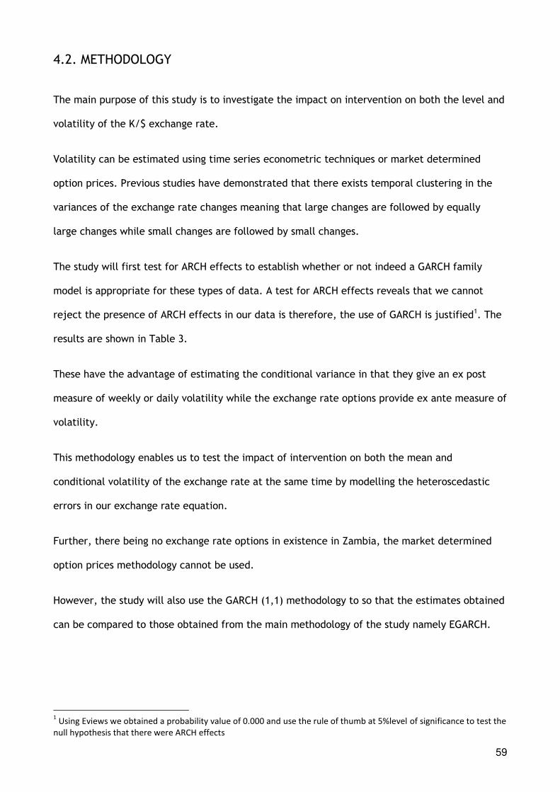
59

4.2. METHODOLOGY

The main purpose of this study is to investigate the impact on intervention on both the level and

volatility of the K/$ exchange rate.

Volatility can be estimated using time series econometric techniques or market determined

option prices. Previous studies have demonstrated that there exists temporal clustering in the

variances of the exchange rate changes meaning that large changes are followed by equally

large changes while small changes are followed by small changes.

The study will first test for ARCH effects to establish whether or not indeed a GARCH family

model is appropriate for these types of data. A test for ARCH effects reveals that we cannot

reject the presence of ARCH effects in our data is therefore, the use of GARCH is justified1. The

results are shown in Table 3.

These have the advantage of estimating the conditional variance in that they give an ex post

measure of weekly or daily volatility while the exchange rate options provide ex ante measure of

volatility.

This methodology enables us to test the impact of intervention on both the mean and

conditional volatility of the exchange rate at the same time by modelling the heteroscedastic

errors in our exchange rate equation.

Further, there being no exchange rate options in existence in Zambia, the market determined

option prices methodology cannot be used.

However, the study will also use the GARCH (1,1) methodology to so that the estimates obtained

can be compared to those obtained from the main methodology of the study namely EGARCH.

1 Using Eviews we obtained a probability value of 0.000 and use the rule of thumb at 5%level of significance to test the

null hypothesis that there were ARCH effects

60

THE EFFECTS OF BOZ’S INTERVENTION ON THE VOLATILITY OF THE

KWACHA

Most central bank‟s rationale for intervention is the „calming of disorderly‟ exchange rate

markets. In essence this entails arresting exchange rate volatility.

This study will adopt the Exponential GARCH (EGARCH) methodology proposed by Nelson (1991)

and used by Domac and Mendoza (2004) and Kim et al (2000) to model the overall effects of

intervention and the individual sales and purchases.

We propose the following process to model exchange rate returns and conditional volatility

assuming that the error terms are drawn from a double exponential (DE) distribution:

GARCH models are outperformed by fractionally integrated or long-memory processes and they

tend to underestimate the intervention effects in terms of volatility (Beine et al 2002 and Domac

and Mendoza 2004).

Further, EGARCH has a number of advantages over the ordinary GARCH models which include the

fact that the latter do not account for leverage effects and they imply that the impact of a

volatility shock disappears over time at an exponential rate (Beine et al (2002).

Enders (2004) revealed that EGARCH allows for asymmetric effects of shocks. In this case

purchases and sales of foreign exchange are supposed to have asymmetric effects on the

exchange rate. Unfortunately, GARCH being a symmetric model does not take that into account.

Another weakness of GARCH is that it is necessary to ensure that all of the estimated

coefficients are positive but EGARCH does not require non negativity constraints.

61

The E-GARCH allows for the inclusion of negative variables affecting volatility, which, in turn,

makes it possible to analyze, the sales and purchases, components of the intervention activities.

r t = ø0 + ø sale sale + ø

pur purch + є t

є t ~DE(0,σ 2) є t = є t σ t є t ~ iid (0,1)

In (σ 2

t ) = ω+ α (l є1t l) + (є 1t ) + β (In (σ 2

1t ) + sale + purchpurch ............. 4.1

Where

r t is equal to ΔInS t (is the log change in the K/$ exchange rate between period t and

t-1)

SALE is BOZ sales of $

PURCH is BOZ purchase of $

γ is a leverage parameter

PURCH will take a value of one when there is a purchase of dollars and zero otherwise, while

SALES takes a value of minus one for every sale of dollars.

This will ascertain the effects of BOZ intervention in frequency terms, by studying the response

of the variance to the number of times BOZ sells or buys at the same time.

The parameter α in the variance equation resembles the clustering effect showed by GARCH

models.

γ allows the variance to respond differently following equal magnitude negative or positive

shocks.

Volatility persistence is measured by β under the restriction that the estimate is smaller than

one to avoid an explosive behaviour of the variance.

To examine the asymmetric response of the variance to positive and negative

innovations, we employ the News Impact Curve (NIC) by Engle and Ng (1993), which is as follows:

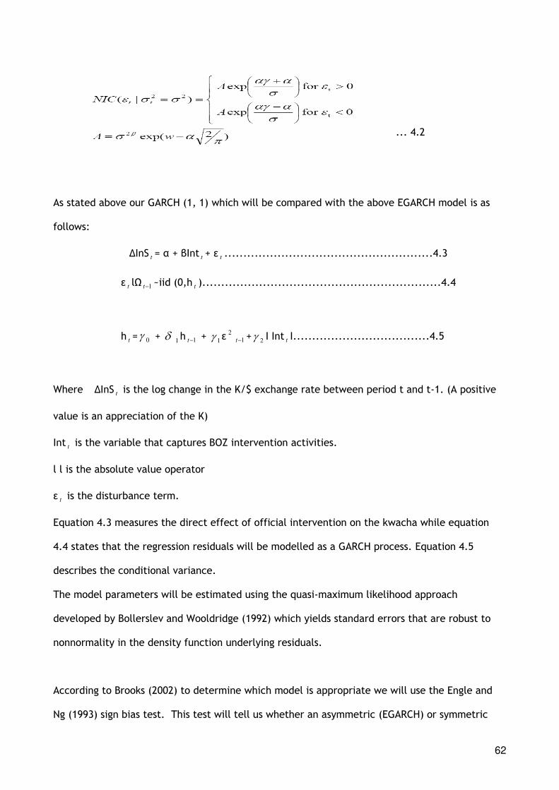
62

... 4.2

As stated above our GARCH (1, 1) which will be compared with the above EGARCH model is as

follows:

ΔInS t = α + βInt t + ε t .......................................................4.3

ε t lΩ 1t ~iid (0,h t )...............................................................4.4

h t = 0 +

1h

1t + 1

ε 2

1t +2

І Int t І....................................4.5

Where ΔInS t is the log change in the K/$ exchange rate between period t and t-1. (A positive

value is an appreciation of the K)

Int t is the variable that captures BOZ intervention activities.

l l is the absolute value operator

ε t is the disturbance term.

Equation 4.3 measures the direct effect of official intervention on the kwacha while equation

4.4 states that the regression residuals will be modelled as a GARCH process. Equation 4.5

describes the conditional variance.

The model parameters will be estimated using the quasi-maximum likelihood approach

developed by Bollerslev and Wooldridge (1992) which yields standard errors that are robust to

nonnormality in the density function underlying residuals.

According to Brooks (2002) to determine which model is appropriate we will use the Engle and

Ng (1993) sign bias test. This test will tell us whether an asymmetric (EGARCH) or symmetric

63

(GARCH) model is appropriate for our data series. This test is applied to the residuals of a

GARCH returns data. It is based on the significance of 𝜱1

in the following equation:

μ t = 𝜱0+ 𝜱

1S

1t + υ t

where υ t is an iid error term. If positive and negative shocks to μ1t impact differently upon the

conditional variance, then 𝜱1will be statistically significant.

Our prior expectation on this score is that sales and purchases will affect the condition variance

differently and therefore a model that care of this type of asymmetry, which in our case is

EGARCH should be more appropriate.

PRIOR EXPECTATIONS

Our expectation from this study is that BOZ‟s interventions are effective in reversing the

depreciating trend of the kwacha. Further we expect that volatility of the kwacha will increase

due to this intervention. As pointed out by Disyatat and Galati(2005) one would expect a priori

that foreign exchange intervention in emerging market countries may be more effective because

(i) the size of intervention relative to market turnover tends to be larger, (ii) the existence of

some form of capital controls limiting access to international capital markets gives central banks

in these countries greater leverage in the market, and (iii) the lower level of sophistication of

the domestic market along with stringent reporting requirements may endow central banks with

a greater informational advantage not only with respect to fundamentals but also aggregate

order flows and net open positions of major traders.

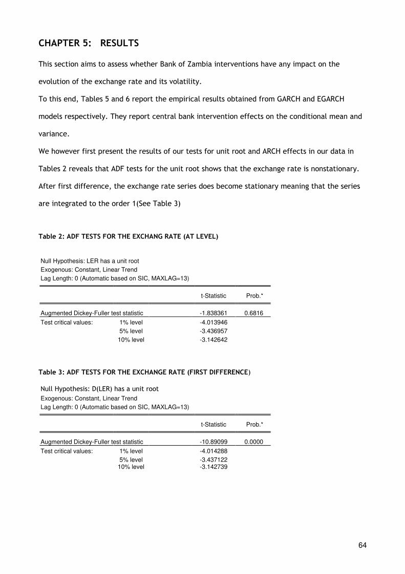
64

CHAPTER 5: RESULTS

This section aims to assess whether Bank of Zambia interventions have any impact on the

evolution of the exchange rate and its volatility.

To this end, Tables 5 and 6 report the empirical results obtained from GARCH and EGARCH

models respectively. They report central bank intervention effects on the conditional mean and

variance.

We however first present the results of our tests for unit root and ARCH effects in our data in

Tables 2 reveals that ADF tests for the unit root shows that the exchange rate is nonstationary.

After first difference, the exchange rate series does become stationary meaning that the series

are integrated to the order 1(See Table 3)

Table 2: ADF TESTS FOR THE EXCHANG RATE (AT LEVEL)

Null Hypothesis: LER has a unit root

Exogenous: Constant, Linear Trend

Lag Length: 0 (Automatic based on SIC, MAXLAG=13) t-Statistic Prob.*

Augmented Dickey-Fuller test statistic -1.838361 0.6816

Test critical values: 1% level -4.013946

5% level -3.436957

10% level -3.142642

Table 3: ADF TESTS FOR THE EXCHANGE RATE (FIRST DIFFERENCE)

Null Hypothesis: D(LER) has a unit root

Exogenous: Constant, Linear Trend

Lag Length: 0 (Automatic based on SIC, MAXLAG=13) t-Statistic Prob.*

Augmented Dickey-Fuller test statistic -10.89099 0.0000

Test critical values: 1% level -4.014288

5% level -3.437122 10% level -3.142739

65

ARCH tests are reported in Table 4 and stated earlier we could not reject the hypothesis that the series have ARCH effects. This lends support to the use of GARCH and EGARCH models.

Table 4: ARCH TEST

Heteroskedasticity Test: ARCH

F-statistic 56.80550 Prob. F(1,21) 0.0000

Obs*R-squared 16.79221 Prob. Chi-Square(1) 0.0000

Table 5. GARCH ESTIMATION OF THE EXCHANGE RATE. CONDITION MEAN

Coefficient Std. Error z-Statistic Prob. C 0.554223 0.094200 5.883495 0.0000

LS(-1) 0.039685 0.004702 8.439495 0.0000

LSALE -0.070994 0.010750 -6.603786 0.0000

LPURCH 0.009320 0.004084 2.282072 0.0225 CONDITION VARIANCE C -0.006426 0.003082 -2.085182 0.0371

RESID(-1)^2 1.063364 0.275898 3.854193 0.0001

GARCH(-1) 0.346587 0.093795 3.695174 0.0002

LSALE 0.000636 0.000294 2.166234 0.0303

LPURCH -0.000165 8.30E-05 -1.985239 0.0471

66

Table 6. EGARCH ESTIMATION OF THE EXCHANGE RATE CONDITIONAL MEAN

Coefficient Std. Error z-Statistic Prob.

C 0.280694 0.028485 9.854042 0.0000

LS(-1) 0.012793 0.002611 4.899596 0.0000

LSALE -0.026207 0.001299 -20.18152 0.0000

LPURCH -0.000938 0.002635 -0.356169 0.7217 CONDITIONAL VARIANCE

C(5) -7.916350 3.552413 -2.228443 0.0259

C(6) 0.805065 0.129104 6.235775 0.0000

C(7) 0.135139 0.094117 1.435861 0.1510

C(8) 0.761937 0.077636 9.814174 0.0000

C(9) 0.689722 0.375028 1.839121 0.0659

C(10) -0.292876 0.164917 -1.775899 0.0757

Figure 7: GARCH CONDITION VARIANCE

.00

.01

.02

.03

.04

.05

.06

.07

1996 1998 2000 2002 2004 2006 2008

Conditional variance

67

Figure 8: EGARCH CONDITION VARIANCE

Figure 9: EGARCH LS RESIDUALS

.00

.04

.08

.12

.16

.20

.24

.28

.32

1996 1998 2000 2002 2004 2006 2008

Conditional variance

-.3

-.2

-.1

.0

.1

.2

.3

1996 1998 2000 2002 2004 2006 2008

LS Residuals

68

EFFECTS OF INTERVENTION

5.2.1 MEAN EQUATION

We first examine the exchange rate mean level. In the GARCH model (Table 5) lsale (log of sale)

coefficient has a negative sign while the lpurch (purchase) coefficient has a positive sign. A

negative coefficient indicates that the exchange rate moves in the desired direction for

intervention, that is, a sale of $ depresses the value of the kwacha/$ exchange rate. It shows

that sales of $ reduce the mean of the exchange rate while a positive sign on purchases indicates

that purchasing $ increases the value of the exchange rate entailing a depreciation of the

kwacha. Both sales and purchases are also statistically significant.

It is difficult to understand the rationale behind BOZ‟s purchases of $ from the market if in this

case they lead to the depreciation of the kwacha. One would however, assume that the

objective is to build international reserves rather than to influence the exchange rate.

A similar study by Domac and Mendoza (2004) which was examining the intervention operations

of the Turkish and Mexican central banks makes the same observation that a net sale of $100

million appreciates the exchange rate by 0.08% and 0.20% in Mexico and Turkey respectively.

The study also observes that purchase of foreign exchange did not influence the exchange rate

at all.

In contrast to GARCH model, the EGARCH model‟s estimation results presented in Table 6 show

that the coefficients of both sales and purchases of $ are negatively signed. The results show

that BOZ sales and purchases activities both lead to an appreciation of the exchange rate.

Similar results in studies such as Kim et al (2000) make the same observation that the Reserve

Bank of Australia‟s intervention had moved the exchange rate in the desired direction of the

intervention. Fatum and Hutchison (1999) also find evidence that intervention does affect the

exchange rate. Our finding is also consistent with the related work of Catte et al (1999),

Humpage (1999) and Dominguez and Frankel (1993).

69

The interpretation of the negatively signed sales coefficient also means that when the BOZ is

selling $ it is getting kwacha from the market. This will therefore cause the exchange rate to

appreciate (decline). This is similar to the finding of Edison et al (2003) that when on those days

when official net sales of $ occurred in Australia, the USD/ Australian dollar tends to be rising.

In other words, the Reserve Bank of Australia sales the domestic currency this results in its

appreciation.

5.2.2. VARIANCE EQUATION

The pattern of effects of intervention on the conditional volatility is different from

that on the conditional mean. The sales coefficient in the GARCH model is positively signed and

it is statistically significant while the purchases coefficient is negatively signed and is

statistically insignificant. This shows that sales of dollars increase the variance of the exchange

rate while purchases of dollars reduce it. The 1

in this model is positively signed and is

statistically significant. This is in line with our expectation and therefore the GARCH model is

not the best for our study and instead the EGARCH model is best suited for this kind of study.

The ARCH and GARCH coefficients are typically close to unity indicating that volatility shocks in

the exchange rate are rather persistent.

Purchases of $ reduces the variance of the exchange rate. This shows that the central bank

actually achieves its objective of smoothing out exchange rate fluctuations. The study by

Dominguez (1998) of the Federal Reserve intervention activities makes a similar observation that

on general level central bank intervention increased exchange rate volatility. Similarly a study

on the effect of sales of foreign exchange on volatility by Kim et al (2000) using Australian data

too found that the conditional volatility of the exchange rate return was significantly raised.

Beine et al (2002) find strong evidence that central bank interventions tend to increase,

70

rather than to reduce, the volatility of exchange rates. This result is also consistent with the

major stream of the literature and specifically with Bonser-Neal and Tanner (1996) and Baillie

and Osterberg (1997a, b). It is consistent with the microstructure, according to which the

market tests the determination of the central banks just after the intervention occurs,

especially since volatility is usually found in the literature to be positively correlated with

turnover (see for instance Hartmann, 1998).

It appears the mere presence of the central bank in the foreign exchange market sends

ambiguous signals to market participants about both the intentions of the central bank and its

future monetary policy. This ambiguity can be interpreted to mean that the signalling channel is

the channel through which BOZ interventions in the foreign exchange market affects the

exchange.

71

CHAPTER 6. CONCLUSION

In this paper we investigate the impact of the Bank of Zambia‟s foreign exchange market

intervention on the level and volatility of the exchange rate namely the kwacha/ USD exchange

rate.

To measure this impact we use GARCH (1, 1) as well as EGARCH. To determine the

appropriateness of GARCH models we first test for ARCH effects in the data. Our ARCH presence

is subsequently confirmed and therefore we proceed to use GARCH (1, 1). GARCH (I, I) is

estimated using quasi maximum likelihood.

We also use Exponential GARCH which enables us to investigate both the overall effect of the

intervention and the individual effect of sales and purchases.

We use the sign bias test to test the best model between EGARCH and GARCH. We find that the

former model is better than the GARCH because of the asymmetrical impact of sales and

purchases of dollars on the exchange rate.

Empirical results from the GARCH model suggest that sales of foreign exchange lead to an

appreciation of the kwacha which is basically „leaning against the wind‟. In this regard, the

BOZ‟s goal of reversing a depreciation of the currency is achieved. In terms of volatility, the

GARCH results suggest that purchasing foreign exchange reduces volatility while selling it

increases volatility.

Our EGARCH results suggest that both sales and purchases of cause an appreciation of the

exchange rate while the impacts of such interventions on volatility are mixed. Purchases of

$ appear to reduce the volatility of the kwacha while sales of $ increase it.

There are a few possible directions for future research. First it would be important to know

exactly which channel/s the BOZ intervention activities affect the kwacha. Second it would be

important to distinguish between secret and publicly announced interventions so that their

72

different effects on the kwacha can be compared. Thirdly, it would be interesting to extend the

data set to include interventions on more than one exchange rate. This could include a Sub-

Saharan currency like the South African Rand which is pervasively used in the Zambian domestic

economy. This would increase the number of observed public interventions and would allow for a

more specific testing of hypotheses.

73

BIBLIOGRAPHY

Almekinders, G.J and Eijffinger, S.C.W.1994 The ineffectiveness of central Bank Intervention:

CentER Discussion Paper Series. Tilburg University No 94101 pp1-18

Aguilar, J and Nydahl, S. 2000. Central Bank intervention and Exchange Rates: The case of

Sweden. Journal of International Financial Markets, Institutions and Money 10 pp303-322

Aron, J and Eibadawi, I.A. 1992. Parallel Markets, the Foreign exchange Auction and Exchange

rate Unification in Zambia. World Bank Working Paper WPS 909

Bacchetta, P and Van Wincoop, E. 2006. The American Economic Review Vol. 96 No3 pp552- 576

Bank for International Settlements (BIS). 2007. Foreign exchange and derivates market activity.

Triennial Central Bank Survey.

Bank of Zambia, 2008. Annual Financial Reports

Beine, M. et al 2002. Central Bank Intervention and Foreign Exchange Rates: New evidence from

FIGARCH estimations. Journal of International Money and Finance 21 pp 115-114.

Bordo, M and Scwartz, A. 1991. What has Foreign Exchange Market intervention since the Plaza

Agreement accomplished? Open Economies Review 2. Pp39-64

Bonser- Neal, C. 1996. Does Central Bank intervention stabilize foreign exchange rates? Federal

Reserve Bank of Kansas City.

Brooks , C. 2002. Introductory Econometrics for Finance. CUP

74

Canales-Kriljenko, J.I.1995. Foreign exchange intervention in developing and transition

economies: Results of a survey IMF Working Paper WP/03/95

Copeland, L .2008. Exchange Rates and International Finance (5th Edition). Prentice Hall

Financial Times.

Disyatat, P and Galati, G 2005. The effectiveness of foreign Exchange intervention in emerging

market countries: Evidence from the Czech Koruna. BIS Working Paper NO 172

Domac, I and Mendoza, A. 2004.Is there room for foreign exchange interventions under an

inflation targeting framework? Evidence from Mexico and Turkey. World Bank Policy Research

Working Paper 3288

Dominguez, K.M., 1998. Central Bank Intervention and Exchange rate Volatility. Journal of

International Money and Finance, 17 161-190.

Dominguez, K.M. 1990 Market Responses to coordinated central bank intervention. Carnegie –

Rochester Conference Series on Public Policy 32 pp 121-164

Dominguez, K.M. 2006. When do Central Bank Intervention Influence intra-daily and longer -term

exchange rate movements. Journal of International Money and Finance 25 pp 1051-1071

Dominguez, K.M. 2003. The Market Microstructure of Central Bank Intervention. Journal of

International Economics 59 pp 25-45

Dominguez, K.M. 2003. Foreign Exchange Intervention: Did it work in the 1990s. Institute of

International Economics

75

Dominguez,K.M and Frankel, J.A. 1993A. Does Foreign Exchange Intervention work? Washington

D.C. Institute of International Economics

Dominguez,K.M and Frankel, J.A. 1993B. Does Foreign Exchange Intervention Matter? The

Portfolio Effect. American Economic Review vol 83 No 5 pp 1356-1369

Enders, W. 2004. Applied Econometric Time Series ( 2nd Edition) John Wiley & Sons Inc

Edison, H., Cashin, P. & Liang, H., 2003. Foreign exchange intervention and the Australian

Dollar: Has it mattered? IMF Working paper WP/03/99.

Fatum, R. and Hutchison, M., 1999B. Is sterilized foreign exchange intervention

effective after all: An event study approach?

Fatum, R and Hutchison, M. 1999A. Is intervention a signal of future monetary policy? Evidence

from the Federal Funds Futures Market. Journal of Money, Credit and Banking Vol 31 No1 pp 54-

69.

Frenkel, M et al 2005. The effects of Japanese foreign exchange market intervention on the

Yen/US Dollar exchange rate volatility. International Review of Economics and Finance No 14

page 27-39

Ghosh, A.R. 1992. Is it signalling? Exchange Intervention and the dollar- Deutschemark Rate.

Journal of International Economics 32 pp 201-220 North –Holland.

Hallwood,C.P and MacDonald, R. 3rd edition International Money and Finance Blackwell

Publishers.

76

Hardy, D.C, 1997. Market information and signaling in central bank operations or how often

should a central bank intervene? IMF Working Paper 28

Humpage, O.F. 1999. US Intervention: Assessing the probability of success. Journal of Money,

Credit and Banking. Volume 31 No 4 pp731-747

Hoshikawa, T. 2008. The causal relationship between foreign exchange Intervention and

exchange rate. Applied economics letters. London Vol. 15 Iss.7

Hoshikawa, T 2008. The effect on intervention frequency on the foreign

Exchange market: The Japanese experience. Journal of International Money and Finance Vol.27

Iss. 4 p 547.

IMF country Report. 2008. No 08/187 Washington. D.C.

Kaminsky, G.L and Lewis, K.K. 1996. Does foreign Exchange Intervention signal monetary policy.

Journal of Monetary Economics 37 pp 285-312.

Kaminsky, G. and Lewis, K. 1996. Does Foreign Exchange Intervention Signal future monetary

policy? Journal of Monetary Economics 37 285- 312.

Kim, S et al. 2000. Central Bank intervention and exchange rate volatility – Australian Evidence.

Journal of International and Financial Markets Institutions and Money 10(210) pp381-405.

Loopsesko, B.E. 1984. Relationships among Exchange Rate intervention and interest rates: An

empirical investigation. Journal of International Money and Finance 3(3) pp 257-77

Mussa, M 1981. The Role of Official Intervention. Group of Thirty New York

77

Neely, C.J. 2000. The practice of central bank intervention: Looking around the Hood .The

Federal Reserve Bank of St. Louis Working Paper Series 28

Neely, C. 2005. An analysis of Recent studies of the effect of foreign exchange intervention.

Federal Reserve Bank of St. Louis Review 87(6) pp 685-717

Pilbeam, K 2006. International Finance (3rd edition).Palgrave Macmillan

Sarantis, N., 2006. On the short-term predictability of exchange rates:

A BVAR time-varying parameters approach. Journal of Banking and Finance 30, 2257-2279

Sarno, L and Taylor, M.P. 2001. Official intervention in the Foreign Exchange Market: Is it

effective and if so how does it work? Journal of Economic Literature. Vol 39 N0 3 PP 839-868

Sarno, L and Taylor, M.P. 2008. The Economics of Exchange Rates. Cambridge University Press.

Cambridge

Simatachela, M. 2004. Financial Sector Reforms and Monetary Policy in Zambia. PhD dissertation

Department of Economics Goteborg University- Sweden.

78

APPENDIX 1

GARCH OUTPUT

Dependent Variable: D(LS) Method: ML - ARCH (Marquardt) - Normal distribution Date: 05/11/09 Time: 17:49 Sample (adjusted): 1995M03 2008M12 Included observations: 166 after adjustments Convergence achieved after 40 iterations Presample variance: backcast (parameter = 0.7) GARCH = C(5) + C(6)*RESID(-1)^2 + C(7)*GARCH(-1) + C(8)*LSALE + C(9)*LPURCH

Coefficie

nt Std. Error z-Statistic Prob. C 0.554223 0.094200 5.883495 0.0000

LS(-1) 0.039685 0.004702 8.439495 0.0000

LSALE -

0.070994 0.010750 -6.603786 0.0000 LPURCH 0.009320 0.004084 2.282072 0.0225

Variance Equation

C -

0.006426 0.003082 -2.085182 0.0371 RESID(-1)^2 1.063364 0.275898 3.854193 0.0001 GARCH(-1) 0.346587 0.093795 3.695174 0.0002

LSALE 0.000636 0.000294 2.166234 0.0303

LPURCH -

0.000165 8.30E-05 -1.985239 0.0471

R-squared -

0.081655 Mean dependent var 0.011131

Adjusted R-squared -

0.136771 S.D. dependent var 0.047009 S.E. of regression 0.050121 Akaike info criterion -3.569802 Sum squared resid 0.394405 Schwarz criterion -3.401080 Log likelihood 305.2936 Hannan-Quinn criter. -3.501317 Durbin-Watson stat 1.579765

79

EGARCH OUPTUT Dependent Variable: D(LS) Method: ML - ARCH (Marquardt) - Normal distribution Date: 05/11/09 Time: 17:51 Sample (adjusted): 1995M03 2008M12 Included observations: 166 after adjustments Failure to improve Likelihood after 26 iterations Presample variance: backcast (parameter = 0.7) LOG(GARCH) = C(5) + C(6)*ABS(RESID(-1)/@SQRT(GARCH(-1))) + C(7) *RESID(-1)/@SQRT(GARCH(-1)) + C(8)*LOG(GARCH(-1)) + C(9) *LSALE + C(10)*LPURCH

Coefficie

nt Std. Error z-Statistic Prob. C 0.280694 0.028485 9.854042 0.0000

LS(-1) 0.012793 0.002611 4.899596 0.0000

LSALE -

0.026207 0.001299 -20.18152 0.0000

LPURCH -

0.000938 0.002635 -0.356169 0.7217 Variance Equation

C(5) -

7.916350 3.552413 -2.228443 0.0259 C(6) 0.805065 0.129104 6.235775 0.0000 C(7) 0.135139 0.094117 1.435861 0.1510 C(8) 0.761937 0.077636 9.814174 0.0000 C(9) 0.689722 0.375028 1.839121 0.0659

C(10) -

0.292876 0.164917 -1.775899 0.0757 R-squared 0.004204 Mean dependent var 0.011131

Adjusted R-squared -

0.053245 S.D. dependent var 0.047009 S.E. of regression 0.048245 Akaike info criterion -3.582352 Sum squared resid 0.363098 Schwarz criterion -3.394883 Log likelihood 307.3352 Hannan-Quinn criter. -3.506257 F-statistic 0.073182 Durbin-Watson stat 1.665371 Prob(F-statistic) 0.999893

80

Dependent Variable: D(LS) Method: ML - ARCH (Marquardt) - Generalized error distribution (GED) Date: 05/11/09 Time: 17:52 Sample (adjusted): 1995M03 2008M12 Included observations: 166 after adjustments Failure to improve Likelihood after 5 iterations Presample variance: backcast (parameter = 0.7) LOG(GARCH) = C(5) + C(6)*ABS(RESID(-1)/@SQRT(GARCH(-1))) + C(7) *RESID(-1)/@SQRT(GARCH(-1)) + C(8)*LOG(GARCH(-1)) + C(9) *LSALE + C(10)*LPURCH

Coefficie

nt Std. Error z-Statistic Prob. C 0.465797 0.072748 6.402926 0.0000

LS(-1) 0.025160 0.008930 2.817417 0.0048

LSALE -

0.055084 0.000818 -67.36994 0.0000 LPURCH 0.007982 0.000625 12.78027 0.0000

Variance Equation

C(5) -

4.264120 5.442462 -0.783491 0.4333 C(6) 0.675041 0.254116 2.656427 0.0079

C(7) -

0.036944 0.174159 -0.212126 0.8320 C(8) 0.544335 0.149915 3.630964 0.0003 C(9) 0.214197 0.574438 0.372880 0.7092

C(10) -

0.166998 0.254078 -0.657270 0.5110 GED PARAMETER 1.147957 0.135305 8.484190 0.0000

R-squared -

0.035808 Mean dependent var 0.011131

Adjusted R-squared -

0.102634 S.D. dependent var 0.047009 S.E. of regression 0.049363 Akaike info criterion -3.749506 Sum squared resid 0.377688 Schwarz criterion -3.543290 Log likelihood 322.2090 Hannan-Quinn criter. -3.665802 Durbin-Watson stat 1.624748

81

DATE EXCHANGE RATE SALE PURCH CMSALE CMPURCH

Jan-95 688.65 36,800.00 0.00 36,800.00

-

Feb-95 769.57 67,200.00 0.00 104,000.00

-

Mar-95 797.08 27,100.00 7,900.00 131,100.00

7,900.00

Apr-95 802.06 30,200.00 0.00 161,300.00

7,900.00

May-95 829 35,900.00 0.00 197,200.00

7,900.00

Jun-95 893.51 47,500.00 0.00 244,700.00

7,900.00

Jul-95 927.71 29,600.00 200.00 274,300.00

8,100.00

Aug-95 930.78 31,300.00 700.00 305,600.00

8,800.00

Sep-95 932.68 36,100.00 0.00 341,700.00

8,800.00

Oct-95 932.68 28,300.00 0.00 370,000.00

8,800.00

Nov-95 927.92 41,100.00 0.00 411,100.00

8,800.00

Dec-95 937.79 62,100.00 40,700.00 473,200.00

49,500.00

Jan-96 982.19 37,000.00 0.00 510,200.00

49,500.00

Feb-96 992.2 40,000.00 0.00 550,200.00

49,500.00

Mar-96 1135.47 28,600.00 0.00 578,800.00

49,500.00

Apr-96 1282.9 31,400.00 7,100.00 610,200.00

56,600.00

May-96 1240.9 100.00 24,500.00 610,300.00

81,100.00

Jun-96 1241.03 600.00 13,010.00 610,900.00

94,110.00

Jul-96 1259.12 0.00 2,000.00 610,900.00

96,110.00

Aug-96 1267.86 0.00 9,990.00 610,900.00

106,100.00

Sep-96 1266.72 0.00 39,485.00 610,900.00

145,585.00

Oct-96 1269.15 4,200.00 9,900.00 615,100.00

155,485.00

Nov-96 1269.83 12,700.00 5,135.00 627,800.00

160,620.00

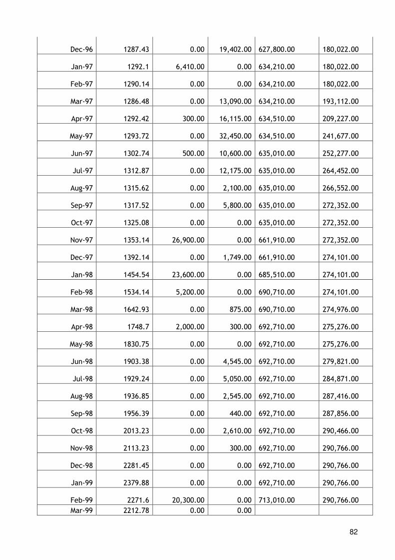
82

Dec-96 1287.43 0.00 19,402.00 627,800.00

180,022.00

Jan-97 1292.1 6,410.00 0.00 634,210.00

180,022.00

Feb-97 1290.14 0.00 0.00 634,210.00

180,022.00

Mar-97 1286.48 0.00 13,090.00 634,210.00

193,112.00

Apr-97 1292.42 300.00 16,115.00 634,510.00

209,227.00

May-97 1293.72 0.00 32,450.00 634,510.00

241,677.00

Jun-97 1302.74 500.00 10,600.00 635,010.00

252,277.00

Jul-97 1312.87 0.00 12,175.00 635,010.00

264,452.00

Aug-97 1315.62 0.00 2,100.00 635,010.00

266,552.00

Sep-97 1317.52 0.00 5,800.00 635,010.00

272,352.00

Oct-97 1325.08 0.00 0.00 635,010.00

272,352.00

Nov-97 1353.14 26,900.00 0.00 661,910.00

272,352.00

Dec-97 1392.14 0.00 1,749.00 661,910.00

274,101.00

Jan-98 1454.54 23,600.00 0.00 685,510.00

274,101.00

Feb-98 1534.14 5,200.00 0.00 690,710.00

274,101.00

Mar-98 1642.93 0.00 875.00 690,710.00

274,976.00

Apr-98 1748.7 2,000.00 300.00 692,710.00

275,276.00

May-98 1830.75 0.00 0.00 692,710.00

275,276.00

Jun-98 1903.38 0.00 4,545.00 692,710.00

279,821.00

Jul-98 1929.24 0.00 5,050.00 692,710.00

284,871.00

Aug-98 1936.85 0.00 2,545.00 692,710.00

287,416.00

Sep-98 1956.39 0.00 440.00 692,710.00

287,856.00

Oct-98 2013.23 0.00 2,610.00 692,710.00

290,466.00

Nov-98 2113.23 0.00 300.00 692,710.00

290,766.00

Dec-98 2281.45 0.00 0.00 692,710.00

290,766.00

Jan-99 2379.88 0.00 0.00 692,710.00

290,766.00

Feb-99 2271.6 20,300.00 0.00 713,010.00

290,766.00

Mar-99 2212.78 0.00 0.00

83

713,010.00 290,766.00

Apr-99 2325.62 0.00 750.00 713,010.00

291,516.00

May-99 2389.16 0.00 0.00 713,010.00

291,516.00

Jun-99 2418.8 0.00 7,500.00 713,010.00

299,016.00

Jul-99 2431.55 5,000.00 5,400.00 718,010.00

304,416.00

Aug-99 2397.97 0.00 1,300.00 718,010.00

305,716.00

Sep-99 2381.41 0.00 4,070.00 718,010.00

309,786.00

Oct-99 2401.45 0.00 1,000.00 718,010.00

310,786.00

Nov-99 2452.42 0.00 0.00 718,010.00

310,786.00

Dec-99 2593.59 626.00 0.00 718,636.00

310,786.00

Jan-00 2653.88 0.00 0.00 718,636.00

310,786.00

Feb-00 2734.46 1,400.00 15,000.00 720,036.00

325,786.00

Mar-00 2754.84 12,400.00 14,200.00 732,436.00

339,986.00

Apr-00 2801.39 15,000.00 1,000.00 747,436.00

340,986.00

May-00 2857.76 0.00 0.00 747,436.00

340,986.00

Jun-00 2939.94 0.00 300.00 747,436.00

341,286.00

Jul-00 3083.9 0.00 0.00 747,436.00

341,286.00

Aug-00 3204.67 0.00 0.00 747,436.00

341,286.00

Sep-00 3244.11 0.00 17,000.00 747,436.00

358,286.00

Oct-00 3338.01 0.00 0.00 747,436.00

358,286.00

Nov-00 3608.42 0.00 0.00 747,436.00

358,286.00

Dec-00 4108.75 0.00 1,500.00 747,436.00

359,786.00

Jan-01 4024.53 7,600.00 7,000.00 755,036.00

366,786.00

Feb-01 3602.66 32,600.00 0.00 787,636.00

366,786.00

Mar-01 3349.59 26,550.00 4,790.00 814,186.00

371,576.00

Apr-01 3104.48 36,700.00 300.00 850,886.00

371,876.00

May-01 3323.04 32,850.00 2,090.00 883,736.00

373,966.00

Jun-01 3604.46 14,050.00 0.00 897,786.00

373,966.00

84

Jul-01 3685.3 36,850.00 6,800.00 934,636.00

380,766.00

Aug-01 3594.3 36,150.00 3,600.00 970,786.00

384,366.00

Sep-01 3678.19 22,400.00 0.00 993,186.00

384,366.00

Oct-01 3743.49 37,150.00 0.00 1,030,336.00

384,366.00

Nov-01 3800.85 37,050.00 0.00 1,067,386.00

384,366.00

Dec-01 3820.33 20,800.00 0.00 1,088,186.00

384,366.00

Jan-02 3848.65 22,300.00 3,600.00 1,110,486.00

387,966.00

Feb-02 3904.25 16,500.00 0.00 1,126,986.00

387,966.00

Mar-02 3930.72 20,830.00 0.00 1,147,816.00

387,966.00

Apr-02 3939.03 12,300.00 0.00 1,160,116.00

387,966.00

May-02 4097.61 28,000.00 0.00 1,188,116.00

387,966.00

Jun-02 4354.66 21,900.00 200.00 1,210,016.00

388,166.00

Jul-02 4499.23 23,900.00 350.00 1,233,916.00

388,516.00

Aug-02 4492.73 30,500.00 3,500.00 1,264,416.00

392,016.00

Sep-02 5619.21 16,100.00 7,300.00 1,280,516.00

399,316.00

Oct-02 4603.27 34,400.00 1,100.00 1,314,916.00

400,416.00

Nov-02 4753.73 27,199.00 0.00 1,342,115.00

400,416.00

Dec-02 4740.05 32,700.00 0.00 1,374,815.00

400,416.00

Jan-03 4410.96 25,600.00 0.00 1,400,415.00

400,416.00

Feb-03 4668.71 23,200.00 300.00 1,423,615.00

400,716.00

Mar-03 4877.52 11,990.00 1,000.00 1,435,605.00

401,716.00

Apr-03 4866.4 18,650.00 8,100.00 1,454,255.00

409,816.00

May-03 4824.04 14,800.00 6,700.00 1,469,055.00

416,516.00

Jun-03 4847.04 17,000.00 3,500.00 1,486,055.00

420,016.00

Jul-03 4779.32 12,700.00 6,500.00 1,498,755.00

426,516.00

Aug-03 4698.57 0.00 4,410.00 1,498,755.00

430,926.00

Sep-03 4745.65 0.00 0.00 1,498,755.00

430,926.00

Oct-03 4752.02 0.00 2,000.00

85

1,498,755.00 432,926.00

Nov-03 4751.27 0.00 0.00 1,498,755.00

432,926.00

Dec-03 4577.75 0.00 1,000.00 1,498,755.00

433,926.00

Jan-04 4767.64 0.00 0.00 1,498,755.00

433,926.00

Feb-04 4762.51 0.00 3,000.00 1,498,755.00

436,926.00

Mar-04 4722.06 0.00 11,500.00 1,498,755.00

448,426.00

Apr-04 4734.95 0.00 9,800.00 1,498,755.00

458,226.00

May-04 4754.58 0.00 12,198.50 1,498,755.00

470,424.50

Jun-04 4832.62 0.00 11,551.90 1,498,755.00

481,976.40

Jul-04 4783.13 0.00 9,500.00 1,498,755.00

491,476.40

Aug-04 4787.26 0.00 7,200.00 1,498,755.00

498,676.40

Sep-04 4856.29 0.00 25,000.00 1,498,755.00

523,676.40

Oct-04 4896.31 3,500.00 0.00 1,502,255.00

523,676.40

Nov-04 4797.64 4,000.00 0.00 1,506,255.00

523,676.40

Dec-04 4651.51 0.00 1,000.00 1,506,255.00

524,676.40

Jan-05 4,785.12 0.00 14,000.00 1,506,255.00

538,676.40

Feb-05 4,758.50 0.00 2,000.00 1,506,255.00

540,676.40

Mar-05 4,710.58 0.00 16,900.00 1,506,255.00

557,576.40

Apr-05 4,675.15 0.00 23,000.00 1,506,255.00

580,576.40

May-05 4,691.79 0.00 12,000.00 1,506,255.00

592,576.40

Jun-05 4,685.77 0.00 17,700.00 1,506,255.00

610,276.40

Jul-05 4,624.46 200.00 31,000.00 1,506,455.00

641,276.40

Aug-05 4,401.88 0.00 5,500.00 1,506,455.00

646,776.40

Sep-05 4,439.67 0.00 0.00 1,506,455.00

646,776.40

Oct-05 4,346.08 0.00 0.00 1,506,455.00

646,776.40

Nov-05 4,026.68 0.00 0.00 1,506,455.00

646,776.40

Dec-05 3,416.34 3,000.00 5,000.00 1,509,455.00

651,776.40

Jan-06 3,363.72 0.00 12,000.00 1,509,455.00

663,776.40

86

Feb-06 3,289.61 0.00 0.00 1,509,455.00

663,776.40

Mar-06 3,294.74 0.00 0.00 1,509,455.00

663,776.40

Apr-06 3,201.50 0.00 42,500.00 1,509,455.00

706,276.40

May-06 3,184.97 7,000.00 15,500.00 1,516,455.00

721,776.40

Jun-06 3,470.61 0.00 8,500.00 1,516,455.00

730,276.40

Jul-06 3,546.72 5,000.00 0.00 1,521,455.00

730,276.40

Aug-06 3,883.95 28,000.00 12,500.00 1,549,455.00

742,776.40

Sep-06 4,046.46 16,000.00 90,800.00 1,565,455.00

833,576.40

Oct-06 3,835.17 14,500.00 39,000.00 1,579,955.00

872,576.40

Nov-06 3,984.97 7,000.00 0.00 1,586,955.00

872,576.40

Dec-06 4,127.83 36,200.00 0.00 1,623,155.00

872,576.40

Jan-07 4,221.06 21,500.00 0.00 1,644,655.00

872,576.40

Feb-07 4,254.02 4,500.00 0.00 1,649,155.00

872,576.40

Mar-07 4,258.53 8,000.00 42,500.00 1,657,155.00

915,076.40

Apr-07 4,161.47 9,000.00 22,500.00 1,666,155.00

937,576.40

May-07 4,013.82 0.00 34,408.00 1,666,155.00

971,984.40

Jun-07 3,888.11 0.00 10,000.00 1,666,155.00

981,984.40

Jul-07 3,823.05 5,000.00 6,000.00 1,671,155.00

987,984.40

Aug-07 4,013.08 25,500.00 0.00 1,696,655.00

987,984.40

Sep-07 3,960.70 3,000.00 12,500.00 1,699,655.00

1,000,484.40

Oct-07 3,831.36 0.00 3,000.00 1,699,655.00

1,003,484.40

Nov-07 3,766.67 6,000.00 11,000.00 1,705,655.00

1,014,484.40

Dec-07 3,836.88 9,500.00 0.00 1,715,155.00

1,014,484.40

Jan-08 3,792.78 11,000.00 0.00 1,726,155.00

1,014,484.40

Feb-08 3,753.59 0.00 0.00 1,726,155.00

1,014,484.40

Mar-08 3,668.91 2,000.00 13,000.00 1,728,155.00

1,027,484.40

Apr-08 3,519.41 0.00 17,500.00 1,728,155.00

1,044,984.40

May-08 3,399.20 15,500.00 7,000.00

87

1,743,655.00 1,051,984.40

Jun-08 3,249.70 8,000.00 15,500.00 1,751,655.00

1,067,484.40

Jul-08 3,393.37 32,500.00 0.00 1,784,155.00

1,067,484.40

Aug-08 3,452.79 5,000.00 0.00 1,789,155.00

1,067,484.40

Sep-08 3,539.85 22,500.00 3,500.00 1,811,655.00

1,070,984.40

Oct-08 4,044.33 48,000.00 0.00 1,859,655.00

1,070,984.40

Nov-08 4,256.98 15,000.00 3,500.00 1,874,655.00

1,074,484.40

Dec-08 4,882.97 70,000.00 2,000.00 1,944,655.00

1,076,484.40

APPENDIX 3.

DATE K/$ DATE k/$

Jan-98 1454.54 Aug-03 4698.57

Feb-98 1534.14 Sep-03 4745.65

Mar-98 1642.93 Oct-03 4752.02

Apr-98 1748.7 Nov-03 4751.27

May-98 1830.75 Dec-03 4577.75

Jun-98 1903.38 Jan-04 4767.64

Jul-98 1929.24 Feb-04 4762.51

Aug-98 1936.85 Mar-04 4722.06

Sep-98 1956.39 Apr-04 4734.95

Oct-98 2013.23 May-04 4754.58

Nov-98 2113.23 Jun-04 4832.62

Dec-98 2281.45 Jul-04 4783.13

Jan-99 2379.88 Aug-04 4787.26

Feb-99 2271.6 Sep-04 4856.29

Mar-99 2212.78 Oct-04 4896.31

Apr-99 2325.62 Nov-04 4797.64

May-99 2389.16 Dec-04 4651.51

Jun-99 2418.8 Jan-05 4,785.12

Jul-99 2431.55 Feb-05 4,758.50

Aug-99 2397.97 Mar-05 4,710.58

Sep-99 2381.41 Apr-05 4,675.15

Oct-99 2401.45 May-05 4,691.79

Nov-99 2452.42 Jun-05 4,685.77

Dec-99 2593.59 Jul-05 4,624.46

Jan-00 2653.88 Aug-05 4,401.88

Feb-00 2734.46 Sep-05 4,439.67

Mar-00 2754.84 Oct-05 4,346.08

Apr-00 2801.39 Nov-05 4,026.68

May-00 2857.76 Dec-05 3,416.34

88

Jun-00 2939.94 Jan-06 3,363.72

Jul-00 3083.9 Feb-06 3,289.61

Aug-00 3204.67 Mar-06 3,294.74

Sep-00 3244.11 Apr-06 3,201.50

Oct-00 3338.01 May-06 3,184.97

Nov-00 3608.42 Jun-06 3,470.61

Dec-00 4108.75 Jul-06 3,546.72

Jan-01 4024.53 Aug-06 3,883.95

Feb-01 3602.66 Sep-06 4,046.46

Mar-01 3349.59 Oct-06 3,835.17

Apr-01 3104.48 Nov-06 3,984.97

May-01 3323.04 Dec-06 4,127.83

Jun-01 3604.46 Jan-07 4,221.06

Jul-01 3685.3 Feb-07 4,254.02

Aug-01 3594.3 Mar-07 4,258.53

Sep-01 3678.19 Apr-07 4,161.47

Oct-01 3743.49 May-07 4,013.82

Nov-01 3800.85 Jun-07 3,888.11

Dec-01 3820.33 Jul-07 3,823.05

Jan-02 3848.65 Aug-07 4,013.08

Feb-02 3904.25 Sep-07 3,960.70

Mar-02 3930.72 Oct-07 3,831.36

Apr-02 3939.03 Nov-07 3,766.67

May-02 4097.61 Dec-07 3,836.88

Jun-02 4354.66 Jan-08 3,792.78

Jul-02 4499.23 Feb-08 3,753.59

Aug-02 4492.73 Mar-08 3,668.91

Sep-02 5619.21 Apr-08 3,519.41

Oct-02 4603.27 May-08 3,399.20

Nov-02 4753.73 Jun-08 3,249.70

Dec-02 4740.05 Jul-08 3,393.37

Jan-03 4410.96 Aug-08 3,452.79

Feb-03 4668.71 Sep-08 3,539.85

Mar-03 4877.52 Oct-08 4,044.33

Apr-03 4866.4 Nov-08 4,256.98

May-03 4824.04 Dec-08 4,882.97

Jun-03 4847.04

Jul-03 4779.32