The Impact of a Three-Tier Formulary on Demand Response for Prescription...

The Impact of a Three-Tier Formulary onDemand Response for Prescription Drugs

HAIDEN A. HUSKAMP

Department of Health Care PolicyHarvard Medical School

Boston, MA [email protected]

RICHARD G. FRANK

Department of Health Care PolicyHarvard Medical School and NBER

KIMBERLY A. MCGUIGAN

Pfizer, Inc.

YUTING ZHANG

Harvard University

A large number of health plans and employers have adopted three-tier pre-scription drug formularies in an effort to control rising prescription drugcosts. We assessed the behavioral response to three-tier adoption by estimatingeconometric models of the probability of selecting drugs assigned to the thirdtier with the highest co-payment requirement and changes in expected out-of-pocket (OOP) spending. We concluded that implementation of the three-tierformulary resulted in some shifting of costs from the plan to enrollees and somebargaining power gained for the payer, with plan savings from manufacturerrebates a likely result.

1. Introduction

In recent years, spending on prescription drugs has grown rapidly,causing new policy and management attention to be focused on that partof health care spending (Berndt, 2003). In response to drug cost increases,

We are grateful for funding from the Robert Wood Johnson Foundation’s Changes inHealth Care Financing and Organization Program, the National Institute for Mental Health(1 K01 MH66109), the Agency for HealthCare Research and Quality (5 P01 HS10803-2), and the Alfred P. Sloan Foundation. The authors are grateful to Patricia Deverka,Arnold Epstein, Robert Epstein, Will Manning, Tom McGuire, Joseph Newhouse, and threeanonymous reviewers for many constructive suggestions. Boris Fainstein and KathrynTrainor provided expert programming.

c© 2005 Blackwell Publishing, 350 Main Street, Malden, MA 02148, USA, and 9600 Garsington Road,Oxford OX4 2DQ, UK.Journal of Economics & Management Strategy, Volume 14, Number 3, Fall 2005, 729–753

730 Journal of Economics & Management Strategy

many employers, health plans, and pharmacy benefit managers (PBMs)(i.e., vendors that specialize in managing pharmacy benefits), haveadopted various management techniques, including incentive formu-laries. A formulary is a list of drugs categorized by the therapeuticuses of specific agents. Under an incentive formulary, a set of economicincentives for consumers of drugs accompanies the drug list. Incentiveformularies have particular policy significance because they are likely tobe used as a means of controlling benefit costs under the new MedicarePart D drug benefit to be implemented in 2006.

The most common type of incentive formulary is the three-tierformulary. Approximately, two-thirds of privately insured workers andtheir dependents had prescription drug coverage that used three-tierco-payment structures in 2004 (Kaiser Family Foundation, 2004). Three-tier formularies encourage consumers to choose drugs that are lessexpensive for the plan. Consumers using generic drugs—the first tier—pay the lowest OOP costs (e.g., $10) for a prescription; users of preferredbrand-name drugs—the second tier—pay a higher OOP price (e.g.,$20) and users of non preferred brand-name drugs—the third tier—pay the highest level of cost-sharing (e.g., $35). In contrast to a closedformulary (an incentive formulary that provides no coverage for drugsnot preferred by the plan), virtually all drugs are covered under a three-tier formulary. However, the OOP prices are such that consumers areencouraged to use the drugs preferred by the health plan. The ability toinfluence demand through the use of financial incentives to consumersbestows some bargaining power on the PBM to negotiate favorableprices with prescription-drug manufacturers (Frank, 2001).

In the analysis reported below, we make use of a natural experi-ment in the implementation of a three-tier co-payment structure to studydemand response for drugs in three commonly used therapeutic cate-gories. We examine the extent to which patients change to a medicationof a lower tier in response to a relative out-of-pocket (OOP) price changefor selected drugs in each therapeutic class. We also examine changesin expected OOP spending among users of the medications.

The paper is organized into five additional sections: backgroundon three-tier formularies, a summary of the relevant literature, a descrip-tion of our empirical approach, a summary of results, and discussion ofthose results.

2. Background

Pharmaceutical manufacturers have long been thought to competeby trying to differentiate their products from those of rival pro-ducers (Scherer, 1993; Task Force on Prescription Drugs, 1968).

Impact of a Three-Tier Formulary 731

Prescription-drug products within a therapeutic class are often similarin terms of their active ingredients but can differ in terms of side effects,toxicity, range of therapeutic indications, and mode of administration(e.g., once a day vs. two to three times a day). The industry competesactively to highlight differences between products in the minds ofdoctors and consumers alike. In 2000, branded drug manufacturersdevoted 14% of sales revenues to promotion of their products, of whichabout 15% was for direct-to-consumer advertising (Rosenthal et al.,2002). Successful product differentiation serves to decrease the priceelasticity of demand and reduce price competition in the market. As aresult, equilibrium market prices in more highly differentiated marketsare typically higher (Tirole, 1988; Viscusi et al., 2000).

Incentive formularies can help offset the differentiation strategiesof manufacturers. A three-tier co-payment structure introduces priceas a basis for consumer choice instead of allowing competition within atherapeutic drug class to be based primarily on attributes of the products(Ellison et al., 1997). By creating price differentials between productsthat may have similar mechanisms of action and thus be substitutes inthe production of health, PBMs through their formularies may increaseconsumers’ ability to respond to price and thereby enhance the PBM’sown bargaining power with manufacturers.

In 2004, when three-tier co-payment structures had become themost common drug benefit design, the average co-payment for firsttier (generic) drugs was $10, the second tier (preferred brand) was $21,and the average third tier co-payment was $33 (Kaiser and Hret, 2004).Thus, when a generic product is available a consumer commonly facesa three-fold price differential between the branded drug and genericdrug containing the same active ingredient, which is typically close toa perfect substitute in production in most cases. In the empirical workbelow, we will use the change from a two-tier to a three-tier co-paymentstructure to estimate consumer demand responses for drugs within atherapeutic class.

3. Literature

There is a fairly extensive body of literature focused on the effectof standard co-payments on use of prescription drugs. A consistentfinding is that the aggregate demand curve for prescription drugs slopesdownward or that a higher OOP price faced by consumers resultsin decreased use and spending on prescription drugs (e.g., Brian andGibbens, 1974; Harris et al., 1990; Hillman et al., 1999; Leibowitz et al.,1985; Manning et al., 1987; Reeder and Nelson, 1985; Smith and Garner,1974; Soumerai et al., 1987; Tamblyn et al., 2001).


There are several studies that examine the effects of restrictiveformularies used by hospitals or state Medicaid programs, which useminimal or no co-payments for prescription drugs (e.g., Dranove, 1989;Dranove et al., 1993; Moore and Newman, 1993; Sloan et al., 1993). Thesestudies found that the formularies were associated with lower drugspending but not lower overall health care spending. In both cases,there were virtually no demand-side incentives for consumers.

A key goal of three-tier formulary adoption is to provide financialincentives that will redirect demand for specific products within atherapeutic class. Several studies examine the impact of implementing athree-tier formulary on utilization and spending patterns (e.g., Goldmanet al., 2004; Huskamp et al., 2003; Joyce et al., 2002; Kamal-Bahl andBriesacher, 2004; Motheral and Fairman, 2001; Rector et al., 2003),although most look at three-tier effects on aggregate pharmacy spendingor on overall use for a particular drug class (i.e., not by tier). For example,Motheral and Fairman found that one preferred provider organization’s(PPO) 1998 switch from a two-tier formulary to a three-tier formularywas associated with a decrease in overall pharmaceutical utilizationand spending and a shifting of costs from the plan to the enrollee.Joyce et al. (2002) and Goldman et al. (2004) simulated the impact ofpharmacy benefit changes using data on a large cross-section of em-ployers with different pharmacy benefit designs. Joyce et al. predictedthat moving from a two-tier to a three-tier formulary would result ina small reduction in total pharmacy spending. Goldman et al. (2004)found that a doubling of co-payments was associated with reductionsin use of eight classes, with the largest decreases occurring for nonsteroidal anti-inflammatory drugs and antihistamines (both often usedintermittently to treat symptoms). Kamal-Bahl and Briesacher (2004)used Medstat data on large private employers to examine the impactof tiered formularies on use and spending for medications used to treathypertension. They found raising co-payments within two-tier plans(particularly those with larger co-pay differentials between generic andbrand-name drugs) was associated with a lower likelihood of usingthe more expensive ACE inhibitors and ARBs (as opposed to less ex-pensive antihypertensives) than raising co-payments within single tierplans.

Rector et al. (2003) and Huskamp et al. (2003) are the only studiesthat looked at medication switching within a drug class in response tothree-tier formulary adoption. Rector et al. (2003) estimate regressionmodels of the change in the probability that a claim was for a preferredbrand in tier 2 as opposed to a nonpreferred brand in tier 3. They foundthat tiered formulary adoption was associated with a higher probabilityof using tier 2 preferred brands relative to tier 3 nonpreferred brands.


They did not look at person level utilization to assess the proportionof previous users who switched medications. In a descriptive analysis,Huskamp et al. (2003) found that pre-period tier 3 users were more likelyto switch to a lower-tier medication after three-tier adoption relativeto a comparison group of employers that did not adopt a three-tierformulary, but this analysis did not control for characteristics of thepopulation or general trends in prescription drug use over time. Thesestudies did not attempt to estimate changes in expected OOP spendingresulting from three-tier adoption.

Other studies have found that parties other than consumers, suchas physicians or pharmacists, respond to incentives to select particularmedications when such incentives are used (e.g., Domino and Salkever,2002). In the intervention that we study, no such incentives were in-volved. In addition, several studies have documented that traditionally,physicians are not responsive to differences in OOP price faced bypatients (Schweitzer, 1997).

4. Empirical Approach

To study demand response for drugs within a therapeutic class, wemade use of a natural experiment in the implementation of a three-tierformulary by a large employer. This natural experiment involved a purerelative price change. Consumers who were using drugs assigned to tier3 in the pre-period had an incentive to switch to a lower-tier drug witha lower co-payment.

4.1 Natural Experiment

The employer we study contracts with a large managed care orga-nization (MCO) to provide health insurance to its employees anddependents. The MCO, in turn, contracts with a large pharmacy benefitsmanager (PBM) to manage the pharmacy benefit for its enrollees.

In April 2000, the employer made a change to its pharmacy benefitdesign. Previously, the employer used a two-tier formulary that requireda $6 co-payment for all generic drugs and a $12 co-payment for all brand-name drugs. The employer moved to a three-tier formulary that requireda $6 co-payment for generic drugs, a $12 co-payment for brand-namedrugs preferred by the health plan, and a $24 co-payment for brand-name drugs not preferred by the plan. The list of drugs available forcoverage by the employer did not change, just the co-payments requiredfor specific drugs. The assignment of specific drugs to different tiers ofthe new three-tier formulary is found in Table I. Thus, although the OOP


Table I.

Drugs Available in Each Tier

Drug Class Tier 1 Tier 2 Tier 3

Ace Inhibitors Captopril Accupril Aceonenalapril maleate Capoten Altace

Lotensin MavikPrinivil Monopril

UnivascVasotecZestril

PPIs None Nexium (as of 11/01) AciphexPrilosec Nexium (before 11/01)

PrevacidProtonix

Statins lovastatin Baycol (after 10/00) Baycol (before 10/00)Lipitor LescolPravachol MevacorZocor

price to consumers for generic drugs and preferred brand-name drugsdid not change, the price for nonpreferred brand drugs doubled relativeto competing brands. The OOP price differential gave consumers usinga tier 3 drug in the pre-period an incentive to switch to another drug inthe class.

Our primary outcome of interest is demand response measuredby whether three-tier formulary adoption caused patients using a tier 3drug in the pre-period to change to a lower-tier drug in the post-period.We assess the tier changes in two ways. First, we used a difference-in-differences approach to estimate any change in the probability of select-ing a tier 3 medication so as to control for general trends in prescriptiondrug utilization and spending over time. We compared the probabilityof tier 3 use changes for the employer’s enrollees to a comparison groupof enrollees covered by the same MCO who had a two-tier formularyand did not experience a benefit change during the study period. Thedifference-in-differences approach explicitly recognizes potential non-equivalence of comparison groups. Nevertheless, we tried to selectcomparison groups who were as similar as possible to the interventiongroup to ensure that baseline trends for the two groups were similar, thekey assumption in a difference-in-differences model. The comparisongroup was selected from a pool of over 1,000 other employer clients ofthe MCO and identified using the SAS JMP clustering algorithm. Thisalgorithm is similar to a propensity score matching process in that an


exact match is not required on each variable (D’Agostino, 1998). Thecomparison group was selected based on similarity to the employergroup across several characteristics: medical benefit type, drug co-payment levels for the first two tiers, age, gender, and geographicdistribution of the enrollee population.

The second approach recognizes that three-tier adoption may nothave an immediate impact and the impact may not be consistent overtime. Therefore, a simple difference-in-differences model may not fullycapture the effects of three-tier formulary adoption. As a result, weestimate a set of models that allow the intervention to have a differentimpact at different points in time. Thus, we re-estimate the multinomiallogit model allowing for separate time-intervention interactions in eachquarter.

As a result of three-tier formulary adoption, the plan has theopportunity to collect rebates from manufacturers, which will lowerplan expenditures. However, rebates are not observed in claims dataand are considered proprietary information so we observe only part ofthe net price of each prescription. As a secondary outcome of demandresponse, we also estimate the impact of three-tier formulary adoptionon expected OOP spending to measure changes in consumer risk-bearing.

4.2 Data

We used eligibility data and prescription-drug claims for a 3-year periodbeginning January 1, 1999, approximately one year before the changeswere implemented, and ending December 31, 2001, approximately2 years after implementation. We focused our analysis on the 11,653intervention-group members and 27,051 comparison-group memberswho were under age 65 and enrolled continuously during this3-year period. Prescription claims were adjusted for days of medicationsupplied. For example, in the case of an enrollee who filled a 90-dayprescription with a total cost of $90 on January 1, we considered theindividual to have used the drug for 3 months (January, February, andMarch) with total expenditures of $30 for each of the 3 months. The 33-month study period for the regression analyses begins on April 1, 1999instead of January 1, 1999 (the first fill date in our data) to address thecensoring associated with mail order use. The unit of observation is theperson-month.

We analyzed three classes of commonly used medications: 1)angiotensin-converting enzyme (ACE) inhibitors, used to treat hyper-tension, diabetic nephropathy and congestive heart failure; 2) proton-pump inhibitors (PPIs), used both acutely and chronically to treat


acid reflux and other gastrointestinal conditions; and 3) HMG Co-Areductase inhibitors, or statins, used to lower serum cholesterol.

4.3 Empirical Implementation

For each of the three drug classes, we estimate multinomial logitmodels of the probability of selecting a tier 3 drug using two modelspecifications. The first model is a difference-in-differences model wherethe experimental and control groups share a common quadratic timetrend in utilization. The second specification allows the experimentaland control group to have different time trends and for the impact ofthe intervention to have different effects over time. To estimate the effecton expected OOP spending, we used a two-part model. In the first part,we estimated a logit model of the probability of using a drug in theclass and in the second part, a robust regression model of the naturallogarithm of total OOP spending for the drug class (i.e., all three tiers)conditional on any drug use in the class.

The unit of analysis was the person-month for all models esti-mated. The key right-hand-side variables were time variables, a dummyvariable indicating whether the individual was a member of the inter-vention group, and the interaction of time variables and the interventiongroup indicator. In addition, all models included a dummy variablefor gender, dummy variables indicating whether the enrollee is theemployee or spouse (dependent in the omitted category), and fourdummy variables for age categories. The age categories were: less than40, 41–45, 46–50, 51–55, and 56–60 (the omitted category is 60–64). Wediscuss below each type of model in detail.

Tier Choice Models

Model 1: Multinomial logit model with overall effect The multinomial logitmodel specified four choices: (1) no use; (2) tier 1 generic drug use; (3) tier2 brand-name drug use; and (4) tier 3 nonpreferred brand-name druguse. For this model, the time variables were a counter variable for monthand the square of this variable. We also included a dummy variableindicating whether the month in question occurred after the formularychanges were implemented. Because of the quasi-experimental design,the coefficients on the interaction of ordinary least squares (OLS) modelswere the difference-in-differences estimates. However, as noted by Aiand Norton (2003), in nonlinear models such as the multinomial logit inApproach I, the coefficient on the interaction variable does not necessar-ily indicate the magnitude of the intervention’s effect. To address thisissue, we used the multinomial logit estimates to construct estimates ofthe probabilities of tier 3 use before and after the intervention for the


intervention and comparison groups. We then calculated the difference-in-differences estimates directly using these probabilities.

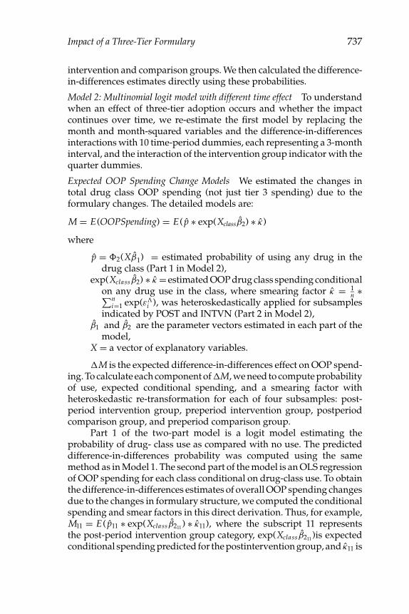
Model 2: Multinomial logit model with different time effect To understandwhen an effect of three-tier adoption occurs and whether the impactcontinues over time, we re-estimate the first model by replacing themonth and month-squared variables and the difference-in-differencesinteractions with 10 time-period dummies, each representing a 3-monthinterval, and the interaction of the intervention group indicator with thequarter dummies.

Expected OOP Spending Change Models We estimated the changes intotal drug class OOP spending (not just tier 3 spending) due to theformulary changes. The detailed models are:

M = E(OOPSpending) = E( p̂ ∗ exp(Xclassβ̂2) ∗ κ̂)

where

p̂ = �2(Xβ̂1) = estimated probability of using any drug in thedrug class (Part 1 in Model 2),

exp(Xclass β̂2) ∗ κ̂ = estimated OOP drug class spending conditionalon any drug use in the class, where smearing factor κ̂ = 1

n ∗∑ni=1 exp(ε�

i ), was heteroskedastically applied for subsamplesindicated by POST and INTVN (Part 2 in Model 2),

β̂1 and β̂2 are the parameter vectors estimated in each part of themodel,

X = a vector of explanatory variables.

�M is the expected difference-in-differences effect on OOP spend-ing. To calculate each component of�M, we need to compute probabilityof use, expected conditional spending, and a smearing factor withheteroskedastic re-transformation for each of four subsamples: post-period intervention group, preperiod intervention group, postperiodcomparison group, and preperiod comparison group.

Part 1 of the two-part model is a logit model estimating theprobability of drug- class use as compared with no use. The predicteddifference-in-differences probability was computed using the samemethod as in Model 1. The second part of the model is an OLS regressionof OOP spending for each class conditional on drug-class use. To obtainthe difference-in-differences estimates of overall OOP spending changesdue to the changes in formulary structure, we computed the conditionalspending and smear factors in this direct derivation. Thus, for example,M11 = E( p̂11 ∗ exp(Xclass β̂211 ) ∗ κ̂11), where the subscript 11 representsthe post-period intervention group category, exp(Xclass β̂211 )is expectedconditional spending predicted for the postintervention group, and κ̂11 is


the smearing factor with heteroskedastic retransformation for the samegroup.

In the OLS models of spending conditional on use, we first useda log transformation of expenditures to alleviate the highly skeweddependent variable. Following the algorithm specified by Manning andMullahy (2001), we first estimated an OLS model for ln(y) = xd+ε andcalculated the log-scale residuals (Manning and Mullahy, 2001). Thelog-scale OLS residuals indicate heteroskedasticity for predicted logspending, the pre-post intervention dummy variable, the interventiongroup indicator, and all other covariates except age between 40–45 and50–55. Due to heteroskedasticity, the OLS method without retransfor-mation will cause biased estimation. The normality test for log-scaleOLS residual notes leptokurtotic residuals (kurtosis = 4.8 and skewness= 0.64), which indicates the distribution of the log-scale residual is nothighly skewed but heavily tailed. Because the leptokurtotic residualswill result in a substantial inefficiency loss from using GLM methods, weselected a robust OLS model with cluster correction and heteroskedasticretransformation.

We discovered the log-scale OLS residual is heteroskedastic tothe predicted dependent variable, so instead of retransforming foreach explanatory variable, we chose to run a nonparametric smearingestimate. First, we computed the exponential of the log-scale residual(call it “smr”) after estimating OLS for ln(y) = xd+ε, and then weran a robust OLS regression with cluster correction of smr on all theright-hand variables as in the original models. Then we computed thepredicted smr values for each subsample: precomparison, postcom-parison, preintervention, and postintervention, which are consideredas smearing factors for each subsample. (Duan et al., 1983; Manning,1998).

Because smearing with heteroskedastic retransformation correctspotential bias caused by the OLS method for the heavy-tailed log-scaleresidual but does not address the imprecision problem, we bootstrapped(1,000 repetitions) to assess the magnitude of the problem. We assessedthe biases and revised confidence intervals for 1,000 repetitions. Becausethe biases of coefficients were very small in comparison to the observedvalues and were too small to affect the confidence interval, we usedrobust OLS estimation for log-transformed expenditures.

5. Results

Descriptive statistics on the study population are found in Table II. Thereare small differences in the demographic characteristics studied betweenthe intervention and comparison groups.


Table II.

Descriptive Statistics for the Study Population

Characteristic Three-tier Group Comparison Group P-value

Age as of 12/31/01 37.51 34.82 <0.05(17.59) (17.14)

% Male 0.47 0.47 NSEmployee Status

% Employee 52.1% 47.5% <0.05% Spouse 20.2% 22.2% <0.05% Dependent 28.0% 31.0% <0.05

Mean Total Spending AcrossUsers

Ace Inhibitors 30.00 29.20 <0.05(16.64) (18.17)

PPIs 119.06 116.87 <0.05(48.68) (43.99)

Statins 76.52 76.29 0.52(34.44) (35.67)

Monthly Probability of UseACE inhibitors 2.3% 2.2% NSPPIs 2.0% 2.0% NSStatins 3.0% 2.9% NS

Total N 11,653 27,051 −

Note: Standard deviations appear in parentheses.

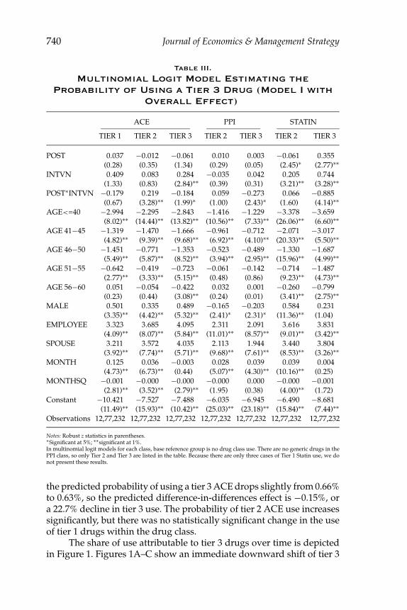
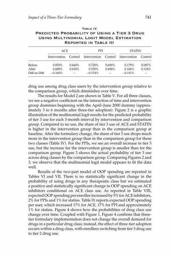
Tables III and IV present results from the Model 1 multinomiallogit model estimating the probability of tier 3 use. The referencecategory is no drug use in each class. For the class of PPIs, there areno results for the probability of selecting tier 1 because there were nogeneric options in this class during the study period. Because only threeenrollees used a generic statin drug, we do not present results for theprobability of selecting a tier 1 statin. For all three classes, we estimatea statistically significant decrease in the likelihood of using a tier 3 drugafter formulary implementation for the intervention group relative tothe comparison group.

As noted above, the expected difference-in-differences effect forthe probability of tier 3 use was constructed using fitted probabilitiesresulting from the multinomial logit model. The unit of observation wasthe person-month. To assess the magnitude of the response we presentresults on the ACE inhibitor class as an example. Before the formularychanges, the sample average of the predicted probability of using a tier 3ACE inhibitor for the intervention group was 0.87%. After the changes,only 0.68% used tier 3 ACE drugs on average. In the comparison group,


Table III.

Multinomial Logit Model Estimating theProbability of Using a Tier 3 Drug (Model I with

Overall Effect)

ACE PPI STATIN

TIER 1 TIER 2 TIER 3 TIER 2 TIER 3 TIER 2 TIER 3

POST 0.037 −0.012 −0.061 0.010 0.003 −0.061 0.355(0.28) (0.35) (1.34) (0.29) (0.05) (2.45)∗ (2.77)∗∗

INTVN 0.409 0.083 0.284 −0.035 0.042 0.205 0.744(1.33) (0.83) (2.84)∗∗ (0.39) (0.31) (3.21)∗∗ (3.28)∗∗

POST∗INTVN −0.179 0.219 −0.184 0.059 −0.273 0.066 −0.885(0.67) (3.28)∗∗ (1.99)∗ (1.00) (2.43)∗ (1.60) (4.14)∗∗

AGE<=40 −2.994 −2.295 −2.843 −1.416 −1.229 −3.378 −3.659(8.02)∗∗ (14.44)∗∗ (13.82)∗∗ (10.56)∗∗ (7.33)∗∗ (26.06)∗∗ (6.60)∗∗

AGE 41−45 −1.319 −1.470 −1.666 −0.961 −0.712 −2.071 −3.017(4.82)∗∗ (9.39)∗∗ (9.68)∗∗ (6.92)∗∗ (4.10)∗∗ (20.33)∗∗ (5.50)∗∗

AGE 46−50 −1.451 −0.771 −1.353 −0.523 −0.489 −1.330 −1.687(5.49)∗∗ (5.87)∗∗ (8.52)∗∗ (3.94)∗∗ (2.95)∗∗ (15.96)∗∗ (4.99)∗∗

AGE 51−55 −0.642 −0.419 −0.723 −0.061 −0.142 −0.714 −1.487(2.77)∗∗ (3.33)∗∗ (5.15)∗∗ (0.48) (0.86) (9.23)∗∗ (4.73)∗∗

AGE 56−60 0.051 −0.054 −0.422 0.032 0.001 −0.260 −0.799(0.23) (0.44) (3.08)∗∗ (0.24) (0.01) (3.41)∗∗ (2.75)∗∗

MALE 0.501 0.335 0.489 −0.165 −0.203 0.584 0.231(3.35)∗∗ (4.42)∗∗ (5.32)∗∗ (2.41)∗ (2.31)∗ (11.36)∗∗ (1.04)

EMPLOYEE 3.323 3.685 4.095 2.311 2.091 3.616 3.831(4.09)∗∗ (8.07)∗∗ (5.84)∗∗ (11.01)∗∗ (8.57)∗∗ (9.01)∗∗ (3.42)∗∗

SPOUSE 3.211 3.572 4.035 2.113 1.944 3.440 3.804(3.92)∗∗ (7.74)∗∗ (5.71)∗∗ (9.68)∗∗ (7.61)∗∗ (8.53)∗∗ (3.26)∗∗

MONTH 0.125 0.036 −0.003 0.028 0.039 0.039 0.004(4.73)∗∗ (6.73)∗∗ (0.44) (5.07)∗∗ (4.30)∗∗ (10.16)∗∗ (0.25)

MONTHSQ −0.001 −0.000 −0.000 −0.000 0.000 −0.000 −0.001(2.81)∗∗ (3.52)∗∗ (2.79)∗∗ (1.95) (0.38) (4.00)∗∗ (1.72)

Constant −10.421 −7.527 −7.488 −6.035 −6.945 −6.490 −8.681(11.49)∗∗ (15.93)∗∗ (10.42)∗∗ (25.03)∗∗ (23.18)∗∗ (15.84)∗∗ (7.44)∗∗

Observations 12,77,232 12,77,232 12,77,232 12,77,232 12,77,232 12,77,232 12,77,232

Notes: Robust z statistics in parentheses.∗Significant at 5%; ∗∗significant at 1%.In multinomial logit models for each class, base reference group is no drug class use. There are no generic drugs in thePPI class, so only Tier 2 and Tier 3 are listed in the table. Because there are only three cases of Tier 1 Statin use, we donot present these results.

the predicted probability of using a tier 3 ACE drops slightly from 0.66%to 0.63%, so the predicted difference-in-differences effect is −0.15%, ora 22.7% decline in tier 3 use. The probability of tier 2 ACE use increasessignificantly, but there was no statistically significant change in the useof tier 1 drugs within the drug class.

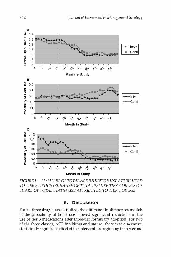
The share of use attributable to tier 3 drugs over time is depictedin Figure 1. Figures 1A–C show an immediate downward shift of tier 3


Table IV.

Predicted Probability of Using a Tier 3 DrugUsing Multinomial Logit Model Estimation

Reported in Table III

ACE PPI STATIN

Intervention Control Intervention Control Intervention Control

Before 0.870% 0.660% 0.720% 0.690% 0.179% 0.087%After 0.680% 0.630% 0.550% 0.694% 0.106% 0.124%Diff-in-Diff −0.160% − −0.174% − −0.111% −

drug use among drug class users by the intervention group relative tothe comparison group, which diminishes over time.

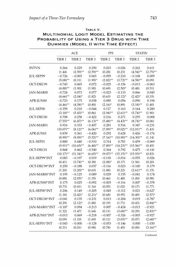
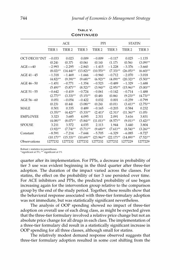
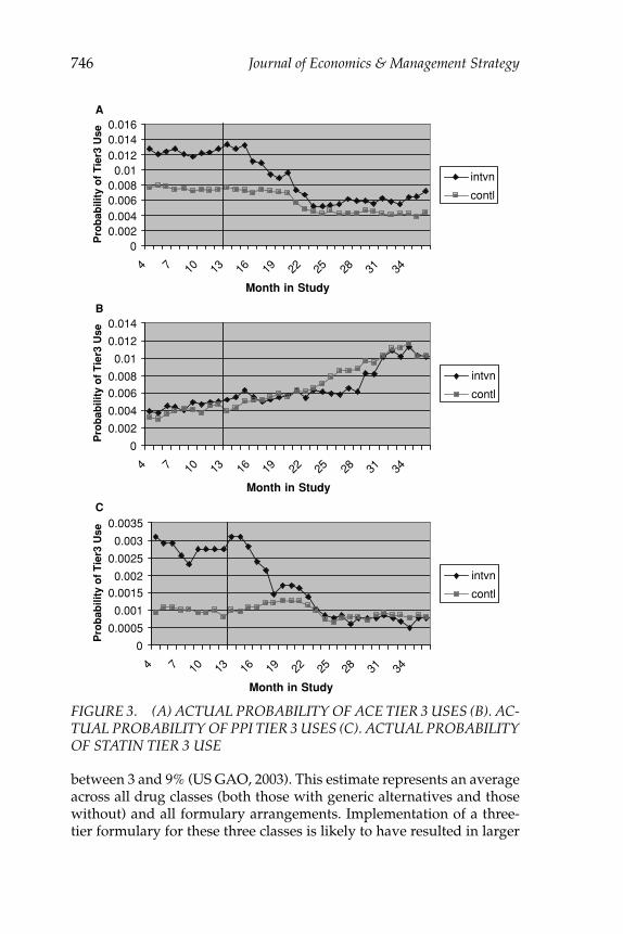
The results for Model 2 are shown in Table V. For all three classes,we see a negative coefficient on the interaction of time and interventiongroup dummies beginning with the April–June 2000 dummy (approx-imately 3 to 6 months after three-tier adoption). Figure 2 is a graphicillustration of the multinomial logit results for the predicted probabilityof tier 3 use for each 3-month interval by intervention and comparisongroup. Compared to no use, the share of tier 3 use of ACE and STATINis higher in the intervention group than in the comparison group atbaseline. After the formulary change, the share of tier 3 use drops muchmore in the intervention group than in the comparison group for thesetwo classes (Table IV). For the PPIs, we see an overall increase in tier 3use, but the increase for the intervention group is smaller than for thecomparison group. Figure 3 shows the actual probability of tier 3 useacross drug classes by the comparison group. Comparing Figures 2 and3, we observe that the multinomial logit model appears to fit the datawell.

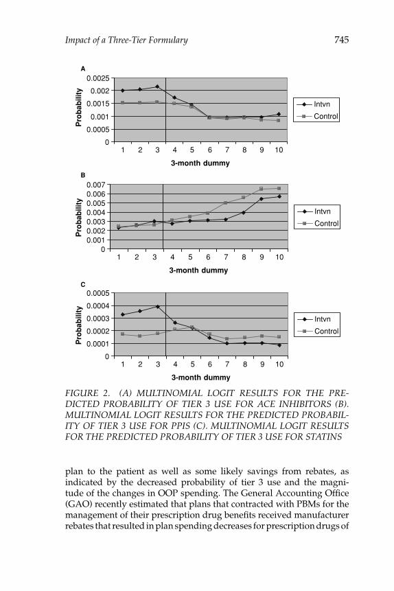
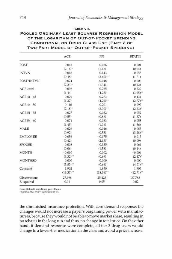
Results of the two-part model of OOP spending are reported inTables VI and VII. There is no statistically significant change in theprobability of using drugs in any therapeutic class but we estimateda positive and statistically significant change in OOP spending on ACEinhibitors conditional on ACE class use. As reported in Table VIII,expected OOP spending per enrollee increased by 5% for ACE inhibitors,2% for PPIs and 1% for statins. Table IX reports expected OOP spendingper user, which increased 17% for ACE, 17% for PPI and approximately1% for statins. Figure 4 shows how the probabilities of drug class usechange over time. Coupled with Figure 1, Figure 4 confirms that three-tier formulary implementation does not change the overall demand fordrugs in a particular drug class; instead, the effect of three-tier adoptionoccurs within a drug class, with enrollees switching from tier 3 drug useto tier 2 drug use.


0

0.1

0.2

0.3

0.4

0.5

0.6

4 7 10 13 16 19 22 25 28 31 34

Month in Study

Pro

bab

ility

of

Tie

r3 U

se

Intvn

Contl

0

0.1

0.2

0.3

0.4

0.5

4 7 10 13 16 19 22 25 28 31 34

Month in Study

Pro

bab

ility

of

Tie

r3 U

se

Intvn

Contl

0

0.02

0.04

0.06

0.08

0.1

0.12

4 7 10 13 16 19 22 25 28 31 34

Month in Study

Pro

bab

ility

of

Tie

r3 U

se

Intvn

Contl

A

B

C

FIGURE 1. (A) SHARE OF TOTAL ACE INHIBITOR USE ATTRIBUTEDTO TIER 3 DRUGS (B). SHARE OF TOTAL PPI USE TIER 3 DRUGS (C).SHARE OF TOTAL STATIN USE ATTRIBUTED TO TIER 3 DRUGS

6. Discussion

For all three drug classes studied, the difference-in-differences modelsof the probability of tier 3 use showed significant reductions in theuse of tier 3 medications after three-tier formulary adoption. For twoof the three classes, ACE inhibitors and statins, there was a negative,statistically significant effect of the intervention beginning in the second


Table V.

Multinomial Logit Model Estimating theProbability of Using a Tier 3 Drug with Time

Dummies (Model II with Time Effect)

ACE PPI STATIN


INTVN 0.266 0.229 0.250 0.023 −0.026 0.262 0.611(1.44) (2.59)∗∗ (2.59)∗∗ (0.28) (0.23) (4.54)∗∗ (2.75)∗∗

JUL-SEP99 −0.726 −0.003 0.065 −0.095 −0.210 −0.108 0.009(5.08)∗∗ (0.11) (1.99)∗ (2.82)∗∗ (3.72)∗∗ (4.58)∗∗ (0.09)

OCT-DEC99 −0.743 0.065 0.072 −0.025 −0.156 −0.013 −0.063(4.88)∗∗ (1.90) (1.90) (0.69) (2.50)∗ (0.48) (0.51)

JAN-MAR00 −0.724 0.073 0.077 −0.023 −0.133 0.066 0.045(4.66)∗∗ (2.04)∗ (1.82) (0.63) (2.12)∗ (2.42)∗ (0.33)

APR-JUN00 −0.723 0.175 0.038 0.085 0.056 0.090 0.194(4.46)∗∗ (4.58)∗∗ (0.80) (2.16)∗ (0.89) (3.18)∗∗ (1.40)

JUL-SEP00 −0.359 0.210 −0.044 0.117 0.163 0.164 0.280(3.18)∗∗ (5.43)∗∗ (0.86) (2.94)∗∗ (2.61)∗∗ (5.74)∗∗ (1.90)

OCT-DEC00 0.708 0.258 −0.422 0.216 0.271 0.255 0.008(7.55)∗∗ (6.47)∗∗ (6.13)∗∗ (5.48)∗∗ (4.43)∗∗ (8.74)∗∗ (0.06)

JAN-MAR01 0.916 0.333 −0.457 0.281 0.516 0.347 −0.231(10.07)∗∗ (8.12)∗∗ (6.06)∗∗ (7.09)∗∗ (9.02)∗∗ (12.01)∗∗ (1.43)

APR-JUN01 0.839 0.361 −0.420 0.292 0.628 0.426 −0.176(8.99)∗∗ (9.09)∗∗ (5.52)∗∗ (7.16)∗∗ (10.90)∗∗ (14.30)∗∗ (1.14)

JUL-SEP01 0.880 0.440 −0.510 0.314 0.781 0.459 −0.069(9.91)∗∗ (10.65)∗∗ (6.48)∗∗ (7.89)∗∗ (14.23)∗∗ (15.56)∗∗ (0.45)

OCT-DEC01 0.868 0.462 −0.540 0.364 0.792 0.475 −0.141(10.17)∗∗ (11.34)∗∗ (6.65)∗∗ (9.07)∗∗ (15.15)∗∗ (15.93)∗∗ (0.83)

JUL-SEP99∗INT 0.083 −0.197 0.019 −0.118 −0.016 −0.055 0.026(0.41) (3.74)∗∗ (0.38) (2.08)∗ (0.17) (1.56) (0.20)

OCT-DEC99∗INT 0.250 −0.188 0.037 −0.116 0.023 −0.100 0.179(1.20) (3.20)∗∗ (0.63) (1.88) (0.22) (2.61)∗∗ (1.15)

JAN-MAR00∗INT 0.195 −0.125 0.089 0.029 0.155 −0.041 0.174(0.88) (2.05)∗ (1.35) (0.46) (1.48) (1.00) (0.98)

APR-JUN00∗INT 0.175 0.025 −0.092 −0.003 −0.116 0.007 −0.378(0.73) (0.41) (1.16) (0.05) (1.02) (0.17) (1.77)

JUL-SEP00∗INT 0.206 0.149 −0.205 0.045 −0.112 0.021 −0.627(1.18) (2.42)∗ (2.21)∗ (0.68) (0.95) (0.49) (2.57)∗

OCT-DEC00∗INT −0.041 0.135 −0.231 0.013 −0.204 0.019 −0.787(0.29) (2.12)∗ (1.88) (0.19) (1.71) (0.43) (2.84)∗∗

JAN-MAR01∗INT −0.187 0.094 −0.213 0.007 −0.424 −0.013 −0.921(1.32) (1.47) (1.64) (0.11) (3.68)∗∗ (0.29) (2.83)∗∗

APR-JUN01∗INT −0.013 0.069 −0.218 −0.007 −0.326 −0.003 −0.927(0.09) (1.10) (1.69) (0.11) (3.03)∗∗ (0.07) (2.68)∗∗

JUL-SEP01∗INT −0.043 −0.000 −0.128 −0.053 −0.146 0.000 −1.030(0.31) (0.01) (0.98) (0.78) (1.45) (0.00) (3.16)∗∗

Continued


Table V.

Continued

ACE PPI STATIN


OCT-DEC01∗INT −0.033 0.023 0.009 −0.009 −0.117 0.025 −1.135(0.24) (0.37) (0.06) (0.14) (1.17) (0.56) (3.09)∗∗

AGE<=40 −2.993 −2.295 −2.843 −1.415 −1.228 −3.376 −3.660(8.02)∗∗ (14.44)∗∗ (13.82)∗∗ (10.55)∗∗ (7.33)∗∗ (26.05)∗∗ (6.60)∗∗

AGE 41−45 −1.318 −1.469 −1.666 −0.960 −0.712 −2.070 −3.018(4.82)∗∗ (9.39)∗∗ (9.68)∗∗ (6.92)∗∗ (4.09)∗∗ (20.32)∗∗ (5.50)∗∗

AGE 46−50 −1.451 −0.771 −1.354 −0.523 −0.489 −1.329 −1.688(5.49)∗∗ (5.87)∗∗ (8.52)∗∗ (3.94)∗∗ (2.95)∗∗ (15.96)∗∗ (5.00)∗∗

AGE 51−55 −0.642 −0.419 −0.724 −0.061 −0.142 −0.714 −1.488(2.77)∗∗ (3.33)∗∗ (5.15)∗∗ (0.48) (0.86) (9.23)∗∗ (4.73)∗∗

AGE 56−60 0.051 −0.054 −0.422 0.032 0.001 −0.259 −0.799(0.23) (0.44) (3.08)∗∗ (0.24) (0.01) (3.41)∗∗ (2.75)∗∗

MALE 0.501 0.335 0.489 −0.165 −0.203 0.584 0.232(3.35)∗∗ (4.42)∗∗ (5.33)∗∗ (2.41)∗ (2.31)∗ (11.36)∗∗ (1.05)

EMPLOYEE 3.323 3.685 4.095 2.311 2.091 3.616 3.831(4.08)∗∗ (8.07)∗∗ (5.84)∗∗ (11.01)∗∗ (8.57)∗∗ (9.01)∗∗ (3.42)∗∗

SPOUSE 3.211 3.572 4.035 2.113 1.944 3.440 3.804(3.92)∗∗ (7.74)∗∗ (5.71)∗∗ (9.68)∗∗ (7.61)∗∗ (8.54)∗∗ (3.26)∗∗

Constant −8.591 −7.214 −7.644 −5.705 −6.329 −6.085 −8.727(10.17)∗∗ (15.33)∗∗ (10.69)∗∗ (23.96)∗∗ (22.17)∗∗ (14.89)∗∗ (7.52)∗∗

Observations 1277232 1277232 1277232 1277232 1277232 1277229 1277229

Robust z statistics in parentheses.∗significant at 5%; ∗∗ significant at 1%

quarter after its implementation. For PPIs, a decrease in probability oftier 3 use was evident beginning in the third quarter after three-tieradoption. The duration of the impact varied across the classes. Forstatins, the effect on the probability of tier 3 use persisted over time.For ACE inhibitors and PPIs, the predicted probability of use beganincreasing again for the intervention group relative to the comparisongroup by the end of the study period. Together, these results show thatthe behavioral response associated with three-tier formulary adoptionwas not immediate, but was statistically significant nevertheless.

The analysis of OOP spending showed no impact of three-tieradoption on overall use of each drug class, as might be expected giventhat the three-tier formulary involved a relative price change but not anabsolute price change for all drugs in each class. The implementation ofa three-tier formulary did result in a statistically significant increase inOOP spending for all three classes, although small for statins.

The relatively modest demand response observed suggests thatthree-tier formulary adoption resulted in some cost shifting from the


0

0.0005

0.001

0.0015

0.002

0.0025

1 2 3 4 5 6 7 8 9 10

3-month dummy

Pro

bab

ility

Intvn

Control

00.0010.0020.0030.0040.0050.0060.007

1 2 3 4 5 6 7 8 9 10

3-month dummy

Pro

bab

ility

Intvn

Control

0

0.0001

0.0002

0.0003

0.0004

0.0005

1 2 3 4 5 6 7 8 9 10

3-month dummy

Pro

bab

ility

Intvn

Control

A

B

C

FIGURE 2. (A) MULTINOMIAL LOGIT RESULTS FOR THE PRE-DICTED PROBABILITY OF TIER 3 USE FOR ACE INHIBITORS (B).MULTINOMIAL LOGIT RESULTS FOR THE PREDICTED PROBABIL-ITY OF TIER 3 USE FOR PPIS (C). MULTINOMIAL LOGIT RESULTSFOR THE PREDICTED PROBABILITY OF TIER 3 USE FOR STATINS

plan to the patient as well as some likely savings from rebates, asindicated by the decreased probability of tier 3 use and the magni-tude of the changes in OOP spending. The General Accounting Office(GAO) recently estimated that plans that contracted with PBMs for themanagement of their prescription drug benefits received manufacturerrebates that resulted in plan spending decreases for prescription drugs of


00.0020.0040.0060.0080.01

0.0120.0140.016

4 7 10 13 16 19 22 25 28 31 34

Month in Study

Pro

bab

ility

of

Tie

r3 U

se

intvn

contl

0

0.002

0.004

0.006

0.008

0.01

0.012

0.014

4 7 10 13 16 19 22 25 28 31 34

Month in Study

Pro

bab

ility

of

Tie

r3 U

se

intvn

contl

0

0.0005

0.001

0.0015

0.002

0.0025

0.003

0.0035

4 7 10 13 16 19 22 25 28 31 34

Month in Study

Pro

bab

ility

of

Tie

r3 U

se

intvn

contl

A

B

C

FIGURE 3. (A) ACTUAL PROBABILITY OF ACE TIER 3 USES (B). AC-TUAL PROBABILITY OF PPI TIER 3 USES (C). ACTUAL PROBABILITYOF STATIN TIER 3 USE

between 3 and 9% (US GAO, 2003). This estimate represents an averageacross all drug classes (both those with generic alternatives and thosewithout) and all formulary arrangements. Implementation of a three-tier formulary for these three classes is likely to have resulted in larger


Table VI.

Logit Model Estimating the Probability of Using aDrug in the Class (Part 1 of Two-Part Model of

Out-of-Pocket Spending)

ACE PPI STATIN

POST −0.027 0.011 −0.040(1.10) (0.38) (1.67)

INTVN 0.195 −0.012 0.243(2.76)∗∗ (0.16) (3.92)∗∗

POST∗INTVN 0.047 −0.050 0.016(1.13) (1.00) (0.40)

AGE<=40 −2.536 −1.352 −3.393(19.85)∗∗ (12.43)∗∗ (26.56)∗∗

AGE 41−45 −1.520 −0.874 −2.109(13.01)∗∗ (7.75)∗∗ (20.98)∗∗

AGE 46−50 −1.020 −0.513 −1.349(9.95)∗∗ (4.76)∗∗ (16.43)∗∗

AGE 51−55 −0.548 −0.087 −0.748(5.69)∗∗ (0.83) (9.80)∗∗

AGE 56−60 −0.164 0.022 −0.286(1.74) (0.20) (3.81)∗∗

MALE 0.400 −0.177 0.570(6.71)∗∗ (3.17)∗∗ (11.23)∗∗

EMPLOYEE 3.750 2.226 3.625(10.07)∗∗ (13.66)∗∗ (9.26)∗∗

SPOUSE 3.655 2.046 3.454(9.73)∗∗ (12.03)∗∗ (8.79)∗∗

MONTH 0.015 0.030 0.035(4.61)∗∗ (6.52)∗∗ (9.78)∗∗

MONTHSQ −0.000 −0.000 −0.000(1.42) (0.87) (3.74)∗∗

Constant −6.676 −5.669 −6.388(17.40)∗∗ (29.62)∗∗ (15.99)∗∗

Observations 1,277,232 1,277,232 1,277,232

Notes: Robust t statistics in parentheses.∗significant at 5%; ∗∗ significant at 1%.

rebates, given the limited generic competition in the classes studiedduring this time period. If so, plan and total savings resulting fromthree-tier formulary adoption may have been of sizeable magnitude.

If demand response for particular drugs within a therapeutic classwere zero, there would be no welfare effects in consumption associatedwith three-tier adoption and the savings to the plan represents a purecost-shift onto enrollees. As a result, a three-tier formulary would serveto remove some risk protection and consumers would lose welfare from


Table VII.

Pooled Ordinary Least Squares Regression Modelof the Logarithm of Out-of-Pocket Spending

Conditional on Drug Class Use (Part 2 ofTwo-Part Model of Out-of-Pocket Spending)

ACE PPI STATIN

POST 0.042 0.026 −0.001(2.16)∗ (1.18) (0.04)

INTVN −0.018 0.143 −0.055(0.48) (3.60)∗∗ (1.71)

POST∗INTVN 0.074 0.048 −0.006(2.23)∗ (1.34) (0.22)

AGE<=40 0.096 0.265 0.229(1.44) (4.28)∗∗ (3.95)∗∗

AGE 41−45 0.079 0.273 0.134(1.37) (4.29)∗∗ (2.77)∗∗

AGE 46−50 0.116 0.201 0.097(2.18)∗ (3.30)∗∗ (2.33)∗

AGE 51−55 0.027 0.052 0.052(0.55) (0.86) (1.37)

AGE 56−60 0.071 0.083 0.055(1.45) (1.36) (1.56)

MALE −0.029 0.016 −0.083(0.92) (0.53) (3.28)∗∗

EMPLOYEE −0.056 −0.175 0.013(0.42) (2.13)∗ (0.09)

SPOUSE −0.008 −0.135 0.064(0.06) (1.58) (0.44)

MONTH −0.010 0.002 −0.006(3.32)∗∗ (0.69) (2.17)∗

MONTHSQ 0.000 0.000 0.000(3.83)∗∗ (0.66) (4.01)∗∗

Constant 1.902 1.950 1.903(13.37)∗∗ (18.36)∗∗ (12.71)∗∗

Observations 27,998 25,423 37,788R-squared 0.01 0.05 0.02

Notes: Robust t statistics in parentheses.∗significant at 5%; ∗∗significant at 1%.

the diminished insurance protection. With zero demand response, thechanges would not increase a payer’s bargaining power with manufac-turers, because they would not be able to move market share, resulting inno rebates in the long run and thus, no change in total price. On the otherhand, if demand response were complete, all tier 3 drug users wouldchange to a lower-tier medication in the class and avoid a price increase.


Table VIII.

Estimated Changes in Expected Out-of-PocketSpending Across All Enrollees

ACE PPI STATIN

Base Out-of-Pocket Spending 1.833 1.825 1.870Expected Out-of-Pocket 0.097 0.030 0.012Spending Change (0.048) (0.014) (0.007)

Percentage Change of Spending 5.29% 1.63% 0.63%

Table IX.

Estimated Change in Expected Out-of-PocketSpending Among Users

ACE PPI STATIN

Base Out-of-Pocket Spending 6.615 8.108 7.00Expected Out-of-Pocket 1.117 1.362 0.0411Spending Change (0.046) (0.156) (0.004)

Percentage Change of Spending 16.89% 16.80% 0.59%

As a result, there would be no change in OOP spending and all gainswould come from savings extracted from pharmaceutical manufacturersin the form of rebates.

Our results fall in between the two polar cases.1 The empiricalestimates of demand response showed notable changes in the demandfor products in response to changes in the OOP price. These rangedfrom 22% to 65% reductions in the probability of using tier 3 drugsin response to the 100% increase in OOP price. This suggests somesignificant behavior change but also cost shifting. The analysis of OOPspending confirms this implication for two of the three classes. Themagnitude of the cost shift was relatively small (17% at most). Weanticipate that the savings obtained by the plans from the ability toredirect demand would likely substantially exceed the cost shift. Thus,the gains to premium payers may well exceed the losses to users ofthe drug classes. It is important to recognize that the results representa single employer’s experience and thus may not reflect the generalexperience.

1. We do not have adequate power to disaggregate impacts of three-tier adoption onnew versus ongoing users of medications for the three classes we studied. Consequently,our results may represent underestimates of demand response if demand of new users ismore sensitive to OOP price than demand of ongoing users.


0.0%0.5%1.0%1.5%2.0%2.5%3.0%3.5%

4 7 10 13 16 19 22 25 28 31 34

Month in Study

IntvnContl

0.0%0.5%1.0%1.5%2.0%2.5%3.0%3.5%4.0%

4 7 10 13 16 19 22 25 28 31 34

Month in Study

IntvnContl

0.0%1.0%

2.0%3.0%4.0%

5.0%6.0%

4 7 10 13 16 19 22 25 28 31 34

Month in Study

IntvnContl

A

B

C

FIGURE 4. (A) PROBABILITY OF ACE INHIBITOR USE OVER TIME(B). PROBABILITY OF PPI USE OVER TIME (C). PROBABILITY OFSTATIN USE OVER TIME

7. Concluding Remarks

In this research we find evidence of moderate demand response to a“pure relative price change” implemented in the context of a three-tier formulary. In our judgment, the savings from increased bargainingpower for plans may well be substantial (since it includes the mostfrequently used drugs in the class). However, we do not have directdata that captures the outcomes of new price negotiations that follow


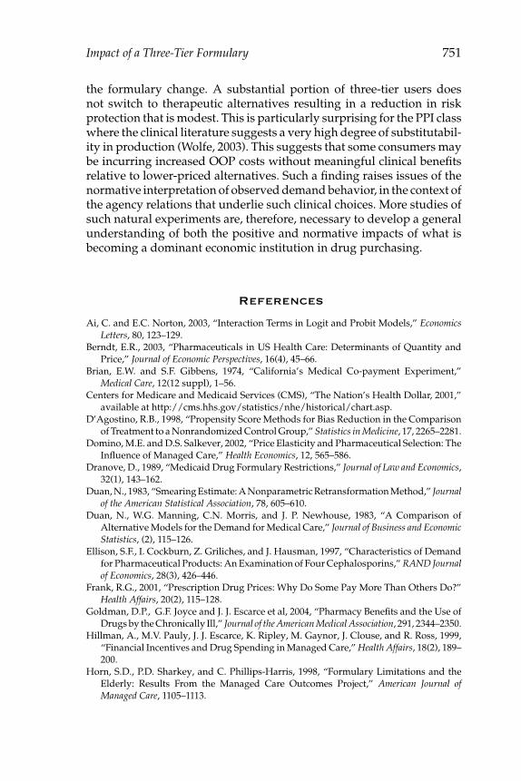
the formulary change. A substantial portion of three-tier users doesnot switch to therapeutic alternatives resulting in a reduction in riskprotection that is modest. This is particularly surprising for the PPI classwhere the clinical literature suggests a very high degree of substitutabil-ity in production (Wolfe, 2003). This suggests that some consumers maybe incurring increased OOP costs without meaningful clinical benefitsrelative to lower-priced alternatives. Such a finding raises issues of thenormative interpretation of observed demand behavior, in the context ofthe agency relations that underlie such clinical choices. More studies ofsuch natural experiments are, therefore, necessary to develop a generalunderstanding of both the positive and normative impacts of what isbecoming a dominant economic institution in drug purchasing.

References

Ai, C. and E.C. Norton, 2003, “Interaction Terms in Logit and Probit Models,” EconomicsLetters, 80, 123–129.

Berndt, E.R., 2003, “Pharmaceuticals in US Health Care: Determinants of Quantity andPrice,” Journal of Economic Perspectives, 16(4), 45–66.

Brian, E.W. and S.F. Gibbens, 1974, “California’s Medical Co-payment Experiment,”Medical Care, 12(12 suppl), 1–56.

Centers for Medicare and Medicaid Services (CMS), “The Nation’s Health Dollar, 2001,”available at http://cms.hhs.gov/statistics/nhe/historical/chart.asp.

D’Agostino, R.B., 1998, “Propensity Score Methods for Bias Reduction in the Comparisonof Treatment to a Nonrandomized Control Group,” Statistics in Medicine, 17, 2265–2281.

Domino, M.E. and D.S. Salkever, 2002, “Price Elasticity and Pharmaceutical Selection: TheInfluence of Managed Care,” Health Economics, 12, 565–586.

Dranove, D., 1989, “Medicaid Drug Formulary Restrictions,” Journal of Law and Economics,32(1), 143–162.

Duan, N., 1983, “Smearing Estimate: A Nonparametric Retransformation Method,” Journalof the American Statistical Association, 78, 605–610.

Duan, N., W.G. Manning, C.N. Morris, and J. P. Newhouse, 1983, “A Comparison ofAlternative Models for the Demand for Medical Care,” Journal of Business and EconomicStatistics, (2), 115–126.

Ellison, S.F., I. Cockburn, Z. Griliches, and J. Hausman, 1997, “Characteristics of Demandfor Pharmaceutical Products: An Examination of Four Cephalosporins,” RAND Journalof Economics, 28(3), 426–446.

Frank, R.G., 2001, “Prescription Drug Prices: Why Do Some Pay More Than Others Do?”Health Affairs, 20(2), 115–128.

Goldman, D.P., G.F. Joyce and J. J. Escarce et al, 2004, “Pharmacy Benefits and the Use ofDrugs by the Chronically Ill,” Journal of the American Medical Association, 291, 2344–2350.

Hillman, A., M.V. Pauly, J. J. Escarce, K. Ripley, M. Gaynor, J. Clouse, and R. Ross, 1999,“Financial Incentives and Drug Spending in Managed Care,” Health Affairs, 18(2), 189–200.

Horn, S.D., P.D. Sharkey, and C. Phillips-Harris, 1998, “Formulary Limitations and theElderly: Results From the Managed Care Outcomes Project,” American Journal ofManaged Care, 1105–1113.


Huber, P.J., 1967, “The Behavior of Maximum Likelihood Estimates under Nonstan-dard Conditions,” In Proceedings of the Fifth Berkeley Symposium on Mathemat-ical Statistics and Probability. Berkeley, CA: University of California Press, 1, 221–233.

Huskamp, H.A., P.A. Deverka, A.M. Epstein, R.S. Epstein, K.A. McGuigan, and R.G. Frank,2003, “The Effect of Incentive-Based Formularies on Prescription-Drug Utilization andSpending,” New England Journal of Medicine, 349, 2224–2232.

——, M.B. Rosenthal, R.G. Frank, and J.P. Newhouse, 2000, “The Medicare PrescriptionDrug Benefit: How Will the Game Be Played,” Health Affairs, 19(2), 8–23.

Kamal-Bahl, S. and B. Briesacher, 2004, “How Do Incentive-based Formularies InfluenceDrug Selection and Spending for Hypertension?” Health Affairs, 23(1), 227–236.

Levy, R. and D. Cocks, 1999, “Component Management Fails to Save Health Care SystemsCosts: The Case of Restrictive Formularies,” second edition, National PharmaceuticalCouncil.

Joyce, G.F., J.J. Escarce, M.D. Solomon, and D.P. Goldman, 2002, “Employer Drug BenefitPlans and Spending on Prescription Drugs,” Journal of the American Medical Association,288(14), 1733–1774.

Kaiser Family Foundation and the Health Research and Educational Trust, 2004, “Em-ployer Health Benefits, 2004 Annual Survey,” http://www.kff.org/insurance/7148/index.cfm [accessed on June 6, 2005].

Kamal-Bahl, S. and B. Briesacher, 2004, “How Do Incentive-based Formularies InfluenceDrug Selection and Spending for Hypertension?” Health Affairs, 23(1), 227–236.

Keeler, E.B. et al, 1986, The Demand for Episodes of Mental Health Services, RAND.Liebowitz, A., W.G. Manning, and J.P. Newhouse, 1985, “The Demand For Prescription

Drugs as a Function of Cost-Sharing,” Social Science and Medicine, 21, 251–277.Ma, C.A. and T.G. McGuire, 2002, “Network Incentives in Managed Health Care,” Journal

of Economics and Management Strategy, II(1), 1–35.Manning, W.G., J.P. Newhouse, N. Duan, E. B. Keeler, A. Leibowitz, and M.S. Marquis,

1987, “Health Insurance and the Demand for Medical Care: Evidence from a Random-ized Experiment,” American Economic Review, 77, 251–277.

——, 1998, “The Logged Dependent Variable, Heteroskedasticity and the Re-transformation Problem,” Journal of Health Economics, 17, 247–281.

Manning, W.G., A. Basu, and J. Mullahy, 2003, “Modeling Costs with Generalized GammaRegression,” working paper.

—— and J. Mullahy, 2001, “Estimating Log Models: To Transform or Not to Transform,”Journal of Health Economics, 20, 461–494, (March 2001).

—— and M.S. Marquis, 1996, “Health Insurance: The Tradeoff Between Risk Pooling andMoral Hazard,” Journal of Health Economics, 15(5), 609–639.

Moore, W.J. and R.J. Newman, 1993, “Drug Formulary Restrictions as a Cost-ContainmentPolicy in Medicaid Programs,” Journal of Law and Economics, XXXVI, 71–97.

Morton, F.S., 1997, “The Strategic Response by Pharmaceutical Firms in the MedicaidMost-Favored-Customer Rules,” RAND Journal of Economics, 28(2), 269–290.

Motheral, B.R. and K.A. Fairman, 2001, “Effect of a Three-Tier Prescription Co-payon Pharmaceutical and Other Medical Utilization,” Medical Care, 39(12), 1293–1304.

Novartis, 2001, Pharmacy Benefit Report: Facts and Figures.Rector, T.S., M.D. Finch, P.M. Danzon, M.V. Pauly, and B. S. Manda, 2003, “Effect of Tiered

Prescription Co-payments on the Use of Preferred Brand Medications,” Medical Care,41(3), 398–406.

Reeder, C. and A. Nelson, 1985, “The Differential Impact of Co-payment on Drug Use ina Medicaid Population,” Inquiry, 22, 396–403.


Rosenthal, M.B., E.R. Berndt, J.M. Donohue, R.G. Frank, and A.M. Epstein, 2002, “Pro-motion of Prescription Drugs to Consumers,” New England Journal of Medicine, 346(7),498–505.

Scherer, F.M., 2000, “The Pharmaceutical Industry,” in Handbook of Health Economics,volume 1B, A.J. Culyer and J.P. Newhouse, eds., New York: Elsevier.

Schweitzer, S.O., 1997, Pharmaceutical Economics and Policy, New York: Oxford UniversityPress.

Sloan, F.A., G.S. Gordon, and D.L. Cocks, 1993, “Hospital-Drug Formularies and Use ofHospital Services,” Medical Care, 31(10), 851–867.

Smith, M. and D. Garner, 1974, “Effects of a Medicaid Program on Prescription-DrugAvailability and Acquisition,” Medical Care, 571–581.

Soumerai, S.B., J. Avorn, D. Ross-Degnan, and S. Gortmaker, 1987, “Payment Restrictionsfor Prescription Drugs under Medicaid: Effects on Therapy, Cost and Equity,” NewEngland Journal of Medicine, 317(9), 550–556.

Tamblyn, R.T., R. Laprise, J.A. Hanley, M. Abrahamowicz, S. Scott, N. Mayo, J. Hurley,R. Grad, E. Latimer, R. Perreault, P. McLeod, A. Huang, P. Larochelle, and L. Mallet,2001, “Adverse Events Associated with Prescription Drug Cost-Sharing among Poorand Elderly Persons,” Journal of the American Medical Association, 285(4), 421–429.

Task Force on Prescription Drugs, US Department of Health, Education and Welfare, 1968,“The Drug Makers and the Drug Distributors,” Washington DC.

Tirole, J., 1992, The Theory of Industrial Organization, Cambridge, Massachusetts: MIT Press.United States General Accounting Office, 2003, Federal Employees’ Health Benefits: Effects of

Using Pharmacy Benefit Managers on Health Plans, Enrollees, and Pharmacies, GAO-03-196,Washington DC: Author.

Viscusi, W.K., J.M. Vernon, and J. E. Harrington, 2000, Economics of Regulation and Antitrust,Cambridge, MA: MIT Press.

White, H., 1980, “A Heteroskedasticity-consistent Covariance Matrix Estimator and aDirect Test for Heteroskedasticity,” Econometrica, 48(4), 817–830.

Wolfe, M.M., 2003, “Overview and Comparison of the Proton-Pump Inhibitors for theTreatment of Acid-related Disorders,” availalable at www.uptodate.com, search on“proton pump inhibitors” [accessed on April 24, 2003].

The Impact of a Three-Tier Formulary on Demand Response for Prescription...

Documents

Transcript of The Impact of a Three-Tier Formulary on Demand Response for Prescription...