The Image Formation Process in Differential Interference ... · PDF fileThe Image Formation...

CARNEGIE MELLONDepartment of Electrical and Computer Engineering~

The Image Formation Process inDifferential Interference Contrast(DIC) Microscopy: A Ray Tracer

Model

Farhana Kagalwala

1996

Advisor: Prof. Kanade

~ gicI

The Image Formation Process in Differential InterferenceContrast (DIC) Microscopy:

A Ray Tracer Model.

By

Farhana Kagalwala

SECTION 1 Introduction 1

SECTION 2 Physics of the DIC Imaging Process

The Electromagnetic Wave Nature of Light 3Amplitude and Phase Objects 5Birefringent Crystals aDIC Microscope Components 7

The Collector and the Condenser 9The Polarizer and the Analyzer 10

Objective Lens and the Imaging System 11

3

SECTION 3 Review of Previous Models for DIC Microscopy

Mathematical Model of Point Spread FunctionAssumptions used 13Derivation of the PSF 13

Signal Processing Approach 15Incorporating Partial Coherence 17Computer Vision Approach 17

12

SECTION 4 Ray Tracer Model for DIC 18

Light Ray Representation 18Representation of the Microscope 19Specimen Model 22Interaction of light rays and matter 23Image Formation Process 26Assumptions and Simplifications 30Software Implementation Details 31

SECTION 5 Simulation Results 34

Etched Glass Test Samples 38Discussion of Results 40

SECTION 6 Conclusion and Future Direction 42

December 17, 1996 i

SECTION 1 Introduction

The Nomarski differential interference contrast (DIC) microscope, the preferred optical system forstudying biological specimens, images variations in the phase of the light wave transmitted through theobserved specimen. Thus it can be used to image objects that are highly transparent in the visible spec-tra and modulate predominantly the phase of the impinging light wave. Within the microscope, theimpinging light wave is split into two wavefronts by a birefringent prism. These wavefronts travel amicroscopic (differential) distance apart through the specimen and finally recombine causing an inter-ference pattern to be detected. In the biological sciences, the DIC microscope is used to examine livespecimens that might be adversely affected by the dyes used in fluorescence imaging. In addition, DICmicroscopy has been shown to have higher resolution along the optical axis than regular phase-contrastmethods, and is therefore a preferred technique for optical sectioning through a specimen under study. 1Optical sectioning is the term used for collecting a series of 2D images, each image is taken with a dif-ferent part of the object brought into focus.

The goal of the current research is to model the image formation process in DIC microscopy. Previouswork dealing with DIC microscopy has formulated analytic models of the image formed by makingstrong assumptions about the specimen and the microscope parameters. This project alms to use amore general technique, specifically ray tracing, to model the intensity distribution at the image planeof the microscope. By using a general object model, the ray-tracer model lifts the assumptionsimposed by earlier works. Simulated images are compared to real microscope data to assess the accu-racy of the ray-tracing approach. The microscope model, and the simulated images, will be used infuture work to reconstruct the actual shape and optical properties of the specimen under study.

1. Ref [2]

Master’s Thesis 1

Introduction

FIGURE 1. DIC image of the nucleus of a fibroblast cell. (Image courtesy of Patricia Feinegle.)

The specimen reconstruction algorithm is intended to contain two parts. The first part will be a simula-tion of the DIC imaging process as presented in the current thesis, and the second part will be a speci-men estimation algorithm.

An added advantage of the ray tracer simulation is that microscope parameters can be modified inter-actively via the user interface and the effect of these parameters on the image can be calculated. Thetranslational position of one of the prisms is one of the microscope parameters. Using a ray-tracer, illu-mination conditions affecting the image quality can be studied. By characterizing the optical propertiesand geometry of objects, one can study how effective DIC microscopy would be to image a particularobject without investing time and resources in the setup of the actual optical components.

2 December 20,1996

The Electromagnetic Wave Nature of Light

SECTION 2 Physics of the DIC Imaging

Process

2.1 The Electromagnetic Wave Nature of Light

An electric field,E, the result of a charge experiencing a vector force FE, is defined by /~E = q’/~

A charge with velocity, v, may experience another force FM, inducing a magnetic field according to the

equation, PM = q~ ×/~ ¯ In addition, according to Faraday’s Induction Law, a time-varying mag-netic field can generate an electric field which is perpendicular to the magnetic field everywhere. Amagnetic field, in turn, is generated by a time-varying electric field. Any simultaneous electric andmagnetic disturbance, satisfying Maxwell’s equations, is called an electromagnetic (EM) wave. electromagnetic wave is described by its direction of propagation, the orientation and magnitude of itselectric field (E-field). Since the magnetic field is everywhere perpendicular to the electric field, with proportional amplitude, it does not have to be separately represented. The propagation direction andthe E-field components can be written as space and time dependent vector functions.

Master’s Thesis 3

Physics of the DIC Imaging Process

direction ofpropagation

i

Y -o~ o X-1 -10

FIGURE 2. Linearly polarized harmonic wave with two orthogonal components (Ez and Ey) of theelectric field amplitude vector (E).

A linearly polarized, harmonic wave propagating along the x axis can be represented by the followingequation,

E(x,t) = EoCOS (w(t + x/c))

where e is the phase of the wave, w is the radian frequency, c is the speed of light in vacuum, and Eo isthe amplitude of the wave. In addition, the electric field component, at any time instant, can be decom-posed into two orthogonal components along selected axes, resulting in the wave represented in figure

2.The spatial period of the wave is denoted by Z, the temporal period is denoted by x, and the angularfrequency by w = 2n/x . Each component, Ey and Ez, can be represented by the above equa-tion.Using the complex representation to simplify mathematical derivations, E can also be defined as

E(x,t) = Re{Eoei(wt + kx + ~)}

where

rated,k = 2n/k. The complex representation allows the spatial and time components to be sepa-

E(x, t) = e-i(kx- e)eiWt = Aiwt, A = Eoe i(kx ~)

4 December 20, 1996

Amplitude and Phase Objects

where A is the complex amplitude, and e/wt is the harmonic time factor. It is assumed that only the realcomponent of the above exponential is of interest, and therefore will not be explicitly denoted in theequation.

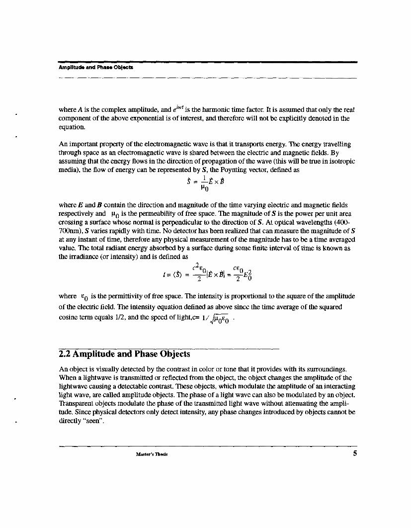
An important property of the electromagnetic wave is that it transports energy. The energy travellingthrough space as an electromagnetic wave is shared between the electric and magnetic fields. Byassuming that the energy flows in the direction of propagation of the wave (this will be true in isotropicmedia), the flow of energy can be represented by S, the Poynting vector, defined as

where E and B contain the direction and magnitude of the time varying electric and magnetic fieldsrespectively and It 0 is the permeability of free space. The magnitude of $ is the power per unit areacrossing a surface whose normal is perpendicular to the direction of S. At optical wavelengths (400-700nm), S varies rapidly with time. No detector has been realized that can measure the magnitude orsat any instant of time, therefore any physical measurement of the magnitude has to be a time averagedvalue. The total radiant energy absorbed by a surface during some finite interval of time is known asthe irradiance (or intensity) and is defined

c2e0 ce0 2I--- <~) = --~---I/~ x/~l = "~’-E0

where e0 is the permittivity of free space. The intensity is proportional to the square of the amplitudeof the electric field. The intensity equation defined as above since the time average of the squared

cosine term equals 1/2, and the speed of light,c= 1/~-~e0 .

2.2 Amplitude and Phase Objects

An object is visually detected by the contrast in color or tone that it provides with its surroundings.When a lightwave is transmitted or reflected from the object, the object changes the amplitude of thelightwave causing a detectable contrast. These objects, which modulate the amplitude of an interactinglight wave, are called amplitude objects. The phase of a light wave can also be modulated by an object.Transparent objects modulate the phase of the transmitted light wave without attenuating the ampli-tude. Since physical detectors only detect intensity, any phase changes introduced by objects cannot bedirectly "seen".

Master’s Thesis 5


Live biological specimens are predominantly phase objects and therefore require techniques whichconvert the phase modulation of a disturbance into an amplitude modulation. Fluorescence microscopyoffers a solution by dyeing the specimens and converting them to amplitude objects, thus making themdetectable. The disadvantage with this method is that the dyes can kill live specimens, and thereforelimiting its use in biological studies. On the other hand, DIC microscopy renders the phase modulatedlight wave detectable by the causing two mutually coherent waves, which have travelled a differentialdistance apart through the phase object, to interfere.

2.3 Birefringent Crystals

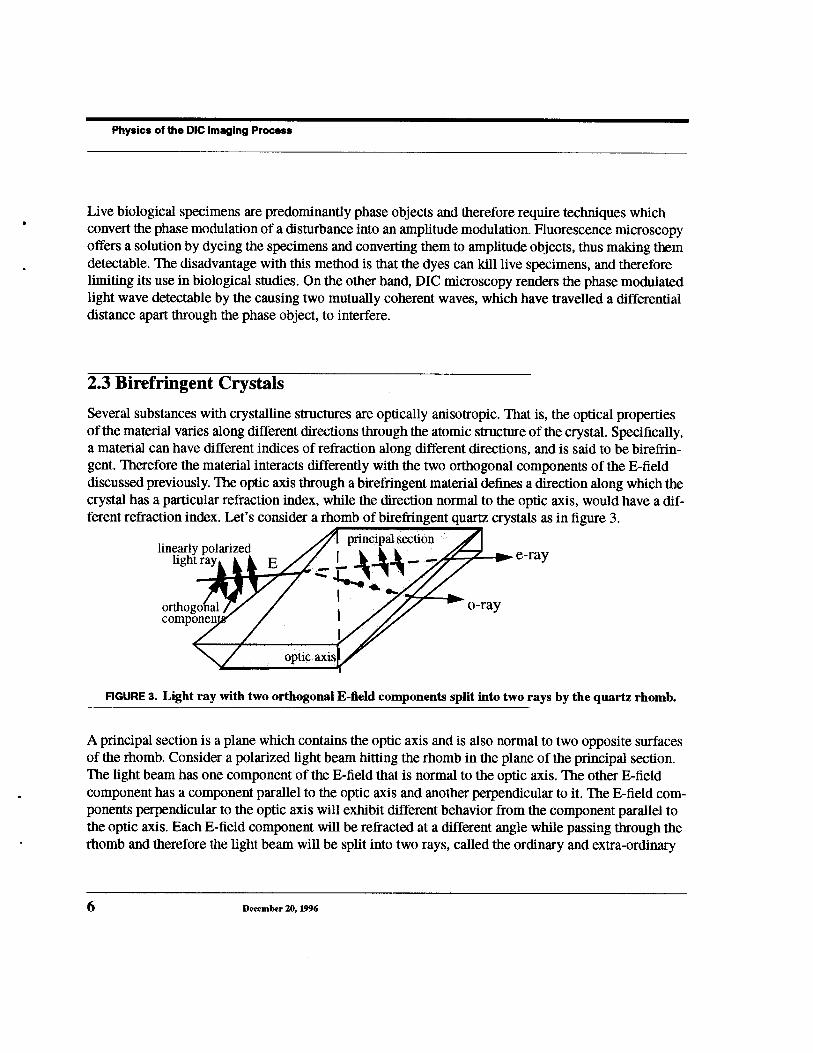
Several substances with crystalline structures are optically anisotropic. That is, the optical propertiesof the material varies along different directions through the atomic structure of the crystal. Specifically,a material can have different indices of refraction along different directions, and is said to be birefrin-gent. Therefore the material interacts differently with the two orthogonal components of the E-fielddiscussed previously. The optic axis through a birefringent material defines a direction along which thecrystal has a particular refraction index, while the direction normal to the optic axis, would have a dif-ferent refraction index. Let’s consider a rhomb of birefringent quartz crystals as in figure 3.

linearly polarized,light ray E e-ray

-- I rorthogo~/~/

opec ~is

FIGURE 3. Light ray with two orthogonai E-field components split into two rays by the quartz rhomb.

A principal section is a plane which contains the optic axis and is also normal to two opposite surfacesof the rhomb. Consider a polarized light beam hitting the rhomb in the plane of the principal section.The light beam has one component of the E-field that is normal to the optic axis. The other E-fieldcomponent has a component parallel to the optic axis and another perpendicular to it. The E-field com-ponents perpendicular to the optic axis will exhibit different behavior from the component parallel tothe optic axis. Each E-field component will be refracted at a different angle while passing through therhomb and therefore the light beam will be split into two rays, called the ordinary and extra-ordinary

6 December 20,1996

DIC Microscope Components

rays. The Wollaston prism used for DIC optics is made of two quartz wedges optically seamed, withthe two optic axes orthogonally aligned. Any linearly polarized light beams entering the prism will besplit into two beams as the different components experience different angles of refraction. It should benoted that different propagation angles through isotropic media represents a linear phase delay.

2.4 DIC Microscope Components

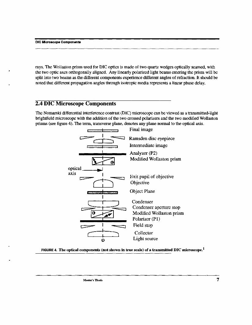
The Nomarski differential interference contrast (DIC) microscope can be viewed as a transmitted-lightbrightfield microscope with the addition of the two crossed polarizers and the two modified Wollastonprisms (see figure 4). The term, transverse plane, denotes any plane normal to the optical axis.

opticalaxis

Final image

Ramsden disc eyepiece

Intermediate image

Analyzer (P2)Modified Wollaston prism

Exit pupil of objectiveObjective

Object Plane

CondenserCondenser aperture stopModified Wollaston prismPolarizer (P1)Field stop

CollectorLight source

FIGURE 4. The optical components (not shown in true scale) of a transmitted DIC microscope.1

Master’s Thesis 7

Physics of the DIC imaging Process

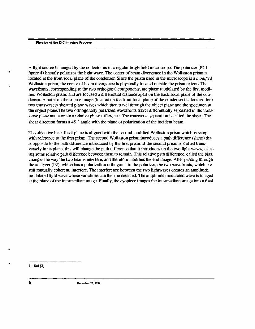
A light source is imaged by the collector as in a regular brightfield microscope. The polarizer (P1 infigure 4) linearly polarizes the light wave. The center of beam divergence in the Wollaston prism islocated at the front focal plane of the condenser. Since the prism used in the microscope is a modifiedWollaston prism, the center of beam divergence is physically located outside the prism extents.Thewavefronts, corresponding to the two orthogonal components, are phase modulated by the first modi-fied Wollaston prism, and are focused a differential distance apart on the back focal plane of the con-denser. A point on the source image (located on the front focal plane of the condenser) is focused intotwo transversely sheared plane waves which then travel through the object plane and the specimen inthe object plane.The two orthogonally polarized wavefronts travel differentially separated in the trans-verse plane and contain a relative phase difference. The transverse separation is called the shear. Theshear direction forms a 45 ° angle with the plane of polarization of the incident beam.

The objective back focal plane is aligned with the second modified Wollaston prism which is setupwith reference to the first prism. The second Wollaston prism introduces a path difference (shear) thatis opposite to the path difference introduced by the first prism. If the second prism is shifted trans-versely in its plane, this will change the path difference that it introduces on the two light waves, caus-ing some relative path difference between them to remain. This relative path difference, called the bias,changes the way the two beams interfere, and therefore modifies the end image. After passing throughthe analyzer (P2), which has a polarization orthogonal to the polarizer, the two wavefronts, which arestill mutually coherent, interfere. The interference between the two lightwaves creates an amplitudemodulated light wave whose variations can then be detected. The amplitude modulated wave is imagedat the plane of the intermediate image. Finally, the eyepiece images the intermediate image into a final

1. Ref [2]

8 December 20, 1996


image that is formed on the retina of the observer. In the case of a camera mounted onto the micro-scope, the intermediate image is imaged onto the array of photodetectors.

condenserfront focal planefield stop ¯ p, ism object

lsi°ghjce ~/~ ~,~~

collectorc~c ndenser

aperture

image plane

Iiobjective

lens & objectiveaperture back focal plane

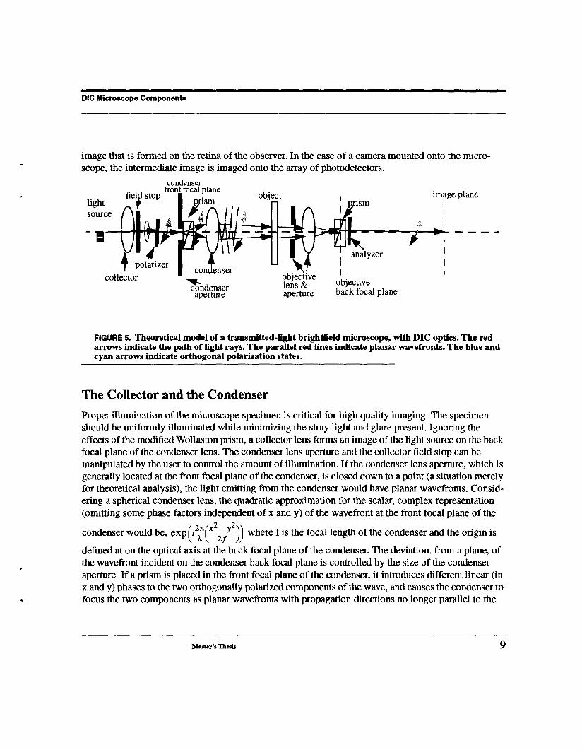
FIGURE S. Theoretical model of a transmitted-light brightfield microscope, with DIC optics. The redarrows indicate the path of light rays. The parallel red lines indicate planar wavefronts. The blue andcyan arrows indicate orthogonal polarization states.

The Collector and the Condenser

Proper illumination of the microscope specimen is critical for high quality imaging. The specimenshould be uniformly illuminated while minimizing the stray light and glare present. Ignoring theeffects of the modified Wollaston prism, a collector lens forms an image of the light source on the backfocal plane of the condenser lens. The condenser lens aperture and the collector field stop can bemanipulated by the user to control the amount of illumination. If the condenser lens aperture, which isgenerally located at the front focal plane of the condenser, is closed down to a point (a situation merelyfor theoretical analysis), the light emitting from the condenser would have planar wavefronts. Consid-ering a spherical condenser lens, the quadratic approximation for the scalar, complex representation(omitting some phase factors independent of x and y) of the wavefront at the front focal plane of the

wou. w ere ,is ,oc len, o, o ,in,sdefined at on the optical axis at the back focal plane of the condenser. The deviation, from a plane, ofthe wavefront incident on the condenser back focal plane is controlled by the size of the condenseraperture. If a prism is placed in the front focal plane of the condenser, it introduces different linear (inx and y) phases to the two orthogonally polarized components of the wave, and causes the condenser tofocus the two components as planar wavefronts with propagation directions no longer parallel to the

Master’s Thesis 9


optical axis. Therefore the approximate complex representation of the one of the wavefronts at the

front focal plane of the condenser would now be exp(i2---~(x2+ax+by+c+ y2))2f , where a, b, and c are

constants. The corresponding wavefront would could be approximated with exp((i2--~(ax+by+c.))) at_ _ __2f

the back focal plane of the condenser.

The Polarizer and the Analyzer

An arbitrary electric field vector can be represented by two orthogonal optical disturbances of theform,

Ex(z, t) = )(Eoxcos(kz-

Ey(Z, t) = }(Eoycos(kz-

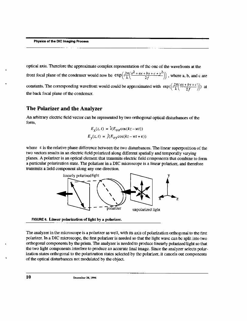
where e is the relative phase difference between the two disturbances. The linear superposition of thetwo vectors results in an electric field polarized along different spatially and temporally varyingplanes. A polarizer is an optical element that transmits electric field components that combine to forma particular polarization state. The polarizer in a DIC microscope is a linear polarizer, and thereforetransmits a field component along any one direction.

~ -- -- -~oTar~zer

unpolarized light

z

FIGURE 6. Linear polarization of light by a polarizer.

The analyzer in the microscope is a polarizer as well, with its axis of polarization orthogonal to the firstpolarizer. In a DIC microscope, the first polarizer is needed so that the light wave can be split into twoorthogonal components by the prism. The analyzer is needed to produce linearly polarized light so thatthe two light components interfere to produce an accurate final image. Since the analyzer selects polar-ization states orthogonal to the polarization states selected by the polarizer, it cancels out componentsof the optical disturbances not modulated by the object.

10 December 20, 1996


Objective Lens and the Imaging System

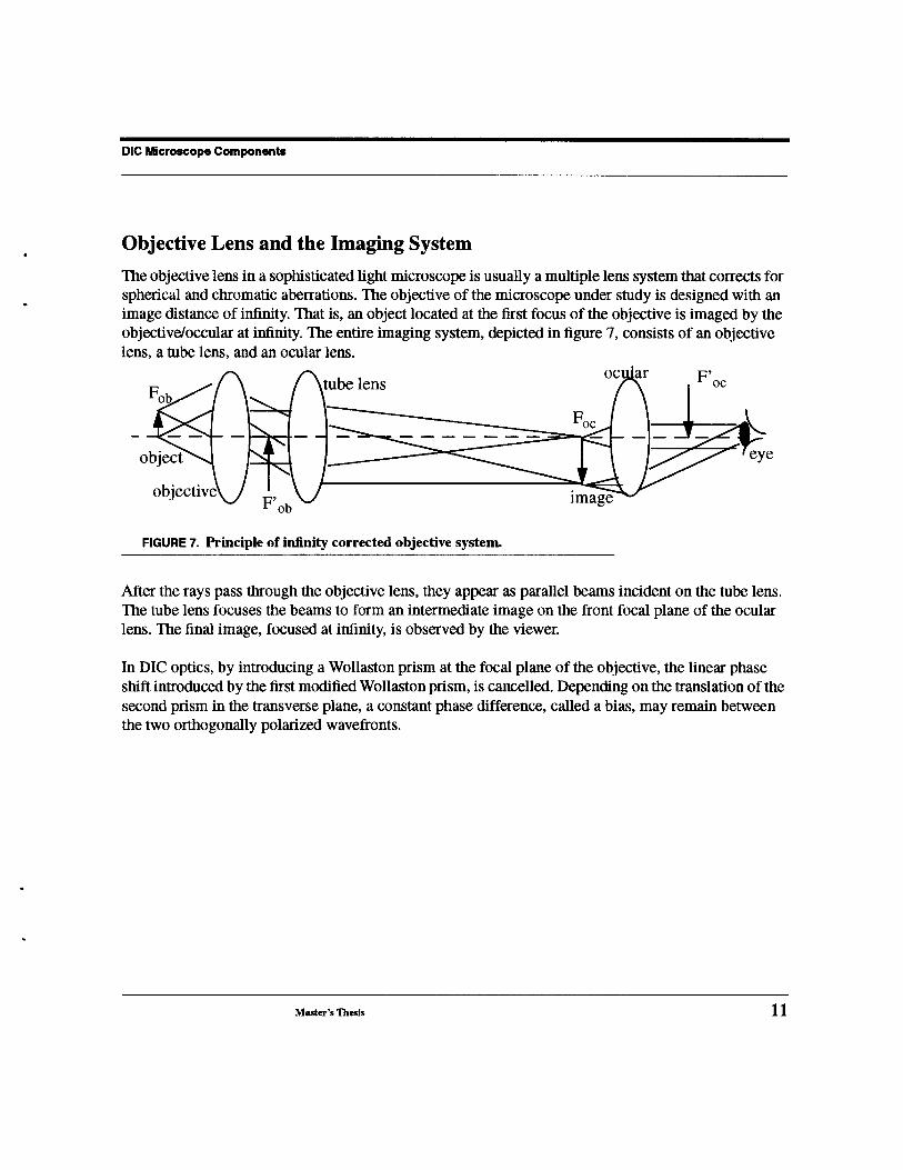
The objective lens in a sophisticated light microscope is usually a multiple lens system that corrects forspherical and chromatic aberrations. The objective of the microscope under study is designed with animage distance of infinity. That is, an object located at the first focus of the objective is imaged by theobjective/occular at infinity. The entire imaging system, depicted in figure 7, consists of an objectivelens, a tube lens, and an ocular lens.

~ 1,. /~tube lens

o~ iF’oc_ Foc I I 1

°bject°bjecti~ve

F,ob~ lllli:t~U -

FIGURE 7. Principle of infinity corrected objective system.

After the rays pass through the objective lens, they appear as parallel beams incident on the tube lens.The tube lens focuses the beams to form an intermediate image on the front focal plane of the ocularlens. The final image, focused at infinity, is observed by the viewer.

In DIC optics, by introducing a Wollaston prism at the focal plane of the objective, the linear phaseshift introduced by the first modified Wollaston prism, is cancelled. Depending on the translation of thesecond prism in the transverse plane, a constant phase difference, called a bias, may remain betweenthe two orthogonally polarized wavefronts.

Master’s Th~is 11

Review of Previous Models for DIC Microscopy

SECTION 3 Review of Previous Models forDIC Microscopy

3.1 Mathematical Model of Point Spread Function

Galbraith1 derived a mathematical point spread function of a DIC microscope using a formulation ofthe point spread function of a standard brighttield transmitted light microscope.His derivation startedwith the Huygens-Fresnel integral and evaluated it in terms of convergent series of Bessel functions tomake it computationally feasible. The Huygens-Fresnel integral expresses the complex amplitude interms of wavelength and geometrical parameters.

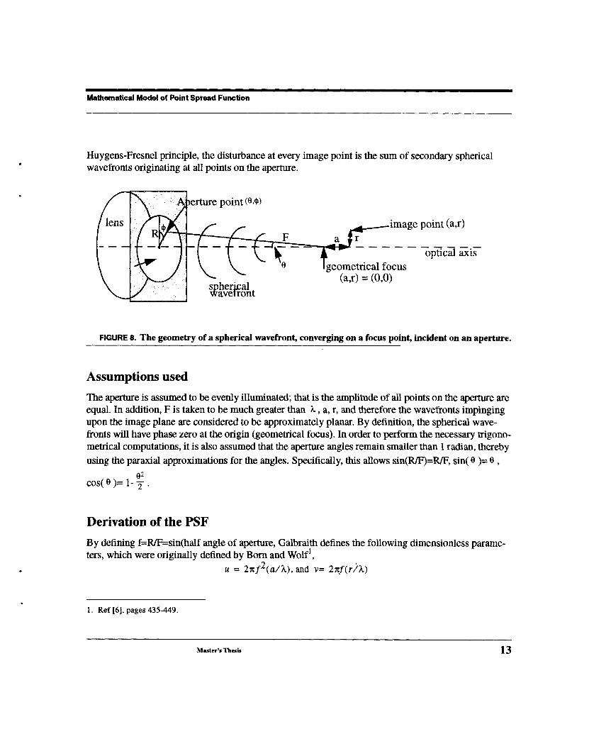
A spherical wavefront, wavelength X, radius E emitted from a circular aperture of radius R is made tofocus at a point by a lens, as depicted in figure 8. The symmetry radially along the optical axis allowsan image point to be specified by its axial displacement (a) from the origin (geometrical focus point)and by its radial distance from the axis (r). In order to determine the nature of the optical disturbance any image point, it is necessary to find its complex amplitude,(K+iL), at each image point (as). Everypoint on the aperture is defined by the aperture angle, o, and the azimuth angle, ~ .According to the

I. Ref [16], Ref [17]


Mathematical Model of Point Spread Function

Huygens-Fresnel principle, the disturbance at every image point is the sum of secondary sphericalwavefronts originating at all points on the aperture.

¯ i A~erture point

ii!q[ /" ~" ~image point (a,r)

~ ~0 Igeometrical focus

soherical(a,r) = (0,0)

wavetront

FIGURE 8. The geometry of a spherical wavefront, converging on a focus point, incident on an aperture.

Assumptions used

The aperture is assumed to be evenly illuminated; that is the amplitude of all points on the aperture areequal. In addition, F is taken to be much greater than ~., a, r, and therefore the wavefronts impingingupon the image plane are considered to be approximately planar. By definition, the spherical wave-fronts will have phase zero at the origin (geometrical focus). In order to perform the necessary trigono-metrical computations, it is also assumed that the aperture angles remain smaller than 1 radian, thereby

using the paraxial approximations for the angles. Specifically, this allows sin(R/F)=R/F, sin( o )=

cos(0)= 1-T.

Derivation of the PSF

By defining f=R/F=sin(half angle of aperture, Galbraith defines the following dimensionless parame-ters, which were originally defined by Born and Wolf1,

u = 2rcf2(a/)~), and v= 2xf(r,)~.)

1. Ref [6], pages 435-449.

Master’s Thesis 13

Review of Previous Models for OIC Microscopy

The path difference,P, to the point (a,r) and the difference between the phases at (a,r) and (0,0) been determined by Galbraith to be,

P = r- sin0. cosO-(a-cos0)

Substituting the equations for u and v, the scalar field E (with Eo=l) can then be defined

E(u, v) = v. sin0. cos¢/f-(u- cos0/f2) .

For an arbitrary aperture angle, the real (K) and imaginary (L) parts of the complex amplitude defined as the contribution from all points on the infinitely thin aperture for any one angle, 0.

K = 2- sin0. ~ (cosE.d¢)

(¢ = 0)

L = 2.sin0. ~ (sinE-de)

(¢ = o)

By substituting the equation for E, rewriting the resulting integrals as Bessel functions, and using thesmall angle assumptions, the following form of K and L, for all aperture angles, can be obtained.

f

2f2)~=0

Galbraith rewrites the equations in terms of a convergent series (see section 4.5) to facilitate computa-tion, but those equations are not re-derived here.

For DIC microscopy, the above complex amplitude has to be modified according to the effects of thetransverse shear, the phase bias between the interfering wavefronts and the amplitude ratio of the twowavefronts. The shear value, S, is expressed in terms of v/x The intensity distribution is sheared into


Signal Processing Approach

two components along the x-axis with centers at (~S/2, 0,0) and (-~S/2, 0,0). The phase bias, ¯, expressed in wavelengths, and the amplitude ratio is denoted by R. Using the development of the com-plex amplitude at a image point as outlined above, Galbralth defines the complex amplitude of the twosheared wavefronts at the image plane as,

L1 = L(u1, Vl). (l-R)

K1 = K(Ul, Vl). (l-R)K2 = K(u2, v2) ̄ R. cos~ - L(u2, v2) ¯ R. sin~,

L2 = L(u2, v2)- R. cos~ - K(u2,v2) ¯ R. sin~

where K(ui,vi) and L(ui,vi) are defined above

uI = z,u2 : z,v1 = ,f(x- ~S/2)2 + y2,v2 = ~(x + ~S/2)2 + y2

3.2 Signal Processing Approach

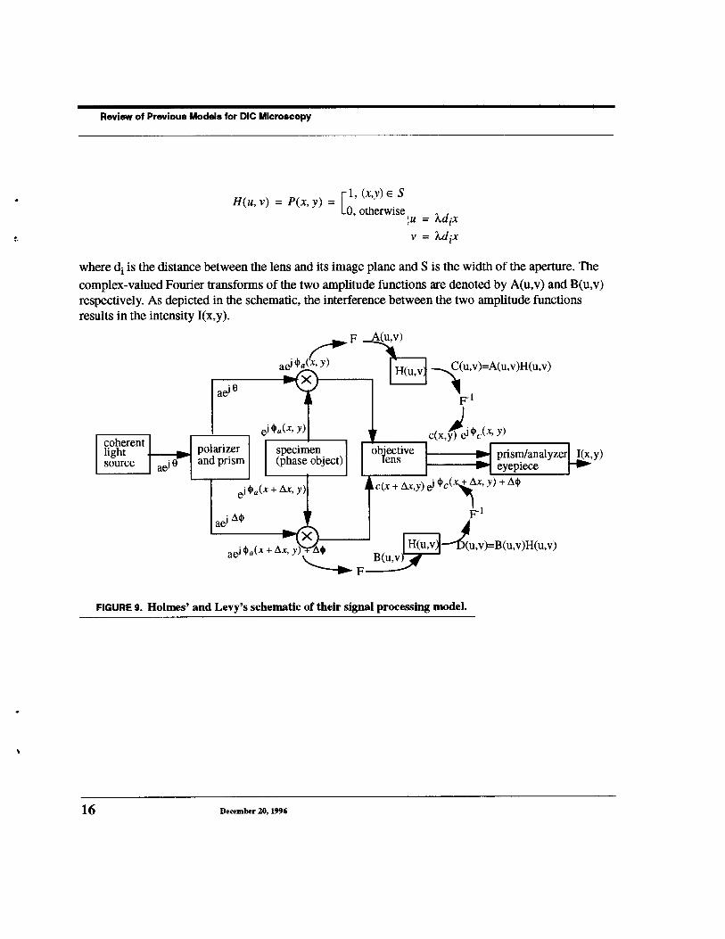
Holmes and Levy1 formulated another model of the DIC image formation process using Fourieroptics. A coherent light source passes through the polarizer/prism/condenser combination to producetwo beams separated by a lateral shift, Ax, and with a phase difference between them, A~. The spec-

imen introduces a spatially varying phase retardation on the first beam, denoted by ¢~a(X, y). The sec-

ond beam also suffers a phase retardation, q~a(X + Ax, y), which is a shifted version of the first beam’sphase delay. Therefore the complex signal of the first beam can be represented by

~(x, y) = a(x, y)exp[jC#a(x, y)]

and the complex signal of the second beam by

[~(x, y) = b(x,y)exp [jCb(X, y)], where Cb = ~a(x + Ax, y) +

The coherent transfer function of the objective lens, H(u,v), is determined by the pupil function of theaperture. Thomas and Levy use a square aperture that has a transmittance 1.0 in the open region and atransmittance of 0 in the opaque region. (In reality, the aperture of the lens is circular.) Therefore,

1. Ref [26]


Review of Previous Models for DIC Microscopy

i1,(x,y) ~ H(u, v) = P(x, y) = 0, otherwise u = ~.dix

v = kdix

where di is the distance between the lens and its image plane and S is the width of the aperture. The

complex-valued Fourier transforms of the two amplitude functions are denoted by A(u,v) and B(u,v)respectively. As depicted in the schematic, the interference between the two amplitude functionsresults in the intensity I(x,y).

aeJ~a ((y~F ~ _~(u,v)=A(u,v)H(u,v)

ae~0 i~ & __~A~_ i F-I

ej ~a c(x,y) e" ~c(x’ y)

~ pol~zerI s~cimen

o~ve --I pfis~an~yz~,y,and prism (phase obj~t) ~ens ~[ eyepiece ~

I O~a(X +~, y~’C(X+ ~,y) O ~C(~~’ Y)+~

aO #~(x + ~x’ Y)~ F B(u’v~~U’v)=B(u’v)H(u’v)

coherentlightsource

FIGURE 9. Holmes’ and Levy’s schematic of their signal processing model.


IncorporaUng Partial Coherence

3.3 Incorporating Partial Coherence

Preza, et al,1 extended the approaches above to incorporate the partial coherence of the illumination.The authors assume a thin (with respect to the illuminating wavelength), highly planar and negligiblydiffracting specimen and monochromatic illumination. They represent the DIC optics as a linear shift-invariant system characterized by the point spread function derived by Galbraith above,. The phase ofthe illumination at the condenser aperture is modeled by a zero-mean, white random process, with aknown covariance, denoted by Uc. The coherence of the illumination is captured in the characteriza-tion of the random process. The complex amplitude of the wave field at the image plane is representedby the following two-dimensional convolution

where Uo(xo,Yo)=f(xo,Yo)Uc(xo,Yo) is the complex amplitude of the wave transmitted by the specimen.The intensity of the image is obtained from the above equation by taking its magnitude squared, andsubstituting the covariance of the wave incident upon the condenser.

3.4 Computer Vision Approach

Patricia Feinegle2 extracted shapes of specimens imaged under DIC optics by assuming that theshadow-cast appearance on the images represented areas where the specimen’s phase transmission var-ied along the shear direction. She used the approach of dynamic contours in computer vision to extractspecimen shapes and to track cell motility. Using forces to attract contours to image edge points rela-tive to the shear direction, she segmented cell structures in DIC images. The deformable snakes algo-rithrn was applied to cell metamorphosis in image sequences to track deformations. In addition, thework also made use of active particles to track cell motility.

1. Ref [35]

2. Ref [14]


Ray Tracer Model for DIC

SECTION 4 Ray Tracer Model for DIC

Using the principles of geometrical optics, a ray tracer simulates the interaction of an impinging lightwavefront with objects modeled in the system. The light wavefront is represented by rays. Each raycan be viewed as the normal to the local planar approximation of the light wavefront. The size of theplanar region is determined by the sampling period of the simulated light wavefront. Since the DICmicroscope images the variations in the phase of the light wave transmitted through the specimen andoptical components, the complete local electric field of the light wave has to be represented in the raytracer. The interaction between each ray and the different components in the microscope has to accountfor the amplitude, polarization, and phase of the electric fidd. In addition, the image formed on theimage plane in the microscope is distorted by diffraction effects. In the present model, a simplifiedeffect of diffraction is used. Due to the narrow spectrum of the illuminating wavefront, the ray-tracermodel contains light rays of only one wavelength, but this can be easily generalized by casting rays ofdifferent wavelengths across the spectrum of the illuminating beam, and modifying the index of refrac-tion of materials according to the ray’s wavelength.

4.1 Light Ray Representation

Each ray vector carries information about a local region in the transmitted fight wave from. A ray vec-tor contains transient characteristics of the electric field, such as position, propagation direction, dis-


Representation of the Microscope

tance travelled, polarization vectors, and phase, in addition to the global characteristics such aswavelength. As discussed in section 2, the electric and magnetic field vectors are perpendicular to thedirection of propagation. The origin of each light ray determines where this ray was "born" and thedistance along the ray determines how far the ray has travelled from the origin in the propagationdirection. The polarization of the E-field amplitude vectors are represented by Jones vectors in thelocal coordinate system of each ray. The local coordinate system at each ray is defined by the propaga-tion direction vector k, and two orthogonal vectors, s and p, in the plane perpendicular to k.

Jones vectors represent the instantaneous scalar components, Ex(t) and Ey(t), of the E-field while serving their relative phase information, where the x,y directions lie in the plane perpendicular to thepropagation vector and are orthogonal. Therefore,

1

represents the polarization state of a coherent wave. For example, a linearly polarized wave at 45 o canbe represented by

EoE =

and a circularly polarized wave is represented by

I Eo i9x

E= I ---~elEo

l"-~e

4.2 Representation of the Microscope

The complete microscope is represented by a spatial grid of objects where each object is a model of anoptical component in the microscope. The world coordinate system used is aligned such that the z axisis the optical axis (therefore the lens’ centers intersect the z axis) and the x-y planes are transverse the optical axis. The objects are separated by distances as dictated by standard microscope configura-



tions and information from the manufacturer. The model deviates from the actual microscope since thecondenser and polarizer are not modeled, and the objective lens model is simplified. In an actualmicroscope, the path between the illumination source and the specimen contains at least two lens sys-tems, each of which might be a multiple lens system, and the polarizer. In order to simplify the imple-mentation of the microscope model, the illuminating beam is assumed to result in a planar wavefrontafter passing through the condenser and polarizer. Light rays originate from sampled points on thesewavefronts.

f~~____~ ,hi,~,., I /"[ objective lensI/I analyzer

illu~" n~;~g planar [~I~~11~ ~s.~ .....

wavefronts ape e plane

-- - opticalaxis

FIGURE 10. Schematic of the microscope components modeled in the ray-tracer. The red, green and bluerays represent rays with different polarization states.

The illuminating light source is assumed to be monochromatic, and the condenser entrance pupil isassumed to be dosed down to a point. Therefore two beams emanate from the prism (located at theback focal plane of the condenser) and the two beams are spatially coherent. The coherence of thebeams is adversely affected by the increasing the size of the condenser aperture. In reality, to provideenough illumination, the condenser aperture has a finite dimension, close to 2-3 mm.

The polarizer selects a linearly polarized field component at a positive 45 o angle from the x axis (inthe x-y plane) represented by the Jones vector,

[ll EOei~

where Eo is the amplitude of the field in that component direction. The Wollaston prism shear directionis aligned along the x-axis. The polarization of the components exiting the prism are aligned along thex and y directions, with the respective Jones vectors,

EI= EEo~21ei~P’E2= [EO 2]ei~Po/


Representation of the Microscope

The objective lens is an idealized lens, characterized by a single refracting surface that refracts lightrays such that parallel light rays focus to a point in the back focal plane. In reality the objective lens isa multiple lens system that minimizes aberrations, but the exact configuration of the lens is not avail-able from the manufacturer. The lens specifications are listed in the following table, as reported by themanufacturer (Zeiss, Inc.).The objective lens is modeled as an ideal refracting spherical surface with

TABLE 1. Specifications of the objective lens

Parameter Value

Numerical Aperture

Magnification

Working Distance

Focal Length

Pupil Diameter

Resolution

1.3

100X

0.06 mm

1.63 mm

4.2 mm

26 angstroms

radius of curvature large enough that the paraxial approximation (rays refracting at angles less than radian) holds for the entire region of the aperture. The numerical aperture, the magnification and theworking distances of the manufactured lens, have been disclosed by the manufacturer and thereforethese were incorporated into the model of the objective lens. The refraction of light rays through thelens surface does not account for diffraction through the lens aperture. In order to accurately model thewavefront past the lens, the effects of diffraction should be computed. It is possible calculate diffrac-tion using rays, using the geometrical theory of diffraction, but this is computationally intensive.Instead, to model the diffraction process, the distribution of the complex amplitude of a point of light,as discussed in Born and Wolf, is used. The details are included below in the section on image forma-tion.

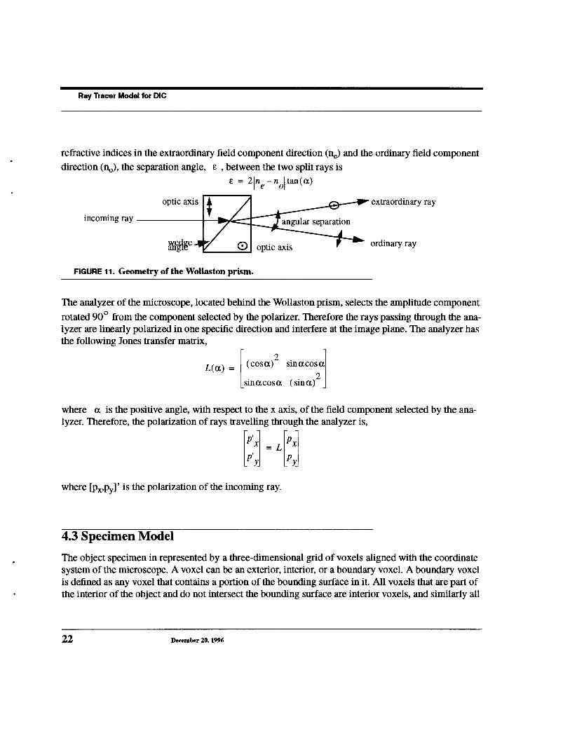
Since the transverse location of the Wollaston prism at the objective can be manipulated by the user,this prism is modeled as an object located at the back focal plane of the objective with a finite thick-hess. The prism can be shifted in the transverse plane to change the phase bias between the two inter-fering beams. The Wollaston prism1 is modeled as two wedges of quartz crystals (as shown in figure11) with a wedge angle a. The optic axes of the two wedges are orthogonal. The refraction of lightrays can be derived by applying Snell’s refraction law at the interface of the two wedges. Given the

1. Ref [33], volume 2.



refractive indices in the extraordinary field component direction (ne) and the ordinary field componentdirection (no), the separation angle, e, between the two split rays e = 2 ne-n° tan(o~)

incoming ray~ extraordinary ray

optic axis ordinary ray

FIGURE 11. Geometry of the Wollaston prism.

The analyzer of the microscope, located behind the Wollaston prism, selects the amplitude component

rotated 90° from the component selected by the polarizer. Therefore the rays passing through the ana-lyzer are linearly polarized in one specific direction and interfere at the image plane. The analyzer hasthe following Jones transfer matrix,

L((~) = (costx)2 sint~costxsint~cos(~ (sina)2

where a is the positive angle, with respect to the x axis, of the field component selected by the ana-lyzer. Therefore, the polarization of rays travelling through the analyzer is,

where [Px,Py]’ is the polarization of the incoming ray.

4.3 Specimen Model

The object specimen in represented by a three-dimensional grid of voxels aligned with the coordinatesystem of the microscope. A voxel can be an exterior, interior, or a boundary voxel. A boundary voxelis defined as any voxel that contains a portion of the bounding surface in it. All voxels that are part ofthe interior of the object and do not intersect the bounding surface are interior voxels, and similarly all


Interaction of light rays and matter

voxels that are outside the object volume are exterior voxels. The boundary voxels contain an approxi-mate surface normal, and a weighting factor (ranging from 0.0 - 1.0) that determines how much of thevoxel volume is inside the object volume. The weighting factor of the interior voxels is 1, and theweighting factor of the exterior voxels is O.

"~k.9 13 1.£ ".9~ ~

,~ 1.0 1.0

FIGURE 12. Example of a cross section of the voxel grid. The dashed lines represent the true objectshape. The vectors represent the stored normal approximations at the boundary voxels and thenumbers represent the weighting factors.

As light rays intersect the object grid, the rays scatter (either due to reflection or transmission) at theboundary voxels. The normal at the boundary voxel determines the direction of scatter. Propagation oftransmitted light rays through the interior voxels determine the phase delay of the ray by the object.

4.4 Interaction of light rays and matter

When a light ray intersects an object, it can give rise to a number of new rays according to the rough-ness on the surface of the object. The set of new rays is a result of scattering caused by surface diffrac-tion effects. The number of new rays scattered in different directions is a function of the roughnessmeasure of the surface, the angle of the incident light ray, and the wavelength of the incoming radia-tion. Any number of different surfaces can be modeled using this general paradigm. The transmissionand reflection characteristics of the surface are input into the ray tracer. This consists of the distributionof rays transmitted and reflected for incident light angles ranging from 0 to 90°, at 15 o increments ofthe incident angle. All other incident angles’ reflection and transmission characteristics are interpo-lated from the two nearest distributions stored.

For each incident angle in addition to the specified scattered rays, the specularly transmitted andreflected ray directions are computed using Snell’s propagation laws. In addition, for all specularly and


Ray Tracer Model for OIC

diffusely transmitted and reflected rays, the Fresnel reflection/transmission coefficients are used toupdate the amplitude and phase of the polarized components of the E-field.

I

I

Oi I o~

ni~ Br object

interface

FIGURE 13. Light ray propagation geometry at an object intersection point. The subscript i denotesincident, t denotes transmitted, and r denotes reflected illumination. The plane of incidence is assumedto be the plane of the paper.

As depicted in figure 13, the propagation direction of every specularly transmitted and reflected ray isobtained using Snells laws. Therefore in the plane of incidence,0i = Or and nt.sin0i = ntsinOt"

In the previous and following equations, it should be noted that the index of refraction is actuallydependent upon wavelength, but this dependence can be ignored since the ray-tracer model assumes amonochromatic wave. Written as a vector refraction equation for the transmitted ray propagationdirection kt,

ni(~i x ~n) = nt(]~t x

where un is the surface normal at the intersection point.

The Fresnel equations determine the propagation of the E-field components at the intersection of twolinear, isotropic, homogeneous media. The components of the E-field, represented by a local coordi-nate system at each ray, have to be transformed into two components perpendicular and parallel to theincident plane both of which are still perpendicular to the propagation vector. The reflected and trans-mitted fields, perpendicular and parallel to the incident plane, are weighed by the appropriate reflection


Interaction of light rays and matter

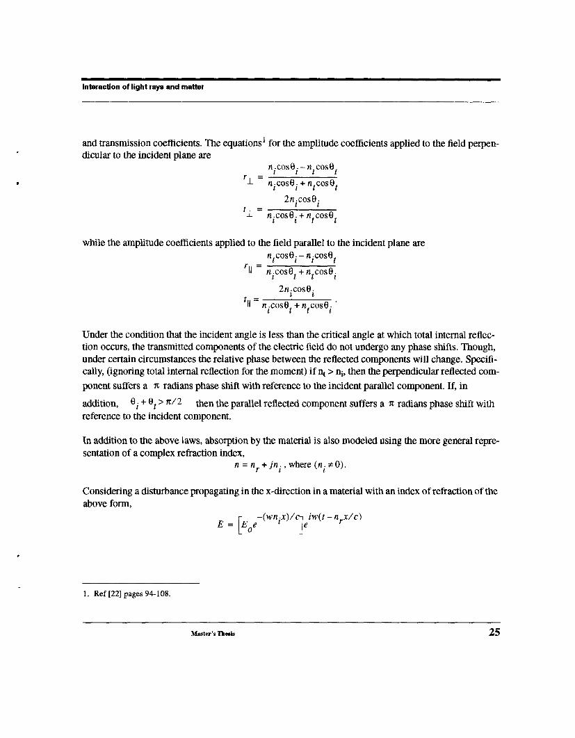
and transmission coeffcients. The equations1 for the amplitude coefficients applied to the field perpen-dicular to the incident plane are

nicosOi- ntcosOtr I = nicosOi+ ntcosOt

2n.cos0.l It± = nicosOi + ntcosOt

while the amplitude coefficients applied to the field parallel to the incident plane are

ntcosOi - nicosOtrll = nicosOt + ntcosOi

2n.cosO.tll = nicosOt + ntcosOi ¯

Under the condition that the incident angle is less than the critical angle at which total imernal reflec-tion occurs, the transmitted components of the electric field do not undergo any phase shifts. Though,under certain circumstances the relative phase between the reflected components will change. Specifi-cally, (ignoring total internal reflection for the momem) if t >ni, th en the perpendicular reflected com-ponent suffers a ~ radians phase shift with reference to the incidem parallel component. If, in

addition, 0i + 0t > r~/2 then the parallel reflected component suffers a n radians phase shift withreference to the incident component.

In addition to the above laws, absorption by the material is also modeled using the more general repre-sentation of a complex refraction index,

n = nr + jni , where (ni ~ 0).

Considering a disturbance propagating in the x-direction in a material with an index of refraction of theabove form,

r -(wnix)/~ iw(t- nrX/C)E=lEoe ~e

1. Ref [22] pages 94-108.

Master’s ~h~is 25


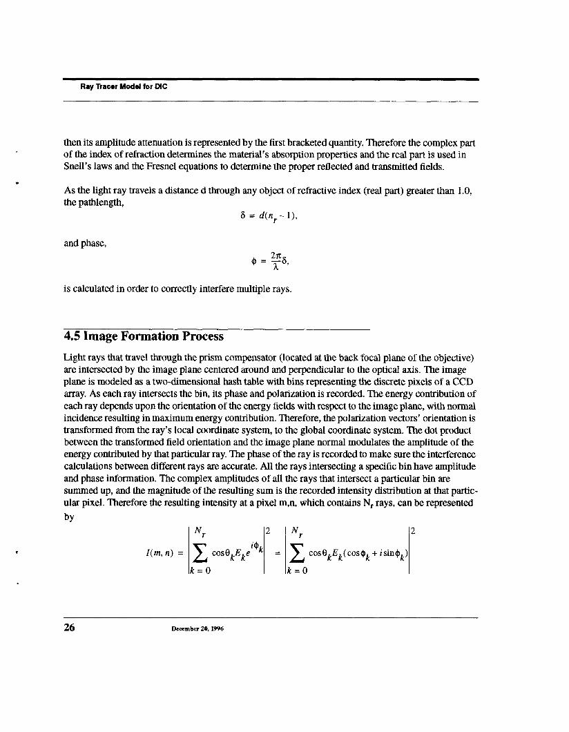
then its amplitude attenuation is represented by the first bracketed quantity. Therefore the complex partof the index of refraction determines the material’s absorption properties and the real part is used inSnell’s laws and the Fresnel equations to determine the proper reflected and transmitted fields.

As the light ray travels a distance d through any object of refractive index (real part) greater than 1.0,the pathlength,

8 = d(nr- 1),

and phase,

is calculated in order to correctly interfere multiple rays.

4.5 Image Formation Process

Light rays that travel through the prism compensator 0ocated at the back focal plane of the objective)are intersected by the image plane centered around and perpendicular to the optical axis. The imageplane is modeled as a two-dimensional hash table with bins representing the discrete pixels of a CCDarray. As each ray intersects the bin, its phase and polarization is recorded. The energy contribution ofeach ray depends upon the orientation of the energy fields with respect to the image plane, with normalincidence resulting in maximum energy contribution. Therefore, the polarization vectors’ orientation istransformed from the ray’s local coordinate system, to the global coordinate system. The dot productbetween the transformed field orientation and the image plane normal modulates the amplitude of theenergy contributed by that particular ray. The phase of the ray is recorded to make sure the interferencecalculations between different rays are accurate. All the rays intersecting a specific bin have amplitudeand phase information. The complex amplitudes of all the rays that intersect a particular bin aresummed up, and the magnitude of the resulting sum is the recorded intensity distribution at that partic-ular pixel. Therefore the resulting intensity at a pixel m,n, which contains Nr rays, can be representedby

l(m, n) = cOSOkEk(COSq~k + isin~k)k=O k=O


Im~je Formation Process

where 0k is the angle between the image plane normal and the k-th propagation vector, Ek is theamplitude and ~k is the phase of the E-field of the k-th ray.

In the presence of an infinite dimension aperture, the intensity distribution at the image plane asdescribed above would be accurate. In reality the exit pupil of the objective has a circular shape of afinite extent and therefore diffraction by the aperture has to be incorporated into the model. The abovedevelopments were modified to incorporate diffraction so that one ray contributes to more than onepixel bin. A simple Fraunhofer diffraction pattern (the Fourier integral of the exit pupil convolved withthe inverted and magnified image) cannot be used to accurately describe the image, since contributionsfrom out-of-focus object planes distort the image formed from the in focus plane. The three dimen-sional light distribution near the focus point has to be considered.

The diffraction model used, which is also discussed in detail in Born and Wolf, begins with Debye’sintegral based on the Huygens-Fresnel principle, which states that secondary spherical wavelets origi-nating at every point of a wavefront mutually interfere. The development assumes that a convergingspherical wavefront emerges through the lens aperture. This is consistent with the assumptions of geo-metrical optics claiming that the spherical wave converges at the geometrical point of focus. Thereforethe point where the refracted ray would intersect the theoretical image plane is also the point of con-vergence (zero phase) for the respective spherical wave. The theoretical image plane is defined by theGaussian lens law for thin lens,

1 1 1+ --si So fl

where si is the distance from the image plane to the lens center, so is the distance from the object planeto the lens center, and3~ is the focal length of the lens. Each ray in the ray-tracer emerging from the lensaperture is treated as a emerging spherical wavefront. To simplify the model, the phase distortions dueto the angle that each ray forms with the optic axis and its axial displacement is ignored. The point ofintersection of each ray with the image plane is convolved with a complex amplitude distribution func-tion which determines how diffraction effects convolute the spherical wavefront. Due to the asymme-tries associated with each off axis ray, the integral, in reality, is a space-variant superposition, but inthis model the integral is simplified to being a space-invafiant convolution integral. The phase devia-



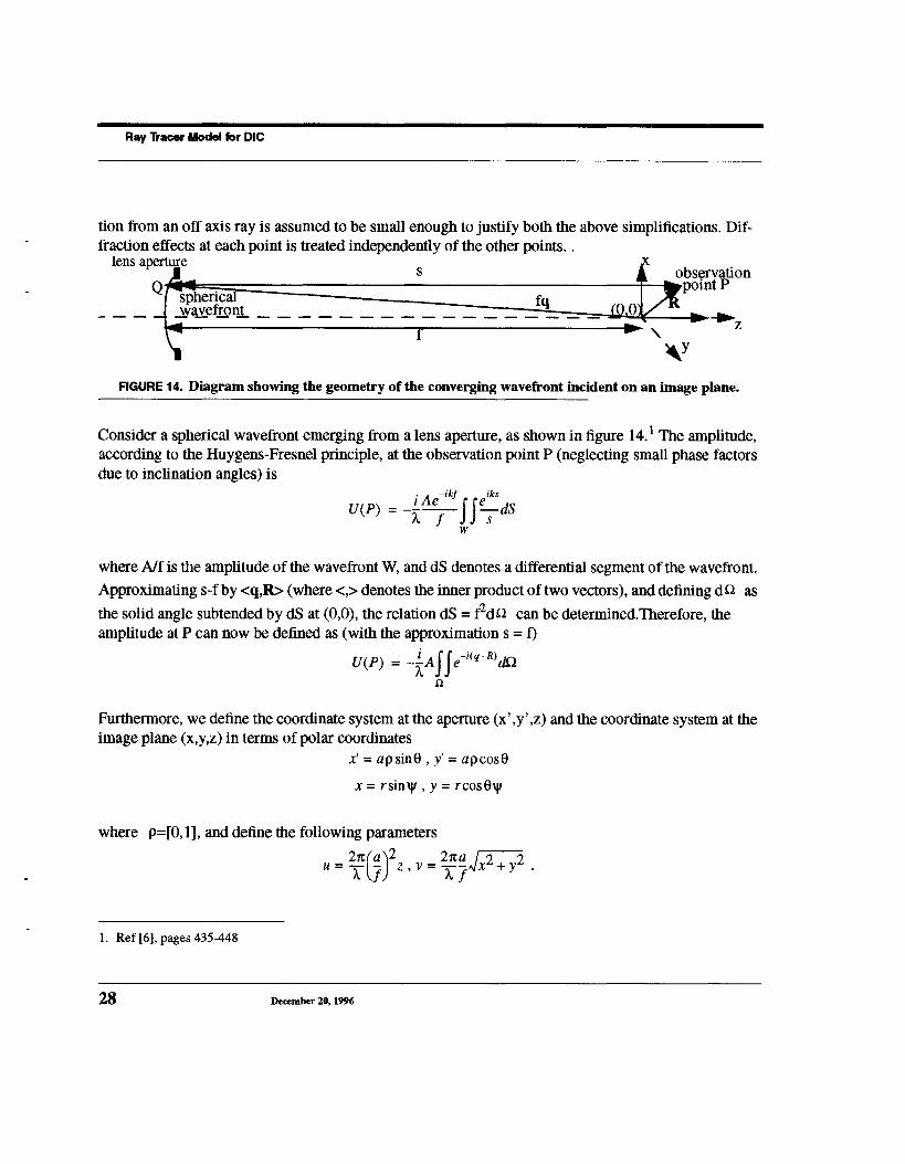
tion from an off axis ray is assumed to be small enough to justify both the above simplifications. Dif-fraction effects at each point is treated independently of the other points..

~~ observation

lens apertures

-~---~point PQfq

(0,0,L/,.._ "

q f-’-

FIGURE 14. Diagram showing the geometry of the converging wavefront incident on an image plane.

Consider a spherical wavefront emerging from a lens aperture, as shown in figure 14.1 The amplitude,according to the Huygens-Fresnel principle, at the observation point P (neglecting small phase factorsdue to inclination angles) is

i Ae-ikf ~f- -eiksU(P)=

w

where A/f is the amplitude of the wavefront W, and dS denotes a differential segment of the wavefront.Approximating s-f by <q,R> (where <,> denotes the inner product of two vectors), and defining dfl

the solid angle subtended by dS at (0,0), the relation dS = f2d~ can be determined.Therefore, theamplitude at P can now be defined as (with the approximation s = f)

U(P)= -~a~e-~(qR)d~

Furthermore, we define the coordinate system at the aperture (x’,y’,z) and the coordinate system at theimage plane (x,y,z) in terms of polar coordinates

x’ = apsin0, y’ = apcos0

x = rsin~, y = rcos0V

wh~e P=-[0,1], and define the following parameters

2n(a’~2 ~x2 + y22r~a ~2= -zt?) z, v = -z7 ¯

1. Ref [6], pages 435-448


Image Formation Process

The amplitude at P can be defined as

i Aa2e~uo ]~d~doU(P, = ~, f2 ~exp-ilvpc°s(0-~)+l

00

Here it should be noted that the integral over 0 is simply the Fraunhofer diffraction pattern on a circu-

lar aperture (equal to 2r~J0(vp) ) and that the remaining integral can be separated into real and imagi-nary parts (using Euler’s identity).

Galbraith, et. al. 1 derived the same model of the energy distribution about the focus point by followingBorn and Wolf’s development, but representing the complex integral in terms of converging series. The

diffraction calculations are based on a redefined axial parameter u= 2~t b/k, where b is the dis-

tance from the geometrical point of focus along the optical axis, and on the redefined radial parameter

v=- 2~r/k, where r is the radial distance on the image plane to the geometrical point of focus. (a/f is

the sine of half the aperture angle, or in other words, the numerical aperture of the lens divided by theindex of refraction of the lens material) The geometrical point of focus is determined by calculatingthe distance from the ray origin on the object to the lens and using this distance (so) and lens-law equa-tion to determine where the corresponding image side focal point would be. Expanding the sine, cosineand Bessel functions in terms of infinite series, the equations from section 3.1 for the complex ampli-tude K(u,v)+iL(u,v),

K(u, v) = cos(u/ f2)B(u, v) + sin(u/ f2)A(u,

L(u, v) = cos(u/ f2)A(u, v)-sin(u/ f2)B(u,

1. Ref [17]



where

A(u,v) = (_l)n_1n-

-1)! (-1) tn-1 (u/2)2tn-1(n+ 2m- 1)(2m- m=l

’~ - 1 n(_l)m-

(u/2)2m- B(u,V)

(n + 2m- 2)(2m- n=l =1

are derived in a form that can be manipulated by a computer. These equations are derived in Galbraith,et.al and will not be rederived here. Using the values of K and L as weighting factors for different u,vvalues, the complex amplitude of the ray is distributed across the neighboring pixels. For the distancecalculations, the center of the neighboring pixel to the point of intersection of the current ray is used.The weighted complex amplitude calculated at each pixel center is multiplied by the area of the pixel.

~adiallstance(r)

geometrical

poin~~

focalplane

image planeI I I

"~axial distance (b)

refracted lightray

FIGURE 15, Contribution to the shaded pixel in the image plane by the refracted light ray depends onthe axial and radial distance from the geometrical point of focus of that refracted ray.

4.6 Assumptions and Simplifications

In order to represent the wavefronts travelling through the microscope as light rays, I have assumedthat the wavefront can be accurately approximated by local planar wavefronts. The higher the sam-piing of light rays passing through the microscope optics, the smaller the size of the approximatinglocal wavefronts, and therefore the better the approximation. As long as sampling rates are sufficientlyhigh to represent the highest frequency present in the object, the sampling is justified.


Software Implementation Details

The paraxial approximation was used in the calculation of the refraction of light rays through theobjective lens and for the diffraction calculations. The diffraction calculations approximate the two-dimensional Huygens-Fresnel integral using a 2-d rectangular numerical- integration scheme in wherethe rectangles are same size as the pixels in the image plane. This approximation is justified due to thefact that the resolution in the CCD camera plane is limited by the size of the CCD pixels (which corre-sponds to the size of the pixels in the image plane of the ray tracer model). 1 In reality for the use of theFresnel integral assumes that the image is detected on a spherical surface with a radius equal to the dis-tance from the lens center to the image plane. This assumption is justified due to large distancebetween the lens center and the image plane when compared to the aperture radius of the lens and thewavelength of light. In addition, a scalar diffraction theory is applied, whereas a more rigorous vectordiffraction theory would account for the polarization of light rays. As mentioned previously, phasedeviations due to the inclination angles of the rays and the off axis location of their origins have beenignored in the current model.

4.7 Software Implementation Details

A recursive ray-tracing algorithm, accounting for the interaction of rays at multiple surfaces, was usedto build the DIC microscope model. During the first pass, a ray-tree was built from all the ray-objectinteractions. In order to create images at multiple object planes through the specimen, the ray-tree gen-erated previously was simply used to calculate the new images, therefore avoiding multiple ray-cast-ing.

The following vector-based calculation of Snell’s law is implemented. This representation requires lesscomputations at every object intersection than the analytical equation. The transmitted vector, T, andthe reflected vector, R, are functions of the surface normal vector, N, and the incident light vector, I,

sinO’lsinOic°sOil~sinOi~2~7~: -’-2t) + "sin0, ~1 + ~J(cos 0i -1)

1. Ref [71


Ray Tracer Model for DIe

where the angle subscripts i and t indicate incident and transmitted directions respectively.

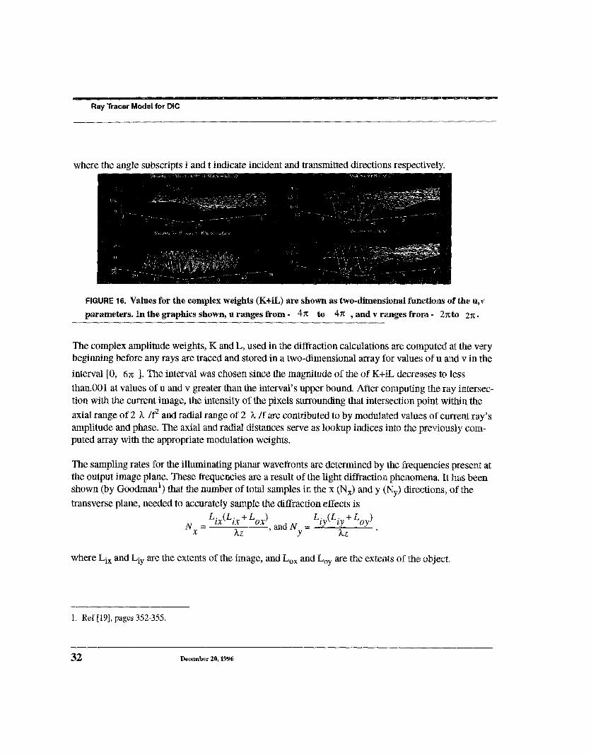
FIGURE 16. Values for the complex weights (K+iL) are shown as two-dimensional functions of theparameters. In the graphics shown, u ranges from - 4~ to 4~ , and v ranges from - 2~to 2~o

The complex amplitude weights, K and L, used in the diffraction calculations are computed at t~he verybeginning before any rays are traced and stored in a two-dimensional array for values of u and v in the

interval [0, 6r~ ]. The interval was chosen since the magnitude of the of K+JL decreases to less

than.001 at values of u and v greater than the interval’s upper bound. After computing the ray irttersec-tion with the current image, the intensity of the pixels surrounding that intersection point within theaxial range of 2 3,/re and radial range of 2 3,/f are contributed to by modulated values of current ray’samplitude and phase. The axial and radial distances serve as lookup indices ~r~to the previously com-puted array with the appropriate modulation weights.

The sampling rates for the illuminating planar wavefronts are determined by the frequencies present atthe output image plane. These frequencies are a result of the light diffraction phenomena. It has beenshown (by Goodman1) that the number of total samples in the x (Nx) and y (Ny) directions, of transverse plane, needed to accurately sample the diffraction effects is

Lix(Lix + Lox) Liy(Liy + Loy)= , and Ny = ,Nx ~,z Z,z

where Lix and Liy are the extents of the image, and Lox and Loy are the extents of the object.

1. Ref [19], pages 352-355.



A data file is used to input the general optics setup of the microscope, including the lens parameters,and prism specifications. The object type can be specified via the data file or via a Motif user interfacedialog box. The transmission and reflection properties of the object are read in via a user specified datafile. Also, certain optical configurations, including the shear direction and magnitude of the beam split-ters and the bias introduced by the translation of the compensator prism, can be changed in the ray-tracer model via another dialog box. Objects in the microscope are arranged in a spatial gr~d datastructure with uniformly sized voxel cubes. Traversal through the voxel space utilizes the traversalalgorithm developed by Amanatides and Woo. 1

FIGURE 17~ The ray-tracer’s interface showing how objects and optical configuration~ can be specified.

1. Ref [5]


SimulaUon Results

SECTION 5 Simulation Results

Originally, in order to simplify the mathematics, the ray-tracer model was implemented in two-dimen-sions, x and z, such that the z axis corresponded to the optical axis. Two-dimensional objects, such as acircle, semi-circle and a plane were simulated. In order to compare the simulated images with realdata, images of 4 micron and 10 micron diameter polystyrene beads were imaged at different objectplanes under a microscope. A cross section through the middle of the images was used to approximatethe two-dimensional plot. These plots were compared with the plots resulting from the two-dimen-sional ray-tracer.

The ray-tracer was then enhanced to simulate the microscope optics using a three-dimensional model.The 3-d version contains the full accurate descriptions of the ray-object interactions and the E-fieldpolarization. The images from the 3-d simulation are compared to the actual sphere images. The

34 December 2~, 1996


microscope used to image the beads is a Zeiss Inverted Multi-Mode microscope. I The objective lens, aZeiss Plan Neofluor, specifications are given in table 1.

FIGURE 18. Cross sections of normalized images of spheres taken using DIC optics i~ a trar~smitted fightmicroscope. The spheres have a radius of 2 microns. The sphere comes into focus from the 5th sliceabove and goes out of focus from the eight slice. This sample contained optical cement of ~:efractiveindex 1.56. In this series, the images were taken at a. 2 micron z-resolution.

1. Ref [40]

Master’sThesis 35

Simulation Results

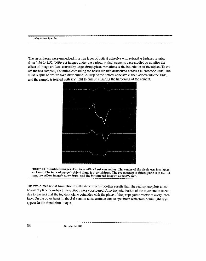
The test spheres were embedded in a thin layer of optical adhesive with refractive indexes rangingfrom 1.56 to 1.52. Different images under the various optical cements were studied to monitor theeffect of image artifacts caused by large abrupt phase variations at the boundaries of the object. To cre-ate the test samples, a solution containing the beads are first distributed across a microscope slide. Theslide is spun to ensure even distribution, A drop of the optical adhesive is then added onto the s?ide,and the sample is treated with UV light to cure it, ensuring the hardening of the cement.

FIGURE 19. Shnulated images of a circle with a 2 micron radius. The center ef the circle was located atz=.l nun. The top red image’s object plane is at z=.103mm. The green image’s object p~ane is at z=.102ram, the yellow image’s at z=.lmm, and the bottom red image’s at z=.097

The two-dimensional simulation results show much smoother results than the real sphere plots sinceno out of plane ray-object interactions were considered. Also the polarization of the rays remain linear,due to the fact that the incident plane coincides with the plane of the propagation vector at every inter-face. On the other hand, in the 3-d version noise artifacts due to specimen refraction of the light rays,appear in the simulation images.

December 20 1996

Software implementation Details

For the sphere data simulation, the impinging planar wavefronts are sampled at the z=0 plane and theobject specimen is centered at x=0, y=0, and z=. lmm. Since the maximum phase change th~:ough theobject (with reference to its containing medium) is ~/8 , the bias between the interfering wavefronts,for the corresponding simulated images shown, is set at that value. By calculating the width of theshadow-cast region in the original images when in focus, the shear separation is estimated at .75microns. Using the equations for determining sampling rates presented in section 4.7, at least 321 sam-ples in each of the x and y directions had to be taken to accurately sample the optical disturbances. Thecurrent version of the ray-tracer supports the full three-dimensionai representation of the microscopeobjects and the ray-object interactions.

FIGURE 20. The actual images of spheres (corresponding to the plots in figure 18). The sphere comesinto focus at the fifth image.

Master’s Thes~s 37

SimulaUon Results

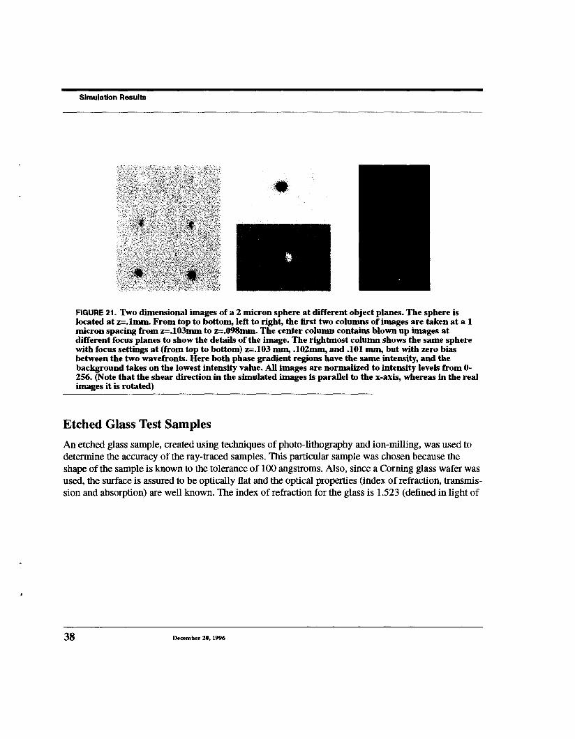
FIGURE 21. Two dimensional images of a 2 micron sphere at different object planes. The sphere islocated at z=.lmm. From top to bottom, left to right, the first two columns of images are taken at a 1micron spacing from z=.103mm to z=.098mm. The center column contains blown up images atdifferent focus planes to show the details of the image. The rightmost column shows the same spherewith focus settings at (from top to bottom) z=.103 mm, .102mm, and .101 mm, but with zero biasbetween the two wavefronts. Here both phase gradient regions have the same intensity, and thebackground takes on the lowest intensity value. All images are normalized to intensity levels from 0-256. (Note that the shear direction in the simulated images is parallel to the x-axis, whereas in the realimages it is rotated)

Etched Glass Test Samples

An etched glass sample, created using techniques of photo-lithography and ion-milling, was used todetermine the accuracy of the ray-traced samples. This particular sample was chosen because theshape of the sample is known to the tolerance of 100 angstroms. Also, since a Coming glass wafer wasused, the surface is assured to be optically fiat and the optical properties (index of refraction, transmis-sion and absorption) are well known. The index of refraction for the glass is 1.523 (defined in light



wavelength 589.3 nm) and the absorption is 7% of light intensity (for light of wavelength 640nm) lmm of glass. The circular glass wafer, diagrammed below, is .5ram thick, and 1 inch in diameter.Each square in the wafer contains several etched rectangles. Each rectangle has a depth of. 3 microns.

of entire sample a blown up square

microns

a blown up view of oneroundedrectangle

FIGURE 22. Schematic of the fabricated sample. (not to scale)

The boundaries of the rounded rectangular depression represented the areas where the phase of thetransmitted wavefront changed. Using a device that measured the depth of the etching, it was deter-mined that the boundaries of the rectangles were not perfect transition regions, but had an averageslope of 3.07. This information was included in the simulation.

True images of the fabricatedwafer as tlescribed above.

The right column of imagesis taken with an 100X oil,1.3 NA lens. The left columnis also taken with the sameobjective lens, only the images aremagnified to show details.

Each image is at a.4 micronspacing, w~here the object is infocus at the bottom most image.Note the very slow decline inimage quality as the object goesout of focus. This was consistentwith simulations of the same object.

FIGURE 23. DIC images of the etched glass wafer sample.


Simulation Results

FIGURE 24. Simulated images of etched wafer shown with at two different shear directions. The leftfigure corresponds (approximately) to the actual images shown in the previous image. The cen~erimage depicts the symmetry in the image with the shear direction normal to the object edge. Therightmost image shows the degradation in the image at an out of focus plane 10 microns above theobject.

Discussion of Results

Qualitative comparison of the real sphere data with the simulated data indicate that the in focus imageshave very similar intensity distributions, while the out of focus images do not correspond as closely.While the asymmetrical intensity distribution on planes focuses above and below the object result insimilar patterns in the simulated images, the exact effects are not reproduced. Quantitative compari-sons of images with the object in focus show that the average intensity error between normalized realand simulated images is 7.3% in the sphere data sets. With the object plane of the lens located abovethe object, the error between the real and simulated images (out-of-focus in, ages) reached 18o73%.

approximate location..... of object

FIGURE 25. The normalized left image depicts the absolute value of the error betweer~ an in-focns slicefrom the real and simulated sphere data sets. White regions indicate high error points while blackregions indicate no error. The right image depicts the error between an out-of-focus slice. The largesterrors, 28% in the first image and 42% in the second image, occurred at the periphery of the object.

40 December 20,1996


The real and simulated images of the etched glass sample had very similar intensity distributions, bothquantitatively and qualitatively. Differences between the out of focus images still resulted in highererrors than between in-focus slices.The average error between slices of images with the etching infocus was 5.4%, while the average error between out-of-focus slices was 9.35%.

FIGURE 26. The left image depicts the normalized absolute value of the error betweer~ the simulated andreal in-focus images. White depicts large errors and black depicts no errorso As can be seen, at thep|aces of significant gradient changes, the error drops significantly. The maximum error in this imagewas 18%. The normalized right image depicts the error between two o~at of focus slices, with anmaximum error of 37.19 %.

Master’s Thesis

Conclusion and Future DireclJon

SECTION 6 Conclusion and Future Direction

The ray tracer model realistically represents objects that can be imaged using a DIC transmitted-lightoptical system. By easily modeling different microscope configurations, it results in different imagesof the same object. The current system demonstrates the ability to simulate images that are close to thereal images. As can be seen from the test samples and the simulated images, the dominant features ofthe DIC image are captured by the ray tracer model. Locations on the object that exhibit significantphase changes are correctly depicted by the simulated images. In addition, the general characteristicsof out-of-focus distortions present in the simulated images, correspond to the real images.

Due to simplifications in the current microscope model, inaccuracies do occur in the simulated images.The current version of the ray tracer does not account for a condenser aperture larger than a point, andtherefore does not account for partial coherence effects. In addition, a more thorough investigation intothe space-variant phase deviation effects present due to diffraction by the lens aperture could result in amore accurate model of the light amplitude distribution at the image plane. Also, diffraction due to theobject is not represented in the current version, and could be incorporated. Since the lens in the currentray-tracer model is an ideal refracting surface, any aberration introduced by the objective is also notmodeled. By mathematically modeling the refraction of the objective lens to include different degreesof aberrations and monitoring the corresponding effects on the simulated images, it might be furtherpossible to isolate the cause of the out-of-focus asymmetries in the images.



Using the simulated images from the ray tracer model, it can be possible to estimate a volumetric rep-resentation of the specimen. By determining a meaningful error measure between the simulatedimages and the real microscope data, it is possible to iteratively update an estimated specimen model.Techniques such as the one described, have been used to reconstruct volumetric representations of anobject from different stereo images. To apply the same techniques to DIC images, the simulatedimages (using the ray lracer) can provide a forward projection from specimen estimate to image inten-sity distribution.

Master’s The~is ~

References

1. D. Agard, Y. Hiraoka and J. Sedat, Three-dimensional microscopy:image processing for high resolution sub-cellular imaging, Proceedings of SPIE, Vol. 1161, pp. 24-30, 1989.

2. R.D. Allen, G. David and G. Nomarski, The Zeiss-Nomarski differential interference equipment for transmit-ted-light microscopy, Z. wiss. Mikrosk., Vol. 69, pp 193-221., 1969.

3. R.D. Allen, N.S. Allen and J. Travis, Video-enhancedcontrast, differential interference contrast (AVEC-DIC)microscopy, CellMotility, Vol. 1, pp 291-302, 1981.

4. N. Alexopoulos, G. Francheschetti, D. Jackson, and P. Ufuntsev, ~rtual rays and applications, J. Opt. Soc.Am. A/ll:4, pp. 1513-1527. April, 1994.

5. J. Amanatides and A. Woo, A fast vogel traversal algorithm for ray tracing, Proceedings of Eurographics,pp3-11, 1987.

6. M. Born and E. Wolf, Principles of Optics, 6th ed., Pergamon Press, Oxford, 1980.

7. Y. Chen, Lens effect on synthetic image generation based on light particle theory, Visual Computer, Vol 3,125-136, 1987.

R. Chipman, Mechanics of polarization ray tracing, Optical Eng., 34:6, June 1995, pp 1636-1645.

C. Cogswell and C. Sheppa~d, Confocal differential interference contrast (DIC) microscopy, Journal ofMicroscopy, 165:1, pp 81-101, Jan. 1992.

10.R. Cook and K. Torrance, A reflectance model for computer graphics, Computer Graphics, 15:3, pp307-316,August, 1981.

11.M.L.Dias, Ray tracing interference color, IEEE Computer Graphics and Applications, March 1991, pp. 54-60.

12.N. Douglas, A. Jones, and F.van Ho~sel, Ray-based simulation of an optical interferometer, J. Opt. Soc. Am.A/12:l, pp. 124-131,Jan. 1995.

13.A. Erhardt, G. Zinser, D. Komitowski and J. Bille, Reconstructing 3-D light microscopic images by digitalimage processing, Applied Optics, 24:2, pp 194-200,Jan. 1985.

14.P. Feineigle, PhD Thesis, Carnegie Mellon University, May 1996.

15.L Foley, A. van Dam, S. Feiner and J. Hughes, Computer Graphics, 2nd ed., Addison Wesley, Massachusetts,1990.

16.W. Galbraith and G. David, An aid to understanding differential interference contrast microscopy: computersimulation, Journal of Microscopy, 108:2, pp. 147-176,Nov 1976.

17.W. Galbraith and R. Sanderson, The energy distribution about the image of a point, Microscopica Acta, 83:5,pp 395-402, Nov. 1980.

16.A. So Glassner, An Introduction to Ray Tracing, Academic Press Limited, London, 1989.

19.J.W. Goodman, Introduction to Fourier Optics, 2nd ed.,McGraw Hill Series in Electrical and Computer Engi-neering, New York, 1996.

December 20, 1996

20.W. Harris, Ray vector fieMs, prismatic effect and thick astigmatic optical systems, Optometry and Vision Sci-ence, 73:6, pp, 418-423, Feb. 1996.

21.M. Hayford and D. Brown, A building block approach to optical design software, Photonics Spectra, May1996, pp. 94-100.

22.E. Hecht, Optics, 2nd ed., Addison Wesley, Massachusetts, 1987.

23.X. He, K. Torrance, E Sillion, and D. Greenberg, A comprehensie physical model for light reflection, Com-puter Graphics, 25:4, pp. 175-186, July 1991.

24.Y. Hiraoka, J. Sedat and D. Agard, Determination of three-dimensional imaging properties of a light micro-scope system, Biophysics, J, Vol. 57, pp 325-333, Feb. 1990.

2s.T. Holmes, Maximum-likelihood image restoration adapted for noncoherent optical imaging, J. Opt. Soc.Am. A/5:5, pp. 666-673, May 1988.

26.T. Holmes and W. Levy, Signal-processing characteristics of differential-interference-contrast microscopy,Applied Optics, 26:18, pp. 3929-3938, Sep. 1987.

27.J. Keller, Geometrical theory of diffraction, J. Opt. Soc. Am., 52:2, pp. 116-130, Feb. 1961.

28.N. Kontoyannis and E Lanni, Measured and computed point spread functions for an indirect watter immer-sion objective used in three-dimensionalflourescence microscopy, Proceedings of the SPIE, Vol. 2655, 1996.

29.M. Koshy, D.A.Agard and J.W. Sedat, Solution of toeplitz systems for the restoration of 3-D optical section-ing microscopy data, Proceedings of the SPIE, Vol. 1205, pp 64-71, 1990.

30.G.A. Laub, G. Lenz, and E. Reinhardt, Three-dimensional object representation in imaging systems, OpticalEng., 24:5, pp. 901-905, Sep. 1985.

31.N. Lindlein and J. Schwider, Local wave fronts at diffractive elements, J. of Opt. Soc.of America, 10:12,pp2563-2571, Dec. 1993.

32.J. Lock, Ray scattering by an arbitrarily oriented spheriod, Applied Optics, 35:3, pp. 500-513, Jan. 1996.

33.M. Plum, Advanced Light Microscopy, Vols. 1 and 2, Elsevier Science Publishing Co., New York, 1988.

34.W.Press, S. Teukolsky, W. Vetterling and B. Flannery, Numerical Recipes in C, 2nd ed., Cambridge Univer-sity Press, Cambridge, 1992.

3s.C. Preza,D. Snyder, and J.A.Conchello, Imaging models for three-dimensional transmitted-light DIC micros-copy, Proceedings of SPIE, Vol. 2655, pp. 245-256., 1996.

36.D. Rogers and J.A. Adams, Mathematical Elements for Computer Graphics, McGraw Hill, New York, 1990.

37.W. Smith, Modern Optical Engineering, Mc Graw Hill, New York, 1990.

38.N. Streibl, Three-dimensional imaging by a microscope, J. Opt. Soc. Am. A/2:2, pp. 121-127, Feb. 1985.

39.J. Stewart, Calculus, 2nd ed., Wadsworth, Inc., California, 1991.

40.D. L. Taylor, M. Neberlof, E Lanni, and A. Waggoner, The new vision of light microscopy, American Scien-tist, Vol. 80, pp. 322-335., July 1992.

41.E. Waluschka, Polarization ray tracing, Proceedings of SPIE, Vol. 891, pp. 104-111, 1988.

December 20, 1996

42.G. Ward, Measuring and modeling anisotropic reflection, Computer Graphics, 26:2, pp. 265-272, July 1992.

43.T. Whitted, An improved illumination model for shaded display, Communication of the ACM, 23:6, pp. 343-349, June 1980.

44.L.B.Wolff and D.J.Kurlander, Ray tracing with polarization parameters, IEEE Computer Graphics andApplications, Nov. 1990, pp 44-55.

December 20, 1996

The Image Formation Process in Differential Interference ... · PDF fileThe Image Formation...

Documents

Transcript of The Image Formation Process in Differential Interference ... · PDF fileThe Image Formation...