The Ideal Risk, Uncertainty, and Performance...

AdvancedStochastic Models,

Risk Assessment,and PortfolioOptimization

The Ideal Risk, Uncertainty,and Performance Measures

SVETLOZAR T. RACHEVSTOYAN V. STOYANOV

FRANK J. FABOZZI

John Wiley & Sons, Inc.

THE FRANK J. FABOZZI SERIESFixed Income Securities, Second Edition by Frank J. FabozziFocus on Value: A Corporate and Investor Guide to Wealth Creation by James L. Grand and James

A. AbaterHandbook of Global Fixed Income Calculations by Dragomir KrginManaging a Corporate Bond Portfolio by Leland E. Crabbe and Frank J. FabozziReal Options and Option-Embedded Securities by William T. MooreCapital Budgeting: Theory and Practice by Pamela P. Peterson and Frank J. FabozziThe Exchange-Traded Funds Manual by Gary L. GastineauProfessional Perspectives on Fixed Income Portfolio Management, Volume 3 edited by Frank J. FabozziInvesting in Emerging Fixed Income Markets edited by Frank J. Fabozzi and Efstathia PilarinuHandbook of Alternative Assests by Mark J. P. AnsonThe Exchange-Trade Funds Manual by Gary L. GastineauThe Global Money Markets by Frank J. Fabozzi, Steven V. Mann, and Moorad ChoudhryThe Handbook of Financial Instruments edited by Frank J. FabozziCollateralized Debt Obligations: Structures and Analysis by Laurie S. Goodman and Frank J. FabozziInterest Rate, Term Structure, and Valuation Modeling edited by Frank J. FabozziInvestment Performance Measurement by Bruce J. FeibelThe Handbook of Equity Style Management edited by T. Daniel Coggin and Frank J. FabozziThe Theory and Practice of Investment Management edited by Frank J. Fabozzi and Harry M. MarkowitzFoundations of Economics Value Added: Second Edition by James L. GrantFinancial Management and Analysis: Second Edition by Frank J. Fabozzi and Pamela P. PetersonMeasuring and Controlling Interest Rate and Credit Risk: Second Edition by Frank J. Fabozzi, Steven

V. Mann, and Moorad ChoudhryProfessional Perspectives on Fixed Income Portfolio Management, Volume 4 edited by Frank J. FabozziThe Handbook of European Fixed Income Securities edited by Frank J. Fabozzi and Moorad ChoudhryThe Handbook of European Structured Financial Products edited by Frank J. Fabozzi and Moorad

ChoudhryThe Mathematics of Financial Modeling and Investment Management by Sergio M. Focardi and Frank

J. FabozziShort Selling: Strategies, Risk and Rewards edited by Frank J. FabozziThe Real Estate Investment Handbook by G. Timothy Haight and Daniel SingerMarket Neutral: Strategies edited by Bruce I. Jacobs and Kenneth N. LevySecurities Finance: Securities Lending and Repurchase Agreements edited by Frank J. Fabozzi and Steven

V. MannFat-Tailed and Skewed Asset Return Distributions by Svetlozar T. Rachev, Christian Menn, and Frank

J. FabozziFinancial Modeling of the Equity Market: From CAPM to Cointegration by Frank J. Fabozzi, Sergio

M. Focardi, and Petter N. KolmAdvanced Bond Portfolio management: Best Practices in Modeling and Strategies edited by Frank

J. Fabozzi, Lionel Martellini, and Philippe PriauletAnalysis of Financial Statements, Second Edition by Pamela P. Peterson and Frank J. FabozziCollateralized Debt Obligations: Structures and Analysis, Second Edition by Douglas J. Lucas, Laurie

S. Goodman, and Frank J. FabozziHandbook of Alternative Assets, Second Edition by Mark J. P. AnsonIntroduction to Structured Finance by Frank J. Fabozzi, Henry A. Davis, and Moorad ChoudhryFinancial Econometrics by Svetlozar T. Rachev, Stefan Mittnik, Frank J. Fabozzi, Sergio M. Focardi, and

Teo JasicDevelopments in Collateralized Debt Obligations: New Products and Insights by Douglas J. Lucas, Laurie

S. Goodman, Frank J. Fabozzi, and Rebecca J. ManningRobust Portfolio Optimization and Management by Frank J. Fabozzi, Peter N. Kolm, Dessislava

A. Pachamanova, and Sergio M. FocardiAdvanced Stochastic Models, Risk Assessment, and Portfolio Optimization by Svetlozar T. Rachev, Stoyan

V. Stoyanov, and Frank J. FabozziHow to Select Investment Managers and Evalute Performance by G. Timothy Haight, Stephen O. Morrell,

and Glenn E. RossBayesian Methods in Finance by Svetlozar T. Rachev, John S. J. Hsu, Biliana S. Bagasheva, and Frank

J. Fabozzi



The Ideal Risk, Uncertainty,and Performance Measures

SVETLOZAR T. RACHEVSTOYAN V. STOYANOV

FRANK J. FABOZZI

John Wiley & Sons, Inc.

Copyright c© 2008 by John Wiley & Sons, Inc. All rights reserved.

Published by John Wiley & Sons, Inc., Hoboken, New Jersey.Published simultaneously in Canada.

No part of this publication may be reproduced, stored in a retrieval system, or transmitted inany form or by any means, electronic, mechanical, photocopying, recording, scanning, orotherwise, except as permitted under Section 107 or 108 of the 1976 United States CopyrightAct, without either the prior written permission of the Publisher, or authorization throughpayment of the appropriate per-copy fee to the Copyright Clearance Center, Inc., 222Rosewood Drive, Danvers, MA 01923, (978) 750-8400, fax (978) 750-4470, or on the Webat www.copyright.com. Requests to the Publisher for permission should be addressed to thePermissions Department, John Wiley & Sons, Inc., 111 River Street, Hoboken, NJ 07030,(201) 748-6011, fax (201) 748-6008, or online at http://www.wiley.com/go/permission.

Limit of Liability/Disclaimer of Warranty: While the publisher and author have used theirbest efforts in preparing this book, they make no representations or warranties with respect tothe accuracy or completeness of the contents of this book and specifically disclaim any impliedwarranties of merchantability or fitness for a particular purpose. No warranty may be createdor extended by sales representatives or written sales materials. The advice and strategiescontained herein may not be suitable for your situation. You should consult with aprofessional where appropriate. Neither the publisher nor author shall be liable for any loss ofprofit or any other commercial damages, including but not limited to special, incidental,consequential, or other damages.

For general information on our other products and services or for technical support, pleasecontact our Customer Care Department within the United States at (800) 762-2974, outsidethe United States at (317) 572-3993, or fax (317) 572-4002.

Wiley also publishes its books in a variety of electronic formats. Some content that appears inprint may not be available in electronic books. For more information about Wiley products,visit our Web site at www.wiley.com.

ISBN: 978-0-470-05316-4

Printed in the United States of America.

10 9 8 7 6 5 4 3 2 1

www.wiley.com

STRTo my children, Boryana and Vladimir

SVSTo my parents, Veselin and Evgeniya Kolevi, and my

brother, Pavel Stoyanov

FJFTo the memory of my parents,Josephine and Alfonso Fabozzi

Contents

Preface xiii

Acknowledgments xv

About the Authors xvii

CHAPTER 1Concepts of Probability 1

1.1 Introduction 11.2 Basic Concepts 21.3 Discrete Probability Distributions 2

1.3.1 Bernoulli Distribution 31.3.2 Binomial Distribution 31.3.3 Poisson Distribution 4

1.4 Continuous Probability Distributions 51.4.1 Probability Distribution Function, Probability

Density Function, and Cumulative DistributionFunction 5

1.4.2 The Normal Distribution 81.4.3 Exponential Distribution 101.4.4 Student’s t-distribution 111.4.5 Extreme Value Distribution 121.4.6 Generalized Extreme Value Distribution 12

1.5 Statistical Moments and Quantiles 131.5.1 Location 131.5.2 Dispersion 131.5.3 Asymmetry 131.5.4 Concentration in Tails 141.5.5 Statistical Moments 141.5.6 Quantiles 161.5.7 Sample Moments 16

1.6 Joint Probability Distributions 171.6.1 Conditional Probability 181.6.2 Definition of Joint Probability Distributions 19

vii

viii CONTENTS

1.6.3 Marginal Distributions 191.6.4 Dependence of Random Variables 201.6.5 Covariance and Correlation 201.6.6 Multivariate Normal Distribution 211.6.7 Elliptical Distributions 231.6.8 Copula Functions 25

1.7 Probabilistic Inequalities 301.7.1 Chebyshev’s Inequality 301.7.2 Frechet-Hoeffding Inequality 31

1.8 Summary 32

CHAPTER 2Optimization 35

2.1 Introduction 352.2 Unconstrained Optimization 36

2.2.1 Minima and Maxima of a DifferentiableFunction 37

2.2.2 Convex Functions 402.2.3 Quasiconvex Functions 46

2.3 Constrained Optimization 482.3.1 Lagrange Multipliers 492.3.2 Convex Programming 522.3.3 Linear Programming 552.3.4 Quadratic Programming 57

2.4 Summary 58

CHAPTER 3Probability Metrics 61

3.1 Introduction 613.2 Measuring Distances: The Discrete Case 62

3.2.1 Sets of Characteristics 633.2.2 Distribution Functions 643.2.3 Joint Distribution 68

3.3 Primary, Simple, and Compound Metrics 723.3.1 Axiomatic Construction 733.3.2 Primary Metrics 743.3.3 Simple Metrics 753.3.4 Compound Metrics 843.3.5 Minimal and Maximal Metrics 86

3.4 Summary 903.5 Technical Appendix 90

Contents ix

3.5.1 Remarks on the Axiomatic Construction ofProbability Metrics 91

3.5.2 Examples of Probability Distances 943.5.3 Minimal and Maximal Distances 99

CHAPTER 4Ideal Probability Metrics 103

4.1 Introduction 1034.2 The Classical Central Limit Theorem 105

4.2.1 The Binomial Approximation to the NormalDistribution 105

4.2.2 The General Case 1124.2.3 Estimating the Distance from the Limit

Distribution 1184.3 The Generalized Central Limit Theorem 120

4.3.1 Stable Distributions 1204.3.2 Modeling Financial Assets with Stable

Distributions 1224.4 Construction of Ideal Probability Metrics 124

4.4.1 Definition 1254.4.2 Examples 126


4.6.1 The CLT Conditions 1314.6.2 Remarks on Ideal Metrics 133

CHAPTER 5Choice under Uncertainty 139

5.1 Introduction 1395.2 Expected Utility Theory 141

5.2.1 St. Petersburg Paradox 1415.2.2 The von Neumann–Morgenstern Expected

Utility Theory 1435.2.3 Types of Utility Functions 145

5.3 Stochastic Dominance 1475.3.1 First-Order Stochastic Dominance 1485.3.2 Second-Order Stochastic Dominance 1495.3.3 Rothschild-Stiglitz Stochastic Dominance 1505.3.4 Third-Order Stochastic Dominance 1525.3.5 Efficient Sets and the Portfolio Choice Problem 1545.3.6 Return versus Payoff 154

x CONTENTS

5.4 Probability Metrics and Stochastic Dominance 1575.5 Summary 1615.6 Technical Appendix 161

5.6.1 The Axioms of Choice 1615.6.2 Stochastic Dominance Relations of Order n 1635.6.3 Return versus Payoff and Stochastic Dominance 1645.6.4 Other Stochastic Dominance Relations 166

CHAPTER 6Risk and Uncertainty 171

6.1 Introduction 1716.2 Measures of Dispersion 174

6.2.1 Standard Deviation 1746.2.2 Mean Absolute Deviation 1766.2.3 Semistandard Deviation 1776.2.4 Axiomatic Description 1786.2.5 Deviation Measures 179

6.3 Probability Metrics and Dispersion Measures 1806.4 Measures of Risk 181

6.4.1 Value-at-Risk 1826.4.2 Computing Portfolio VaR in Practice 1866.4.3 Backtesting of VaR 1926.4.4 Coherent Risk Measures 194

6.5 Risk Measures and Dispersion Measures 1986.6 Risk Measures and Stochastic Orders 1996.7 Summary 2006.8 Technical Appendix 201

6.8.1 Convex Risk Measures 2016.8.2 Probability Metrics and Deviation Measures 202

CHAPTER 7Average Value-at-Risk 207

7.1 Introduction 2077.2 Average Value-at-Risk 2087.3 AVaR Estimation from a Sample 2147.4 Computing Portfolio AVaR in Practice 216

7.4.1 The Multivariate Normal Assumption 2167.4.2 The Historical Method 2177.4.3 The Hybrid Method 2177.4.4 The Monte Carlo Method 218

7.5 Backtesting of AVaR 220

Contents xi

7.6 Spectral Risk Measures 2227.7 Risk Measures and Probability Metrics 2247.8 Summary 2277.9 Technical Appendix 227

7.9.1 Characteristics of Conditional LossDistributions 228

7.9.2 Higher-Order AVaR 2307.9.3 The Minimization Formula for AVaR 2327.9.4 AVaR for Stable Distributions 2357.9.5 ETL versus AVaR 2367.9.6 Remarks on Spectral Risk Measures 241

CHAPTER 8Optimal Portfolios 245

8.1 Introduction 2458.2 Mean-Variance Analysis 247

8.2.1 Mean-Variance Optimization Problems 2478.2.2 The Mean-Variance Efficient Frontier 2518.2.3 Mean-Variance Analysis and SSD 2548.2.4 Adding a Risk-Free Asset 256

8.3 Mean-Risk Analysis 2588.3.1 Mean-Risk Optimization Problems 2598.3.2 The Mean-Risk Efficient Frontier 2628.3.3 Mean-Risk Analysis and SSD 2668.3.4 Risk versus Dispersion Measures 267


8.5.1 Types of Constraints 2748.5.2 Quadratic Approximations to Utility Functions 2768.5.3 Solving Mean-Variance Problems in Practice 2788.5.4 Solving Mean-Risk Problems in Practice 2798.5.5 Reward-Risk Analysis 281

CHAPTER 9Benchmark Tracking Problems 287

9.1 Introduction 2879.2 The Tracking Error Problem 2889.3 Relation to Probability Metrics 2929.4 Examples of r.d. Metrics 2969.5 Numerical Example 3009.6 Summary 304

xii CONTENTS

9.7 Technical Appendix 3049.7.1 Deviation Measures and r.d. Metrics 3059.7.2 Remarks on the Axioms 3059.7.3 Minimal r.d. Metrics 3079.7.4 Limit Cases of L∗

p(X, Y) and �∗p(X, Y) 310

9.7.5 Computing r.d. Metrics in Practice 311

CHAPTER 10Performance Measures 317

10.1 Introduction 31710.2 Reward-to-Risk Ratios 318

10.2.1 RR Ratios and the Efficient Portfolios 32010.2.2 Limitations in the Application of

Reward-to-Risk Ratios 32410.2.3 The STARR 32510.2.4 The Sortino Ratio 32910.2.5 The Sortino-Satchell Ratio 33010.2.6 A One-Sided Variability Ratio 33110.2.7 The Rachev Ratio 332

10.3 Reward-to-Variability Ratios 33310.3.1 RV Ratios and the Efficient Portfolios 33510.3.2 The Sharpe Ratio 33710.3.3 The Capital Market Line and the Sharpe Ratio 340


10.5.1 Extensions of STARR 34310.5.2 Quasiconcave Performance Measures 34510.5.3 The Capital Market Line and Quasiconcave

Ratios 35310.5.4 Nonquasiconcave Performance Measures 35610.5.5 Probability Metrics and Performance Measures 357

Index 361

Preface

M odern portfolio theory, as pioneered in the 1950s by Harry Markowitz,is well adopted by the financial community. In spite of the fundamental

shortcomings of mean-variance analysis, it remains a basic tool in theindustry.

Since the 1990s, significant progress has been made in developing theconcept of a risk measure from both a theoretical and a practical viewpoint.This notion has evolved into a materially different form from the originalidea behind mean-variance analysis. As a consequence, the distinctionbetween risk and uncertainty, which translates into a distinction between arisk measure and a dispersion measure, offers a new way of looking at theproblem of optimal portfolio selection.

As concepts develop, other tools become appropriate to exploringevolved ideas than existing techniques. In applied finance, these tools arebeing imported from mathematics. That said, we believe that probabil-ity metrics, which is a field in probability theory, will turn out to bewell-positioned for the study and further development of the quantitativeaspects of risk and uncertainty. Going one step further, we make a parallel.In the theory of probability metrics, there exists a concept known as an idealprobability metric. This is a quantity best suited for the study of a givenapproximation problem in probability or stochastic processes. We believethat the ideas behind this concept can be borrowed and applied in the fieldof asset management to construct an ideal risk measure that would be idealfor a given optimal portfolio selection problem.

The development of probability metrics as a branch of probabilitytheory started in the 1950s, even though its basic ideas were used during thefirst half of the 20th century. Its application to problems is connected withthis fundamental question: ‘‘Is the proposed stochastic model a satisfactoryapproximation to the real model and, if so, within what limits?’’ In finance,we assume a stochastic model for asset return distributions and, in order toestimate portfolio risk, we sample from the fitted distribution. Then we usethe generated simulations to evaluate the portfolio positions and, finally, tocalculate portfolio risk. In this context, there are two issues arising on twodifferent levels. First, the assumed stochastic model should be close to theempirical data. That is, we need a realistic model in the first place. Second,the generated scenarios should be sufficiently many in order to represent a

xiii

xiv PREFACE

good approximation model to the assumed stochastic model. In this way,we are sure that the computed portfolio risk numbers are close to what theywould be had the problem been analytically tractable.

This book provides a gentle introduction into the theory of probabilitymetrics and the problem of optimal portfolio selection, which is consideredin the general context of risk and reward measures. We illustrate in numerousexamples the basic concepts and where more technical knowledge is needed,an appendix is provided.

The book is organized in the following way. Chapters 1 and 2 con-tain introductory material from the fields of probability and optimizationtheory. Chapter 1 is necessary for understanding the general ideas behindprobability metrics covered in Chapter 3 and ideal probability metrics inparticular described in Chapter 4. The material in Chapter 2 is used whendiscussing optimal portfolio selection problems in Chapters 8, 9, and 10.We demonstrate how probability metrics can be applied to certain areas infinance in the following chapters:

■ Chapter 5—stochastic dominance orders.■ Chapter 6—the construction of risk and dispersion measures.■ Chapter 7—problems involving average value-at-risk and spectral risk

measures in particular.■ Chapter 8—reward-risk analysis generalizing mean-variance analysis.■ Chapter 9—the problem of benchmark tracking.■ Chapter 10—the construction of performance measures.

Chapters 5, 6, and 7 are also a prerequisite for the material in the lastthree chapters. Chapter 5 describes expected utility theory and stochasticdominance orders. The focus in Chapter 6 is on general dispersion measuresand risk measures. Finally, in Chapter 7 we discuss the average value-at-riskand spectral risk measures, which are two particular families of coherentrisk measures considered in Chapter 6.

The classical mean-variance analysis and the more general mean-riskanalysis are explored in Chapter 8. We consider the structure of the efficientportfolios when average value-at-risk is selected as a risk measure. Chapter9 is focused on the benchmark tracking problem. We generalize significantlythe problem applying the methods of probability metrics. In Chapter 10,we discuss performance measures in the general framework of reward-riskanalysis. We consider classes of performance measures that lead to practicaloptimal portfolio problems.

Svetlozar T. RachevStoyan V. Stoyanov

Frank J. Fabozzi

Acknowledgments

S vetlozar Rachev’s research was supported by grants from the Divi-sion of Mathematical, Life and Physical Sciences, College of Letters

and Science, University of California–Santa Barbara, and the DeutschenForschungsgemeinschaft.

Stoyan Stoyanov thanks the R&D team at FinAnalytica for the encour-agement and the chair of Statistics, Econometrics and Mathematical Financeat the University of Karlsruhe for the hospitality extended to him.

Lastly, Frank Fabozzi thanks Yale’s International Center for Financefor its support in completing this book.

Svetlozar T. RachevStoyan V. Stoyanov

Frank J. Fabozzi

xv

About the Authors

S vetlozar (Zari) T. Rachev completed his Ph.D. in 1979 from MoscowState (Lomonosov) University, and his doctor of science degree in

1986 from Steklov Mathematical Institute in Moscow. Currently, he isChair-Professor in Statistics, Econometrics and Mathematical Finance atthe University of Karlsruhe in the School of Economics and Business Engi-neering. He is also Professor Emeritus at the University of California–SantaBarbara in the Department of Statistics and Applied Probability. He haspublished seven monographs, eight handbooks and special-edited volumes,and over 250 research articles. His recently coauthored books publishedby John Wiley & Sons in mathematical finance and financial econometricsinclude Fat-Tailed and Skewed Asset Return Distributions: Implicationsfor Risk Management, Portfolio Selection, and Option Pricing (2005);Operational Risk: A Guide to Basel II Capital Requirements, Models, andAnalysis (2007); Financial Econometrics: From Basics to Advanced Model-ing Techniques (2007); and Bayesian Methods in Finance (2008). ProfessorRachev is cofounder of Bravo Risk Management Group specializing infinancial risk-management software. Bravo Group was recently acquired byFinAnalytica, for which he currently serves as chief scientist.

Stoyan V. Stoyanov is the chief financial researcher at FinAnalytica special-izing in financial risk management software. He completed his Ph.D. withhonors in 2005 from the School of Economics and Business Engineering(Chair of Statistics, Econometrics and Mathematical Finance) at the Uni-versity of Karlsruhe and is author and coauthor of numerous papers. Hisresearch interests include probability theory, heavy-tailed modeling in thefield of finance, and optimal portfolio theory. His articles have appearedin the Journal of Banking and Finance, Applied Mathematical Finance,Applied Financial Economics, and International Journal of Theoretical andApplied Finance. Dr. Stoyanov has years of experience in applying optimalportfolio theory and market risk estimation methods when solving practicalclient problems at FinAnalytica.

Frank J. Fabozzi is professor in the practice of finance in the School ofManagement at Yale University. Prior to joining the Yale faculty, he was avisiting professor of finance in the Sloan School at MIT. Professor Fabozzi

xvii

xviii ABOUT THE AUTHORS

is a Fellow of the International Center for Finance at Yale University andis on the Advisory Council for the Department of Operations Researchand Financial Engineering at Princeton University. He is the editor of theJournal of Portfolio Management. His recently coauthored books publishedby John Wiley & Sons in mathematical finance and financial econometricsinclude The Mathematics of Financial Modeling and Investment Manage-ment (2004); Financial Modeling of the Equity Market: From CAPM toCointegration (2006); Robust Portfolio Optimization and Management(2007); Financial Econometrics: From Basics to Advanced Modeling Tech-niques (2007); and Bayesian Methods in Finance (2008). He earned adoctorate in economics from the City University of New York in 1972.In 2002, Professor Fabozzi was inducted into the Fixed Income AnalystsSociety’s Hall of Fame and is the 2007 recipient of the C. Stewart SheppardAward given by the CFA Institute. He earned the designation of CharteredFinancial Analyst and Certified Public Accountant.

CHAPTER 1Concepts of Probability

1.1 INTRODUCTION

Will Microsoft’s stock return over the next year exceed 10%? Will theone-month London Interbank Offered Rate (LIBOR) three months fromnow exceed 4%? Will Ford Motor Company default on its debt obligationssometime over the next five years? Microsoft’s stock return over the nextyear, one-month LIBOR three months from now, and the default of FordMotor Company on its debt obligations are each variables that exhibitrandomness. Hence these variables are referred to as random variables.1 Inthis chapter, we see how probability distributions are used to describe thepotential outcomes of a random variable, the general properties of prob-ability distributions, and the different types of probability distributions.2

Random variables can be classified as either discrete or continuous. Webegin with discrete probability distributions and then proceed to continuousprobability distributions.

1The precise mathematical definition is that a random variable is a measurablefunction from a probability space into the set of real numbers. In this chapter, thereader will repeatedly be confronted with imprecise definitions. The authors haveintentionally chosen this way for a better general understandability and for the sakeof an intuitive and illustrative description of the main concepts of probability theory.In order to inform about every occurrence of looseness and lack of mathematicalrigor, we have furnished most imprecise definitions with a footnote giving a referenceto the exact definition.2For more detailed and/or complementary information, the reader is referredto the textbooks of Larsen and Marx (1986), Shiryaev (1996), and Billingsley(1995).

1

2 ADVANCED STOCHASTIC MODELS

1.2 BASIC CONCEPTS

An outcome for a random variable is the mutually exclusive potential resultthat can occur. The accepted notation for an outcome is the Greek letter ω.A sample space is a set of all possible outcomes. The sample space isdenoted by �. The fact that a given outcome ωi belongs to the sample spaceis expressed by ωi ∈ �. An event is a subset of the sample space and can berepresented as a collection of some of the outcomes.3 For example, considerMicrosoft’s stock return over the next year. The sample space containsoutcomes ranging from 100% (all the funds invested in Microsoft’s stockwill be lost) to an extremely high positive return. The sample space canbe partitioned into two subsets: outcomes where the return is less than orequal to 10% and a subset where the return exceeds 10%. Consequently,a return greater than 10% is an event since it is a subset of the samplespace. Similarly, a one-month LIBOR three months from now that exceeds4% is an event. The collection of all events is usually denoted by A. In thetheory of probability, we consider the sample space � together with the setof events A, usually written as (�, A), because the notion of probability isassociated with an event.4

1.3 DISCRETE PROBABILITY DISTRIBUTIONS

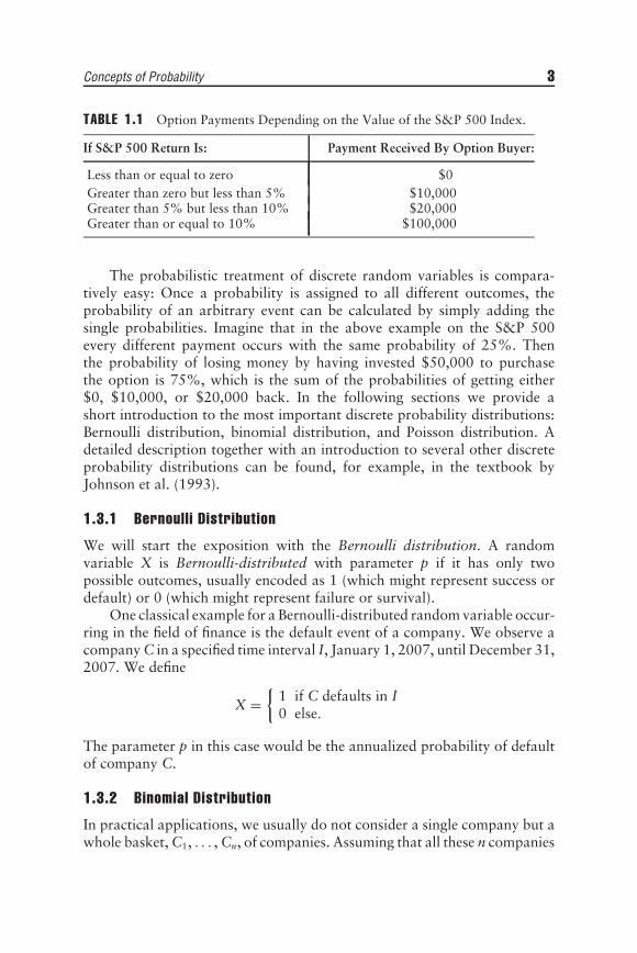
As the name indicates, a discrete random variable limits the outcomes wherethe variable can only take on discrete values. For example, consider thedefault of a corporation on its debt obligations over the next five years. Thisrandom variable has only two possible outcomes: default or nondefault.Hence, it is a discrete random variable. Consider an option contract wherefor an upfront payment (i.e., the option price) of $50,000, the buyer of thecontract receives the payment given in Table 1.1 from the seller of the optiondepending on the return on the S&P 500 index. In this case, the randomvariable is a discrete random variable but on the limited number of outcomes.

3Precisely, only certain subsets of the sample space are called events. In the casethat the sample space is represented by a subinterval of the real numbers, the eventsconsist of the so-called ‘‘Borel sets.’’ For all practical applications, we can think ofBorel sets as containing all subsets of the sample space. In this case, the sample spacetogether with the set of events is denoted by (R, B). Shiryaev (1996) provides aprecise definition.4Probability is viewed as a function endowed with certain properties, taking eventsas an argument and providing their probabilities as a result. Thus, according to themathematical construction, probability is defined on the elements of the set A (calledsigma-field or sigma-algebra) taking values in the interval [0, 1], P : A → [0, 1].

Concepts of Probability 3

TABLE 1.1 Option Payments Depending on the Value of the S&P 500 Index.

If S&P 500 Return Is: Payment Received By Option Buyer:

Less than or equal to zero $0Greater than zero but less than 5% $10,000Greater than 5% but less than 10% $20,000Greater than or equal to 10% $100,000

The probabilistic treatment of discrete random variables is compara-tively easy: Once a probability is assigned to all different outcomes, theprobability of an arbitrary event can be calculated by simply adding thesingle probabilities. Imagine that in the above example on the S&P 500every different payment occurs with the same probability of 25%. Thenthe probability of losing money by having invested $50,000 to purchasethe option is 75%, which is the sum of the probabilities of getting either$0, $10,000, or $20,000 back. In the following sections we provide ashort introduction to the most important discrete probability distributions:Bernoulli distribution, binomial distribution, and Poisson distribution. Adetailed description together with an introduction to several other discreteprobability distributions can be found, for example, in the textbook byJohnson et al. (1993).

1.3.1 Bernoulli Distribution

We will start the exposition with the Bernoulli distribution. A randomvariable X is Bernoulli-distributed with parameter p if it has only twopossible outcomes, usually encoded as 1 (which might represent success ordefault) or 0 (which might represent failure or survival).

One classical example for a Bernoulli-distributed random variable occur-ring in the field of finance is the default event of a company. We observe acompany C in a specified time interval I, January 1, 2007, until December 31,2007. We define

X ={

1 if C defaults in I0 else.

The parameter p in this case would be the annualized probability of defaultof company C.

1.3.2 Binomial Distribution

In practical applications, we usually do not consider a single company but awhole basket, C1, . . . , Cn, of companies. Assuming that all these n companies


have the same annualized probability of default p, this leads to a naturalgeneralization of the Bernoulli distribution called binomial distribution. Abinomial distributed random variable Y with parameters n and p is obtainedas the sum of n independent5 and identically Bernoulli-distributed randomvariables X1, . . . , Xn. In our example, Y represents the total number ofdefaults occurring in the year 2007 observed for companies C1, . . . , Cn.Given the two parameters, the probability of observing k, 0 ≤ k ≤ n defaultscan be explicitly calculated as follows:

P(Y = k) =(

nk

)pk(1 − p)n − k,

where(

nk

)= n!

(n − k)!k!.

Recall that the factorial of a positive integer n is denoted by n! and is equalto n(n − 1)(n − 2) · . . . · 2 · 1.

Bernoulli distribution and binomial distribution are revisited inChapter 4 in connection with a fundamental result in the theory of proba-bility called the Central Limit Theorem. Shiryaev (1996) provides a formaldiscussion of this important result.

1.3.3 Poisson Distribution

The last discrete distribution that we consider is the Poisson distribution.The Poisson distribution depends on only one parameter, λ, and can beinterpreted as an approximation to the binomial distribution when theparameter p is a small number.6 A Poisson-distributed random variable isusually used to describe the random number of events occurring over acertain time interval. We used this previously in terms of the number ofdefaults. One main difference compared to the binomial distribution is thatthe number of events that might occur is unbounded, at least theoretically.The parameter λ indicates the rate of occurrence of the random events, thatis, it tells us how many events occur on average per unit of time.

5A definition of what independence means is provided in Section 1.6.4. The readermight think of independence as no interference between the random variables.6The approximation of Poisson to the binomial distribution concerns the so-calledrare events. An event is called rare if the probability of its occurrence is close to zero.The probability of a rare event occurring in a sequence of independent trials can beapproximately calculated with the formula of the Poisson distribution.


The probability distribution of a Poisson-distributed random variableN is described by the following equation:

P(N = k) = λk

k!e−λ, k = 0, 1, 2, . . .

1.4 CONTINUOUS PROBABILITY DISTRIBUTIONS

If the random variable can take on any possible value within the rangeof outcomes, then the probability distribution is said to be a continuousrandom variable.7 When a random variable is either the price of or the returnon a financial asset or an interest rate, the random variable is assumed tobe continuous. This means that it is possible to obtain, for example, a priceof 95.43231 or 109.34872 and any value in between. In practice, we knowthat financial assets are not quoted in such a way. Nevertheless, there isno loss in describing the random variable as continuous and in many timestreating the return as a continuous random variable means substantial gainin mathematical tractability and convenience. For a continuous randomvariable, the calculation of probabilities is substantially different from thediscrete case. The reason is that if we want to derive the probability thatthe realization of the random variable lays within some range (i.e., overa subset or subinterval of the sample space), then we cannot proceed in asimilar way as in the discrete case: The number of values in an interval is solarge, that we cannot just add the probabilities of the single outcomes. Thenew concept needed is explained in the next section.

1.4.1 Probability Distribution Function, ProbabilityDensity Function, and Cumulative Distribution Function

A probability distribution function P assigns a probability P(A) for everyevent A, that is, of realizing a value for the random value in any specifiedsubset A of the sample space. For example, a probability distributionfunction can assign a probability of realizing a monthly return that isnegative or the probability of realizing a monthly return that is greater than0.5% or the probability of realizing a monthly return that is between 0.4%and 1.0%.

7Precisely, not every random variable taking its values in a subinterval of the realnumbers is continuous. The exact definition requires the existence of a densityfunction such as the one that we use later in this chapter to calculate probabilities.


To compute the probability, a mathematical function is needed torepresent the probability distribution function. There are several possibilitiesof representing a probability distribution by means of a mathematicalfunction. In the case of a continuous probability distribution, the mostpopular way is to provide the so-called probability density function orsimply density function.

In general, we denote the density function for the random variable Xas f X(x). Note that the letter x is used for the function argument and theindex denotes that the density function corresponds to the random variableX. The letter x is the convention adopted to denote a particular value forthe random variable. The density function of a probability distribution isalways nonnegative and as its name indicates: Large values for f X(x) ofthe density function at some point x imply a relatively high probability ofrealizing a value in the neighborhood of x, whereas f X(x) = 0 for all x insome interval (a, b) implies that the probability for observing a realizationin (a, b) is zero.

Figure 1.1 aids in understanding a continuous probability distribution.The shaded area is the probability of realizing a return less than b andgreater than a. As probabilities are represented by areas under the densityfunction, it follows that the probability for every single outcome of acontinuous random variable always equals zero. While the shaded area

0

0.05

0.1

0.15

0.2

0.25

0.3

0.35

0.4

x

f X(x

)

a b

FIGURE 1.1 The probability of the event that a givenrandom variable, X, is between two real numbers, a andb, which is equal to the shaded area under the densityfunction, f X(x).


in Figure 1.1 represents the probability associated with realizing a returnwithin the specified range, how does one compute the probability? This iswhere the tools of calculus are applied. Calculus involves differentiationand integration of a mathematical function. The latter tool is called integralcalculus and involves computing the area under a curve. Thus the probabilitythat a realization from a random variable is between two real numbers aand b is calculated according to the formula,

P(a ≤ X ≤ b) =∫ b

afX(x)dx.

The mathematical function that provides the cumulative probability ofa probability distribution, that is, the function that assigns to every realvalue x the probability of getting an outcome less than or equal to x, is calledthe cumulative distribution function or cumulative probability function orsimply distribution function and is denoted mathematically by FX(x). Acumulative distribution function is always nonnegative, nondecreasing, andas it represents probabilities it takes only values between zero and one.8 Anexample of a distribution function is given in Figure 1.2.

0

1

x

FX

(x)

a b

FX(a)

FX(b)

FIGURE 1.2 The probability of the event that agiven random variable X is between two realnumbers a and b is equal to the differenceFX(b) − FX(a).

8Negative values would imply negative probabilities. If F decreased, that is, for somex < y we have FX(x) > FX(y), it would create a contradiction because the probability


The mathematical connection between a probability density functionf , a probability distribution P, and a cumulative distribution function F ofsome random variable X is given by the following formula:

P(X ≤ t) = FX(t) =∫ t

−∞fX(x)dx.

Conversely, the density equals the first derivative of the distributionfunction,

fX(x) = dFX(x)dx

.

The cumulative distribution function is another way to uniquely char-acterize an arbitrary probability distribution on the set of real numbers. Interms of the distribution function, the probability that the random variableis between two real numbers a and b is given by

P(a < X ≤ b) = FX(b) − FX(a).

Not all distribution functions are continuous and differentiable, suchas the example plotted in Figure 1.2. Sometimes, a distribution functionmay have a jump for some value of the argument, or it can be composedof only jumps and flat sections. Such are the distribution functions of adiscrete random variable for example. Figure 1.3 illustrates a more generalcase in which FX(x) is differentiable except for the point x = a where thereis a jump. It is often said that the distribution function has a point mass atx = a because the value a happens with nonzero probability in contrast tothe other outcomes, x �= a. In fact, the probability that a occurs is equal tothe size of the jump of the distribution function. We consider distributionfunctions with jumps in Chapter 7 in the discussion about the calculationof the average value-at-risk risk measure.

1.4.2 The Normal Distribution

The class of normal distributions, or Gaussian distributions, is certainly oneof the most important probability distributions in statistics and due to someof its appealing properties also the class which is used in most applicationsin finance. Here we introduce some of its basic properties.

The random variable X is said to be normally distributed with param-eters µ and σ , abbreviated by X ∈ N(µ, σ 2), if the density of the random

of getting a value less than or equal to x must be smaller or equal to the probabilityof getting a value less than or equal to y.


00

1

x

FX

(x)

Jump size

a

FIGURE 1.3 A distribution function FX(x) with a jumpat x = a.

variable is given by the formula,

fX(x) = 1√2πσ 2

e− (x − µ)2

2σ2 , x ∈ R.

The parameter µ is called a location parameter because the middleof the distribution equals µ and σ is called a shape parameter or a scaleparameter. If µ = 0 and σ = 1, then X is said to have a standard normaldistribution.

An important property of the normal distribution is the location-scaleinvariance of the normal distribution. What does this mean? Imagine youhave random variable X, which is normally distributed with the parametersµ and σ . Now we consider the random variable Y, which is obtained as Y =aX + b. In general, the distribution of Y might substantially differ from thedistribution of X but in the case where X is normally distributed, the randomvariable Y is again normally distributed with parameters and µ = aµ + band σ = aσ . Thus we do not leave the class of normal distributions if wemultiply the random variable by a factor or shift the random variable.This fact can be used if we change the scale where a random variableis measured: Imagine that X measures the temperature at the top of theEmpire State Building on January 1, 2008, at 6 a.m. in degrees Celsius.Then Y = 9

5 X + 32 will give the temperature in degrees Fahrenheit, and ifX is normally distributed, then Y will be too.


Another interesting and important property of normal distributionsis their summation stability. If you take the sum of several independent9

random variables that are all normally distributed with location parametersµi and scale parameters σ i, then the sum again will be normally distributed.The two parameters of the resulting distribution are obtained as

µ = µ1 + µ2 + · · · + µn

σ =√

σ 21 + σ 2

2 + · · · + σ 2n .

The last important property that is often misinterpreted to justifythe nearly exclusive use of normal distributions in financial modeling isthe fact that the normal distribution possesses a domain of attraction. Amathematical result called the central limit theorem states that under certaintechnical conditions the distribution of a large sum of random variablesbehaves necessarily like a normal distribution. In the eyes of many, thenormal distribution is the unique class of probability distributions havingthis property. This is wrong and actually it is the class of stable distributions(containing the normal distributions) that is unique in the sense that a largesum of random variables can only converge to a stable distribution. Wediscuss the stable distribution in Chapter 4.

1.4.3 Exponential Distribution

The exponential distribution is popular, for example, in queuing theorywhen we want to model the time we have to wait until a certain event takesplace. Examples include the time until the next client enters the store, thetime until a certain company defaults or the time until some machine has adefect.

As it is used to model waiting times, the exponential distributionis concentrated on the positive real numbers and the density function fand the cumulative distribution function F of an exponentially distributedrandom variable τ possess the following form:

fτ (x) = 1β

e− xβ , x > 0

and

Fτ (x) = 1 − e− xβ , x > 0.

9A definition of what independent means is provided in section 1.6.4. The readermight think of independence as nointerference between the random variables.

The Ideal Risk, Uncertainty, and Performance...

Documents

Transcript of The Ideal Risk, Uncertainty, and Performance...