The Human Capital Stock: A Generalized Approach Human Capital Stock: A Generalized Approach Benjamin...
59
The Human Capital Stock: A Generalized Approach Benjamin F. Jones y July 2014 Abstract This paper reconsiders the traditional approach to human capital measurement in the study of cross-country income di/erences. Within a broader class of neoclassical human capital aggregators, traditional accounting is found to be a theoretical lower bound on human capital di/erences across economies. Implementing a generalized accounting empirically illustrates the possibility that capital variation may now account (even fully) for the large income variation between rich and poor countries. These ndings reject the constraints on human capital variation that traditional accounting has imposed. Keywords: human capital, cross-country income di/erences, ideas, institu- tions, TFP, division of labor I thank seminar participants at the University of Chicago, Columbia, Harvard/MIT, the LSE, the Norwegian School of Economics, NUS, NYU, and Yale for helpful comments. I am also deeply grateful to Jesus Fernandez-Huertas Moraga and Ofer Malamud for help with immigration data. The author declares that he has no relevant or material nancial interests that relate to the research described in this paper. y Kellogg School of Management and NBER. Contact: 2001 Sheridan Road, Evanston IL 60208. Email: [email protected]. 1 American Economic Review, forthcoming
Transcript of The Human Capital Stock: A Generalized Approach Human Capital Stock: A Generalized Approach Benjamin...

The Human Capital Stock: A Generalized Approach�
Benjamin F. Jonesy
July 2014
Abstract
This paper reconsiders the traditional approach to human capital measurement inthe study of cross-country income di¤erences. Within a broader class of neoclassicalhuman capital aggregators, traditional accounting is found to be a theoretical lowerbound on human capital di¤erences across economies. Implementing a generalizedaccounting empirically illustrates the possibility that capital variation may now account(even fully) for the large income variation between rich and poor countries. These�ndings reject the constraints on human capital variation that traditional accountinghas imposed.
Keywords: human capital, cross-country income di¤erences, ideas, institu-tions, TFP, division of labor
�I thank seminar participants at the University of Chicago, Columbia, Harvard/MIT, the LSE, theNorwegian School of Economics, NUS, NYU, and Yale for helpful comments. I am also deeply grateful toJesus Fernandez-Huertas Moraga and Ofer Malamud for help with immigration data. The author declaresthat he has no relevant or material �nancial interests that relate to the research described in this paper.
yKellogg School of Management and NBER. Contact: 2001 Sheridan Road, Evanston IL 60208. Email:[email protected].
1
American Economic Review, forthcoming

This paper reconsiders the traditional method for measuring human capital. A gen-
eralized framework for human capital accounting is developed in which workers provide
di¤erentiated labor services. Under this framework, human capital variation can account
for a much bigger part of cross-country income di¤erences than traditional accounting allows.
To situate this paper, �rst consider the literature�s standard methods and results, which
rely on assumptions about (1) the aggregate production function, mapping capital inputs
into output, and (2) the measurement of capital inputs. The traditional production function
for cross-country development accounting is Cobb-Douglas. In a seminal paper, Mankiw,
Romer, and Weil (1992) used average schooling duration to measure human capital and
showed its strong correlation with per-capita output (see Figure 1). Overall, Mankiw,
Romer, and Weil�s regression analysis found that physical and human capital variation
predicted 80% of the income variation across countries.
While the correlation between per-capita income and average schooling is strong, the
interpretation of this correlation is not obvious given endogeneity concerns (Klenow and
Rodriguez-Clare 1997). To avoid regression�s inference challenges, more recent research has
emphasized accounting approaches, decomposing output directly into its constituent inputs
(see, e.g., the review by Caselli 2005). A key innovation also came in measuring human cap-
ital stocks, where an economy�s workers were translated into "unskilled worker equivalents",
summing up the country�s labor supply with workers weighted by their wages relative to the
unskilled (Hall and Jones 1999, Klenow and Rodriguez-Clare 1997). This method harnesses
the standard competitive market assumption where wages represent marginal products and
uses wage returns to inform the productivity gains from human capital investments. With
this approach, the variation in human capital across countries appears modest, so that phys-
ical and human capital now predict only 30% of the income variation across countries (see,
e.g., Caselli 2005) �a quite di¤erent conclusion than regression suggested.
[Insert Figure 1 about here.]
This paper reconsiders human capital measurement while maintaining neoclassical as-
sumptions. The analysis continues to use neoclassical mappings between inputs and outputs
and continues to assume that inputs are paid their marginal products. The main di¤erence
comes through generalizing the human capital aggregator, allowing workers to provide dif-
2

ferentiated services.
The primary results and their intuition can be introduced brie�y as follows. Write a
general human capital aggregator as H = G(H1;H2; : : : HN ), where the arguments are the
human capital services provided by various subgroups of workers. Denote the standard
human capital calculation of unskilled worker equivalents as ~H. The �rst result of the
paper shows that any human capital aggregator that meets basic neoclassical assumptions
can be written in a general manner as (Lemma 1)
H = G1(H1;H2; : : : HN ) ~H
where G1 is the marginal increase in total (i.e. collective) human capital services from an
additional unit of unskilled human capital services. This result is simple, general, and
intuitive. It says that, once we have used relative wages in an economy to convert workers
into equivalent units of unskilled labor ( ~H), we must still consider how the productivity of
an unskilled worker depends on the skills of other workers, an e¤ect encapsulated by the
term G1.
This result clari�es potential limitations of standard human capital accounting, which
focuses on variation in ~H across countries. Because the variation in ~H is modest in practice,
human capital variation appears to account for very little of the large income variation we
see.1 In revisiting that conclusion, one possibility is that G1 varies substantially across
countries. Traditional human capital accounting assumes that G1 is constant, so that
unskilled workers�output is a perfect substitute for other workers�outputs. However, this
assumption rules out two kinds of e¤ects. First, it rules out the possibility that the marginal
product of unskilled workers might be higher when they are scarce (G11 < 0). Second, it
rules out that possibility that the marginal product of unskilled workers might be higher
through complementarities with skilled workers (G1j 6=1 > 0).2 In practice, because rich
countries are relatively abundant in skilled labor, G1 will tend to be higher in rich than
poor countries, amplifying human capital di¤erences. This reasoning establishes natural
1For example, comparing the 90th and 10th percentile countries by per-capita income, the ratio of per-capita income is 20 while the ratio of unskilled worker equivalents is less than 2 (see, e.g., the review ofCaselli 2005).
2For example, hospital orderlies might have higher real wages when scarce and when working withdoctors. Farmhands may have higher real wages when scarce and when directed by experts on fertizilation,crop rotation, seed choice, irrigation, and market timing. Such scarcity and complementarity e¤ects arenatural features of neoclassical production theory. They are also found empirically in analyses of the wagestructure within countries (see, e.g., the review by Katz and Autor 1999).
3

conditions under which traditional human capital accounting is downward biased, providing
only a lower bound on human capital di¤erences across countries. This theoretical result,
which draws on general neoclassical assumptions and comes prior to any considerations of
data, is a primary result of this paper.
To estimate human capital stocks while incorporating these e¤ects, this paper further
introduces a �Generalized Division of Labor�human capital aggregator. This aggregator
features a constant-returns-to-scale aggregation of skilled labor types, Z(H2;H3:::; HN ), that
combines with unskilled labor services with constant elasticity of substitution. This gener-
alized approach allows the human capital stock to be calculated without specifying Z(�), so
that the human capital stock calculation is robust to a wide variety of sub-aggregations of
skilled workers. The generalized approach can also allow for imperfect substitution among
lower-skill workers. This aggregation approach also encompasses traditional human capital
accounting as a special case, allowing straightforward comparisons with the traditional re-
sults. Using this aggregator, illustrative accounting estimates suggest that human capital
variation can be substantially ampli�ed, including to the point where capital variation could
possibly fully account for cross-country income di¤erences.
This paper is organized as follows. Section I provides the theoretical results, analyzing
traditional human capital measurement in the context of broader neoclassical aggregators.
This section develops the core theoretical results. Section II considers empirical implemen-
tations in the development accounting context and closes by discussing intuition, interpre-
tations, and open issues. Section III summarizes and points toward further applications.
Online Appendices I and II provide numerous supporting analyses as referenced in the text.
Related Literature In addition to the literature discussed above, this paper is most
closely related to Caselli and Coleman (2006) and Jones (2011). Caselli and Coleman sepa-
rately estimate residual productivities for high and low skilled workers across countries when
allowing for imperfect substitutability between two worker classes. Their estimates continue
to use perfect-substitute based reasoning in interpreting a small role for human capital.
Jones (2011) provides a model to understand endogenous di¤erences across countries in the
quality and quantity of skilled workers and shows that human capital di¤erences expand.
These papers will be further discussed below.
4

I. Generalized Human Capital Accounting
Standard neoclassical accounting couples assumptions about aggregation with the assump-
tion that factors are paid their marginal products. Following standard practice, de�ne Y
as value-added output (GDP), Kj as a physical capital input, and Hi = hiLi as a human
capital input, where workers of mass Li provide service �ow hi. The following assumptions
will be maintained throughout the paper.
Assumption 1 (Aggregation) Let there be an aggregate production function
Y = F (K;H;A) (1)
where H = G(H1;H2; ::;HN ) is aggregate human capital, K = S(K1;K2; ::;KM ) is aggre-
gate physical capital and A is a scalar. Let all aggregators be constant returns to scale in
their capital inputs and twice-di¤erentiable, increasing, and concave in each input.
Assumption 2 (Marginal Products) Let factors be paid their marginal products. The
marginal product of a capital input Xj is
@Y
@Xj= pj
where pj is the price of capital input Xj and the aggregate price index is taken as numeraire.
The objective of accounting is to compare two economies and assess the relative roles of
variation in K, H, and A in explaining variation in Y .
A. Human Capital Measurement: Challenges
The basic challenge in accounting for human capital is as follows. From a production point
of view, we would like to measure a type of human capital as an amount of labor, Li (e.g.,
the quantity of college-educated workers), weighted by the �ow of services, hi, such labor
provides, so that Hi = hiLi. The challenge of human capital accounting is that, while we
may observe the quantity of each labor type, fL1; L2; :::; LNg, we do not easily observe their
service �ows, fh1; h2; :::; hNg.
The value of the marginal products assumption, Assumption 2, is that we might infer
these qualities from something else we observe - namely, the wage vector, fw1; w2; :::; wNg.
5

The marginal products assumption implies
wi =@F
@HGihi (2)
where wi is the wage of labor type i.3 It is apparent that the wage alone does not tell us
the labor quality, hi, but rather also depends on (@F=@H)Gi, which is the price of Hi.4
To proceed, one may write the wage ratio
wiwj
=GiGj
hihj
(3)
which, together with the constant-returns-to-scale property (Assumption 1), allows us to
write the human capital aggregate as
H = h1G
�L1;
w2w1
G1G2L2; :::;
wNw1
G1GN
LN
�(4)
Thus, if wages and labor allocations are observed, one could infer the human capital in-
puts save for two challenges. First, we do not observe the ratios of marginal products,
fG1=G2; :::; G1=GNg. Second, we do not know h1. To make further progress, additional
assumptions are needed. The following analysis �rst considers the particular assumptions
that development accounting makes (often implicitly) to solve these measurement chal-
lenges. The analysis will then show how to relax those additional assumptions, providing
a generalized approach to human capital accounting that leads to di¤erent conclusions.
B. Traditional Accounting
In development accounting, the goal is to compare di¤erent countries at a point in time
and decompose the sources of income di¤erences into physical capital, human capital, and
any residual, total factor productivity. The literature (e.g., see the reviews of Caselli 2005
and Hsieh and Klenow 2010) focuses on Cobb-Douglas aggregation, Y = Ka (AH)1��,
where � is the physical capital share of income, K is a scalar aggregate capital stock, and
H = G(H1;H2; :::;HN ) is a scalar human capital aggregate.
3Recall that the wage is the marginal product of labor, not of human capital; i.e. wi = @Y@Li
. Thiscalculation assumes that we have de�ned the workers of type i to provide identical labor services, hi. Moregenerally, the same expression will follow if we consider workers of type i to encompass various subclassesof workers with di¤erent capacities. In that case, the interpretation is that wi is the mean wage of theseworkers and hi is the mean �ow of services (Hi=Li) from these workers.
4Other challenges to human capital accounting may emerge if wages do not in fact represent marginalproducts, which can occur in the presence of market power or through measurement issues; for example,if non-labor activities like training occur over the measured wage interval (see, e.g., Bowlus and Robinson2011).
6

In practice, the labor types i = 1; :::; N are grouped according to educational duration in
development accounting, with possible additional classi�cations based on work experience
or other worker characteristics. Human capital is then traditionally calculated based on
unskilled labor equivalents.
De�nition 1 De�ne unskilled labor equivalents as ~L1 =PN
i=1wiw1Li, where labor class i = 1
represents the uneducated.
This calculation translates each worker type into an equivalent mass of unskilled work-
ers, weighting each type by their relative wages. This construct is often referred to as an
"e¢ ciency units" or "macro-Mincer" measure, the latter acknowledging that relative wage
structures within countries empirically appear to follow a Mincerian log-linear relationship.
Calculations of human capital stocks based exclusively on unskilled labor equivalents
can be justi�ed as follows.
Assumption 3 Let the human capital aggregator be ~H =PN
i=1 hiLi.
Note that this aggregator assumes an in�nite elasticity of substitution between human
capital types. This perfect substitutes assumption implies that Gi = Gj for any two types
of human capital. It then follows directly that the human capital aggregate can be written
~H = h1 ~L1
Thus, as a matter of measurement, the perfect substitutes assumption solves the problem
that we do not observe the marginal product ratios fG1=G2; :::; G1=GNg in the generic
aggregator (4) by assuming each ratio is 1.
To solve the additional problem that we do not know h1, one must then make some
assumption about how the quality of such uneducated workers varies across countries. Let
the two countries we wish to compare be denoted by the superscripts R (for "rich") and P
(for "poor"). One common way to proceed is as follows.
Assumption 4 Let hR1 = hP1 .
This assumption may seem plausible to the extent that the unskilled, who have no
education, have the same innate skill in all countries. Under Assumptions 3 and 4, we have
~HR
~HP=~LR1~LP1
7

providing one solution to the human capital measurement challenge and allowing com-
parisons of human capital across countries based on observable wage and labor allocation
vectors.
C. Generalized Accounting
We now return to a generic human capital aggregator H = G(H1;H2; :::;HN ), which nests
the traditional perfect-substitutes accounting as a special case.
Lemma 1 Under Assumptions 1 and 2, any human capital aggregator can be written H =
G1(H1;H2; :::;HN ) ~H.
All proofs are presented in the appendix.
This result gives us a general, simple statement about the relationship between a broad
class of possible human capital aggregators and the "e¢ ciency units" aggregator typically
used in the literature. By writing this result as
H = G1 � h1 �NXi=1
wiw1Li
we see that human capital can be assessed through three essential objects. First, there
is an aggregation across labor types weighted by their relative wages,PN
i=1wiw1Li, which
translates di¤erent types of labor into a common type - equivalent units of unskilled labor.
Second, there is the quality of the unskilled labor itself, h1. Third, there is the marginal
product of unskilled labor services, G1. The last object, G1, may be thought of generically
as capturing e¤ects related to the division of labor, where di¤erent worker classes produces
di¤erent services. It incorporates the scarcity of unskilled labor services and complementar-
ities between unskilled and skilled labor services, e¤ects that are eliminated by assumption
in the perfect substitutes framework. Therefore, the traditional human capital aggregator
~H is not in general equivalent to the human capital stock H, and the importance of this
discrepancy will depend on the extent to which G1 varies across economies.
De�nition 2 De�ne � =�HR=HP
~HR= ~HP
�as the ratio of true human capital di¤erences to the
traditional calculation of human capital di¤erences.5
5Note that, for any production function Y = F (K;AH), the term AH is constant given Y and K.Therefore we equivalently have � = ( ~AR= ~AP )=(AR=AP ), which is the extent total factor productivitydi¤erences are overstated across countries.
8
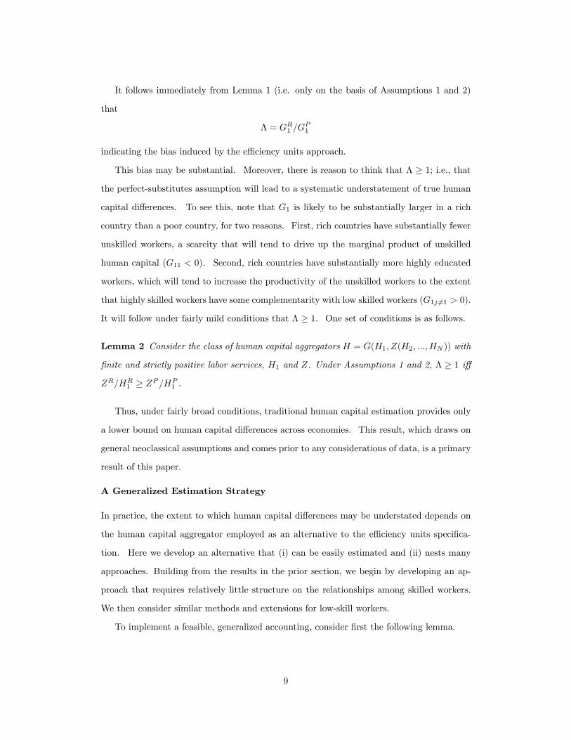
It follows immediately from Lemma 1 (i.e. only on the basis of Assumptions 1 and 2)
that
� = GR1 =GP1
indicating the bias induced by the e¢ ciency units approach.
This bias may be substantial. Moreover, there is reason to think that � � 1; i.e., that
the perfect-substitutes assumption will lead to a systematic understatement of true human
capital di¤erences. To see this, note that G1 is likely to be substantially larger in a rich
country than a poor country, for two reasons. First, rich countries have substantially fewer
unskilled workers, a scarcity that will tend to drive up the marginal product of unskilled
human capital (G11 < 0). Second, rich countries have substantially more highly educated
workers, which will tend to increase the productivity of the unskilled workers to the extent
that highly skilled workers have some complementarity with low skilled workers (G1j 6=1 > 0).
It will follow under fairly mild conditions that � � 1. One set of conditions is as follows.
Lemma 2 Consider the class of human capital aggregators H = G(H1; Z(H2; :::;HN )) with
�nite and strictly positive labor services, H1 and Z. Under Assumptions 1 and 2, � � 1 i¤
ZR=HR1 � ZP =HP
1 .
Thus, under fairly broad conditions, traditional human capital estimation provides only
a lower bound on human capital di¤erences across economies. This result, which draws on
general neoclassical assumptions and comes prior to any considerations of data, is a primary
result of this paper.
A Generalized Estimation Strategy
In practice, the extent to which human capital di¤erences may be understated depends on
the human capital aggregator employed as an alternative to the e¢ ciency units speci�ca-
tion. Here we develop an alternative that (i) can be easily estimated and (ii) nests many
approaches. Building from the results in the prior section, we begin by developing an ap-
proach that requires relatively little structure on the relationships among skilled workers.
We then consider similar methods and extensions for low-skill workers.
To implement a feasible, generalized accounting, consider �rst the following lemma.
9

Lemma 3 Consider the class of human capital aggregators H = G(H1; Z(H2; :::;HN )).
If such an aggregator can be inverted to write Z(H2; :::;HN ) = P (H;H1), then the human
capital stock can be estimated solely from information about H1, ~H, and production function
parameters.
This result suggests that there may be a broad class of aggregators that are relatively
easy to estimate, with the property that the aggregation of skilled labor, Z(H2;H3:::; HN ),
need not be measured directly. Moreover, any aggregator that meets the conditions of this
Lemma also meets the conditions of Lemma 2. Therefore, in comparison to traditional
human capital accounting, any such aggregator allows only greater human capital variation
across countries.
A �exible aggregator that satis�es the above conditions is as follows.
De�nition 3 De�ne the "Generalized Division of Labor" (GDL) aggregator as
H =hH
"�1"
1 + Z(H2;H3:::; HN )"�1"
i ""�1
(5)
where " 2 [0;1) is the elasticity of substitution between unskilled human capital, H1, and
an aggregation of all other human capital types, Z(H2;H3:::; HN ).
This aggregator encompasses, as special cases: (i) the traditional e¢ ciency-units aggre-
gator ~H =PN
i=1Hi, (ii) CES speci�cations, H" =�PN
i=1Hi"�1"
� ""�1, and (iii) the Jones
(2011) and Caselli and Coleman (2006) speci�cations, which assume an e¢ ciency-units ag-
gregation for higher skill classes, Z =PN
i=2Hi. More generally, the GDL aggregator
encompasses any constant-returns-to-scale aggregation Z(H2;H3:::; HN ). It incorporates
conceptually many possible types of labor division and interactions among skilled workers.
By Lemma 3, the aggregator (5) has the remarkably useful property that human capital
stocks can be estimated - identically - without specifying the form of Z(H2;H3:::; HN ).
Corollary 1 Under Assumptions 1 and 2, any human capital aggregator of the form (5) is
equivalently H = H1
1�"1
~H"
"�1 .
Therefore, the calculated human capital stock will be the same regardless of the underly-
ing structure of Z(H2;H3:::; HN ). By meeting the conditions of Lemma 3, we do not need
10

to know the potentially very complicated and di¢ cult to estimate form that this skilled
aggregator may take.
Given the Corollary, the implementation of the GDL aggregator becomes
HR
HP=hR1hP1
�LR1LP1
� 11�" ~LR1~LP1
! ""�1
(6)
In implementing this accounting, a simple way to proceed is to assume that workers have
the same innate skill, h1, across economies (Assumption 4 above). Then the accounting
can proceed from measures of L1, ~L1, and ". This generalized approach will be examined
empirically in Section II. We will see the possibility of substantial ampli�cation of human
capital variation so that, under some parameterizations, human capital may replace total
factor productivity residuals in accounting for cross-country income variation.
Additionally, one may also attempt to relax Assumption 4 and allow h1 to vary across
economies.6 To relax Assumption 4, one can draw on the insights of Hendricks (2002),
noting that immigration allows one to observe lower skilled workers from both a rich and
poor country in the same economy, thus controlling for broader economic di¤erences that
may otherwise cloud inferences about innate skill. Examining immigrants and native-born
workers in the rich economy, one may observe the wage ratio
wR1
wRjP1
=(@FR=@HR)GR1 h
R1
(@FR=@HR)GR1 hRjP1
=hR1
hRjP1
(7)
where wRjP1 and hRjP1 are the wage and skill of immigrants with little education working in
the rich country.
If the unskilled immigrants are a representative sample of the unskilled in the poor
country, then hRjP1 = hP1 . Therefore hR1 =hP1 = wR1 =w
RjP1 , which can be used in (6),
allowing estimation to proceed. Of course, one may imagine that unskilled immigrants
might not be representative of the source country�s low skilled population. If immigration
selects on higher ability among the unskilled in the source country, then hRjP1 > hP1 and
the co rrection wR1 =wRjP1 would then be conservative, providing a lower bound on human
capital di¤erences across countries.7
6For example, children in a rich country might have initial advantages (including better nutrition and/orother investments prior to starting school), suggesting hR1 > hP1 . On the other hand, those with littleschooling are a relatively small part of the population in rich countries, suggesting a possible selection e¤ect.If those with very little education in rich countries select on relatively low innate ability, than we mightimagine hR1 < h
P1 .
7Hendricks (2002) and Clemens (2011) review the extant literature and conclude that immigrant selection
11

Generalized Lower-Skill Services One may additionally consider more general ap-
proaches to measuring lower skill, depending on what kinds of workers are grouped as lower
skill and how one aggregates skills among these subgroups. For example, "lower skill" might
span from those with no education to those with high school education in some formula-
tions. Aggregation assumptions among these workers will naturally matter more as more
skill classes are grouped together.
Lower-skilled labor services can be de�ned generally as H1 = Q(H11;H12; :::;H1J) across
J sub-types of lower-skill workers. The perfect substitutes aggregation for the low-skilled
is then ~H1 = h11 ~L11, where ~L11 =PJ
j=1w1jw11L1j . To generalize in practice, one can
implement H1 =�H
��1�
11 +W (H12; :::;H1J)��1�
� ���1
, following the insights above. Coupled
with the aggregator (5), the accounting becomes
HR
HP=hR11hP11
LR11LP11
~LR11=L
R11
~LP11=LP11
! ���1
~LR1 =
~LR11~LP1 =
~LP11
! ""�1
(8)
providing a further generalization that additionally allows scarcity and complementarities to
operate across sub-groups of lower-skilled workers. In this further generalization, one may
again follow the traditional approach and assert that h11 does not vary across economies or,
alternatively, estimate it using wage data as above. The estimations in Section II consider
a range of approaches.
II. Empirical Estimation
Given the theoretical results, we now reconsider human capital variation and its capacity
to account for cross-country income variation. The analysis implements the generalized
aggregator developed in Section I.C and emphasizes comparison with the traditional special
case.
appears too mild to meaningfully a¤ect human capital accounting. The Data Appendix further reviewsthis literature and also presents analysis using state-of-the art microdata on Mexican immigration to theUnited States (Fernandez-Huertas Moraga 2011; Kaestner and Malamud, 2014), which con�rms modest ifany selection from the source population when looking at those with especially low education. Analysis ofworkers with somewhat more education also shows little evidence of selection, as further discussed in theData Appendix. See also the further discussion of immigration among skilled workers in Section II.D.
12

A. Data and Basic Measures
To facilitate comparison with the existing literature, we use the same data sets and ac-
counting methods in the review of Caselli (2005). Therefore any di¤erences between the
following analysis and the traditional conclusions are driven only by human capital aggre-
gation. Data on income per worker and investment are taken from the Penn World Tables
v6.1 (Heston, Summers, and Aten 2002) and data on educational attainment is taken from
Barro-Lee (2001). The physical capital stock is calculated using the perpetual inventory
method following Caselli (2005), and unskilled labor equivalents are calculated using data
on the wage return to schooling. These data are further described in the appendix.
Again following the standard literature, we will use Cobb-Douglas aggregation, Y =
K�(AH)1�� and take the capital share as � = 1=3. Writing YKH = K�H1�� to account
for the component of income explained by measurable factor inputs, Caselli (2005) de�nes
the success of a factors-only explanation as
success =Y RKH=Y
PKH
Y R=Y P
where R is a "rich" country and P is a "poor" country. We will denote the success measure
for traditional accounting, based on the e¢ ciency-units measure, ~H, as successT . The
relationship between the traditional success measure and the success measure for a general
human capital aggregator is
success = �1�� � successT
which follows from Lemma 1 and the de�nition of �.
[Insert Table 1 about here.]
B. Traditional Accounting
Table 1 Panel A summarizes standard data for development accounting. Comparing the
richest and poorest countries in the data (the USA and Congo-Kinshasa), the observed ratio
of income per-worker is 91. The capital ratio is larger, at 185, but the ratio of unskilled
labor equivalents, the traditional measure of human capital di¤erences, appears far more
modest, at 1:7. Comparing the 85th to 15th percentile (Israel and Kenya) or the 75th to
13

25th percentile (S. Korea and India), we again see that the ratio of income and physical
capital stocks is much greater than the ratio of unskilled labor equivalents.
Using unskilled labor equivalents to measure human capital stock variation, it follows
that successT = 45% comparing Korea and India, successT = 25% comparing Israel and
Kenya, and successT = 9% when comparing the USA to the Congo. These calculations
suggest that large residual productivity variation is needed to account for the wealth and
poverty of nations. These �ndings rely on unskilled labor equivalents, ~LR1 =~LP1 , to measure
human capital stock variation. Because unskilled labor equivalents vary little, human capital
appears to add little in accounting for income di¤erences.8
C. Generalized Accounting
Table 1 Panel B further summarizes additional data relevant to the generalized accounting.
While the variation in unskilled labor equivalents, ~LR1 =~LP1 , is modest in Table 1, the variation
in unskilled labor itself can be large. For example, individuals with no education appear
at approximately 1/5th the rate in Israel as they do in Kenya, and individuals with at least
some college education appear at 34 times the rate in Israel as they do in Kenya. Table
1 presents additional comparisons between S. Korea and India and between the U.S. and
Congo. Figure 2 presents labor allocation data for the full set of countries. In the presence
of aggregators that feature scarcity or complementarities, these large di¤erences in labor
allocations can be felt strongly.
[Insert Figure 2 about here.]
One Parameter Example
We �rst examine the single parameter model of (6). Unskilled workers are grouped as
those with completed primary education or less, which allows the skilled aggregator Z(:) to
encompass �exibly many higher-skilled categories. Table 2 (Panel A) reports the results of
such a generalized accounting, focusing on the Israel-Kenya example as an illustrative case.
The �rst row presents the human capital di¤erences, HR=HP , the second row presents the
ratio of these di¤erences to the traditional calculation, �GDL, and the third row presents
8Figure A1 shows successT when comparing all income percentiles from 70/30 (Malaysia/Honduras) to99/1 (USA-Congo). The average measure of successT is 31% over this sample.
14

the resulting success measure for capital inputs in accounting for cross-country income
di¤erences.
[Insert Table 2 about here.]
As shown in the table, factor-based explanations for income di¤erences are substan-
tially ampli�ed by allowing for di¤erentiated labor compared to the traditional case. As
complementarities across workers increase, the need for TFP residuals decline. For the
Israel-Kenya example, the need for residual TFP di¤erences is eliminated at " = 1:54,
where human capital di¤erences are HR=HP = 10:5.
Considering a broader set of rich-poor comparisons; for example, all country compar-
isons from the 70/30 income percentile (Malaysia/Honduras) up to the 99/1 percentile
(USA/Congo), we see similar large ampli�cations of human capital variation.9 Calculating
the elasticity of substitution, ", at which capital inputs can fully account for income di¤er-
ences shows that the mean value is " = 1:55 in this sample with a standard deviation of
0:34.
Table 2 (Panel B) further relaxes Assumption 4 and estimates hR1 =hP1 from immigrant
and native worker wage data. Examining the year 2000 U.S. Census, the mean wages of
employed unskilled workers varies modestly based on the source country (see Figure A2).
While the data are noisy, mean wages are about 17% lower for these unskilled workers
born in the U.S. compared to immigrants from the very poorest countries, which suggests
hR1 =hP1 � :83 (see Data Appendix for details).10 In practice, relaxing Assumption 4 has
modest e¤ects compared to relaxing Assumption 3, as seen in Table 2. Now residual TFP
di¤erences are eliminated when " = 1:50 for the Israel-Kenya comparison. Across the
broader set of rich-poor examples, additionally relaxing Assumption 4 leads to a mean value
of " = 1:58, with a standard deviation of 0:37.
Human capital stock estimations are presented for the broader sample in Figure 3. The
ratio of human stocks is shown for each pair of countries from the 70/30 income percentile
9The Malaysia/Honduras income ratio is 3.8. As income ratios (and capital measures) converge towards1, estimates of " become noisier.10This analysis makes wage comparisons among those with primary schooling or less, which is the rele-
vant approach for the delination between worker groups in this accounting implementation. Similar wagecorrections emerge when considering workers with somewhat more education, as discussed in the Data Ap-pendix. More generally, Table 2 suggests that much more action comes from relaxing the perfect substitutesassumption, which is the focus of the analysis.
15

to the 99/1 income percentile. Panel A considers the generalized framework, with " = 1:6.
Panel B considers traditional human capital accounting. We see that, as re�ected in Table
1, traditional human capital accounting admits very little human capital variation. It
appears orders of magnitude less than the variation in physical capital or income. With the
generalized framework human capital di¤erences substantially expand, admitting variation
similar in scale to the variation in income and physical capital.
[Insert Figure 3 about here.]
Two Parameter Example
In practice, grouping those with completed primary or less education encompasses those
with (i) completed primary education, (ii) some primary education, and (iii) no education
in the Barro-Lee data. To the extent that such workers may be substantially di¤erent in
practice (for example, those with completed primary education may be substantially more
literate and numerate than those with no education and thus engage in di¤erent tasks)
one may want to additionally consider more �exible aggregation across these subtypes. A
two parameter model can then be estimated, as in (8), where � additionally allows for
non-perfect-substitutes aggregation among lower skill workers.
Figure 4 (upper row) summarizes accounting results for the completed primary school
delineation when considering estimation across ("; �) space. The left panel presents the
mean ampli�cation � in human capital di¤erences across the rich-poor country pairs in
the sample. The right panel shows the mean success value across the rich-poor country
pairs. The generalized accounting again shows that human capital variation and the level
of success can be substantially elevated. Human capital di¤erences increase as either "
or � falls � i.e. as the estimation moves away from perfect substitutes. As imperfect
substitutability is introduced among the unskilled, the success measure reaches 100% at
higher levels of ".
In practice, with seven educational attainment levels de�ned in the Barro-Lee data, one
can consider numerous ways to delineate higher skilled and lower skilled workers in the
accounting implementation. Online Appendix I (Figures A1.1-A1.6) extensively explores
alternative de�nitions of the unskilled, including (i) all possible thresholds between skilled
and unskilled in the Barro-Lee data and (ii) �exible aggregation among the unskilled them-
16

selves. Here we feature two additional cases: grouping lower-skilled workers as those with
(a) some secondary or less education or (b) completed secondary or less education. Nat-
urally, as more of the seven Barro-Lee educational attainment categories are grouped as
lower-skill, the accounting becomes increasingly sensitive to how aggregation is performed
among these lower-skilled workers.11
[Insert Figure 4 about here.]
Figure 4 further summarizes analysis based on these delineations, showing the mean
ampli�cation � in human capital di¤erences and the mean success value across the rich-
poor country pairs. For example, with " = 1:5, one can now fully account for income
di¤erences with a mean value of � = 4:9 (middle row) and a mean value of � = 3:5 (lower
row). As with the primary schooling case, we again see substantial ampli�cation of human
capital variation and substantial elevation of success across a range of parameters, with
increased complementarities implying larger ampli�cation.
Parameter Discussion
The theoretical analysis of Section I.C presented broad neoclassical conditions under which
traditional accounting provides a lower bound on human capital variation across economies.
The generalized accounting above suggests substantial ampli�cation is possible, to the extent
that capital variation may potentially be large enough to fully account for the large income
variation across rich and poor countries.
Conclusive assessments of human capital variation depend partly on assessments of the
appropriate aggregator. Micro-evidence analyzing the elasticity of substitution between
skilled and unskilled labor typically suggests an elasticity in the [1; 2] interval with com-
mon estimates toward the center of this range.12 Perhaps the best-identi�ed estimate is
Ciccone and Peri (2005), who use compulsory schooling laws as a source of plausibly exoge-
nous variation in schooling across U.S. states and conclude that " � 1:5. These authors
grouped more educated workers as those with completed secondary education or above,
which corresponds most closely to the middle row of Figure 4. Using such an elasticity
in the generalized accounting would imply large ampli�cations of human capital variation.
11Shifting all worker types into the "lower skilled" category and aggregating them as perfect substituteswould of course return the accounting to the traditional case.12See, e.g. reviews in Katz and Autor (1999) and Ciccone and Peri (2005).
17

However, micro-evidence on the elasticity of substitution may apply poorly here for two rea-
sons. First, the main mass of research in the labor literature delineates workers as college
versus high-school educated (Ciccone and Peri (2005) is an exception) and more generally
does not allow for �exible aggregation within the skilled or unskilled groups. Second, the
microdata used in this literature comes from advanced economies and may not apply across
the larger labor-allocation di¤erences in the cross-country data.
The elasticity of substitution between worker types is traditionally inferred via OLS
regression (Katz and Autor (1999)) and regression can also be applied in the generalized
accounting context above. Such regressions demand substantial caveats given the identi�ca-
tion challenges, which include the potential for endogenous relationships between observed
and unobserved variables, measurement error, and multicollinearity problems. With such
important caveats in mind, illustrative regressions are presented for the interested reader in
Online Appendix I. Resulting estimates for " and � suggest that human capital di¤erences
across countries could be substantially ampli�ed, such that the success measure approaches
100%. However, the identi�cation challenges of such analysis, and their sensitivity, call
for substantial skepticism about such regression estimates, as discussed further in Online
Appendix I.
D. Discussion
This section considers intuitions and interpretations for the results and highlights open
issues. We draw out further reasoning that comes with di¤erentiated labor services as
compared to the perfect substitutes case.
Wages and Output with Di¤erentiated Labor Services
To develop additional intuition for the accounting results, it is useful to �rst consider the
distinction between wages and outputs that emerges when moving away from the perfect-
substitutes approach. In neoclassical theory the wage is a marginal revenue product, which
is the marginal product (in units of output) times that output�s price. Traditional account-
ing, in assuming perfect substitutes across labor types, turns o¤ relative price di¤erences
for di¤erent workers. Thus, it equates wage returns with skill returns. By contrast, the
generalized accounting allows for relative price di¤erences for di¤erentiated labor services
(see (3)). In short, the generalized approach introduces downward sloping demand.
18

To the extent that rich countries "�ood the market" with skilled labor compared to
unskilled labor, downward sloping demand implies that the relative price of skilled services
will decline. The more downward sloping the demand for skilled services, the greater the
relative price decline and hence the greater the output return to schooling in rich countries
needed to maintain the observed wage returns to schooling.13 This provides further intuition
for the generalized accounting. For example, as " decreases in Table 2, demand becomes
increasingly downward sloping. One correspondingly sees larger estimated di¤erences in
human capital services across countries. Online Appendix II provides speci�c estimates of
variation in skilled service outputs that are implied by accounting exercise, given the wage
and labor allocation data.
Immigration Outcomes with Di¤erentiated Labor Services
Within each economy, the wage returns, labor allocations, and estimated labor productiv-
ities are consistent in the accounting by construction. One may also ask what to expect
when moving workers across economies - i.e. via migration. With di¤erentiated labor
services, subtler issues arise than in the perfect substitutes case, because workers may now
productively shift occupations when they enter a new economic environment. Broad intu-
ition comes from comparative advantage applied to multiple tasks, where workers can shift
their task allocation depending on relevant prices in the relevant economy. For example, if
skilled workers in poor countries have very low quality in skilled services compared to skilled
workers in rich countries, these skilled immigrants may undertake lower-skilled tasks. A
concrete example is an immigrant engineer who drives a taxi. In practice, skilled immi-
grants to the US exhibit (1) occupational shifting into jobs that are typically performed by
those with less education and (2) wage penalties compared to U.S.-born skilled workers but
wages commensurate with those of less-educated U.S. workers, as shown in a companion
paper (Jones 2011). Jones (2011) develops a model that may explain these immigration
features while informing cross-country income di¤erences along the above lines.14
13This interpretation requires the elasticity of substitution between skilled and unskilled labor to be greaterthan one, as is consistent with external evidence. I maintain this assumption in the discussion.14 In particular, an immigrant engineer driving a taxi becomes a natural (equilibrium) task allocation
when the immigrant�s engineering skills are of substantially poorer quality than a US-trained engineer.With reallocation across tasks, the wage in the new economy re�ects not the worker�s source-country task atthe new-country price, but the worker�s new-country task at the new-country price. If low-skilled servicesare scarce in rich countries (so these services are priced relatively highly) while the immigrant has low qualityskill at the skilled task (which is abundant and thus priced relatively cheaply in the rich country) the skilledimmigrant can do better by downshifting on the occupational ladder upon migration. The capacity to
19

Heterogeneous Skill Returns with Di¤erentiated Labor Services
The generalized accounting, like the traditional case, infers the productivity gains from
human capital investment building from evidence on the wage returns to schooling. An
additional interpretative question is to ask whether the wage gains associated with more
schooling are in fact due to human capital investment as opposed to simply being associ-
ated with it. This identi�cation challenge, if left unchecked, would undermine the basis for
accounting (generalized or traditional), and it raises additional interpretative questions con-
cerning the link between human capital investments and other features, such as skill-biased
technology residuals.
One can narrow interpretations by considering the large IV literature on the returns to
schooling, which is intended to make causative assessments of schooling investments. The
IV literature suggests an extra year of schooling raises wages by approximately 10%, which
has been shown in both rich and poor countries (see, e.g., the review by Card (2003)). This
literature provides an empirical basis for going beyond the identi�cation problem, so that
the returns to schooling can be interpreted causatively as the treatment of schooling itself.
Given such wage evidence, what the generalized accounting e¤ectively does, by considering
di¤erentiated labor services, is to add downward sloping demand to the interpretation of
those IV wage returns.
Of course, the interesting additional implication is that one also interprets much greater
impact of schooling on output in rich countries than in poor countries. In rich countries, a
10% gain in wages requires a relatively large increase in output, given the abundant supply of
skilled labor depressing the relative prices of skilled services. By contrast, in poor countries,
a similar wage gain is supported with a much smaller increase in skilled outputs, given the
relative scarcity of skilled workers. Bringing the generalized accounting together with the
IV literature thus suggests two points: (1) human capital investment appears causative but
(2) its e¤ects are highly heterogeneous.
Such heterogeneous treatment e¤ects suggest substantial care in assessing human capital
policy. While policy statements go beyond the purpose of this paper, the following thought
reallocate thus helps the immigrant achieve a higher real wage than they otherwise would, and the marginalrevenue product at the lower skilled tasks (e.g. retail services, taxi services, etc) provides a lower bound onthe wage the immigrant can earn. This wage can also be substantially higher than the skilled wage theskilled worker leaves behind, if that worker comes from a poor country. See Jones (2011) for theory andevidence.
20

experiment may be clarifying. Given the generalized accounting, it would appear that reduc-
ing human capital stocks in the U.S. to the levels in the Congo (which would require taking
virtually all college-educated workers and most secondary-educated workers throughout all
sectors of the economy and replacing them with workers who have no education at all) would
cause the U.S. to experience a precipitous drop in output. This outcome is very di¤erent
than what traditional accounting allows. However, giving workers in the Congo the U.S.
distribution of educational duration (coupled with appropriate physical capital deepening)
does not necessarily imply that Congolese real income would rise to U.S. levels. In fact, �x-
ing the current quality of skilled workers in the Congo, producing more such workers might
be counterproductive. Thus, even as the generalized accounting may bring human capital
toward the center of the development picture, simply increasing the quantity of education in
poor countries may not be a well motivated implication. Heterogeneous treatment e¤ects
suggest that education policy choices require more subtle understanding, where the quality
of investment may be key and where the success of educational investments may interact
with other economic and institutional features.15
III. Conclusion
Human capital accounting operates under the assumption that the productivity advantage
of human capital can be inferred by comparing the productivity of those with more human
capital with those with less human capital. In practice, this productivity comparison is
traditionally made using relative wages: all types of workers in an economy are translated
into �unskilled equivalents�, with weights based on the wage gains associated with higher
skill (e.g. Klenow and Rodriguez-Clare 1997, Hall and Jones 1999, Caselli 2005). Using this
approach to construct human capital stocks, the literature �nds that human capital variation
across countries is small, accounting for no more than a small portion of the di¤erences in
per-capita income across countries. This in�uential conclusion suggests that human capital
investments can play at most a modest role in economic development.
This paper continues within the broad paradigm of human capital accounting, where the
productivity advantage of human capital is inferred by comparing workers with more or less
15Online Appendix II further explores labor di¤erentiation among skilled workers, linking human capitalinvestment, ideas, and institutions to provide a candidate explanation for large quality di¤erences of skillworkers across economies that can match the accounting �ndings.
21

human capital. By generalizing the method to a broad class of human capital aggregators,
however, the paper reaches three conclusions. First, the productivity gains associated with
human capital investments cannot reveal themselves through relative wages alone unless
workers are perfect substitutes. Second, the perfect substitutes accounting will understate
the variation in human capital across countries under broad conditions. Third, a generalized
empirical exercise suggests that human capital variation can possibly account for the large
income di¤erences across countries.
The theoretical results in this paper provide broad conditions under which traditional
human capital measurement, by ignoring complementarities and scarcity among human
capital types, would understate human capital variation, suggesting important areas for
further research, including a re�ned understanding of the sources of human capital quality.
While the framework is illustrated here using cross-country income di¤erences, the same
framework has other natural applications at the level of countries, regions, cities, or �rms.
Growth accounting provides one direction for future work, as do �rm-level productivity
studies. The urban economics and agglomeration literatures are another direction, where
productivity gains from labor di¤erentiation are often suggested but will not be captured
using traditional human capital measures.
22

Appendix
Proof of Lemma 1
Proof. H = G(H1;H2; :::;HN ) is constant returns in its inputs (Assumption 1). Therefore,
by Euler�s theorem for homogeneous functions, the true human capital aggregate can gener-
ically be written H =PN
i=1GiHi. Rewrite this expression as H = G1h1PN
i=1GihiG1h1
Li.
Recalling that wi = @F@HGihi (Assumption 2), so that
wiw1= Gihi
G1h1, we can therefore write
H = G1h1 ~L1, where ~L1 =PN
i=1wiw1Li.
Proof of Lemma 2
Proof. If H = G(H1; Z) is constant returns to scale, then G1 is homogeneous of degree
zero by Euler�s theorem. Therefore G1(H1; Z) = G1(H1=Z; 1). Noting that G11 � 0, it
follows that � = GR1 =GP1 � 1 i¤ ZR=HR
1 � ZP =HP1 .
Proof of Lemma 3
Proof. By Lemma 1, H = G1 ~H, providing an independent expression for H based
on its �rst derivative. If the human capital aggregator can be manipulated into the
form H = V (H1; Z(H2; :::;HN )) = V (H1; P (H;H1)), then we have from Lemma 1 H =
V1(H1; P (H;H1)) ~H. This provides an implicit function determining H solely as a function
of H1 and ~H; that is, without reference to Z(H2; :::;HN ).
Proof of Corollary 1
Proof. By Lemma 1, H = G1 ~H. For the GDL aggregator, G1 = (H=H1)1" . Thus H =
H1
1�"1
~H"
"�1 .
Data AppendixCapital Stocks
To minimize sources of di¤erence with standard assessments, this paper uses the same
data in Caselli�s (2005) review of cross-country income accounting. Income per worker
is taken from the Penn World Tables v6.1 (Heston, Summers, and Aten 2002) and uses
the 1996 benchmark year. Capital per worker is calculated using the perpetual inventory
23

method, Kt = It+(1� �)Kt�1, where the depreciation rate is set to � = 0:06 and the initial
capital stock is estimated as K0 = I0=(g + �). Further details are given in Section 2.1
of Caselli (2005). As a robustness check, I have also considered calculating capital stocks
as the equilibrium value under Assumptions 1 and 2 with a Cobb-Douglas aggregator; i.e.,
K = (�=r)Y , where � = 1=3 is the capital share and r = 0:1. This alternative method
provides similar results as in the main paper.
To calculate human capital stocks, I use Barro and Lee (2001) for the labor supply
quantities for those at least 25 years of age, which are provided in seven groups: no schooling,
some primary, completed primary, some secondary, completed secondary, some tertiary, and
completed tertiary. Schooling duration for primary and secondary workers are taken from
Caselli and Coleman (2006) and schooling duration for completed tertiary is assumed to be
4 years. Schooling duration for "some" education in a category is assumed to be half the
duration for complete education in that category. Figure 2 summarizes the Barro and Lee
labor allocation data.
For wage returns to schooling, I use Mincerian coe¢ cients from Psacharopoulos (1994)
as interpreted by Caselli (2005). Let s be the years of schooling and let relative wages be
w(s) = w(0)e�s. Psacharopoulos (1994) �nds that wage returns per year of schooling are
higher in poorer countries, and Caselli summarizes these �ndings with the following rule.
Let � = 0:13 for countries with �s � 4, where �s = (1=L)PN
i=1 siLi is the country�s average
years schooling. Meanwhile, let � = 0:10 for countries with 4 < �s � 8, and let � = 0:07 for
the most educated countries with �s > 8. Unskilled labor equivalents are then calculated as
~L1 =PN
i=1 e�siLi in each country.
As a robustness check, I have considered calculating ~H under a variety of other assump-
tions. The results using the GDL aggregators are broadly robust to reasonable alternatives.
For example, if we set � = :10 (the global average) for all countries, then the gap between
unskilled labor equivalents widens slightly, since the returns to education in poor countries
now appear lower and the returns in rich countries appear higher. The resulting increase
in human capital ratio means that capital inputs can fully account for income di¤erences at
somewhat higher values of the elasticity of substitution between the higher and lower skill
workers.
[Insert Figure A1 about here.]
24

Variation in the Quality of Unskilled Labor
Following the theoretical analysis in Section I.C, the di¤erence in unskilled qualities are
estimated as hR1 =hP1 = wR1 =w
RjP1 , where wages are for unskilled workers in the U.S. The
term wR1 is the mean wage for unskilled workers born in the US and wRjP1 is the mean wage
for unskilled workers born in a poor country and working in the US.
Wages are calculated from the 5% microsample of the 2000 U.S. Census (available from
www.ipums.org, Ruggles et al. (2010)). Unskilled workers are de�ned in the primary
analysis as employed individuals with 4 or less years of primary education (individuals with
educ=1 in the pums data set, which is the lowest schooling-duration group available) who
are between the ages of 20 and 65. To facilitate comparisons, mean wages are calculated for
individuals who speak English well (individuals with speakeng=3, 4, or 5 in the pums data
set).
Figure A2 presents the data, with the mean wage ratio, wRjP1 =wR1 , plotted against log
per-capita income of the source country. (National income data is taken from the Penn
World Tables v6.1.) There is one observation per source country, but the size of the marker
is scaled to the number of observed workers from that source country. The �gure plots the
results net of �xed e¤ects for gender and each integer age in the sample.
[Insert Figure A2 about here.]
For accounting and regression analysis when relaxing Assumption 4, the (weighted) mean
of wR1 =wRjP1 is calculated for �ve groups of immigrants based on quintiles of average schooling
duration in the source country. In practice, these corrections adjust hR1 =hP1 modestly when
departing from hR1 =hP1 = 1, with a range of 0:87 to 1:20 depending on the quintile. The age
and gender controlled data is used, although using the raw wage means produces similar
�ndings. The corrections for hR1 =hP1 are then applied to the human capital stock in each
country.
Alternatively, one may compare individuals with somewhat more education. For exam-
ple, one may consider workers who have completed 10th grade (educ=4 in the pums data
set), who represent a larger share of the U.S. workforce.16 Using this educational group, the16This comparison also relates more closely to the analysis of Ciccone and Peri (2005), who de�ned lower
skilled workers as high school dropouts. Ciccone and Peri (2005) provide a better-identi�ed estimate of theparameter ", suggesting " = 1:5, although their estimate is made in the U.S. context and may not apply incross-country data.
25

wage correction continues to adjust hR1 =hP1 modestly, and similarly to the primary schooling
case, with a range of 0:85 to 1:29 depending on the income quintile of the source country.
The wage method for estimating hR1 =hP1 operates under the additional premise that im-
migrant workers are representative of the source country population (hRjP1 � hP1 ). Views
on this issue can be drawn from a large existing literature on immigrant selection. Reviews
of this literature (Hendricks 2002, Clemens 2011) argue that immigrant selection appears
modest. Studies around the world of various source and host country pairs tend to show a
mix of modest negative selection (e.g. de Coulon and Piracha 2005; Ibarraran and Lubot-
sky 2007) and positive selection (e.g. Chiquiar and Hanson 2005; Brucker and Trubswetter
2007; Brucker and Defoort 2009, McKenzie, Gibson, and Stillman 2010), which is consistent
with the theoretical ambiguity of the matter (e.g. Borjas 1987, McKenzie and Rapoport
2007) and further suggests that there is no large, systematic departure from representative
sampling. Some authors argue that there may be tendency toward positive selection on
observables (e.g. Hanson 2010), which may extend into unobservables (e.g. McKenzie, Gib-
son, and Stillman 2010), in which case the wage adjustment is conservative, providing a
lower bound on human capital di¤erences across countries.
While several studies examine populations with low average educational attainment,
none to my knowledge explicitly examine the category with four or less years of schooling,
which is the group used for the wage adjustment in this paper. I therefore consider addi-
tional empirical analysis, examining Mexican migration to the United States. Given that
U.S. Census data is used for the wage correction and that Mexicans are the most common
immigrant population to the U.S., this population may be especially relevant for this pa-
per. Recent studies using state-of-the-art Mexican microdata �nd, in consonance with the
broader literature, modest degrees of selection and further a mixed direction of selection
with slight positive selection from rural areas and slight negative selection from urban areas
(Fernandez-Huertas Moraga 2011, 2013; Kaestner and Malamud 2014). To examine selec-
tion among those with four or less years of education, I have acquired both the Encuesta
Nacional de Empleo Trimestral sample used in Fernandez-Huertas Moraga (2011) and the
Mexican Family Life Survey sample used in Kaestner and Malamud (2014).17 Table A1
shows the results, examining the real earnings measures used in these studies and compar-
17See their papers for detailed description of the data and their earnings variables.
26

ing those who migrate to the U.S. with those who stay at home. The analysis �nds little
selection among migrants using either sample and regardless of age and gender controls.
Thus, on the basis of these data, the immigrant sample looks broadly representative.
[Insert Table A1 about here.]
Overall neither the wage correction using U.S. Census data nor extant evidence about
immigrant selection point to a substantial role for Assumption 4. One can use other
reasonable methods to calculate wR1 =wRjP1 and apply it to the human capital measures,
but in general the primary �ndings of the paper are robust to such variations, because the
implications of relaxing the perfect-substitutes assumption tend to be much greater.
References
[1] Barro, Robert J. and Jong-Wha Lee. �International Data on Educational Attainment:
Updates and Implications,�Oxford Economic Papers, 53 (3), 2001, 541-563.
[2] Borjas, George J. �Self-selection and the Earnings of Immigrants�, American Economic
Review, 77 (4), 1987, 531-53.
[3] Bowlus, Audra J. and Chris Robinson, "Human Capital Prices, Productivity, and
Growth," CLSRN Working Paper No. 89, 2011.
[4] Brucker, Herbert and Cecily Defoort. "Inequality and the Self-selection of International
Migrants: Theory and New Evidence," International Journal of Manpower, 30 (7),
2009, 742-764.
[5] Brucker, Herbert and Parvati Trubswetter. �Do the Best go West? An Analysis of
the Self-selection of Employed East-West Migrants in Germany�, Empirica, 34, 2007,
371-94.
[6] Card, David. "Estimating the Return to Schooling: Progress on Some Persistent
Econometric Problems," Econometrica, 69 (5), 2003, 1127-1160.
[7] Caselli, Francesco. "Accounting for Cross-Country Income Di¤erences", The Handbook
of Economic Growth, Aghion and Durlauf eds., Elsevier, 2005.
27

[8] Caselli, Francesco and Wilbur J. Coleman. "The World Technology Frontier", American
Economic Review, June 2006, 96 (3), 499-522.
[9] Chiquiar, Daniel and Gordon H. Hanson, �International Migration, Self-Selection, and
the Distribution of Wages: Evidence from Mexico and the United States,�Journal of
Political Economy, 113 (2), 2005, 239�281.
[10] Ciccone, Antonio and Giovanni Peri, "Long-Run Substitutability Between More and
Less Educated Workers: Evidence from U.S. States, 1950�1990," The Review of Eco-
nomics and Statistics, 87(4), 2005, 652-663.
[11] Clemens, Michael A. "Economics and Emigration: Trillion-Dollar Bills on the Side-
walk?" Journal of Economic Perspectives, Summer 2011, 25 (3), 83-106.
[12] Fernandez-Huertas Moraga, Jesus. "New Evidence on Emigrant Selection," The Review
of Economics and Statistics, February 2011, 93(1), 72-96.
[13] Fernandez-Huertas Moraga, Jesus. "Understanding Di¤erent Migrant Selection Pat-
terns in Rural and Urban Mexico," Mimeo FEDEA, 2013.
[14] Hall, Robert and Charles Jones. "Why Do Some Countries Produce So Much More
Output Per Worker Than Others?", Quarterly Journal of Economics, February 1999,
114 (1), 83-116.
[15] Hanson, Gordon H. "International Migration and the Developing World," Handbook of
Development Economics, Volume V, Chapter 66, 2010.
[16] Hendricks, Lutz. "How Important Is Human Capital for Development? Evidence from
Immigrant Earnings," American Economic Review, March 2002, 92 (1), 198-219.
[17] Heston, Alan, Robert Summers, and Bettina Aten. Penn World Tables Version 6.1.
Downloadable dataset. Center for International Comparisons at the University of Penn-
sylvania, 2002.
[18] Hsieh, Chang-Tai and Peter J. Klenow. "Development Accounting," American Eco-
nomic Journal: Macroeconomics, January 2010, 2 (1), 207-223.
28

[19] Ibarraran, Pablo and Darren Lubotsky. "Mexican Immigration and Self-Selection: New
Evidence from the 2000 Mexican Census," Mexican Immigration to the United States,
Chapter 5, George J. Borjas (ed.), 2007
[20] Jones, Benjamin F. "The Knowledge Trap: Human Capital and Development Recon-
sidered", NBER Working Paper #14138 and Northwestern University mimeo, 2011.
[21] Kaestner, Robert and Ofer Malamud, "Self-Selection and International Migration: New
Evidence from Mexico," The Review of Economics and Statistics, 2014, 96 (1), 78-91.
[22] Katz, Lawrence F. and David H. Autor, "Changes in the Wage Structure and Earnings
Inequality," Handbook of Labor Economics Volume 3 Chapter 26, 1999, 1463-1555.
[23] Klenow, Peter J., and Andres Rodriguez-Clare, �The Neoclassical Revival in Growth
Economics: Has It Gone Too Far?�, in: B.S. Bernanke, and J.J. Rotemberg, eds.,
NBER Macroeconomics Annual (MIT Press, Cambridge), 1997, 73-103.
[24] Mankiw, N. Gregory, David Romer and David N. Weil. "A Contribution to the Empirics
of Economic Growth", Quarterly Journal of Economics, May 1992, 107 (2), 407-437
[25] McKenzie, David and Hillel Rapoport. �Network e¤ects and the dynamics of migra-
tion and inequality: Theory and evidence from Mexico.�Journal of Development Eco-
nomics, 8, 2007, 1�24.
[26] McKenzie, David, John Gibson, and Steven Stillman. �How Important Is Selection?
Experimental vs. Non-experimental Measures of the Income Gains from Migration,�
Journal of the European Economic Association, 8 (4), 2010, 913�45.
[27] Psacharopoulos, George. "Returns to Investment in Education: A Global Update",
World Development, 1994, 22 (9), 1325-43.
[28] Ruggles, Steven J. Trent Alexander, Katie Genadek, Ronald Goeken, Matthew B.
Schroeder, and Matthew Sobek. Integrated Public Use Microdata Series: Version 5.0
[Machine-readable database]. Minneapolis: University of Minnesota, 2010.
29

30
Table 1: Basic Data
Rich v Poor
Measure
99th / 1st Percentile
(USA/Zaire)
85th / 15th Percentile
(Israel/Kenya)
75th / 25th Percentile
(S Korea/India)
Panel A: Traditional Accounting Measures
PR YY / (Income)
90.9 16.9 6.3
pR KK / (Capital stock)
185.3 43.9 17.4
PR LL 11
~/
~
(Unskilled worker equivalents) 1.70 1.33 1.15
Traditional Success 9% 25% 45%
Panel B: Relative Labor Allocations
Lab
or R
atio
s
(Ric
h / P
oor)
No Education .02 .21 .23
Some or Completed Primary
.23 .78 1.71
Some or Completed High School
11.7 6.7 3.4
Some or Completed College
56.2 34.3 3.2
Income and capital stock measures are per worker. Relative labor allocations are the population percentage of a given educational type in the rich country as a ratio to the corresponding
percentage for the poor country. Populations percentages are for those over age 25. Data sources and methods are further described in the text and appendix.

31
Table 2: Human Capital and Income: Generalized Accounting
Elasticity of Substitution Between Unskilled Labor, H1, and Skilled Aggregate, Z(H2,..,HN)
1 1.2 1.4 1.6 1.8 2.0 ∞
Panel A: Relaxing Assumption 3
HR/ HP ∞ 358 21.9 8.6 5.4 4.1 1.3
Λ ∞ 269 16.4 6.5 4.0 3.1 1
Success ∞ 1050% 163% 88% 64% 54% 25%
Panel B: Relaxing Assumptions 3 and 4
HR/ HP ∞ 306 18.6 7.3 4.6 3.5 1.1
Λ ∞ 269 16.4 6.5 4.0 3.1 1
Success ∞ 950% 147% 79% 58% 48% 23%
This table compares Israel and Kenya, which represent the 85th and 15th percentile countries respectively ranked by income per worker. HR/ HP is the ratio of human capital stocks. Λ is the ratio of HR/ HP at the indicated elasticity of substitution to HR/ HP for the infinite elasticity of substitution case. Success is the consequent percentage of the income variation that is explained by variation in
capital inputs. Figure 2 summarizes accounting for a broader set of rich and poor countries and shows that Israel and Kenya provide a useful benchmark, as discussed in the text.

32
Figure 1: Income per Worker and Mean Schooling Duration
Figure 2: Fraction of Workers with Given Schooling
ARG
AUS
AUT
BEL
BEN
BGDBOL
BRA
BRB
BWA
CAF
CANCHE
CHL
CHN
CMR
COG
COL CRI
CYP
DNK
DOM
DZA
ECU
EGY
ESPFIN
FJI
FRAGBR
GHAGMB
GRC
GTM
GUY
HKG
HND
HTI
HUN
IDN
IND
IRL
IRN
ISLISR
ITA
JAM
JOR
JPN
KEN
KOR
LKA
LSO
MEX
MLIMOZ
MUS
MWI
MYS
NER
NIC
NLDNOR
NZL
PAK
PANPER
PHL
PNG
PRT
PRY
ROM
RWA
SEN
SGP
SLE
SLV
SWE
SYR
TGO
THA
TTO
TUN TUR
UGA
URY
USA
VEN
ZAF
ZAR
ZMB
ZWE
1000
2000
4000
8000
1600
032
000
Inco
me
Per
Wor
ker
(log
scal
e)
0 2 4 6 8 10 12Mean Years of Schooling
ARGAUSAUTBEL
BEN
BGD
BOL
BRA
BRB
BWA
CAF
CANCHE
CHL
CHN
CMR COG
COL
CRI
CYPDEUDNK
DOM
DZA
ECU
EGY
ESPFIN
FJI
FRAGBR
GHA
GMB
GRC
GTM
GUY
HKG
HND
HTI
HUN
IDN
IND
IRL
IRN
ISL
ISRITA
JAM
JOR
JPN
KEN
KORLKA
LSO MEX
MLI
MOZ
MUS
MWI
MYS
NER
NIC
NLDNORNZL
PAK
PANPER
PHL
PNG
PRT
PRYROM
RWASEN
SGP
SLE
SLV
SWE
SYR
TGO
THA
TTO
TUN
TUR
UGA
URYUSA
VENZAF
ZAR
ZMBZWE
020
4060
8010
0N
o E
duca
tion
(%)
7 8 9 10 11Log of Income Per Worker (PPP)
ARG
AUS
AUT
BEL
BEN
BGD
BOL
BRABRB
BWA
CAF CAN
CHE
CHL
CHNCMR
COG
COL
CRI
CYP
DEU
DNKDOM
DZA
ECU
EGY
ESP
FINFJI
FRA
GBR
GHA
GMB
GRC
GTM
GUY
HKG
HND
HTI
HUN
IDN
IND
IRL
IRN
ISL
ISR
ITA
JAM
JOR
JPNKEN
KOR
LKA
LSO
MEX
MLI
MOZ
MUS
MWIMYS
NER
NIC
NLD
NOR
NZLPAK
PANPER
PHL
PNG
PRT
PRY
ROM
RWASEN
SGP
SLE
SLV
SWE
SYR
TGO
THA TTO
TUN
TUR
UGA
URY
USA
VENZAF
ZAR
ZMB
ZWE
020
4060
80S
ome
or C
ompl
ete
Pri
mar
y (%
)
7 8 9 10 11Log of Income Per Worker (PPP)
ARG
AUSAUT
BEL
BEN
BGDBOL
BRA
BRB
BWACAF
CAN
CHE
CHLCHN
CMR
COG COL
CRI
CYP
DEU
DNK
DOM
DZA
ECUEGY
ESP
FIN
FJI FRA
GBR
GHA
GMB
GRC
GTM
GUY
HKG
HNDHTI
HUN
IDNIND
IRL
IRN
ISLISR
ITA
JAM
JOR
JPN
KEN
KOR
LKA
LSO
MEX
MLIMOZ
MUS
MWI
MYS
NERNIC
NLD
NOR
NZL
PAK
PANPERPHL
PNG
PRTPRY
ROM
RWASEN
SGP
SLESLV
SWE
SYRTGOTHA
TTO
TUNTUR
UGA
URY
USA
VEN
ZAF
ZAR
ZMB
ZWE
020
4060
Som
e or
Com
plet
e S
econ
dary
(%
)
7 8 9 10 11Log of Income Per Worker (PPP)
ARG
AUS
AUT
BEL
BENBGD
BOLBRABRB
BWACAF
CAN
CHE
CHL
CHNCMRCOG
COL
CRICYP
DEU
DNK
DOM
DZA
ECU
EGYESP
FIN
FJI
FRAGBR
GHAGMB
GRC
GTMGUY
HKG
HNDHTI
HUN
IDN
IND
IRL
IRN
ISL
ISR
ITA
JAM
JOR
JPN
KEN
KOR
LKALSO
MEX
MLIMOZ
MUSMWI
MYSNER
NIC
NLDNOR
NZL
PAK
PANPER
PHL
PNG
PRTPRYROM
RWA SEN
SGP
SLE
SLV
SWE
SYR
TGO
THATTOTUN
TUR
UGA
URY
USA
VEN
ZAFZAR ZMBZWE0
1020
3040
Som
e or
Com
plet
e T
ertia
ry (
%)
7 8 9 10 11Log of Income Per Worker (PPP)

33
Figure 3: Human Capital Stock Variation
Panel A: Generalized Human Capital Stock
Panel B: Traditional Human Capital Stock
USA/ZAR
HKG/NERITA/RWA
BEL/MWI
NOR/MLI
IRL/MOZ
AUS/UGA
NLD/CAF
AUT/TGO
CAN/GMB
FRA/BEN
DNK/ZMB
CHE/SLE
ISR/KEN
SGP/GHA
GBR/LSO
SWE/NPL
FIN/SEN
ISL/COG
ESP/CMR
JPN/HTI
NZL/CHN
KOR/INDCYP/NICGRC/ZWE
PRT/BGDBRB/BOL
MYS/HND
12
48
1632
6412
8G
ener
aliz
ed H
uman
Cap
ital S
tock
Rat
io (
log
scal
e)
5 10 20 40 80Income Ratio (log scale)
USA/ZARHKG/NERITA/RWA
BEL/MWINOR/MLIIRL/MOZAUS/UGANLD/CAFAUT/TGOCAN/GMBFRA/BEN
DNK/ZMBCHE/SLE
ISR/KENSGP/GHAGBR/LSO
SWE/NPLFIN/SEN
ISL/COG
ESP/CMR
JPN/HTINZL/CHN
KOR/INDCYP/NIC
GRC/ZWEPRT/BGD
BRB/BOLMYS/HND12
48
1632
6412
8T
radi
tiona
l Hum
an C
apita
l Sto
ck R
atio
(lo
g sc
ale)
5 10 20 40 80Income Ratio (log scale)

34
Figure 4: Generalized Accounting with Two Parameters
Λ (amplification factor) Success (% income variation)
Notes: Generalized accounting is considered for different delineations between higher skill and lower skill groups. The lower skill group is alternatively defined as those with completed primary or less education (top row), some
secondary or less education (middle row), and completed secondary or less education (bottom row). The amplification factor is the ratio of the generalized human capital differences to the traditional perfect-substitutes
measure. Success is the percentage of cross-country income variation accounted for.
Low
er S
kill
Gro
up h
as C
ompl
eted
Pr
imar
y or
Les
s Sc
hool
ing
Low
er S
kill
Gro
up h
as S
ome
Seco
ndar
y or
Les
s Sc
hool
ing
Low
er S
kill
Gro
up h
as C
ompl
eted
Se
cond
ary
or L
ess
Scho
olin
g

35
Figure A1: Fraction of Income Difference Explained Using Traditional Human Capital Accounting
Figure A2: Wage Ratios from 2000 US Census among Employed Workers with Four or Less Years of Schooling, Conditional on Age and Gender
USA/ZAR
HKG/NERITA/RWA
BEL/MWINOR/MLI
IRL/MOZ
AUS/UGA
NLD/CAFAUT/TGO
CAN/GMBFRA/BEN
DNK/ZMB
CHE/SLE
ISR/KENSGP/GHA
GBR/LSO
SWE/NPLFIN/SEN
ISL/COG
ESP/CMR
JPN/HTI
NZL/CHN
KOR/IND
CYP/NIC
GRC/ZWEPRT/BGD
BRB/BOL
MYS/HND
0.2
.4.6
.81
Suc
cess
of T
radi
tiona
l Acc
ount
ing
5 10 20 40 80Income Ratio (log scale)
0.5
11.
52
Wag
e R
atio
to U
S W
orke
rs (
Uns
kille
d)
8 9 10 11Log Per-Capita Income

36
Table A1: Immigrant Selection, Four or Less Years of Schooling Dependent variable: log earnings (1) (2) (3) (4) (5) (6) (7) (8) All Rural Urban All All Rural Urban All Migrated to U.S.
-0.0240 0.167*** 0.0514 0.00875 0.00931 0.0880 -0.0174 -0.109
(0.0290) (0.0459) (0.0325) (0.0276) (0.167) (0.212) (0.258) (0.158) Controls(a) No No No Yes No No No Yes Data ENET ENET ENET ENET MxFLS MxFLS MxFLS MxFLS Observations 429,815 120,633 309,182 429,815 2,253 1,291 962 2,251 R-squared 0.000 0.000 0.000 0.163 0.000 0.000 0.000 0.126 Notes: (a)Controls include fixed effects for each age in years and dummies for gender and rural residency. I thank Jesus Fernandez-Huertas Moraga and Ofer Malamud for providing access to and guidance on the Encuesta Nacional de Empleo Trimestral (ENET) data and the Mexican Family Life Survey (MxFLS) data, and for sharing their constructed variables. For ENET, earnings are the real hourly wage. For MxFLS, the earnings are real annual earnings, including benefits and income from secondary jobs. Robust standard errors in parentheses *** p<0.01, ** p<0.05, * p<0.1

The Human Capital Stock: A Generalized ApproachOnline Appendices
Benjamin F. Jones�
May 2014
1 Online Appendix I: Further Human Capital StockAnalysis
This appendix presents additional calculations of human capital stocks. We further extend
the estimations presented in the main text by considering all possible delineations between
skilled and unskilled groups. We use the generalized, two-parameter human capital stock
developed in the main text
H = h11L11
�~L11=L11
� ���1
(~L1=~L11)"
"�1 (1)
where L11 is the mass of the least skilled category, h11 is their innate skill, ~L11 is a perfect
substitutes aggregation among the unskilled, and ~L1 is the traditional perfect substitutes
aggregation of all skill classes. Note that as �!1 and "!1, we return to the standard
perfect substitutes calculation used in traditional accounting.
To implement the accounting, we have
HR
HP=hR11hP11
LR11LP11
~LR11=L
R11
~LP11=LP11
! ���1
~LR1 =
~LR11~LP1 =
~LP11
! ""�1
Related, recall the de�nition � from the main text, measuring the ratio of generalized human
capital di¤erences to the traditional perfect-substitutes calculation. The ampli�cation of
human capital di¤erences is
� =LR11LP11
~LR1 =L
R11
~LP1 =LP11
! ���1
~LR1 =
~LR11~LP1 =
~LP11
! ""�1 ~LP1
~LR1
�Kellogg School of Management and NBER. Contact: 2001 Sheridan Road, Evanston IL 60208. Email:[email protected].
1

Similarly, recall that the metric success, which measures the percentage of cross-country
output variation predicted by variation in capital inputs, is
success = �1�� � successT
where successT is the success percentage under traditional accounting. These measures can
be calculated for any particular rich-poor country pair.
Figures A1.1-A1.6 present � and success across countries given various ("; �) pairs and
various delineations between unskilled and skilled workers. As in the main text, the measure
is calculated for all country pairs from the 70/30 to 99/1 percentiles in per-capita income.
The mean ampli�cation of human capital di¤erences and mean success rate across countries
is then presented for each set of parameters. Unskilled labor is de�ned using six di¤erent
delineations, using the �nest gradations available from the Barro-Lee data: (1) no schooling
(Figure A1.1); (2) some primary or less schooling (Figure A1.2); (3) completed primary
or less schooling (Figure A1.3); (4) some secondary or less schooling (Figure A1.4); (5)
completed secondary or less schooling (Figure A1.5); and (6) some tertiary or less schooling
(Figure A1.6). Cases (3)-(5) were featured in the text but are repeated here for ease of
comparison.
Several observations can be made. First, looking across these �gures, it is clear that the
generalized accounting substantially elevates human capital di¤erences and can help explain
cross-country income variation with much higher levels of success over a wide space of pa-
rameters and delineations between skilled and unskilled labor. Second, the human capital
ampli�cation increases as either � or " falls �that is, as we move away from perfect substi-
tutes. Third, higher cuto¤s between skilled and unskilled workers produce a given success
value at lower values of " and/or �. Put another way, as we expand the unskilled category,
the success measure increasingly depends on �. This �nding is natural: treating workers
as perfect substitutes diminishes human capital variation and, as we move more workers
into the unskilled category, how we treat these workers increasingly matters. Broadly,
we see that the capacity to substantially expand the role of human capital in development
accounting appears regardless of the skill cuto¤.
2
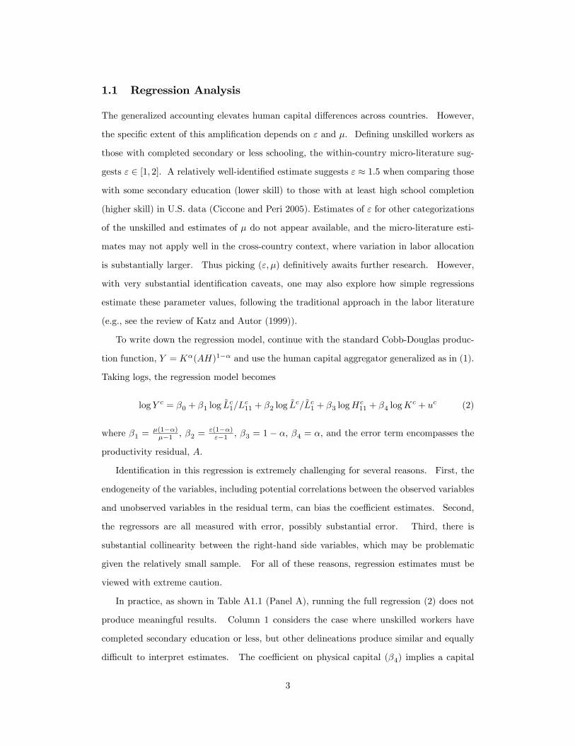
1.1 Regression Analysis
The generalized accounting elevates human capital di¤erences across countries. However,
the speci�c extent of this ampli�cation depends on " and �. De�ning unskilled workers as
those with completed secondary or less schooling, the within-country micro-literature sug-
gests " 2 [1; 2]. A relatively well-identi�ed estimate suggests " � 1:5 when comparing those
with some secondary education (lower skill) to those with at least high school completion
(higher skill) in U.S. data (Ciccone and Peri 2005). Estimates of " for other categorizations
of the unskilled and estimates of � do not appear available, and the micro-literature esti-
mates may not apply well in the cross-country context, where variation in labor allocation
is substantially larger. Thus picking ("; �) de�nitively awaits further research. However,
with very substantial identi�cation caveats, one may also explore how simple regressions
estimate these parameter values, following the traditional approach in the labor literature
(e.g., see the review of Katz and Autor (1999)).
To write down the regression model, continue with the standard Cobb-Douglas produc-
tion function, Y = K�(AH)1�� and use the human capital aggregator generalized as in (1).
Taking logs, the regression model becomes
log Y c = �0 + �1 log ~Lc1=L
c11 + �2 log ~L
c=~Lc1 + �3 logHc11 + �4 logK
c + uc (2)
where �1 =�(1��)��1 , �2 =
"(1��)"�1 , �3 = 1� �, �4 = �, and the error term encompasses the
productivity residual, A.
Identi�cation in this regression is extremely challenging for several reasons. First, the
endogeneity of the variables, including potential correlations between the observed variables
and unobserved variables in the residual term, can bias the coe¢ cient estimates. Second,
the regressors are all measured with error, possibly substantial error. Third, there is
substantial collinearity between the right-hand side variables, which may be problematic
given the relatively small sample. For all of these reasons, regression estimates must be
viewed with extreme caution.
In practice, as shown in Table A1.1 (Panel A), running the full regression (2) does not
produce meaningful results. Column 1 considers the case where unskilled workers have
completed secondary education or less, but other delineations produce similar and equally
di¢ cult to interpret estimates. The coe¢ cient on physical capital (�4) implies a capital
3

share (�) of approximately 0:69, while the coe¢ cient �3 provides a noisy estimate of � that
is substantially greater than 1. These values of � are neither consistent with each other1
nor consistent with well-known estimates of the capital share, which suggest that � is about
1=3 (e.g. Gollin 2002, Bernanke & Gurkaynak 2002). Moreover, the implied estimates of
" and � are ambiguous because � is unclear.2 The full regression model thus appears
uninformative of actual parameter values. As shown in column 2, regressing of logK on
the other explanatory variables produces an R2 of 0:82, suggestive of collinearity problems
(and the possibility of endogenous relationships between these variables). One way forward
with such regressions, as often used with collinearity problems, is to assert the parameters
we think are known from other literature. Namely, one may take the usual view that
� = 1=3, which implies the values of �3 and �4, and run the constrained regression.
With substantial caution given the identi�cation challenges, these results are presented
in Table A1.1 (Panel B). Each column considers a di¤erent delineation between skilled
and unskilled workers, and the implied values for " and � are presented in the �nal rows.
These speci�cations produce several observations. First, raising the threshold between
unskilled and skilled workers produces lower estimates of ". This �nding would suggest that
complementarities between skilled and unskilled workers appear greatest when we isolate
the very highly skilled. Second, looking at column 5, which corresponds to the secondary
versus tertiary schooling delineation in the extant micro-literature, we see " = 1:5, which is
similar to that literature�s estimates. Third, the point estimates show a higher elasticity of
substitution among unskilled workers, with � � 4 being typical. This �nding would suggest
that unskilled workers are more substitutable among themselves than they are with skilled
workers.
A slightly relaxed version of the constrained regression is presented in Table A1.1 (Panel
C). Here we continue to constrain the role of physical capital, with �4 = 1=3, but now let
�3 be estimated by the regression. As shown in the table, the estimates for " and � appear
broadly similar with this additional �exibility as in the regressions of Panel B, and these
regressions continue to estimate " = 1:5 using the completed secondary delineation. Inter-
estingly, the estimates for �3 are now statistically consistent with its theoretical condition
(�3 = 1� �), giving plausible values for the capital share.1A formal test strongly rejects the restriction �3 + �4 = 1.2These estimated parameters can be negative and thus also outside their theoretical constraints.
4

Lastly, and again with substantial caution required, Figure A1.7 takes the estimates of
the " and � from each regression (i.e. for each classi�cation of skilled workers) and examines
the relevant accounting calculations at these parameter values. In the upper panel of Figure
A1.7, we see that human capital di¤erences across country pairs would increase on average
by a factor of 3:4 to 7:1 depending on the delineation between skilled and unskilled workers.
The lower panel shows that the related success measure ranges from 72% to 109%. Thus,
across the possible delineations between skilled and unskilled workers, large ampli�cations
of human capital di¤erences would appear with, correspondingly, a capacity to account for
most or all of the income variation across countries.
5

2 Online Appendix II: Skilled Workers
A value of the human capital stock calculations in the text is that they do not require
detailed speci�cation of the aggregator and are robust to any constant-returns speci�cation
Z (H1;H2; :::;HN ). At the same time, it is useful to look "underneath the hood" and
gain a better understanding and intuition of where the variation in stocks may come from.
This Online Appendix proceeds in two parts. First, it explores variation in skill returns
across countries. As discussed in the paper, the productivity gains (in output) associated
with skill appear far larger in rich than poor countries. This appendix provides explicit
estimates of this variation and considers simple equilibrium reasoning to show why large
variation in skill returns across countries is consistent with modest variation in wage returns.
Second, this appendix examines a concrete explanation for the relatively enormous skill
returns in rich countries, emphasizing their greater collective acquisition of knowledge. This
approach, the "division of labor hypothesis", provides a candidate avenue for understanding
the heterogeneous treatment e¤ects of education across countries and draws a natural link
between human capital, institutions, ideas, and skill-bias.
2.1 Variation in Skilled Labor Services
Under Assumptions 1 and 2, the relative �ow of services for two groups of laborers in an
economy ishihj=wiwj
GjGi
(3)
as shown in the main text, where hi = Hi=Li is the mean �ow of services from the workers
in group i. Thus the relative service �ows (hi=hj), which are in units of output, can in
general be inferred from relative wages (wi=wj) and the relative prices of these intermediate
human capital services (Gj=Gi). Under traditional accounting, skill returns are mapped
purely from wage returns, because a perfect substitutes assumption turns o¤ considerations
of Gj=Gi. Under generalized accounting, one must also consider these relative prices.
In particular, with downward sloping demand, a relative abundance of skilled over un-
skilled services in rich countries will cause the relative price of skilled to unskilled services to
fall. In practice, skilled labor supply appears far higher in rich countries while wage returns
appear rather similar across countries. Figure A2.1 presents these data. De�ning lower
skilled workers as those with completed primary or less education, wage return variation is
6

tiny compared to labor supply variation. For example, the skilled labor allocation (LZ=L1)
is 2300% greater in Israel compared to Kenya, while the mean wage returns (wz=w1) are
only 20% lower. As another example, the skilled labor allocation is 17500% greater in the
USA compared to Congo, while mean wage returns are only 15% lower. With downward
sloping demand, and given these large di¤erences in labor allocations yet similar wage re-
turns, skilled workers in rich countries will therefore appear far more productive (in units
of output) than skilled workers in poor countries.
To estimate the variation in output gains associated with skill, we can again use the
human capital stock estimation approach of Section 3 in the paper. For example, using
the GDL aggregator in tandem with (3), one can infer the skilled-unskilled ratio of mean
service �ows ashRz =h
R1
hPz =hP1
=
�wRz =w
R1
wPz =wP1
� ""�1�LRz =L
R1
LPz =LP1
� 1"�1
(4)
where hz = Z(H2;H3:::; HN )=LZ is the mean �ow of services from skilled workers. That is,
the left hand side tells us the output gains from schooling in rich versus poor countries that
are implied by the generalized accounting. These are the output gains that are consistent
by construction, with the wage returns data, the labor allocation data, and the elasticity of
substitution parameter.
Table A2.1 (Panel A) reports the implied variation in hz=h1 for various values of the
parameter ", continuing with the rich-poor example in Table 2 of the main text. Recall that
human capital stock variation eliminates residual total factor productivity variation when
" � 1:6. At this value of ", the relative service �ows of skilled workers in the rich country
appear 98:6 times larger than in the poor country. This empirical �nding is consistent with
Caselli and Coleman (2006), but now explicitly extended to the general class of skilled labor
aggregators, Z(H2;H3:::; HN ). Thus similar wage returns are consistent with massive
di¤erences in labor allocation when skilled service �ows are substantially higher in rich
countries.
Skilled service �ows can be further articulated by specifying particular skilled aggrega-
tors, Z. For example, consider a sub-aggregator of skilled types
Z =
"NXi=2
H��1�
i
# ���1
(5)
where � is the elasticity of substitution among these types. Table A2.1 (Panel B) presents
7

the implied service �ows from these di¤erent groups of skilled workers.3 Taking a range of
� 2 [1:2; 2], the implied skill return advantages for skilled but less than tertiary-educated
workers in the rich country are in the interval [69; 103], while the skill returns among the
tertiary-educated are in the interval [60; 284]. In sum, the labor allocations and wage returns
evidence in Figure A2.1 are reconciled when service �ows from higher educated workers in
rich countries are far higher (as a group) than their service �ows in poor countries.
2.1.1 Further Intuition from Equilibrium Reasoning
To further interpret these �ndings, it is useful to consider why the world looks like Figure
A2.1, where there is little variation in wage returns across countries yet massive variation
in labor allocations. One straightforward interpretation lies in endogenous labor supply.
Simple endogenous labor supply models act to drive individuals�equilibrium wage returns
toward their discount rates (e.g. Willis 1986) as workers optimize their human capital in-
vestments. Namely, if wage returns to schooling were unusually high, then more individuals
would choose to become skilled, causing the relative prices of skilled services to fall and con-
straining wage gains. Thus endogenous labor supply can act to decouple equilibrium wage
returns from productivity considerations, and may thus help clarify why enormously di¤er-
ent skill returns across countries would appear through large di¤erences in labor allocations
but little di¤erence in wage returns.
To see this idea formally, consider a stylized theory where workers choose their education
level to maximize their income.
Assumption 1 Let individual income, y, as a function of educational duration, s, be
y(s; �) =R1sw(s; �)e�rtdt where � is an individual speci�c parameter. Let individuals
maximize income with respect to educational duration.
In this setting, the individual will choose a personally optimal level of education such
that@w=@s
w= r (6)
3The returns for the sub-groups of workers are calculated using (5) as
hi6=1h1
=
�wi
w1
� ���1
�Li
L1
� 1��1
�hZ
h1
LZ
L1
� ��""(��1)
The calculations in Panel B of Table A2.1 assume " = 1:6 in the GDL aggregator; i.e. the value of " wherecapital variation fully explains the income variation.
8

In other words, the individual�s wage return will be log-linear in educational duration at their
optimal schooling choice, with a return of r%.4 This log-linearity looks like a Mincerian
return. It is also independent of the mapping between skill and schooling. That is, the
individual�s wage return will settle here according to (6) regardless of how schooling and skill
map together. If more schooling brought wage gains above r for some individuals, these
individuals would naturally seek more education, causing the price of the higher-schooling
labor services to fall until each individual�s equilibrium wage return (6) returned to r. While
moving from individual wage returns to economy-wide wage returns requires some further
assumptions, it is clear that simple equilibrium reasoning constrains wage variation. Hence,
we may expect the limited wage return variation across countries seen in Figure A2.1, even
as skill returns can vary enormously. Thus wage returns can act to mask rather than reveal
variation in skill returns. This equilibrium reasoning provides an additional perspective on
the data. It also provides an additional perspective on the problem underlying traditional
human capital accounting, which assumes that wage returns on their own can guide human
capital inferences.
2.2 The Division of Labor
In advanced economies, and especially among the highly educated, skills appear highly
di¤erentiated. Skills appear to di¤er across medical doctors, chemical engineers, computer
scientists, molecular biologists, lawyers, and architects, and skills within professions can
appear highly di¤erentiated themselves (e.g. among medical doctors). The U.S. Census
recognizes over 31,000 di¤erent occupational titles. Measures of knowledge suggest similar
specialization; the U.S. Patent and Trademark O¢ ce indexes 475 primary technology classes
and 165,000 subclasses, while the Web of Science and PubMed together index over 15,000
science and engineering journals. A now large micro-literature documents extensive and
increasing labor division and collaboration across wide areas of knowledge (Jones 2009,
Wuchty et al. 2007, Borjas and Doran 2012, Agrawal et al. 2013).
This section considers greater task specialization as a possible explanation for the greater
skilled service �ows in rich countries. In particular, we unpack the skilled aggregator Z(:).
4A richer maximization problem can introduce other features besides the discount rate, such as tax rates,tuition rates, and life expectancy, which will further in�uence the equilibrium wage return (see, e.g., Card2003 or Heckman et al. 2006 for richer descriptions). The simple version in the text is close to Willis (1986).
9

The approach provides a simple theory and calibration exercise to show how di¤erences
in labor division can provide the 100-fold productivity di¤erences seen in Table A2.1, thus
incorporating the classic idea that the division of labor may be a primary source of economic
prosperity (e.g., Smith 1776). The approach also builds on ideas in a related paper (Jones
2011), which considers micro-mechanisms that can obstruct collective specialization among
skilled workers, linking ideas, human capital, and skill-bias into a common framework.
The core idea is that focused training and experience can provide extremely large skill
gains at speci�c tasks. For example, the willingness to pay a thoracic surgeon to perform
heart surgery is likely orders of magnitude larger than the willingness to pay a dermatologist
(or a Ph.D. economist!) to perform that task. Similarly, when building a microprocessor
fabrication plant, the service �ows from appropriate, specialized engineers are likely orders of
magnitude greater than could be achieved otherwise. Put another way, if no individual can
be an expert at everything, then embodying the stock of productive knowledge (i.e. "ideas")
into the workforce may requires a division of labor. Possible limits to task specialization
include: (i) the extent of the market (e.g. Smith 1776); (ii) coordination costs across
workers (e.g. Becker and Murphy 1992); (iii) the extent of existing advanced knowledge
(Jones 2009); and (iv) local access to advanced knowledge (e.g. Jones 2011). In addition to
poor access to high-quality tertiary education, the capacity to access advanced knowledge
may be limited by low-quality primary and secondary schooling in poor countries, for which
there is substantial evidence (e.g. Hanushek and Woessmann 2008, Schoellman 2012). The
following set-up is closest theoretically to Becker and Murphy (1992) and Jones (2011),
while further providing a path toward calibration consistent with the human capital stock
estimates in this paper.
2.2.1 Production with Specialized Skills
Consider skilled production as the performance of a wide range of tasks, indexed over a
unit interval. Production can draw on a group of n individuals. With n individuals, each
member of the group can focus on learning an interval 1=n of the tasks. This specialization
allows the individual to focus her training on a smaller set of tasks, increasing her mastery
at this set of tasks. If an individual devotes a total of s units of time to learning, then the
time spent learning each task is ns.
10

Let the skill at each task be de�ned by a function f(ns) where f 0(ns) > 0. Meanwhile, let
there be a coordination penalty c(n) for working in a team. Let task services aggregate with
a constant returns to scale production function that is symmetric in its inputs, so that the
per-capita output of a team of skilled workers with breadth 1=n will be h(n; s) = c(n)f(ns).
We assume that c0(n) < 0, so that bigger teams face larger coordination costs, acting to
limit the desired degree of specialization.5
Next consider the choice of s and n that maximizes the discounted value of skilled services
per-capita.6 This maximization problem is
maxs;n
Z 1
s
h(n; s)e�rtdt
2.2.2 Example
Let c(n) = e��n, where � captures the degree of coordination costs that ensue with greater
labor division. Let f(ns) = �(ns)� , where � and � are educational technology parameters.
It follows from the above maximization problem that7
s� = �=r (7)
n� = �=� (8)
and skilled services per-capita are e�����2
r�
��. Expertise at tasks declines with higher
discount rates (r), which reduce the length of education, and with greater coordination
costs (�), which limit specialization.
As a simple benchmark, assume common � around the world. Then the ratio of skilled
labor services between a rich and poor country will be
hR
hP=�R
�P
rP �P
rR�R
!�(9)
This model thus suggests a complementarity of mechanisms. Di¤erences in the quality of
education (�), discount rates (r), and coordination penalties (�) have multiplicative e¤ects.
These interacting channels provide compounding means by which skilled labor services may
di¤er substantially across economies.5For analytical convenience, we will let team size, n, be a continuous variable.6Decentralized actors may not necessarily achieve this symmetric, output maximizing outcome. In fact,
given the presence of complementarities across workers, multiple equilibria are possible (see Jones 2011).Here we consider the output maximizing case as a useful benchmark.
7The following stationary points are unique, and it is straightforward to show that they satisfy theconditions for a maximum.
11

2.2.3 Calibration Illustration
We focus on the division of labor. Note from (8) that with common � the equilibrium
di¤erence in the division of labor (that is, the team size ratio) is equivalent to the inverse
coordination cost ratio, �P =�R. To calibrate the model, let � = 2:2, which follows if the
duration of schooling among the highly educated is 22 years and the discount rate is 0:1.
Further let �R=�P = 1 and take the Mincerian coe¢ cients as those used to calculate each
country�s human capital stocks throughout the paper, as described in the Data Appendix.
Figure A2.2 then plots the implied variation in the division of labor, nR=nP , that reconciles
(9) with the quality variation hRz =hPz implied by (4), under the assumption that rich countries
have no advantage in education technology.
We �nd that a 4.3-fold di¤erence in the division of labor can explain the productivity
di¤erence between Israel and Kenya (the 85-15 percentile country comparison), and a 2.4-fold
di¤erence explains the productivity di¤erence between Korea and India (the 75-25 percentile
country comparison). The extreme case of the USA and the former Zaire is explained with a
22-fold di¤erence. These di¤erences would fall to the extent that the education technology
(�,�) is superior in richer countries.
References
[1] Agrawal, Ajay, Avi Goldfarb, and Florenta Teodoridis. "Does Knowledge Accumulation
Increase the Returns to Collaboration? Evidence from the Collapse of the Soviet Union,"
University of Toronto mimeo, 2013.
[2] Becker, Gary S. and Kevin M. Murphy. "The Division of Labor, Coordination Costs,
and Knowledge", Quarterly Journal of Economics, November 1992, 107 (4), 1137-1160.
[3] Bernanke, Ben and Refet Gürkaynak, �Is Growth Exogenous? Taking Mankiw, Romer,
and Weil Seriously,�in: NBER Macroeconomics Annual 2001, 2002.
[4] Borjas, George J. and Kirk B. Doran. "The Specialization of Scientists," University of
Notre Dame mimeo, 2011.
[5] Card, David. "Estimating the Return to Schooling: Progress on Some Persistent
Econometric Problems," Econometrica, 69 (5), 2003, 1127-1160.
12

[6] Gollin, Douglas, "Getting Income Shares Right," Journal of Political Economy, 2002.
[7] Hanushek, Eric and Ludger Woessmann, "The Role of Cognitive Skills in Economic
Development," Journal of Economic Literature, 46(3), 2008, 607-668,
[8] Heckman, James J., Lochner, Lance J., and Petra E. Todd. "Earnings Functions: Rates
of Return and Treatment E¤ects: The Mincer Equation and Beyond", Handbook of the
Economics of Education Volume 1, Chapter 7, 2006.
[9] Jones, Benjamin F. "The Burden of Knowledge and the Death of the Renaissance
Man: Is Innovation Getting Harder?", Review of Economic Studies, January 2009.
[10] Jones, Benjamin F. "The Knowledge Trap: Human Capital and Development Recon-
sidered", NBER Working Paper #14138 and Northwestern University mimeo, 2011.
[11] Schoellman, Todd. "Education Quality and Development Accounting," Review of Eco-
nomic Studies, 2012.
[12] Smith, Adam. An Inquiry into the Nature and Causes of the Wealth of Nations. 1776.
[13] Willis, Robert J. "Wage Determinants: A Survey and Reinterpretation of Human
Capital Earnings Functions," Handbook of Labor Economics Volume I, Chapter 10, O.
Ashenfelter and R. Layard (eds.), 1986.
[14] Wuchty, Stefan, Benjamin F. Jones and Brian Uzzi. "The Increasing Dominance of
Teams in the Production of Knowledge", Science, 2007, 318, 1036-39.
13

14
Figure A1.1: Generalized Accounting, Unskilled Have No Education
Λ (Amplification of human capital differences)
Success (Percentage of income variation explained)
Notes: The upper panel presents the measure Λ, which is the ratio of the generalized human capital differences to traditional human capital differences. The lower panel presents the measure “success”, which is the percentage of the income variation explained by capital input variation. In both panels, at a given ε and µ, the mean of each measure is presented across all pairs of countries from the 70/30 to the 99/1 percentiles of income differences. In this figure, which defines the unskilled as those with no education, the parameter µ plays no role.
3
3.5
4
4.5
5
5.5
6
2.5 3 3.5 4 4.5 5
µ
ε
10-11
9-10
8-9
7-8
6-7
5-6
4-5
3-4
2-3
3
3.5
4
4.5
5
5.5
6
2.5 3 3.5 4 4.5 5
µ
ε
140%-150%
130%-140%
120%-130%
110%-120%
100%-110%
90%-100%
80%-90%
70%-80%
60%-70%
50%-60%

15
Figure A1.2: Generalized Accounting, Unskilled Have Some Primary or Less Education
Λ (Amplification of human capital differences)
Success (Percentage of income variation explained)
Notes: The upper panel presents the measure Λ, which is the ratio of the generalized human capital differences to traditional human capital differences. The lower panel presents the measure “success”, which is the percentage of the income variation explained by capital input variation. In both panels, at a given ε and µ, the mean of each measure is presented across all pairs of countries from the 70/30 to the 99/1 percentiles of income differences.
3
3.5
4
4.5
5
5.5
6
2 2.1 2.2 2.3 2.4 2.5 2.6 2.7
µ
ε
11-12
10-11
9-10
8-9
7-8
6-7
5-6
4-5
3-4
3
3.5
4
4.5
5
5.5
6
2.0 2.1 2.2 2.3 2.4 2.5 2.6 2.7
µ
ε
150%-160%
140%-150%
130%-140%
120%-130%
110%-120%
100%-110%
90%-100%
80%-90%
70%-80%

16
Figure A1.3: Generalized Accounting, Unskilled Have Complete Primary or Less Education
Λ (Amplification of human capital differences)
Success (Percentage of income variation explained)
Notes: The upper panel presents the measure Λ, which is the ratio of the generalized human capital differences to traditional human capital differences. The lower panel presents the measure “success”, which is the percentage of the income variation explained by capital input variation. In both panels, at a given ε and µ, the mean of each measure is presented across all pairs of countries from the 70/30 to the 99/1 percentiles of income differences.
3
3.5
4
4.5
5
5.5
6
2.4 2.5 2.6 2.7 2.8 2.9 3
ε
µ
6-7
5-6
4-5
3-4
2-3
3
3.5
4
4.5
5
5.5
6
2.4 2.5 2.6 2.7 2.8 2.9 3.0
µ
ε
110%-120%
100%-110%
90%-100%
80%-90%
70%-80%
60%-70%

17
Figure A1.4: Generalized Accounting, Unskilled Have Some Secondary or Less Education
Λ (Amplification of human capital differences)
Success (Percentage of income variation explained)
Notes: The upper panel presents the measure Λ, which is the ratio of the generalized human capital differences to traditional human capital differences. The lower panel presents the measure “success”, which is the percentage of the income variation explained by capital input variation. In both panels, at a given ε and µ, the mean of each measure is presented across all pairs of countries from the 70/30 to the 99/1 percentiles of income differences.
3
3.5
4
4.5
5
5.5
6
1.5 1.6 1.7 1.8 1.9 2 2.1
ε
µ
10-11
9-10
8-9
7-8
6-7
5-6
4-5
3-4
2-3
3
3.5
4
4.5
5
5.5
6
1.5 1.6 1.7 1.8 1.9 2 2.1
µ
ε
140%-150%
130%-140%
120%-130%
110%-120%
100%-110%
90%-100%
80%-90%
70%-80%
60%-70%

18
Figure A1.5: Generalized Accounting, Unskilled Have Complete Secondary or Less Education
Λ (Amplification of human capital differences)
Success (Percentage of income variation explained)
Notes: The upper panel presents the measure Λ, which is the ratio of the generalized human capital differences to traditional human capital differences. The lower panel presents the measure “success”, which is the percentage of the income variation explained by capital input variation. In both panels, at a given ε and µ, the mean of each measure is presented across all pairs of countries from the 70/30 to the 99/1 percentiles of income differences.
3
3.5
4
4.5
5
5.5
6
1.4 1.5 1.6 1.7 1.8 1.9 2
ε
µ
8-9
7-8
6-7
5-6
4-5
3-4
2-3
3
3.5
4
4.5
5
5.5
6
1.4 1.5 1.6 1.7 1.8 1.9 2
µ
ε
130%-140%
120%-130%
110%-120%
100%-110%
90%-100%
80%-90%
70%-80%
60%-70%
50%-60%

19
Figure A1.6: Generalized Accounting, Unskilled Have Some Tertiary or Less Education
Λ (Amplification of human capital differences)
Success (Percentage of income variation explained)
Notes: The upper panel presents the measure Λ, which is the ratio of the generalized human capital differences to traditional human capital differences. The lower panel presents the measure “success”, which is the percentage of the income variation explained by capital input variation. In both panels, at a given ε and µ, the mean of each measure is presented across all pairs of countries from the 70/30 to the 99/1 percentiles of income differences.
3
3.5
4
4.5
5
5.5
6
1.2 1.3 1.4 1.5 1.6 1.7 1.8
ε
µ
7-8
6-7
5-6
4-5
3-4
2-3
3
3.5
4
4.5
5
5.5
6
1.2 1.3 1.4 1.5 1.6 1.7 1.8
µ
ε
130%-140%
120%-130%
110%-120%
100%-110%
90%-100%
80%-90%
70%-80%
60%-70%
50%-60%

20
Figure A1.7: Human Capital Accounting Using Regression Parameter Estimates
Note: The x-axis indicates the threshold taken between unskilled and skilled workers, where a category (e.g. “Completed Primary) means that level of education and below are counted as unskilled. The upper panel presents the ratio of the generalized human capital differences to the traditional perfect-substitutes measure. It uses the regression estimates for ε and µ from the relevant column in Table A1.C. The lower panel considers the success measure. Means are taken over all pairs of countries from the 70/30 to the 99/1 percentiles of income differences.
0
1
2
3
4
5
6
7
8
None Some
Primary
Completed
Primary
Some
Secondary
Completed
Secondary
Some
Tertiary
Λ(m
ea
n)
0%
20%
40%
60%
80%
100%
120%
None Some
Primary
Completed
Primary
Some
Secondary
Completed
Secondary
Some
Tertiary
Su
cce
ss (
me
an
)

21
Figure A2.1: Sources of Human Capital Variation: Labor Supply versus Wages
Figure A2.2: Calibrated Difference in Specialization across Countries
USA/ZAR
HKG/NER
ITA/RWA
BEL/MWI
NOR/MLI
IRL/MOZ
AUS/UGA
NLD/CAF
AUT/TGO
CAN/GMB
FRA/BEN
DNK/ZMB
CHE/SLE
ISR/KEN
SGP/GHA
GBR/LSO
SWE/NPL
FIN/SEN
ISL/COG
ESP/CMR
JPN/HTI
NZL/CHN
KOR/INDCYP/NICGRC/ZWE
PRT/BGD
BRB/BOL
MYS/HND
01
23
45
Log
Rel
ativ
e S
kille
d La
bor
Allo
catio
n
-3 -2 -1 0 1 2Log Relative Skilled Wage
USA/ZAR
HKG/NERITA/RWA
BEL/MWI
NOR/MLI
IRL/MOZAUS/UGA
NLD/CAF
AUT/TGO
CAN/GMB
FRA/BEN
DNK/ZMB
CHE/SLE
ISR/KEN
SGP/GHA
GBR/LSOSWE/NPL
FIN/SEN
ISL/COG
ESP/CMRJPN/HTI
NZL/CHN
KOR/INDCYP/NIC
GRC/ZWE
PRT/BGD
BRB/BOLMYS/HND
12
48
1632
Spe
cial
izat
ion
Rat
io (
log
scal
e)
5 10 20 40 80Income Ratio (log scale)

22
Table A1.1: Regression Estimates
Panel A: Regressions with Physical Capital (1) (2) Dependent Variable log(Y) log(K) log(���/���) 0.228 4.844*** (0.349) (1.251) log(��/���) -0.294 3.311*** (0.249) (0.683) log(���) -0.333 2.779*** (0.245) (0.753) log(�) 0.687*** (0.0532) Observations 56 56 R-squared 0.966 0.817
Panel B: Regressions asserting α = 1/3 with β4 = 1 – β3 = α
(1) (2) (3) (4) (5) (6) No Schooling Some Primary Completed
Primary Some
Secondary Completed Secondary
Some Tertiary
log(���/���) 0.949*** 1.117*** 1.113*** 1.550*** 1.946*** 3.005*** (0.0252) (0.0875) (0.116) (0.259) (0.547) (0.891) log(��/���) -- 0.823*** 0.892*** 0.859*** 0.892*** 0.894*** (0.0503) (0.0376) (0.0385) (0.0330) (0.0308) Observations 56 56 56 56 56 56 R-squared 0.948 0.953 0.950 0.954 0.951 0.951 Implied ε 3.36
[3.01-3.87] 2.48
[2.07-3.41] 2.49
[1.99-4.10] 1.76
[1.48-2.81] 1.52
[1.28-4.45] 1.29
[1.16-2.17] Implied µ -- 5.26
[3.60-12.8] 3.96
[3.22-5.42] 4.47
[3.48-6.77] 3.95
[3.29-5.16] 3.93
[3.31-5.00]
Panel C: Regressions asserting α = 1/3 with β4 = α only (1) (2) (3) (4) (5) (6) No Schooling Some Primary Completed
Primary Some
Secondary Completed Secondary
Some Tertiary
log(���/���) 1.030*** 1.055*** 1.117*** 1.476*** 1.939*** 3.033*** (0.258) (0.244) (0.262) (0.309) (0.547) (0.927) log(��/���) 0 0.753*** 0.897*** 0.757** 0.876*** 0.816** (0) (0.276) (0.272) (0.285) (0.292) (0.313) log(���) 0.758** 0.592* 0.672** 0.557* 0.649* 0.582 (0.305) (0.300) (0.310) (0.315) (0.327) (0.350) Observations 56 56 56 56 56 56 R-squared 0.732 0.756 0.742 0.760 0.743 0.747 Implied ε 3.79
[1.97-∞] 2.28
[1.62-∞] 2.51
[1.7-∞] 1.61
[1.36-2.82] 1.50
[1.27-4.18] 1.24
[1.14-1.95] Implied µ -- 4.66
[1.83-] 3.99
[1.88-] 3.77
[1.73-] 3.85
[1.80-] 3.48
[1.68-] Notes: Robust standard errors in parentheses (*** p<0.01, ** p<0.05, * p<0.1). Panel A groups unskilled workers as those with completed secondary or less education. Other delineations show similar results. Delineations in Panels B
and C are as indicated at top of each column. See text of Online Appendix I for discussion.

23
Table A2.1: Human Capital Services by Educational Groups
Panel A: Human capital services, grouping secondary and tertiary educated workers
Elasticity of Substitution Between Unskilled Labor, H1, and Skilled Aggregate, Z(H2,..,HN)
1 1.4 1.6 1.8 2 ∞
( )( )P
Z
RZ
hh
hh
1
1
/
/ ∞ 1101 98.6 29.5 14.3 0.79
Panel B: Human capital services, secondary and tertiary educated workers treated separately
Elasticity of Substitution
Between Secondary, H2, and Tertiary, H3, Human Capital Services
1.2 1.4 1.6 1.8 2 ∞
( )( )P
R
hh
hh
12
12
/
/ 68.5 83.9 89.8 92.9 94.8 103
( )( )P
R
hh
hh
13
13
/
/ 284 130 100 88.0 81.4 59.6
This table compares Israel and Kenya, which represent the 85th and 15th percentile countries respectively ranked by income per worker. Panel A of this table corresponds to Panel A of Table 2. Panel B considers the implied human capital services for secondary and tertiary
educated workers, depending on the elasticity of substitution between their services. In Panel B, the elasticity of substitution in the GDL aggregator is taken to be 1.6 following the results in
the main text.