The Home Selling Problem: Theory and Evidence†

Antonio MerloUniversity of Pennsylvania

Franccois Ortalo-MagneUniversity of Wisconsin – Madison

John Rust‡ University of Maryland

March, 2008

Abstract

This paper formulates and solves the problem of a homeowner who wants to sell their house for themaximum possible price net of transactions costs (including real estate commissions). The optimalselling strategy consists of an initial list price with subsequent weekly decisions on how much to adjustthe list price until the home is sold or withdrawn from the market. The solution also yields a sequenceof reservation prices that determine whether the homeownershould accept bids from potential buyerswho arrive stochastically over time with an expected arrival rate that is a decreasing function of thelist price. This model was developed to provide a theoretical explanation for list price dynamics andbargaining behavior observed for a sample of homeowners in England in a new data set introduced byMerlo and Ortalo-Magne (2004). One of the puzzling features that emerged from their analysis (butwhich other evidence suggests holds in general, not just England) is that list prices aresticky: By andlarge homeowners appear to be reluctant to change their listprice, and are observed to do so only aftera significant amount of time has elapsed if they have not received any offers. This finding presents achallenge, since the conventional wisdom is that traditional rational economic theories are unable toexplain this extreme price stickiness. Recent research hasfocused on “behavioral” explanations suchas loss aversion in attempt to explain a homeowner’s unwillingness to reduce their list price. We areable to explain the price stickiness and most of the other keyfeatures observed in the data using amodel of rational, forward-looking, risk-neutral sellerswho seek to maximize the expected proceedsfrom selling their home net of transactions costs. The modelrelies on a very small fixed “menu cost”of changing the list price, amounting to less than 6 thousandths of 1% of the estimated house value, orapproximately£12 for a home worth£200,000.

Keywords: housing, bargaining, sticky prices, optimal selling strategy, dynamic programming.JEL classification: H5

† PRELIMINARY DRAFT: DO NOT QUOTE. We are grateful for research support from the National Science Foundation on

NSF collaborative research grant 0635806 “Models of Bargaining and Price Determination of Residential Real Estate, with and

without Real Estate Agents”. Of course, none of the opinionsor conclusions expressed in this paper are endorsed or approved by

the NSF.‡Correspondence address:Department of Economics, University of Maryland, College Park, MD 20742, phone: (301) 405-

3489, email:jrust@gemini.econ.umd.edu.

1 Introduction

Buying and selling a home is one of the most important financial decisions most individuals make during

their lifetime. Home equity is typically the biggest singlecomponent of the overall wealth of a house-

hold, and given the highly leveraged situation that most households are in (where mortgage debt is a high

fraction of the overall value of the home), the outcome of thehome selling process can have very serious

consequences for their financial well-being.

Given its importance, we would expecta priori that households have strong incentives to be forward-

looking and behave rationally when they sell their home. In particular, it seems reasonable to model the

household’s objective as trying to maximize the expected gains from selling their home net of transactions

costs.1

Surprisingly, dynamic rational models of the “home sellingproblem” have been understudied both

theoretically and, most notably, empirically. In pioneering work, Salant (1991) formulated and solved for

the optimal selling strategy of a risk neutral seller using dynamic programming. Salant’s model involves

an initial choice by the household whether to use a real estate agent to help sell their home, versus deciding

to save on the high commissions charged by most real estate agencies and follow a “for sale by owner”

selling strategy. Under either of these options, the sellermust also choose a list price each period the home

is up for sale, and whether to accept a bid for the home when onearrives, or to wait and hope that a higher

bid will arrive in the near future. Salant showed that the optimal solution generally involves a strictly

monotonically declining sequence of list prices, and that it is typically optimal to begin selling the home

by owner, but if no acceptable offers have arrived within a specified interval of time, the seller should retain

a real estate agent. Under some circumstances, the optimal list price can jump up at the time the seller

switches to the real estate agency, but list prices decline thereafter. To our knowledge the implications of

Salant’s theoretical analysis have not been tested empirically.

Horowitz (1992) was the first attempt to empirically estimate and test a dynamic model of the home

seller’s problem. Unlike Salant, who considered an environment with a finite horizon, Horowitz adopted

an infinite-horizon stationary search framework, and characterized the optimal (time-invariant) list and

1 Risk aversion may also play an important role in determiningthe behavior of a home seller. For example, a risk averse sellermay be inclined to set somewhat lower list prices than a risk neutral one, and accept lower offers in order to reduce the risk of“letting a fish off the hook.” However, we will show that it is possible to model the selling behavior of risk averse sellersviarelatively straightforward adjustments to a model of a riskneutral seller, and the broad qualitative features of an optimal sellingstrategy are the same regardless of the degree of risk aversion.

1

reservation prices of the seller. Horowitz’s model impliesthat the duration to sale of a house is geometri-

cally distributed, and he estimated his model using data on the list price, sale price and duration to sale for

a sample of 1196 homes sold in Baltimore, Maryland in 1978.

Horowitz concluded that his econometric model “gives predictions of sale prices that are considerably

more accurate than those of a standard hedonic price regression” (p. 126). He also noted that his model

“explains why sellers may not be willing to reduce their listprices even after their houses have remained

unsold for long periods of time” (p.126). The latter conclusion, however, is unwarranted because time

invariance of list and reservation prices are inherent features of Horowitz’s stationary search framework.

Hence, his model is logically incapable of addressing the issue of what is the optimal sequence of list price

choices by a seller over time (and in particular whether listprices should decline or remain constant over

time). Further, his data set does not appear to contain any information on changes in the list price between

when a home was initially listed and when it was finally sold.2

It seems that the question of whether optimal list prices should or should not decline over time can only

be addressed in a non-stationary, finite-horizon frameworksuch as Salant’s, or else in a stationary infinite-

horizon framework that includes variables such as durationsince initial listing, or duration since previous

offer, as state variables.3 Also, it is quite evident that any progress in the specification and estimation of

plausible dynamic models of the home selling problem critically hinges on the availability of richer micro

data containing detailed information on the history of relevant events (e.g., list price revisions and offers

received) during the home selling process.

The model presented in this paper is motivated by the empirical findings of Merlo and Ortalo-Magne

(2004), (henceforth MO) who introduced a new data set that toour knowledge provides the first opportunity

to study the home selling problem in considerable detail. MO’s study is based on a panel data of complete

transaction histories of 780 residential properties that were sold via a real estate agency in England between

June 1995 and April 1998. For each home in the sample, the datainclude all listing price changes and all

offers made on the home between initial listing and the final sale agreement. MO characterized a number

of key stylized facts pertaining to the sequence of events that occur within individual property transaction

histories, and discussed the limitations of existing theories of a home seller’s behavior in explaining the

data.

2 Also note that Horowitz’s estimated model explains little of the observed variation in time from listing to sale.3 However, once one includes a state variable such as durationsince initial listing, the seller’s problem automaticallybecomes

a non-stationary dynamic programming problem that is essentially equivalent to Salant’s formulation.

2

The dynamic model of the home selling problem we propose and estimate using MO’s data takes

advantage of the richness of this data set and incorporates several realistic features of the house selling

process into a finite-horizon, dynamic programming model ofthe behavior of the seller of a residential

property. We take the decision to sell a house via a real estate agency as a given, and consider the decisions

of which price to list the house at initially, how to revise this price over time, whether or not to accept offers

that are made, and whether to withdraw the house if insufficiently attractive offers are realized.4 To make

these decisions the seller forms expectations about the probability a potential buyer will arrive and make

an initial offer, the probability she will make additional offers if any of her offers are rejected, and the level

of each of these offers. These expectations are revised overtime based on the realized event history.

In this paper, we do not explicitly model the behavior of buyers and the bargaining game that leads

to the sale of a house. Typically, when a potential buyer arrives and makes an initial offer for the home,

it is just the first move in abargaining subgamewhere the buyer and the seller negotiate over the sale

price. This negotiation may either lead to a transaction, when the buyer and seller reach an agreement

over the terms of the sale, or end with the buyer leaving the bargaining table when no mutually agreeable

deal can be reached. Rather than modeling this situation as abargaining model with two-sided incomplete

information (where the buyer and the seller each possess private information about their own idiosyncratic

valuation of the home), we capture the key features of this environment by specifying a simplified model

of buyers’ bidding behavior. In particular, we assume that if a potential buyer arrives, he makes up ton

consecutive offers which are drawn from bids distributionsthat depend, among other things, on the list

price and the amount of time the house has been on the market.5 The seller can either accept or reject each

offer, but after any rejection there is a positive probability the buyer “walks” (i.e. she decides not to make

a further offer and move on and search for other properties instead).6

4 One aspect that we do not model in this paper is the seller’s decision whether to use a real estate agent, something that wasa key focus of Salant’s analysis. While we agree that this is avery interesting and important issue, it is one that we cannot saymuch about empirically, since MO’s data set only includes properties that were listed and sold via a real estate agent.

5 In our empirical work, we assume thatn = 3, which is the maximum number of offers made by a potential buyer on thesame house observed in the data.

6 As is well known, game-theoretic models of bargaining with two-sided incomplete information typically admit multipleequilibria — and often a continuum of them. Furthermore, there are no general results in the literature that characterize the fullset of equilibria for such games, and adopting an arbitrary equilibrium selection rule seems a rather unappealing alternative. Weavoid these problems by treating buyers asbidding automatausing simple piecewise linear bidding functions with exogenouslyspecified random termination in the bargaining process. It should be noted, however, that such bidding functions could bederived endogenously in the unique equilibrium of a bargaining game with one-sided incomplete information, where the buyeris uninformed about the seller’s valuation, but the buyer’svaluation of the house is common knowledge. Our specification alsoaccommodates the possibility of “auctions”, i.e. situations where multiple buyers are bidding simultaneously for a home, andoffers may exceed the list price.

3

While treating buyers asbidding automatais obviously a simplification, modeling the offer process

as one-sided, where the potential buyer makes offers that the seller can either accept or reject without

making counteroffers, is not. Contrary to the standard procedure we are accustomed to in the U.S. as well

as many other countries, where the owner of a house for sale can typically respond to a buyer’s offer with

a counteroffer, and there may be multiple real estate agentsrepresenting the various parties involved in

the sale process, the negotiating protocol that pertains tothe residential properties transactions in the MO

English data set is quite different. In England, most residential properties are marketed under sole agency

agreement (i.e., a house is listed with a single real estate agency that coordinates all market related activities

concerning the house from the time it is listed until it either sells or is withdrawn). Agencies represent the

seller only, and a potential buyer who wants to make an offer on a property has to communicate the offer in

writing to the agency representing the seller of that property. Upon being notified of the offer, the general

practice is for the seller simply to either accept the offer or reject it, in which case the buyer has the option

of either submitting a revised offer or terminating the negotiation. 7

Our model incorporates a fixed “menu cost” of changing the list price. One of the most striking features

of MO’s data is that housing list prices appear to be highly (though not completely)sticky. That is, 77%

of the house sellers in the data never changed the initial list price between the time the house was initially

listed and when it was sold. List prices were changed only once in 18% of the cases, only twice in 4%

of the cases, and only three times in the remaining 1% of the cases observed.8 MO conclude that “listing

price reductions are fairly infrequent; when they occur they are typically large. Listing price revisions

appear to be triggered by a lack of offers. The size of the reduction in the listing price is larger the longer

a property has been on the market” (p. 214).

This finding presents a challenge, since the conventional wisdom is that traditional, rational, forward-

looking economic theories are unable to explain extreme price stickiness of this sort, unless there are

large menu costs associated with price revisions.9 While list price changes certainly entail a cost (e.g., in

7 Another reason for our simplified treatment of buyers is thatthe MO English data set contains very limited information onthe buyers. While the data allow us to follow the decisions ofsellers through time, we have no record of the search and bargainingbehavior of individual buyers except for the sequence of bids on a single property. In other words, we know the number, timing,and levels of offers made by the same potential buyer on a property, but we do not know whether the same buyer is also makingoffers on other properties. We believe that our model may provide a reasonably good approximation to a seller’s beliefs in a fluidenvironment where there is a high degree of heterogeneity inpotential buyers, and sellers have a great deal of uncertainty aboutthe buyers’ motivations and outside options.

8 None of the homeowners made more than 1 change in their initial list price during the first 11 weeks on the market, whichis the mean duration between initial listing and the sale of the home in the sample.

9 For example, Salant’s model, which abstracts from menu costs, predicts that list prices should decline monotonically over

4

England, all documents pertaining to the listing needs to beupdated — analogously, in the U.S., the new

price information must be entered in the Multiple Listing Service data base), this cost is unlikely to be

large.

Recent research has focused on “behavioral” explanations for price stickiness. Such explanations

typically rely on the notion that sellers are fundamentallybackward-looking. Genesove and Mayer (2001),

for example, appeal to Kahneman and Tversky’s (1991) theoryof loss aversionto explain the apparent

unwillingness of owners of condominiums in Boston to reducetheir list price in response to downturns

in the housing market. In particular, they assume that a seller’s previous purchase price serves as the

“reference point” required by the model of loss aversion, and use this to explain a pattern where, when

house prices begin to fall after a boom, “homes tend to sit on the market for long periods of time with asking

prices well above expected selling prices, and many sellerseventually withdraw their properties without

sale” (p. 1233). This type of behavior is clearly inconsistent with the rational forward-looking calculations

underlying the dynamic programming models of seller behavior, which assume that homeowners have

rational expectations about the amountprospective buyersare willing to pay for their home. If the housing

market turns bad and it is no longer possible for the homeowner to expect to sell their home at a higher

price than they paid for it, a rational seller will regard this as an unfortunate bygone, but will realize that

whatever they paid for their house in thepastmay have little bearing on how they should try to sell their

housenow,which requires a realistic assessment of what will happen inthe future.While many sellers do

have the option not to sell their homes if market conditions turn bad, not selling a home or not selling one

sufficiently quickly can entail serious losses as well.10

One of the primary contributions of this paper is to show thatavery smallmenu cost, amounting to less

than 6 thousandths of 1% of the estimated house value, or approximately£12 for a home worth£200,000,

is sufficient to generate the high degree of list price stickiness observed in the MO’s data with a forward-

looking dynamic programming model with risk-neutral sellers who have rational expectations about the

ultimate selling price of their homes.

the period the home is on the market. However, it is well knownthat the type of non-convexity introduced by a menu cost cangenerateregions of inactionwhere it is optimal for the seller not to change the list priceeven though the list price inherited fromthe previous period is not the optimal forward-looking listprice that the seller would choose if there was no cost of changing thelist price. The larger the menu cost, the bigger the regions of inaction.

10 For example, some sellers (such as those facing foreclosure, or who need to sell due to a job move, or a change in familysituation such as divorce) are selling under duress, and even others who are under less time pressure may perceive a substantial“hassle cost” of having their home listed, cleaned and readyto show to prospective buyers on short notice.

5

There are several reasons why a very small menu cost yields a high degree of list price stickiness in our

model. One reason is that our model assumes that sellers haveaccurateex antebeliefs about thefinancial

valueof their homes. That is, we assume sellers haverational expectationsabout the future selling price.

In the absence of macro shocks or learning about the financialvalue of the house, the fact that offers from

potential buyers fail to arrive (or not) does not have a huge information content that would cause sellers to

revise their beliefs and adjust their list price.

A second reason for the price stickiness in our model is that sellers realize that the list price is just a

starting pointfor negotiations, and the seller is not committed to sellingonly at the list price. In general,

most offers are less than the list price and subsequent bargaining between the buyer and the seller leads to

an increasing sequence of offers until a final transaction price is agreed upon (or the buyer walks away).

However, the final transaction price is generally less than the current list price of the home. Thus, most

of the real “action” in terms of the realized transaction price occurs during this bargaining process, and

the purpose of the list price is mainly to attract potential buyers to the bargaining table. While we do

not model the bargaining process explicitly, our empiricalframework incorporates the key features of this

process, and in particular the fact that when a potential buyer arrives, she may make not just one offer (as it

is assumed in the models of Horowitz and Salant alike), but anincreasing sequence of offers. Indeed, our

estimated model predicts that while list prices are piecewise flat functions of duration on the market (just

as we observe in the data), the seller’sreservation valuesdo decline continuously as a function of duration

on the market. The combination of the probability of receiving multiple increasing offers from a potential

buyer once the potential buyer arrives and declining reservation prices results in significantactual price

flexibility that is not evident in the list prices.

A final reason is that while we find that the rate of arrival of offers is a decreasing function of the list

price, the estimated relationship between the arrival rateand the list price is fairly inelastic. In effect, it

appears that it is a matter of common knowledge that most of the action in terms of determining an actual

sale price of a home will occur as a result of a bargaining process, and therefore while we show that the

list price is a good predictor of the ultimate transaction price (and indeed, a much more accurate predictor

of the transaction price than a hedonic price estimate) oncethe initial list price is set at the time the house

is listed, the apparently highly rational manner in which the initial list price was set largely precludes the

need for significant further adjustments over reasonable horizons. Our estimated model predicts only large

reductions in the list price for houses that have been on the market for a very long time without having

6

received an acceptable offer, consistent with what we observe in the English housing data.

Our estimated model is also consistent with most of the otherkey features of the MO data, including

the distributions of times to sale, initial list prices, theoverall trajectory of list prices, sale prices and

the number of ”matches” between a seller and a potential buyer. An interesting finding of our empirical

analysis is that houses are generallyoverpricedwhen they are first listed. In the English housing data the

degree of overpricing is not huge: the initial list is on average 5% higher than the ultimate transaction

price for the home. However, it is important to point out thatour theoretical model could also generate

underpricingas an optimal seller’s behavior. Underpricing can result when the arrival rate of buyers is

sufficiently sensitive to the list price, and when there is a significant chance that multiple buyers can arrive

at the same time, resulting in an auction situation and potential “bidding war” that tends to drive the final

transaction price to a value far higher than the list price.11

Section 2 provides a brief review of the English housing dataanalyzed by MO, reviewing the legal en-

vironment, the overall housing market, and the way the real estate agency operates in the parts of England

where the data were gathered. We refer the reader to MO for a more in depth analysis, but we do attempt

to lay out the key features of the data that we attempt to account for in this analysis. Section 3 introduces

our model of the seller’s decision problem. Section 4 describes the model of buyer arrival and bidding

behavior that constitutes the key “belief objects” in the seller’s decision problem that must be estimated

to empirically implement and test our model. Section 5 presents estimation results based both on quasi

maximum likelihood (QML) and simulated minimum distance (SMD) estimation methods. We show there

are substantial problems with the smoothness of the estimation criterion using either of these approaches,

which calls into question the validity of standard first order asymptotic theory and the usual methods for

computing parameter standard errors and goodness of fit statistics. So instead of focusing on presenting

statistics of dubious validity, we provide a fairly extensive comparison of the predictions of our model to

the features we observe in the English housing data. While wehave not yet found the “best fitting” pa-

rameter estimates or specification of the model (due largelyto the non-smoothness of the QML and SMD

estimation criteria), we argue that the provisional or trial parameter values and model specification that we

present here already provides a very good approximation to awide range of features that MO documented

11 In the data, initial bids and final transaction prices in excess of the list price are observed in approximately 4% of all sales.Our model allows for the possibility of such “overbidding” which results from the fact that in England, the seller has no legalobligation to accept a bid that is greater than or equal to thelist price. Previous models, including both Salant’s and Horowitz’smodels, do not allow for the possibility that a bid or transaction price would ever exceed the list price.

7

in their analysis of the English housing data. Section 6 presents a number of hypothetical simulations and

calculations using our model. In addition to calculating a seller’s willingness to pay for the services of

a real estate agency, we also show how risk aversion affects the seller’s strategy. We also perform other

calculations with our risk neutral seller model to show how different beliefs on the part of sellers can result

in underpricing, and even situations where list prices can increase rather than decrease as a function of

time on the market. A final calculation is to show how seller behavior would be changed if sellers were

legally obligated to sell to any buyer who is willing to pay the seller’s posted list price. Section 7 provides

some concluding comments and directions for future research.

2 The English Housing Data

In England, most residential properties are marketed undersole agency agreement. This means that a

property is listed with a single real estate agency that coordinates all market related activities concerning

that property from the time it is listed until it either sellsor is withdrawn. Agencies represent the seller only.

Listing a property with an agency entails publishing a sheetof property characteristics and a listing price.

Although not legally binding, the listing price is generally understood as a price the seller is committed to

accept.

The listing price may be revised at any time at the discretionof the seller. The seller does not incur

any cost when revising the listing price, except the cost of communicating the decision to the agent. The

agent has to adjust the price on the posted property sheet andreprint any property detail sheets in stock, a

minimal cost.

Potential buyers search by visiting local real estate agencies and viewing properties. A match between

the seller and a potential buyer occurs when the potential buyer makes an offer. Within a match, the

general practice is for the seller to either accept or rejectoffers. In the event the seller rejects an offer, the

potential buyer either makes another offer or walks away. Ifagreement occurs, both parties engage the

administrative procedure leading to the exchange of contracts and the completion of the transaction. This

procedure typically lasts three to eight weeks. During thisperiod, among other things, the buyer applies

for mortgage and has the property surveyed. Each party may cancel the sale agreement up to the exchange

of contracts.

For each property it represents, the agency keeps a file containing a detailed description of the property,

8

its listing price, and a record of listing price changes, offers, and terms of the sale agreement, as required

by law. The information contained in each individual file is also recorded on the accounting register that

is used by each agency to report to the head office. Although all visits of a property by potential buyers

are arranged by the listing agency, recording viewings is not required either by the head office or by law.

However, individual agencies may require their agents to collect this information for internal management

purposes.

The data set we use in our research was obtained from the salesrecords of four real estate agencies in

England. These agencies are all part of Halifax Estate Agencies Limited, one of the largest network of real

estate agents in England. Three of these agencies operate inthe Greater London metropolitan area, one in

South Yorkshire. Our sample consists of 780 complete transaction histories of properties listed and sold

between June 1995 and April 1998 under sole agency agreement. Each entry in our data was validated by

checking the consistency of the records in the accounting register and in the individual files.

Each observation contains the property’s characteristicsas shown on the information sheet published

by the agency at the time of initial listing, the listing price and the date of the listing. If any listing price

change occurs, we observe its date and the new price. Each match is described by the date of the first offer

by a potential buyer and the sequence of buyer’s offers within the match. When a match is successful,

we observe the sale agreed price and the date of agreement which terminate the history. In addition, for

the properties listed with one of our Greater London agencies (which account for about a fourth of the

observations in our sample), we observe the complete history of viewings. Since events are typically

recorded by agents within the week of their occurrence, we use the week as our unit of measure of time.

Our data spans two geographic areas with different local economic conditions and two different phases

of the cycle in the housing market. While the local economy inGreater London has been experiencing a

prolonged period of sustained growth, this has not been the case in South Yorkshire. Furthermore, from

June 1995 to April 1998, the housing market in the Greater London metropolitan area went from a slow

recovery to a boom. While this transition occurred gradually, for ease of exposition we refer to 1995-96

as the recovery and to 1997-98 as the boom.

This data set was the one analyzed by Merlo and Ortalo-Magne(2004), and their main findings can

be summarized as follows. First, listing price reductions are fairly infrequent; when they occur they are

typically large. Listing price revisions appear to be triggered by a lack of offers. The size of the reduction

in the listing price is larger the longer a property has been on the market. Second, the level of a first

9

offer relative to the listing price at the time the offer is made is lower the longer the property has been on

the market, the more the property is currently over-priced,and if there has been no revision of the listing

price. Negotiations typically entail several offers. About a third of all negotiations are unsuccessful (i.e.,

they end in a separation rather than a sale). The probabilityof success of a negotiation decreases with the

number of previous unsuccessful negotiations. Third, in the vast majority of cases, a property is sold to

the first potential buyer who makes an offer on the property (i.e., within the first negotiation), although

not necessarily at the first offer. The vast majority of sellers whose first negotiation is unsuccessful end up

selling at a higher price, but a few end up accepting a lower offer. The higher the number of negotiations

between initial listing and sale agreement, the higher the sale price.

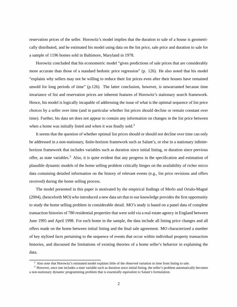
Figure 2.1 illustrates two typical observations in the dataset. We have plotted list prices over the full

duration from initial listing until sale as a ratio of the initial listing price. The red dots plot the first offer

and the blue squares are the second offers received in a match. The stars plot the final accepted transaction

prices. Thus, the seller of property 1046 in the left hand panel of figure 2.1 experienced 3 separate matches.

The first occurred in the fourth week that the property was listed, and the seller rejected the first bid by

a bidder equal to 95% of the list price. The buyer “walked” after the seller rejected the offer. The next

match occurred on the sixth week on he market. The seller onceagain rejected this second prospective

buyer’s first bid, which was only 93% of the list price. However this time the bidder did not walk after

this first rejection, but responded with a second higher offer equal to 95% of the list price. However when

the seller rejected this second higher offer, the second bidder also walked. The third match occurred in the

11th week the home was on the market. The seller accepted thisthird bidder’s opening offer, equal to 98%

of the list price. Note that there were no changes in the initial list price during the 11 weeks this property

was on the market.

The right hand panel plots a case where there was a decrease inthe list price by 5% in the fourth week

this property was on the market. After this price decrease another 5 weeks elapsed before the first offer was

made on this home, equal to 90% of the initial list price. The seller rected this offe and the bidder made a

counteroffer equal to 91% of the initial list price. The seller rejected this second offer too, prompting the

bidder to make a final offer equal to 94.5% of the initial list price which the seller accepted.

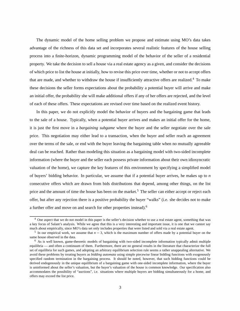
Figure 2.2 plots the number of observations in the data set and the mean and median list prices as a

function of the total number of weeks on the market. The left hand panel plots the number of observations

(unsold homes reamining to be sold) as a function of durationsince initial listing. For example only 54

10

2 4 6 8 10 120.9

0.92

0.94

0.96

0.98

1

Weeks on Market

List

Pric

e an

d O

ffers

List Price and Offer History for House ID 1046 (observation # 46)

1 2 3 4 5 6 7 8 9 100.88

0.9

0.92

0.94

0.96

0.98

1

Weeks on Market

List

Pric

e an

d O

ffers

List Price and Offer History for House ID 1050 (observation # 50)

Figure 2.1 Selected Observations from the London Housing Data

of the 780 observations remain unsold after 30 weeks on the market, so over 93% of the properties listed

by this agency sell within this time frame. If we compute the ratio of first offers received to the number

of remaining unsold properties, we get a crude estimate of the offer arrival rate (a more refined model and

estimate of this rate and its dependence on the list price will be presented subsequently). There is an 11%

arrival rate in the first week a home is listed, meaning that approximately 11% of all properties will receive

one or more offers in the first week after the home is listed with the real estate agency. The arrival rate

increases to approximately 15% in weeks 2 to 6, then it decreases to approximately 12% in weeks 7 to 12,

and then drops to about 10% thereafter, although it is harderto estimate arrival rates for longer durations

given the declining number of remaining unsold properties.

The right hand panel of figure 2.2 plots the mean and median list prices of all unsold homes as a

function of the duration on the market. We have normalized the list prices by dividing by the predicted sale

price from a hedonic price regression using the extensive set of housing characteristics that are available

in the data set (e.g. location of home, square meters of floor space, number of baths, bedrooms, and so

forth). However the results are approximately the same whenwe normalize using theactual transaction

prices instead of the regression predictions: this is a consequence of the fact that the hedonic regression

provides a very accurate prediction of actual transaction prices.

We see from the right panel of figure 2.2 that initially housesare listed at an average of a 5% premium

above their ultimate selling prices, and there is an obviousdownward slope in both the mean and median

11

0 10 20 30 40 50 60 70 800

100

200

300

400

500

600

700

800

Weeks on the Market

Num

bers

of O

bser

vatio

ns o

n Li

st a

nd O

ffer

Pric

es

Numbers of List/Offer Price Observations for London markets with 780 homesNumber receiving offers: 780, min,mean,max duration to sale (weeks): (1,10,70)

List PriceFirst OfferSecond OfferThird Offer

0 5 10 15 20 25 30 35 400.85

0.9

0.95

1

1.05

1.1

Weeks on the Market

Mea

n an

d M

edia

n Li

st P

rice

(as

a ra

tio o

f hed

onic

val

ue)

List Price for Unsold Homes: Mean Number of List Price Changes: 1.2Percent of homes with (0,1,2,2+) changes: (77.3,20.8, 1.9, 0.0)

MeanMedian

Figure 2.2 Number of Observations and List Prices by Week on Market

list prices as a function of duration on the market. However the slope is not very pronounced: even

after 25 weeks on the market the list price has only declined by 5%, so that at this point list prices are

approximately equal to theex anteexpected selling prices. The apparently continuously downward slope

in mean and median list prices is misleading in the sense that, as we noted from figure 2.1, individual list

price trajectories are piecewise flat with discontinuous jumps on the dates where price reductions occur.

Averaging over these piecewise flat list price trajectoriescreates an illusion that list prices are continuously

declining as a function of duration on the market, but we emphasize again that the individual observations

do not have this property.

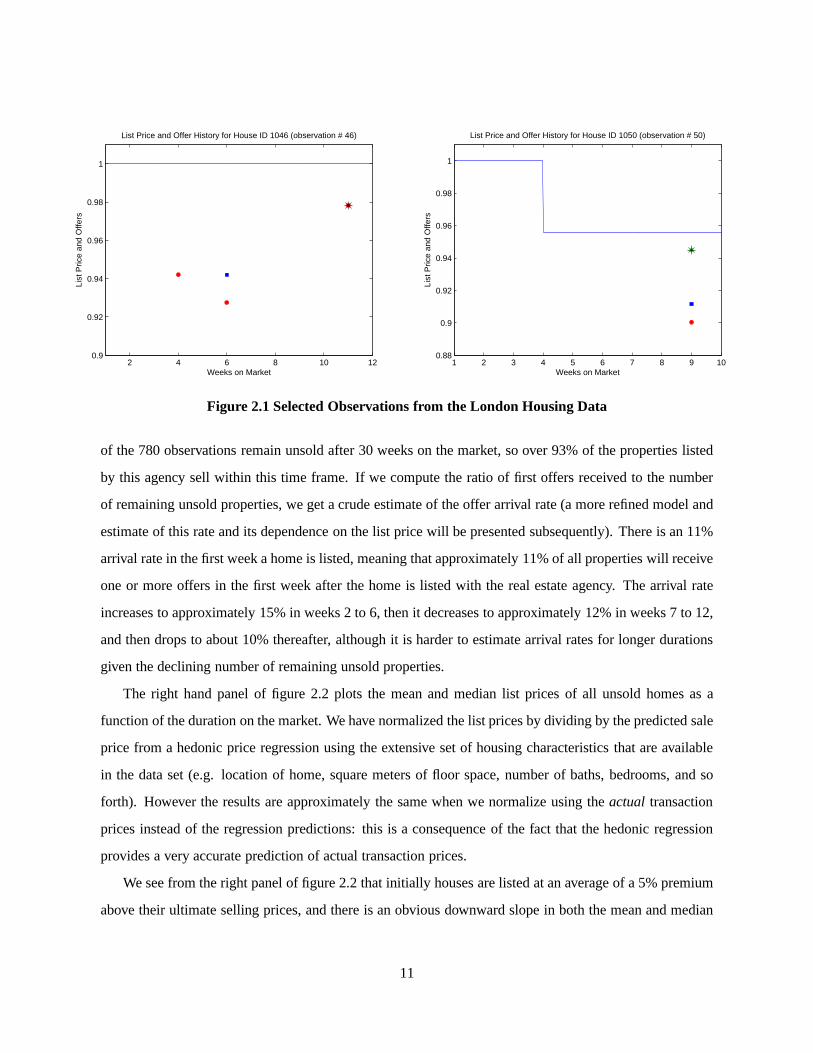
Figure 2.3 plots the distribution of sales prices (once again normalized as a ratio to the predicted trans-

action price) and the distribution of duration to sale. The left hand panel of figure 2.3 plots the distribution

of sales price ratios. There are two different distributions shown: the blue line is the distribution of ratios

of sale price to the hedonic prediction of sales price, and the red line is the distribution of the ratio of sales

price to the initial list price, multiplied by 1.05 (this latter factor is the average markup of the initial list

price over the ultimate transaction price, as noted above).Both of these distributions have a mean value

of 1 (by construction), but clearly the distribution of the adjusted sales price to list price ratio is much

more tightly concentrated than the distribution of sales price to hedonic value ratios. Evidently there is

significant information about the value of the home that affects the seller’s decision of what price to list

their home at that is not contained in thex variables used to construct the hedonic price predictions.The

12

0 0.5 1 1.5 2 2.5 3 3.50

1

2

3

4

5

6

7

8

9

Den

sity

of S

ales

Pric

e

Sales Price Ratio

Distribution of Sales PricesMin, Mean, Median, Max, Std of Sale Price/Hedonic ( 0.22, 1.00, 0.98, 3.38, 0.30)

Min, Mean, Median, Max, Std of Sale Price*1.05/List Price ( 0.53, 1.00, 1.01, 1.32, 0.07)

Sales Price/Hedonic ValueSales Price*1.05/List Price

0 10 20 30 40 50 60 700

0.01

0.02

0.03

0.04

0.05

0.06

0.07

Weeks to Sale

Est

imat

ed D

ensi

ties

Distribution of Duration (in weeks) to SaleMin,Mean,Median and Max ( 1.00,10.27, 6.00,69.00)

Figure 2.3 Distribution of Sale Prices and Duration to Sale

model we present in section 3 will account for this extraprivate informationabout the home that we are

unable to observe. However even when this extra informationis taken into account, there is still a fair

amount of variation/uncertainty in what the ultimate salesprice will be, even factoring in the information

revealed by the initial list price: the sales price can vary from as low of only 53% of the adjusted list price

to 32% higher than the adjusted list price.

The right hand panel of figure 2.3 plots the distribution of times to sale. This is a clearly right skewed

but unimodal distribution with a mean time to sale of 10.27 weeks and a median time to sale of 6 weeks.

As we noted above, over 90% of the properties in our data set were sold within 30 weeks of the date the

property was initially listed. Scatterplots relating timeto sale to the ratio of the list price to the hedonic

value (not shown) do not reveal any clear negative relationship between the degree of “overpricing” (as

indiciated by high values of this ratio) and longer times to sale. Thus, we do not find any clear evidence at

this level supporting the “loss aversion” explanation advocated by Genesove and Mayer (2001). However

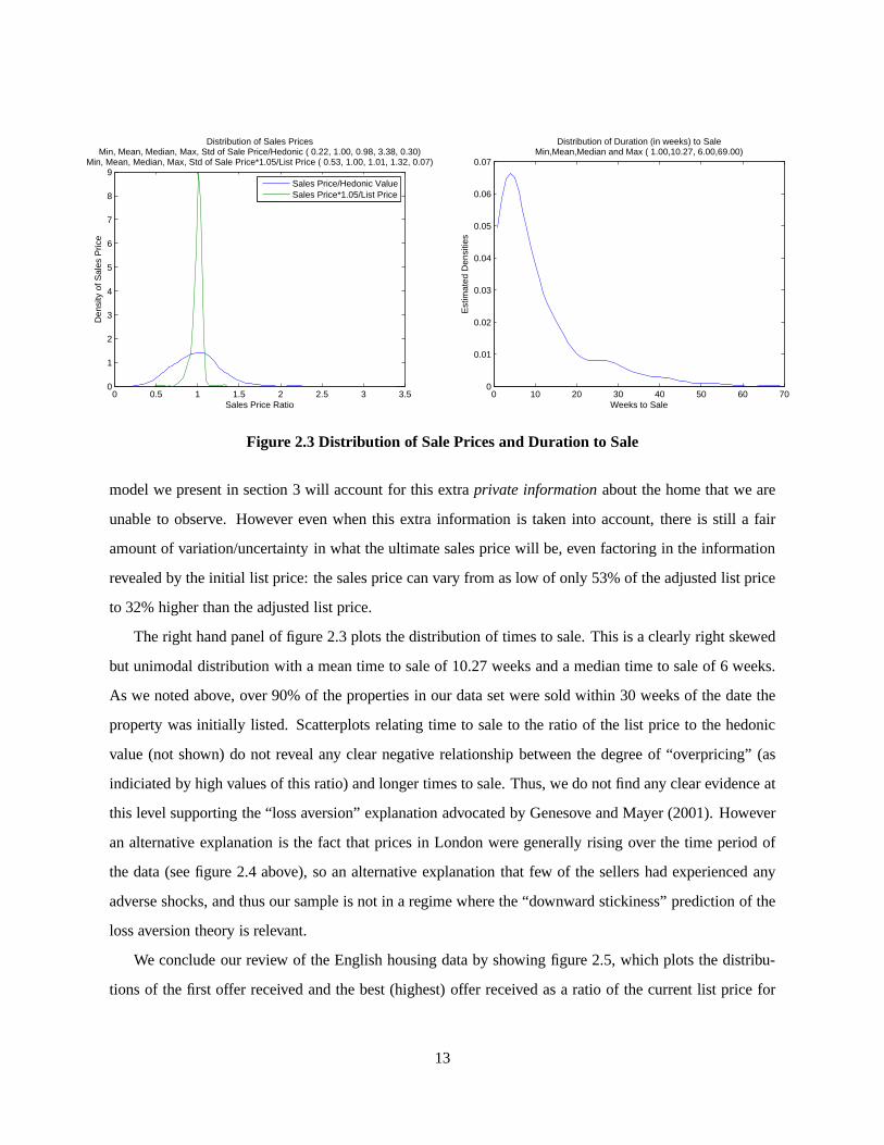
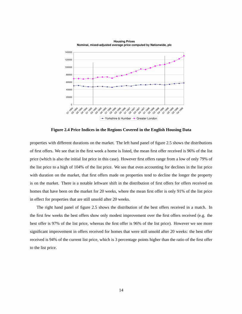
an alternative explanation is the fact that prices in Londonwere generally rising over the time period of

the data (see figure 2.4 above), so an alternative explanation that few of the sellers had experienced any

adverse shocks, and thus our sample is not in a regime where the “downward stickiness” prediction of the

loss aversion theory is relevant.

We conclude our review of the English housing data by showingfigure 2.5, which plots the distribu-

tions of the first offer received and the best (highest) offerreceived as a ratio of the current list price for

13

Housing Prices

Nominal, mixed-adjusted average price computed by Nationwide, plc

0

20000

40000

60000

80000

100000

120000

140000

Q1

1994

Q2

1994

Q3

1994

Q4

1994

Q1

1995

Q2

1995

Q3

1995

Q4

1995

Q1

1996

Q2

1996

Q3

1996

Q4

1996

Q1

1997

Q2

1997

Q3

1997

Q4

1997

Q1

1998

Q2

1998

Q3

1998

Q4

1998

Q1

1999

Q2

1999

Q3

1999

Q4

1999

Yorkshire & Humber Greater London

Figure 2.4 Price Indices in the Regions Covered in the English Housing Data

properties with different durations on the market. The lefthand panel of figure 2.5 shows the distributions

of first offers. We see that in the first week a home is listed, the mean first offer received is 96% of the list

price (which is also the initial list price in this case). However first offers range from a low of only 79% of

the list price to a high of 104% of the list price. We see that even accounting for declines in the list price

with duration on the market, that first offers made on properties tend to decline the longer the property

is on the market. There is a notable leftware shift in the distribution of first offers for offers received on

homes that have been on the market for 20 weeks, where the meanfirst offer is only 91% of the list price

in effect for properties that are still unsold after 20 weeks.

The right hand panel of figure 2.5 shows the distribution of the best offers received in a match. In

the first few weeks the best offers show only modest improvement over the first offers received (e.g. the

best offer is 97% of the list price, whereas the first offer is 96% of the list price). However we see more

significant improvement in offers received for homes that were still unsold after 20 weeks: the best offer

received is 94% of the current list price, which is 3 percentage points higher than the ratio of the first offer

to the list price.

14

0.75 0.8 0.85 0.9 0.95 1 1.05 1.1 1.150

2

4

6

8

10

12

14

First Offer (as a ratio of list price)

Est

imat

ed D

ensi

ties

Distribution of First Offers as a ratio of List PriceMin, Mean, Median and Max of:

Offers week 1 ( 0.79, 0.96, 0.96, 1.04)Offers week 10 ( 0.86, 0.96, 0.96, 1.00)Offers week 20 ( 0.83, 0.91, 0.92, 0.99)

Initial listingAfter 10 weeksAfter 20 weeks

0.8 0.85 0.9 0.95 1 1.050

5

10

15

Best Offer (as a ratio of list price)

Est

imat

ed D

ensi

ties

Distribution of Best Offers as a ratio of List PriceMin, Mean, Median and Max of:

Offers week 1 ( 0.82, 0.97, 0.98, 1.03)Offers week 10 ( 0.86, 0.96, 0.97, 1.00)Offers week 20 ( 0.83, 0.94, 0.95, 1.00)

Initial listingAfter 10 weeksAfter 20 weeks

Figure 2.5 Distribution First Offer and Best Offer as a Ratio of List Price

3 The Seller’s Problem

This section presents our formulation of a discrete-time, finite-horizon dynamic programming problem of

the seller’s optimal strategy for selling a house. The modelwe propose incorporates several features of the

house selling process in England illustrated in the previous section.

Since our data set only includes properties that were listedand sold via a real estate agent, we take

the decision to sell a house (via a real estate agency) as a given, and consider the seller’s decisions of

which price to list the house at initially, how to revise thisprice over time, whether or not to accept offers

that are made, and whether to withdraw the house if insufficiently attractive offers are realized. To make

these decisions the seller forms expectations about the probability a potential buyer will arrive and make

an initial offer, the probability she will make additional offers if any of her offers are rejected, and the level

of each of these offers. These expectations are revised overtime based on the realized event history.

We do not explicitly model the behavior of buyers and the bargaining game that leads to the sale of

a house. Rather, we capture the salient features of the bargaining environment by specifying a simplified

model of buyers’ bidding behavior. In particular, we assumethat if a potential buyer arrives, she makes up

to 3 consecutive offers (where 3 is the maximum number of offers observed in the data), which are drawn

from bids distributions that depend, among other things, onthe list price and the amount of time the house

has been on the market.12 The seller can either accept or reject each offer, but after any rejection there is a

12 We describe this component of our model in detail in the next section.

15

positive probability the buyer “walks” (i.e. she decides not to make a further offer and move on and search

for other properties instead). As explained above, the procedure where a potential buyer makes offers that

the seller can simply either accept or reject mimics the negotiating protocol in the data.

A decision period is a week, and we assume a finite horizon of 2 years. If a house is not sold after 2

years, we assume that it is withdrawn from sale and the sellerobtains an exogenously specified “continua-

tion value” representing the use value of owning (or renting) their home over a longer horizon beyond the

2 year decision horizon in this model.13

The seller’s continuation value will generally be different from a quantity we refer to as the seller’s

financial valueof their home. This is the seller’s expectation of what the ultimate selling price will be for

their home. While it is clear that the ultimate selling priceis endogenously determined and partly under

control of the seller, we can think of the financial value as a realistic appraisal or initial assessment on

the part of the seller of the ultimate outcome of the selling process. Since the seller’s optimal strategy

will depend on the financial value of the house, if the financial value is to represent a rational, internally

consistent belief on the part of the seller, it will have to satisfy a fixed-point condition that guarantees that

it is a “self-fulfilling prophecy”. Although we do not explicitly enforce this fixed-point constraint in our

solution of the dynamic programming problem, we verify below (via stochastic simulations) that it does

hold for the estimated version of our model.14

Let F0 denote the seller’s perception about the financial value of their home at the time of listing. We

assume thatF0 is given by the equation

F0 = exp{Xβ+ η0} (1)

whereX are the observed characteristics of the home (the basis for the traditional hedonic regression

prediction of the ultimate sales price discussed in Section2), andη0 reflects the impact of other variables

that are observed by the seller but not by the econometricians that can affect the seller’s perception of their

13 The continuation value may include the option value of relisting the home at a future date, perhaps during a period whereconditions in the housing market are more favorable to the seller. However, we do not model the decision that leads eitherto“entry” (i.e. the initial decision to sell) or to “re-entry”(in case the property is withdrawn and then re-listed) of a house on themarket.

14 While it is possible to enforce the rationality constraint as a fixed-point condition on our model, from our standpoint itisuseful to allow for formulations that relax the rationalityconstraint. This gives us the additional flexibility to consider modelswhere sellers do not have fully rational, self-consistent beliefs about the financial value of their homes. Indeed, allowing forinconsistent or “unrealistic” beliefs may be an alternative way to explain why some home sellers set unrealistically high listingprices for their homes that would be distinct from the loss aversion approach discussed in the introduction. However, aswe showbelow, we do not need to appeal to any type of irrationality orassume that sellers have unrealistic beliefs in order to provide anaccurate explanation of the English housing data.

16

home’s financial value. These variables could include the seller’s private assessment of aggregate shocks

that affect the entire housing market, regional or neighborhood level shocks, as well as idiosyncratic house-

specific factors. We assume that after consultation with appraisers and the real estate agent, the seller has

a firm assessment of the financial value of their home that doesnot vary over the course of their selling

horizon. Hence,η0 can be interpreted as reflecting the seller’sprivate informationabout the financial value

of their home that is not already captured by the observable characteristicsX.

Recall the left panel of figure 2.3 that shows that the adjusted list price is a far more accurate predictor

of the ultimate selling price of the home than the hedonic value, exp{Xβ}. In our estimation of the

model, we assume that exp{η0} is a lognormally distributed random variable that is independent ofX, and

we estimateβ via a log-linear regression of the final transaction price onthe X characteristics assuming

that the random variable exp{ν0} satisfies the restrictionE{exp(η0)} = 1. This restriction represents the

rationality constraintwe refer to above, which we verify is satisfied by our estimated model.

Due to the fact that the seller’s optimal selling decisions depend critically on the seller’s financial

valueF0, which in turn depends on a very high dimensional vector of observed housing characteristics

X as well as unobserved componentsη0, straightforward attempts to solve the seller’s problem while

accounting for all of these variables immediately presentsus with a significant “curse of dimensionality”.

In principle, we could treat the estimated hedonic value exp{Xi β} as a “fixed effect” relevant to propertyi

and solveN = 780 individual dynamic programming (DP) problems, one for each of the 780 properties in

our sample. However, the problem is more complicated due to the existence of the unobserved “random

effect” η0. This is a one dimensional unobserved random variable and inprinciple we would need to solve

each of the 780 DP problems over a grid of possible values ofη0, and thereby approximate the optimal

selling strategy explicitly as a function of all possible values of the unobserved random effectη0, which

would be then “integrated out” in the estimation of the model.

However, by imposing alinear homogeneityassumption, we can solve a single DP problem for the

seller’s optimal selling strategy where the values and states are defined asratios relative to the seller’s

financial value.In particular, define the seller’s current list pricePt to be the ratio of the actual list price

divided by the seller’s financial valueF0. ThenPt = 1.0 is equivalent to a list price that equals the financial

value, andPt > 1.0 corresponds to a list price that exceeds the financial valueand so forth. The implicit

assumption underlying the linear homogeneity assumption is that, at least within the limited and fairly

homogeneous segment of the housing market in our data set, there are no relevant further “price subseg-

17

ments” that have significantly different arrival rates and buyer behavior depending on whether the houses

in these segments are more expensive “high end” homes or not.The homogeneity assumption reflects a

reasonable assumption that arrival rates and buyer biddingbehavior are driven mostly by whether a given

home is perceived to be a “good deal” as reflected by the ratio of the list price to the financial value. How-

ever, as we discuss below, the actual bid submitted by a buyerwill depend on the buyer’s private valuation

for the home (also expressed as a ratio of the financial valueF0).

Let St(Pt ,dt) denote the expected discounted (optimal) value of selling the home at the start of week

t, where the current ratio of the list price to the financial value isPt , and where the duration since the

last match isdt , with dt = 0 indicating a situation where no matches have occurred yet.Here a match is

defined as a buyer who makes an offer on the home. We will get into detail about the timing of decisions

and the flow of information shortly, but already we can see that this formulation of the seller’s problem

has three state variables: 1) the current total time on the market t, 2) the duration since the last match

dt , and 3) the current list price to financial value ratioPt . The value functionSt(Pt ,dt) provides the value

of the home as a ratio of the financial value, so to obtain the actual value and actual list price we simply

multiply these values byF0. ThusF0St(Pt ,dt) is the present discounted value of the optimal selling strategy,

andF0Pt is the current list price, both measured in UK pounds (£). Via this “trick” we can account for

substantial heterogeneity in actual list prices and sellervaluations by solving just a single DP problem “in

ratio form.” However an important implication of this assumption is that timing of list price reductions and

the percentage size of these reductions implied by the seller’s optimal selling strategy are homogeneous of

degree 0 in the list price and the financial value.

Our model of the optimal selling decision does not require the seller to sell their home within the 2

year horizon: we assume that the seller has the option to withdraw their home from the market at any time

over the selling horizon. Since we do not model the default option of not selling one’s house, we do not

attempt to go into any detail and derive the form of the value to the seller of withdrawing their home from

the market and pursuing their next best option (e.g. continuing to live in the house, or renting the home).

Instead we simply invoke a flexible specification of the “continuation value”Wt(Pt ,τ) of withdrawing a

home from the market and pursuing the next best opportunity.15

15 Alternatively, we could allow for different types of sellers who have different continuation values and specifyWt (Pt ,τ),where the parameterτ could denote the seller’s “type.” Fortunately, however, although our model can allow for other types ofunobserved heterogeneity beyond the privately observed component of the financial valueη0, we did not need to appeal to anytype of unobserved heterogeneity in seller types in order for the model to provide a good approximation to the behavior we

18

The seller has 3 main decisions: 1) whether or not to withdrawthe property, 2) if the seller opts not

to withdraw the property, there is a decision about which list price to set at the beginning of each week

the home is on the market, and 3) if a prospective buyer arrives within the week and makes an offer, the

seller must determine whether or not to accept the offer, andif the seller rejects the offer and the buyer

makes a second offer, whether to accept the second offer, andso on up to (possibly) a third and final offer.

We assume that the first two decisions are made at the start of each week and that the seller is unable to

withdraw their home or change their list price during the remainder of the week. Within the week, if one

or more offers arrive, the seller decides whether or not to accept them.

The Bellman equation for the seller’s problem is given in equation (??) below.

St(Pt ,dt) = max

[

Wt(Pt),maxP

[ut(P,Pt ,dt)+ βESt+1(P,Pt ,dt)]

]

(2)

The Bellman equation says that at each weekt, the optimal selling strategy involves choosing the larger

of 1) the continuation value of (permanently) withdrawing the home from the market, or 2) continuing to

sell, choosing an optimal listing priceP. The functionESt+1(P,Pt ,dt) is the conditional expectation of the

weekt +1 value functionSt+1 conditional on the current state variables(Pt ,dt) and the newly chosen list

priceP. Pursuant to the “forward-looking” perspective that we discussed in the introduction, in the version

of the model we actually estimate in the next section, this expectation depends only onP and not on the

previous week’s list pricePt . That is, the current list priceP is a sufficient statistic affecting the arrival

rate of buyers and the magnitude of bids submitted. However one could imagine a world with information

lags where arrival rates and bids could depend on previous list prices, including the last week list price

Pt . While it is not hard to allow for such lags without greatly complicating the solution of the model (at

least provided we only allow a single week lag), we have foundthat it was not necessary to account for

information lags to enable the model to provide a good approximation to the behavior we observe in the

English housing data.

The functionut(P,Pt ,dt) captures two things: 1) the fixed “menu cost” of changing the list price, and

2) the “holding cost” to the seller of having their home on themarket.

ut(P,Pt ,dt) =

−ht(dt)−K if P 6= Pt

−ht(dt) if P = Pt

(3)

observe in the English housing data.

19

The functionht(dt) is the net disutility (in money equivalent units) of having to keep the house in a tidy

condition and to be ready to vacate it on short notice so the real estate agent can show it to prospective

buyers.K is the fixed menu cost associated with changing the list price. This fixed cost can include the

cost of posting new advertisements in a newspaper and/or websites, and printing up new flyers with the

new listing price, and other bureaucratic costs involving in making this change (i.e. consulting with the

realtor to determine the best new price to charge). We would expect thatK should be a small number since

none of the costs listed above would be expected to be large inabsolute terms.

We now write a formula forESt+1(P,Pt ,dt) that represents the value of the within week events when

a match occurs. To keep the notation simpler, we will omitPt from this conditional expectation, since as

we noted above, we did not need to includePt to capture any information lags that might affect arrival

of buyers or the bids they might make. In order to describe theequation forESt+1, we need to introduce

some additional information to describe the seller’s beliefs about the arrival of offers from buyers, the

distribution of the size of the offers, and the probability that the buyer will walk away (i.e. not make a

new offer and search for other houses) if the seller rejects the buyer’s offer. Given the negotiation protocol

described above, within a given week there are at most 3 possible stages of offers by a potential buyer and

accept/reject decisions by the seller. To simplify notation, we writeESt+1 for the case where at most one

buyer arrives and makes an offer on the home in any week.16

Let λt(P,dt) denote the conditional probability that an offer will arrive within a week given that the

seller set the list price to beP at the start of the week and the duration since the last offer is dt . Let O j

be the highest offer received at stagej = 1,2,3 of the “bargaining process.” Letf j(O j |O j−1,P,dt) denote

the seller’s beliefs about the offer the buyer would make at stage j given that the buyer did not walk in

response to the seller’s rejection of the buyer’s offer in stage j −1. If the seller accepts offerO j , let Nt(O j)

denote the net sales proceeds (net of real estate commissions, taxes, and other transactions costs) received

by the seller. The seller must decide whether to accept the net proceedsNt(O j), thereby selling the home

and terminating the selling process, or reject the offer andhope that the buyer will submit a more attractive

offer, or that some better offer will arrive from another potential buyer in some future week.

If a seller rejects the offerO j , there is a probabilityω j(O j ,P,dt) that the buyer will “walk” and not

make a new offer as a function of the last rejected offer,O j , and the current state(P,dt). With this notation

16 Note however that our framework also accommodates the possibility of “auctions”, i.e. situations where multiple buyers arebidding simultaneously for a home.

20

we are ready to write the equation for the within week problemwhich determinesESt+1 and completes

the Bellman equation. We have

ESt+1(P,dt) = λt(P,dt)St+1(P,dt)+ [1−λt(P,dt)]

∫

O1

max[

Nt(O1),ES1t+1(O1,P,dt)

]

f1(O1|P,dt)dO1.

(4)

The functionES1t+1(O1,P,dt) is the expectation of the subsequent stages of the within-week “bargaining

process” conditional on having received an initial offer ofO1 and conditional on the beginning of the week

state variables,(P,dt). We can write a recursion for these within-week expected value functions similar to

the overall backward induction equation for Bellman’s equation as a “within-period Bellman equations”

ES1t+1(O1,P,dt) = ω1(O1|P,dt)St+1(P,dt +1)+

[1−ω1(O1|P,dt)]∫

O2

max[

Nt(O2),ES2t+1(O2,P,dt)

]

f2(O2|O1,P,dt)dO2. (5)

and

ES2t+1(O2,P,dt) = ω2(O2|P,dt)St+1(P,dt +1)+

[1−ω2(O2|P,dt)]

∫

O3

max[Nt(O3),St+1(P,1)] f3(O3|O2,P,dt)dO3. (6)

What equation (??) tells us is that after receiving 2 offers and rejecting the second offerO2, the seller

expects that with probabilityω2(O2|P,dt) the buyer will walk, so that the bargaining ends and the seller’s

expected value is simply the expectation of next periods’ value St+1(P,dt +1). However, with probability

1−ω2(O2|P,dt), the buyer will submit a third and final offerO3 which is a draw from the conditional

density f (O3|O2,P,dt). Once the seller observesO3, he can either take the offer and receive the net

proceedsNt(O3), or reject the offer, in which case the potential buyer leaves for sure and the seller’s

expected value is the next week value function,St+1(P,1). Note that the second argument, the duration

since last offer, becomes 1 at weekt +1 reflecting that an offer arrived at weekt.

4 Models of Bidding by Prospective Buyers

Our initial intention was to develop a highly flexible model of buyer behavior that could be consistent with

a wide range of theories of buyer behavior. We attempted to estimate the distribution of the first offer

f1(O1|P,d) and the conditional densitiesf j(O j |O j−1,P,d) representing the improvement in bids when the

21

seller rejects the previous bid and the buyer offers at bidding stages 2 and 3 using non-parametric and semi-

parametric estimation methods in a semi-parametric two-step approach to the estimation of our model of

seller behavior.

Unfortunately, this strategy did not work. Although we wereable to estimate the bid densitiesf j under

fairly weak assumptions, when we used these estimated densities to solve for the optimal selling problem

we obtained unreasonable results, including predictions that the seller should set infinite list prices.

One important fact about observed bidding behavior is thatthere is a positive probability that a

prospective buyer will submit a bid equal to the current listprice. In the English housing data, over

15 percent of all accepted offers are equal to the list price and over 10 percent of allfirst offers are equal

to the list price. Further, we also observe offers inexcessof the seller’s list price. For example, over 2%

of all first offers are above the list price, and nearly 4% of all accepted offers are higher than the list price

prevailing when the offer was made.

Thus, any estimation of the offer distributions needs to account for mass points in the distribution,

particularly at the list price. We found that we obtained unreasonable implications for the seller model

even when we imposed a fair amount of parametric assumptionson the offer distributions, which were

intended to help enforce “reasonable” behavioral implications for the seller.

One of these parametric models is a double beta distributionwith a mass point at the list price. An

example of the double beta density function for bids is presented in the left hand panel of figure 4.1 below.

There is a right-skewed component of the bid distribution tothe left of the list price mass point, and then

a smaller left skewed beta distribution above this mass point. The most important part is the piece below

the list price, which captures the “underbidding” that is the predominant outcome of matches between a

buyer and the seller. The right skewed beta component has as its support the interval[.25,1] where we

have normalized the bid as a ratio of the current list price ofthe house,P. Thus, the lower support.25

represents a bid equal to 1/4 of the current list price of the home.

The distribution plotted in the left hand panel of figure 4.1 is actually a rescaled version of the double

beta distribution. The figure does not include the mass pointat the list price due to problems with plotting

density values and the mass point on the same scale. The beta density component to the left of the mass

point the list price has been scaled to have a total mass of.85, representing the probability that a bid will

be strictly below the list price. The component of the beta distribution above 1 is scaled to have a total

mass of.05, representing a 5% probability of receiving a bid strictly above the list price. The remaining

22

0.2 0.4 0.6 0.8 1 1.2 1.4 1.60

0.5

1

1.5

2

2.5

3

3.5

4

4.5

5

Bid (as a fraction of list price)

Den

sity

Example of Double Beta Density for Bids

0 0.5 1 1.5 2 2.5 3 3.5 40

0.5

1

1.5

2

2.5

3

3.5

4Expected Bid as a function of R, week= 4, bidding stage=1

List price ratio, R

Exp

ecte

d B

id (

as a

rat

io o

f hed

onic

val

ue)

Figure 4.1 Double Beta Distribution of Bids and the implied expected bid function

mass is a 10% probability of receiving a bid equal to the list price.

Based on initial empirical work, we judged this double beta model to be a good approximation to

the actual distribution of bids we observe in the English housing data. The double beta distribution was

specified so that the probabilities of receiving a bid below,equal to, or strictly above the list price was

given by a trinomial logit model and the(a,b) parameters of the beta distributions were specified as

(exponential) functions of state variables in the model (e.g. number of weeks on the market, the list price,

and other variables). Unfortunately, as we see in the right hand panel of figure 4.1, the results of this

model have unreasonable implications for sellers’ beliefsabout the relationship between the list price and

the expected bid submitted by buyers. The expected bid function is a monotonically increasing function

of the list price. It seems quite unreasonable that a seller should expect to receive to roughly double the

expected bid on his house by doubling the list price, but thisis exactly what the results from an unrestricted

reduced form estimation of the offer distribution implies!

Further, our reduced form estimation results for the arrival rate of matches resulted in apositiverela-

tionship between list price and arrival rates of buyers, even after controlling for unobserved random effects,

as represented by theν0 term in the seller’s financial value of the home. Combining these two results, it

is clear that any seller with such beliefs would find it optimal to set an arbitrarily large list price for their

homes, something we never observe in practice. So clearly there is some problem with the flexible two

step approach to estimating the seller model.

23

The problems we experienced are probably not due to a misspecification of beliefs, since our reduced

form model is a highly flexible specification capable of closely approximating the actual distribution of

bids (and rates of arrival of matches). We believe the problem is due to theendogeneity of list prices.In

particular, unobservable characteristicsη0 that increase the financial value of a home also tend to increase

the list price, and also bids made on a home. If we fail to control for these unobservables (as we have

in our initial reduced form estimations), it is perfectly conceivable that the endogeneity problems could

be strong enough to produce the spurious and implausible monotonic relationship between list price and

expected bid values that we see in figure 4.1.

It might be possible to try to use more sophisticated reduced-from econometric methods to overcome

the endogeneity problems. However it is clear that the seller’s behavior is largely determined by the seller’s

beliefs about buyers. Particularly important are the seller’s beliefs about how the list price affects the rate

of arrival of offers and distribution from which these offers are drawn from when they do arrive. Thus,

there is a huge amount of information that can be brought to bear in estimating these rather slippery objects

by adopting a fully structural, simultaneous approach to estimation where we estimate the sellers beliefs

along with the other unknown parameters of the seller (e.g. the discount rate, and the parameters affecting

hassle costs, and so forth) using a nested numerical solution approach. Under this approach we would

solve the seller’s dynamic programming problem repeatedlyfor different trial values of the parameters

governing the seller’s beliefs as well as the other parameters of the model. Trial parameter values that

produce “unreasonable” beliefs for the seller (such as shown in figure 4.1) would be discarded by this

algorithm since these parameter values imply an optimal selling strategy that is greatly at odds with the

behavior we observe in the data.

While it may ultimately be possible to estimate fairly flexible specifications for sellers’ beliefs about

buyer bids and arrival rates (such as the double beta distribution and even more flexible semiparametric

specifications for the offer distributions), we have decided that it would be best to start by providing more

structure on the bid distribution. There are two main reasons for this. First, even if we were able to

successfully estimate the parameters of the double beta model as structural parameters in a maximum

likelihood or simulated minimum distance estimator, therewould be the issue of how to interpret these

estimated coefficients in terms of an underlying model of bidder behavior.

Instead, we felt that more insight could be gained by trying to build some sort of rudimentary model

of bidding behavior on the part of buyers. By placing more structure on the offer distributions we obtained

24

much more control over the estimation of the model. This is especially important since small movements

in the parameters for beliefs can result in “unreasonable beliefs” and these unreasonable beliefs can lead

to discontinuous “bang-bang” type shifts in the optimal selling strategy. The semi-reduced form model

has fewer free parameters than the more flexibly specified reduced form models of bidding behavior, the

parameters are more readily interpretable, and it is easierto see whether the estimated parameters are

unreasonable or not, and how to constrain parameters to “reasonable” sections of the parameter space.

The “semi-reduced form model” of buyers’ bidding behavior derives the distribution of bids from

two underlying “semi-structural” objects: 1) a specification of buyers’ bid functions,b(v, l ,F), and 2) a

specification of the distribution of buyer valuations,h(v|F, l), wherev is the buyer’s private valuation of

the home,F is the financial value of the home, andl is the current list price. In order to maintain the

homogeneity restriction, we assume thatl andF only enterb andh in a ratio form, i.e. asp = l/F . Thus,

in the subsequent notation we will write these objects asb(v, p) andh(v|p).

We put “structural” in quotes because a fully structural model of buyer behavior would derive the

buyers’ bid functions from yet deeper structure: from the solution to their search and bargaining problem.

We eventually want to extend the model in this direction, butsince the English housing data contain

relatively little data on buyers other than the bids they make in matches observed in the data set, it seems

sensible to start out with a less complicated and detailed model of their behavior. In particular, since we

do not have any data that follows buyers as they search among different homes and allow us to see homes

they visit and don’t make offers on and homes they visit and domake offers on, it seems that a more

complicated buyer search model will have many additional parameters characterizing buyer search costs

and opportunity sets and preferences for different locations and types of houses. The presence of so many

additional parameters in the absence of good data on how buyers actually search and decide which houses

to bid on could lead to severe identification problems if we have to rely only on a highly self-selected data

set of actual matches. This is our justification for failing to pursue a more detailed model of buyer behavior

at this point.

The simplest specification for bid functions that we could think of that yields an offer distribution with

a mass point at the current list price of the house is the following class of piecewise linear bid functions:

b(v, p) =

r1(p)v if v∈ [v,v1)

p if v∈ [v1,v1 +k(p))

r2(p)v if v∈ [v1 +k(p),v]

(7)

25

wherev andv are the lower and upper bounds, respectively, on the supportof the distribution of buyer

valuations (to be discussed shortly). To ensure continuityof b(v, l) as a function ofv, r1 andr2 must satisfy

the following restrictions

p = r1(p)v1

p = r2(p)(v1 +k(p)) (8)

This implies that

v1 =p

r1(p)

r2(p) =p

l/r1(p)+k(p)(9)

Thus, the bid functions are fully determined by the two functions r1(p) and k(p). The first function

determines how aggressive the bidder will be in terms of whatfraction of the buyer’s true valuation the

buyer is willing to bid, for the first bid (we will consider specifications for 2nd and 3rd bid functions

below). The closerr1(p) is to 1 the more “aggressive” the buyer is in his/her bidding (i.e. the closer they

are to truthful bidding). We assume that the buyer interprets the list pricel as a signal from the seller about

what the seller’s reservation value is and as a signal of how reasonable the seller is. If the list price ratio

p is substantially bigger than 1, the buyer will interpret this as a sign of an “unreasonable” list price by

the seller, and so the buyer will respond by shading their bidto a higher degree. Conversely, a seller that

“underprices” their home by setting a list price less than the financial value will result in more aggressive

bidding by buyers, i.e.r1(p) will be closer to 1 whenp < 1. Thus, we posit thatr ′1(p) < 0, so that a seller

who considers overpricing their home will expect that buyers will shade their first bids to a greater degree.

The bid functions have a flat segment equal to the list price for valuations in the interval[v1,v1+k(p)].

As we noted above, this flat section is empirically motivatedby the fact that we observe a mass point in

bid distributions at the list price. By adjusting the lengthof this flat segmentk(p) we can affect the size of

the mass point in the bid distribution and thereby attempt tomatch observed bid distributions.

We posit thatk′(p) < 0 for reasons similar to the assumption thatr ′1(p) ≤ 0: a seller who overprices

his/her home by setting a list price bigger than 1 will resultin a shorter range of valuations over which

buyers would be willing to submit a first offer equal to the list price. Conversely, if a seller underprices

his/her home by setting a list price less than 1, there shouldbe a wider interval of valuations over which

the buyer is willing to submit a first offer equal to the list price. Observe that since the probability of a first

26

offer equal to the list price is the probability that valuations fall into the interval[v1,v1 + k(p)], it is not

strictly necessary fork′(p) ≤ 0 in order for the probability of making an offer equal to the list price to be a

declining function ofl , which is another feature we observe in the English housing data. However initially

we will assume thatk′(p) ≤ 0, but we can obviously consider relaxations of this condition later.

The left hand panel of Figure 4.2 plots examples of bid functions for four different values ofp. These

bid functions were generated from the following specifications for the functionr1(p) andk(p):

r1(p) = .98(1− γ(p))+ .85γ(p)

k(p) = .12(1− γ(p))+ .07γ(p) (10)

where

γ(p) =p−vv−v

. (11)

We see that the bid function for the highest list price, i.e. for a list price ofp = 1.62 given by the blue

dotted line in the left hand panel of figure 4.2, involves the most shading and lies uniformly below the bid

functions at other list prices. It follows that the list price of p = 1.62 isdominatedin terms of revenue to

the seller by lower list prices. However, at more moderate list prices, the bid functions generally cross each

other and so there is no unambiguous ranking based on strict dominance of the bid functions. For example

if we compare the bid function for a list price ofp = 1 with the bid function with a list price ofp = 1.09

(the former is the orange dotted line and the latter is the solid red line in the left hand panel of figure 4.2),

we see that the bid function for the lower list pricep = 1 is higher for buyers with lower valuations and

also for buyers with sufficiently high valuations, but the bid function withp= 1.09 (corresponding to a 9%

markup over the financial value of the home), is higher for an intermediate range of buyer valuations. Thus

the question of which of the two list prices result in higher expected revenues depends on the distribution

of buyer valuations: if this distribution has sufficient mass in the intermediate range of buyer valuations

where the bid function for the higher list pricep = 1.09 exceeds the bid function for the lower list price

p = 1, then the expected bid from setting the higher list price will exceed the expected bid from setting a

lower list price. Of course this statement isconditionalon a buyer arriving and making a bid: we need to

factor in the impact of list price on the arrival rate to compute the overall expected revenue corresponding

to different list prices.

The right hand panel of figure 4.2 shows how the bid functions change in successive bidding stages.

Bid functions for later bidding stages dominate the bid functions for earlier bidding stages, resulting in a

27

0.8 1 1.2 1.4 1.6 1.8

0.8

1

1.2

1.4

1.6

1.8

2Bid functions b(v,l,s), v=valuation, l=list price, s=stage, s=3

Buyer’s valuation (as a ratio of hedonic value)

Buy

er’s

bid

(as

a r

atio

of h

edon

ic v

alue

)

45 degree lineb(v,l=1.09,s=3)b(v,l=1.00,s=3)b(v,l=1.33,s=3)b(v,l=1.62,s=3)

0.8 1 1.2 1.4 1.6 1.8

0.8

1

1.2

1.4

1.6

1.8

2Bid functions at successive biddings stages: b(v,l,s), v=value, l=list price, s=stage

Buyer’s valuation (as a ratio of hedonic value)

Buy

er’s

bid

(as

a r

atio

of h

edon

ic v

alue

)

45 degree lineb(v,l=1.00,s=1)b(v,l=1.33,s=2)b(v,l=1.00,s=3)

Figure 4.2 Piecewise linear bid functions for different list prices and bidding stages

monotonically increasing sequence of bids that is consistent with what we almost always observe in the

English housing data. However, there are intervals of valuations where the bids lie on the flat segment of

the bidding function, so this model can generate a sequence of bids where a previous bid (equal to the list

price) is simply resubmitted by the bidder. This is also something we observe in the English housing data.

We complete the description of the semi-reduced form model by describing assumptions about the

distribution of buyers’ valuations for the home,h(v|p). We assume thath(v|p) is in the Beta family of

distributions and thus it is fully specified by two parameters (a,b), as well as its support,[v,v]. We do

not place any restriction on the distribution of valuations. In particular, it might be the case that buyers

who have relatively higher than average valuations for a given home may choose to make offers: this

would argue for a “positively biased” specification whereE{v|p}> p. The direction of the bias might also

depend on the list price: overpriced homes that have been on the market for a long time might be more

likely to attract “vultures” i.e. buyers with lower than average valuations who are hoping to get a good

deal if the seller “caves”. We could imagine many other typesof stories or scenarios. All of these suggest

allowing for a more general model of valuations of the formft(v|p,d) where the distribution of valuations

of buyers who make an offer on a home with a price ratio ofp also depends on the duration since the last

offer d and the length of time that house has been listed,t.

While there is a value (in terms of additional flexibility in the types of bid distributions that can be

generated) by allowing for flexibility in the distribution of buyer valuations, it is clear that if we allow

28

arbitrary amounts of flexibility then we might run into the same sorts of paradoxes that we illustrated for

the fully reduced form specification of buyer bidding behavior. In particular if the distribution of buyer

valuations shifts upward sufficiently quickly as the list price rises, then it is clearly possible that such a

model could result in expected bids that are a monotonicallyincreasing function ofp, just as we observed

in the double beta specification in figure 4.1. In addition there can be difficult identification problems

since higher bids can be increased by either a) fixing a set of piecewise linear bid functions but shifting

the distribution of valuation to the right, or b) fixing a distribution of valuations but allowing the piecewise

bid functions to rise. For this reason, we have started by fixing the support and(a,b) parameters of the

distribution of valuations and focus on estimating the parameters of the piecewise linear bid functions.

Let B(u|a,b) be a beta distribution on the[0,1] interval with parameters(a,b). We can derive the

distribution of bids from this distribution by first rescaling this distribution to the[v,v] interval to get the

distribution of valuationsH(v) given by

H(v) = Pr{v≤ v} = B((v−v)/(v−v)|a,b) . (12)

The left hand panel of figure 4.3 plots an example of a beta distribution of valuations on the interval

[v,v] = [.5,3] for different values of the(a,b) parameters. These parameters give us the flexiblity to affect

both the mode and the tail behavior of the distributions independently of each other. For fixeda, increases

in b decrease the expected valueE{v} and move the mode towards zeroandthin out the upper tail, whereas

for fixedb, increases ina increase the mode, the mean, and thickens the upper tail ofH(v) although larger

changes are required ina to produce comparably dramatic shifts inH(v) compared with changes inb, at

least fora > 1.

The right hand panel of Figure 4.3 plots the implied probability that an offer equals the list price, as

a function ofp at successive stages of the within week bargaining process for buyers whose distribution

of valuations is a beta distribution on the support[.85,1.8] with parameters(a,b) = (4.5,12). We see that

these implied probabilities are roughly in line with the data for the limited range of list prices that we

observe in the English housing data (i.e. a mean first offer that is roughly equal to the financial value, i.e.

E{b(v, p)} ' 1, where the mean value ofp is approximately equal to 1.05. This implies thatr1(p) ' .95

whenp' .95. Actually, for the specification ofr1(p) given above, we haver1(1.05) = .9248.

The implied distribution of bids,G(x|a,b, p), is given by

G(x|a,b, l) = Pr{b(v, p) ≤ x}

29

0.8 1 1.2 1.4 1.6 1.80

0.5

1

1.5

2

2.5

3

3.5

4Beta Distribution of Buyer Valuations on [0.85,1.8], a=4.5, b=12, mean=1.10909

Buyer’s valuation (as a ratio of hedonic value)

Pro

babi

lity

dens

ity v

alue

0.8 1 1.2 1.4 1.6 1.80

0.05

0.1

0.15

0.2

0.25

0.3

0.35

0.4

0.45

0.5Probability offer equals list price

List price (ratio of hedonic value)

Pro

babi

lity

first

offe

r eq

uals

list

Stage 1Stage 2Stage 3

Figure 4.3 Beta distribution of buyer valuations and implied probabilities of bidding the list price

= Pr{

v≤ b−1(x, p)}

= B(

b−1(x, p)−v)/(v−v)|a,b)

. (13)

Due to the presence of the flat segment, the usual notion of an inverse of the bid functon does not exist.

However if we interpret the inverse of the bid function at thevalue p as the interval[v1,v1 + k(p)], we

obtain a distribution of bids that has a mass point in the distribution of bids at the list price, consistent with

what we observe in the English housing data.

In summary we can write the distribution of bids implied by our semi-reduced form specification of

bidding behavior explicitly in terms of the functionsr1(p) andk(p) as

G(x|a,b, p)=

B((x/r1(p)−v)/(v−v)|,a,b) if x∈ [v, p)

B((k(p)+ p/r1(p)+k(p)−v)/(v−v)|a,b)−B((p/r1(p)−v)/(v−v)|a,b) if x = p

B((x(p/r1(p)+k(p))−v)/(v−v)|a,b) if x∈ (p,v](14)

Using this distribution function, we can compute theexpected bid function E{b|p} as

E{b|p} =∫

xG(dx|a,b, p)

=

∫ v

vb(v, p)H(dv). (15)

Note that the expectation depends both on the list price and on the financial value because bids are inter-

preted as ratios of list price to the financial value of the home.

30

0.8 1 1.2 1.4 1.6 1.80.65

0.7

0.75

0.8

0.85

0.9

0.95

1Expected bid (stages 1, 2, 3) as a function of list price

List price (ratio of hedonic value)

Exp

ecte

d bi

d (r

atio

of h

edon

ic v

alue

)

Stage 1Stage 2Stage 3

Figure 4.4 Expected bids as a function of the list price and bidding stage

Figure 4.4 plots the expected bid functions for several different specifications of the distribution of

valuations. We see that the expected bid functions are unimodal and are maximized at list prices that are

higher than 1, providing an incentive for the seller to “overprice” when the seller sets a list price. Of course

this is not the full story, since the seller must also accountfor the effect of the list price on arrival rates

of buyers. The dynamic programming problem takes both factors into account, as well as other dynamic

considerations and the fixed menu costs involved in changingthe list price.

5 Empirical Results

This section presents econometric estimates of our model ofthe house seller’s decision via two different

estimation methods: a (quasi) maximum likelihood approach(QMLE), and a simulated minimum distance

approach (SMD). In general terms, the objective of both estimation methods is to find estimates of the

unknown parameters of our semi-reduced form model of bidding behavior that enable the predicted opti-

mal selling strategy from our dynamic programming model to best fit the actual selling behavior that we

observe in the English housing data. The current version of the model has 26 unknown parameters that we

estimate, and most of these parameters affect the seller’s beliefs about the arrival rate of buyers and the

nature of the bargaining process when a buyer arrives and makes an offer.

31

As we noted in section 3, we have adopted a “full solution” approach to estimation — that is, we

estimate the seller’s belief parameters by repeatedly numerically resolving for the optimal selling strategy

for different trial values of the parameters in an innner dynamic programming subroutine while an outer

optimization algorithm searches for parameters that maximize the likelihood (for the QMLE estimator) or

minimize a quadratic form in a vector of actual versus simulated moments of interest from the real and

simulated housing data (for the SMD estimator). We found that the full solution approach resulted in much

more sensible outcomes, because this approach enforces therequirement that the implied optimal selling

strategy should be close to the selling behavior we observe.17

Before we go into further detail about the estimation methods, we illustrate our principal empirical

findings in figure 5.1 below. As we noted in the introduction, our main empirical finding is that our model

of optimal selling by a rational seller is able to fit the key features we observe in the English housing

data, particularly the observed stickiness in list prices.The left hand panel of figure 5.1 plots the optimal

list prices, reservation values and the value function corresponding to the estimated parameters from the

model. The top blue line is the optimal list price, and noticethat it is nearly flat as a function of weeks

on the market. The most significant drop in list prices occursin week 74, when the list price drops from

P= .9819 toP= .7000 (recall that the list price is represented as a ratio of the actual list price of the home

in £ to the seller’s unobserved financial value of the home). In this version of the model the selling horizon

is assumed to beT = 80 weeks, so the final price cut in the last period, plotted as afurther list price cut to

a list price of 0, actually corresponds to withdrawing the home from sale in the last period of the model.

The other three solid color lines in the left hand panel of figure 5.1 are the seller’s reservation values at

the three stages in the “bargaining process” of our model. Wesee that even though list prices are essentially

flat as a function of duration since listing, the reservationprices decline more or less continuously over

time, and their rate of decrease accelerates after a house has been on the market unsold for over one hear.

At this point the price the seller is willing to accept drops rapidly, falling below 90% of the seller’s estimate

of the financial value, even though the seller maintains the list price at slightly above his/her estimate of

17 Recall that we were not successful in using a “semiparametric two step” approach to estimation where we attempted toestimate a much less restrictive “fully reduced form specification” of the sellers’ beliefs via flexible non-parametricand semi-parametric methods in the first stage, and then estimate the remaining “preference parameters” for the seller in the second stage.We have speculated that endogeneity issues, particularly the presence of unobserved characteristics of a home that arecorrelatedwith arrival rates, bids, and bargaining behavior, to be responsible for the failure of the semi-parametric two step approach: so farwe have not been able to determine any way to deal with the existence of unobserved variables that act as confounding variablesin the first stage of the two stage estimation strategy.

32

0 10 20 30 40 50 60 70 800

0.2

0.4

0.6

0.8

1

1.2

1.4

Week on Market

List

Pric

es, R

eser

vatio

n V

alue

s, a

nd V

alue

Fun

ctio

n

Seller’s List Price, Reservation Values, and Value Function

List PriceReservation value, 1st bidReservation value, 2nd bidReservation value, 3rd bidValue Function

0.98 1 1.02 1.04 1.06 1.080.98

0.99

1

1.01

1.02

1.03

1.04

1.05

1.06

1.07

1.08

Current Listing Price

Opt

imal

Sel

ling

Pric

e

Optimal List Price Decision Rule, week 2

45 degree lineOptimal List Price

Figure 5.1 Estimated Optimal Selling Strategy

the financial value of the home.

The right hand panel of figure 5.1 illustrates the optimal list price decision rule in detail in week 2 of

the selling process. The unconstrained optimal list price (i.e. the price the seller would choose if there

were no menu costs to changing the list price) isP = 1.0226, i.e. a 2.26% premium above the seller’s

estimate of the financial value of the home. However at the time the seller first listed the home, the optimal

list price at that point wasP = 1.0299, i.e. a nearly 3% markup over the seller’s estimate of the financial

value. What the right hand panel of figure 5.1 shows is that thepresence of a fixed menu cost creates an

inaction zoneabout the unconstrained optimal list price ofP = 1.0226. That is, for any list price that is

sufficiently close to this unconstrained optimal value (either above or below), the gains the seller would

expect from reducing the list price do not exceed the small menu cost, which we estimate to be less than

K = .00006, or 6 thousandths of 1% of the seller’s financial value of the home. This would be less than

£12 for a home with a financial value of£200,000.

It follows that since the initial list priceP = 1.0299 lies within this inaction zone after 2 weeks on the

market, in fact the seller will not adjust the list price in week 2, but rather continue to maintain the initial

list price ofP = 1.0299. In fact, in simulations of the optimal strategy, it will not be optimal for a seller

who has not received any acceptable offers on his/her home toreduce the list price untilthe 26th week that

the home is on the market.At that point gain from reducing the list price from the initially optimal value

of P = 1.0299 to the optimal value that prevails in week 26,P = 1.0085 is large enough to overcome the

33

5 10 15 20 25 30

0.82

0.84

0.86

0.88

0.9

0.92

0.94

0.96

0.98

1

Weeks on Market

List

Pric

e an

d O

ffers

List Price and Offer History for House ID 3 (observation # 12)

10 20 30 40 50 600.95

0.96

0.97

0.98

0.99

1

Weeks on Market

List

Pric

e an

d O

ffers

List Price and Offer History for House ID 70 (observation # 346)

Figure 5.2 Simulated Outcomes of the Optimal Selling Strategy

menu cost, and so the seller announces a large, discontinuous cut in the list price at this time.

Figure 5.2 illustrates the foregoing discussion by plotting two simulated realizations of the optimal

selling strategy. In the left hand panel we see that the seller maintains his/her initial list price for the first

26 weeks, but no offers were received. Then in the 27th week the seller reduced the list price by just

over 2% and in the 30th week a buyer arrive and made an initial bid equal to 83% of the list price, which

the seller rejected. This is illustrated by the red dot in theleft hand panel of figure 5.2. Then the buyer

increased her offer with a bid equal to 86% of the list price and the seller rejected this too (illustrated by

the blue square). The buyer then made a final offer of 87.5% of the list price and since this exceeded the

seller’s reservation value of.8744 (this latter number is as a ratio of the seller’s financial value, which is

approximately equal to the list price also at this point), the seller decided to accept this final counteroffer.

The right hand panel of figure 5.2 illustrates a case where a seller receives no offers at all until the 60th

week on the market, at which point an offer arrives that equals the seller’s list price, which the seller had

reduced in the 26th week to a value just slightly higher than their financial value. The seller accepted this

first offer immediately, since it substantially exceeded his/her reservation value of.8320.

The other significant point to notice about the optimal selling strategy at this point is that the seller’s

reservation valuesdeclineat each successive stage of the “bargaining process.” The reason we obtain

this prediction in our model is due to the assumptions underlying the bidding automata that constitute our

model of buyer behavior. Our seller does use all informationto determine the “type” of the buyer based

34

on the buyer’s initial bid. Indeed, we presume that the seller also knows the coefficients of the piecewise

linear bid function used by the buyer and inverts this function to determine the buyer’s bid (unless the buyer

bids at the seller’s list price, in which case the seller onlyknows that the buyer’s valuation is on the flat

segment of the piecewise linear bid function). However, because of the exogenous probability that a buyer

will walk if the seller rejects the buyer’s previous bid, themodel tells us that it is optimal for the seller to

lower his/her reservation price when evaluating a new offerby the same buyer. The intuition is that the

seller regards the buyer as a “fish nibbling at the bait” and itwould be better to sell now at a somewhat

lower price than to try to be too greedy and risk the chance that the buyer would walk if the seller rejected

the buyer’s new offer. If the current buyer leaves, the seller knows that it could be many weeks before the

next interested buyer arrives who is willing to make an offeron the home.

Before we turn to a discussion of the details about the estimation and overall fit of the model, it is

useful to illustrate some of the rich implications of our model for some counterfactual parameter values.

Figure 5.3 illustrates the impact on the value function and reservation prices if we change the seller’s

beliefs about the rate of arrival of buyers to make the arrival rate significantly more sensitive to the list

price than our estimation results indicate are the case. Thus, in a binary logit specification of the arrival

rate, there are four coefficients, a constant termθ16 that governs the overall rate of arrival, a coefficient on

the list priceθ17, and two other dummy variables that are designed to capture the higher rate of arrival of

buyers in the first 10 weeks that a home is listed for sale,θ18 andθ19. Our QMLE parameter estimates

result in an estimated constant term ofθ16 = −2.018 and an estimated coefficient of the list price equal

to θ17 = −0.28962. In figure 5.3 below we illustrate how the solution changes when we change these

coefficients toθ16 = −1.0 andθ17 = −1.5. The sum of these two coefficients is approximately−2.5,

which is slightly lower than the sum of of the two estimated coefficients, thus implying a somewhat lower

rate of arrival of buyers under the counterfactual of setting a list price atP = 1.

The changes in the optimal selling strategy resulting from this seemingly small change in the seller’s

beliefs are striking: while the initial list price is somewhat smaller than the previous (estimated) model

illustrated in figure 5.1 (i.e.P = 1.0017 versusP = 1.00299), the optimal solutions diverge dramatically

after the 9th week on the market. In the version of the model where the arrival rate is more sensitive to the

list price, the seller reduces the list price toP = 0.7 in the 9th week and keeps this value in all subsequent

weeks of the selling horizon. We also see an interesting situation with an “inverted” selling strategy, i.e.

where the seller’s reservation values arehigher than the list price. This is an example of anunderpricing

35

0 10 20 30 40 50 60 70 800

0.2

0.4

0.6

0.8

1

1.2

1.4

Week on Market

List

Pric

es, R

eser

vatio

n V

alue

s, a

nd V

alue

Fun

ctio

n

Seller’s List Price, Reservation Values, and Value Function

List PriceReservation value, 1st bidReservation value, 2nd bidReservation value, 3rd bidValue Function

Figure 5.3 Optimal Selling Strategy Under Different Arriva l Rate Beliefs

strategythat we discussed in the introduction: the seller lowers thelist price significantly below the seller’s

belief about the true financial value of the home in order to “get buyers through the door”. Once the buyers

actually come to view the home they are willing to pay more than the list price, and this is reflected by the

seller’s reservation price functions, which are not dramatically lower than the reservation prices illustrated

in the left hand panel of figure 5.1. Indeed, simulations of this model show that the seller expects to earn

96% of the financial value from following this underpricing strategy — only slighly lower than what the

seller would expect to earn under the original model using the estimated arrival rate parameters.

Now that we have a better idea of the types of outcomes that arepossible from the dynamic program-

ming model, we can turn to the details on how we estimated the unknown parameters of the model. The

quasi-maximum likelihood estimator (QMLE) was constructed by writing a likelihood for as many of the

statistically “non-degenerate” components of the model aspossible. Letθ denote the 26× 1 vector of

unknown parameters that we are interested in estimating (tobe described shortly). The optimal strategy

from the solution to the dynamic programming model results in an initial list price ratioP0(θ) that all

sellers are assumed to list their homes at. In addition, the model results in a contingent sequence of sub-

sequent list pricesPt(θ|Pt−1(θ), . . . ,Po(θ)) that represent the history dependence in list prices arising from

the presence of a fixed menu cost of changing the list price, asillustrated in figure 5.2 and the discussion

36

above. The solution to the DP model also results in a sequenceof seller reservation values{Rt(s,θ)},

s= 1,2,3 andt = 0,1, . . . ,T − 1, whereT is the selling horizon which we have assumed to be fixed at

T = 80 weeks. Finally, our semi-reduced form model of bidding behavior results in a stochastic arrival

process of bids according to a non-stationary Markovian arrival rate function and probability of walking in

the event a bid is rejected (to be described below), and the distribution of bids generated from our assumed

beta distribution of buyer valuations and the piecewise linear bidding functions.

Using this solution, it is possible to derive non-degenerate distribution for the some components of the

observables from which a likelihood function can be constructed. For example, the initial list price has a

lognormal distribution given by the relation

P0 = exp{Xβ+ η0}P0(θ), (16)

whereη0 is the normally distributed unobserved component of the seller’s financial value of the home,

F0 = exp{Xβ+η0}. If P0 is the actual list price set by the seller (in £), then we can solve equation (??) for

η0 and use this constructed residual to estimate the(µ,σ) parameters of the assumed normal distribution

of η0 along with the other parameters inθ in a lognormal likelihood equation for the initial list prices.

However as we noted above, once the initial list price is determined, the subsequent sequence of list

prices for the home evolve as a deterministic recurrence relation

Pt = Pt(θ|Pt−1(θ), . . . ,Po(θ)) (17)

which is a statistically degenerate model of subsequent price adjustment since price declines of certain

magnitudes and at certain durations will have zero probability of occurring for any given value of the

parameters,θ. This degeneracy can easily result to a “zero likelihood problem” whereby even though any

initial list price can be rationalized for some choice ofη0, many of the subsequent list price values will

be predicted to have zero probability of occurring by our model. While it is possible to introduce other

state variables or other unobservables that can result in positive probabilities of price changes of various

sizes and at different durations, it is very difficult to allow for a sufficiently flexible specification without

introducing somead hocelements to the model, and increasing the computational burden of evaluating the

likelihood.

For example, if we were willing to assume that the seller chooses list prices that are rounded to the

nearest multiple of £1000, and that there were unobservables {εt(P)} that were additive components of

the cost of changing the list price to an alternative valueP, then it would be possible to recast the seller’s

37

problem as a standard dynamic discrete choice problem that have been analyzed elsewhere (see, e.g. Rust

(1988)). However besides the fundamental arbitrariness ofdeciding what value/procedure the seller uses

to “round” their list prices, the additional unobservables{εt(P)} ordinarily lead to a high dimensional in-

tegration problem if they are serially correlated over time. If we make the standard assumption following

Rust (1988) that these unobservables areIID (both across different list pricesP and over time) extreme

value random variables, then conditional onη0 the likelihoodL(P0, . . . ,PTi |θ,η0) of observing a sequence

of list prices(P0, . . . ,PTi ) in weekTi by selleri is a product of multinomial logit conditional choice prob-

abilities that take the form of discrete Markov transition probabilitiesπ(Pt |Pt−1,θ,η0) that the seller will

set a list price ofPt in weekt conditional on setting a list price ofPt1 in the previous week and conditional

on the unobservable component of the seller’s financial value, η0. Thus to compute the likelihood for a

single seller, we would need to integrate this likelihood with respect to the normal density forη0, i.e. we

compute the unconditional likelihood as

L(P0,P1, . . . ,PTi |θ) =∫ +∞

−∞L(P0,P1, . . . ,PTi |θ,η0) f (η0)dη0 = L(P0,P1, . . . ,PTi |θ,µ+ σz)φ(z)dz, (18)

whereφ is the standard normal density.

While this approach can be used to deal with statistical degeneracies in the dynamics of list prices, there

are still other places where statistical degeneracies arise in this model. For example, while the distribution

of the first offer submitted by a bidder is statistically non-degenerate, as it can be derived from the beta

distribution of buyer valuations (which is an unobservableto the econometrician) and the piecewise linear

bidding strategy that we assume buyers use — see equation (??) — the subsequent offers made by a bidder

are predicted to be a deterministic function conditional onthe first offer, and thus this model will result

in zero likelihood problems if we attempt to write a full likelihood function for all parts of the data we

observe.

Thus, rather than attempt to introduce artificial devices totry to produce a full, statistically nonde-

generate likelihood function, we opted to use a “quasi” maximum likelihood approach, where the “quasi”

denotes the use ofad hoc“measurement error” assumptions (assumptions that we do not really believe

because we do not believe there is any significant measurement error in our data), to derive a likelihood.

Thus, if we assume that subsequent list prices are contaminated by additive, normally distributed measure-

ment errors, it is possible to write a likelihood for the entire sequence of list prices, and components of this

likelihood after the (legitimate) likelihood for the initial list price can also be interpreted as a non-linear

38

least squares approach where we try to find values ofθ that minimize the squared deviations between the

actual list prices and the ones predicted by our model.

Similarly we can include additive normally distributed measurement error to the subsequent bids after

the initial rejected bid to generate binomial probit components that describe the probability a seller will

accept or reject a sequence of bids from a buyer in any given match. The alternative interpretation is that

this probit is just a device for smoothing out a (degenerate)indicator function that predicts that any bid in

excess of the seller’s reservation value will be accepted with probability 1 and any bid that is less than the

reservation value will be rejected with probability 1.

We will not go into further details and take the space to actually write down the quasi maximum

likelihood function in all of its (gory) detail, but suffice it to say if one was willing to assume that there

was measurment error in the list prices and bids, that this quasi maximum likelihood would be a legitimate

and nondegenerate full likelihood function under these assumptions about measurement error.

It is useful to describe the functional forms for the arrivalprobabilities and the probabilities that a

buyer will walk if a previous offer was rejected. The arrivalprobabilities are given by

λt(P,dt) =exp(θ16+ θ17P+ θ18I{2≤ t ≤ 5}+ θ19I{6≤ 6≤ 10})

1+exp(θ16+ θ17P+ θ18I{2≤ t ≤ 5}+ θ19I{6≤ 6≤ 10})(19)

Similarly the probability of walking is also specified as a binomial logit model involving 6 coefficients

(θ21, . . . ,θ26) where, for example, the stage 1 probability of walking (i.e.the probability the buyer leaves

after the seller rejects the buyer’s first offer) is given by

ω1(O1,P,dt) =exp(θ21+ θ22(O1/P))

1+exp(θ21+ θ22(O1/P)). (20)

The expressions forω2(O2,P,dt) and ω(O3,P,dt) are the same as above, but involve the coefficients

(θ23,θ24) and(θ25,θ26), respectively.

The first 15 parameters of the model,(θ1, . . . ,θ15) are used to specify the piece-wise linear model of

bidding described in section 3. Due to the concerns about identification, we did not attempt to estimate

the parameters of the beta distribution of buyer valuations. We assumed that this distribution had support

[v,v] = [.85,1.8] (recall these values are ratios of the financial value of the home, sov = 1.8 indicates a

buyer whose private valuation of the home is 1.8 times its financial value), and the(a,b) parameters of

the beta distribution are(a,b) = (4.5,12.0), resulting in the distribution of valuations displayed in the left

hand panel of figure 4.3.

39

Recalling the discussion in section 4, we can write the piecewise linear bid functions as functions of

the parameter vectorθ as follows

r1s(p) = r1s(θ)(1− γ(p))+ r1s(θ)γ(p)

ks(p) = ks(θ)(1− γ(p))+ks(θ)γ(p) (21)

where

γ(p) =p−vv−v

, (22)

ands denotes thesth stage of the bargaining subgame,s= 1,2,3. Thus,r1s(p) is the bid ratio (the ratio

of the buyer’s valuationv that the bidder is willing to bid) in the first linear segment of the bid function in

stages of the bargaining subgame. Similarly,ks(p) is the length of the flat segment of the bid function at

the list price. This determines the probability that the buyer will submit a bid equal to the list price. The

final segment of the bid function isr2s(p). We assume that this is given by

r2s(p) = r2s(θ)r1s(p), (23)

so only three additional coefficients(r21, r22, r23) to specify the upper linear segment of the bid functions

corresponding to bids in excess of the list price.

Thus, there are a total of 15 coefficients required to specifythe piecewise linear bid functions: the 6

coefficients(r1s(θ), r1s(θ)), s= 1,2,3 determining the first linear segment of the bid functions below the

list price, the 6 coefficients(ks(θ),ks(θ)), s = 1,2,3 determining the length of the flat segments corre-

sponding to bids equal to th list price, and the 3 remaining ratio terms(r2s(θ)), s= 1,2,3 determining the

slope of the positively sloped component of the bid functionfor bids above the list price.

We found if we tried to estimate these 15 coefficients directly in an unrestricted QMLE or SMD

estimation algorithm, the algorithm would quicky produce trial values for these parameters that would fail

some basic monotonicity conditions to ensure that the bid functions are not downward sloping, that the

bids at the lowest list price dominate the bids at the highestlist price, and that the bid functions at higher

stages of the bidding process dominate bid functions at lower stages (this latter requirement ensures that

the sequence of counteroffers submitted by a buyer are a strictly increasing sequence, with the exception

of possible ties at the list price).

The following equations describe a 1 : 1 mapping betweenR15 and a restricted subset ofR15 where the

above constraints are all satisfied with probability 1:

40

θ1 = log(1/r11−1)

θ2 = log((1− r11)/(r12− r11)−1)

θ3 = log((1− r12)/(r13− r12)−1)

θ4 = log(r11/r11−1)

θ5 = log((r12− r11)/(r12− r11)−1)

θ6 = log((r13− r12)/(r13− r12)−1)

θ7 = log(1/k11−1)

θ8 = log((1−k11)/(k12−k11)−1) (24)

θ9 = log((1−k12)/(k13−k12)−1)

θ10 = log(k11/k11−1)

θ11 = log((k12−k11)/(k12−k11)−1)

θ12 = log((k13−k12)/(k13−k12)−1)

θ13 = log(1/r21−1)

θ14 = log((1− r21)/(r22− r21)−1)

θ15 = log((1− r22)/(r23− r22)−1)

Using this mapping, we can conduct an unrestricted parameter search over(θ1, . . . ,θ15) and rest assured

that the implied coefficients of the piecewise linear bid functions will obey the requisite monotonicity con-

ditions. It is essentially a clever way of imposing inequality constraints that avoids the use of constrained

optimization algorithms, which are typically less efficient and less reliable optimizers than unconstrained

optimization algorithms.

In summary, coefficients(θ1, . . . ,θ15) are the parameters specifying the seller’s beliefs about the piece-

wise linear bid functions used by bidders. Coefficients(θ16, . . . ,θ19) are the parameters specifying the

sellers’s beliefs about the arrival probability of buyers,and parameters(θ21, . . . ,θ26) are the parameters

specifying the seller’s beliefs about the probability a buyer will walk at each stage of the bargaining sub-

game if the buyer’s previous offer was rejected.

The remaining parameter of the model isK = exp{θ20}, the fixed menu cost of changing the list price.

The remaining parameters of the seller’s problem have been fixed. We assumed that the seller’s subjective

discount factor isβ = 1, corresponding to a 0% annualized subjective interest rate, and we assumed that the

seller’s beliefs about the distribution of buyer valuations is the time invariant beta distribution discussed

above and presented in the left hand panel of figure 4.3. In addition, we fixed several other parameters

that relate to the continuation value of withdrawing the home from the market and the weekly holding cost

41

functionht(P,dt) given in equation (??). As per our previous discussion about the difficulty of identifying

the continuation value given that none of the 780 sellers in our sample withdrew their homes from the

market (i.e. all were eventually successful in selling their homes), we simply assumed thatWt(P,dt) = .2,

i.e. the continuation value is 20% of the seller’s estimate of the financial value of the home. We assumed

that the holding cost was a simple linear increasing function of duration on the market

ht(P,dt) = h0(1−w(t))+hTw(t), (25)

wherew(t) = t/T and t is number of weeks the home has been on the market. In the results presented

here, we assumed thath0 = .007 andhT = .008, so that the weekly hassle costs of having a home listed

for sale start at 0.7 percent and increase to 0.8 of the financial value of the home. Thus for a home with

a financial value of £100,000, this holding cost starts at £700 per week and increases to £800. These

numbers may seem relatively high, but we found that the solutions of the model were relatively insensitive

to the particular values we used. However in the next sectionwe will show how the solution to the seller’s

problem changes for adesperate seller,i.e. one for whom the weekly holding costs are substantially

higher than what we assumed here. The main effect of loweringthe weekly holding costs in a uniform

(i.e. parallel) way is to make the seller slightly more aggressive in the list prices he/she sets, and in the

reservation values. In effect, the holding costs are another way to reflect an “impatient seller” and when

the seller is quite impatient (i.e. has high holding costs),the seller prices less aggressively and is willing to

accept lower offers in order to sell the home more quickly andavoid having the selling proceeds consumed

by the holding costs.

The only other parameters in our model are the fixed and variable costs associated with selling the

home, mainly due to real estate fees and other closing costs.The real estate commissions charged by the

British real estate agency we are studying are admirably lowby U.S. standards, the commission rate is

only 1.8% of the sale price of the home. We assume that the entire commission is paid by the seller but the

buyer pays for all other fixed selling expenses associated with the final closing, including the seller’s legal

fees and taxes. Thus, we used the following specification forthe net sale proceeds from selling the home

as a function of the accepted offerO

Nt(O) = .982∗O. (26)

Table 5.1 presents the QMLE parameter estimates. We do not present standard errors because due to

lack of smoothness in the QMLE objective function (discussed below) we are not sure that we have truly

42

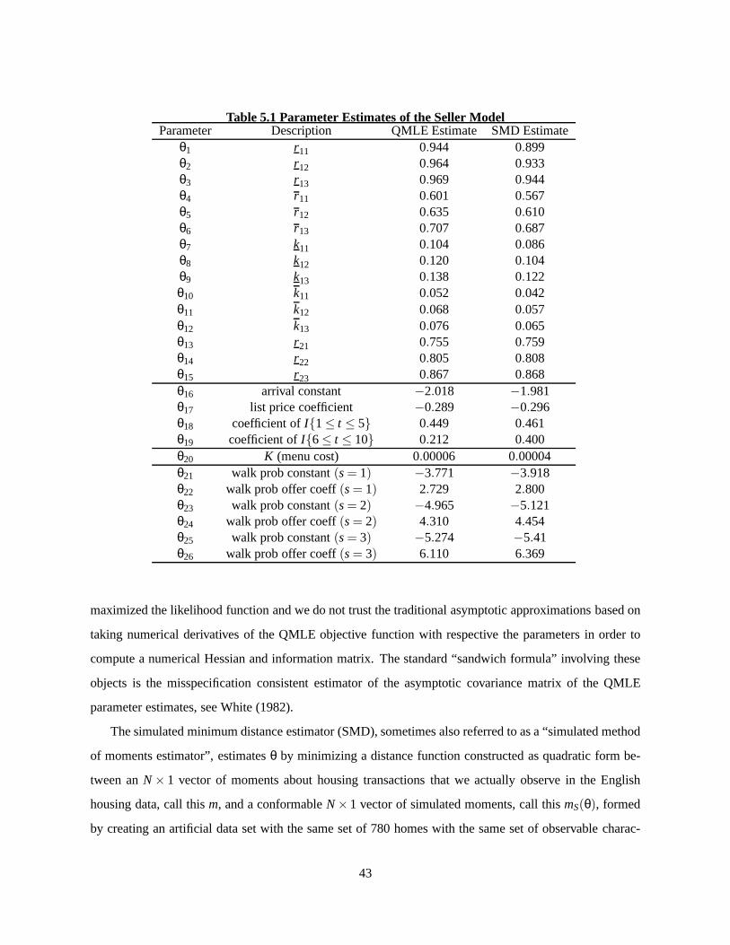
Table 5.1 Parameter Estimates of the Seller ModelParameter Description QMLE Estimate SMD Estimate

θ1 r11 0.944 0.899θ2 r12 0.964 0.933θ3 r13 0.969 0.944θ4 r11 0.601 0.567θ5 r12 0.635 0.610θ6 r13 0.707 0.687θ7 k11 0.104 0.086θ8 k12 0.120 0.104θ9 k13 0.138 0.122θ10 k11 0.052 0.042θ11 k12 0.068 0.057θ12 k13 0.076 0.065θ13 r21 0.755 0.759θ14 r22 0.805 0.808θ15 r23 0.867 0.868θ16 arrival constant −2.018 −1.981θ17 list price coefficient −0.289 −0.296θ18 coefficient ofI{1≤ t ≤ 5} 0.449 0.461θ19 coefficient ofI{6≤ t ≤ 10} 0.212 0.400θ20 K (menu cost) 0.00006 0.00004θ21 walk prob constant(s= 1) −3.771 −3.918θ22 walk prob offer coeff(s= 1) 2.729 2.800θ23 walk prob constant(s= 2) −4.965 −5.121θ24 walk prob offer coeff(s= 2) 4.310 4.454θ25 walk prob constant(s= 3) −5.274 −5.41θ26 walk prob offer coeff(s= 3) 6.110 6.369

maximized the likelihood function and we do not trust the traditional asymptotic approximations based on

taking numerical derivatives of the QMLE objective function with respective the parameters in order to

compute a numerical Hessian and information matrix. The standard “sandwich formula” involving these

objects is the misspecification consistent estimator of theasymptotic covariance matrix of the QMLE

parameter estimates, see White (1982).

The simulated minimum distance estimator (SMD), sometimesalso referred to as a “simulated method

of moments estimator”, estimatesθ by minimizing a distance function constructed as quadraticform be-

tween anN× 1 vector of moments about housing transactions that we actually observe in the English

housing data, call thism, and a conformableN×1 vector of simulated moments, call thismS(θ), formed

by creating an artificial data set with the same set of 780 homes with the same set of observable charac-

43

teristicsX and same hedonic values exp{Xβ} (where theβ coefficients are computed from a first stage

regression using the data, independent of the housing model), but simulatedS times and the individual

moments from eachIID simulation are averaged to form the vector of simulated moments mS(θ). Then

the SMD criterion is

θ = argmin[m−mS(θ)]′W[m−mS(θ)] (27)

whereW is anN×N positive definite weighting matrix. The results we report here are based on a diagonal

weighting matrix so the SMD criterion is equivalent to a formof weighted nonlinear least squares. We

chose the weights so that the moments we consider the most important to try to match are given precedence.

The SMD and QMLE constitute different statistical objective functions so it should not be surprising

that each results in somewhat different parameter estimates. In theory, if the model was correctly specified

and if the global optimum of each of these criteria were obtained, then asymptotically the two different

sets of parameter estimates should converge to the same (true) set of parameter valuesθ∗. However more

realistically our model is likely to be misspecified in important respects and parameters that maximize the

QMLE criterion are not necessarily close to the ones that minimize the SMD criterion. Further, as we

discuss below, both of these objective functions are quite jagged functions of the parameters, and while

we tried diligently to search the 26 dimensional parameter space to ensure that the parameter estimates we

report in Table 5.1 are global and not just not local optimizers, we cannot provide any guarantee that this

is the case.

Despite these caveats, it is reassuring that the two sets of parameters are not far from each other.

This is an independent check on the validity of each of the estimation criteria, since data problems or

programming errors can easily result in problems in the statistical objective functions that can distort the

parameter estimates. The SMD criterion is based on a total ofN = 286 individual moments. We do not

have space here to list all of these moments. A subset of the moments that we used are reported in table 5.2

below, along with the weights we used for each moment. In the results presented in tables 5.1 and 5.2 we

used equal weights of 1 for allN = 286 moments.

While the SMD and QMLE parameter estimates are not dramatically different from each other in

table 5.1, small changes in the parameters can result in fairly big changes in the objective function value.

In part this reflects the lack of smoothness in the estimationcriteria. For example, we used the converged

value of the QMLE estimates in the first column of table 5.1 as the starting values for the SMD estimator.

The value of the SMD criterion at the QMLE parameter estimates was 657836 but the final value that the

44

Nelder Mead (nonsmooth) optimizer located results in a criterion value of 379476. Thus, the algorithm

found substantial improvements in the objective function by changing certain components ofθ in order to

better fit certain moments in our list ofN = 286 “moments of interest.”

Table 5.2 compares a selected subset of 44 of the universe ofN = 286 moments that we used to estimate

the parameters of the seller’s model by SMD. The reader should trust that we have not “cherry picked”

moments that are most favorable to our model, and a table thatcompares the entire set of 286 moments

is available on request. What table 5.2 shows is that the model captures a broad array of features in the

London housing data, not just the stickiness of list prices.Starting with the first moment in table 5.2, we

see that (as promised in section 3) the SMD parameter estimates do satisfy the “rationality constraint” that

the seller’s financial value is an unbiased expectation of the utlimate selling price. The moment compares

the mean of the ratios of the actual sale price for each of the 780 houses sold to the hedonic price exp{Xβ}

(in the Actual Value column) to the mean of the same ratio from5 IID simulations of the model with the

same 780 houses and the same hedonic values, but with the difference being that the simulated transaction

price is generated from our model. We see that the actual moment has a mean of nearly 100%, which is

to be expected given that the hedonic value is by construction an unbiased predictor of the actual sales

price. The fact that the simulated moment is also equal to 1 indicates that the rationality constraint, i.e.

that the financial value is a conditional expectation of the actual sales prices, does hold in our model. To

see this recall that the financial value is given byF = exp{Xβ + η0} whereη0 constitutes unobservables

characteristics of the home. Recall that we assumedη0 to be normal with meanµ and standard deviation

σ, but we constrainedµ such that for any value ofσ, the mean of the lognormally distributed random

variable exp{η0} is 1. This implies that if the hedonic price component of the financial value exp{Xβ} is

an unbiased predictor of the sales price of the home, then so will the financial valueF = exp{Xβ+η0}. We

regard the fact that the best fitting parameter estimates “automatically” enforce the rationality constraint

(without us having to impose it) is further evidence in favorof hypothesis that the selling behavior that we

observe in the English housing data can be well approximatedby a model of rational sellers.

The second row of table 5.2 compares the standard deviation of the ratio of sale price to the hedonic

value and the fact that these standard deviations are close is another way of saying that the model captures

the overall dispersion of sales prices, not just the mean value. In fact the model provides an extremely

accurate approximation of theinitial distribution of list prices in addition to the final sales price.

Rows 3-6 of table 5.2 show that the model does a good job of capturing the price stickiness: it closely

45

matches the fraction of sales which involved no list price changes and 1 list price change. The model

slightly overpredicts the fraction of homes that have 2 or more list price changes, but this can be improved

by increasing the size of the menu cost slightly. Note from table 5.1 that the SMD estimate of the menu

cost of changing list prices isK = 0.00004, which is only 2/3 of the QMLE estimate of this value.

Rows 7-9 of table 5.2 show that the model does not do quite as well in terms of matching the fraction

of accepted offers equal to, below, and above the list price.The model predicts that 26% of all sales

should be at the list price, which is higher than the 15% valuewe observe in the English housing data.

The model underpredicts the number of transactions that occur below the list price (64% versus 81%) and

it underpredicts the fraction of sales that occur above the list price (4% versus 10%). We believe these

predictions can be improved with modest changes to the parameter values that shift the distribution of bids

by buyers, and also the reservation prices charged by sellers. Overall, we think the model is generally in

the “ballpark” of what we observe in the data, however.

Rows 11-14 of table 5.2 show that the simple binomial logit model of arrival rates provides a good

overall approximation to the number of matches (i.e. offers) made on homes. The mean number of

matches in the simulated data, 1.44, is just modestly higher than the mean number of matches weobserve

in the data, 1.34. Rows 16-18 show that the model also generally approximates the non-stationary pattern

of arrival rates, with a significantly higher arrival rate ofmatches in weeks 2-5 and 6-10.

Rows 19-27 show that the model provides a reasonably good prediction of the mean duration to sale

and the survival function of unsold homes at various durations after the initial listing. In general, the

survival function from the model is slightly higher than we observe in the data, and this higher survival

function implies a higher duration to sale in the model (12 weeks) compared to what we observe in the data

(10 weeks). Again, we believe it is possible to improve the fitof the model by small adjustments to the

parameters that result in a faster rate of decline in the seller’s reservation prices relative to bids made by

buyers. The equal weighting of allN = 286 moments in our initial SMD estimates in table 5.1 placed more

importance on fitting moments we consider less important than moments in rows 19-27, so by increasing

the weights on these moments (and other moments in table 5.2 we consider especially important), we

expect a revised version of the SMD estimates will result in substantially better fits than we report here.

Rows 28-30 of table 5.2 show that while the model does accurately approximate the mean time to the

first match, it substantially overpredicts the mean durations to the 2nd and 3rd matches. This could be a

sign of “clustering” in matches that our model does not currently account for. Recall that our formulation

46

of the seller model allows the duration since last offerdt to be a state variable in the model. We did not

actually use this state variable in the version of the model reported here. By including this duration we can

capture the clustering phenomenon by allowing the offer arrival rates to be elevated in the weeks following

a previous match. This would enable the model to better approximate the mean times to a 2nd and 3rd

match.

Rows 31-34 of table 5.2 show that the model is generally able to track the dynamics of list price

markups and reductions as a function of duration on the market. The model predicts a somewhat lower

initial markup of the list price over the hedonic value than we observe in the data (1.04 versus 1.05),

but both the simulated and actual trajectories provide the additional evidence of list price stickiness, and

confirm the model’s ability to capture this key feature of thedata.

Rows 35-39 show that our piecewise linear model of bidding behavior and the assumed beta distribu-

tion of buyer valuations provide a good approximation to bidding behavior. The mean ratio of the first offer

to the list price in the data is 94% versus 93% in our model. Themodel overpredicts the fraction of first

bids equal to the list price (16% versus 10%), but this can be remedied by reducing the length of the flat

segment of the bidding function at the list price. Conversely the model somewhat underpredicts the frac-

tion of first offers that are below the list price and overpredicts the fraction of first offers that are above the

list price. Further experimentation with the parameters ofthe beta distribution of buyer valuations (which

is currently fixed at the initial values we guessed as discussed above) should result in a substantially better

fit. Row 39 shows that the model predicts that only 27% of all first offers are accepted whereas in the

data we see that nearly 42% of first offers are accepted. We believe that this is another sign that the seller

reservation prices are currently somewhat too high and should fall off at a faster rate with duration on the

market. We know how to fix this issue too, mainly by adjusting our (currently fixed) initial guess for the

holding cost functionht(d).

Rows 40-44 present the same comparison, but for the second offers. We see a rather closer correspon-

dence between the model and the data here, except that the model over predicts the fraction of second

offers that are above the list price. This can be fixed by adjusting the estimates of how buyers adjust

their counteroffers in successive stages of the bargainingsubgame. The current estimates suggest that our

model has buyers being somewhat too aggressive in improvingtheir counteroffer in response to an initial

rejection by the seller.

47

6 Implications of the Model

Not yet written up: to be presented in the seminar

7 Conclusions

Not yet written up: to be presented in the seminar

48

References

[1] Albrecht, J., A. Anderson, E. Smith and S. Vroman (2006) “Opportunistic Matching in the HousingMarket” manuscript, Georgetown University.

[2] Anglin, P.M., R. Rutherford, and T.A. Springer (2003) “The trade-off between the selling price ofresidential properties and the time-on-the-market”Journal of Real Estate Finance and Economics2695–111.

[3] Arnold, M.A. (1999) “Search, bargaining and optimal asking prices”Real Estate Economics27453–482.

[4] Bayer, P., R. McMillan, A. Murphy and C. Timmins (2007) “ADynamic Model of the HousingMarket” manuscript, Duke University.

[5] Bowman, D., Minehart, D. and M. Rabin (1999) “Loss aversion in a consumption savings model”Journal of Economic Behavior and Organization38-2155–178.

[6] Brown, J.N. and H.S. Rosen (1982) “On the Estimation of Structural Hedonic Price Models”Econo-metrica50-3765–768.

[7] Carillo, P.E. (2006) “An Empirical Two-sided Equilibrium Search Model of the Real Estate Market”manuscript, George Washington University.

[8] Genesove, D. and C.J. Mayer (1997) “Equity and time to sale in the real estate market”AmericanEconomic Review87255–269.

[9] Genesove, D. and C.J. Mayer (2001) “Loss aversion and seller behavior: Evidence from the housingmarket”Quarterly Journal of Economics1161233–1260.

[10] Glower, M., D.R. Haurin, and P.H. Hendershott (1998) “Selling time and selling price: The influenceof seller motivation”Real Estate Economics26719–740.

[11] D. Haurin (1988) “The duration of marketing time of residential housing”Journal of the AmericanReal Estate and Urban Economics Association16 396–410.

[12] Horowitz, J.L. (1992) “The role of the list price in housing markets: Theory and econometric model”Journal of Applied Econometrics7 115–129.

[13] Kang, H., and M. Gardner, (1989) “Selling Price and Marketing Time in Residential Real EstateMarket” The Journal of Real Estate Research4 21–35.

[14] Kahneman, D. and A. Tversky (1979) “Prospect Theory: AnAnalysis of Decision under Risk”Econometrica48263–291.

[15] J.R. Knight, C.F. Sirmans, and G.K. Turnbull, (1998) “List price information in residential appraisaland underwriting”Journal of Real Estate Research15 59–76.

[16] Knight, J.R. (2002) “Listing price, time on market, andultimate selling price: Causes and effects oflisting price changes”Real Estate Economics30 213–237.

49

[17] Levitt, Steven D. and Chad Syverson (2002) “Market Distortions when Agents are Better Informed:A Theoretical and Empirical Exploration of the Value of Information in Real Estate Transactions”University of Chicago, mimeo.

[18] Miller, N.G. and M.A. Sklarz (1987) “Pricing strategies and residential property selling prices”TheJournal of Real Estate Research2 31–40.

[19] Merlo, A. and F. Ortalo-Magne (2004) “Bargaining over Residential Real Estate: Evidence fromEngland”Journal of Urban Economics56 192–216.

[20] Rust, J. (1988) “Maximum Likelihood Estimation of Discrete Control Processes”SIAM Journal onControl and Optimization26-5, 1006-1024.

[21] Springer, T.E. (1996) “Single family housing transactions: Seller motivations, price and marketingtime” Journal of Real Estate Finance and Economics13 237–254.

[22] Salant, S.W. (1991) “For Sale by Owner: When to Use a Broker and How to Price the House”Journalof Real Estate Finance and Economics4 157–173.

[23] Taylor, C.R. (1999) “Time-on-the-market as a sign of quality” Review of Economic Studies66 555–578.

[24] Yavas, A. (1992) “A simple search and bargaining modelof real estate markets”Journal of theAmerican Real Estate and Urban Economics Association20 533–548.

[25] Yavas, A. and S. Yang (1995) “The strategic role of listing price in marketing real estate: Theory andevidence”Real Estate Economics23347–368.

[26] Wheaton, W.C. and G. Nechayev (2006) “Past Housing ‘Cycles’ and the Current Housing ‘Boom’:Whats Different This Time?” manuscript, Massachusetts Institute of Technology.

[27] White, H. (1982) “Maximum Likelihood Estimation of Misspecified Models”Econometrica501–25.

[28] Witte, A.D., H.J. Sumka and H. Erekson (1979) “An Estimate of a Structural Hedonic Price Modelof the Housing Market: An Application of Rosen’s Theory of Implicit Markets” Econometrica471151–1173.

[29] Zuehlke, T.W. (1987) “Duration dependence in the housing market”The Review of Economics andStatistics69 701–704.

[30] Zumpano, L., K. Johnson, and R. Anderson (2003) “Internet use and real estate brokerage marketintermediation”Journal of Housing Economics12 134–150.

50

Table 5.2 Actual and Simulated MomentsMoment Actual Value Simulated Value1 mean sale price/hedonic price ratio 99.7 100.52 standard deviation of sale price/hedonic price ratio 29.9 31.23 % of homes with no list price changes 77.3 76.44 % of homes with 1 list price change 20.7 20.25 % of homes with 2 list price changes 1.9 2.96 % of homes with 3+ list price changes 0.0 0.57 % of accepted offers equal to list price 15.2 268 % of accepted offers below list price 80.7 63.69 % of accepted offers above list price 10.4 4.010 % of homes never sold 0.0 0.0711 % of homes with no matches 0.0 0.012 % of homes with 1 match 76.7 72.613 % of homes with 2 matches 17.9 21.214 % of homes with 3+ matches 5.4 6.215 Mean number of matches 1.44 1.3416 Prob of match in week 1 10.7 9.217 Prob of match in weeks 2-5 15.8 13.718 Prob of match in weeks 6-10 13.4 12.819 Mean duration to sale (weeks) 10.3 12.020 % of homes unsold after 2 weeks 92.4 94.121 % of homes unsold after 4 weeks 71.0 77.822 % of homes unsold after 8 weeks 44.5 51.723 % of homes unsold after 10 weeks 36.5 42.824 % of homes unsold after 15 weeks 22.7 28.825 % of homes unsold after 20 weeks 14.7 20.226 % of homes unsold after 26 weeks 10.6 12.227 % of homes unsold after 40 weeks 2.8 3.628 Mean time to first match 8.9 8.729 Mean time to second match 4.5 9.230 Mean time to third match 4.7 10.031 Mean list/hedonic price ratio at list 105.0 103.532 Mean list/hedonic price ratio at week 5 105.2 103.533 Mean list/hedonic price ratio at week 10 104.0 103.434 Mean list/hedonic price ratio at week 20 101.6 102.235 Mean first offer/list price 94.0 93.436 % of first offers equal to list 10.1 15.937 % of first offers below list 87.2 76.438 % of first offers above list 2.6 7.639 % of first offers accepted 41.6 27.040 Mean second offer/list price 95.6 94.041 % of second offers equal to list 7.6 5.842 % of second offers below list 88.6 85.043 % of second offers above list 3.8 9.144 % of second offers accepted 54.7 59.7

51