1

1. Plate Tectonics defined.

3. Alfred Wegener and Continental Drift.EvidenceTheoryOutcome

2. What did Plate Tectonics replace?

The History of Continental Drift Plate: The Earth’s crust consists of a number of mobile plates, masses of crust that move independently of adjacent plates.

Tectonics: dealing with structural features of the Earth (e.g., mountains, ocean basins).

Plate Tectonics: The process that involves the interaction of moving crustal plates and results in major structural features of the Earth.

A unifying theory in geology that explains a wide range of geologic phenomena.

What did the modern theory replace?

Diastrophism: early term for all movement of the Earth’s crust.

•Thought to result in the formation of mountains, ocean basins, etc.

Contracting Earth Theory

•Theory that the Earth contracted or shrank over geologic time.

• Shrinking resulted in a reduction in the Earth’s diameter while the circumference remained unchanged due to folding and buckling of the crust (diastrophism).

•First proposed by Giordano Bruno (16th C) who compared the process to the drying of an apple.

Lord Kelvin (19th C) suggested that contraction was due to cooling of the Earth.

The problems with this mechanism:

•Fossils are preserved in rocks that represent organisms that could not withstand the early temperatures.

•Initial temperatures required for the amount of contraction were too high to be realistic.

2

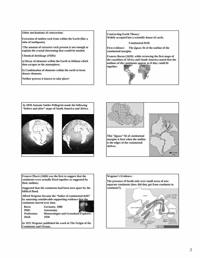
Other mechanisms of contraction:

Extrusion of molten rock from within the Earth (like a tube of toothpaste).

•The amount of extrusive rock present is not enough to explain the crustal shortening that would be needed.

Chemical shrinkage (1920s)

a) Decay of elements within the Earth to Helium which then escapes to the atmosphere.

b) Combination of elements within the earth to form denser elements.

Neither process is known to take place!

Contracting Earth Theory: Widely accepted but a scientific house of cards.

Continental Drift

First evidence: The jigsaw fit of the outline of the continental margins.

Frances Bacon (1620): while reviewing the first maps of the coastlines of Africa and South America noted that the outlines of the continents appear as if they could fit together.

In 1858 Antonio Snider-Pellegrini made the following “before and after” maps of South America and Africa.

This “jigsaw” fit of continental margins is best when the outline is the edges of the continental shelves.

Frances Placet (1668) was the first to suggest that the continents were actually fixed together as suggested by their outlines.

Suggested that the continents had been torn apart by the biblical flood.

Born: Germany, 1880PhD: AstronomyProfession: Meteorologist and Greenland Explorer.Died: 1930

Alfred Wegener became the “father of continental drift”by amassing considerable supporting evidence that the continents moved over time.

In 1915 Wegener published his work in The Origin of the Continents and Oceans.

Wegener’s Evidence:

The presence of fossils only over small areas of now separate continents (how did they get from continent to continent?).

3

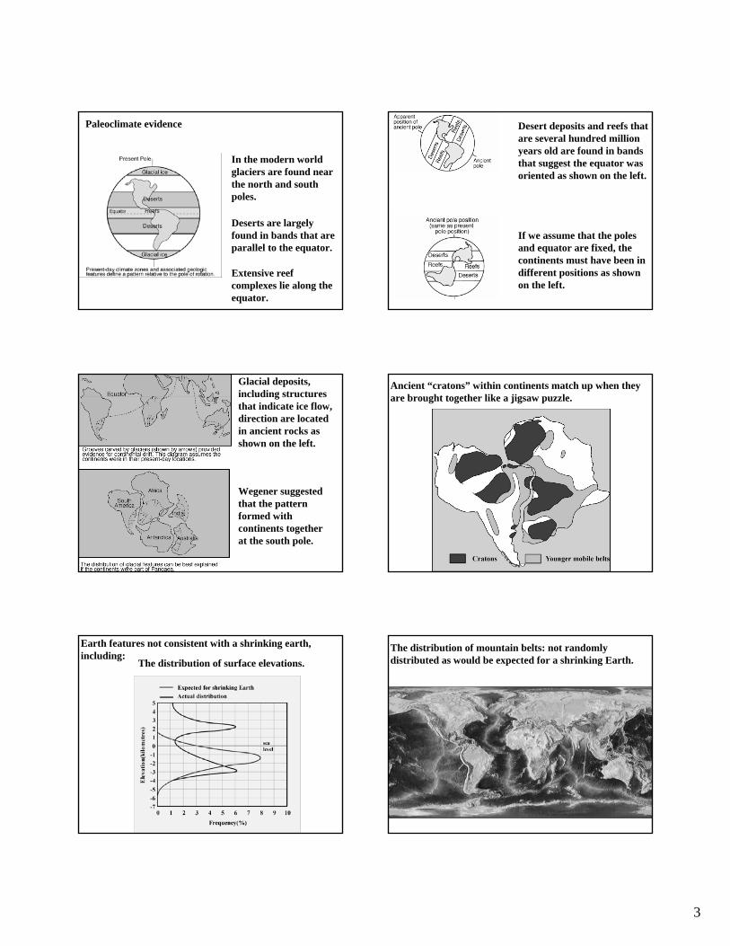
Paleoclimate evidence

In the modern world glaciers are found near the north and south poles.

Deserts are largely found in bands that are parallel to the equator.

Extensive reef complexes lie along the equator.

Desert deposits and reefs that are several hundred million years old are found in bands that suggest the equator was oriented as shown on the left.

If we assume that the poles and equator are fixed, the continents must have been in different positions as shown on the left.

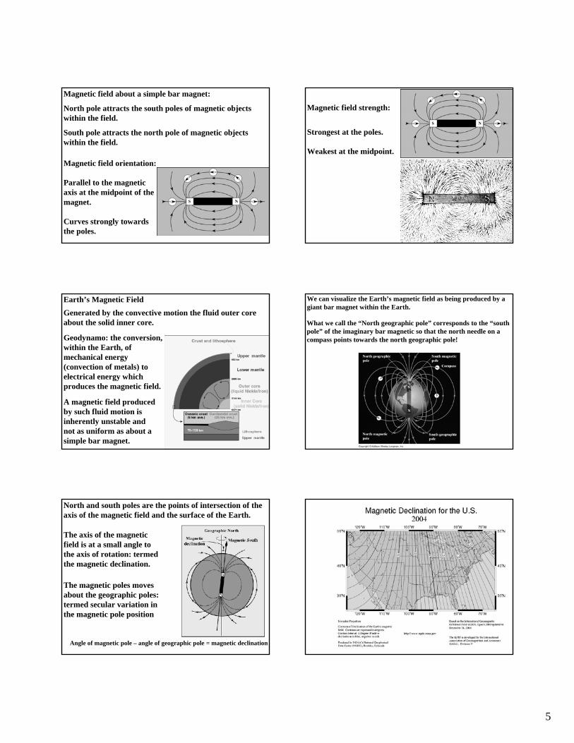
Glacial deposits, including structures that indicate ice flow, direction are located in ancient rocks as shown on the left.

Wegener suggested that the pattern formed with continents together at the south pole.

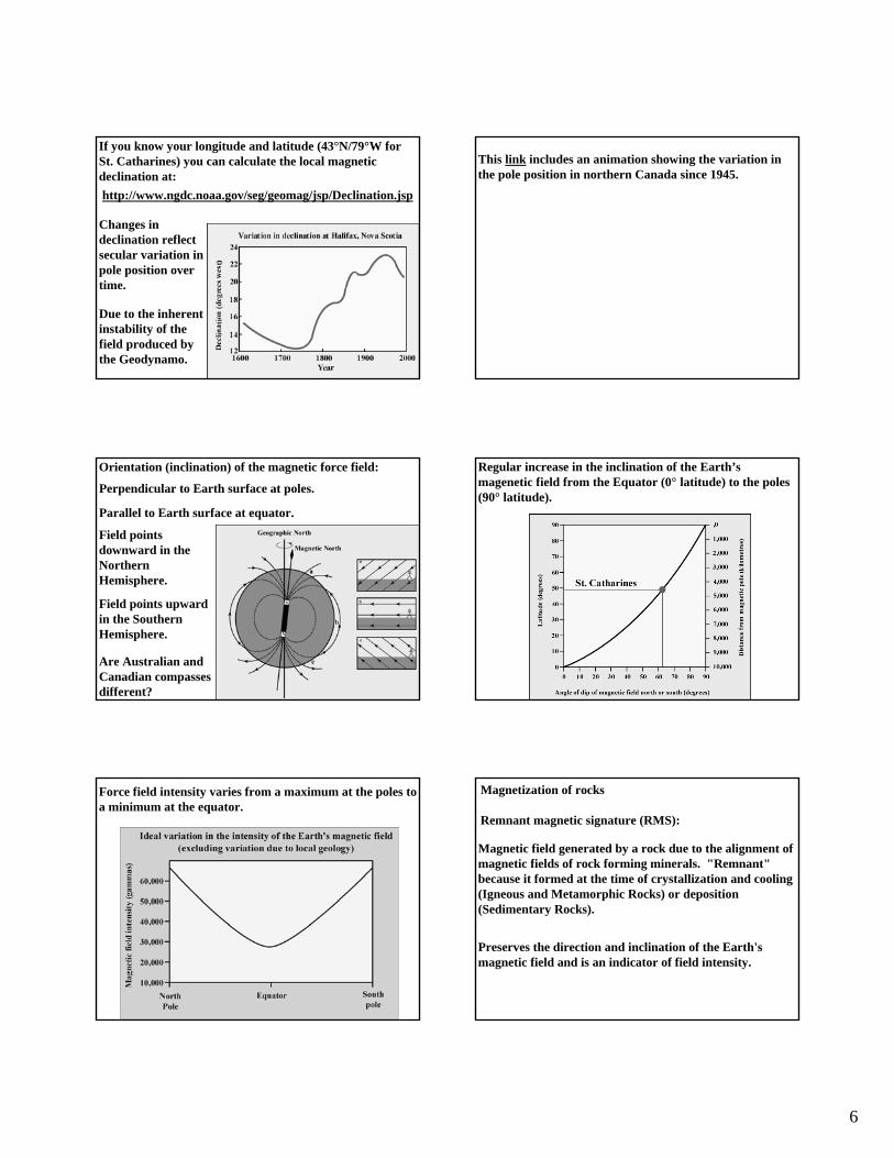
Ancient “cratons” within continents match up when they are brought together like a jigsaw puzzle.

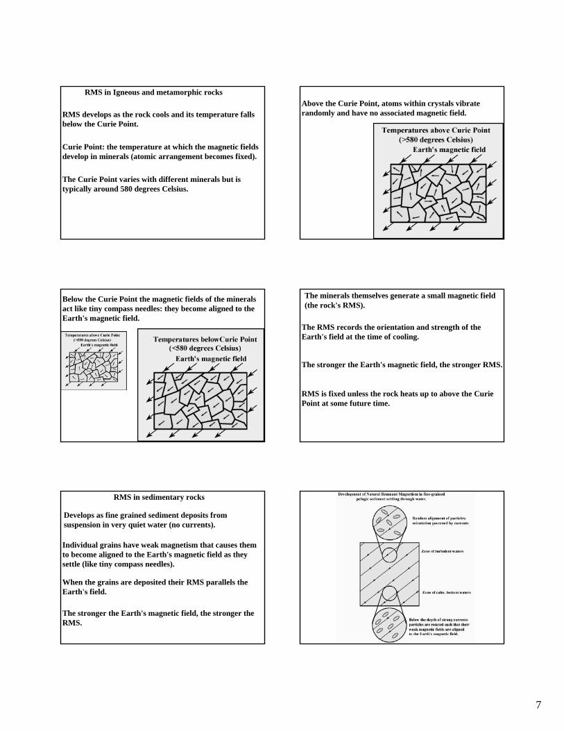
Earth features not consistent with a shrinking earth, including:

The distribution of surface elevations.The distribution of mountain belts: not randomly distributed as would be expected for a shrinking Earth.

4

Wegener’s Conclusions:

1. That the continents were once joined. Therefore, they must have moved apart over time.

2. Contracting Earth theory was not consistent with the facts.

Wegener proposed a mechanism for continental drift: pushing of the continents by gravitational forces that derived from the sun and the moon (similar to tides).

Wegener’s ideas were strongly challenged by the scientific community.They suggested alternative interpretations of his paleontological data:

Paleoclimate evidence was explained movement of the poles rather than the continents.

Other evidence was refuted as being “coincidence” or just being incorrect.

Errors in Wegener’s data led to easy arguments against some conclusions.

He had predicted the North America and Europe were moving away from each other at the rate of 250 cm/year……an impossible rate.

(we now know that they are moving apart at a rate up to 3 cm per year)

The second Biggest problem: the mechanism that Wegener proposed was impossible and easily demonstrated to be so.

By 1930 there were few geologists who believed Wegener’shypothesis.

He died while on an expedition to Greenland, two days after his 50th birthday.

Over the next 20 years any suggestion of moving continents was received with strong opposition.

In the 1950s evidence from the geological record of the Earth’s magnetic field began to strongly suggest exactly such movement.

The biggest problem was that Wegener’s ideas were contrary to the dogma of the day.

Geomagnetism

The Earth’s Magnetic field.

Magnetization of rocks

The Earth’s magnetic record

Proof of continental drift© C Gary A. GlatzmaierUniversity of California, Santa Cruz

Magnetism

Magnetic Force field:The region around a magnetic object in which its magnetic forces act on other magnetic objects.

5

Magnetic field about a simple bar magnet:

North pole attracts the south poles of magnetic objects within the field.

South pole attracts the north pole of magnetic objects within the field.

Magnetic field orientation:

Parallel to the magnetic axis at the midpoint of the magnet.

Curves strongly towards the poles.

Magnetic field strength:

Strongest at the poles.

Weakest at the midpoint.

Earth’s Magnetic FieldGenerated by the convective motion the fluid outer core about the solid inner core.

Geodynamo: the conversion, within the Earth, of mechanical energy (convection of metals) to electrical energy which produces the magnetic field.

A magnetic field produced by such fluid motion is inherently unstable and not as uniform as about a simple bar magnet.

What we call the “North geographic pole” corresponds to the “south pole” of the imaginary bar magnetic so that the north needle on a compass points towards the north geographic pole!

We can visualize the Earth’s magnetic field as being produced by a giant bar magnet within the Earth.

Angle of magnetic pole – angle of geographic pole = magnetic declination

North and south poles are the points of intersection of the axis of the magnetic field and the surface of the Earth.

The axis of the magnetic field is at a small angle to the axis of rotation: termed the magnetic declination.

The magnetic poles moves about the geographic poles: termed secular variation in the magnetic pole position

6

If you know your longitude and latitude (43°N/79°W for St. Catharines) you can calculate the local magnetic declination at:

Changes in declination reflect secular variation in pole position over time.

Due to the inherent instability of the field produced by the Geodynamo.

http://www.ngdc.noaa.gov/seg/geomag/jsp/Declination.jsp

This link includes an animation showing the variation in the pole position in northern Canada since 1945.

Orientation (inclination) of the magnetic force field:

Parallel to Earth surface at equator.

Perpendicular to Earth surface at poles.

Field points downward in the Northern Hemisphere.

Field points upward in the Southern Hemisphere.

Are Australian and Canadian compasses different?

Regular increase in the inclination of the Earth’s magenetic field from the Equator (0° latitude) to the poles (90° latitude).

Force field intensity varies from a maximum at the poles to a minimum at the equator.

Magnetization of rocks

Remnant magnetic signature (RMS):

Magnetic field generated by a rock due to the alignment of magnetic fields of rock forming minerals. "Remnant" because it formed at the time of crystallization and cooling (Igneous and Metamorphic Rocks) or deposition (Sedimentary Rocks).

Preserves the direction and inclination of the Earth's magnetic field and is an indicator of field intensity.

7

RMS in Igneous and metamorphic rocks

RMS develops as the rock cools and its temperature falls below the Curie Point.

Curie Point: the temperature at which the magnetic fields develop in minerals (atomic arrangement becomes fixed).

The Curie Point varies with different minerals but is typically around 580 degrees Celsius.

Above the Curie Point, atoms within crystals vibrate randomly and have no associated magnetic field.

Below the Curie Point the magnetic fields of the minerals act like tiny compass needles: they become aligned to the Earth's magnetic field.

The minerals themselves generate a small magnetic field (the rock's RMS).

The RMS records the orientation and strength of the Earth's field at the time of cooling.

The stronger the Earth's magnetic field, the stronger RMS.

RMS is fixed unless the rock heats up to above the Curie Point at some future time.

RMS in sedimentary rocks

Develops as fine grained sediment deposits from suspension in very quiet water (no currents).

Individual grains have weak magnetism that causes them to become aligned to the Earth's magnetic field as they settle (like tiny compass needles).

When the grains are deposited their RMS parallels the Earth's field.

The stronger the Earth's magnetic field, the stronger the RMS.

8

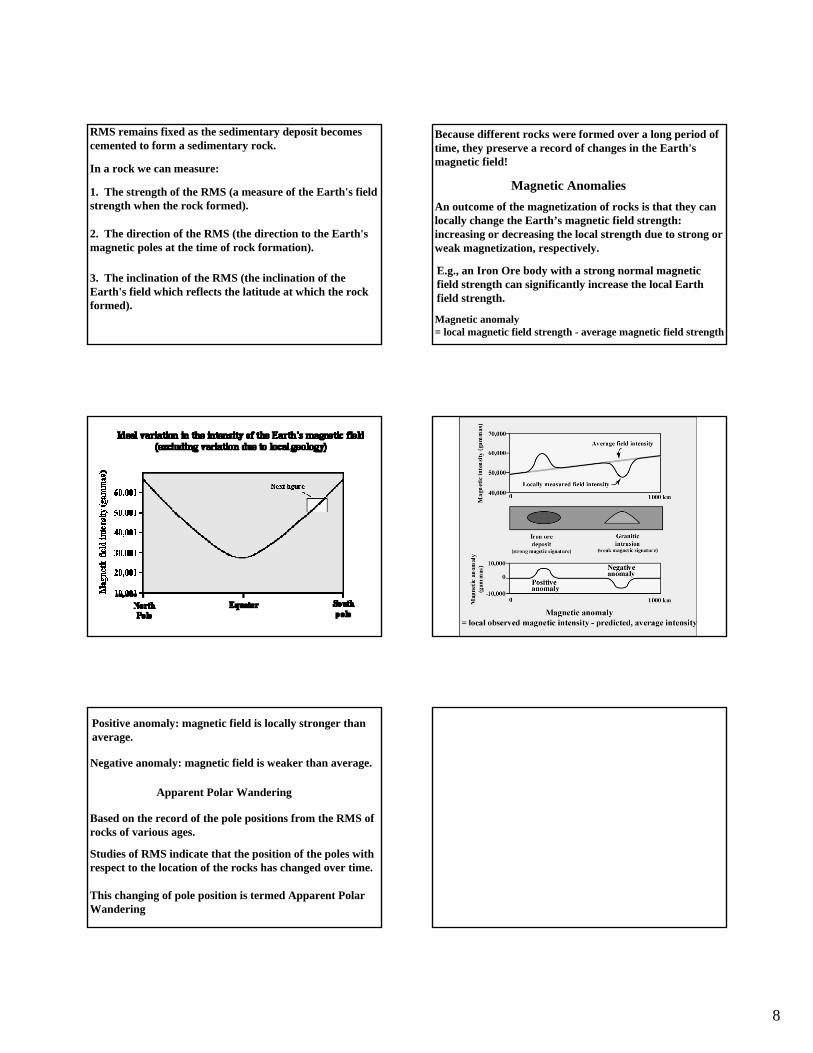
RMS remains fixed as the sedimentary deposit becomes cemented to form a sedimentary rock.

In a rock we can measure:

1. The strength of the RMS (a measure of the Earth's field strength when the rock formed).

2. The direction of the RMS (the direction to the Earth's magnetic poles at the time of rock formation).

3. The inclination of the RMS (the inclination of the Earth's field which reflects the latitude at which the rock formed).

Because different rocks were formed over a long period of time, they preserve a record of changes in the Earth's magnetic field!

An outcome of the magnetization of rocks is that they can locally change the Earth’s magnetic field strength: increasing or decreasing the local strength due to strong or weak magnetization, respectively.

E.g., an Iron Ore body with a strong normal magnetic field strength can significantly increase the local Earth field strength.

Magnetic Anomalies

Magnetic anomaly= local magnetic field strength - average magnetic field strength

Positive anomaly: magnetic field is locally stronger than average.

Negative anomaly: magnetic field is weaker than average.

Apparent Polar Wandering

Based on the record of the pole positions from the RMS of rocks of various ages.

Studies of RMS indicate that the position of the poles with respect to the location of the rocks has changed over time.

This changing of pole position is termed Apparent Polar Wandering

9

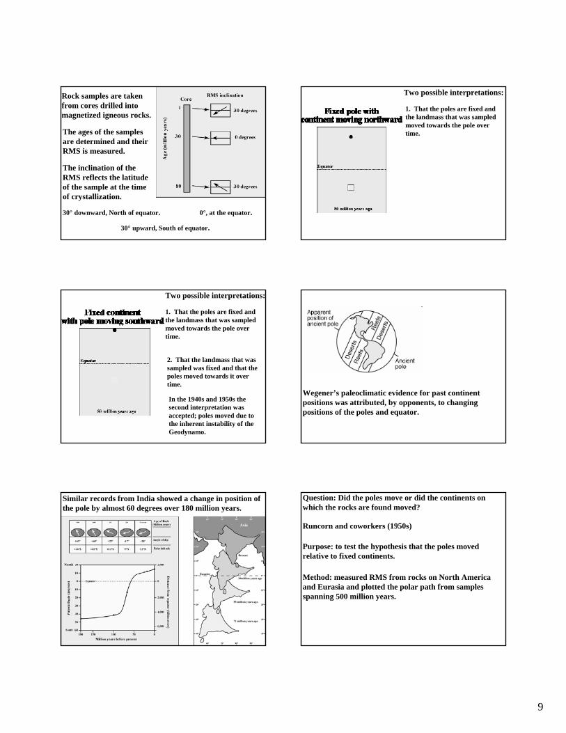
Rock samples are taken from cores drilled into magnetized igneous rocks.

The ages of the samples are determined and their RMS is measured.

The inclination of the RMS reflects the latitude of the sample at the time of crystallization.

30° downward, North of equator. 0°, at the equator.

30° upward, South of equator.

1. That the poles are fixed and the landmass that was sampled moved towards the pole over time.

Two possible interpretations:

2. That the landmass that was sampled was fixed and that the poles moved towards it over time.

In the 1940s and 1950s the second interpretation was accepted; poles moved due to the inherent instability of the Geodynamo.

1. That the poles are fixed and the landmass that was sampled moved towards the pole over time.

Two possible interpretations:

Wegener’s paleoclimatic evidence for past continent positions was attributed, by opponents, to changing positions of the poles and equator.

Similar records from India showed a change in position of the pole by almost 60 degrees over 180 million years.

Question: Did the poles move or did the continents on which the rocks are found moved?

Runcorn and coworkers (1950s)

Purpose: to test the hypothesis that the poles moved relative to fixed continents.

Method: measured RMS from rocks on North America and Eurasia and plotted the polar path from samples spanning 500 million years.

10

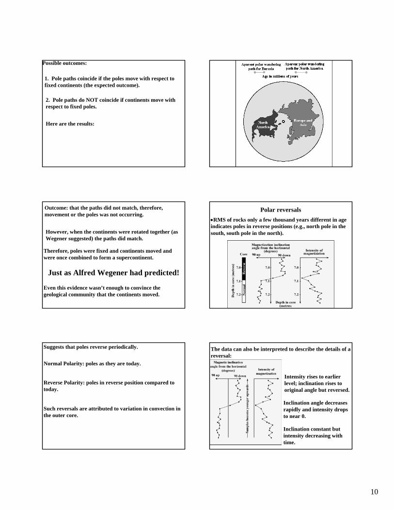
Possible outcomes:

1. Pole paths coincide if the poles move with respect to fixed continents (the expected outcome).

2. Pole paths do NOT coincide if continents move with respect to fixed poles.

Here are the results:

Outcome: that the paths did not match, therefore, movement or the poles was not occurring.

Just as Alfred Wegener had predicted!

Even this evidence wasn’t enough to convince the geological community that the continents moved.

However, when the continents were rotated together (as Wegener suggested) the paths did match.

Therefore, poles were fixed and continents moved andwere once combined to form a supercontinent.

Polar reversals•RMS of rocks only a few thousand years different in age indicates poles in reverse positions (e.g., north pole in the south, south pole in the north).

Suggests that poles reverse periodically.

Normal Polarity: poles as they are today.

Reverse Polarity: poles in reverse position compared to today.

Such reversals are attributed to variation in convection in the outer core.

The data can also be interpreted to describe the details of a reversal:

Inclination constant but intensity decreasing with time.

Inclination angle decreases rapidly and intensity drops to near 0.

Intensity rises to earlier level; inclination rises to original angle but reversed.

11

Actual “flipping”of the poles takes only 1000-2000 years.

The field is lost as the intensity drops to 0; it comes back with flipped poles.

A reversal takes a total of 10 to 20 thousand years*.

*The last reversal took 1000 years at the equator but 10,000 years at midlatitudes.

Animation from :http://www.psc.edu/science/Glatzmaier/glatzmaier.html(click here to access this site)

Polar reversal animation

Yellow = north pole.

Blue = south pole.

Due to the inherent instability of the geodynamo.

Over long periods of geologic time the poles have reversed thousands of times.Certain periods of geologic time are

dominated by normal or reversed polarity whereas others are periods of mixed polarity.

We live in a period when polarity is reversing, on average, every 250,000 years.

Over the past 600 million years the time between reversals varied from 5,000 years to 50 million years.

Is the Earth’s magnetic field polarity currently reversing?

The last polar reversal took place nearly 800,000 years ago

We are overdue given the average time between reversals over the past several millions of years.

Evidence for a decline in magnetic field intensity:

6.4% reduction in intensityOver 100 years.

Extrapolating the current trend to the future suggests that the field intensity will reach zero in approximately 1500 years (i.e., the poles will reverse).

12

Do polar reversals pose a threat to life on Earth?

The “magnetosphere” shields the Earth from high energy particles from the Sun.

As the intensity of the field decreases through a reversal the magnetosphere becomes less and less effective in reducing solar radiation.

Earth’s atmosphere also acts as a shield to such particles.

There is no evidence that the loss of the magnetosphere leads to harm to any life on Earth.

Magnetosphere animation

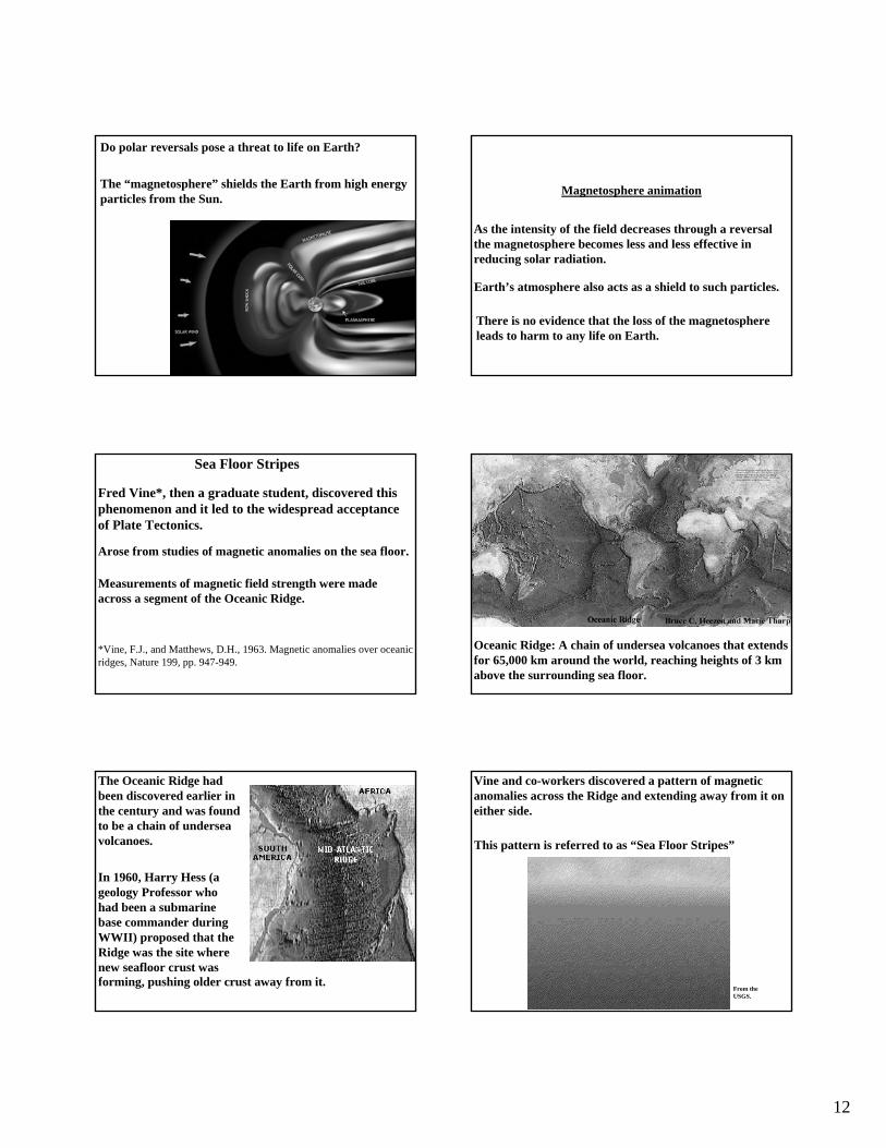
Sea Floor Stripes

Arose from studies of magnetic anomalies on the sea floor.

Measurements of magnetic field strength were made across a segment of the Oceanic Ridge.

Fred Vine*, then a graduate student, discovered this phenomenon and it led to the widespread acceptance of Plate Tectonics.

*Vine, F.J., and Matthews, D.H., 1963. Magnetic anomalies over oceanic ridges, Nature 199, pp. 947-949.

Oceanic Ridge: A chain of undersea volcanoes that extends for 65,000 km around the world, reaching heights of 3 km above the surrounding sea floor.

The Oceanic Ridge had been discovered earlier in the century and was found to be a chain of undersea volcanoes.

In 1960, Harry Hess (a geology Professor who had been a submarine base commander during WWII) proposed that the Ridge was the site where new seafloor crust wasforming, pushing older crust away from it.

This pattern is referred to as “Sea Floor Stripes”

Vine and co-workers discovered a pattern of magnetic anomalies across the Ridge and extending away from it on either side.

From the USGS.

13

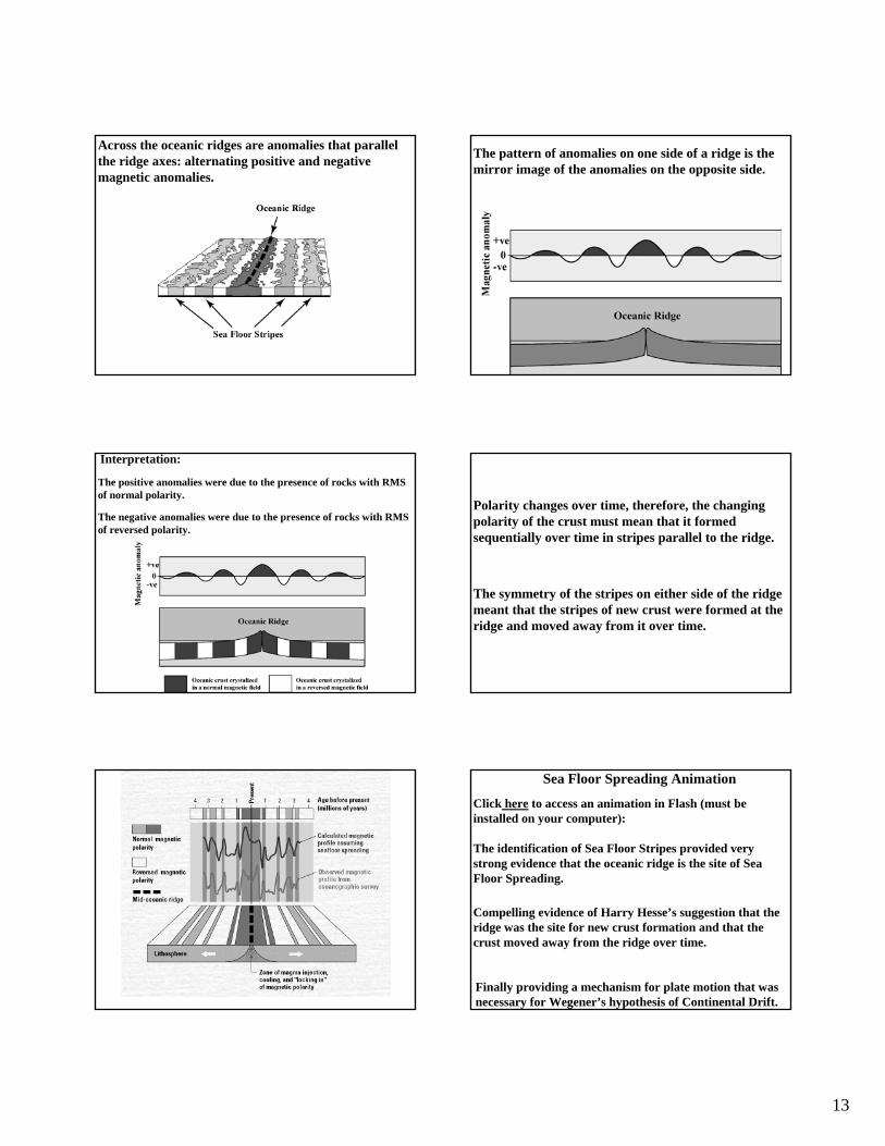
Across the oceanic ridges are anomalies that parallel the ridge axes: alternating positive and negative magnetic anomalies.

The pattern of anomalies on one side of a ridge is the mirror image of the anomalies on the opposite side.

The positive anomalies were due to the presence of rocks with RMS of normal polarity.

The negative anomalies were due to the presence of rocks with RMS of reversed polarity.

Interpretation:

Polarity changes over time, therefore, the changing polarity of the crust must mean that it formed sequentially over time in stripes parallel to the ridge.

The symmetry of the stripes on either side of the ridge meant that the stripes of new crust were formed at the ridge and moved away from it over time.

Sea Floor Spreading Animation

Click here to access an animation in Flash (must be installed on your computer):

The identification of Sea Floor Stripes provided very strong evidence that the oceanic ridge is the site of Sea Floor Spreading.

Compelling evidence of Harry Hesse’s suggestion that the ridge was the site for new crust formation and that the crust moved away from the ridge over time.

Finally providing a mechanism for plate motion that was necessary for Wegener’s hypothesis of Continental Drift.