The Hidden Earth: Visualization of Geologic Features and their Subsurface

Geometry

Michael D. Piburn, Stephen J. Reynolds, Debra E. Leedy, Carla M. McAuliffe, James P. Birk, and Julia K. Johnson

ARIZONA STATE UNIVERSITY

Paper presented at the annual meeting of the National Association for Research in Science Teaching, New Orleans, LA, April 7-10, 2002.

1

ABSTRACT

Geology is among the most visual of the sciences, with spatial reasoning taking

place at various scales and in various contexts. Among the spatial skills required in introductory college geology courses are spatial rotation (rotating objects in one’s mind), and visualization (transforming an object in one’s mind). To assess the role of spatial ability in geology, we designed an experiment using (1) web-based versions of spatial visualization tests, (2) a geospatial test, and (3) multimedia instructional modules built around innovative QuickTime Virtual Reality (QTVR) movies.

Two introductory geology modules were created – visualizing topography and interactive 3D geologic blocks. The topography module was created with Authorware and encouraged students to visualize two-dimensional maps as three-dimensional landscapes. The geologic blocks module was created in FrontPage and covered layers, folds, faults, intrusions, and unconformities. Both modules had accompanying worksheets and handouts to encourage active participation by describing or drawing various features, and both modules concluded with applications that extended concepts learned during the program.

Computer-based versions of paper-based tests were created for this study. Delivering the tests by computer made it possible to remove the verbal cues inherent in the paper-based tests, present animated demonstrations as part of the instructions for the tests, and collect time-to-completion measures on individual items. A comparison of paper-based and computer-based tests revealed significant correlations among measures of spatial orientation, visualization and achievement.

Students in control and experimental sections were administered measures of spatial orientation and visualization, as well as a content-based geospatial examination. All subjects improved significantly in their scores on spatial visualization and the geospatial examination. There was no change in their scores on spatial orientation. Pre-test scores on the visualization and geospatial measures were significantly lower for the experimental than for the control group, while post-test scores were the same. A two-way analysis of variance revealed significant main effects and a significant interaction. The unexpected initial differences between the groups resulted from an uneven gender distribution, with females dominating the experimental group and males the control group. The initial scores of females were lower than those of males, whereas the final scores were the same. This demonstrates that spatial ability can be improved through instruction, that learning of geological content will improve as a result, and that differences in performance between the genders can be eliminated.

2

BACKGROUND

Visual-Spatial Ability The exceptional role of spatial visualization in the work of scientists and mathematicians is well-known. The German chemist August Kekule described how atoms appeared to “dance before his eyes,” and is said to have discovered the structure of the benzene ring by “gazing into a fire and seeing in the flames a ring of atoms looking like a snake eating its own tail (Rieber, 1995).” Roger Shepard (1988) discusses many examples of how spatial visualization was important to the creative imagination of scientists like Einstein, Faraday, Tesla, Watson and Feynmann. The performance of scientists on standard tests of spatial ability is so high that Anne Roe (1961) had to create special measures for her studies of exceptionally creative scientists. Successful science students in high school and college have higher scores on traditional measures of spatial ability than is true of other students of their age and ability (Carter, LaRussa & Bodner, 1987; Pallrand & Seeber, 1984; Piburn, 1980). Despite the obvious importance of spatial visualization to the geological sciences, there are few studies that explore this relationship. Muehlberger and Boyer (1961) found that students’ scores on a standardized visualization test correlated positively with their grades in an undergraduate structural geology course, as well as grades in previously taken geology courses. In a more recent study, Kali and Orion (1996, 1997) reported that the “ability mentally to penetrate a structure,” which they called visual penetration ability (VPA) is highly related to the ability to solve problems on their Geologic Spatial Ability Test (GeoSAT). The exact nature of scientific abilities in the spatial realm is not clear. Spatial ability can be conceived of in a variety of ways, from recognizing rotated figures (Shepard & Metzler, 1971), to disembedding and “restructuring” information from visual arrays (Witkin, Moore, Goodenough & Cox, 1977) to “mental imagery” (Shepard, 1978). It is possible to think of spatial abilities as a cluster of factorially distinct qualities. Studies of traditional measures show that they separate into at least two groups. Spatial orientation (“the ability to perceive spatial patterns or to maintain orientation with respect to objects in space”) and visualization (“the ability to manipulate or transform the image of spatial patterns into other arrangements”) are factorially distinct abilities (Ekstrom, French, Harman & Dermen, 1976). When considered in this way, the contribution of spatial ability to achievement in science is about the same as that of verbal ability (Piburn, 1992). Another way to think about spatial ability has been provided through the work of Howard Gardner (1985). His theory of Multiple Intelligences proposes that spatial intelligence is one of several quite distinct intellectual abilities. These separate intelligences find their greatest expression in the specialized practices of society. He cites, for example, the case of a child in the South Pacific who has exceptional spatial abilities, and is specially trained for a career as a navigator. Presumably, there has been some kind of a similar tacit program in our culture that has resulted in those with similar abilities being identified and trained as scientists and mathematicians.

3

One of the discouraging results of much of this literature is that, although the importance of spatial abilities is clear, the correlations between the results of spatial measures and achievement in science class are low. One possible explanation for this comes from the study of expertise. Expert performance, it turns out, is very context specific. Chess players can remember more than 50,000 meaningful chess positions, but are no more able than others to remember the random positioning of chess pieces on a board. Expert map-makers have an incredible visual memory for maps, but no better memory than others for other kinds of displays (Ericsson & Smith, 1991). It is a reasonable hypothesis that the correlations would rise substantially if the measures of spatial ability were more closely aligned with the specific science content that was being tested. Some recent proposals in cognitive science and education seem to reflect the idea that knowledge is contextual. These include Anchored Instruction (The Cognition and Technology Group at Vanderbilt, 1990), Problem-Based Learning (Albanese & Mitchell, 1993) and Situated Cognition (Brown, Collins & Duguid, 1989). These three psychological and educational models are similar insofar as they suggest that learning occurs best in situations that are complex, problem-based, realistic and reflective of the actual content of instruction. Very few of these have been attempted in science education, and even fewer in the earth sciences. However, Smith and Hoersch (1995) have reported on the application of problem-based learning in the college geology classroom, including tectonics, mineralogy and metamorphic petrology. They conclude that it “seems more effective than didactic learning at overturning incorrect preconceptions and encouraging interdisciplinary integration of content, independent learning, and active student participation.” Spatial Visualization in Geology

Practicing geologists engage in many kinds of spatial-visual activities. Much of classical geology is concerned with understanding the distribution, both on the surface and at depth, of geologic units, geologic structures, and natural resources. To help them visualize these distributions, geologists have developed various kinds of maps, diagrams, and other graphical representations of geologic data (Rudwick, 1976; Davis and Reynolds, 1996). Geologists use these types of illustrations to help them visualize landscapes, surficial and subsurface geology, and geologic changes over time.

Geologists use topographic maps to visualize the shape of the land surface from the contours. To do this, a geologist must mentally transform the abstract, two-dimensional map, with its squiggly contour lines, into a three-dimensional landscape. Geologists perform a similar spatial transformation by visualizing the landscape from a two-dimensional aerial photograph. In this case, geologists use visual clues from the aerial photo, such as shadows, the typical appearance of streams and other features, and a mental picture of what the landscape “ought to look like.”

Geologists rely extensively on geologic maps, which show the types and ages of rock units exposed on the surface, as well as faults, folds, and other geologic structures. Most geologic maps incorporate a topographic base map so that geologic features can be referenced to their actual elevation and location on the map. A geologist examining a geologic map will alternately focus on the geology and the topography to gain a mental

4

picture of how the two are related. This mental process is a type of disembedding, in which one aspect is mentally isolated from a multifaceted context.

From a geologic map, geologists may construct a geologic cross section, which is an interpretation of the subsurface geology from one point to another. A cross section is like cutting a big slice through the landscape, picking it up, and looking at it from the side, in the same way we look at layers inside a cake. Geologists use cross sections to visualize the subsurface geology and to explore for natural resources by determining the depth to a specific coal-bearing layer, copper deposit, or oil field.

Geologists also construct a sequence of diagrams to illustrate successive geologic changes in an area. Many geologic processes require so much time that humans are not around long enough to observe any changes in the landscape. To approach this problem, geologists have developed the technique of “trading location for time.” By this it is meant that geologists look at several present-day areas and mentally arrange these into a sequence interpreted to represent an evolutionary sequence through time. A narrow deep canyon, for example, is interpreted to be a younger phase of landscape development than an area that has been eroded down into a series of low, subdued hills. Spatial Visualization in Geology Courses

One of the main goals of a geology course is to teach students how to visualize geology in a way similar to practicing geologists. When the laboratory for Introductory Geology was redesigned, a decision was made to restrict the course to those aspects that are most important to real geologists. Students now learn how to:

� construct, read, and visualize topographic and geologic maps, � visualize geology in the subsurface, � visualize and reconstruct past environments from rocks and minerals, � reconstruct geologic history from rocks, minerals, and maps, and � understand the implications of geology for society.

To help students understand and visualize topographic maps, they construct a contour map by successively filling with water a plastic box containing a plastic mountain and drawing a map of the shoreline at each water level. After they have used such concrete manipulatives, the students interact on the computer with a module entitled Visualizing Topography. This experience is reinforced by having students use topographic maps throughout the semester to locate rock and mineral samples and decide which areas have safe slopes for situating a colony.

To help students understand and visualize geologic maps, they construct their own geologic map, on a topographic base, from three-dimensional perspectives of a computer-generated terrain called Painted Canyon (see front cover). To complete this map, students need to (1) recognize how geology and topography interact, (2) draw lines on the topographic map that correspond to boundaries between geologic units on the perspectives, and (3) reconstruct the order in which the rock units and geologic structures were formed. The students then use this geologic map to construct a cross section of the units in the subsurface and to determine the impacts of geology on a colony they must site.

Students then have a chance to apply these skills to several interesting real places. They use topographic maps, geologic maps, and rock samples from these places to reconstruct the geologic history. To help them better visualize how geologic structures

5

appear on such maps and in the landscape, students interact with another computer-based module entitled Interactive 3D Geologic Blocks. This module and the one on visualizing topography are described in a later section of this paper.

The last several weeks of the laboratory are devoted to having students use geologic information to solve geologic problems, such as identifying the source of groundwater contamination. For these exercises, students again use contour maps, but this time of the elevation of the water table, to determine the direction of groundwater flow. Students also go on a field trip to make their own observations in the field and to use a topographic base map to construct a geologic map and cross section. They also go to the map library to use topographic and geologic maps to write a report on the geology of their hometown. The field and library assignments give the students an opportunity to apply what they have learned throughout the semester.

Developing Students’ Spatial Ability

Although our schools specifically teach verbal and logical-mathematical skills, they rarely intervene in the spatial realm. But spatial ability can be taught, and the effects of such instruction have been shown to yield greater learning in science classes.

Practice with classification, pattern detection, ordering, rotation and mental manipulation of three-dimensional objects can improve spatial ability. Zavotka (1987) used computer animated graphics that “replicate mental images of rotation and dimensional transformation” with university students. The intervention was successful in improving scores on orthographic tests, but not those of mental rotation. In a computer-based intervention, McClurg (1992) created a series of puzzles for use with third- and fourth-grade students. Two, called Gertrude’s Puzzles and The Pond, constituted the Spatial Patterning Group. Two others, called The Factory and Shifty Shapes, were referred to as the Spatial Rotation Group. Significant post-test differences between control and experimental groups were observed on both the Mental Rotation Test and the Figural Classification Test. In a review of visualization research in chemistry education, Tuckey and Selvaratnam (1993) present a number of techniques that have been proven effective in improving spatial skills. These involve interventions in which students observe diagrams showing successive steps in the rotation of molecules, as well as computer-based programs showing rotating molecules and their shadows.

Lord (1985, 1987) succeeded in improving the spatial ability of college students by having them try to visualize sections through three-dimensional objects, and then cut the objects to verify their predictions. His rationale for these experiments was that asking a subject to “picture in his mind the bisection of a three-dimensional form and to predict the two-dimensional shape of the cut surface” conformed with the demands predicted by the Shepard-Chipman theory of second order isomorphism. As individuals with poor spatial ability attempt to manipulate an image, they lose the one-to-one relationship between the mental image and the external object. Repeated practice appears to improve subjects’ ability to maintain this correspondence between object and image.

Interventions constructed within the contexts of Piagetian theory have also been shown to improve spatial ability. Cohen (1983) conducted an experiment with elementary students studying the Science Curriculum Improvement Study (SCIS) curriculum. Students in a control group were told to leave the experimental apparatus stationary, while those in the control group were encouraged to seek a variety of

6

alternative perspectives from which to view the experiment. Post-test scores in the experimental group showed significant improvement over those in the control group on three of eight measures of Piaget’s projective groupings. Vasta, Knott and Gaze (1996) designed a “self-discovery training procedure” were able to show improvements in performance on Piaget’s water-level task. They created an experiment in which they varied the shape of the bottle containing the water, thus manipulating the “field” bounding the task. This caused students to question their initial judgments and to reconsider the relationship of external boundaries of the contained water and the orientation of the water level.

Two studies (Eley, 1993; Schofield & Kirby, 1994) address the question of improving topographic map interpretation through intervention. Both show that improvement is possible, but use drastically different procedures to achieve that result. Schofield & Kirby rely heavily on Paivio’s (1990) dual coding theory in the design of their experiment. They found that location of a position on a map involved both spatial and verbal strategies, as would be predicted by the theory, and that training in a verbal strategy could lead to improved performance. In contrast, the study by Eley involved training students to visualize a landscape from a topographic map and to state how the map would look to different observers. In this regard, the study was very similar to some portions of the present study. The results indicated the use of mental imagery was context specific, but that the choice of processing strategy was not, instead being more susceptible to the influence of training.

There is no doubt of a significant relationship between spatial ability and success in science. However, it is much more difficult to show that training programs leading to improved spatial ability have direct impact on school success. The review by Tuckey and Selvaratnam (1993) suggested that there was very little transfer from trained tasks to new settings. Similar results were found by Devan, et. al (1998), who found that modeling software in engineering graphics courses improves spatial skills, but that this improvement does not show any clear relationship to retention of students in engineering school.

This issue of transfer is a very important one. Proposals to create programs that improve students’ visualization skills will only take on educational meaning if it can be shown that there is transfer from learning of these skills to other, more general problems, and especially those containing significant content from the sciences. The treatment provided by Pallrand and Seeber (1984) is perhaps the most detailed that has been attempted in the science education field. Students in an introductory college physics course were “asked to draw outside scenes” by viewing through a small square cut in a piece of cardboard. They were encouraged to draw the dominant lines of the scenery and to reduce the scene to its proper perspective. Subjects were also given a short course in geometry involving lines, angles, plane and solid figures, and geometric transformations. In addition, the “Relative Position and Motion” module from the Science Curriculum Improvement Study was used. Subjects located positions of objects relative to a fictitious observer, Mr. O. Individuals learned to reorient their perceptual framework with respect to observers with different orientations (pg. 510). These activities took place for 65 minutes weekly for 10 weeks. Students who went through the training showed improved visual skills, and achieved higher course grades than those who were enrolled in the same course but were not part of the experiment.

7

The effect of experience on spatial ability is an important question that requires further examination. Burnett and Lane (1980) were able to show that college students majoring in physical science and mathematics showed greater improvement in spatial ability than those in the humanities and social sciences. However, Baenninger and Newcombe (1989) conducted a meta-analysis that indicated that the effect of experience on spatial ability was relatively small. A newly emerging body of research may serve to offer profound new insights into this question. This research has shown a significant physiological relationship between neural structure and experience with spatial tasks. (Maguire, et al., 2000). It appears from this study that the posterior hippocampi of London taxi cab drivers are larger than those of other subjects, and that this enlargement shows a positive relationship with the amount of time spent as a taxi driver. The authors conclude that:

“These data are in accordance with the idea that the posterior hippocampus stores a spatial representation of the environment and can expand regionally to accommodate elaboration of this representation in people with a high dependence on navigational skills. It seems that there is a capacity for local plastic change in the structure of the healthy adult human brain in response to environmental demands.”

Such a result implies that prolonged experience with spatial tasks has the potential to significantly alter the physiology of the brain. Relationships Among Gender, Spatial Ability, and Achievement Many authors (McArthur & Wellner, 1996; Linn & Peterson, 1985; Voyer, Voyer and Bryden, 1995) trace our current awareness of the relationships among gender, spatial ability and achievement to the work of Eleanor Maccoby and Carol Jacklin (1974). In their pioneering book titled The Psychology of Sex Differences, Maccoby and Jacklin outlined the impact of gender on intellect, achievement and social behavior, and traced what was then known about the origins of psychological differences between the sexes.

In the category of “Sex Differences that are Fairly Well Established” the authors concluded that “girls have greater verbal ability than boys” and “boys excel in visual-spatial ability (pg. 351).” They also accepted the claim that boys are more analytic and excel in mathematical and scientific pursuits. They stated that “boys’ superiority in math tends to be accompanied by better mastery of scientific subject matter and greater interest in science (page 89).” This led them to wonder about the link among variables discussed here, and in particular “whether male superiority in science is a derivative of greater math abilities or whether both are a function of a third factor (page 89).” It was not difficult for most people working in the field at that time to reach the tentative conclusion that spatial ability might be the link between gender and achievement in mathematics and science.

It is well known that differences in spatial ability are related to maturation. Gender differences are small in childhood, but develop in adolescence and adulthood. A number of theories have been proposed in order to explain this, each involving some combination of genetic and environmental factors. The most prominent among the former were those involving hormonal effects, maturation rates and neural development. Among the later were those that emphasized the differential socialization of boys and girls in our culture, and the resulting differences in attitude, behavior and experience that

8

could be expected to create differences in performance on measures of mathematical, scientific or spatial ability. This discussion was developed at length by Maccoby in an article titled “Sex Differences in Intellectual Functioning (1966).” It did not seem possible at that time to resolve the conundrum. The best that Maccoby could say was that gender differences most probably resulted from “the interweaving of differential social demands with certain biological determinants that help to produce or augment differential cultural demands upon the two sexes (page 50).”

Despite a very large number of studies conducted and research reports published since the work of Maccoby and Jacklin, the issues remain unresolved now as they were then. Rather than attempting to review that massive literature, we will focus on three recent reviews that bring the reader more or less up to date on the status of the discussion. In the first, Marcia Linn and Anne Peterson (1985) question the basic assumptions of Maccoby and Jacklin. In particular, they ask about the magnitude of gender differences in spatial ability, when they first occur, and on exactly what aspects of spatial ability they are most pronounced. In the second, Daniel and Susan Voyer and M.P. Bryden (1995) re-examine these same questions. In the third, Julia McArthur and Karen Wellner (1996) perform a Piagetian analysis of spatial ability. We will follow these three questions in the fashion of Linn and Peterson.

Linn and Petersen reported a range of effect sizes for gender differences from 0.13 to 0.94 (Table 1, pg. 1486). Effect sizes greater than 0.30 (one-third of a standard deviation) are usually considered large enough to be meaningful. Those in the higher range seemed to contradict reports circulating at the time that as little as 5% of the variance in spatial ability was associated with gender, and the authors concluded that there were in fact important differences in some areas of spatial ability. The analysis conducted by Voyer, et al. confirmed this general result. They listed 172 studies (Tables 1-3, pp. 254-258), of which male performance was superior in 112, and females outperformed males in only three. There were no significant differences in the remainder. Effect sizes ranged from 0.02 to 0.66 (Table 4, page 258). Despite the fact that ten years separated these syntheses, the results remained approximately the same in their general form.

Both of these reviews also provide evidence supporting the contention that gender differences are quite small among younger children and increase with age. Linn and Petersen presented studies in which spatial ability was judged in children as young as four years old. At that age, girls were outperforming boys. But by 11 years male performance was superior, and remained so in all older samples. They showed a very rapid increase in effect sizes, from 0 to more than 1.0, in the ages between 10 and 20 years, with no further increases subsequently (Figure 4, page 1488). Voyer, et al. also documented differences with increasing age, concluding that “there is an increase in the magnitude of sex differences with age (r=0.263, p<0.01)” and that “participants below age 13 do not show significant sex differences in any of the categories of spatial tests, participants above age 18 always show sex differences, and those between ages 13 and 18 obtain significant sex differences in the spatial perception and mental rotations groupings (page 260).”

These three reviews also show how contingent the answer to the first two questions is on the nature of the task that is used to judge spatial ability. Each group of authors has created categories of spatial task for their purposes. However, they do not

9

agree among themselves, nor are their categories the same as those which we are using in this study.

McArthur and Wellner (1996) devote their attention specifically to those tasks that were created by Piaget to describe the development of spatial reasoning. They follow his usage in categorizing tasks into three groupings: topologic, euclidian, and projective. In all of the comparisons they found in the literature, gender differences occurred only in 16% of the cases. Almost all of these were in the area of the euclidian grouping, and by far the most prominent occurred with respect to the water bottle task, in which subjects are asked to draw the water level in vessels tilted at a variety of angles.

Linn and Petersen and Voyer, et al. group spatial measures into three categories: spatial perception, mental rotation and spatial visualization. In the mental rotation category are those tests similar to the ones created by Shepard and his colleagues, in which people are asked to rotate three-dimensional figures in their mind and judge the outcome. The spatial perception category contains primarily the water-level task of Piaget and the Rod-and-Frame task of Witkin. Spatial visualization is defined primarily by various versions of the Embedded Figures Task. The paper Form Board test is the only instrument in the spatial visualization category similar to those used in this experiment. In this study, spatial visualization involves transformations of the sort that take place when paper is folded to create origami or boxes are created from flat pieces of cardboard.

Both Lynn and Petersen and Voyer et al. report very high effect sizes for measures of mental rotation. For all ages, the values given are 0.56 and 0.73. However, the results for spatial visualization are not as clear. The pooled results yield an effect size that is quite low (0.13 and 0. 19 respectively). This would lead one to conclude that the observed gender differences reside primarily in the area of mental rotation.

However, the remaining categories in both papers include measures of the cognitive style of field-dependence/field-independence within the category of spatial perception and visualization. These include several versions of the Rod-and-Frame, the Hidden Figures and the Embedded Figures tests. All involve an object that is embedded within a “field” that provides distracting stimuli. The solution to each involves overcoming field effects, an act often referred to as “restructuring” or “breaking set.” In many ways these are similar to the water bottle test described above. Voyer, et al. report an overall effect size of only 0.18 for pooled results from all versions of the embedded figures test. However, there are several forms of this instrument, of which the individually administered version is by far the most reliable. The same authors report an effect size of 0.42 for the individually administered version, a value that is not substantially different than that given for the rod-and-frame and the water bottle.

Because of the authors’ decisions to include results from the rod-and-frame and embedded figures tests, it is more difficult to judge the results of the analyses of spatial perception and visualization tests. Although the paper folding and surface development tests, in which judgments about spatially transformed figures are required, are mentioned in both studies neither group of authors reports the results of them separately in terms of effect sizes. However, Voyer, et al. report a weighted regression analysis of a variety of instruments against age of subject in which the paper folding test has the highest regression weight of any measure. The variance shared with age is almost 75%, and exceeds that of the next most powerful variables (mental rotations, card rotations and

10

spatial relations) by a factor of three. Unfortunately, we are unable to confirm from the information given that this instrument would have had an equal superiority if its effect size had been reported separately.

From these studies, we conclude that sex differences in spatial ability are robust and that they have not changed much over time. They do appear to develop with age, and reach their peak in the late teens and early twenties. They are very situated in the task that is used to evaluate them. From the data given, the largest differences appear in the area of mental rotations, followed by those tasks that require disembedding or restructuring, and are smallest in the area of visualization. However, we believe that the final result, for the area of visualization, is untrustworthy and demands further study. Erasing the Gender Gap A number of the studies mentioned above (Chaim, et al., 1988; Cohen, 1983; McClurg, 1992) have shown no significant differences in the effects of training on spatial ability between females and males. If improvement has occurred, it has been approximately equivalent for the two genders, whether or not initial differences in spatial ability were observed. Others (Devon, et al., 1998; Lord, 1987; Vasta, et al., 1996) have shown that it is possible to use such interventions to improve the spatial ability of women differentially over that of men. These studies have typically involved cases where there were initial differences between males and females on pre-tests, but not on post-tests. We have reviewed no studies that have shown the spatial ability of males to improve more than that of females as the result of an intervention on spatial ability.

These results lead us to believe that observed gender differences in spatial ability and performance are probably more related to differences in experience than they are to any underlying differences in intellectual ability in the spatial arena. The fact that initial differences are either non-existent or favor males, and that they can be eliminated through relatively minor treatments, indicates that the interventions are providing important background information to females that males more often possess. This is almost certainly the result of differential experiences of men and women in our culture.

RATIONALE FOR THE STUDY

To go out into the field with a geologist is to witness a type of alchemy, as stones are made to speak. Geologists imaginatively reclaim worlds

from the stones they’re trapped in. Frodeman (1996)

Geology is arguably the most visual of the sciences. Visualization by geologists

takes place at a variety of scales, ranging from the outcrop to the region to the thin section. Many geologists have the ability to mentally transport themselves rapidly from one scale to another, using observations at one scale to constrain a problem that arose at another scale. Observations from the outcrop are used to construct a regional geologic framework, which in turn guides what features are looked for at the outcrop (Frodeman, 1996). Observations at two spatially separate outcrops may lead the geologist to visualize a major, regional anticline, along with its hidden subsurface geometry, its

11

eroded-away projections into air, and perhaps even a causative ramp-flat thrust fault at depth. From a rich trove of basic research in the cognitive sciences, as well as a more modest literature in science and geoscience education, it has been possible to isolate the processes of spatial orientation and visualization as crucial to the thought process of geologists. What we have constructed is a small demonstration project, carefully designed and executed, that substantiates the claim that this element of geological reasoning can be taught, and will transfer to improved performance in geology courses. The specific objectives of the project are: • to show that it is possible to train students to use spatial skills in real geological

contexts; • to demonstrate that such training improves performance on traditional measures of

spatial ability; • to eliminate gender differences in spatial ability; • to show transfer from such training to extended context problems in novel settings;

and • to create innovative new computer-based materials that can be made available through the world wide web to instructors at colleges and universities.

MATERIALS DEVELOPMENT Visualization Modules in Geology

In an effort to improve undergraduate geology education, two comprehensive modules were created. The purpose of these modules was to enhance students’ spatial-visualization skills in the context of real problems presented to geologists in the field. The skills specifically targeted were spatial visualization and spatial orientation, and visual penetrative ability (Kali & Orion, 1996). The ability to reconstruct orders of events in a geologic time sequence are also crucial skills with which students have difficulty. Both modules were constructed using a learning cycle approach where students explore a concept, are introduced to the term or concept discovered during exploration, and then apply the concept in a new situation.

Multiple features of the modules, and the movies in them, such as maximum interactivity and open-ended discussions were designed to improve students’ spatial visualization skills. Software packages were chosen that would accomplish this goal. Other considerations when choosing software included ease of navigation, clean screen layouts, ability to import multiple formats of images and movies, and the ability to provide feedback to students on conceptual questions. The topographic maps module was first designed in Macromedia’s Authorware 5 (1998). A later version was also developed using html in FrontPage (2000) for web distribution. Once multiple screens were developed, Authorware had the advantage of easier modification when organizing screens. The editing capabilities were more user-friendly and required simple clicking and dragging to change the orders of screens. This same modification in FrontPage required changing either the page location of previous and next buttons or changing the script on each button when a page was inserted or deleted. FrontPage offered more flexibility in construction, ease of design, and distribution than did Authorware. Once the

12

editing features were discovered in the first module, it was decided to design the blocks module using FrontPage for both cd and web distribution.

In both modules, movies were created in MetaCreations’ Bryce4 (1999) and exported as QuickTime VR (virtual reality) files. Bryce4 is an animation program that can create the illusion of three-dimensional objects by using depth perception and varying lighting, shading, and color. Topographic maps of real geologic features were obtained and draped over digital topography using, MicroDEM, a program that displays and merges images from several databases. This method created the appearance of three-dimensional topography while simultaneously showing contour lines. MicroDEM is a downloadable program available on the internet.

Movies were created to rotate around various axes depending on the purpose of a module’s section. The sections below on each module provide further explanation of how movies were made. All QuickTime Virtual Reality (VR) movies were created by designing image sequences in Bryce4 and importing them into VR Worx (2000). These can be viewed with Apple’s QuickTime (2000) movie player. The gridlike layout of VR Worx is arranged such that each row consists of one feature (typically rotations), and columns allow elements such as shading, rotations (about another axis), transparency, deposition of layers, erosion, and faulting to change in combination with rotations.

Both modules were designed to be interactive, to achieve active learning and avoid screen-turning. Students can click buttons to choose sections from a menu or to move to different screens within a section. Active progression through the modules ensures that students will retain more information and understand more content from the movies. This encourages students to browse the sections in an order that makes the most sense to them. Since each topic progresses from simple to complex, suggestions were offered for an ideal sequence, but students were given freedom to navigate as they wished. This menu navigation also makes the modules ideal for whole classroom use. If a lesson ends mid-module, instructors can easily start the next lesson at the same point with only a few clicks of the mouse.

Another method to maximize interactivity with both modules was to create accompanying worksheets. These worksheets contain activities corresponding to random pages within the modules. The objectives of the worksheets were to ensure that students visited each section in the menu, to generate group discussions by posing open-ended questions, to encourage the interpretation and drawing of structures, and to have students describe images and movies seen on screen. The use of the worksheets also served to initiate whole class discussions at the conclusion of a module. These class discussion sessions helped students find their own areas of strengths and weaknesses as well as allowing lab instructors to determine what skills students gained from the modules.

Topographic Maps Module The first module focused on topographic maps. Skills required for a thorough

understanding of topographic maps and the use of contour lines are the identification of key geologic features on a topographic map, identification of elevation changes, and construction of topographic profiles. Students’ difficulties arise from an inability to understand three-dimensional perspective depicted by two-dimensional representations. By being given topographic maps with four unique movie types, students are able to control the amount of shading in a black and white image, rotate colored landscapes from

13

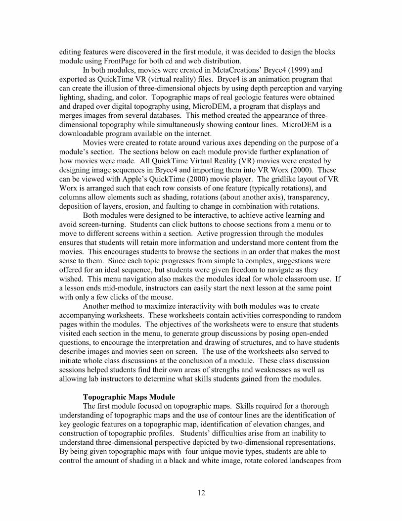
a top view to a side view, raise and lower water levels, and slice into terrains to understand how contour lines and intervals represent elevation changes. Figure M1 shows a simple hill landscape represented by each mode. This module was designed to cover three simple landscapes (hill, valley, and cliff) commonly encountered when reading and interpreting these maps. These three landscapes were presented with the four movie types mentioned above to encourage the visualization of simple features in three dimensions. Movies were created to show the three-dimensionality of landscapes. The shading movies, both black and white and colored, were given the appearance of shadows by using the sun option in Bryce4 (see Figures M1b and M1d). Students could directly compare a flat, two-dimensional map with a three-dimensional map to draw a parallel between specific points and features on the two maps. The ability to see valleys and peaks in terms of shade and light allows to students to discover the relationship between shapes of contour lines and the geologic features they represent.

Upon entering the module, the terms topography and topographic maps are defined. Navigation suggestions are also provided. To notify users where they are within the module and to reduce the likelihood of getting lost, a title was added to the bottom of each page. The first four pages of the website serve to introduce users to the types of animations (user-controlled or instant playing and the four types of animation) they will see throughout the module. This module was constructed to be linear in order to group animations. By doing so, students adapted to each type of animation and were familiar with the changes that could be made to each landscape. This also allowed discussion questions to focus on the elements of an animation and enabled students to relate the landscapes to each other.

Figure 1a. Two-dimensional topographic map of a simple hill.

Figure 1b. Shading movie where users click and drag the mouse up and down to increase and decrease the amount of shade.

Most screens in the module are shown in a split-screen mode where the left half

of the screen is a topographic map of the landscape being studied. On the right half, the various movies are presented. Directly above the movies, arrows are shown to direct users how dragging the mouse will alter the image. Figures 1a and 1b appear on one screen together. Both images on these split screens begin in identical orientations and scales so students can compare contour lines. As the user clicks and drags the mouse upward in the movie on the right, the amount of shading increases as the sun angle

14

changes. Students immediately notice the appearance of hills, valleys, or cliffs, as well as high and low elevation points. The next screen shows colored topographic contours in which the movie rotates both vertically (to rotate up to a side view of the landscape as well as increase shading) and horizontally. Figures 1c and 1d

Figure 1c. Two-dimensional topographic map with color-coded elevations.

Figure 1d. Rotating and shading movie. Clicking and dragging the mouse up and down rotates vertically while changing shade. Landscape can be rotated horizontally by dragging sideways.

appear as a pair on screen. Students are then asked open-ended discussion questions that require observation and interpretation. The questions below represent types of questions asked about a still image of each landscape.

• Can you now envision what this terrain looks like, based on the map? • What is the hill's overall shape? • What are some of the finer details of its shape? • Is it the same steepness on all sides? • Is it aligned in some direction?

To check their responses, students are taken to another screen that shows a continuously playing movie that rotates both vertically (90º) and horizontally (360º). This allows students to discuss details in depth and modify any answers that were debated or unresolved. Students are then asked to write, on their worksheet, a clear verbal description for someone who has never seen each feature. They are given suggestions that may help students write their descriptions. More questions are then provided to help students clarify their descriptions. Finally, a sample description is provided by a field geologist.

The next mode of display for visualizing three dimensional features is the use of flooding water in a terrain (see Figure M1e). By clicking and dragging in the movie,

15

Figure 1e. Flooding movie. Users change the water level by clicking and dragging up and down.

Figure 1f. Slicing terrains movie. Users change the depth of cut by clicking and dragging up and down.

users see how water rises to a level parallel to contour lines. The purpose of this mode is to clarify that contour lines represent a single elevation. Seeing the interaction of water and terrains helps students visualize basic features within an overall landscape. This interactive section allows students to set the water level at a contour line that might have previously been confusing for them. For example, not understanding how contour lines close together can represent a cliff often becomes clear when students altered the water level themselves. After students interact with each feature, they are again asked to clearly describe how the water flooded the area with the three questions below:

• Where does it flood first? Where does it flood last? • What pattern does the water make when it is half way up the slopes?

After interacting with several flooding movies, groups are asked to verbally describe how the land would flood over time, and a sample description is given for the hill and valley but not the cliff. All of the screens up to this point represent the learning cycle exploration phase of the module. The last screen of this section defines contour lines and index contours. This represents the term introduction phase of the learning cycle.

The last mode of visualization consists of creating landscape profiles as slices are made in a terrain. Students actively change the profile by clicking and dragging up and down to slice into or build up, respectively, the terrain (see Figure 1f). The application phase of the learning cycle is then provided by showing a two-dimensional representation of a landscape with a red line drawn on it. Students are given the scenario that they want to hike along the line and shown an elevation profile that corresponds to that path. Then students are taken to several screens where they are asked to predict what the elevation profile for a different path in each of the three features would look like. Figure 2 shows several such screens. As they move to each new question, a different type of movie (increasing shading, rotating colored topographic maps, or slicing into terrains) is provided to help students determine the correct profile.

16

Figure 2. In the application phase of the learning cycle, students are asked to predict what profiles across the three featured landscapes would look like if they were to hike along indicated paths. Block Diagrams Module The interactive blocks module focused on developing students’ visual penetrative ability. A crucial step in reconstructing geologic histories of an area requires the ability to sequence events from youngest to oldest. This is often done by interpreting the order in which events, such as layer deposition, folding, faulting, and intrusions, occurred. These features are often buried beneath the surface leaving only partial structures on which to base conclusions. The sections incorporated into the blocks module were designed to guide students in the visualization process of uncovering or disembedding underlying features. Techniques used to accomplish this included the rotation of blocks, making blocks partially transparent, slicing into blocks, offsetting faults, eroding the tops and sides of blocks, depositing layers, and revealing unconformities. Since this module was created entirely in FrontPage for web distribution, the opening screen of the module contains links to instructional information. “List of Files” takes instructors to a list of individual movies used in the entire module. This allows them to access movies without entering the module. The second link, “Main Module Home”, suggests students start here to receive introductory navigation and movie type information similar to the opening screens of the topographic maps module. Students are also informed in this section how the faces of blocks will be labeled (front, back, left, right, top, and bottom). The third link, “Main Module”, takes students to the main menu of the module and lists the five features they can explore throughout the module. The five sections covered in the module are layers, folds, faults, intrusions, and unconformities. The fourth link takes instructors to Word and PDF files of the worksheets that accompany the module. A worksheet was developed for each of the five main sections in the module. See Figure 3 for an example of the worksheet from the layers section. Once students reach the main menu, they can explore each feature in the order they choose. Students are informed that the topics are easiest to cover in the linear order presented in the menu, but if one section has already been covered or is too simplistic, it can easily be skipped. For the creation of this module, blocks were generated in Bryce4 as one row (rotations) or multirow (rotations in combination with other changes) movies.

17

Image sequences were loaded into VR Worx to generate QTVR movies. This format allows students to interact with movies to control the type and speed of changes that occur.

Figure 3. Layers worksheet used in the blocks module. Each block is shown on the worksheet exactly as students needed to draw it (e.g., cut in half or faces covered). Each main menu topic contains its own submenu. For example, clicking on “Layers” takes students to a screen containing buttons to explore horizontal, gentle, moderate, steep, and vertical layers. Some sections begin with a prediction screen. Here, students are asked to predict how the layers continue from visible to hidden faces of the block. The sequence of screens after this include a rotating opaque block followed by a rotating/changing transparency block. The next screen in the section asks students to predict what the interior of the horizontal layer block looks like. Students are shown the block with a “cutting plane” intersecting it. The purpose of a cutting plane is to cut into a block and understand how subsurface features are oriented. In various movies, students can cut left to right, right to left, or top to bottom to fully understand orientations of features inside the blocks. Figure 4 shows examples of blocks from each of these screens for horizontal layers.

Quizzes were inserted at the end of each section so students could immediately test what they had learned. During the course of a single lab meeting, students completed one or two sections of the blocks modules. Testing after each section offered students feedback upon completion of a section and offered teaching assistants the chance to open the next lab discussion with a review of topics covered the previous day. Quizzes were designed to include a variety of questions, including multiple choice, sketches, and prediction, closely aligned to the types of questions asked throughout each section. Where possible, feedback was given for questions and movies were provided to have

18

students verify their own answers. The last question in each quiz asks students to draw a block when given a series of geologic events.

4a. Opaque block with horizontal layers students can rotate.

4b. Same block as 4a that students can rotate and change transparency.

4c. Left cutting plane. Students are instructed to cut into the block from left to right.

4d. Left cutting plane movie. The block has been cut into 2/3 of the way.

4e. Right cutting plane. Students can cut into the movie by clicking and dragging right to left.

4f. Right cutting plane movie. The block has been cut into 1/4 of the way.

4g. Top cutting plane. Students can cut into the block from top to bottom.

4h. Top cutting plane movie. The block has been cut into 1/3 of the way.

Figure 4. Block movies (transparency and cutting) used for the layers section. The same blocks and movies were also used throughout the folds section.

19

The folds section proceeds exactly as the layers section – with the same progression of screens and the same types of movies: rotations, transparency, cutting side to side and top to bottom. The five subsections of folds include horizontal anticline, horizontal syncline, plunging anticline, plunging syncline, and vertical.

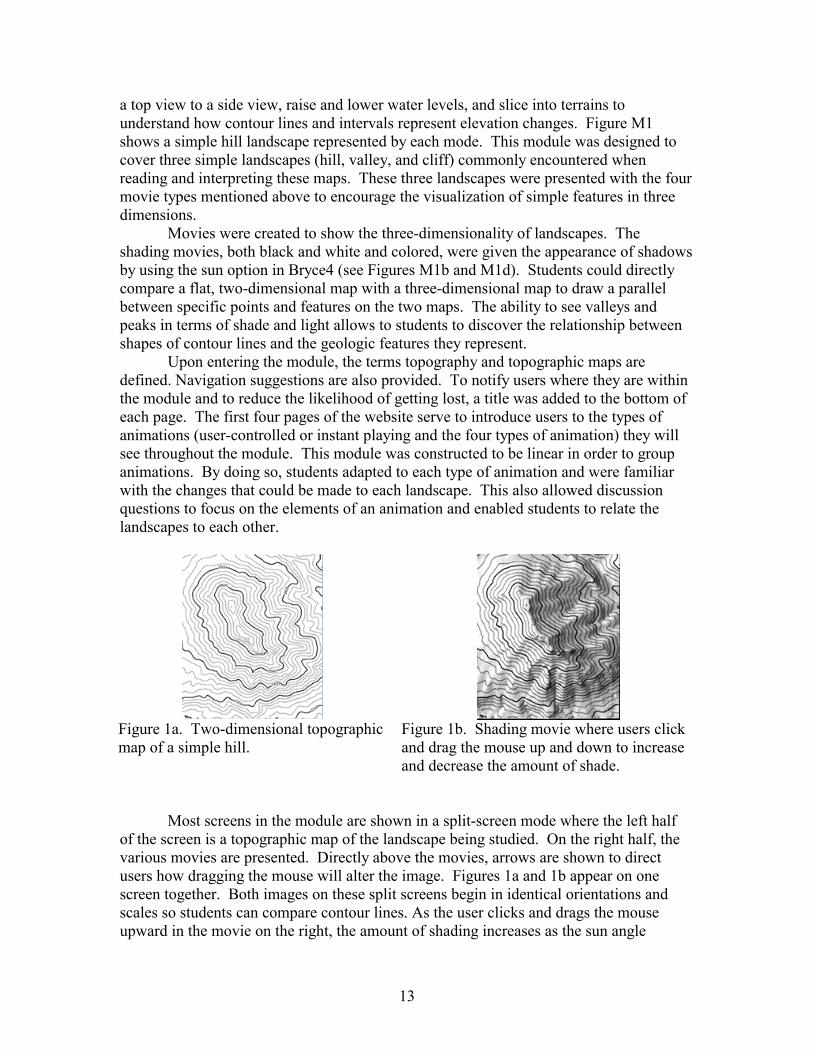
The faults section contains several subsections: types of faults, layers in faults, and folds in faults. With these multiple subsections, clarity of navigation became an issue. In order to minimize student confusion when navigating, several versions of each section were developed. Each version would indicate with yellow text (rather than white) which section or screen was last visited. This helped students monitor their progress and keep track of which sections they completed.

The first subsection of faults, types of faults, covered images and movies of dip-slip, strike-slip, and oblique-slip faults. Students were first given examples of the types of movies they would encounter in this section and then taken to a menu to choose what type of fault they wanted to explore. Movie types in the faults section include rotating, changing transparency, offsetting faults, and eroding surfaces in various combinations. Figure 5 shows movies before and after these changes for plunging syncline folds with strike-slip faults.

5a. Original image of opaque block with horizontal syncline folds in faults section.

5b. Same block as 5a now offset by a strike-slip fault.

5c. Same block as 5b now made partially transparent.

5d. Same block as 5c now eroded on the front side to make that face even.

Figure 5. Four blocks showing the progressive types of movies covered in the faults section of the blocks module. These four blocks specifically show horizontal syncline folds offset by a strike-slip fault.

20

The next section of the module covers intrusions. The main types of movies seen here are rotations, changing transparency, and cutting from top to bottom in a block. This section begins with one intrusion type and adds another type to it. Throughout this section, only one block is shown on each screen. First, only a pluton is explored. Dikes are then added to the pluton to show students the relationship between the two. Sills are then added to the pluton and dike block. Figure 6 shows successive images of these movies. The first row shows only the pluton, the second row shows the pluton with a dike, and the third row shows a pluton, dike, and sill. The questions in this section’s quiz were integrative and focused on having students reconstruct geologic histories from series of events. Students were shown rotating blocks and asked to list events in order they must have occurred. The difficulty in this task required students to identify whether faulting occurred before or after an intrusion based on the amount of offset visible on the surface.

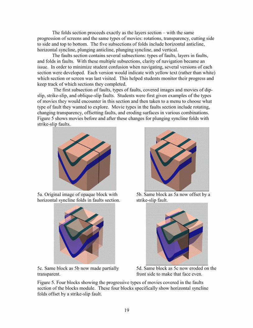
The last section covers unconformities. Students were presented with movies that revealed both horizontal and tilted unconformities. Other features from the module were included in combination with unconformities. For example, a block might contain faulted folds that were eroded and new layers deposited. Students could reveal the unconformities in this section by clicking and dragging the mouse up to examine the intersection of features between erosion and deposition. At the end of this section, and thus the end of the module, an integrated quiz was given. Questions in this quiz ask students to reconstruct a geologic history, predict what an unconformity looks like, sketch a block for a sequence of events, and interpret geologic events from an image taken in the field. Figure 7 shows a series of blocks presented in the integrated quiz section.

21

6a. Opaque block containing pluton. 6b. Partially transparent block cut from

top to reveal pluton.

6c. Partially transparent block of pluton and dike.

6d. Partially transparent block of pluton and dike cut from top to reveal intersection.

6e. Partially transparent block of pluton, dike, and sill.

6f. Partially transparent block of pluton, dike, and sill cut from top to reveal intersection.

Figure 6. Blocks in intrusions section containing progressively more complex subsurface features.

22

7a. Integrative quiz question asking students to place the events (faulting versus intrusion) in the order they must have happened.

7b. Integrative quiz question asking students to place the events (faulting versus intrusion) in the order they must have happened.

7c. Integrative quiz question asking students to place events (tilting of layers, erosion, or unconformity) in the order they must have happened.

7d. Field-related question asking students to identify the key events that occurred to form this feature and the order in which they occurred.

Figure 7. Integrative quiz questions given at the end of the intrusions and unconformities sections.

Computer-Based Tests of Spatial Thinking

Visual-spatial thinking has been recognized as a facet of intelligence that is separate and distinct from verbal ability (Paivio, 1971, 1990; Ekstrom, French, Harmon, & Dermen, 1976; Gardner, 1983). Within the visual-spatial realm, psychometricians have identified a number of factors that contribute to spatial thinking. The Kit of Factor-Referenced Cognitive Tests (Ekstrom, et al., 1976) contains seven paper-based tests that each measure some aspect of spatial thinking. As part of a study investigating spatial thinking in college-level introductory geology class, computer-based versions were developed for two of these tests: the Surface Development Test and the Cubes

23

Comparisons Test (Ekstrom, et al., 1976). The Surface Development Test measures spatial visualization, the ability to manipulate a mental image while the Cubes Comparisons Test measures spatial orientation, the ability to perceive a spatial configuration from alternate perspectives.

Description of Paper Tests In the Surface Development Test, subjects must imagine how a piece of paper can

be folded into some kind of object. They are asked to compare numbered sides of the unfolded object with lettered sides of a folded object to determine which sides are the same. Figure 8 shows a sample item from the test. In Figure 1, the sides indicated by the numbers 2, 3, and 5 respectively correspond with the letters B, G, and H. The Surface Development Test contains six unfolded objects that each have five sides to be identified, resulting in a total of 30 items.

Figure 8. Sample item from the Surface Development Test from the Kit of Factor-Referenced Cognitive Tests (Ekstrom et al., 1976).

In the Cubes Comparisons Test subjects are given two cubes with a different letter, number, or symbol on each of the six faces. They must compare the orientation of the faces on each cube to determine if the two cubes are the same or different. Figure 9 shows a sample item from the test. The two cubes shown are not the same.

Figure 9. Sample item from the Cubes Comparisons Test from the Kit of Factor-Referenced Cognitive Tests (Ekstrom et al., 1976).

24

When the cube on the right is mentally rotated so that the face containing the "A" is in an upright position, then it can be readily seen that the face containing the "X" would now be at the bottom and would not be visible. Because no letter, number, or symbol may be repeated on any of the faces of a given cube, the "X" cannot be both on top and on the bottom of the cube. Therefore, these two cubes must be different. The Cubes Comparisons Test contains 21 pairs of cubes for a total of 21 items. Design Considerations for Computer Tests

Creating computer-based versions of the spatial tests allowed the tests to be modified in ways that were not possible with the paper-based versions. These modifications included:

1) eliminating the verbal cues inherent in the paper tests, 2) providing animated demonstrations as part of the instructions for the tests, and 3) collecting time-to-completion measures on individual items. In the paper version of the Surface Development Test, letters and numbers are

used to identify the sides of the folded and unfolded objects, allowing subjects to indicate their response by recording letters next to numbers. In the computer version of the test, in order to eliminate these verbal cues, the sides of the unfolded objects were color-coded and both the folded and unfolded objects were hot-spot activated. One mouse click is used to select a side of the unfolded object and another is used to indicate its corresponding side. To visually show the response that has been chosen, a miniature folded object with the selected side highlighted, appears onscreen. In Figure 10, the blue side of the unfolded object has been chosen to correspond with the lower right edge of the folded object. This choice is displayed as a small diagram within the color-coded section of the answer box. In a similar manner, the brown side of the unfolded object has been chosen to correspond with the upper left edge of the folded object. As with the paper version, the computer-based version of the Surface Development Test has six unfolded objects that each have five sides to be identified, resulting in a total of 30 items.

Figure 10. Sample item from a computer-based version of the Surface Development Test.

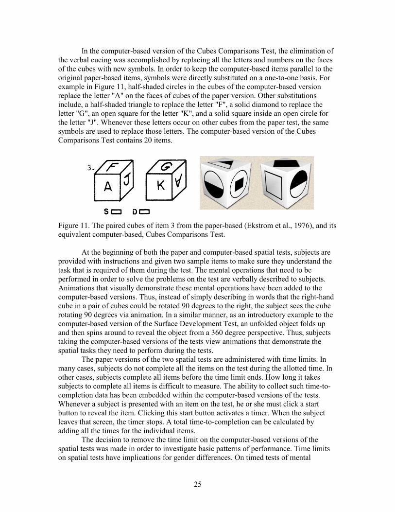
25

In the computer-based version of the Cubes Comparisons Test, the elimination of the verbal cueing was accomplished by replacing all the letters and numbers on the faces of the cubes with new symbols. In order to keep the computer-based items parallel to the original paper-based items, symbols were directly substituted on a one-to-one basis. For example in Figure 11, half-shaded circles in the cubes of the computer-based version replace the letter "A" on the faces of cubes of the paper version. Other substitutions include, a half-shaded triangle to replace the letter "F", a solid diamond to replace the letter "G", an open square for the letter "K", and a solid square inside an open circle for the letter "J". Whenever these letters occur on other cubes from the paper test, the same symbols are used to replace those letters. The computer-based version of the Cubes Comparisons Test contains 20 items.

Figure 11. The paired cubes of item 3 from the paper-based (Ekstrom et al., 1976), and its equivalent computer-based, Cubes Comparisons Test. At the beginning of both the paper and computer-based spatial tests, subjects are provided with instructions and given two sample items to make sure they understand the task that is required of them during the test. The mental operations that need to be performed in order to solve the problems on the test are verbally described to subjects. Animations that visually demonstrate these mental operations have been added to the computer-based versions. Thus, instead of simply describing in words that the right-hand cube in a pair of cubes could be rotated 90 degrees to the right, the subject sees the cube rotating 90 degrees via animation. In a similar manner, as an introductory example to the computer-based version of the Surface Development Test, an unfolded object folds up and then spins around to reveal the object from a 360 degree perspective. Thus, subjects taking the computer-based versions of the tests view animations that demonstrate the spatial tasks they need to perform during the tests.

The paper versions of the two spatial tests are administered with time limits. In many cases, subjects do not complete all the items on the test during the allotted time. In other cases, subjects complete all items before the time limit ends. How long it takes subjects to complete all items is difficult to measure. The ability to collect such time-to-completion data has been embedded within the computer-based versions of the tests. Whenever a subject is presented with an item on the test, he or she must click a start button to reveal the item. Clicking this start button activates a timer. When the subject leaves that screen, the timer stops. A total time-to-completion can be calculated by adding all the times for the individual items.

The decision to remove the time limit on the computer-based versions of the spatial tests was made in order to investigate basic patterns of performance. Time limits on spatial tests have implications for gender differences. On timed tests of mental

26

rotation, male scores are consistently and significantly higher than that of females (Kimura, 1983; Linn and Peterson, 1985; Voyer, Voyer, & Bryden, 1995; Dabbs, Chang, Strong, Milun, 1998). However, there is some evidence to suggest that time, rather than ability per se, may be the differentiating factor in spatial tasks that involve mental rotations (Kail, Carter, & Pellegrino, 1979; Linn & Peterson, 1985).

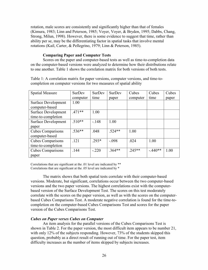
Comparing Paper and Computer Tests Scores on the paper and computer-based tests as well as time-to-completion data

on the computer-based versions were analyzed to determine how their distributions relate to one another. Table 1 shows the correlation matrix for both versions of both tests. Table 1: A correlation matrix for paper versions, computer versions, and time-to-completion on computer versions for two measures of spatial ability Spatial Measure

SurDev computer

SurDev time

SurDev paper

Cubes computer

Cubes time

Cubespaper

Surface Development computer-based

1.00

Surface Development time-to-completion

.471** 1.00

Surface Development paper

.510** -.148 1.00

Cubes Comparisons computer-based

.536** .048 .524** 1.00

Cubes Comparisons time-to-completion

.121 .293* -.098 .024 1.00

Cubes Comparisons paper

.144 -.220 .364** .245** -.440** 1.00

Correlations that are significant at the .01 level are indicated by ** Correlations that are significant at the .05 level are indicated by *

The matrix shows that both spatial tests correlate with their computer-based versions. Moderate, but significant, correlations occur between the two computer-based versions and the two paper versions. The highest correlations exist with the computer-based version of the Surface Development Test. The scores on this test moderately correlate with the scores on the paper version, as well as with the scores on the computer-based Cubes Comparisons Test. A moderate negative correlation is found for the time-to-completion on the computer-based Cubes Comparisons Test and scores for the paper version of the Cubes Comparisons Test. Cubes on Paper verses Cubes on Computer

An item analysis for the parallel versions of the Cubes Comparisons Test is shown in Table 2. For the paper version, the most difficult item appears to be number 21, with only 12% of the subjects responding. However, 73% of the students skipped this question, probably as a direct result of running out of time. For the paper test, item difficulty increases as the number of items skipped by subjects increases.

27

Table 2. Test statistics for the Paper and Computer versions of the Cubes Comparisons Test

Paper-based Cubes Test Computer-based Cubes Test

Item

Num

ber

C

I

S

Mean (N = 146) R

elia

bilit

y C

I

S

Mean (N = 147) R

elia

bilit

y Average Time (sec) R

elia

bilit

y

1 119 25 3 .8082 .7967 122 25 0 .8299 .5124 9.57 .8977 2 126 19 2 .8562 .7897 129 18 0 .8776 .5276 8.28 .8993 3 107 34 6 .7329 .7928 70 70 0 .4762 .5614 12.81 .8931 4 86 55 6 .5822 .7932 114 32 1 .7755 .5017 13.03 .8970 5 105 35 7 .7192 .7840 116 31 0 .7891 .4858 8.63 .8948 6 100 38 9 .6781 .7878 95 50 2 .6463 .5105 13.84 .8934 7 119 22 6 .8082 .7833 120 25 2 .8163 .4956 9.35 .8949 8 102 36 9 .6918 .7825 136 11 0 .9252 .5054 7.61 .8952 9 98 35 14 .6644 .7815 115 32 0 .7823 .5115 13.7 .8944

10 119 8 20 .8082 .7720 112 35 0 .7619 .5104 12.0 .8940 11 91 24 32 .6164 .7694 137 9 1 .9320 .5178 11.7 .8976 12 54 47 46 .3699 .7751 87 60 0 .5918 .5370 12.47 .8914 13 36 51 60 .2466 .7756 80 66 1 .5442 .5063 11.64 .8937 14 74 14 59 .5068 .7624 132 15 0 .8980 .5154 8.82 .8950 15 43 34 70 .2945 .7687 119 28 0 .8095 .4840 8.25 .8940 16 52 10 85 .3493 .7566 120 25 2 .8163 .4889 9.95 .8943 17 52 7 88 .3493 .7636 112 34 1 .7619 .5040 8.89 .8951 18 52 1 94 .3562 .7636 84 63 0 .5714 .6123 11.17 .8954 19 37 12 98 .2534 .7695 129 17 1 .8776 .5241 10.69 .8971 20 40 6 101 .2671 .7688 138 8 1 .9388 .5144 8.02 .8996 21 18 21 108 .1233 .7783

C refers to the number of students selecting the correct response. I refers to the number of students selecting an incorrect response. S refers to the number of students skipping an item. The mean score reflects the difficulty level of an item.

The easiest item on the computer-based version was item 20. Whether the cubes are the same or different can be determined by using visual inspection, instead of rotation. Appendix A contains screen shots of each of the cube pairs created for the computer-based version. One of the least difficult items on both tests was item two, which also only requires visual inspection to solve. The most difficult item on the computer-based version was item 13. To solve this problem, one of the cubes must be rotated twice: 90 degrees on the x-axis and 90 degrees on the y-axis. Alternatively, a 180-degree flip along the z-axis also brings a cube into the necessary comparative position. Overall, the difficulty levels on items on both tests are very similar for the first half of the test. The difficulty levels diverge when subjects begin to run out of time to complete the paper-based version. Surface Development on Paper verses Surface Development on Computer

The items on the Surface Development Test were not constructed in the same parallel fashion as with the Cubes Comparisons Test; therefore comparisons across items on the two tests cannot be made. Unlike with the paper-based Cubes Comparison Test,

28

there is no general increase in difficulty as the paper-based Surface Development test progresses. In other words, difficult items are scattered throughout the test. Table 3. Test statistics for the Paper-based Surface Development Test

Paper-based Surface Development Test

Item

Number Mean (N = 155 )

Reliability

1 .6968 .9133 2 .8194 .9141 3 .5935 .9127 4 .8129 .9154 5 .6323 .9142 6 .7484 .9132 7 .5355 .9133 8 .5419 .9135 9 .7742 .9136

10 .5935 .9137 11 .8452 .9156 12 .8387 .9146 13 .4839 .9124 14 .3161 .9140 15 .7097 .9165 16 .6323 .9119 17 .5355 .9154 18 .4581 .9154 19 .2516 .9176 20 .5032 .9102 21 .1355 .9152 22 .3097 .9118 23 .3677 .9121 24 .4129 .9130 25 .3677 .9109 26 .3419 .9138 27 .4065 .9115 28 .3935 .9112 29 .4000 .9113 30 .4194 .9106

The mean score reflects the difficulty level of an item.

29

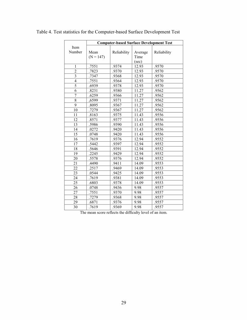
Table 4. Test statistics for the Computer-based Surface Development Test

Computer-based Surface Development Test Item

Number Mean (N = 147)

Reliability

Average Time (sec)

Reliability

1 .7551 .9374 12.93 .9570 2 .7823 .9370 12.93 .9570 3 .7347 .9368 12.93 .9570 4 .7551 .9364 12.93 .9570 5 .6939 .9378 12.93 .9570 6 .8231 .9380 11.27 .9562 7 .6259 .9366 11.27 .9562 8 ,6599 .9371 11.27 .9562 9 .8095 .9367 11.27 .9562

10 .7279 .9367 11.27 .9562 11 .8163 .9375 11.43 .9556 12 .8571 .9377 11.43 .9556 13 .5986 .9390 11.43 .9556 14 .0272 .9420 11.43 .9556 15 .0748 .9420 11.43 .9556 16 .7619 .9376 12.94 .9552 17 .5442 .9397 12.94 .9552 18 .5646 .9391 12.94 .9552 19 .2245 .9429 12.94 .9552 20 .5578 .9376 12.94 .9552 21 .4490 .9411 14.09 .9553 22 .2517 .9469 14.09 .9553 23 .0544 .9425 14.09 .9553 24 .7619 .9381 14.09 .9553 25 .6803 .9378 14.09 .9553 26 .0748 .9436 9.98 .9557 27 .7551 .9370 9.98 .9557 28 .7279 .9368 9.98 .9557 29 .6871 .9376 9.98 .9557 30 .7619 .9369 9.98 .9557

The mean score reflects the difficulty level of an item.

30

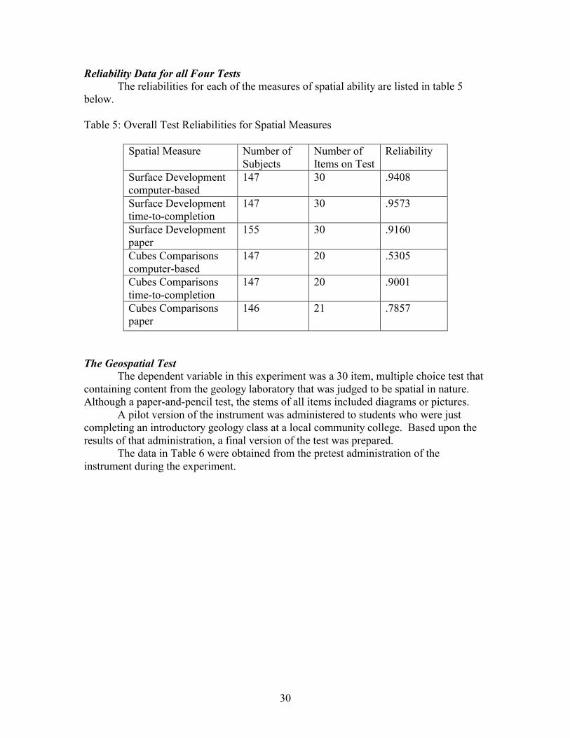
Reliability Data for all Four Tests The reliabilities for each of the measures of spatial ability are listed in table 5

below.

Table 5: Overall Test Reliabilities for Spatial Measures

Spatial Measure

Number of Subjects

Number of Items on Test

Reliability

Surface Development computer-based

147 30 .9408

Surface Development time-to-completion

147 30 .9573

Surface Development paper

155 30 .9160

Cubes Comparisons computer-based

147 20 .5305

Cubes Comparisons time-to-completion

147 20 .9001

Cubes Comparisons paper

146 21 .7857

The Geospatial Test The dependent variable in this experiment was a 30 item, multiple choice test that containing content from the geology laboratory that was judged to be spatial in nature. Although a paper-and-pencil test, the stems of all items included diagrams or pictures. A pilot version of the instrument was administered to students who were just completing an introductory geology class at a local community college. Based upon the results of that administration, a final version of the test was prepared. The data in Table 6 were obtained from the pretest administration of the instrument during the experiment.

31

Table 6. Item analysis and content of Geospatial Test

ITEM Difficulty DiscriminationIndex

Content

1 0.495 0.1 Finding point on map. 2 0.693 0.4 Finding point on map. 3 0.485 0.2 Finding point on map. 4 0.703 0.4 Finding point on map. 5 0.653 0.3 Identifying perspective. 6 0.525 0.4 Identifying perspective. 7 0.733 0.1 Identifying perspective. 8 0.733 0.6 Cross-section. 9 0.465 0.6 Cross-section. 10 0.594 0.6 Cross-section. 11 0.594 0.4 Sequence of events. 12 0.782 0.4 Sequence of events. 13 0.762 0.4 Sequence of events. 14 0.673 0.4 Sequence of events. 15 0.277 0.4 Sequence of events. 16 0.535 0.5 Sequence of events. 17 0.515 0.7 Sequence of events. 18 0.822 0.4 Block diagram. 19 0.713 0.5 Block diagram. 20 0.822 0.2 Block diagram. 21 0.584 0.7 Block diagram. 22 0.723 0.4 Block diagram. 23 0.653 0.6 Map problem. 24 0.733 0.6 Map problem. 25 0.594 0.3 Map problem. 26 0.723 0.6 Map problem. 27 0.347 0.3 Map problem. 28 0.307 0.2 Map problem. 29 0.762 0.3 Map problem. 30 0.762 0.6 Topographic profile

The K-R 20 reliability for the entire Geospatial Test was 0.75 on the pre-test and 0.78 on the post-test.

THE EXPERIMENT

Design of the Project

The project was to create and evaluate a group of computer-based modules for college-level instruction in geology. These were appropriate for use in introductory laboratories as well as upper division courses for geology majors. The materials focused on exposing “The Hidden Earth,” presenting problems involving the surface expression

32

of structural features and the shallow structure of the earth’s interior. The modules were situated in complex, real-life problems and activities that are characteristic of the practice of geology, and its associated reasoning (Frodeman, 1995; Ault, 1998; Drummond, 1999). Computer-based materials were built with the program Bryce3D. This program allows the creation of detailed and realistic, two-dimensional representations depicting three-dimensional perspectives of simple and complex geologic structures and landscapes. The 3D models can be rotated, sectioned, disassembled, or successively unburied. A series of images can be used to depict sequential geologic histories, such as deposition of successive layers, followed by erosion into realistic-looking landscapes. This approach is an analog of strategies that have been shown in previous research to be effective in the development of spatial reasoning. This project sought to embed spatial learning in the context of real-life, complex problems that are authentic. They were taken from among actual problems that geologists deal with in everyday life. The expectation was that this would increase the development of spatial ability and improve the transfer to relevant problem solving. This hypothesis was to be tested in a quasi-experimental design in which control and experimental groups are administered a content assessment and two spatial/visual measures as pre- and post-tests. The Context The experiment was conducted during the first Arizona State University summer session, beginning on Tuesday, May 29 and ending on Friday, June 29, 2001. This consisted of 5 weeks of classes, meeting 1 ½ hours per day. Two sections met from approximately 7-9 a.m. and two from 11 a.m.-1 p.m. Subjects were students in Geology 103, a one credit-hour introductory geology laboratory. Although Geology 103 is associated with the lecture course Geology 101, “Introduction to Geology,” concurrent enrollment is not required, and the content of the lecture and the laboratory are not coordinated. The laboratory course enrolled approximately 100 students divided among four sections. Four sections of Geology 103 were taught, each by a different graduate teaching assistant. Two sections each were assigned to either the control or experimental condition. To eliminate time-of-day effects, a control and experimental group were assigned to each starting time. Teaching assistants were fully briefed on the nature of the experiment, and members of the research team met with them weekly to discuss the nature of the experimental and control conditions. Members of the research team also observed both control and experimental classes on a regular basis to ensure that the experimental conditions are being met. Both control and experimental classes studied from a laboratory manual written by Stephen J. Reynolds, Julia K. Johnson and Edmund Stump, titled “Observing and Interpreting Geology (2001).” This manual covers the traditional content of an introductory geology laboratory in an unconventional manner. The first seven chapters are anchored in a series of computer simulations created in a virtual environment called “Painted Canyon.” In these chapters, students are introduced to topographic maps, minerals and rocks, geologic maps and geologic history, and environmental issues. Chapters 8 through 11 are devoted to the geology of selected regions of Arizona, and lead

33

to a field trip at a location near the University. The final three chapters engage students in a study of the geology of their own home town, the exploration of a geological setting in a virtual environment, an evaluation of the economic potential of selected mineralized areas, and the fossils of the Colorado Plateau.

Two unique computer-based measures of spatial orientation and spatial visualization were created for this study. These were created by this research group as modifications of instruments contained within the “Kit of Factor-Referenced Cognitive Tests” by Ekstrom, et al. (1976). The dependent variable was a geospatial assessment based upon the content of the laboratory manual.

The geospatial assessment was administered as a paper-and-pencil test to all students in all sections on the first and the last days of the first summer session. They were told that their grade would depend in part on their performance on the second content assessment. The two computer-based spatial measures were administered to all students during the first and last weeks of the first summer session. Subjects were removed in groups of ten to an adjacent laboratory for computer-based testing. It required less than two days to complete this phase of the assessment.

The experiment was a quasi-experimental pre-test/post-test design with control and experimental groups. Analysis of Variance was used to test the hypotheses that there are no initial differences among experimental and control groups on any pre-test measure, and that the experimental groups perform at a significantly higher level than the control groups on all post-test measures. Step-wise multiple regression analysis was used to estimate the amount of variance in achievement that is shared with spatial measures.

RESULTS

Sample Distribution The sample consisted of 103 subjects, of whom 48 were male and 55 were female. The groups were unequal in size, with 44 subjects in the control group and 59 in the experimental group. Although subjects self-selected into individual sections of the course, the distribution of by gender across the sections was not random (Table 7). Males exceeded females in the control group by a factor of 1.4/1 and females exceeded males in the experimental group by a factor of 1.7/1. Table 7. Distribution of Subjects by Gender and Group

Group Male Female Total Control 26 18 44 Experimental 22 37 59 Total 48 55 103

This unusual sample bias is a classic example of the difficulties of quasi-

experimental design with intact groups. The normal assumption of a quasi-experimental design of the sort used in this study is that the comparison groups will be equivalent. This has not turned out to be the case in this instance. As will be shown in the analyses that follow, initial mean scores on many variables were lower for females than for males.

34

This has led to a set of results in which initial mean scores of the experimental group tend to be significantly lower than those of the control group.

Attrition rates were relatively high. Only 89 students took both the pretest and the final examination for the course. In addition, many students failed to complete one or more of the spatial measures. The number of students completing each measure will be indicated in the analyses that follow. The Geospatial Test The effects of the experiment are analyzed through the application of a three-way Analysis of Variance. In this analysis, the dependent variable is performance on the Geospatial Test. SCORE reflects differences in performance from pretest to posttest, and is treated here as a repeated measure. CONDITION refers to control vs. experimental group, and GENDER to males vs. females. The results are shown in Table 8. Table 8. Three-way Analysis of Variance (SCORExCONDITIONxGENDER) of Scores on Geospatial Test

F df p SCORE 161.266 1, 85 0.00* SCORExCONDITION 3.844 1, 85 0.05* SCORExGENDER 4.853 1, 85 0.03* SCORExCONDITIONxGENDER 0.213 1, 85 0.65

There was a significant main effect for SCORE, with higher posttest than pretest scores for the entire sample. There were significant two-way interactions between SCORE and CONDITION, and between SCORE and GENDER. There was no significant three-way interaction.

In order to assess the magnitude of the experimental effect, normalized gain scores were computed for each student. Often referred to in the Physics Education literature as “Hake Scores,” these reflect the increase from pretest to posttest score as a percentage of the total possible increase (normalized gain = posttest-pretest/total possible-pretest). The results are displayed as histograms in Figure 12.

C o n t r o l G r o u p

1 .0 0

.7 5

.5 0

.2 5

0 .0 0

- .2 5

- .5 0

- .7 5

- 1 .0 0

- 1 .2 5

2 0

1 0

0

S td . D e v = .4 3

M e a n = .4 5

N = 4 4 .0 0

E xp e r im e n t a l G r o u p

1 .0 0

.7 5

.5 0

.2 5

0 .0 0

- .2 5

- .5 0

- .7 5

- 1 .0 0

- 1 .2 5

1 6

1 4

1 2

1 0

8

6

4

2

0

S td . D e v = .3 0

M e a n = .6 0

N = 4 7 .0 0

Figure 12. Normalized Gain Scores of Experimental and Control Groups on the Geospatial Test.

35

The mean control group gain scores were 0.45 (45%), and the distribution remained normally distributed. In contrast, mean experimental group gain scores were 0.60 (60%) and badly skewed as a result of a ceiling effect. A large number of students in the experimental group achieved gains in the upper ranges, 75% and above. If the Geospatial Test had been somewhat more difficult, it is likely that the distribution of experimental group scores would also have been normal, and the differences between the means even greater. Pretest mean scores of the control group were lower than those of the experimental group, whereas posttest mean scores were approximately equal. This undoubtedly resulted from the unequal distributions of males and females in the control and experimental groups and differences in their performance on the Geospatial Test. The experimental treatment thus had the effect of equalizing previously unequal scores between the control and experimental groups, and demonstrating the effectiveness of the experimental materials. It also had the effect of equalizing initial differences in performance between males and females. Normalized gain scores for the entire sample are displayed separately by gender in Figure 13. They are considerably larger for females (56%) than for males (48%). While there is a slight ceiling effect for females, it is not as dramatic as the earlier example.

Ma le

1 .00.75

.50.25

0 .00-.25

- .50-.75

-1 .00-1.25

14

12

10

8

6

4

2

0

Std . Dev = .38 Mean = .48

N = 36 .00

F e m a le

1 .00.75

.50.25

0 .00-.25

- .50-.75

-1 .00-1.25

20

10

0

Std . Dev = .37 Mean = .56

N = 55 .00

Figure 13. Normalized Gain Scores of Males and Females on the Geospatial Test. Descriptive statistics for the sample of 89 students who took the Geospatial Test as both a pre-test and post-test are given in Table 9. These permit a more detailed comparison of male and female performances in the control and experimental groups. Figure 14 demonstrates the importance of gender as a variable in performance on the Geospatial Test. Females in both the control and the experimental groups experienced greater growth in their Geospatial Test scores from pretest to posttest than did males. Although the effect was smaller, both males and females in the experimental group showed greater improvement than those in the control group. These results are exactly what were expected from the observation of a CONDITION x GENDER interaction.

36

Table 9. Descriptive Statistics for Sample Performance on Geospatial Test

PREGEOSPATIAL MEAN S.D. n Control Male 21.67 4.50 24 Female 18.61 5.01 18 Total 20.36 4.91 42 Experimental Male 20.67 3.45 12 Female 16.63 4.73 35 Total 17.66 4.75 47 Entire Sample Male 21.33 4.15 36 Female 17.30 4.87 53 Total 18.93 4.99 89 POSTGEOSPATIAL Control Male 25.79 3.05 24 Female 24.33 5.04 18 Total 25.17 4.04 42 Experimental Male 26.17 3.43 12 Female 24.57 3.88 35 Total 24.98 3.80 47 Entire Sample Male 25.92 3.14 36 Female 24.49 4.26 53 Total 25.07 3.89 89

0

5

10

15

20

25

30

control females experimentalfemales

control males experimentalmales

Figure 14. Pretest (left) and Posttest (right) Means of Males and Females in Experimental and Control Groups on the Geospatial Test.

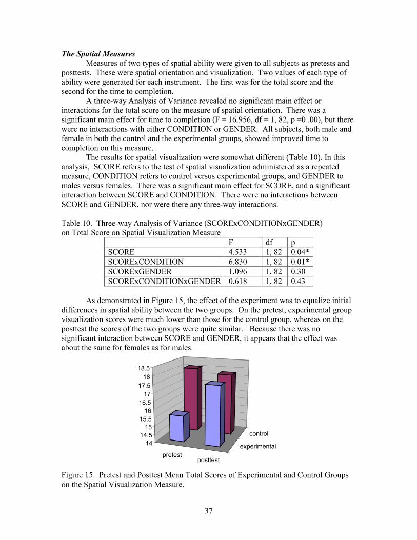
37

The Spatial Measures Measures of two types of spatial ability were given to all subjects as pretests and posttests. These were spatial orientation and visualization. Two values of each type of ability were generated for each instrument. The first was for the total score and the second for the time to completion.

A three-way Analysis of Variance revealed no significant main effect or interactions for the total score on the measure of spatial orientation. There was a significant main effect for time to completion (F = 16.956, df = 1, 82, p =0 .00), but there were no interactions with either CONDITION or GENDER. All subjects, both male and female in both the control and the experimental groups, showed improved time to completion on this measure.

The results for spatial visualization were somewhat different (Table 10). In this analysis, SCORE refers to the test of spatial visualization administered as a repeated measure, CONDITION refers to control versus experimental groups, and GENDER to males versus females. There was a significant main effect for SCORE, and a significant interaction between SCORE and CONDITION. There were no interactions between SCORE and GENDER, nor were there any three-way interactions. Table 10. Three-way Analysis of Variance (SCORExCONDITIONxGENDER) on Total Score on Spatial Visualization Measure

F df p SCORE 4.533 1, 82 0.04* SCORExCONDITION 6.830 1, 82 0.01* SCORExGENDER 1.096 1, 82 0.30 SCORExCONDITIONxGENDER 0.618 1, 82 0.43

As demonstrated in Figure 15, the effect of the experiment was to equalize initial differences in spatial ability between the two groups. On the pretest, experimental group visualization scores were much lower than those for the control group, whereas on the posttest the scores of the two groups were quite similar. Because there was no significant interaction between SCORE and GENDER, it appears that the effect was about the same for females as for males.

pretestposttest

experimental

control14

14.515

15.516

16.517

17.518

18.5

Figure 15. Pretest and Posttest Mean Total Scores of Experimental and Control Groups on the Spatial Visualization Measure.

38

This was not the case for time to completion on the test of spatial visualization Table 11). In this instance, there was a significant main effect for time to completion, with students completing the posttest more quickly than the pretest, and a significant interaction between SCORE and GENDER. There was no significant interaction between SCORE and CONDITION nor was there a significant three-way interaction. Table 11. Three-way Analysis of Variance (SCORExCONDITIONxGENDER) for Time to Completion on Spatial Visualization Measure

F df p SCORE 75.899 1, 82 0.00* SCORExCONDITION 2.199 1, 82 0.14 SCORExGENDER 5.683 1,82 0.02* SCORExCONDITIONxGENDER .115 1, 82 0.74

Figure 16 shows the effects of gender on time to completion. In this case, males

began the experiment with somewhat longer times to completion than females, and the two groups were about the same at the end.

pretestposttest

female

male0

20

40

60

80

100

120

femalemale

Figure 16. Pretest and Posttest Mean Times to Completion of Females and Males on Spatial Visualization Measure. Spatial Ability and Achievement The matrix of correlations between measures of spatial and geospatial ability is presented in Table 12. There are no significant correlations among measures of time to completion of spatial orientation or visualization. Because of this, time was eliminated as a variable in further analyses. However, the correlations between total scores on the spatial and geospatial measures are quite high, ranging from a low of 0.39 to a high of 0.57. This reflects shared variances (r-square) averaging 19% for spatial orientation and 29% for spatial visualization between the spatial and geospatial measures.

39

Table 12. Coefficients of Correlation Among all Variables 1 2 3 4 5 6 7 8 9

1 PreOrientation -score

1.00

2 PostOrientation -score

0.72* 1.00

3 PreOrientation -time

-0.02 -0.06 1.00

4 PostOrientation -time

-0.10 -0.01 0.81* 1.00

5 PreVisualization -score

0.62* 0.59* 0.01 -0.05 1.00

6 PostVisualization -score

0.59* 0.55* 0.11 0.09 0.84* 1.00

7 PreVisualization -time

0.04 -0.01 0.45* 0.36* -.20 0.31* 1.00

8 PostVisualization -time

-0.10 -0.08 0.39* 0.47* -0.03 0.15 0.64* 1.00

9 PreGeospatial -score

0.46* 0.42* -0.03 -0.16 0.57* 0.49* 0.00 -0.21 1.00

10

PostGeospatial -score

0.39* 0.48* 0.15 0.07 0.55* 0.55* 0.03 -0.06 0.57*

*p = 0.05 Because students entered the course with a good deal of prior geospatial knowledge, and because of the correlations between spatial and geospatial ability, it was necessary to estimate the amount of variance in posttest geospatial scores that was shared with spatial scores after the contribution of initial ability had been co-varied. In order to accomplish this, a Stepwise Multiple Regression Analysis, with pretest Geospatial scores entered as a covariate at the first step, was completed (Table 13). Prior knowledge, as Table 13. Regression of Posttest Geospatial Scores Against Pretest Scores of Spatial Orientation and Visualization and of Geospatial Ability B Std. Error Beta t probability (Constant) 16.009 1.992 8.306 0.000 Geospatial .291 0.085 0.373 3.433 0.001 Orientation 4.4E-02 0.162 0.032 0.275 0.784 Visualization 0.173 0.074 0.296 2.339 0.022 measured by the Geospatial Test, and initial ability at spatial visualization achieved significant Betas in this analysis. The Beta for pretest scores on the spatial orientation measure did not reach the level of statistical significance. The variance shared between the posttest geospatial ability and all pretest variables of spatial and geospatial ability was 38.4% (r=.620). The relative influence of the separate factors in the equation can be evaluated by comparing Beta weights, or standard partial regression coefficients, of the independent variables. Such a partial coefficient expresses the change in the dependent variable due to a change in one

40

independent variable with the remaining variables held constant. In any regression, Beta weights are the same regardless of the order in which the variables are entered.

Both prior knowledge and visualization ability contributed significantly to the equation predicting posttest Geospatial Test scores. Although the Beta for prior knowledge was somewhat higher than the Beta for spatial visualization, the two are similar enough to state that as a first order approximation the two contribute equally to the regression equation. Summary

Although all subjects profited from both the control and the experimental conditions, the effectiveness of the treatment experienced by the experimental group has been confirmed. Using both Analysis of Variance and a comparison of normalized gain scores, it has been demonstrated that students in the experimental group profited more than those in the control group. Very powerful gender effects have also been demonstrated. The experiment had the result of equalizing the performance of males and females in a case where the performance of males was initially superior to that of females. Again, although females profited from both treatments, it appears that the experimental condition was slightly preferable. There was little effect on the abilities of students in spatial orientation as a result of either condition, nor did this variable affect achievement. This was not, however, the case for spatial visualization. The experimental treatment was very effective at improving scores and lowering times to completion. In this instance, the performance of males appears to have been differentially improved over that of females. A regression of performance on the posttest Geospatial Ability measure against pretest variables showed that the normalized regression coefficients for prior knowledge and visualization ability were quite similar.

DISCUSSION

Reform of science education must be predicated on research on learning and teaching materials and practices that are developed from that research.

Geoscience Education Working Group (1997)

This project demonstrates that spatial ability can be improved through

instruction, leading to improved learning, and that differences in performance between the genders can be eliminated with such an intervention. This result was reached through the creation and application of a set of innovative, computer based materials that can be widely used in introductory laboratory courses at colleges and universities. But more important, this study provides evidence from a naturalistic setting that demonstrates the effectiveness of those materials.

Spatial orientation and visualization are commonly understood as factorially distinct mental abilities. In this study, participants improved in visualization, but not in spatial orientation. In addition, visualization is a significant predictor of the amount learned, but spatial orientation is not. Even more important is the finding that

41

visualization and prior knowledge have approximately equal predictive power in a regression equation against post-test knowledge scores. This may be the strongest demonstration yet of the potency of spatial ability in facilitating learning, and of the importance of being able to visually transform an image to the nature of that learning process.

Because of time limitations and difficulties with preparing computer-based materials, we limited our inquiry to the most obvious and well-known examples of spatial ability. Even then, questions remain about the nature of spatial orientation and visualization, and how these interact with student learning. The observation of significant correlations is interesting, but we must now move forward to an explanation of how students manipulate images and use that information to generate knowledge. We expect that this answer will not be reached through quasi-experimental studies such as this one. In fact, we hope to soon begin a series of studies of a more qualitative nature in which the question of how students use images to negotiate meaning is addressed.

At least two other important spatial factors remain unexamined in our study. The first is the process of “disembedding” or “restructuring,” as defined by measures such as the Embedded Figures Test. We are confident that this is an important variable, and available tests are adequate for an appropriate study. However, we have not yet completely defined how a working geologist would apply this ability to field studies, nor have we been able to create computer-based activities that mimic this process. We intend to create an interactive, computer-based module that involves disembedding figure from ground in realistic geological contexts, and replicating the current study in the near future.

Although we did not examine the variable of visual penetrative ability (VPA) discussed by Kali and Orion (1996), we did observe student behaviors that suggested the operation of such a factor. This was especially true in problems involving block diagrams. When attempting to interpret a block penetrated by an inclined plane, many students seemed unable to see the projection of the plane through the block. When asked to complete a drawing of the intersection of a plane with the block faces, students often continued the line from the known face across the unknown one as though it were a linear rather than a planar element. The line seemed to be perceived as something found only on the outside of the block, that wrapped around the block in a continuous fashion. We also observed many solutions where the line was drawn at an angle someplace between this interpretation and the correct one, as though students had an insight but were drawn perceptually to the incorrect solution. We also observed that this problem generated spirited discussions within groups where the correct and incorrect interpretations were held by members.

This study also has important implications to the issue of factors that influence the success of women in science. Gender differences in both spatial ability and achievement have been found by almost all those who have studied the topic. As suggested in our review of the literature, the question of the origin of these differences has not been answered. In this study, a relatively brief intervention succeeded in eliminating gender differences in spatial ability and closing the performance gap between males and females. This replicates a recent finding, in a study of success in engineering, that “females improved more than males in spatial ability” (Hsi, et al., 1997). Both results speak very strongly in favor of the position that observed gender differences are

42

the result of differences in experience, and not of innate mental abilities, and that they can be eliminated by relatively minor treatments.

Although this intervention was brief, and did not allow an extended qualitative examination of student behaviors, all of the members of the research team spent time in the experimental classroom watching students work and talking to them about what they were doing. One set of observations, to which all observers agree, deserves discussion in this context. It appeared that the dynamics of group interactions depended heavily on the gender mix of the groups. This was especially evident when all-male and all-female groups were compared.

In all-male groups, the interactions were extremely limited. Since only one person could control the computer terminal, that tended to be the individual who already knew the most about the topic and who directed the activities of the group. In fact, in all-male groups, those who were not running the computer were generally uninvolved, sitting quietly and inattentively until an answer was reached that they could record on their work-sheet. There was virtually no discussion among members of the group, except in cases where the dominant male explained the results and answer to others.

All-female groups tended to work in a much different fashion. The person managing the computer was more often directed by the group about what action to take. The origin of this dynamic is not clear. Perhaps it was because no single clear leader in terms of computer skills emerged in female groups, or perhaps it was because females prefer to work in a more collaborative manner. Whatever the reason, female working groups tended to negotiate the action to be taken, and then to discuss the results among themselves before moving on to another action. This applied also to decisions about what information and conclusions to record on their work-sheets. There was a great deal more discussion and negotiation of meaning in groups composed entirely of females.

Much of the research comparing technology-based instruction to other methods has proven to be inconclusive. In general, technology is expensive and difficult to use, and not clearly superior to more traditional methods of instruction. It is our opinion that the superiority of computer-based education only becomes evident in cases where it is not possible to deliver the instruction by any other means.

A case in point is the topographic mapping module in this study. The geology department at this university has been using the “volcano in a box” laboratory, which originated many years ago with the Earth Science Curriculum Project, for some years in its introductory laboratories. However, creation of other landforms for students to explore in the same way has proven difficult. We are able to render virtually any topographic feature in the world into a three-dimensional, manipulable image. In addition, we have been able to create many new ways for students to manipulate these images that are not possible with the physical model.

The same could be said for the geologic blocks module. A teaching laboratory typically has only one or two three-dimensional block diagrams for students to work with. We have been able to produce dozens, with an exceptionally wide variety of features. And we can allow students to do things, like making the blocks transparent, that are impossible to do with physical models.

We also present these modules as a proof-of-concept for the use of computer-based instructional materials in a constructivist context. We allow students to begin their work with a playful, exploratory investigation of a variety of images. They work in

43

groups, interacting with the computer and using worksheets to record their emerging interpretations of what they are seeing. We ask them to create pictures in their mind long before we offer formalisms such as the definition of contour intervals or the names of particular kinds of folds or faults.

One of the characteristics of science curricula since the reform movement of the 1960’s has been their attempt to accurately portray the nature of science. This was commonly expressed as a concern for the structure of the discipline (Bruner, 1960). Initially, this took form as something approximating what is usually described as the “scientific method,” and curricula taught students to observe, infer and test hypotheses. More recently, science educators have recognized significant differences among scientists working under different paradigms, and come to see that there may be many structures of this discipline we call science.

We have been trying to emphasize what we believe is a structure of the discipline of geology that is especially important, and perhaps more so in this case than in other sciences. Geologists use time and space to construct theories about the earth. While the more traditional processes of science remain important, they are to some extent subordinated to the temporal-spatial reasoning that we think is characteristic of geology.

We believe that instruction should be anchored in authentic contexts and faithful to the structure of the geological sciences. Unfortunately, introductory courses at the college and university level are often disconnected collections of topics with no apparent coherence, and the tasks given to students in the laboratory bear little resemblance to the work of practicing scientists. We have tried to create a single unifying structure in which we situate instruction. Painted Canyon, a computer-generated terrain, is the context within which students learn geology in the laboratory. We try to represent the thought process of the geologist through a series of tasks for students that are as similar to those being undertaken by practicing geologists as we can possibly make them. This study challenges conventional methods of teaching science. Rather than working from dull and uninteresting workbooks, students need to be engaged actively in realistic settings that are like those experienced by geologists themselves. Rather than dealing entirely in verbal forms of learning, they should engage all of the mental faculties, including but not limited to spatial visualization.

Finally, engaging in situated activities helps students to develop a set of intellectual skills that are demonstrably important to the learning of science and to the practice of geology. And it gives them some sense of what it is like to be a geologist. That, it seems to us, is among the most important goals of any course in laboratory science.

Acknowledgements: This research has been supported by funds provided through NSF grant EAR-9907733. For Information Contact: � Michael Piburn – mike.piburn@asu.edu � Stephen Reynolds – sreynolds@asu.edu

Most materials are available online at http://reynolds.asu.edu

44

REFERENCES

Albanese, M. & Mitchell, S. (1993). Problem-based learning: A review of

literature on its outcome and implementation issues. Academic Medicine, 68(1), 52-80. Ault, C.R., Jr. (1998). Criteria of excellence for geological inquiry: the necessity

Of ambiguity. Journal of Research in Science Teaching, 35, p. 189-212. Authorware 5 [Computer Software]. (1998). San Francisco, California:

Macromedia, Inc. Brown, J., Collins, A. & Duguid, P. (1989). Situated cognition and the culture of

learning. Educational Researcher, 18(1), 32-41. Bruner, J. (1960). The Process of Education. Cambridge, MA: Harvard University Press. Chapter 2. The Importance of Structure.

Bryce4 [Computer Software]. (1999). Carpinteria, California: MetaCreations Corporation.

Burnett, S. & Lane, D. (1980). Effects of academic instruction on spatial visualization. Intelligence, 4(3), 233-242.

Carter, C., LaRussa, M. & Bodner, G. (1987). A study of two measures of spatial ability as predictors of success in different levels of general chemistry. Journal of Research in Science Teaching, 24(7), 645-657.

The Cognition and Technology Group at Vanderbilt (1990). Anchored instruction and its relation to situated cognition. Educational Researcher, 19(6), 2-10.

Cohen, H. (1983). A comparison of the effect of two types of student behavior with manipulatives on the development of projective spatial structures. Journal of Research in Science Teaching, 20(9), 875-883.

Dabbs, J. M., Chang, E., Strong, R. & Milun, R. (1998). Spatial ability, navigation strategy, and geographic knowledge among men and women. Evolution and Human Behavior, 19, 89-98.

Devon, R., Engel, R. and Turner, G. (1998). The effects of spatial visualization skill training on gender and retention in engineering. Journal of Women and Minorities in Science and Engineering, 4, 371-380.

Drummond, C. (1999). Facilitating scientific thoughtfulness for non-science majors. Journal of Geoscience Education, 47, p. 45-55.

Ekstrom, R., French, J., Harman, H. & Dermen, D. (1976). Manual for Kit of Factor Referenced Cognitive Tests. Princeton, NJ: Educational Testing Service.

Eley, M. (1993). The differential susceptibility of topographic map interpretation to influence from training. Applied Cognitive Psychology, 7(23-42). influence from training.

Ericsson, K. & Smith, J. (1991). Prospects and limits of the empirical study of expertise: An introduction. In Ericsson and Smith (eds.), Toward a General Theory of Expertise: Prospects and Limits. Cambridge: Cambridge University Press.

Frodeman, R.L. (1996). Envisioning the outcrop. Journal of Geoscience Education, 44, p. 417-427.

Frodeman, R.L. (1995). Geological reasoning: geology as an interpretive and Historical science. Geological Society of America Bulletin, 107, p. 960-968.

FrontPage 2000 [Computer Software]. (2000). Microsoft Corporation.

45

Gardner, H. (1985). Frames of Mind: The Theory of Multiple Intelligences. Basic Books.

Hsi, S., Linn, M. & Bell, J. (April, 1997). The role of spatial reasoning in Engineering and the design of spatial instruction. Journal of Engineering Education, 151- 158.

Kail, R., Carter, P., & Pellegrino, J. (1979). The locus of sex differences in spatial ability. Perception and Psychoanalysis, 26, 182-186.

Kali, Y. & Orion, N. (1996). Spatial abilities of high-school students and the perception of geologic structures. Journal of Research in Science Teaching, 33(4), 369- 391.

Kali, Y., & Orion, N. (1997). Software for assisting high-school students in the spatial perception of geological structures. Journal of Geoscience Education, 45, p. 10-21.

Kimura, D. (1992). Sex differences in the brain. Scientific American, 267, 118-125.

Linn, M. and Petersen, A. (1985). Emergence and characterization of sex differences in spatial ability: A meta-analysis. Child Development, 56, 1479-1498.

Lord, T. (1985). Enhancing the visuo-spatial aptitude of students. Journal of Research in Science Teaching, 22(5), 395-405. Lord, T. (1987). A look at spatial abilities in undergraduate women science majors. Journal of Research in Science Teaching, 24(8), 757-767.

Maccoby, E. (1966). Sex differences in intellectual functioning. In Maccoby, E. (Ed.), The Development of Sex Differences. Stanford, CA: Stanford University Press. Pp. 25-55.

Maccoby, E. and Jacklin, C. (1974). The Psychology of Sex Differences. Stanford, CA: Stanford University Press.

Maguire, E., Gadian, D., Johnsrude, I., Good, C., Ashbruner, J., Frackowiak, R. & Frith, C. (2000) Navigation-related structural change in the hippocampi of taxi drivers. PNAS, 97(8), 4398-4403.

McArthur, J. and Wellner, K. (1996). Reexamining spatial ability within a Piagetian framework. Journal of Research in Science Teaching, 33(10), 1065-1082.

McClurg, P. (19 ). Investigating the development of spatial cognition in problem-solving microworlds. Journal of Computing in Childhood Education, 3(2), 111- 126.

Muehlberger, W.L., & Boyer, R.E. (1961). Space relations test as a measure of visualization ability. Journal of Geological Education, 9, p. 62-69.

Paivio, A. (1971). Imagery and verbal processes. New York: Holt Rinehart and Winston.

Paivio, A. (1990). Mental representations: A dual coding approach. New York: Oxford University Press.

Pallrand, G. & Seeber, F. (1984). Spatial ability and achievement in introductory physics. Journal of Research in Science Teaching, 21(5), 507-516.

Piburn, M. (1980). Spatial reasoning as a correlate of formal thought and science achievement for New Zealand students. Journal of Research in Science Teaching, 17(5), 443-448.

Piburn, M. (1992). Meta-analytic and multivariate procedures for the study of attitude and achievement in science. Dortmund, Germany: International Council of

46

Associations for Science Education (ICASE). Rieber, L.P. (1995). A historical review of visualization in human cognition.

Educational Technology Research and Development, 43(1), 45-56. Roe, A. (1961). The psychology of the scientist. Science, 134, 456-59. Rudwick, M.J.S. (1976). The emergence of a visual language for geological

science 1760-1840. History of Science, 14, p. 149-195. Schofield, J. & Kirby, J. (1994). Position location on topographical maps: Effects

of task factors, training, and strategies. Cognition and Instruction, 12(1), 35-60. Shepard, R. (February 1978). The mental image. American Psychologist, 125-

137. Shepard, R. (1988). The Imagination of the scientist. In K. Egan & D. Nadaner

(Eds.), Imagination and education (pp. 153-185). New York: Teachers’ College Press. Shepler, R. & Metzler, J. (1971). Mental rotation of three-dimensional objects.

Science, 171, 701-703. Smith, D. & Hoersch, A. (1995). Problem-based learning in the undergraduate

geology classroom. Journal of Geological Education, 43, 385-390. The VR Worx 2.0 [Computer Software]. (2000). Pittsburgh, Pennsylvania: VR

Toolbox, Inc. Tuckey, H. & M. Selvaratnam (1993). Studies involving three-dimensional

visualization skills in chemistry: A review. Studies in Science Education, 21, PP. 99-121. Vasta, R., Knott, J. and Gaze, C. (1996). Can spatial training erase the gender differences on the water-level task? Psychology of Women Quarterly, 20(4), 549-567.

Voyer, D., Voyer, S. and Bryden, M. (1995). Magnitude of sex differences in spatial abilities: A meta-analysis and consideration of critical variables. Psychological Bulletin, 117(2), k250-270.

Witkin, H., Moore, C., Goodenough, D. and Cox, P. (1977). Field dependent and field independent cognitive style and their educational implications. Review of Educational Research, 47, 1-64. Zavotka, S. (1987). Three-dimensional computer animated graphics: A tool for spatial instruction. Educational Communications and Technology Journal, 35(3), 133-44.