8/27/20053:02 PM 1

The heating of conductors, insulated conductors, pairs and cables and bundled cables in multiple layers due to constant current sources

Dr.- Ing. J.- H. (Jo) WallingConsultant

431 Church, Beaconsfield, QC, H9W 3R9, Canada (514) 695-8220 or (514) 695-6063

Fax: (514) 695-8220

Email : jo.walling@sympatico.caProgram to calculate the current carrying capacity of the components listed in the title. For simplicity purposes all the pairs are assumed to be equal in their longitudinal resistance, irrespective of the twist lay of each pair and the there out resulting helix loss. This approximation is justified, as high performance data grade cables have slightly different conductor diameters, in oder to compensate for the impedance and the attenuation due to the short twist lays. Considered are also 6 around 1; 18 around one and 36 around 1 configurations. In these cases the ambient temperature of the innermost cable is determined in a very good approximation by the jacket surface temperature of the outer surfaces of the surrounding cables, under the assumption that all pairs in all cables are energized with the same current. Previously [2] a heating trial has been described using a cable coil, partially bundled on one side and having the cables individualized on the other side. Under these conditions it can be assume that on one side the heat dissipation is less than approximately 25 % , whereas on the other side it could be assumed to be close to 100% due to the radiated and convected heat. It should be mentioned, however, that this is a very time consuming method and is therefore not pursued here any further.

The cable for this trial was a simple Cat. 5 cable with conductors of 0.526 mm diameter and a FEP insulation of 0.182 mm wall thickness. The PVC jacket had a wall thickness of 0.356 mm and a diameter of 5.775 mm. The ambient temperature was 23 deg. C and the temperature at the surface of the innermost cable jacket, in the bundled section of the coil was 49 deg. C. In the individualized cable section of the coil the temperature increase was 40 deg. C. The cables were powered with a constant current source such that each conductor carried a current of 0.75 A. This trial clearly demonstrated that the initial power rating of 0.75 A of ISO/IEC 11801 was too high, a fact which had been recognized and as a result the maximum current has been consequently reduced to 0.175 A.

The following calculations follow a simplified program published by Steve Meyer [1] for hook-up wires. But the method used here is to all practical purposes the same as the classic method to calculate the ampacity of power cables, and it has been presented, though limited to pairs to ISO/IEC JTC1 WG3 [2]. It went from there over a liaison to IEEE.

Note: Temperature rating of cables is done according to maximum conductor surface temperature. It is frequently, but falsely assumed that the temperature rating is done according to ambient temperature. That is not the case as the maximum temperature to which the insulation is exposed to is the conductor temperature at the interface ! It is this temperature to which cables are rated i

8/27/20053:02 PM 2

[deg. C]

Maximum ambient temperature: tamax tc 0.000001−:= [deg. C]

Enter minimum ambient temperature (tamax < tc !): tamin 55:= [deg. C]

Resistivity: ρ 17.4 10 7−⋅:= [Ω*cm]

Temperature coefficient of resistance: α 0.00393:= [1/deg. C]

Thermal conductivity of the insulation material: κins 0.00204:= [W/(cm*deg. K)]

Thermal conductivity of the jacket material: κjack 0.001064:= [W/(cm*deg. K)]

Note: Select the thermal conductivity of the insulation / jacketing material from the Table 1 below :

Jacket OD: DD 0.648:= [cm]

Jacket wall thickness: wj 0.0535:= [cm]

in any case.

CONSTANTS :

Stefan Boltzmann constant: k 5.67 10 12−⋅:= [W/(cm^2*deg.K^4)]

Conversion constant: aa 5.6 10 4−⋅:= [1/(cm^-2*deg.K^-4)]INPUT : (Required inputs are in the following marked bold in blue)

Relative emissivity of the insulation surface: Ei 0.82:= [ - ]

Relative emissivity of the jacket surface: Ej 0.78:= [ - ]

Note that the emissivity of plastic material may vary, but is generally in the range of 0.75 to 0.85 !

Enter conductor diameter: d 0.051054:= [cm]

Enter insulation thickness: w 0.0172:= [cm]

Enter maximum conductor temperature: tc 75:= [deg. C]

Point to point distance of the ambient temperature: ΔP 0.01:=

8/27/20053:02 PM 3

TC tc 273.19+:=Conductor temperature [deg. K] : [deg. K]TAm tam 273.19+:=Ambient temperature [deg. K] : [deg. K]

At same jacket wall thickness this would result in substantially lower overall diameters, and hence also in an increased heating or reduced current carrying capacity as the heat dissipation would be substantially reduced.

[cm]z 0.377=

[cm]z D 3 2+( )⋅:=

Note : The jacket ID is generally for data grade cables larger than the value calculated according to the Fig. 9 below. These would result in an inside jacket diameter z of:

[cm]dd DD 2 wj⋅−:=Jacket wall thickness :

[cm]D d 2 w⋅+:=Diameter of the insulated wire:

[deg. C]tam tamin m ΔP⋅+:=Ambient temperature:

[ - ]m 0 mm..:=Points to be calculated:

[ - ]mm tc tamin−( )ΔP

:=Maximum number of points calculated:

Heat Conductivity Heat ConductivityMaterial [ W / cm*deg C (or K)] Material [ W / cm*deg C (or K)]

Minimum Maximum Minimum MaximumPVC 0.0010490 0.0010782 Nylon 4/6 0.0029140 0.0033511FEP 0.0020398 Nylon 6 0.0027829 0.0043419

PTFE 0.0024769 0.0035259 Nylon 6/6 0.0020981 0.0024623PVDF 0.0010199 0.0012822 Nylon 6/10 0.0022292 0.0052452

PCTFE 0.0014570 - Nylon 11 0.0034968 0.0043710ETFE 0.0024769 0.0024769 Nylon 6/12 0.0021855 -

ECTFE 0.0016027 - Nylon 12 0.0025935 0.0030306PP 0.0011802 0.0056532 PPO 0.0012093 0.0025206PE 0.0027829 0.0043419 PET (Mylar) 0.0014716 0.0020398

Polyimide 0.0012093 -

Table 1

8/27/20053:02 PM 4

0. Isulation and / or jacket surface temperature calculation:

Function for the surface temperature: F x m, a, b, c, e,( ) a x TAm−( )1.25⋅ b x4⋅+ c x⋅+ em−⎡⎣ ⎤⎦:= [deg. K]

Differential of the function of the surface temperature : f x m, a, b, c,( ) 1.25 a⋅ x TAm−( )0.25⋅ 4 b⋅ x3⋅+ c+⎡⎣ ⎤⎦:= [ - ]

Calculation of the unknown insulation and / or jacket surface temperature [deg. K], using a Newton approximation :

FT m D1, d1, E1, μ, η, δ, κ,( ) x1 TAm←

x2 TC←

a aa η D1⋅⋅ ln δD1d1⋅⎛⎜

⎝⎞⎟⎠

⋅←

b μ η⋅ k⋅ D1⋅ E1⋅ ln δD1d1⋅⎛⎜

⎝⎞⎟⎠

⋅←

c 2 κ⋅ δ⋅←

em c TC⋅ b TAm( )4⋅+←

xx x1 x2+( )1.8

←

x xx←

z x F x m, a, b, c, e,( )f x m, a, b, c,( )

−←

x1 if F x m, a, b, c, e,( ) 0<( ) x, x1,[ ]←

x2 if F x m, a, b, c, e,( ) 0>( ) x, x2,[ ]←

xx x1 x2+2

←

F xx m, a, b, c, e,( )f xx m, a, b, c,( )

.5 10 10−⋅>while

xx

:=

8/27/20053:02 PM 5

[ W/100 m ]Lcondmm 0:=Correction for last point:

[ W/100 m ]Lcondm Icondm( )2 R Acon( )⋅:=Total dissipated energy:

[ A ]Icondmm 0:=Correction for last point:

[ A ]Icondm 100QTm

R Acon( ):=Current heating the conductor:

[W/cm]QTm q m κins, 1, D, d, TS,( ):=Heat transfer through the insulation:

[deg. K]TSm FT m D, d, Ei, 1, 1, 1, κins,( ):=Temperature at the insulation and / or jacket surface:

[cm^2]Acon πd2⎛⎜⎝⎞⎟⎠

2⋅:=Cross-section of conductor:Figure 1

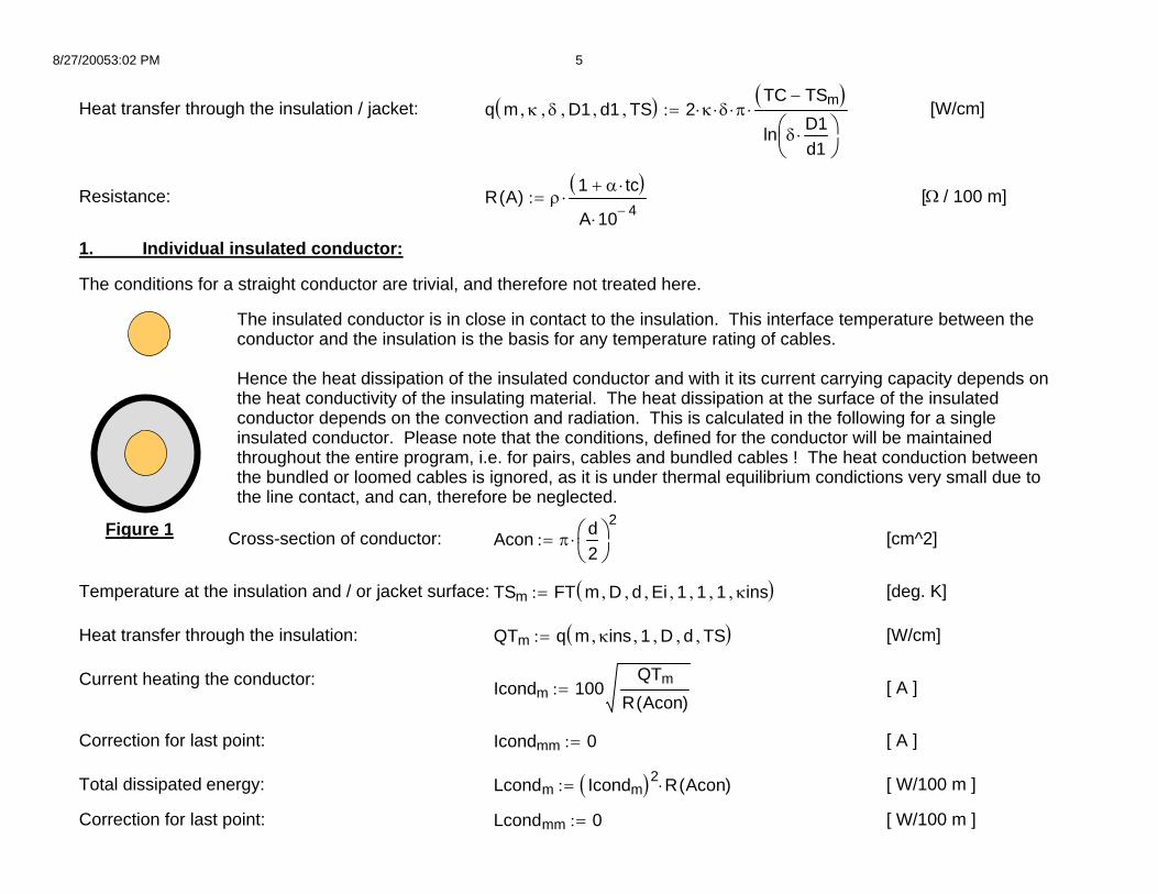
The insulated conductor is in close in contact to the insulation. This interface temperature between the conductor and the insulation is the basis for any temperature rating of cables.

Hence the heat dissipation of the insulated conductor and with it its current carrying capacity depends on the heat conductivity of the insulating material. The heat dissipation at the surface of the insulated conductor depends on the convection and radiation. This is calculated in the following for a single insulated conductor. Please note that the conditions, defined for the conductor will be maintained throughout the entire program, i.e. for pairs, cables and bundled cables ! The heat conduction between the bundled or loomed cables is ignored, as it is under thermal equilibrium condictions very small due to the line contact, and can, therefore be neglected.

The conditions for a straight conductor are trivial, and therefore not treated here.

1. Individual insulated conductor:

[Ω / 100 m]R A( ) ρ1 α tc⋅+( )A 10 4−⋅

⋅:=Resistance:

[W/cm]q m κ, δ, D1, d1, TS,( ) 2 κ⋅ δ⋅ π⋅TC TSm−( )ln δ

D1d1⋅⎛⎜

⎝⎞⎟⎠

⋅:=Heat transfer through the insulation / jacket:

8/27/20053:02 PM 6

Temperature at the wire insulation surface: TSm FT m D, d, Ei, μ, η, δ, κins,( ):= [deg. K]

Heat transfer through the insulation: QTm q m κins, δ, D, d, TS,( ):= [W/cm]

Current heating each conductor: Ipairm100

2QTm

R Apair( ):= [ A ]

Correction for last point: Ipairmm 0:= [ A ]

Total dissipated energy per conductor: Lpairm 2 Ipairm( )2⋅ R Apair( )⋅:= [ W/100 m ]

Correction for last point: Lpairmm 0:= [ W/100 m ]

2. Insulated pair:

For a pair of insulated conductors - the same as previously calculated - the following approximations are used which yield maximum current transfer. In fasct they neglect some generated heat, which will have to be taken otherwise into account. In fact they would result in an additional heating of the conductors and would require an increased heat dissipation into the environment.

Relative circumference for radiation: μ53

:= [ - ]

Relative circumference: ηπ 4+

π:= [ - ]

Equivalent relative circumference ratio: δπ 2+

π:= [ - ]

Figure 2Cross section of the conductors of the pair: Apair 2 Acon⋅:= [cm^2]

The convection is approximated by the combined assumption of an oval and / or an equivalent logarithmic ratio of the equivalent diameters of an insulated conductor to an equivalent conductor diameter.

The radiation is calculated taking the reduction of the radiating part of the circumference into account, where the wires heat themselves mutually by radiation. However, this part, contributing the heat increase of the insulated conductor is here neglected as it is negligibly small especially under thermal equilibrium conditions. Hence we have :

8/27/20053:02 PM 7

[ - ]η5π 12+

π:=Relative circumference:

μ193

8 atan 1

7 4 2⋅+⎛⎜⎝

⎞⎟⎠

⋅⎛⎜⎝

⎞⎟⎠

π−

⎡⎢⎢⎣

⎤⎥⎥⎦

:=Relative circumference for radiation:[ - ]

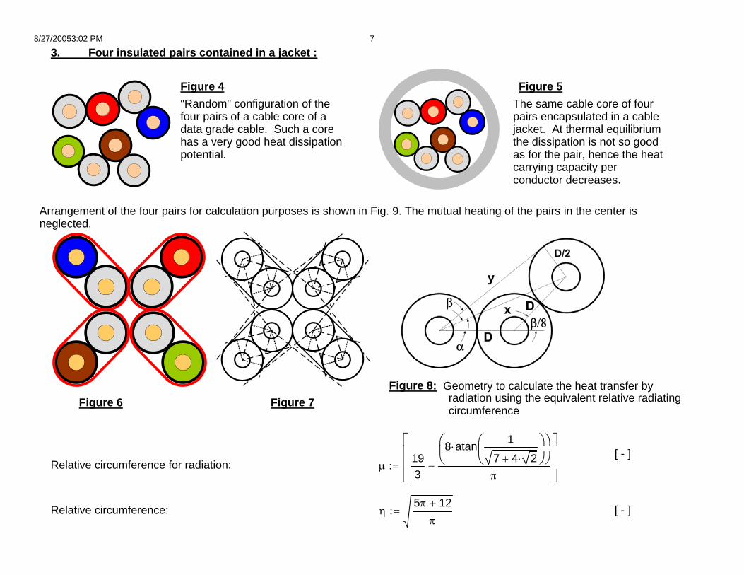
Figure 7Figure 6Figure 8: Geometry to calculate the heat transfer by radiation using the equivalent relative radiating circumference

Arrangement of the four pairs for calculation purposes is shown in Fig. 9. The mutual heating of the pairs in the center is neglected.

The same cable core of four pairs encapsulated in a cable jacket. At thermal equilibrium the dissipation is not so good as for the pair, hence the heat carrying capacity per conductor decreases.

"Random" configuration of the four pairs of a cable core of a data grade cable. Such a core has a very good heat dissipation potential.

Figure 5Figure 4

3. Four insulated pairs contained in a jacket :

8/27/20053:02 PM 8

Conductor Material

Insulation Material

Jacket Material

Equivalent cable model: As model for the assembled cable we use the model shown in Fig. 9.

The overall dimensions of the jacket according to the sketch are much smaller than the realistic jacket dimension. Here we use the real jacket dimensions.

To solve the steady state heat transfer problem to find temperature on the surface of the jacket we use an equivalent conductor model as indicated in the lower part of Fig. 9.

Figure 9

Hollow space,in thermal

equilibrium at temperature of conductor

4. Four insulated pairs encapsulated in a jacket :

[ W/100 m ]Lcoremm 0:=Correction for last point:

[ W/100 m ]Lcorem 8 Icorem( )2⋅ R Acore( )⋅:=Total dissipated energy per conductor:

[ A ]Icoremm 0:=Correction for last point:

[ A ]Icorem100

8QTm

R Acore( ):=Current heating each conductor:

[W/cm]QTm q m κins, δ, D, d, TS,( ):=Heat transfer through the insulation:

[deg. K]TSm FT m D, d, Ei, μ, η, δ, κins,( ):=Temperature at the insulation surface:

[ cm^2]Acore 4 Apair⋅:=Cross section of all conductors in cable :

The temperature of the cable is calculated in two steps, first the temperature increase of the pairs, forming the cable core. With the generated heat the dissipation through a round jacket is calculated.

[ - ]δ 7π 2+

π⋅:=Equivalent relative circumference ratio:

8/27/20053:02 PM 9

Total dissipated energy per conductor: Lcablem 8 Icablem( )2⋅ R Acab( )⋅:= [ W/100 m ]

Correction for last point : Lcablemm 0:= [ W/100 m ]

Note that the dissipated heat from the entire cable is lower than the heat dissipated from the cable core. This is to be expected as a result of the core configuration, which allows a very good dissipation, and allows as a result a substantially higher current, than would occur in the comparable cable. This difference is in fact even increaseded if we take the inside diameter of the jacket equal to the outside diameter of the "optimal cable" core according to Fig. 9, while maintaining the total amount of jacketing material, as shown in the following.

5. Four insulated pairs encapsulated in the smallest possible size jacket :

The model used to calculate the heat dissipation is the same as in Fig. 14 while only the jacket inside diameter is reduced to their minimal size while the jacket wall thickness is increased to reflect the same amount of jakcet material as before.

dz z:= [cm]

Dz DD2 z2+ dd2−:= [cm]Composite thermal conductivity:

κz z2 7 D2 d2−( )⋅−−⎡⎣ ⎤⎦ κins⋅ DD2 z2+ dd2− z−( ) κjack⋅+

DD2 z2+ dd2− z2 7 D2 d2−( )⋅−−:= [ - ]

Figure 10

Composite thermal conductivity κdd dd2 7 D2 d2−( )⋅−−⎡⎣ ⎤⎦ κins⋅ wj κjack⋅+

wj dd+ dd2 7 D2 d2−( )⋅−−:= [ - ]

Cross-section of all conductors in configuration: Acab Acore:= [cm^2]

Temperature at the insulation / cable surface: TSm FT m DD, dd, Ej, 1, 1, 1, κ,( ):= [deg. K]

Heat transfer through the insulation and the jacket: QTm q m κ, 1, DD, dd, TS,( ):= [W/cm]

Current heating each conductor : Icablem100

8QTm

R Acab( ):= [ A ]

Correction for last point : Icablemm 0:= [ A ]

8/27/20053:02 PM 10

Figure 12: Energy to be dissipated per conductor Figure 11: Maximum current per conductor

55 60 65 70 750

50

100

150

Min. Jacket Four Pair Cable Normal Four Pair Cable Cable Core

Ambient temperature [ deg. C ]

Dis

sipa

ted

ener

gy [

W /

100

m ]

55 60 65 70 750

1

2

3

4

Min. Jacket Four Pair Cable Normal Four Pair Cable Cable Core

Ambient temperature [ deg. C ]

Con

duct

or c

urre

nt

[ A ]

[ W/100 m ]Lcminmm 0:=Correction for last point:

[ W/100 m ]Lcminm 8 Icminm( )2⋅ R Acab( )⋅:=Total dissipated energy per conductor:

[ A ]Icminmm 0:=Correction for last point:

[ A ]Icminm100

8QTm

R Acab( ):=Current heating each conductor:

[W/cm]QTm q m κ, 1, Dz, dz, TS,( ):=Heat transfer through the insulation and the jacket:

[deg. K]TSm FT m Dz, dz, Ej, 1, 1, 1, κ,( ):=Temperature at the cable jacket surface:

8/27/20053:02 PM 11

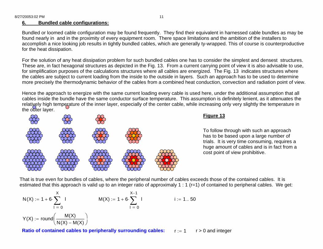
6. Bundled cable configurations:

Bundled or loomed cable configuration may be found frequently. They find their equivalent in harnessed cable bundles as may be found nearly in and in the proximity of every equipment room. There space limitations and the ambition of the installers to accomplish a nice looking job results in tightly bundled cables, which are generally ty-wrapped. This of course is counterproductive for the heat dissipation.

For the solution of any heat dissipation problem for such bundled cables one has to consider the simplest and densest structures. These are, in fact hexagonal structures as depicted in the Fig. 13. From a current carrying point of view it is also advisable to use, for simplification purposes of the calculations structures where all cables are energized. The Fig. 13 indicates structures where the cables are subject to current loading from the inside to the outside in layers. Such an approach has to be used to determine more precisely the thermodynamic behavior of the cables from a combined heat conduction, convection and radiation point of view.

Hence the approach to energize with the same current loading every cable is used here, under the additional assumption that all cables inside the bundle have the same conductor surface temperature. This assumption is definitely lenient, as it attenuates the relatively high temperature of the inner layer, especially of the center cable, while increasing only very slightly the temperature in the outer layer.

Figure 13

To follow through with such an approach has to be based upon a large number of trials. It is very time consuming, requires a huge amount of cables and is in fact from a cost point of view prohibitive.

That is true even for bundles of cables, where the peripheral number of cables exceeds those of the contained cables. It is estimated that this approach is valid up to an integer ratio of approximaly 1 : 1 (r=1) of contained to peripheral cables. We get:

N X( ) 1 60

X

l

l∑=

⋅+:= M X( ) 1 60

X 1−

l

l∑=

⋅+:= i 1 50..:=

Y X( ) round M X( )N X( ) M X( )−⎛⎜⎝

⎞⎟⎠

:=

Ratio of contained cables to peripherally surrounding cables: r 1:= r > 0 and integer

8/27/20053:02 PM 12

[ - ]δπ 6+

π:=Equivalent relative circumference ratio:

[ - ]ηπ 12+ 2 3⋅+

π:=Relative circumference:Figure 14

[ - ]μ 3:=Relative circumference for radiation:

In a the six around one cable configuration all cables are subject to the same current loading. The treatment is straight forward and follows the schematics applied to the cable core. However, it has to be noted here that in this case the bundling or looming of the cables yields a very poor heat dissipation potential. Therefore, for simplicity reasons and as mentioned above, it is assumed that the cable in the center has the same "conductor surface temperature" as the surrounding cables. This would yield too optimistic results, especially with respect to the central cable. The central cable dissipates its internally generated heat exclusively through the surrounding cables, which in turn are themselves heated.Therefore, the current is additionally downrated by a factor of 0.75 per cable layer.

7. Six around one cable configuration :

Note: At the end of this contribution the procedure to be followed is line out if the conductor surface of the innermost cable hasto be limited to the maximum permissible conductor surface temperature, while the conductor temperatures of the surrounding cables have a lower conductor surface temperature due to better dissipation.

Cables we may expect that the derivations presented here will hold nicely.N 37=

N N C( ):=That means up to a cable bundle with

C

x Ak←

break Ak 0=if

k

k 50 1..∈for

k

:=

Ai Y i( ) r−:=

Note: it is left to the daring user to increase eventually this ratio

8/27/20053:02 PM 13

[ W/100 m ]

Correction for last point : Lcab61mm 0:= [ W/100 m ]

7. Eighteen around one cable configuration :

In the Fig. 15 are indicated the geometries which will have to be followed for the calculation. We get:

Relative circumference for radiation: μ 5:= [ - ]

Relative circumference: ηπ 24+ 12 3⋅+

π:= [ - ]

Equivalent relative circumference ratio: δπ 12+

π:= [ - ]

Cross section of all conductors: Acab181 19 Acab⋅:= [ cm^2 ]

Figure 15

Composite thermal conductivity of insulation and jacket: κdd dd2 7 D2 d2−( )⋅−−⎡⎣ ⎤⎦ κins⋅ wj κjack⋅+

wj dd+ dd2 7 D2 d2−( )⋅−−:= [ - ]

Temperature at the outer cable jacket surfaces: TSm FT m DD, dd, Ej, μ, η, δ, κ,( ):= [deg. K]

Cross section of all conductors: Acab61 7 Acab⋅:= [ cm^2]

Heat transfer through the outer jackets: QTm q m κ, δ, DD, dd, TS,( ):= [W/cm]

Current heating each conductor: Icab61m7556

QTm

R Acab61( ):= [ A ]

Correction for last point : Icab61mm 0:= [ A ]

Total dissipated energy per conductor: Lcab61m 56 Icab61m( )2⋅ R Acab61( )⋅:=

8/27/20053:02 PM 14

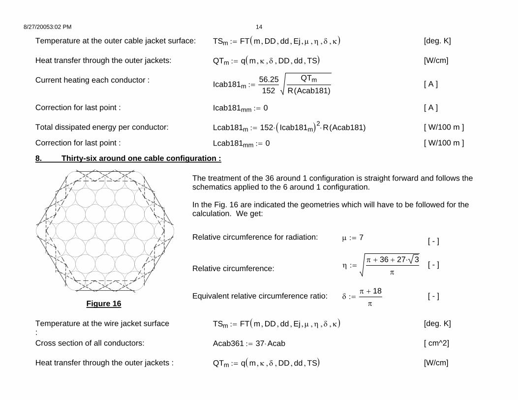
The treatment of the 36 around 1 configuration is straight forward and follows the schematics applied to the 6 around 1 configuration.

In the Fig. 16 are indicated the geometries which will have to be followed for the calculation. We get:

Relative circumference for radiation: μ 7:= [ - ]

ηπ 36+ 27 3⋅+

π:= [ - ]Relative circumference:

Equivalent relative circumference ratio: δπ 18+

π:= [ - ]

Figure 16

Temperature at the wire jacket surface :

TSm FT m DD, dd, Ej, μ, η, δ, κ,( ):= [deg. K]

Cross section of all conductors: Acab361 37 Acab⋅:= [ cm^2]

Heat transfer through the outer jackets : QTm q m κ, δ, DD, dd, TS,( ):= [W/cm]

Temperature at the outer cable jacket surface: TSm FT m DD, dd, Ej, μ, η, δ, κ,( ):= [deg. K]

Heat transfer through the outer jackets: QTm q m κ, δ, DD, dd, TS,( ):= [W/cm]

Current heating each conductor : Icab181m56.25152

QTm

R Acab181( ):= [ A ]

Correction for last point : Icab181mm 0:= [ A ]

Total dissipated energy per conductor: Lcab181m 152 Icab181m( )2⋅ R Acab181( )⋅:= [ W/100 m ]

Correction for last point : Lcab181mm 0:= [ W/100 m ]

8. Thirty-six around one cable configuration :

8/27/20053:02 PM 15

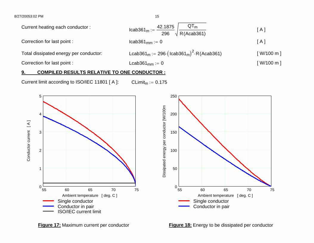
Figure 18: Energy to be dissipated per conductor Figure 17: Maximum current per conductor

55 60 65 70 75

0

50

100

150

200

250

Single conductorConductor in pair

Ambient temperature [ deg. C ]

Dis

sipa

ted

ener

gy p

er c

ondu

ctor

[W/1

00m

55 60 65 70 750

1

2

3

4

5

Single conductorConductor in pairISO/IEC current limit

Ambient temperature [ deg. C ]

Con

duct

or c

urre

nt

[ A ]

CLimitm 0.175:=Current limit according to ISO/IEC 11801 [ A ]:

9. COMPILED RESULTS RELATIVE TO ONE CONDUCTOR :

[ W/100 m ]Lcab361mm 0:=Correction for last point :

[ W/100 m ]Lcab361m 296 Icab361m( )2⋅ R Acab361( )⋅:=Total dissipated energy per conductor:

[ A ]Icab361mm 0:=Correction for last point :

[ A ]Icab361m42.1875

296QTm

R Acab361( ):=Current heating each conductor :

8/27/20053:02 PM 16

55 60 65 70 750

1

2

3

4

5

Single conductorConductor in pairConductor in coreConductor in cableISO/IEC current limit

Ambient temperature [ deg. C ]

Dis

sipa

ted

ener

gy p

er c

ondu

ctor

[W/1

00m

55 60 65 70 750

1

2

3

4

Conductor in coreConductor in cableConductor in a 6 around 1 configurationConductor in a 18 around 1 configurationConductor in a 36 around 1 configurationISO/IEC current limit

Ambient temperature [ deg. C ]

Con

duct

or c

urre

nt

[ A ]

Figure 19: Maximum current per conductor Figure 20: Maximum current per conductor

8/27/20053:02 PM 17

0 1 2 3 4 50

0.1

0.2

0.3

0.4

0.5

0.6

0.7

Conductor in a 6 around 1 configurationConductor in a 18 around 1 configurationConductor in a 36 around 1 configurationISO/IEC current limit

"Rated" minus ambient temp. [ deg. C ]

Con

duct

or c

urre

nt

[ A ]

0 1 2 3 4 50

0.5

1

1.5

2

Single conductorConductor in pairConductor in coreConductor in cableISO/IEC current limit

"Rated" minus ambient temp. [ deg. C ]

Dis

sipa

ted

ener

gy p

er c

ondu

ctor

[W/1

00m

Figure 21: Maximum current per conductor Figure 22: Maximum current per conductor

8/27/20053:02 PM 18

10. Indications about the comprehensive solution of the presented problem:

Jacket Material

Insulation Material

Conductor Material

Center cable or layer

Proportion of diameter of heat transfer through the insulation of the conductors of the first layer and the jacket material to the jacket surfaces of the outer cables of the first layer Figure 24: Explanation of the fractions

for the calculation of the proportions of the diameters participating in the heatdissipation of the central cable or the central bundle

Proportion of diameter of direct heat transfer from the inner cable or bundle through the jacket material to the jacket surfaces of the outer cables of the first layer

Figure 23

After determination of the angular portion of the dissipation of the heat through the part of the jacket material and consecutively through the jacket and insulation material, we can compute the heat disspation through these sections. We can assume circular configurations for the heat transfer from the inner (central) cable or layer through the jacket. We can assume as the same condicitons also for the heat dissipation through the insulation and jacket, and also for the remaining heat transfer through the insulated conductors of the outer layer all over the outer jacket into the environment. In this case the heat transfer into the outer layer increases the heat in the outer layer over the one generated by the current. As a result the surface temperature of the conductors of the central cable is the one exposed to the current limitation of the entire cable bundle.

To determine the geometries for all configurations used above is tedious, and goes definitely beyond the author's actual patience to deal with this problem.

8/27/20053:02 PM 19

Saving of data to desktop:

C:\..\data

augment ta Icore, Icable, Icab61, Icab181, Icab361, CLimit,( )

11. References :

[1] Steve Meyer : Wire TableNaval Air Weapons CenterCode 543400DChina Lake, CA 93555(619)-939-6005steve_meyer@rccgw.chinalake.navy.mil

[2] J.- H. Walling: Current carrying capacity of data grade cablesContributuion to IEEE 802.3af : walling_1_0305