Wright State University Wright State University

CORE Scholar CORE Scholar

Browse all Theses and Dissertations Theses and Dissertations

2010

The Harmonic Distortion Reduction of Phase-Angle Fired SCRs The Harmonic Distortion Reduction of Phase-Angle Fired SCRs

Feeding a Resistive Load using Fuzzy Logic Feeding a Resistive Load using Fuzzy Logic

Matthew A. Clark Wright State University

Follow this and additional works at: https://corescholar.libraries.wright.edu/etd_all

Part of the Electrical and Computer Engineering Commons

Repository Citation Repository Citation Clark, Matthew A., "The Harmonic Distortion Reduction of Phase-Angle Fired SCRs Feeding a Resistive Load using Fuzzy Logic" (2010). Browse all Theses and Dissertations. 330. https://corescholar.libraries.wright.edu/etd_all/330

This Thesis is brought to you for free and open access by the Theses and Dissertations at CORE Scholar. It has been accepted for inclusion in Browse all Theses and Dissertations by an authorized administrator of CORE Scholar. For more information, please contact library-corescholar@wright.edu.

The Harmonic Distortion Reduction of Phase-AngleFired SCRs Feeding a Resistive Load using Fuzzy

Logic

A thesis submitted in partial fulfillmentof the requirements for the degree of

Master of Science in Engineering

by

Matthew A. ClarkB.S.E.E, Wright State University, 2000

2010Wright State University

Wright State UniversitySCHOOL OF GRADUATE STUDIES

April 12, 2010

I HEREBY RECOMMEND THAT THE THESIS PREPARED UNDER MY SUPER-VISION BY Matthew A. Clark ENTITLED The Harmonic Distortion Reduction of Phase-AngleFired SCRs Feeding a Resistive Load using Fuzzy Logic BE ACCEPTED IN PARTIALFULFILLMENT OF THE REQUIREMENTS FOR THE DEGREE OF Master of Sciencein Engineering.

Kuldip S. Rattan, Ph.D.Thesis Director

Kefu Xue, Ph.D.Department Chair

Committee onFinal Examination

Kuldip S. Rattan, Ph.D.

Marian Kazimierczuk, Ph.D.

Xiaodong Zhang, Ph.D.

John A. Bantle, Ph.D.Vice President for Research andGraduate Studies and Interim Deanof Graduate Studies

ABSTRACT

Clark, Matthew. M.S.Egr., , Wright State University, 2010. The Harmonic Distortion Reduction ofPhase-Angle Fired SCRs Feeding a Resistive Load using Fuzzy Logic.

High power silicon controlled rectifiers (SCR) are used in the application of infrared

radiation testing. A case study has been performed on a department of defense facility

utilizing SCRs to transfer electrical energy to thermal energy. The facility is capable of

generating up to 5000 ◦F across large cross-sectional areas, requiring tens of megawatts

of power. The combination of high power, unbalanced loads, and SCR switching gen-

erate high harmonic disturbances that offer significant challenges for conventional linear

control systems. In addition, unbalanced three-phase distribution systems are difficult to

model, specifically during switching transients. Fuzzy logic is used to characterize the

non-linear plant dynamics, control the system output, and reduce harmonics. Although the

use of fuzzy logic for harmonic reduction has been used extensively in the power industry,

most applications focus on compensating for harmonic disturbance rather than avoiding it.

Harmonic compensation adds hardware in the system, which adds maintenance costs and

inefficiency. This thesis introduces a technique to eliminate harmonic content in the con-

trol loop without adding additional hardware. A simulation of the system was created and

fuzzy logic was used to characterize the behavior of the simulation. The simulation results

demonstrated the non-linear control problem and identified key harmonic areas to avoid.

A fuzzy proportional-integral controller along with a fuzzy harmonic reduction controller

is implemented in this thesis to improve the control response while avoiding harmful har-

monic interference. The fuzzy harmonic reduction controller yielded a hybrid pulse width

modulation output that eliminated the most harmful harmonics while maintaining closed

loop control.

iii

List of SymbolsChapter 1

Q Heat FluxA Area of a radiating bodyε Emissivityσ Stefan-Boltzman constant 5.67x10−8W/m2K4

iv

Contents

1 Introduction 11.1 Problem Definition . . . . . . . . . . . . . . . . . . . . . . . . . . . . . . 11.2 Proposed Solution . . . . . . . . . . . . . . . . . . . . . . . . . . . . . . . 9

2 Significance of Research 112.1 Motivation . . . . . . . . . . . . . . . . . . . . . . . . . . . . . . . . . . . 11

2.1.1 Case Study Background . . . . . . . . . . . . . . . . . . . . . . . 112.1.2 Case Study Requirements . . . . . . . . . . . . . . . . . . . . . . 14

2.2 Harmonic Mitigation Options . . . . . . . . . . . . . . . . . . . . . . . . . 172.2.1 Implement Passive Circuits . . . . . . . . . . . . . . . . . . . . . . 182.2.2 Multi-phasing of Load via an IGBT . . . . . . . . . . . . . . . . . 182.2.3 Switch the SCRs to Zero-Cross Technology . . . . . . . . . . . . . 182.2.4 Active Line Compensation . . . . . . . . . . . . . . . . . . . . . . 19

3 System Modeling 213.1 The Silicon Controlled Rectifier . . . . . . . . . . . . . . . . . . . . . . . 213.2 The Transformer and Total Loads . . . . . . . . . . . . . . . . . . . . . . . 26

4 Introduction to Fuzzy Logic 304.1 Fuzzy Sets . . . . . . . . . . . . . . . . . . . . . . . . . . . . . . . . . . . 314.2 Fuzzy Partitioning . . . . . . . . . . . . . . . . . . . . . . . . . . . . . . . 334.3 Linguistic variables . . . . . . . . . . . . . . . . . . . . . . . . . . . . . . 344.4 Fuzzy Rules . . . . . . . . . . . . . . . . . . . . . . . . . . . . . . . . . . 354.5 Fuzzy Control . . . . . . . . . . . . . . . . . . . . . . . . . . . . . . . . . 35

5 Fuzzy Logic Implementation 405.1 Plant Characterization using Fuzzy Logic . . . . . . . . . . . . . . . . . . 405.2 The PI Controller Implementation . . . . . . . . . . . . . . . . . . . . . . 51

5.2.1 The Radiant Heat System Plant . . . . . . . . . . . . . . . . . . . 515.2.2 The Initial Linear Controller . . . . . . . . . . . . . . . . . . . . . 595.2.3 The Fuzzy PI Controller . . . . . . . . . . . . . . . . . . . . . . . 64

5.3 The Fuzzy Harmonic Reduction Controller . . . . . . . . . . . . . . . . . 69

v

6 Conclusions 79

Bibliography 81

7 Appendix A: Matlab Code 84

vi

List of Figures

1.1 Single phase, phase angle fired SCR representative circuit. . . . . . . . . . 21.2 Representative circuit of three single phase SCRs connected in a Delta

Load configuration, fed by a Delta transformer. . . . . . . . . . . . . . . . 31.3 RMS Power of uncontrolled single phase ignitron with graphite heater load. 41.4 Result of SCR prematurely turning off due to phase A and B combined

transient spike. . . . . . . . . . . . . . . . . . . . . . . . . . . . . . . . . 51.5 Result of SCR prematurely turning on due to phase A and B combined

transient spike. . . . . . . . . . . . . . . . . . . . . . . . . . . . . . . . . 51.6 Line side transients from SCR firing at complementary phases 45,90,135 ◦. 61.7 Load side transients from SCR firing at complementary phases 45,90,135 ◦. 71.8 GASMG Schematic of a 600V delta-delta transformer and delta loads. . . . 8

2.1 Graphite heater array. . . . . . . . . . . . . . . . . . . . . . . . . . . . . . 132.2 Quartz heater array. . . . . . . . . . . . . . . . . . . . . . . . . . . . . . . 132.3 Simultated transformer variances of THD given by the available KVA. . . . 17

3.1 Simulated SCR using ideal switch. . . . . . . . . . . . . . . . . . . . . . . 233.2 Zero Cross Detection for SCR triggering. . . . . . . . . . . . . . . . . . . 273.3 One dimensional model representation of transient TURN ON current effects. 283.4 Graph of single phase line and load voltages with and without SCR snubber

present. . . . . . . . . . . . . . . . . . . . . . . . . . . . . . . . . . . . . 283.5 Full three phase Delta-Delta transformer. . . . . . . . . . . . . . . . . . . . 29

4.1 Comparison of conventional and fuzzy sets [1]. . . . . . . . . . . . . . . . 314.2 Complement of a fuzzy set [1]. . . . . . . . . . . . . . . . . . . . . . . . . 324.3 Union of two fuzzy sets [1]. . . . . . . . . . . . . . . . . . . . . . . . . . 324.4 Intersection of two fuzzy sets using the product method [2]. . . . . . . . . . 334.5 Fuzzy partitioning of a phase angle space U . . . . . . . . . . . . . . . . . . 344.6 Fuzzy linguistic variables of coffee pouring rate [1]. . . . . . . . . . . . . . 354.7 Block diagram of the fuzzy controller [2]. . . . . . . . . . . . . . . . . . . 364.8 An example of fuzzification. . . . . . . . . . . . . . . . . . . . . . . . . . 374.9 Min-Max method of inference to produce fuzzy sets [1]. . . . . . . . . . . 38

5.1 Representation of the plant inputs and outputs. . . . . . . . . . . . . . . . . 41

vii

5.2 Representation of the plant input fuzzification. . . . . . . . . . . . . . . . . 415.3 Representation of the plant output fuzzification. . . . . . . . . . . . . . . . 415.4 Fuzzification of crisp phase angle values. . . . . . . . . . . . . . . . . . . 435.5 Fuzzification of crisp % VRMS error values. . . . . . . . . . . . . . . . . . 445.6 Fuzzification of crisp THD values. . . . . . . . . . . . . . . . . . . . . . . 445.7 VRMS vs phase α with varied loads. . . . . . . . . . . . . . . . . . . . . . 455.8 % VRMS error of each transformer phase vs SCR phase angle combinations. 465.9 THD of each each transformer phase vs SCR phase angle combinations. . . 475.10 Standard deviation of %VRMS error of each transformer phase vs SCR

phase angle combinations. . . . . . . . . . . . . . . . . . . . . . . . . . . 485.11 THD vs phase α with varied loads. . . . . . . . . . . . . . . . . . . . . . . 505.12 THD of each φ vs phase α with a single phase 400KW load. . . . . . . . . 515.13 Representative SCR inner loop. . . . . . . . . . . . . . . . . . . . . . . . . 525.14 Representative heat transfer from heating element to test article. . . . . . . 535.15 Representative heat transfer from heating element to test article resultant

graph. . . . . . . . . . . . . . . . . . . . . . . . . . . . . . . . . . . . . . 545.16 Open loop plant with SCR, heater, and simulated plant. . . . . . . . . . . . 555.17 Representative SCR inner model. . . . . . . . . . . . . . . . . . . . . . . . 565.18 Drive% vs. Telement(

◦F ). . . . . . . . . . . . . . . . . . . . . . . . . . . . 575.19 VRMS and PRMS with respect to drive %. . . . . . . . . . . . . . . . . . . . 585.20 Simulink model of the representative analog control system . . . . . . . . . 595.21 Root locus of the open loop transfer function . . . . . . . . . . . . . . . . 605.22 Simulink model of the analog control system . . . . . . . . . . . . . . . . 635.23 Resultant response of the closed loop classic PI control system. . . . . . . . 645.24 Fuzzy PI controller implementation in Simulink. . . . . . . . . . . . . . . . 655.25 Equally spaced membership functions for the PI controller. . . . . . . . . . 655.26 Rule Base for the standard Fuzzy Proportional Plus Integral Controller. . . . 665.27 Response of the evenly spaced Fuzzy Logic PI controller. . . . . . . . . . . 665.28 The phase angle output of the evenly spaced Fuzzy PI controller. . . . . . . 675.29 Modified Fuzzy PI controller System Response. . . . . . . . . . . . . . . . 685.30 Control Surface for the error signal. . . . . . . . . . . . . . . . . . . . . . 695.31 Resultant phase angle output response of the closed loop classic PI control

system. . . . . . . . . . . . . . . . . . . . . . . . . . . . . . . . . . . . . 705.32 Region of phase angles to be avoided to minimize harmonics. Classical

controller response shown in the avoidance region. . . . . . . . . . . . . . 705.33 Control surface for harmonic mitigation controller. . . . . . . . . . . . . . 725.34 Close up of the harmful harmonic region in the control surface for harmonic

mitigation controller. . . . . . . . . . . . . . . . . . . . . . . . . . . . . . 735.35 Error membership function for the harmonic mitigation controller. . . . . . 735.36 Output membership function for the harmonic mitigation controller. . . . . 735.37 Complete system with harmonic mitigation fuzzy Controller. . . . . . . . . 755.38 Resultant phase control output with and without harmonic reduction con-

troller. . . . . . . . . . . . . . . . . . . . . . . . . . . . . . . . . . . . . . 765.39 Resultant phase control output with harmonic reduction controller. . . . . . 765.40 Resultant output response with the harmonic reduction controller . . . . . . 77

viii

5.41 Close up of figure 5.38, visualizing the switching mode of controller. . . . . 77

ix

List of Tables

5.1 Combinations of fuzzification centers for rule generation. . . . . . . . . . . 49

x

AcknowledgmentI would like to extend my thanks Dr. Rattan for all his help with this project. Also for

Jim Combs for the expert instruction on the content of Radiant Heat Testing and Control.

Without his knowledge this thesis would not be possible. Finally, my wife and children

have been more than patient and enduring. For that, I am sincerely grateful.

xi

Dedicated to

My Wife, Julie

xii

Introduction

1.1 Problem Definition

The rise of switching technology has introduced a major field of study in harmonic suppres-

sion in power electronics. Large industrial facilities suffer from not only the requirements

to maintain a total harmonic distortion content below the standard IEEE std 519 guide-

lines, but also suffer from the ability to control and maintain operation due to multiple

system harmonic interplay [3] [4].

As switch technology grows and becomes more and more prevalent, total harmonic

distortion (THD) has become an increasingly difficult problem with varied solution alterna-

tives. Research has been performed to discover some of the techniques used in mitigating

THD in various industrial settings. This thesis presents a novel approach to dynamically

avoid problematic regions of distortion that may cause inerrant control of single phase sili-

con controlled rectifiers.

Silicon controlled rectifiers (SCR) are the mainstay of many industrial applications.

Their applications range from electric welders to high voltage AC to DC rectifiers to large

1

variable frequency motor drives (VFD)s. They are found in almost every field from loco-

motives to high speed transmission line switches. SCRs are primarily used for low speed,

high voltage and high current switching [5]. Not unique to their use is the United States

Government for the purposes of research and testing. NASA, the department of defense,

and the department of energy all use large SCR banks control resistive heating elements for

the purpose of radiative thermal testing with powers exceeding 30-50 MW.

A particular case study of a defense research facility offers a basis for this research

and motivation for this thesis. A back to back silicon controlled rectifier circuit provides

varied power to a load by only allowing a percentage of positive and negative AC sine

wave to be active. This percentage is achieved by allowing SCR conduction only past

specific phase angle, from 0 to 180◦ radians. This yields a sine wave that is off for one

portion of its period and then on for the rest. The cut wave delivers proportional radiant

energy to the test article by producing an equivalent root mean square (RMS) power across

a resistive heating element. Figure 1.1 displays the phase angle fired SCR equivalent circuit

and corresponding voltage sine wave. The shaded region represents the SCR “ON-TIME”.

Figure 1.1: Single phase, phase angle fired SCR representative circuit.

Problems can arise in the configuration of these devices and the total radio frequency

interference produced by the transient switching. This transient switching can produce

undesirable controller results if two or more devices switch at the same time, causing an

2

SCR to “turn-off” prematurely [6]. Historically, only two of the three single phase SCRs,

fed from the same substation, could be fired if graphite heating elements were used. This

phenomenon is thought to be due to the harmonic disturbances induced by the sharp step

of the ignitron or SCR. Figure 1.2 displays the total system from transformer secondary to

the delta configured SCR and load combination.

Figure 1.2: Representative circuit of three single phase SCRs connected in a Delta Loadconfiguration, fed by a Delta transformer.

The A, B, C is phase designation of the load. The output voltage shown in figure 1.1

is measured from A to B, B to C, and C to A for channels 1 to 3 respectively. The RMS

voltage, power, and current transducers used for closed loop control is measured across

the load. Figure 1.3 displays the representative data, demonstrating the loss of control at

a point in the heat profile. The control loop in this example was using RMS power as the

feedback. The apparent harmonic effect of all three SCRs firing is thought to create a back

feed from one phase to another.

As a test profile is realized across three co-joined single phase SCRs, a region exists

where two or more SCRs fire at the same time. This occurs only when two channels are

transitioning from off state to on state at the same time. The sum of the two phases causes

a transient spike, due to the nature of the delta-delta transformer, circulates through the

3

Figure 1.3: RMS Power of uncontrolled single phase ignitron with graphite heater load.

windings and is manifested on the third SCR as a reverse bias (see figure 1.4 [5]. The

TURN-ON time of the SCR (referred to in figure 1.4 as tq) is the minimum amount of time

the input voltage must reverse bias the SCR to turn the device off. The transient caused by

harmonic distortion is thought to be sufficiently longer than tq, thereby turning the device

off [5].

Similarly, the total harmonic distortion could also feed into the firing circuit in the

form of noise, triggering the third SCR to prematurely turn on. Notice in figure 1.5, how

phase C SCR is on for a complete half cycle.

In 2007, a simulation of the power system was carried out to observe the relationship

of phase harmonics circulating through the Delta-Delta transformer. A program written for

the propulsions directorate at Wright Patterson AFB was used to model the transformer and

4

Figure 1.4: Result of SCR prematurely turning off due to phase A and B combined transientspike.

Figure 1.5: Result of SCR prematurely turning on due to phase A and B combined transientspike.

three phase, unbalanced, switching characteristics of the case study. The Graphical Auto-

mated State Model Generator (GASMG) was used in conjunction with MATLAB 2006b.

5

GASMG is a software package developed by PC Krause and Associates that generates the

state-space model of a SPICE-like circuit, feeding it back into a Simulink model [7]. Figure

1.8 shows the representative circuit simulated in GASMG. This model was able to capture

some of the transient events present in the system, including noise, delay, and harmonics

induced by the switching of the SCRs. Figure 1.6 displays the switching effects of the

SCRs on the secondary line side of the transformer, while figure 1.7 displays the load ef-

fects. Notice how the SCR step on one phase induces voltage dips on the line feeding the

other phases.

Figure 1.6: Line side transients from SCR firing at complementary phases 45,90,135 ◦.

6

Figure 1.7: Load side transients from SCR firing at complementary phases 45,90,135 ◦.

7

Figure 1.8: GASMG Schematic of a 600V delta-delta transformer and delta loads.

8

The true instability is realized when a control loop is used in conjunction with the

SCR bank. Either condition above delivers more than or less than total RMS power to the

load than is expected. The difference translates directly into control system error. In radiant

heat testing, most control loops utilize either test article surface temperature, power, or heat

flux as the feedback mechanism. At the point where the transient allows the third SCR to

prematurely turn off or on, the total RMS on phase C is more than or less than the power

expected, causing errant, unsuspecting control. Figure 1.3 displays a condition where the

third channel went out of control only at a specific set of conditions.

1.2 Proposed Solution

It has been observed by simulation that the most severe harmonics are generated when an

SCR is activated somewhere between 70◦ and 100◦ phase angle. The solution proposed in

this paper is to use a non-linear control method to minimize the harmonics induced onto the

system. A fuzzy logic controller would yeild the effects of realizing the same total RMS

equivalent power over two cycles while avoiding a range of phase angle combinations that

produced the most damaging harmonics. Fuzzy logic is the proposed method due to its

ability, through fuzzy partitions, eliminate harmful harmonics while maintaining proper

control. The goal of this thesis is to demonstrate that at fuzzy logic controller can enable

three or more single phase SCR controllers to operate congruently by dynamically reducing

the total harmonic distortion (THD) of the given system. The objective is to synchronize

each controller in order to reduce the degree of complimentary harmonics between phases

and or cancel them. This can be achieved by leveraging that the bandwidth of the system is

much less than switching frequency of the SCR. Due to the constant reconfiguration of the

load, the fuzzy harmonic compensation must be adaptive.

9

This thesis will discuss the significance of this research in the field of power elec-

tronics and control. Secondly, a simulation will be performed to characterize the harmonic

distortion. Once the characterization is performed, a range of phase angles will be identified

to avoid. The control system plant is then modeled to demonstrate a classical controller.

The classical controller is replaced by a fuzzy proportional plus integral controller. Then a

harmonic mitigation controller is added to the model to demonstrate harmonic elimination.

The results show no loss of plant controllability with the elimination of harmful harmonics.

10

Significance of Research

2.1 Motivation

2.1.1 Case Study Background

Infrared radiant heat testing is used for the analysis of structures in extreme temperature

environments for flight vehicles. Although dissimilar, a correlation can be made between

aerodynamic heating and radiant infrared heating [8]. This correlation is useful in vali-

dating aerodynamic design considerations. An aerodynamic structure may be required to

withstand frictional transient temperatures in excess of 5000 ◦F. It is imperative to test ther-

mal protection systems (such as shuttle tiles) or the effect of unequal thermal expansion on

aeronautical vehicles.

In the 1960s, evaluations were made at the flight structural testing facilities at Wright

Patterson Air Force Base to perform high temperature radiant heat testing [9]. The need

existed and still exists to have facilities that are capable of producing large radiant heat

11

gradients across a structure. These facilities have since been created and have been widely

successful in demonstrating real flight conditions and validating computer models [8]. The

electrical power distribution for these facilities has not dramatically changed over the last

40 years.

Thermal gradients per unit time are achieved by varying the electrical power applied to

the resistive loads. The resistive elements convert electrical power into infrared radiation.

The infrared radiation emanates from the elements radially from the source to the test article

[9] [10]. The heat flux,Q , is directly proportional to the power, W , provided to the lamp.

The equation (2.1) relates temperature and power from a hot body to a cold one [8].

P = εσA(T 4 − T 4C ) (2.1)

The power system converts electrical energy to heat by transferring proportional power

to a non-linear resistive load. Depending on the temperature range desired, two common

resistive loads are used,

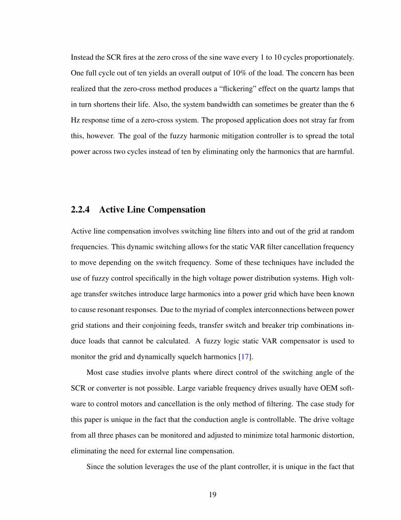
1. Tungsten filamant quartz bulbs, Figure 2.2.

2. Custom designed graphite heating elements, Figure 2.1.

12

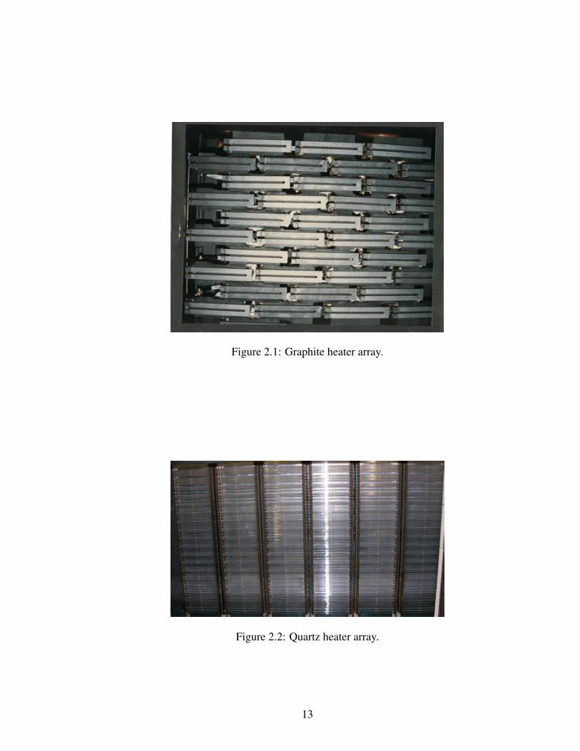
Figure 2.1: Graphite heater array.

Figure 2.2: Quartz heater array.

13

The graphite element (figure 2.1), while in an inert environment, can achieve 4500−

5500 ◦F per module, radiating 350-400 btuft2sec

. The graphite elements are not linear, but

more quadratic in nature. They require approximately 120 V at 700 A each [11]. The

tungsten filament elements (figure 2.2) can achieve test article surface temperatures of less

than 3000 ◦F [9][11]. They require only 13 A at 480 V and can achieve 80-100 btuft2sec

. The

diameter of the quartz tube surrounding the filament prevents the quartz lamp to achieve

the flux density provided by the graphite heater. However, they are more flexible in the fact

that they do not require an inert environment, are more linear in response, and have a wider

range of reflector configurations available to focus the flux [8].

2.1.2 Case Study Requirements

In 2007, a new facility was designed and installed, replacing the ignitron tubes and a DEC

VAX control system with SCRs and a Modicon PLC control system. In the design of the

new system there are three main requirements.

1. The investment in a radiant heating facility is quite large and therefore must be as

versatile as possible. The available power must be able to be re-configured to apply

the desired heat loads in various zones or configurations with the maximum available

power output per zone being 600KW.

2. The system must be able to control these zones independently and congruently to

enable the exact heat flux distribution of the rate specified.

3. The system must not, through any power modulation technique, create power distur-

bances that can affect the test instrumentation or data collection systems.

The first requirement suggested that the power distribution system should be single

phase in nature in order to offer the most control flexibility per channel. Legacy has much

14

to do with the design of the current system with regards to the types of heating elements.

Before the new installation, the facility utilized ignitron tubes to modulate the power to

resistive heating elements. The switching technology of mercury filled ignitron tubes and

silicon controlled rectifiers are identical. The present resistive heating elements have been

used for over 40 years. Several variants of these heaters have been used in other facilities in

the past including DC driven systems and three phase systems [9]. However, modifying the

power distribution design from single phase to either a three phase system or a DC system

would induce a larger infrastructure change and is not feasible. Empirically, it has been

seen that the harmonic control issue is not present when all three single phase channels on

one distribution system operate synchronously. Thereby, the specific problem of inerrant

control due to unbalanced loading could be eliminated if this requirement did not exist.

The second requirement, and the failure at this time to meet it, directly affects the facil-

ity capability. Not being able to control three phases simultaneously on a given substation

limits the available channels. The power delivery system consists of 24 single phase silicon

controlled rectifiers. Each SCR is powered by a 3 phase, 600 Vac, delta-delta transformers.

Each delta-delta transformer is capable of delivering roughly 2000 kilo-volt amperes and

supplies three single phase 1000A SCRs and three single phase 500A SCRs. Due to the

inability to control three phases per substation at once, if each zone requires independent

control then the overall capability must be extracted using only 2 1000 A channels and 2

500 A channels per substation. This reduces the facility capacity from 24 channels to 16,

or a total reduction of 33%!

The final requirement is to remain compliant with the IEEE standards for total har-

monic distortion. IEEE standard 519 suggests that plant total harmonic distortion be lim-

ited to 5%. It is believed that harmonic distortion mitigation techniques directly relate to

the ability to solve the problem presented. Harmonic distortion is the distortion of the

fundamental sinusoidal wave of a power system. This distortion leads to several system

problems including over heating, voltage drops, ferroresonance, radio frequency distur-

15

bances on precision electrical equipment [12]. Distortion to the sine wave depends heavily

on the ratio of the magnitude of the unbalanced load and the transformer rated KVA. In this

study, a Matlab model of a characteristic transformer was performed. In Chapter 3, more

data is displayed to solidify this.

For data collection and instrumentation systems, great care has been taken to segre-

gate the power distribution systems such that harmonic distortion does not effect external

devices. As stated, the SCR power distribution system is an ungrounded Delta-Delta trans-

former. The unique capability of this transformer is it’s ability to isolate harmonic content

from the rest of the facility. The harmonics generated on the secondary side of the substa-

tion have no where to go but to the other phases. This is referred to as circulating currents or

harmonics [5] [13]. The ungrounded secondary Delta avoids unbalanced, harmonic loads

from inducing zero sequence current into the primary lines.

The harmonic distortion generated by SCRs on a delta-delta transformer does effect

the internal control loops. THD and inerrant control are believed to be related. It is believed

that if the THD can be reduced then the system will be more easily controlled [3]. It has

been found that the primary effect SCRs have on total harmonic distortion is directly related

to the capability of the transformer. The magnitude of the load with respect to the total KVA

of the feeding transformer definitely points to total harmonic distortion. Figure 2.3 displays

the results of the same load with three different KVA rated transformers. In this case the

model starts at 200,000 KVA available power with a single phase load fired from an SCR

at a phase angle of 90 degrees. The load value is 83KVA. It can be easily seen that the total

harmonic distortion is closely related to the transformer capability. This is a significant

fact. The model used for figure 2.3 is the same model used to emulate the current physical

setup. In fact, the substations are only 2,000 KVA rated. Therefore, if a single phase load

were to be used at that capacity, the SCR would not fire correctly at a 90 degree phase

angle.

16

Figure 2.3: Simultated transformer variances of THD given by the available KVA.

2.2 Harmonic Mitigation Options

The detailed description of the existing system, the transient mitigation solutions installed,

and the comparison to the Matlab model have two purposes. Firstly, the system perfor-

mance must be understood to further gain knowledge on how to minimize the total har-

monic distortion, thereby eliminating unpredictable control. Secondly, to make it clear that

the new installation did in fact attempt to mitigate some of control issues. A study has been

carried out to find the alternative options to mitigate harmonics.

17

2.2.1 Implement Passive Circuits

Passive RLC circuits have been introduced into systems to filter known harmonic signals.

Typically, these circuits are designed to eliminate specific frequencies, typically the highest

magnitude triplen harmonics, or odd multiples of the 3rd harmonic [14]. These circuits are

best suited for known harmonic loads where the installation is static or calculated based on

empirical data. If the system configuration changes drastically, the distortion content may

not be stable. Certain conditions may cause the filter to become resonant and destructive

[3] [15]. For this reason, passive filters are not an applicable solution.

2.2.2 Multi-phasing of Load via an IGBT

Another option to be considered would be the introduction of higher switching frequencies.

Presently the SCR proportionately delivers power to the load by cutting the sinusoid only

once per half cycle. If the switching frequency increase to 10-18 kHz or more, the tran-

sients would not be as dramatic. To accomplish this the SCR would need to be replaced

with an IGBT. The advantage to an IGBT would be the higher switching frequency capa-

bility and the very low gate TURN-ON current. Additionally, techniques such as random

switching between phases could be used to reduce the interplay between harmonics [16].

Currently, OEM solutions for 1000 amp single phase IGBTs are not cost effective and were

not available during the SCR installation.

2.2.3 Switch the SCRs to Zero-Cross Technology

Other test agencies perform heat testing with an SCR switching technology referred to

as zero-cross [8]. Simply, the SCR does not cut the wave to produce proportional power.

18

Instead the SCR fires at the zero cross of the sine wave every 1 to 10 cycles proportionately.

One full cycle out of ten yields an overall output of 10% of the load. The concern has been

realized that the zero-cross method produces a “flickering” effect on the quartz lamps that

in turn shortens their life. Also, the system bandwidth can sometimes be greater than the 6

Hz response time of a zero-cross system. The proposed application does not stray far from

this, however. The goal of the fuzzy harmonic mitigation controller is to spread the total

power across two cycles instead of ten by eliminating only the harmonics that are harmful.

2.2.4 Active Line Compensation

Active line compensation involves switching line filters into and out of the grid at random

frequencies. This dynamic switching allows for the static VAR filter cancellation frequency

to move depending on the switch frequency. Some of these techniques have included the

use of fuzzy control specifically in the high voltage power distribution systems. High volt-

age transfer switches introduce large harmonics into a power grid which have been known

to cause resonant responses. Due to the myriad of complex interconnections between power

grid stations and their conjoining feeds, transfer switch and breaker trip combinations in-

duce loads that cannot be calculated. A fuzzy logic static VAR compensator is used to

monitor the grid and dynamically squelch harmonics [17].

Most case studies involve plants where direct control of the switching angle of the

SCR or converter is not possible. Large variable frequency drives usually have OEM soft-

ware to control motors and cancellation is the only method of filtering. The case study for

this paper is unique in the fact that the conduction angle is controllable. The drive voltage

from all three phases can be monitored and adjusted to minimize total harmonic distortion,

eliminating the need for external line compensation.

Since the solution leverages the use of the plant controller, it is unique in the fact that

19

the harmonic elimination is not adding additional hardware, thereby saving maintenance

costs and equipment efficiency losses. To eliminate harmful harmonics programmatically,

the plant must be characterized. This characterization identifies what harmonics are the

most harmful. Once those are characterized, a fuzzy harmonic mitigation controller can

eliminate those frequencies.

20

System Modeling

In order to characterize the system, either real world data must be collected or a simula-

tion must be performed. Due to the costly and potentially harmful nature of real world

experiments, a simulation was created to model the transformer and SCR. It is imperative

to model the three phase interactions to best represent the harmonic issues. The simula-

tion enabled the characterization of the plant and what rule base should be used for fuzzy

control. It should be noted that modeling unbalanced transformer and power distribution

systems is very difficult and well beyond the purpose of this paper. The Matlab model only

serves as a “typical” response as compared to real field data.

3.1 The Silicon Controlled Rectifier

The simulation performed in 2007 using the GASMG software was duplicated using an

evaluation version of Matlab SimPowerSystems. From this software an ideal switch with

a snubber circuit was used to model the SCR 3.1. The load attempts to model the resis-

tive components of a graphite heater only. It is known that the graphite heater is not linear

21

across the voltage range due to the change in temperature. Graphite is however, fairly linear

after approximately 400 ◦C. It has been a common practice in our facility to “warm up”

the graphite heater with a long dwell low wattage output before initiating the heat profile

[18]. The resistance vs. temperature phenomenon of a graphite heater is not fully under-

stood. The graphite reactance is very small and is negligible compared with the transformer

inductance. This being said, all analysis will assume a purely resistive load.

22

Figure 3.1: Simulated SCR using ideal switch.

23

A triggering circuit was developed to fire the ideal switch when a specific phase angle

was requested. The circuit directly represents a summing op-amp configuration in the

physical SCR controller. The module is discrete, relying heavily on the sample period of

the power system. The sampling period of the simulation is 50µs. Every two samples, the

counter increments one pulse. At the zero cross of the input sine wave, the counter resets

and initiates a count from 0 to 85 (85 counts representing a phase angle of 180 degrees).

Equation (3.1) and (3.2) display the correlation between sample frequency counts and the

time for one half of a 60 Hz sine wave. Pseudo code (3.3) displays the translation from

input phase angle to SCR firing logic.

85 counts ∗ 2 samples ∗ .00005sec

sample= .0085 seconds (3.1)

1

60 Hz∗ 1

2cycle = 0.0083 seconds (3.2)

IfInputPhase

180∗ 85 ≥ count then fire SCR (3.3)

The input phase angle is then compared with the count value and triggers the ideal

switch to transfer power from the input to the output. The switch is then latched until

the input wave crosses zero once again. Figure 3.2 displays the zero cross and latching

simulation.

The physical SCR from Control Concepts Inc. does contain a circuit to provide a

rate of change of current limit to the SCR. Because the physical size of an SCR is much

larger comparatively to the other solid state devices (around 10cm for phase angle models).

At conduction time, the gate creates a plasma region that initiates current flow through

24

the conduction region. Due to the large size and nature of the PNPN junction, the anode

carrier electron mobility from P to N- generates full ON-STATE current well before the

full gate P region reaches total ON-STATE current carrier density. This is analogous to

having millions of household water valves inhibiting a waterfall. Imagine that the total

waterfall could be contained and released by the sum of the valves but one valve alone

could not withstand the pressure of the ensuing water. If full anode current is realized

before the gate P junction is fully mobilized, hot spots develop in that region. Depending

on the manufacturer, if the hot spots reach a critical temperature of 150 ◦F, then localized

and eventual widespread device failure will occur. This failure is a complete breakdown

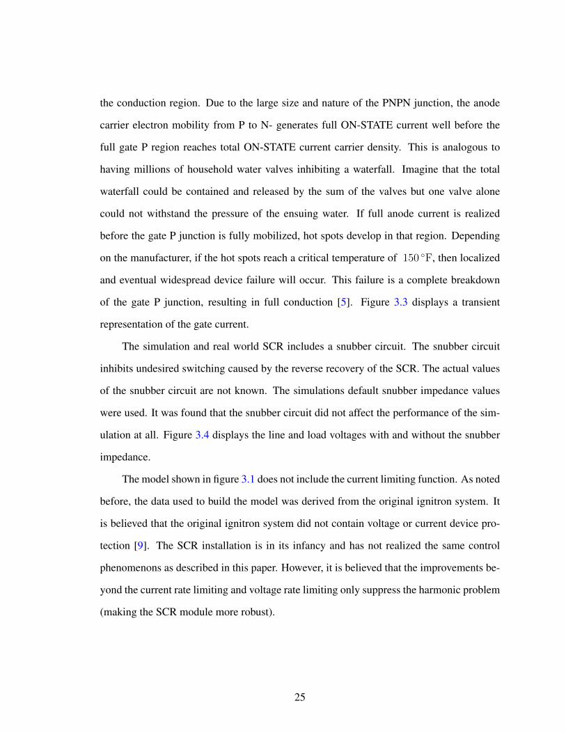
of the gate P junction, resulting in full conduction [5]. Figure 3.3 displays a transient

representation of the gate current.

The simulation and real world SCR includes a snubber circuit. The snubber circuit

inhibits undesired switching caused by the reverse recovery of the SCR. The actual values

of the snubber circuit are not known. The simulations default snubber impedance values

were used. It was found that the snubber circuit did not affect the performance of the sim-

ulation at all. Figure 3.4 displays the line and load voltages with and without the snubber

impedance.

The model shown in figure 3.1 does not include the current limiting function. As noted

before, the data used to build the model was derived from the original ignitron system. It

is believed that the original ignitron system did not contain voltage or current device pro-

tection [9]. The SCR installation is in its infancy and has not realized the same control

phenomenons as described in this paper. However, it is believed that the improvements be-

yond the current rate limiting and voltage rate limiting only suppress the harmonic problem

(making the SCR module more robust).

25

3.2 The Transformer and Total Loads

The transformer was modeled as closely as possible to the existing delta-delta substations,

the nameplate rating of the transformer, analysis performed by Krauss and associates, and

known empirical data.

Along with the current and voltage rate limiting functions, the existing system also

has a high resistance grounding system (HRG) at the secondary side of each transformer.

This addition derives a neutral voltage reference between the phases where a physical one

does not exist. Under normal (balanced load) conditions, the delta-delta transformer would

create an apparent neutral at the center of the three phase flux so that phase to ground

would be nominally 600 volts RMS. However, one phase shorting to ground causes the

neutral to “shift” from the center to the low point. The system would still operate, as each

phase to phase voltage would be identical. However, the total phase to ground voltage

would increase above 900 volts RMS. The transient switching of the SCRs could induce

over voltages in excess of 1200 volts [19]. This voltage approaches the reverse breakdown

voltage of the SCR which is approximately 1500-1800 volts. If an over voltage is sustained

for a length of time, the SCR would breakdown causing the device again to short.

The simulation enables the further understanding of the harmonic interactions between

phases. Fuzzy logic is used to characterize the system harmonic output based on varied

combinations of input phase angles from each phase. This characterization enables a rule

base to be created that identifies what phase angles are good and what phase angles should

be avoided in the control system.

26

Figure 3.2: Zero Cross Detection for SCR triggering.

27

Figure 3.3: One dimensional model representation of transient TURN ON current effects.

Figure 3.4: Graph of single phase line and load voltages with and without SCR snubberpresent.

28

Figure 3.5: Full three phase Delta-Delta transformer.

29

Introduction to Fuzzy Logic

Fuzzy logic is a method of translating fuzzy, soft phrases into crisp, quantitative values [20].

Everyday human beings use their brain to solve a problem, but the method by which the

problem is solved becomes very difficult to translate into mathematical language. Fuzzy

logic was first introduced as a way to link the non-precise descriptions of the real world

into a exact models [2]. Adjectives are used to not only describe the world we live in but

are also used to describe how we manipulate that world. An example would be giving

directions on how to do any simple task like pouring a cup of coffee. The method by which

the mind regulates the pouring of coffee is in terms like too fast, too slow, and way to slow.

Fuzzy Logic was introduced by Lotfi Zodeh in 1965, stating that “the closer one looks at a

real problem, the fuzzier its solution”[20]. The term fuzzy does not refer to something that

cannot be defined but rather a technical adjective to describe systems that have not been

previously precisely defined. Fuzzy logic is a method to precisely define the otherwise

imprecise world [2]. Much like the translation from one language to another, fuzzy logic is

a method to translate the abstract, relative world to the precise world of mathematics and

control.

30

4.1 Fuzzy Sets

In mathematics, traditional spaces are partitioned with given functions. In control theory,

a range of values can be identified by a region or space. Consider a region of all possible

values of a certain condition. Using the example of pouring coffee, all the possible values

of pouring can be bound by the region 0 to 100% pour rate. Obviously, 0% would equate to

zero pouring and 100% would equate to dumping the coffee pot completely at one time. All

the possible values in the particular context of an application are considered the universal

set U [2][1]. In classical theory, identifying a portion of this set is very binary and is

identified by specific lists or rules. For example, if the range of coffee pouring rates is

from 0-100%, a conventional set could identify all values from 35 to 75% as a medium rate

with membership of one. Fuzzy sets differ in that they have partial membership in a range.

This enables a fuzzy set to cover a non-clear boundary of values. Rather than instructing

someone to pour coffee at 50% rate, a relationship between the words pour faster can equate

to a range without clear boundaries. Figure 4.1 displays a representation of conventional

vs fuzzy set membership.

Figure 4.1: Comparison of conventional and fuzzy sets [1].

A fuzzy set in a universe of discourse U is identified by a membership function re-

ferred to as µA(x) that takes values in the interval from 0 to 1 [1]. Fuzzy sets have properties

such as compliments, unions, and intersections. Fuzzy compliments can be represented as

31

µbarA(x) = 1− µA(x)[2]. (4.1)

Figure 4.2: Complement of a fuzzy set [1].

The union of two fuzzy sets A and B are defined by a membership function

µA∪B(x) = µA(x) ∪ µB(x) = max(µA(x), µB(x))[1]. (4.2)

Figure 4.3: Union of two fuzzy sets [1].

32

The intersection of two fuzzy sets, using the product function is described by

µA∩B(x) = µA(x) ∩ µB(x) = µA(x) ∗ µB(x)[2]. (4.3)

For this thesis, the output defuzzification is performed using the product function.

Figure 4.4: Intersection of two fuzzy sets using the product method [2].

4.2 Fuzzy Partitioning

Fuzzy membership functions allow for non-definite transition between two functions. This

transition represents the ambiguous portion of fuzzy logic theory. No longer do values

have to be represented as abrupt classifications. For example, if cars are identified as red

or blue, fuzzy memberships could identify a car that is neither red or blue, but both [1]. It

is possible for a value to exist partially in a set and also in the sets compliment [2]. Figure

4.5 represents a fuzzy partitioned universe of discourse, in this case phase angle from 0 to

180◦

33

Figure 4.5: Fuzzy partitioning of a phase angle space U .

4.3 Linguistic variables

Fuzzy logic allows for the identification of fuzzy membership functions with real world ad-

jectives such as hot, less hot, more hot, cold, or really cold. These linguistic terms identify

the membership functions in common language that a mathematical (crisp) identification

can be made. In the coffee pouring example, the rate can be divided into three categories,

slow, medium, and fast. The space between 0 and 100% can then be divided into these cate-

gories and identified as such. Figure 4.6 displays the example of coffee pouring partitioned

into linquistic variables.

34

Figure 4.6: Fuzzy linguistic variables of coffee pouring rate [1].

4.4 Fuzzy Rules

Fuzzy rules identify the relationship between two universes of discourse. For example, if

a boy is very tired and not very hungry he should sleep a lot. If a boy is not very tired

but very hungry he should sleep a little. The adjectives describing how tired or hungry

the boy is identify the degrees in which the universes are partitioned. The connection of

the two conditions yields an output of additional linguistic terms that identify the universe

of amount of sleep. Rules are typically a list of if then statements that identify the input

conditions to the output conditions.

4.5 Fuzzy Control

Fuzzy logic has become increasingly popular in the last three decades. The main reason is

simply “it just works” in situations where, otherwise a conventional controller would not be

able to. The real world is full of nonlinearities, uncertain models, and behaviors that do not

hold constant with time [2]. Additionally, fuzzy controllers are more resilient to noise dis-

35

turbances than conventional PID controllers are. The effect of this is demonstrated within

this thesis. The introduction of a fuzzy harmonic mitigation controller causes nonlinearities

in the control scheme but the fuzzy proportional plus integral controller is not affected. The

fuzzy controller is comprised of four parts, fuzzification, inference evaluation, defuzzifica-

tion, and the knowledge base. Figure 4.7 displays the block diagram representation of the

components.

Figure 4.7: Block diagram of the fuzzy controller [2].

Fuzzification is the process by which the crisp input values are identified in a fuzzy

set. A crisp value can be identified in no more than two fuzzy sets. In the example of figure

4.8 the crisp value of phase angle of 45◦ is identified in two fuzzy membership functions,

low and medium. The fuzzification equates the input to being 0.2 in medium and 0.8 in low

[2].

Similarly, defuzzification is the mapping of the output response back into crisp out-

put values[2]. In control systems, the most common defuzzifcation scheme referred to as

weighted average is given by ∑U µA(x)x∑U µA(x)

. (4.4)

Using the previous example, given a range 0...180◦ an output defuzzification would be

(0.2) ∗ (0.45) + (0.8) ∗ (0.45)

(0.2 + 0.8)= 0.45 (4.5)

36

Figure 4.8: An example of fuzzification.

This example seems fairly trivial because it was assumed that the relationship between

input and output is exactly one to one. The inference engine marries the input and output

using the rule base. Consider the following rules:

If the speed of filling the cup is slow then reduce pouring slightly

If the speed of filling the cup is medium then reduce to medium pouring and,

if the speed of filling the cup is fast then reduce pouring significantly.

The figure 4.9 graphically displays how the inference engine translates the linguistics

from the rule base to the output function.

37

Figure 4.9: Min-Max method of inference to produce fuzzy sets [1].

38

Fuzzy logic is a method of translating fuzzy terms into mathematical relationships.

This chapter described the basics of fuzzy logic and fuzzy sets. Within this thesis, fuzzy

logic is used to analyze the transformer and SCR model for the purpose of identifying

the most harmful harmonics. Fuzzy logic is then used to implement two controllers, a

proportional plus integral, and a harmonic mitigation controller.

39

Fuzzy Logic Implementation

5.1 Plant Characterization using Fuzzy Logic

A simulation must be performed to observe the distortions caused by the interactions of

each SCR on a substation. The objective was to locate a region of phase angles that can

be avoided in order to reduce the total harmonic distortion of the system. For three single

phase SCRs on each substation, each one can fire from 0◦ to 180◦. Figure 5.1 gives a repre-

sentation of the simulation that was performed. For a given input phase angle combination,

there are corresponding THD and VRMS outputs. One set of inputs and outputs denote a

sample to be analyzed. Fuzzy logic is used to minimize the number of data samples taken

to characterize the system. The result of the fuzzy characterization is a region of bad phase

angles to be avoided.

From figure 5.1, the inputs and outputs are characterized into fuzzy linguistic values.

Figures 5.2 and 5.3 demonstrate the fuzzification of the inputs and outputs of the simulation

respectively. This linguistic characterization allows a range of values to be simulated and a

inference to be made about the result. For example, one simulation result may infer that if

40

Figure 5.1: Representation of the plant inputs and outputs.

the combination of inputs are “Low, Low, and Low” then the outputs are “Good”

Figure 5.2: Representation of the plant input fuzzification.

Figure 5.3: Representation of the plant output fuzzification.

41

The range of all the possible phase angles between 0◦ to 180◦ shall be considered a

universe of discourse, U [2]. Consider that there are three universes of discourse identified

by the transformer phases φA, φB, and φC and that the state of one universe affects the

other two. Without fuzzy characterization, simulations would need to be made for every

combination of phase angle for phases φA, φB, and φC . If the interactions between φA,

φB, and φC were sampled in 1◦ increments, 1803 or 5,832,000 simulations would need to

be performed. The 1◦ partitions are considered a characteristic discrimination function that

can be identified by mapping µ1◦ :→ {0, 1}[2]. To cover the entire universe of discourse,

there would need to be 180, 1◦ sets. If all the data could reasonably be collected, the

interactions between transformer phases would be identified by these 1◦ increments. In a

characteristic membership function there is no overlap. It cannot be said if an input phase

angle slightly 1◦ then it is also slightly 2◦. In fuzzy set theory, each membership function is

a collection of points within the universe. These collections, or membership functions, can

be represented in linquistic terms. For example, instead of describing the speed of a car as

50.4 mph, it can be described as fast. Degrees of fastness are held within the range of the

fuzzy membership function. For this simulation, a triangular membership function will be

used to describe the ranges of phase angles.

For the simulation in this thesis, the domain was partitioned into three membership

functions, Low, Medium, and High. For phase angles from 0◦ to 90◦, a membership func-

tion of Low was established. The word “Low” identifies all the phase angles that switch

the SCR on early in the sine wave. Similarly, the range of phase angles from 30◦ to 150◦

denotes a medium membership function, and the range 90◦ to 180◦ denotes a High mem-

bership function. Each membership function uses a triangular function with centers at 30◦,

90◦, and 150◦ for Low, Medium, and High respectively. Note that a high numerical phase

angle is equivalent to a lower applied voltage (see figure 1.1). Figure 5.4 displays the

fuzzification membership functions for the phase angle inputs.

Given these values, there are potential of 33 or 27 combinations required. Of the 27

42

Figure 5.4: Fuzzification of crisp phase angle values.

combinations, 9 can be eliminated because they do not provide any new data. The primary

phase (denoted as φA) is considered the controlling phase. Refering back to figure 1.2,

a perturbation in φB that effects φA is the same as a perturbation in phase φC . So any

combination of phase angles where φA is the same but φB and φC are interchanged will

be omitted.

Similarly, the results of the outputs will be judged by a fuzzification process. The

total resultant output from figure 5.3 will be the combination of fuzzified result of both

THD and VRMS . There will only be two membership functions for each output, Good and

Bad. In the simulation there are two outputs per phase, THD and VRMS , making a total of 6

unique outputs. Once each output is fuzzified, all 6 values will be combined. The best way

to represent this will be on a spider chart displaying all % VRMS error values and another

chart displaying all THD output values.

Figures 5.5 and 5.6 display the fuzzification membership functions for the error in

VRMS and THD respectively.

43

Figure 5.5: Fuzzification of crisp % VRMS error values.

Figure 5.6: Fuzzification of crisp THD values.

44

The % VRMS error values are calculated by comparing the output VRMS voltage of

the simulation vs the predicted or calculated RMS voltage. Purely resistive loads driven by

SCRs can be modeled by equation (5.1), where E is the RMS value of the full sine wave

and α is the SCR conduction angle [21]. Figure 5.7 shows a comparison of the calculated

VRMS voltage and the simulated VRMS voltage.

VRMS = E ∗√

1 − α

π− sin(2α)

2π(5.1)

Figure 5.7: VRMS vs phase α with varied loads.

Additionally, the total harmonic distortion of the supply transformer, reflects the im-

pact of the SCR on the delta transformer and adjacent single phase SCRs. According to

the IEEE 519 standard, total harmonic distortion is given by the square root of the sum

of squares of the voltage magnitude of the harmonic content, divided by the square of the

45

magnitude of the fundamental voltage equation (5.2) [3][14].

PLANT =

√√√√ n∑h=2

Vh2

V1∗ 100% (5.2)

In these values, error from expected VRMS vs simulated VRMS was compared. Figure

5.8 displays the % error from the calculated VRMS at each combination. A radar chart

is best used to visualize the interactions between phases. It can be seen that the primary

phase has the worst result vs the expected at the HMM, HHH, and HLM combinations

respectively. The HMM combination is so extreme that the expected voltage is suppressed

to 0. This is due to the harmonic interactions of two other phases at the worst harmonic

extreme. It is interesting to see that the interactions of phase C are affected by both MLH

and MMH combinations.

Figure 5.8: % VRMS error of each transformer phase vs SCR phase angle combinations.

46

Figure 5.9 displays the THD radar chart of each phase of the substation. It can be

observed how each phase is affected by the each other. It can be seen in figure 5.8 and

figure 5.9 that all three phases align in both voltage drop and distortion when they are

balanced.

Another viewpoint is given in figure 5.10 which displays the standard deviation of

the error of each phase. This chart explains the significance of balanced three phases vs

unbalanced.

Figure 5.9: THD of each each transformer phase vs SCR phase angle combinations.

The simulation demonstrated two things. First, if all three phases act in harmony (are

balanced) then the distortion is balanced, i.e., the overall error from expected RMS voltage

to actual may be high but every phase has the same, predictable, output. The balanced loads

cause the distortion to be “linear” in effect, allowing for conventional control methods to

work. In fact, one of the facilities used in this case study routinely runs all three phases in

47

Figure 5.10: Standard deviation of %VRMS error of each transformer phase vs SCR phaseangle combinations.

a balanced configuration without control problems.

It seems that the control issues occur when the distortion of the unbalanced loads

drastically suppresses the output of one of the three phases. The particular example demon-

strated in figure 5.8 shows that certain combinations yield total suppression of an output.

To a classical PI controller, this can be extremely problematic. If the controller is expecting

a certain output to reduce error and does not receive it consistently, high integration gain

could cause the controller to go unstable. It was also observed that the most problematic

combinations occur when one or two phases are in the median range of phase angles. Table

5.1 displays the resultant combinations that yield either a bad harmonic interaction or a

good one. Essentially, any interactions with a medium phase angle are considered harmful.

To determine a relative range of medium phase angles that need to be isolated, further

simulations were carried out by incrementing the phase angle for only one transformer leg

48

φA φB φC ResultL L L GOODL L H GOODL H H GOODH L L GOODH L H GOODH H H GOODH M H BADL L M BADL M M BADL M H BADM L L BADM L M BADM L H BADM M M BADM M H BADM H H BADH L M BADH M M BAD

Table 5.1: Combinations of fuzzification centers for rule generation.

while keeping the other two legs at zero. This experiment demonstrates the overall effect

of just one phase’s interaction with the substation.

Figure 5.11 displays the percent harmonic distortion effect on the substation phase in

relation to the load. As the single phase load increases, the distortion due to the switching

power also increases. Figure 5.12 displays the effect of one phase switching at 10 degree

increments.

The single phase representation of THD vs phase angle displays a bell curve around

the middle or medium phase angles. A definitive band of middle phase angles cannot be

isolated completely but the range from 60 to 120 degrees appears to produce the most total

harmonic distortion.

In the proposed solution, each single phase SCR controller will contain a control loop

that maintains the current control profile. The controller will also contain a harmonic mit-

igation controller that will simply eliminate the harmful band of harmonics. The profile

49

Figure 5.11: THD vs phase α with varied loads.

controller is designed as a fuzzy PI controller to improve performance over a conventional

PI controller. The harmonic mitigation controller is a fuzzy proportional controller that has

a very unique rule base centered around eliminating the identified region of harmonics.

50

Figure 5.12: THD of each φ vs phase α with a single phase 400KW load.

5.2 The PI Controller Implementation

5.2.1 The Radiant Heat System Plant

An additional simulation was created to model the equivalent RMS characteristic of the

plant. This model does not incorporate the transformer and SCR interactions but models

the equivalent RMS voltage that the SCR would produce. The objective of this model is to

show a typical heat system performance and show that the harmonic mitigation controller

does not affect that performance. The first step to model the harmonic mitigation controller

is to establish a baseline simulation of which a conventional controller operates. This

controller will demonstrate the characteristic response of the entire radiant heating system.

Most of the discussion concerning the system input has concentrated on the phase

51

angle of the SCR. External to the SCR itself, the radiant heating controller inputs a drive

signal to the SCR. The SCR controller contains a control loop that ensures that a propor-

tional drive input equals a proportional VRMS out regardless of the magnitude of the load.

The relationship between input drive signal and output VRMS is a linear relationship with

a slope equal to one. This transfer function is controlled by the SCR controller. As stated

earlier in equation (5.1), a direct correlation between drive and VRMS can be made with

resultant output much like figure 5.7. An alignment procedure is performed on the SCR

to ensure the slope of the controller input vs output is always equal to one. Figure 5.13

displays the representative SCR inner loop.

Figure 5.13: Representative SCR inner loop.

Phase angle, as discussed earlier, is not directly realized in our controller, only the

drive that is requested. The SCR has an internal loop that applies an additional amount of

phase, depending on the load, to achieve the drive requested. The controller must translate

what phase angles to avoid to a range of drive output. This translation is a one to one scale

only if the controller updates control loop at least once per cycle, driving the output to a

new phase before the inner SCR loop can compensate.

This result suggests that the controller update frequency must be in phase with the

sine cycle, meaning a linear multiple of 60 Hz. A controller update rate much greater than

60 Hz is not necessary. The controller cycle must be a linear multiple of 60 Hz in order to

intercept the drive and determine an appropriate phase angle.

Typical heat transfer systems have a very low bandwidth on the order of 1 to .1 hertz

with respect to temperature. However, this depends highly on the test article, the proximity

of the heating device, and the rate at which the device must be heated. Most heating pro-

52

files are a ramp function in nature from the ambient temperature to a known temperature

followed by a hold or “soak” time and then a ramp down period. Although not correlated

fully, a characteristic second order equation was imperially derived from test data and past

modeling data. This transfer function is in no way representative of an actual heat transfer

system but emulates the behaviors sufficiently enough to demonstrate a fuzzy logic con-

troller. An excel sheet that emulated the heat transfer behaviors of two re-radiating plates

was used to model the equation. Figure 5.14 demonstrates a typical heat transfer setup

where the top plate (the heater) radiates energy to the bottom plate (the test article). The

controller adjusts the drive signal in order to follow a prescribed profile on the bottom

plate[22]. The excel macro incorporates a difference equation that inputs the heat transfer

parameters and outputs the temperature vs time resultant curve. Figure 5.15 displays the

resultant curve implementing a step function in the heater array from 0 to full drive. Full

drive is considered to be 5500 ◦F .

Figure 5.14: Representative heat transfer from heating element to test article.

In addition to this data, test data was analyzed and modeled as well. From the test

data and the heat transfer model, the characteristic equation (5.3) was formed. This is

considered a type 0 system. The system has a bandwidth of 0.017 Hz. Much slower than

the required bandwidth of the SCRs. In fact, typical heat profiles are no greater than 30 to

60 degrees per second.

53

Figure 5.15: Representative heat transfer from heating element to test article resultantgraph.

0.025

s2 + 0.85s+ 0.025(5.3)

It is to be noted that the system damping ratio is greater than 1. This causes the system

to be over-damped, and on its own it will not overshoot. This system is incorporated into

an open loop system detailed in figure 5.16 and the sub function containing the equations

for RMS voltage, power, and surface temperature are shown in figure 5.17. The inner sub

function accepts a normalized drive signal and translates it to an equivalent phase angle,

which is calculated as RMS voltage and power. Figure 5.18 shows the results of SCR %

drive vs Graphite element temperature. Figure 5.19 displays the resultant output voltage

and power vs drive signal.

54

Figure 5.16: Open loop plant with SCR, heater, and simulated plant.

55

Figure 5.17: Representative SCR inner model.

56

Figure 5.18: Drive% vs. Telement(◦F ).

57

Figure 5.19: VRMS and PRMS with respect to drive %.

58

5.2.2 The Initial Linear Controller

The classical controller design is the first step in the fuzzy PI controller design as the

same gains are used for both. The classical controller was designed for no more than 10%

overshoot and zero steady state error to a step input. These design constraints yield better

performance to a ramp input. The desire is to achieve < 1% overshoot and < 0.2% steady

state error to a ramp input. It is a typical practice to tune heat control systems using a small

step input, ensuring better response to a ramp input. As stated earlier, the SCR internal

controller is assumed to be completely linear with a slope of 1. Therefore the control loop

has the fundamental model shown in figure 5.20

Figure 5.20: Simulink model of the representative analog control system

The plant,given by equation (5.3), is a type 0 system. For steady state error to be 0, an

integrating action must be added, increasing the type from 0 to 1 [2]. The first design step

is to find the proportional gain Kp. Figure 5.21 displays the root locus of the open loop

transfer function with the PI controller. AssumingKi/Kp is very close to zero (or<< 0.8).

Assume Ki/Kp = .04. The forward path transfer function is give by equation (5.4).

plant =0.025 ∗Kp ∗ (s+ Ki

Kp)

s(s2 + 0.85s+ 0.025)(5.4)

By assuming that Ki/Kp is very close to zero, the forward path transfer function can be

59

Figure 5.21: Root locus of the open loop transfer function

reduced to equation (5.5).

plant =0.025 ∗Kp

(s2 + 0.85s+ 0.025)(5.5)

Obtaining the closed loop transfer function yields equation (5.6).

plant =0.025 ∗Kp

(s2 + 0.85s+ (0.025 ∗ 1 +Kp))(5.6)

From a design requirement of less than 10% overshoot the damping ratio of the prototype

60

second order system, ζ can be found using equation (5.7) [23].

100e−πζ√1−ζ2 = 5% (5.7)

ζ =

√n

1 + n(5.8)

when

n =

(ln(OverShoot)

π

)2

(5.9)

61

From equations (5.9) and (5.8), ζ was found to be 0.5912, which gave an overshoot

of 9.99%. Using Kp = ω2n

0.025− 1 where ωn = 0.85

2∗ζ , Kp was found to be 19.67. Since

Ki/Kp = .04, Ki was found to be 0.7.

Figure 5.22 displays the entire continuous model that is used for the fuzzy logic con-

troller design. Figure 5.23 displays the response of the closed loop system in figure 5.22 to

a ramp signal to 50% of full temperature or 2750◦ F .

62

Figure 5.22: Simulink model of the analog control system

63

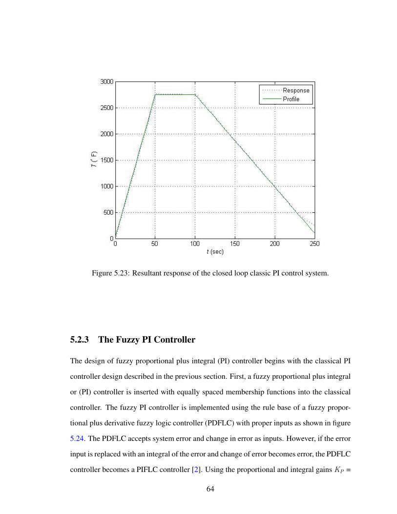
Figure 5.23: Resultant response of the closed loop classic PI control system.

5.2.3 The Fuzzy PI Controller

The design of fuzzy proportional plus integral (PI) controller begins with the classical PI

controller design described in the previous section. First, a fuzzy proportional plus integral

or (PI) controller is inserted with equally spaced membership functions into the classical

controller. The fuzzy PI controller is implemented using the rule base of a fuzzy propor-

tional plus derivative fuzzy logic controller (PDFLC) with proper inputs as shown in figure

5.24. The PDFLC accepts system error and change in error as inputs. However, if the error

input is replaced with an integral of the error and change of error becomes error, the PDFLC

controller becomes a PIFLC controller [2]. Using the proportional and integral gains KP =

64

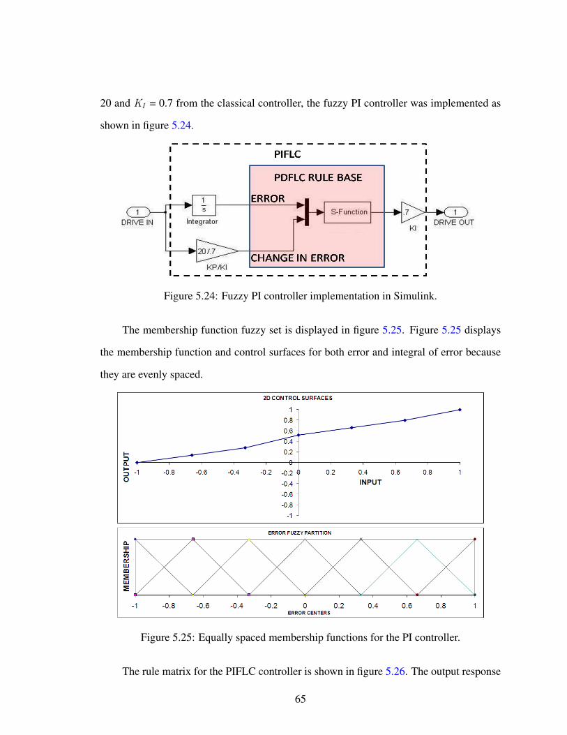
20 and KI = 0.7 from the classical controller, the fuzzy PI controller was implemented as

shown in figure 5.24.

Figure 5.24: Fuzzy PI controller implementation in Simulink.

The membership function fuzzy set is displayed in figure 5.25. Figure 5.25 displays

the membership function and control surfaces for both error and integral of error because

they are evenly spaced.

Figure 5.25: Equally spaced membership functions for the PI controller.

The rule matrix for the PIFLC controller is shown in figure 5.26. The output response

65

is displayed in figure 5.27. This graph is zoomed in to view the steady state and overshoot

of the response. The overshoot is 1.8% and the steady state error is .001%. The errors

are within tolerances without changing the fuzzy controller membership functions at all.

Typically, the decent ramp is not as critical due to the natural cooling of the article.

Figure 5.26: Rule Base for the standard Fuzzy Proportional Plus Integral Controller.

Figure 5.27: Response of the evenly spaced Fuzzy Logic PI controller.

66

Figure 5.28: The phase angle output of the evenly spaced Fuzzy PI controller.

67

The next step is to use the fuzzy membership functions to improve the performance of

the system. At small amounts of error, the controller does not provide enough drive to reach

the set point. By narrowing the inner membership function centers, more drive is available

at lower error levels. Figure 5.29 displays the resultant output of the fuzzy controller with

the error membership functions (figure 5.30) modified from evenly spaced.

Figure 5.29: Modified Fuzzy PI controller System Response.

The new overshoot is 0.34% and the steady state error is 0.12%. The small sacrifice

for steady state error is acceptable to gain an under 1% overshoot. The advantages to the

fuzzy controller would be more significantly realized on a plant that has an initial delay in

the system. More research would need to be performed to emulate the delay in heat transfer

since this is not a constant phenomenon. Next, the fuzzy harmonic mitigation controller

will be included in the system. This will eliminate harmful harmonics but not disturb the

present control performance.

68

Figure 5.30: Control Surface for the error signal.

5.3 The Fuzzy Harmonic Reduction Controller

To implement harmonic mitigation, a harmonic fuzzy controller will be incorporated in the

system. This can be referred to as the Fuzzy PH controller for proportional harmonic since

the controller is nothing more than a proportional fuzzy logic controller with a unique rule

base. Figure 5.31 displays the phase angle output with the classic control implemented

only. Notice the spike that resides in the region of 90◦ to 110◦ phase angle (figure 5.32).

This will be the region where the fuzzy harmonic controller will take over, by either in-

creasing or decreasing the phase angle to avoid this region.

69

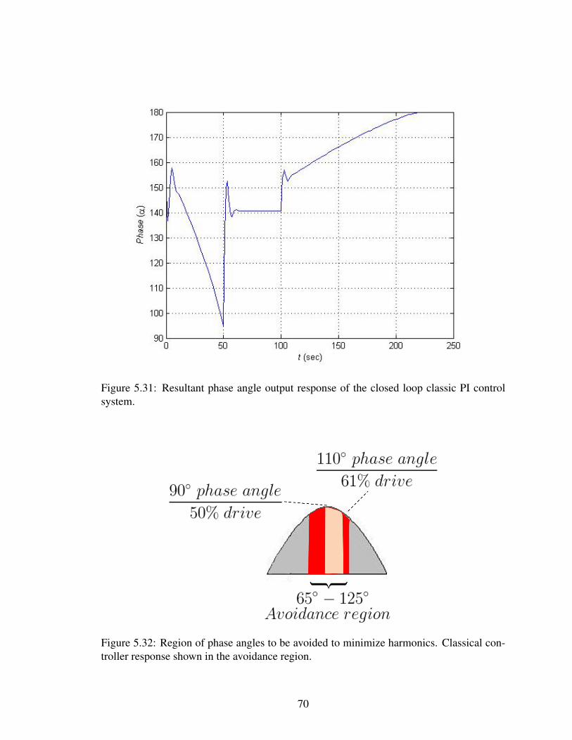
Figure 5.31: Resultant phase angle output response of the closed loop classic PI controlsystem.

Figure 5.32: Region of phase angles to be avoided to minimize harmonics. Classical con-troller response shown in the avoidance region.

70

The more phases that are eliminated from the drive space, the longer it will take for

the controller to resolve the requested drive (provided no instability occurs). Consider that

a test system needs an equivalent RMS voltage of 300 volts maintained on the heater to

provide the temperature transfer required. A “Middle” phase angle is required to maintain

the total RMS voltage of 300V. In order to provide a 300V RMS, a phase angle of 90 de-

grees would be required. If the ‘Medium” range extended from 60 degrees to 120 degrees,

the controller would need to either provide too much power or too little. Considering that

heat transfer is a low bandwidth process, if the controller provided too much power for a

very short time, and then too little power for the rest, the average output over time would

still yield the same result. This would only be feasible if the system bandwidth could ac-

commodate a delay in achieving the desired set point. Since every test is different, range

of Medium or bad phase angles can become wider or narrower depending on the trade off

of harmonic distortion vs bandwidth. To prove that the elimination of harmonics is feasi-

ble, the controller implementation will eliminate the range from approximately 55 to 125

degrees phase angle.

One of the challenges with radiant heat testing is the inability to provide negative

drive. Essentially, whatever power is provided to the test article cannot be taken back. The

controller has to rely on the constant cooling rate of either ambient temperature or a cooling

mechanism such as forced air convection. Very few test systems provide a mechanism for

active cooling. So for a fuzzy controller, (NB) would be considered 0 drive. The “stronger”

weighting that is put on the negative membership functions, the more dwell time will be

spent at 0 drive, depending on the natural transfer of heat energy out of the test article.

In the routine that translates drive into VRMS , a single input, single output fuzzy con-

troller is implemented. The controller is implemented using the proportional fuzzy con-

troller [2]. Similar to the PI controller discussed in the previous section, this controller

implements triangle membership functions. The range is scaled however from [-1:1] to

[0:1]. This corresponds to 0-100% drive. The rule base creates a digital switch in the con-

71

troller that nearly bypasses regions of high harmonics. In fuzzy control, the combination

of two fuzzy membership functions must always equal one. Therefore, the centers of two

membership functions cannot be equal. For the harmonic mitigation controller, the objec-

tive is to “skip” the harmful harmonics. Figures 5.33, 5.35, and 5.36 display the control

surface, input, and output membership functions respectively. Notice that the membership

functions for both the input and output have areas that the membership function centers

appear to be touching.

Figure 5.33: Control surface for harmonic mitigation controller.

Figure 5.34 shows the control surface from 29.98% input drive to 30.05% input drive.

It can be seen from this figure that the membership function centers are not touching, but

very nearly. Between 30-30.01% input drive (or an equivalent 54 − 54.09◦ phase angle)

the output will be in the harmful phase angle region. The objective is to minimize the time

the controller spends in the area of harmful harmonics. Essentially, the gain in the region

of disinterest is extremely high, forcing the controller to either increase to a higher output

value or decrease dramatically. Basically, the primary rule was to avoid all frequencies

that prove to be harmful for harmonics. Eliminating these frequencies creates a void in

the continuous control, thereby inducing a hybrid pulse width modulation control. A seven

membership fuzzy controller was used to create a near stair step approach to the input vs

output of the controller.

72

Figure 5.34: Close up of the harmful harmonic region in the control surface for harmonicmitigation controller.

Figure 5.35: Error membership function for the harmonic mitigation controller.

Figure 5.36: Output membership function for the harmonic mitigation controller.

73

Figure 5.37 displays the full system with the additional harmonic mitigation controller

added. The fuzzy PI controller input and output centers did not change at all.

As error increases in any of the flat regions, the relative duty cycle increases until the

error is too great and the next stair step is achieved. Figure 5.38 displays the comparison

of phase angle drive with and without the controller. Notice the void of frequencies used in

with the Harmonic Reduction controller. Figure 5.39 displays just the harmonic reduction

controller as a line plot to visualize the hybrid pulse width modulation. The stair step

approach avoids having too much time in one region, a trade off is obviously made in the

magnitude of error vs the maximum duty cycle of the hybrid controller steps. Figure 5.41

displays a close up look of figure 5.38. The closeup allows a better view of the duty cycle

of the switching. The duty cycle of the switching is well within the 60 Hz update rate

required for the SCR cycle.

74

Figure 5.37: Complete system with harmonic mitigation fuzzy Controller.

75

Figure 5.38: Resultant phase control output with and without harmonic reduction con-troller.

Figure 5.39: Resultant phase control output with harmonic reduction controller.

76

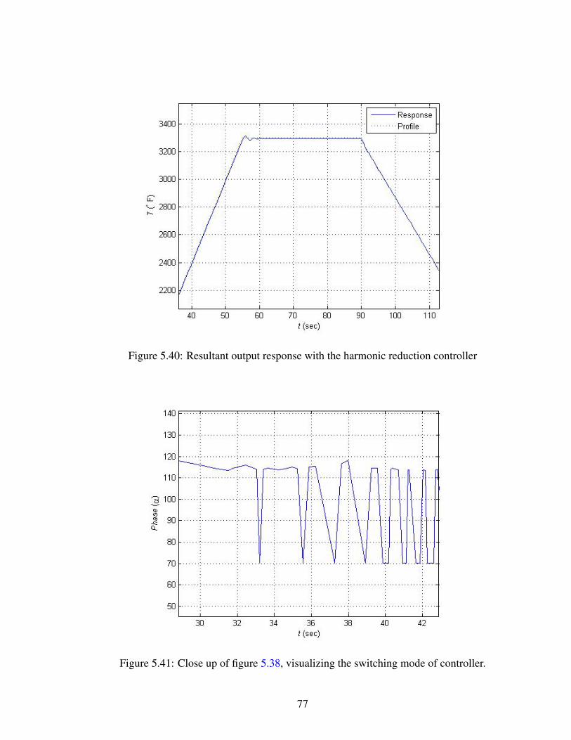
Figure 5.40: Resultant output response with the harmonic reduction controller

Figure 5.41: Close up of figure 5.38, visualizing the switching mode of controller.

77

The steady state error is 0.003% and the overshoot is 0.45%. Therefore, the harmonic

mitigation controller eliminated the use of phase angles that are known to cause harmonic

distortion and still maintained control of the plant. This is achieved without any hardware

added to the system.

78

Conclusions

Harmonic disturbances in power systems may be common, but solutions are unique in the

fact that each industrial power system is different. Many industrial plants spend millions of

dollars and perform lengthy analysis to eliminate harmonics that cause machinery to fail,

computers to crash, and power service charges to increase. Most solutions use hardware

in the form of large capacitor banks or switching resistors to cancel out these harmful

harmonics, all of which continue to waste additional energy.

An approach to eliminating harmonics without adding additional hardware is pre-

sented in this paper. The applications can extend to any high power transfer mechanism

where the control loop is modifiable. This thesis presented a method of simulating the tran-

sient behavior of power plant in Matlab SymPowerSystems. The plant consisted of single

phase, silicon controlled rectifiers (SCR) fed by an unbalanced delta-delta transformer. It

could be observed in the simulations that the harmonic disturbances were so problematic

in this design case that an entire phase of the transformer would be suppressed to zero. The

classical control system used in the facility would sometimes not be able to compensate for

the harmonic disturbances and cause the system to go out of control.

There are many methods to analyze a problem to come to a conclusion. Unique to this

thesis was the use of fuzzy logic as a method to characterize a system. The system was

79

characterized by partitioning the input parameters and output parameters. These partitions

were combined to generate analytical conclusions about the plant harmonic problem. It

was found that if an SCR controller could eliminate use of a region of phase angles, the

total harmonic distortion (THD) of the power plant would be reduced without the addition

of any hardware.

Implementing this control scheme identified the non-linearity of the plant to be con-

trolled. The best method to control a non-linear plant was to use fuzzy logic. It was shown

that the performance of the plant even before eliminating the harmful harmonics could be

improved by replacing the classical proportional plus integral (PI) controller with a fuzzy

logic PI controller. An additional controller was then added to reduce the region of SCR

phase angles that caused the most harmful harmonics. This controller again was imple-

mented using fuzzy logic. The power of fuzzy logic was the ability to have a control space

that in linear regions that produce little harmonic disturbance and non-linear regions that

a cause disturbance. The harmonic controller elimated harmful harmonics from the plant

without the addition of hardware and did not affect plant control.

Future work could incorporate the fuzzy logic characterization engine into the har-

monic distortion controller. By monitoring a range of BAD phase angles, the range of

phase angles to avoid could be automatically adjusted. This would require monitoring the

VRMS and the THD for each phase and adjust the phase band of the harmonic controller

based on the region with the most harmonic disturbance.

80

Bibliography

[1] A. P. Khatra, “IMPLEMENTATION OF A MULTI-LAYERED FUZZY CON-

TROLLER ON AN FPGA,” Master’s thesis, Wright State University, Dayton, Ohio,

July 2006.

[2] “Fuzzy logic control summer 2000,” notes for EE419. [Online]. Available:

kuldip.rattan@wright.edu

[3] Unknown, “Ieee recommended practices and requirements for harmonic control in

electrical power systems,” IEEE Std 519-1992, pp. –, Apr 1993.

[4] P. Hammond, “Balancing device stresses by fundamental cancellation,” Industry Ap-

plications, IEEE Transactions on, vol. 29, no. 2, pp. 369–374, Mar/Apr 1993.

[5] U. Mohan, Robbins, Power Electronics: Converters, Applications, and Design. Wi-

ley, 1989.

[6] B. G. Liptak, Instrumentation in the processing industries. Bela G. Liptak, editor,

[3rd ed.] ed. CRC Press, 1995.

81

[7] T. Skvarenina, S. Pekarek, O. Wasynczuk, P. Krause, R. Thibodeaux, and J. Weimer,

“Simulation of a switched reluctance, more electric aircraft power system using

a graphical user interface,” in Energy Conversion Engineering Conference, 1997.

IECEC-97., Proceedings of the 32nd Intersociety, vol. 1, Jul-1 Aug 1997, pp. 580–

584 vol.1.

[8] R. Fields, “Flight vehicle thermal testing with infrared lamps,” NASA Dryden

Flight Research Facility, Tech. Rep., 1992. [Online]. Available: http://www.nasa.

gov/centers/dryden/pdf/88257main H-1779.pdf

[9] E. Schiff, “Study of heating methods for structural testing ¿ 3000 deg f,” Wpafb, Tech.

Rep., 1965.

[10] G. Chen, 2.58J Radiative Transfer, License: Creative Commons BY-NC-SA,

(Massachusetts Institute of Technology: MIT OpenCourseWare) Std., Spring 2006.

[Online]. Available: http://ocw.mit.edu

[11] K. Leger, “Modular resistance heater assembly,” USA Patent 4 927 994, 1990.

[Online]. Available: http://www.patentstorm.us/patents/pdfs/patent id/4927994.html

[12] R. Walling, R. Hartana, and W. Ros, “Self-generated overvoltages due to open-

phasing of ungrounded-wye delta transformer banks,” Power Delivery, IEEE Trans-

actions on, vol. 10, no. 1, pp. 526–533, Jan 1995.

[13] M. H. Rashid, Power Electronics Handbook, Second Edition: Devices, Circuits and

Applications (Engineering), 2nd ed. Academic Press, 11 2006. [Online]. Available:

http://amazon.com/o/ASIN/0120884798/

[14] P. Hammond, “A harmonic filter installation to reduce voltage distortion from static

power converters,” Industry Applications, IEEE Transactions on, vol. 24, no. 1, pp.

53–58, Jan/Feb 1988.

82

[15] M. H. RASHID, Power Electronics Handbook. ACADEMIC PRESS, 2001.

[16] M. Bech, F. Blaabjerg, and J. Pedersen, “Random modulation techniques with fixed

switching frequency for three-phase power converters,” Power Electronics, IEEE

Transactions on, vol. 15, no. 4, pp. 753–761, Jul 2000.

[17] M. E. M. Benghanem, A. Draou, “Fuzzy logic pi control applied to static

var compensator using n.p.c inverter topology.” [Online]. Available: http:

//www.emo.org.tr/ekler/292b3e9629fee6b ek.pdf

[18] B. Noyes, “The variation in the resistance of carbon and graphite with temperature,”

Phys. Rev., vol. 24, no. 2, pp. 190–199, Aug 1924.

[19] R. Beltz, I. Peacock, and W. Vilcheck, “High-resistance ground retrofits in pulp and

paper mills,” Industry Applications Magazine, IEEE, vol. 7, no. 2, pp. 19–27, Mar/Apr

2001.

[20] L. Reznik and L. Reznik, Fuzzy Controllers: How to Design Them, how They Work.

Newton, MA, USA: Butterworth-Heinemann, 1997.

[21] C. C. Inc., “Tungsten lamp characteristics,” application note.

[22] L. BYRD, “Heat transfer excel macro,” 2004.

[23] B. Kuo, Automatic Control Systems, Seventh Edition. Prentice-Hall, 1995.

83

Appendix A: Matlab Code

ruledefine.m

\label{RuleCode}

clear all

clc

ot=[-1 -.66 -.33 0 .33 .66 1];

centers2=[-1 -.66 -.33 0 .33 .66 1];%error

centers1=[-1 -.66 -.33 0 .33 .66 1];%integral error

%Fuzzy harmonic Controller rule base

centers = [0 0.15 0.35 0.56 0.68 0.8 1];

rule_vector= [0 0.15 0.35 0.56 0.68 0.8 1]’;

NB=ot(1);

NM=ot(2);

NS=ot(3);

Z=ot(4);

PS=ot(5);

PM=ot(6);

PB=ot(7);

rule_matrix=

[[NB NB NB NB NM NS Z];

[NB NB NB NM NS Z PS];

84

[NB NB NM NS Z PS PM];

[NB NM NS Z PS PM PB];

[NM NS Z PS PM PB PB];

[NS Z PS PM PB PB PB];

[Z PS PM PB PB PB PB]]

zfunc.m

%function y = zfunc(x,CP,a)

%Matt Clark

function y = zfunc(x,cp,a)

if x <= cp

y = 1;

elseif x < a

y = (a-x)/(a-cp);

else

y = 0;

end

fuzzify.m

%function U = fuzzify(x,Centers)

%Matt Clark

function U = fuzzify(x,Centers);

Len=length(Centers);

U=zeros(1,Len);

if x<=Centers(2)

U(1)=zfunc(x,Centers(1),Centers(2));

U(2)=triangle(x,Centers(2),[Centers(1) Centers(3)]);

return

elseif x>=Centers(Len-1)

U(Len)=sfunc(x,Centers(Len),Centers(Len-1));

85

U(Len-1)=triangle(x,Centers(Len-1),[Centers(Len-2) Centers(Len)]);

return

end

for i=2:(Len-2)

if x>=Centers(i)

U(i)=triangle(x,Centers(i),[Centers(i-1) Centers(i+1)]);

U(i+1)=triangle(x,Centers(i+1),[Centers(i) Centers(i+2)]);

end

end

sfunc.m

%function y = sfunc(x,CP,a)

%Matt Clark

function y = sfunc(x,cp,a)

if x <= a

y = 0;

elseif x < cp

y = (x-a)/(cp-a);

else

y = 1;

end

pflc.m

%function Y = pflc(x,Centers,Rule_Vector)

%Matt Clark

%DESCRIPTION

function Y = pflc(x,Centers,Rule_Vector);

e=fuzzify(x,Centers);

86

parts=find(e);

[o,p]=size(parts);

R=Rule_Vector;

if p==1

R=R(parts,1);

e=e(1,parts);

else

R=[R(parts(1),1);R(parts(2),1)];

e=[e(1,parts(1)) e(1,parts(2))];

end

Y=e*R;

pdflc.m

%function Y = pdflc(e,ce,Centers_e,Centers_ce,Rule_Matrix)

%Matt Clark

%DESCRIPTION

function Y = pdflc(Xe,Xce,centers1,centers2,rule_matrix);

e=fuzzify(Xe,centers1);

ce=fuzzify(Xce,centers2);

Y=e*rule_matrix*(ce.’);

87