The Handbook of Trading: Strategies for Navigating and ......Delaware Derivative Action 171 Edward...
497
Transcript of The Handbook of Trading: Strategies for Navigating and ......Delaware Derivative Action 171 Edward...


The
HANDBOOKof
TRADING

Other McGraw-Hill Books Edited by Greg N. Gregoriou
The Credit Derivatives Handbook: Global Perspectives, Innovations, and MarketDrivers (2008, with Paul U. Ali)
The Handbook of Credit Portfolio Management (2008, with Christian Hoppe)
The Risk Modeling Evaluation Handbook (2010, with Christian Hoppe andCarsten S. Wehn)
The VaR Implementation Handbook (2009)
The VaR Modeling Handbook: Practical Applications in Alternative Investing,Banking, Insurance, and Portfolio Management (2009)

The
HANDBOOKof
TRADING
New York Chicago San FranciscoLisbon London Madrid Mexico City
Milan New Delhi San Juan SeoulSingapore Sydney Toronto
STRATEGIES FOR NAVIGATING
AND PROFITING FROM CURRENCY,
BOND, AND STOCK MARKETS
Greg N. GregoriouEditor

Copyright © 2010 by The McGraw-Hill Companies, Inc. All rights reserved. Except as permitted under the United States Copyright Act of 1976, no part of this publication may be reproduced or distributed in any form or by any means, or stored in a database or retrieval system, without the prior written permission of the publisher.
ISBN: 978-0-07-174354-9
MHID: 0-07-174354-5
The material in this eBook also appears in the print version of this title: ISBN: 978-0-07-174353-2, MHID: 0-07-174353-7.
All trademarks are trademarks of their respective owners. Rather than put a trademark symbol after every occurrence of a trademarked name, we use names in an editorial fashion only, and to the benefi t of the trademark owner, with no intention of infringement of the trademark. Where such designations appear in this book, they have been printed with initial caps.
McGraw-Hill eBooks are available at special quantity discounts to use as premiums and sales promotions, or for use in corporate training programs. To contact a representative please e-mail us at [email protected].
This publication is designed to provide accurate and authoritative information in regard to the subject matter covered. It is sold with the understanding that neither the author nor the publisher is engaged in rendering legal, accounting, futures/securities trading, or other professional service. If legal advice or other expert assistance is required, the services of a competent professional person should be sought. —From a Declaration of Principles jointly adopted by a Committee of the American Bar Association and a Committee of Publishers
TERMS OF USE
This is a copyrighted work and The McGraw-Hill Companies, Inc. (“McGrawHill”) and its licensors reserve all rights in and to the work. Use of this work is subject to these terms. Except as permitted under the Copyright Act of 1976 and the right to store and retrieve one copy of the work, you may not decompile, disassemble, reverse engineer, reproduce, modify, create derivative works based upon, transmit, distribute, disseminate, sell, publish or sublicense the work or any part of it without McGraw-Hill’s prior consent. You may use the work for your own noncommercial and personal use; any other use of the work is strictly prohibited. Your right to use the work may be terminated if you fail to comply with these terms.
THE WORK IS PROVIDED “AS IS.” McGRAW-HILL AND ITS LICENSORS MAKE NO GUARANTEES OR WARRANTIES AS TO THE ACCURACY, ADEQUACY OR COMPLETE-NESS OF OR RESULTS TO BE OBTAINED FROM USING THE WORK, INCLUDING ANY INFORMATION THAT CAN BE ACCESSED THROUGH THE WORK VIA HYPERLINK OR OTHERWISE, AND EXPRESSLY DISCLAIM ANY WARRANTY, EXPRESS OR IMPLIED, INCLUD-ING BUT NOT LIMITED TO IMPLIED WARRANTIES OF MERCHANTABILITY OR FITNESS FOR A PARTICULAR PURPOSE. McGraw-Hill and its licensors do not warrant or guarantee that the functions contained in the work will meet your requirements or that its operation will be uninterrupted or error free. Neither McGraw-Hill nor its licensors shall be liable to you or anyone else for any inaccuracy, error or omission, regardless of cause, in the work or for any damages resulting therefrom. McGraw-Hill has no responsibility for the content of any information accessed through the work. Under no circumstances shall McGraw-Hill and/or its licensors be liable for any indirect, incidental, special, punitive, consequential or similar damages that result from the use of or inability to use the work, even if any of them has been advised of the possibility of such damages. This limitation of liability shall apply to any claim or cause whatsoever whether such claim or cause arises in contract, tort or otherwise.

CONTENTS
EDITOR xvii
CONTRIBUTORS xix
ACKNOWLEDGMENTS xxxiii
PA RT I EXECUTION AND MOMENTUM TR ADING 1
C H A P T E R 1 Performance Leakage and ValueDiscounts on the TorontoStock Exchange 3
Lawrence Kryzanowski and Skander LazrakAbstract 3Introduction 4Sample and Data 5Measures of Performance Leakage and Value Discounts 5Empirical Estimates for the TSX 7Conclusion 18Acknowledgments 18References 19Notes 20
C H A P T E R 2 Informed Trading in ParallelAuction and Dealer Markets: The Case of the London Stock Exchange 23
Pankaj K. Jain, Christine Jiang, Thomas H. McInish, and Nareerat Taechapiroontong
Abstract 23Introduction 23Trading Systems and Venues 24Institutional Background, Data, and Methodology 27
v

Empirical Results 30Conclusion 35Acknowledgments 36References 36Notes 38
C H A P T E R 3 Momentum Trading for thePrivate Investor 39
Alexander Molchanov and Philip A. StorkAbstract 39Introduction 39Data 40Momentum Trading Results 41Robustness Tests 45Trading with a Volume Filter 47Private Investor Trading 49Conclusion 50Acknowledgments 51References 51Notes 52
C H A P T E R 4 Trading in Turbulent Markets: Does Momentum Work? 53
Tim A. Herberger and Daniel M. KohlertAbstract 53Introduction 53Literature Review 54Data and Methodology 55Results 57Conclusion 62References 63Notes 65
C H A P T E R 5 The Financial Futures Momentum 67
Juan Ayora and Hipòlit TorróAbstract 67Introduction 67Literature Review 68
vi contents
Data 69Methodology and Results 69Conclusion 77Acknowledgments 79References 79Notes 80
C H A P T E R 6 Order Placement Strategies inDifferent Market Structures: A Primer 83
Giovanni PetrellaAbstract 83Introduction 83Costs and Benefits of Limit Order Trading 84Trading in a Continuous Order-Driven Market 86Trading in a Call Auction 89Conclusion 91References 92
PA RT II TECHNICAL TR ADING 95
C H A P T E R 7 Profitability of Technical Trading Rules in an EmergingMarket 97
Dimitris Kenourgios and Spyros PapathanasiouAbstract 97Introduction 98Methodology 100Data and Empirical Results 103Conclusion 108References 109Notes 111
C H A P T E R 8 Testing Technical Trading Rules as Portfolio Selection Strategies 113
Vlad Pavlov and Stan HurnIntroduction 113
contents vii

Data 115Portfolio Formation 116Bootstrap Experiment 122Conclusion 124Acknowledgments 126References 126Notes 127
C H A P T E R 9 Do Technical Trading Rules Increase the Probability of Winning? Empirical Evidence from the Foreign Exchange Market 129
Alexandre RepkineAbstract 129Introduction 130Empirical Methodology 131Empirical Results 135Conclusion 139References 140
C H A P T E R 10 Technical Analysis in Turbulent Financial Markets:Does Nonlinearity Assist? 141
Mohamed El Hedi Arouri, Fredj Jawadi, and Duc Khuong NguyenAbstract 141Introduction 142Nonlinear Modeling for Technical Analysis 143Data and Empirical Results 147Conclusion 150References 150Notes 153
C H A P T E R 11 Profiting from the Dual-MovingAverage Crossover withExponential Smoothing 155
Camillo LentoAbstract 155
viii contents

Introduction 156Background on the Moving Averages 157Methodology 159Data 161Trading with the Exponentially
Smoothed DMACO 162Conclusion 167References 168Notes 170
C H A P T E R 12 Shareholder Demands and theDelaware Derivative Action 171
Edward PekarekAbstract 171Introduction 171Policy Purposes for Derivative Actions 173Demand Requirements 174Standing to Sue Derivatively 178Futility Excuses the Demand Requirement 179Futility, Director Independence, and Business
Judgment 180Conclusion 181Acknowledgments 182References 183
PA RT III EXCHANGE-TR ADED FUND STR ATEGIES 187
C H A P T E R 13 Leveraged Exchange-Traded Funds and Their TradingStrategies 189
Narat CharupatAbstract 189Introduction 189Trading Strategies 190Conclusion 197References 197Notes 197
contents ix

C H A P T E R 14 On the Impact of Exchange-Traded Funds over Noise Trading: Evidence from European Stock Exchanges 199
Vasileios Kallinterakis and Sarvinjit KaurAbstract 199Introduction 199Data 201Methodology 201Descriptive Statistics 204Results; Conclusion 204References 211Notes 211
C H A P T E R 15 Penetrating Fixed-IncomeExchange-Traded Funds 213
Gerasimos G. RompotisAbstract 213Introduction 213Methodology 215Data and Statistics 217Empirical Results 220Conclusion 229References 231
C H A P T E R 16 Smooth Transition AutoregressiveModels for the Day-of-the-WeekEffect: An Application to the S&P 500 Index 233
Eleftherios GiovanisAbstract 233Introduction 233Literature Review 234Methodology 235Data 238Empirical Results 239Conclusion 249References 250
x contents

PA RT IV FOREIGN EXCHANGE MARKETS,ALGORITHMIC TR ADING, AND RISK 253
C H A P T E R 17 Disparity of USD Interbank Interest Rates in Hong Kong and Singapore: Is There AnyArbitrage Opportunity? 255
Michael C. S. Wong and Wilson F. ChanAbstract 255Introduction 255HIBOR and SIBOR 256Data And Findings 257Explanations for the HIBOR-SIBOR Disparity 259Conclusion 260References 261
C H A P T E R 18 Forex Trading OpportunitiesThrough Prices Under ClimateChange 263
Jack Penm and R. D. TerrellAbstract 263Introduction 263Methodology 267Data and Empirical Application 271Conclusion 274References 274
C H A P T E R 19 The Impact of Algorithmic Trading Models on the Stock Market 275
Ohannes G. PaskelianAbstract 275Introduction 276The Impact of Algorithmic Trading on the Market 277Algorithmic Strategies 279Algorithmic Trading Advantages 281Algorithmic Trading Beyond Stock Markets 282
contents xi

Conclusion 282References 283
C H A P T E R 20 Trading in Risk Dimensions 287
Lester IngberAbstract 287Introduction 287Data 288Exponential Marginal Distribution Models 288Copula Transformation 289Portfolio Distribution 293Risk Management 294Sampling Multivariate Normal Distribution 295Conclusion 297References 298
C H A P T E R 21 Development of a Risk-Monitoring Tool Dedicated to Commodity Trading 301
Emmanuel Fragnière, Helen O’Gorman, and Laura WhitneyAbstract 301Introduction 301Literature Review 303Methodology 305Conclusion 313Resources 314
PA RT V TR ADING VOLUME AND BEHAVIOR 317
C H A P T E R 22 Securities Trading, AsymmetricInformation, and MarketTransparency 319
Mark D. Flood, Kees G. Koedijk, Mathijs A. van Dijk, and Irma W. van Leeuwen
Abstract 319Introduction 320
xii contents

Experimental Design and Terminology 323Data 326Results 328Conclusion 337Acknowledgments 338References 339Notes 341
C H A P T E R 23 Arbitrage Risk and the High-Volume Return Premium 343
G. Geoffrey Booth and Umit G. GurunAbstract 343Introduction 343Data and Method 344Tests 346Conclusion 348References 349
C H A P T E R 24 The Impact of Hard versus SoftInformation on Trading Volume:Evidence from ManagementEarnings Forecasts 351
Paul Brockman and James CiconAbstract 351Introduction 352Data and Methodology 353Empirical Results 356Conclusion 361References 362
C H A P T E R 25 Modeling Bubbles and Anti-Bubbles in Bear Markets: A Medium-Term Trading Analysis 365
Dean FantazziniAbstract 365Introduction 365
contents xiii

Log-Periodic Models: A Review 367Empirical Analysis with World Stock Market Indexes 372Out-of-Sample Empirical Analysis 381Conclusion 387References 387
C H A P T E R 26 Strategic Financial Intermediaries with Brokerage Activities 389
Laurent Germain, Fabrice Rousseau, and Anne VanhemsAbstract 389Introduction 390The Benchmark Model: No Noise Is Observed 392The General Model: When Some Noise Is Observed 394Conclusion 398References 398Appendix 399
C H A P T E R 27 Financial Markets, InvestmentAnalysis, and Trading in Primary and Secondary Markets 403
André F. GygaxAbstract 403Introduction 404Investment Analysis and Types of Trading 404Composition of Trading Volume and Trading 406Trading in Primary Versus Secondary Markets 407Conclusion 412References 412
C H A P T E R 28 Trading and Overconfidence 417
Ryan Garvey and Fei WuAbstract 417Introduction 417Data 418
xiv contents

Empirical Results 420Conclusion 425References 426Notes 427
C H A P T E R 29 Correlated Asset Trading and Disclosure of Private Information 429
Ariadna DumitrescuAbstract 429Introduction 429The Model 433Disclosure of Information and Market Liquidity 436Conclusion 440Acknowledgments 440References 440
INDEX 443
contents xv

This page intentionally left blank
xvii
EDITOR
Greg N. Gregoriou has published 38 books, 60 refereed publications inpeer-reviewed journals, and 20 book chapters since his arrival at SUNY(Plattsburgh) in August 2003. Professor Gregoriou’s books have been pub-lished by John Wiley & Sons, McGraw-Hill, Elsevier-Butterworth/Heinemann, Taylor and Francis/CRC Press, and Palgrave-Macmillan. Hisarticles have appeared in the Journal of Portfolio Management, Journal of Futures Markets, European Journal of Operational Research, Annals ofOperations Research, Computers and Operations Research, and elsewhere. Pro-fessor Gregoriou is hedge fund editor and an editorial board member forthe Journal of Derivatives and Hedge Funds, as well as an editorial boardmember for the Journal of Wealth Management, the Journal of Risk Manage-ment in Financial Institutions, and the Brazilian Business Review. He is also amember of the curriculum committee at Chartered Alternative InvestmentAnalyst (CAIA) Association based in Amherst, Massachusetts. A native ofMontreal, Professor Gregoriou obtained his joint Ph.D. in finance at theUniversity of Quebec at Montreal, which merges with the resources ofMontreal’s three other major universities (McGill University, ConcordiaUniversity, and HEC-Montreal). Professor Gregoriou’s interests focus onhedge funds and CTAs.

This page intentionally left blank

xix
CONTRIBUTORS
Mohamed El Hedi Arouri is an associate professor of finance at the University of Orleans, France and a researcher at EDHEC Business Schoolin France. He holds a master’s degree in economics and a Ph.D. in financefrom the University of Paris X Nanterre. His research focuses on the costof capital, stock market integration, and international portfolio choice. Hehas published articles in refereed journals such as the International Journalof Business and Finance Research, Frontiers of Finance and Economics, theAnnals of Economics and Statistics, Finance, and Economics Bulletin.
Juan Ayora is an investment manager. He obtained a degree in actuarialand financial Studies (2006) and the MSc in banking and quantitativefinance (2008), both with honors from the University of Valencia, Spain.His areas of interest focus on portfolio management and trading rules.
G. Geoffrey Booth holds the Frederick S. Addy Distinguished Chair inFinance, serves as the Department of Finance Chairperson, and is the Acting Associate Dean for Academic Affairs and Research at MichiganState University. He received his Ph.D. from the University of Michigan in 1971. Professor Booth’s research focuses on the behavior of financialmarkets. He serves on several editorial boards and is the editor of the Journal of International Financial Markets, Institutions & Money.
Paul Brockman is the Joseph R. Perella and Amy M. Perella Chair ofFinance at Lehigh University. He holds a bachelor’s degree in internationalstudies from Ohio State University (summa cum laude), an MBA fromNova Southeastern University (accounting minor), and a Ph.D. in finance (economics minor) from Louisiana State University. He received his Certi-fied Public Accountant (CPA) designation (Florida, 1990) and worked forseveral years as an accountant, cash manager, and futures and optionstrader. His academic publications have appeared in the Journal of Finance,the Journal of Financial Economics, the Journal of Financial and QuantitativeAnalysis, the Journal of Banking and Finance, the Journal of CorporateFinance, the Journal of Empirical Finance, the Journal of Financial Research,Financial Review, Review of Quantitative Finance and Accounting, and Finan-cial Markets, Institutions and Instruments, among others. Professor Brock-man has served as a member of the editorial board for the Journal of

Multinational Financial Management and the Hong Kong Securities Insti-tute’s Securities Journal.
Wilson F. Chan is an assistant general manager of Shanghai CommercialBank, a former assistant general manager and head of Treasury & Marketsof Industrial and Commercial Bank of China (Asia), and a former directorof Citi Private Bank. He has 20 years’ experience in currency and interestrate trading, and holds the degrees MA, MSocSci, and MBA. Mr. Chan hadserved as the secretary of ACI–Hong Kong Financial Markets Associationfor more than 10 years. In 2005, the association was merged into TreasuryMarkets Association, where he leads its education subcommittee.
Narat Charupat is an associate professor of finance at the DeGrooteSchool of Business, McMaster University. He has conducted research in theareas of financial innovation, security designs, annuity and insurance prod-ucts, commodity investment, and behavioral finance. His research has beenpublished in various journals such as the Journal of Economic Theory, theJournal of Banking and Finance, the Journal of Risk and Insurance, and theJournal of Financial and Quantitative Analysis (forthcoming). He has taughtcourses in financial derivatives, international finance, and personal finance.Prior to joining McMaster University, he worked for an investment bankand a risk management software company.
James Cicon holds a law degree ( JD) and an MBA from the University ofMissouri. Prior to returning to school for his joint JD/MBA he was an elec-trical and computer engineer (Brigham Young University) and worked manyyears modeling, simulating, and designing new products for companies,such as Hewlett Packard and Fluke. Mr. Cicon has written hundreds ofthousands of lines of code and debugged codebases with millions of lines.Some of the new products he developed include drivers and hardware forinkjet printers, ATM and Frame Relay wide area network analyzers, andindustrial/automotive monitoring and protection systems. He has writtenneural network software enabling Pepsico to place Taco Bell restaurant sitesand he has designed adaptive controllers which learn how to best controlbrain slice chambers used in biomedical research. Mr. Cicon served fouryears in the U.S. Military Intelligence Corp and worked live missions in theiron curtain in Germany gathering and processing information from East-ern bloc countries. At the time of this writing, Mr. Cicon is a Ph.D. candi-date in the finance department of the University of Missouri. He haspresented twice at FMA and has several working papers based on latentsemantic analysis and textual analysis of corporate documents.
xx contributors

Ariadna Dumitrescu holds a Ph.D. in economics from IDEA (UniversitatAutònoma de Barcelona), and a bachelor’s degree in mathematics from theUniversity of Bucharest. She is an assistant professor of finance at ESADEBusiness School, France. Her research interests include asset pricing andstrategic behavior in financial markets, with applications to market microstruc-ture and valuation of corporate debt. Her research results have been publishedin leading field journals such as the Journal of Corporate Finance, the Journal ofBanking and Finance, and European Financial Management.
Dean Fantazzini is an associate professor in econometrics and finance atthe Moscow School of Economics–Moscow State University (MSU), atrainer at the Academy of Business–Ernst & Young in Moscow and, sinceSeptember 2009, a visiting professor in econometrics and finance at theHigher School of Economics, Moscow. He graduated with honors from theDepartment of Economics at the University of Bologna (Italy) in 2000. Heobtained the master in f inancial and insurance investments from theDepartment of Statistics–University of Bologna (Italy) in 2000 and a Ph.Din economics in 2006 from the Department of Economics and QuantitativeMethods, University of Pavia (Italy). Before joining the Moscow School ofEconomics, he was a research fellow at the Chair for Economics andEconometrics, University of Konstanz (Germany) and at the Department ofStatistics and Applied Economics, University of Pavia (Italy). A specialist intime-series analysis, financial econometrics, multivariate dependence infinance and economics, Professor Fantazzini has to his credit more than 20publications, including three monographs. In 2009 he was awarded forfruitful scientific research and teaching activities by the former USSR Pres-ident and Nobel Peace Prize winner Mikhail S. Gorbachev and by the MSURector Professor Viktor A. Sadovnichy.
Mark D. Flood completed his undergraduate work at Indiana Universityin Bloomington, where he majored in finance (B.S., 1982) and German andeconomics (B.A., 1983). In 1990, he received his Ph.D. in finance from theGraduate School of Business at the University of North Carolina at ChapelHill. He was a visiting scholar and economist in the research department ofthe Federal Reserve Bank of St. Louis from 1989 to 1993. From 1993 to2003, he served as an assistant professor of finance at Concordia Universityin Montreal, a visiting assistant professor of finance at the University ofNorth Carolina at Charlotte, and a senior financial economist in the Divi-sion of Risk Management at the Office of Thrift Supervision. He is a seniorfinancial economist at the Federal Housing Finance Agency in Washington,DC; a partner with RiskTec Currency Management, which markets
contributors xxi

currency funds; and the co-founder of ProBanker Simulations, which sellseducational simulations of a banking market. His research interests includefinancial markets and institutions, data integration technologies, securitiesmarket microstructure, and bank market structure and regulatory policy.His research has appeared in a number of scholarly journals, including theReview of Financial Studies, Quantitative Finance, the Journal of InternationalMoney and Finance, and the St. Louis Fed’s Review.
Emmanuel Fragnière is a Certified Internal Auditor and a professor ofservice management at the Haute École de Gestion in Geneva, Switzerland.He is also a lecturer at the Management School of the University of Bath,UK. He specializes in energy, environmental, and financial risk. He haspublished several papers in academic journals such as the Annals of Opera-tions Research, Environmental Modeling and Assessment, Interfaces, the Inter-national Journal of Enterprise Information Systems, and Management Science.
Ryan Garvey is an associate professor in finance and chair of the Depart-ment of Finance at Duquesne University, Pittsburgh, PA. Professor Garvey’sresearch has been published in the Journal of Financial Markets, FinancialAnalysts Journal, Journal of Portfolio Management, Journal of EmpiricalFinance, and many other journals. He has devised intraday trading modelsimplemented by a U.S. broker-dealer.
Laurent Germain is a professor of finance and the head of the FinanceGroup at Toulouse Business School, France. His research interests includemarket microstructure, behavioral finance, and corporate finance. He grad-uated from Toulouse Business School, Toulouse School of Economics, NewYork University, and the University Paris Dauphine. After a post-doctoratefrom London Business School in 1996 financed by the European Commis-sion, he attained a position of assistant professor of finance at London Busi-ness School. He left LBS in 2000 to join Toulouse Business School. He isone of the directors of the European Financial Management Associationand has published articles in leading journals such as the Review of FinancialStudies, the Journal of Financial and Quantitative Analysis, and the Journal ofFinancial Intermediation.
Eleftherios Giovanis studied economics at the University of Thessaly(Volos-Greece) and graduated in July 2003. He went on to graduate with anMSc in applied economics and finance at the University of Macedonia(Thessaloniki-Greece) in 2009. Mr. Giovanis complete a second MSc inquality assurance at the Hellenic Open University in Patra, Greece, at the
xxii contributors

School of Technology & Science. His dissertation is on reliability andmaintenance analysis. He also works as a statistician for a well-knownGreek firm.
Umit G. Gurun joined the University of Texas at Dallas as an assistantprofessor of accounting in August 2004, after receiving his Ph.D. in financefrom Michigan State University. Professor Gurun also holds an MBA fromKoc University of Turkey, and a bachelor’s degree in industrial engineeringfrom Bilkent University of Turkey. His research interests are in the areas ofasset pricing, market microstructure, and investments.
André F. Gygax (lic.oec.HSG St.Gallen; MS, MBA Colorado; Ph.D. Mel-bourne) is a faculty member at the University of Melbourne in Australia.He has published research articles in the areas of corporate finance, entre-preneurial finance, and asset pricing. Professor Gygax has worked for theUniversity of Colorado and the University of Technology in Sydney. Hehas also worked in the corporate sector for Swiss Bank Corporation, BusagVentures, Mercis, the World Trade Center, and Micrel.
Tim A. Herberger is a Ph.D. candidate as well as a research and teachingassistant in finance at the department of management, business administra-tion, and economics at Bamberg University (Germany). He studied businessadministration at the University of Erlangen-Nuernberg (Germany), and atthe University of St. Gallen (Switzerland). He received his MSc in 2007.His major fields of research are behavioral and empirical finance as well asinvestments in human capital.
A. Stan Hurn graduated with a D.Phil. in economics from Oxford in1992. He worked as a lecturer in the Department of Political Economy atthe University of Glasgow from 1988 to 1995 and was appointed OfficialFellow in Economics at Brasenose College, Oxford in 1996. In 1998 hejoined the Queensland University of Technology as a professor in theSchool of Economics and Finance. His main research interests are in thefield of time-series econometrics. He is foundation board member ofthe National Centre for Econometric Research.
Lester Ingber received his diploma from Brooklyn Technical High Schoolin 1958; a bachlor’s degree in physics from Caltech in 1962; and a Ph.D. intheoretical nuclear physics from the University of California, San Diego in1966. He has published approximately 100 papers and books in theoreticalnuclear physics, neuroscience, finance, general optimization, combat analysis,
contributors xxiii

karate, and education. He has held positions in academia, government, andindustry. Through Lester Ingber Research (LIR), he develops and consultson projects documented in his Webste (http://www.ingber.com/ archive).
Pankaj K. Jain is the Suzanne Downs Palmer Associate Professor ofFinance at the Fogelman College of Business at the University of Memphis.Previously he worked in the financial services industry. He has publishedhis award-winning research on financial market design in leading journalssuch as the Journal of Finance, the Journal of Banking and Finance, FinancialManagement, the Journal of Investment Management, the Journal of FinancialResearch, and Contemporary Accounting Research. He has been invited topresent his work at the New York Stock Exchange, National StockExchange of India, National Bureau of Economic Research in Cambridge,and the Capital Market Institute at Toronto.
Fredj Jawadi is currently an assistant professor at Amiens School ofManagement and a researcher at EconomiX at the University of ParisOuest Nanterre La Defense (France). He holds a master’s degree ineconometrics and a Ph.D. in financial econometrics from the Universityof Paris X Nanterre (France). His research topics cover modeling assetprice dynamics, nonlinear econometrics, international finance, and finan-cial integration in developed and emerging countries. He has published ininternational refereed journals such as the Journal of Risk and Insurance,Applied Financial Economics, Finance, and Economics Bulletin, as well asauthoring several book chapters.
Christine Jiang is a professor of finance at the Fogelman College of Busi-ness and Economics at the University of Memphis, Tennessee. ProfessorJiang’s research includes issues in market microstructure, investments, andinternational finance. She has made numerous presentations at national andinternational conferences. She has published articles on market microstruc-ture, exchange rates, mutual fund performance, and asset pricing in theJournal of Finance, the Journal of Banking and Finance, Financial AnalystsJournal, Decision Science, the Journal of Financial Research, Financial Review,and other refereed journals. Her work has been featured in articles in theFinancial Times and Dow Jones News Service. Winner of the SuzanneDowns Palmer Professorship in Research in 2003 and 2006 at the Univer-sity of Memphis, Professor Jiang earned her Ph.D. in finance from DrexelUniversity in Philadelphia, PA. She also holds a master’s degree from theSloan School of Management of the Massachusetts Institute of Technology,and a bachelor’s of science from Fudan University in Shanghai, China.
xxiv contributors

Vasileios Kallinterakis (BSc., double MSc, Ph.D.) works as a teachingfellow in finance at Durham Business School, UK. His research interestsrelate to behavioral finance with particular emphasis on issues of herdingand feedback trading and his research has been presented in several confer-ences and published in peer-reviewed journals. Professor Kallinterakis hasserved as referee and member of the editorial board for several academicjournals and is currently providing consultancy services for a major globalbrokerage house.
Sarvinjit Kaur (ACCA, MSc) is a regulatory reporting manager withHSBC UK. She possesses extensive industry experience in auditing andfinancial analysis having previously worked in her native Malaysia forHSBC and Ernst & Young in various posts for several years. She is alsoactive in finance research, currently investigating the association betweenexchange-traded funds and investors’ behavior.
Dimitris Kenourgios is a lecturer in the Department of Economics atUniversity of Athens. He studied economics at the University of Athens andbanking and finance at the University of Birmingham, UK (MSc). He alsoholds a Ph.D. in finance from the University of Athens, Department of Eco-nomics. He specializes in emerging financial markets and risk management.His works have been published in Small Business Economics, the Journal of Policy Modeling, Applied Financial Economics, and the Journal of EconomicIntegration, among others.
Kees G. Koedijk is Dean of the Faculty of Economics and BusinessAdministration and Professor of Finance at Tilburg University, TheNetherlands. He is also affiliated with Maastricht University and the Cen-tre for Economic Policy Research. He has published widely on marketmicrostructure, risk management, international f inance, and sociallyresponsible investing. His work has appeared in leading internationaljournals such as the Review of Financial Studies, the Journal of Business,and the Journal of International Money and Finance. Professor Koedijk is aformer member of the economic advisory council for the Dutch House ofParliament.
Daniel M. Kohlert completed his Ph.D. (summa cum laude) in financialeconomics at Bamberg University (Germany) in 2008. He is an assistantprofessor of finance at the department of management, business administra-tion and economics at Bamberg University. He holds an MBA in financeand marketing from Western Illinois University and a MSc in finance from
contributors xxv

the University of Bamberg. His major fields of research are behavioral andempirical finance as well as neuro-finance.
Lawrence Kryzanowski is the senior research chair in finance at Concor-dia University in Montreal, Canada. He is the (co-)author of more than 110refereed journal articles and the recipient of 15 research awards, including abest paper award at the 2008 FMA (U.S.) meeting. He is the foundingchairperson of the Northern Finance Association and is active in variouseditorial capacities for various refereed journals. His more recent activitiesas an expert witness include utility rate of return applications and courtproceedings for price distortion due to alleged misrepresentation. He wasthe first representative of retail investors on the Regulation Advisory Com-mittee (RAC) of Market Regulation Services (now IIROC), which reviewsall amendments to the common set of equities trading rules established toregulate various trading practices in order to ensure fairness and maintaininvestor confidence in Canadian markets.
Skander Lazrak is an associate professor in finance at Brock University inSt. Catherines, Canada. The authors solely or jointly have published exten-sively on market performance.
Camillo Lento is a Ph.D. candidate at the Universit y of SouthernQueensland (Australia) and lecturer at Lakehead University (Canada). He isa chartered accountant (Canada) and holds an MSc (finance) and BComm(honours) from Lakehead University (Canada). Before embarking on hisPh.D., he worked in a variety of positions in accounting, auditing, and assetvaluation. He has authored numerous studies on technical analysis and trad-ing models. He is refining his research activities in combined signalapproach to technical analysis that jointly employs various individual trad-ing rules into a combined signal. His research on technical analysis appearsin both academic journals and practitioner magazines.
Thomas H. McInish is an author or coauthor of more than 100 scholarlyarticles in leading journals such as the Journal of Finance, the Journal ofFinancial and Quantitative Analysis, the Journal of Portfolio Management, theReview of Economics and Statistics, and the Sloan Management Review. Cited asone of the “Most Prolific Authors in 72 Finance Journals,” Professor McInishwas ranked 20 (tie) out of 17,573 individuals publishing in these journalsfrom 1953 to 2002. Another study ranked him as 58 out of 4,990 academicsin number of articles published during 1990 to 2002. Professor McInish’s co-authored, path-breaking article on intraday stock market patterns originally
xxvi contributors

published in the Journal of Finance was selected for inclusion in (1)Microstructure: The Organization of Trading and Short Term Price Behavior,which is part of the series edited by Richard Roll of UCLA entitled TheInternational Library of Critical Writings in Financial Economics (this series is acollection of the most important research in financial economics and serves asa primary research reference for faculty and graduate students); and (2) Con-tinuous-Time Methods and Market Microstructure, which is part of the Interna-tional Library of Financial Econometrics edited by Andrew W. Lo of MIT.Professor McInish’s book, Corporate Spin-Offs, was selected by Choice, a pub-lication of the Association of College and Research Libraries, for inclusion onits list of “Outstanding Academic Books 1984.” Blackwell Publishers pub-lished his book Capital Markets: A Global Perspective in 2000 in English andChinese. Professor McInish earned his Ph.D. from the University of Pitts-burgh. He is a Chartered Financial Analyst (CFA), a highly respected pro-fessional designation. Professor McInish holds the Wunderlich Chair ofExcellence in Finance at the University of Memphis, Tennessee.
Alexander Molchanov is a senior lecturer in finance at Massey University,New Zealand. He joined Massey in July 2006 after completing his mastersand doctoral degrees at the University of Miami, Florida. His research top-ics include, but are not limited to, market design and microstructure, inter-national finance, market efficiency, and econometrics. His research has beenpresented at major international conferences in the United States, Europe,and Australasia.
Duc Khuong Nguyen is a professor of finance and head of the Depart-ment of Economics, Finance and Law at ISC Paris School of Management(France). He holds an MSc and a Ph.D. in finance from the University ofGrenoble II (France). His principal research areas concern emerging mar-kets finance, market efficiency, volatility modeling, and risk managementin international capital markets. His most recent articles are published inrefereed journals such as the Review of Accounting and Finance, the Ameri-can Journal of Finance and Accounting, Economics Bulletin, the EuropeanJournal of Economics, Finance and Administrative Sciences, and Bank andMarkets.
Helen O’Gorman received her bachelor’s degree in mathematical studiesfrom the National University of Ireland Maynooth in 2008. She then pro-ceeded to complete an MSc in operational research at the University ofEdinburgh, Scotland. Her MSc dissertation project was titled “The Devel-opment of a Risk Monitoring Tool Dedicated to Commodity Trading in the
contributors xxvii

Precious Metals Sector” and contains material similar to that discussed inher respective chapter in this book.
Spyros Papathanasiou is head of investment department in SolidusSecurities S.A. He studied economics at the University of Athens (BSc,1995) and banking at the Hellenic Open University (MSc, 2003). He alsoholds a Ph.D. in finance from the Hellenic Open University (2009). Hismain research interests are international stock markets, derivatives, andentrepreneurship.
Ohaness G. Paskelian is an assistant professor of finance in the College ofBusiness at the University of Houston–Downtown. He received his Ph.D. in finance from the University of New Orleans (Louisiana). He holds a mas-ter’s in finance and economics from the University of New Orleans, and abachelor’s in computer engineering from the American University of Beirut,Lebanon. Professor Paskelian teaches financial management, cases in finan-cial management, and financial markets and institutions. His main researchinterests lie in the studies of asset pricing, agency issues and firm valuation,and corporate governance mechanisms in the emerging markets. He is a frequent presenter at national and international conferences on finance.
Vlad Pavlov received his MEc from the New Economic School in Moscow in1996. He completed his Ph.D. in 2004 from the Australian National Univer-sity. He joined the Queensland University of Technology as a lecturer infinance in 2000. In 2008 he spent a year working as a senior analyst for aglobal macro hedge fund. His research concentrates on financial econometricsand time-series analysis.
Edward Pekarek is a clinical law fellow for the nonprofit Investor RightsClinic of Pace University Law School, John Jay Legal Services, Inc., and aformer law clerk in the United States District Court for the Southern Dis-trict of New York. Mr. Pekarek holds an LLM degree in corporate bankingand finance law from Fordham University School of Law, a JD from Cleve-land Marshall College of Law, and a bachelor’s degree from the College ofWooster, Ohio. As a law student, Professor Pekarek co-authored and editedthe merit brief for the Respondents in the United States Supreme Courtmatter of Cuyahoga Falls v. Buckeye Community Hope Foundation, and anamicus brief in Eric Eldred, et al. v. John Ashcroft, Attorney General. He isthe former editor-in-chief of a specialty law journal and a nationally rankedlaw school newspaper, and is the author of numerous published articlesregarding securities, banking, and corporate governance issues, which have
xxviii contributors

been cited by such notables as former Securities and Exchange CommissionDirector of Enforcement Linda Chatman Thomsen, as well as the RANDInstitute for Civil Justice in a report commissioned by the SEC regardingbroker-dealer and investment adviser regulation.
Jack Penm is an Academic Level D at Australian National University(ANU). He has an excellent research record in the two disciplines in whichhe earned his two Ph.D.s, one in electrical engineering from the Universityof Pittsburgh, PA, and the other in finance from ANU. He is an author/co-author of more than 80 papers published in various internationallyrespected journals.
Giovanni Petrella is an associate professor of banking at the CatholicUniversity in Milan, Italy. In 2009 he was a visiting lecturer in the Depart-ment of Finance, Insurance & Real Estate at the University of Florida. Atthe Catholic University he teaches an undergraduate class on derivativesand a graduate class on market microstructure; at the University of Florida,he taught a securities trading course in the Master of Science in Finance(MSF) program. He has published papers in the areas of market micro-structure, derivatives, and portfolio management in the following journals:the Journal of Banking and Finance, the Journal of Futures Markets, theEuropean Financial Management Journal, the Journal of Trading, and theJournal of Financial Regulation and Compliance.
Alexandre Repkine graduated with BSc in mathematics from MoscowState University in 1993. He studied at the New Economic School in Rus-sia in the Master of Economics program, where he obtained the MSc ineconomics degree in 1995. He received his Ph.D. in economics from theCatholic University of Leuven, Belgium, in 2000 and has taught economicsat numerous Korean universities since 2001. He is an assistant professor inthe Department of Economics at Korea University.
Gerasimos G. Rompotis is a senior auditor at KPMG Greece and aresearcher with the faculty of economics at the National and KapodistrianUniversity of Athens. His main areas of research cover financial manage-ment and the performance of exchange-traded funds. His work has beenpublished in a number of industry journals. In addition, the work of theauthor has been presented at several international conferences.
Fabrice Rousseau is lecturer at the National University of IrelandMaynooth. His research interests include market microstructure, corporate
contributors xxix

finance with a focus on the design of initial public offerings, behavioralfinance, and financial integration. He graduated from the University ofToulouse and holds a Ph.D. in finance from the Universitat Autonoma deBarcelona. Upon completing his Ph.D., he joined the Department of Eco-nomics, Finance and Accounting at NUI Maynooth. From July 2006 toJune 2007, he was a visiting scholar at the Department of Economics atArizona State University. Some of his research has been published in TheManchester School.
Philip A. Stork is a visiting professor of finance at Massey University,New Zealand. He was a professor of finance at Erasmus University Rotter-dam where he also obtained his Ph.D, and a visiting professor at Duisen-berg School of Finance in Amsterdam and at the Business School ofAix-en-Provence. He has worked in various roles for banks, brokers, andmarket makers in Europe, Australia, and the United States. His academicwork has been published in major international journals, including theEuropean Economic Review, Economics Letters, the Journal of Applied Econo-metrics, the Journal of Fixed Income, and the Journal of International Moneyand Finance.
Nareerat Taechapiroontong received her Ph.D. from the University ofMemphis, Tennesee in market microstructure. She is a full-time lecturer atMahidol University, Thailand. She has previously worked as a trading offi-cer at Securities One Public Co., Ltd. She has published her work on infor-mation asymmetry and trading in the Financial Review. Her work has alsobeen presented at the 2003 FEA conference at Indiana University, the 2002FMA Annual Meeting in San Antonio, and the 21st Australasian Financeand Banking Conference 2008 in Australia.
R. D. Terrell is a financial econometrician, and an officer in the generaldivision of the Order of Australia. He served as Vice-Chancellor of Aus-tralian National University from 1994 to 2000. He has also held visitingappointments at the London School of Economics, the Wharton School,University of Pennsylvania, and the Econometrics Program, PrincetonUniversity. He has published a number of books and research monographsand approximately 80 research papers in leading journals.
Hipòlit Torró is professor of finance in the department of financial eco-nomics at the University of Valencia (Spain). He obtained a degree in eco-nomics and business with honors and a Ph.D. in financial economics at the
xxx contributors

University of Valencia and a MSc in financial mathematics at the universitiesof Heriot-Watt and Edinburgh in Scotland. He has published articles infinancial journals such as the Journal of Futures Markets, the Journal of Busi-ness Finance and Accounting, the Journal of Risk Finance, Quantitative Finance,Investigaciones Economicas. His areas of research are portfolio management(hedging and trading rules) and financial modeling of stock, interest rates,bonds, and commodities (weather and electricity).
Mathijs A. van Dijk is an associate professor of finance at the RotterdamSchool of Management (Erasmus University). He was a visiting scholar atthe Fisher College of Business (Ohio State University) and the FuquaSchool of Business (Duke University, North Carolina). His research focuseson international finance. He has published in various journals in financialeconomics, including the Financial Analyst Journal, the Journal of Bankingand Finance, the Journal of International Money and Finance, and the Reviewof Finance. He has presented his work at numerous international confer-ences as well as seminars at, among others, Dartmouth, Harvard, andINSEAD. In 2008 he received a large grant from the Dutch National Sci-ence Foundation for a five-year research program on liquidity crises ininternational financial markets.
Irma W. van Leeuwen is senior learning officer at ICCO Netherlands.She was previously affiliated with the Research and Development Depart-ment of Oxfam Novib and with the Department of Finance at MaastrichtUniversity. Her past research has concentrated on market microstructure,in particular on price discovery and liquidity in multiple dealer financialmarkets. Her experimental study on interdealer trading appeared in thebook Stock Market Liquidity by François-Serge Lhabitant and Greg N. Gregoriou. Her current research interests include development economics.Her study on microinsurance has been published by the Institute of SocialStudies in The Hague.
Anne Vanhems is professor of statistics in Toulouse Business School,France. She obtained her Ph.D. in applied mathematics in 2001 at the Uni-versity of Toulouse, France and also graduated from ENSAE, Paris. Sheobtained the Fullbright grant to visit the Bendheim Center for Finance atPrinceton University in 2002. She was a visiting professor in the economicdepartment at University College London. She is working on structuralnonparametric econometrics, as well as on estimation of hedge funds per-formances and market microstructure.
contributors xxxi

Laura Whitney received a bachelor’s degree in mathematical economicsfrom Wake Forest University, NC, and worked for three years as an opera-tions research associate for a government contractor in the Washington, DCarea. She recently completed her MSc in operational research at the Univer-sity of Edinburgh, UK, where she took classes in modeling and simulation,optimization, risk analysis, and finance. Her dissertation project focused onthe development of a risk-monitoring tool dedicated to commodity trading,similar to the one developed for her respective chapter in this book.
Michael C. S. Wong is an associate professor at City University of HongKong. He architected risk systems for more than five banks, including thefirst Basel-standard IRB system in Hong Kong, as well as advised morethan 20 banks on risk management and provided training to more than3,000 risk managers and regulators in the China region. He is a foundingmember of CTRISKS, an Asia-based credit rating agency and a foundingmember of FRM Committee of GARP. Professor Wong is listed in RiskWho’s Who and was awarded Teaching Excellence Award by City Univer-sity of Hong Kong. Before his academic and consulting career, he workedin investment banking, specializing in currency, metals, and derivativestrading.
Fei Wu is a professor in finance at University of Electronic Science andTechnology of China, Chengdu, China. He taught at Massey University,New Zealand from 2004 to 2009. His research focuses on behavioralfinance and market microstructure. Dr. Wu’s research has been publishedin Financial Management, Journal of Financial Markets, Journal of Bankingand Finance, Journal of Portfolio Management, and many other journals.
xxxii contributors

ACKNOWLEDGMENTS
I would like to thank Ms. Morgan Ertel at McGraw-Hill (New York City)for assistance, suggestions, and development of the manuscript. I also thankthe production manager Richard Rothschild at Print Matters, Inc. (NewYork City) for assistance in the manuscript. Finally, I thank a handful ofanonymous referees for their valuable assistance in reviewing, selecting, andmaking comments to each chapter in this book. Neither the editor nor thepublisher can guarantee the accuracy of each chapter and each contributoris responsible for his or her own chapter.
xxxiii

This page intentionally left blank

P A R T I
EXECUTION ANDMOMENTUM
TR ADING

This page intentionally left blank

3
1C H A P T E R
PerformanceLeakage and ValueDiscounts on theToronto StockExchange
Lawrence Kryzanowski and Skander Lazrak
ABSTRACT
Various measures of liquidity are estimated for common and preferredshares (individual firms and exchange-traded funds), units (trusts and limited partnerships), notes (index linked and principal protected), andwarrants listed on the Toronto Stock Exchange. We document significantdifferences in potential and actual trade execution costs intra- and inter-security type and across time that impact on the net benefits of tradingfor different levels of trading patience, the valuation discounts of non-granular portfolios under various more or less patient exit strategies, andthe likely performance drag from investments in different security typesor the average security in that security type. We also provide an illustra-tion of how trade execution costs are affected adversely by worries of aglobal recession.

INTRODUCTION
Since the performance of all investment decisions are directly affected bythe quality of effecting such decisions in the marketplace and varies withinand across security types, all investors must carefully balance the marginalbenefits and costs of each transaction. Such costs include commissions, fees,execution, and opportunity costs. Execution quality reflects various tradingdemands for immediate liquidity (speed) based on different investmentstyles and on the availability and cost of such liquidity at each point in time.The latter includes the expected and actual impact of investor trade onmarket prices and on the cost and likelihood of concluding the remainder ofa trade. Since execution quality is most often unobservable, it is imputedfrom the data either as the difference between the actual trade executionprice and the price that would have existed in the absence of the trade or asthe difference (referred to as performance leakage) between the quoted oractual trade price and its counterpart in the absence of trade costs (referredto as the “fair” price). The time to complete a trade for a fixed concessionfrom the “fair” price is another dimension of execution quality, which cannot be measured using most available databases (such as the one usedherein) that do not provide information on order submissions and their sub-sequent fill history. Execution quality also affects the pricing of securitiesthrough its impact on value discounts.
Trade activity measures of liquidity include (un)signed number and dol-lar value of shares traded and the number of trades. Metrics for measuringexpected or actual trade execution costs include quoted, effective and real-ized spreads, and quoted depths. Hasbrouck (2009) provides a good reviewof various measures of trade and market impact costs using daily data.
Earlier research focuses on the measurement of execution cost (e.g.,Collins and Fabozzi, 1991), on the impact of execution costs on the speedand method by which institutional investors should implement buy and selldecisions (e.g., Bodurtha and Quinn, 1990; Wagner and Edwards, 1993;Wilcox, 1993), and on trading costs in different international markets (e.g.,Kothare and Laux, 1995). More recent studies examine the effects ofchanges in exchange rules on execution costs across trading platforms (e.g.,Venkataraman, 2001; SEC, 2001; Bessembinder, 2003; Boehmer, 2005) andon institutional differences (Eleswarapu and Venkataraman, 2006).
To our knowledge, few published studies examine the trade execution costperformance of security types other than stocks, bonds, and highly liquid
4 Part i EXECUTION A ND MOMENTUM TR ADING

derivatives. This study is the first to examine trade execution costs for all thesecurity types on the Toronto Stock Exchange (TSX). We expect to find sig-nificant differences in execution costs for a dichotomization of trades bysecurity type.
The remainder of this chapter is organized as follows. The second section ofthis chapter discusses the sample and data. This chapter’s third section presentsthe measures of market quality. The fourth section presents the empirical estimates of market quality; and the fifth section concludes the chapter.
SAMPLE AND DATA
Our initial sample contains all 2,300 listed securities on the TSX for thefirst two calendar months of 2008; namely, 1,300 common shares, 15 shareslisted in USD, 256 preferred shares, 396 units including income trustsunits, 149 debentures,1 119 warrants, and 65 NT_NO notes includingasset-linked, principal protected notes sponsored by the Royal Bank.2 As iscommon practice in the literature and reporting in the financial press (e.g.,Globe and Mail ) and following the definition of the SEC regarding pennyshares available at http://www.sec.gov/answers/penny.htm, the commonshare sample is split in two based on those trading at or above $5 per share(Common $5) and those trading at less that $5 per share (Common $5)based on the time-series mean price of each common share.
Trading data are extracted from the TSX’s Trades and Quotes (TAQ)database. As in Chordia, Roll, and Subrahmanyam (2001), the data arecleaned by removing: (i) quotes/trades outside regular trading hours of 9:30to 16:00 EST; (ii) trades with negative numbers of shares or trading prices;(iii) trades with delayed delivery, special settlement and/or delivery, or sub-ject to special restrictions and conditions; (iv) bids exceeding offers or eitherwith nil prices or volumes; and (v) quoted percentage spreads exceeding 30 percent.3 These filters delete 2.74 percent and 5.41 percent of the initial202,710,358 quotes and 27,276,955 trades, respectively.
MEASURES OF PERFORMANCE LEAKAGE AND VALUE DISCOUNTS
Our first measure is the quoted spread, QSi,t, for security i at time t or QSi,t (Aski,t Bidi,t) / [0.5(Aski,t Bidi,t)], where the denominator is themidspread. Our second measure is superior to the first for a patient investor
chapter 1 Performance Leakage and Value Discounts 5
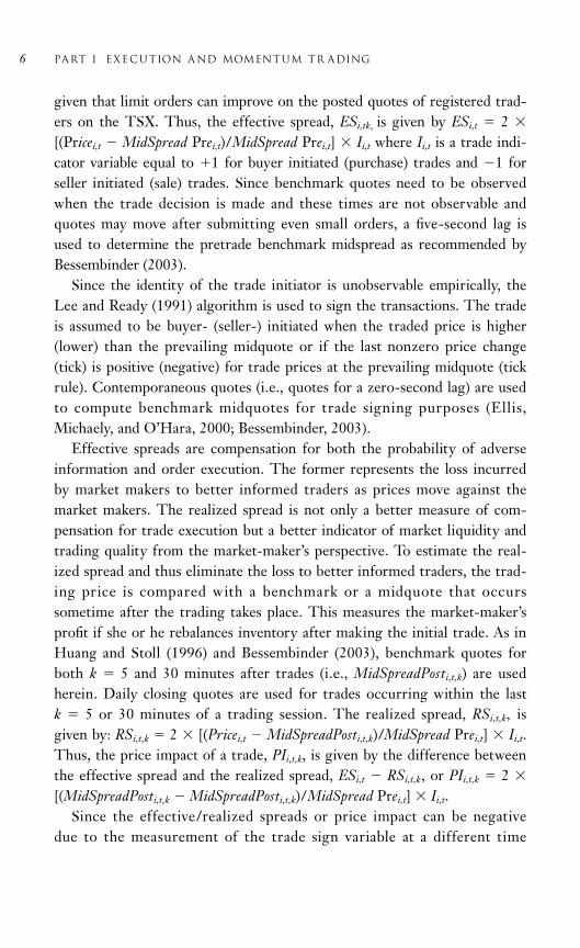
given that limit orders can improve on the posted quotes of registered trad-ers on the TSX. Thus, the effective spread, ESi,tk, is given by ESi,t 2
[(Pricei,t MidSpread Prei,t)/MidSpread Prei,t] Ii,t where Ii,t is a trade indi-cator variable equal to 1 for buyer initiated (purchase) trades and 1 forseller initiated (sale) trades. Since benchmark quotes need to be observedwhen the trade decision is made and these times are not observable andquotes may move after submitting even small orders, a five-second lag isused to determine the pretrade benchmark midspread as recommended byBessembinder (2003).
Since the identity of the trade initiator is unobservable empirically, theLee and Ready (1991) algorithm is used to sign the transactions. The tradeis assumed to be buyer- (seller-) initiated when the traded price is higher(lower) than the prevailing midquote or if the last nonzero price change(tick) is positive (negative) for trade prices at the prevailing midquote (tickrule). Contemporaneous quotes (i.e., quotes for a zero-second lag) are usedto compute benchmark midquotes for trade signing purposes (Ellis,Michaely, and O’Hara, 2000; Bessembinder, 2003).
Effective spreads are compensation for both the probability of adverseinformation and order execution. The former represents the loss incurredby market makers to better informed traders as prices move against themarket makers. The realized spread is not only a better measure of com-pensation for trade execution but a better indicator of market liquidity andtrading quality from the market-maker’s perspective. To estimate the real-ized spread and thus eliminate the loss to better informed traders, the trad-ing price is compared with a benchmark or a midquote that occurssometime after the trading takes place. This measures the market-maker’sprofit if she or he rebalances inventory after making the initial trade. As inHuang and Stoll (1996) and Bessembinder (2003), benchmark quotes forboth k 5 and 30 minutes after trades (i.e., MidSpreadPosti,t,k) are usedherein. Daily closing quotes are used for trades occurring within the last k 5 or 30 minutes of a trading session. The realized spread, RSi,t,k, isgiven by: RSi,t,k 2 [(Pricei,t MidSpreadPosti,t,k)/MidSpread Prei,t] Ii,t.Thus, the price impact of a trade, PIi,t,k, is given by the difference betweenthe effective spread and the realized spread, ESi,t RSi,t,k, or PIi,t,k 2 [(MidSpreadPosti,t,k MidSpreadPosti,t,k)/MidSpread Prei,t] Ii,t.
Since the effective/realized spreads or price impact can be negativedue to the measurement of the trade sign variable at a different time
6 Part i EXECUTION A ND MOMENTUM TR ADING

compared with the prevailing or subsequent quote, we also use an alter-native for these spread measures that relies on their absolute values. Forinstance, the alternative measure of the effective spread, AESi,t, is: AESi,t
2 |(Pricei,t MidSpread Prei,t)/MidSpread Prei,t|.The quoted dollar depth, which is the capacity of a market to absorb
trades with little or no price impact, also is measured to assess liquidityand market execution quality. As quotes represent prices at which marketmakers are willing to trade at a prespecified maximum trading size, weassume that this size is the highest possible volume before an order eatsup the available liquidity at the inside quotes and quotes need to be movedup or down depending on trade direction. We measure depth QDi,t, as theaverage quoted order flow size at both the inside bid and ask or QDi,t,
0.5 (Bidi,t BidSizei,t Aski,t AskSizei,t).
EMPIRICAL ESTIMATES FOR THE TSX
The relative quoted and effective spreads for all the securities listed onthe TSX and seven subsamples differentiated by security type (and pricein the case of common shares) are reported in Table 1.1. As expected, thelowest median spreads are for common shares with prices above $5 (Com-mon $5), followed by the asset-linked notes (NT_NO) for relativequoted spreads (QS) and preferred shares for the two measures of relativeand average effective spreads (ES and AES). The highest median spreadsare for Warrants. To illustrate, the median effective spreads are 0.31 per-cent and 6.88 percent for Common with prices above $5 and Warrants,respectively.
NT_NO and Common $5 are among the two lowest mean spreadswith Common $5 only occupying the lowest mean spread for the ESmeasure. Warrants have the highest mean spreads for each of the threemeasures. The relatively high trading costs associated with Warrants isprimarily due to the relatively low traded prices of Warrants (mean of$1.79 compared with $13.24 for all other securities). Securities denomi-nated in USD have the second highest mean and median spreads for all three measures. To illustrate, the median USD effective spread is 4.19 percent.
As expected, considerable variation exists in the spread measures withineach security type. The NT_NO followed by Common $5 have the lowest
chapter 1 Performance Leakage and Value Discounts 7
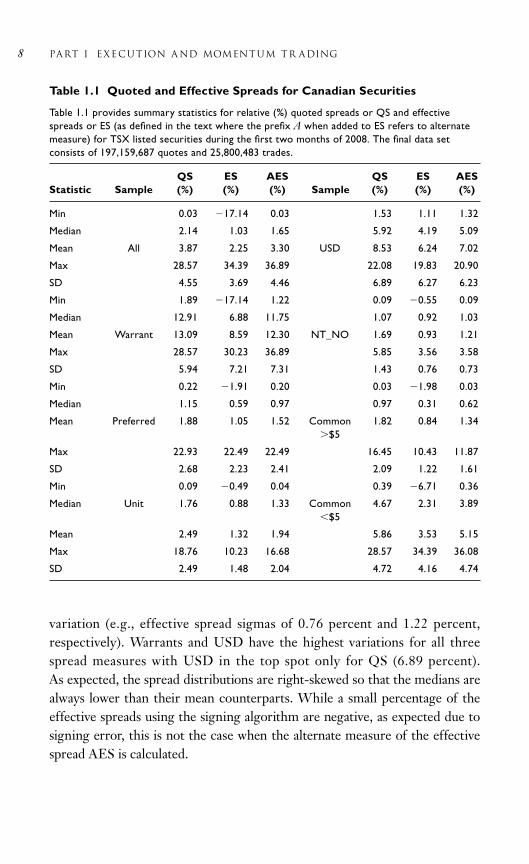
variation (e.g., effective spread sigmas of 0.76 percent and 1.22 percent,respectively). Warrants and USD have the highest variations for all threespread measures with USD in the top spot only for QS (6.89 percent). As expected, the spread distributions are right-skewed so that the medians arealways lower than their mean counterparts. While a small percentage of theeffective spreads using the signing algorithm are negative, as expected due tosigning error, this is not the case when the alternate measure of the effectivespread AES is calculated.
8 Part i EXECUTION A ND MOMENTUM TR ADING
Table 1.1 Quoted and Effective Spreads for Canadian Securities
Table 1.1 provides summary statistics for relative (%) quoted spreads or QS and effectivespreads or ES (as defined in the text where the prefix A when added to ES refers to alternatemeasure) for TSX listed securities during the first two months of 2008. The final data setconsists of 197,159,687 quotes and 25,800,483 trades.
QS ES AES QS ES AESStatistic Sample (%) (%) (%) Sample (%) (%) (%)
Min 0.03 17.14 0.03 1.53 1.11 1.32
Median 2.14 1.03 1.65 5.92 4.19 5.09
Mean All 3.87 2.25 3.30 USD 8.53 6.24 7.02
Max 28.57 34.39 36.89 22.08 19.83 20.90
SD 4.55 3.69 4.46 6.89 6.27 6.23
Min 1.89 17.14 1.22 0.09 0.55 0.09
Median 12.91 6.88 11.75 1.07 0.92 1.03
Mean Warrant 13.09 8.59 12.30 NT_NO 1.69 0.93 1.21
Max 28.57 30.23 36.89 5.85 3.56 3.58
SD 5.94 7.21 7.31 1.43 0.76 0.73
Min 0.22 1.91 0.20 0.03 1.98 0.03
Median 1.15 0.59 0.97 0.97 0.31 0.62
Mean Preferred 1.88 1.05 1.52 Common 1.82 0.84 1.34$5
Max 22.93 22.49 22.49 16.45 10.43 11.87
SD 2.68 2.23 2.41 2.09 1.22 1.61
Min 0.09 0.49 0.04 0.39 6.71 0.36
Median Unit 1.76 0.88 1.33 Common 4.67 2.31 3.89$5
Mean 2.49 1.32 1.94 5.86 3.53 5.15
Max 18.76 10.23 16.68 28.57 34.39 36.08
SD 2.49 1.48 2.04 4.72 4.16 4.74

A comparison of the mean, median, and sigma values for common sharestrading below and above $5 exemplifies the much higher trade costs associatedwith so-called “penny” stocks (e.g., median ES of 2.31 percent versus 0.31 percent and sigma of 4.16 percent versus 1.22 percent, respectively). Thismay have implications for small cap investing in national markets smaller thanin the United States.
The relative realized spreads for the various samples are reported inTable 1.2. With four exceptions (RS5 and RS30 for both USD and
chapter 1 Performance Leakage and Value Discounts 9
Table 1.2 Realized Spreads
Table 1.2 provides summary statistics for (%) realized spreads or RS (as defined in the textwhere the prefax A refers to alternate measure and the suffix 5 and 30 refer to quotes 5 and30 minutes, respectively, after trades) for TSX listed securities during the first two months of 2008.
RS5 ARS5 RS30 ARS30 RS5 ARS5 RS30 ARS30Statistic Sample (%) (%) (%) (%) Sample (%) (%) (%) (%)
Min 28.57 0.00 48.89 0.00 8.63 1.29 10.23 1.39
Median 1.20 1.84 1.16 2.11 1.23 6.06 2.79 4.92
Mean All 2.28 3.70 2.18 3.97 USD 0.60 8.18 1.64 6.05
Max 39.33 65.37 45.06 117.81 8.22 20.34 5.10 15.73
SD 3.65 5.49 3.88 6.04 5.24 6.69 4.31 4.16
Min 28.57 1.81 33.58 2.26 1.05 0.00 1.03 0.00
Median Warrant 6.03 12.28 5.52 13.00 NT_NO 0.83 1.25 0.96 1.21
Mean 7.13 14.91 6.97 16.01 0.75 1.74 0.86 1.66
Max 34.09 54.58 45.05 117.81 2.59 5.57 2.58 5.60
SD 8.42 10.66 9.41 14.69 0.82 1.45 0.75 1.34
Min 2.00 0.19 2.00 0.20 2.72 0.03 3.97 0.03
Median 0.72 1.03 0.71 1.05 0.43 0.90 0.41 1.37
Mean Preferred 1.19 1.56 1.17 1.61 Common 1.00 1.59 0.94 1.90$5
Max 21.43 21.43 21.43 21.43 10.58 10.98 10.58 11.44
SD 1.98 2.28 1.98 2.35 1.37 1.64 1.30 1.55
Min 0.03 0.04 0.60 0.05 19.05 0.37 48.89 0.36
Median 1.08 1.43 1.02 1.53 2.78 4.02 2.67 4.37
Mean Units 1.59 2.16 1.51 2.28 Common 3.62 5.55 3.41 5.86$5
Max 9.68 18.85 10.75 18.86 39.33 65.37 43.71 70.05
SD 1.66 2.34 1.61 2.29 4.07 5.87 4.48 5.84

NT_NO), the means are greater than their median counterparts, whichindicates right-skewed distributions. The median relative realized spreadsare lowest for Common $5 followed by Preferreds for all but theARS30 (Alteranative Realized Spread based on quotes 30 minutes aftertrades) measure where the lowest median is for Preferreds followed byNT_NO. To illustrate, the median RS5 and RS30 values are 0.43 per-cent and 0.41 percent, respectively, for Common $5. The highestmedian relative realized spreads are for Warrants. This is followed byCommon $5 for RS5 and by USD for the other three relative realizedspread measures.
The lowest mean RS5 and RS30 are for USD and NT_NO, respectively,followed by respectively NT_NO and Common $5. In contrast, the low-est mean ARS5 and ARS30 are for Preferreds followed by Common $5and NT_NO, respectively. Warrants always have the highest mean relativerealized spreads followed by Common $5 for RS5 and RS30 and by USDfor ARS5 and ARS30, respectively. Thus, the choice of how to calculate therelative realized spread has an impact on the rankings of this measureacross security types.
The lowest sigmas are found for NT_NO for all four relative realizedspread measures, followed by units for RS5 and Common $5 for theother three measures. Once again, Warrants have the highest relative real-ized spreads followed by USD for the two 5-minute measures and Com-mon $5 for the two 30-minute measures. To illustrate, the sigmas forRS5 and RS30 for Warrants are 8.42 percent and 9.41 percent, respectively.
The quoted depth-traded volumes (share numbers and dollars) and thenumber of trades for the various samples are reported in Table 1.3. All thedistributions are right-skewed. The lowest mean, median, and sigma ofquoted depth (QD), share volume (Shares vol) and number of trades are forWarrants, NT_NO, and NT_NO, respectively. With two exceptions, thehighest mean, median, and sigma of these three measures are for Common$5. The exceptions are NT_NO for the median QD and Common $5for the median Shares vol.
The high depth for the index linked notes shows that dealers have mini-mal concerns about trading against informed traders as private informationis negligible about the entire index compared with individual securities. Thehigh median of penny stock trading volume measured in number of sharesis due to the larger round lot sizes of stocks trading below $1 and the needto trade more shares of a lower priced share to achieve a comparable dollar
10 Part i EXECUTION A ND MOMENTUM TR ADING

Table 1.3 Quoted Depth and Trading Activity
Table 1.3 provides summary statistics for quoted depth (QD ($)), share volume (Shares vol), and dollar traded volume ($ Vol) in thousands, and number oftrades (Nb_trades) for TSX-listed securities during the first two months of 2008.
Statistic Sample QD ($) Shares vol $ Vol Nb_trades Sample QD ($) Shares vol $ Vol Nb_trades
Min 0.023 0.100 0.390 1.000 3.115 0.465 2.890 1.500
Median 9.761 25.550 93.318 12.929 12.066 3.321 31.706 5.033
Mean All 23.442 195.475 3,356.594 297.921 USD 15.324 36.295 96.264 5.675
Max 1,415.986 11,170.279 259,932.309 18,540.071 36.073 363.262 597.645 15.929
SD 73.373 663.623 17,206.560 1,222.051 9.441 108.491 174.238 3.831
Min 0.062 0.667 0.495 1.000 8.727 0.830 7.924 1.000
Median Warrant 1.138 24.578 14.767 5.099 NT_NO 26.003 2.750 29.576 1.857
Mean 4.445 75.745 70.674 11.646 32.595 4.066 44.990 2.357
Max 31.628 2,127.875 784.184 142.750 162.306 20.800 241.305 9.000
SD 6.912 211.431 147.433 19.117 27.205 3.971 45.936 1.604
Min 0.045 0.100 0.425 1.000 1.393 0.180 1.239 1.000
Median 15.395 4.042 76.289 6.225 Common $5 14.472 49.815 523.919 61.664
Mean Preferred 18.977 6.924 135.580 9.343 50.722 358.856 9,990.020 809.795
Max 107.109 85.414 2,154.335 57.333 1,415.986 8,686.755 259,932.309 18,540.071
SD 12.090 9.514 204.020 8.798 118.336 893.362 30,241.782 2,111.872
Min 0.358 0.425 2.079 1.125 0.023 0.350 0.390 1.000
Median 11.070 14.754 123.071 15.190 3.595 59.620 51.275 14.110
Mean Unit 16.178 79.108 1,300.092 153.898 Common $5 6.384 216.275 327.037 79.110
Max 1,261.424 2,074.231 52,655.592 3,884.548 148.640 11,170.279 2,2652.803 1,965.429
SD 63.361 185.596 4,357.675 429.569 13.721 750.003 1,240.112 204.073
11
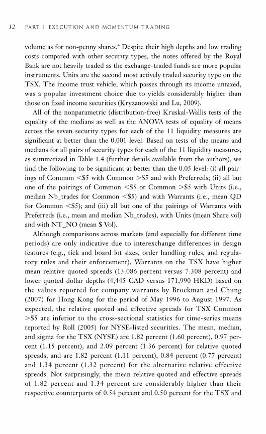
volume as for non-penny shares.4 Despite their high depths and low tradingcosts compared with other security types, the notes offered by the RoyalBank are not heavily traded as the exchange-traded funds are more popularinstruments. Units are the second most actively traded security type on theTSX. The income trust vehicle, which passes through its income untaxed,was a popular investment choice due to yields considerably higher thanthose on fixed income securities (Kryzanowski and Lu, 2009).
All of the nonparametric (distribution-free) Kruskal-Wallis tests of theequality of the medians as well as the ANOVA tests of equality of meansacross the seven security types for each of the 11 liquidity measures aresignificant at better than the 0.001 level. Based on tests of the means andmedians for all pairs of security types for each of the 11 liquidity measures,as summarized in Table 1.4 (further details available from the authors), wefind the following to be significant at better than the 0.05 level: (i) all pair-ings of Common $5 with Common $5 and with Preferreds; (ii) all butone of the pairings of Common $5 or Common $5 with Units (i.e.,median Nb_trades for Common $5) and with Warrants (i.e., mean QDfor Common $5); and (iii) all but one of the pairings of Warrants withPreferreds (i.e., mean and median Nb_trades), with Units (mean Share vol)and with NT_NO (mean $ Vol).
Although comparisons across markets (and especially for different timeperiods) are only indicative due to interexchange differences in designfeatures (e.g., tick and board lot sizes, order handling rules, and regula-tory rules and their enforcement), Warrants on the TSX have highermean relative quoted spreads (13.086 percent versus 7.308 percent) andlower quoted dollar depths (4,445 CAD versus 171,990 HKD) based onthe values reported for company warrants by Brockman and Chung(2007) for Hong Kong for the period of May 1996 to August 1997. Asexpected, the relative quoted and effective spreads for TSX Common$5 are inferior to the cross-sectional statistics for time-series meansreported by Roll (2005) for NYSE-listed securities. The mean, median,and sigma for the TSX (NYSE) are 1.82 percent (1.60 percent), 0.97 per-cent (1.15 percent), and 2.09 percent (1.36 percent) for relative quotedspreads, and are 1.82 percent (1.11 percent), 0.84 percent (0.77 percent)and 1.34 percent (1.32 percent) for the alternative relative effectivespreads. Not surprisingly, the mean relative quoted and effective spreadsof 1.82 percent and 1.34 percent are considerably higher than theirrespective counterparts of 0.54 percent and 0.50 percent for the TSX and
12 Part i EXECUTION A ND MOMENTUM TR ADING

13
Table 1.4 Tests of Pairwise Means and Medians for the Various Liquidity Measures
Table 1.4 reports the liquidity measures with p values 0.05 for tests of pairwise means and medians, which are reported in the lower and upper diagonals,respectively. Thus, they are not reported (such as between Common $5 and Common $5) if they are significant at the 0.05 level. They are underlined ifthe pairwise differences are significant at the 0.10 level.
Common CommonWarrant Preferred Unit USD NT_TO $5 $5
Warrant Nb_trades $ Vol, Nb_trades, ES
Preferred Nb_trades QD, Shares vol, QS, ES, AES, QDNb_trades, RS5 (A)RS5 & 30
Unit Shares vol QD, ES QD, RS5, RS30 QS, ES, AES, Nb_tradesARS5, (A)RS30
USD Shares & $ Vol, QD, $ Vol, QD, Shares & $ Vol, Shares & $ QS, $ Vol, AES, QD, RS5Nb_trades, Nb_trades, Nb_trades, Vol, RS5 (A)RS5 & 30ES, RS30 RS5 & 30 RS5, RS30
NT_NO $ Vol QS, Shares vol, QD, $ Vol, $ Vol, RS5&30 QS, (A)RS5 & 30(A)ES, (A)RS5, ES, ARS5,(A)RS30 ARS30
Common $5 QD QS, Shares & $ Vol, Shares & $ VolNb_trades, AES,ARS5, (A)RS30
Common $5 QS, ES, AES, QD, Shares & $ Vol, QS, QD, (A)ES,(A)RS5, RS30 Nb_trades, RS5 & 30 (A)RS5 & 30

considerably lower than their respective counterparts of 2.32 percent and 2.13 percent for the average exchange, which are reported by Jain(2003) based on closing daily values for the 25 highest market capitaliza-tion stocks for each of 51 major exchanges for the first four months of 2000.
Time-series plots of six of the liquidity measures for the various samplesare depicted in Figures 1.1 to 1.6. We examine the intertemporal variationin these series using the standard deviation (sigma) and coefficient of varia-tion (i.e., the sigma divided by the mean).
Based on untabulated results, the three security types with the highestspread sigmas are Warrants followed by USD and NT_NO for QS and aninterchange of Warrants and NT_NO for ES and RS30. The three securitytypes with the highest spread Coefficients of Variation (CVs) are NT_NOfollowed by USD and Preferreds for QS, and USD followed by NT_NO
14 Part i EXECUTION A ND MOMENTUM TR ADING
Warrant
Warrant
14
12
10
8
6
4
2
0
0102
0104
0108
0110
0114
0116
0118
0122
0124
0128
0130
0201
0205
0207
0211
0213
0215
0220
0222
0226
0228
Date—Daily first 2 months 2008
NT_NO
USD
Med
ian
Rel
ativ
e Q
uote
d S
prea
d (%
)
USD
Com<$5
AllCom>$5UnitPreferred
Figure 1.1 Time-Series of Median Relative Quoted Spreads (%)

chapter 1 Performance Leakage and Value Discounts 15
USD
35
30
25
20
15
10
5
0
Date—Daily first 2 months 2008
Med
ian
Quo
ted
Dep
th (
$000
)
NT_NO
USDCom<$5Warrant
Preferred
UnitCom>$5All
0102
0104
0108
0110
0114
0116
0118
0122
0124
0128
0130
0201
0205
0207
0211
0213
0215
0220
0222
0226
0228
Figure 1.2 Time-Series of Median Quoted Depths (in thousands of $)
8.00
7.00
6.00
5.00
4.00
3.00
2.00
1.00
0.00
Date—Daily first 2 months 2008
Med
ian
Rel
ativ
e E
ffec
tive
Spr
ead
(%)
NT_NOAllCom>$5Unit
Warrant
Warrant
Preferred
USD
USD
Com>$5
0102
0104
0108
0110
0114
0116
0118
0122
0124
0128
0130
0201
0205
0207
0211
0213
0215
0220
0222
0226
0228
Figure 1.3 Time-Series of Relative Effective Spreads (%)

16 Part i EXECUTION A ND MOMENTUM TR ADING
12
10
8
6
4
2
0
2
Date—Daily first 2 months 2008
Med
ian
Rel
ativ
e R
ealiz
ed S
prea
d (%
)
NT_NOAll; Com>$5;Unit; Preferred
Warrant
USD
USD
USD
Com>$5
0102
0104
0108
0110
0114
0116
0118
0122
0124
0128
0130
0201
0205
0207
0211
0213
0215
0220
0222
0226
0228
Figure 1.4 Time-Series of Relative 30-Minute Post-Realized Spreads (%)
180
160
140
120
100
80
60
40
20
0
Date—Daily first 2 months 2008
Med
ian
Vo
lum
e ($
000)
NT_NO
Com>$5Unit
Unit
WarrantUSD
Com<$5
0102
0104
0108
0110
0114
0116
0118
0122
0124
0128
0130
0201
0205
0207
0211
0213
0215
0220
0222
0226
0228
Preferred
All
Figure 1.5 Time-Series of Dollar Volume (in thousands of $)

and Warrants for ES and RS30. The security types with the largest QD ($)sigmas are NT_NO followed by USD and Preferreds, and with the largestQD ($), CVs are USD followed by Warrants and NT_NO. The securitytypes with the largest $ Vol sigmas are NT_NO followed by Units andUSD, and with the largest $ Vol CVs are NT_NO followed by USD andWarrants. The security types with the largest Nb_trade sigmas are Unitsfollowed by USD and Common $5, and with the largest Nb_trade CVsare USD followed by NT_NO and Preferreds.
Thus, Common $5 never appear and Common $5 only appears oncein the top three ranks for intertemporal variation for all six depicted liquidity measures. Units appear in the top three ranks for intertermporalvariation for only the two trade-activity measures of liquidity. WhileNT_NO has relatively low spreads and high quoted depths compared withthe other security types, it has relatively lower trade-activity measures ofliquidity and relatively higher intertemporal variation for all six liquiditymeasures.
chapter 1 Performance Leakage and Value Discounts 17
25
20
15
5
0
10
Date—Daily first 2 months 2008
Num
ber
of T
rade
s
NT_NO
Com>$5;Com<$5
Unit
Warrant
USD
0102
0104
0108
0110
0114
0116
0118
0122
0124
0128
0130
0201
0205
0207
0211
0213
0215
0220
0222
0226
0228
Preferred
Preferred
All
Figure 1.6 Time-Series of Number of Trades

The behavior of the six liquidity measures in Figures 1.1 to 1.6 aroundMonday, January 21, 2008 is interesting. Just prior to and on this date,world equity markets were affected adversely due to worries of a globalrecession. There was an upward spike in relative spreads (quoted andeffective and especially for Warrants), and an upward spike in dollartraded volume.
CONCLUSION
This chapter makes four major contributions to the literature and prac-tice. First, this study provides estimates of various measures of trade execution quality that investors must seriously consider when deciding toeffect investment decisions, and documents signif icant dif ferences in potential and actual trade execution costs as measured by various mar-ket qualit y measures intra- and inter-security t ype and across time(intertemporally). This information should be of considerable interest toinvestors (especially technical traders) who must carefully balance themarginal benefits and costs of each transaction. Second, this study pro-vides estimates of the magnitudes of the discounts required when valuingvarious security types under a hold scenario and under less and morepatient liquidation scenarios. This information should be of considerableinterest to asset valuators and to investors when assessing the value ofmutual funds with concentrated or nongranular portfolios under variousexit strategies for specific security holdings. Third, this study providesestimates of the discounts required when assessing reported portfolioperformance. This performance-drag information should be of consider-able interest to investors in all funds that actively trade, and particularlyin those funds with aggressive and nongranular holdings and limited liq-uidity provisions under down-market scenarios. Fourth, this study docu-ments how trade execution costs vary on a daily basis and how they areaffected adversely by worries of a global recession (i.e., prior to and onMonday, January 21, 2008).
ACKNOWLEDGMENTS
Financial support from the Autorité des Marchés Financiers, ConcordiaUniversity Research Chair in Finance, IFM2, and SSHRC are gratefully
18 Part i EXECUTION A ND MOMENTUM TR ADING

acknowledged. The usual disclaimer applies in that the views expressedherein are solely the authors’ own and do not necessarily reflect the offi-cial positions or policies of the providers of financial support of thischapter or the views of their staff members or the institutions that theywork for.
REFERENCES
Bessembinder, H. (2003) Issues in Assessing Trade Execution Costs. Journal of Financial Markets, 6(3): 233–257.
Bodurtha, S.G. and Quinn, T.E. (1990) Does Patient Program TradingReally Pay? Financial Analysts Journal, 46(3): 35–42.
Boehmer, E. (2005) Dimensions of Execution Quality: Recent Evidencefor U.S. Equit y Markets. Journal of Financial Economics, 78(3):463–704.
Brockman, P. and Chung, D.Y. (2007) Chapter 2: Liquidity Provision in theHong Kong Warrant Market: Evidence from Equity, Derivative andBasket Warrants. In: Lhabitant, F.-S. and Gregoriou, G.N. (eds.), StockMarket Liquidity: Implications for Market Microstructure and AssetPricing. John Wiley & Sons: New York.
Chordia, T., Roll R., and Subrahmanyam, A. (2001) Market Liquidity andTrading Activity. Journal of Finance, 56(2): 501–530.
Collins, B.M. and Fabozzi, F.J. (1991) A Methodology for MeasuringTransaction Costs. Financial Analysts Journal, 47(2): 27–36, 44.
Eleswarapu, V. and Venkataraman, K. (2006) The Impact of Legal and Polit-ical Institutions on Equity Trading Costs: A Cross-country Analysis.Review of Financial Studies, 19(3): 1081–1111.
Ellis, K., Michaely R., and O’Hara, M. (2000) The Accuracy of TradeClassification Rules: Evidence from Nasdaq. Journal of Financial andQuantitative Analysis, 35(4): 529–551.
Hasbrouck, J. (2009) Trading Costs and Returns for U.S. Equities: EstimatingEffective Costs from Daily Data. Journal of Finance, 64(3): 1445–1477.
Huang, R. and Stoll, H. (1996) Dealer versus Auction Markets: A PairedComparison of Execution Costs on NASDAQ and NYSE. Journal ofFinancial Economics 41(3): 313–357.
chapter 1 Performance Leakage and Value Discounts 19
Jain, P.K. (2003) Institutional Design and Liquidity at Stock Exchangesaround the World. Working paper, University of Memphis, Memphis,TN. Available at: http://ssrn.com/abstract869253
Kothare, M. and Laux, P.A. (1995) Trading Costs and the Trading Systemsfor Nasdaq Stocks. Financial Analysts Journal, 51(2): 42–53.
Kryzanowski, L. and Lu, Y. (2009) In Government We Trust: Rise and Fallof Canadian Business Income Trust Conversions. Managerial Finance,35(9): 784–802.
Lee, C. and Ready, M.J. (1991) Inferring Trade Directions from IntradayData. Journal of Finance, 46(2): 733–746.
Roll, R. (2005) Recent Research on Liquidity. Keynote address, NorthernFinance Association, Vancouver, BC. Available at: http://www.chaire-produits-derives.uqam.ca/pages/transfert.asp?dtransfert&pseminaires
SEC. (2001) Report on the Comparison of Order Executions Across EquityMarket Structures. Office of Economic Analysis, United States Securi-ties and Exchange Commission: Washington, DC; January 8. Availableat: http://www.sec.gov/pdf/ordrxmkt.pdf
Venkataraman, K. (2001) Automated Versus Floor Trading: An Analysis ofExecution Costs on the Paris and New York Exchanges. Journal ofFinance, 56(4): 1445–1485.
Wagner, W.H. and Edwards, M. (1993) Best Execution. Financial AnalystsJournal, 49(1): 65–71.
Wilcox, J.W. (1993) The Effect of Transaction Costs and Delay on Perfor-mance Drag. Financial Analysts Journal, 49(2): 45–54, 77.
NOTES
1. This security type is not examined subsequently because no tradingactivity for debentures (ticker suffix DB) is found in the TAQ database.
2. Using the TSX eReview, only one security is identified as having aticker symbol change. On January 21, 2008, the ticker of NordResources Corporation changed from NRD.U to NRD. Similarly,only two securities (Absolute Software Corporation and CorusEntertainment Inc B class) had subdivisions during the studiedperiod.
20 Part i EXECUTION A ND MOMENTUM TR ADING

3. Quotes with extremely high spreads are usually passive in the sense thateither the bid or the offer (or both) are posted away from competitiveprices.
4. On the TSX, board lot sizes are 100, 500, and 1,000 units for tradingprices per unit of $1 or more, $0.10 to $0.99, and less than $0.10,respectively.
chapter 1 Performance Leakage and Value Discounts 21

This page intentionally left blank

23
2C H A P T E R
Informed Tradingin Parallel Auctionand Dealer Markets The Case of the London Stock Exchange
Pankaj K. Jain, Christine Jiang, Thomas H. McInish,and Nareerat Taechapiroontong
ABSTRACT
In this chapter, we examine trading on the London Stock Exchange wherethe same stocks trade side-by-side on the computer-based Stock ExchangeElectronic Trading Service (SETS) and the dealer market (DM). SETS hasmore trades overall, but the DM has larger trades and dominates the execu-tion of very large-sized trades. The permanent price impact of trades ismuch larger on SETS than on the DM. However, the temporary priceimpact of trades is significantly larger on the DM than on SETS. The twoeffects together indicate that informed trades are likely routed to SETS forimmediate execution, whereas informed trades are screened or trade pricesare appropriately negotiated ex-ante to reflect information in the DM.
INTRODUCTION
We study trading on the London Stock Exchange (LSE) where, unlikemost other exchanges, the same stocks trade on the computer-based StockExchange Electronic Trading Service (SETS) and the dealer market (DM).

SETS is the fully computerized automated trading system where liquidityis provided by traders who submit limit orders. The purpose of our chapteris to analyze informed order flows and price impact of trades in this parallelmarket structure.
At the time of our study, dealers had no affirmative obligation to offerquotes. Yet, the DM accounts for a significant share of trading volume.Dealers can also provide liquidity on SETS. There is no requirement forformal interaction between SETS and the DM. Yet SETS and DM are veryclosely integrated and may often have the same dealer serving as counter-party. Nevertheless, there are several important distinctions between thetwo systems in terms of anonymity and direct agency crosses. The hybridstructure of the LSE has not yet been examined in the context of informedtrading, although other studies analyze the interaction of order f lowbetween the two markets (see Friederich and Payne, 2007) and the dynam-ics of the market open and close (see Ellul, Shin, and Tonks, 2005).
We provide a number of findings. Both the SETS and the DM are activewith the SETS market executing more trades, but the DM executing largertrades overall and dominating the execution of very large trades. The per-manent price impact of trades is not only significantly lower on the DMthan on SETS, but is actually negative. However, the temporary priceimpact of trades is significantly larger on the DM than on SETS. The tworesults together suggest that dealers on the DM are able to effectively iden-tify informed trades ex-ante. Such identification of trade motives enablesdealers to either screen out the informed trades avoiding losses or tradeeffectively with them, and in the process learning the information withwhich they can trade profitably for their own accounts, as suggested byNaik, Neuberger, and Viswanathan (1999).
TRADING SYSTEMS AND VENUES
Competing yet Complementary Trading Systems
Madhavan (1995) proposes a model that provides a rationale for the exis-tence of fragmented markets, focusing on the impact of disclosing tradinginformation to market participants. He shows that informed traders andlarge traders who place multiple trades obtain lower expected trading costsin fragmented markets where their trades are not disclosed. On the otherhand, dealers benefit from nondisclosure by decreasing price competition.
24 Part i EXECUTION A ND MOMENTUM TR ADING

Contrary to this view, Chowdhry and Nanda (1991) provide a theoreticalmodel in which if more than one market for a security exists, one marketwill emerge as the dominant market, a “winner takes most” phenomenon.This prediction occurs as liquidity traders seek thick markets with the low-est execution costs and informed traders maximize their profits by hidingtrades in the most liquid markets. Glosten (1994) suggests that the openelectronic limit order book such as SETS is inevitable because it provides asmuch liquidity as possible in extreme situations and does not invite compe-tition from third market dealers, while other trading institutions do.
Our empirical analysis presented later is consistent with the coexistencehypothesis instead of the market dominance hypothesis.
Permanent Price Impact in Coexisting Markets
Another branch of literature allows for coexistence and deals with eitherupstairs versus downstairs markets or auction versus dealer markets. Seppi(1990), Easley and O’Hara (1987), and Easley, Kiefer, and O’Hara (1996)developed models in which dealers (such as upstairs block traders in New York or the dealers in London) are able to differentiate uninformedtraders from informed traders based on reputation signals or other implicitcommitments. This non-anonymous feature in dealer markets enables ex-ante identification, relationship based information sharing as suggestedby Hansch, Naik, and Viswanathan (1999), or potential cream skimming ofuninformed trades and screening out of informed traders. This ability ofthe dealers lowers adverse selection costs for large liquidity traders. Seppi(1990) argues that the lack of anonymity in off-exchange block tradingenables investors and the dealers to make “no bagging the street” commit-ments and face penalties on any subsequent trades if they fail to divulgeinformation.
Grossman (1992), Pagano and Roell (1996), and Schwartz and Steil(1996) focus on order transparency in limit order books like SETS. Theysuggest that many large traders do not want to expose their orders to thepublic since large trades may adversely impact the market price, may invitefront running by other traders, and may introduce a free-option problem(the risk of being picked off if market conditions change). A large order sentto the DM is less exposed than one sent to the SETS market and may bematched with other unexpressed liquidity. As a consequence, dealers serveas a repository of information on large investors’ latent trading interest.
chapter 2 Informed Trading in Parallel markets 25

Premiums paid to the dealers by informed traders are justified if they areless than costs of marching up or down the order book to execute largequantities. We examine these predictions of the theoretical models in outunivariate analysis of the unique hybrid LSE market structure. Additionally,Franke and Hess (2000) propose that the information differential betweenan anonymous screen-based trading system and a non-anonymous floortrading system should increase the attractiveness of the latter in the times ofhigh information intensity (proxies for information intensity include tradingvolume and price volatility). We study these ideas in our cross-sectionalregression.
A few country specific empirical studies are closely related to ours. Heidle and Huang (2002) investigate whether auction markets (NYSE,AMEX) or dealer markets (NASDAQ) are better able to identify informedtraders. Gramming, Schiereck, and Theissen (2001) examine the relation ofdegree of trader anonymity and the probability of informed trading on thetwo parallel markets at the Frankfurt Stock Exchange. Booth et al. (2002)and Smith, Turnbull, and White (2001) find that upstairs trades have alower permanent price impact than those executed downstairs in Helsinkiand Toronto, respectively. Our chapter extends the analysis to the hybridLSE market and also analyzes both permanent and temporary priceimpacts. The former unveils the informativeness of trades, whereas the latter represents the transaction cost for investors.
Temporary Price Impact in Auction and Dealer Markets
As addressed in Seppi (1990) and Grossman (1992), off-exchange dealermarkets involve a process of searching and matching of order flow. Tempo-rary price concessions are needed to induce dealers to accommodate ordersdue to inventory holding risk. On the other hand, SETS is fully automatedimplying that additional liquidity cannot be negotiated by the offer ofprice concessions. Hence, trade sizes and temporary price impacts shouldbe larger for an off-exchange DM than for an anonymous SETS market.In addition, for small sizes, dealers may not offer significant price improve-ment because of less intensive competition. For large orders, dealers havethe ability to extract additional information about the motivation behindthe order flow and benefit from such reputation effects, and significantprice improvements are often achieved as a result. Thus, temporary price
26 Part i EXECUTION A ND MOMENTUM TR ADING

impact is a decreasing function of trade size for orders on the DM market.Bernhardt et al. (2005) also develop a model along these lines where largerorders have lower transaction costs on the LSE.
INSTITUTIONAL BACKGROUND, DATA, AND METHODOLOGY
The London Stock Exchange
The London Stock Exchange, which is one of world’s leading stock exchanges,has experienced significant transformation to maintain and compete for orderflow and to improve price discovery. Before October 1997, the LSE was apure quote-driven dealer market (Stock Exchange Automated Quotation,SEAQ) with relatively nontransparent order flow. Retail investors complainedthat they were subsidizing large traders, which caused order flow to migrate toother European markets.
In 1997, the LSE began to implement a phased introduction of a moretransparent order-driven auction market called the Stock Exchange Elec-tronic Trading System. At first, SETS traded stocks in the FTSE 100index, but over time the stocks covered increased and in 2003 roughly 217stocks from the FTSE 250 index were traded. Thin stocks that have neverbeen components of these two indices are traded only on an old quote-driven market (SEAQ) and are not included in our study.1
Dealers on the LSE can compete voluntarily for trades on SETS’ stockson an off-exchange DM, but are no longer obliged to post firm bid and askprices as they did earlier, and their quotes are no longer available to investorsthrough a publicly available price-display mechanism. Trades on the DM arenot constrained by limit order prices on SETS or required to be partiallyexecuted against the limit order book. This arrangement differs from otherhybrid markets such as the NYSE, Toronto Stock Exchange, Paris Bourse,or Helsinki Stock Exchange where the public orders in the limit order takepriority over specialist market maker’s own trades. Investors can choosetheir trading venues depending on their motivation. Investors, who requireprompt and anonymous transactions, may prefer to execute market ordersagainst the book in SETS. Passive customers may choose to place limitorders on the book. Large traders, who do not want their trades to createextensive impact on prices in an order book market, may prefer to trade off-book on the DM. For additional institutional details about the LSE, seeBoard and Wells (2001) and Friederich and Payne (2007).
chapter 2 Informed Trading in Parallel markets 27

Data Selection and Processing
This study uses data provided by the London Stock Exchange for stocksthat are components of either the FTSE 100 or FTSE 250 indices in 2000,designated as SET1 or SET2. These stocks are traded on both the SETSand the DM. We include only trades during normal hours (08:00 to 16:30).All trades are in GBP.
These data comprise a number of files. For each trade, the TradeReports File has the firm symbol, date, time, price, number of shares,whether the trade is buyer or seller initiated, which market was used for thetrade (SETS or DM), type of order (market, limit), special designations(such as fill or kill), and the settlement date. We note that in determiningtrade direction on the DM we take the viewpoint of a trader. We excludetrades with settlement dates greater than SETS’ standard settlement date, trades with a price or volume of zero, and trades with size greaterthan 8 NMS and trades designated “WT” (which are 8 NMS and are sub-ject to a Work Principal Agreement), “UT” (occurring during opening andclosing call period), “RO” (resulting from an option exercise), “SW”(resulting from a stock swap), “CT” (contra trades), and “PN” (work prin-cipal portfolio notification). We also exclude trades for which the quantity|( pt pt1) /pt1|0.5 where pt is the trade price at time t, as this conditionmight result from potential data entry errors.
All quote data are from SETS. The DM does not provide quote data.The Best Prices File includes the time and price (but not the depth) of allquote updates that are better than an existing bid or ask on SETS. Weexclude quotes with either ask, bid, ask size, or bid size less than or equal tozero, and for which |(atat1)/at1|0.5 or |(btbt1)/bt1|0.5, where at
is the ask quote and bt is the bid quote.For all orders submitted to SETS, the Order History File contains
details about the date and time when the order is entered, deleted, can-celled, or executed, along with its order type, quantity, and limit price. Weuse these details to obtain aggregate depth at each best limit price.
Due to mergers, new listings, and delistings, stocks leave and join theindex during the year and to ensure a sufficient sample period, we use onlystocks that are members of either index for at least 80 days during the year2000. The final sample comprises 177 firms after deleting 16 stocks notmeeting the requirements enumerated above. The average market capital-ization for these firms, obtained from the Compustat global file, is 7.5 bil-lion pounds and the average stock price is 6.59 pounds.
28 Part i EXECUTION A ND MOMENTUM TR ADING

Measurement of Price Impact
To measure whether there is a difference in how trades affect prices onSETS and the DM, we use the method of Keim and Madhavan (1996) andBooth et al. (2002). This method uses trade prices rather than quotes,which is helpful because we do not have quotes for the DM. The total priceimpact can be decomposed into the permanent price impact and the tempo-rary price impact. The permanent price impact reflects changes in beliefsabout a security’s value due to new information conveyed by trades.2 Thetemporary price impact measures liquidity effects from transitory pricereversals. The total price impact reflects the difference between the tradeprice required to absorb the order and the preceding price.
We assume that a trade occurs at time t with price PT. The equilibriumprice observed at time t b before trade at time t is PB and the equilibriumprice observed at time t a after trade at time t is PA. The sequence oftrades is b t a. We measure price impact as
Permanent price impact (%) BS ln (PA/PB) 100 (2.1)
Temporary price impact (%) BS ln (PT/PA) 100 (2.2)
Total price impact (%) BS ln (PT/PB) 100 (2.3)
where BS equals plus (minus) 1 for buyer (seller) initiated trades. We alsostudy differences in price impact by trade size. We categorize trades by per-centiles of all trades for each firm. This ensures a representation of allstocks in each trade size category rather than bunching of trades from astock in one category. Note that the trade size cut-off varies from firm tofirm. To identify the equilibrium prices before and after a trade, we plot theprice movement around large GBP trades (top 5 percent in terms of GBP)in Figure 2.1. We calculate cumulative returns as follows. Each trade islabeled as trade 0, in turn. The previous 20 trades (regardless of trade loca-tion, size, buy/sell) executed prior to trade 0 (1, 2, . . .,20) and 20trades executed after trades 0 (1, 2, . . ., 20) are obtained. Then trade-to-trade returns calculated as the difference in log prices are estimatedfrom each trade from trade 20 to trade 20. These returns are averagedand cumulated.
We identify the 5 percent of trades that have the greatest GBP value. Welabel each of these trades, in turn, as trade 0. For each trade 0, we identifythe 20 previous trades, trades 1 through 21, and the subsequent 21
chapter 2 Informed Trading in Parallel markets 29
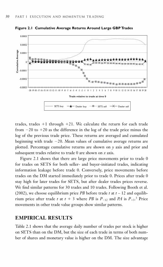
trades, trades 1 through 21. We calculate the return for each tradefrom 20 to 20 as the difference in the log of the trade price minus thelog of the previous trade price. These returns are averaged and cumulatedbeginning with trade 20. Mean values of cumulative average returns areplotted. Percentage cumulative returns are shown on y axis and prior andsubsequent trades relative to trade 0 are shown on x axis.
Figure 2.1 shows that there are large price movements prior to trade 0for trades on SETS for both seller- and buyer-initiated trades, indicatinginformation leakage before trade 0. Conversely, price movements beforetrades on the DM started immediately prior to trade 0. Prices after trade 0stay high for later trades for SETS, but after dealer trades prices reverse.We find similar patterns for 30 trades and 10 trades. Following Booth et al.(2002), we choose equilibrium price PB before trade t at t – 12 and equilib-rium price after trade t at t 3 where PB is P12 and PA is P3.3 Pricemovements in other trade value groups show similar patterns.
EMPIRICAL RESULTS
Table 2.1 shows that the average daily number of trades per stock is higheron SETS than on the DM, but the size of each trade in terms of both num-ber of shares and monetary value is higher on the DM. The size advantage
30 Part i EXECUTION A ND MOMENTUM TR ADING
Trade relative to trade at time 0
Cum
ulat
ive
Ave
rage
0.0003
0.0001
-0.0001
-0.0002
-0.0003-20 -19 -18 -17 -16 -15 -14 -13 -12 -11 -10 -9 -8 -7 -6 -5 -4 -3 -2 -1 0 1 2 3 4 5 6 7 8 9 10 11 12 13 14 15 16 17 18 19 20
0
0.0002
Dealer buySETS buy SETS sell Dealer sell
Figure 2.1 Cumulative Average Returns Around Large GBP Trades

of the DM is evident even though these data exclude trades that are greaterthan 8 NMS, which are mostly DM trades. Both quoted and effectivespreads are higher on SETS at the time orders are submitted to the DMthan at other times. The higher effective spread on SETS at the time whenorders are sent to the DM shows that many traders are actually timing theirtrading venue and switching to the DM under particular conditions. Weview this as the purchase of (high-cost) liquidity when this liquidity is notavailable on SETS.
For 2000, we present summary statistics for our sample of 149 firms.The overall SETS and DM results are presented in columns 2 to 4. Thefirst three rows present the daily number of trades, number of shares tradedand GBP trading volume. Return volatility is the standard deviation ofhourly returns in percentage. Trade size is the average number of shares foreach trade and GBP trade size is the monetary value of each trade. SETS’relative quoted-spread (%) is computed as (ask bid)/(ask bid)/2100immediately prior to the trades. SETS Effective spread is the absolute valueof the difference between the trade price and the midpoint of the spread atthe time of the trade. Depth at best bid and ask immediately prior to the
chapter 2 Informed Trading in Parallel markets 31
Table 2.1 Summary Statistics
t test of Mean Difference between
All SETS DM SETS and DM
Number of trades per day per stock 294 163 131 32*
Thousands of shares traded per stock per day 3,201 1,496 1,706 210*
GBP trading volume in thousands 19,520 9,266 10,256 990*
Return volatility (%) 1.60 1.20 1.58 0.38*
Trade size 10,696 8,536 14,539 6,003*
GBP trade size 50,560 40,347 68,901 28,554*
SETS’ relative quoted-spread (%) 0.987 0.933 1.046 0.114*
Effective spread (%) 0.705 0.201 0.617 0.416*
SETS depth 48,693 55,669 40,298 15,371*
GBP SETS depth (000s) 239,295 273,024 189,550 83,475*
* Significant at the 0.01 level.
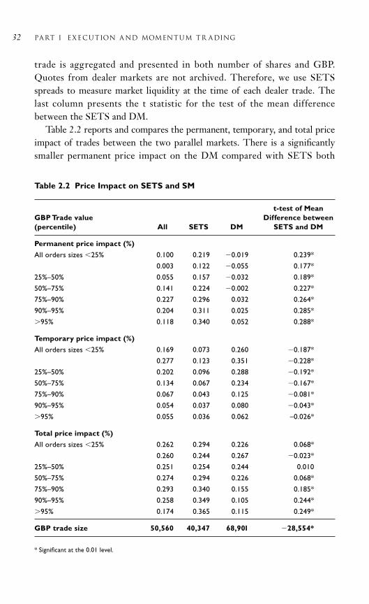
trade is aggregated and presented in both number of shares and GBP.Quotes from dealer markets are not archived. Therefore, we use SETSspreads to measure market liquidity at the time of each dealer trade. Thelast column presents the t statistic for the test of the mean differencebetween the SETS and DM.
Table 2.2 reports and compares the permanent, temporary, and total priceimpact of trades between the two parallel markets. There is a significantlysmaller permanent price impact on the DM compared with SETS both
32 Part i EXECUTION A ND MOMENTUM TR ADING
Table 2.2 Price Impact on SETS and SM
t-test of MeanGBP Trade value Difference between(percentile) All SETS DM SETS and DM
Permanent price impact (%)
All orders sizes 25% 0.100 0.219 0.019 0.239*
0.003 0.122 0.055 0.177*
25%–50% 0.055 0.157 0.032 0.189*
50%–75% 0.141 0.224 0.002 0.227*
75%–90% 0.227 0.296 0.032 0.264*
90%–95% 0.204 0.311 0.025 0.285*
95% 0.118 0.340 0.052 0.288*
Temporary price impact (%)
All orders sizes 25% 0.169 0.073 0.260 0.187*
0.277 0.123 0.351 0.228*
25%–50% 0.202 0.096 0.288 0.192*
50%–75% 0.134 0.067 0.234 0.167*
75%–90% 0.067 0.043 0.125 0.081*
90%–95% 0.054 0.037 0.080 0.043*
95% 0.055 0.036 0.062 –0.026*
Total price impact (%)
All orders sizes 25% 0.262 0.294 0.226 0.068*
0.260 0.244 0.267 0.023*
25%–50% 0.251 0.254 0.244 0.010
50%–75% 0.274 0.294 0.226 0.068*
75%–90% 0.293 0.340 0.155 0.185*
90%–95% 0.258 0.349 0.105 0.244*
95% 0.174 0.365 0.115 0.249*
GBP trade size 50,560 40,347 68,901 28,554*
* Significant at the 0.01 level.

overall and for each size category. This is quite contrary to the notion thattheoretical models and empirical works suggest, that is, informed tradersprefer to trade in anonymous dealer systems where they do not have to dis-close their trading interest ex-ante to the public. Barclay, Hendershott, andMcCormick (2003) report that there is a tendency for informed trades inNASDAQ to migrate to anonymous electronic communication networks.Our explanation for the lower permanent price impact lies in that the uniquefeatures of the DM. The DM on the LSE does not permit open access.Therefore, long-term relationships are essential and traders cannot afford toconceal that a particular trade is informed.
For the 149 firms in our sample, we present the permanent, temporary,and total price impact of trades on SETS and the DM both overall and byrelative trade size category. The permanent price impact of trade at time t iscomputed as BS ln (PA/PB) 100 where BS equals plus (minus) one forbuyer (seller) initiated trade and if a trade occurs at time t, designate the priceof that trade as PT, the price of the third subsequent trade as PA and theprice of the twelfth previous trade as PB. The temporary price impact oftrade at time t is computed as BS ln (PT/PA) 100, and total price impactof trade at time t is calculated as BS ln (PT/PB) 100. The last columnpresents the test of the mean difference between the SETS and DM.
Turning to temporary price impact, we find that it is significantly loweron SETS than on the DM. In addition we find that the temporary priceimpact declines as order size increases. This is consistent with dealers offer-ing significant price improvement because of lack of intensive competitionfor smaller trades. For large orders, dealers have the ability to extract addi-tional information about the motivation behind the order flow and benefitfrom such reputation effects, and significant price improvements are oftenachieved as a result. The smaller temporary price impact of large orders inthe DM is also consistent with the findings of Bernhardt et al. (2005) whoadvance a price discount hypothesis.
Next, we investigate whether these differences in permanent and tempo-rary price impacts across trading systems survive after controlling for firm-specific and trading characteristics. We control for the variables that areknown to affect transaction costs (Stoll, 2000) while estimating the follow-ing cross-sectional regression:
Y b0 b1 SETS b2 Cap b3 Price b4 Volatility b5 Freq b6 Size ε (2.4)
chapter 2 Informed Trading in Parallel markets 33
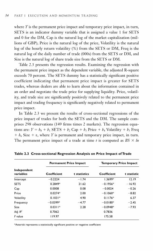
where Y is the permanent price impact and temporary price impact, in turn,SETS is an indicator dummy variable that is assigned a value 1 for SETSand 0 for the DM, Cap is the natural log of the market capitalization (mil-lions of GBP), Price is the natural log of the price, Volatility is the naturallog of the hourly return volatility (%) from the SETS or DM, Freq is thenatural log of the daily number of trade (000s) from the SETS or DM, andSize is the natural log of share trade size from the SETS or DM.
Table 2.3 presents the regression results. Examining the regression withthe permanent price impact as the dependent variable, the adjusted R-squareexceeds 70 percent. The SETS dummy has a statistically significant positivecoefficient indicating that permanent price impact is greater for SETStrades, whereas dealers are able to learn about the information contained inan order and negotiate the trade price for supplying liquidity. Price, volatil-ity, and trade size are significantly positively related to the permanent priceimpact and trading frequency is significantly negatively related to permanentprice impact.
In Table 2.3 we present the results of cross-sectional regressions of theprice impact of trades for both the SETS and the DM. The sample com-prises 298 observations (149 firms times 2 markets). The regression equa-tions are: Y b0 b1 SETS b2 Cap b3 Price b4 Volatility b5 Freq b6 Size ε, where Y is permanent and temporary price impact, in turn.The permanent price impact of a trade at time t is computed as BS ln
34 Part i EXECUTION A ND MOMENTUM TR ADING
Table 2.3 Cross-sectional Regression Analysis on Price Impact of Trade
Permanent Price Impact Temporary Price Impact
Independentvariables Coefficient t statistics Coefficient t statistic
Intercept 0.2224 1.74 1.3699* 12.19
SETS 0.2849* 21.62 0.1956* 16.92
Cap 0.0008 0.08 0.0024 0.26
Price 0.0274* 2.00 0.1060* 8.82
Volatility 0.1031* 4.90 0.1176* 6.37
Frequency 0.0399* 4.77 0.0180* 2.45
Size 0.0311* 2.28 0.0948* 7.93
Adj. R2 0.7062 0.7836
F value 119.97 175.58
*Asterisk represents a statistically significant positive or negative coefficient

(PA/PB) 100 where BS equals plus (minus) one for buyer (seller) initiatedtrade and if a trade occurs at time t, designate the price of that trade as PT,the price of the third subsequent trade as PA and the price of the twelfthprevious trade as PB. The temporary price impact of a trade at time t iscomputed as BS ln (PT/PA) 100. SETS is a dummy variable thatequals 1 if the observation is aggregated from the SETS market. Cap is thenatural log of the market capitalization (millions). Price is the natural log ofthe price. Volatility is the natural log of the hourly return volatility (%)from the SETS or DM. Freq is the natural log of the daily number of trade(000s) from the SETS or DM. Size is the natural log of share trade sizefrom the SETS or DM.
Examining the regressions with the temporary price impact as thedependent variable, the adjusted R-square is 78 percent. The SETSdummy has a statistically significant negative coefficient indicating that theliquidity is cheaper on SETS and costly on the DM. However, not alltrades will automatically gravitate to SETS because total price impact islower on DM markets for larger trade sizes. Moreover, large trades maysimply be impossible to execute on SETS. Temporary price impact is lowerfor firms with a higher price, more frequent trading, and larger-sizedtrades. But higher volatility is associated with an increase in the temporaryprice impact of trades.
Regression results in Table 2.3 are consistent with those presented inTable 2.2 for SETS versus dealer comparisons as well as trade size compar-isons. Coefficients for the control variables are also consistent with previousmicrostructure literature such as Stoll (2000).
Qualitatively similar results in terms of adjusted R-squares, and direc-tion, magnitude, and statistical significance of coefficients are obtainedwhen we estimate Equation 2.4 separately for the SETS and DM and,therefore, these results are not reported in tables for brevity.
CONCLUSION
We examine trading on the London Stock Exchange where the same stocksare traded on a computer-based trading system called SETS and on a DM.Dealers have no obligations to post quotes or to support the market in anyway. We find that the SETS market has more trades overall, but the tradesare larger on the DM and the DM dominates very large sized trades.
chapter 2 Informed Trading in Parallel markets 35
We find significantly greater permanent price impact on SETS com-pared with the DM for both the overall sample and for each size category.Consequently, we believe that the informed trades are routed to SETSwhile the DM is able to effectively identify informed trades ex-ante. Suchidentification of trade motives enables dealers to either screen out theinformed trades, avoiding losses, or trade effectively with them. In theprocess, dealers learn information useful for their own trading.
Further, we find that the temporary price impact on the SETS market isless than on the DM. However, we note that only small quantities aretraded on SETS so the temporary price impact could be large on SETS ifan order marched up the book. For larger trades, liquidity can be purchasedon the DM at a premium. Premiums paid to the dealers are justified if theyare less than the cost of marching up or down the order book to executelarge quantities. A multivariate investigation shows that our findings ofhigher permanent and lower temporary price impacts on SETS hold afterwe control for firm and trading characteristics.
ACKNOWLEDGMENTS
We thank Andrew Ellul and participants at the 14th Annual Conference on Financial Economics, 2003, for useful comments. Any errors remain our own.
REFERENCES
Barclay, M.J., Hendershott, T., and McCormick, D.T. (2003) CompetitionAmong Trading Venues: Information and Trading in ECNs. Journal ofFinance, 58(6): 2637–2665.
Bernhardt, D. and Dvoracek, V., Hughson, E., and Werner, I. (2005) WhyDo Larger Orders Receive Discounts on the London Stock Exchange?Review of Financial Studies, 18(4): 1343–1368.
Board, J. and Wells S. (2001) Liquidity and Best Execution in the UK: A Comparison of SETS and Tradepoint. Journal of Asset Management,1(4): 344–365.
Booth, G., Lin, J., Martikainen, T., and Tse, Y. (2002) Trading and Pricingin Upstairs and Downstairs Stock Markets. Review of Financial Studies,15(4): 1111–1135.
36 Part i EXECUTION A ND MOMENTUM TR ADING

Chowdhry, B. and Nanda, V. (1991) Multi-Market Trading and MarketLiquidity. Review of Financial Studies, 4(3): 483–511.
Easley, D., Kiefer, N., and O’Hara, M. (1996) Cream-Skimming or ProfitSharing? The Curious Role of Purchased Order Flow. Journal ofFinance, 51(3): 811–833.
Easley, D. and O’Hara, M. (1987) Price, Trade Size, and Information inSecurities Markets. Journal of Financial Economics, 19(1): 69–90.
Ellul, A., Shin, H., and Tonks, I. (2005) Toward Deep and Liquid Markets:Lesson from the Open and Close at the London Stock Exchange. Journal of Financial and Quantitative Analysis, 40(4): 779–801.
Franke, G., and D. Hess. (2000) Anonymous Electronic Trading VersusFloor Trading. Journal of Empirical Finance. 7(5): 445–478.
Friederich, S. and Payne, R. (2007) Dealer Liquidity in an Auction Market:Evidence from the London Stock Exchange. The Economic Journal,117(522): 1168–1191.
Glosten, L.R. (1994) Is the Electronic Open Limit Order Book Inevitable?Journal of Finance, 49(4): 1127–1161.
Gramming, J., Schiereck, D., and Theissen, E. (2001) Knowing Me, KnowYou: Trader Anonymity and Informed Trading in Parallel Markets.Journal of Financial Markets, 4(4): 385–412.
Grossman, S. (1992) The Information Role of Upstairs and DownstairsMarkets. Journal of Business 65(4): 509–529.
Hansch O., Naik, N.Y., and Viswanathan, S. (1999) Preferencing, Internal-izat ion and Best Execution: Evidence From the London StockExchange. Journal of Finance, 54(5): 1799–1828.
Heidle, H. and Huang, R. (2002) Information-Based Trading in Dealer andAuction Markets: An Analysis of Exchange Listings. Journal of Financialand Quantitative Analysis, 37(3): 391–424.
Keim, B. and Madhavan, A. (1996) The Upstairs Market for Large-BlockTransactions: Analysis and Measurement of Price Effects. Review ofFinancial Studies, 9(1): 1–36.
Madhavan, A. (1995) Consolidation, Fragmentation, and the Disclosure ofTrading Information. Review of Financial Studies, 8(3): 579–603.
Naik, N.Y., Neuberger, A.J., and Viswanathan, S. (1999) Trade DisclosureRegulation in Markets with Negotiated Trades. Review of FinancialStudies, 12(4): 873–900.
chapter 2 Informed Trading in Parallel markets 37

Pagano, M. and Roell, A. (1996) Transparency and Liquidity: A Comparisonof Auction and Dealer Markets with Informed Trading. Journal ofFinance, 51(2): 579–611.
Schwartz, R. and Steil, B. (1996) Equity Trading III: Institutional InvestorTrading Practices and Preferences. In Steil, B. et al. (eds.) The EuropeanEquity Markets. London: Royal Institute of International Affairs.
Seppi, D. (1990) Equilibrium Block Trading and Asymmetric Information.Journal of Finance, 45(1): 73–94.
Smith, B., Turnbull, A., and White, R. (2001) Upstairs Market for Principaland Agency Trades: Analysis of Adverse Information and Price Effects.Journal of Finance, 56(5): 1723–1746.
Stoll, H.R. (2000) Friction. Journal of Finance, 55(4): 1479–1514.
NOTES
1. A few stocks that have been deleted from these indexes continue to betraded on SETS.
2. Of course, participants can disagree on interpretation of commoninformation and thus an informed trader can trade with anotherinformed trader in real world trade settings. Most theory models, how-ever, simplify trades to include either one informed and one liquiditytrader or both liquidity traders.
3. Booth, Lin, Martikainen, and Tse (2002) find insignificant price move-ment five trades before and three trades after trade t.
38 Part i EXECUTION A ND MOMENTUM TR ADING

39
3C H A P T E R
Momentum Tradingfor the PrivateInvestor
Alexander Molchanov and Philip A. Stork
ABSTRACT
This chapter explores the potential profitability of a momentum strategy fora private investor. Such a strategy is based on price continuation and requiresbuying stocks that have performed well in the past while short selling under-performing stocks. In order to replicate a trading strategy readily attainableby individual investors, we only select constituents of major worldwideindexes. Consistent with prior work, we document strong momentum inshares around the world. However, we also find that when trading costs areaccounted for, momentum profits disappear in some markets. Nevertheless,in Australia and Canada, momentum profits remain positive and significant.
INTRODUCTION
Since the seminal paper by Jegadeesh and Titman (1993), who analyzereturns to buying winners and selling losers, the so-called “momentumeffect” has been highlighted by both academics and practitioners alike.1 Themain presumption behind the momentum effect theory is that it is possibleto predict future price movements based on past price trends. More specifi-cally, past winners keep outperforming past losers. The momentum effect isof particular interest to researchers, as it is one of the best documentedchallenges to the efficient market hypothesis which, in its basic form, tells
us that price changes should be unpredictable. While several potentialexplanations for the momentum effect have been proposed, a general con-sensus is yet to be reached.2
The apparent simplicity of a momentum strategy implementation makesit an attractive choice for an individual investor. After all, one only needs torank stocks according to their past performance. This chapter analyzes theprofitability of the momentum strategy for such an investor. The next ques-tion is which shares to select for inclusion in the momentum portfolio. Weselect 220 of the world’s largest shares—constituents of well-known stockindexes. We have two main reasons for making such a choice. First, theseshares are likely to have low transaction costs compared to other stocks.Second, as Barber and Odean (2008) point out, individual investors, whenfaced with a choice of thousands of stocks, tend to select those that catchtheir attention. Index constituents are more likely to do that.
Consistent with prior studies, we document medium-term momentum inall the markets we consider, including those of Western Europe, the UnitedStates, Northern Europe, Australia, and Canada. Additionally, and to nosurprise, once trading costs have been accounted for then some of the prof-its disappear. However, momentum profits in Australia and Canada remainstatistically and economically significant, indicating that following a simplemomentum strategy could potentially generate abnormal returns, even for aprivate investor.
DATA
We use only the largest shares that are traded in some of the most liquidmarkets. For a private investor it is relatively easy to find out which sharesmake up any of the main share indexes available. In these largest shares, aprivate investor will encounter very few, if any, problems when trading.Going short will usually be possible at reasonable costs, as there is amplesupply. Moreover, the available price data will contain only a minimalamount of the distortions that are often found in the share prices of smallerstocks, including bid-ask bounces, unrepresentative prices due to infrequenttrading or other illiquidity related issues.
From Datastream, we download end-of-month return indexes and trad-ing volumes of the constituent shares of five main equity indexes. The sam-ple period runs from December 1991 to January 2008, comprising 193observations in total. We have selected three indexes from Dow Jones &
40 Part i EXECUTION A ND MOMENTUM TR ADING

Company, Inc. (Dow Jones) and two exchange-generated indexes. The firstindex is the Dow Jones EURO STOXX 50, which consists of the 50 stockswith the highest free-float market capitalization of the 600 largest stockstraded on the major exchanges of 18 European countries.3 Second, theDow Jones Industrial Average 30 Index represents large and well-knownU.S. companies. All industries are covered and the components are selectedat the discretion of The Wall Street Journal editors. Third, the Dow JonesSTOXX Nordic 30 provides a blue-chip representation of the super sectorleaders in the Nordic region, covering 30 stocks from Denmark, Finland,Iceland, Norway, and Sweden. The S&P/ASX 50 index places an emphasison liquidity and comprises the 50 largest stocks by market capitalization inAustralia. Finally, the S&P/TSX 60 index is a list of the sixty largest com-panies on the Toronto Stock Exchange in Canada as measured by marketcapitalization. Together, these five indexes comprise 220 of the world’slargest and most liquid stocks. This approach contrasts with other momen-tum studies which usually focus either on all shares listed on a nationalexchange or on a sample of national indexes.
Prior to its announcement, an investor cannot know which shares will beadded or removed from the list of constituents. We have removed thispotential survivorship bias from our sample using proprietary data kindlyprovided to us by Dow Jones. Stepwise, we assess per individual indexwhich shares are added and deleted monthly based on the informationretrieved from Dow Jones and the websites of the two exchanges. We man-ually adjust the lists of constituent shares accordingly. Each monthly list ofconstituent shares that comprise the index thus reflects only the informa-tion available up until that date. This procedure ensures that the survivor-ship bias is removed from the data. Of the five indexes chosen, we wereunable to obtain all additions and deletions for only the S&P/ASX 50 andthe S&P/TSX 60 indexes. We are thus unable to adjust those two indexesprior to January 2000 and therefore some survivorship bias may remain forthe period between 1992 and 1999. We have no reason to believe that thishas significant affects on our results.
MOMENTUM TRADING RESULTS
We execute the following procedure to calculate momentum returns. Theranking period is defined as the period during which returns are calculatedin order to rank the shares according to their relative return levels. The
chapter 3 Momentum Trading for the Private Investor 41

holding period is defined as the period after the ranking period, duringwhich the returns from holding the shares are realized. Every month, for aspecific ranking period, the returns of all shares are calculated and ranked.The top five winners are bought and the bottom five losers are sold short,and we thus hold these 10 shares in position. We initially choose the mini-mum number of shares per long or short portfolio to equal five, as othermomentum trading studies also often use deciles. Furthermore, we belowanalyze the effects of changing this number and show that a reductionincreases the momentum returns generated but at the same time lowers thestatistical reliability of the results.
We vary both the ranking and the holding period between 1 and 12months. We utilize the investment rule that equally weighted momentumstrategies of varying vintages are simultaneously in effect at all times, following Jegadeesh and Titman (1993, 2001) and Griffin, Ji, and Martin(2003). For comparison purposes, we apply the most commonly usedreturn calculation method. We acknowledge that the implicit monthlyrebalancing is potentially oversimplifying and may, in practice, increasetransaction costs, as pointed out by Liu and Strong (2008). Moreover, wefollow the common practice of skipping one month between ranking andholding periods in order to minimize microstructure price distortions. Asa robustness test, we also calculated momentum returns without skippingone month. The results obtained contain few surprises and are broadly inline with, for example, the findings of Griffin, Ji, and Martin (2003), andare available from the authors upon request. For each of the five data sam-ples, the annualized momentum returns are calculated. Table 3.1 reportsthe returns for the highest versus lowest portfolio across several rankingand holding period combinations. Corresponding t values are given inparentheses.
Table 3.1 shows for all five geographical areas that positive momentumreturns are generated for the most commonly used ranking and holdingperiod combinations of 6, 9, and 12 months. Apparently, a sample size of30 to 60 shares suffices to convincingly demonstrate the pervasive pres-ence of momentum effects. For three of the f ive samples (Europe,Nordic, and the United States), the returns are statistically not signifi-cant. For Australia and Canada, the returns are markedly higher and sig-nificant, as confirmed by the t statistics. For these samples, the annualizedreturns range between 20 percent and 30 percent for various ranking andholding periods.
42 Part i EXECUTION A ND MOMENTUM TR ADING

chapter 3 Momentum Trading for the Private Investor 43
Table 3.1 Momentum Returns
Panel A. S&P/ASX 50 (Australia)
Holding Period in Months
1 3 6 9 12
Ranking period 1 7.36%in Months (1.14)
3 13.52% 19.74%(1.82) (3.26)
6 24.09% 24.02% 23.82%(2.99) (3.59) (3.95)
9 31.17% 27.73% 23.71% 20.24%(4.31) (4.03) (3.81) (3.72)
12 29.82% 27.58% 23.98% 20.67% 17.06%(3.82) (3.87) (3.84) (3.65) (3.34)
Panel B. ASX/TSX 60 (Canada)
Holding Period in Months
1 3 6 9 12
Ranking Period 1 1.15%in Months (0.12)
3 0.40% 15.82%(0.03) (1.51)
6 26.46% 24.63% 27.72%(2.13) (2.15) (2.65)
9 31.00% 31.48% 29.34% 24.38%(2.63) (2.77) (2.71) (2.49)
12 29.79% 29.82% 23.37% 20.89% 19.55%(2.40) (2.55) (2.02) (1.87) (1.81)
Panel C. Dow Jones Industrial Average 30
Holding Period in Months
1 3 6 9 12
Ranking Period 1 0.72%in Months (0.13)
3 4.08% 6.24%(0.75) (1.35)
6 3.72% 2.16% 2.16%(0.67) (0.45) (0.50)
9 1.56% 2.88% 5.04% 6.24%(0.22) (0.48) (0.90) (1.11)
12 1.20% 4.08% 6.24% 5.04% 5.16%(0.18) (0.64) (0.96) (0.83) (0.95)
(Continued.)

44 Part i EXECUTION A ND MOMENTUM TR ADING
Panel D. Dow Jones STOXX Nordic 30
Holding Period in Months
1 3 6 9 12
Ranking Period 1 16.80%
in Months (0.85)
3 4.56% 1.80%
(0.44) (0.23)
6 8.76% 10.44% 10.20%
(0.82) (1.12) (1.19)
9 2.64% 7.08% 4.56% 3.60%
(0.26) (0.81) (0.54) (0.47)
12 2.76% 2.88% 5.76% 4.68% 4.44%
(0.28) (0.32) (0.68) (0.58) (0.57)
Panel E. Dow Jones EURO STOXX 50
Holding Period in Months
1 3 6 9 12
Ranking Period 1 6.84%
in Months (0.85)
3 2.04% 5.64%
(0.24) (0.75)
6 1.92% 5.64% 5.64%
(0.22) (0.71) (0.82)
9 5.76% 8.28% 7.44% 7.44%
(0.63) (0.98) (1.00) (1.05)
12 4.68% 6.35% 7.20% 3.72% 3.48%
(0.49) (0.74) (0.89) (0.50) (0.48)
A second observation is that the strength of the momentum effectsdepends on the duration of the ranking and holding period. For theshorter ranking periods of one and three months, the momentum returnsfor several samples turn negative, although the amounts are statisticallyinsignificant. Our finding of lower momentum returns for the short-termranking periods is in line with prior empirical studies; see, for example,Jegadeesh and Titman (2001).
Table 3.1 (Continued)

chapter 3 Momentum Trading for the Private Investor 45C
umul
ativ
e re
turn
in %
-po
ints
Feb-
93
Feb-
94
Feb-
95
Feb-
96
Feb-
97
Feb-
98
Feb-
99
Feb-
00
Feb-
01
Feb-
02
Feb-
03
Feb-
04
Feb-
06
Feb-
05
Feb-
07
Feb-
08
250%
200%
150%
100%
50%
0%
Figure 3.1 Average of All Cumulative Momentum Returns
ROBUSTNESS TESTS
In this section we conduct a number of robustness tests in order to analyzein more detail the behavior of the momentum effect. We commence byanalyzing the behavior of the momentum returns over time. Could it bethat this is a disappearing phenomenon, or is it still present in the mostrecent data? Figure 3.1 shows the average of all five areas’ cumulative (12 6) momentum returns over the full duration of the sample.
The cumulative momentum returns in Figure 3.1 show a continuingupward movement, albeit with several periods of severe volatility. In 2002,for example, the returns strongly increased only to fall again in 2003. Thepeak in cumulative returns of 2002 was not reached again until 2007.Although the volatility of the returns is apparently quite high, the strongpositive trend nevertheless suggests that the momentum effect is still goingstrong in recent years.
However, a further analysis, as seen below, indicates that the above con-clusion is premature and that the true story is more nuanced. Instead ofaveraging out the cumulative returns over the five samples, we now analyzethe results per individual sample. We split the period into two subperiods,namely, 1992 to 1999 and 2000 to 2008. The respective average momen-tum returns are presented in Figure 3.2.

A surprising picture emerges from Figure 3.2. For the first subperiod1992 to 1999, four of the f ive samples generate average momentumreturns in excess of 10 percent. Only in the Nordic sample do themomentum returns remain subdued at a meager 6.10 percent. However,in the second subperiod 2000 to 2008, four of the five samples showmarkedly lower momentum returns. For the Dow Jones Euro STOXX 50and the Dow Jones Industrial Average 30 samples, the returns are lessthan 2 percent and have thus almost totally disappeared. Only in theAustralian sample did the momentum returns increase during the secondsubperiod.
Next, we analyze to what extent the results depend on the number ofshares being used in the trading strategy. In the above calculations we tooka position of five shares long and five shares short, thus a total of 10. Wenow reduce the number of shares in the portfolios. It is of course easierand cheaper to trade fewer shares, but if we do that we can expect moreerratic trading results due to less averaging out of the returns. To ensure
46 Part i EXECUTION A ND MOMENTUM TR ADING
Mo
men
tum
ret
urn
in %
-po
ints
1992-1999 6.10%5.37%
Nordic12.99%0.74%
Euro10.27%1.95%
DJIA13.15%35.28%
Australia29.64%16.83%
Canada
40%
35%
30%
25%
20%
15%
10%
5%
0%
2000-2008
Figure 3.2 Individual Momentum Returns per Subperiod

consistency, we continue to conduct the above-used (12 6) combinationof ranking and holding periods.4
For most samples, the most extreme losers and winners tend to show thestrongest momentum effects, which is in line with the results found inStork (2008). The cumulative momentum returns tend to reduce stepwisefrom the first ranked shares to the f ifth ranked shares. The averagemomentum return is depicted in Figure 3.3. Although the details are notdiscussed here, we find a corresponding decrease in cumulative momentumreturns for most other holding and ranking periods. Our conclusion is thatthe common practice used by momentum studies of dividing the shareswithin the sample in deciles increases the statistical reliability yet, at thesame time, reduces the absolute size of the momentum effect. Raising thenumber of shares in the momentum portfolio reduces both the expectedlevel and volatility of the returns. The investor who utilizes a momentuminvestment strategy in the market faces this tradeoff.
TRADING WITH A VOLUME FILTER
In this section we present the results of applying a simple volume filter tothe positions. Several authors have already linked momentum and tradingvolume. Conrad, Hameed, and Niden (1994) use weekly NASDAQ stockprices between 1983 and 1990 and find that for past losers, high tradingvolumes predict high future returns. For winners, this relationship is lessevident. Momentum returns are higher if low volume losers are sold asopposed to high volume losers.
The change in trading volume is calculated as the last month’s volumedivided by the average volume of the three preceding months. Lee andSwaminathan (2000) show that most of the predictive power of trading vol-ume is attributable to changes in the level of trading activity rather thanlagged volume. This result supports our choice of trading volume measure-ment. We have arbitrarily chosen a length of three months. However, wefind that increasing the length to 6 or 12 months has only marginal impacton our key findings.
We build on the Conrad, Hameed, and Niden (1994) study and filterout those shares for which the trading volume changes more than a spec-ified threshold. We set these filter-limits somewhat arbitrarily in order toensure that volume can neither have increased more than 10 percent nor
chapter 3 Momentum Trading for the Private Investor 47

48 Part i EXECUTION A ND MOMENTUM TR ADING
Table 3.2 Filtered Momentum Returns and Portfolio Size
Number of shares
1 2 3 4 5
S&P/ASX 50 (Australia) 40.88% 41.50% 34.63% 25.38% 25.61%
143 164 181 183 183
(2.44) (2.85) (3.13) (2.87) (3.35)
S&P/TSX 60 (Canada) 30.35% 24.43% 23.52% 15.63% 13.10%
128 162 175 179 181
(1.31) (1.41) (1.80) (1.38) (1.24)
Dow Jones 8.82% 0.22% 12.58% 7.92% 9.56%
Industrial Average 30 124 158 165 178 178
(0.60) (0.02) (1.12) (0.70) (1.03)
Dow Jones 63.56% 18.21% 7.55% 2.66% 1.88%
STOXX Nordic 30 37 69 89 122 132
(1.51) (0.48) (0.2) (0.10) (0.08)
Dow Jones 59.43% 54.55% 22.38% 10.93% 4.74%
EURO STOXX 50 88 119 140 163 166
(1.87) (2.24) (0.99) (0.58) (0.27)
fallen more than 50 percent. Although we find that the filtered momen-tum returns do not depend strongly on the thresholds used in the vol-ume filters, a more detailed sensitivity analysis falls outside the scope ofthis chapter.
In some months, all winners or losers are f iltered out: for thosemonths, the strategy cannot be executed and no momentum return iscalculated. Table 3.2 shows the filtered momentum trading returns, thenumber of monthly returns, and the t statistics in parentheses for the (12 6)-strategy.
Table 3.2 shows an interesting picture. In line with the results in Table 3.1,we find that for most samples the highest filtered returns are generated whenusing only a minimal number of shares. The returns are widely dispersed, rang-ing from a maximum of 64 percent to a minimum of 9 percent. Unsurpris-ingly, the volatility decreases when the portfolio size is augmented. Moreover,use of the volume filter tends to cause the number of observations to decreaseand the returns to become more erratic. As a result, it is difficult to draw anyconsistent conclusions per individual sample. As a next step, we calculate aver-age filtered momentum returns for each portfolio size, which enables us to bet-ter compare the filtered versus unfiltered trading strategy results.

Figure 3.3 shows that for the smaller portfolios the average momentumreturn increases after applying a volume filter. Even though marginal, thedifference for the (relatively) large sizes of four and five shares favors theunfiltered strategy. The highest average momentum returns are apparentlyobtained by applying a volume filter on very small portfolios. These returnsfluctuate wildly and are thus quite risky.
PRIVATE INVESTOR TRADING
Because of its simplicity, the momentum strategy with or without a filtershould in practice be tradable fairly easily and without too many costs. Weassume one-sided trading costs of 0.3 percent and a bid-offer spread of0.3 percent as well. For consistency we continue to focus on the (12 6)-strategy. For ease of exposition we first focus on the smallest portfolioswhich consist of one share long and one share short. We simultaneously buyand sell these two shares and after six months conduct an offsetting trade.
chapter 3 Momentum Trading for the Private Investor 49A
vera
ge m
om
entu
m r
etru
ns
Number of shares used
Unfiltered 21.76%
37.08%
1
18.31%
27.69%
2
17.23%
20.13%
3
14.47%
11.44%
4
13.31%
10.98%
5
40%
35%
30%
25%
20%
15%
10%
5%
0%
Filtered
Figure 3.3 Comparison of Filtered and Unfiltered Trading Strategies
We thus conduct four trades for each portfolio. Per portfolio, this meansthat we pay four times the transaction costs of 0.3 percent and we lose twotimes the bid-offer spread of 0.3 percent for a total of 1.8 percent. These“costs” are incurred per portfolio that is held for six months, thus twice per year, so that the overall trading costs equal 3.6 percent per year. On topof these costs we must add the stock lending fee, usually expressed as a percentage spread of, for example, 1 percent. Finally, we have to pay somemiscellaneous costs for events such as corporate actions, a fixed-account feeand a fee dependent on the number of shares registered with the broker. Intotal, the miscellaneous fees should not exceed 0.4 percent. The total costsamount to around 5 percent per year.
Our cost-estimates are fairly conservative and are likely to be lower inpractice for an experienced and savvy private investor. For example the bid-offer spread in blue chip shares usually is less than 0.3 percent. Moreover, ifsomewhat larger amounts are traded, the trading costs will be lower as well.Finally, we have assumed that each consecutive trading portfolio is differ-ent. In reality, however, shares stay in or out of market favor for prolongedperiods of time. In such scenarios the composition of the portfolio remainsunaltered and the number of trades comes out lower.
If total trading costs amount to around 5 percent, we conclude that forthe period since the year 2000 the unfiltered momentum trading resultsobtainable for the private investor were nil or even negative for the Euro,Nordic, and U.S. areas. In Australia and Canada, however, a private investorcould have made significant momentum profits in excess of 10 percent perannum even after deduction of all costs.
CONCLUSION
The momentum effect—past winners continuing to outperform past los-ers—has been one of the main challenges to the efficient market hypothe-sis. Following a simple strategy of buying past winners and selling pastlosers seems to generate significantly positive abnormal returns in all themarkets we consider in this chapter. Our findings are robust to a number oftests. We confirm that momentum profits do not disappear over time; theyare more pronounced for extreme winners and losers; and they are ampli-fied with an application of a simple volume filter.
We are looking at the viability of the momentum strategy from the per-spective of the private investor who is likely to encounter significant trading
50 Part i EXECUTION A ND MOMENTUM TR ADING

costs. Indeed, consistent with conventional wisdom and academic evidence,once the trading costs are accounted for, some of the momentum profitsdisappear. Nevertheless, these profits remain significant in the Australianand Canadian markets. However, one has to exercise caution in implement-ing such a strategy, as there is no guarantee these profits will repeat them-selves in the future.
ACKNOWLEDGMENTS
We thank Henk Berkman, Glen Boyle, Ben Jacobsen, Ben Marshal, andDavid Reed for helpful comments to earlier versions of this chapter. We aregrateful to Dow Jones Indexes for providing us with their proprietary data.
REFERENCES
Barber, B.M. and Odean, T. (2008) All That Glitters: The Effect of Atten-tion and News on the Buying Behavior of Individual and InstitutionalInvestors. Review of Financial Studies 21(2): 785–818.
Conrad, J.S., Hameed, A., and Niden, C. (1994) Volume and Autocovari-ances in Short-Horizon Individual Security Returns. Journal of Finance,49(4): 1305–1329.
Daniel, K., Hirshleifer, D., and Subramanyam, A. (1998) Investor Psychol-ogy and Market Under- and Overreactions. Journal of Finance, 53(6):1839–1885.
Griffin, J.M., Ji, S., and Martin, S. (2003) Momentum Investing and Busi-ness Cycle Risk: Evidence from Pole to Pole. Journal of Finance, 58(6):2285–2320.
Grundy, B.D. and Martin, J.S. (2001) Understanding the Nature of Risksand the Source of Rewards to Momentum Investing. Review of Finan-cial Studies, 14(1): 29–78.
Hong, H. and Stein, J. (1999) A Unif ied Theory of Underreaction,Momentum Trading, and Overreaction in Asset Markets. Journal ofFinance, 54(6): 2143–2184.
Jegadeesh, N. and Titman, S. (1993) Returns to Buying Winners and Sell-ing Losers: Implications for Stock Market Eff iciency. Journal ofFinance, 48(1): 65–91.
chapter 3 Momentum Trading for the Private Investor 51

Jegadeesh, N. and Titman, S. (2001) Profitability of Momentum Strategies:An Evaluation of Alternative Explanations. Journal of Finance, 56(2):699–720.
Lee, C.M.C. and Swaminathan, B. (2000) Price Momentum and TradingVolume. Journal of Finance, 45(5): 2017–2069.
Liu, W. and Strong, N. (2008) Biases in Decomposing Holding PeriodPortfolio Returns. Review of Financial Studies, 21(5): 2243–2274.
Nijman, T., Swinkels, L., and Verbeek, M. (2004) Do Countries or Indus-tries Explain Momentum in Europe? Journal of Empirical Finance,11(4): 461–481.
Stork, P.A. (2008) Continuing the Momentum. Infinz Journal, September:30–33.
NOTES
1. Other prominent papers documenting momentum in stock returns are,for example, Grundy and Martin (2001) and Nijman, Swinkels, andVerbeek (2004).
2. Daniel, Hirshleifer, and Subramanyam (1998) attribute momentum totraders’ overconfidence; they ascribe the performance of ex-post win-ners to superior stock selection, while ex-post losers are explained bybad luck. Therefore, delayed overreaction will drive the momentumprofits. Hong and Stein (1999) assume that investors use only partialinformation to update their expectations. This will cause short-rununderreactions and long-run overreactions, resulting in momentumprofits.
3. See www.stoxx.com for an overview of the methodology. The markethas chosen this index as one of the standards for exchange-tradedfunds, derivatives, and other European index products.
4. In order to save space we do not tabulate the results; however, they areavailable from the authors upon request.
52 Part i EXECUTION A ND MOMENTUM TR ADING

53
4C H A P T E R
Trading inTurbulent MarketsDoes Momentum Work?
Tim A. Herberger and Daniel M. Kohlert
ABSTRACT
Identifying ways to successfully predict security returns based on pastreturns is a major objective of investment research. One of the most impor-tant strategies, that of momentum (Levy, 1967; Jegadeesh and Titman,1993; Oehler et al., 2003), is employed in this chapter. Using NYSE datafrom December 1994 to May 2009, we analyze whether buying stocks thathave performed well in the past and selling stocks that have performedpoorly in the past can generate significant positive returns, even in a turbu-lent market phase. Our findings suggest that investors using momentumstrategies could have indeed generated superior returns during that timeperiod.
INTRODUCTION
Since it was first reported by Jegadeesh and Titman (1993), the momentumphenomenon has been extensively discussed in the literature. Based on theconcept of “Relative Strength” by Levy (1967), the authors argue that con-trary to the neoclassic efficient market hypothesis, stock prices are auto-correlated. For the U.S. stock market they find that trading strategies thatbuy stocks which have performed well in the past and sell stocks that haveperformed poorly in the past can achieve abnormal market-adjusted returnsthat could not exist if the market was efficient. After Jegadeesh and Titman(1993), many studies tried to reproduce their results by testing momentuminvestment strategies in other stock markets: For example, Rouwenhorst
(1998) shows that momentum can be found in a sample of 12 Europeanstock markets. Chui, Titman, and Wei (2000) confirm momentum for eightAsian stock markets (without Japan), and Glaser and Weber (2003) showthat investment strategies based on momentum can be profitable in theGerman stock market. In an experimental study, Oehler et al. (2003) iden-tify momentum traders and disposition investors.
This chapter uses NYSE data from December 1994 to May 2009 toexamine whether momentum can still be found on the U.S. stock market.This is particularly interesting as the sample period covers extreme marketmoves resulting from the rise and fall of dot-com stocks at the beginning ofthis century and from the current financial crisis. We find significant posi-tive abnormal returns on a market-adjusted basis for a short-term strategywith equally long ranking and holding periods of 3 months as well as for amedium-term strategy based on 6-month-long ranking and holding periods.This holds true even after transaction costs are considered. A long-termstrategy based on 12-month-long ranking and holding periods, however,does not produce significant abnormal returns.
The chapter is organized as follows. The second section of this chapterprovides a literature review, and in the third section we explain thedataset and introduce the methodology adopted. The presentation of theempirical results follows in this chapter’s fourth section, and the fifth sec-tion concludes.
LITERATURE REVIEW
Although the profitability of momentum strategies is rarely disputed, thereis still a great deal of controversy over the reasons for such abnormalreturns. Neoclassical economists attempt to explain momentum as arational compensation for risk, a liquidity premium and /or an illusioninduced by market frictions (Fuertes, Miffre, and Tan, 2009). Lesmond,Schill, and Zhou (2004), for instance, argue that momentum cannot be profitably exploited when transaction costs are considered. Korajczykand Sadka (2004), however, find that transaction costs can only partiallyexplain the profits of momentum strategies. Conrad and Kaul (1998)argued that cross-sectional variation can potentially explain the profitabilityof momentum strategies, and Moskowitz and Grinblatt (1999) find that it isfor the most part attributable to momentum in different industries. Aftercontrolling for momentum across industries, the authors hardly find a profit
54 Part i EXECUTION A ND MOMENTUM TR ADING

in individual stock returns. Another explanation is offered by Wu (2002)and Wang (2003) who assume that the profitability of momentum trading isa result of time-variation in expected returns. Grundy and Martin (2001) and Karolyi and Kho (2004) show, however, that neither industry effects,time-variation in expected returns, nor cross-sectional disparities are themain reasons for the momentum effect and that these factors can explain itonly partially. Also, while Chordia and Shivakumar (2002) indicate thatsome macroeconomic variables (e.g., the yield on a three-month T-bill)predict the momentum phenomenon and the associated payoffs, Griffin, Ji,and Martin (2003) show that this approach also offers an only incompleteexplanation.
Behavioral economists follow another approach. They argue thatmomentum is a consequence of cognitive biases and/or limits to arbitrage.In the model of Barberis, Shleifer, and Vishny (1998), momentum resultsfrom conservatism while representativeness leads to overvaluation and con-sequently to price correction. Daniel, Hirshleifer, and Subrahmanyam(1998) argue that biased self-attribution and overconfidence are the reasonsfor the predictability of equity returns. Chan, Jegadeesh, and Lakonishok(1996) as well as Hong and Stein (1999) attributed momentum to an onlygradual distribution of new information on the market.1 Chui, Titman, andWei (2009) find indications in their analysis of 55 countries that culturaldifferences affect stock return patterns and the extent of the success ofmomentum trading. They argue that individuals from different countriesrespond differently to risk. Hwang and Rubesam (2008), however, note thatat least for the U.S. stock market momentum profits have slowly erodedsince the early 1990s.
DATA AND METHODOLOGY
Monthly stock prices over the period December 31, 1994 to May 31, 2009are obtained from Datastream for all common stocks listed on the NYSE,excluding American depository receipts (ADRs), real estate investment trusts(REITs), closed-end funds, and companies which were delisted during theevaluation period. For our analysis we use returns adjusted for capital gainsand dividends. An equally weighted NYSE Index that consists of all shares ofthe dataset is used as a market proxy. The momentum strategy is intended asa zero-cost portfolio strategy that buys stocks that have performed well in thepast and sells stocks that have performed poorly in the past.
chapter 4 Trading in Turbulent Markets 55

We basically follow the methodology of Jegadeesh and Titman (1993). Wecouch everything in terms of raw returns, and we equally weight these returns.However, in contrast to Jegadeesh and Titman (1993), we do not analyze 16 butthree trading strategies: we use a short-term strategy with a ranking period J of3 months and an equal holding period K ( J 3/K 3), a medium-term strat-egy consisting of a 6-month ranking period as well as a 6-month holdingperiod ( J 6/K 6), and a long-term strategy with a ranking period of12 months and a holding period of 12 months ( J 12/K 12). To increasethe power of our tests, we construct overlapping test runs like Moskowitz andGrinblatt (1999), Jegadeesh and Titman (2001), and Fuertes, Miffre, and Tan(2009). This results in 167 test runs for the 3/3 trading strategy, 161 test runsfor the 6/6 strategy, and 149 test runs for the 12/12 strategy. While Jagadeeshand Titman (1993) sort stocks into 10 deciles according to past performance,and then measure the return differential of the most extreme deciles whichthey denote by P10 – P1, we place even more emphasis on the tails of the per-formance distribution.
One month after the ranking takes place, we sort our sample into onlytwo parts based on past performance: P1, which includes the worst-per-forming 1 percent, and P2, which includes the best-performing 1 percent ofNYSE stocks in the ranking period. Our basic measure of momentum isthen P2 – P1. The top 1 percent portfolio is the winners’ portfolio and thebottom 1 percent portfolio is the losers’ portfolio. The stocks in the indi-vidual portfolios are equally weighted. Contrast to Jegadeesh and Titman(1993), Jegadeesh and Titman (2001), and most former studies, the twoextreme portfolios are formed in order to maximize performance and tominimize transaction costs. This, however, implies fewer diversificationbenefits in the portfolios. In order to avoid biases because of low-pricedstocks, which are documented for example in Conrad and Kaul (1993), par-ticularly for January, we follow the method of Jegadeesh and Titman (2001)and Fuertes, Miffre, and Tan (2009) by (temporarily) excluding stockswhich are priced below $5 at the end of the ranking period.
By skipping a month between the end of the ranking period and thebeginning of the holding period like Rouwenhorst (1998), we avoid someof the bid-ask spread, price pressure, and lagged effects, which could skewour results. These effects are documented for example in Jegadeesh(1990) and Lehmann (1990). The gross return of a test run (cumulativereturn of a holding period of T months in test run i, CRi,T) is defined asfollows:
56 Part i EXECUTION A ND MOMENTUM TR ADING
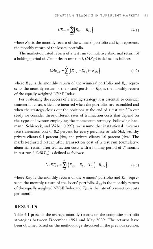
(4.1)
where RW,t is the monthly return of the winners’ portfolio and RL,t representsthe monthly return of the losers’ portfolio.
The market-adjusted return of a test run (cumulative abnormal return ofa holding period of T months in test run i, CARi,T) is defined as follows:
(4.2)
where RW,t is the monthly return of the winners’ portfolio and RL,t repre-sents the monthly return of the losers’ portfolio. RM,t is the monthly returnof the equally weighted NYSE Index.
For evaluating the success of a trading strategy it is essential to considertransaction costs, which are incurred when the portfolios are assembled andwhen the strategy closes out the positions at the end of a test run.2 In ourstudy we consider three different rates of transaction costs that depend onthe type of investor employing the momentum strategy. Following Bro-mann, Schiereck, and Weber (1997), we assume that institutional investorsface transaction cost of 0.2 percent for every purchase or sale (4x), wealthyprivate clients 0.5 percent (4x), and private clients 1.0 percent (4x).3 Themarket-adjusted return after transaction cost of a test run (cumulativeabnormal return after transaction costs with a holding period of T monthsin test run i, CARTi,t) is defined as follows:
(4.3)
where RW, t is the monthly return of the winners’ portfolio and RL,t repre-sents the monthly return of the losers’ portfolio. Rm,t is the monthly returnof the equally weighted NYSE Index and TC,t is the rate of transaction costsper month.
RESULTS
Table 4.1 presents the average monthly returns on the composite portfoliostrategies between December 1994 and May 2009. The returns have been obtained based on the methodology discussed in the previous section.
chapter 4 Trading in Turbulent Markets 57
CR R Ri T W t L tt
T
, , ,= −⎡⎣ ⎤⎦=
∑0
CAR R R Ri T W t L t M tt
T
, , , ,= −( ) −⎡⎣ ⎤⎦=
∑0
CART R R T Ri T Wt L t C t M tt
T
, , , , ,= − −( ) −⎡⎣
⎤⎦
=
∑0
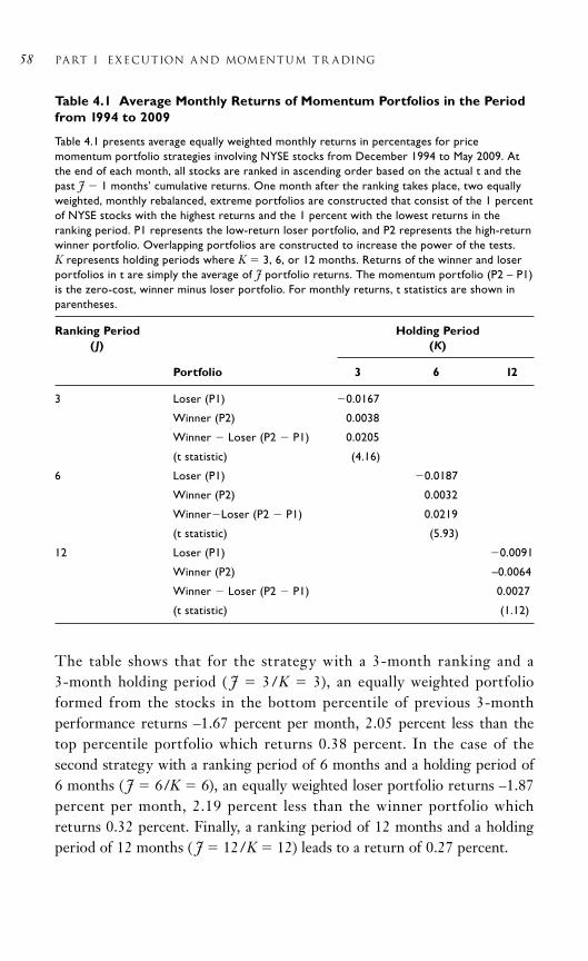
The table shows that for the strategy with a 3-month ranking and a 3-month holding period ( J 3 /K 3), an equally weighted portfolioformed from the stocks in the bottom percentile of previous 3-month performance returns –1.67 percent per month, 2.05 percent less than thetop percentile portfolio which returns 0.38 percent. In the case of the second strategy with a ranking period of 6 months and a holding period of6 months ( J 6/K 6), an equally weighted loser portfolio returns –1.87percent per month, 2.19 percent less than the winner portfolio whichreturns 0.32 percent. Finally, a ranking period of 12 months and a holdingperiod of 12 months ( J 12/K 12) leads to a return of 0.27 percent.
58 Part i EXECUTION A ND MOMENTUM TR ADING
Table 4.1 Average Monthly Returns of Momentum Portfolios in the Periodfrom 1994 to 2009
Table 4.1 presents average equally weighted monthly returns in percentages for pricemomentum portfolio strategies involving NYSE stocks from December 1994 to May 2009. Atthe end of each month, all stocks are ranked in ascending order based on the actual t and thepast J 1 months’ cumulative returns. One month after the ranking takes place, two equallyweighted, monthly rebalanced, extreme portfolios are constructed that consist of the 1 percentof NYSE stocks with the highest returns and the 1 percent with the lowest returns in theranking period. P1 represents the low-return loser portfolio, and P2 represents the high-returnwinner portfolio. Overlapping portfolios are constructed to increase the power of the tests. K represents holding periods where K 3, 6, or 12 months. Returns of the winner and loserportfolios in t are simply the average of J portfolio returns. The momentum portfolio (P2 – P1)is the zero-cost, winner minus loser portfolio. For monthly returns, t statistics are shown inparentheses.
Ranking Period Holding Period(J) (K)
Portfolio 3 6 12
3 Loser (P1) 0.0167
Winner (P2) 0.0038
Winner Loser (P2 P1) 0.0205
(t statistic) (4.16)
6 Loser (P1) 0.0187
Winner (P2) 0.0032
WinnerLoser (P2 P1) 0.0219
(t statistic) (5.93)
12 Loser (P1) 0.0091
Winner (P2) –0.0064
Winner Loser (P2 P1) 0.0027
(t statistic) (1.12)

In this case, an equally weighted portfolio formed from the stocks in thebottom percent of previous three-month performance returns –0.91 percentper month, while the top percent portfolio returns –0.61 percent. Averageoverall returns are highest for the medium-term strategy. This supports theapproach in the literature to mainly focus on this strategy based on 6-monthranking and holding periods (e.g., Jegadeesh and Titman, 1993; Rouwenhorst,1998; Hong, Lim, and Stein, 2000). The winners of the short-term strategyhave much higher returns than the losers. For both the short-term and themedium-term strategy, returns are significant at the 1 percent level. For thelong-term strategy, both winner and loser returns are negative, very close toeach other, and not significant.
Compared with previous findings in the literature, the negative returnsof the loser portfolios are relatively high. Jegadeesh and Titman (1993),Jegadeesh and Titman (2001), Rouwenhorst (1998), and Hong, Lim, andStein (2000), for example, do not find negative returns for their loser port-folios at all. However, these authors report considerably higher averagereturns of their winners’ portfolios. As for our data the difference betweenwinner and loser portfolios is still greater, we find a higher overall perfor-mance of our momentum portfolios. Besides the effect of a potential sur-vivorship bias due to the omission of delisted stocks, a reason for thehigher returns we find is likely to be that we chose smaller and moreextreme portfolios and through this exchanged higher returns for higherrisk by foregoing diversification benefits. As Rouwenhorst (1998) aptlystates, stocks with higher standard deviations, all else equal, are more likelyto show unusual performance.
Looking at the risk of the three momentum portfolios, we find that thestandard deviations decrease with the time horizon of the strategies. Whilethe short-term portfolio has a monthly standard deviation of 6.06 percent,the medium-term portfolio’s standard deviation is 4.33 percent, and thelong-term portfolio’s standard deviation is 3.02 percent. Interestingly, themedium-term strategy has a higher return and simultaneously a lower stan-dard deviation than the short-term strategy. Although the lower standarddeviation of the long-term strategy comes along with a lower return, asexpected, the relationship between risk and return is worst in this case.Compared with Rouwenhorst (1998) who reports monthly standard devia-tions of 5.62 percent for his loser (decile) portfolio, and of 5.27 percent forhis winner (decile) portfolio for the momentum strategy based on 6-month
chapter 4 Trading in Turbulent Markets 59

ranking and holding periods, our standard deviations, which result fromportfolios that contain only the top and bottom 1 percent of availablestocks, do not seem overly high. A further reason for the high returns ofthe strategy may be the particular characteristics of the time period from1994 to 2009 that we are looking at. With the dot-com bubble at the begin-ning of the twentieth century as well as with the financial crisis the marketfaced two strong as well as prolonged declines which should at least partlybe responsible for the highly negative returns of the loser portfolios and theonly slightly positive returns of the winner portfolios.
Table 4.2 presents the average monthly abnormal returns of the momen-tum portfolios using the average monthly NYSE return as the marketproxy. The returns have been obtained based on the methodology discussedin section two. Panel A shows the returns of the market proxy as adjustedto the respective strategy, the raw return of the momentum portfolios, andthe abnormal returns resulting from subtracting market from momentumreturns. As expected based on the results of Table 4.1, the average monthlyabnormal return is highest for the medium-term strategy with 2.08 percent.The abnormal return of the short-term strategy is also considerably highwith 1.83 percent. Both returns are significant at the 1 percent level. Thelong-term strategy produces the lowest and nonsignificant abnormal returnof 0.01 percent.
Assessing the profitability of momentum trading strategies requires anassessment of the trading costs. Panel B therefore shows average monthlyreturns that have been adjusted for a 0.2 percent transaction costs rate.While the short-term strategy’s average monthly abnormal return is 1.56 percent, the medium-term strategy returns 1.95 percent, and thelong-term strategy 0.03 percent. Again, both returns of the short-term aswell as the medium-term strategies are significant at the 1 percent level.Panel C shows average monthly abnormal returns that have been adjustedfor a 0.5 percent transaction costs rate. In this case, the short-term strat-egy’s average monthly abnormal return is 1.40 percent and it is significantat the 1 percent level. The medium-term strategy returns 2.10 percent inexcess of the market. The return is significant at the 1 percent level. Thelong-term strategy is characterized by an insignificant abnormal return of0.02 percent.
In Panel D, transaction costs are increased to 1 percent. Although theshort-term strategy still returns 0.45 percent in excess of the market, thisreturn is no longer significant. The long-term strategy now underperforms
60 Part i EXECUTION A ND MOMENTUM TR ADING

Table 4.2 Abnormal Montly Returns of Momentum Portfolios Using the Average NYSE Return as the Market Proxy overthe Time Period from 1994 until 2009
This table presents average monthly abnormal returns in percentages for price momentum portfolio strategies involving NYSE stocks from December 1994to May 2009. P represents the return of the momentum portfolio, i.e., the zero-cost, winner minus loser portfolio, for a given J/K-strategy. J representsranking periods, where J 3, 6, or 12 months, and K represents holding periods where K 3, 6, or 12 months. M represents the average NYSE returnwhich is used as the market proxy. The abnormal return of the momentum portfolios using the average NYSE return as the market proxy (P – M) iscalculated by subtracting market return from momentum return. In Panel A, raw returns are presented without considering transaction costs. In Panel B,transaction costs of 0.2 percent are considered in calculating the return of the momentum portfolio. In Panel C, transaction costs of 0.5 percent areconsidered in calculating the return of the momentum portfolio. In Panel D, transaction costs of 1 percent are considered in calculating the return of themomentum portfolio. For monthly return differences, t statistics are shown in parentheses.
Panel A Panel B Panel C Panel D
Ranking Period (J) Holding Period (K) Holding Period (K) Holding Period (K) Holding Period (K)
3 6 12 3 6 12 3 6 12 3 6 12
3 Market Return (M) 0.0026 0.0026 0.0026 0.0026
Momentum Return (P) 0.0209 0.0181 0.0140 0.0071
Abnormal Return (P - M) 0.0183 0.0156 0.0114 0.0045
(t-stat) (-3.31) (-2.82) (-2.08) (-0.82)
6 Market Return (M) 0.0015 0.0015 0.0015 0.0015
Momentum Return (P) 0.0223 0.0210 0.0189 0.0154
Abnormal Return (P - M) 0.0208 0.0195 0.0174 0.0139
(t-stat) (-5.10) (-4.77) (-4.27) (-3.41)
12 Market Return (M) 0.0021 0.0021 0.0021 0.0021
Momentum Return (P) 0.0030 0.0023 0.0013 0.0004
Abnormal Return (P - M) 0.0009 0.0002 0.0008 0.0025
(t-stat) (-0.30) (-0.07) (0.28) (0.87)
61

the market by 0.25 percent. Only the medium-term strategy significantlyoutperforms the market at the 1 percent level with an abnormal return of1.39 percent. In general, these returns show that the momentum effect notonly existed in the period we observed, but also that it could have beenprofitably exploited even after considering transaction costs. This at leastapplies to the investor who is willing to bear the considerable risk of usingthis strategy based on the very extremes of the considered stocks’ returndistribution.
This table presents average monthly abnormal returns in percentages for price momentum portfolio strategies involving NYSE stocks fromDecember 1994 to May 2009. P represents the return of the momentumportfolio, i.e., the zero-cost, winner minus loser portfolio, for a given J/K-strategy. J represents ranking periods, where J 3, 6, or 12 months, and Krepresents holding periods where K 3, 6, or 12 months. M represents theaverage NYSE return which is used as the market proxy. The abnormalreturn of the momentum portfolios using the average NYSE return as themarket proxy (P – M) is calculated by subtracting market return frommomentum return. In Panel A, raw returns are presented without consider-ing transaction costs. In Panel B, transaction costs of 0.2 percent are consid-ered in calculating the return of the momentum portfolio. In Panel C,transaction costs of 0.5 percent are considered in calculating the return ofthe momentum portfolio. In Panel D, transaction costs of 1 percent are con-sidered in calculating the return of the momentum portfolio. For monthlyreturn differences, t statistics are shown in parentheses.
CONCLUSION
Using NYSE data from December 1994 to May 2009, we analyze whethermomentum trading strategies can generate significant positive returns evenin a turbulent market phase. Our findings suggest that even after years ofacademic analysis and considerable awareness of momentum effects investorscan still generate superior returns using momentum portfolio strategies. Wefind significant positive abnormal market-adjusted returns for short- andmedium-term momentum strategies based on equally long ranking and for-mation periods of 3 and 6 months, respectively. A long-term strategy basedon equally long ranking and formation periods of 12 months, however, can-not significantly outperform the market. Even after considering transaction
62 Part i EXECUTION A ND MOMENTUM TR ADING

costs of 0.2, 0.5, and 1 percent, respectively, there are significant results.Only the medium-term strategy based on 6-month ranking and holdingperiods, however, significantly outperforms the market if transaction costsare set to 1 percent. Interestingly, the strategy based on 6-month rankingand holding periods offers the highest return while simultaneously havingthe lowest risk in terms of standard deviation.
REFERENCES
Barberis, N., Shleifer, A., and Vishny, R. (1998) A Model of Investor Senti-ment. Journal of Financial Economics, 49(3): 307–343.
Broman, O., Schiereck, D., and Weber, M. (1997) Reichtum durch(A nti )zyklische Handelsstrategien am Deutschen Aktienmarkt.Zeitschrift Für Betriebswirtschaftliche Forschung, 49(7/8): 603–616.
Chan, L., Jegadeesh, N., and Lakonishok, J. (1996) Momentum Strategies.Journal of Finance, 51(5): 1681–1713.
Chordia, T. and Shivakumar, L. (2002) Momentum, Business Cycle, andTime-varying Expected Returns. Journal of Finance, 57(2): 985–1019.
Chui, A., Titman, S. and Wei, J. (2000) Momentum, Legal Systems andOwnership Structure: An Analysis of Asian Stock Markets. Workingpaper, University of Texas, Austin, Texas.
Chui, A., Titman, S. and Wei, J. (2009) Individualism and MomentumAround the World. Available at: http://papers.ssrn.com/sol3/papers.cfm?abstract_id1150076
Conrad, J. and Kaul, G. (1993) Long-term Overreaction or Biases in Com-puted Returns? Journal of Finance, 48(1): 39–63.
Conrad, J. and Kaul, G. (1998) An Anatomy of Trading Strategies. Reviewof Financial Studies, 11(3): 489–519.
Daniel, K., Hirshleifer, D., and Subrahmanyam, A. (1998) Investor Psychol-ogy and Security Market Under- and Overreaction. Journal of Finance,53(6): 1839–1885.
Fuertes, A.-M., Miffre, J., and Tan, W.-H (2009) Momentum Profits, Non-normality Risks and the Business Cycle. Applied Financial Economics,19(12): 935–353.
chapter 4 Trading in Turbulent Markets 63
Glaser, M. and Weber, M. (2003) Momentum and Turnover: EvidenceFrom the German Stock Market. Schmalenbach Business Review, 55(2):108–135.
Griffin, J., Ji, X., and Martin, S. (2003) Momentum Investing and BusinessCycle Risk: Evidence From Pole to Pole. Journal of Finance, 58(6):2515–2547.
Grundy, B. and Martin, S. (2001) Understanding the Nature of the Risksand the Source of the Rewards to Momentum Investing. Review ofFinancial Studies, 14(1): 29–78.
Hong, H., Lim, T., and Stein, J. (2000) Bad News Travels Slowly: Size,Analyst Coverage, and the Profitability of Momentum Strategies. Jour-nal of Finance, 55(1): 265–295.
Hong, H. and Stein, J. (1999) A Unif ied Theory of Underreaction,Momentum Trading, and Overreaction in Asset Markets. Journal ofFinance, 54(6): 2143–2184.
Hwang, S. and Rubesam, A. (2008) The Disappearance of Momentum.Available at: http://preprodpapers.ssrn.com/sol3/papers.cfm?abstract_id968176&rec1&srcabs924522
Jegadeesh, N. (1990) Evidence of Predictable Behaviour of SecurityReturns. Journal of Finance, 45(3): 881–898.
Jegadeesh, N. and Titman, S. (1993) Returns to Buying Winners and Sell-ing Losers: Implication for Stock Market Efficiency. Journal of Finance,48(1): 65–91.
Jegadeesh, N. and Titman, S. (2001) Profitability of Momentum Strategies:An Evaluation of Alternative Explanations. Journal of Finance, 56(2):699–720.
Karolyi, G. and Kho, B. (2004) Momentum Strategies: Some BootstrapTests. Journal of Empirical Finance, 11(1): 509–536.
Korajczyk, R. and Sadka, R. (2004) Are Momentum Profits Robust toTrading Costs. Journal of Finance, 59(3): 1039–1082.
Lehmann, B. (1990) Fads, Martingales and Market Efficiency. QuarterlyJournal of Economics, 105(1): 1–28.
Lesmond, D., Schill, M., and Zhou, C. (2004) The Illusory Nature ofMomentum Profits. Journal of Financial Economics, 71(2): 349–380.
64 Part i EXECUTION A ND MOMENTUM TR ADING

Levy, R. (1967) Relative Strength as a Criterion for Investment Selection.Journal of Finance, 22(4): 595–610.
Moskowitz, T. and Grinblatt, M (1999) Do Industries Explain Momentum?Journal of Finance, 54(4): 1249–1290.
Oehler, A. (2002) Behavioral Finance, Verhaltenswissenschaftliche Finanz-marktforschung und Portfoliomanagement. In: Kleeberg, J. andRehkugler, H. (eds.), Handbuch des Portfolio-management. Bad Soden,Germany: Uhlenbruch-Verlag.
Oehler, A., Heilmann, K., Läger, V., and Oberländer, M. (2003) Coexistenceof Disposition Investors and Momentum Traders in Stock Markets:Experimental Evidence. Journal of International Financial Markets, Insti-tutions & Money, 13(5): 503–524.
Rouwenhorst, G. (1998) International Momentum Strategies. Journal ofFinance, 53(1): 267–284.
Wang, K. (2003) Asset Pricing with Conditioning Information: A NewTest. Journal of Finance, 58(1): 161–195.
Wu, X. (2002) A Conditional Multifactor Analysis of Return Momentum.Journal of Banking and Finance, 26(8): 1675–1696.
NOTES
1. For an explanation of the gradual distribution of new information inthe market, see Oehler (2002).
2. For an overview of the components of trading costs, see Korajczyk andSadka (2004).
3. These assumptions can be considered conservative as transaction costshave decreased since these articles were published due to factors such astechnological change and increased competition.
chapter 4 Trading in Turbulent Markets 65

This page intentionally left blank

67
5C H A P T E R
The FinancialFutures Momentum
Juan Ayora and Hipòlit Torró
ABSTRACT
The momentum strategy is the most famous anomaly arguing against thehypothesis of financial market efficiency. In this chapter, the momentumstrategy produces a significant abnormal return for holding periods of sixmonths and one year using financial futures (stock indexes, currencies, andfixed income). Furthermore, this study characterizes those futures con-tracts that contribute to the momentum strategy return. When the sampleis split in two groups, depending on the level of volatility, a significantlyhigher return is obtained in the high volatility group. Moreover, when thesample of futures is split in four groups, depending on the trading volumeand open interest levels, those contracts with high trading volume and lowopen interest report the best momentum performance.
INTRODUCTION
In recent years a large number of studies have analyzed several investingstrategies that produce abnormal returns in financial markets. As a result,the efficiency of these markets has been again questioned, especially aftermany hedge funds put these strategies into practice. The momentum effectis one of the most important phenomena studied in the literature. Thiseffect is based on the hypothesis that those assets with the best (worst)return performance in the past will continue to perform similarly (best orworst) in the future. The trading rule to exploit this return pattern is very

simple: take long positions in those assets with the best performance in thepast and short positions in those assets with the worst past performances.The momentum effect has been found to be significant for investment hori-zons of between nine months and a year. There is no agreement about anexplanation for the momentum effect. The most important line of worktries to relate the momentum effect strategy return with macroeconomicvariables. This line of work produces quite successful results, and someauthors assert that this phenomenon is compatible with the efficiencyhypothesis—when returns are properly adjusted by risk.
In this chapter, we will study the momentum effect on financial futuresmarkets. This work will contribute to the literature by relating the momen-tum strategy return with liquidity linked variables (trading volume andopen interest) and volatility.
LITERATURE REVIEW
The most important studies covering the momentum effect in stock mar-kets are those of Jegadeesh and Titman (1993, 2001). These authors findsignificant abnormal returns for intermediate investment horizons of up toone year. Recently, Shen, Szakmary, and Sharma (2007), Miffre and Rallis(2007), and Pirrong (2005) found abnormal returns in futures markets forthe momentum strategy. Shen et al. (2007) and Miffre and Rallis (2007)studied the momentum effect in commodity futures markets. Miffre andRallis (2007) concluded that momentum strategies buy backwardated con-tracts and sell contangoed contracts.
The momentum effect survives as the most famous anomaly that arguesagainst the hypothesis of financial market efficiency. There is consensus inthe literature that the profitability of momentum-based trading strategiescannot be fully accounted for in the context of market factor models1. Anoutstanding contribution in this field is made by Karolyi and Kho (2004).These authors propose a very complete bootstrap procedure to test thereturn abnormality in momentum-based strategies. Specifically, they com-pute time-varying expected returns with market-wide and macroeconomicinstrumental variables—and they are able to explain almost 80 percent ofthe profits.
There are few studies relating the momentum effect in futures marketswith open interest, traded volume, and volatility. Bessembinder and Seguin
68 Part i EXECUTION A ND MOMENTUM TR ADING

(1993) make an important contribution in this field. They find a positiverelationship between volatility and traded volume and a negative relation-ship between volatility and open interest. Lee and Swaminathan (2000) usepast traded volume to predict the persistence of the momentum effect instock markets.
DATA
The database used is extracted from a CD published by the CommodityResearch Bureau (CRB). Specifically, we have collected closing prices, tradedvolumes, and open interest. Futures return time-series have been computedwhile carefully avoiding mixing futures contracts with differing maturities.The contracts are rolled over two weeks before the futures maturity.
The sample includes a set of 18 contracts representing the most impor-tant markets in the world.2 The list includes seven currency futures(Euro/USD, Yen/USD, Canadian dollar/USD, British pound/USD, Australian dollar/USD, Swiss franc/USD, and U.S. dollar index); six stockindex futures (CAC 40, FTSE 100, Nikkei 225, S&P 500, Swiss marketindex, Dow Jones EURO STOXX 50); and five fixed income futures (Eurobund 10-Y, Canadian government bond 10-Y, U.S. Treasury note 2-Y, U.S.Treasury note 5-Y, and U.S. Treasury note 10-Y). We have excluded com-modity futures contracts because commodity price time-series have specificspecial features and have been already studied in Shen et al. (2007) andMifre and Rallis (2007). The period for the returns time-series runs fromMay 1991 to December 2007. The time-series of volume and open interestcovers the period January 2001 to December 2007. On average, the trans-action costs of the 18 contracts have been estimated at 0.096 percent overthe average nominal contract values for the studied period. This costincludes the bid-ask spread, and an estimation of the intermediation com-mission for opening and closing futures positions.
METHODOLOGY AND RESULTS
Following the methodology in previous studies such as Shen et al. (2007)and Jegadeesh and Titman (1993, 2001), we have tested the existence of themomentum effect in a sample of futures contracts. We have constructedbasic momentum tests as follows. Firstly, we define five formation periods
chapter 5 The Financial Futures Momentum 69

(F) and five holding periods (H). We have chosen the following periodlengths for F and H: 1, 3, 6, 12, and 24 months. The reported tables willdisplay results only for F H, the remaining combinations of F and Hperiods are omitted to save space. Based on each futures return in the Fperiod, we then group the periods into one of three portfolios (P1, P2, andP3), where P1 contains the six futures with highest past returns (winners);and P3 contains the six futures with lowest past returns (losers). Theremaining six futures are included in the P2 portfolio. We then computeportfolio returns for each holding period. Finally, the momentum portfolioreturn is calculated: P1 – P3. That is, the momentum portfolio containslong positions in the past winning contracts and short positions in the pastlosing contracts.
A momentum effect will exist if the average return of this portfolio ispositive and significantly different from zero. To test the significance ofmomentum profits in each portfolio, we use t statistics that are asymptoti-cally distributed such as N(0,1) under the null hypothesis that the trueprofits are zero. Because we generally use overlapping data, we have cor-rected our standard errors for heteroscedasticity and autocorrelation usingthe Newey and West adjustment.
Momentum Strategy Profits
Table 5.1 presents the results for the whole sample and F E periods. Allthe returns are annualized to facilitate comparison. Two market indicatorsare reported in each row to complete the analysis. The first indicator,termed reference, is an equally weighted portfolio with a long position in each of the 18 contracts in the sample. The second indicator is the S&P 500 index. Results in Table 5.1 show that all the momentum strategiesobtain positive returns: but only for the 6- and 12-month periods are themean returns significantly different to zero at the 5 percent of significancelevel.3 Furthermore, the mean return of momentum strategies for 6 and 12months is more than 500 basic points higher than the reference portfolioand the S&P 500 annual returns. These results are similar to Jagadeesh andTitman (1993 and 2001) for 6- and 12-month periods. Nevertheless, wefound no overreactation evidence in the way De Bondt and Thaler (1985,1987) and Conrad and Kaul (1998) found for the 24-month period in theU.S. stock markets.
70 Part i EXECUTION A ND MOMENTUM TR ADING

Momentum and Volatility
Pirrong (2005) suggests that differences in volatility across futures canmask the momentum effect because highly volatile contracts will be win-ners or losers more frequently than less volatile contracts. Nevertheless,his analysis shows that the momentum effect persists after futures returnsare standardized by their own volatility. We will study this point further.We have split the 18 contracts in two groups of nine contracts, accordingto their daily volatility during the sample period. Table 5.2 reports theresults for the nine most volatile (Panel A), and the nine least volatile(Panel B) contracts. Most volatile contracts show positive returns higherthan the corresponding returns appearing in Table 5.1. On the contrary,less volatile contracts show returns significantly below the correspondingreturns appearing in Table 5.1. The only momentum strategy in Table 5.2with an average return significantly different to zero at the 5 percent sig-nificance level is the six-month momentum strategy in Panel A; and it issignificantly higher than the corresponding return in Table 5.1 using the z test (z 3.365).4 Therefore, we can conclude that the momentum effectis more persistent in highly volatile futures contract portfolios.
chapter 5 The Financial Futures Momentum 71
Table 5.1 Average Momentum Profits
F/H P1 P2 P3 P1 – P3 Reference S&P 500
1 mo 4.000% 3.443% 2.105% 1.895% 2.087% 2.139%
1.845 2.046 0.902 0.650
3 mo 2.823% 3.325% 2.782% 0.042% 1.268% 1.188%
1.342 1.898 1.343 0.017
6 mo 5.972% 3.100% 0.516% 6.488% 0.821% 0.698%
3.450 2.930 0.241 2.932
12 mo 7.373% 1.686% 0.473% 7.847% 0.485% 0.363%
2.613 1.251 0.162 2.094
24 mo 5.213% 1.879% 1.029% 4.184% 0.287% 0.217%
1.352 1.394 0.246 0.874
This table provides annualized means of holding period (H) returns for various portfolios. The P1, P2, and P3columns contain the portfolio returns for the winning, intermediate, and losing contracts for each formationperiod (F ). Below the means are t statistics and based on Newey and West standard errors. The referencecolumn reports the annualized average return of an equally weighted portfolio composed of long positions inthe 18 futures contracts. In the last column, the annualized average return of the S&P 500 is provided as abenchmark.

Momentum, Trading Volume and Open Interest
Using a similar approach to Wan and Yu (2004), we analyzed the influenceof traded volume on momentum strategy returns. The trading volumes andopen interest used are not specific to the nearest contract, as this informa-tion is not reported on the CRB CD. Rather, these figures are in terms ofthe notional dollar value of contracts for all maturity months, defined as thetotal number of contracts traded multiplied by the nearby futures price—multiplied by the contract multiplier. For those futures whose prices arenot in dollars, the corresponding exchange rate is used. To measure thetraded volume influence on momentum strategies we follow a two-step pro-cedure. First, in each formation period, we divide the 18 contracts in twogroups, depending on the relative increases in traded volume with regard tothe previous formation period. In a second stage, we build the P1, P2, andP3 portfolios within each group in the usual way; and then calculate themomentum strategy return.
Panel A and Panel B in Table 5.3 provide momentum strategy returnsfor those futures with high and low relative increases in traded volume,respectively. Results in Panel A and Panel B show that the only significantaverage momentum strategy return corresponds to 12 months, with aver-age return of 11.642 percent and 15.284 percent and Newey and West t
72 Part i EXECUTION A ND MOMENTUM TR ADING
Table 5.2 Average Momentum Profits and Volatility
Panel A: Most Volatile Contracts Panel B: Least Volatile Contracts
F/H P1 P2 P3 P1 – P3 P1 P2 P3 P1 – P3
1 mo 6.124% 4.766% 2.188% 3.936% 2.68% 2.68% 0.66% 2.02%
1.999 1.563 0.649 1.086 1.821 2.087 0.516 1.006
3 mo 5.612% 3.342% 2.528% 3.843% 1.43% 2.28% 1.92% 0.49%
2.080 1.117 0.881 1.186 0.902 1.993 1.41 0.224
6 mo 8.307% 4.312% 0.496% 8.803% 2.94% 2.58% 0.53% 3.47%
3.017 1.668 0.153 2.501 2.137 2.904 0.415 1.669
12 mo 7.444% 5.156% 0.687% 8.131% 2.75% 1.77% 0.74% 2.01%
1.924 1.457 0.154 1.363 2.027 1.076 0.788 1.213
24 mo 4.836% 5.318% 0.542% 5.377% 2.18% 4.16% 0.29% 1.89%
0.757 1.196 0.108 0.791 1.28 2.874 0.129 0.696
This table reports the momentum strategy average return for the two groups of nine contracts based ondaily volatility during the sample period. See the notes at the foot of Table 5.1 for more comments.

statistics of 2.925 and 11.727, respectively. Furthermore, the 12-month,low-volume, momentum average return is significantly higher than the12-month, high-volume return using the z test (z 5.63). Therefore, wecan deduce that the momentum effect is more persistent in futures port-folios with low relative increases in traded volume. Lee and Swaminathan(2000) found that momentum is stronger among high-volume stocks.This result seems contrary to our results in futures markets; nevertheless,all futures contracts included in the sample can be considered as liquidassets and, in addition, the liquidity measures used in both studies are notcomparable.
Another important variable in futures market microstructure analysisis open interest. In Bessembinder and Seguin (1993), open interest is
chapter 5 The Financial Futures Momentum 73
Table 5.3 Average Momentum Profits and Relative Increase in TradedVolume
F/H P1 P2 P3 P1 – P3 Reference S&P 500
Panel A. High Relative Increase in Traded Volume
1 mo 7.739% 10.688% 10.487% 2.749% 3.341% 3.138%
2.293 3.101 2.942 0.621
3 mo 6.384% 5.236% 7.685% 1.301% 1.669% 0.480%
1.347 1.525 2.103 0.255
6 mo 8.163% 3.489% 2.355% 5.808% 1.019% 0.155%
2.026 1.455 1.065 1.011
12 mo 18.707% 1.086% 7.065% 11.642% 0.581% 0.110%
4.664 1.945 12.056 2.925
Panel B. Low Relative Increase in Traded Volume
1 mo 6.902% 6.182% 4.163% 2.739% 3.341% 3.138%
1.801 1.346 0.933 0.684
3 mo 4.004% 5.882% 7.943% 3.939% 1.669% 0.480%
0.825 1.608 2.220 0.861
6 mo 6.542% 2.418% 1.536% 5.006% 1.019% 0.155%
1.319 0.926 0.362 1.858
12 mo 14.283% 12.090% 1.001% 15.284% 0.581% 0.110%
2.018 33.870 0.173 11.727
Panel A and Panel B provide annualized mean returns of momentum strategies for those contracts with highand low relative increases in traded volumes in comparison with the previous formation period, respectively.See notes at the foot of Table 5.1 for more comments.

74 Part i EXECUTION A ND MOMENTUM TR ADING
Table 5.4 Average Momentum Profits and Relative Increase in OpenInterest
Panel A. High Relative Increase Panel B. Low Relative Increase
F/H P1 P2 P3 P1 – P3 P1 P2 P3 P1 – P3
1 mo 9.63% 7.66% 10.65% –1.02% 3.39% 3.69% 6.87% 3.49%
2.50 2.05 2.95 0.23 0.88 0.89 1.81 0.84
3 mo 6.66% 5.81% 7.03% 0.37% 8.53% 6.65% 8.06% 0.47%
1.57 1.37 2.15 0.08 1.69 1.66 2.06 0.08
6 mo 8.32% 2.09% 1.59% 6.73% 9.11% 1.31% 4.90% 4.98%
1.80 1.80 0.55 1.13 2.56 0.53 1.39 1.44
12 mo 10.63% 1.05% 0.38% 11.02% 14.74% 6.14% 8.43% 6.30%
2.92 2.01 0.05 2.91 3.29 6.10 2.30 0.77
Panel A and Panel B provide annualized mean returns of momentum strategies for those contracts with highand low relative increases in open interest in comparison with the previous formation period, respectively. Seenotes at the foot of Table 5.1 for more comments.
taken as a measure of market depth. Therefore, the influence of tradingactivity in momentum strategies will be more complete if we analyzetheir sensitivity to different levels of open interest. To measure the influ-ence of open interest on momentum strategies we follow a similar proce-dure to that used above for traded volume. First, for each formationperiod, we divide the 18 contracts in two groups, depending on their rel-ative increase in open interest with regard to the previous formationperiod. In a second stage, we build the P1, P2, and P3 portfolios withineach group in the usual way and calculate the momentum strategyreturn. Panel A and Panel B in Table 5.4 provide momentum strategyreturns for those futures with high and low relative increases in openinterest, respectively.
Results in Table 5.4 show that the only significant average momentumstrategy return corresponds to the 12-month period in Panel A, with anaverage return of 11.02 percent and a Newey and West t statistic of 2.91.Furthermore, the 6- and 12-month momentum returns in Panel A are sig-nificantly above the corresponding returns in Panel B. Therefore, we candeduce that the momentum effect is more persistent in futures portfolioswith high relative increases in open interest.
From the previous analysis of the inf luence of trading activity onmomentum strategy returns an investor would choose those contracts withlow relative increases in traded volume and high relative increases in open

interest. However, an investor might be unable to apply both criteriasimultaneously. On this point, we need to study how both activity meas-ures interact in order to obtain feasible trading rules. In a similar way tothe above cases, we have followed a three-step procedure. First, for eachformation period we divide all the sample contracts into two groups,depending on the relative increases in traded volume. In each of these twogroups we then divide the contracts in two more subgroups, according tothe relative increase in open interest. In a third stage, we build the P1, P2,and P3 portfolios within each subgroup in the usual way and calculate themomentum strategy return.
Panels A, B, C, and D in Table 5.5 provide momentum strategy returnsfor each subgroup. Results in Table 5.5 show that the only significant
chapter 5 The Financial Futures Momentum 75
Table 5.5 Momentum and Relative Increase in Open Interest (OI) andTraded Volume (V)
P1 P2 P3 P1 – P3 P1 P2 P3 P1 – P3
F/E Panel A. High OI and High V Panel B. High OI and Low V
1 mo 11.154% 8.077% 10.686% 0.468% 5.934% 6.153% 9.204% 3.270%
1.460 1.861 2.785 0.088 1.295 1.118 2.008 0.753
3 mo 6.673% 0.620% 6.576% 0.096% 3.184% 8.155% 10.042% 6.857%
2.611 0.121 2.150 0.024 0.588 1.717 2.182 1.160
6 mo 5.896% 3.842% 2.781% 3.115% 10.170% 11.927% 3.166% 7.004%
1.412 0.914 1.029 0.610 2.136 2.777 1.260 1.268
12 mo 1.168% 2.007% 1.647% 1.416% 10.229% 19.408% 2.166% 8.063%
0.749 0.260 0.326 0.216 0.963 6.533 0.521 1.848
Panel C. Low OI and High V Panel D. Low OI and Low V
1 mo 5.064% 11.531% 11.263% 6.199% 6.054% 5.218% 3.560% 2.494%
1.291 2.849 3.090 1.355 1.600 0.971 0.805 0.653
3 mo 8.781% 5.492% 7.573% 1.209% 4.009% 7.149% 7.293% 3.284%
1.460 0.981 1.867 0.186 1.008 1.453 1.598 0.697
6 mo 10.200% 3.038% 0.094% 10.017% 8.489% 1.574% 3.990% 4.499%
3.253 0.414 0.083 3.805 2.278 0.534 1.232 1.210
12 mo 16.472% 10.312% 8.218% 8.254% 8.356% 18.153% 2.048% 4.609%
2.932 29.010 0.892 2.298 3.482 3.117 0.423 0.574
Panels A, B, C, and D report momentum strategy returns in four groups after dividing all the samplecontracts in two groups, depending on their relative increases in traded volume. The contracts in both ofthese groups are then divided into two subgroups, depending on the relative increases in open interest. Seenotes at the foot of Table 5.1 for more comments.

momentums are for 6 and 12 months in Panel C with average returns of10.017 percent and 8.254 percent; and Newey and West t statistics of 3.805and 2.298, respectively. Therefore, when we let open interest and tradedvolume interact, we can see that the momentum effect is more persistent infutures portfolios with high relative increases in traded volume and low rel-ative increases in open interest.
This conclusion agrees with Bessembinder and Seguin (1993) in relationto volatility, trading volume, and open interest. Bessembinder and Seguin(1993) found that unexpected volume shocks have an asymmetric effect onvolatility: the impact of high unexpected volume shocks on volatility beinglarger than the impact of negative shocks. Nevertheless, an unexpected levelof open interest mitigates the volume effect on volatility because it isinversely related. We have found a similar result for the momentum strat-egy. Momentum strategies are more persistent for highly volatile futures,high relative increases in trading volume, and low relative increases in openinterest (see Tables 5.2 and 5.5). This is a sensible result as it would beexpected that high return investment strategies are associated with highvolatility; and this is consistent with the efficiency hypothesis. Furthermore,futures contracts with high trading volumes and low open interest areprobably futures with a higher speculative component (see Wan and Yu, 2004).
Efficiency Tests and Risk Evaluation
One important point in an analysis of momentum strategies is to test ifreturns are abnormally high. That is, if the strategy returns reflect only areward for risk. Following Jegadeesh and Titman (1993), we first computedrisk-adjusted returns using the CAPM and the Fama and French (1993)three-factor model (not reported because of space restrictions). Both tests showed that risk-adjusted momentum returns were positive, butsmaller, and significantly different to zero for 6 and 12 month periods at the 5 percent and 10 percent significance level, respectively. Therefore, thetraditional tests can only partially explain momentum strategy returns(about 50 percent).
Following Shen et al. (2007), we also analyzed the distributional proper-ties of momentum returns. The test proposed by Shen et al. (2007) is basedon a control strategy. In this control strategy, for each month, futures are
76 Part i EXECUTION A ND MOMENTUM TR ADING

randomly assigned to the P1, P2, and P3 portfolios in the formation period,and the P1 – P3 return is computed for each holding period. This proce-dure continues until the sample period is complete and this enables us toobtain a return average similar to the momentum strategy. This simulationis repeated 1,000 times for each pair of F/H periods in order to obtain thecontrol strategy distribution.
It can be seen in Table 5.6 that when comparing momentum returns inPanel A against control strategy distribution in Panel B, that the momen-tum return means for 6- and 12-month periods remain extremely high.The average momentum returns for these periods are 6.488 percent and7.847 percent, respectively. These average returns are above the 99.5 per-centile of the empirical distribution of the 1,000 simulated control strate-gies (4.584 percent and 5.005 percent, respectively). Therefore, it seemsthat taking long positions in past winners and short positions in past losersoffers extremely high returns. However, are these returns abnormallyhigh? To answer this question we compute the Sharpe ratio for eachmomentum strategy period and the control strategy pair computed after1,000 simulations. Again, by comparing momentum Sharpe ratios in PanelA against control strategy Sharpe ratios in Panel B, we can see thatmomentum Sharpe ratios are above the 99.5 percent percentile of theempirical distribution for 6 and 12 month periods.
CONCLUSION
The momentum strategy is the most famous anomaly arguing against thehypothesis of financial market efficiency. The momentum strategy producesa significant abnormal return for holding periods of six months and oneyear using financial futures (stock indexes, currencies, and fixed income).Furthermore, this study characterizes those futures contracts that con-tribute to the momentum strategy return. When the sample is split in twogroups depending on the level of volatility, a significantly higher return isobtained in the high volatility group. Moreover, when the sample of futuresis split into four groups, depending on the trading volume and open interestlevels, those contracts with high trading volume and low open interestreport the best momentum performance. Finally, we have tested if thosemomentum strategies with average returns that are significantly different tozero continue being positive and significantly different to zero after a
chapter 5 The Financial Futures Momentum 77

78 Part i EXECUTION A ND MOMENTUM TR ADING
Table 5.6 Descriptive Statistics and Bootstrap Tests for the MomentumStrategy Returns
F/H 1 Mo 3 Mo 6 Mo 12 Mon 24 Mo
Panel A. Descriptive Statistics
Mean 1.895% 0.042% 6.488% 7.847% 4.184%Volatility 8.818% 8.458% 6.789% 10.533% 13.361%Skewness 0.125 0.395 0.158 0.051 0.073Kurtosis 5.008 3.250 2.234 2.584 1.850Minimum 10.587% 14.448% 6.310% 16.410% 24.278%Maximum 12.140% 9.960% 15.474% 31.537% 39.089%Sharpe ratio 0.215 0.005 0.956 0.745 0.313
Panel B. Bootstrap Tests
Mean P0.005 3.705% 3.960% 4.390% 4.987% 5.707%P0.025 3.162% 3.007% 3.304% 3.875% 4.728%P0.50 0.205% 0.039% 0.019% 0.004% 0.032%P0.975 3.097% 3.221% 3.281% 3.800% 5.292%P0.995 4.150% 3.955% 4.584% 5.055% 6.600%
Volatility P0.005 5.575% 4.850% 4.135% 3.905% 2.029%P0.025 5.706% 5.057% 4.595% 4.458% 3.218%P0.50 6.373% 6.188% 6.228% 7.120% 7.875%P0.975 7.089% 7.490% 8.079% 10.646% 13.432%P0.995 7.322% 7.913% 8.787% 11.808% 15.457%
Skewness P0.005 0.885 1.469 1.484 1.771 1.560P0.025 0.660 0.951 1.253 1.216 1.291P0.50 0.036 0.027 0.005 0.013 0.012P0.975 0.625 1.015 1.320 1.213 1.283P0.995 0.846 1.525 2.003 1.699 1.580
Kurtosis P0.005 2.725 2.142 1.949 1.441 1.114P0.025 2.939 2.414 2.117 1.628 1.297P0.50 3.958 3.479 3.339 2.642 2.079P0.975 6.549 7.192 7.368 4.985 3.672P0.995 7.657 9.652 10.038 6.900 3.950
Sharpe ratio P0.005 0.604 0.689 0.737 0.829 1.100P0.025 0.511 0.489 0.566 0.559 0.662P0.50 0.031 0.006 0.003 0.000 0.005P0.975 0.513 0.527 0.569 0.540 0.787P0.995 0.657 0.653 0.782 0.707 1.290
Panel A reports descriptive statistics for P1–P3 momentum portfolio returns with formation (F) periodequal to the holding (H ) period. Panel B provides key distribution points for each descriptive statistic across1,000 bootstrapped replications in which futures are assigned to the P1, P2, and P3 portfolios randomly. P percentiles of the empirical distributions. The reported means, volatilities (standard deviations),minimums, maximums, and Sharpe ratios are annualized.

risk-adjustment is introduced. A one-factor CAPM correction and theFama and French (1993) three-factor model (not reported due to spacerestrictions) showed that risk-adjusted momentum returns were positive,but smaller, and significantly different to zero for 6- and 12-month peri-ods. Therefore, the traditional tests can only partially explain momentumstrategy returns. Furthermore, we have randomly simulated the momen-tum return average 1,000 times in order to obtain the distributionalproperties of this strategy. Results are very positive for 6- and 12-monthperiods as the mean and Sharpe ratios are above the 99.5 percentile of theempirical distribution. This result adds more evidence for consideringmomentum returns as abnormally high.
ACKNOWLEDGMENTS
Financial support from the Ministerio de Educación y Ciencia and FEDERresearch projects SEJ2006–15401-C04–04/ECON and ECO2009–14457-C04–04 are gratefully acknowledged. J. Ayora acknowledges the financialsupport of grant of the Fundación Ramón Areces. We are grateful for valu-able comments received from Angel Pardo and Luis Muga during the VIWorkshop in Banking and Quantitative Finance where this chapter was dis-tinguished with the second best final project research FUNCAS award(University of Valencia, 2008). The usual disclaimer applies.
REFERENCES
Bessembinder, H. and Seguin, P.J. (1993) Price Volatility, Trading Volume,and Market Depth: Evidence from Futures Markets. Journal of Finan-cial and Quantitative Analysis, 28(1): 21–39.
Conrad, J. and Kaul, G. (1998) An Anatomy of Trading Strategies. Reviewof Financial Studies, 11(3): 489–519.
De Bondt, W.F.M. and Thaler, R. (1985) Does the Stock Market Over-react? The Journal of Finance, 40(3): 793–805.
De Bondt, W.F.M. and Thaler, R. (1987) Further Evidence on InvestorOverreaction and Stock Market Seasonality. The Journal of Finance,42(3): 557–581.
chapter 5 The Financial Futures Momentum 79

Fama, E.F. and French, K.R. (1993) Common Risk Factors in theReturns on Stocks and Bonds. Journal of Financial Economics, 33(1):3–56.
Fama, E.F. and French, K.R. (1996) Multifactor Explanations of Asset Pric-ing Anomalies. Journal of Finance, 51(1): 55–84.
Jegadeesh, N. and Titman, S. (1993) Returns to Buying Winners and Sell-ing Losers: Implications for Stock Market Efficiency. The Journal ofFinance, 48(1): 65–91.
Jegadeesh, N. and Titman, S. (2001) Profitability of Momentum Strategies:An Evaluation of Alternative Explanations. The Journal of Finance,56(2): 699–720.
Karolyi, G.A. and Kho, B.C. (2004) Momentum Strategies: Some Boot-strap Tests. Journal of Empirical Finance, 11(1): 509–536.
Lee, C.M.C. and Swaminathan, B. (2000) Price Momentum and TradingVolume. The Journal of Finance, 55(5): 2017–2069.
Miffre, J. and Rallis, G.R. (2007) Momentum Strategies in CommodityFutures Markets. Journal of Banking and Finance, 31(6): 1863–1886.
Pirrong, C. (2005) Momentum in Futures Markets. EFA 2005 MoscowMeetings Paper. Available at:http://papers.ssrn.com/sol3/papers.cfm?abstract_id671841
Shen, Q., Szakmary, A.C., and Sharma, S.C. (2007) An Examination ofMomentum Strategies in Commodity Futures Markets. The Journal ofFutures Markets, 27(3): 227–256.
Wan, M. and Yu, C. (2004) Trading Activity and Price Reversals in FuturesMarkets. Journal of Banking and Finance, 28(6): 1337–1361.
NOTES
1. See, for example, Fama and French (1996), and Shen et al. (2007).
2. The EURO STOXX 50 and the Eurodollar futures contract time-series have been completed using the spot prices in the periods March1991 to December 1998 and March 1991 to April 1998, respectively.
80 Part i EXECUTION A ND MOMENTUM TR ADING

3. Significant positive returns are also obtained for the following pairs ofF/H months: 6/3, 12/3, and 12/6.
4. The statistic is computed as the difference between both averagesdivided by the square root of the sum of the squared standard errors.The statistic has a standard normal distribution (under the null hypoth-esis of equality of means).
chapter 5 The Financial Futures Momentum 81

This page intentionally left blank

83
6C H A P T E R
Order PlacementStrategies inDifferent MarketStructuresA Primer
Giovanni Petrella
ABSTRACT
This chapter studies how the optimal trading strategy differs across marketstructures. An important component of the order placement strategy is thechoice between limit orders and market orders. Our analysis has severalspecific implications for trading strategies in continuous order-driven mar-kets and call auctions. First, in continuous order-driven markets, highvolatility days, or high volatility stocks make it convenient to use limitorders. Second, in continuous order-driven markets, relatively patient(eager) traders place limit (market) orders. Third, in call auctions, executedorders receive price improvement. Fourth, in call auctions, traders are moreaggressive since they will not pay the aggressive price, but they will benefitfrom it in terms of higher probability of execution.
INTRODUCTION
The basic choices that a trader has to make refers to the type (i.e., to tradevia limit orders, market orders, or a combination of both), size, and timingof the orders that he or she is going to use to trade. This set of choices is

called order placement strategy. In this chapter, we study how the optimaltrader’s order placement strategy differs across market structures.
Markets use trading rules to arrange trades. As Harris (2003) points out,order precedence rules (OPRs) serve to match buyers and sellers, and tradepricing rules (TPRs) set the execution price. OPRs rank all buy and sellorders in order of increasing precedence and determine who will trade.Most markets use the price priority rule as primary OPR and the timeprecedence rule as secondary OPR. The trade pricing rules (TPRs) dependon the type of market. Call auctions use the uniform pricing rule and alltrades take place at the same market clearing price. By contrast, continuousorder-driven markets use the discriminatory pricing rule and trades takeplace at different prices. Trading strategies that are successful in one marketmay work poorly in a market with different trading rules. This implies thattraders need to design their trading strategies conditioned upon the rules ofthe market where they trade. In this chapter we present several implicationsfor trading strategies developed on the basis of the trading rules that governcontinuous order-driven markets and call auctions.
COSTS AND BENEFITS OF LIMIT ORDER TRADING
The order placement strategy depends on the relative merits and costs oflimit orders and market orders (Harris, 1998). Let us first consider the costsand benefits from placing limit orders.
Limit order traders bear two types of risks and costs (Handa andSchwartz, 1996). First, the risk of adverse informational change is known asex-post regret or winner’s curse. This risk materializes when the market pricemoves against the limit order trader. Bearish news may cause the price of thestock to fall and the trader’s buy limit order to execute or, equivalently, bull-ish news may cause the price of the stock to rise and the trader’s sell limitorder to execute. In both cases the trader will regret the execution. Second,the risk of limit order not executing (i.e., nonexecution risk) is a potential costfor limit order traders. This risk also depends on the price dynamics. Bullishnews may cause the price of the stock to rise and the trader’s buy limit ordernot to execute. Bearish news may cause the price of the stock to fall and thetrader’s sell limit order not to execute. From this discussion it seems that thelimit order trader faces a situation like “Heads you win . . . tails I lose,” since
84 Part i EXECUTION A ND MOMENTUM TR ADING

he or she gets the execution but regrets it or he or she correctly forecasts theprice movement but does not get the execution.
Therefore, why should a trader place a limit order? Let us consider thebenefits associated with limit order trading. The main advantage of usinglimit orders is the better price that results from limit order execution. Buyers who submit limit orders hope to buy at the bid. If they had submit-ted a buy market order instead, they would have paid the ask price (which isstrictly higher than the bid). Sellers who submit limit orders hope to sell atthe ask price. If they had submitted a sell market order instead, they wouldhave received the bid price (which is strictly lower than the ask price).However, limit order traders do not always realize their expectations. Limitorder traders receive better prices only if their order actually trades. If themarket moves away from their limit price, they may never trade. If they stillwant to trade, they will have to “chase the price” by raising their bid orlowering their offer. For example, if the market price goes up and a buylimit order is not executed, the trader will have to raise the limit order’s bidor to use a market order. This would make the final purchase price actuallyworse than the price that the trader would have obtained had he or she usedmarket orders at the time of the first limit order submission.
Limit order execution depends on price dynamics as well and, specifi-cally, limit orders get executed when a liquidity event occurs (Anolli andPetrella, 2007). A liquidity event is the arrival of a trader on the other sideof the market who is buying liquidity (and is not an informed trader). Inother words, the trader posted a buy limit order and an impatient sellerarrived or the trader posted a sell limit order and an impatient buyerarrived. Alternatively, one can look at the same event as “mean reversion”in the pricing process: the trader posted a buy limit order and the pricefirst went down and then up or the trader posted a sell limit order and theprice first went up and then down. Based on this result, if we reconsiderthe question “Why should a trader place a limit order?”, the answer mightbe stated in an alternative way: because the trader expects that sufficientmean reversion would offset the costs that might result from an informa-tional change. This implies that the gain from limit order trading dependson the intraday volatility level. Mean reversion is usually associated withaccentuated intraday transitory volatility. To measure the extent of thischaracteristic it is necessary to estimate the stock return autocorrelation(or serial correlation), that is the correlation of the return of stock i at time
chapter 6 Order Placement Strategies in Different structures 85

t with the return of stock i at time t 1. Positive autocorrelation meansthat positive returns tend to be followed by positive returns and negativereturns tend to be followed by negative returns (i.e., neighboring returnstend to have the same sign). Negative autocorrelation means that positivereturns tend to be followed by negative returns and negative returns tendto be followed by positive returns (i.e., neighboring returns tend to havedifferent signs). Negative short-run serial correlation is evidence of accen-tuated intraday mean reversion and creates ideal market conditions to sub-mit limit orders (since the risk of nonexecution drops). In fact, intradayvolatility is a natural property of order-driven markets (Handa, Schwartz,and Tiwari, 1998). Without intraday volatility, traders would not findprofitable to submit limit orders.
The cost-benefit ratio of trading via limit orders depends on the type ofvolatility that the market exhibits (Foucault, 1999). Stock return volatilitycan either be permanent or transitory. Permanent volatility refers to thechange in price motivated by the arrival of new information. A new piece ofinformation makes the change in the stock value “permanent” and is knownas efficient volatility because if the market is informationally efficient, theprice must reflect the information as soon as it is available. This is the typeof volatility that limit order traders would like to avoid. By contrast, transi-tory volatility refers to price movements that will be quickly reverted.Transitory volatility is generated by traders demanding liquidity and theprice bouncing back and forth between bid and ask quotes which is alsocalled inefficient volatility since such price movements do not improve tothe price discovery process. This is the volatility that limit order traderswould like to find. Trading by liquidity traders creates transitory volatilityand trading by momentum traders reinforces it. By contrast, trading byinformed traders creates permanent volatility since they move the price tothe new equilibrium level.
TRADING IN A CONTINUOUS ORDER-DRIVEN MARKETTrading in a limit order book takes place when a standing limit order (i.e.,a limit order waiting for execution) matches a market order or a mar-ketable limit order from the opposite side of the market. Any trader needsto choose whether to place a limit order or to submit a market order.
86 Part i EXECUTION A ND MOMENTUM TR ADING
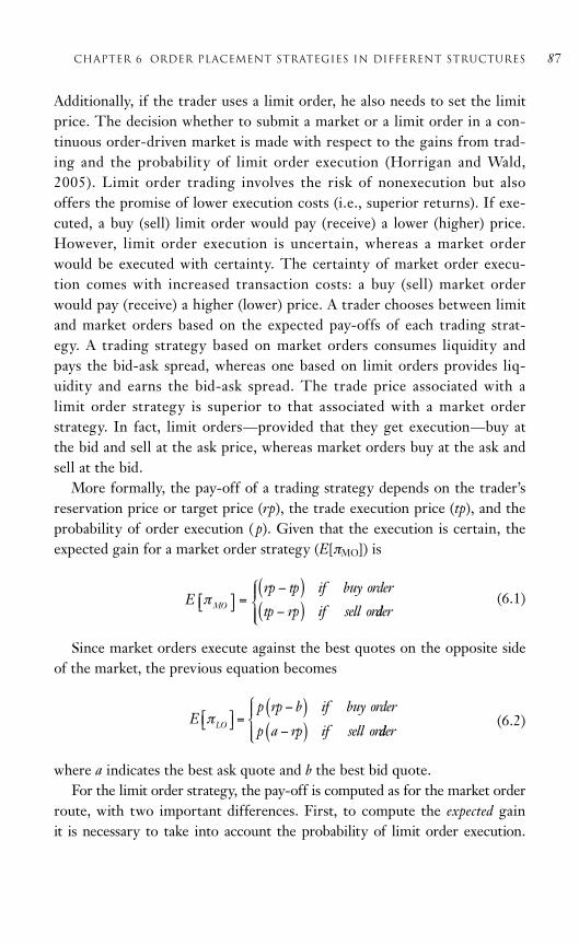
Additionally, if the trader uses a limit order, he also needs to set the limitprice. The decision whether to submit a market or a limit order in a con-tinuous order-driven market is made with respect to the gains from trad-ing and the probability of limit order execution (Horrigan and Wald,2005). Limit order trading involves the risk of nonexecution but alsooffers the promise of lower execution costs (i.e., superior returns). If exe-cuted, a buy (sell) limit order would pay (receive) a lower (higher) price.However, limit order execution is uncertain, whereas a market orderwould be executed with certainty. The certainty of market order execu-tion comes with increased transaction costs: a buy (sell) market orderwould pay (receive) a higher (lower) price. A trader chooses between limitand market orders based on the expected pay-offs of each trading strat-egy. A trading strategy based on market orders consumes liquidity andpays the bid-ask spread, whereas one based on limit orders provides liq-uidity and earns the bid-ask spread. The trade price associated with alimit order strategy is superior to that associated with a market orderstrategy. In fact, limit orders—provided that they get execution—buy atthe bid and sell at the ask price, whereas market orders buy at the ask andsell at the bid.
More formally, the pay-off of a trading strategy depends on the trader’sreservation price or target price (rp), the trade execution price (tp), and theprobability of order execution ( p). Given that the execution is certain, theexpected gain for a market order strategy (E[πMO]) is
(6.1)
Since market orders execute against the best quotes on the opposite sideof the market, the previous equation becomes
(6.2)
where a indicates the best ask quote and b the best bid quote.For the limit order strategy, the pay-off is computed as for the market order
route, with two important differences. First, to compute the expected gain it is necessary to take into account the probability of limit order execution.
chapter 6 Order Placement Strategies in Different structures 87
Erp tp if buy order
tp rp if sell orMOπ⎡⎣ ⎤⎦ =−( )−( ) dder
⎧⎨⎪
⎩⎪
Ep rp b if buy order
p a rp if sell orLOπ⎡⎣ ⎤⎦ =−( )
−( ) dder
⎧⎨⎪
⎩⎪

Second, the execution price associated with a limit order strategy is strictlybetter than that associated with the market order strategy. The expected gainfor a limit order strategy (E[πLO]) is
(6.3)
The break-even conditions for buy and sell orders between market orderand limit order strategies can be stated as follows
(6.4)
Based on Equation 6.4—which in turn is based on Equation 6.1, Equa-tion 6.2, and Equation 6.3—it is possible to derive a break-even probabilityas the probability value that equates the expected gains associated with limitorder placement and market order submission. The break-even probability( pBE) for a buy order is
(6.5)
where s indicates the bid-ask spread.Equation 6.5 can be used to decide the best trading strategy by compar-
ing the break-even probability of limit order execution with the actualprobability of limit order execution. If the break-even probability is higherthan the actual, it is preferable to submit a market order, otherwise a limitorder would be preferable. Equation 6.5 also implies that the higher thereservation price is, the higher the break-even probability, and the moreappropriate is to place a market order. In fact, as the reservation priceincreases, the differential gain between limit order and market order van-ishes. Additionally, Equation 6.5 implies that the higher is the bid-askspread, the lower is the break-even probability, and the less suitable is touse a market order since it would imply a largely inferior execution pricewith respect to a limit order strategy.
The probability of limit order execution strongly affects the expectedgain from limit order trading and, consequently, the choice between limitand market orders. Five factors affect the probability of limit order execu-tion (Hollifield, Miller, and Sandas, 2004): the aggressiveness of the limit
88 Part i EXECUTION A ND MOMENTUM TR ADING
Ep rp b if buy order
p a rp if sell orLOπ⎡⎣ ⎤⎦ =−( )
−( ) dder
⎧⎨⎪
⎩⎪
p rp arp b
rp b srp b
srp bBE =
−−
=− −
−= −
−1
( ) ( )( ) ( )rp a p rp b if buy orderb rp p a rp if sel
− = −
− = − ll order

price, the depth of the book, the rate of market orders, the duration of theorder, and the volatility of stock returns. First, for buy orders, the higherthe limit price, the higher the probability of execution; for sell orders, thelower the limit price, the higher the probability of execution. Second, thelarger the size of depth on the buy (sell) side, the lower the probability ofexecution for a buy (sell) limit order. Third, the larger the arrival rate of amarket order on the opposite side of the market, the higher the probabilityof execution for a limit order. Fourth, the longer the duration of the limitorder, the higher the probability of execution. Fifth, the larger the pricevolatility, the higher the probability of execution for a limit order, whichdoes not imply that order execution will be profitable; it simply implies thathigher volatility entails higher probability of execution. Execution is prof-itable for a limit order trader if the volatility that triggered the limit orderexecution is temporary. Execution is unprofitable for a limit order trader ifthe volatility that triggered the limit order execution is permanent.
Three implications arise from the previous discussion. First, high volatil-ity days or high volatility stocks make convenient to use limit orders. Traders might even place limit orders on both sides of the market, acting asmarket makers, to benefit from accentuated intraday volatility (Petrella,2006). Second, relatively patient traders place limit orders. This strategy isusually called passive trading strategy (PTS). Large investors may preferPTS because this strategy does not cause market prices to change (due tomarket impact) as the orders are naturally absorbed by the market. Third,relatively eager traders place market orders. In a dynamic setting, a tradermight define an order placement strategy where he first uses limit orders (as a patient trader) and then switches to market orders (that is, he becomesimpatient) to trade the quantity associated with unexecuted limit orders.
TRADING IN A CALL AUCTION
In a call auction, multiple orders are batched together periodically for asimultaneous execution (Economides and Schwartz, 1995). At the time ofthe call, a market clearing price that maximizes the tradable quantity isdetermined and applied to execute all matchable orders. In a continuousorder-driven market, trades are made whenever matchable buy and sellorders happen to cross. By contrast, in a call auction, trades are made atspecific points in time when the market clearings are held (e.g., at the open,at the close, and/or at specific times during the trading day).
chapter 6 Order Placement Strategies in Different structures 89

Call auctions differ from continuous order-driven markets along threedimensions. First, in terms of immediacy, waiting time (execution speed) islower (higher) in continuous markets. Second, in terms of price discovery,prices in call markets are better than in continuous markets. Prices arehighly volatile in continuous markets because of news (efficient volatility)and order imbalance (ineff icient volatilit y). Traders get their orders executed depending on the current market conditions at the time of thesubmission. By contrast, in a call auction, the terms of the trade depends onthe cumulative market conditions at the end of the preopening phase. Thisimplies that a transitory order imbalance might be easily wiped out in a callauction by orders arriving from the opposite side of the market and thusreducing inefficient volatility (i.e., temporary price swings). Third, in termsof trading volume, volume is higher in continuous markets. Some tradersthat do not get execution in a call market, may execute their trades in acontinuous market (with zero surplus) if, on the opposite side of the market,there are impatient traders demanding liquidity. In short, continuous markets sacrifice surplus (i.e., expected profits) for immediacy, whereas callauctions sacrifice immediacy for a better price discovery process.
Trading in a call auction is only apparently equivalent to trading in acontinuous market. Orders entered in a call auction are executed accordingto the standard price priority rule followed by the time priority rule, just asin continuous order-driven markets. However, limit and market orders arehandled differently in call and continuous trading and, consequently, theyshould be submitted differently.
The operation of a call auction has two main implications for the designof trading strategies. First, executed orders receive price improvement in acall auction (Schwartz, Francioni, and Weber, 2006). In fact, there is nobid-ask spread in a call auction because all executed orders clear at the sameprice. Almost all executed orders receive price improvement (or positivesurplus or positive expected profits). Precisely, buy orders priced above thesingle clearing price and sell orders priced below it receive price improve-ment. Only orders priced exactly at the clearing price do not receive priceimprovement. Second, traders are more aggressive in a call auction. In acontinuous market, limit orders provide immediacy and set the prices,whereas market orders demand immediacy and accept limit orders prices.The limit price affects the probability of execution and sets the price. In acall market, all participants wait until the market will be “called” and allorders executed simultaneously. Both limit order and market order traders
90 Part i EXECUTION A ND MOMENTUM TR ADING

supply liquidity to each other. The market clearing price will be determinedby the equilibrium between the overall demand and the overall supply. Thelimit price affects the probability of execution, but it does not set the price(although it does affect the market clearing price). Precisely, the impact ofan order on the clearing price depends on the size of the order with respectto the rest of the market. If such order is small in size, it will not affect theclearing price. The previous discussion implies that, in a call auction, atrader has a strong incentive to place an aggressively priced order since hewill not pay the aggressive price for the stock, because the clearing pricewill be set by the overall demand and supply, but he will benefit from such aprice that will be used to set the orders that will be executed in the call auc-tion according to the price priority rule.
CONCLUSION
In this chapter, we study how the optimal trader’s strategy differs acrossmarket structures. The choice between limit orders and market orders is animportant component of the order placement strategy. Limit orders supplyliquidity to the markets because they provide other traders an opportunityto trade at specified conditions (i.e., the limit price). By placing a limit order,a trader enters in a position that is comparable to a short option position. A buy limit order, e.g., is equal to a short position in an American-style putoption as the trader extends to anyone in the market the right to sell a certain number of shares (equal to the size of the order) at a certain price(equal to the limit price of the order). By contrast, market orders demandliquidity because they consume the liquidity offered by limit orders. Thechoice between limit orders and market orders depends on the gains fromtrading and the probability of execution.
Our analysis highlights several implications for trading strategies in continuous order-driven markets and call auctions. In a continuous order-driven market, the gains from trading by limit orders depend on the size ofthe bid-ask spread. The larger is the bid-ask spread, the larger is the bene-fit for a limit order trader, if the limit order executes. In a call auction,there is no bid-ask spread and almost all executed orders receive priceimprovement.
As for the probability of execution, in a continuous order-driven mar-ket, the probability of limit order execution depends on the limit price andmarket conditions. A more aggressive price increases the probability of
chapter 6 Order Placement Strategies in Different structures 91

execution, but it lowers the benefit of limit order trading. As for the mar-ket conditions, if prices are moving to a new level (permanent volatility),the trader should use a market order and settle for the current price;whereas, if prices are fluctuating around and will revert back to a previouslevel (transitory volatility), the trader should be patient and use a limitorder. In a call auction, limit prices determine the precedence and (may)affect the market clearing price, but they are not execution prices. Conse-quently, limit order traders are more aggressive in call auctions since theywill not pay the aggressive price, but they will benefit from it in terms ofhigher probability of execution.
REFERENCES
Anolli, M. and Petrella, G. (2007) Internalization in European Equity MarketsFollowing the Adoption of the EU MiFID Directive. Journal of Trading,2(2): 77–88.
Economides, N. and Schwartz, R.A. (1995) Electronic Call Market Trading.Journal of Portfolio Management, 21(3): 10–18.
Foucault, T. (1999) Order Flow Composition and Trading Costs in aDynamic Limit Order Market. Journal of Financial Markets, 2(2):99–134.
Handa, P. and Schwartz, R.A. (1996) Limit Order Trading. Journal ofFinance, 51(5): 1835–1861.
Handa, P., Schwartz, R.A., and Tiwari, A. (1998) The Ecology of anOrder-Driven Market. Journal of Por t folio Management, 24(2):47–55.
Harris, L.E. (1998) Optimal Dynamic Order Submission Strategies inSome Stylized Trading Problems. Financial Markets, Institutions &Instruments, 7(2): 1–76.
Harris, L.E. (2003) Trading and Exchanges. Oxford University Press: New York.
Hollifield, B., Miller, R.A., and Sandas, P. (2004) Empirical Analysis ofLimit Order Markets. Review of Economic Studies, 71(4): 1027–1063.
Horrigan, H.T. and Wald, J.K. (2005) Optimal Limit Order Choice. Journalof Business, 78(2): 597–619.
92 Part i EXECUTION A ND MOMENTUM TR ADING

Petrella, G. (2006) Option Bid-Ask Spread and Scalping Risk: Evidencefrom a Covered Warrants Market. Journal of Futures Markets, 26(9):843–867.
Schwartz, R.A., Francioni, R., and Weber, B. (2006) The Equity TraderCourse. Hoboken, NJ: John Wiley & Sons.
chapter 6 Order Placement Strategies in Different structures 93

This page intentionally left blank

P A R T I I
TECHNICALTR ADING

This page intentionally left blank
97
7C H A P T E R
Profitability of TechnicalTrading Rules in an EmergingMarket
Dimitris Kenourgios and Spyros Papathanasiou
ABSTRACT
This chapter investigates the profitability of technical trading rules in theAthens Stock Exchange (ASE), utilizing the FTSE/ASE 20 index duringthe period 1995 to 2008. We focus on a less developed and efficient stockmarket, given the existing scarcity of research in such markets. The techni-cal rules that will be explored are simple moving averages. We comparetechnical trading strategies in the spirit of Brock, Lakonishok, and LeBaron(1992), employing traditional t test and bootstrap methodology under thegeneralized autoregressive conditional heteroskedasticity model. Theresults provide strong evidence on the profitability of the technical tradingrules against the “buy and hold” strategy and contradict the efficient markethypothesis.
INTRODUCTION
This chapter explores the profitability of simple technical rules in theAthens Exchange Market (ASE) and particularly for the FTSE/ASE 20 index. The FTSE/ASE 20 is the most important index of the ASE andrepresents the 20 companies with the largest capitalization. The technicaltrading rules that we use to evaluate the profitability of technical analysisagainst the buy and hold strategy (benchmark) are variations of the simplemoving average rule.
Technical analysis forecasts the future direction of prices through thestudy of past market data, primarily price, and volume. In its simplest form,technical analysis considers only the actual price and volume behavior of themarket. Moving averages help traders to track the trends of financial assetsby smoothing out the day-to-day price fluctuations, or noise. Although themajority of the professional traders and investors use technical analysis,most academics, until recently, had not recognized the validity of thesemethods.
Technical anomalies are observed in most developed and developing mar-kets, leading traders and investors to earn significant abnormal returns.This chapter investigates these anomalies which appear to be in contrastwith the efficient market hypothesis (EMH). A financial market can be con-sidered as efficient if prices fully reflect all available information and noprofit opportunities are left unexploited (Fama, 1965, 1970; Fama andFrench, 1988). The agents form their expectations rationally and rapidlyarbitrage away any deviations of the expected returns consistent with supernormal profits. Therefore, it is the EMH and the random walk theoryversus practice.
The methodology that is employed for the analysis of the data is the traditional t test, which has been used in many prior studies for the investi-gation of technical anomalies (e.g., Brown and Jennings, 1989; Neftci,1991; Gençay, 1998). In addition, we compare the t test results with thoseobtained by bootstrap methodology. Bootstrapping, introduced by Efron(1979), is a method for estimating properties of an estimator (such as itsvariance) by measuring those properties when sampling from an approxi-mating distribution. One standard choice for an approximating distributionis the empirical distribution of the observed data. In the case where a set of observations can be assumed to be from an independent and identically
98 Part i I TECHNICAL TR ADING

distributed population, this can be implemented by constructing a numberof resamples of the observed dataset (and of equal size to the observeddataset), each of which is obtained by random sampling with replacementfrom the original dataset. Following bootstrap methodology, we use thereturns generated from the pseudo ASE series and we apply the tradingrules to the series. Therefore, comparisons are then made between returnsfrom these simulated series and the original ASE series.
Among the international studies examining the technical anomalies,Brock, Lakonishok, and LeBaron (1992), hereafter BLL (1992), investi-gate two popular trading rules (moving average and trading range breakrule), utilizing the Dow Jones Index from 1897 to 1986. Overall, theirresults provide strong support for the technical strategies. Kwon andKish (2002) provide an empirical analysis on technical trading rules (thesimple moving average, the momentum, and trading volume), utilizingthe NYSE value-weighted index over the period 1962 to 1996. Theirresults indicate that the technical trading rules can capture profit oppor-tunities over a buy-hold strategy. In addition, Wong, Manzur, and Chew(2003) examine the role of technical analysis in signaling the timing ofstock market entry and exit for the Singapore stock market. They testthe performance of moving average and the relative strength index andfind that the applications of technical indicators provide substantial prof-its. Further, Atmeh and Dobbs (2006) investigate the performance ofvarious moving average rules in the Jordanian stock market. Their resultsshow that technical trading rules can help to predict market movements,and there is some evidence that (short) rules may be profitable afterallowing for transactions costs.
The research on technical anomalies for the Athens Stock Exchange isstill very limited. Vasiliou, Eriotis, and Papathanasiou (2008a) examine theperformance of various types of technical trading rules in the Athens StockExchange, during the period 1995 to 2005. In particular, this study exam-ines the predictability of daily returns using various moving averages rulesfor the Athens General Index. Their results provide strong support for theexamined technical strategies. Vasiliou, Eriotis, and Papathanasiou (2008b)apply technical analysis methodology into the behavior theory for the largecapitalization firms of the ASE from 1995 to 2005. Using standard andmore complicated tests, they provide evidence of a strong increase in trad-ing rules performance over time.
chapter 7 TECHNICAL TR ADING RULES in Emerging Markets 99
This study is significant for three reasons. First, it focuses on a lessdeveloped and efficient stock market, given the existing paucity of researchin such markets. Second, in contrast to prior relevant studies, it examinesthe profitability of technical trading rules after considering transactioncosts imposed to the participants in the ASE. Finally, traders would benefitfrom this research, as they will find that these technical rules work in theASE and are definitely profitable, since they have been tested with statisticaland more advanced econometric methods.
The structure of this chapter is organized as follows: The second sectionof this chapter analyzes methodological issues. The third section presentsthe data and the empirical findings of the research. The final section con-tains the concluding remarks.
METHODOLOGY
In order to evaluate the performance of simple moving averages, we com-pare the returns given by the buy signals of the moving average with thereturns of the buy and hold strategy. In addition, we compare the returnsgiven by the buy signals of the moving average minus the returns of the sellsignals of the moving average with the returns of the buy and hold position.We then calculate the returns after transaction costs. All transactionsassume commission as entry and exit fees (0.2 percent of the investing capital).
First, we examine whether moving averages produce better results thanthe buy and hold strategy using the standard t test. Moving averages give buysignal when the short-term moving average crossover the long-term one. Onthe other side, we have a sell signal when the long-term moving averagecrossover the short-term one. Historically, moving average crossovers tend tolag the current market action.
We use t test in order to assess if the means of two data groups are statistically different from each other in order to compare these means. Wecalculate the t statistic using the following formulas:
(7.1)
100 Part i I TECHNICAL TR ADING
µ µ
σ σ
buys sells buy hold
observ buys s
( ) &
. (
(
−
+2 2
Ν Ν eells )
)

(7.2)
where σ2 is the square root of the standard deviation of the returns, µ is themean return for the buys, sells, and buy and hold position, and N is thenumber of signals for the buys, sells, and observations.
Using t tests, we compare the mean returns of the unconditional buymethodology with the returns of the buy signals given by the moving averagesand the returns of the unconditional buy methodology with the returns of thebuy signals minus the returns of the sell signals given by the moving averages.The results provided by the t test will help to either accept the null hypothesis(there is no actual difference between mean returns) or reject it (there is anactual difference between the mean returns).
It is well known that the results obtained by t test assume independent,stationary, and asymptotically normal distributions. However, it is quitecommon that financial time series exhibit non-normality based on excessiveskewness, kurtosis, and heteroskedasticity. Following BLL (1992), we over-come these statistical problems adopting the bootstrap technique. Bootstrapis a computer-based resampling procedure introduced by Efron (1979),which has been discussed in the statistics and econometrics literature overthe past 20 years (e.g., Efron, 1987; Freedman and Peters, 1984a, 1984b;Veall, 1992). This method requires no analytical calculations and the proce-dure uses only the original data for resampling to access the unobservablesampling distribution and to provide a measure of sampling variability, bias,and confidence intervals. Efron and Tibshirani (1986) propose that the useof the bootstrap enlarges the type of statistical problem that can be analyzed, reduces the assumptions required to validate the analyses, andeliminates the tedious theoretical calculations associated with the assessmentof accuracy.
The idea behind the bootstrap is to use resampling to estimate anempirical distribution for the statistic. The procedure of the bootstrapmethodology is the following: First, we create Z bootstrap samples, eachconsisting of N observations by sampling with replacement from the origi-nal return series. Second, we calculate the corresponding price series foreach bootstrap sample, apply the moving average rule to each of the Z artificial price-series and calculate the performance statistic of interest
chapter 7 TECHNICAL TR ADING RULES in Emerging Markets 101
µ µ
σ σ
buys sells
buys sells
−
+( )2 2
Ν Ν

for each of the pseudo price series. Finally, we determine the p value bycalculating the number of times the statistic from the pseudo series exceedthe statistic from the original price series. In order to use the bootstrapmethod, a data generating process for market prices or returns must bespecified a priori. The bootstrap method can be used to generate many dif-ferent return series by sampling with replacement from the original returnseries. The bootstrap samples created are pseudo return-series that retainall the distributional properties of the original series, but are purged of anyserial dependence.
Financial time series usually exhibit a characteristic known as volatilityclustering, in which large changes tend to follow large changes, and smallchanges tend to follow small changes. In either case, the changes from oneperiod to the next are typically of unpredictable sign. Volatility clustering,or persistence, suggests a time-series model in which successive distur-bances, although uncorrelated, are nonetheless serially dependent.
To account for the phenomenon of volatility clustering, which is verycommon in financial time series, the model we use is the generalizedautoregressive conditional heteroskedasticity, or GARCH (1,1), model,proposed initially by Engle (1982) and further developed by Bollerslev(1986). The specification of the GARCH (1,1) model is the following:
(7.3)
where r is the return of the stock index, σ2 is the variance, the residuals εt
are conditionally normally distributed with zero mean and conditional variance (σ2), and the standardized residuals are independent and identicallydistributed N(0,1). The variance equation is a function of three terms: themean ω, news about volatility from the previous period, measured as the lagof the squared residual from the mean ε2
t1 equation (α is the ARCH term),and last period’s forecast variance σ 2
t1 (β is the GARCH term). The sum ofARCH and GARCH coefficients (α β) indicates the degree of persistencein volatility. Values of (α β ) close to unity imply that the persistence involatility is high.
In order to use bootstrap under GARCH (1,1), we first estimate theGARCH (1,1) by using maximum likelihood and apply the bootstrapmethod on the standardized residuals. Then produce GARCH series byusing the estimated parameters and the crumbled residuals. In this chapter,
102 Part i I TECHNICAL TR ADING
r rt t t
t t t
= + +
= + +−
− −
γ δ ε
σ ω αε βσ1
21
21
2

each of the simulations is based on 500 replications of the null model,which should provide a good approximation of the return distributionunder the null model.
To test the significance of the trading rule excess returns, the followinghypothesis can be stated:
(7.4)
Under the null hypothesis (H0), the trading rule excess return (XR) cal-culated from the original series is less than or equal to the average tradingrule return for the pseudo data samples (X
–R*). The p values from the boot-
strap procedure are then used to determine whether the trading rule excessreturns are significantly greater than the average trading rule return giventhat the true data-generating process is GARCH (1,1).
DATA AND EMPIRICAL RESULTS
In this study, we use daily closing prices of the FTSE/ASE 20 index from1/1/1995 to 31/12/2008. The database used is composed of 3,249 observa-tions. The FTSE/ASE 20 index is one of the most famous indexes of theASE and includes the 20 companies with the largest capitalization. Therequirements for the firms to participate in this index are the capitalization,marketability, and the free-float. The index of the Athens Stock Exchangewas designed with the cooperation of the London Stock Exchange andFTSE International Limited.
We evaluate the performance of the following moving average rulesagainst the buy and hold strategy: (1,9), (1,15), (1,30), (1,60), (1,90),(1,120), and (1,150). The first number in each pair indicates the days in theshort period and the second number shows the days in the long period.
Standard Statistical Results
Table 7.1 reports some summary descriptive statistics for the daily returnsof the FTSE/ASE 20 index. We calculate the returns as log differences ofthe FTSE/ASE 20 level. We observe that the returns exhibit excessive(lepto) kurtosis and non-normality.
chapter 7 TECHNICAL TR ADING RULES in Emerging Markets 103
H XR XR
H XR XR
0
1
:
:
*
*_
≤−

104 Part i I TECHNICAL TR ADING
Table 7.1 Descriptive Statistics
Num 3,249
Maximum 0.0877
Minimum 0.0973
Mean 0.000531183
Median 0.000174311
Range 0.1922
Standard Deviation 0.0178
Skewness 0.0759
Kurtosis 6.7123
JB statistic 0.000151223
JB p value 0.0000
Buy-hold mean return 0.00020439
(after fees)
The JB statistic is Jarque and Bera’s (1987) test for normality, being distributedas x2 with 2 degrees of freedom under the null of normal distribution.
Table 7.2 presents the results using simple moving average trading strate-gies. The rules differ by the length of the short and long period. For exam-ple, (1,60) indicates that the short period is one day and the long period is 60days. We report the number of buy “N(Buy)” and sell “N(Sell)” signals gen-erated during the period in columns 3 and 4. The mean buy and sell dailyreturns are reported separately in columns 5 and 6, while column 7 lists thedifferences between the mean buy and sell daily returns (“Buy/Sell”). Thesetests are computed using the BLL (1992) method.
We observe in column 7 that the buy/sell differences are significantlypositive for all rules. This leads to the rejection of the null hypothesis(equality with zero). The mean buy/sell returns are all positive with anaverage daily return of 0.0987 percent. This is 24.675 percent on a yearbasis (250 trading days 0.0987 percent).
The mean buy returns are all positive with an average daily return of 0.0669 percent. This is 16.725 percent on a year basis (250 trading days 0.0669 percent). The t statistics reject the null hypothesis since the meanreturn of the buy and hold position is 0.020439 percent (see Table 7.1). Sixof the seven tests reject the null hypothesis that the returns equal theunconditional returns at the 5 percent significance level using a two-tailedtest. About the sells, the daily average return is 0.00318 percent. This is7.95 percent on a year basis. All the tests also reject the null hypothesis atthe 5 percent significance level.

If technical analysis does not have any power to forecast price move-ments, then we should observe that returns on days when the rules emitbuy signals do not differ appreciably from returns on days when the rulesemit sell signals. In this chapter, we provide evidence that the technicalstrategies used win the buy and hold strategy (FTSE /ASE 20). Overall,the buy and hold strategy (see Table 7.1) gives 5.10975 percent annualreturn (0.020439 250 days), while the strategy of simple moving aver-ages 24.675 percent.
Bootstrap Results
Following BLL (1992) methodology, we create 500 bootstrap samples,each consisting of 3,249 observations by resampling with replacement the
chapter 7 TECHNICAL TR ADING RULES in Emerging Markets 105
Table 7.2 Standard Results for the Simple Moving Average Rules
N(Buy) N(Sell) Buy Sell(Long (Short (Long (Short
Period Test Strategy) Strategy) Strategy) Strategy) Buy/Sell(1) (2) (3) (4) (5) (6) (7)
1/1/1995 to12/31/2008 (1,9) 336 336 0.000938 -0.000275 0.001213
(2.1504) (-4.3182) (3.5765)
(1,15) 238 238 0.000911 -0.000240 0.001151
(2.0271) (-4.1216) (3.3562)
(1,30) 140 139 0.000856 -0.001084 0.00194
(2.5425) (-3.04105) (5.31961)
(1,60) 97 97 0.000762 -0.000648 0.00141
(2.33062) (-3.00431) (5.20577)
(1,90) 67 68 0.000625 -0.000383 0.001008
(2.01446) (-2.48048) (3.88020)
(1,120) 58 59 0.000577 -0.00279 0.000856
(1.98212) (-2.38126) (3.18968)
(1,150) 44 45 0.000571 -0.000039 0.000010
(1.95453) (-2.11723) (3.21245)
Average 0.000669 0.000318 0.000987
N(Buy) and N(Sell) are the number of buy and sells signals generated by the rule.
In columns 5, 6, and 7, the number in parentheses are standard t statistics, testing the difference between the meanbuy return and the unconditional mean return, the mean sell return and the unconditional mean return, and buy/selland zero, respectively.
The last row reports averages across all seven rules.
The upper (lower) critical values of the t test values are 1.96 at 5% level.

standardized residuals of the GARCH (1,1) model. Then, we generateGARCH price-series by using the estimated parameters and the crumbledresiduals. After that, we apply the moving averages to each of the 500pseudo price-series. Then, we determine the p value by calculating thenumber of times the statistic from the artificial series exceeds the statisticfrom the original price series (FTSE/ASE 20 index).
Table 7.3 presents the estimates of the GARCH (1,1) model. Based onthe Akaike Information Criterion, the Schwarz Criterion, and Dickey-Fuller and Phillips-Perron unit root tests, we find that the GARCH (1,1)model is well specified.1 Values of α β close to unity imply that the per-sistence in volatility is high. In our case, the sum of the ARCH andGARCH coefficients (α β) is very close to one indicating that volatilityshocks are very persistent.
Table 7.4 displays the results of GARCH (1,1) simulations using simplemoving average trading strategies via bootstrapping. We present results forthe seven moving average rules that we examine. All the numbers presentedin columns 4, 5, and 6 are the fractions of the simulated result which arelarger than the results for the original FTSE/ASE 20 index. We report themean buy and sell returns separately in columns 4 and 5. The results pre-sented in columns 4, 5, and 6 are p values. The p values from the bootstrapprocedure are then used to determine whether the trading rule excessreturns (simple moving averages) are significantly greater than the averagetrading rule return given from original series. The numbers in parenthesesin columns 4, 5, and 6 show how many series from 500 replications aregreater than the original returns.
106 Part i I TECHNICAL TR ADING
Table 7.3 Estimates of GARCH (1,1) Model
γ δ ω α β
0.00040308 0.18353 0.000434 0.12836 0.86487
(1.7439) (9.2178) (5.5613) (14.4956) (108.6476)
We estimate the following GARCH (1,1) model:
rt γ δrt1 εt
σ2t ω αε2
t1 βσ 2t1
where r is the return of the stock index, σ 2 is the variance, the residuals εt are conditionally normallydistributed with zero mean and conditional variance (σ 2), the standardized residuals are independent andidentically distributed N(0,1), α is the ARCH term, and β is the GARCH term.
Estimated on daily returns series of the FTSE/ASE 20 index for the period 1/1/1995 to 12/31/2008.
Numbers in parentheses are t ratios.
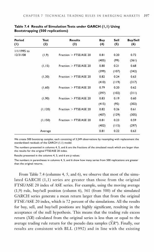
From Table 7.4 (columns 4, 5, and 6), we observe that most of the simu-lated GARCH (1,1) series are greater than those from the originalFTSE/ASE 20 index of ASE series. For example, using the moving average(1,9) rule, buy/sell position (column 6), 361 (from 500) of the simulatedGARCH series generate a mean return larger than that from the originalFTSE /ASE 20 index, which is 72 percent of the simulations. All the resultsfor buy, sell, and buy/sell positions are highly significant, resulting in theacceptance of the null hypothesis. This means that the trading rule excessreturn (XR) calculated from the original series is less than or equal to theaverage trading rule return for the pseudo data samples (X
–R*). Finally, our
results are consistent with BLL (1992) and in line with the existing
chapter 7 TECHNICAL TR ADING RULES in Emerging Markets 107
Table 7.4 Results of Simulation Tests under GARCH (1,1) UsingBootstrapping (500 replications)
Period Test Results Buy Sell Buy/Sell(1) (2) (3) (4) (5) (6)
1/1/1995 to12/31/08 (1,9) Fraction FTSE/ASE 20 0.81 0.20 0.72
(405) (99) (361)
(1,15) Fraction FTSE/ASE 20 0.80 0.21 0.68
(399) (107) (342)
(1,30) Fraction FTSE/ASE 20 0.82 0.24 0.63
(410) (119) (317)
(1,60) Fraction FTSE/ASE 20 0.79 0.20 0.62
(397) (102) (311)
(1,90) Fraction FTSE/ASE 20 0.83 0.19 0.60
(415) (95) (302)
(1,120) Fraction FTSE/ASE 20 0.82 0.26 0.61
(407) (129) (305)
(1,150) Fraction FTSE/ASE 20 0.81 0.23 0.59
(402) (115) (297)
Average 0.81 0.22 0.63
We create 500 bootstrap samples, each consisting of 3,249 observations by resampling with replacement thestandardized residuals of the GARCH (1,1) model.
The numbers presented in columns 4, 5, and 6 are the fractions of the simulated result which are larger thanthe results for the original FTSE/ASE 20 index.
Results presented in the columns 4, 5, and 6 are p values.
The numbers in parentheses in columns 4, 5, and 6 show how many series from 500 replications are greaterthan the original returns.

evidence on the profitability of technical trading strategies in emerging andless developed stock markets.
CONCLUSION
This chapter investigates the profitability of technical trading rules in anemerging market such as the Athens Stock Exchange. Particularly, we usevariations of simple moving averages for the FTSE/ASE 20 index, usingdaily data for the period 1995 to 2008. Following the BLL (1992)methodology, we evaluate the performance of seven moving averagesrules (1,9), (1,15), (1,30), (1,60), (1,90), (1,120), and (1,150) against the buy and hold strategy, using both standard tests and bootstrapmethodology.
Using t tests, we compare the mean returns of the unconditional buymethodology with the returns of the buy signals given by the moving aver-ages and the returns of the unconditional buy methodology with thereturns of the buy signals minus the returns of the sell signals given by themoving averages. In this setup, we test the null hypothesis (there is noactual difference between mean returns) against the alternative (there is anactual difference between the mean returns). Using bootstrap methodol-ogy, we compare the returns conditional on buy (or sell) signals from theactual FTSE/ASE 20 data with the returns from simulated comparisonseries generated by a model from the null hypothesis class being tested.The null model tested is the GARCH (1,1).
About the simple moving averages trading strategies, we find that allthe buy/sell differences are positive. Also, all the t tests for the differ-ences are highly significant rejecting the null hypothesis (equality withzero). In addition, the mean buy/sell returns are all positive with a dailyreturn of 0.0987 percent in average (24.675 percent annual return).Overall, the results indicate that making trading decisions based on mov-ing average rules lead to significantly higher returns than the buy andhold strategy, even after transaction costs. In addition, the results showthat technical rules produce useful signals and can help to predict marketmovements. More specific, the profitability of technical strategies such as moving averages on large capitalization stocks is better than the profitability we get by simply following the market (buy and hold). Inparticular, the buy and hold strategy gives 5.10975 percent annual
108 Part i I TECHNICAL TR ADING

return, while simple moving averages 24.675 percent (buy/sell) on anannual basis. Using bootstrapping, the results are quite similar. Most ofthe simulated GARCH (1,1) series are greater than those from the origi-nal FTSE/ASE 20 index of ASE series. Our results are in line with theexisting literature on the performance of technical trading rules inemerging and less developed stock markets.
Our findings contradict to the efficient market hypothesis as traders andinvestors can gain abnormal returns using moving average trading strate-gies. Furthermore, our results (after transactions costs) are consistent withthe simple technical rules having predictive power. Finally, the profitabilityof the applied technical strategies in this chapter is verified by using econo-metrical and statistical methods. Our research indicates that the benefits oftechnical trading strategies, such as the prediction of price movements andthe identification of trends and patterns, can be exploited by traders to earnsignificant returns on the ASE.
REFERENCES
Atmeh, M. and Dobbs, I.M. (2006) Technical Analysis and the StochasticProperties of the Jordanian Stock Market Index Return. Studies in Economics and Finance, 23(2): 119–140.
Bollerslev, T. (1986) A Generalized Autoregressive Condit ional Heteroscedasticity. Journal of Econometrics, 31(3): 307–327.
Brock, W., Lakonishok, J., and LeBaron, B. (1992) Simple Technical Trad-ing Rules and the Stochastic Properties of Stock Returns. Journal ofFinance, 47(5): 1731–1764.
Brown, D.P. and Jennings, R.H. (1989) On Technical Analysis. Review ofFinancial Studies, 2(4): 527–551.
Efron, B. (1979) Bootstrapping Methods: Another Look at the Jacknife.Annals of Statistics, 7(1): 1–26.
Efron, B. (1987) Better Bootstrap Confidence Intervals (with discussion).Journal of the American Statistical Association, 82: 171–200.
Efron, B. and Tibshirani, R.J. (1986) Bootstrap Methods for StandardErrors, Confidence Intervals and other Measures of Statistical Accuracy.Statistical Science, 1(1): 54–77.
chapter 7 TECHNICAL TR ADING RULES in Emerging Markets 109

Engle, R. (1982) Autoregressive Conditional Heteroskedasticity with Estimates of the Variance of United Kingdom Inflation. Econometrica,50(4): 987–1008.
Fama, E. (1965) The Behaviour of Stock Market Prices. Journal of Business,38(1): 34–105.
Fama, E. (1970) Efficient Capital Markets: A Review of Theory and EmpiricalWork. Journal of Finance, 25(2), 383–417.
Fama, E. and French, K. (1988) Permanent and Temporary Components ofStock Prices. Journal of Political Economy, 96(2): 246–274.
Freedman, D. and Peters, S.C. (1984a) Bootstrapping a Regression Equation:Some Empirical Results. Journal of the American Statistical Association,79(385): 97–106.
Freedman, D. and Peters, S.C. (1984b) Bootstrapping an Econometric Model:Some Empirical Results. Journal of Business and Economic Statistics, 2(2):150–158.
Gençay, R. (1998) The Predictability of Securities Returns with SimpleTechnical Rules. Journal of Empirical Finance, 5(4): 347–359.
Jarque, C. M., and Bera, A. K. (1987) A Test for Normality of Observationsand Regression Residuals. International Statistical Review. 55(2):163–172.
Kwon, K.Y. and Kish, R.J. (2002) Technical Trading Strategies and ReturnPredictability: NYSE. Applied Financial Economics, 12(9): 639–653.
Neftci, S. (1991) Naive Trading Rules in Financial Markets and Weiner-Kologorov Prediction Theory: A Study of Technical Analysis. Journalof Business, 64(4): 549–571.
Vasiliou, D., Eriotis N., and Papathanasiou, S. (2008a) Technical TradingProfitability in Greek Stock Market. The Empirical Economics Letters,7(7): 749–756.
Vasiliou, D., Eriotis N., and Papathanasiou, S. (2008b) Incorporating Tech-nical Analysis into Behavioral Finance: A Field Experiment in theLarge Capitalization Firms of the Athens Stock Exchange. InternationalResearch Journal of Finance and Economics, 9(14): 100–112.
Veall, M.R. (1992) Bootstrapping the Process of Model Selection: An Econometric Example. Journal of Applied Econometrics, 7(1): 93–99.
110 Part i I TECHNICAL TR ADING

Wong, W.K., Manzur M., and Chew, B.K. (2003) How Rewarding is Technical Analysis? Evidence from Singapore Stock Market. AppliedFinancial Economics, 13(7): 543–551.
NOTES
1. Results, not presented here, are available upon request.
chapter 7 TECHNICAL TR ADING RULES in Emerging Markets 111

This page intentionally left blank

113
8C H A P T E R
Testing TechnicalTrading Rules asPortfolio SelectionStrategies
Vlad Pavlov and Stan Hurn
INTRODUCTION
Technical analysis refers to the practice of using algorithms based solely oncurrent and historical stock returns or prices to generate buy and sell signals.In other words, all information relating to perceived fundamental variablesdriving stock prices, such as dividend payments, for example, is ignored. Asthis approach to portfolio selection violates the market efficiency hypothesiseven in its weakest form ( Jensen, 1978), it is controversial, although itremains in common use by market practitioners.
Brock, Lakonishok, and LeBaron (1992), hereafter BLL (1992), providea formal statistical framework for evaluating the performance of technicalanalysis based investing strategies. BLL (1992) applied a number of movingaverage and trading range rules to the Dow Jones Industrial Average over avery long sample period. They constructed bootstrapped distributions oftrading profits generated from a variety of data-generating processes andfound that the rules generated profits in excess of what would be expected ifthe return generating processes followed the assumptions of popular statis-tical models. The BLL (1992) f indings were particularly remarkablebecause every one of the 26 trading rules they considered was found to becapable of outperforming the buy and hold benchmark. A large number of
subsequent studies have shown similar results (see, inter alia, Levich andThomas, 1993; Osler and Chang, 1995; Hudson, Dempsey, and Keasey,1996; Gençay, 1998; Lo, Mamaysky, and Wang, 2000).
In a significant paper, Sullivan, Timmermann, and White (1999) identifya subtle source of data-snooping bias in the BLL (1992) results. They pointout that the BLL universe of investment rules itself is an outcome of a priorextensive specification search by the investment community. They apply the“reality check” due to White (2000) that takes into account the uncertaintyabout the nature of profitable trading rules and the parameters of theserules. They examine nearly 8,000 parameterizations of trading rules usingthe same data as BLL. Under White’s test the in-sample evidence in favor ofsuperior performance of technical trading rules appears much weaker.Importantly, the analysis of an extended sample which includes post 1989data, not available to BLL, shows no evidence of superior performance.While certain trading rules do outperform the benchmark using the originalBLL sample (1897–1986), the rules were not found to be profitable in a fur-ther 10 years’ out-of-sample data (1987–1996). Moreover, when short-saleconstraints and transaction costs were accounted for in the application of thetrading rules to contracts on the S&P 500 futures index, no evidence ofsuperior performance could be found.
This chapter proposes to examine the profitability of trading rules on amuch larger set of data than a single stock market or currency index. Theidea is to apply technical trading rules to individual stocks and then formportfolios based on the signals produced by the rules. In order to avoid thedata snooping bias, the entire distribution of returns over all trading ruleswill be examined rather than trying to pick a particular set of trading ruleparameters. A bootstrapping exercise is then undertaken to examine if thedistribution of returns to technical rules is consistent with the distributionof returns generated by drawing a portfolio randomly from the universe ofstocks (a “darts” portfolio).
The rest of the chapter is structured as follows. The second section ofthis chapter describes the dataset employed, and the third section dealswith various methodological points related to the construction of portfo-lios based on buy and sell signals generated by moving average rules. Theperformance of these portfolios is also illustrated. In this chapter’s fourthsection, the results obtained from implementing this investment strategyare examined in more detail in terms of a bootstrapping exercise. Conclu-sions are contained in the fifth and final section of this chapter.
114 Part I i technical trading

DATA
The data are taken from the Centre for Research in Finance (CRIF) data-base containing monthly observations on prices, returns, dividends and cap-ital reconstructions for all corporate securities listed on the AustralianStock Exchange (ASX). The analysis is performed on monthly returnsdefined as the sum of the capital gain and dividend yield, taking intoaccount any capital reconstructions.
The sample of returns covers the period from December 1973 toDecember 2008. As a baseline for comparative purposes, Table 8.1reports the means and standard deviations of returns for equally weightedstocks in different size cohorts. Returns statistics in Table 8.1 are calcu-lated under two different sets of assumptions about returns during theperiods of nontrading. In the first set of statistics, the return for a sizecohort in each period is calculated as the average of only the stocks tradedduring the current month. This effectively means that all nontradedstocks are inferred with the average return based on all traded stocks inthe cohort.
In the second approach, the common treatment of missing observations,especially when calculating an index return, namely that of setting the capitalgains on a nontraded stock to zero (effectively valuing the stock at the lastavailable market price) is adopted. Return statistics calculated using thisassumption are in columns 4 and 5 of Table 8.1.
As expected, inferring missing returns with zeros biases the estimate ofthe mean return downward (a random stock is expected to provide a posi-tive return). It also implies zero volatility for the periods of nontrading, sothe effect on the standard deviation estimates is intuitive. On the otherhand estimating the returns based on traded stocks only ignores exits andde-listings which tend to be associated with distress (although stocks canalso exit the database due to mergers). For smaller stocks, in particular, anexit from the database is often preceded by a period of low liquidity anddepressed returns. It is reasonable to expect that the mean return estimatesin the second column are biased upward and provide an upper bound of theestimates of the underlying expected return.
Both sets of mean return and standard deviation estimates are close(within 10 basis points) for stocks up to the 400 to 500 cohort and begindiverging rather rapidly afterward. We conclude that the mean returns esti-mates become very sensitive to the treatment of missing returns and exits
chapter 8 Testing Technical Trading Rules 115

for very small stocks (with ranks 500). The rest of the analysis in thischapter therefore concentrates on the top 500 stocks.
PORTFOLIO FORMATION
One of the most popular technical trading rules is the moving average ormomentum rule.1 To implement the rule, two moving averages MAt (h1)and MAt (h2) are constructed using averaging windows with lengths h1 andh2. Trading signals are generated by crossovers; the moving average MAt
(h1) crossing the moving average from MAt (h2) below is interpreted as asignal to take a long position in the stock, crossing from above triggers thetaking of a short position or the liquidation of a long position. Buy if: MAt (h1) MAt (h2), MAt1 (h1) MAt1 (h2). Sell if: MAt (h1) MAt (h2);MAt1 (h1) MAt1 (h2).
In the traditional (or momentum) interpretation of the rules h1 h2, sothat MAt(h1) involves a shorter averaging window and a more volatile mov-ing average than MAt(h2). When this inequality is reversed (h1 h2), the
116 Part I i technical trading
Table 8.1 Monthly Returns (%) by Size*
Filter Traded Securities Only All Listed, Missing return 0
Standard StandardCAP Mean Deviation Mean Deviation
Top 100 1.19 4.97 1.15 4.82
100–200 1.20 4.84 1.18 4.74
200–300 1.07 4.77 1.03 4.63
300–400 0.95 5.08 0.91 4.87
400–500 0.95 5.53 0.87 5.21
500–600 0.94 5.98 0.83 5.46
600–700 1.09 6.65 0.91 6.03
700–800 1.33 7.41 0.99 6.34
800–900 2.66 9.13 1.67 6.84
900–1000 3.54 10.47 1.49 6.53
Top 500
Equally weighted 1.07 4.75 1.03 4.57
Value weighted 1.12 4.90 0.91 4.44
* Size is defined according to the relative ranking based on the price of the last observed trade.

rule will be referred to as contrarian. In this chapter, two types of movingaverages may be used in rule construction:
1. Simple moving average:
2. Exponentially weighted moving average: MAt(h) h MAt1
(h) (1h)pt
Rules based on simple averaging appear more common in industry andespecially academic practice. The motivation for considering exponentiallyweighted moving average (EWMA) rules is to allow the averaging parame-ters to be continuously variable. This makes for dramatically differentresults as will be demonstrated shortly. Figure 8.1 illustrates the operation ofthe exponentially weighted momentum trading rule for a selected Australianstock.
MA hh
pt t jj h
( ) ;= −= −
∑1
1
0
chapter 8 Testing Technical Trading Rules 117
30
25
20
15
10
5
0
Index MA Short
Feb-
85
Jun-
85
Oct
-85
Feb-
86
Jun-
86
Oct
-86
Feb-
87
Jun-
87
Oct
-87
Feb-
88
Jun-
88
Oct
-88
Feb-
89
Jun-
89
Oct
-89
Feb-
90
Jun-
90
Oct
-90
SellSignal
BuySignal
Accumulation
Figure 8.1 Moving Average Rules and Signals for Australian FoundationInvestment Company Limited (Parameters of the Moving Average are hs = .3and h1 = .8; Signals are Reversed for a Corresponding Contrarian Rule)
For a fixed combination of parameters momentum portfolios are formedusing the following procedure. Trading signals are generated for everymonth and each stock in the CRIF database over the available sample period.Buy and sell signals are used to form arbitrage (or zero cost) portfolios bypurchasing all stocks which generate “buy” signals in a particular monthfinancing this purchase by shorting the stocks for which “sell” signals havebeen generated. If no buy or sell signals are generated in a particular monththe portfolio reverts to a neutral position (zero holdings of all stocks). If St,i
and Bt,i are defined as the indicator functions for buy and sell signals respec-t ively (i.e., S t , i 1 if a sell signal is generated for the stock i at time t and zero otherwise) and is the total number of stocks available forinvestment at time t, then the arbitrage portfolio return is calculated as:
118 Part I i technical trading
RB R
B
S
t
t i t ii
N
t ii
N
t ii
Nt
t
t
+
+=
=
== −∑
∑
∑1
11
1
1, ,
,
,* ** ,
,
R
S
t i
t ii
Nt
+
=
∑
1
1
This arbitrage portfolio is held for one month and then sold, so the portfo-lio is turned over completely at the end of each month. An information coef-ficient (IC) is defined as the ratio of the mean return to standard deviationand is a popular performance measure for standalone port folios.
Two additional criteria are applied to stock selection to weed out thinlytraded securities. To be included in the long/short portfolio at time t, thesecurity must have no missing observations over the three years prior toportfolio formation. In addition, it is assumed that investors can anticipateshort term de-listings, so that any stocks that exit the database in period t 1 because they have been dropped from the ASX register are notincluded in the portfolio. Since we concentrate on large stocks, thisassumption makes no material difference to the results as exits are rela-tively rare. The number of securities that pass the liquidity criteria eachmonth ranges between 273 and 411 with the average of 342 securities.
Figure 8.2 illustrates information coefficients using one-month holdingreturns on the arbitrage portfolio constructed using weighted moving aver-ages for different combinations of h1 and h2. It is important to note that nofurther optimizations have been applied and in particular the same movingaverage parameters are used for all stocks. For comparison, Figure 8.3

chapter 8 Testing Technical Trading Rules 119
Figure 8.2 Information Coefficients for One-Month Holding Period Returnson the Contrarian (Left Triangle) and Conventional (Right Triangle)Portfolios Constructed Using the EWMA Rules with Parameters h1 and h2,Respectively (Sample Period, January 1973–December 2008)
0.4
0.2
0
0.2
0.41 1
0.8 0.80.6 0.6
0.4
H1 H2
0.40.2 0.2
0.2
0.15
0.1
0.05
0.05
0.1
0.15
0.2
0
0 0
Figure 8.3 Information Coefficients for One-Month Holding Period Returnson the Contrarian (Left Triangle) and Conventional (Right Triangle)Portfolios Constructed Using the Simple MA Rules with Parameters h1 andh2, Respectively (Sample Period, January 1973–December 2008)
0.4
0.2
0
0.2
0.450 50
40 4030 30
20
N1 N2
2010 10
0.2
0.25
0.15
0.1
0.05
0.05
0.1
0.15
0.2
0.25
0
0 0

shows the graph of information coefficients for an arbitrage portfolio andthe parameters the rule for simple moving averages.
The difference is dramatic; prof its from rules constructed usingweighted averages display an almost deterministic dependence on parame-ters. The corresponding graph constructed using simple rules containsmuch more noise. Another notable difference is that contrarian profitsdominate the surface of the ICs constructed using EWMA rules; the ICsurface constructed using simple averaging show positive returns to the tra-ditional momentum rule (i.e., long on downside up crossovers). This appar-ent contradiction is now examined in a little more detail.
In turns out that the resolution to this conundrum is to be found in theprovision of a more appropriate comparison between rules based on differenttypes of averaging. In particular, the parameters of simple MA rules may bemapped onto the parameters of weighted MA rules by matching the corre-sponding return volatilities. Specifically, consider two moving averages: anEWMA with the parameter h and a simple moving average with the averagingwindow N. For a given window N, pick an EWMA parameter so that the volatility of the weighted average is the same as the volatility of the simpleaverage. Using geometric returns and assuming stationarity in variance thismeans choosing h to match
120 Part I i technical trading
Var Var( )1 1
0 0
−
⎛
⎝
⎜⎜⎜
⎞
⎠
⎟⎟⎟
=−=
∞
−=
∑h h rN
rjt j
jt j
j
N −−
∑⎛
⎝
⎜⎜⎜
⎞
⎠
⎟⎟⎟
1
.
1 1 2 1 1 02+⎛
⎝⎜
⎞
⎠⎟ − + − =
Nh h
N.
It can be shown after some manipulation that this means that h has to satisfythe following quadratic equation:
What this quadratic relationship actually means is that the EWMA rulesmagnify a small area in the southwest corner of the IC surface of the sim-ple returns plotted in Figure 8.3. For example, the simple MA with N 12 corresponds to the EWMA h 0.85. So the usable EWMA ruleseffectively correspond to simple MA rules with up to one-year averagingwindow.

The surface plot of the information coefficients for one-month holdingreturns on arbitrage portfolios based on simple MA signals for differentcombinations of volatility matched combinations of h1 and h2 is shown onFigure 8.4. It is clear that the underlying relationship is very similar to theone observed for the EWMA rules. The plot also identifies the constrastbetween the different forms of averaging. In particular, simple averaginglacks resolutions at low values of the averaging parameters and hence formore volatile trading rules. On the other hand, in the Australian dataset,momentum rules appear to produce profits at relatively large values of thesmoothing parameters of the long MA. With a fixed grid, the EWMA rulesresolve this area relatively poorly.
A more fundamental problem with examining rules at large h values isthe very small number of trading signals that they produce. For example,for h1,2 0.9, the average number of signals per period is less than 1, whichcomplicates statistical evaluation of the results. For this reason and alsobecause it appears to us that the contrarian profits that we identify at shortaveraging horizons have not been covered in the literature, we concentrateon the exponentially weighted moving average rules.
chapter 8 Testing Technical Trading Rules 121
Figure 8.4 Information Coefficients for One-Month Holding Period Returnson the Contrarian (Left Triangle) and Conventional (Right Triangle)Portfolios Constructed Using the Simple MA Rules with Parameters h1 andh2.The Axes Have Been Rescaled to Match the Volatility of EWMA Rules(Sample period, January 1973–December 2008)
0.4
0.2
0
0.2
0.4
0.80.8
0.6 0.6
0.2 0.20.4 0.4
0 0
11
H1 H2
0.25
0.2
0.15
0.1
0.05
0.05
0.1
0.15
0.2
0.25
0

BOOTSTRAP EXPERIMENT
No attempt is made to describe statistical tests of the parameters of themomentum return distributions in this chapter. Instead we conduct a sim-ple bootstrapping exercise in the spirit of one of the classic finance experi-ments by comparing the distribution of the arbitrage profits from investingin a momentum portfolio with the distribution of profits from an arbitrage(or zero cost) darts portfolio selected randomly from the available securi-ties. The random portfolio is constructed as follows. For each month (t) wenote the number of securities included in the long (NL,t) and short (NS,t)legs of the momentum portfolio. We then select NL,t and NS,t stocks at ran-dom from the population of all securities that in period t pass the liquiditycriterion (i.e., have an uninterrupted three-year trading history). Just as inthe momentum portfolio random securites in each leg are equally weighted.For each combination of h1 and h2, we draw 10 such random portfolios con-ditional on the size of the momentum portfolio for 49,500 random draws intotal. We then save the mean and standard deviation of the return for eachrandom portfolio.
Figure 8.5 shows the histograms of the distribution for informationcoefficients for the combinations of (h1, h2) such that h2 h1 (i.e., thecontrarian interpretation of the rule) and the histogram of the informa-tion coefficients for random portfolios. The histogram based on themomentum rule returns can be interpreted as a scaled estimate of theprofit distribution for an investor with a uniform prior over the parame-ters of the momentum rule. While it may have been possible to think of amore fine-tuned prior or refine the prior through a recursive learningalgorithm, the objective in this chapter is merely descriptive. We are try-ing to identify if the sample of securities selected by the full collection ofmomentum rules is in some sense unusual or differs in a systematic wayfrom a random sample.
The distribution of information coefficients for the momentum rulesis clearly bimodal. It also has a considerable overlap with the histogramof information coefficients for random portfolios. The reason for theoverlap is very simple. When the smoothing parameters of both movingaverages are small (h 0.3), the trading rule generates a very large num-ber of signals. This means that both legs of the momentum portfolioinclude large numbers of securities, most of the signals pick up noise in
122 Part I i technical trading

the data and the rules provide very little selectivity. For these parametercombinations, the arbitrage portfolio looks very much like a randomselection of securities. It is possible to rule out such combinations eitherby manipulating the prior or imposing some restrictions on the portfolioturnover, but as discussed previously, our a priori preference is to avoidexcessive manipulations of atheoretical parameters to avoid accusations ofdata snooping.
The larger of the two modes is much more interesting. It clearly lieswell outside of the IC distribution for the darts portfolio. The 99 per-centile of the darts distribution is 0.12 which compares to 0.16 for themore extreme mode of the momentum distribution (the exact percentile ofthe empirical darts distribution corresponding to the mode is 0.16 per-cent). Momentum portfolios could generate an appearance of profits by
chapter 8 Testing Technical Trading Rules 123
Figure 8.5 Bootstrapped Distribution of Information Coefficients for Darts Portfolios versus the Distribution of Information Coefficients forContrarian Rules
0.09
0.08
0.07
0.06
0.05
0.04
0.03
0.02
0.01
0
26
.0%
22
.9%
19
.8%
16
.6%
13
.5%
10
.4%
7.
3%
4.
2%
1.
0%
2.1%
5.2%
8.3%
11.4
%
14.6
%
17.7
%
20.8
%
23.9
%
Momentum Portfolios Darts Portfolios

creating unusual exposures to systematic movements in stock returns. Tocheck this possibility we evaluted the exposures of the portfolio based onthe contrarian rule producing the extreme mode of the IC distribution(the rule with the parameters h1 0.67, h2 0.16) using the conventionalthree-factor model. The factors were constructed by first sorting stocksinto portfolios based on 40 size cohorts and then using the principal com-ponents analysis on the unconditional correlation matrix to extract thecomponents. The justification for this selection of factors is provided inHurn and Pavlov (2003).
Factor exposures were then evaluated by a series of rolling regressions.To estimate the exposures the arbitrage portfolio is frozen based onbuy/sell signals at time t, then the return on this fixed portfolio over threeyears prior to portfolio formation were regressed on the realizations of thefactors. Figure 8.6 shows the time-series of rolling beta estimates. Thereappears to be no obvious exposures to the factors or extreme observations.The average risk exposures in particualar are not significantly differentfrom zero. It is clear therefore that the profits generated by the momentumportfolios are not due to the trading rules introducing unusual exposures tosmall or growth stocks.
CONCLUSION
The aggregate distribution of information coefficients of momentum ormoving average trading rules across a wide range of parameter combina-tions with the corresponding distribution of randomly selected portfolioshas been compared. The moving average rules used here are appealingbecause of their analytical simplicity; they are also still among the mostpopular with technical analysis practitioners. This analysis identified twomain points. First, it appears that at least in the Australian data over theperiod from 1973 to 2008 the returns on the momentum rules are stronglycontrarian over a one-month investment horizon. Second, there is an obvi-ous mode of the return distribution which is very difficult to explain byalluding to pure chance selection. On its own, the analysis in this chapterdoes not immediately lead to any specific trading rules or investment strate-gies based on moving average crossover rules. Rather, it suggests that atleast in some parameter subset these momentum rules appear to pick a sys-tematic factor in returns which is not part of the “usual suspects” (e.g.,market growth or size).
124 Part I i technical trading

chapter 8 Testing Technical Trading Rules 125
Figure 8.6 Rolling Estimates of the Factor Exposures of the ContrarianRule with h1 0.67 and h2 0.16
0.080 Beta(f3)
0.060
0.040
0.020
Jan-
77
Sep-
78
May
-80
Jan-
82
Sep-
83
May
-85
Jan-
87
Sep-
88
May
-90
Jan-
92
Sep-
93
May
-95
Jan-
97
Sep-
98
May
-00
Jan-
02
Sep-
03
Jan-
07
Sep-
08
May
-05
0.000
0.060
0.040
0.020
0.020Beta(f1)
0.015
0.010
0.005
Jan-
77
Sep-
78
May
-80
Jan-
82
Sep-
83
May
-85
Jan-
87
Sep-
88
May
-90
Jan-
92
Sep-
93
May
-95
Jan-
97
Sep-
98
May
-00
Jan-
02
Sep-
03
Jan-
07
Sep-
08
May
-05
0.000
0.020
0.015
0.010
0.005
0.080 Beta(f2)
0.060
0.040
0.020
Jan-
77
Sep-
78
May
-80
Jan-
82
Sep-
83
May
-85
Jan-
87
Sep-
88
May
-90
Jan-
92
Sep-
93
May
-95
Jan-
97
Sep-
98
May
-00
Jan-
02
Sep-
03
Jan-
07
Sep-
08
May
-05
0.000
0.080
0.060
0.040
0.020

ACKNOWLEDGMENTS
This research was supported by ARC Linkage Grant (LP0561082) in col-laboration with the Queensland Investment Corporation. Financial assis-tance from these sources is gratefully acknowledged. All the data and theMatlab programs used to generate the results reported in this chapter areavailable for download from the National Centre for Econometric ResearchWebsite (http://www.ncer.edu.au/data/).
REFERENCES
Brock, W., Lakonishok, J., and LeBaron, B. (1992) Simple Technical Trad-ing Rules and the Stochastic Properties of Stock Returns. Journal ofFinance, 47(5): 1731–1764.
Gençay, R. (1998) The Predictability of Security Returns with SimpleTechnical Trading Rules. Jour nal o f Empir ical Finance , 5(4): 347–359.
Hudson, R., Dempsey, M., and Keasey, K. (1996) A Note on the WeakForm Efficiency of Capital Markets: The Application of Simple Techni-cal Trading Rules to UK Stock Prices—1935 to 1994. Journal of Bank-ing and Finance, 20(6): 1121–1132.
Hurn, A.S. and Pavlov, V. (2003) Momentum in Australian Stock Returns.Australian Journal of Management, 28(2): 141–155.
Jegadeesh, N. and Titman, S. (1993) Returns to Buying Winners and Sell-ing Losers: Implications for Stock Market Eff iciency. Journal ofFinance, 48(1): 65–91.
Jensen, M.C. (1978) Some Anomalous Evidence Regarding Market Effi-ciency. Journal of Financial Economics, 6(2/3): 95–101
Levich, R.M. and Thomas, L.R. (1993) The Significance of TechnicalTrading-Rule Profits in the Foreign Exchange Markets: A BootstrapApproach. Jour nal of Inter nat ional Money and Finance , 12(5):451–474.
Lo, A.W., Mamaysky, H., and Wang, J. (2000) Foundations of TechnicalAnalysis: Computational Algorithms, Statistical Inference and Empiri-cal Implementation. Journal of Finance, 55(4): 1705–1765.
Osler, C. and Chang, P. (1995) Head and Shoulders: Not Just a Flaky Pattern,Staff Report, Federal Reserve Bank of New York, New York, 4: 1–65.
126 Part I i technical trading

Sullivan, R., Timmermann, A., and White, H. (1999) Data-Snooping,Technical Trading Rule Performance and the Bootstrap. Journal ofFinance, 54(5):1647–1691.
White, H. (2000) A Reality Check for Data Snooping. Econometrica, 68(5):1097–1126.
NOTES
1. This interpretation of “momentum” in technical analysis differs fromthe academic interpretation of the term which follows from the analysisby Jegadeesh and Titman (1993). In this chapter we will use the termmomentum rules as interchangeable with moving average rules.
chapter 8 Testing Technical Trading Rules 127

This page intentionally left blank

129
9C H A P T E R
Do TechnicalTrading RulesIncrease theProbability ofWinning? EmpiricalEvidence from the ForeignExchange Market
Alexandre Repkine
ABSTRACT
In this chapter we test whether technical analysis increases one’s chances ofbeating the foreign exchange market. We apply pattern recognition tech-niques in order to identify points of market entry based on past history, andconsider a range of strategies represented by various combinations of stop-loss and stop-limit orders using eight years of the daily foreign exchangedata for the world’s 10 major currency pairs. While we are unable to iden-tify a universally winning strategy, our analysis supports the claim that, onaverage, the application of technical trading rules results in the increasedprobability of winning.
INTRODUCTION
Technical analysis is commonly understood as a set of rules used to predictthe future market movement based on the information on its past history.In this chapter, we test whether two specific technical analysis trading rulescan increase the probability of beating the foreign exchange market.
While the subject has received substantial attention in the literature, thefocus appears to have been on challenging the weak form of the efficientmarket hypothesis (EMH), suggesting that all information about the market’s past behavior is already incorporated in the current price, to usethe former for gaining any excess returns (Fama, 1970). As a recent reviewof the literature on technical analysis in the foreign exchange markets byMenkhoff and Taylor (2007) argues, technical analysis rules have beenenjoying a “widespread and continuous use” even if there is as yet no con-sensus among academics on its practical value. The generalized stylized factderived in this review on the basis of the received literature is that technicalanalysis rules are normally used in conjunction with the fundamental analy-sis, performing better in the short run and with volatile currencies, but inrather unstable a manner. Unstable performance here is understood in thesense that it is impossible to identify a technical trading rule that wouldresult in consistent excess returns for all currency pairs and time periods.Excess returns are computed after adjustments have been made for theforegone interest rate, the extent of risk, and transaction costs (Menkhoffand Taylor, 2007, Table 4).
In this chapter, we approach the issue of the performance of technicalanalysis rules by asking ourselves a question: Does the application of technicaltrading rules in the foreign exchange market increase the probability of one’s beat-ing the market? We attempt to answer this question by estimating the empir-ical probabilities of enjoying positive and of suffering negative returns for alarge number of trading strategies based on the technical analysis chartingpatterns and incorporating the fact that traders tend to limit their losses andrun their profits by placing stop-loss and stop-limit orders (see, e.g., Bae,Jang, and Park, 2003 on the stop-limit orders; Osler, 2005 on the stop-lossorders). A stop-loss order is specified in terms of the number of points bywhich the market has to move in the loss-making direction so that the posi-tion will be closed at a loss. Alternatively, a stop-limit order would specify atwhat profit in terms of the market points the position shall be closed. Apoint is defined as the minimum possible movement of an exchange rate, and
130 Part I i TECHNICAL TR ADING

is always normalized to one. For example, suppose the current exchange rateof euro versus U.S. dollar is 1.3200 (i.e., 1 euro buys 1.3200 U.S. dollars). Aone-point deviation would result in the exchange rate becoming either1.3201 or 1.3199. With the stop-loss value equal to 100 and the stop-limitvalue equal to 300 points, the position will be closed at a loss if the exchangerate at some point in time reaches the level of 1.3100, and profits will bemade if the euro appreciates up to the level of 1.3500. We test for a largenumber of strategies specified in terms of the technical analysis rules used toidentify points of entry as well as in terms of specific combinations of stop-loss and stop-limit orders, and find that on average such strategies do resultin positive returns, as opposed to the zero returns suggested by EMH.However, we are unable to identify a set of strategies that would uniformlyresult in positive profits for all currency pairs.
This chapter is organized as follows. In the next section we introduce theempirical methodology employed in this study. We then discuss our datasetand empirical results. The final section summarizes and concludes.
EMPIRICAL METHODOLOGY
We use daily closing exchange rates provided by the Forex Capital Markets(FXCM, www.fxcm.com), for the period of January 1, 1999 to January 3,2007. Since the global foreign exchange market operates round the clock,the FXCM defines the closing exchange rate to be the one fixed at 23:59:59,New York (Eastern Standard) time.
We assume that a technical analysis rule is used as a decision rule to enterthe market. We employ pattern recognition techniques in order to identifythe entry points (i.e., we apply the “chartist” approach). We then assumethat a trader opens a position (e.g., buys euros for U.S. dollars) simultane-ously with placing a stop-loss and a stop-limit order. The stop-loss order specifies a loss-limiting value, the stop-limit order specifies a profit-takingvalue b. Once the exchange rate deviates from its value at the time of marketentry in the profit-making direction by b points or more, the position isclosed, and the realized profit is b. However, if it moves first in the loss-making direction by a points, the position is closed at a loss equal to a.
As mentioned in this chapter’s f irst section, the probability of theexchange rate moving by b points in the profit-making direction beforemoving by a points in the loss-making one, is making it impossiblea
a b( ),
+
chapter 9 TECHNICAL TR ADING RULES and winning 131

to achieve any positive returns since the expected return in that case will be
where S is the size of the open
position, and E[R] is the expected return.In this chapter, we test whether entering the market as indicated by the
technical analysis rules increases the probability of the market moving inthe profit-making direction, rendering E[R] 0. In other words, we testwhether entering the market by the technical trading rules changes the for-mula for expected return to E[R] S [b p a (1 P)] 0 where
We use two charting rules of technical analysis, namely, the bull and thedouble bottom patterns, to enter the market. These two patterns are used foropening a long position in the currency pair, i.e., indicating an upward mar-ket movement in the future. These charting patterns are relatively simplecompared with the other ones representing two major groups of technicalpatterns, namely, the trend continuation and trend reversal patterns (Luca,2000.) For example, the bull flag is simpler to define and recognize com-pared with the head-and-shoulders or a triangle pattern. In the same way,the double-top pattern is simpler than the triple-top or a diamond forma-tion. In other words, we limit our analysis to the two characteristic repre-sentative patterns of the two major groups, also ignoring their “bearish”counterparts.
In order to identify these charting patterns, we use the template-match-ing technique (Duda and Hart, 1973) used for the recognition of digitalimages. The key to implementing this technique is the template onto whichthe currency pair’s past exchange rates are superimposed in order to seewhether these past currency pair movements fit a particular pattern. Theextent to which such a fit occurs is measured by a statistic called fittingvalue, whose high values would indicate the chart pattern is strongly pres-ent, recommending entry into the market. Figure 9.1 represents a templatefor the double-bottom and bull patterns signaling entry into the market.
Gray cells in the template represent the matched pattern (in our case,the double-bottom in the left pane and bull in the right pane). We dividethe historical time window during which the pattern fit is tested into 10subperiods, each one corresponding to a specific column in the template.Ten percent of the earliest observations in our historical window are
p aa b
>+
.
E R S b aa b
a aa b
[ ] ,= × ×+
− × −+
⎛
⎝⎜
⎞
⎠⎟
⎡
⎣⎢⎢
⎤
⎦⎥⎥
=1 0
132 Part I i TECHNICAL TR ADING
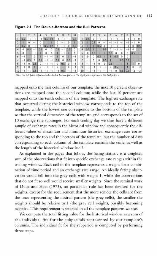
mapped onto the first column of our template; the next 10 percent observa-tions are mapped onto the second column; while the last 10 percent aremapped onto the tenth column of the template. The highest exchange ratethat occurred during the historical window corresponds to the top of thetemplate, while the lowest one corresponds to the bottom of the templateso that the vertical dimension of the template grid corresponds to the set of10 exchange rate subranges. For each trading day we thus have a differentsample of exchange rates in the historical window and consequently the dif-ferent values of maximum and minimum historical exchange rates corre-sponding to the top and the bottom of the template; but the number of dayscorresponding to each column of the template remains the same, as well asthe length of the historical window itself.
As explained in the pages that follow, the fitting statistic is a weightedsum of the observations that fit into specific exchange rate ranges within thetrading window. Each cell in the template represents a weight for a combi-nation of time period and an exchange rate range. An ideally fitting obser-vation would fall into the gray cells with weight 1, while the observationsthat do not fit so well would receive smaller weights. Since the seminal workof Duda and Hart (1973), no particular rule has been devised for theweights, except for the requirement that the more remote the cells are fromthe ones representing the desired pattern (the gray cells), the smaller theweights should be relative to 1 (the gray cell weight), possibly becomingnegative. This requirement is satisfied in all the template patterns we use.
We compute the total fitting value for the historical window as a sum ofthe individual f its for the subperiods represented by our template’scolumns. The individual fit for the subperiod is computed by performingthree steps.
chapter 9 TECHNICAL TR ADING RULES and winning 133
11
Note: The left pane represents the double bottom pattern. The right pane represents the bull pattern.
2 3 4 5 6 7 8 9 10
2345678910
11 2 3 4 5 6 7 8 9 10
0.5 1
1 1 0.5 0.5 1 1 1 0.5 0.5 0 1 1 1 1 1 1 1 01 0 1 0 1 1 0 1 0 1 1 0.5 0 1 1 1 1 1 1 0
0.5 0 1 0 0.5 0.5 0 1 0 0.5 1 1 0.5 0 1 1 1 1 0 0.50 0.5 1 0.5 0 0 0.5 1 0.5 0 0.5 1 1 0.5 0 1 1 1 0 10 1 1 1 0 0 1 1 1 0 0 0.5 1 1 0.5 0 0 0 0.5 1
1 1 0 1 1 1 1 0 1 1 0 0 0.5 1 1 0.5 0 0 1 11 0.5 0 0.5 1 1 0.5 0 0.5 1 1 0 0 0.5 1 1 0.5 0.5 1 11 0 0.5 0 1 1 0 0.5 0 1 1 1 0 0 0.5 1 1 1 1 01 0 1 0 1 1 0 1 0 1 1 1 1 1 0 0.5 1 1 0 21 1 0.5 1 1 1 1 0.5 1 1 1 1 1 1 1 0 0.5 0.5 2 3
2345678910
Figure 9.1 The Double-Bottom and the Bull Patterns
1. Compute the percentage of observations that falls into each one ofthe 10 subranges covered by the historical window.
2. Multiply these percentages by weights in the corresponding cells.
3. Sum the resulting 10 products to get the value of the fit for theparticular subperiod.
For example, if today we choose the historical trading window to be 100days and the exchange rate fluctuation range between 1 and 2 during thepast 100 days, each column in our template would correspond to a sub-period of 10 days with the first row of the template corresponding to therange of [1.9;2], the second one to [1.8;1.9] and the tenth row (which is the bottom row) corresponding to the range of [1;1.1]. If, for example, forthe past 100 days the exchange rate were fluctuating in the range of [1.9;2],then for each 10-day subperiod 100 percent of the observations would map into the upper row cell so that the value of the fit for each subperiodwould be simply equal to the template weight value, and the total fit for thehistorical window would be equal to the sum of the weights in the first rowof the template.
In this study we apply the trading window of 40 days, which is thelength used by the authors of studies that apply similar pattern recognitiontechniques (Leigh et al., 2002, and references therein). Regarding the fitting statistic, for each currency pair and the technical analysis pattern, weround the highest estimated fitting value down to the nearest integer.
Suppose we examine the performance of the bull trading rule in the case ofa EUR/USD currency pair. We determine the entry points by applying thepattern recognition techniques to the technical analysis patterns as describedabove. We then proceed by setting the stop-limit and stop-loss values. Let b bethe stop-limit value, while a is the stop-loss value. We proceed with the estimation of empirical probabilities of profitable entries as follows.
1. Given the sample of the observed exchange rates for EUR/USD( January 1, 1999 to January 31, 2007), identify points of entry basedon the bull pattern template from Figure 9.1 and the fitting statisticlevel (say, 7).
2. Compute the number of profitable entries, i.e., the ones that result inthe exchange rate deviating by points in the profit-making directionbefore deviating by a points in the loss-making direction. Call the
134 Part I i TECHNICAL TR ADING

share of such profitable entries Np. This will be our empiricalprobability of a profitable entry.
3. As follows from the weak-form EMH, the foreign exchangemovements are described by a simple random walk process, so thatthe share of profitable entries should approach NEMH
a—–—a b. The
latter follows from the fact that a simple random walk is a martingaleprocess (Williams, 1991). By computing Np s and NEHM s for alarge number of combinations of a and b, we can test whether theformer is statistically greater than the latter.
4. In case we find Np NEHM a—–—
a b for a particular trading rule andcurrency pair, the average expected empirical return on this rule isstatistically positive for this currency pair, since E[Rp] S [Np b
(1 Np) a] Rp is the empirical
return on a particular trading rule and a combination of stop-limitand stop-loss values.
We let a and b vary between 1 and 1,000 points with the increment of1 point, which supplys us with one million strategies for each currency pairand the technical analysis pattern (bull flag or double-bottom). The nextsection presents and discusses our empirical results.
EMPIRICAL RESULTS
In what follows, we use the following codenames for the currencies in oursample: EUR is euro, USD is the U.S. dollar, GBP is the British pound,NZD is the New Zealand dollar, CAD is the Canadian dollar, AUD is theAustralian dollar, CHF is the Swiss franc, and JPY is the Japanese yen. Whena technical analysis rule signals entry into the market, a currency pair is beingbought. For example, if a trader analyses the performance of euros versus U.S.dollars and deems euro is going to appreciate, she or he buys the EURUSDcurrency pair in the sense that the trader is buying euros for U.S. dollars.Below we present the differences between the empirical probabilities of real-izing positive returns by using technical analysis signals and the theoreticalones. We interpret positive differences as evidence of the technical analysisrules being able to increase the probability of realizing a positive return.
S b aa b
aa b
a× ×+
− −+
⎛
⎝⎜
⎞
⎠⎟ ×
⎡
⎣⎢
⎤
⎦⎥ =1 0.
chapter 9 TECHNICAL TR ADING RULES and winning 135

Since both a and b vary within the limits of 1 to 1,000, we have one million strategies for each currency pair and one of the two technical trad-ing patterns. We tested the extent to which the set of empirical probabilitiesof winning Np exceed their theoretical counterparts NEHM in the statisticalsense by employing a two-sample, one-tailed heteroscedastic t test. In all 20 cases, the estimated differences between empirical and theoretical prob-abilities proved to be statistically significant from zero, meaning the twotechnical rules we have been using are indeed causing a change in the prob-ability to win or to lose.
As evidenced by Table 9.1, in all but four cases, entering the marketaccording to one of the two technical trading rules does increase the proba-bility of winning. As mentioned in the Empirical Methodology section, thisis tantamount to realizing a positive return on a technical trading strategy.It is important to notice, however, that figures in Table 9.1 are not profitsper se, they are namely differences between empirical and theoretical prob-abilities of winning.
An interesting question is whether the results reported in Table 9.1 canbe of value to a practicing trader. In fact, the apparent ability of the twotechnical trading rules to increase the probability of beating the marketdoes not necessarily mean that one can identify a strategy that would uni-formly result in statistically positive returns.
In order to see whether one can identify such a strategy, we partition therange of stop-limit values b and stop-loss values a into 10 subranges each, andsee whether we can find a particular range of these values that uniformlyresults in a higher probability of winning relative to its theoretical counter-part. Table 9.2 below represents such a partition for the case of EURUSD andthe bull charting pattern. Sets of strategies resulting in positive differences
136 Part I i TECHNICAL TR ADING
Table 9.1 Differences Between Empirical and Theoretical Probabilities ofRealizing Positive Returns Due to Technical Analysis Application
EURUSD GBPUSD NZDUSD USDCAD AUDUSD
Bull 1.54% 21.78% 25.38% 11.41% 13.93%
Double-Bottom 38.93% 31.24% 14.96% 11.08% 1.07%
USDCHF USDJPY GBPJPY GBPUSD EURCHF
Bull 23.90% 25.00% 10.00% 17.62% 49.47%
Double-Bottom 26.15% 50.00% 25.00% 24.73% 25.38%

Table 9.2 Average Differences Between Empirical and Theoretical Probabilities of Winning for EURUSD, Bull Pattern
Limit (b)Stop (a) 100 200 300 400 500 600 700 800 900 1,000
100 50.00% 23.98% 16.14% 12.20% 9.81% 8.21% 7.06% 6.19% 5.51% 4.97%
200 37.30% 50.00% 37.40% 29.91% 24.93% 21.37% 18.71% 16.63% 14.98% 13.62%
300 39.86% 62.60% 50.00% 41.64% 35.69% 31.22% 27.76% 24.98% 22.71% 20.82%
400 43.80% 70.09% 58.36% 50.00% 43.74% 38.88% 34.99% 31.81% 29.16% 26.92%
500 46.19% 75.07% 64.31% 56.26% 50.00% 45.00% 40.90% 37.50% 34.61% 32.14%
600 10.83% 12.63% 2.78% 4.88% 11.00% 16.00% 20.17% 23.69% 26.72% 29.33%
700 7.06% 18.71% 27.76% 34.99% 40.90% 45.83% 50.00% 53.57% 56.67% 59.38%
800 6.19% 16.63% 24.98% 31.81% 37.50% 42.31% 46.43% 50.00% 53.13% 55.88%
900 5.51% 14.98% 22.71% 29.16% 34.61% 39.28% 43.33% 46.87% 50.00% 52.78%
1,000 4.97% 13.62% 20.82% 26.92% 32.14% 36.67% 40.62% 44.12% 47.22% 50.00%
Limit (b) and Stop (a) are the values of stop-limit and stop-loss orders. Bold figures represent ranges of these values.
137

between empirical and theoretical probabilities are shaded. Recall that, as evidenced by Table 9.1, the average difference between the empirical and the-oretical probabilities of winning is statistically negative for this case (i.e., forthe bull pattern in the case of the EURUSD currency pair).
We observe that in not an insignificant number of cases it is possible to realize a positive return by following a technical analysis strategy, forexample, by buying euros with U.S. dollars on the bull charting signal inFigure 9.1, and setting the stop-limit and stop-loss values to be 400 and600 points, respectively. However, after having inspected similar tables forall rules and currency pairs, we failed to discover any empirical regularityin the placement of positive numbered cells in those tables. In other words,we were unable to find a particular range or set of ranges of the stop-limitand stop-loss values that would result in a statistically positive increase inthe probability of winning for all currencies and both charting patterns.
Table 9.3 presents the cross-currency pair analysis of our strategies’ per-formance for the bull trading pattern. We look at the 10 subranges of bothstop-limit and stop-loss values and compute the average share of the numberof cases across the 10 currency pairs when the difference between empiricaland theoretical probabilities of winning is positive.
In 86 percent of the cells in Table 9.3 the values are above 50 percent,implying that the average return across currencies of the double-bottom
138 Part I i TECHNICAL TR ADING
Table 9.3 Share of Technical Trading Strategies Resulting in PositiveEmpirical Returns Across Currencies, Bull Pattern
Limit (b)Stop (a) 100 200 300 400 500 600 700 800 900 1,000
100 60% 60% 60% 60% 60% 60% 60% 50% 40% 40%
200 30% 60% 60% 60% 60% 60% 60% 50% 50% 40%
300 30% 50% 60% 60% 70% 70% 70% 60% 60% 50%
400 50% 60% 70% 70% 70% 70% 70% 60% 60% 50%
500 50% 50% 60% 70% 70% 70% 70% 60% 60% 60%
600 50% 50% 60% 70% 80% 80% 80% 70% 70% 70%
700 60% 60% 70% 70% 80% 80% 80% 70% 70% 70%
800 60% 60% 60% 70% 70% 80% 70% 70% 70% 60%
900 60% 60% 60% 70% 70% 60% 70% 70% 60% 60%
1,000 60% 60% 60% 70% 70% 60% 60% 70% 60% 40%
Limit (b) and Stop (a) are the values of stop-limit and stop-loss orders. Bold figures represent ranges of thesevalues.

trading rule for the corresponding range of stop-limit and stop-loss valuesis predominantly statistically positive. We computed a similar table for thebull flag trading rule and observed the same predominance of the money-making strategies over the loss-making ones (90 percent of the cells).
Finally, the regression analysis (results available immediately uponrequest) for the individual currency pairs did not reveal any robust relation-ship between winning probability increases and stop-limit and stop-loss val-ues for neither trading rule and the currency pairs either, leading us tobelieve that it is indeed hard to find a universally working strategy even ifthe technical rules appear to be working on average across currency pairsand the stop-limit and stop-loss parameters.
CONCLUSION
In this study we examined the ability of two technical analysis rules,namely, the bull and double-bottom pattern, to increase the probability ofwinning in the foreign exchange market relative to the theoretical probabil-ity. The latter was computed on the basis of the efficient market hypothesis,implying, among other things, that foreign exchange rates follow a simplerandom walk.
In the course of our analysis we tested one million strategies for theworld’s 10 major currency pairs on the dataset covering eight years, whichallows us to formulate two stylized facts that simultaneously demonstratethe technical analysis’ potential for profitability, and the difficulty of itspractical application:
1. The bull and double-bottom technical analysis rules increase onaverage the probability of winning compared to what is stipulated bythe efficient market hypothesis.
2. It is hardly possible to indicate a strategy in terms of the trading ruleand a combination of stop-loss and stop-limit values, which wouldconsistently result in statistically positive profits in the case of allcurrency pairs.
The two stylized facts above help explain the persistent popularity oftechnical analysis rules among popular traders on the one hand and lack ofthe “sure-fire” trading strategies on the other hand (otherwise, everyonewould be a millionaire!). Indeed, while technical analysis appears to be
chapter 9 TECHNICAL TR ADING RULES and winning 139

increasing the probability of winning, the lack of systemic pattern in thewinning strategies’ parameters and underlying technical trading rules makesit difficult, if not impossible, to use technical analysis for reaping consistentpositive returns.
REFERENCES
Bae, K.H., Jang, H., and Park, K.S. (2003) Traders’ Choice between Limitand Market Orders: Evidence from NYSE Stocks. Journal of FinancialMarkets, 6(4): 517–538.
Duda, R. and Hart, P. (1973) Pattern Classification and Scene Analysis. NewYork: John Wiley & Sons.
Fama, E.F. (1970) Efficient Capital Markets: A Review of Theory and Empir-ical Work. Journal of Finance, 25(2): 383–417.
Leigh, W., Modani, N., Purvis, R., and Roberts, T. (2002) Stock MarketTrading Rule Discovery using Technical Charting Heuristics. ExpertSystems with Applications, 23(2): 155–159.
Luca, C. (2000) Trading in the Global Currency Markets. New York: NewYork Institute of Finance.
Menkhoff, L. and Taylor, M.P. (2007) The Obstinate Passion of ForeignExchange Professionals: Technical Analysis. Journal of Economic Litera-ture, 45(4): 936–972.
Osler, C.L. (2005). Stop-loss Orders and Price Cascades in Currency Markets. Journal of International Money and Finance, 24(2): 219–241.
Williams, D. (1991) Probability with Martingales. Cambridge, UK: CambridgeUniversity Press.
140 Part I i TECHNICAL TR ADING

141
10C H A P T E R
Technical Analysisin TurbulentFinancial MarketsDoes Nonlinearity Assist?
Mohamed El Hedi Arouri, Fredj Jawadi, and Duc Khuong Nguyen
ABSTRACT
Along with the existence of financial markets, financial practitioners andacademic researchers are always concerned by the question of whether wecan forecast the future path of stock returns. In theory, if financial marketsare not fully efficient under the weak-form as defined by Fama (1970),investors can generate abnormal profits by performing technical analysisbased on past price and trading volume data. A comparison of the predic-tive power between competitive models shows that technical trading toolscommonly used might not be valid and effective in turbulent times such asextreme events and financial crisis due explicitly to the assumption of lineardependences in stock returns. At the empirical level, we first apply com-monly used chartist tools to empirically study and forecast stock returnsfrom actual data. These models are then extended to nonlinear frameworkand employed to test for the contribution of nonlinearity in modeling stockreturns. Using intraday data from two developed markets (France and Germany), we point out the superiority of nonlinear models and the contri-bution of nonlinearity-enhanced technical models over the linear tools,especially when stock returns are subject to structural changes.

INTRODUCTION
As long as financial markets exist, investors and portfolio managers attemptto make forecasts about the future asset prices based on the latter’s pastpatterns. The hope is then to establish trading rules that render theirinvestments profitable. For many peoples, the question in financial practiceis not whether it is possible to forecast the future path of asset prices, buthow to efficiently forecast it. Of the techniques used to recommend “buy”or “sell” signals based on an investigation of the predictability of pricechanges, the technical analysis has received less academic attention albeit itis widely employed by practitioners.1
In theory, the use of technical analysis will have no value if financialmarkets are at least weak-form efficient since in this case future pricemovements cannot be predicted using past price movements (Fama, 1970,1991). Empirical research is, however, not conclusive on the usefulness ofsuch trading rules. On the one hand, a number of studies find that technicalanalysis is unable to reliably predict future returns (Fama and Blume, 1966;Jensen and Bennington, 1970; Marshall and Cahan, 2005; Marshall, Cahan,and Cahan, 2008). For example, the study of Marshall et al. (2008) showsno evidence that technical trading rules are profitable using 5-minute rawand squared return series in the U.S. equity markets after the bootstrapmethodology is employed to correct for the potential of data snoopingbias.2 Using the similar approach, Marshall and Cahan (2005) reject thevalidity of technical analysis for the stock market in New Zealand eventhough the latter displays symptoms of an inefficient market such as smallnature, short-selling constraints, and lack of insider trading regulation.Other studies also report that technical analysis is not profitable once trans-action costs are considered (e.g., Allen and Karjalainen, 1999; Olson, 2004).
There is, on the other hand, a considerable amount of evidence to sug-gest that stock returns display short-term momentum profits and as a resultthe use of technical trading rules may lead to economically significantexcess returns in financial markets (e.g., Brock, Lakonishok, and LeBaron,1992; Corrado and Lee, 1992; Bessembinder and Chan, 1995; Hudson,Dempsey, and Keasey, 1996; Detry and Gregoire, 2001; Lee et al., 2003).More precisely, Brock et al. (1992) provide evidence that a relatively simpleset of technical trading rules has predictive power for changes in the DowJones Industrial Average, while empirical results of subsequent studies areconsistent with profitable technical analysis in European and Asian equity
142 Part i I TECHNICAL TR ADING

markets. Overall, past price movements and price trends may still have themerits in forecasting the future price changes, and technical trading rulessuch as moving averages, standard filter rules, and trading range break havebecome standard technical indicators in financial practice.
This chapter joins the previous studies by reinvestigating the effective-ness of technical trading rules in two major developed markets, Germanyand France, using intraday data. We contribute to the related literature inthat we introduce nonlinearities into traditional linear technical models tocapture any nonlinear dependence and adjustment in the past price changes.At the same time, our approach permits to examine the usefulness of tech-nical analysis in financial market turbulences, which has rarely been thefocus of previous work. Our motivations come essentially from the fact thatthe presence of numerous market distortions during crisis times may lead tononlinear forms of price dependence. The obtained results from estimatingnonlinearity-enhanced models confirm effectively our basic intuition thatnonlinearities do improve the effectiveness of technical analysis, especiallyduring episodes of widespread market panics.
The remainder of the chapter is organized as follows: the second sectionof this chapter outlines the reasons for which nonlinearities are introducedinto technical trading rules to test for the effectiveness of technical analysisagainst market efficiency. This chapter’s third section describes data usedand discusses empirical results. Summary conclusions are provided in thischapter’s final section.
NONLINEAR MODELING FOR TECHNICAL ANALYSIS
The succession of financial crises over the past two decades such as thestock crash in 1987, the Asian financial crisis in 1997, the Internet bubblecollapse in 2000, and more recently the current global financial crisis in2007 to 2009 has generated widespread market panics and pointed out theweakness of the usual financial analysis and modeling techniques in fore-casting the dynamic of financial markets. For example, technical analysisseems to be relevant only in the short term and may not yield good predic-tions when markets pass through financial turbulences and crises. Afterbriefly discussing the economic justifications of nonlinearity for financialmarkets, we discuss the appropriate nonlinear models to further test theeffectiveness of technical trading rules in turbulent financial markets.
chapter 10 TECHNICAL A NALYSIS IN TURBULENT Markets 143

Nonlinearity and Stock Market Dynamics
The financial literature has advanced several microeconomic and macro-economic justifications for the introduction of nonlinearity in modelingfinancial market dynamics. Regarding microeconomic explanations, oneshould note transaction costs (Dumas, 1992; Anderson, 1997), informationasymmetry (Artus, 1995), behavioral heterogeneity (De Grauwe andGrimaldi, 2005; Boswijk, Hommes, and Manzan, 2007), and mimeticbehavior (Orléan, 1990) that are suggested to be the main sources ofnonlinearity, structural breaks, and changes in asset price dynamics. Froma macroeconomic view, Artus (1995) show that the naissance and withdrawof speculative bubbles may induce asymmetric and nonlinear dynamics infinancial price dynamics.
Empirically, Gouriéroux, Scaillet, and Szafarz (1997) suggest that besidethe fact that financial markets are naturally and theoretically characterizedby nonlinear dynamics, the tools used to model stock price dynamics shouldcapture nonlinearity. The authors identify five types of nonlinearity. First,nonlinearity may take root in predicted variables. For example, to evaluatethe risk of a financial asset, we forecast its squared return which is a nonlin-ear variable. Second, nonlinearity is directly incorporated into forecastingtools used to predict future dynamics of price. Third, nonlinearity is pres-ent in the model parameters and is apprehended through the rejection ofthe normality for almost all financial series. Fourth, nonlinearity character-izing the price dynamics may be due to the presence of nonlinear relation-ships between past and present realizations of financial series (e.g., series ofstock returns). This type of nonlinearity can be present either in the meanor in the variance of the series under consideration or both. Finally, the lasttype of nonlinearity is inherent to financial strategies adopted by investorsin order to optimize the risk-return tradeoff.
Nonlinear Models
Several nonlinear models have been used in recent years to reproduce thedynamics of financial markets. Indeed, financial return dynamics are oftenmodeled by using the so-called regime-switching models while generalizedautoregressive conditional heteroscedasticity class models are rather appliedto conditionally evaluate return volatility. Among these nonlinear models,we focus on nonlinear models in mean and particularly on bilinear (BL) andnonlinear moving average (NMA) models that will be applied to intraday
144 Part i I TECHNICAL TR ADING

stock data at the empirical stage. Compared to previous studies on nonlin-ear stock price dynamics, our empirical investigation has two advantages.On the one hand, the use of these nonlinear models enables to appropri-ately extend the usual models of technical analysis (e.g., moving averagemodel and smoothing model) to a nonlinear context. On the other hand,their applications to intraday data would enhance the predictive power ofthe models used since this analysis appears to be particularly accurate in theshort term.
Bilinear Models (BL)
The BL models were introduced by Granger and Anderson (1978). Theirmodeling techniques and different specifications such as stochastic BL anddeterminist BL are rigorously presented in Guégan (1994). BL models con-stitute an extension for autoregressive moving average (ARMA) models byadding both compounded AR and MA terms to a traditional ARMA model.The nonlinearity of BL models is then introduced through these com-pounded terms. It is worth noting that BL models are generally recom-mended for reproducing the dynamics of financial series with periods of highvolatility followed by phases of lower volatility. Such dynamics characterizefinancial markets particularly when they pass through turbulent phases.
Let Yt be described by a BL process of (p, q, P, Q) orders, then itsdynamics can be defined as follows:
(10.1)
where εt is an error term, and αi, βj, and δkl belong to 3. If P Q, the BLmodel is said to be upper-diagonal, under-diagonal for P Q, and diagonalfor P Q. Assuming that εt → N(0, σ2
ε) and Yt is inversible, i.e., we canwrite εt f (Yt, Yt 1, …), BL models can be estimated using a proceduresimilar to that of Box and Jenkins (1970).3 It means that modeling steps thatwe usually employ for dealing with ARMA models (i.e., specification anddetermination of lag number, estimation, validation, and prediction) are alsoapplicable to BL models. However, it is commonly advised to test the nullhypothesis of linearity against its alternative of nonlinearity in order to correctly specify the BL models. The Saikkonen and Luukkonen (1991)test, which contains three main steps below, can be used to test for therobustness of BL models.
chapter 10 TECHNICAL A NALYSIS IN TURBULENT Markets 145
Y Y Yt i t ii
p
j t jj
q
k
P
k l t k t l= + +−=
−= =
− −∑ ∑ ∑α β ε δ ε1 1 1 ll
Q
t=
∑ +1
ε

• Step 1: We estimate a usual AR(p) model, retain the estimatedresidual εt and compute the sum of squared residuals (SSR) under thenull hypothesis
• Step 2: We estimate the following regression
and we compute
• Step 3: We compute the statistics where T
denotes the observation number associated with the regression of the
second step. Under the null hypothesis of linearity, the statistic BL is
distributed as a χ2 with (P Q) degrees of freedom.
BL models were used only in some studies such as Subba Rao and Gabr(1984), Chan and Tong (1986).4
Nonlinear Moving Average (NMA) Models
NMA models were introduced by Robinson (1977). These models arebased on Volterra developments and are defined as5
(10.2)
where εt is a white noise and θ0 is equal to 1. NMA models are estimated bythe method of moments, but their practical application in economics andfinance is somewhat limited. In practice, Robinson (1977) has recom-mended a NLM model of order one as in Equation 10.3 to capture theasymmetry characterizing business cycles with gradual expansion andabrupt recession. The NLM model is accordingly suitable for modeling thedynamics of financial markets whose evolution also displays high degree ofasymmetric patterns.
(10.3)
The asymmetry is captured through the term, εt1 εt2, while the fore-casting of positive and negative phases is reproduced depending on the
BL TSSR SSR
SSR=
−0 1
0
,
SSR ti
T
12
1
==
∑ν+ +=
− −=
∑ ∑k
P
k l t k t ll
Q
tY1 1
δ ε ν
ε α β εt i t ii
p
j t jj
q
Y= +−=
−=
∑ ∑1 1
SSR ti
T
02
1
==
∑ε
146 Part i I TECHNICAL TR ADING
Yt i t ii
q
i
q
i j t i t jj
q
i
q
j
= + +−= =
− −= =
∑ ∑ ∑ ∑θ ε θ ε ε0 0 0 0 ==
− − −=
∑ ∑ +0 0
q
i j k t i t j t kk
q
θ ε ε ε
Yt t t t t= + +− − −ε θ ε θ ε ε1 1 2 1 2

sign of εt and through the observations εt, εt 1 εt 2, . . . and εt, εt1
εt2, . . ., respectively.
DATA AND EMPIRICAL RESULTS
Data and Preliminary Results
Previous studies that focus on technical trading rules show that the analysisis particularly appropriate in the short term using high frequency data. Forcomparative purpose, we employ, in our empirical application, intradaystock price data of two developed countries: France (CAC 40) and Germany (DAX 30). The use of intraday data permits to test the instanta-neous adjustment dynamics of stock markets. Our data, consisting offive-minute prices obtained from Euronext database, cover the period fromJanuary 2, 2007 to April 22, 2009 in order to test the effectiveness of tech-nical analysis during the financial crisis.
To start, we check the stationarity of our variables using Dickey-Fuller,Philips-Perron, and KPSS unit root tests. The hypothesis of unit root isrejected only for the series in the first difference, indicating that bothindexes are integrated of order one, I(1).6 We then focus on stock returnsdefined as the first difference of stock prices expressed in logarithm.
The investigation of descriptive statistics of French and German stockmarket intraday returns, reported in Table 10.1, provides evidence of strongrejection of the symmetry and normality hypotheses. It also shows somevolatility excess and autoregressive conditional heteroscedasticity effects inFrench and German stock returns. These findings indicate a priori some evidence of nonlinearity and asymmetry characterizing stock price dynamics.
To check the validity of technical analysis, we will first estimate usual linear models, and then we examine whether the introduction of nonlinearitycontributes to improve the forecasting power of technical analysis.
chapter 10 TECHNICAL A NALYSIS IN TURBULENT Markets 147
Table 10.1 Descriptive Statistics
ARCHMean SD Skewness Kurtosis Jarque–Bera (q) No. of obs.
RF 1.31E05 0.0015 0.161 19.51 65,5373.0 6762.7 (15) 57,710
RG 4.74E06 0.0015 0.184 24.53 111,4553.0 8600.9 (16) 57,710
RF, French stock returns; RG, German stock returns; SD, standard deviation; ARCH, autoregressiveconditional heteroscedasticity.
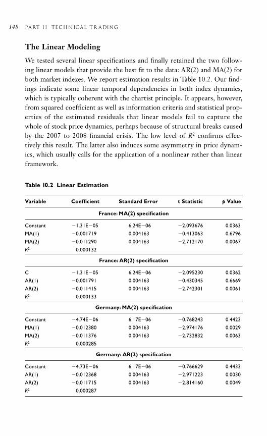
148 Part i I TECHNICAL TR ADING
The Linear Modeling
We tested several linear specifications and finally retained the two follow-ing linear models that provide the best fit to the data: AR(2) and MA(2) forboth market indexes. We report estimation results in Table 10.2. Our find-ings indicate some linear temporal dependencies in both index dynamics,which is typically coherent with the chartist principle. It appears, however,from squared coefficient as well as information criteria and statistical prop-erties of the estimated residuals that linear models fail to capture thewhole of stock price dynamics, perhaps because of structural breaks causedby the 2007 to 2008 financial crisis. The low level of R2 confirms effec-tively this result. The latter also induces some asymmetry in price dynam-ics, which usually calls for the application of a nonlinear rather than linearframework.
Table 10.2 Linear Estimation
Variable Coefficient Standard Error t Statistic p Value
France: MA(2) specification
Constant 1.31E05 6.24E06 2.093676 0.0363
MA(1) 0.001719 0.004163 0.413063 0.6796
MA(2) 0.011290 0.004163 2.712170 0.0067
R2 0.000132
France: AR(2) specification
C 1.31E05 6.24E06 2.095230 0.0362
AR(1) 0.001791 0.004163 0.430345 0.6669
AR(2) 0.011415 0.004163 2.742301 0.0061
R2 0.000133
Germany: MA(2) specification
Constant 4.74E06 6.17E06 0.768243 0.4423
MA(1) 0.012380 0.004163 2.974176 0.0029
MA(2) 0.011376 0.004163 2.732832 0.0063
R2 0.000285
Germany: AR(2) specification
Constant 4.73E06 6.17E06 0.766629 0.4433
AR(1) 0.012368 0.004163 2.971223 0.0030
AR(2) 0.011715 0.004163 2.814160 0.0049
R2 0.000287

Nonlinear Modeling for Technical Analysis
First of all, the linearity is tested using Saikkonen and Luukkonen (1991)test. Then BL and NMA models are estimated. The most important find-ings are reported in Table 10.3 and Table 10.4. The linearity is rejected for
chapter 10 TECHNICAL A NALYSIS IN TURBULENT Markets 149
Table 10.3 Linearity Test of Saikkonenand Luukkonen (1991)
France Germany
BL 10.3 7.72
(p value) (0.03) (0.10)
Table 10.4 Nonlinear Estimation Results
France Germany
BL model
α1 0.21 0.87[0.21] [0.49]
α2 0.06 0.36[2.3] [1.81]
β1 0.24 0.91[0.20] [0.52]
β2 0.08 0.39[1.67] [1.75]
δ11 5.4 0.35[1.93] [1.13]
δ22 0.65 [2.58][2.3] 0.70
R–2 0.11 0.07
DW 2.0 2.01
NRNL (p value) 0.04 0.03
NMA model
θ1 0.03 0.05[2.35] [4.16]
θ11 0.37 0.08[4.57] [2.76]
R–2 0.55 0.45
DW 2.1 1.86
NRNL (p value) 0.38 0.23
NRNL designates the p value for no-remaining nonlinearity.Values between [.] denote the t statistics.
the French market index at the statistical level of 5 percent, while it isrejected for German market index only at the 10 percent level.
For both indexes, the specification tests lead to choose a BL(2,2,2,2) andNMA of one order that we estimate by the maximum likelihood method.According to our findings, BL models seem not to capture the whole non-linearity characterizing our data (NRNL test), even though nonlinear termsare statistically significant. NMA models seem however to be more appro-priate to capture the asymmetry inherent to French and German stockmarket dynamics. Indeed, their estimators are statistically significant andthey seem to have apprehended all nonlinearity inherent to stock returnsunder consideration. In addition, the negativity of their coefficients indi-cates that French and German indexes are still undervalued and that mar-kets are in phase of correction.
Otherwise, the validation of a NMA model to reproduce these stockreturn dynamics indicates a nonlinear time-varying dependency in stockreturns. This is consistent with profitable technical analysis, but suggests anextension of the usual tools to a nonlinear framework to improve the fore-casting accuracy.
CONCLUSION
In this chapter, we have examined the effectiveness of technical tradingrules in two major developed markets, the German and French stock mar-kets, using intraday data. We have used both linear and nonlinear technicalanalysis models. The usefulness of nonlinear models is justified by manyfactors, in particular, the presence of numerous market distortions such asinformation and transaction costs, asymmetries, investor’s heterogeneity,and structural changes during financial crisis. Our empirical findings con-firm effectively our basic intuition that nonlinearities do improve the effec-tiveness of technical analysis, especially during episodes of widespreadmarket panics.
REFERENCES
Allen, F. and Karjalainen, R. (1999) Using Genetic Algorithms to FindTechnical Trading Rules. Journal of Financial Economics, 51(2):245–271.
150 Part i I TECHNICAL TR ADING

Anderson, H.M. (1997) Transaction Costs and Nonlinear Adjustmenttowards Equilibrium in the US Treasury Bill Markets. Oxford Bulletinof Economics and Statistics, 59(4): 465–484.
Artus, P. (1995). Anomalies sur les Marchés Financiers. Paris: EditionsEconomica.
Bessembinder, H. and Chan, K. (1998) Market Efficiency and the Returnsto Technical Analysis. Financial Management, 27(2): 5–13.
Boswijk, H.P., Hommes, C.H., and S. Manzan. (2007) Behavioral Hetero-geneity in Stock Prices. Journal of Economic Dynamics and Control,31(6): 1938–1970.
Box, G. and Jenkins, G. (1970) Time Series Analysis: Forecasting and Control,San Francisco: Holden-Day.
Brillinger, D.R. (1970) The Identification of Polynomial Systems by Meansof Higher Order Spectra. Journal of Sound and Vibration, 12 (3):301–313.
Brock, W., Lakonishok, J., and LeBaron, B. (1992) Simple Technical Trading Rules and the Stochastic Properties of Stock Returns. Journalof Finance, 48(5): 1731–1764.
Chan, K.S. and Tong, H. (1986) On Estimating Thresholds in AutoregressiveModels. Journal of Time Series Analysis, 7(3): 179–190.
Chan, K.S., Moeanaddin, R., and Tong, H. (1988) Some Difficulties ofNonlinear Time Series Modelling. Technical report, University ofManchester, UK.
Corrado, C.J. and Lee, S.H. (1992) Filter Rule Tests of the Economic Significance of Serial Dependence in Daily Stock Returns. Journal ofFinancial Research, 15(4): 369–387.
De Grauwe P. and Grimaldi M. (2005) Heterogeneity of Agents, TransactionCosts and the Exchange Rate. Journal of Economic Dynamics and Control,29(4): 691–719.
Detry, P.J. and Gregoire, P. (2001) Other Evidence of the Predictive Powerof Technical analysis: the Moving Average Rules on European Indices.Working paper, University of Namur, Belgium.
Dumas, B. (1992) Dynamic Equilibrium and the Real Exchange Rate in aSpatially Separated World. Review of Financial Studies, 5(2): 153–180.
chapter 10 TECHNICAL A NALYSIS IN TURBULENT Markets 151

Fama, E.F. (1970) Efficient Capital Markets: a Review of Theory andEmpirical Work. Journal of Finance, 25(2): 383–417.
Fama, E.F. (1991) Efficient Capital Markets. Journal of Finance, 46(5):1575–1617.
Fama, E.F. and Blume, M. (1966) Filter Rules and Stock Market Trading.Journal of Business, 39(1): 226–241.
Gouriéroux, C., Scaillet, O., and Szafarz, A. (1997). Econométrie de laFinance. Paris: Editions Economica.
Granger, C.W. J. and Anderson, A.P. (1978). An Introduction to BilinearTime Series Analysis. Gottingen, Germany: Vandenhoeck and Rupecht.
Guégan, D. (1994). Séries Chronologiques Non-Linéaires a Temps Discret.Paris: Editions Economica.
Hudson, R., Dempsey, H., and Keasey, K. (1996) A Note on Weak FormEfficiency of Capital Markets: the Application of Simple TechnicalTrading Rules to UK Prices 1935–1994. Journal of Banking Finance,20(6): 1121–1132.
Jensen, M.J. and Bennington, G. (1970) Random Walks and Technical Theories: Some Additional Evidence. Journal of Finance, 25(2):469–482.
Lee, D.D., Chan, H., Faff, R.W., and Kalev, P.S. (2003) Short-term Con-trarian Investing—It is Profitable—Yes and No. Journal of MultinationalFinancial Management, 13(4–5): 385–404.
Marshall, B.R. and Cahan, R.H. (2005) Is Technical Analysis Profitable ona Stock Market Which Has Characteristics that Suggest It May beInefficient? Research in International Business and Finance, 19(3):384–398.
Marshall, B.R., Cahan, R.H., and Cahan, J.M. (2008) Does Intraday Tech-nical Analysis in the US Equity Market Have Value? Journal of Empiri-cal Finance, 15(2): 199–210.
Olson, D. (2004) Have Trading Rule Profits in the Currency MarketsDeclined Over Time? Journal of Banking and Finance, 28(1): 85–105.
Orléan A. (1990) Le Rôle des Influences Interpersonnelles dans la Détermi-nation des Cours Boursiers. Revue économique, 41(5): 839–868.
Robinson, P.M. (1977) The Estimation of a Nonlinear Moving AverageModels. Stochastic Processes and Their Applications, 5(1): 81–90.
152 Part i I TECHNICAL TR ADING

Saikkonen, P. and Luukkonen, R. (1991) Power Properties of Time SeriesLinearity Test against Some Simple Bilinear Alternatives. StatisticaSinica, 1(2): 453–464.
Subba Rao, T. and Gabr, M.M. (1984). An Introduction to BispectralAnalysis and Bilinear Time Series Models. Lecture Notes in Statistics.New York: Springer Verlag.
NOTES
1. Marshall, Cahan, and Cahan (2008) note that market participants andjournalists consistently attach, according to the results obtained fromsurveys, more emphasis on technical analysis than on fundamentalanalysis as far as the short-term forecast horizon is concerned. In partic-ular, the respondents give approximately twice as much weight on technical analysis for intraday horizons as they do for one-year horizons.
2. The bootstrap methodology was introduced to finance literature byBrock, Lakonishok, and LeBaron (1992) and has become popular forassessing the statistical significance of technical trading rule profitabil-ity. It consists of comparing conditional buy or sell signal using theoriginal return series with conditional buy or sell signal generated fromthe corresponding simulated series using specified technical analysismodels such as moving average, random walk, AR(1), GARCH-M, andEGARCH. Note that, to obtain the bootstrap results, the initial sampleis simulated n times (n sufficiently large, i.e., n is usually higher than1,000) by resampling with replacement so that the usual normal distri-bution needs not to be assumed for the model residuals.
3. See Guégan (1994) for more details concerning other estimation meth-ods for BL models such as the method of moments.
4. See Chan, Moeanaddin, and Tong (1988) for more details regarding theproblems and limitations associated with BL modeling.
5. See Wiener (1958) and Brillinger (1970) for more details aboutVolterra developments and their statistical properties.
6. Results of unit root tests are available upon request to the correspondingauthor.
chapter 10 TECHNICAL A NALYSIS IN TURBULENT Markets 153

This page intentionally left blank

155
11C H A P T E R
Profiting from theDual-MovingAverage Crossoverwith ExponentialSmoothing
Camillo Lento
ABSTRACT
This chapter reexamines the profitability of the dual-moving averagecrossover trading rule by analyzing the incremental profit contribution ofutilizing an exponential smoothing technique to calculate the moving aver-ages. The analysis is conducted on the S&P 500, NASDAQ, and Dow JonesIndustrial Average from January 1999 to April 2009 (N 2,596). Theresults suggest that the profitability of the moving average cross-over rule issignificantly enhanced by using an exponential smoothing technique thatreduces the weight of the most recent price observation. The additionalprofits are not the result of increased risk. Rather, exponentially smoothingprices to calculate the moving averages results in a fewer number of signalsthat are more informative. Bootstrapping simulations were used to test forsignificance.

INTRODUCTION
The dual-moving average crossover (DMACO) trading strategy is one ofthe simplest, yet most popular trading rules among practitioners (Taylorand Allen, 1992; Lui and Mole, 1998). It is one of the few trading rules thatis statistically well defined (Neftci, 1991). The DMACO is calculated withtwo moving averages of a security price. Relative to each other, one movingaverage is short term (STMA), while the other long term (LTMA). TheLTMA will move in the same direction as the STMA, but will have a lowervariance and move at a slower rate. The different rate of direction createssituations where the values of the two moving averages may equal orcrossover one another. These crossover points generate buy and sell signalsunder the DMACO. A buy signals occurs when the STMA rises above theLTMA, whereas a sell signal occurs when the STMA breaks below theLTMA (Murphy, 2000).
Various studies have tested the profitability of technical trading rules(e.g., Bessembinder and Chan, 1998; Lo, Mamaysky, and Wang, 2000;Lento, 2008). This chapter provides new insights on the profitability andsign prediction ability of the DMACO by utilizing an exponential smooth-ing technique to calculate the STMA and LTMA. Traditionally, the latestprices are of the most value to an exponentially smoothed average. How-ever, this study utilizes a smoothing technique that places more weight onthe older values.
The trading rules are tested on the S&P 500, NASDAQ, and DowJones Industrial Average (DJIA) for the period January 1999 to April 2009(N 2,596). The results suggest that the profitability of DMACO is sig-nificantly enhanced when the STMA and LTMA are calculated with theexponential smoothing technique. The increased profitability is signifi-cant, in many cases in excess of 5.0 percent per annum, and consistentacross each moving average combination and index. Profitability is definedas returns in excess of the naïve buy-and-hold trading strategy.
The additional profits are not the result of increased risk. Rather, expo-nentially smoothing prices to calculate the moving averages results in afewer number of signals that are more informative. The results from thesign prediction tests are consistent with the profitability tests as large, posi-tive returns followed the buy signal of the exponentially smoothed DMACO
The remainder of this chapter is organized as follows: the next sectiondescribes the DMACO. The third section of this chapter describes the
156 Part I i TECHNICAL TR ADING
data, while the fourth section explains the methodology. This chapter’sfifth section presents the results, and a conclusion is provided in the finalsection.
BACKGROUND ON THE MOVING AVERAGES
The Dual-Moving Average Crossover Trading Rule
The DMACO produces a buy (sell) signal when the STMA cuts the LTMAfrom below (above). The simple rule has a large variety of forms based onthe timeframe selected for each average (Neely, Weller, and Dittmar, 1997).The intuition behind the DMACO can be explained in terms of momen-tum. When SMTA is greater than the LTMA, the security’s value in therecent past exceeds its value in the more distant past, which in moving aver-age models signals that an upward trend is developing (Levich, 2001).When the STMA moves below the LTMA, this provides a lagged indicatorthat the price is moving downward relative to the historical price.
There are two variants of the DMACO trading rule: variable lengthmoving average (VMA), and the fixed-length moving average (FMA). TheVMA generates a buy (sell) signal whenever the STMA is above (below) theLTMA. After a buy (sell) signal, the investor will be long (out of ) the mar-ket until a sell (buy) signal is generated. Conversely, the FMA focuses solelyon the crossing of the moving averages. This method stresses that thereturns should be different for a few days following a crossover (Brock,Lakonishok, and LeBaron, 1992).
Empirical Tests of DMACO Trading Rule1
There are many studies on moving average rules. Brock et al. (1992) wasone of the most influential, and found that returns generated from thesignals of a DMACO rule outperformed three popular models (AR(1),GARCH-M, and the exponential GARCH). Buy signals resulted inhigher returns than sell signals, and displayed less volatility than the sellsignal returns.
Levich and Thomas (1993) also tested moving average rules to evaluatethe potential for abnormal profits. Their study suggests that the DMACOgenerated excess returns that would have been highly unlikely to have beenobserved by chance.
chapter 11 Profiting from the Dual-Moving Average 157
Gençay and Stengos (1998) tested a 50-day and a 200-day DMACO.Linear and nonlinear models were used to assess the predictability the sig-nals on the daily DJIA from 1897 to 1988. The results provide evidence ofa 10 percent (or better) forecasting improvement during the GreatDepression years and in the years 1980 to1988. The technical tradingrules provided more moderate returns during the period 1939 to 1950.Gençay (1999) corroborated the significance of moving average rules as atool to predict foreign exchange rates. He concluded that simple movingaverage rules provide significant correct signals and returns.
However, the literature does not provide consensus support for the prof-itability of the DMACO. For example, Kho (1996) presents a contraryviewpoint by supporting the ineffectiveness of technical trading rules bysuggesting that time-varying risk premiums can explain a substantialamount of the profitability of DMACO in foreign currency markets.
Recent research reveals that DMACO is profitable in certain Asianequity markets (Lento, 2007). The DMACO trading rule was profitable in22 of the 24 (91.7 percent) tests. The 1-day, 50-day DMACO performedthe best as all nine variants tested outperformed the buy-and-hold tradingstrategy as it earned annual excess returns in the range of 1.8 percent to32.6 percent. The 1-day, 200-day DMACO also earned annual excessreturns in the range of 1.5 percent to 10.9 percent.
Exponential Smoothing and Moving Averages
A moving average relies equally on past observations (i.e., the weightassigned to the observations are the same and equal to 1/N). Exponentialsmoothing assigns exponentially decreasing weights to older observations. In other words, recent observations are given relatively more weight in fore-casting than older observations. There is one or more smoothing parameterto be determined (or estimated) in exponential smoothing and thesechoices determine the weights assigned to the observations (Hyndman et al., 2008).
Exponential smoothing has been used in technical trading rules. Forexample, the triple exponential smoothing oscillator (TRIX) was developedby John Hutson, while Gerald Appel developed the moving average conver-gence/divergence (MACD). Although exponential smoothing is used inpractice to develop trading rules, little academic research exists that teststhe profitability of exponential smoothing techniques. Specifically, there is
158 Part I i TECHNICAL TR ADING

no known research that tests whether exponential smoothing can increasethe profitability and sign prediction ability of the DMACO. This chapterhelps to fill this gap in the literature.
METHODOLOGY
Calculating the Dual-Moving Average Crossover TradingSignals
As discussed, the DMACO generates a buy (sell) signal whenever theSTMA is above (below) the LTMA as follows:
Buy Signal Equation
(11.1)
Sell Signal Equation
(11.2)
where Ri,t is the average security price given the number of days that definesthe STMA, and is Ri,t1 the average price over the number of days thedefines the LTMA.
Traditionally, the STMA and LTMA are calculated with the securityprice time-series. The moving averages in this study are calculated with anexponentially smoothed security price-time series. The smoothing schemeemploys the single exponential smoothing methodology and begins by defin-ing S2 to y1, where Si stands for smoothed observation, and y stands for theoriginal security price. The subscripts refer to the time periods, 1, 2, …, n.For the third period, S3 y2 (1 – ) S2. The smoothed series starts withthe smoothed version of the second observation (i.e., there is no S1). For anytime period t, the smoothed value St is found by computing:
(11.3)
where parameter is the smoothing constant. Normally, α is set to greaterthan 50 percent to allow for more weight on the more recent observation.However, this study utilizes an α of 10 percent, thereby placing significantly
chapter 11 Profiting from the Dual-Moving Average 159
R
S
R
LBuy
i ts
S
i tl
L
, ,== −−==∑∑ ∑∑>> ==1 11
R
S
R
LSell
i ts
S
i tl
L
, ,== −−==∑∑ ∑∑<< ==1 11
S y S o tt t t== ++ −− << ≤≤ ≥≥−− −−α α α1 11 1 3( )

less weight on the recent observation. More weight is placed on the pastobservations to eliminate any excess volatility or noise created by a singleobservation. The STMA and LTMA will be calculated on the exponentiallysmoothed time-series (exponentially smoothed DMACO), as opposed to theraw prices (traditional DMACO). The following STMA,LTMA combina-tions will be used: (1,50), (10,50), and (1,200).
Calculating the Profits
Profitability is determined by comparing the returns generated by theDMACO to the buy-and-hold return. The buy-and-hold returns are calcu-lated by investing at t1 and holding the security until the end of the data set.This test does not rely on short sales. Rather, after a sell signal, the returnsare calculated by assuming that the capital will be placed in savings account.An average, nominal interest rate of 3 percent per annum will be earnedwhile out of the market.
The methodology relies on this simple technique because of the possi-ble problems related to nonlinear models such as computational expensive-ness, over-fitting, data snooping, and difficulties interpreting the results(see White, 2005 for a thorough discussion of these issues).
The profit generated from the DMACO are adjusted for both the bid-ask spread and brokerage costs (similar to Gençay, 1998). The bid-askspread for the S&P 500, NASDAQ, and DJIA exchange traded funds areused as a proxies for the actual index.
Bootstrapping to Estimate Statistical Significance
The significance of the results is tested by using the bootstrap approachdeveloped by Levich and Thomas (1993). This approach, first, observesthe data set of closing prices, with the sample size denoted by N 1, thatcorresponds to a set of N returns. The mth (m 1, …, M) permutation ofthese N returns (M N! ) is related to a unique profit measure (X [m, r])for the rth trading rule variant (r 1, …, R) used in this study. Thus, foreach variable, a new series can be generated by randomly reshuffling thereturns of the original series.
To maintain the distributional properties of the original data, the startingand ending points of the randomly generated time-series are fixed at theiroriginal values for each sequence of M returns. However, the time-series
160 Part I i TECHNICAL TR ADING

properties are random. Various notional paths that the returns could havetaken from time t (starting day) to time t n (ending day) can be generated.An empirical distribution of profits X [m, r] is generated by applying theDMACO to the notional paths. A simulated p value is produced by comput-ing the proportion of returns generated from the simulated series that isgreater than the return computed with the actual series.
Sign Prediction Ability of the DMACO
In addition to profits, the effectiveness of DMACO’s ability to predictfuture price movements will be evaluated. A buy (sell) signal is correct ifthe holding period return following the signal is positive (negative). A 1-dayand 10-day lag will be utilized to evaluate the signals (Brock et al., 1992).The predictive value (PV) is calculated as follows:
(CSt) / (CSt ISt) (11.4)
where CSt denotes the number of correct buy signals given the time lag t,and ISt denotes the number of incorrect buy signals given the time lag t.
Analyzing the aggregate daily returns that follow a signal will provideinsight into the sign prediction ability. A large, positive (negative) returnwould be expected to follow a buy (sell) signal. The significance of thereturns will be determined by testing for a difference between returns fol-lowing the buy and sell (buy-sell) signals. The trading rules can forecastfuture movements of security returns if the difference between the buy-sellreturns is positive and significant. The t statistic will be calculated as follows(Brock et al., 1992):2
(11.5)
DATA
The technical trading rules are tested on daily data from the S&P 500, NAS-DAQ, and DJIA for the period January 1999 to April 2009 (N 2,596). The10-year period provides a sufficient number of observations to test the
chapter 11 Profiting from the Dual-Moving Average 161
µ µb s
b s
−−
++( / ) ( / )σ η σ η2 2b s

DMACO trading rule. The daily returns are calculated as the holding periodreturn of each day as follows:
rt log (pt ) – log (p t1) (11.6)
where pt denotes the market price.
TRADING WITH THE EXPONENTIALLYSMOOTHED DMACO
The following section describes the empirical results of the exponentiallysmoothed DMACO by assessing the trading rule’s profitability and signprediction ability. The results suggest that the exponentially smoothedDMACO is able to generate significant profits by producing fewer, morepowerful, trading signals than the traditional DMACO.
Profits from the Exponentially Smoothed DMACO
The results on the profitability of the exponentially smoothed DMACO arevery impressive. The results are presented in Table 11.1. Both the buy-and-hold trading strategy and the traditional DMACO experienced negativereturns, while the exponentially smoothed DMACO was profitable in allsettings. The exponentially smoothed DMACO outperformed the tradi-tional DMACO trading rule in all nine tests. The excess profits were large,and significant, ranging from 3.5 percent to 8.6 percent. The excess returnsover the buy-and-hold trading strategy are even larger.
A possible explanation for the excess profits could be that the exponen-tially smoothed DMACO takes on additional risks (i.e., the profits are morevolatile). To test this possible explanation, the Sharpe ratio has been calcu-lated for the returns from both DMACO calculations. The Sharpe ratio ispresented in Table 11.1 and reveals that the exponentially smoothedDMACO does not take on additional risk. Conversely, six of the nine testsreveal that the returns from the exponentially smoothed DMACO are lessrisky than the traditional model.
The DMACO earned the excess profits on less trading signals than thetraditional model. Aside from the obvious fact that the reduced number oftrading signals resulted in less transaction costs, the results appear to sug-gest that the exponentially smoothed DMACO generates trading signals
162 Part I i TECHNICAL TR ADING

that are more predictive than the traditional DMACO. This assertion isfurther tested and corroborated through section Sign Prediction Abilitytesting.
Sensitivity of Profits to the Smoothing Factor
As discussed in the methodology, an exponential smoothing factor (α) of 10percent was utilized in this study, thereby placing significantly less weighton the more recent observation. It is important to investigate the sensitivityof the smoothing factor on the profits generated by exponentially smoothedDMACO model.
chapter 11 Profiting from the Dual-Moving Average 163
Table 11.1 Profitability of the Exponentially Smoothed DMACO
DMACO DMACO Excess ProfitabilityTraditional Exponentially of Exponentially Calculation Smoothed Smoothed
STMA,LTMA STMA,LTMA DMACO
Market 1,50 10,50 1,200 1,50 10,50 1,200 1,50 10,50 1,200
S&P 500 (N 2,596)
Annual Return (7.1%) (9.3%) (0.1%) 0.9% (0.7%) 5.9%
Buy-and-Hold Return (5.7%) (5.7%) (5.8%) (5.7%) (5.7%) (5.8%)
Over/(Under) Performance (1.4%) (3.6%) 5.7% 6.6% 5.0% 11.7% 8.0% 8.6% 6.0%
Sharpe Ratio (0.015) (0.019) (0.000) 0.004 (0.003) 0.025 (0.011) (0.016) 0.025
p value 0.12 0.34 0.15 0.06 0.11 0.02
No. of Trades 180 10 86 42 42 16
Dow Jones (N 2,596)
Annual Return (6.3%) (5.1%) (4.5%) 0.7% (1.7%) (0.3%)
Buy-and-Hold Return (2.9%) (2.9%) (3.6%) (2.9%) (2.9%) (3.6%)
Over/(Under) Performance (3.5%) (2.3%) (0.9%) 3.6% 1.2% 3.3% 7.1% 3.5% 4.2%
Sharpe Ratio (0.014) (0.011) (0.010) 0.003 (0.007) (0.001) (0.011) (0.004) (0.009)
p value 0.12 0.16 0.09 0.04 0.09 0.06
No. of Trades 198 10 122 48 44 26
NASDAQ (N 2,596)
Annual Return 3.7% 8.1% 4.3% 12.1% 10.2% 7.3%
Buy-and-Hold Return (4.8%) (4.8%) (6.6%) (4.8%) (4.8%) (6.6%)
Over/(Under) Performance 8.5% 12.9% 10.9% 16.9% 15.1% 13.9% 8.4% 2.2% 3.9%
Sharpe Ratio 0.005 0.011 0.006 0.029 0.024 0.019 0.024 0.013 0.013
p value 0.04 0.03 0.05 0.02 0.03 0.01
No. of Trades 160 18 76 38 38 18
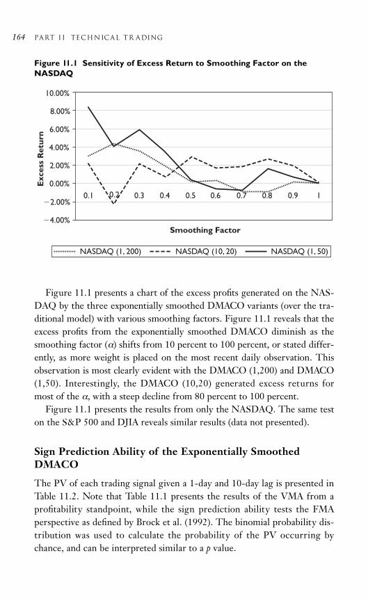
Figure 11.1 presents a chart of the excess profits generated on the NAS-DAQ by the three exponentially smoothed DMACO variants (over the tra-ditional model) with various smoothing factors. Figure 11.1 reveals that theexcess profits from the exponentially smoothed DMACO diminish as thesmoothing factor (α) shifts from 10 percent to 100 percent, or stated differ-ently, as more weight is placed on the most recent daily observation. Thisobservation is most clearly evident with the DMACO (1,200) and DMACO(1,50). Interestingly, the DMACO (10,20) generated excess returns formost of the α, with a steep decline from 80 percent to 100 percent.
Figure 11.1 presents the results from only the NASDAQ. The same teston the S&P 500 and DJIA reveals similar results (data not presented).
Sign Prediction Ability of the Exponentially SmoothedDMACO
The PV of each trading signal given a 1-day and 10-day lag is presented inTable 11.2. Note that Table 11.1 presents the results of the VMA from aprofitability standpoint, while the sign prediction ability tests the FMAperspective as defined by Brock et al. (1992). The binomial probability dis-tribution was used to calculate the probability of the PV occurring bychance, and can be interpreted similar to a p value.
164 Part I i TECHNICAL TR ADING
10.00%
8.00%
6.00%
4.00%
Exc
ess
Ret
urn
2.00%
0.00%
Smoothing Factor
0.1 0.2 0.3 0.4 0.5 0.6 0.7 0.8 0.9 1
NASDAQ (1, 200) NASDAQ (10, 20) NASDAQ (1, 50)
2.00%
4.00%
Figure 11.1 Sensitivity of Excess Return to Smoothing Factor on theNASDAQ

chapter 11 Profiting from the Dual-Moving Average 165
Table 11.2 Predictive Value (PV) of Buy and Sell Signals
Panel A. Lag 1
DMACO DMACOTraditional Calculation Exponentially Smoothed
STMA,LTMA STMA,LTMA
Market Index 1,50 10,50 1,200 1,50 10,50 1,200
S&P 500 (N 2,596)
Buy Signal, PV 56.7% 40.0% 48.8% 61.9% 33.3% 62.5%
BPD Probability 0.03 0.82 0.71 0.19 0.95 0.19
Sell Signal, PV 38.9% 0.0% 34.9% 42.9% 52.4% 50.0%
BPD Probability 0.99 NA 0.99 0.80 0.50 0.50
Dow Jones (N 2,596)
Buy Signal, PV 48.5% 60.0% 54.1% 50.0% 54.5% 50.0%
BPD Probability 0.69 0.37 0.26 0.50 0.41 0.50
Sell Signal, PV 49.5% 60.0% 50.8% 45.8% 59.1% 46.2%
BPD Probability 0.70 0.37 0.53 0.73 0.42 0.50
NASDAQ (N 2,596)
Buy Signal, PV 47.5% 22.2% 55.3% 52.6% 63.2% 62.5%
BPD Probability 0.81 0.99 0.21 0.50 0.17 0.17
Sell Signal, PV 48.8% 44.4% 47.4% 42.1% 52.6% 44.4%
BPD Probability 0.83 0.98 0.71 0.67 0.49 0.69
Panel B. Lag 10
DMACO DMACOTraditional Calculation Exponentially Smoothed
STMA,LTMA STMA,LTMA
Market Index 1,50 10,50 1,200 1,50 10,50 1,200
S&P 500 (N 2,596)
Buy Signal, PV 55.6% 60.0% 58.1% 57.1% 61.9% 87.5%
BPD Probability 0.17 0.19 0.18 0.33 0.19 0.03
Sell Signal, PV 43.3% 40.0% 23.2% 52.4% 61.9% 12.5%
BPD Probability 0.91 0.93 0.99 0.50 0.19 0.99
Dow Jones (N 2,596)
Buy Signal, PV 53.5% 80.0% 44.3% 54.2% 63.6% 50.0%
BPD Probability 0.27 0.03 0.84 0.42 0.14 0.50
Sell Signal, PV 44.4% 20.0% 62.3% 54.2% 45.% 53.8%
BPD Probability 0.88 0.95 0.03 0.42 0.73 0.5
NASDAQ (N 2,596)
Buy Signal, PV 57.5% 55.6% 55.3% 63.2% 68.4% 75.0%
BPD Probability 0.11 0.20 0.42 0.17 0.08 0.05
Sell Signal, PV 37.5% 55.6% 50.0% 63.2% 47.4% 55.6%
BPD Probability 0.99 0.20 0.50 0.17 0.67 0.33
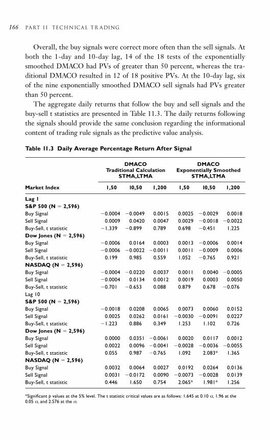
Overall, the buy signals were correct more often than the sell signals. Atboth the 1-day and 10-day lag, 14 of the 18 tests of the exponentiallysmoothed DMACO had PVs of greater than 50 percent, whereas the tra-ditional DMACO resulted in 12 of 18 positive PVs. At the 10-day lag, sixof the nine exponentially smoothed DMACO sell signals had PVs greaterthan 50 percent.
The aggregate daily returns that follow the buy and sell signals and thebuy-sell t statistics are presented in Table 11.3. The daily returns followingthe signals should provide the same conclusion regarding the informationalcontent of trading rule signals as the predictive value analysis.
166 Part I i TECHNICAL TR ADING
Table 11.3 Daily Average Percentage Return After Signal
DMACO DMACOTraditional Calculation Exponentially Smoothed
STMA,LTMA STMA,LTMA
Market Index 1,50 10,50 1,200 1,50 10,50 1,200
Lag 1S&P 500 (N 2,596)Buy Signal 0.0004 0.0049 0.0015 0.0025 0.0029 0.0018Sell Signal 0.0009 0.0420 0.0047 0.0029 0.0018 0.0022Buy-Sell, t statistic 1.339 0.899 0.789 0.698 0.451 1.225Dow Jones (N 2,596)Buy Signal 0.0006 0.0164 0.0003 0.0013 0.0006 0.0014Sell Signal 0.0006 0.0022 0.0011 0.0011 0.0009 0.0006Buy-Sell, t statistic 0.199 0.985 0.559 1.052 0.765 0.921NASDAQ (N 2,596)Buy Signal 0.0004 0.0220 0.0037 0.0011 0.0040 0.0005Sell Signal 0.0004 0.0134 0.0012 0.0019 0.0003 0.0050Buy-Sell, t statistic 0.701 0.653 0.088 0.879 0.678 0.076Lag 10S&P 500 (N 2,596)Buy Signal 0.0018 0.0208 0.0065 0.0073 0.0060 0.0152Sell Signal 0.0025 0.0262 0.0161 0.0030 0.0091 0.0227Buy-Sell, t statistic 1.223 0.886 0.349 1.253 1.102 0.726Dow Jones (N 2,596)Buy Signal 0.0000 0.0351 0.0061 0.0020 0.0117 0.0012Sell Signal 0.0022 0.0096 0.0041 0.0028 0.0036 0.0055Buy-Sell, t statistic 0.055 0.987 0.765 1.092 2.083* 1.365NASDAQ (N 2,596)Buy Signal 0.0032 0.0064 0.0027 0.0192 0.0264 0.0136Sell Signal 0.0031 0.0172 0.0090 0.0073 0.0028 0.0139Buy-Sell, t statistic 0.446 1.650 0.754 2.065* 1.981* 1.256
*Significant p values at the 5% level. The t statistic critical values are as follows: 1.645 at 0.10 α, 1.96 at the0.05 α, and 2.576 at the α.

The return analysis is consistent with the profitability and predictivevalue tests. At the 1-day lag, the returns following a buy signal were posi-tive in four of nine for the traditional DMACO, while the exponentiallysmoothed DMACO buy signals were followed by positive returns in six ofthe nine tests. At the 10-day lag, all nine tests of the exponentiallysmoothed DMACO’s buy signal generated positive returns. The sell signalsdo not appear to be as predictive. At the 1-day lag, negative returns follow-ing a sell signal in four of nine for the traditional DMACO, while the expo-nentially smoothed DMACO’s sell signals were followed by negativereturns in only three of the nine tests. However, at the 10-day lag, theexponentially smoothed DMACO’s sell signal was followed by negativereturns in seven of the nine tests. These results are similar to prior studies(Brock et al.,1992; Lento & Gradojevic, 2007).
The results from the sign prediction tests (predictive value and returnanalysis) are consistent with the profitability tests, and corroborate theproposition that the exponentially smoothed DMACO results in fewer,more powerful signals than the traditional DMACO model.
CONCLUSION
This chapter provides new insights into the profitability of technical analy-sis by developing and testing a trading model that is shown to earn abnor-mal profits, and predict future price movements. The exponentiallysmoothed DMACO was tested on the S&P 500, NASDAQ, and DJIA forthe period January 1999 to April 2009. The results suggest that the prof-itability of DMACO is significantly enhanced when the STMA and LTMAare calculated with the exponential smoothing technique. The increasedprofitability is significant, in many cases in excess of 5.0 percent per annum,and consistent across each moving average combination and data set.
The additional profits are not the result of increased risk. Rather, expo-nentially smoothing prices results in a fewer number of signals that aremore informative. The results from the sign prediction tests are consistentwith the profitability tests as large, positive returns follow the buy signal ofthe exponentially smoothed DMACO.
This study also investigated the sensitivity of the profits to the smooth-ing factor, and reveals that the profits decline as the smoothing factorincreases (i.e., as more weight is placed on the most recent observation).Researchers are encouraged to further explore the profitability of the
chapter 11 Profiting from the Dual-Moving Average 167

DMACO by utilizing different smoothing technique. For example, theSTMA and LTMA can be calculated on a time-series that has beensmoothed with a double or triple exponential smoothing technique asopposed to the single exponential smoothing technique.
The traditional DMACO trading rules have been shown to be profitableas inputs into the combined signal approach (Lento, 2008). Investors canalso explore the profitability of the exponentially smoothed DMACO byjointly employing the individual DMACO trading rules into the combinedsignal approach (Lento, 2008; Lento, 2009).
REFERENCES
Bessembinder, H. and Chan, K. (1998) Market efficiency and the returns totechnical analysis. Financial Management, 27(2): 5–17.
Brock, W., Lakonishok, J., and LeBaron, B. (1992) Simple Technical Trad-ing Rules and the Stochastic Properties of Stock Returns. Journal ofFinance, 47(5): 1731–1764.
Gençay, R. (1998) The Predictability of Security Returns with SimpleTechnical Trading Rules. Journal of Empirical Finance, 5(4): 347–359
Gençay, R. (1999) Linear, Non-Linear and Essential Foreign ExchangeRate Prediction with Simple Technical Trading Rules. Journal of Inter-national Economics, 47: 91–107.
Gençay, R. and Stengos, T. (1998) Moving Average Rules, Volume and thePredictability of Security Returns with Feedforward Networks. Jour-nal of Forecasting, 17(5–6): 401–414.
Hyndman, R.J., Koelher, A.B., Ord, J.K., and Snyder, R.D. (2008) Fore-casting with Exponential Smoothing. Springer Series in Statistics. Berlin:Springer-Verlag.
Kho, B.C. (1996) Time-Varying Risk Premia, Volatility, and TechnicalTrading Profits: Evidence from Foreign Currency Futures Markets.Journal of Financial Economics, 41( June 1996): 249–290.
Lento, C. (2007) Test of Technical Analysis in the Asian-Pacific EquityMarkets: A Bootstrap Approach. Academy of Accounting and FinancialStudies Journal, 11(2): 51–74.
Lento, C. (2008) A Combined Signal Approach to Technical Analysis onthe S&P 500. Journal of Business & Economics Research, 6(8): 41–51.
168 Part I i TECHNICAL TR ADING

Lento, C. (2009) Combined Signal Approach: Further Evidence from theAsian-Pacif ic Equit y Markets. Applied Economics Let ters, 16(7):749–753.
Lento, C. and Gradojevic, N. (2007) The Profitability of Technical TradingRules: A Combined Signal Approach. Journal of Applied BusinessResearch, 23(1): 13–28.
Levich, R. and L. Thomas. (1993) The Significance of Technical TradingRules Profits in the Foreign Exchange Market: A Bootstrap Approach.Journal of International Money and Finance, 12(5): 451–474.
Levich, R.M. (2001) The Importance of Emerging Capital Markets. Publishedin R. Litan and R. Herring (eds.), Brookings-Wharton Papers on FinancialServices, Washington, D.C.: The Brookings Institution, pp. 1–45
Lo, A.W., Mamaysky, H., and Wang, J. (2000) Foundations of TechnicalAnalysis: Computational Algorithms, Statistical Inference, and Empiri-cal Implementation. Journal of Finance, 55(4): 1705–1765.
Lui, Y.H. and D. Mole. (1998) The Use of Fundamental and TechnicalAnalyses by Foreign Exchange Dealers: Hong Kong Evidence. Journalof International Money and Finance, 17(3): 535–545.
Murphy, J. (2000) Charting Made Easy. Glenelg, MD: Marketplace Books.
Neely, C., Weller, P., and Dittmar, R. (1997) Is Technical Analysis in the Foreign Exchange Market Profitable? A Genetic Programming Approach.Journal of Financial and Quantitative Analysis, 32 (December): 405–426.
Neftci, S. (1991) Naive Trading Rules in Financial Markets andWiener–Kolmogorov Prediction Theory: A Study of Technical Analy-sis. Journal of Business, 64(4): 549–571.
Pring, M.J. (2002) Technical Analysis Explained. New York: McGraw-Hill.
Satterthwaite, F.E. (1946) An Approximate Distribution of Estimates ofVariance Components. Biometrics Bulletin, 2: 110–114.
Taylor, M.P. and Allen, H. (1992) The Use of Technical Analysis in theForeign Exchange Market. Journal of International Money and Finance,11(3): 304–314.
White, H. (2005) Approximate Nonlinear Forecasting Methods. In: Elliot,G., Gragner, C.W.J., and Timmerman, A. (eds.), Handbook of EconomicsForecasting. Amsterdam: North-Holland Elsevier.
chapter 11 Profiting from the Dual-Moving Average 169

NOTES
1. This section is not intended to be a comprehensive review of the litera-ture on moving average trading rules. Readers interested in a literaturereview are encouraged to read Pring (2002).
2. Note that this test statistic does not always conform to the student dis-tribution. However, an approximation for the degrees of freedom wasdeveloped by Satterthwaite (1946). If the number of observations issufficiently large, this test statistic will converge to a standard normaldistribution and the t-table critical values can be used.
170 Part I i TECHNICAL TR ADING

171
12C H A P T E R
ShareholderDemands and theDelaware DerivativeAction
Edward Pekarek
ABSTRACT
Among the most “interesting and ingenious” corporate “accountabilitymechanisms” is the shareholder derivative action. An aggrieved investormay demand the independent directors of a corporate issuer to litigate onbehalf of the corporation, for harm(s) allegedly committed upon the corpo-ration. This chapter explores who is eligible to sue derivatively and identi-fies some of the basic requirements to initiate derivative litigation.
INTRODUCTION
The efficient market hypothesis (EMH) presumes that existing stock pricesalways reflect the entire universe of information that is relevant to a givensecurity. The EMH posits that the so-called “free” market functions as apure pricing mechanism and equities will always trade at their relative “fairvalue” in a liquid and transparent market, leaving investors facing theimpossible, at least in theory, to outperform the overall market throughexpert portfolio strategies, stock selection or market timing.
Various studies, including a number of those analyzed in the precedingchapters of this section, have revealed the possibility that technical trading

rules may produce investment results which are superior to traditional“buy and hold” portfolio selection strategies. While the application oftechnical trading rules may result in an increased probability of investmentsuccess, no amount of portfolio selection modeling, no matter how pre-scient, can prevent, or predict precisely, the presence of concealed corpo-rate wrongdoing.
While some trading models utilize historical data such as moving aver-ages, and still others seek to extrapolate future results through the use ofnonlinearity-enhanced technical models or pattern recognition techniques,corporate insiders can, and do, go to great lengths to prevent transgressionssuch as self-dealing from being discovered by the market. Of course, oneneed only look to the headlines in the financial media during the macrodecline of 2008 and 2009 for ample evidence that corporate wrongdoing isjust as prevalent today as it was during the cynical era of Enron, or the“wild west” environment which made Jesse Livermore infamous.
This necessarily begs the question of how statistical modeling has consis-tently failed to detect this sort of undisclosed insider activity, and if theEMH pricing mechanism does properly discount all relevant information atany given moment, insider misconduct such as that which occurred in theEnron, Tyco, Worldcom, HealthSouth, or Adelphia scandals, should simplynever have the chance to fester into enterprise-destroying frauds withoutbeing discovered. Nonetheless, sage fund managers, such as James Chanos,profit from a fraud scheme’s imminent collapse through short-sale strate-gies. See Chanos (2002).
Some pundits maintain technical analysis and trading acumen can beconfounded by market manipulation. See Degraaf (2009). Still others viewchart interpretation and analysis as something akin to a “methodology forinterpreting . . . the behavior of [humans] and markets” through a recordof “inerasable fingerprints of human nature made graphic in the greateststruggle, next to war, in human experience” Edwards, Magee, and Bassetti(2007). The question of whether technical analysis can reveal such manip-ulation, as well as other forms of wrongdoing involving the managers ofpublicly held issuers, the corporate board of directors, is not the topic ofthis chapter. See 8 Del. C. § 141. This chapter contemplates some of theremedies available to shareholders of Delaware corporations where suchwrongdoing has occurred.
Among the more “interesting and ingenious” corporate “accountabilitymechanisms” devised by common law to address such wrongdoing, is the
172 Part i I TECHNICAL TR ADING

shareholder derivative action. Kramer, 546 A.2d at 351; see also Block, Bar-ton, and Radin (1987). Derivative litigation has been instituted by share-holders of Delaware corporations in federal courts throughout the UnitedStates. See In re CNET Networks, Inc., 483 F. Supp. 2d 947; In re Bristol-Myers Squibb, 2007 WL 959081; Prince, 148 Fed. Appx. 249. The necessaryinitial step a shareholder must take in pursuit of derivative relief is to com-municate a demand to the corporation’s “independent” directors, in which itmust articulate the specific relief she or he seeks. If the “independent”director(s) refuse to take the action(s) demanded by the shareholder, or, if alawful basis exists for the shareholder to be excused from the demandrequirement, derivative litigation may proceed, provided certain otherrequirements are first satisfied.
Unlike claims for breach of duty, securities fraud, and the like, where theplaintiff(s) typically seeks relief related to alleged harms committed uponthem as individuals by corporate fiduciaries, and perhaps by others, deriva-tive litigation is reportedly “popular” because stock losses are not requiredto bring an action, as is the case with securities fraud litigation (Koppel,2009). A typical shareholder derivative action involves the pursuit of civiland/or equitable relief on behalf of a corporation in which an investor ownsan equity stake, often in the form of common stock. Blasband, 971 F.2d at1040. The derivative shareholder litigates as a nominal plaintiff only, actingon behalf of the corporation in which she or he owns equity, for harm(s)allegedly committed upon the corporation, and as the term suggests, one whosues derivatively, “seeks redress on behalf of the corporation.” Kramer, 546A.2d at 351; see also Block, Barton, and Radin (1987); Ryan, 918 A.2d at349. Pre-suit requirements established by Delaware law contain subtlenuances, some of which can result in the dismissal of a derivative action ifperformed improperly or ignored.
POLICY PURPOSES FOR DERIVATIVE ACTIONS
Delaware law developed the derivative action as a mechanism to enforce var-ious rights of the corporation, and indirectly, its stakeholders, through theassertion of civil (and/or equitable) claims on behalf of that corporation,which, it has itself refused, Kramer, 546 A.2d at 351; see also Block, Barton,and Radin (1987), or “failed to enforce [rights] which may properly beasserted.” Aronson, 473 A.2d at 808 n.1; Maldonado, 413 A.2d at 1255; Harff,324 A.2d at 218; Cantor, 18 Del. Ch. 359. A shareholder suing derivatively is
chapter 12 the Delaware Derivative Action 173

a nominal litigant, acting on behalf of and for the benefit of the corporation,which is named, nominally, as a defendant that is concurrently the indispen-sable, Agostino, 845 A.2d at 1116–17 n.15, “real party in interest to whichany recovery usually belongs.” Schuster, 127 Cal. App. 4th at 312; see also In re Tyson Foods, Inc., 919 A.2d 563; Maldonado, 413 A.2d at 1255; Levine,219 A.2d at 145; Slutzker, 28 A.2d at 528; Solimine, 19 A.2d at 344. Corpo-rate policy reforms and relief of other ilk may result from a successful deriv-ative action, but the shareholder(s) recover(s) no money damages. At leastone court has recently treated the shareholder of a corporation as a fiduciaryfor the purposes of derivative litigation. Egelhof, 2008 WL 352668. Direc-tors and the nominal defendant corporation typically retain separate counsel due to the inherent tension unique to derivative litigation. Kolbe, 1988 WL 110511, at *1.
A nominal corporate defendant’s state of incorporation is generally thesource of the substantive (and certain procedural) law applied, including thespecific derivative demand requirements, compare Fed. R. Civ. P. R. 23.1with Del. Ch. R. 23.1, as well as any related demand(s) for books andrecords. See 8 Del. C. § 220. According to New York law, “issues related tothe ‘internal affairs’ of a corporation are decided under the law of the stateof incorporation because that state has an interest superior to that of otherstates in regulating the internal affairs of its corporation.” Potter, 11 Misc.3d at 965–66. Notwithstanding the above, a shareholder’s first obstacle isoften navigating the demand requirements of Delaware law, because of itsinfluence as the “preeminent . . . place for businesses to incorporate sincethe early 1900s,” and accordingly, due to the significant number of publiclyheld concerns which are Delaware corporations (Black, 2007).
DEMAND REQUIREMENTS
Because derivative litigation “impinges on the managerial freedom ofdirectors,” a shareholder can only initiate a derivative suit subsequent tothe assertion of a written demand upon the independent directors thatarticulated actions be pursued on behalf of the corporation. Stone, 911A.2d at 366. Both the Federal Rules of Civil Procedure and the DelawareChancery Court Rules, with limited exceptions, require that a demand bemade and served upon a corporation’s directors. Compare Del. Ch. CourtR. 23.1 with Fed. R. Civ. P. 23.1. Rule 23.1 of the Federal Rules of CivilProcedure codif ied a long-standing common law requirement that a
174 Part i I TECHNICAL TR ADING

shareholder must first make a demand upon directors before initiatingderivative litigation. See Fed. R. Civ. P. 23.1; Mullins, 45 F.Supp. 871;Findley, 240 P.2d 421. In a so-called “double” derivative suit, in which ashareholder of a parent corporation alleges injury(ies) to a subsidiary, anydemand(s) must also be made on the subsidiary directors, unless thedemand is excused by law, for example, by what is known as “futility,” afactual condition which must first be demonstrated as to the directors ofboth the subsidiary and the parent. Rales, 634 A.2d at 934.
A shareholder demand should “alert the [b]oard of [d]irectors so that itcan take such corrective action, if any, as it feels is merited.” Allison, 604F.Supp. at 1117. The derivative demand is also a mechanism designed “tocurb a myriad of individual shareholders from bringing potentially frivo-lous lawsuits on behalf of the corporation, which may tie up the corpora-tion’s governors in constant litigation and diminish the board’s authorityto govern the affairs of the corporation.” Ryan, 918 A.2d at 352; see alsoFed. R. Civ. P. 23.1; Del Ch. Court R. 23.1. One district court recentlycriticized “scandalous” derivative litigation, and opined that it typified“[t]he very abuses that led to the reform embodied by the PSLRA perme-ate the world of derivative litigation.” In re JPMorgan Chase & Co., 2008WL 4298588, at *10; id.
Delaware and federal rules offer little guidance regarding what mustactually appear within a shareholder demand. Neither rule provides specificdetail as to other mechanical and procedural aspects of a proper demand.Rule 23.1 does clearly mandate, however, that a valid shareholder demandmust be made upon directors of the corporation, or upon a “comparableauthority.” If such a demand is not communicated to the corporation’sdirectors, the shareholder’s pleadings must articulate in detail the reason(s)for failure to assert a demand. See Simon, 775 N.Y.S.2d at 317; id. Delawarecourts have detailed technical requirements for shareholder demands. SeeAllison, 604 F.Supp. at 1117; id.
All “Reasonably Available” Information Should Be Gatheredfor a Demand
A prudent shareholder will expend all reasonable efforts and exhaust allreasonable means to gather relevant facts prior to bringing derivative liti-gation, and the due diligence performed prior to crafting a demand shouldbe no exception. Beam I, 845 A.2d at 1056; id. Potential sources of relevant
chapter 12 the Delaware Derivative Action 175

information for an investigating shareholder include: SEC filings, local tax authority records, county property records, state and federal courtdockets, secretaries of state corporation filings; as well as a variety of non-government sources, including media reports, press releases, investor rela-tions representatives, corporate Web sites and business data sources such asBloomberg, Dun & Bradstreet, Hoovers, Westlaw, and Lexis; and self-reg-ulatory organizations such as stock exchanges and the Financial IndustryRegulatory Authority (“FINRA”). Rales, 634 A.2d at 935 n.10.
Shareholders contemplating derivative litigation are encouraged by courtsto employ Delaware’s Section 220 demand to inspect corporate books andrecords as a fact-finding tool prior to initiating a derivative action. See, e.g.,id. If a tribunal determines that a failure to employ a Section 220 demandbefore initiating derivative litigation was unreasonable, under the circum-stances of the case, the risk of dismissal is substantial. Id. If a shareholderseeks to be excused from the demand requirement, it is virtually expectedthat the shareholder will have first “used a Section 220 books and recordsinspection to uncover such facts,” before seeking relief from the DelawareChancery Court. Id.; Beam II, 833 A.2d at 983–84; see In re Walt Disney Co.,825 A.2d at 279; see also Beam I, 845 A.2d at 1056 n.51.
Many legitimate uses exist for the information that results from corpo-rate books and records inspections, such as “bring[ing] a derivative suit inthe case of corporate waste or mismanagement, or to bring a suit attachingsome aspect of a company’s public disclosures,” or to evaluate the proprietyof the refusal by directors to satisfy the terms of a shareholder demand. See,e.g., Disney, 2005 WL 1538336, at *5; see also Grimes, 724 A.2d at 564. A Delaware court recently noted that directors are afforded an opportunityto “exculpate themselves” in the face of a Section 220 demand. In re TysonFoods, Inc., 919 A.2d at 578.
The Section 220 inspection provisions function, inter alia, to: (i) investi-gate a company’s suspected wrongdoing; (ii) ensure that it can prepare athorough shareholder demand; and (iii) form the basis of a particularizedpleading; and (iv) “can serve as a ‘tool at hand’ [for directors] to defendagainst unfounded charges of wrongdoing.” Id. at 578 n.20. The uniqueopportunity for directors to inform aggrieved shareholders, and to demon-strate the directors exercised good faith business judgment in the disputedmanagerial decisions, including responses to shareholder demands, serves asa valuable by-product of the requirement that a shareholder must conduct aduly diligent investigation of all reasonably available information prior to
176 Part i I TECHNICAL TR ADING

asserting a demand. The liberal use of Section 220 inspections before filinga derivative action supports the ideal of judicial economy pragmatically,because it may deter some meritless litigation. Id.
At least one Delaware jurist has noted, with apparent disappointment,“surprisingly, little use has been made of section 220,” he speculated thebooks and records demand remains fallow, in the derivative context, due to“an unseemly race to the court house, chiefly generated by the ‘first to file’custom seemingly permitting the winner of the race to be named leadcounsel.” Rales, 634 A.2d at 935 n.10. Considering the depth of factualdetail often required to assert a shareholder demand properly, and mindfulof the Delaware courts’ criticism of litigants who have not utilized the toolsmade available to them, a Section 220 demand to inspect corporate booksand records is likely part of a prudent course of conduct prior to the asser-tion of a derivative demand upon a corporation’s independent directors.
Demand Deadlines: When Must Directors Respond?
Delaware law affords directors broad discretion to determine whether tobring a lawsuit on behalf of the corporation they manage in response to ashareholder demand. 8 Del. C. § 141(a); see also In re IAC/InterActiveCorp.Sec. Litig., 478 F. Supp. 2d. at 598. Directors of Delaware corporations aregenerally protected from liability for refusing a shareholder demand, pro-vided the decision was not “wrongful,” meaning that the refusal was: (i) a legitimate exercise of the directors’ good faith business judgment; and(ii) a sound exercise of lawful discretion. Aronson, 473 A.2d at 813; id. Theamount of time directors are permitted to render decisions regarding share-holder demands varies widely, with “no precise rule as to how much time a[b]oard must be given to respond to a demand.” Allison, 604 F.Supp. at1117–18. Procedural rules do not specify how long recipient directors haveto respond to a shareholder demand.
Delaware courts consider complexities of contended issues and thedirectors’ actions in response to a proper shareholder demand. Wheredirectors do not respond to a shareholder demand, jurists employ fact-intensive analysis, guided by a rule of reason, in order to determinewhether the time between the assertion of a shareholder demand, and thefiling of a derivative action, is appropriate or premature. One such courtheld a derivative suit initiated one month after asserting a shareholderdemand was appropriate, Rubin, 701 F. Supp. at 1046, while another found
chapter 12 the Delaware Derivative Action 177

the filing of a derivative complaint roughly 10 weeks after serving ademand was premature, reasoning the “magnitude and complexity” ofcontested issues warranted affording the directors additional time todecide, see Allison, 604 F.Supp. at 1118, while yet another tribunal found aneight-month interval to be insufficient, due to the particular complexitiesof that case. Mozes, 638 F. Supp. at 221.
Juridical determination of whether the initiation of derivative litigationis premature is guided by a case-by-case consideration which utilizeshighly fact-intensive f indings to scrutinize whether directors haveinformed themselves “of all material information essential to an objectiveand meaningful evaluation of the demand.” Allison, 604 F.Supp. at1117–18; Abramowitz, 513 F.Supp. at 132–33. This standard suggests thedegree of detail provided by a shareholder derivative demand mightdirectly influence what is perceived to be a reasonable amount of time fordirectors to respond. Perhaps an inversely correlative relationship existsbetween: (i) the amount of time directors are afforded to render a decisionregarding a shareholder demand; and (ii) the depth of detail within thefactual information provided in such a demand, relative to the factualcomplexity of the disputed issue(s).
STANDING TO SUE DERIVATIVELY
A timely, duly diligent, and otherwise proper demand that directors initiatesuit on behalf of the corporation is a condition precedent to the commence-ment of Delaware derivative litigation. Del. Ch. Court R. 23.1; Fed. R. Civ.P. 23; see also In re eBay, Inc. Shareholders Litig., 2004 WL 253521, at *2; seealso In re J.P. Morgan Chase & Co., 2005 WL 1076069, at *8. Absent a legalexcuse, it is a “threshold question of standing as to whether the shareholderhas made a demand on the board of directors.” In re IAC/InterActiveCorpSec. Litig., 478 F. Supp. 2d at 597. The viability of a derivative suit can turnon the initial inquiry of whether the shareholder has competently pleadedstanding relative to an allegedly wrongful refusal of a properly asserteddemand, or of the futility of asserting such a demand, which, if established,would obviate the demand requirement. Miller, 1992 WL 329313, at *5; seealso Futility discussion, infra. A shareholder who contends she or he hasstanding to sue derivatively, as a function of legal excuse due to demandfutility, must adhere to alternative pleading requirements set forth in Dela-ware Chancery Rule 23.1. Id.; see also id. at *5 n.10.
178 Part i I TECHNICAL TR ADING
Continued Shareholder Status
In order to impose a derivative demand upon a Delaware corporation, aprospective nominal plaintiff “must have been a shareholder at the time ofthe challenged transaction[s] to have standing to maintain a shareholderderivative suit.” Blasband, 971 F.2d at 1040. That putative plaintiff musthave been a genuine stakeholder in the corporation, concurrent with anyalleged wrongdoing, and she or he must retain shareholder status through-out the course of derivative litigation. See id. at 1041; Lewis, 477 A.2d at1046; see also 8 Del. C. § 327.
The “sole purpose” of this continuing ownership requirement is to pre-vent the “evil” of opportunistic plaintiffs from purchasing stock in a Dela-ware corporation simply “in order to maintain a derivative action designedto attack a transaction which occurred prior to the purchase of the stock.”Id. at 1040–41. The requirement that a derivative plaintiff retains share-holder status throughout the case “ensures that the plaintiff has sufficientincentive to represent adequately the corporation’s interests during litiga-tion.” Id. at 1041. The presumptive legislative intent of these statutory pro-visions is to prevent abuse of the derivative action mechanism. Id. Delawarelaw apparently does not, however, require the plaintiff to hold the entireposition in the stock of the corporation being sued derivatively throughoutthe pendency of such litigation. This may be especially relevant where ashareholder also contemplates a separate action for securities fraud andmight face somewhat competing issues, such as those which involve losscausation. See, e.g., Dura Pharmaceuticals, 544 U.S. 336.
FUTILITY EXCUSES THE DEMANDREQUIREMENT
If a shareholder demand asserted on a corporation’s directors would bepointless, or “futile,” the requirement of a demand letter is excused as amatter of law, and a derivative action may proceed, provided futility is“well-pleaded.” See Fed. R. Civ. P. 23.1; see also In re IAC/InterActive CorpSec. Litig., 478 F. Supp. 2d at 598. The primary purpose of the demandrequirement is to afford directors the “opportunity to examine the allegedgrievance and related facts and to determine whether pursuing the action isin the best interest of the corporation.” Ryan, 918 A.2d at 352 n.20; see alsoFed. R. Civ. P. 23.1; Del. Ch. Ct. R. 23.1. However, directors might not
chapter 12 the Delaware Derivative Action 179

always be inclined to act in the best interest of a corporation in which aputative shareholder-plaintiff holds a stake. One such example where ashareholder might be excused due to demand futility is where “directors areincapable of making an impartial decision regarding whether to institutesuch litigation.” Stone, 911 A.2d at 366. Delaware courts have recognizedwhere “a question is rightfully raised over whether the board will pursuethese claims with 100% allegiance to the corporation, since doing so mayrequire that the board sue itself on behalf of the corporation,” a demandmay be excused due to futility. Ryan, 918 A.2d at 354.
FUTILITY, DIRECTOR INDEPENDENCE, ANDBUSINESS JUDGMENT
The director of a Delaware corporation is presumed to be incapable ofacting objectively in the context of a shareholder demand if she or he is“interested in the outcome of the litigation.” Grimes, 673 A.2d 1207; see also In re eBay, Inc., 2004 WL 253521. Delaware courts consider a“classic example[ ]” of director self-interest to be “a business transactioninvolv[ing] either a director appearing on both sides of a transaction or [ ]receiving a [ ] benefit from a transaction not received by the shareholdersgenerally.” Berger, 2005 WL 2807415, at *6. Delaware law provides atleast “two instances where a plaintiff is excused from making demand.”Ryan, 918 A.2d at 352. A shareholder can first raise reasons that cast doubtregarding the independence, or disinterest, of a majority of the corpora-tion’s directors. Id.; Zimmerman, 2002 WL 31926608, at *7. For example,where “three directors of a six person board are not independent andthree directors are independent, there is not a majority of independentdirectors and demand would be futile.” Beam I, 845 A.2d at 1046 n.8; cf.In re Oracle Corp., 824 A.2d 917.
A second manner in which a shareholder may be excused from therequired demand is to plead particularized reasons which raise reasonabledoubts that the corporate acts connected to the alleged wrongdoing werenot a product of the board’s valid exercise of business judgment. Ryan, 918A.2d at 352; see also Del. Ch. Ct. R. 23.1. Courts generally respect the deci-sions made by corporate directors, unless a shareholder alleges a majority ofthe directors lacked independence in relation to a contested decision, orthat certain directors are actually interested in the transaction(s) at issue,and did “not act in good faith, act[ed] in a manner that cannot be attributed
180 Part i I TECHNICAL TR ADING

to a rational business purpose, or reach[ed] their decision by a grossly neg-ligent process that include[d] the failure to consider all material facts rea-sonably available.” Berger, 2005 WL 2807415, at *6.
A recent Delaware decision found a shareholder established demandfutility with pleading allegations that detailed wrongdoing committed by acompensation committee of the nominal defendant corporation’s board ofdirectors, and where members of that compensation committee also consti-tuted the board’s majority; the shareholder also raised sufficient doubtschallenging whether the disputed transactions were actually the result of avalid exercise of business judgment. Ryan, 918 A.2d at 354. Similarly, ifa board’s majority includes familial or material financial interest(s); or if thedirectors are for some other reason unable to act independently, such ascontrol or domination; or if it is otherwise established the “underlyingtransaction is not the product of a valid exercise of business judgment,” theputative plaintiff would be excused from the required pre-suit derivativedemand. Beam I, 845 A.2d at 1049.
A director is considered to be “interested,” in the derivative context, if itcan be demonstrated that she or he will incur a potential personal benefit,or avoid a detriment, that is not equally shared by the stockholder(s), as aresult of the outcome of a decision detailed in the derivative demand. Id.Whether a director can exercise independent and good faith business judg-ment is often answered by analyzing the “personal consequences resultingfrom the decision.” Id. The “primary basis” for measurement of the extent(or lack) of a director’s independence is “whether the director’s decision isbased on the corporate merits of the subject before the board, rather thanextraneous considerations or influences.” Id. When a shareholder can showthat the majority of a board’s directors lack independence, no demand isrequired and the shareholder may proceed with the litigation derivatively.
CONCLUSION
The corporate accountability mechanism of a Delaware derivative actionrequires a shareholder to thoroughly investigate the facts related to allegedwrongdoing and be duly diligent in obtaining all reasonably available infor-mation, utilizing various government and non-government sources, as wellas a Section 220 corporate books and records inspection demand. A Dela-ware corporation’s directors must discharge the duty to be fully informedwhen making the decision of whether to refuse a shareholder demand, or to
chapter 12 the Delaware Derivative Action 181

initiate an action on behalf of the corporation, and must make that decisionas a good faith exercise of valid business judgment in order to withstandsubsequent challenges by the shareholder. A demand must be asserted forwhat has been described as a “proper purpose.”
Directors who are “interested,” or who cannot be considered “independ-ent,” need not be served with a shareholder demand, and if the majority of aDelaware corporation’s board of directors cannot be construed as disinter-ested or independent, a shareholder can proceed directly to litigation, withreliance on the doctrine of futility, excused of the condition precedent toserve a derivative demand. However, judicial evaluations have differed greatlyregarding the question of the disinterest and/or independence of directors.
A shareholder must carry the burden of establishing reasonable doubt asto director interest or dependence when seeking to be excused from thedemand requirement. A shareholder might be able to reduce the time that isreasonable for a board to decide whether to accept or refuse a demand byproviding as much relevant factual detail as is reasonably possible about thecontested transactions and/or activities. Delaware courts undertake exactingreviews of the factual complexities of a shareholder demand in order todetermine whether an action was initiated prematurely, and the outcome ofthose evaluations can vary greatly, but the analysis is typically governed bya rule of reason. The overall rigor required of shareholders also extends tothe degree of particularity that is expected of a derivative pleading, whichsupports a policy of judicial economy by preventing meritless lawsuits thatmight otherwise encumber the limited managerial resources of Delawarecorporations, to the potential detriment of its other shareholders.
The derivative action truly is an ingenious corporate accountabilitymechanism. When a shareholder discovers facts that indicate potential harmhas been brought upon the corporate form, it is unlike any other legal meas-ure designed to empower shareholders. However, the many nuances of deriv-ative litigation, and its particular pre-litigation requirements, are sometimessteep obstacles aggrieved shareholders must navigate adroitly if they expectthat their derivative claim will ever see the interior of a courtroom.
ACKNOWLEDGMENTS
Edward Pekarek, Esq. thanks Brooklyn Law School student, CatherineThisbe Dounis, for her dedicated assistance with the research and writingof this chapter.
182 Part i I TECHNICAL TR ADING

REFERENCES
Abramowitz v. Posner, 513 F.Supp. 120 (S.D.N.Y. 1981).
Agostino v. Hicks, 845 A.2d 1110 (Del. Ch. 2004).
Allison ex rel. General Motors Corp. v. General Motors Corp., 604 F.Supp.1106 (D. Del. 1985), citing Daily Income Fund, Inc. v. Fox, 464 U.S. 523(1984).
Aronson v. Lewis, 473 A.2d 805 (Del. 1984), overruled on other grounds byBrehm v. Eisner, 746 A.2d 244 (Del. 2000).
Beam ex rel. Martha Stewart Living Omnimedia, Inc. v. Stewart (“Beam I”),845 A.2d 1040 (Del. 2004).
Beam ex rel. Martha Stewart Living Omnimedia, Inc. v. Stewart (“Beam II”),833 A.2d 961 (Del. Ch. 2003).
Berger v. Spring Partners, L.L.C., No. 600935–2005, 2005 WL 2807415(N.Y. Sup. Oct. 24, 2005).
Black, Jr., L.J. (2007) Why Corporations Choose Delaware. Dover, DE: Dela-ware Department of State. Available at: http://corp.delaware.gov/why-corporations_web.pdf (Last visited Feb. 16, 2010).
Blasband v. Rales, 971 F.2d 1034 (3d Cir. 1992).
Block, D., Barton, N., and Radin, S. (1987) The Business Judgment Rule:Fiduciary Duties of Corporate Directors and Officers. Upper Saddle River,NJ: Prentice Hall.
Cantor v. Sachs, 18 Del. Ch. 359, 162 A. 73 (Del. Ch. 1932).
Chanos, J. (2002) Anyone Could Have Seen Enron Coming. Prepared witnesstestimony given February 6, 2002 to the House Committee on Energyand Commerce. Available at: http://www.pbs.org/wsw/opinion/chanostestimony.html (Last visited Feb. 16, 2010).
Degraaf, P. (2009) Does Manipulation Render Technical Analysis Obsolete? (Ana-lyzing gold market manipulation). Available at: http://www.kitco.com/ind/degraaf/jan212009.html
Disney v. Walt Disney Co., No. Civ. A. 234-N, 2005 WL 1538336, *5 (Del.Ch. June 20, 2005) citing Disney v. Walt Disney Co., 857 A.2d 444, 448(Del. Ch. 2004).
Dura Pharmaceuticals v. Broudo, 544 U.S. 336, 125 S. Ct. 1627 (2005).
chapter 12 the Delaware Derivative Action 183

Edwards, R.D., Magee, J., and Bassetti, W.H.C. (2007) Technical Analysis ofStock Trends, 9th ed. New York: AMACOM.
Egelhof v. Szulik, No. 04 Civ. 11746, 2008 WL 352668 (N.C. Super. Ct.Feb. 4, 2008), rev’d on other grounds, Egelhof ex rel. Red Hat, Inc. v. Szu-lik, 668 S.E.2d 367 (N.C. App., Nov. 18, 2008).
Findley v. Garrett, 240 P.2d 421, 109 Cal. App. 2d 166 (Cal. Ct. App 1952).
Grimes v. Donald, 673 A.2d 1207 (Del. 1996), overruled on other grounds byBrehm v. Eisner, 746 A.2d 244, 253 (Del. Supr., 2000).
Grimes v. DSC Comm. Corp., 724 A.2d 561 (Del. Ch. 1998).
Harff v. Kerkorian, 324 A.2d 215 (Del. Ch. 1974), rev’d on other grounds,347 A.2d 133 (Del. 1975).
In re Bristol-Myers Squibb Derivative Litig., No. 02 Civ. 8571, 2007 WL959081 (S.D.N.Y. Mar. 30, 2007).
In re CNET Networks, Inc., 483 F. Supp. 2d 947 (N.D. Cal. 2007).
In re eBay, Inc. Shareholders Litig., C.A. No. 19988-NC, 2004 WL 253521(Del. Ch. Feb. 11, 2004).
In re IAC/InterActive Corp. Sec. Litig., 478 F. Supp. 2d 574 (S.D.N.Y. 2007).
In re JPMorgan Chase & Co., C.A. No. 531-N, 2005 WL 1076069 (Del.Ch. Apr. 29, 2005).
In re JPMorgan Chase & Co., No. 08 Civ. 974, 2008 WL 4298588(S.D.N.Y. Sept. 19, 2008).
In re Oracle Corp. Derivative Litig., 824 A.2d 917 (Del. Ch. 2003).
In re Tyson Foods, Inc., 919 A.2d 563 (Del. Ch. 2007).
In re Walt Disney Co., 825 A.2d 275, 279 (Del. Ch. 2003).
Kolbe v. Polaroid Corp., C.A. No. 10079, 1988 WL 110511 (Del. Ch. Oct. 14, 1988)
Kramer v. W. Pac. Indus., Inc., 546 A.2d 348 (Del. 1988).
Levine v. Milton, 219 A.2d 145 (Del. Ch. 1966).
Lewis v. Anderson, 477 A.2d 1040 (Del. 1984).
Maldonado v. Flynn, 413 A.2d 1251 (Del. Ch. 1980), rev’d on other grounds,sub nom., Zapata Corp. v. Maldonado, 430 A.2d 779 (Del. 1981).
Miller v. Loucks, No. 91 C 6539, 1992 WL 329313 (N.D. Ill. Nov. 5, 1992).
Mozes ex rel. General Electric Co. v. Welch, 638 F. Supp. 215 (D. Conn. 1986).
184 Part i I TECHNICAL TR ADING

Mullins v. De Soto Sec. Co., 45 F.Supp. 871 (W.D.La. 1942).
Koppel, N. (2009) Some Shareholder Plaintiffs Have Little at Stake. The WallStreet Journal, March 26: A9.
Potter v. Arrington, 11 Misc. 3d 962 (N.Y. Sup. Ct. 2006).
Prince ex rel. Concord EFS, Inc. v. Palmer, 148 Fed. Appx. 249 (6th Cir. 2005).
Rales v. Blasband, 634 A.2d 927 (Del. 1993).
Rubin v. Posner, 701 F. Supp. 1041 (D. Del. 1988).
Ryan v. Gifford, 918 A.2d 341 (Del. Ch. 2007).
Schuster v. Gardner, 127 Cal. App. 4th 305 (Cal. Ct. App. 2005).
Simon v. Becherer, 775 N.Y.S.2d 313 (N.Y. App. Div. 2004).
Slutzker v. Rieber, 28 A.2d 528 (N.J. Ch. 1942).
Solimine v. Hollander, 19 A.2d 344 (N.J. Ch. 1941).
Stone ex rel. AmSouth Bancorp. v. Ritter, 911 A.2d 362 (Del. Supr., 2006).
Zimmerman ex rel. Priceline.com, Inc. v. Braddock, 2002 WL 31926608(Del. Ch. Dec. 20, 2002).
chapter 12 the Delaware Derivative Action 185

This page intentionally left blank

P A R T I I I
EXCHANGE-TR ADED FUND
STR ATEGIES

This page intentionally left blank

189
13C H A P T E R
LeveragedExchange-TradedFunds and TheirTrading Strategies
Narat Charupat
ABSTRACT
Leveraged and leveraged inverse exchange-traded funds (ETFs) aredesigned to generate daily returns that are in multiples or negative multiplesof the daily returns on some benchmarks. Although these products are rela-tively recent, they have been the fastest-growing segment of the U.S. ETFmarket. Due to the daily rebalancing of leverage employed, the returns onthese ETFs over any holding period longer than one day will deviate fromthe stated multiples. This chapter examines the risk and return patterns ofseveral trading strategies.
INTRODUCTION
Leveraged and leveraged inverse exchange-traded funds (hereafter referredto collectively as leveraged ETFs) are publicly traded mutual funds thataim to generate daily returns that are in multiples or negative multiples ofthe daily returns on some benchmarks. They were first introduced in theUnited States in 2006.1 Since then, this segment of the U.S. ETF markethas grown very quickly in terms of assets under management and tradingactivity.

Currently ( July 2009), there are over 100 leveraged ETFs traded on U.S.exchanges, with assets totaling approximately $31 billion. The majority ofthem (over 60 leveraged ETFs) are managed by ProShares and are listed onthe American Stock Exchange (AMEX). Other providers include DirexionFunds and Rydex Investments. Typically, these ETFs offer returns that are2, 3, 2, or 3 the benchmark returns.2 The benchmarks includebond indexes, equity indexes and subindexes, commodities and theirindexes, currencies, and real estate indexes.
Although leveraged ETFs currently account for only 5.35 percent of thetotal ETFs market in terms of assets under management (i.e., $31 billionout of $578 billion), their trading volume is disproportionately large at37.18 percent of the total ETFs trading volume. One reason for this dis-proportion is that speculators (e.g., day traders), whose trading is typicallyshort-term in nature, are attracted by the embedded leverage. Another rea-son is that leveraged ETFs are designed to provide the specified leveragedreturns only on a daily basis. This is achieved by daily rebalancing the dollaramount of leverage that they use.3 The daily rebalancing causes the returnscompounded over any holding period longer than one day to differ fromthe promised ratios. As a result, any investors who want to hold these ETFsfor a long period will have to adjust their positions in the funds regularly tocounter the effect of the funds’ rebalancing. This leads to more tradingactivity in the funds.
In this chapter, I examine the risk-return patterns of leveraged and lever-aged inverse ETFs. I also discuss a few trading strategies for these funds.
TRADING STRATEGIES
Directional Trades
The most straightforward use of leveraged ETFs is for traders to expresstheir views on the directions of the movements of the underlying bench-marks. Individuals who believe that the prices of the underlying benchmarksare moving up, can buy bull (e.g., 2 or 3) and/or short bear (e.g., 2
or 3) leveraged ETFs. Individuals who have the opposite opinions canbuy bear and/or short bull leveraged ETFs.
There are two related issues to keep in mind when using leveraged ETFsin directional trades. First, as alluded to above, the compounded returnfrom holding these ETFs over a long horizon will be different from thestated leverage ratio. Second, the compounded return from buying a bull
190 Part I I i EXCHA NGE-TR ADED FUND STR ATEGIES

(bear) leveraged ETF will be different from shorting a bear (bull) leveragedETF on the same benchmark.
To see the reason why these two issues arise, note that a leveraged ETFis designed to maintain its stated leverage ratios (such as 3 or 2 thebenchmark return) on a daily basis. This is so that traders can buy or sell iton any day and get the promised ratio. To achieve this, the fund’s dollaramount of leverage is adjusted daily to reflect the changes in the value ofthe benchmark, so that the percentage of leverage is maintained.
For example, suppose a 2 leveraged ETF is started today where thebenchmark index is at 100. The fund would borrow 100 in order for itstotal exposure to be 200. Then, if the benchmark goes up to 110 tomorrow(i.e., a 10 percent increase), the value of the fund will now be 220, of which120 belongs to the fund’s holders and 100 is owed to the lender.4 As aresult, to maintain the 2 leveraged ratio going forward, the fund will needto increase their borrowing to 120 to match the holders’ equity in the fund.Vice versa, if instead of going up by 10 percent, the benchmark declines by10 percent tomorrow, the value of the fund will now be 180, of which 80belongs to the fund’s holders and 100 is owed to the lender. Therefore, tomaintain the 2 leveraged ratio going forward, the fund will need toreduce their borrowing to 80 to match the holders’ equity in the fund.
The daily rebalancing of the fund’s exposure causes its compounded return to deviate from its stated ratio. To illustrate this fact, Table 13.1 pres-ents a simple two-day example of a 2 bull leveraged ETF under four different return paths. Consider return path 1, where on day 1, the benchmarkindex increases by 10 percent, and the next day it declines by 5 percent. Overtwo days, the benchmark return is (1.1 0.95) 1 4.50 percent, causingholders of this 2 ETF to think that they would get a 9 percent return on theETF. However, the actual returns are 20 percent for day 1 and –10 percent
chapter 13 LE VER AGED EXCHA NGE-TR ADED FUNDS 191
Table 13.1 Examples of Returns on a 2 ETF Under Various Return Paths
Benchmark Benchmark ETFReturn Compounded ETF Return Compounded
Path Day 1 Day 2 Return Day 1 Day 2 Return
1 10% 5% 4.50% 20% 10% 8.00%
2 2.2252% 2.2252% 4.50% 4.4504% 4.4504% 9.10%
3 10% 5% 5.50% 20% 10% 12.00%
4 2.7889% 2.7889% 5.50% 5.7778% 5.7778% 10.84%

for day 2, resulting in a two-day return of (1.20.9) 1 8 percent, which isless than twice the benchmark return.5
The less volatile the underlying benchmark’s daily returns over the returnpath, the higher the compounded returns will be. Consider return path 2,where the benchmark return on each of the two days were 2.2252 percent(i.e., zero volatility with the same two-day benchmark return as in path 1),the compounded return of the 2 ETF would be 9.10 percent, whichexceeds twice the benchmark return.
The same conclusion obtains for the case where the benchmark declinesover the two days. Consider return paths 3 and 4. Under both paths, thebenchmark’s two-day return is 5.50 percent. However, under path 3(where there is volatility), the 2 ETF’s return is 12 percent, which isless than twice the benchmark return. On the other hand, under path 4(where there is zero volatility), the 2 ETF’s return is 10.84 percent,which is higher than twice the benchmark return.
Volatility has the same effects on bear leveraged ETFs. To see this, thesame calculations as in Table 13.1 are repeated for a 2 ETF. Theresults are in Table 13.2. Here again, volatility causes ETF returns to belower. For example, under return path 3 (which is volatile), the bench-mark’s two-day return is 5.50 percent, while the return on this bearETF is 8 percent, which is less than twice the negative of the benchmarkreturn (i.e., 11 percent). On the other hand, for return path 4, there isno volatility and the ETF return is higher at 11.89 percent (which exceedstwice the negative of the benchmark return).
Formally, define the compounded return over N days from holding aleveraged ETF whose leveraged ratio is β as
(13.1)
192 Part I I i EXCHA NGE-TR ADED FUND STR ATEGIES
r it t N t j t jj
N
, ,( )++ ++ −− ++==
== ++ −−∏∏ 1 111
β
Table 13.2 Examples of Returns on a 2 ETF Under Various Return Paths
Benchmark Benchmark ETFReturn Compounded ETF Return Compounded
Path Day 1 Day 2 Return Day 1 Day 2 Return
1 10% 5% 4.50% 20% 10% 12.00%
2 2.2252% 2.2252% 4.50% 4.4504% 4.4504% 8.70%
3 10% 5% 5.50% 20% 10% 8.00%
4 2.7889% 2.7889% 5.50% 5.7778% 5.7778% 11.89%

where itj1,tj is the daily rate of return on the benchmark.6
It then follows that the payoff from investing $1 in a leveraged ETF overN days is
(13.2)
which can be rewritten as
(13.3)
Taking a second-order Taylor expansion of the right-hand side of Equation(13.3) yields the following approximation7
(13.4)
where i– is the average of the benchmark’s daily return during the period, and
, is the sample variance of the daily returns.
Equation (13.4) states that the N-day compounded return on a leveragedETF, rt,t+N, is equal to the compounded return based on the average bench-mark return over the period multiplied by an exponential term. If there isno volatility in the return path (i.e., s2 = 0), the exponential term is equal toone, and rt,t+N exceeds β times the benchmark’s compounded return. Thisimplies that in a steadily rising or steadily declining market, the N-dayreturn from a leveraged ETF will be greater than promised by the ratio.
On the other hand, when there is volatility in the return path, the expo-nential term is less than 1. The higher the volatility of the return path, thelower will be the exponential term. Therefore, leveraged ETFs will per-form poorly in a sideways market where the benchmark fluctuates but doesnot change by much over a given period. In addition, the higher theabsolute value of the multiple, the greater will be the impact of volatility.
Finally, it is clear from Tables 13.1 and 13.2 that the returns on bull andbear leveraged ETFs are not the exact opposite of each other. For example,suppose a trader buys both a 2 and a 2 ETF. Then, if return path 1
sN
i it j t jj
N2
11
21== −−++ −− ++
==
∑∑( ),
chapter 13 LE VER AGED EXCHA NGE-TR ADED FUNDS 193
1 1 11
+ = ++ + − +r it t N t j t jj
N
, ,( )β==
∏∏
1 1 111
++ == ++ == ++++ ++ −− ++==
∏∏r i it t N t j t jj
N
t, ,( ) exp ln(β β ++++ −− ++==
∑∑⎡⎡
⎣⎣⎢⎢⎢⎢
⎤⎤
⎦⎦⎥⎥⎥⎥
j t jj
N
11
, )
1 112 1
2
22++ ≈≈ ++ −−
++(( ))⎡⎡
⎣⎣
⎢⎢⎢⎢
⎤⎤
⎦⎦
⎥⎥++r i
iNst t N
N, ( ) expβ
β
β ⎥⎥⎥⎥

occurs, the combined two-day return will be 4 percent, rather than zero.This is due to the fact that daily returns on one ETF are the negative ofdaily returns on the other. When these returns are compounded, theresulting N-day returns are no longer the negative of one another.
One implication of this difference in returns is that a long position in abull (bear) ETF is not the same as a short position in a bear (bull) ETF overany holding period longer than one day. Which position to use depends onthe trader’s belief regarding the direction and the volatility of the benchmark.
Consider first the case where volatility is expected to be low. If a traderbelieves that the benchmark is going to rise, he or she could either long thebull-leveraged ETF or short the bear-leveraged ETF. However, it can beshown that a long position in the bull ETF will perform better. This canbe seen from Equation (13.4). Consider an extreme case where volatility iszero (i.e., S2 0). Then, the N-day return on a long position in a bull-leveraged ETF with a leverage ratio of β, where β 0, is
(13.5)
while the N-day return on a short position in a bear-leveraged ETF with aleverage ratio of -β is
(13.6)
It is straightforward to show that in a rising market (i.e.,–i 0), the return
in Equation (13.5) will be higher than the return in Equation (13.6).Next, if the trader believes that the benchmark is going to decline, he or
she could either short the bull-leveraged ETF or long the bear-leveragedETF. If volatility is expected to be low, then a long position in the bearETF will perform better. Again, this can be shown by comparing the nega-tive of the returns in Equations (13.5) and (13.6).
On the other hand, consider the case where volatility is expected to behigh. In this case, it is less clear-cut which strategy will be more profitable.For example, if the trader believes that the benchmark is going to rise, he orshe could buy a bull ETF or short a bear ETF. The N-day return on a longposition in a bull leveraged ETF with a leverage ratio of β is
(13.7)
194 Part I I i EXCHA NGE-TR ADED FUND STR ATEGIES
r it t N
N
, ++ == ++(( )) −−1 1β
r it t N
N
, ++ == −− −−(( )) −−⎡⎡⎣⎣⎢⎢
⎤⎤⎦⎦⎥⎥
1 1β
r ii
Nst t N
N
, exp++ ≈≈ ++(( )) −−++(( ))
⎡⎡
⎣⎣⎢⎢⎢⎢
⎤⎤
⎦⎦⎥⎥⎥⎥
−−112 1
2
22β
β
β11

while the N-day return on a short position in a bear-leveraged ETF with aleverage ratio of -β is
(13.8)
Given the leverage ratio β and the length of holding period N, the returnsin Equations (13.7) and (13.8) will depend on the magnitude of expectedreturn –i and volatility s.
Theoretically, it can be shown that there are combinations of –i and ssuch that the return in Equation (13.7) exceeds the return in Equation(13.8), and vice versa. However, for a realistically high volatility (say,between 30 percent and 60 percent per annum) and a reasonable expectedrate of return (say, below 40 percent per annum), the return in Equation(13.8) will always be higher (and thus shorting a bear ETF is better thanbuying a bull ETF).
To see this, note that the returns in Equations (13.7) and (13.8) depend onthe product between compounded return based on –i and an exponential term.When, –i 0, the compounded return in Equation (13.7) (i.e., (1 β
–i )N) isgreater than the compounded return in Equation (13.8) (i.e., (1 β
–i )N).The higher the –i, the greater is the difference. At the same time, the value ofthe exponential term in Equation (13.8) is less than the value of the exponen-tial term in Equation (13.7) for any –i 0 and any non-zero volatility, s2. Thelarger the volatility, the lower is the exponential term in Equation (13.8).Therefore, positive expected return and high volatility affect the product ofthe two terms in opposite directions. For reasonable values of –i and s, theeffect of volatility is greater than the effect of expected return. As a result,the return in Equation (13.8) is greater than in Equation (13.7).
Finally, if it is expected that the benchmark is going to drop and volatil-ity will be high, then the same line of reasoning as above can be used toshow that shorting a bull ETF is a better strategy than buying a bear ETF.
Straddles
In option trading, a long (short) straddle involves buying (writing) a call and aput options with the same exercise price and maturity date. A long straddlewill be profitable if the underlying stock price becomes more volatile thanexpected by the market and the price moves sufficiently far from the exercise
chapter 13 LE VER AGED EXCHA NGE-TR ADED FUNDS 195
r ii
Nst t N
N
, exp++ ≈≈ −− −−(( )) −−−−(( ))
⎡⎡
⎣⎣⎢⎢⎢⎢
⎤⎤
⎦⎦⎥⎥⎥⎥
1 12 1
2
22β
β
β−−−−
⎧⎧⎨⎨⎪⎪
⎩⎩⎪⎪
⎫⎫⎬⎬⎪⎪
⎭⎭⎪⎪1

price. A short straddle will be profitable if the stock price moves in a narrowrange and ends up close to the exercise price. In other words, a straddle is atrading strategy that traders use to express their beliefs about the volatilityand the size (but not the direction) of the underlying price movement.
In the context of leveraged ETFs, it has been suggested in several printand Web media that a trader who wants to express his or her opinions on abenchmark’s future volatility can use a long straddle—buying both a bulland a bear-leveraged ETF on the benchmark, or a short straddle—shortingboth a bull and a bear ETFs.
Consider first the case where a trader expects a period of low volatility.If he or she buy a long straddles, the N-day return from this straddle in theextreme case of zero volatility is [(1 β
–i )N 1] [(1 β–i )N 1], which
can be shown to be positive regardless of the direction and the size of theunderlying benchmark movement. The bigger the movement (in eitherdirection) and the longer the holding period, the higher is the return. Note,however, that this strategy is very risky. If the benchmark is not expected tochange by much and/or volatility does not stay low, then the return fromthis strategy may not be worth the risk of the investment. Therefore, thisstrategy might be used only if the trader believes that the benchmarks willsteadily and significantly move upward or downward.
Consider next the case where the benchmark’s volatility is expected to behigh. In this case, a short straddle will be profitable if the benchmark fluc-tuates but ends up close to where it begins. Recall from the discussion inthe previous section that leveraged ETFs perform poorly in a sidewaysmarket. Hence, in such a market (e.g., –i 0), the return from a short strad-dle will definitely be positive. The higher the volatility, the more positive is the return.
In contrast, if the benchmark moves up or down significantly, the returnfrom a short straddle will be low. The wider the move (in either direction),the lower is the return. Indeed, the return from a short straddle can theo-retically be negative. However, for realistic values of –i and s, the return willbe positive, but may not be worth the risk of the investment.
In summary, a long straddle might be used if the benchmark is expectedto steadily and significantly increase or decline. On the other hand, a shortstraddle can be used if the benchmark is expected to be volatile but to notmove far from its original value. The risk of these two straddles is substan-tial and may not be merited by their payoffs.
196 Part I I i EXCHA NGE-TR ADED FUND STR ATEGIES

CONCLUSION
In this short chapter, I discuss the risk and return patterns of investments inleveraged ETFs. These ETFs attempt to provide daily returns that are inmultiples or negative multiples of the daily returns on some underlyingbenchmarks. Due to the funds’ daily rebalancing of the amounts of lever-age, the returns on these ETFs over a long holding period will deviate fromthe promised ratio. Holding-period returns from a long position in a lever-aged ETF will not be the same as the negative of the return from a shortposition. This implies that buying (shorting) a bull ETF is not the same asshorting (buying) a bear ETF. As a result, depending on traders’ expecta-tion regarding the benchmark’s expected return and volatility, certain trad-ing strategies will perform better than others over a long holding periodeven if they are the same on a daily basis.
REFERENCES
Ackert, L.F. and Tian, Y.S. (2008) Arbitrage, Liquidity and the Valuation ofExchange Traded Funds. Financial Markets, Institutions & Instruments,17(5): 331–362.
Chu, Q.C. and Hsieh, W.G. (2002) Price Efficiency of the S&P500 IndexMarket: Evidence from the Standard and Poor’s Depository Receipts.Journal of Futures Markets, 22(2): 877–900.
Co, R. (2009) Leveraged ETFs vs. Futures: Where is the Missing Perfor-mance? Working paper, CME Group, Research & Product Develop-ment, Chicago, IL.
Engle, R.F. and Sarkar, D. (2006) Premiums-Discounts and ExchangeTraded Funds. Journal of Derivatives, 13(4):27–45.
NOTES
1. Leveraged mutual funds had been in existence long before 2006. How-ever, they were not publicly traded.
2. ETFs with greater leverage (such as 4 or 4) are currently beingconsidered.
3. Hence, the percentage (not the dollar amount) of leverage is constantfrom day to day.
chapter 13 LE VER AGED EXCHA NGE-TR ADED FUNDS 197

4. For simplicity, the borrowing rate is assumed to be zero. The logicdoes not change if a non-zero rate is used.
5. It is obvious that the order of the daily returns in the path does notmatter.
6. Here, two assumptions are made. First, it is assumed that leveragedETFs have no tracking errors, which can be justified by the fact thatthese funds typically use derivatives such as forward contracts or totalreturn swaps to achieve their desired returns. Second, their marketprices are assumed to match closely their NAVs. Empirical tests doneon traditional (i.e., non-leveraged) ETFs in the U.S. market show thatwhile deviations existed, they were generally small and highly transient,especially when the underlying benchmarks are domestic indexes. See,for example, Ackert and Tian (2008), Chu and Hsieh (2002), and Engleand Sarkar (2006)
7. This approximation is taken from Co (2009).
198 Part I I i EXCHA NGE-TR ADED FUND STR ATEGIES

199
14C H A P T E R
On the Impact ofExchange-TradedFunds over NoiseTradingEvidence from European Stock Exchanges
Vasileios Kallinterakis and Sarvinjit Kaur
ABSTRACT
Exchange-traded funds bear properties that render them appealing torational investors in terms of trading and cost-effectiveness, thus raising thepossibility of their introduction bearing an adverse effect over the signifi-cance of noise trading. We test for this hypothesis for the first time in theliterature on the premises of the three largest European markets (France,Germany, and the United Kingdom). Our results reveal that noise tradingis found to be insignificant in all three markets both before as well as afterthe introduction of ETFs, with its insignificance manifesting itself also intheir ETF segments.
INTRODUCTION
Exchange-traded funds (ETFs) have constituted perhaps the most dynami-cally permeating innovation in capital markets during the last decade. Instrictly conceptual terms, their underlying investments aim at mimicking

the composition of a predetermined benchmark (e.g., an index) whose per-formance they track; as these funds are publicly traded in stock exchangeslike normal equity, this endows investors with the unique opportunity oftrading an index through a single stock—the ETF. ETFs rose in promi-nence first in the United States and Canada during the 1990s and laterexperienced a phenomenal expansion since the years of the dot-com bubbleinternationally. According to the U.S. Investment Company Institute,1 thetotal value of managed ETF assets in the United States amounted to almosthalf a trillion ($482,018 billion) U.S. dollars in March 2009 with the indus-try witnessing a prolific expansion in European and Asian capital marketssince 2000. In view of the above developments, research in finance hasrecently begun to exhibit a surging interest in the area with an increasingnumber of studies focusing on the examination of ETF return-properties(see Deville, 2008 for an excellent review).
An issue bearing interesting policymaking implications with regards toETFs relates to whether their introduction has born any effect over noisetrading in the underlying spot markets. ETFs aim at improving informa-tional efficiency by fostering investor participation (Deville, 2008) throughtheir simplicity (they allow an index to be traded as a stock), cost-effective-ness (very low management fees), risk-diversification (one ETF share pro-vides exposure to all the stocks included in an index), and high liquidity(they are traded by various investors as hedging instruments). If ETFs as aproduct succeed in attracting rational investors, then this is expected totranslate in enhanced efficiency coupled with a reduction of noise trading atthe spot level, since ETF trades on their underlying benchmark stocks willbe motivated by a fundamentals-driven clientele. However, it is possible thatnoise investors might be tempted to shift from the spot market to the ETFone in order to take advantage of the ease and low cost of ETF transac-tions.2 If so, this would raise the potential for irrational trading in the ETF market with large deviations of prices there from fundamentals (DeLong et al., 1990), thus implying that the anticipated benefits from ETFsover securities pricing at the spot level would fail to be realized.
Despite the obvious importance of the above from an investor’s as well asa regulatory perspective, it is worth noting that the issue of the impact ofETF introduction over noise trading has not been explored in the litera-ture. We aim at covering this gap here by addressing this issue in a compar-ative context in order to obtain an improved insight; more specifically, ourinvestigation is undertaken on the premises of a sample comprised of the
200 Part I I i EXCHA NGE-TR ADED FUND STR ATEGIES
French, German, and U.K. stock exchanges which constitute the largestequity markets in Europe and which also maintain the longest standing andmost heavily traded ETF segments on the continent. Using an ad hoc het-erogeneous traders’ empirical design, we examine the presence of noisetrading in those three markets’ spot segments prior to and after the intro-duction of ETFs, as well as its presence in their respective ETF segments.The next sections will thus be devoted to the delineation of the method-ological approach (and data) employed here; in the following section, weshall embark on the presentation and discussion of our results.
DATA
Our data includes the daily closing prices of both the main spot marketindexes as well as their corresponding ETFs of the French, German, andUK markets; the indexes involved here are the CAC 40, the DAX 30 and theFTSE 100, respectively. The choice of these three markets relates to the factthat they constitute the pioneers in the introduction of ETFs in Europe andbear the most developed ETF markets on the continent. Since there usuallyexists more than one ETF linked to a particular index in each market (Deville, 2008), the ETF series used here are those of the first ETFs linkedto that index. More specifically, our ETF sample includes the series (launch-date in brackets) of the iSHARES FTSE 100 (April 28, 2000), the DAXEX( January 3, 2001), and the Lyxor ETF CAC 40 ( January 22, 2001). Thesample-window of each market assumes a period prior to the introduction ofthe ETF equal in length to the period following its introduction (with thepost-introduction period ending on June 30, 2008 for all markets) to ensurecomparability between the two periods for each market.3 The pre- and post-ETF periods for each market therefore are: UK (April 10, 1992 to April 27,2000; April 28, 2000 to June 30, 2008), France (August 13, 1993 to January21, 2001; January 22, 2001 to June 30, 2008) and Germany ( July 8, 1993 toJanuary 2, 2001; January 3, 2001 to June 30, 2008). All data on spot indexesand ETF closing prices were obtained from DataStream.
METHODOLOGY
To investigate the impact of the introduction of ETFs on noise trading, weshall rely on the empirical framework introduced by Sentana and Wadhwani(1992), which assumes two types of traders in the market, namely “rational
chapter 14 EXCHA NGE-TR ADED FUNDS and Noise Trading 201

speculators” and “feedback traders.” The demand function of the rationalspeculators is as follows
(14.1)
where Qt represents the fraction of the shares outstanding of the ETF (or, alternatively, the fraction of the market portfolio) held by those traders,Et1(rt) is the expected return of period t given the information of period t – 1, α is the risk-free rate (or else, the expected return such that Qt 0), θis a coefficient measuring the degree of risk-aversion, and σ 2
t is the condi-tional variance (risk) at time t. On the other hand, the demand function ofthe feedback traders is
(14.2)
where γ is the feedback coefficient and rt1 is the return of the previousperiod (t – 1) expressed as the difference of the natural logarithms of pricesat periods t – 1 and t – 2, respectively. A positive value of γ implies the pres-ence of positive feedback trading (“trend-chasing”), while a negative valueindicates the presence of negative feedback trading (“contrarianism”). As allshares must be held in equilibrium, we have
(14.3)
Substituting the corresponding demand functions in Equation (14.3), wehave
(14.4)
To transform Equation (14.4) into a regression equation, we set rt Et1(rt) εt, where εt is a stochastic error term and by substituting into Equation (14.4),the latter becomes
(14.5)
202 Part I I i EXCHA NGE-TR ADED FUND STR ATEGIES
QE r
tt t
t
==−−−−1( ) α
θ σ2
Q Yt t++ == 1
E r rt t t t−− −−== −− ++1 12( ) α γ θ θσ σ2
t
r rt t t t= − σ + σ +−2α γ θ θ ε1
2t
Y rt t== −−γ 1

where rt represents the actual return at period t and εt is the error term. Toallow for autocorrelation due to nonsynchronous trading or market frictions,Sentana and Wadhwani (1992) develop the following empirical version ofEquation (14.5)
(14.6)
where φ0 is designed to capture possible nonsynchronous trading effects andφ1 θγ. Thus, a positive (negative) φ1 would indicate the presence of neg-ative (positive) feedback trading. As Equation (14.5) shows, return autocor-relation in this model rises with the risk in the market (σ2
t) as indicated bythe inclusion of the term γrt1 θ σ2
t . If positive (negative) feedback tradersprevail, then the autocorrelation will be negative (positive). To control for possible asymmetric behavior of feedback trading contingent on themarket’s direction, Sentana and Wadhwani (1992) extend Equation (14.6) asfollows
(14.7)
As the Equation (14.7) suggests, positive values of φ2 (φ2 0) indicatethat positive feedback trading grows more significant following marketdeclines as opposed to market upswings. Thus, the coefficient on rt1 nowbecomes
In order to test for feedback trading with the Sentana and Wadhwani(1992) model, we have to specify the conditional variance (indicated by theσ2
t ) in Equation (14.7). The conditional variance σ2t is modeled here as an
asymmetric generalized autoregressive conditional heteroscedasticity pro-cess (Glosten, Jagannathan, and Runkle, 1993)
(14.8)
chapter 14 EXCHA NGE-TR ADED FUNDS and Noise Trading 203
r rt t t t t==α φ φ θ ε+ + σ + σ +2−( )0 1 1
2
r rt t t t t==α φ φ θ ε+ + σ + σ +2−( )0 1 1
2
σ + ε + σ + δ ε−12
−12
− −12
t t t t tS21==ω β γ
φ φ σ φ
φ φ σ φ0 1
22 1
0 12
2 1
00
+ + ≥
+ − <−
−
t t
t t
if rif r

Here δ captures the asymmetric responses of volatility following positiveversus negative innovations. St–1 is a binary variable equaling one if theinnovation at time t – 1 is negative and zero otherwise. If δ is positive andstatistically significant, then negative innovations increase volatility morethat positive innovations. The aim here is to use a conditional variancemodel capable of capturing the well-documented asymmetric effects ofvolatility (Bollerslev, Engle, and Nelson, 1994) and allow us to examine anylink between those effects and the asymmetric behavior of feedback tradingtested through Equation (14.7).
DESCRIPTIVE STATISTICS
Descriptive statistics for the daily log-difference returns of the three mar-ket indexes and their corresponding ETFs are provided in Table 14.1. Thestatistics reported are the mean, the standard deviation, measures for skew-ness and kurtosis, the normality test, and the Ljung–Box (LB) test statisticfor five lags. The skewness and kurtosis measures indicate departures fromnormality (returns-series appear significantly negatively skewed and highlyleptokurtic), something further confirmed by the Jarque-Bera test. Rejec-tion of normality can be partially attributed to temporal dependencies inthe moments of the series. The LB statistic is significant,4 thus providingevidence of temporal dependencies in the first moment of the distributionof returns, due to, for example, market inefficiencies. However, the LB statistic is incapable of detecting any sign reversals in the autocorrelationsdue to positive/negative feedback trading. It simply provides an indicationthat first-moment dependencies are present. Evidence on higher order tem-poral dependencies is provided by the LB statistic when applied to squaredreturns. The latter is significant and higher than the LB statistic calculatedfor the returns, suggesting that higher moment temporal dependencies arepronounced.
RESULTS; CONCLUSION
We begin the presentation of our results by estimating the set of Equation(14.6) and Equation (14.8) for the spot market indexes prior to and after theintroduction of ETFs. It is interesting to note here the complete absence ofsignificant feedback trading both before as well as after the introduction ofETFs; more specifically, as Table 14.2 indicates, the feedback coefficient
204 Part I I i EXCHA NGE-TR ADED FUND STR ATEGIES
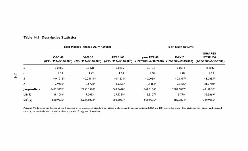
Table 14.1 Descriptive Statistics
Spot Market Indexes Daily Returns ETF Daily Returns
iSHARESCAC 40 DAX 30 FTSE 100 Lyxor ETF 40 DAXEX FTSE 100
(8/13/1993–6/30/2008) (7/8/1993–6/30/2008) (4/10/1992–6/30/2008) (1/22/2001–6/30/2008) (1/3/2001–6/30/2008) (4/28/2000–6/30/2008)
µ 0.0185 0.0328 0.0185 0.0133 0.0011 0.0032
σ 1.32 1.42 1.03 1.38 1.48 1.22
S 0.1215* 0.28111* 0.1831* 0.0089 0.1397* 1.2855*
K 2.9453* 3.6778* 3.2295* 3.413* 5.5375* 21.9750*
Jarque–Bera 1412.3195* 2253.3520* 1862.3610* 941.8184* 2501.6097* 43158.58*
LB(5) 18.1084* 7.0093 29.9359* 15.5127* 5.770 32.3469*
LB2(5) 828.9228* 1,224.1033* 903.3027* 590.0530* 385.9894* 349.9365*
Asterisk (*) denotes significance at the 1 percent level. µ, mean; σ, standard deviation; S, skewness; K, excess kurtosis; LB(5) and LB2(5) are the LjungBox statistics for returns and squaredreturns, respectively, distributed as chi-square with 5 degrees of freedom.
205

(φ1) is indicative of statistically insignificant positive feedback trading for alltests, thus implying that noise investors do not bear a decisive presence inour sample markets. Moreover, the φ0 coefficient is reflective of insignifi-cant first-order autocorrelation (whose sign switches from positive to negative in the aftermath of the introduction of ETFs), suggesting that the spot markets in the UK, France, and Germany are characterized byenhanced efficiency. Moving to the conditional variance process, we noticethat δ remains consistently positive and significant throughout our tests,thus suggesting that negative innovations tend to increase volatility morethan positive ones, something further confirmed when calculating theasymmetric ratio (β δ)/β.5 This volatility asymmetry appears more pro-nounced during the post-ETF period as indicated by the higher values of
206 Part I I i EXCHA NGE-TR ADED FUND STR ATEGIES
Table 14.2 Maximum Likelihood Estimates of the Sentana and Wadhwani(1992) Model: Pre- versus Post-ETF Spot Market Indexes Daily Returns
Conditional mean equation: rt α (φ0 φ1 σ 2t)rt1 θ σ 2
t εt
Conditional variance specification: σ 2t ω β ε2
t1 γσ2t1 δSt1 ε2
t1
Pre-ETF Post-ETF
CAC 40 DAX 30 FTSE 100 CAC 40 DAX 30 FTSE 100
α 0.0319 0.0314 0.0050 0.0218 0.0150 0.0141
(0.0605) (0.0452) (0.0298) (0.0265) (0.0289) (0.0231)
θ 0.0531 0.0271 0.0440 0.0238 0.0055 0.0160
(0.0434) (0.0329) (0.0403) (0.0181) (0.0172) (0.0248)
φ0 0.0551 0.0180 0.0762 0.0520 0.0196 0.0478
(0.0464) (0.0381) (0.0401) (0.0335) (0.0337) (0.0308)
φ1 0.1095 0.0058 0.0067 0.0017 0.0056 0.0126
(0.0224) (0.0142) (0.0331) (0.0109) (0.0085) (0.0144)
ω 0.0228 0.0279 0.0053 0.0247 0.0268 0.0160
(0.0065)* (0.0054)* (0.0015)* (0.0042)* (0.0045)* (0.0027)*
β 0.0161 0.0580 0.0164 0.0299 0.0170 0.0183
(0.0078) (0.0120)* (0.0080) (0.0067)* (0.0105) (0.0088)
γ 0.9432 0.9036 0.9544 0.9222 0.9149 0.9214
(0.0073)* (0.0111)* (0.05700)* (0.0094)* (0.0116)* (0.0103)*
δ 0.0500 0.0418 0.0459 0.1731 0.1670 0.1520
(0.0101)* (0.0131)* (0.0115)* (0.0159)* (0.0152)* (0.0119)*
(β δ)/β 4.1056 1.7190 3.7988 4.7893 8.8235 7.3060
Half-life 43.8020 39.0358 110.5566 32.4251 36.9183 32.8171

the δ coefficient (and the higher absolute values of the asymmetric ratio).6
What is more, volatility exhibits high persistence, as reflected through thestatistically significant γ coefficient, thus denoting the significant impact oflagged volatility over contemporaneous volatility. To illustrate this persist-ence, we calculate the volatility half-life as HL ln (0.5)/ ln(β γ δ/2),in line with Harris and Pisedtasalasai (2006). Our results indicate thatvolatility is highly persistent, with its persistence, however. exhibiting signsof decline in the post-ETF period for all markets.
Repeating the above analysis using the set of Equation (14.7) and Equation (14.8) to control for possible asymmetries in feedback tradingcontingent on market direction, we notice (Table 14.3) a consistently nega-tive (and insignificant) φ2 coefficient which reveals the absence of any suchasymmetries. As the rest of the estimates reported in Table 14.3 are similar
chapter 14 EXCHA NGE-TR ADED FUNDS and Noise Trading 207
Table 14.3 Maximum Likelihood Estimates of the Sentana and Wadhwani(1992) Model: Pre- versus Post-ETF Spot Market Indexes Daily Returns
Conditional mean equation: rt α (φ0 φ1 σ 2t)rt1 θσ 2
t φ2 |rt1| εt
Conditional variance specification: σ 2t ω β ε2
t1 γσ2t1 δ St1 ε2
t1
Pre-ETF Post-ETF
CAC 40 DAX 30 FTSE 100 CAC 40 DAX 30 FTSE 100
α 0.0178 0.0250 0.0103 0.0303 0.0121 0.0170
(0.0562) (0.0378) (0.0268) (0.0371) (0.0348) (0.0260)
θ 0.0691 0.0192 0.0541 0.0195 0.0039 0.0119
(0.0400) (0.0336) (0.0389) (0.0255) (0.0167) (0.0256)
φ0 0.0616 0.0158 0.0786 0.0542 0.0204 0.0488
(0.0478) (0.0340) (0.0335)* (0.0290) (0.0252) (0.0290)
φ1 0.0134 0.0050 0.0080 0.0014 0.0054 0.0125
(0.0217) (0.0140) (0.0280) (0.0077) (0.0048) (0.0012)
φ2 0.0426 0.0214 0.0206 0.0182 0.0065 0.0096
(0.0370) (0.0469) (0.0311) (0.0355) (0.0294) (0.0353)
ω 0.0235 0.0275 0.0054 0.0249 0.0269 0.0159
(0.0169) (0.0130) (0.0026) (0.0071)* (0.0063)* (0.0045)*
β 0.0162 0.0577 0.0167 0.0307 0.0171 0.0182
(0.0090) (0.0001)* (0.0075) (0.0122) (0.0086) (0.0060)*
γ 0.9419 0.9045 0.9539 0.9227 0.9149 0.9218
(0.0201)* (0.0224)* (0.0101)* (0.0126)* (0.0107)* (0.0141)*
Asterisk (*) denotes significance at the 1% level. Parentheses include the standard errors of the estimates.

to those reported previously in Table 14.2, this further confirms theabsence of significant feedback trading pre- and post-ETF and also showsthat the documented volatility asymmetries cannot be associated withasymmetries in the behavior of feedback traders.
To assess the significance of the difference in feedback trading betweenthe two periods, we run the specification proposed by Antoniou, Koutmos,and Pericli (2005)
(14.9)
(14.10)
where Dt 1 for the pre-ETF period and Dt 0 for the post-ETFperiod. As the β0 estimates in Table 14.4 reveal, the average level of volatil-ity appears to have significantly (insignificantly, in the case of Germany)declined post-ETF, a fact in line with the reduction in volatility persistenceillustrated in Tables 14.2 and 14.3. What is more, feedback trading is foundto be insignificant prior to and after the launch of the ETF segment in allthree markets with its presence being insignificantly different between thetwo periods. The φ0 coefficient furnishes us with the same sign-switchreported in the previous tests (positive pre-, negative post-ETF), andappears significant only in the case of the German market post-ETF;results from the t statistics support its significant period-to-period differ-ence in the case of the UK and France.
We finally turn our attention to the ETF level and repeat our tests forthe ETF series of our sample. According to Table 14.5, there is no evidenceof significance surrounding feedback trading here either. Much like inTables 14.214.4, results here confirm the presence of highly persistentand asymmetric volatility while all ETFs are characterized by insignifi-cantly negative first-order autocorrelation, similar to the post-ETF esti-mates reported for spot indexes.
As the previous results indicate, Europe’s three largest capital marketsappear to accommodate largely insignificant feedback trading during the lastcouple of decades. The introduction of ETFs did little to change this, moreso since feedback traders are found to be insignificant in that market seg-ment as well. Although the advent of ETFs has coincided with structural
208 Part I I i EXCHA NGE-TR ADED FUND STR ATEGIES
R D D R Dt t t t t t= + σ + + − + +−α θ φ φ φ φ20 1 0 2 1 1 11[ ( )] [, , , 11 2 11. ( )]− σ + ε2
−D Rt t t
σ = + − + σ + ε + δ− −12
−t t t t t tD D S20 1 0 2 1 1
22 11β β β β, , ( ) εε −1
2t
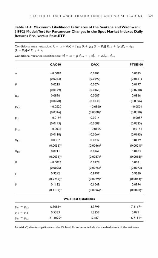
chapter 14 EXCHA NGE-TR ADED FUNDS and Noise Trading 209
Table 14.4 Maximum Likelihood Estimates of the Sentana and Wadhwani(1992) Model:Test for Parameter Changes in the Spot Market Indexes DailyReturns Pre- versus Post-ETF
Conditional mean equation: Rt α θσ 2t [φ 0,1 Dt φ0,2 (1 Dt)] Rt1 [φ1,1Dt φ1,2
(1 Dt)]σ2 Rt1 εt
Conditional variance specification: σ 2t ω β ε2
t1 γ σ2t1 δ St1 ε 2
t1
CAC40 DAX FTSE100
α 0.0086 0.0303 0.0025
(0.0253) (0.0290) (0.0181)
θ 0.0215 0.0074 0.0197
(0.0179) (0.0163) (0.0218)
φ0,1 0.0896 0.0087 0.0866
(0.0420) (0.0330) (0.0396)
φ0,2 0.0520 0.0520 0.0501
(0.0346) (0.0000)* (0.0310)
φ1,1 0.0197 0.0014 0.0057
(0.0193) (0.0088) (0.0325)
φ1,2 0.0037 0.0105 0.0151
(0.0110) (0.0064) (0.0145)
β0,1 0.0387 0.0347 0.0139
(0.0055)* (0.0046)* (0.0021)*
β0,2 0.0211 0.0262 0.0103
(0.0031)* (0.0037)* (0.0018)*
β 0.0026 0.0278 0.0071
(0.0026) (0.0075)* (0.0072)
γ 0.9242 0.8997 0.9280
(0.9242)* (0.0079)* (0.0064)*
δ 0.1132 0.1049 0.0994
(0.1132)* (0.0096)* (0.0090)*
Wald Test t statistics
φ 0,1 φ 0,2 6.8081* 3.3799 7.4167*
φ1,1 φ1,2 0.5333 1.2259 0.0711
φ 0,1 φ 0,2 21.4075* 5.687 6.7111*
Asterisk (*) denotes significance at the 1% level. Parentheses include the standard errors of the estimates.

changes in spot volatility dynamics (decline of average volatility levels,increase in volatility asymmetries, and decrease in its persistence), the factremains that the spot markets in Europe’s major stock exchanges exhibitsigns of enhanced efficiency and are dominated by rational investors bothbefore and after the ETF launch. The fact that this appears to be the case inthe ETF segments as well is particularly encouraging from a regulatoryviewpoint, as it suggests that ETFs have thus far managed to serve theiroriginal purpose, namely, contribute towards the completeness and efficiencyof these markets. In view of the above results—and given that the ETFindustry has already begun to take off in emerging markets in recentyears—it would be worth extending the present study by investigating in thefuture (as more data becomes available with time) how the introduction ofETFs impacts on noise trading in these markets as well, more so given thedifferential conditions typifying their institutional frameworks compared totheir developed counterparts.
210 Part I I i EXCHA NGE-TR ADED FUND STR ATEGIES
Table 14.5 Maximum Likelihood Estimates of the Sentana and Wadhwani(1992) Model: ETF Daily Returns
Conditional mean equation: rt α (φ0 φ1 σ 2t )rt1 θσ 2
t εt
Conditional variance specification: σ 2t ω βε2
t1 γσ 2t1 δSt1 ε 2
t1
Lyxor ETF iSHARESCAC 40 DAXEX FTSE 100
α 0.1272 0.0106 0.0032
(0.0271) (0.0298) (0.0240)
θ 0.0184 0.0235 0.0035
(0.0187) (0.0170) (0.0252)
φ0 0.0521 0.0251 0.0717
(0.0338) (0.0325) (0.0283)*
φ1 0.0016 0.0115 0.0101
(0.0109) (0.0078) (0.0082)
ω 0.0253 0.0301 0.0155
(0.0044)* 0.0042) (0.0027)*
β 0.0275 0.0190 0.0035
(0.0075)* (0.0401)* (0.0081)
γ 0.9519 0.9200 0.9183
(0.0099)* (0.0117)* (0.0087)*
δ 0.1811 0.1536 0.1331
(0.0169)* (0.0134)* (0.0113)*
Asterisk (*) denotes significance at the 1% level. Parentheses include the standard errors of the estimates.

REFERENCES
Antoniou, A., Koutmos, G., and Pericli, A. (2005) Index Futures and Posi-tive Feedback Trading: Evidence from Major Stock Exchanges. Journalof Empirical Finance, 12(2): 219238.
Bollerslev, T., Engle, R.F., and Nelson, D. (1994) ARCH Models. In Engle,R.F. and McFadden, D.L. (eds.), Handbook of Econometrics. Burlington,MA: Elsevier.
De Long, J.B., Shleifer, A., Summers, L.H., and Waldmann, R.J. (1990)Positive Feedback Investment Strategies and Destabilizing RationalSpeculation. Journal of Finance, 45(2): 379–395.
Deville, L. (2008) Exchange-Traded Funds: History, Trading and Research.In: Zopounidis, C., Doumpos, M., and Pardalos, P.M. (eds.), Handbookof Financial Engineering, New York: Springer.
Glosten, L., Jagannathan, R., and Runkle, D. (1993) On the Relationbetween the Expected Value and the Volatility of the Nominal ExcessReturn on Stocks. Journal of Finance, 48(5): 1779–1801.
Harris, R.D.F. and Pisedtasalasai, A. (2006) Return and Volatility Spilloversbetween Large and Small Stocks in the UK. Journal of Business Financeand Accounting, 33(9–10): 1556–1571.
Sentana, E. and Wadhwani, S. (1992) Feedback Traders and Stock ReturnAutocorrelations: Evidence from a Century of Daily Data. EconomicJournal, 102(411): 415–425.
NOTES
1. Available at: http://www.ici.org/stats/etf/etfs_03_09.html
2. This “migration-hypothesis” was formally tested (Antoniou, Koutmos,and Pericli, 2005) in the case of index futures’ introduction with resultslargely refuting it.
3. Since the market indexes mentioned here have been with us at leastsince the 1970s, the pre-ETF introduction period would have been dis-proportionately large compared with the post ETF one.
4. With the exception of the DAX index and its corresponding ETF.
5. As Antoniou, Koutmos, and Pericli (2005) show, the contribution of apositive innovation is reflected in β while the contribution of a negative
chapter 14 EXCHA NGE-TR ADED FUNDS and Noise Trading 211

innovation by the sum of β δ. An asymmetric ratio value greaterthan unity (in absolute terms) would thus suggest that negative innova-tions contribute more to market volatility than positive ones.
6. The switch in the sign of the asymmetric ratio post-ETF is due to thedirectional change of volatility autocorrelation between the two sub-periods; more specifically, contemporaneous volatility is found toincrease with lagged squared innovations pre-ETF, yet the inverseoccurs post-ETF as the switch in the sign of the volatility autocorrela-tion coefficient (β) in Table 14.2 indicates.
212 Part I I i EXCHA NGE-TR ADED FUND STR ATEGIES

213
15C H A P T E R
Penetrating Fixed-Income Exchange-Traded Funds
Gerasimos G. Rompotis
ABSTRACT
This chapter investigates various issues concerning the performance, thetrading premium, and trading activity of fixed-income exchange-tradedfunds (ETFs). Findings first indicate that ETFs slightly underperform theirtracking indexes. Moreover, the results indicate that ETFs trade daily, onaverage, at a premium to their net asset value. Regression analysis revealsthat the premium is strongly persistent on a daily basis. Further regressionanalysis demonstrates that the premium is meaningful in determiningfuture returns. In particular, return is found to be positively and negativelyaffected by the contemporaneous and lagged premium, respectively. Finally,evidence on the positive relationship between trading volume and laggedintraday volatility and premium are revealed.
INTRODUCTION
Apart from the equity-linked exchange-traded funds (ETFs), new types ofETFs allocating funds in nonequity investments are now available. One significant category of these new ETFs is the fixed-income ETFs. Fixed-income ETFs track the performance of fixed-income securities. In a stockETF, the fund is generally composed of all the stocks in the index. However,

this is not the case in most bond ETFs. The fund holds a fraction of thebonds that make up the underlying index. Bond prices are relatively straight-forward being a function of the risk-free rate, the coupon, the quality of thebond, and the years to maturity.
Fixed-income ETFs may track broad bond market indexes containing abroad mix of both government and corporate bonds at different maturities.Furthermore, fixed-income ETFs may invest in treasury bonds based ondifferent maturities along the yield curve. Moreover, there are the treasuryinflation protected securities ETFs (TIPS) which pay interest equal to theConsumer Price Index (CPI) plus a premium. They provide a hedge againstinflation and are designed to outperform regular bonds when inflationexpectation rises. Another type of fixed-income ETFs relates to those thatinvest in different asset classes allowing investors to get a fully diversifiedportfolio by just buying an ETF. Finally, there is the target date or lifecycleETFs that target the defined contribution pension plan market. Target datefunds are similar to balanced asset allocation funds having one additionalfeature, namely, they become more conservative as they approach the targetdate. Funds reduce risk by selling stocks and buying bonds as the targetdate approaches.
Bond ETFs can be as liquid and transparent as stock ETFs, offeringinvestors the flexibility of trading stocks along with the benefits on invest-ing in bonds. Fixed-income ETFs moves just like stocks, they can be intra-day traded and can be sold short at any time throughout the trading day. In contrast, bond mutual funds only trade at the end of the trading day,making the bond ETF more liquid than a bond mutual fund.
The main similarities between bonds and fixed-income ETFs are thatthey are affected by the same factors such as the fluctuations in interestrates, variations in yield spreads, and changes in yield curves. The effects ofinterest rates on bond prices are especially severe during the periods offinancial and banking crisis. As a matter of fact, the current crisis hasresulted in increases in the “spreads” or the premium which large corpora-tions pay to borrow money by issuing bonds to investors. On the otherhand, the basic differences between fixed-income ETFs and bonds are thatthe ETFs usually distribute dividends on a monthly basis, while bonds usu-ally pay interest twice a year. Furthermore, bond ETFs have no maturitydate while bonds do. In addition, the income received by ETFs on thebonds included in their portfolio are reinvested in new bonds rather thanreturned to investors. Moreover, ETFs trade on stock exchanges, whereas
214 Part I I i EXCHA NGE-TR ADED FUND STR ATEGIES

bonds are generally bought and sold through dealer firms. Finally, individ-ual investors can execute active trading strategies with ETFs that may bedifficult to apply by using bonds themselves. Short selling is such an exam-ple. The same patterns apply when comparing bond ETFs with open-endedfixed-income mutual funds.
Going further, there are differences between ETFs and open-endedfixed-income mutual funds. Apart from the trading on stock exchanges andthe execution of active investing strategies and intraday trading orders men-tioned above, ETF investors pay transaction fees to brokerage firms whilemutual fund investors do not. In addition, with mutual funds investors paypurchase and redemption fees when they enter or exit the fund, while ETFinvestors do not have to pay such fees. Moreover, the majority of open-ended mutual funds are actively managed and, as a result, they tend toimpose higher management fees than the passively managed ETFs. Apartfrom their unique advantages, the fixed-income ETFs are also subject tosome significant weaknesses (described in Mazzilli, Maister, and Perlman(2008)). One disadvantage is that the bond ETFs do not mature, whichmeans that when an investor decides to redeem their ETF shares, it may beat a price that is lower than the initial investment. In addition, the determi-nation of the exact yield for fixed-income ETFs can be difficult. Trackingfailure is another potential disadvantage of bond ETFs, while noncurrenttrading hours may also occur between the bond ETFs and their holdings.
In this chapter, we examine various issues concerning the performance offixed-income ETFs, the replication efficiency, the premium, the relation-ship between premium and return, and the determinative factors of tradingactivity. At first, the results show that fixed-income ETFs underperformtheir benchmarks. Going further, the findings demonstrate that fixed-income ETFs trade, on average, at a persistent premium to their net assetvalue (NAV). Regression analysis reveals that the premium is indicative offuture returns. Finally, evidence of the positive relationship between trad-ing volume and lagged intraday volatility and premium is found.
METHODOLOGY
Performance and Risk
Returns of ETFs are calculated using both their NAV and the tradingprices. Daily returns are estimated in percentage terms, while the risk is thestandard deviation of daily returns. A second performance measure we
chapter 15 PENETR ATING FIXED-INCOME EXCHA NGE-TR ADED FUNDS 215

apply is tracking error, which indicates the return difference between ETFsand indexes. Two tracking error measures are employed. The first one(TE1) concerns the difference in returns between ETFs and indexes and the second one (TE2) estimates tracking error as the standard devia-tion in return differences between ETFs and indexes (found in Frino andGallagher, 2001).
Premium and Persistence of Premium
We first estimate premium as the dollar difference between the closingprice and NAV and then as the percentage deviation between ETF closingprices and NAVs. In general, one key feature of ETFs is the chances theyoffer institutional investors to execute profitable arbitrage strategies, whichin turn contribute to the sharp elimination of premiums or discounts intrading prices. To verify this argument, we search for persistence patternsin fixed-income ETF premiums. We follow the approach of Elton et al.(2002) and regress the premium (either the dollar or the percentage) ofiShares on day t against the premium on day t 1. The model we apply isrepresented in Equation (15.1).
Premiumt α β Premiumt1 ε (15.1)
Explaining Return
According to Jares and Lavin (2004), there is a significant connectionbetween return and premium for Japan and Hong Kong iShares. Morespecifically, the authors find a strong and significantly negative relationshipbetween return and contemporaneous premium and a significantly positiverelation between return and lagged premium. On the contrary, Cherry(2004) finds that ETF return is negatively related to lagged premium. Thefindings of these studies suggest that premiums are meaningful for thedetermination of future returns of ETFs.
We investigate the relation between the premium and return of fixed-income ETFs, applying a time-series regression of each ETF return on thecontemporaneous and lagged premium (premium on day t and day t 1,respectively). The model we estimate is shown in Equation (15.2).
Returnt α β1 Premiumt β2 Premiumt1 ε (15.2)
216 Part I I i EXCHA NGE-TR ADED FUND STR ATEGIES

Explaining Volume
Elton et al. (2002) demonstrate that the trading volume of Standard &Poor’s Depositary Receipts (SPDRs), which track the S&P 500 Index, is significantly affected by the lagged premium and lagged intraday volatilityestimated as the fraction of the intraday highest price minus the intradaylowest price of the tracking index divided by the closing price of index.Lagged values of volatility and premium are considered since the differencebetween the price and NAV is calculated at the end of the day and, there-fore, the difference signals (if any) arbitrage opportunities the next day.
We search whether Elton et al. (2002) regression analysis of volumeapplies to fixed-income ETFs by using the intraday volatility of ETFsthemselves and not the intraday price volatility of indexes. The model weapply is represented by Equation (15.3).
LnVolumet α β1 Volatilityt1 β2 Premiumt1 ε (15.3)
DATA AND STATISTICS
In this chapter we use ETF trading data that cover the period July 29, 2002to February 27, 2009. Our data consists of the closing prices, which are the4 p.m. bid/ask midpoint, and the NAVs of a sample of 35 fixed-income Bar-clay’s iShares. The 22 ETFs of the sample are bond funds tracking variousbroad market, treasury, government credit, credit, municipal, mortgage,and international bond indexes; and 13 are specialty ETFs which track vari-ous asset allocation, target date (pension market), and preferred stockindexes. The closing prices of iShares were gathered from Nasdaq.com.Nasdaq.com also provided us with the daily volumes of ETFs. The dailyNAVs were found on the Website of iShares (www.us.ishares.com).
Table 15.1 reports information concerning the symbol of the sample’sETFs, name, type, inception date, expense ratio, intraday volatility, andaverage daily volume. The average expense ratio of ETFs is equal to 24 bpsreflecting the low managerial expenses charged by ETFs as a result of theirpassive investing character. Furthermore, the average intraday volatility isequal to 1.281 percent, while the average daily volume approximates the116,000 shares. However, it should be noted that there are significant varia-tions among the individual average volumes. Indicatively, the maximumaverage daily volume of the sample amounts to 1.3 million shares while theminimum volume is equal to 383 shares.
chapter 15 PENETR ATING FIXED-INCOME EXCHA NGE-TR ADED FUNDS 217

Table 15.1 Profiles of ETFs
The following exhibit presents the profiles of ETFs which, are the symbol, name, investing style (type), inception date, expense ratio, intraday volatilityestimated (as the fraction of the ETFs’ intraday highest trading price minus the intraday lowest trading price divided by the closing price), and the averagedaily volume in number of shares.
Inception Expense IntradaySymbol Name Type Date Ratio (%) Volatility (%) Volume
AGG Barclays Aggregate Bond Fund Broad Market 09/22/2003 0.24 0.446 298,903
SHY Barclays 1–3 Year Treasury BF Treasury 07/22/2002 0.15 0.152 528,736
IEI Barclays 3–7 Year Treasury BF Treasury 01/05/2007 0.15 0.381 70,527
IEF Barclays 7–10 Year Treasury BF Treasury 07/22/2002 0.15 0.463 246,674
TLH Barclays 10–20 Year Treasury BF Treasury 01/05/2007 0.15 0.640 17,674
TLT Barclays 20 Year Treasury BF Treasury 07/22/2002 0.15 0.799 1,332,332
AGZ Barclays Agency Bond Fund Treasury 11/05/2008 0.20 0.574 9,461
SHV Barclays Short Treasury Bond Fund Treasury 01/05/2007 0.15 0.087 156,532
TIP Barclays TIPS Bond Fund Treasury 12/04/2003 0.20 0.512 273,241
GBF Barclays Government/Credit BF Government Cred 01/05/2007 0.20 0.384 11,894
GVI Barclays Intermediate Gov/Cred BF Government Cred 01/05/2007 0.20 0.457 13,124
HYG iBoxx $ High Yield Corporate BF Credit 04/04/2007 0.50 1.390 189,243
LQD iBoxx $ Investment Grade Corp BF Credit 07/22/2002 0.15 0.682 239,435
CSJ Barclays 1–3 Year Credit BF Credit 01/05/2007 0.20 0.500 44,727
CFT Barclays Credit Bond Fund Credit 01/05/2007 0.20 0.692 12,247
CIU Barclays Intermediate Credit BF Credit 01/05/2007 0.20 0.570 24,694
CMF S&P California Municipal BF Municipal Bond 10/04/2007 0.25 0.838 8,073
218

MUB S&P National Municipal BF Municipal Bond 09/07/2007 0.25 0.963 71,118
NYF S&P New York Municipal BF Municipal Bond 10/04/2007 0.25 0.653 2,765
SUB S&P Short Term National Mun BF Municipal Bond 11/05/2008 0.25 0.667 8,063
MBB Barclays MBS Bond Fund Mortgage 03/13/2007 0.36 0.498 60,660
EMB JPMorgan USD Emerg Markets BF International 12/17/2007 0.60 1.371 16,117
AOA S&P Aggressive Allocation Fund Allocation 11/04/2008 0.34 4.523 30,024
AOK S&P Conservative Allocation Fund Allocation 11/04/2008 0.31 2.256 6,880
AOR S&P Growth Allocation Fund Allocation 11/04/2008 0.33 3.558 26,458
AOM S&P Moderate Allocation Fund Allocation 11/04/2008 0.32 3.472 9,305
TZD S&P Target Date 2010 Index Fund Target Date 11/04/2008 0.31 5.266 383
TZE S&P Target Date 2015 Index Fund Target Date 11/04/2008 0.31 0.262 411
TZG S&P Target Date 2020 Index Fund Target Date 11/04/2008 0.31 0.273 505
TZI S&P Target Date 2025 Index Fund Target Date 11/04/2008 0.31 0.874 8,402
TZL S&P Target Date 2030 Index Fund Target Date 11/04/2008 0.30 0.237 1,595
TZO S&P Target Date 2035 Index Fund Target Date 11/04/2008 0.30 1.596 556
TZV S&P Target Date 2040 Index Fund Target Date 11/04/2008 0.29 1.528 500
TGR S&P Target Date Retir Income IF Target Date 11/04/2008 0.31 4.554 952
PFF S&P U.S. Preferred Stock IF Preferred Stock 03/26/2007 0.48 2.703 332,473
Average 0.24 1.281 115,848
219

EMPIRICAL RESULTS
Performance and Risk
Table 15.2 presents the average returns and risks of ETFs and indexes.The average NAV return is negative and equal to minus 5.2 bps. The corresponding average return of indexes is equal to minus 3.8 bps. Com-paring average returns, we infer that the ETFs slightly underperform theirbenchmarks. The underperformance of fixed-income ETFs revealed byour findings is consistent with the respective underperformance reportedby Svetina and Wahal (2008). When it comes to risk, results show thatthere is no significant difference between the volatility of ETFs andindexes. Considering the price returns, the results indicate that the ETFsstill underperform the indexes. More specifically, the average return ofETFs is equal to 4.3 bps. With regard to risk, the average standard deviation of price returns is equal to 1.174, being higher than the corre-sponding risk estimation of indexes, which is equal to 0.944.
The next exhibit presents the return and risk calculations of ETFs andthe tracking indexes. Return is the average daily return and risk is the stan-dard deviation of daily return. Calculations are presented in two verticalpanels. Panel A presents returns and risks when NAVs are used, while PanelB presets returns and risks in trading prices terms. N represents the num-ber of daily observations.
Tracking errors are displayed in Table 15.3. The average TE1 of ETFsis equal to 1.4 bps. Considering the statistical significance of trackingerror estimates, the applied t tests indicate that the estimates are significantfor 17 out of 35. The TE2 of ETFs in NAV terms is equal to 11.5 bps.With respect to price returns, the average TE1 is essentially equal to zerowhile only 8 out of the 35 individual tracking error estimates are statisti-cally indifferent from zero. However, the average TE2 of ETFs is consider-able being equal to 1.215 showing that the difference between the pricereturns of ETFs and indexes are more volatile relative to the correspondingrelationship in NAV terms.
Premium and Persistence of Premium
Table 15.4 presents the average daily premiums of ETFs. The standard devi-ation in daily premiums is also reported in the exhibit. Results demonstratethat, on average, the fixed-income ETFs trade at a premium to their NAV.
220 Part I I i EXCHA NGE-TR ADED FUND STR ATEGIES
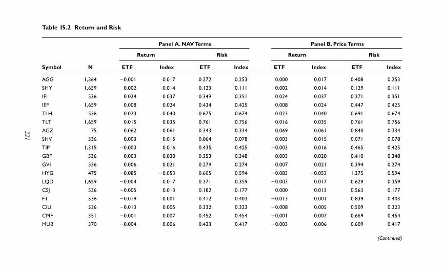
Table 15.2 Return and Risk
Panel A. NAV Terms Panel B. Price Terms
Return Risk Return Risk
Symbol N ETF Index ETF Index ETF Index ETF Index
AGG 1,364 0.001 0.017 0.272 0.253 0.000 0.017 0.408 0.253
SHY 1,659 0.002 0.014 0.123 0.111 0.002 0.014 0.129 0.111
IEI 536 0.024 0.037 0.349 0.351 0.024 0.037 0.371 0.351
IEF 1,659 0.008 0.024 0.434 0.425 0.008 0.024 0.447 0.425
TLH 536 0.023 0.040 0.675 0.674 0.023 0.040 0.691 0.674
TLT 1,659 0.015 0.035 0.761 0.756 0.016 0.035 0.761 0.756
AGZ 75 0.062 0.061 0.343 0.334 0.069 0.061 0.840 0.334
SHV 536 0.003 0.015 0.064 0.078 0.003 0.015 0.071 0.078
TIP 1,315 0.003 0.016 0.435 0.425 0.003 0.016 0.465 0.425
GBF 536 0.003 0.020 0.353 0.348 0.003 0.020 0.410 0.348
GVI 536 0.006 0.021 0.279 0.274 0.007 0.021 0.394 0.274
HYG 475 0.085 0.053 0.605 0.594 0.083 0.053 1.375 0.594
LQD 1,659 0.004 0.017 0.371 0.359 0.003 0.017 0.629 0.359
CSJ 536 0.005 0.013 0.182 0.177 0.000 0.013 0.563 0.177
FT 536 0.019 0.001 0.412 0.403 0.013 0.001 0.839 0.403
CIU 536 0.013 0.005 0.332 0.323 0.008 0.005 0.509 0.323
CMF 351 0.001 0.007 0.452 0.454 0.001 0.007 0.669 0.454
MUB 370 0.004 0.006 0.423 0.417 0.003 0.006 0.609 0.417
(Continued)
221

Table 15.2 (Continued)
Panel A. NAV Terms Panel B. Price Terms
Return Risk Return Risk
Symbol N ETF Index ETF Index ETF Index ETF Index
NYF 351 0.003 0.010 0.446 0.493 0.004 0.010 0.764 0.493
SUB 75 0.028 0.032 0.103 0.359 0.042 0.032 1.232 0.359
MBB 492 0.008 0.029 0.322 0.309 0.009 0.029 0.374 0.309
EMB 299 0.063 0.038 0.983 0.920 0.059 0.038 1.547 0.920
AOA 75 0.198 0.189 2.802 2.809 0.204 0.189 2.764 2.809
AOK 75 0.050 0.043 0.693 0.692 0.027 0.043 2.034 0.692
AOR 73 0.115 0.106 1.873 1.878 0.064 0.106 3.466 1.878
AOM 75 0.098 0.090 1.187 1.189 0.066 0.090 2.730 1.189
TZD 75 0.090 0.080 1.221 1.220 0.061 0.080 0.908 1.220
TZE 75 0.116 0.105 1.495 1.499 0.088 0.105 1.302 1.499
TZG 75 0.141 0.130 1.773 1.774 0.115 0.130 1.241 1.774
TZI 75 0.164 0.153 2.029 2.035 0.135 0.153 1.786 2.035
TZL 75 0.188 0.175 2.295 2.298 0.193 0.175 1.785 2.298
TZO 75 0.205 0.194 2.511 2.512 0.209 0.194 1.938 2.512
TZV 75 0.217 0.205 2.639 2.641 0.183 0.205 2.269 2.641
TGR 75 0.064 0.053 0.947 0.951 0.042 0.053 2.100 0.951
PFF 482 0.159 0.135 2.715 2.690 0.164 0.135 2.677 2.690
Average 499 0.052 0.038 0.940 0.944 0.043 0.038 1.174 0.944
222

chapter 15 PENETR ATING FIXED-INCOME EXCHA NGE-TR ADED FUNDS 223
Table 15.3 Tracking Error of ETFs
The following exhibit presents the calculations of ETF tracking error, which represents thedifference in performance between ETFs and tracking indexes. Two alternative tracking errorestimations are used. The first one (TE1) concerns the average raw return difference betweenETFs and indexes and the second one (TE2) estimates tracking error as the standard deviationsin daily return differences between ETFs and indexes. In addition, t test values on the statisticalsignificance of raw returns’ difference are presented. Calculations are presented in two verticalpanels. Panel A presents tracking error when NAV returns are used in estimating ETF returns,while Panel B shows tracking error when ETF returns are calculated in trading price terms.
Panel A. NAV Terms Panel B. Price Terms
Symbol TE1 t Test TE2 TE1 T-test TE2
AGG 0.018* 6.262 0.104 0.017‡ 1.856 0.339SHY 0.012* 8.531 0.057 0.012* 6.078 0.081IEI 0.014* 4.516 0.070 0.014‡ 1.749 0.180IEF 0.016* 7.788 0.083 0.016* 3.876 0.166TLH 0.018* 3.739 0.109 0.017 1.509 0.269TLT 0.019* 7.648 0.103 0.019* 3.159 0.247AGZ 0.001 0.093 0.101 0.008 0.087 0.785SHV 0.012* 2.943 0.093 0.012* 2.708 0.102TIP 0.019* 7.046 0.099 0.019* 2.970 0.229GBF 0.017* 4.086 0.095 0.016 1.111 0.339GVI 0.015* 4.217 0.084 0.013 0.971 0.320HYG 0.032* 4.723 0.148 0.030 0.502 1.326LQD 0.021* 8.147 0.105 0.020 1.575 0.519CSJ 0.018* 4.493 0.093 0.013 0.536 0.575CFT 0.020* 3.747 0.123 0.013 0.394 0.786CIU 0.018* 3.857 0.109 0.013 0.656 0.454CMF 0.008 1.114 0.137 0.008 0.260 0.586MUB 0.010 1.352 0.140 0.009 0.332 0.513NYF 0.013 1.093 0.223 0.006 0.126 0.854SUB 0.004 0.092 0.344 0.011 0.070 1.302MBB 0.021* 4.805 0.095 0.020‡ 1.762 0.252EMB 0.025 2.631 0.163 0.020 0.253 1.395AOA 0.009 0.935 0.086 0.015 0.052 2.447AOK 0.007 1.087 0.054 0.015 0.067 2.005AOR 0.009 0.910 0.085 0.042 0.113 3.167AOM 0.008 0.911 0.074 0.024 0.080 2.578TZD 0.010 1.016 0.087 0.018 0.108 1.448TZE 0.011 1.033 0.092 0.018 0.078 1.973TZG 0.011 1.032 0.092 0.015 0.712 1.830TZI 0.011 0.990 0.098 0.018 0.057 2.689TZL 0.012 1.049 0.102 0.017 0.056 2.681TZO 0.012 0.969 0.105 0.016 0.039 3.482TZV 0.012 0.955 0.107 0.021 0.055 3.381TGR 0.011 1.114 0.084 0.011 0.044 2.219PFF 0.024‡ 1.949 0.274 0.029 0.638 0.999
Average 0.014 3.048 0.115 0.005 0.906 1.215
* Significant at the 1% level. †Significant at the 5% level. ‡Significant at the 10% level.

224 Part I I i EXCHA NGE-TR ADED FUND STR ATEGIES
Table 15.4 Premium in Prices of ETFs
This next exhibit presents the calculations of ETF average daily premium along with thestandard deviation of daily premium. Premium is estimated both in dollar terms, by subtractingthe closing NAV of ETFs on day t from the closing trading price on the same day, and inpercentage terms, by dividing the difference between the closing trading price and closing NAVby the closing NAV. Calculations are presented in two vertical panels. Panel A presents thepecuniary premium and Panel B presents the percentage premium.
Panel A. Pecuniary Premium Panel B. Percentage Premium
Symbol Average Standard Deviation Average Standard Deviation
AGG 0.309 0.469 0.305 0.476SHY 0.042 0.038 0.052 0.046IEI 0.064 0.135 0.061 0.125IEF 0.040 0.096 0.048 0.110TLH 0.077 0.215 0.072 0.199TLT 0.043 0.161 0.048 0.169AGZ 0.390 0.668 0.370 0.650SHV 0.069 0.039 0.063 0.035TIP 0.203 0.314 0.201 0.325GBF 0.395 0.569 0.386 0.562GVI 0.445 0.609 0.433 0.594HYG 1.510 1.609 1.754 2.185LQD 0.488 0.738 0.470 0.776CSJ 0.869 1.078 0.880 1.114CFT 0.927 0.948 0.972 1.056CIU 0.922 1.072 0.957 1.155CMF 0.793 1.134 0.793 1.175MUB 0.627 0.840 0.646 0.896NYF 0.987 1.504 1.018 1.630SUB 0.689 1.014 0.670 0.978MBB 0.157 0.218 0.154 0.212EMB 1.194 1.761 1.316 2.175AOA 0.108 0.403 0.472 1.800AOK 0.101 0.320 0.402 1.292AOR 0.209 0.631 0.889 2.682AOM 0.153 0.446 0.629 1.843TZD 0.263 0.498 1.106 2.087TZE 0.289 0.506 1.225 2.144TZG 0.186 0.422 0.803 1.805TZI 0.010 0.560 0.020 2.392TZL 0.061 0.793 0.209 3.387TZO 0.151 0.691 0.733 3.064TZV 0.206 0.662 0.955 2.914TGR 0.019 0.719 0.048 2.856PFF 0.192 0.325 0.590 1.065
Average 0.372 0.634 0.548 1.314

The average dollar premium is equal to 37.2 cent while the respective per-centage premium is equal to 0.548 percent. The respective premium’svolatilities are equal to 0.634 and 1.314. Earlier findings of the literature onequity ETFs also reveal that ETFs trade at prices that are different fromtheir NAV. In particular, Hughen (2003) reports that Malaysia iShares tradeat a premium to its net value. Jares and Lavin (2004) find similar results forthe Japan and Hong Kong iShares. On the contrary, Elton et al. (2002)report that SPDRs trade at a discount to its NAV.
The results of the regression analysis are reported in Table 15.5. Theaverage slope coefficient for the dollar premium is positive and equal to 0.486. The majority of individual betas (27 out of 35 beta estimates) arepositive and significant. The same pattern applies to the percentage pre-mium. The average beta estimate is equal to 0.489 while 26 single beta coefficients are positive and significant at the 10 percent level or better.Overall, our results contrast those of Elton et al. (2002) and indicate that thepremium of fixed-income ETFs is sufficiently persistent on a daily basis,implying limitations to the execution of arbitrage.
Explaining Return
Table 15.6 provides the results of Equation (15.2) on the relationshipbetween return and premium. Results provide sound evidence on the posi-tive relationship between return and contemporaneous premium and thenegative impact of lagged premium on return. The average estimate of con-temporaneous premium is equal to 0.781, while all the single estimationsare positive and statistically significant. The positive average estimationimplies that an increase in contemporaneous premium by 1 unit results inan increase in ETF return by 0.781 percent on the same day.
With respect to the relationship between the lagged premium and return,the results provide strong evidence on the negative correlation betweenthese two factors. The relevant average coefficient of the model is equal to0.664. In addition, the majority of the single estimates are negative (onlyone is positive but insignificant) while 31 out of the 34 negative estimationsare significant. Our findings are in line with the ones reported by Cherry(2004) about equity ETFs (he estimates an average beta of 0.680). Overall,our results make us reject the efficient market hypothesis for fixed-incomeETFs and reveal possible opportunities for investors to exploit the premiumin ETF trading prices and execute profitable arbitrage strategies.
chapter 15 PENETR ATING FIXED-INCOME EXCHA NGE-TR ADED FUNDS 225

Table 15.5 Persistence in Premium
The following exhibit presents the results of a time-series regression model which searches for persistence patterns in iShares’ premium. Specifically, thepremium of ETFs on day t 1 is regressed on the premium on day t. Model is applied to the pecuniary premium (Panel A) and the percentage premium(Panel B).
Panel A. Pecuniary Premium Panel B. Percentage Premium
Symbol Alpha t Test Beta t Test R–sq Alpha t Test Beta t Test R2
AGG 0.029 1.404 0.907* 16.468 0.603 0.028 1.386 0.907* 16.284 0.603
SHY 0.033* 19.403 0.217* 5.963 0.047 0.040* 19.719 0.219* 6.191 0.048
IEI 0.055* 8.632 0.139* 3.235 0.019 0.053* 8.835 0.134* 3.133 0.018
IEF 0.038* 10.501 0.074 1.207 0.005 0.044* 10.717 0.073 1.203 0.005
TLH 0.070* 7.056 0.089 1.307 0.008 0.066* 7.172 0.081 1.211 0.007
TLT 0.042* 10.381 0.034 0.808 0.001 0.047* 10.736 0.024 0.619 0.001
AGZ 0.316* 3.558 0.204‡ 1.776 0.042 0.298* 3.473 0.208‡ 1.808 0.043
SHV 0.053* 8.164 0.236† 2.430 0.056 0.048* 8.208 0.236† 2.434 0.056
TIP 0.044* 3.561 0.784* 13.477 0.614 0.041* 3.337 0.796* 13.623 0.633
GBF 0.068† 2.609 0.829* 15.988 0.687 0.068† 2.545 0.825* 15.348 0.681
GVI 0.062† 2.672 0.863* 20.544 0.744 0.062† 2.627 0.860* 19.889 0.739
HYG 0.312† 2.290 0.791* 10.641 0.622 0.312† 2.141 0.820* 12.014 0.668
LQD 0.099† 2.235 0.797* 10.236 0.636 0.096† 2.091 0.795* 9.547 0.633
CSJ 0.119† 2.579 0.867* 18.454 0.751 0.119† 2.587 0.868* 18.784 0.753
CFT 0.253* 2.732 0.730* 8.840 0.531 0.268† 2.584 0.728* 8.344 0.528
CIU 0.074† 2.179 0.924* 25.946 0.851 0.077† 2.143 0.924* 25.549 0.850
226

CMF 0.107† 2.538 0.863* 17.708 0.744 0.105† 2.393 0.866* 16.808 0.750
MUB 0.103* 3.113 0.837* 19.082 0.700 0.105* 3.018 0.839* 18.612 0.704
NYF 0.152* 3.192 0.852* 14.761 0.725 0.148* 2.984 0.860* 14.413 0.740
SUB 0.583* 4.088 0.162 1.394 0.026 0.568* 4.119 0.160 1.372 0.025
MBB 0.100* 5.392 0.367* 3.597 0.135 0.100* 5.456 0.350* 3.366 0.123
EMB 0.276† 2.428 0.768* 7.075 0.589 0.299† 2.440 0.772* 7.460 0.595
AOA 0.094† 2.033 0.097 0.430 0.009 0.432† 2.045 0.057 0.243 0.003
AOK 0.122* 3.495 0.211 0.751 0.044 0.492* 3.452 0.219 0.769 0.048
AOR 0.133‡ 1.861 0.230† 2.133 0.061 0.567‡ 1.865 0.229† 2.133 0.061
AOM 0.150† 2.692 0.016 0.137 0.000 0.616* 2.684 0.015 0.129 0.000
TZD 0.071 1.603 0.744* 9.383 0.550 0.295 1.597 0.749* 9.532 0.558
TZE 0.134† 2.362 0.547* 4.068 0.298 0.553† 2.298 0.559* 5.702 0.311
TZG 0.101‡ 1.993 0.464* 3.077 0.213 0.441† 2.074 0.461* 3.100 0.209
TZI 0.007 0.123 0.364‡ 1.739 0.131 0.015 0.058 0.363‡ 1.744 0.130
TZL 0.022 0.336 0.694* 4.662 0.483 0.077 0.275 0.688* 4.660 0.474
TZO 0.102 1.465 0.310‡ 1.821 0.096 0.496 1.637 0.314‡ 1.859 0.099
TZV 0.149† 2.183 0.279 1.509 0.078 0.693† 2.313 0.280 1.523 0.077
TGR 0.008 0.125 0.693* 8.163 0.481 0.022 0.090 0.683* 7.935 0.467
PFF 0.103* 4.514 0.462* 3.825 0.212 0.248* 4.309 0.576* 5.583 0.329
Average 0.117 3.838 0.486 7.461 0.337 0.220 3.845 0.489 7.468 0.342
* Significant at the 1% level. †Significant at the 5% level. ‡Significant at the 10% level.
227

228 Part I I i EXCHA NGE-TR ADED FUND STR ATEGIES
Table 15.6 Regression Analysis of Performance
Table 15.6 presents the results of a time-series regression which seeks to explain the relationbetween the return and premium of ETFs. Specifically, the return of ETFs is regressed on thecontemporaneous and the lagged premium of ETFs. Model is applied using the price returns.
Symbol Intercept t Test CP t Test LP t Test R2
AGG 0.006 0.376 0.934* 13.757 0.916* 15.475 0.560SHY 0.015† 2.345 0.901* 10.703 0.565* 4.965 0.116IEI 0.028‡ 1.628 1.215* 10.269 0.357* 3.020 0.169IEF 0.042* 2.975 1.274* 8.754 0.200 1.567 0.098TLH 0.066† 2.123 1.266* 6.105 0.022 0.120 0.132TLT 0.049† 2.372 1.181* 6.380 0.188 1.229 0.071AGZ 0.094‡ 1.884 0.898* 14.222 0.981* 15.557 0.838SHV 0.001 0.171 0.796* 10.072 0.736* 9.320 0.223TIP 0.032‡ 1.908 0.878* 7.897 0.734* 6.497 0.139GBF 0.024 1.211 0.731* 11.815 0.659* 11.713 0.327GVI 0.016 0.940 0.917* 13.391 0.866* 14.141 0.510HYG 0.295* 7.177 0.996* 19.016 0.872* 16.615 0.839LQD 0.029† 2.097 1.052* 20.225 0.994* 19.175 0.656CSJ 0.018† 1.669 0.939* 38.399 0.922* 38.281 0.899CFT 0.060 1.547 0.960* 17.631 0.915* 17.770 0.763CIU 0.063* 2.955 0.882* 17.535 0.828* 17.205 0.601CMF 0.062† 2.178 0.866* 12.366 0.788* 11.012 0.583MUB 0.097* 3.260 0.942* 13.556 0.795* 10.548 0.570NYF 0.042‡ 1.849 0.728* 15.846 0.769* 15.690 0.721SUB 0.013 0.689 0.985* 45.451 0.951* 33.876 0.992MBB 0.037‡ 1.951 0.959* 13.382 0.665* 9.274 0.294EMB 0.078 1.187 0.769* 19.287 0.871* 21.835 0.625AOA 0.155 0.437 0.428‡ 1.877 0.515† 2.188 0.179AOK 0.081 1.062 0.816* 9.393 1.077* 22.586 0.892AOR 0.011 0.054 0.881* 8.288 0.937* 6.620 0.730AOM 0.007 0.045 0.899* 11.872 1.003* 13.245 0.814TZD 0.021 0.203 0.312* 4.814 0.356* 5.482 0.305TZE 0.054 0.400 0.360* 4.393 0.484* 3.994 0.457TZG 0.022 0.148 0.169† 2.058 0.351* 4.257 0.203TZI 0.159 1.086 0.305* 4.662 0.575* 8.719 0.526TZL 0.229 1.324 0.281* 4.029 0.445* 4.687 0.377TZO 0.096 0.662 0.308* 4.166 0.464* 4.789 0.550TZV 0.007 0.041 0.305* 3.329 0.524* 4.097 0.456TGR 0.041 0.398 0.819* 16.538 0.860* 17.365 0.828PFF 0.147 0.953 0.402 1.405 0.430 1.283 0.023
Average 0.039 1.045 0.781 12.082 0.664 11.193 0.488
* Significant at the 1% level. †Significant at the 5% level. ‡Significant at the 10% level.
CP, contemporaneous premium; LP, lagged premium.

Explaining Volume
Regression results of Equation (15.3) on the explanatory variables of ETFvolume are presented in Table 15.7. According to the results, the averagevolatility’s coefficient is positive and equal to 0.509 and the average pre-mium’s estimate is also positive and equal to 0.305. With respect to the sin-gle estimates of the control variables, there are three negative volatility’sestimates, of which only one is significant. Moreover, there are 21 (out of 33)positive volatility’s coefficients that are significant. Considering the relevantfigures of premium, there are 8 negative estimates (4 statistically significant)and 27 positive estimations (27 significant). A last significant finding con-cerns the intercept of the model, whose estimates are positive and stronglysignificant.
Overall, our results about the impact of lagged trading volatility and premium on volume are in line with those of Elton et al. (2002). Withrespect to the constant, Elton et al. (2002) report a negative estimate whichis close to zero, while we estimate sizeable constant coefficients. Big inter-cepts indicate that there is a significant proportion of shares that are con-stantly traded regardless of the influence of lagged volatility and premium.This investing interest is probably related to the trading convenience, theflexibility in executing intraday orders, the tax efficiency, and the liquidityof ETFs.
CONCLUSION
This chapter sheds light on various issues surrounding the performance offixed-income ETFs, the premium in trading prices, and their tradingactivity. These issues are examined employing a sample of 35 fixed-incomeiShares available on Nasdaq.com. Results indicate that, on average, fixed-income ETFs underperform their tracking indexes. Underperformanceapplies both to NAV and trading price returns, driving to significanttracking error calculations.
Going further, the findings of the chapter demonstrate that the fixed-income ETFs trade, on average, at a premium to their NAV which amountsto $0.372 or 54.8 bps. Time-series regression analysis demonstrates thatpremium is strongly persistent on a day-by-day basis, which reflects restric-tions to the execution of arbitrage strategies that could sharply make thepremium vanish.
chapter 15 PENETR ATING FIXED-INCOME EXCHA NGE-TR ADED FUNDS 229

230 Part I I i EXCHA NGE-TR ADED FUND STR ATEGIES
Table 15.7 Regression Analysis of Volume
The following exhibit presents the results of a time-series regression model which seeks to explainthe impact of lagged intraday volatility and premium on ETF trading activity. Specifically, the volumeof ETFs on day t is regressed on the intraday volatility and percentage premium on day t 1.
Symbol Intercept t Test LV t Test LP t Test R2
AGG 11.699* 204.742 0.860* 10.919 0.194* 2.807 0.093SHY 12.045* 196.642 3.073* 9.341 2.950* 5.836 0.123IEI 9.573* 58.249 2.272* 5.390 0.774‡ 1.961 0.250IEF 11.858* 333.627 0.568* 8.798 0.217 1.128 0.042TLH 8.678* 93.947 0.798* 7.003 0.332‡ 1.693 0.133TLT 13.316* 329.351 0.473* 10.565 0.055 0.385 0.048AGZ 8.134* 29.356 0.897† 2.181 1.043† 2.629 0.095SHV 11.105* 108.362 0.135 0.824 3.624† 2.573 0.014TIP 11.737* 160.411 0.612* 3.439 0.639* 5.637 0.245GBF 7.754* 60.497 0.619* 4.167 0.203† 2.335 0.023GVI 8.477* 122.676 0.584* 6.836 0.346* 4.414 0.112HYG 10.253* 105.990 0.355* 7.842 0.226* 8.739 0.287LQD 11.179* 281.025 0.520* 10.542 0.515* 14.291 0.238CSJ 9.353* 118.437 0.533* 4.585 0.510* 13.276 0.372CFT 7.690* 71.447 0.600* 7.982 0.458* 7.340 0.160CIU 8.238* 83.525 0.599* 5.528 0.610* 12.921 0.323CMF 8.295* 85.669 0.051 0.760 0.124† 2.057 0.016MUB 10.794* 260.685 0.087* 3.812 0.196* 6.202 0.124NYF 7.036* 63.289 0.051 0.498 0.113‡ 1.902 0.016SUB 8.305* 37.577 0.322 1.440 0.361 1.240 0.029MBB 9.464* 50.652 0.748† 2.531 1.488* 4.773 0.151EMB 8.633* 97.390 0.246* 7.708 0.084* 2.784 0.186AOA 8.604* 25.832 0.080 1.588 0.382* 3.015 0.155AOK 6.721* 17.132 0.045 0.469 0.248 1.042 0.017AOR 7.874* 22.300 0.130† 2.021 0.112 1.145 0.067AOM 7.744* 22.604 0.006 0.131 0.168 1.080 0.016TZD 2.574* 5.689 0.109† 2.246 0.045 0.246 0.078TZE 2.377* 5.690 0.163 0.599 0.181 1.154 0.022TZG 3.551* 8.010 0.309 0.543 0.521† 2.479 0.087TZI 4.220* 7.952 0.293 0.893 0.196 1.044 0.024TZL 1.677* 4.400 2.036* 3.320 0.157 1.503 0.152TZO 1.993* 5.093 0.070 0.832 0.035 0.280 0.013TZV 2.510* 5.796 0.136 1.216 0.062 0.461 0.025TGR 4.340* 9.337 0.038 0.652 0.342† 2.557 0.095PFF 10.205* 104.849 0.279* 8.915 0.356† 2.509 0.387
Average 7.943 91.378 0.509 3.958 0.305 2.741 0.121
* Significant at the 1% level. †Significant at the 5% level. ‡Significant at the 10% level.
LV, lagged volatility; LP, lagged premium.

Moreover, the chapter reveals that the premium is indicative for futurereturns. More specif ically, f indings indicate that return is positivelyrelated to the contemporaneous premium while it is negatively affected bythe one lagged premium. These findings imply that the fixed-income ETFmarket is not totally efficient and may offer investors opportunities togain abnormal returns.
Finally, sound evidence on the positive relationship between trading vol-ume and lagged intraday volatility and premium are revealed. The majority ofindividual volatility and premium estimates are positive and significant, indi-cating that investors make their trading decisions in response, among otherfactors, to the price volatility and premium on the previous trading day.
REFERENCES
Cherry, J. (2004) The Limits of Arbitrage: Evidence from ExchangeTraded Funds. Working paper, University of California-Berkeley.
Elton, J.E., Gruber M.J., Comer G., and Kai L. (2002) Spiders: Where arethe Bugs? Journal of Business, 75(3): 453–473.
Frino, A. and Gallagher D.R. (2001) Tracking S&P 500 Index Funds. Journalof Portfolio Management, 28(1): 44–55.
Hughen, J.C. (2003) How Effective is Arbitrage of Foreign Stocks? TheCase of the Malaysia Exchange Traded Fund. Multinational BusinessReview, 11(2): 17–27.
Jares, E.T. and Lavin A.M. (2004) Japan and Hong Kong Exchange-TradedFunds (ETFs): Discounts, Returns, and Trading Strategies. Journal ofFinancial Service Research, 25(1): 57–69.
Mazzilli, P., Maister D., and Perlman, D. (2008) Fixed-Income ETFs: Over60 ETFs Enable Portfolios of Bonds to Be Traded Like Stocks. A Guide to Exchange Traded Funds and Indexing Innovations, 7(2): 58–73.
Svetina, M. and Wahal, S. (2008) Exchange Traded Funds: Performanceand Competition. Working paper, University of San Diego and ArizonaState University.
chapter 15 PENETR ATING FIXED-INCOME EXCHA NGE-TR ADED FUNDS 231

This page intentionally left blank

233
16C H A P T E R
Smooth TransitionAutoregressiveModels for the Day-of-the-Week EffectAn Application to the S&P 500 Index
Eleftherios Giovanis
ABSTRACT
This chapter examines the day-of-the-week effect for the S&P 500 index.More specifically, OLS, GARCH (1,1), and EGARCH (1,1) estimationswith and without bootstrapping simulations provide that there is the day-of-the-week effect. On the contrary, we examine the S&P index forlinearities against nonlinearities. We accept that there are nonlinearities andwe choose the ESTAR model based on a specific test and we find that, withESTAR-GARCH (1,1) estimation, with and without bootstraping simula-tion, there is the day-of-the-week effect in the middle regime, while thereis none in the outer regime, where higher average returns are presented onMondays.
INTRODUCTION
In this chapter, we examine the well-known day-of-the-week effect. Thefirst method we use is ordinary least squares (OLS); the second is the gen-eralized autoregressive conditional heteroscedasticity (GARCH) method, in

order to solve for autocorrelation and ARCH effect; and the third methodis the exponential GARCH, or EGARCH, model allowing for leverageeffects. The latter two models are able to capture volatility and ARCHeffects, but the disadvantage is that they are unable to estimate nonlineari-ties for different regimes. The three most popular models that have beenproposed for nonlinear estimation are the threshold autoregressive (TAR)model (Tong, 1990), the smooth transition autoregressive (STAR) models(Chan and Tong, 1986), and Markov-switching regime autoregressive (MS-AR) model (Hamilton, 1989). TAR and MS-AR models assume asharp switch between regimes, while STAR models assume a smoothswitching. The reasons why we prefer the STAR models is that they allowfor smooth transition and switching between regimes because this factmight be more realistic as it might be highly impossible that all agents actand react simultaneously to a given economic and trading signal.
LITERATURE REVIEW
Many research papers have been written testing the day-of-the-week effect.Among them is the paper of Aggarwal and Tandon (1994), who test the day-of-the week effect and find that Monday returns are negative in 13 countries, but are significant only in seven of them. Lakonishok andSmidt (1988) find persistently negative and significantly different from zeroMonday average returns, while Mills et al. (2000) observe a Tuesday effect,rather than a Monday effect on the Athens Stock Exchange (ASE). Draperand Paudyal (2002) examine the FTSE All-Share and FTSE 100 indexesand they find that Monday average returns are negative and generally thereturns of the other four days of the week are significantly higher.
The first studies in the day-of-the week effect report significant negativeaverage returns on Mondays. But more recent studies find a shift in theweekday pattern, where average returns on Mondays were no longer nega-tive, but researchers discovered positive and significantly different averagereturns on Monday than the other weekday returns (Mehdian and Perry,2001; Pettengill, 2003). Furthermore, Alagidede and Panagiotidis (2009)examine the Ghana Stock Exchange and the day-of-the-week effecthypothesis is rejected. Furthermore, Friday’s returns are the most signifi-cant when asymmetric GARCH is estimated, but this seasonal anomalyseems to disappear when the time-varying asymmetric GARCH isemployed. In a recent study, Onyuma (2009) examines the NSE 20 Share
234 Part i I I EXCHA NGE-TR ADED FUND STR ATEGIES

Index of the Kenyan Stock Market using regression analysis and finds thatMondays and Fridays present the lowest negative and highest positivereturns, respectively. In addition, Alagidede (2008) rejects the day-of-the-week effect in Egypt, Kenya, Morocco, and Tunisia, but finds higher posi-tive returns on Friday in Zimbabwe. Kenourgios and Samitas (2008)examine the day-of-the-week effect for the ASE indexes and uncover thatthis anomaly is presented in the period 1995 to 2000, but it decreases instrength after Greece’s entry into the Eurozone.
A few papers study smooth transition autoregressive models in stockreturns. In an older study Aslanidis (2002) examines smooth transitionregressive models using financial and macroeconomic time-series, allowingthe transition variable to be either a past value of the dependent variable orof an exogenous variable and he finds that in-sample movements areexplained and described in a more efficient way by smooth transition mod-els rather than by linear models. Moreover, McMillan (2003) examinesFTSE All-Share index returns using financial and macroeconomic seriesand suggests that nonlinear STAR models more efficiently describe thedynamic behavior of the market.
METHODOLOGY
Definition of Ordinary Least Squares Model for the Day-of-the-Week Effect
The stock returns are given by Equation (16.1).
(16.1)
For the day-of-the week effect, we apply the following model estimatedwith OLS:
(16.2)
where Rt is defined as in Equation (16.1), dummy variable DMON takes avalue of 1 if returns are on Mondays and 0 otherwise, and so on; and εt isthe disturbance term. We obtain the autoregressive term Rt1 in Equation(16.2) to correct for possible nonsynchronous trading.
chapter 16 AUTOR EGR ESSIVE MODELS for the Day of the Week 235
R D D D D D Rt MON TUE WED THU FRI t= + + + + + −β β β β β γ1 2 3 4 5 1 ++εt
R P Pt tt = − −log( )1

Definition of GARCH (1,1) Model for the Day-of-the-Week Effect
We test in Equation (16.2) if there are ARCH effects, applying ARCH-LMtest (Engle, 1982). If there are ARCH effects we apply the symmetricGARCH (1,1) model proposed by Bollerslev (1986), whereby the varianceequation is defined as
(16.3)
The mean equation remains the same as in Equation (16.2). The standardGARCH model is symmetric in its response to past innovations. Sincegood news and bad news may have different effects on the volatility, weconsider an alternative GARCH model in an attempt to capture the asym-metric nature of volatility responses.
Definition of EGARCH (1,1) Model for the Day-of-the-Week Effect
The asymmetric GARCH model we estimate is the EGARCH model,which was proposed by Nelson (1991) and has the following form:
(16.4)
We expect for the asymmetries allowed finding a negative value for coef-ficient γ if the relationship between volatility and returns is negative. Morespecifically, it is expected γ 0, so “good news” generates less volatilitythan “bad news,” where γ reflects the leverage effect.
Definition of STAR Models for the Day-of-the-Week Effect
Smooth transition autoregressive models were introduced and developed byChan and Tong (1986) and is defined as
(16.5)
236 Part i I I EXCHA NGE-TR ADED FUND STR ATEGIES
log ( ) log ( )σ ω σσ
δσ
t tt
t
t
t
a au u2
1 12
21
12
1= + + +−−
−
−
−−
−⎡
⎣⎢⎢
⎤
⎦⎥⎥
12
2π
σ ω σt t ta u a21 1
22 1
2= + +− −
R w w F R ut t t t d t= + + + +−π π π π γ10 1 20 2' ( ) ( ; , )' c

where ut ~ (0,σ2), π10 and π20 are the intercepts in the middle and outerregime respectively, wt (Rt1 . . . Rtj) is the vector of the explanatoryvariables consisting of the dependent variable with j 1 . . . p lags, Rtd isthe transition variable, parameter c is the threshold giving the location ofthe transition function, and parameter γ is the slope of the transition func-tion. We shall consider two transition functions (Teräsvirta and Anderson,1992), the logistic and the exponential, as defined by Equation (16.6) andEquation (16.7), respectively. Parameter d indicates the delay and we divideparameter γ with σ (r), which is the standard deviation of Rt. First we applya test to examine if Rt is linear or not, proposed by Teräsvirta, Lin, andGranger (1993). The STAR models estimation consists of three steps(Teräsvirta, 1994).
F(Rtd) (1 exp[γ (1/σ (r))(Rtd c)])1, γ 0 (16.6)
F(Rtd) 1 exp(γ (1/σ 2 (r))(Rtd c)2), γ 0 (16.7)
The first step is the specification of the autoregressive process ofj 1 . . . p. In order to find j value, we estimate the auxiliary regression inEquation (16.8) for various values of j 1 . . . p, and we select that value for which the p value is the minimum. Also the maximum value for p is setup at 5. The second step is testing linearity for different values of delayparameter d. We then estimate the following auxiliary regression:
(16.8)
The null hypothesis of linearity is H0: β2j β3j β4 j 0. In order tospecify the parameter d the estimation of Equation (16.8) is carried out fora wide range of values 1 d D and we choose d 1, . . . 9 in a similarprocess as we follow with the computation of value j. The third and laststep is the specification of STAR model. We test the following hypotheses(Teräsvirta and Anderson, 1992):
H 04 : β 4 j 0, j 1 , . . . , p (16.9)
H 03 : β 3 j 0 | β 4 j 0, j 1 , . . . , p (16.10)
chapter 16 AUTOR EGR ESSIVE MODELS for the Day of the Week 237
R w R R Rt o t jj
p
t j t d jj
p
= + + + +=
− −=
∑ ∑β β β β1 21
31
..... tt j t d jj
p
t j t d tR R R− −=
− −+ +∑24
1
3β ε

H 02 : β 2 j 0 | β 3 j β 4 j 0, j 1 , . . . , p (16.11)
If we reject the hypothesis made in Equation (16.9), then we choose thelogistic STAR (LSTAR) model. If Equation (16.9) is accepted and Equation(16.10) is rejected, then the exponential STAR (ESTAR) model is selected.Finally, accepting Equation (16.9) and Equation (16.10) and rejecting Equa-tion (16.11), we choose the LSTAR model. Thereafter, when we havefound the order of d from Equation (16.8) and j values and the specificationof STAR model, we estimate the corresponding smooth transition auto-regressive model for the day-of-the-week effect. Equation (16.5) becomes
Rt π1 ′wt β1 DMON β2 DTUE β3 DWED β4 DTHU
β5 DFRI (π2 wt γ1 DMON γ2 DWED γ3 DWED
γ4 DTHU γ5 DFRI) F (Rt d; γ, c) ut (16.12)
where ut follows GARCH (1,1) processes as we noted in a previous section.We exclude π10 and π20 intercepts to avoid multicollinearity problem. Inorder to compute the values of parameters c and γ, we apply a grid search inrelation to Equation (16.6) or Equation (16.7) with nonlinear least squaresand Levenberg-Marquardt algorithm. The model Equation (16.12), we propose, has the flexibility that dummy variables in the outer regime nolonger take values of zero and unit. It is very close to a fuzzy logicapproach, where there is a different weighting in each observation and so ineach point of time.
Bootstrapping Regressions
We estimate the above models with and without bootstrapping simulation.In all cases the steps for the bootstrapping simulated regression are thesame and we follow the process described in Davidson and MacKinnon(2004). The bootstrapping replications have been set up at 1,000.
DATA
The data are daily and cover the period January 4, 1950 to March 31,2009. The subperiod January 4, 1950 to December 31, 2008 is selected for
238 Part i I I EXCHA NGE-TR ADED FUND STR ATEGIES

estimating purpose and therefore is used for in-sample forecasting. Theremaining period January 2 through March 31, 2009 is used as the out-of-sample forecasting period.
EMPIRICAL RESULTS
Ordinary Least Squares Results
In Table 16.1, the regression results for the day-of-the-week effect with theOLS method are reported. We observe that average returns on Monday arenegative, while the average returns on the other days of the week are posi-tive. All estimated coefficients are statistically significant except from thecoefficient indicating Thursday returns. Furthermore, the higher averagereturns are not presented on Fridays, as expected, but they are reported onWednesdays with no bootstrapping simulations, while higher returns arepresented on Fridays with bootstrapping regression. The main problemwith OLS estimation is that autocorrelation and ARCH effects are noteliminated, according to p values of the respective tests, LBQ2 and ARCH-LM, while in bootstrapping regression these problems are solved. In bothestimations we reject the null hypothesis of regression coefficients equality,according to F statistic.
Generalized Autoregressive Conditional Heteroscedasticity—GARCH Results
In Table 16.2, the situation is quite different with GARCH (1,1) estima-tion: while there are negative returns on Mondays, the highest returns arereported on Fridays and not on Wednesdays, as we found with OLS.According to the log-likelihood statistic, the Akaike information criteria,and the Schwarz information criteria, GARCH (1,1) has greater estimatingperformance. Furthermore, autocorrelation and ARCH effects are elimi-nated in both estimations. According to F statistic, we reject the hypothesisthat the estimated coefficients are equal in both estimations. With this pro-cedure, the day-of-the-week effect exists, as negative average returns andthe highest positive average returns are reported on Mondays and Fridays,respectively.
chapter 16 AUTOR EGR ESSIVE MODELS for the Day of the Week 239

Table 16.1 Ordinary Least Squares Results for the Day-of-the-Week Effect
Panel A. Parameters
Models βMON βTUE βWED βTHU βFRI γ
0.00083 0.00034 0.00073 0.00026 0.00067 0.04053
[4.628]* [1.990]† [4.228]* [1.487] [3.799]* [4.950]*
OLS R2adjusted AIC SBC LL LBQ2 ARCH- F statistic
(12) LM (5)
0.004945 6.516 6.513 48366.60 2995.4 284.169 28.327
(0.000) (0.000) (0.000)
Panel B. Parameters
βMON βTUE βWED βTHU βFRI γ
0.00051 0.00032 0.00083 0.00043 0.00098 0.0373
[2.935]* [1.916]‡ [4.915]* [2.523]† [5.769]* [4.458]*
OLS with R2adjusted AIC SBC LL LBQ2 ARCH- F statistic
bootstrap ping (12) LM (5)simulation
0.004070 6.523 6.520 48417.17 8.215 0.372 14.682
(0.768) (0.8681) (0.000)
AICAkaike information criteria; SBCSchwarz information criteria; LLlog likelihood; LBQ2 (12)Ljung-box test on squared standardized residuals with 12 lags; ARCH-LM(5)Lagrange multiplier test for ARCH effects with 5 lags.
*Significance at 0.01 level. †Significance at 0.05 level. ‡Significance at 0.10 level.
p values in parentheses; t statistics in brackets.
240

Table 16.2 GARCH (1,1) Results for the Day-of-the-Week Effect
Panel A. Parameters
Models Mean Equation βMON βTUE βWED βTHU βFRI γ
0.00049 0.00036 0.00085 0.00052 0.00101 0.1058
[4.266]* [3.184]* [7.278]* [4.446]* [8.305]* [12.760]*
GARCH (1,1) Variance Equation ω α1 α2
5.29e07 0.0736 0.922
[6.485]* [17.209]* [219.25]*
Panel B. Diagnostics
R2adjusted AIC SBC LL LBQ2 (12) ARCH-LM (5) F statistic
0.000410 6.920 6.915 51371.24 13.778 1.588 12.591
(0.315) (0.1594) (0.000)
Panel A. Parameters
Mean Equation βMON βTUE βWED βTHU βFRI γ
0.00040 0.00039 0.00075 0.00051 0.00080 0.1030
[4.353]* [3.049]* [5.632]* [3.766]* [5.980]* [17.001]*
(Continued)
241

Table 16.2 (Continued)
Panel A. Parameters
Variance Equation ω α1 α2
GARCH (1,1) 4.58e05 0.0201 0.8859with bootstrappingsimulation [2.683]* [2.372]† [1.873] ‡
Panel B. Diagnostics
R2adjusted AIC SBC LL LBQ2 (12) ARCH-LM (5) F statistic
0.003287 6.740 6.735 50037.111 4.457 0.518 8.975(0.974) (0.7628) (0.000)
AICAkaike information criteria; SBCSchwarz information criteria; LLlog likelihood; LBQ2 (12)Ljung-box test on squared standardized residuals with 12 lags; ARCH-LM(5)Lagrange multiplier test for ARCH effects with 5 lags.
*Significance at 0.01 level. †Significance at 0.05 level. ‡Significance at 0.10 level.
p values in parentheses; t statistics in brackets.
242
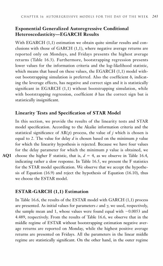
Exponential Generalized Autoregressive ConditionalHeteroscedasticity—EGARCH Results
With EGARCH (1,1) estimation we obtain quite similar results and con-clusions with those of GARCH (1,1), where negative average returns arereported only on Mondays, and Fridays presents the highest averagereturns (Table 16.3). Furthermore, bootstrapping regression presentslower values for the information criteria and the log-likelihood statistic,which means that based on these values, the EGARCH (1,1) model with-out bootstrapping simulation is preferred. Also the coefficient δ, indicat-ing the leverage effects, has negative and correct sign and it is statisticallysignificant in EGARCH (1,1) without bootstrapping simulation, whilewith bootstrapping regression, coefficient δ has the correct sign but is statistically insignificant.
Linearity Tests and Specification of STAR Model
In this section, we provide the results of the linearity tests and STARmodel specification. According to the Akaike information criteria and thestatistical significance of AR(p) process, the value of j which is chosen isequal to 2. The value for delay d is chosen based on the minimum p valuefor which the linearity hypothesis is rejected. Because we have four valuesfor the delay parameter for which the minimum p value is obtained, wechoose the higher F statistic, that is, d 4, as we observe in Table 16.4,indicating rather a slow response. In Table 16.5, we present the F statisticsfor the STAR model specification. We observe that we accept the hypothe-sis of Equation (16.9) and reject the hypothesis of Equation (16.10), thuswe choose the ESTAR model.
ESTAR-GARCH (1,1) Estimation
In Table 16.6, the results of the ESTAR model with GARCH (1,1) processare presented. As initial values for parameters c and γ, we used, respectively,the sample mean and 1, whose values were found equal with 0.0053 and4.489, respectively. From the results of Table 16.6, we observe that in themiddle regime of ESTAR without bootstrapping estimation negative aver-age returns are reported on Monday, while the highest positive averagereturns are presented on Fridays. All the parameters in the linear middleregime are statistically significant. On the other hand, in the outer regime
chapter 16 AUTOR EGR ESSIVE MODELS for the Day of the Week 243
AQ1

Table 16.3 EGARCH (1,1) Results for the Day-of-the-Week Effect
Panel A. Parameters
Models Mean Equation βMON βTUE βWED βTHU βFRI γ
0.00057 0.00017 0.00065 0.00037 0.00890 0.1062
[5.048]* [1.584] [5.688]* [3.216]* [7.433]* [13.121]*
EGARCH (1,1) Variance Equation ω α1 α2 δ
0.2061 0.1273 0.9888 0.0725
[13.97]* [17.871]* [781.48]* [15.38]*
Panel B. Diagnostics
R2adjusted AIC SBC LL LBQ2 (12) ARCH-LM (5) F statistic
0.000670 6.937 6.931 51497.25 30.788 5.609 11.554
(0.002) (0.000) (0.000)
Panel A. Parameters
EGARCH (1,1) Mean Equation βMON βTUE βWED βTHU βFRI γwith bootstrappingsimulation
0.00049 0.00015 0.00077 0.00032 0.000880 0.1042
[3.196]* [3.424]* [5.832]* [2.335] † [6.345]* [17.468]*
244
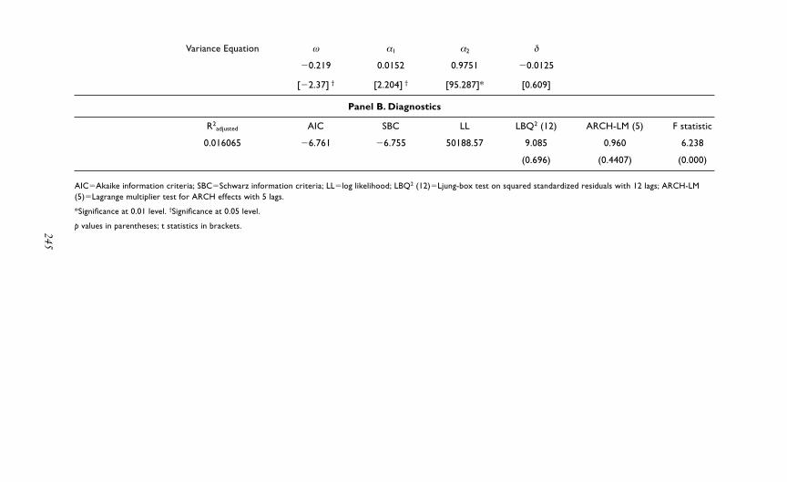
Variance Equation ω α1 α2 δ
0.219 0.0152 0.9751 0.0125
[2.37] † [2.204] † [95.287]* [0.609]
Panel B. Diagnostics
R2adjusted AIC SBC LL LBQ2 (12) ARCH-LM (5) F statistic
0.016065 6.761 6.755 50188.57 9.085 0.960 6.238
(0.696) (0.4407) (0.000)
AICAkaike information criteria; SBCSchwarz information criteria; LLlog likelihood; LBQ2 (12)Ljung-box test on squared standardized residuals with 12 lags; ARCH-LM(5)Lagrange multiplier test for ARCH effects with 5 lags.
*Significance at 0.01 level. †Significance at 0.05 level.
p values in parentheses; t statistics in brackets.245

with ESTAR estimation, significant positive average returns are presentedonly on Mondays, while negative returns are reported on Tuesdays. Thereturns of the other days of the trading week are statistically insignificant.The model corrects for autocorrelation and ARCH effects in all signifi-cance levels. Based on the F statistic, we reject the null hypothesis that theregression coefficients are equal.
In bootstrapping ESTAR estimation and the middle regime, we con-clude that there is the day-of-the-week effect, while the highest returnsare presented on Fridays and negative returns on Mondays. All the coeffi-cients in the middle regime are statistically significant. In the outerregime and the bootstrapping regression only, coefficients π21, βMON, andβWED are significant, and we observe that there is a reverse Monday effect,while the average returns on Mondays are positive and the averagereturns are negative on Wednesdays. The remaining weekday averagereturns are statistically insignificant. The bootstrapping ESTAR correctsfor both autocorrelation and ARCH effects. According to F statistic, thenull hypothesis of the coefficients equality is rejected. We observe thatbased on the information criteria and log-likelihood statistic, ESTARoutperforms the previous models, except from EGARCH, but the com-parison might not be the most appropriate as the formulation of the lastmodel is different.
246 Part i I I EXCHA NGE-TR ADED FUND STR ATEGIES
Table 16.4 Linearity Tests for S&P 500 Index
Delay (d) 1 2 3 4 5 6 7 8 9
F statistic 3.475 1.714 0.246 20.623 4.521 16.137 0.065 0.001 12.481
(0.002) (0.113) (0.960) (0.000) (0.000) (0.000) (0.998) (1.000) (0.000)
p values in parenthesis.
Table 16.5 STAR Model Specification for S&P 500 Index
F statistic H04 : F statistic H03 : F statistic H02 :Delay (d) β4 0 β3 0 / β4 0 β2 0 / β3 β4 0 Type of Model
4 0.0006 30.278 18.068
(0.9994) (0.000) (0.000) ESTAR
p values in parentheses
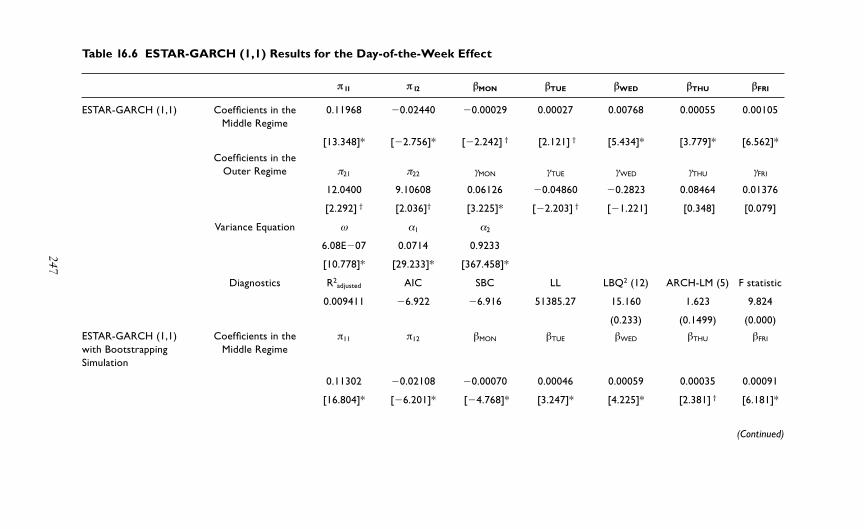
247
Table 16.6 ESTAR-GARCH (1,1) Results for the Day-of-the-Week Effect
π11 π12 βMON βTUE βWED βTHU βFRI
ESTAR-GARCH (1,1) Coefficients in the 0.11968 0.02440 0.00029 0.00027 0.00768 0.00055 0.00105Middle Regime
[13.348]* [2.756]* [2.242] † [2.121] † [5.434]* [3.779]* [6.562]*
Coefficients in the Outer Regime π21 π22 γMON γTUE γWED γTHU γFRI
12.0400 9.10608 0.06126 0.04860 0.2823 0.08464 0.01376
[2.292] † [2.036]† [3.225]* [2.203] † [1.221] [0.348] [0.079]
Variance Equation ω α1 α2
6.08E07 0.0714 0.9233
[10.778]* [29.233]* [367.458]*
Diagnostics R2adjusted AIC SBC LL LBQ2 (12) ARCH-LM (5) F statistic
0.009411 6.922 6.916 51385.27 15.160 1.623 9.824
(0.233) (0.1499) (0.000)
ESTAR-GARCH (1,1) Coefficients in the π11 π12 βMON βTUE βWED βTHU βFRI
with Bootstrapping Middle RegimeSimulation
0.11302 0.02108 0.00070 0.00046 0.00059 0.00035 0.00091
[16.804]* [6.201]* [4.768]* [3.247]* [4.225]* [2.381] † [6.181]*
(Continued)

Table 16.6 (Continued)
Coefficients in the π21 π22 γMON γTUE γWED γTHU γFRI
Outer Regime
7.39233 0.05273 0.01017 0.0137 0.0223 0.01715 0.12192
[1.785] ‡ [0.008] [1.803] ‡ [0.153] [2.77]* [0.127] [1.247]
Variance Equation ω α1 α2
2.83e05 0.0052 0.6758
[2.047]† [2.647]* [4.233]*
Diagnostics R2adjusted AIC SBC LL LBQ2 (12) ARCH-LM (5) F statistic
0.015165 6.755 6.746 50148.48 11.064 0.601 14.332
(0.523) (0.4369) (0.000)
AIC Akaike information criteria; SBC Schwarz information criteria; LL log likelihood; LBQ2 (12) Ljung-box test on squared standardized residuals with 12 lags; ARCH-LM (5) Lagrange multiplier test for ARCH effects with 5 lags.
*Significance at 0.01 level. †Significance at 0.05 level. ‡Significance at 0.10 level.
p values in parentheses; t statistics in brackets.
248

Forecasting Results and Performance
In Table 16.7, we report the forecasting performance measures. The meanabsolute error (MAE) is very close and the root mean square error (RMSE)is identical with all models, except in the ESTAR model, for in-sampleperiod, which the latter model presents the best performance. In out-of-sample period, RMSE and MAE are lower in GARCH (1,1), followed byOLS, and then by EGARCH (1,1). ESTAR-GARCH (1,1) presents lowerRMSE and MAE and so better forecasts performance. In the percentage ofthe correct signal criteria, OLS and EGARCH (1,1) model outperformGARCH (1,1), where the first two models capture the correct signal at56.7 percent (34 of 60) trading days, while GARCH (1,1) captures cor-rectly at 55.0 percent (33 of 60) trading days. ESTAR-GARCH (1,1) out-performs all models, capturing the correct signal in 38 of 60 trading daysor a percentage order of 63.4 percent. Specifically in the short horizon of10 ahead periods, ESTAR-GARCH (1,1) predicts correctly at 70 percent,while OLS predicts correctly at 60 percent and GARCH models capturethe correct signal only at 30 percent. In particular, many investors and trad-ers are interested in the forecasting of the correct signal over a five-daytrading week. For this purpose, ESTAR-GARCH model outperforms sig-nificantly the simple GARCH models.
CONCLUSION
In this chapter we examine the day-of-the-week effect on the S&P 500index. We find that this calendar anomaly exists according to all estima-tions, except in ESTAR-GARCH (1,1), where the Monday effect exists in
chapter 16 AUTOR EGR ESSIVE MODELS for the Day of the Week 249
Table 16.7 Forecasting Criteria for the Estimated Models
Percentage of Correct Signal inOut-of-Sample
Models In-Sample Out-of-Sample Period
RMSE MAE RMSE MAE
OLS 0.009316 0.006374 0.026476 0.020524 56.7%
GARCH (1,1) 0.009316 0.006376 0.026465 0.020493 55.0%
EGARCH (1,1) 0.009316 0.006375 0.026495 0.020552 56.7%
ESTAR-GARCH (1,1) 0.008729 0.006165 0.026248 0.020330 63.4%
the linear middle regime and the reverse Monday effect is reported in thenonlinear outer regime. We propose the STAR models for the day-of-the-week effect; however, this is only a proposed model, which was examinedfor only one calendar anomaly and using only one index, while furtherresearch can be applied in other calendar effects. Furthermore, the fore-casting performance of ESTAR model outperforms the forecasting abilityof the other estimated models, especially regarding the correct signal,which is the most important and realistic tool in real-world trading envi-ronments.
REFERENCES
Aggarwal, A. and Tandon, K. (1994) Anomalies or Illusions? Evidence fromStock Markets in Eighteen Countries. Journal of International Moneyand Finance, 13(1): 83–106.
Alagidede, P. (2008) Day of the Week Seasonality in African Stock Mar-kets. Applied Financial Economics Letters, 4(2): 115–120.
Alagidede, P. and Panagiotidis, T. (2009) Calendar Anomalies in the GhanaStock Exchange. Journal of Emerging Market Finance, 8(1): 1–23.
Aslanidis, N. (2002) Smooth Transition Regression Models in UK StockReturns. Working paper, University of Crete, Rethymno, Crete.
Bollerslev, T. (1986) Generalized Autoregressive Conditional Heteroscedas-ticity. Journal of Econometrics, 3(2): 307–327.
Chan, K.S. and Tong, H. (1986) On Estimating Thresholds in Autoregres-sive Models. Journal of Time Series Analysis, 7(3): 178–190.
Davidson, R. and MacKinnon, J.G. (2004) Econometric Theory and Methods.New York: Oxford University Press.
Draper, P. and Paudyal, K. (2002) Explaining Monday Returns. The Journalof Financial Research, 25(4): 507–520.
Engle, R. (1982) Autoregressive Conditional Heteroskedasticity With Esti-mates of the Variance of U.K. Inflation. Econometrica 50(4): 987–1008.
Hamilton, J.D. (1989) A New Approach to Economic Analysis of Nonsta-tionary Time Series and the Business Cycle. Econometrica, 57(1):357–384.
Kenourgios, D. and Samitas, A. (2008) The Day of the Week Effect Pat-terns on Stock Market Return and Volatility: Evidence for the Athens
250 Part i I I EXCHA NGE-TR ADED FUND STR ATEGIES

Stock Exchange. International Research Journal of Finance and Eco-nomics, 15(2):78–89.
Lakonishok, J. and Smidt, S. (1988) Are Seasonal Anomalies Real? ANinet y-Year Perspective. The Review of Financial Studies, 1(4):403–425.
McMillan, D.G. (2003) Non-linear Predictability of UK Stock MarketReturns. Oxford Bulletin of Economics and Statistics, 65(5): 557–573.
Mehdian, S. and Perry, M. (2001) The Reversal of the Monday Effect: NewEvidence from US Equity Markets. Journal of Business Finance andAccounting, 28(7/8): 1043–1065.
Mills, T.C., Siriopoulos, C., Markellos, R.N., and Harizanis, D. (2000)Seasonality in the Athens Stock Exchange. Applied Financial Economics,10(2):137–142.
Nelson, D.B. (1991) Conditional Heteroskedasticity in Asset Returns: ANew Approach. Econometrica, 59(2): 347–370.
Onyuma, S.O. (2009) Day-of-the-Week and Month-of-the-Year Effect onthe Kenyan Stock Market Returns. Eastern Africa Social ScienceResearch Review, 25(2): 53–74.
Pettengill, G.N. (2003) A Survey of the Monday Effect Literature. Quar-terly Journal of Business and Economics, 42(3/4): 3–28.
Teräsvirta, T. and Anderson, H.M. (1992) Characterizing Nonlinearities inBusiness Cycles using Smooth Transition Autoregressive Models. Jour-nal of Applied Econometrics, 7(2):119–136.
Teräsvirta, T., Lin, C.F., and Granger, C.W.J. (1993) Power of the NeuralNetwork Linearit y Test. Journal of Time Series Analysis, 14(2):209–220.
Teräsvirta, T. (1994) Specification, Estimation, and Evaluation of SmoothTransition Autoregressive Models. Journal of the American StatisticalAssociation, 89(425): 208–218.
Tong, H. (1990) Nonlinear Time Series: A Dynamical System Approach.Oxford, UK: Oxford University Press.
[AQ1]AQ: Sentence as rewritten ok for sense and intent of meaning?
chapter 16 AUTOR EGR ESSIVE MODELS for the Day of the Week 251

This page intentionally left blank

P A R T I V
FOREIGNEXCHANGEMARKETS,
ALGORITHMICTR ADING, AND RISK

This page intentionally left blank

255
17C H A P T E R
Disparity of USDInterbank InterestRates in Hong Kongand SingaporeIs There Any Arbitrage Opportunity?
Michael C. S. Wongand Wilson F. Chan
ABSTRACT
This chapter compares USD interest rates in two interbank markets,namely, Hong Kong Interbank Best Offer Rate (HIBOR) and SingaporeInterbank Best Offer Rate (SIBOR). Both Hong Kong and Singapore areglobal currency trading centers located in the same time zone, in whichthere are many global banks, fund houses, and hedge funds. However, wefind a consistent disparity between HIBOR and SIBOR in 2008, whicheven reaches 90 basis points after June 2008. This obviously contradicts thewell-known efficient market hypothesis. This chapter attempts to explainwhy bank dealers would be reluctant to do arbitrage.
INTRODUCTION
USD is an international currency for international transactions. Manyinternational activities on lending and borrowing are based on USD, under-gone in New York, London, Zurich, Singapore, Hong Kong, or Tokyo. The

interbank markets for USD funds should be very efficient because of thepresence of dealers from global banks. Disparity in the USD interest ratein these markets should be extremely narrow and directionless, especiallywhen the markets operate in the same time zone. This chapter comparesthe USD interbank fixing rate in Hong Kong and Singapore, denoted byHIBOR and SIBOR. We find that HIBOR is consistently higher thanSIBOR in 2008. The disparity becomes much wider after June 2008 andreaches to 80 basis points. This seems to be inconsistent with the well-known efficient market hypothesis (EMH) and to provide traders arbitrageopportunities.
Previous studies on interest rate and interest spreads document thatcredit risk, liquidity risk, and tax can affect interest rate (see, for instance,Elton et al. 2001; Eom Helwege, and Uno, 2003; and Longstaff, 2004).These studies focus mainly on the corporate bond market in the UnitedStates. Few studies explore the interest spreads in the interbank moneymarket. It is generally assumed that borrowers in interbank markets arecredible participants, spreads in interbank markets could be negligible, andtraders do not have any arbitrage opportunity. However, our evidenceshows a contradictory picture.
This chapter will proceed as follows: the second section of this chapterintroduces the HIBOR and SIBOR markets. This chapter’s third sectiondescribes our data and findings. The fourth section of this chapter providesexplanations on the disparity between HIBOR and SIBOR, and the fifthsection concludes the chapter.
HIBOR AND SIBOR
Interbank markets are very active in major international banking centers,such as New York, London, Singapore, and Hong Kong. Bank dealers bringglobal supply and demand to these markets in order to exchange for funds.They may also actively look for arbitrage opportunities. It would be veryhard to find any evidence of market inefficiency in interbank markets forthose actively traded products.
A USD fund is an actively traded product in interbank markets of differ-ent regions. Interest rate calculation for floating rate assets and liabilitiesdenominated in USD are mostly based on USD interbank rate plus aspread. Outside the United States, the interbank USD interest rate gener-ally refers to London Interbank Bank Offer Rate (LIBOR), Singapore
256 Part iV FOREIGN EXCHANGE MARKETS, ALGORITHMIC TR ADING, AND RISK

Interbank Offer Rate (SIBOR), and Hong Kong Interbank Offer Rate(HIBOR), respectively. Interbank dealers will collectively fix the interestrate in both the AM and PM. These are so-called AM and PM fixings. AMfixing is commonly used as a basis for interest rate calculation. In New Yorkthere is no New York interbank offer rate, although New York is an activemoney market. Both LIBOR and SIBOR have had a long history in themarket. The Hong Kong banking community formally launched the USDfixing rate on December 18, 2006. This is also the start of the sampleperiod of this study.
DATA AND FINDINGS
This chapter selects 1-month, 3-month, and 6-month USD interest ratesin the period between December 18, 2006 and November 28, 2008 foranalysis. The interest rates are interbank fixing rates (AM) in Hong Kongand Singapore (i.e., HIBOR and SIBOR). Figure 17.1 shows 3-monthHIBOR and SIBOR in the sample period. The two USD interest ratesmove closely and HIBOR tends to move higher than SIBOR in 2008. Figures 17.2 to 17.4 show the disparity between HIBOR and SIBOR for
chapter 17 DISPAR ITY OF USD INTERBA NK INTER EST R ATES 257
7.0000
6.0000
5.0000
4.0000
3.0000
2.0000
1.0000
HIBOR SIBOR
18/1
2/06
18/2
/07
18/4
/07
18/6
/07
18/8
/07
18/1
0/07
18/1
2/07
18/2
/08
18/4
/08
18/6
/08
18/8
/08
18/1
0/08
–
Figure 17.1 Three-Month USD HIBOR and SIBOR (in %): December 18,2006 to November 28, 2008

258 Part iV FOREIGN EXCHANGE MARKETS, ALGORITHMIC TR ADING, AND RISK
1.000
0.800
0.600
0.400
0.200
0.000
0.200
HIBOR-SIBOR(1m)
18/1
2/06
18/2
/07
18/4
/07
18/6
/07
18/8
/07
18/1
0/07
18/1
2/07
18/2
/08
18/4
/08
18/6
/08
18/8
/08
18/1
0/08
Figure 17.2 Difference between HIBOR and SIBOR: 1-Month Tenor
1.000
0.800
0.600
0.400
0.200
0.000
0.200
HIBOR-SIBOR(3m)
18/1
2/06
18/2
/07
18/4
/07
18/6
/07
18/8
/07
18/1
0/07
18/1
2/07
18/2
/08
18/4
/08
18/6
/08
18/8
/08
18/1
0/08
Figure 17.3 Difference between HIBOR and SIBOR: 3-Month Tenor

1-month, 3-month, and 6-month tenors, respectively. In Figure 17.2, 1-month HIBOR is consistently higher than 1-month SIBOR in 2008.The average difference is around 15 basis points in the period betweenJanuary 2008 and June 2008. The difference finally reaches 80 basis pointsin September and October of 2008. A similar phenomenon also happens to3-month and 6-month HIBOR and SIBOR.
EXPLANATIONS FOR THE HIBOR-SIBOR DISPARITY
According to logic of EMH, the disparity between HIBOR and SIBORshould be corrected quickly because both markets are trading the sameproduct and in the same time zone. One important assumption of EMH isthe presence of professional traders who are able to do arbitrage. Their col-lective efforts should effectively correct any mispricing. In the interbankmoney market, bank dealers take the role of the “professional traders” andare assumed to actively look for arbitrage opportunities. In practices, bankdealers have some constraints in their arbitrage decisions, including:
• Capital requirement: Basel II, the global banking regulation,requires capital requirements on credit exposures to other banks.
chapter 17 DISPAR ITY OF USD INTERBA NK INTER EST R ATES 259
0.600
0.500
0.300
0.400
0.200
0.100
0.000
0.100
HIBOR-SIBOR(6m)
18/1
2/06
18/2
/07
18/4
/07
18/6
/07
18/8
/07
18/1
0/07
18/1
2/07
18/2
/08
18/4
/08
18/6
/08
18/8
/08
18/1
0/08
Figure 17.4 Difference between HIBOR and SIBOR: 6-Month Tenor

Many banks have internal guidelines that bank dealers are not allowedto take unnecessary funds and credit positions. This restricts bankdealers from taking the benefit of arbitrage. Nonbank institutions donot have such constraints, but they cannot easily access the HIBORand SIBOR markets. If they want to make gains from arbitragebetween HIBOR and SIBOR, they will require a wider gap betweenHIBOR and SIBOR to compensate their transactions costs paid tobank dealers.
• Counterparty risk: In 2008, counterparty risk was a big issue ininterbank transactions. The financial troubles of Bear Stearns inMarch 2008 triggered off concerns over the financial soundness ofglobal institutions. Bank dealers became more sensitive to creditquality in lending via the interbank markets. The financial crisis thathappened in July to October in 2008 made bank dealers to beextremely cautious in allocating their credit exposures. The higherHIBOR against SIBOR might indicate higher credit risk involved inthe Hong Kong interbank market. This can be true as there is highernumber of small-sized banks in Hong Kong than in Singapore.
• Liquidity risk: In 2008 liquidity was a big issue for many banks.Financial markets became volatile and marketable assets suddenlyturned to be less marketable. To assure liquidity, banks would preferloans of much shorter maturity, such as overnight loans. Thisweakened the incentives of bank dealers to do arbitrage in the 1-month, 3-month, and 6-month interbank market.
CONCLUSION
The previous finding shows evidence of disparity between HIBOR andSIBOR, which are USD interbank fixing rates in Hong Kong and Singapore,respectively. The disparity stays at around 15 basis points in the first-half of2008 and even reaches 90 basis points in the crisis period of 2008. Eventhough the disparity provided bank dealers arbitrage opportunities, theymight find hard it to do arbitrage because of consideration on capitalrequirements, counterparty risk, and liquidity risk. Efficient market hypoth-esis might have overstated the power of professional traders. In volatile market environments, arbitrage opportunities may exist but professionaltraders could become reluctant to arbitrage.
260 Part iV FOREIGN EXCHANGE MARKETS, ALGORITHMIC TR ADING, AND RISK

REFERENCES
Elton, E., Gruber, M., Agrawal, D., and Mann, C. (2001) Explaining theRate Spread on Corporate Bonds. The Journal of Finance, 56(1):247–277.
Eom, Y.H., Helwege, J., and Uno, J. (2003) Structural Models of CorporateBond Pricing: An Empirical Analysis. Review of Financial Studies, 17(2):499–544.
Longstaff, F. (2004) The Flight-to-Liquidity Premium in U.S. TreasuryBond Prices. The Journal of Business, 77(3): 511–526.
chapter 17 DISPAR ITY OF USD INTERBA NK INTER EST R ATES 261

This page intentionally left blank

263
18C H A P T E R
Forex TradingOpportunitiesThrough PricesUnder ClimateChange
Jack Penm and R. D. Terrell
ABSTRACT
We have undertaken this research in forex trade assessment and investmentdecisions under climate change, using new and important zero-non-zeropatterned time-series approaches. Our results indicate that Granger feed-back relations exist in the system, involving exchange rates and priceindexes. This is valuable not only in predicting price changes but also incapturing forex trading opportunities.
INTRODUCTION
Powerful computing equipment has had a dramatic impact on forex model-ing and simulations, and has motivated development of innovative comput-ing-intensive time-series approaches to forex trade assessment for capturingtrading opportunities. New zero-non-zero (ZNZ) patterned time-seriesmethodology has specified models in a more sophisticated manner. This has

enabled the use of data in highly adaptive ways and facilitated major innova-tions in development of management and evaluation of forex modeling andtrading strategy. Against that background, we undertake research in forexmovement modeling and data analysis using new and important patternedtime-series approaches. While trade and environmental investment deci-sions still have to operate in an uncertain market, and human judgment cannever be fully replaced, quantitative time-series analysis has an importantrole to play in guiding effective trade decisions and setting trade strategy.
This chapter investigates a very important issue, namely, causal linksbetween exchange rates and price indexes, and undertakes an assessment ofthe causal positioning of the significant relevant economic variables involvedin the interactions. Perhaps the simplest of many contending hypotheses isthat there is a short-term causal link, in which international capital flowslead movements in the exchange rate. The absence of stable long-term rela-tionships would indicate that, over a long period, the levels of exchangerates are less dependent on the levels of prices. If stable long-term relation-ships exist among exchange rates and price indexes, then, after temporarydeviations in the short term, the levels of exchange rates would revert totheir traditional long-term relationships with price indexes. Identification ofsuch long-term relationships, if they exist, would be essential in forecastingexchange rate movements, which affects buying and selling trade behaviorand thereby identifies future trading opportunities.
We test this hypothesis using recent developments in cointegration the-ory. The tests are undertaken within the framework of ZNZ patternedvector error-correction modeling (VECM) and associated cointegratingvectors, with allowance for possible zero entries proposed in Penm andTerrell (2003). This approach is particularly useful for analyzing cointe-grating relationships between prices and exchange rates in forex trademarkets. Its special attraction is that, by permitting zero coefficients in theVECM, it allows for a highly insightful economic interpretation of thecointegrating relationships and their re-adjustment following deviationsfrom equilibrium. New error-correction technologies for linear and nonlinear modeling are helpful in explaining and interpreting certainaspects of causal links between prices and exchange rates. The patternedcointegrating vectors in the VECM are valuable not only in taking tradingopportunities but also in forecasting price changes.
There are also several other issues that must be addressed before we setout the full complexity of the pattern of linkages we are to investigate.
264 Part iV FOREIGN EXCHANGE MARKETS, ALGORITHMIC TR ADING, AND RISK

The relevant price variables may differ from country to country and at dif-ferent points in the sequence of events. We therefore examine consumerprices, wholesale prices, and export and import prices, in order to fullyunderstand the strength and direction of certain causal links. We also con-sider whether such links are short term or long term in nature and whetherit is possible in a complex sequential process to detect feedback loops. Weconstruct a system model to investigate the following two causal chains.
chapter 18 FOREX TR ADING OPPORTUNITIES Under Climate Change 265
1. c.i. e.r
2. c.i. e.r
m
e.a.
e.a.
m
c.p.
w.p. pdy
e.r.
pdy
e.r.
e.p.
e.p.
m.p.
m.p.
c.p.
w.p.
We also propose to include a forgetting factor in the estimation of thepatterned VECMs. The forgetting factor technique is a data-weightingprocess that allows the estimation to place greater weight on more recentobservations and less weight on earlier data. In such estimation, the effectson the underlying relationships of evolution generated by the causal linkageprocess will be accounted for.
As to why a subset time-series model is used, subset modeling includesfull-order models, and researchers use this approach whenever measure-ments exhibit some periodicity. If the underlying true time-series processhas a subset structure, the suboptimal full-order specification can giverise to inefficient estimates and inferior projections. Our forgetting factorapproaches improve estimated parameter profile, model structure, andperformance reliability for assessing complex relationships involving
c.i. capital flows: e.r. exchange rates: m money supply movements; e.a. economic activities; c.p. consumer prices; w.p. whole prices: e.p. exportprices: m.p. import prices: pdy productivity changes.

slowly evolving long-term effects, such as climate change. These qualitiesare not found in conventional time-series approaches involving only full-order models. Subset modeling is superior to full-order modeling for dis-covering complex relationships, as has been clearly indicated in Penm andTerrell (2003).
In order to illustrate the practical use of the proposed forex modelingand trade forecast approach, we investigate the causal relationships amongexchange rates, price indexes, other macroeconomic variables, and theexchange rate forecasting in Taiwan using the monthly data over the period1982 to 2008. Researchers have recognized the potential hazards that cli-mate change and environmental change may present for small island devel-oping states such as Taiwan. Changes are expected to be negativelyimpacted, and thus directly threaten the Taiwanese population. Thosechanges include: a general rise in surface temperature and in sea level;changes in seasonal temperature variation and rainfall patterns; variations insoil moisture and water resources; and increases in the incidence of severeweather events such as typhoons and floods.
Climate change in Taiwan has both environmental and socioeconomicoutcomes for agriculture: changes in the availability and quality of land,soil, and water resources, for example, may later be reflected in poorer cropperformance, which causes prices to rise. Climate-related changes in agri-cultural conditions will likely only increase Taiwan’s dependence onimported food. The price indexes track changes in the prices consumerspay for products and services. Those price indexes will therefore trackchanges over time in the long-term effects of climate changes and theirimpacts on the production, use, and disposal of items purchased each yearby consumers.
This chapter is organized as follows: the second section of this chapteroutlines the construction of patterned vector error-correction modeling,which demonstrates the “presence and absence” restrictions on the coeffi-cients of subset time-series systems, including full-order systems. Also, briefdescriptions are given of the forgetting factor techniques used for estima-tion. In this chapter’s third section we assess the causal link betweenexchange rates and price indexes in Taiwan. We also present the forex forecasting results indicating significant movements in exchange rates, inwhich the MAE criterion is used to examine prediction performance. A briefsummary is provided in the final section of this chapter.
266 Part iV FOREIGN EXCHANGE MARKETS, ALGORITHMIC TR ADING, AND RISK

METHODOLOGY
The Forgetting Factor
The use of forgetting factor in time-series analysis has attracted consider-able interest in recent years. For example, Penm and Terrell (2003) utilize aforgetting factor in subset autoregressive modeling of the spot aluminumand nickel prices on the London Metal Exchange. The use of the forgettingfactor technique to estimation and simulation of financial market variableshas been reported by Brailsford, Penm, and Terrell (2002).
Consider a vector autoregression (VAR) model of the following form:
(18.1)
y(t) is a sx1 vector of wide-sense stationary series. ε(t) is a sx1 vector ofindependent and identically distributed random process with Eε(t) 0 andEε(t)ε′(t τ) V if τ 0 and 0 if τ 0. Bτ, τ 1, …, q are sxs matricesof coefficients. The observations y(t) t 1, … , T are available.
Let λ(t) [λ1(t) … … λn (t)] denotes a 1xs vector associated with time t.Following O’Neill, Penm, and Penm (2007), a strategy for determining thevalue of the forgetting factor λ(t) is as follows:
(18.2)
Equation (18.2) means that “forgetting” of the past occurs from time η.No forgetting is involved from time η 1 to time T. If λ 1 for every t,then we obtain the ordinary least squares solution. If 0 λ 1, the past isweighted down geometrically from time η. In theory, the value of λ couldbe different between λi(t) (a so-called variable forgetting factor). For sim-plicity, we only consider the fixed forgetting factor case in which the valueof λ is constant for λi(t).
This means that the coefficients in Equation (18.1) are estimated tominimize
(18.3)
chapter 18 FOREX TR ADING OPPORTUNITIES Under Climate Change 267
y t B y t tq
( ) ( ) ( )+ − ==
∑ ττ
τ ε1
λ λ η ηηi
tt t t T i( ) ,= ≤ ≤ = < ≤ =− +1 1 1if and 1 if for …nn
λ τ ττ τττ
( )[ ( ][ ]t y t B y t y t B y tqq
( ) ) ( ) ( )− − − −==
∑11
∑∑∑=t
T
1
′

One important issue relating to the use of the forgetting factor in estima-tion is how to determine the value of λ in applications. The conventionalmethod is based on arbitrary or personal choices. Penm and Terrell (2003)propose to determine the value of λ using bootstrapping. In this study, theirrecommended method is adopted for the determination of the value of λ. While Brailsford, Penm, and Terrell (2002) also propose a procedure todetermine the value of dynamic forgetting factor for nonstationary systems,we have focused on the use of a fixed forgetting factor in this study, becauseapplications of a fixed forgetting factor to forex market movements is likely tobe more predictable.
VECM Modeling for an I(1) System
In constructing V ECM modeling for an I(1) system, from Equation(18.1) we have Bq(L) I Σ
q
τ1BτLτ, where L denotes the lag operator, and
Ly(t) y(t1). It is assumed that the roots of |Bq(L)| 0 lie outside oron the unit circle to ensure that y(t) can contain I(1) variables.
Of note, y(t) is integrated of order d, I(d), if it contains at least one element which must be differenced d times before it becomes I(0). Further,y(t) is cointegrated with the cointegrating vector, β, of order g, if β’y(t) is integrated of order (d – g), where y(t) has to contain at least two I(d) variables.
Following Penm and Terrell (2003), the equivalent VECM for Equation(18.1) can then be expressed as
Bq(1)y(t 1) Bq–1 (L)y (t) ε(t) (18.4)
where y(t) contains variables of the types I(0) and I(1). Note that (IL),y(t) y(t) y(t1) and ε(t) is stationary. Equation (18.4) can be rewritten as
B*y(t 1) Bq1(L)y(t) ε(t), (18.5)
where B* Bq (1) and B*y(t 1) is stationary and the first term in Equation(18.5) is the error-correction term. The term Bq–1 (L)y (t) is the vectorautoregressive part of the VECM.
268 Part iV FOREIGN EXCHANGE MARKETS, ALGORITHMIC TR ADING, AND RISK

Because y(t) is cointegrated of order 1, the long-term impact matrix, B*,must be singular. As a result, B* αβ′ and β′y(t 1) is stationary, wherethe rank of B* is r (0 r s), and α and β are matrices of dimensions s rand r 2s respectively. The columns of β are the cointegrating vectors andthe rows of are the loading vectors.
A search algorithm proposed by Penm and Terrell (2003) to select theoptimal ZNZ patterned α and β is described in the following:
1. To begin this algorithm we first identify the optimal ZNZ–patternedVECM, using model selection criteria.
2. After the optimal ZNZ–patterned VECM is identified, the rank ofthe long-term impact matrix is then computed using the singularvalue decomposition method so the number of cointegrating vectorsin the system will be known.
3. A tree-pruning algorithm which avoids evaluating all candidates isthen implemented for the search of all acceptable ZNZ patterns ofthe loading and cointegrating vectors.
4. The identified candidates of the ZNZ–patterned cointegratingvectors are estimated by the method based on a triangular ECMrepresentation proposed in Penm and Terrell (2003).
5. The estimation of the associated candidates for the ZNZ–patternedloading vectors is carried out by the regression method with linearrestrictions.
6. The optimal ZNZ patterned α and β are finally selected by modelselection criteria.
Model development is more convenient using VECMs, rather than theequivalent VARs, if the systems under study include integrated time-series.Penm and Terrell (2003) note that, for I(1) systems, the VARs in first dif-ference will be misspecified and the VARs in levels will ignore importantconstraints on the coefficient matrices. Although these constraints may besatisfied asymptotically, efficiency gains and improvements in forecasts arelikely to result by imposing them. The analogous conclusion applies to I(1)systems, such as those typically encountered in tests of purchasing powerparity. Comparisons of forecasting performance of the VECMs versusVARs for cointegrated systems have been reported in studies such as Penm
chapter 18 FOREX TR ADING OPPORTUNITIES Under Climate Change 269

and Terrell (2003). The results of these studies indicate that, while in theshort run there may be gains in using unrestricted VAR models, theVECMs produce long-run forecasts with smaller errors when the variablesused in the models satisfy the test for cointegration.
Further to these developments, we consider a hypothesis where every(i,j)-th element, for specified i and j, is zero in all coefficient matrices in aVAR. If this hypothesis is framed in the VAR expressed by Equation (18.1),these zero entries will also hold in the error-correction terms and in the vector autoregressive part of the equivalent VECM, say Equation (18.4). Adiscussion of this property is provided by Penm and Terrell (2003). Analo-gously, we can achieve a result that if all (i,j)-th coefficient elements in theerror-correction terms and all (i, j)-th coefficient elements in the vectorautoregressive part of the VECM are zeros, then every (i,j)-th entry is zerofor all coefficient matrices in a VAR. The implications of the above outcomeare straightforward. If yj does not Granger-cause yi, then any (i, j)-th entrymust be zero for all coefficient matrices in the VAR. Also all (i, j)-th coeffi-cient elements in the equivalent VECM are zeros.
In a similar way, we can demonstrate that if yj does Granger-cause yi , thenthe (i,j)-th element of Bq(L) in (1) is nonzero. Also, at least a single (i,j)-thecoefficient element is nonzero in Bq(1) or Bq–1(L) in the equivalent VECM.Of note, an indirect causality from yj to yi through ym indicates yj causing yi
but only through ym. Hence, yj Granger-causes ym, ym Granger-causes yi, andyj does not Granger-cause yi directly. We can easily demonstrate that theVAR in (18.2) has nonzero (m,j )-th and (i, m)-th elements and a zero (i, j)-thelement in Bq(L). This indirect causality can also be shown in the equivalentVECM, which has at least a single nonzero (m,j)-th element and a singlenonzero (i,m)-th elements in Bq(1) and Bq–1(L). Also all the (i, j)-th elementsin the equivalent VECM are zeros.
The previous discussion indicates that Granger causality, Granger non-causality, and indirect causality detected from both the ZNZ–patternedVECM and its equivalent ZNZ–patterned VAR are identical. Since the useof the VECM is more convenient, it is obvious the ZNZ–patterned VECMis a more straightforward and effective means of testing for the Granger-causal relations. The same benefits will be present if the ZNZ–patternedVECM is used to analyze cointegrating relations.
Cointegration theory is associated with “error-correction” and has impor-tant implications for forecasting. If cointegration is found to exist among cer-tain variables, then such long-term relationships should be explicitly identified
270 Part iV FOREIGN EXCHANGE MARKETS, ALGORITHMIC TR ADING, AND RISK

when forecasting, which is very important in capturing trading opportunityand setting trading strategies. Recent empirical studies have demonstratedthat imposing such restrictions in forecasting would significantly benefit theforecasts, especially in the longer term. Further, the development course ofthe climate change is a long-term slowly evolving underlying process, and the effects of climate change will be exhibited in the long-term patternedcointegrating relations, which are detected in the error-correction term ofthe patterned VECM.
DATA AND EMPIRICAL APPLICATION
In this study, monthly observations of economic price indexes and exchangerate variables over the period January 1982 to June 2008 are used (T 306).These data are obtained from the Taiwanese Economic Database. The year2000 is selected as the base year for all indexes involved. Table 18.1 presentsthose variables which are examined contemporaneously in a stochastic vectorsystem.
All variables, excluding BOPCF, are log transformed such that y1(t)
log(E), y2(t) BOPCF, y3(t) log(UCP), y4(t) log(UWP), y5(t)
log(UMP), y6(t) log(UXP), y7(t) log(UM2), y8(t) log(UEA), and y9(t) log(UPDY), Unit root tests indicate that all transformed series are I(1).Following Brailsford, Penm, and Terrell (2002), we apply a fixed forgettingfactor with the value 0.99 to the stochastic system involved. We then con-duct the search procedures proposed in Penm and Terrell (2003) to obtainthe optimal ZNZ–patterned VECM model over the period January 1982 toMarch 2007 (T 291).
chapter 18 FOREX TR ADING OPPORTUNITIES Under Climate Change 271
Table 18.1 Brief Description of Economic Variables Involved in a StochasticVector System
Variable Brief Description
USD Exchange rate (E): Taiwanese Dollar per U.S. Dollar
BOPCF Taiwanese capital inflow
UCP Ratio of price levels (P ): Taiwanese CPI relative to U.S. CPI
UWP Taiwanese WPI relative to U.S. WPI
UMP Taiwanese import price index relative to U.S. import price index
UXP Taiwanese export price index relative to U.S. export price index
UM2 Taiwanese M2 relative to US M2
UPDY Taiwanese industry production index relative to U.S. industry production index

In the course of selecting the optimal lag order (p) for the autoregres-sive part of the VECM system, we adopt the principle used by Penm andTerrell (2003) to enhance the procedure. That is, we examine whiteness forthe residual vectors from the VECM chosen by the Akaike informationcriterion. If the residual vector process proves to be nonwhite, we sequen-tially increase q to q 1, and check the resultant residual vector processuntil the process is a vector white noise process. An optimal value of 5 hasbeen identified for q, as the resultant residual vector process for q 5becomes a white noise process. The optimal ZNZ–patterned VECM withthe lags 1, 3, and 5 for the autoregressive part, and the optimal and arethen selected by using the modified Hannan-Quinn criterion (MHQC).Subsequently, we will use MHQC as an abbreviation for the modified cri-terion, which is defined by MHQC log |V| [2 log log f(T)/f(T)]N,where f(T) Σ
T
t1λT-t is the effective sample size, N is the number of func-
tionally independent parameters, and V is the sample estimate of V.Following the procedure for examining causality in Penm and Terrell
(2003), the selected VECM supports the two Granger causality chainswhich are shown below in Figure 18.1.
272 Part iV FOREIGN EXCHANGE MARKETS, ALGORITHMIC TR ADING, AND RISK
BOPCF
UCP
UWP
UMP
UXP
USD
UEA
UCP
UM3
UWP
UXPUPDY
UCP
UXP
USD
UPDY
USD
USD
UEA
UCP
UM 3
UWP
UXPUPDY
UCP
UXP
USD
UPDY
USD
Figure 18.1 Two Causal Chains Detected in VECM Modeling

We then utilize the model specification selection approach to select theoptimal patterned VECM models at T 292, 293, and 294. An identicalVECM specification with the lags 1, 3, and 5 for the autoregressive part isselected by the MHQC at all times. Further, the Taiwanese dollar to USDequation specified in the VECM modeling at T 294 is presented inTable 18.2. The t statistics are shown in brackets.
We then undertake the one-step ahead forecasts over the period July 2007to June 2008. The forecasts and the actual values are shown in Figure 18.2.
The value of MAE 3.3 percent over the period July 2007 to June 2008,
where .MAEforecast – actual value
actual valueii
= ∑
chapter 18 FOREX TR ADING OPPORTUNITIES Under Climate Change 273
M7 2007 M8 2007 M9 2007 M10 2007M11 2007M12 2007 M1 2008 M2 2008 M3 2008 M4 2008 M5 2008 M6 2008
34
33.5
32.5
31.5
US
D
Actual Forecasts
33
32
31
Figure 18.2 Forecast Values Against the Actual Values
Table 18.2 The Exchange Rate Equation Specified in VECM
DUSD 0.31588 DUSDt1 0.13877 ErrorCorrectiont1
(1.78) (3.32)
ErrorCorrectiont1 .27601USDt1 1.17940UWPt1 0.01314UCPt1 4.75997UMPt1
(2.58) (1.97) (3.82) (3.11)
8.83*106 BOPCFt1
(2.95)

CONCLUSION
The chapter presents the causal links between exchange rates and macro-economic price indexes, supported by patterned VECM modeling and sim-ulations with the forgetting factor in a relevant and complex forex tradeenvironment.
This approach can be used to guide further appropriate use of data in mon-itoring changes in forex trade environments. Methodologies and technologiescurrently used to analyze exchange rate, banking, and policy studies will haveaccess to a more rigorous academic methodology for handling databases builtup over periods of considerable structural change, resulting in improved andmore timely responses in their fields.
As the development course of climate change is a long-term, slowly evolv-ing, underlying process, the trading effects of climate change are exhibitedin the long-term patterned cointegrating relations, which are detected in theerror-correction term of the patterned VECM.
REFERENCES
Brailsford, T., Penm, J., and Terrell, R.D. (2002) Selecting the ForgettingFactor in Subset Autoregressive Modelling. Journal of Time SeriesAnalysis, 23(6): 629–650.
Mathematics and Decision Sciences, Article ID 46592: 1–12.
O’Neill, T., Penm, J., and Penm, J.S. (2007) A Subset Polynomial NeuralNetworks Approach for Breast Cancer Diagnosis. International Journalof Electronic Healthcare, 3(3): 293–302.
Penm, J. and Terrell, R.D. (2003) Collaborative Research in QuantitativeFinance and Economics. Australian Capital Territory, Australia: EvergreenPublishing.
274 Part iV FOREIGN EXCHANGE MARKETS, ALGORITHMIC TR ADING, AND RISK

275
19C H A P T E R
The Impact ofAlgorithmicTrading Models on the StockMarket
Ohaness G. Paskelian
ABSTRACT
The manner in which electronic trading is conducted on international finan-cial markets has dramatically changed in recent decades as more and morestages of the trading process have been radically altered by electronic means.One of the most recent developments is algorithmic trading which primarilyfocuses on the minimization of implicit transaction costs in order execution.Algorithmic trading models typically strive toward achieving or beating aspecified benchmark with their executions. An algorithmic trading modelcan be distinguished by its underlying benchmark, trading style, or aggres-siveness (Kissell and Malamut, 2006). The existing literature addressing theconcept of algorithmic trading focuses on the investors’ perspective. Thisresearch investigates algorithmic trading from a market perspective and its

impact on the market outcome. It emphasizes how the algorithmic tradingsystems can provide better trade execution and lower market volatility whencompared with traditional trading techniques.
INTRODUCTION
During the last decade, automation and new technologies have changed thelandscape of traditional trading systems. Algorithmic trading is one of themost widely used computerized automated systems and is very popularamong traders and investors. The basic concept of algorithmic trading is toslice an order in such a manner that its impact on the market will be minimal.Using mathematical models and real-time market data, algorithms can deter-mine both the optimum size of the order and its time of submission to themarket. This minimizes the impact of the order on the market. The volumeof trades using algorithmic trading models has been steadily increasing overthe past few years. In 2008 more than 40 percent of the transactions carriedon Deutsche Börse’s Xetra trading system were performed using algorithmictrading systems. According to Greenwich Associates, “the proportion ofUS equity trading volume executed electronically increased to 36 per cent in 2008–2009 from 32 per cent in 2007–2008—a shift attributable in largepart to the pick-up in algorithmic trading.” (Greenwich Associates, 2009).Greenwich Associates report that more than three-quarters of all U.S. insti-tutions and 95 percent of the largest and most active institutional traders usealgorithmic trading strategies. This accounts for approximately 18 percent ofoverall U.S. equity trading volume.
In the financial markets, orders forwarded to brokers-dealers can beeither discretionary or nondiscretionary. Nondiscretionary orders are to be executed immediately in a given market. Discretionary orders allow thebroker-dealer to decide on the quantities, timing, and method of execu-tion. Algorithmic trading systems are computerized models dealing withnondiscretionary orders without intervention from a human broker-dealer.Algorithms are designed to work discretionary orders within the realitiesof the market microstructure for securities (Baker and Tiwari, 2004).Algorithmic trading systems are particularly well suited for highly liquidsecurities traded on electronic limit order books. Since trading volume andprice-spread vary continuously over time, algorithms can be designed totrack a particular price or volume. Thus, a trading order can be executed
276 Part iV FOREIGN EXCHANGE MARKETS, ALGORITHMIC TR ADING, AND RISK
only within parameters specified by the algorithm to minimize its impacton the overall market.
In this chapter, we present an overview of the impact of algorithmictrading systems on market price, liquidity, and movement. We also providea description of the major strategies used in algorithmic trading systems.We conclude with a note on some future developments in this area.
THE IMPACT OF ALGORITHMIC TRADING ON THE MARKET
Algorithmic trading research is in its beginning stage. The following is asummary of the more prominent articles on this subject. Almgren andLorenz (2007) provide an overview of the evolution of algorithmic trad-ing systems over time. The first generation of algorithmic strategies aimsto meet benchmarks generated by the market itself. The benchmarks arelargely independent from the actual securities order. Examples of thisstrategy are the volume-weighted average price (VWAP) or an average ofdaily open-high-low-close (OHLC) prices. The second generation ofalgorithmic trading strategies aims to meet order-centric benchmarksgenerated at the time of order submission to the algorithm. The executionstrategy targets the minimization of the implementation shortfall, i.e., thedifference between decision price and final execution price. Second-gen-eration algorithms implement static execution strategies, which predeter-mine (before the start of the actual order execution) how to handle thetrade-off between minimizing market impact costs (by trading slowly)and minimizing the variance of the execution price (by trading immedi-ately) (Gsell, 2007). Third-generation algorithms implement dynamicexecution strategies which reevaluate strategy at each single decision time.This enables the model to respond to market developments dynamically.Trading aggressiveness can be altered during the course of the decisionmaking process (Almgren and Lorenz, 2007).
Yang and Jiu (2006) propose a framework to help investors to choose themost suitable algorithm. Morris and Kantor-Hendrick (2005) note somefactors that investors take into consideration when deciding to use an algo-rithmic trading system. Trading style and frequency, regulatory obligations,and trader experience were found to be significant variables when selectingan algorithmic trading system.
chapter 19 THE IMPACT OF ALGOR ITHMIC TR ADING MODELS 277

The literature provides studies covering the impact of algorithmic trad-ing models on different markets. Konishi (2002) proposes an optimal slicingstrategy for VWAP trades. Domowitz and Yegerman (2005) examine theexecution quality of algorithms in comparison with brokers’ traditionalmethod of handling large orders. They conclude that VWAP algorithms onaverage have an underperformance of 2 bps. This is counterbalanced by thefact that algorithms can be offered at lower fees than human order han-dling. Kissel (2007) outlines statistical methods to compare the perfor-mance of algorithmic trading solutions. Hendershott, Jones, and Menkveld(2007) present evidence that algorithmic trading and liquidity are positivelyrelated.
Chaboud et al. (2009) study the effects of algorithmic trading on theforeign exchange (FX) markets using three widely traded currency pairs.They find that algorithmic trading systems are not related to volatility andthat the variance in FX returns is not related to algorithmic trading orderflow. The authors suggest that there is a relationship between trade-corre-lated and trade-uncorrelated information processing patterns when compar-ing algorithmic trading systems and human traders. They conclude thatalgorithmic trading systems provide better quotes due to their ability toprocess more public information than a human trader.
Hendershott and Riordan (2009) provide a continuation of the previousstudy of Chaboud et al. (2009). They test the average level of algorithmictrading and human information (measured as the variance of the random-walk component of returns) and conclude that algorithmic trading ordersand quotes are more informative than are those made by humans. Riordanand Storkenmaier (2009) study the impact of the upgrade of DeutscheBörse electronic trading system on the information content of algorithmictrading systems. They find that the upgrade of the trading system hasdecreased trading costs and increased overall liquidity. Further, tradersusing algorithmic trading systems process information much faster thantheir human counterparts and thus increase the liquidity of the market andthe information content of the prices.
Finally, Gsell (2007) provides a simulation result of the implementationof algorithmic trading systems. He finds that algorithmic trading systemshave an impact on market outcome in terms of market prices and marketvolatility. He also finds that the low latency of the algorithmic systems hasthe potential to significantly lower market volatility. However, when he
278 Part iV FOREIGN EXCHANGE MARKETS, ALGORITHMIC TR ADING, AND RISK
simulated trading with larger volumes, the algorithmic trading systemresulted in negative market prices.
ALGORITHMIC STRATEGIES
One of the first algorithmic trading strategies consisted of using a volume-weighted average price, as the price at which orders would be executed. TheVWAP introduced by Berkowitz et al. (1988) can be calculated as the dollaramount traded for every transaction (price times shares traded) divided bythe total shares traded for a given period. If the price of a buy order islower than the VWAP, the trade is executed; if the price is higher, then thetrade is not executed. Participants wishing to lower the market impact oftheir trades stress the importance of market volume. Market volume impactcan be measured through comparing the execution price of an order to abenchmark. The VWAP benchmark is the sum of every transaction pricepaid, weighted by its volume. VWAP strategies allow the order to dilute theimpact of orders through the day. Most institutional trading occurs in fill-ing orders that exceed the daily volume. When large numbers of sharesmust be traded, liquidity concerns can affect price goals. For this reason,some firms offer multiday VWAP strategies to respond to customers’requests. In order to further reduce the market impact of large orders, cus-tomers can specify their own volume participation by limiting the volumeof their orders to coincide with low expected volume days. Each order issliced into several days’ orders and then sent to a VWAP engine for thecorresponding days. VWAP strategies fall into three categories: sell orderto a broker-dealer who guarantees VWAP; cross the order at a future dateat VWAP; or trade the order with the goal of achieving a price of VWAPor better (Madhavan, 2000).
The second algorithmic trading strategy is the time-weighted averageprice (TWAP). TWAP allows traders to slice a trade over a certain periodof time, thus an order can be cut into several equal parts and be tradedthroughout the time period specified by the order. TWAP is used fororders which are not dependent on volume. TWAP can overcome obstaclessuch as fulfilling orders in illiquid stocks with unpredictable volume. Con-versely, high-volume traders can also use TWAP to execute their ordersover a specific time by slicing the order into several parts so that the impactof the execution does not significantly distort the market.
chapter 19 THE IMPACT OF ALGOR ITHMIC TR ADING MODELS 279

Another type of algorithmic trading strategy is the implementationshortfall or the arrival price. The implementation shortfall is defined asthe difference in return between a theoretical portfolio and an imple-mented portfolio. When deciding to buy or sell stocks during portfolioconstruction, a portfolio manager looks at the prevailing prices (decisionprices). However, several factors can cause execution prices to be differentfrom decision prices. This results in returns that differ from the portfoliomanager’s expectations (Perold, 1988). Implementation shortfall is meas-ured as the difference between the dollar return of a paper portfolio(paper return) where all shares are assumed to transact at the prevailingmarket prices at the time of the investment decision and the actual dollarreturn of the portfolio (real portfolio return). The main advantage of theimplementation shortfall-based algorithmic system is to manage transac-tions costs (most notably market impact and timing risk) over the speci-fied trading horizon while adapting to changing market conditions andprices (Kissell and Malamut, 2006).
The participation algorithm or volume participation algorithm is used totrade up to the order quantity using a rate of execution that is in proportionto the actual volume trading in the market. It is ideal for trading largeorders in liquid instruments where controlling market impact is a priority.The participation algorithm is similar to the VWAP except that a tradercan set the volume to a constant percentage of total volume of a givenorder. This algorithm can represent a method of minimizing supply anddemand imbalances (Kim, 2007).
Smart order routing (SOR) algorithms allow a single order to exist simulta-neously in multiple markets. They are critical for algorithmic execution mod-els. It is highly desirable for algorithmic systems to have the ability to connectdifferent markets in a manner that permits trades to flow quickly and effi-ciently from market to market. Smart routing algorithms provide full integra-tion of information among all the participants in the different markets wherethe trades are routed. SOR algorithms are critical to the smooth operation of the highly fragmented U.S. market structure. In the United States alone,there are more than 100 trading venues on different electronic communica-tions networks (ECNs). Thus, SOR algorithms allow traders to place largeblocks of shares in the order book without fear of sending out a signal to othermarket participants. The algorithm matches limit orders and executes them atthe midpoint of the bid-ask price quoted in different exchanges.
280 Part iV FOREIGN EXCHANGE MARKETS, ALGORITHMIC TR ADING, AND RISK

ALGORITHMIC TRADING ADVANTAGES
Algorithmic trading systems provide a number of advantages over tradi-tional methods, including:
1. Increased capacity: Computerized algorithms have much morepowerful computational capabilities to handle computationallyintensive processes.
2. Decreased costs: Commissions for electronic trading tend to besignificantly lower than other types of trades.
3. Real-time feedback and control: Algorithmic trading provides betterfeedback mechanisms than traditional trading methods. The abilityof the algorithmic models to process new information is found to besuperior to that of the human trader.
4. Anonymity: Algorithmic trading provides privacy and anonymity byallowing the order originator to remain unknown. Also, since orderscan go through several brokers, the original time of the order canremain confidential .
5. Control of information leakage: Algorithmic trading protects tradersby preventing them from disseminating their alpha expectations toother market participants.
6. Access to multiple trading markets: Algorithms decideinstantaneously where to send the orders depending on the bestavailable market. Thus, orders can be placed on the best availablemarket crossing networks and internal flow.
7. Consistent execution methodology: Consistent execution was oneof the key factors behind benchmarks such as VWAP. Theknowledge of the algorithm enables the trader to understand howand why the algorithmic systems reacted to the market in anygiven situation.
8. Best execution and transaction-cost-analysis (TCA) real-time: TCA,including execution, impact, slippage, and correlation information,can be available instantaneously. Thus, analyzing all types of pre- andpost-trade scenarios can be performed.
9. Minimization of errors: The absence of human operators makesalgorithmic trading systems less prone to errors.
chapter 19 THE IMPACT OF ALGOR ITHMIC TR ADING MODELS 281

10. Compliance monitoring: Compliance rules including limits,exposure, and short sales can be validated in real-time, and alertscan be issued for any potential scenario.
ALGORITHMIC TRADING BEYOND STOCK MARKETS
Algorithmic trading is also spreading to other asset categories, includingforeign exchange, fixed income, futures, options, and derivatives. Thistrend is driven by the desire for competitive advantage combined withthe growing availability of electronic trade execution, third-party trad-ing networks, and robust order management systems. As with the equitysector, the most liquid instruments are receiving the initial focus whilemost others still require traditional trading techniques. The foreign-exchange market has long depended on phone brokerage with large banksand FX dealers. However, FX ECNs are taking the market forward byproviding the services and technology solutions which meet this need forgrowth and diversity. This in turn adds liquidity to the market as a widerrange of players is enabled to participate. Active traders have become anincreasingly important part of the global FX market in recent years.They have begun to treat FX as an asset class in its own right. Activetraders have found they can successfully employ the same algorithmictrading methods in FX to generate alpha as they have previously appliedto equity markets.
Slowly, these different trading venues are opening up and electronictrading can be executed in limited form. Like the futures market, which hasboth electronically traded and pit-traded contracts, the effectiveness ofalgorithmic trading will depend on the degree of electronic sophisticationin the market place. The prospect of multi-asset algorithmic trading modelsremains quite intriguing.
CONCLUSION
Algorithmic trading systems are designed to lower transaction costs, reducemarket impact, and create liquidity. A large trade executed through an algo-rithm should be efficient, while creating liquidity and avoiding risk in the
282 Part iV FOREIGN EXCHANGE MARKETS, ALGORITHMIC TR ADING, AND RISK

event the market turns in the opposite direction. Another advantage of thealgorithmic trading systems is the splicing and execution of multiple smallorders from a big order, thus minimizing market impact. Simultaneously,the ability of the algorithmic trading systems to monitor and provide real-time feedback ameliorates the chances of the best execution of these orders.Moreover, a large order using a number of different algorithms to accessdifferent markets simultaneously can result in faster and quicker executionof the order.
However, as the market share of algorithmic trading systems increasewith time, the interaction of such systems and consequential side effectsresulting from it should be investigated. As more and more algorithmsare actively trading on securities markets, these algorithms do to someextent conduct trading with one another, i.e., one algorithmic strategy iscompeting with the other instead of trading with a traditional trader.The changing nature of the trading parties involves policy implicationsthat algorithmic trading systems providers will soon need to considercarefully.
REFERENCES
Almgren, R. and Lorenz, J. (2007) Adaptive Arrival Price. In Bruce, B.R.(ed.), Algorithmic Trading III: Precision, Control, Execution. New York:Institutional Investor.
Baker, G. and Tiwari S. (2004) Algorithmic Trading: Perceptions andChallenges. Working paper, Edhec-Risk Advisory, Nice, France.
Berkowitz, S.A., Logue, D.E., and Noser, E.A.J. (1988) The Total Cost ofTransactions on the NYSE. The Journal of Finance, 43(1): 97–112.
Chaboud, A., Chiquoine, B., Hjalmarsson, E., and Vega, C. (2009) Rise of theMachines: Algorithmic Trading in the Foreign Exchange Market. FederalReserve Board International Discussion Paper. Basle, Switzerland: Bank ofInternational Settlements.
Domowitz, I. and Yegerman, H. (2005) The Cost of Algorithmic Trading:A First Look at Comparative Performance. In In Bruce, B.R. (ed.),Algorithmic Trading: Precision, Control, Execution. New York: Institu-tional Investor.
chapter 19 THE IMPACT OF ALGOR ITHMIC TR ADING MODELS 283

Greenwich Associates, “U.S. Equity Trading: Institutional BrokerageCommissions Could Shrink Almost 25% in 2009–2010,” http://www.greenwich.com/WMA/greenwich_reports/report_abstract/1,1622,6910,00.html?rtOriginA&vgnvisitoreKOVnKOQnpw.
Gsell, M. (2006) Is Algorithmic Trading Distinctively Different?—Assess-ing its Behaviour in Comparison to Informed, Momentum and NoiseTraders. In Narender, V. and Malhotra, D.K. (eds), Advances in Businessand Finance Studies, Vol. 1, Capital Markets. Hyderabad, India: TheICFAI University Press.
Gsell, M. (2007) Assessing the Impact of Algorithmic Trading on Markets:A Simulation Approach. Proceedings of the International Conferenceon Business and Finance; Hyderabad, India.
Hendershott, T., Jones, C., and Menkveld, A. (2007) Does AlgorithmicTrading Improve Liquidity? Working paper, University of California,Berkeley. Available at: http://faculty.haas.berkeley.edu/hender/Algo.pdf
Hendershott, T. and Riordan, R. (2009) Algorithmic Trading and Informa-tion. Working paper, presented at First FBF/IDEI-R Conference onInvestment Banking and Financial Markets; Toulouse, France.
Kim, K. (2007) Electronic and Algorithmic Trading Technology—The CompleteGuide. Burlington, MA: Elsevier Publishers.
Kissell, R. (2007) Statistical Methods to Compare Algorithmic Performance.Journal of Trading, 2(2): 53–62.
Kissell, R. and Malamut, R. (2006) Algorithmic Decision-making Framework.Journal of Trading, 1(1): 12–21.
Konishi, H. (2002) Optimal Slice of a VWAP Trade. Journal of FinancialMarkets, 5(2): 197–221.
Madhavan, A. (2000) Market Microstructure: A Survey. Journal of FinancialMarkets, 3(3): 205–258.
Morris, D. and Kantor-Hendrick, L. (2005). Key Considerations in Select-ing an Algorithmic Trading Provider. In Brian Bruce, B.R. (ed.), Algorithmic Trading: Precision, Control, Execution. New York: Institu-tional Investor Inc; 20–28.
Perold, A.F. (1988) The Implementation Shortfall: Paper vs. Reality. Journalof Portfolio Management, 14(1):4–9.
284 Part iV FOREIGN EXCHANGE MARKETS, ALGORITHMIC TR ADING, AND RISK

Riordan, R. and Storkenmaier, A. (2009) Exchange System Innovation andAlgorithmic Liquidity Supply. Working Paper, Karlsruhe Institute ofTechnology, Germany.
Yang, J. and Jiu, B. (2006) Algorithm Selection: A Quantitative Approach.In Bruce, B.R. (ed.), Algorithmic Trading II: Precision, Control, Execu-tion. New York: Institutional Investor.
chapter 19 THE IMPACT OF ALGOR ITHMIC TR ADING MODELS 285

This page intentionally left blank

287
20C H A P T E R
Trading in RiskDimensions
Lester Ingber
ABSTRACT
Two-shell recursive trading systems were developed in the author’s, mostlypublished, previous work. A parameterized trading rule outer-shell uses theglobal optimization code adaptive simulated annealing (ASA) to fit the trad-ing system to historical data. A simple fitting algorithm is used for the inner-shell fit. An additional risk management middle-shell has been added tocreate a three-shell recursive optimization/sampling/fitting algorithm. Port-folio-level distributions of copula-transformed multivariate distributions(with constituent markets possessing different marginal distributions inreturns space) are generated by Monte Carlo samplings. ASA is used toimportance-sampled weightings of these markets. The core code, trading inrisk dimensions (TRD), processes training and testing trading systems onhistorical data, and consistently interacts with real-time trading platforms atminute resolutions, but this scale can be modified. This approach transformsconstituent probability distributions into a common space where it makessense to develop correlations to further develop probability distributions andrisk/uncertainty analyses of the full portfolio. ASA is used for importance-sampling these distributions and for optimizing system parameters.
INTRODUCTION
The work presented in this chapter is largely based on my previous work inseveral disciplines using a similar formulation of multivariate nonlinearnonequilibrium systems (Ingber, 2001a, 2001b, 2001c), using powerfulnumerical algorithms to fit models to data (Ingber, 2001d).

Adaptive Simulated Annealing
Adaptive simulated annealing (ASA) (Ingber, 1993) is used in trading in riskdimensions (TRD) to optimize trading-rule parameters and in importance-sampled contracts for risk management.
ASA is a C language code developed to statistically find the best global fitof a nonlinear constrained nonconvex cost-function over a D-dimensionalspace. This algorithm permits an annealing schedule for “temperature” T decreasing exponentially in annealing time, k, T T0 exp(ck1/D). Theintroduction of re-annealing also permits adaptation to changing sensitivi-ties in the multidimensional parameter space. This annealing schedule isfaster than fast Cauchy annealing, where T T0 /k, and much faster thanBoltzmann annealing, where T T0 /In k. ASA has more than a hundredoptions to provide robust tuning over many classes of nonlinear stochasticsystems.
DATA
A time epoch is chosen to measure possible trading intervals, WINDOWe.Enough price (and volume, etc.) data, e.g., hundreds of epochs, is used
to gather some representative statistics including “outliers.” Define
(20.1)
Market-differenced variables dx lead to portfolio variables dM. Here,dM signifies the portfolio returns, based on portfolio values Ki, e.g.,
(20.2)
EXPONENTIAL MARGINAL DISTRIBUTION MODELS
This chapter uses exponential distributions to detail TRD algorithms.However, the TRD code has hooks to work with other distributions.
Assume that each market is fit well to a two-tailed exponential densitydistribution p (not to be confused with the indexed price variable pt) withscale χ and mean m
288 Part iV FOREIGN EXCHANGE MARKETS, ALGORITHMIC TR ADING, AND RISK
dxp p
ptt t
t
= 1
1
− −
−
dMK K
Ktt t
t
= 1
1
− −
−

(20.3)
which has a cumulative probability distribution of
(20.4)
where χ and m are defined by averages . over a window of data
(20.5)
The p(dx) are “marginal” distributions observed in the market, modeled tofit the above algebraic form. Note that the exponential distribution has aninfinite number of nonzero cumulants, so that dx2 dx 2 does nothave the same “variance” meaning for this “width” as it does for a Gaussiandistribution, which has only two independent cumulants (and all cumulantsgreater than the second vanish). The algorithms in the following section arespecified to address correlated markets giving rise to the stochastic behaviorof these markets.
Note that to establish the exponential distribution (current time-sensitiveexponential) moving averages are used to force data into a specific functionalform, a form which must be regularly checked for its statistical significance.
COPULA TRANSFORMATION
Aside on Sum of Squared Errors of Gaussian Copula
Gaussian copulas are developed in TRD. Other copula distributions are possi-ble, e.g., student t distributions (often touted as being more sensitive to fat-tailed distributions—here data is first adaptively fit to fat-tailed distribu-tions prior to copula transformations). These alternative distributions can bequite slow because inverse transformations typically are not as quick as for thepresent distribution.
chapter 20 TR ADING IN R ISK DIMENSIONS 289
p dx dxe dx dx m
e dx dx m
dx m
dx m( ) =
12
, >=
12
, <
χ
χ
χ
χ
−−
−
⎧
⎨⎨
⎪⎪
⎩
⎪⎪
−−
= 12
| |
χχe dx
dx m
,
F dx dx p dx dx m edx
' 'dx m
( ) = ( ) = 12
1 ( ) 1|
−∞
−−
∫ + − −sgn||
χ⎛
⎝⎜⎜
⎞
⎠⎟⎟
⎡
⎣⎢⎢
⎤
⎦⎥⎥,
m dx dx dx= < > −2 =< ( ) > < >2 2 2χ .

Copulas are cited as an important component of risk management not yet widely used by risk management practitioners (Blanco, 2005).Gaussian copulas are presently regarded as the Basel II standard for creditrisk management (Horsewood, 2005). While real-time risk management forintraday trading is becoming more popular, most approaches still use sim-pler value-at-risk (VaR) measures (Dionne, Duchesne, and Pacurar, 2006).TRD permits fast as well as robust copula risk management in real time.
The copula approach can be extended to more general distributions than those considered here (Ibragimon, 2005). If there are no analytic orrelatively standard math functions for the transformations, then thesetransformations must be performed explicitly numerically in code such asTRD. Then, the ASA_PARALLEL OPTIONS already existing in ASA(developed as part of the 1994 National Science Foundation ParallelizingASA and PATHINT Project [PAPP]) would be very useful to speed upreal-time calculations (Ingber, 1993).
Transformation to Gaussian Marginal Distributions
A normal Gaussian distribution has the form
(20.6)
with a cumulative distribution
(20.7)
where the erf( ) function is a tabulated function
(20.8)
By setting the numerical values of the above two cumulative distributions,monotonic on interval [0,1], equal to each other, the transformation of themarginal variables to the y marginal variables is effected
290 Part iV FOREIGN EXCHANGE MARKETS, ALGORITHMIC TR ADING, AND RISK
erf ( ) = 2
0
2x dx e
x' x'
π∫ −
p dy edy
( ) = 12
2
2
π
−
F dy dy( ) = 12
12
+⎛
⎝⎜
⎞
⎠⎟
⎡
⎣⎢
⎤
⎦⎥erf

(20.9)
Inverse mapping is used when applying this to the portfolio distribution.Note that
(20.10)
yields
(20.11)
Including Correlations
To understand how correlations enter, look at the stochastic process definedby the dyi marginal transformed variables
(20.12)
where dwi is the Wiener–Gaussian noise contributing to dyi of market i.The transformations are chosen such that gi 1.
Now, a given market’s noise (gi dwi) has potential contributions from all Nmarkets, which is modeled in terms of N independent Gaussian processes dzk
(20.13)
The covariance matrix (gij) of these y variables is then given by
(20.14)
with inverse matrix, the “metric,” written as (gij) and determinant of (gij)written as g.
Since Gaussian variables are now being used, the covariance matrix iscalculated directly from the transformed data using standard statistics, the
chapter 20 TR ADING IN R ISK DIMENSIONS 291
dy F dx
dx m edx
= 2 (2 ( ) 1)
= 2 ( ) 1
1
1|
erf
sgn erf
−
−−
−
−
− −mm|
χ( )
dy dx m dy dx m≥ → − ≥ → −0 0, < 0 < 0
dx m dydy
= ( ) 12
− −⎛
⎝⎜⎜
⎞
⎠⎟⎟
⎡
⎣⎢⎢
⎤
⎦⎥⎥
sgn erfχ ln
dy g dwi ii= ˆ
ˆ ˆg dw g dzii
kki
k= ∑
g g gij
kki
kj= ∑ ˆ ˆ

point of this copula transformation (Malevergne and Sornette, 2002;Rosenberg and Schuermann, 2004).
Correlations ρ ij are derived from bilinear combinations of market volatilities
(20.15)
Since the transformation to Gaussian space has defined gii 1, here thecovariance matrices theoretically are identical to the correlation matrices.
This transformation is rigorously enforced, i.e., a finite sample of Gaussian-transformed (prefiltered) returns data will not yield a covariance matrix equalto its correlation matrix, so the covariance matrix is properly normalized (by dividing by the square root of the products of the diagonal elements). Thisstep affords some statistical robustness of this procedure over moving win-dows of data.
This gives a multivariate correlated process P in the dy variables, interms of Lagrangian L
(20.16)
where dt 1 above. The Lagrangian L is given by
(20.17)
The effective action Aeff , presenting a cost function useful for sampling andoptimization, is defined by
(20.18)
Copula of Multivariate Correlated Distribution
The multivariate distribution in x space is specified, including correlations,using
292 Part iV FOREIGN EXCHANGE MARKETS, ALGORITHMIC TR ADING, AND RISK
ρ ijij
ii jj
g
g g=
P dy P dy dy dt g eNN
Ldt( ) ( ,..., ) (2 )1 212≡ =
− − −π
Ldt
dy g dyij
iij
j= 12 2 ∑
P dy e
A Ldt g N dt
Aeff
eff
( )12 2
(2 )
=
= + +
−
ln ln π

(20.19)
where is the Jacobian matrix specifying this transformation. This gives
(20.20)
where (dydx) is the column-vector of (dy1dx , . . . , dxN
dx), expressed back interms of their respective (dx1, . . . , dxN ), (dydx)† is the transpose row-vector,and (I ) is the identity matrix (all ones on the diagonal).
The Gaussian copula C(dx) is defined as
(20.21)
PORTFOLIO DISTRIBUTION
The probability density P(dM) of portfolio returns dM is given as
(20.22)
where the Dirac delta-function δD expresses the constraint that
(20.23)
The coefficients aj and bj are determined by specification of the portfoliocurrent Kt′, and forecasted Kt, giving the returns expected at t, dMt dMt
K KK
t t
t
− ′
′
∂
∂
dydx
i
j
chapter 20 TR ADING IN R ISK DIMENSIONS 293
P dx P dy dydx
i
j( ) ( )=
∂
∂
P dx g e ij
dydxi gij Iij dydx
j
i
( ) =12
12
( ) ( )( )−
− −∑∏
†
PP dxii( )
C dx g e ij
dydxi gij Iij dydx
j
( ) =12
12
( ) ( )( )−
− −∑ †
P dM d dx P dx dM a dx bi
iD t
jj t
jj t( ) = ( ) ( ) ( ( ), ,∫∏ ∑− +δ ))
dM a dx bj
jj
j= ( )∑ +
(20.24)
where NCi,t is the current number of broker-filled contracts of market i attime t (NC 0 for long and NC 0 for short positions), pi,@,t′ and pi,@,t arethe long/short prices at which contracts were bought/sold according to thelong/short signal sgn(NCi, t ′) generated by external models. Note that allprices are in dollars at this point of the calculation, e.g., including anyrequired FX transformations. Yt and Yt′ are the dollars available for invest-ment. The function SL is the slippage and commissions suffered by chang-ing the number of contracts.
If trading signals were not generated in this project, aj do not depend onthe prices pi, t, i.e., trading rules dependent on pi, t cannot cause changesfrom long (short) to short (long) positions, since trading signals are notgenerated for forecast prices pi,t (which TRD can be set to process, as dis-cussed below). However, changes in sgn(NCi, t) still can result from thesampling process of NC s.
The function sgn(NCi,t) is a multivariate function if trading rules dependon correlated markets. Furthermore, a proper trading system distinguishesbid and ask prices, which are taken into account in the trading functionssgn(NCi, t) and sgn(NCi, t ′) and the cost of trading/cash modifications thatenter into the calculation of portfolio returns.
If futures are traded, there are no appreciating asset values to buying orselling contracts; only changes in positions would matter. The profit/loss iscalculated as PLt Kt Kt′.
This necessitates fitting risk-managed contract sizes to chosen risk tar-gets for each set of chosen trading rule parameters, e.g., selected by anoptimization algorithm. A given set of trading rule parameters affects theaj,t and bj,t coefficients as these rules act on the forecasted market prices asthey are generated to sample the multivariate market distributions.
This process must be repeated as the trading rule parameter space issampled to fit the trading cost function, e.g., based on profit, Sharpe ratio,etc., of the portfolio returns.
RISK MANAGEMENT
Once P(dM) is developed (e.g., numerically), risk management optimizationis defined. The portfolio integral constraint is
294 Part iV FOREIGN EXCHANGE MARKETS, ALGORITHMIC TR ADING, AND RISK
K Y NC NC p p
K
t ti
i t i t i t i t′ ′ ′ ′ ′ ′+ −∑= ( ) ( ), , , ,@,sgn
tt ti
i t i t i t i tY NC NC p p SL NC= ( ( ) ( ) [, , , ,@,+ − +∑ sgn ii t i tNC, , ])− ′

(20.25)
where VaR is a fixed percentage of the total available money to invest, e.g.,this is specifically implemented as
VaR 0.05, Q 0.01 (20.26)
where the value of VaR is understood to represent a possible 5 percent loss inportfolio returns in one epoch, e.g., which approximately translates into a 1 percent chance of a 20 percent loss within 20 epochs. Expected tail loss(ETL), sometimes called conditional VaR or worst conditional expectation,can be directly calculated as an average over the tail. While the VaR is usefulin determining expected loss if a tail event does not occur, ETL is useful todetermine what can be lost if a tail event occurs (Dowd, 2002).
ASA (Ingber, 1993) is used to sample future contracts defined by a costfunction, e.g., maximum profit, subject to the constraint
CostQ | Q 0.01| (20.27)
by optimizing the NCi, t parameters. Other postsampling constraintsdescribed in the following section can then be applied. ( Judgments alwaysmust be made whether to apply specific constraints, before, during, or aftersampling.)
Note that this definition of risk does not take into account accumulatedlosses over folding of the basic time interval used to define P(dM), nor doesit address any maximal loss that might be incurred within this interval(unless this is explicitly added as another constraint function).
Risk management is developed by (ASA-)sampling the space of the nextepoch’s NCi,t to fit the above Q constraint using the sampled market variablesdx. The combinatoric space of NC s satisfying the Q constraint is huge, andso additional NC models are used to choose the actual traded NCi,t.
SAMPLING MULTIVARIATE NORMAL DISTRIBUTION
The development of the probability of portfolio returns above certainly is thecore equation, the basic foundation, of most work in the risk management of
chapter 20 TR ADING IN R ISK DIMENSIONS 295
Q P dM VaR dM P M MVaR
t'
t'= =
−∞
−
∫( < ) ( | )| |

portfolios. For general probabilities not Gaussian, and when including corre-lations, this equation cannot be solved analytically.
Other people approximate/mutilate this multiple integral in an attemptto achieve some analytic expression. Their results may in some cases serveas interesting “toy” models to study some extreme cases of variables, butthere is no reasonable way to estimate how much of the core calculation hasbeen destroyed in this process.
Many people resort to Monte Carlo sampling of this multiple integral.ASA has an ASA_SAMPLE option that similarly could be applied. How-ever, there are published algorithms specifically for multivariate normaldistributions (Genz, 1993).
The multivariate correlated dy variables are further transformed intoindependent uncorrelated Gaussian dz variables. Multiple normal randomnumbers are generated for each dzi variable, subsequently transformingback to dy, dx, and dp variables to enforce the Dirac δ function constraintspecifying the VaR constraint.
The method of Cholesky decomposition is used (eigenvalue decomposi-tion also could be used, requiring inverses of matrices, which are used else-where in this chapter), wherein the covariance matrix is factored into aproduct of triangular matrices, simply related to each other by the adjointoperation. This is possible because G is a symmetric positive-definitematrix, i.e., because care has been taken to process the raw data to preservethis structure, as discussed previously.
(20.28)
from which the transformation of the dy to dz are obtained. Each dz has 0mean and standard deviation 1, so its covariance matrix is 1
(20.29)
where
dy C† dz (20.30)
296 Part iV FOREIGN EXCHANGE MARKETS, ALGORITHMIC TR ADING, AND RISK
G g C C
I CG C
ij= =
= −
( )1
†
†
I dz dz dz CG C dz
C dz G
= =
=
−< ( ) ( ) > < ( ) ( )( ) >
< ( )
1† † †
† † −− −=1 1( ) > < ( ) ( ) >C dz dy G dy† †

CONCLUSION
The TRD code comprises approximately 50 files containing about 125TRD-specific functions in about 15,000 modified ASA lines of C code withabout 20,000 TRD-specific lines of C code. (The ASA C code comprisesseven files containing about 50 functions.) The code compiles and runsunder gcc or g across platforms, e.g., under ThinkPad/XPPro/Cygwin,Tadpole/SPARC/Solaris, x86/FreeBSD, Linux, etc.
If nonanalytic distributions must be transformed to copulas, and alsotheir inverse transformations calculated, this of course requires additionalprocessing power. ASA has hooks for parallel processing, which have beenused by people in various institutions, for some years now, thus additionalprocessing could be better accommodated.
Standard Unix scripts are used to facilitate file and data manipulations.For example, output plots (e.g., 20 subplots per page for multiple indicators,positions, prices, etc., versus time of day) for each market for each day’strading are developed using RDB (a Perl database tool), Gnuplot, and otherUnix scripts.
TRD is written to run in batch for training and testing of historicaldata, and to interface as a function or a DLL call in rea-time with a trad-ing platform, e.g., TradeStation (TS), Fidelity’s Active-Trader Wealth-Lab (WL), etc. Batch mode does not require any connection with areal-time trading platform. In real-time mode, after checking data, posi-tion, and order information, the batch mode code is used to process neworders, i.e., the same core code is used for real-time, training, and testing,ensuring that all results are as consistent as possible across these threemodes. If no risk management and no correlations are to be processed,then TRD can reply asynchronously to multiple markets. Applications canbe developed, including equities and their indexes, futures, forex, andoptions.
All trading logic and control is in the “vanilla” C TRD code, e.g., notusing TS EasyLanguage (EL) or WL WealthScript (WS) code, so it can beused with just about any trading platform, e.g., which compiles and runswithout warnings under gcc or g. For example, TRD interacts with TSusing a DLL prepared using gcc or g under Cygwin.
TRD has an option, DAILY, which trades on daily time scales. This isuseful for training and testing trading systems designed for trading on dailytime scales.
chapter 20 TR ADING IN R ISK DIMENSIONS 297

It should be understood that any sampling algorithm processing a hugenumber of states can find many multiple optima. ASA’s MULTI_MINOPTIONS are used to save multiple optima during sampling. Some algo-rithms might label these states as “mutations” of optimal states. It is impor-tant to be able to include them in final decisions, e.g., to apply additionalmetrics of performance specific to applications. Experience shows that allcriteria are not best considered by lumping them all into one cost function,but rather good judgment should be applied to multiple stages of pre-processing and post-processing when performing such sampling.
Within a chosen resolution of future contracts and trading parameters,the huge numbers of possible states to be importance-sampled presentsmultiple optima and sometimes multiple optimal states. While these can befiltered during sampling with various criteria, it is more useful not toinclude all filters during sampling, but rather to use ASA’s MULTI_MINOPTIONS to save any desired number of these optimal states for furtherpost-processing to examine possible benefits versus risk according to vari-ous desired important considerations, e.g., weighting by correlations,adding additional metrics of performance, etc.
While the theory of copula algorithms relevant to financial risk man-agement have been around in published literature for a few years, actualapplications to real markets have generally involved approximations toprobability distributions of data to permit simple analytic derivations.However, especially in financial markets, “the Buddha is in the details,”where realistic adaptive probability distributions and details of specifictrades are often required. This chapter details how such computer codeshave been developed for risk management of portfolios for real-time intra-day trading.
REFERENCES
Blanco, C. (2005) Financial Risk Management: Beyond Normality, Volatilityand Correlations. Financial Economics Network, Waltham, MA. Availableat: http://www.fenews.com/fen46/front-sr/blanco/blanco.html
Dionne, G., Duchesne, P., and Pacurar, M. (2006) Intraday Value at Risk(IVAR) Using Tick-By-Tick Data With Application to the Toronto StockExchange. Technical report, University of Montreal, Canada. Available at:http://www.fma.org/Stockholm/Papers/dionne_duchesne_pacurar.pdf
298 Part iV FOREIGN EXCHANGE MARKETS, ALGORITHMIC TR ADING, AND RISK

Dowd, K. (2002) Estimating Expected Tail Loss. Financial EconomicsNetwork, Waltham, MA. Available at: http://www.fenews.com/fen25/dowd.html
Genz, A. (1993) Comparison of Methods for the Computation of MultivariateNormal Probabilities. Computing Sciences and Statistics, 25(1):400–405.
Horsewood, R. (2005) Credit Correlation: Maths of All Angles. FinancialEconomics Network, Waltham, MA. Available at: http://www.fenews.com/fen39/euro_angles/euro_angles.html
Ibragimon, R. (2005) Copula-Based Dependence Characterizations andModeling for Time Series. Technical report No. 2094, Harvard Insti-tute Economic Research, Cambridge, MA. Available at: http://post.economics.harvard.edu/hier/2005papers/HIER2094.pdf
Ingber, L. (1993). Adaptive Simulated Annealing (ASA). Technical report,Global Optimization C-code, Caltech Alumni Association, Pasadena,CA. Available at: http://www.ingber.com/#ASA-CODE
Ingber, L. (2001a). Statistical Mechanics of Financial Markets (SMFM):Applications to Trading Indicators and Options. Technical report,SMFM Lecture Plates, Lester Ingber Research, Chicago, IL. Invitedtalk, University of Calgary, Canada, April 2001. Invited talk, Universityof Florida, Gainesville, April 2002. Invited talk, Tulane University, NewOrleans, January 2003. Available at: http://www.ingber.com/markets01_lecture.pdf and http://www.ingber.com/markets01_lecture.html
Ingber, L. (2001b) Statistical Mechanics of Neocortical Interactions(SMNI): Multiple Scales of Short-Term Memory and EEG Phenomena.Technical report, SMNI Lecture Plates, Lester Ingber Research, Chicago, IL. Invited talk, University of Calgary, Canada. Available at:http://www.ingber.com/smni01_lecture.pdf and http://www.ingber.com/smni01_lecture.html
Ingber, L. (2001c) Statistical Mechanics of Combat (SMC): MathematicalComparison of Computer Models to Exercise Data. Technical report,SMC Lecture Plates, Lester Ingber Research, Chicago, IL. Available at:http://www.ingber.com/combat01_lecture.pdf and http://www.ingber.com/combat01_lecture.html
Ingber, L. (2001d) Adaptive Simulated Annealing (ASA) and Path-Integral(PATHINT) Algorithms: Generic Tools For Complex Systems. Tech-nical report, ASA-PATHINT Lecture Plates, Lester Ingber Research,
chapter 20 TR ADING IN R ISK DIMENSIONS 299

Chicago, IL. Invited talk, University of Calgary, Canda. Available at:http://www.ingber.com/asa01_lecture.pdf and http://www.ingber.com/asa01_lecture.html
Malevergne, Y. and Sornette, D. (2002) General Framework for A PortfolioTheory With Non-gaussian Risks and Non-Linear Correlations. Tech-nical report, University of California, Los Angeles. Available at:http://www.arxiv.org/PS_cache/cond-mat/pdf/0103/0103020.pdf
Rosenberg, J. and Schuermann, T. (2004) A General Approach to Inte-grated Risk Management With Skewed, Fat-Tailed Risks. Technicalreport, Staff Report No. 185, Federal Reserve Bank of New York.
300 Part iV FOREIGN EXCHANGE MARKETS, ALGORITHMIC TR ADING, AND RISK

301
21C H A P T E R
Development of a Risk-MonitoringTool Dedicated to CommodityTrading
Emmanuel Fragnière, Helen O’Gorman, and Laura Whitney
ABSTRACT
The market of risk management products contains software dedicated tothe financial sector, most of which is expensive and not well adapted tocommodity trading. Models often focus on risk metrics as opposed to themore trader-preferred technical analysis methods of calculating risk. Thischapter presents both risk metrics and technical analysis models, codedusing the programming language Visual Basic for Applications in Excel, asa means to provide an affordable, reliable, and easily accessible risk-moni-toring tool for small trading firms and individual traders.
INTRODUCTION
Despite the increasing popularity of commodity trading, insufficientresearch has been conducted with regard to risk management in this sector.The majority of models are aimed at large financial institutions and often

use risk metrics unknown to commodity traders, as opposed to technicalanalysis approaches with which they are familiar. In order to help remedythis problem, the goal of this chapter is to develop an open-source risk-monitoring tool dedicated to the commodity market.
The tool was programmed using Visual Basic for Applications (VBA) inExcel with the aim of making it easily accessible to small companies or indi-vidual traders. A user interface was designed and macros were written toperform calculations. The tool’s capabilities include calculating the riskmetric value at risk in several ways, calculating average true range and gen-erating moving averages. Spot price data for corn, soybeans, and soybeanmeal were used in its development, but it can also be adapted to other com-modities. All three of these commodities are traded on the Chicago Boardof Trade, which is now part of the CME Group.
Chicago Board of Trade (CBOT)/CME Group
Established in 1848, the Chicago Board of Trade (CBOT) is the world’s oldestcommodity exchange market. The CBOT was formed to add liquidity to themarket for buyers and sellers, and also to mediate credit risk. It provided acentralized location where buyers and sellers could negotiate futures contracts.
Today it has more than 3,600 members, who trade more than 50 differentoptions and futures contracts. In 2003, 454 million contracts were traded,which broke all previous records. On July 12, 2007, the CBOT merged withthe Chicago Mercantile Exchange (CME) under the CME Group holdingcompany, creating the world’s largest futures exchange.
Corn was one of the original commodities traded on the CBOT. Thefirst forward contract for corn was introduced in 1851; the first futurescontracts for other grains were transacted in 1865. Soybeans were added tothe exchange in 1936, and soybean products, such as meal and oil, becamepopular after World War II.
In 2008, 60.0 million corn, 36.4 million soybean, and 13.4 million soybean meal futures contracts were traded. At the end of July 2009, tradeof all three commodities is behind where it was in 2008. Corn shows thelargest decrease: with a current volume of 30.3 million contracts, it is down21.7 percent. Soybeans are down 9.9 percent, with a current volume of 20.8million contracts; and soybean meal is down 11.6 percent, with a currentvolume of 7.5 million contracts. Volume data can be found on the CMEGroup Website.
302 Part iV FOREIGN EXCHANGE MARKETS, ALGORITHMIC TR ADING, AND RISK

Explanation of the Chapter Structure
This chapter is divided into four sections: the introduction is followed bythe literature review, methodology, and conclusions. The second section ofthis chapter, the literature review, explains value at risk, average true range,and moving averages in detail, including advantages and disadvantages ofusing each. The capabilities of the risk-monitoring tool are explained inthis chapter’s third section, the methodology. Conclusions are presented inthis chapter’s final section.
LITERATURE REVIEW
This section begins by introducing the risk metric value at risk (VaR) andpresenting several methods of calculating it. This is followed by discussionof the technical market analysis tools average true range (ATR) and movingaverages.
Value at Risk (VaR)
Value at risk is a summary statistic that measures market risk; it representspossible portfolio losses under normal market conditions at a specified confi-dence level. There are many methods for computing VaR, each with advan-tages and drawbacks. Delta-normal, historical simulation, and bootstrappingwill be discussed, as well as the verification technique of backtesting. Allcalculations performed using the risk-monitoring tool produce daily VaRvalues, that is, they do not use a holding period.
The delta-normal method is a one-tail test that incorporates the com-modit y variance-covariance matrix in order to calculate VaR. Thisapproach is easily implemented as it assumes that all sources of underlyingrisk follow a normal distribution. However, if the risk sources are not normally distributed, risk can be much higher than what results indicate.The first derivative, delta, is used to measure risk, and the VaR is calculatedby assuming that slight variations in the risk source directly contribute toproportional slight variations of the commodity’s price over a certain timehorizon.
Historical simulation is simple to compute and requires no assumptionsabout the statistical distributions of portfolio profit and loss returns.Instead, the empirical distribution is calculated by subjecting the currentportfolio to the actual changes in the market factors experienced during
chapter 21 A RISK-MONITORING TOOL DEDICATED to Commodity Trading 303

each of the last N periods. VaR is then computed by sorting the returns inascending order and finding the return that represents a loss that is met orexceeded x percent of the time, where 100 – x is the chosen confidencelevel. This approach assumes that past trends will continue in the future,thus if the last N periods do not exhibit typical behavior, the VaR could beover- or underestimated.
Bootstrapping is a variation of historical simulation that attempts to produce more reliable VaR results. This procedure, which is used primarilyto increase the number of data points in a dataset, involves sampling fromthe historical data with replacement. As such, no assumptions need to bemade about the underlying statistical distribution. Once sufficient sam-plings have been completed, VaR is calculated in the same way as it was forthe historical simulation method. An advantage of this method is that it cantake into account departures from a normal or other assumed statistical distribution. However, it relies heavily on the assumption that returns areindependent and identically distributed, and that there are no cycles or pat-tern in the data.
In order to ensure that these VaR calculations were not biased in oneway or another, they were tested using the verification technique of back-testing. This method compares the calculated VaR to the next day’s profitand loss returns and counts the number of exceptions; that is, the numberof times returns are greater than the positive VaR or less than the negativeVaR. The Basel Committee has capital requirements for financial institu-tions based on the number of exceptions, but no such requirements exist forcommodity traders.
Average True Range (ATR)
Average true range is a technical analysis aspect of calculating commodityrisk and was first mentioned in J. Welles Wilder’s book New Concepts inTechnical Trading Systems in 1978. Wilder was a trader who thought up newways to reduce the risks involved in trading, and many of his indicatorswere developed bearing commodities in mind. ATR is a method for calcu-lating the volatility of a commodity and incorporates Wilder’s earlier ideaof the “true range.” However, ATR does not determine the direction ordegree of price movement.
ATR uses the opening, high, low, and closing (OHLC) prices of a com-modity and takes into consideration the range of the commodity (i.e., the
304 Part iV FOREIGN EXCHANGE MARKETS, ALGORITHMIC TR ADING, AND RISK

distance the price of the commodity moves per increment of time). TheATR indicator stemmed from Wilder’s concern that when the limit—that is,the lowest or highest price the commodity could attain—of a commoditywas reached, the volatility would wrongly be calculated as zero as theOHLC prices remain the same throughout the day when the limit is reached.
ATR is generally calculated using a 14-day period, as extensive studieshave shown that this gives the most reliable results. It is common to com-bine this technical analysis method with another indicator, such as supportand resistance levels, to calculate a trader’s stop losses.
Moving Averages
Whereas VaR might be a foreign concept to many commodity traders, theyare undoubtedly familiar with moving averages. These are used in technicalmarket analysis to find the end or reversal of an existing trend, or to iden-tify the beginning of a new trend. As they show only what has happened inthe past and have no forecasting ability, they are known as lagging indica-tors. A simple moving average (SMA) gives equal weight to all data points,while recent data points are more heavily weighted in an exponential mov-ing average (EMA). Although the EMA lags behind less than the SMA, it isalso more likely to generate buy or sell signals, some of which will be falsesignals.
Multiple moving averages can be used on the same chart: the shortertime period is more sensitive to changing conditions, while the longer timeperiod minimizes the effects of any price irregularities. The crossoversbetween the two lines represent buying or selling opportunities, dependingif the crossover occurs on an uptrend or a downtrend. The moving averageconvergence-divergence (MACD) is used to quantify the differencebetween two moving averages, and is often plotted with a signal line that isa moving average of the MACD.
METHODOLOGY
The risk-monitoring tool developed performs the following functions: ini-tializing data, calculating VaR (using the delta-normal approach, historicalsimulation, and bootstrapping), verifying the VaR models by backtesting,calculating ATR, and generating moving averages.
chapter 21 A RISK-MONITORING TOOL DEDICATED to Commodity Trading 305
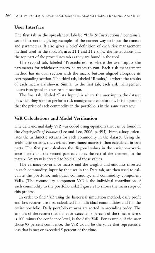
User Interface
The first tab in the spreadsheet, labeled “Info & Instructions,” contains aset of instructions giving examples of the correct way to input the datasetand parameters. It also gives a brief definition of each risk managementmethod used in the tool. Figures 21.1 and 21.2 show the instructions andthe top part of the procedures tab as they are found in the tool.
The second tab, labeled “Procedures,” is where the user inputs theparameters for whichever macro he wants to run. Each risk managementmethod has its own section with the macro buttons aligned alongside itscorresponding section. The third tab, labeled “Results,” is where the resultsof each macro are shown. Similar to the first tab, each risk managementmacro is assigned its own results section.
The final tab, labeled “Data Input,” is where the user inputs the dataseton which they want to perform risk management calculations. It is importantthat the price of each commodity in the portfolio is in the same currency.
VaR Calculations and Model Verification
The delta-normal daily VaR was coded using equations that can be found inthe Encyclopedia of Finance (Lee and Lee, 2006, p. 495). First, a loop calcu-lates the arithmetic returns for each commodity in the dataset. Using thearithmetic returns, the variance-covariance matrix is then calculated in twoparts. The first part calculates the diagonal values in the variance-covari-ance matrix and the second part calculates the rest of the elements in thematrix. An array is created to hold all of these values.
The variance-covariance matrix and the weights and amounts investedin each commodity, input by the user in the Data tab, are then used to cal-culate the portfolio, individual commodity, and commodity componentVaRs. (The commodity component VaR is the individual contribution ofeach commodity to the portfolio risk.) Figure 21.3 shows the main steps ofthis process.
In order to find VaR using the historical simulation method, daily profitand loss returns are first calculated for individual commodities and for theentire portfolio. Daily portfolio returns are sorted in ascending order. Theamount of the return that is met or exceeded x percent of the time, where xis 100 minus the confidence level, is the daily VaR. For example, if the userchose 95 percent confidence, the VaR would be the value that represents aloss that is met or exceeded 5 percent of the time.
306 Part iV FOREIGN EXCHANGE MARKETS, ALGORITHMIC TR ADING, AND RISK

ch
ap
te
r 2
1A
RIS
K-M
ON
ITO
RIN
G T
OO
L D
EDIC
AT
ED t
o C
om
mo
dit
y T
ra
din
g307
Nb. Profit and Loss and ATR data have to be deleted from Sheet1 before other codes can be used
Nb. Steps 2 and 3 are for VaR calculations, Bootstrapping and Stress Testing
Instructions
Instructions for Data Management
Example:
Example:
Example:
Example:
1. Enter the appropriate data in the spaces provided
Instructions for everything other than Data Management and ATR
Instructions for ATR
1. Enter the data in Sheet1 starting with the dates in ‘Column C’ with the commodity prices in the following columns (no gaps in columns). Ensure you enter commodity names in Row 1
2. Press the ‘Start’ button
6. Delete Profit and Loss data in Sheet1 before other codes are used5. Press the button associated with the procedure you want to use4. Go to the ‘Procedures’ section of this worksheet and find the section associated with the procedure you want to use and enter the data needed/follow instructions
3. Delete ATR data from Sheet12. Press the ‘ATR’ button
1. Enter the data in ‘Sheet1’ starting with the dates in ‘Column C’ and the OHLC prices of your commodity after that. Row1must contain headings only. If no headings enter data in Row2
3. After presing the ‘Start’ button the commodity names entered into Sheet1 will appear in the ‘Weights’ and ‘Amount Invested’ sections on this sheet in the order entered.
Ensure the data is of the format most recent date list
Please enter the weights and amount invested for each commodity under the commodity names. Make sure to enter total amount invested
2. For the period please enter the following: d for daily, m for monthly, y for yearly, and v for dividends3. Press the ‘Data Management’ button
................................................................................................................................................................................................................................................................................................................................................................................
................................................................................................................................................................................................................................................................................................................................................................................
Start day:Start month:Start year:
23
2007
C D E FDate
2/26/8712
Gold552
Silver6
Platinum662
C D E FDate
2/26/8712
Opening33
High34
Low31
G orClosing
32
C D E F
2/26/8712 33 34 31
G
32
Gold Silver Platinum Palladium0.25
10000WeightsAmount Invested
0.2510000
0.2510000
0.2510000
Total1
40000
End day:End month:End year:
135
2008
Ticker:Period:
rpha.bed
Figure 21.1 Instructions for Using the Tool

308 Part iV FOREIGN EXCHANGE MARKETS, ALGORITHMIC TR ADING, AND RISK
Nb. Please enter the data needed for your specific procedure before proceding to press the following buttons
Nb. Start month is a month behind; i.e., if you want 6, then enter 5
Nb. Only 95%, 97.5%, and 99% confidence levels can be used for Delta-Normal
ProceduresMacros
Data Management
For everything other than Data Management and ATR
Value at Risk (VaR) Calulations
Profit and Loss (P/L)
Start day:Start month:Start year:
316
2009
Corn Soybeans Soybean Meal Total
0.5500000
WeightsAmount Invested
Has to be entered in decimal form; i.e., 0.95 = 95% VaR
If you want daily VaR then enter1
Confidence level:
Holding Period:
Results for this procedure shall be shown in Sheet1
Needs amounts invested
DataManagement
Initialize Data
Delta-Normal
HistoricalSimulation
Portfolio
Commodity
0.95
1 day(s)
0.25250000
0.25250000
11000000
End day:End month:End year:
317
2009
Ticker:Period:
rpha.bed
Figure 21.2 Procedures
Calculate arithmeticreturns for each
commodity in portfolioand hold in array ofdimension (m-1*c)Square the
arithmetic returnsand hold in array ofdimension (m-1*c)
Multiply arithmetic returns foreach commodity by arithmetic
returns for each othercommodity and hold in array
of dimension (m-1*(c-1)!)
Sum up eachcolumn of the
previous array andhold in array ofdimension (1*c)
Calculate the diagonalvalues of the var/oovarmatrix by multiplyingeach element in the
previous array by (1/m)
Calculate the var/oovarmatrix (minus diagonalvalues) by multiplyingeach element in the
previous array by (1/m)
Create array of dimension (c*c) tohold all elements of var/covar matrix
Calculate portfolioVaR and hold in arrayof dimension (1*1)
*Note: c = number of commodities; m = number of days in estimation period
Calculate individualcommodity VaRand hold in array
of dimension (c*1)
Calculate commoditycomponent VaRand hold in array
of dimension (c*1)
Sum up eachcolumn of the
previous array andhold in array of
dimension (1*(c-1)!)
Delta-Normal VaR
Figure 21.3 VaR Calculation Using the Delta-Normal Method
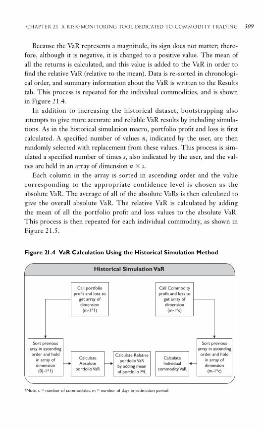
Because the VaR represents a magnitude, its sign does not matter; there-fore, although it is negative, it is changed to a positive value. The mean ofall the returns is calculated, and this value is added to the VaR in order tofind the relative VaR (relative to the mean). Data is re-sorted in chronologi-cal order, and summary information about the VaR is written to the Resultstab. This process is repeated for the individual commodities, and is shownin Figure 21.4.
In addition to increasing the historical dataset, bootstrapping alsoattempts to give more accurate and reliable VaR results by including simula-tions. As in the historical simulation macro, portfolio profit and loss is firstcalculated. A specified number of values n, indicated by the user, are thenrandomly selected with replacement from these values. This process is sim-ulated a specified number of times s, also indicated by the user, and the val-ues are held in an array of dimension n s.
Each column in the array is sorted in ascending order and the valuecorresponding to the appropriate conf idence level is chosen as theabsolute VaR. The average of all of the absolute VaRs is then calculated togive the overall absolute VaR. The relative VaR is calculated by addingthe mean of all the portfolio profit and loss values to the absolute VaR.This process is then repeated for each individual commodity, as shown inFigure 21.5.
chapter 21 A RISK-MONITORING TOOL DEDICATED to Commodity Trading 309
Sort previousaray in ascendingorder and hold
in array ofdimension(0)-1*1)
CalculateAbsolute
portfolio VaR
*Note: c = number of commodities; m = number of days in estimation period
Calculate Relativeportfolio VaR
by adding meanof portfolio P/L
CalculateIndividual
commodity VaR
Sort previousarray in ascendingorder and hold
in array ofdimension(m-1*c)
Call portfolioprofit and loss to
get array ofdimension(m-1*1)
Call Commodityprofit and loss to
get array ofdimension(m-1*c)
Historical Simulation VaR
Figure 21.4 VaR Calculation Using the Historical Simulation Method

In order to verify the effectiveness of these models—delta-normal, his-torical simulation, and bootstrapping historical simulation—backtesting isconducted. VaR is calculated for a user-specified period of time and thisvalue is compared with the next day’s profit and loss return. This isrepeated for another user-specified period of time. For example, if the userwould like to use one trading year’s worth of data (252 days) to calculateVaR and backtest over another 252 days, 252 data points would be used tocalculate the VaR for each of the last 252 days of data in the column.
The positive and negative VaR are recorded as well as the portfolio’sarithmetic return for the next day. If this return does not fall between thepositive and negative VaR, it is considered an exception. The number andmagnitude of exceptions are totaled up, and shown graphically by present-ing those three values—the positive VaR, the negative VaR, and the nextday’s return—on a chart. This allows the user to see when there are excep-tions, whether they are above the positive VaR or below the negative VaR,and their magnitude.
310 Part iV FOREIGN EXCHANGE MARKETS, ALGORITHMIC TR ADING, AND RISK
Randomly select withreplacement n elements
from previous arrayand hold in array of
dimension (n*1)
Call portfolio profitand loss to get
array of dimension(m-1*1)
Portfolio VaR Commodity VaR
Simulate thisprocess s time and
hold in array ofdimension (n*s)
Sort each column inprevious array in
ascending order andhold in array ofdimension (n*s)
Calculate Absoluteportfolio VaR foreach column andhold in array ofdimension (1*s)
Calculatemean Absolute
VaR
CalculateRelative VaR byadding mean ofportfolio P/L
*Note: c = number of commodities; m = number of days in estimation period; n = number of bootstrapped samples wanted; s = number of simulations wanted
Simulate thisprocess s times and
hold in array ofdimension (n*(c*s)
Call Commodityprofit and loss to getarray of dimension
(m-1*c)
Randomly select withreplacement n elements
from each column inprevious array and hold in
array of dimension (n*(c*s))
Calculate VaR ofeach column andhold in array of
dimension (1*(c*s))
Sort each column in previous array in
ascending order andhold in array of
dimension (n*(c*s))
Calculate meanVaR for eachcommodity
Bootstrapped Historical Simulation
Figure 21.5 VaR Calculation Using the Bootstrapping Method

Average True Range (ATR)
The ATR indicator uses the OHLC prices of a commodity. First, themacro calculates the daily true range (DTR) of the dataset by performingthe following operations: high price minus low price, absolute high priceminus previous closing price, and absolute low price minus previous closingprice. This is shown in Equation (21.1), where t is the time horizon formeasuring DTR.
(21.1)
The 14-day ATR is then calculated using Equation (21.2), where v is thetime horizon for measuring ATR.
(21.2)
Lastly, a graph is drawn plotting the ATR readings over the entire dataset,as shown in Figure 21.6.
Moving Averages
This macro works for a portfolio of three commodities and uses one trad-ing year of data, or 252 days. Twelve- and 26-day simple moving averagesare calculated using the Excel moving averages add-in, which computes thefollowing formula:
(21.3)
The MACD line, which is the difference between the two SMAs, is calcu-lated next, and from that the signal line is calculated. The signal line is a
chapter 21 A RISK-MONITORING TOOL DEDICATED to Commodity Trading 311
DTR H L Abs H C Abs L Ct t t t t t t= − − − ∀− −max( , ( ), ( )),1 1 11 14
1 1 1
< ≤
= −
tDTR H L
ATRDTR
ATRATR DTR
tt
vv m
11
14
1
141314
=
=× +
=
−
∑
(( ) ), ∀∀ >v 1
SMAN
pricet t ii
N
=⎛
⎝⎜
⎞
⎠⎟ −
=
∑1
1

nine-day EMA of the MACD line, calculated according to the followingformula:
EMAt ((pricet EMAt1) multiplier) EMAt1 (21.4)
A chart is then drawn, showing the MACD and signal lines and enabling theuser to see the results graphically, as shown in Figure 21.7.
312 Part iV FOREIGN EXCHANGE MARKETS, ALGORITHMIC TR ADING, AND RISK
Calculate ‘High - Low’and hold in array ofdimension (m-1*1)
Calculate first element of‘Daily True Range’ from
previous three arrays usingformula given above
Create array ofdimension (m*1) tohold all elements ofprevious two arrays
Calculate first elementof 14-Day ATR as the
‘average of first 14elements of previous array’
*Note: m = number of data points in estimation period
Hold all values for14-Day ATR in array
of dimension(m-14*1)
Call ‘Graph’ to makea graph of the14-day ATR
Calculate remainingelements of 14-Day ATRusing formula given above
Calculate remaining elementsof ‘Daily True Range’ from theprevious three arrays using
formula given above
Calculate ‘AbsoluteHigh-Previous Close’and hold in array ofdimension (m-1*1)
Calculate ‘AbsoluteLow – Previous Close’
and hold in array ofdimension (m-1*1)
ATR
Figure 21.6 Calculation of Average True Range

The full code for the risk-monitoring tool can be obtained for free by e-mailing the authors.
CONCLUSION
The risk-monitoring tool developed for this project has the following capabili-ties: initializing commodity price data input by the user, calculating VaR usingthe delta-normal method, calculating VaR using historical simulation, boot-strapping historical simulation, model verification by backtesting, calculatingATR, and generating moving averages. In this way, traders who were previ-ously only familiar with technical market indicators can be introduced to VaR.
The risk metric VaR, calculated at 95 percent confidence, quantifies tothe user the amount he can expect to lose 1 day in 20. It can provide a use-ful insight into potential losses for an individual commodity and for theportfolio as a whole; however, it does not take into consideration the poten-tial of extreme outliers. Therefore, VaR can provide a false sense of secu-rity to traders, and according to some it was a factor in losses madethroughout the subprime crisis.
ATR, on the other hand, portrays price volatility that VaR cannot: itlooks at the commodity’s performance over a certain period and determineswhether the commodity is undergoing an active or a quiet trading period.However, it cannot determine the direction or duration of price movementfor a commodity. While it is an effective risk management indicator on itsown, it is much more useful if combined with other risk analysis methods,such as stop and resistance levels. Unfortunately, it is often difficult to findspecific opening, high, low, and closing prices.
chapter 21 A RISK-MONITORING TOOL DEDICATED to Commodity Trading 313
Read in userinputs, set
reference cells
Use one year’s worthof data; delete the rest
Calculate 12- and26-day moving
averages
Calculate MACDand signal lines
Draw a graph for eachcommodity showing
MACD, signal line, andbuy and sell points
Generate a columnincluding “sell” signals
Generate a columnindicating “buy”
signals
MACD
Figure 21.7 Calculation of Moving Averages

The use of multiple moving averages on the same chart in order to gen-erate “buy” and “sell” signals is a tried and tested trading technique. Themoving average with a shorter time period is more sensitive to changingconditions, while the one with longer time period minimizes the effects ofany price irregularities. Using a crossover between the two is more reliablethan acting when one day’s price crosses the moving average, because anygiven price could be an outlier. At the same time, this crossover lags moreand the investor may realize a lower return as a result of waiting for it.
Using VBA in Excel is an effective way to develop a risk-monitoring tooladapted to the commodity market. It is relatively simple to learn and alsoaffordable, as anyone who has access to Microsoft applications does notneed to make any further investment to use software programmed in VBA.Its affordability is important for small companies or individual traders, whomight want the capabilities of big name risk management software butunfortunately do not have the means with which to purchase it. On theother hand, a downside to using VBA is that its computational power issomewhat limited, and as such, it can be slow. Because of this, portfolio sizeand complexity is restricted.
RESOURCES
Albright, S.C. (2007) VBA for Modelers: Developing Decision Support Systemswith Microsoft® Excel. London: Thomson Brooks/Cole.
Borodovsky, L. and Lore, M. (2000) The Professional’s Handbook of FinancialRisk Management. Oxford, UK: Butterworth-Heinemann.
Chernick, M.R. (2008) Bootstrap Methods: A Guide for Practitioners andResearchers, 2nd ed. Hoboken, NJ: John Wiley & Sons.
Lee, A. and Lee, C. (2006) Encyclopedia of Finance. New York: Springer.Jackson, M. and Staunton, M. (2001) Advanced Modelling in Finance Using
Excel and VBA. Chichester, UK: John Wiley & SonsJorion, P. (1997) Value at Risk: The New Benchmark for Controlling Market
Risk. London: McGraw-Hill.Khindanova, I.N. and Rachev, S.T. (2000) Value at Risk: Recent Ad-
vances. Available at: http://www.gloriamundi.org/detailpopup.asp?ID453055174
Linsmeier, T.J. and Pearson, N.D. (1996) Risk Measurement: An Intro-duction to Value at Risk. Working paper, University of Illinois atUrbana-Champaign.
314 Part iV FOREIGN EXCHANGE MARKETS, ALGORITHMIC TR ADING, AND RISK

Wilder, J.W. (1978) New Concepts in Technical Trading Systems. Greensboro,NC: Hunter.
Websites
Wikipedia, Chicago Board of Trade. http://en.wik ipedia.org/wik i/Chicago_board_of_trade (accessed January 2010).
Wikipedia, CME Group. http://en.wikipedia.org/wiki/CME_Group(accessed January 2010).
Wikipedia, MACD. http://en.wikipedia.org/wiki/MACD (accessed January2010).
GloriaMundi, All About Value at Risk™. http://gloriamundi.org (accessedJanuary 2010).
StockCharts. http://stockcharts.com (accessed January 2010).CME Group. http://www.cmegroup.com/trading/commodities/grain-and-
oilseed/corn_quotes_volume_voi.html (accessed January 2010).VBA for Excel (Macros). http://www.excel-vba.com (accessed January
2010).
chapter 21 A RISK-MONITORING TOOL DEDICATED to Commodity Trading 315

This page intentionally left blank

P A R T V
TR ADING VOLUMEAND BEHAVIOR

This page intentionally left blank

319
22C H A P T E R
SecuritiesTrading, AsymmetricInformation, and MarketTransparency
Mark D. Flood, Kees G. Koedijk, Mathijs A. vanDijk, and Irma W. van Leeuwen
ABSTRACT
We examine the consequences of transparency in an experimental multiple-dealer market with asymmetrically informed dealers. Five professional secu-rities traders make a market for a single security. In each trading round, oneof the dealers (the “insider”) is told the security’s true value. We vary bothpre-trade and post-trade transparency by changing the way quote and tradeinformation is published. The insider’s profits are greatest when price effi-ciency is lowest. Price efficiency, in turn, is reduced by pre-trade trans-parency and increased by post-trade transparency. Market liquidity,measured by dealers’ bid-ask spreads, is improved by pre-trade trans-parency and reduced by post-trade transparency.

INTRODUCTION
Information is central to the structure and performance of financial markets.Indeed, a primary function of financial markets is to assemble and digestinformation into an accurate valuation of investment prospects. The interac-tions among participants—the brokers, dealers, market makers, and special-ists transacting on exchange floors and over-the-counter networks—arecentral in this regard. Asymmetric information is thus of obvious impor-tance; the ability of financial markets to weigh information from disparatesources and impound it in prices is basic to their function. We consider therole of asymmetric information across dealers in an experimental multiple-dealer securities market, and specifically its impact on market performanceand the impact of the institutional structure on information aggregation anddissemination.
Asymmetric information has well-documented and substantial effects onthe performance of financial markets, with “insider trading” as the mostimportant example. We distinguish sharply, however, between traditionalcorporate insiders and securities dealers who are better informed than theirpeers in a multiple-dealer environment. The nature of interdealer informa-tional asymmetries is fundamentally different from those generated by cor-porate insiders. Interdealer asymmetries typically arise from information,such as private order f low or the rumor mill, that should already beimpounded in prices in a semi-strong-form efficient market. On the otherhand, the information available to corporate insiders should only beimpounded in prices if markets are fully strong-form efficient.1 An impor-tant empirical question concerns the benefits of interdealer trade. If marketsare not already semi-strong-form efficient, interdealer trading can impoundinformation from dealers’ private order flow, improving price quality.
We are interested in the interaction between interdealer informationasymmetries and microstructural rules for publication of quote details andtransaction details, because this interaction affects the revelation and aggre-gation of information. For example, in the 1990s, market makers on theStock Exchange Automated Quotation system in London argued fordelayed publication of the details of trades, ostensibly to encourage the pro-vision of liquidity to investors for large transactions (see Office of FairTrading, 1994). Such delays create interdealer information asymmetries,allowing an affected dealer to unwind her resulting inventory before hercompetitors recognize her predicament. The informational question thus
320 PART V TR ADING VOLUME A ND BEHAVIOR

extends to issues of dealer inventories, risk bearing, and capitalization. Morerecently, some exchanges have facilitated “flash trades,” which allow certainparticipants very brief advanced knowledge of incoming orders; once again,the rationale offered by participants is that the mechanism attracts tradingvolume and improves liquidity (see The Economist, 2009).
We consider here the publication of both transaction details (post-tradetransparency, e.g., via a public ticker) and live quotes (pre-trade transparency,e.g., a public limit-order book), and focus on price discovery and transac-tion costs. As Glosten (1999) emphasizes, the issues and results in this areacan be complex and counterintuitive.2 The obvious presumption is thatincreased transparency would always simultaneously speed price discoveryand facilitate counterparty matching and therefore improve both price effi-ciency and transaction costs. The empirical picture is more complex, how-ever, especially regarding pre-trade transparency. Boehmer, Saar, and Yu(2005), for example, find that an increase in pre-trade transparency throughexpanded availability of the NYSE’s OpenBook service is associated bothwith a decline in effective spreads and an improvement in the informationalefficiency of prices. Madhavan, Porter, and Weaver (2005) find that in-creased pre-trade transparency on the Toronto Stock Exchange increasesthe risk to limit orders of being “picked off” by other traders, leading towider spreads, lower liquidity, and lower stock prices. Simaan, Weaver, andWhitcomb (2003) find a similar relation between pre-trade transparencyand posted spreads in the NASDAQ market. Hendershott and Jones (2005)find that a decrease in pre-trade transparency on the Island electronic com-munications network is associated with increased autocorrelations in prices,suggesting that price discovery deteriorates when transparency falls. Theempirical situation for post-trade transparency is more clear-cut. Edwards,Harris, and Piwowar (2007), Bessembinder, Maxwell, and Venkataraman(2006), and Goldstein, Hotchkiss, and Sirri (2007), all find that increasedpost-trade transparency in the U.S. corporate bond market is associatedwith narrower spreads and/or lower estimated transaction costs.
It is difficult to study the interaction of microstructure and asymmetricinformation using empirical data. Even if it were possible to identify asym-metries, it would still not be feasible to isolate the effect of a static tradingmechanism. We therefore adopt an experimental methodology (see Sunder,1995 for a survey). Results from prior experimental studies mirror some ofthe complexity of the empirical work. Bloomfield and O’Hara (1999) and
chapter 22 TR ADING, ASYMMETRIC INFORMATION, and Transparency 321

Flood, Huisman, Koedijk, and Röell (FHKR, 1997) both find that post-trade transparency does speed price discovery. On the other hand, Flood,Huisman, Koedijk, and Mahieu (FHKM, 1999) f ind that increased pre-trade transparency actually slows price discovery in a multiple-dealermarket; they conclude that dealers in an opaque market reprice moreaggressively to attract order flow. In contrast, dealers in a pre-trade trans-parent market can typically offer much smaller price improvements andnonetheless guarantee a place atop the public limit order book. Our studydiffers from most experimental double-auction studies (but not all; seeForsythe, Palfrey, and Plott, 1982; and Plott and Sunder, 1982), in that ourtraders can both buy and sell the asset. Moreover, all our dealers act as mar-ket makers, providing bid-ask quotes to other dealers at all times.
Our market framework is based on Glosten and Milgrom’s (1985) model;it is a quote-driven, continuous securities market in which five market mak-ers trade a single imaginary security. We use three groups of professionalsecurities dealers as experimental subjects. The market makers set quotesand trade with each other and with computerized external customers. Thelatter are either informed traders or noise traders. In each trading round,one of the market makers is randomly chosen to be the “insider,” whoknows the underlying value of the security. Since he is a market maker, heboth trades and competes on price with the other market makers. In theseexperiments, we use the notion of pre-trade and post-trade transparency todistinguish between four different trading mechanisms. Following Paganoand Röell (1996), we define pre-trade transparency as the amount of quotedprice information available to market makers, and post-trade transparencyas the amount of transaction information available to market makers. We measure the relative private gains (in terms of insider profits) and publicgains (in terms of speed of price discovery and size of dealer spreads) associ-ated with various trading mechanisms when information asymmetries are present.
The contribution of this study is three-fold. First, we consider four different trading mechanisms in which we explicitly distinguish betweenpre-trade and post-trade transparency in our analysis. (Other studies exam-ining insider trading in different trading mechanisms use a quite generalnotion of transparency; see, e.g., Pagano and Röell, 1996, and Schnitzlein,1996.) The distinction between price and transaction information is impor-tant, as the different types of information flows have different effects onmarket outcomes. It is also important in terms of intermarket competition,
322 PART V TR ADING VOLUME A ND BEHAVIOR
as competing exchanges worldwide implement trading mechanisms thatindeed differ in the levels of both pre-trade and post-trade transparency.
Second, we use an experimental setting in which continuous trading ispossible. This provides us with extensive time-series data: thousands oftransactions and hundreds of quote settings for each of the trading mecha-nisms. Most experimental studies on microstructure have only a fraction ofthis available. Moreover, we use professional market makers as the subjectsin our experiment. This is an important advantage over experiments usingstudents as subjects.
Third, we offer an alternative view of asymmetric information by givingthe insider a different role compared with other studies (e.g., Kyle, 1985;Glosten and Milgrom, 1985; Easley and O’Hara, 1992; and Schnitzlein,1996). Generally, the insider is regarded as an external customer submittingorders to the financial market. Market makers then compete for the ordervia their quoted prices, and the order is typically executed against the bestprice. In contrast, our insider is a market maker, competing directly onprice with other market makers. (Lyons, 1996, for example, examines therole of private order flow as a source of interdealer information asymme-tries in a multiple-dealer market.) Our setup is closest institutionally tomultiple-dealer markets such as NASDAQ, the London Stock Exchange, orthe foreign exchange market.
We find an inverse connection between insider profits and price efficiency.Slow price discovery allows insiders greater opportunities to accumulatespeculative inventories at advantageous prices. At the same time, however,we find that post-trade transparency (e.g., a public ticker) improves pricediscovery, while pre-trade transparency reduces price discovery. Conse-quently, post-trade transparency reduces insider profits, while pre-tradetransparency increases them. Meanwhile, increased pre-trade transparencyreduces dealers’ uncertainty and reduces market liquidity (as measured bybid-ask spreads), while post-trade transparency induces dealers to competefor private order flow, thus reducing spreads and increasing liquidity.
EXPERIMENTAL DESIGN AND TERMINOLOGY
This section briefly presents the experimental setup. For a full descriptionof the experiments we refer to Flood, Koedijk, van Dijk, and van Leeuwen(FKDL, 2002), which is an earlier working paper version of this study thatcontains all the details about the experimental setup. Our tests involve a
chapter 22 TR ADING, ASYMMETRIC INFORMATION, and Transparency 323

computerized experimental securities market in which a number of humandealers (including one with an information advantage, the “insider”) tradecontinuously with each other and a computerized, non-market-making cus-tomer (the “robot”) for a single imaginary security.
Market Design
Our experimental microstructure is a continuous multiple-dealer version ofthe pure dealership market used by Glosten and Milgrom (1985). This market is quote driven, in the sense that the specialist first sets quotes andthen confronts orders from traders. This is the main difference betweenour experimental design and Kyle’s (1985) order-driven framework inwhich the market maker determines a market-clearing price for a batch oforders. (See Madhavan, 1992 for an overview of the differences betweenquote-driven and order-driven markets.)
The Role of the Dealers
A priori, the security’s true (underlying) value is unknown to all humandealers but one. Each participant is the insider in either two or threerounds. All dealers are informed that there is exactly one insider in everyround. The true value is revealed publicly at the end of each trading round.Dealers are instructed to maximize their end-of-round wealth by trading onthe security. Wealth is expressed in esquires (a fictional numéraire cur-rency). Dealers can gain or lose wealth during each round by buying andselling the security (i.e., by jobbing) and by building a long or short inven-tory of the security that is converted into cash at the security’s true value atthe end of each round (speculating). The true value is set at random anddiffers in each practice and session round (the values are available from theauthors). Trading in every round can be regarded as trading for a new secu-rity. At the start of each round, the non-insider only knows that the truevalue in that round is uniformly distributed over [1,200].
Quoting, Trading, and Pre-Trade Transparency
At the start of each round, each dealer is obliged to enter a quote (that is, abid price and an ask price) within 10 seconds. Dealers who fail to enter aninitial quote within the first 10 seconds are penalized at the rate of 10esquires per second after that, until an initial quote is entered. Thereafter,
324 PART V TR ADING VOLUME A ND BEHAVIOR

every dealer always has a quote outstanding, at which the other marketmakers and the robot can trade. The maximum individual spread is limitedto 30 esquires.
The primary parameters in our experiments are the level of pre-tradetransparency and the level of post-trade transparency. Both variables canassume one of two values: high or low. When the level of pre-trade trans-parency is high (“full quote disclosure”), all outstanding price quotes appearcontinuously on the trading screen of each market maker. Bid and askprices appear in separate queues in the center of the screen. Next to everyprice, the identity of the dealer (human or robot) who quoted this priceappears. If at any time the bid (ask) price of several dealers is the same, thenthe most recently quoted price is at the top. When a dealer opts to buy(sell), he automatically does so at the lowest (highest) quoted ask (bid) price.
When the level of pre-trade transparency is low (“no quote disclosure”),no price information is publicly available. Instead, prices and transactionsare communicated on a strictly bilateral basis. Dealers call each other toobtain price quotes. The dealer who receives a call does not respondactively. She does not even notice that she is being called; instead, her mostrecently quoted bid and ask prices automatically appear on the caller’sscreen. Then, the caller has the option to buy, sell, or do nothing.
Transaction Information and Post-Trade Transparency
A high level of post-trade transparency implies that there is full and imme-diate trade disclosure. The information appears in a transaction historywindow on the trading screen and consists of the identities of the buyer andseller, the transaction size (which always equals one share in our setup) andthe price at which the transaction cleared. When the level of post-tradetransparency is low, only transactions in which a particular dealer wasinvolved are listed in his window. There is no delay in trade disclosure.
Robot Behavior
The robot is programmed to trade every 7 seconds against the best pricesin the market. Prior to each robot transaction, it is determined by chancewhether the trade is an informed or an uninformed one. The noise level—i.e., the a priori probability α that a trade is informed—equals 0.5 in allrounds. At the start of the experiment, the dealers are told this probability.
chapter 22 TR ADING, ASYMMETRIC INFORMATION, and Transparency 325

Given their knowledge of the probability that a robot is informed (α), dealers may be able to filter relevant price information by observing robottransactions.
If the robot initiates an informed trade, it buys (sells) if the lowest askprice (highest bid price) at that time is below (above) the true value of thesecurity. The robot does not trade if quoted bid-ask spreads surround the true value. Note that the robot maximizes its expected profits only atthe trade level; there is no dynamic strategy. If a robot initiates an unin-formed trade, a binomial random draw (with probability one half ) deter-mines whether the robot sells or buys; if it sells (buys), it does so against thehighest bid price (lowest ask price) available.
Rounds and Parameters
We ran the experiments with three groups of human subjects. Each grouptraded in two “sessions” consisting of six 5-minute trading rounds per ses-sion. To control for possible learning effects, the first group started with asession with no quote disclosure, and then moved on to a session of fullquote disclosure; the second group followed the opposite sequence. Thethird group followed the same sequence as the first. Within each session,post-trade transparency alternated between low and high from round toround. Each trading session followed two 5-minute practice rounds, one inwhich the level of post-trade transparency was low and the other in which itwas high. The practice rounds acquaint the subjects with the trading systemand provide a chance to ask questions. In the “real” (i.e., the non-practice)rounds, subjects were paid for their results. The data reported here comefrom the real sessions. At the end of each round, all dealers learn their finalwealth. Esquires are translated into Dutch guilders according to a paymentscheme that is explained to the dealers before the start of the experiment (1 USD 1.75 NLG). In every round, 15 guilders are divided among allmarket makers, making this a fixed-sum game. Details on the paymentscheme are provided in FKDL (2002).
DATA
The data were collected from experiments held at the laboratory of theCenter for Research in Experimental Economics and Political DecisionMaking (CREED) at the University of Amsterdam. The subjects in the
326 PART V TR ADING VOLUME A ND BEHAVIOR

first experiment, conducted on January 27, 1997, are five professionaloption traders from Optiver. In the second experiment, conducted on 3 February 1997, five professional equity traders from ABN Amro Bank, deGenerale Bank, and Oudhoff Effecten participated. These subjects acted asmarket makers in 12 independent rounds, divided into two six-round ses-sions. The third replication, involving five professional options traders fromAmsterdam Options Traders, was conducted on April 21, 1999. Unfortu-nately, an operating system failure at the CREED lab forced us to abandonthis set of replications before we were done. Eight rounds of usable datawere produced, however. Table 22.1 presents some basic summary statistics.
chapter 22 TR ADING, ASYMMETRIC INFORMATION, and Transparency 327
Table 22.1 Summary Statistics for Each Trading Mechanism
Variable LL LH HL HH
Number of Quotes Set 47.3 43.8 67.2 62.4
Number of TradesTotal 248.1 445.8 528.9 516.0
Outsiders 108.8 150.5 191.1 202.4
Insider 104.0 256.6 302.6 279.0
Robot 35.4 38.6 35.1 34.6
Average Dealer Spreads
Outsiders 23.9 25.1 20.1 21.1
Insider 21.8 26.4 22.8 17.3
Average End-of-Round Capital
Outsiders 518.1 1737.5 2024.5 358.6
Insider 1837.3 6361.6 7722.5 1337.9
Price Discovery
Time to Convergence* 185.8 241.3 138.6 105.5
Percentage price error†
after 100 seconds 0.39 0.57 0.39 0.32
after 200 seconds 0.12 0.23 0.32 0.15
after 300 seconds 0.06 0.09 0.18 0.14
In Table 22.1, the summary statistics for individual rounds are averaged over all three groups and eightrounds to obtain summary statistics for the four trading mechanisms.
LLlow pre-trade and low post-trade; LHlow pre-trade and high post-trade; HLhigh pre-trade and lowpost-trade; HHhigh pre-trade and high post-trade.
*Average number of seconds until the average quote midpoint for all dealers has converged to less than 5esquires away from the underlying true value.
†Average price error after t seconds, divided by the average price error after 20 seconds.
More detailed tables with the settings in each round and summary statisticsfor individual rounds and the three groups of subjects are available inFKDL (2002).
RESULTS
In this section, we analyze the speed of price discovery, the level of insiderprofitability, and the bid-ask spreads (as measures of efficiency, unfairness,and liquidity, respectively) as a function of pre-trade and post-trade trans-parency. We consider the full-factorial 2 2 matrix of transparencyarrangements. We adopt a two-letter notational shorthand, in which thefirst letter indicates pre-trade transparency and the second letter indicatespost-trade transparency. For example, “HL” indicates a high pre-trade andlow post-trade transparency regime.
Price Efficiency
Following Bloomfield and O’Hara (1999), FHKR (1997), and FHKM(1999), we use price errors to measure the informational efficiency of pricesin the market. We define price errors as the absolute difference between theaverage midpoint of all outstanding quotes and the underlying value of thesecurity. Our hypothesis on the effect of transparency on price efficiency isbased on the results of, among others, Bloomfield and O’Hara (1999),FHKR (1997), and Pagano and Röell (1996). These studies find thatincreasing post-trade transparency leads to greater efficiency. The pre-sumption would be that it is relatively hard for insiders to hide privateinformation when transaction information is widely available to the non-insider market makers. In contrast, FHKM (1999) find a search-costeffect that causes increased pre-trade transparency to reduce efficiency in amultiple-dealer market.
Figure 22.1 shows the average price error time path for each of the fourtrading mechanisms. Since the only ex ante information that the unin-formed market makers have about the underlying value is that it liesbetween 1 and 200, their best initial guess should be that the underlyingvalue is around 100. This guess is reflected in the value of the price error atthe beginning of each round, which is generally close to the absolute differ-ence between the true value and 100. As shown in Figure 22.1 and the lastpanel of Table 22.1, price errors clearly move towards zero after the first 20 seconds, a pattern observed in all four trading mechanisms.
328 PART V TR ADING VOLUME A ND BEHAVIOR

Price errors decline as more information about the underlying value ofthe security is brought into the market. By definition, the better the mar-ket’s ability to transmit information, the faster price errors decline. Whilethe average price error paths in Figure 22.1 disguise considerable round-to-round variation in initial errors and convergence rates, the most andleast transparent cases (HH and LL) appear to perform well relative to theothers. This supposition is borne out by a more controlled statistical analy-sis. In Table 22.2, we average price errors across all three groups and allrounds with a common transparency regime. Averages of dealer spreadmidpoints are taken at 50-second intervals throughout the trading round(plus an early reading after the first 20 seconds of trading), and are nor-malized by the starting error for the round. (The starting error is definedas abs(100 – TrueValue), since the expected starting quote for the unin-formed dealers is 100.) Normalization compensates for differences in the
chapter 22 TR ADING, ASYMMETRIC INFORMATION, and Transparency 329
70
low, high
high, low
60
50
40
30
20
10
01 26 51 76 101 126 151
Time (in seconds)
Pri
ce E
rro
r
176 201 226 251 276
high, high
low, low
Figure 22.1 Price Errors
Figure 22.1 shows the average price errors for each combination of transparency variables; e.g., “low, high”refers to low pre-trade and high post-trade transparency. Price errors are defined as the absolute differencebetween the true value of the security and the average midpoint of outstanding quotes. The price errors areaveraged across all rounds with the specified combination of transparency variables. The first 20 seconds ofeach round are omitted, to allow time for all dealers to submit their first quotes.

true value of the security across rounds, allowing meaningful averages andcomparisons. The bulk of price discovery occurs during the first 150 sec-onds of trading, and the HH and LL regimes clearly outperform HL andLH over this interval. After 150 seconds, average price errors are overtwice as large for HL (38 percent) and LH (36 percent) as they are foreither HH (17 percent) or LL (15 percent).
More formally, we estimate an individual effects panel model to examinethe price efficiency in each of the four different trading mechanisms used inthe experiments. We regress the price errors obtained in all 32 rounds on aconstant, 32 individual-round dummies and four trend dummies. Thedummy variables are included to isolate the effects of transparency. Theestimated equation is
(22.1)
where t denotes time in seconds and r the trading round, Ptr is the averagemidpoint over all bid and ask quotes at time t, I(·) is a dummy variable fortrading round and trading mechanism, and εtr is an independent and identi-cally distributed (i.i.d.) error term. Since dealers’ behavior changes after pricediscovery is achieved—trends in prices typically level off abruptly at thispoint—we discard observations after the point in time at which price errors
330 PART V TR ADING VOLUME A ND BEHAVIOR
Table 22.2 Normalized Price Errors in Different Trading Mechanisms
Time (in sec) LL LH HL HH
50 0.58 0.78 0.65 0.48
100 0.33 0.56 0.44 0.25
150 0.15 0.36 0.38 0.17
200 0.11 0.22 0.35 0.13
250 0.08 0.13 0.27 0.14
300 0.05 0.08 0.22 0.11
Table 22.2 presents normalized price errors for four different transparency regimes. The normalized priceerrors are based on the absolute difference between the true value of the security in each round and theaverage midpoint of all outstanding quotes. The errors are then averaged over eight rounds to obtain theaverage price errors for each trading mechanism. The results are corrected for the average initial price errorin each transparency regime, so that price errors are directly comparable across trading mechanisms. Theinitial price error is defined as abs (100 – TrueValue).
LLlow pre-trade and low post-trade; LHlow pre-trade and high post-trade; HLhigh pre-trade and lowpost-trade; HHhigh pre-trade and high post-trade.
P I Itr r i
ik
k
TrueValue r i r k t− = + = + ==
∑β β β01
32
( ) ( )==
∑ +LL LH HL HH
tr, , ,
ε

have converged to a value less than or equal to 5. Moreover, we omit transac-tions completed in the first 20 seconds of each trading round to ensure thatall market makers have submitted bid and ask quotes. Ordinary least squares(OLS) estimates for Equation (22.1) are presented in Table 22.3. Larger neg-ative values for the slope coefficient imply faster price discovery. The estimates of the 32 individual-round dummies represent differences in theunderlying value in each round and the identity of the insider. They are omit-ted to conserve space.
Table 22.3 generally confirms the conclusions from Table 22.2, with theexception that the LL regime does not perform relatively as well in theregression analysis as it did in Table 22.2. Table 22.3 thus largely supportsthe hypothesis that efficiency is greater when transparency is higher. Theresults show a clear ranking of the different trading mechanisms, althoughestimates of the slope coefficients in Table 22.3 are not significantly differ-ent from one another at a 5 percent level.3
The exception to the notion that more transparency is better is theleast transparent microstructure (LL), in which efficiency is better thanin the case with high pre-trade and low post-trade transparency (HL);this difference is marginally statistically significant. This confirms the
chapter 22 TR ADING, ASYMMETRIC INFORMATION, and Transparency 331
Table 22.3 Price Efficiency
Pre-Trade Post-Trade Estimated EstimatedTransparency Transparency Intercept Slope Coefficient
LL Low Low 0.207*
(0.030)
LH Low High β0: 57.72* 0.228*
(2.449) (0.034)
HL High Low 0.138*
(0.021)
HH High High 0.317*
(0.141)
Table 22.3 presents the estimated intercept and the coefficients of the trading mechanism dummies from thefixed effects panel model depicted in Equation (22.1). Robust standard errors are presented in parentheses.Significance at the 5 percent level is denoted by*. The number of data points is 4,535. The R-squared of theregression is equal to 0.756.
LLlow pre-trade and low post-trade; LHlow pre-trade and high post-trade; HLhigh pre-trade and lowpost-trade; HHhigh pre-trade and high post-trade.
*Significant at 5 percent level.

earlier work of FHKM (1999), who find that price discovery is fasterunder LL than HL; they argue that search costs can explain this counter-intuitive result, as high pre-trade transparency reduces the incentives foraggressive price improvements. The results of Table 22.3 also confirm theconclusions of FHKR (1997), who find that price discovery is faster underLH than LL.
Lastly, we consider the implications of conditioning on only one of thetransparency variables at a time. Row A of Table 22.4 reports the results ofestimating a modified version of Equation (22.1), in which there are onlytwo transparency dummies, based on the degree of pre-trade transparency(i.e., the HL and HH and the LL and LH rounds are pooled). The differ-ence across coefficients for the pooled groups is marginally significant, andthe search-cost effect described by FHKM (1999) appears to dominate:price discovery is faster when pre-trade transparency is low. Similarly, rowB pools the HL and LL rounds (as well as the LH and HH rounds) toexamine the impact of post-trade transparency. In this case, the trans-parency effect described by FHKR (1997) seems to dominate, as price dis-covery is faster when post-trade transparency is high. This difference is alsomarginally statistically significant.
332 PART V TR ADING VOLUME A ND BEHAVIOR
Table 22.4 Pooled Effects of Pre-Trade and Post-Trade Transparency onEfficiency
Estimated Slope Estimate Slope EstimateRegression Intercept Low Transparency High Transparency
A: Pre-trade transparency 57.053* 0.221* 0.160*
(2.162) (0.023) (0.026)
B: Post-trade transparency 57.146* 0.170* 0.235*
(2.400) (0.021) (0.033)
In the fixed-effects panel model depicted in the first row (case A) of Table 22.4, LL and LH rounds arepooled (first column), as are HL and HH (second column), to examine the effect of conditioning solely onpre-trade transparency. In the second row (case B), LL and HL are pooled, as are LH and HH for a similaranalysis of the effect post-trade transparency. Robust standard errors are in parentheses. Significance at the5 percent level is denoted by *. The differences between low-transparency and high-transparency estimatesare not significantly different from zero at the 95 percent confidence level in either case A or B. The numberof data points is 4,535. The R-squared of regression A (B) is equal to 0.748 (0.750).
LLlow pre-trade and low post-trade; LHlow pre-trade and high post-trade; HLhigh pre-trade and lowpost-trade; HHhigh pre-trade and high post-trade.
*Significant at 5 percent level.

Insider Profits
Our evidence thus far indicates that the speed of price discovery is posi-tively dependent on market transparency, with the exception that the leasttransparent regime (LL) performs relatively well in this regard. With thisexception, then, we expect a generally inverse relation between insider prof-its and transparency, since insider profitability should be inversely related tothe speed of price discovery (faster price discovery reduces the insider’sability to acquire inventory at advantageous prices). This expectation isconsistent with the conclusions of Bloomfield and O’Hara (1999) andPagano and Röell (1996).
When the true value is extreme (i.e., far from 100), insiders are likely tomake larger profits than when it is moderate. As this effect is not due totransparency differences, we normalize total insider profits by the absolutedifference between the true value and 100 in each round. Moreover, welook at both average insider profits and average insider profits per transac-tion. Although it does not affect our conclusions, we regard the latter num-ber as more meaningful, as the number of transactions differs substantiallyacross trading mechanisms (search costs impose a logistical obstacle thatreduces transaction rates substantially in the LL case). The penultimatesection of Table 22.1 presents insider profits (and average outsider losses)under each trading mechanism, averaged across all rounds. Unsurprisingly,outsider losses are closely related to insider profits. More importantly,insider profits are smallest in the most transparent market (HH), which wasalso the market in which price discovery occurred most quickly. Interest-ingly, however, the least transparent market (LL) shows similarly smallinsider profits, a fact consistent with its relatively speedy price discovery,established in the preceding subsection.
We again estimate a fixed effects panel model in which we regress totalprofits per transaction in each of 32 rounds on four trading mechanismdummies. The model is given in Equation 22.2.
(22.2)
where r denotes the trading round, πr is the average insider profit (eithernormalized by the number of transactions or non-normalized) in round
chapter 22 TR ADING, ASYMMETRIC INFORMATION, and Transparency 333
πβ βr
ri
ik
k LTrueValuer i r k
100I I
−= = + =
= =
∑1
32
( ) ( )LL LH HL HH
tr, , ,∑ +ε

r, I(·) is a dummy variable for trading mechanism and εr is an i.i.d. errorterm. OLS estimates of Equation (22.2) appear in Table 22.5. Estimates ofthe 32 individual-round dummies are omitted from the table to conservespace. Again, we see that insider profits are lowest in the most transparent(HH) and least transparent (LL) cases.4 On the other hand, insiders are bestoff in the mixed-transparency cases (HL and LH). The pairwise differencesin regression slope coefficients between the HH case and each of the twomixed-transparency cases (i.e., HH vs. HL, and HH vs. LH) are marginallysignificant. We conclude that insider profitability is inversely and causallyrelated to the speed of price discovery in the market.
As with price discovery, we also consider the implications of condition-ing on only one transparency variable at a time. Table 22.6 reports insiderprofits averaged across each subsample of rounds. Row A of Table 22.6pools results based on pre-trade transparency, with the pooled LL and LHresults (pooled HL and HH results) in the first (second) column. Row Bsimilarly pools LL and HL (LH and HH) in the first (second) column.Although the standard errors are too large for either of the intercolumndifferences to be statistically significant, the pattern in the calculated aver-ages fits neatly with the results in Table 22.4. We confirm our conclusionthat price discovery is the determining factor for our insider profitabilityresults.
334 PART V TR ADING VOLUME A ND BEHAVIOR
Table 22.5 Insider Profits
Pre-Trade Post-Trade Profits perTransparency Transparency Raw Profits Transaction
Low Low 31.43* 0.2657*
(20.84) (0.0704)
Low High 91.07* 0.3608*
(20.84) (0.0704)
High Low 115.25* 0.3554*
(20.84) (0.0704)
High High 34.16* 0.1957*
(20.84) (0.0704)
*Significant at 5 percent level.
Table 22.5 depicts the fixed effects panel coefficients for the trading mechanism dummies in Equation (22.2).For the first column, πr is the coefficient on total insider profits; for the second column, πr is the coefficienton total insider profits divided by the total number of insider transactions. The data is pooled over 32 rounds.Robust standard errors appear in parentheses. Significance at the 5 percent level is denoted by*. The numberof observations is equal to 32. The R-squared amounts to 0.301 for the raw profits and 0.119 for the profitsper transaction.

In sum, the results for insider profits show a clear negative relationbetween insider profits and the speed of price discovery, as anticipated.However, because the relation between price discovery and transparency isa nonlinear one, the relation between insider profits and transparency issimilarly nonlinear.
Spreads
The spread between market makers’ bid and ask quotes is generally assumedto consist of three different components: order-processing costs, inventory-holding costs, and adverse-selection costs. The first two components arenominally equal to zero in our experiments, and we focus on the latter. The standard adverse-selection component represents compensation to thedealer for losses to informed investors. However, a number of papers (e.g.,Madhavan, 1995) argue that dealers in a multiple-dealer market should nar-row their spreads in an effort to “purchase” informative order flow, with thegoal of exploiting the resulting information in subsequent trading, a tacticthat should be enforced by interdealer competition. Thus, adverse-selectioncosts subsume both the degree of uncertainty in the market and the degreeof (imperfect) competition.
The existing literature also indicates that an explicit distinction betweenpre-trade and post-trade transparency is necessary when examining the rela-tion between transparency and bid-ask spreads. Pagano and Röell (1996) findthat the spread size decreases when more price information is available in themarket. The argument is that uncertainty decreases when market makers
chapter 22 TR ADING, ASYMMETRIC INFORMATION, and Transparency 335
Table 22.6 Effects of Pre-Trade and Post-Trade Transparency on AverageProfits
Average Low Average HighTransparency Variable Transparency Transparency
A: Pre-trade transparency 4,099 4,530
(3,933) (6,784)
B: Post-trade transparency 4,780 3,850
(6,524) (4,309)
Table 22.6 presents the effect of transparency on insider profits by averaging the insider profits over twodifferent transparency regimes. In the first row (case A), average insider profits in LL and LH rounds arecomputed (first column), as are HL and HH (second column), to examine the effect of conditioning solely onpre-trade transparency. In the second row (case B), average insider profits in LL and HL are calculated, asare LH and HH for a similar analysis of the effect post-trade transparency. Standard deviations are inparentheses.

know more about each other’s quotes. On the other hand, Bloomfield andO’Hara (1999) find that spreads increase when more transaction informationbecomes available in the market. Madhavan’s (1995) model concludes thatmarket makers compete more fiercely when they cannot observe other marketmakers’ transactions, since in this case they must attract transactions tothemselves to gain the information implicit in the order flow. We thus conjec-ture that reduced pricing uncertainty under pre-trade transparency shouldreduce spreads, while reduced competition under post-trade transparencyshould increase them. This conjecture translates to the following fourhypotheses: (1) SLL SHL; (2) SLH SHH; (3) SHH SHL; and (4) SLH SLL;where Sk is the average spread size under trading regime k.
Figure 22.2 shows the average outsider spreads in the four differentmicrostructures for all three groups of subjects. The average spread in eachtrading round is defined as the average size of the spread between the bid
336 PART V TR ADING VOLUME A ND BEHAVIOR
30
25
20
15
10
5
01 26 51 76 101 126
Time (in seconds)
Spr
ead
Siz
e
151 176 201 226 251 276
low, highlow, low
high, lowhigh, high
Figure 22.2 Dealer Spreads
Figure 22.2 shows the average spread size in each of the trading mechanisms, measured as the average bid-ask spread of all outside dealers in the relevant trading rounds. None of our spread results is changedmarkedly by including or excluding the insider. The initial spreads are high and similar in each tradingmechanism, but spreads decrease as information is brought into the market over time. The spreads arenearly uniformly consistent with our hypothesis. For at least the first 230 seconds of trading, the averagespread size is lowest when pre-trade transparency is high and post-trade transparency is low, indicating thatuncertainty is relatively low and competition relatively severe. The reverse holds for the LH market, inwhich spreads are relatively large.

and ask quotes of all market makers. The lines in this graph were con-structed by averaging the spreads of eight individual rounds with the sametrading mechanism. The first 20 seconds of each trading round were omit-ted from the calculation, as dealers used this time period to enter their firstbid and ask quotes.
To buttress the evidence in Figure 22.2, Table 22.7 presents the averageoutsider spreads pooled for all trading rounds with the specified trans-parency treatment. For example, row A of Table 22.7 presents in the first(second) column the average outsider spread for all LL and LH (HL andHH) rounds. As predicted, increased pre-trade transparency narrows dealerspreads. Similarly, in row B, we see that increased post-trade transparencyincreases spreads. The predictions of our hypothesis continue to hold undera finer-grained analysis. Thus, on average, SLL 23.9, SLH 25.1, SHL
20.1, and SHH 21.1. Although neither of the intercolumn differences inTable 22.7 is statistically significant at the 5 percent level, our hypothesis isnonetheless clearly supported by the available evidence.
CONCLUSION
In this study, we follow the recommendations of Leland (1992), Pagano andRöell (1996), and Schnitzlein (1996) to examine the extent to which marketmicrostructure interacts with asymmetric information to affect market per-formance. Specifically, we consider an experimental multiple-dealer marketin which one of the dealers begins with fundamental information unavailableto the other dealers. We create four different trading mechanisms by varyingthe following two transparency rules: the pre-trade publication of dealer
chapter 22 TR ADING, ASYMMETRIC INFORMATION, and Transparency 337
Table 22.7 Effects of Pre and Post-Trade Transparency on Average Spreads
Average Low Average HighTransparency Variable Transparency Transparency
A: Pre-trade transparency 24.5 20.6
(2.39) (3.65)
B: Post-trade transparency 22.0 23.1
(3.88) (3.36)
Table 22.7 presents the effect of transparency on dealer spreads by averaging the spreads over two differenttransparency regimes. In the first row (case A), average outsider spreads in LL and LH rounds are computed(first column), as are HL and HH (second column), to examine the effect of conditioning solely on pre-tradetransparency. In the second row (case B), average outsider spreads in LL and HL are calculated, as are LHand HH for a similar analysis of the effect post-trade transparency. Standard deviations are in parentheses.

quotes (private information or broadcast) and the post-trade publication oftransactions (public ticker or private information). The characteristics of thetrading mechanism affect how difficult it is for uninformed dealers to detectan insider and infer his strategies; conversely, they affect the ability of theinsider to exploit his informational advantage.
We obtain our data from a series of 5-minute trading rounds for threegroups of five professional securities traders. Our results clearly indicate aninverse connection between insider profits and the price efficiency of themarket. Slow price discovery allows insiders greater opportunities to accu-mulate speculative inventories at advantageous prices. However, the connec-tion between insider profitability and transparency is somewhat morecomplex, because the connection between transparency and price efficiencyis nonlinear. Post-trade transparency (e.g., a public ticker) improves effi-ciency. Conversely, however, and consistent with the earlier work of FHKM(1999), pre-trade transparency in our multiple-dealer market slows pricediscovery and increases insider profitability. Market liquidity, measured byaverage bid-ask spreads, behaves consistently with theoretical predictions.Increased pre-trade transparency reduces dealers’ uncertainty and reducesspreads. Eliminating post-trade transparency creates an incentive for deal-ers to compete for private order flow, thus reducing spreads.
ACKNOWLEDGMENTS
This article represents the views of the authors, and does not necessarilyreflect the opinions of the Federal Housing Finance Agency. The authorswould like to thank Otto Perdeck of the Center for Research in Experi-mental Economics and Political Decision Making (CREED) at the Uni-versity of Amsterdam for his professional contributions in programmingthe experimental software; Arthur Schramm and CREED for placingtheir laboratory facilities at our disposal; the ABN Amro bank, the Gen-erale Bank, Optiver, Amsterdam Options Traders, and Oudhoff Effectenand their respective securities dealers for participating in the experiments.The authors are grateful to Ingrid van Sundert and Sander de Ruiter fortheir valuable assistance. The authors are grateful and indebted fornumerous helpful comments to: Bruno Biais, Rob Bloomfield, PatrickBolton, Paul Laux, Ananth Madhavan, Marco Pagano, Enrico Perotti,Ailsa Röell, Chuck Schnitzlein, Peter Schotman, Harald Uhlig, and semi-nar participants at the 6th Amsterdam Workshop on Experimental Eco-nomics, the CEPR European Summer Symposium in Financial Markets
338 PART V TR ADING VOLUME A ND BEHAVIOR

(Gerzensee 1998), the Econometric Society European Meeting (Toulouse1997), the European Finance Association Meetings (Paris 1998), theFinancial Management Association Meeting (Chicago 1998), the Office ofthe Comptroller of the Currency, the Office of Thrift Supervision, theSecurities and Exchange Commission, the University of Groningen, andthe University of North Carolina at Charlotte. This research was sup-ported in part by a grant from the Social Sciences and HumanitiesResearch Council of Canada. The authors’ e -mail addresses aremdf [email protected], c .koedi [email protected] , [email protected] , [email protected].
REFERENCES
Bessembinder, H., Maxwell, W., and Venkataraman, K. (2006) MarketTransparency, Liquidity Externalities, and Institutional Trading Costsin Corporate Bonds. Journal of Financial Economics 82(2): 251–288.
Bloomfield, R., and O’Hara, M. (1999) Market Transparency: Who Winsand Who Loses? Review of Financial Studies, 12(1): 5–35.
Boehmer, E., Saar, G., and Yu, L. (2005) Lifting the Veil: An Analysis of Pre-Trade Transparency at the NYSE. Journal of Finance 60(2): 783–815.
Easley, D. and O’Hara, M. (1992) Time and the Process of Security PriceAdjustment. Journal of Finance, 19(1):69–90.
The Economist. (2009, July 30) Rise of the Machines: Algorithmic TradingCauses Concern Among Investors and Regulators.
Edwards, A., Harris, L., and Piwowar, M. (2007) Corporate Bond MarketTransaction Costs and Transparency. Journal of Finance, 62(3):1421–1451.
Flood, M.D., Huisman, R., Koedijk, C.G., and Mahieu, R.J. (1999) QuoteDisclosure and Price Discovery in Multiple Dealer Financial Markets.Review of Financial Studies, 12(1): 37–59.
Flood, M.D., Huisman, R., Koedijk, C.G., and Röell, A.A. (1997) Post-tradeTransparency in Multiple Dealer Financial Markets. Working paper,Erasmus University, Rotterdam, The Netherlands.
Flood, M.D., Koedijk, C.G., van Dijk, M.A., and van Leeuwen, I.W. (2002)Dividing the Pie: Asymmetrically Informed Dealers and Market Trans-parency. SSRN Working paper 371044. Available at: http://ssrn.com/abstract371044
Forsythe, R., Palfrey, T.R., and Plott, C.R. (1982) Asset Valuation in anExperimental Market. Econometrica, 50(2): 537–582.
chapter 22 TR ADING, ASYMMETRIC INFORMATION, and Transparency 339

Glosten, L. (1999) Introductory Comments: Bloomfield and O’Hara, andFlood, Huisman, Koedijk, and Mahieu. Review of Financial Studies,12(1): 1–3.
Glosten, L.R. and Milgrom, P.R. (1985) Bid, Ask and Transaction Prices ina Specialist Market with Heterogeneously Informed Traders. Journal ofFinancial Economics, 14(1): 71–100.
Goldstein, M., Hotchkiss, E., and Sirri, E. (2007) Transparency and Liquidity:A Controlled Experiment on Corporate Bonds. Review of Financial Studies20(2): 235–273.
Hendershott, T. and Jones, C.M. (2005) Island Goes Dark: Transparency,Fragmentation, and Regulation. Review of Financial Studies, 18(3):743–793.
Kyle, A.S. (1985) Continuous Auctions and Insider Trading. Econometrica,53(6): 1315–1335.
Leland, H.E. (1992) Insider Trading: Should It Be Prohibited? Journal ofPolitical Economy, 100(4): 859–887.
Lyons, R.K. (1996) Foreign Exchange Volume: Sound and Fury SignifyingNothing? In Frankel, J., Galli, G., and Giovannini, A. (eds.), TheMicrostructure of Foreign Exchange Markets. Chicago: University ofChicago Press.
Madhavan, A. (1992) Trading Mechanisms in Securities Markets. Journal ofFinance, 47(2): 607–641.
Madhavan, A. (1995) Consolidation, Fragmentation, and the Disclosure ofTrading Information. Review of Financial Studies, 8(3): 579–603.
Madhavan, A., Porter, D., and Weaver, D. (2005) Should Securities MarketsBe Transparent? Journal of Financial Markets, 8(3): 266–288.
Office of Fair Trading. (1994, November) Trade Publication Rules and theLondon Stock Exchange. A Report to the Chancellor of the Exchequerby the Director General of Fair Trading under the Financial ServicesAct 1986. London: Office of Fair Trading.
O’Hara, M. (1995) Microstructure Theory. Cambridge, MA: Basil Blackwell.Pagano, M. and Röell, A. (1996) Transparency and Liquidity: A Comparison
of Auction and Dealer Markets with Informed Trading. Journal ofFinance, 51(2): 579–611.
Plott, C.R. and Sunder, S. (1982) Efficiency of Experimental Security Mar-kets with Insider Information: An Application of Rational-ExpectationsModels. Journal of Political Economy, 90(4): 663–698.
340 PART V TR ADING VOLUME A ND BEHAVIOR

Schnitzlein, C.R. (1996) Call and Continuous Trading Mechanisms UnderAsymmetric Information: An Experimental Investigation. Journal ofFinance, 51(2): 613–636.
Simaan, Y., Weaver, D., and Whitcomb, D. (2003) Market Maker QuotationBehavior and Pretrade Transparency. Journal of Finance, 58(3):1247–1267.
Sunder, S. (1995) Experimental Asset Markets: A Survey. In Kagel, J. andRoth, A. (eds.), The Handbook of Experimental Economics. Princeton, NJ:Princeton University Press.
NOTES
1. Moreover, the potential social benefits of insider trading-namely, that itdraws insiders into the market to reveal their information via trading(see Leland, 1992)—do not obtain as readily for asymmetricallyinformed dealers, since by definition dealers are already active in themarket. Note that, in many markets, dealers broker trades for corporateinsiders, so that the dealer effectively becomes a surrogate corporateinsider.
2. The main theoretical issues are considered by O’Hara (1995), andPagano and Röell (1996).
3. We also attempted to confirm whether these slope estimates differ significantly from one another, based on matched-pair tests of thetransparency effect, calculated with robustness to heteroscedasticity.Holding constant one transparency dimension (e.g., fixing low post-trade transparency and comparing LL vs. HL), we compared the dif-ference in slopes (e.g., HL LL 0.069). There are four suchcomparisons: LL vs. HL; LH vs. HH; LL vs. LH; and HL vs. HH. Innone of the comparisons is the difference in slopes significant at a 95%confidence threshold.
4. Once again, we performed matched-pair comparisons across regimesof the slope coefficient for insider profits (i.e., the final column inTable 22.5). Once again, in none of the four comparisons do the coef-ficients differ significantly at a 95% confidence threshold.
chapter 22 TR ADING, ASYMMETRIC INFORMATION, and Transparency 341

This page intentionally left blank

343
23C H A P T E R
Arbitrage Risk andthe High-VolumeReturn Premium
G. Geoffrey Booth and Umit G. Gurun
ABSTRACT
This chapter provides new insights into the visibility hypothesis, which maintains that increased attention to a stock should attract and convincemore investors to buy the stock. We find a negative relation between arbi-trage risk and abnormal trading volume, and we provide empirical evidencethat arbitrage risk helps explain the previously documented high-volumereturn premium.
INTRODUCTION
Miller (1977) argues that increased attention to a stock should attractmore investors and convince them to buy the stock. His argument is usedby Gervais, Kaniel, and Mingelgrin (2001) to explain the relationshipbetween abnormal trading activity and subsequent price increases, butdoes not address why particular stocks experience high trading volume in the first place. We conjecture that stocks with low arbitrage risk aremore likely to experience abnormal trading activity when their pricesdeviate from their fundamentals, and we postulate that this trading signalsthe intentions of the traders. Thus, in a market where short sales
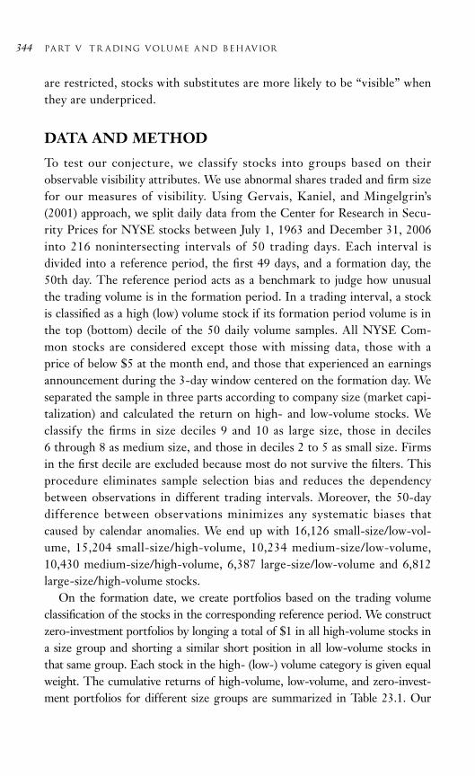
are restricted, stocks with substitutes are more likely to be “visible” whenthey are underpriced.
DATA AND METHOD
To test our conjecture, we classify stocks into groups based on theirobservable visibility attributes. We use abnormal shares traded and firm sizefor our measures of visibility. Using Gervais, Kaniel, and Mingelgrin’s(2001) approach, we split daily data from the Center for Research in Secu-rity Prices for NYSE stocks between July 1, 1963 and December 31, 2006into 216 nonintersecting intervals of 50 trading days. Each interval isdivided into a reference period, the first 49 days, and a formation day, the50th day. The reference period acts as a benchmark to judge how unusualthe trading volume is in the formation period. In a trading interval, a stockis classified as a high (low) volume stock if its formation period volume is inthe top (bottom) decile of the 50 daily volume samples. All NYSE Com-mon stocks are considered except those with missing data, those with aprice of below $5 at the month end, and those that experienced an earningsannouncement during the 3-day window centered on the formation day. Weseparated the sample in three parts according to company size (market capi-talization) and calculated the return on high- and low-volume stocks. Weclassify the firms in size deciles 9 and 10 as large size, those in deciles 6 through 8 as medium size, and those in deciles 2 to 5 as small size. Firmsin the first decile are excluded because most do not survive the filters. Thisprocedure eliminates sample selection bias and reduces the dependencybetween observations in different trading intervals. Moreover, the 50-daydifference between observations minimizes any systematic biases thatcaused by calendar anomalies. We end up with 16,126 small-size/low-vol-ume, 15,204 small-size/high-volume, 10,234 medium-size/low-volume,10,430 medium-size/high-volume, 6,387 large-size/low-volume and 6,812large-size/high-volume stocks.
On the formation date, we create portfolios based on the trading volumeclassification of the stocks in the corresponding reference period. We constructzero-investment portfolios by longing a total of $1 in all high-volume stocks ina size group and shorting a similar short position in all low-volume stocks inthat same group. Each stock in the high- (low-) volume category is given equalweight. The cumulative returns of high-volume, low-volume, and zero-invest-ment portfolios for different size groups are summarized in Table 23.1. Our
344 Part V TR ADING VOLUME A ND BEHAVIOR
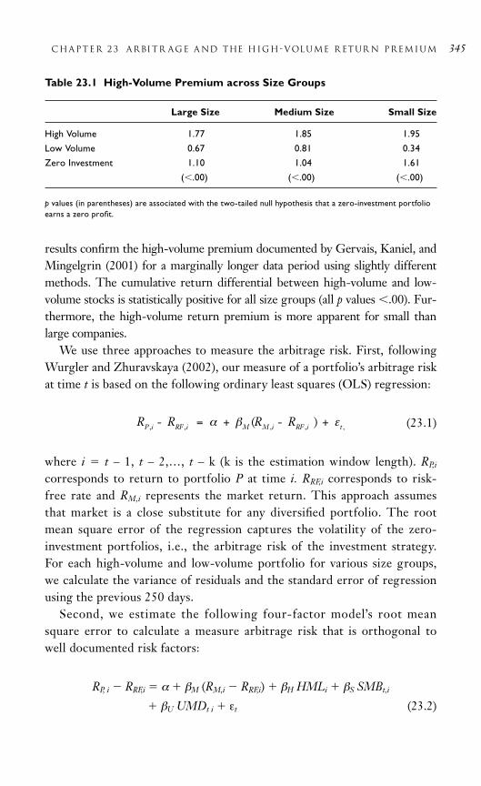
results confirm the high-volume premium documented by Gervais, Kaniel, andMingelgrin (2001) for a marginally longer data period using slightly differentmethods. The cumulative return differential between high-volume and low-volume stocks is statistically positive for all size groups (all p values .00). Fur-thermore, the high-volume return premium is more apparent for small thanlarge companies.
We use three approaches to measure the arbitrage risk. First, followingWurgler and Zhuravskaya (2002), our measure of a portfolio’s arbitrage riskat time t is based on the following ordinary least squares (OLS) regression:
(23.1)
where i t – 1, t – 2,…, t – k (k is the estimation window length). RP,i
corresponds to return to portfolio P at time i. RRF,i corresponds to risk-free rate and RM,i represents the market return. This approach assumesthat market is a close substitute for any diversified portfolio. The rootmean square error of the regression captures the volatility of the zero-investment portfolios, i.e., the arbitrage risk of the investment strategy.For each high-volume and low-volume portfolio for various size groups,we calculate the variance of residuals and the standard error of regressionusing the previous 250 days.
Second, we estimate the following four-factor model’s root meansquare error to calculate a measure arbitrage risk that is orthogonal towell documented risk factors:
RP, i RRF,i α βM (RM,i RRF,i) βH HMLi βS SMBt,i
βU UMDt i εt (23.2)
chapter 23 ARBITR AGE A ND THE HIGH-VOLUME R ETUR N Premium 345
Table 23.1 High-Volume Premium across Size Groups
Large Size Medium Size Small Size
High Volume 1.77 1.85 1.95
Low Volume 0.67 0.81 0.34
Zero Investment 1.10 1.04 1.61
(.00) (.00) (.00)
p values (in parentheses) are associated with the two-tailed null hypothesis that a zero-investment portfolioearns a zero profit.
R R R RP i RF i M M i RF i t, , , , ,- -( )= + +α β ε

where i t 1, t 2,…, t k and RP,i, RRFi, and RMi are previouslydefined. The purpose of adding other factors to Equation (23.1) is to capture the idiosyncratic risk that potentially creates major obstacles for thearbitrageur. We use book-to-market (high minus low, or HML) and size(small minus big, or SMB) to control for other sources of risk. HML andSMB are obtained from Kenneth French’s Web site. To control for possiblemomentum effects, we use the six value-weighted portfolios formed on sizeand prior 2- to 12-month returns. The portfolios are the intersections ofthe two portfolios formed on size and the three portfolios formed on priorreturn. The monthly size breakpoint is the median NYSE market equity.The monthly prior return breakpoints are the 30th and 70th NYSE percentiles. Momentum (up minus down, or UMD) is the average returnon the two high prior return portfolios minus the average return on thetwo low prior return portfolios. We do not include a liquidity variable inEquation (23.2) because Gervais, Kaniel, and Mingelgrin (2001) show thatliquidity is not an explanation for the high-volume return premium, but ourconclusions are not affected if we do.
Third, we create a fifth risk factor, LMS, which is the average returnon the portfolio that longs stocks in the top 20th percentile of arbitragerisk and shorts stocks in the lowest 20th percentile of arbitrage risk. Arbitrage risk for individual stocks is calculated based on OLS regressionfound in Equation (23.2). Sorting based on arbitrage risk is performedbefore the trading interval i; therefore, it is information available toinvestors before the portfolio formation period. If arbitrage risk is indeedhigher for less visible stocks, then inclusion of LMS (long minus short)should reduce or eliminate the alpha differential between most visible andless visible portfolios.
TESTS
The first implication of our conjecture is that arbitrage risk of visible stocksshould be lower than that of less visible ones. This translates into compar-ing arbitrage risk of high-volume stocks and low-volume stocks within thesame size group, and large-size and small-size firms within the same vol-ume group. In Table 23.2, we report that high-volume stocks have lowerarbitrage risk than low-volume stocks regardless of size firms (p values .01)and that large-size firms have lower arbitrage risk than small-size firms
346 Part V TR ADING VOLUME A ND BEHAVIOR

regardless of volume (p values .00). These results support the notion thatarbitrage risk may be capable of explaining the high-volume premium.
The p values (in parentheses) in Panel A show the results of the one-tailednull hypothesis that arbitrage risk of high-volume stocks is greater than thatof low-volume stocks. The p values (in parentheses) in Panel B show theresults of the one-tailed null hypothesis that arbitrage risk of large-size firmsis greater than that of small-size firms. We estimate Equation (23.2) with andwithout LMS for the more and less visible portfolios for all 216 20-day trad-ing intervals. The results are displayed in Table 23.3. These indicate thatfour-factor model alone cannot account for the return premium across high-and low-volume portfolios for all firm size groups. The alpha differences inall size groups are significant and positive. However, if the LMS factor isincluded in the four-factor model, the alpha difference is reduced substan-tially for all size groups. For large-size stocks the difference reduces from0.66 percent (p value .00) to 0.08 percent (p value .70). Adding LMS alsoreduces alpha for medium-size stocks. Alpha goes down from 1.31 percent (p value .00) to –0.03 percent (p value .58). In the small-size stocks, how-ever, inclusion of LMS does not eliminate the significance of alpha but alphais reduced from 2.05 percent ( p value .00) to 0.59 percent ( p value .09).
chapter 23 ARBITR AGE A ND THE HIGH-VOLUME R ETUR N Premium 347
Table 23.2 Arbitrage Risk Differences
Panel A.
High Volume, High Volume, High Volume Large Size/ Medium Size/ Small Size/
Low Volume, Low Volume, Low Volume,Large Size Medium Size Small Size
Risk Difference 0.483 0.220 0.116
(.00) (.00) (.01)
Panel B.
Large Size, Large Size,High Volume/ Low Volume/Small Size, Small Size,
High Volume Low Volume
Risk Difference 0.630 0.228
(.00) (.00)
p values (in parentheses) show the results of the one-tailed null hypothesis.

CONCLUSION
Our empirical evidence shows that arbitrage risk explains the premiumbetween high- and low-volume stocks. Our results confirm those ofGervais, Kaniel, and Minglegrin (2001) who document the existence of ahigh-volume premium. They are also consistent with the findings of Ang etal. (2006) who show that U.S. stocks with high lagged idiosyncratic volatilityearn very low future average returns. Moreover, our arbitrage interpretationof the visibility hypothesis complements Chan and Lakonishok (1993), whosuggest that buy decisions convey more information to the market than sell decisions because the latter are typically liquidity motivated. That theinformation effect on trading volume, however, is only part of the story.Investors, who provide the liquidity to other investors with limited invest-ment opportunity sets and who profit from any price discrepancy betweenmarket segments, care about the availability of perfect substitutes (arbitragerisk). Their demand for such assets increases the visibility of those assetsand forces other investors to consider them. When assets with low arbitragerisk are underpriced, increased visibility causes prices to increase andexpected returns to decrease. Overall, our results suggest that the visibilityand investor recognition related hypotheses should consider the arbitragerisk of the underlying asset because a shock to trading activity may signalpossible price corrections.
348 Part V TR ADING VOLUME A ND BEHAVIOR
Table 23.3 Four-Factor Alphas with and without LMS
Large-Size Medium-Size Small-Size
Without With Without With Without WithLMS LMS LMS LMS LMS LMS
High Volume 0.80 0.23 1.85 0.48 1.95 0.69
(.00) (.04) (.00) (.01) (.00) (.01)
Low Volume 0.14 0.15 0.54 0.51 0.10 0.10
(.08) (.06) (.04) (.01) (.15) (.07)
Alpha Difference 0.66 0.08 1.31 0.03 2.05 0.59
(.00) (.70) (.00) (.58) (.00) (.09)
LMSlong minus short.Two-tailed p values are in parentheses.

REFERENCES
Ang, A., Hodrick, R., Xing, Y., and Zhang, X. (2006) The Cross-section ofVolatility and Expected Returns. Journal of Finance, 61(2): 259–299.
Chan, L.K.C. and Lakonishok, J. (1993) Institutional Trades and IntradayStock Price Behavior. Journal of Financial Economics, 33(April):173–199.
French, K. http://mba.tuck.dartmouth.edu/pages/faculty/ken.french/data_library.html
Gervais, S., Kaniel, R., and Mingelgrin, D.H. (2001) The High-volumeReturn Premium. Journal of Finance, 56(3): 877–919.
Miller, E.M. (1977) Risk, Uncertainty, and Divergence of Opinion. Journalof Finance, 32(September): 1151–1168.
Wurgler, J. and Zhuravskaya, E. (2002) Does Arbitrage Flatten DemandCurves for Stocks? Journal of Business, 75( June): 583–608.
chapter 23 ARBITR AGE A ND THE HIGH-VOLUME R ETUR N Premium 349

This page intentionally left blank

351
24C H A P T E R
The Impact of Hard versus SoftInformation onTrading VolumeEvidence from Management Earnings Forecasts
Paul Brockman and Jim Cicon
ABSTRACT
We examine the impact of hard (quantitative) versus soft (qualitative)information on trading volume around the release of management earningsforecasts. We use textual analysis to identify and measure the level of twosoft information variables, Optimism and Certainty, in each forecast. We posit and confirm that soft information has a significant impact ontrading volume, even after controlling for the effect of hard information.In fact, we show that soft information explains more of the trading volumeimpact of management forecasts than hard information. Our empiricalresults contribute to the growing literature that examines the economicsignificance of qualitative information.

INTRODUCTION
In this chapter, we investigate how the release of management earningsforecasts impacts the announcing firm’s trading volume. Our main interestis to differentiate the impact of hard, or quantitative, information from theimpact of soft, or qualitative, information. Since a typical managementforecast announcement contains roughly 99 words for every one number,we expect that soft information (i.e., words instead of numbers) plays a significant role in providing relevant information to the market. The moreinformative the announcement, all else equal, the more abnormal tradingvolume the announcement will generate. We use textual analysis to identifyand measure the level of two specific soft information variables, Optimismand Certainty, in each management forecast. Our empirical results confirmthat soft information has a significant impact on trading volume, even aftercontrolling for the effect of hard information. More specifically, we findthat Optimism has a positive and significant impact on abnormal trading volume at the time of the forecast, while Certainty has a negative and significant impact on abnormal trading volume at the time of the forecast.These results suggest that qualitative information associated with greateroptimism increases investors’ propensity to trade, while qualitative infor-mation associated with greater certainty decreases their propensity totrade. In contrast, we find no significant relation between abnormal tradingand quantitative information.
Our chapter is motivated by combining the management forecast literature and the textual analysis literature. Previous studies show thatmanagement earnings forecasts contain substantial value-relevant infor-mation (Hirst, Koonce, and Venkataraman, 2008). Pownall, Wasley, andWaymire (1993) show that voluntary disclosures generate a significantprice effect at the time of the announcement. The market reassesses thefirm’s prospects as a result of the voluntary disclosure and adjusts its priceaccordingly. Coller and Yohn (1997) show that such announcements alsohave a significant impact on firm liquidity, and Baginski and Hassell(1990) find a significant impact on analyst revisions. Recent research byAboody and Kasznik (2000), Cheng and Lo (2006), and Brockman, Khurana, and Martin (2008) finds that managers exercise considerableleeway in the timing and content of their voluntary disclosures. For our purposes, the combination of value-relevant information and consid-erable managerial discretion offers an ideal setting in which to examine
352 Part V TR ADING VOLUME A ND BEHAVIOR

qualitative versus quantitative information. While required financialreports specify the form and content of disclosures, voluntary disclosures(e.g., management earnings forecasts) are open-ended. Managers not onlychoose whether or not to issue forecasts, they also choose the combina-tion of hard and soft information contained in their announcements.
There is a growing literature in accounting and finance that uses textualanalysis to examine the soft information content of firm announcements(e.g., Das and Chen, 2007; Tetlock, 2007; and Das, Martinez-Jerez, andTufano, 2005). Many, if not most, of these studies analyze the relationbetween soft information and the firm’s reported earnings (e.g., Li, 2006;Engelberg, 2007; Davis, Piger, and Sedor, 2007; Tetlock, Saar-Tsechansky,Macskassy, 2008; Demers and Vega, 2008). Demers and Vega (2008), forexample, investigate the price effect of hard versus soft information usingmore than 20,000 earnings announcements. Their results show that softinformation has a significant impact on stock prices at the time of the earnings announcement. Brockman and Cicon (2009) find similar, affirma-tive results for the role of soft information during the announcements ofmore than 15,000 management earnings forecasts.
The rest of this chapter proceeds as follows: we describe our data andmethods of analysis in this chapter’s second section. We present and analyzeour empirical findings in the third section of this chapter, and then providea brief conclusion in the final section.
DATA AND METHODOLOGY
Data
Our chapter analyzes the soft information found in the text of company-issued, guidance press releases. We use LexisNexis as the source of thesepress releases. Specif ically, we restrict our search to the LexisNexis “Company Press Releases” database and further limit our search to the following news providers: PR Newswire (US), Business Wire, and CanadaNewswire. Our timeframe is 1994 to 2007.
Our query analyzes the “subject” line and the “headline” of each candi-date press release. Starting with the subject line, we keep only those pressreleases which fall into the following categories: (“earnings preannounce-ments” or “earnings projections or forecasts”) and not (“interim financialresults”). We exclude the “interim financial results” hits because press
chapter 24 The Impact of Information on Trading Volume 353

releases in this category tend to originate from noncompany sources (e.g.,analyst commentary). We scan the headlines of the remaining documentsand retain only those that contain the following terms: (guidance OR forecast OR predict OR prediction OR projection OR forward OR futureOR expect OR expected OR expectation OR update OR anticipate OR reaffirm) AND ((cash W/S flow) OR earn OR earning OR share OR stockOR EPS OR fiscal OR price OR revenue OR results OR profit OR profitability OR targets OR growth OR raise OR lower OR upward ORupwardly OR downward OR downwardly). The AND connector betweenthe two groups of words means that one of the first group of words ANDone of the second group of words must appear in the headline in order forthe press release to be retained.
This LexisNexis search yields 74,603 candidate press releases, many ofwhich are duplicates and/or commentary by third parties subsequent tothe original press release. To ensure uniqueness and relevancy, we matchthe candidate press releases with the First Call “Company Issued Guide-lines” database. Since the 74,603 press releases downloaded from Lexis-Nexis are in PDF format, they are not readily identifiable by a machine.Therefore, we write custom software to scan and extract the ticker sym-bol and the announcement date from each press release. We retain onlythose press releases which match the First Call ticker symbol and whichoccur on the same day as the First Call guidance release. Where morethan one press release occurs on the same day for the same company, wekeep the earliest. We also discard press releases that do not contain atleast 100 words.
After these steps, we are left with 15,010 press releases. We randomlysample these press releases to ensure uniqueness and relevancy. We then run custom algorithms to clean up the press releases. We firstremove all punctuation. Hyphenated words are concatenated. Numericalterms are counted and then removed, with a record of their countretained. If tables are found, they are removed, although we keep recordof their presence with a dummy variable. Words which do not occur morethan two times in a given document are discarded. We truncate pressreleases which are longer than 750 words. This effectively removes company-description and safe-harbor paragraphs in the longer pressreleases. Shorter press releases do not typically contain these boilerplateparagraphs.
354 Part V TR ADING VOLUME A ND BEHAVIOR

Methodology
Our methodology analyzes each press release for the presence of semanticfeatures, specifically, for the presence of Optimism and Certainty. We baseour analysis on Diction, a language processing software package whichhas been used extensively in prior research to analyze political and eco-nomic speeches, corporate reports, and earnings announcements. Dictionanalyzes a document by counting the frequency of specific key words. It compares these counts to norms calculated from a broad sample ofEnglish text consist ing of 20,000 documents drawn from polit icalspeeches, newspaper editorials, business reports, scientific documents,telephone conversations, etc.
Diction defines Net Optimism (equivalent to our term Optimism) as lan-guage endorsing some person, group, concept or event, or highlighting theirposit ive accomplishments (Carroll, 2000). The program generates an aggregate standardized score for Optimism by counting words in definedcategories and combining the standardized scores for each category as shown
Optimism (praise satisfaction inspiration)
(blame hardship denial) (24.1)
Diction defines Certainty as language indicating resoluteness, inflexibility,completeness, and a tendency to speak ex cathedra. The program generatesan aggregate standardized score for Certainty by counting words in definedcategories and combining the standardized scores for each category as shown
Certainty (tenacity leveling collectives numerical_terms)
(ambivalence self_reference variety) (24.2)
These two semantic features, Net Optimism and Certainty serve as the softinformation variables in our chapter.
In addition to standardizing our qualitative information variables usingDiction’s out-of-sample mean and variance values, we replicate all empiricaltests using in-sample mean and variance values. We find no substantive difference between either approach and conclude that our empirical resultsand conclusions are not sensitive to the standardization procedure.
chapter 24 The Impact of Information on Trading Volume 355
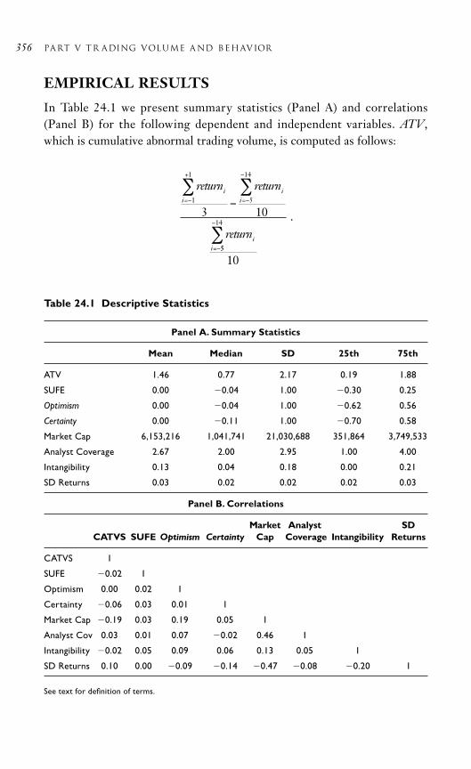
EMPIRICAL RESULTS
In Table 24.1 we present summary statistics (Panel A) and correlations(Panel B) for the following dependent and independent variables. ATV,which is cumulative abnormal trading volume, is computed as follows:
356 Part V TR ADING VOLUME A ND BEHAVIOR
return return
return
ii=
+
ii=
ii=
− −
−
−
∑ ∑−1
1
5
14
3 10
55
14
10
.−
∑
Table 24.1 Descriptive Statistics
Panel A. Summary Statistics
Mean Median SD 25th 75th
ATV 1.46 0.77 2.17 0.19 1.88
SUFE 0.00 0.04 1.00 0.30 0.25
Optimism 0.00 0.04 1.00 0.62 0.56
Certainty 0.00 0.11 1.00 0.70 0.58
Market Cap 6,153,216 1,041,741 21,030,688 351,864 3,749,533
Analyst Coverage 2.67 2.00 2.95 1.00 4.00
Intangibility 0.13 0.04 0.18 0.00 0.21
SD Returns 0.03 0.02 0.02 0.02 0.03
Panel B. Correlations
Market Analyst SDCATVS SUFE Optimism Certainty Cap Coverage Intangibility Returns
CATVS 1
SUFE 0.02 1
Optimism 0.00 0.02 1
Certainty 0.06 0.03 0.01 1
Market Cap 0.19 0.03 0.19 0.05 1
Analyst Cov 0.03 0.01 0.07 0.02 0.46 1
Intangibility 0.02 0.05 0.09 0.06 0.13 0.05 1
SD Returns 0.10 0.00 0.09 0.14 0.47 0.08 0.20 1
See text for definition of terms.

SUFE is the standardized unexpected earnings forecast. Optimism is “ameasure of language endorsing some person, group, concept or event, orhighlighting their positive entailments.” Certainty consists of words indicat-ing resoluteness, inflexibility, and completeness. Market cap is the naturallogarithm of the firms’ market capitalization. Analyst coverage is the numberof analysts covering firm j in quarter t. Intangibility is intangible assetsdivided by total assets. Standard deviation (SD) of returns is the standarddeviation of returns from 30 days to 7 days from the announcementdate. The sample period spans 1994 to 2007 and includes those firms whichappeared in the First Call company-issued, guidelines database and forwhich a matching company press release was found in LexisNexis for a totalof 14,938 company-issued, guidance press releases.
Our dependent variable, ATV, is measure of abnormal trading volumethat compares trading volume around management guidance announce-ments with trading volume in the preannouncement period. ATV is definedas follows:
(24.3)
Our main treatment variables include a quantitative variable, SUFE, andtwo qualitative variables, Optimism and Certainty. SUFE is the standardizedunexpected earnings forecast. We construct SUFE by subtracting the man-agement earnings forecast of firm j for time period t from the firm’s actual(reported) earnings in time period t 1. This difference is used as theunexpected component in the manager’s forecast. Lastly, we calculate SUFEby subtracting the sample mean and dividing by the sample standard devia-tion. Our first qualitative variable, Optimism, is “a measure of languageendorsing some person, group, concept or event, or highlighting their posi-tive entailments.” Our second qualitative variable, Certainty, consists ofwords indicating resoluteness, inflexibility, and completeness.
Our control variables include market capitalization, analyst coverage,intangibility, and standard deviation of returns. MktCap is the natural
chapter 24 The Impact of Information on Trading Volume 357
return return
return
ii=
+
ii=
ii=
− −
−
−
∑ ∑−1
1
5
14
3 10
55
14
10
−
∑

logarithm of the firms’ market capitalization. Analyst coverage is the numberof analysts covering firm j in quarter t. Intangibility is intangible assetsdivided by total assets. StdDevRet is the standard deviation of returns from30 days to 7 days from the announcement date. Our sample period isfrom 1994 to 2007. The sample includes those firms which appeared in theFirst Call company-issued, guidelines database and for which a matchingcompany press release was found in LexisNexis for a total of 14,938 company-issued, guidance press releases.
We present our baseline regression results in Table 24.2. We estimatethe following regression:
ATVi β0 β1 SUFEi β2 Optimismi β3 Certaintyi β4 MktCapi
β5 Analysti β6 Intangibilityi β7 StdDevReti εi (24.4)
where all variables are defined above. The sample period spans 1994 to 2007and includes those firms which appeared in the First Call company-issued,guidelines database and for which a matching company press release wasfound in LexisNexis for a total of 14,938 company-issued, guidance pressreleases. We control for industry effects, not shown. Our main variables ofinterest are the treatment variables SUFE, Optimism, and Certainty. Thecoefficient on SUFE is negative and insignificant, suggesting that the unex-pected component of guidance forecasts does not have a significant impacton trading volume. In contrast, the coefficients for both qualitative variablesare significant. The coefficient on Optimism is positive and significant.
358 Part V TR ADING VOLUME A ND BEHAVIOR
Table 24.2 Baseline Regression—Impact of Soft Information on Trading Volume
Coefficient t stat p value
SUFE 0.0246 1.399 0.1619
Optimism 0.0804 4.458 0.0000****
Certainty 0.0977 5.454 0.0000****
MktCap 0.5798 24.92 0.0000****
Analyst Coverage 0.3125 15.499 0.0000****
Intangibility 0.0441 2.326 0.0200**
SD Returns 0.1025 4.804 0.0000****
Adjusted R2 6.32%
**** denotes significance at 0.1%, *** at 1%, ** at 5%, and * at 10%.

This result means that the more optimistic the language contained in themanagement guidance, the larger the increase in abnormal trading. Thecoefficient on Certainty is negative and significant, suggesting that the morecertain the language contained in the management guidance, the smaller theincrease in abnormal trading. Overall, these findings show that trading volume is very sensitive to soft information. All else equal, more optimistlanguage increases trading volume and more certain language decreasestrading volume.
The coefficients on the control variables in regression in Equation (24.3)show that abnormal trading increases with analyst coverage and decreases withmarket capitalization, intangibility, and the standard deviation of returns.
In Table 24.3, we estimate the following augmented regression modelthat includes interaction terms between the soft and hard variables:
(24.5)
where all variables are defined above. The sample period spans 1994 to 2007and includes those firms which appeared in the First Call company-issued,guidelines database and for which a matching company press release wasfound in LexisNexis for a total of 14,938 company-issued, guidance press
chapter 24 The Impact of Information on Trading Volume 359
ATV = + SUFE + Optimism + Certainty +i i i iβ β β β
β0 1 2 3
4SSUFE Optimism + SUFE Certainty +MktCa
i i i i∗ ∗β
β5
6 pp + Analyst + Intangibility + StdDevReti i iβ β β7 8 9 ii i+ ε
Table 24.3 Substitution/Complementary Effects of SoftInformation for Earnings Forecast Information
Coefficient t stat p value
SUFEOptimism 0.0062 0.416 0.6771
SUFECertainty 0.0201 1.127 0.2597
SUFE 0.0229 1.296 0.1951
Optimism 0.0805 4.461 0.0000****
Certainty 0.0981 5.473 0.0000****
MktCap 0.5792 24.9 0.0000****
Analyst Coverage 0.3125 15.5 0.0000****
Intangibility 0.0437 2.302 0.0213**
SD Returns 0.1018 4.767 0.0000****
Adj R^2 6.32%
**** denotes significance at 0.1%, *** at 1%, ** at 5%, and * at 10%.

releases. We control for industry effects, not shown. We are primarily inter-ested in the coefficients on the two interaction terms, SUFEOptimism andSUFECertainty. These coefficients allow us to test if there are significantinteraction effects between hard and soft information (e.g., the full impact ofOptimism on ATV is composed of a direct effect (measured by β2) and anindirect or interaction effect (measured by β4SUFE). The indirect effectstell us if soft and hard information behave as complements or substitutes toone another. Our results in Table 24.3 show that there are no significantinteraction effects for either soft variable. Both interaction coefficients arepositive but insignificant. This finding suggests that the impact of Optimismand Certainty on abnormal trading volume is a direct effect; that is, theimpact is not dependent on the level of SUFE.
We examine additional interaction effects in Table 24.4. We estimate thefollowing four regressions with interaction terms for each of our controlvariables (included one at a time):
ATVi β0 β1 SUFEi β2 Optimismi β3 Certaintyi β4 ControlVari *Optimismi β5 ControlVari * Certaintyi β6 MktCapi β7 Analysti
β8 Intangibilityi β9 StdDevReti εi (24.6)
where all variables are defined above, and the term ControlVar stands for eitherMktCap, Analyst, Intangibility, or StdDevRet, depending on the regression.The sample period spans 1994 to 2007 and includes those firms whichappeared in the First Call company-issued, guidelines database and for which amatching company press release was found in LexisNexis for a total of 14,938company-issued, guidance press releases. We control for industry effects, notshown. We report the results of interacting MktCap with our soft informationvariables in Panel A. The interaction between Optimism and MktCap is nega-tive and insignificant, while the interaction between Certainty and MktCap ispositive and significant. This latter result suggests that Certainty has a largerimpact on the trading volume of large firms than small firms. We find a simi-lar interaction effect between Certainty and Intangibility in Panel C. That is,the interaction between Optimism and Intangibility is negative and insignifi-cant, while the interaction between Certainty and Intangibility is positive andsignificant. Certainty has a larger impact on the trading volume of firms withmore intangible assets. In contrast, we find no significant interaction effectsfor Analyst Coverage and StDevRet in Panels B and D, respectively.
360 Part V TR ADING VOLUME A ND BEHAVIOR

CONCLUSION
The primary objective of this chapter is to examine the impact of hard(quantitative) versus soft (qualitative) information on trading volumearound the release of management earnings forecasts. Our chapter is moti-vated by the growing literature that links soft information to market reac-tions, as well as previous studies showing that management forecastscontain value-relevant information. We use textual analysis to identify andmeasure the level of two soft information variables, Optimism andCertainty. We hypothesize that these soft information variables will have a
chapter 24 The Impact of Information on Trading Volume 361
Table 24.4 Substitution/Complementary Effects of Soft Information for Other Firm Characteristics
Panel A. Market Capitalization Panel B. Analyst Coverage
Coefficient Coefficient
MktCapOptimism 0.0119 0.0242
MktCapCertainty 0.0763**** 0.0237
SUFE 0.0236 0.0251
Optimism 0.0829**** 0.0784****
Certainty 0.1100**** 0.0963****
MktCap 0.5703**** 0.5804****
Analyst Coverage 0.3117**** 0.3119****
Intangibility 0.0442** 0.0449**
SD Returns 0.1074**** 0.1022****
Adjusted R2 6.43% 6.33%
Panel D. Standard Panel C. Intangibility Deviation of Returns
Coefficient Coefficient
IntangibilityOptimism 0.0247 0.0116
IntangibilityCertainty 0.0466*** 0.0210
SUFE 0.0243 0.0249
Optimism 0.0791**** 0.0808****
Certainty 0.1004**** 0.1010****
MktCap 0.5803**** 0.5797****
Analyst Coverage 0.3141**** 0.3127****
Intangibility 0.0434** 0.0436**
SD Returns 0.1052**** 0.1074****
Adjusted R2 6.37% 6.32%
**** denotes significance at 0.1%, *** at 1%, ** at 5%, and * at 10%.
significant impact on trading volume at the time of earnings guidanceannouncements. Our empirical results confirm this hypothesis. We find apositive and significant relation between abnormal trading volume and Optimism, and a negative and significant relation between abnormal tradingvolume and Certainty. In contrast, we do not find a significant relationbetween abnormal trading volume and our measure of hard information,the standardized unexpected earnings forecast. Overall, our chapter con-tributes to the growing literature that examines the economic significanceof qualitative information.
REFERENCES
Aboody, D. and Kasznik, R. (2000) CEO Stock Option Awards and theTiming of Voluntary Corporate Disclosures. Journal of Accounting andEconomics, 29(1): 73–100.
Baginski, S. and Hassell, J. (1990) The Market Interpretation of Manage-ment Earnings Forecasts as a Predictor of Subsequent Financial Analyst Forecast Revision. The Accounting Review, 65(1): 175–190.
Brockman, P. and Cicon, J. (2009) The Information Content of ManagementEarnings Forecasts: An Analysis of Hard versus Soft Data. Workingpaper, University of Missouri, Columbia, MO.
Brockman, P., Khurana, I., and X. Martin. (2008) Voluntary Disclosuresaround Share Repurchases. Journal of Financial Economics, 89(1):175–191.
Cheng, Q. and Lo, K. (2006) Insider Trading and Voluntary Disclosures.Journal of Accounting Research, 44(5): 815–848.
Coller, M. and Yohn, T. (1997) Management Forecasts and InformationAsymmetry: An Examination of Bid-Ask Spreads. Journal of AccountingResearch, 35(2): 181–191.
Das, S. and Chen, M. (2007) Yahoo! For Amazon: Sentiment Extractionfrom Small Talk on the Web. Management Science, 53(9): 1375–1388.
Das, S., Martinez-Jerez, A., and Tufano, P. (2005) E-information: A ClinicalStudy of Investor Discussion and Sentiment. Financial Management,34(3): 103–137.
Davis, A., Piger, J., and Sedor, L. (2007) Beyond the Numbers: Managers’Use of Optimistic and Pessimistic Tone in Earnings Press Releases.Working paper, University of Washington, Seattle, WA.
362 Part V TR ADING VOLUME A ND BEHAVIOR

Demers, E. and Vega, C. (2008) Soft Information in Earnings Announce-ments: News or Noise? Working paper, INSEAD, Fontainebleau,France.
Engelberg, J. (2007) Costly Information Processing: Evidence from Earn-ings Announcements. Working paper, Northwestern Universit y,Evanston, IL.
Hirst, E., Koonce, L., and Venkataraman, S. (2008) Management EarningsForecasts: A Review and Framework. Accounting Horizons, 22(3):315–338.
Li, F. (2006) Do Stock Market Investors Understand the Risk Sentiment ofCorporate Annual Reports? Working paper, University of Michigan,Ann Arbor, MI.
Pownall, G., Wasley, C., and Waymire, G. (1993) The Stock Price Effects ofAlternative Types of Management Earnings Forecasts. The AccountingReview, 68(October): 896–912.
Tetlock, P. (2007) Giving Content to Investor Sentiment: The Role ofMedia in the Stock Market. Journal of Finance, 62(3): 1139–1168.
Tetlock, P., Saar-Tsechansky, M., and Macskassy, S. (2008) More than Words:Quantifying Language to Measure Firms’ Fundamentals. Journal ofFinance, 63(3): 1437–1467.
chapter 24 The Impact of Information on Trading Volume 363

This page intentionally left blank

365
25C H A P T E R
Modeling Bubblesand Anti-Bubbles in Bear MarketsA Medium-Term Trading Analysis
Dean Fantazzini
ABSTRACT
The current volatile market situation with sudden changes seems all butpredictable. However, some recent works have suggested that, prior tocrashes as well as after crashes, financial asset prices can be characterized bya power law acceleration decorated with log-periodic oscillations. Johansenand Sornette (1999) and Zhou and Sornette (2005) show that these pro-cesses take place because of the traders’ herding behavior which can pro-gressively occur and strengthen itself into “bullish” or “bearish” marketphases, thus forming bubbles and anti-bubbles, respectively. We brieflyreview the theory behind this kind of modeling and we perform an empiri-cal analysis with different world stock market indexes to verify whether amedium-term trading strategy based on this modeling can outperform sim-ple buy-and-hold or short-and-hold strategies.
INTRODUCTION
The current global financial crisis which began in 2007 has probably becomeone of the most interesting examples of how the bursting of a bubble can bedealt with by creating new bubbles. While this consideration may be seen at
first a little bit strong (but not new; see, e.g., Sornette and Woodard, 2009,and references therein), it has been recently confirmed by Lou Jiwei, thechairman of the $298 billion sovereign wealth fund named China Invest-ment Corporation (CIC). This fund was created in 2007 for managing partof the People’s Republic of China’s foreign exchange reserves, with the spe-cific goal to generate higher returns through advanced asset managementtechniques. On August 28, 2009, Lou told reporters on the sidelines of aforum organized by the Washington-based Brookings Institution and theChinese Economists 50 Forum, a Beijing think tank, that “both China andAmerica are addressing bubbles by creating more bubbles and we’re just taking advantage of that. So we can’t lose.” Moreover, asked whether CICwould be a keen buyer in the United States, Lou said, “CIC can buy anywhere in the world, but it cannot avoid buying U.S. assets because theU.S. economy and capital markets are so large.” Besides, Lou added that “CIC was building a broad investment portfolio that includes productsdesigned to generate both alpha and beta; to hedge against both inflation anddeflation; and to provide guaranteed returns in the event of a new crisis.”See the full Reuters article by Zhou Xin and Alan Wheatley (2009) athttp://www.reuters.com/article/ousiv/idUSTRE57S0D420090829 for moredetails. Clearly, the previous comments highlight how important is to havean appropriate model for bubbles and so-called anti-bubbles, which refer tothe period following the burst of a bubble.
A model which has quickly gained a lot of attention among practitionersand academics due to many successful predictions is the so-called log peri-odic power law (LPPL) model proposed by Sornette, Johansen, andBouchaud (1996), Sornette and Johansen (1997), Johansen, Ledoit, and Sornette (2000), and Sornette (2003). These authors suggested that, priorto crashes, the mean function of an index price time-series is characterizedby a power law acceleration decorated with log-periodic oscillations, leadingto a finite-time singularity that describes the onset of the market crash.Within this model, this behavior would hold for months and years inadvance, allowing the anticipation of the crash from the log-periodic oscil-lations exhibited by the prices. The underlying hypothesis of this model isthe existence of a growing cooperative action of the market traders due toan imitative behavior among them. Particularly, Johansen, Ledoit, and Sornette (2000) put forward the idea that stock market crashes are causedby the slow build up of long-range correlations leading to a collapse of the
366 PART V TR ADING VOLUME A ND BEHAVIOR

stock market in one critical instant. For a recent review of the theoreticalframework of the log-periodic model and a compilation of empirical evidences, see Sornette (2003). Johansen and Sornette (1999) and Zhou andSornette (2005) addressed the problem of whether there exist critical timestc at which the market peaks and then follows a power law decrease withdecelerating log-periodic oscillations; in the latter case we have a so calledanti-bubble. Johansen and Sornette (1999) and Zhou and Sornette (2005)showed that the traders’ herding behavior can progressively occur andstrengthen itself also in “bearish” decreasing market phases, thus forminganti-bubbles with decelerating market devaluations following market peaks.
What we do in this chapter is to briefly review the theory behind thiskind of modeling and perform an empirical analysis with different worldstock market indexes to verify whether a medium-term trading strategybased on this modeling can outperform simple buy-and-hold or short-and-hold strategies.
The rest of the chapter is organized as follows. In the second section ofthis chapter, we review the log-periodic models for bubble and anti-bubblemodeling, and in the third section we show an empirical application withworld stock market indexes. We perform an out-of-sample analysis in thischapter’s fourth section, and the fifth section briefly concludes.
LOG-PERIODIC MODELS: A REVIEW
Johansen, Ledoit, and Sornette (2000) considered an ideal market in a sce-nario purely speculative that does not pay dividends. For simplicity, inter-est rates, risk aversion, and market liquidity constraints are ignored. Inthis scenario, there is at least a rational agent, risk neutral and withrational expectations. Given these assumptions, the price at time t, p(t), offinancial assets should follow a martingale stochastic process. If we con-sider that there is a nonzero probability of a crash taking place, formally,we can define a counter function for the occurrence of the crash, given bya step function j(t) Ω(t–tc) whose value is zero before the crash and oneafter the occurrence of the crash at the time tc. Since tc is unknown, it isdescribed by a stochastic variable subject to a probability density functionq(t) and a cumulative distribution function Q(t)
q(t′)dt′. If we define
the hazard rate h(t) as the probability per unit of time of the crash takingplace in the next instant, given that it has not yet occurred, that is
chapter 25 MODELING BUBBLES A ND A NTI-BUBBLES IN BEAR MARKETS 367

h(t) q(t)/[1 – Q(t)], then the martingale condition implies that theexpected price rise must be just sufficient to compensate for the knownrisk of a crash. As a consequence, the dynamics of the price is given by
dp k p(t) h(t) dt (25.1)
where dp is the price change over the time interval dt, while k ∈ (0,1) is thefixed proportion by which the price is expected to drop, and we remark thatall the terms on the right hand side of Equation (25.1) are positive. If wereorder the previous equation, we have dp/p(t) k h(t) dt, and after inte-grating we get
(25.2)
Equation (25.2) shows an interesting result: the higher the probability ofa crash (given it has not yet taken place), the faster the price growth has tobe. Intuitively, investors must be compensated with higher returns for therisk of higher losses. The significant deviation of prices in relation to itsfundamental value for long periods of time is an issue still being debated infinancial literature and in particular has been examined by Blanchard(1979), who introduced a model for bubble with rational expectations.
This effect is not particular to the specific dynamics described by Equa-tion (25.2). If we alternatively assume that during the crash the price drops afixed percentage k ∈ (0,1) of the speculative price increase in relation to a certainfundamental value p*, then the dynamics of the price before the of the crashis given by
dp k [p(t) – p*] h(t) dt (25.3)
If we integrate Equation (25.3) and assume that p(t) – p(t0) p(t0) – p*,we have
(25.4)
368 PART V TR ADING VOLUME A ND BEHAVIOR
ln ( ) ( ) ( ) ( )exp ( )p t k h t dt p t p t k h t dt
t
= ′ ′ = ′ ′∫0
0or ttt
t
0
∫⎛
⎝⎜⎜
⎞
⎠⎟⎟
p t p t k p t p h t dt p t kt
t
( ) ( ) ( ( ) *) ( ) ( ) (= + ′ − ′ ′ = +∫0 0
0
pp t p k h t dtt
t
( ) *) ( )0
0
− ′ ′∫

The model therefore does not impose any constraint on the dimension ofthe crash: if we assume that it is proportional to the current market price,then we have to deal with the natural logarithm of prices, as shown byEquation (25.1) and Equation (25.2). Instead, if we assume that the ampli-tude of the crash is a fraction of the gain observed during the bubble, thenthe variable to consider is the price in levels, according to Equation (25.3)and Equation (25.4). In both cases, conditionally on staying in a bubblewith no crash occurrence, the asset price should grow rationally to com-pensate buyers for taking the risk of a market crash.
However, it is important to remark that there is a small probability thatthe system, starting from time t, will reach the end of the bubble withoutthe occurrence of a crash
(25.5)
This residual probability is crucial for the consistency of the modelbecause, otherwise, the agents would anticipate the crash and quit the market.
According to Equation (25.2) or Equation (25.4), the temporal evolutionof prices during the bubble depends on the hazard rate h(t), whose determi-nation is developed by using models coming from statistical physics.
Johansen, Ledoit, and Sornette (2000) propose a model where eachtrader i can be in one of two states, either bull (si 1) or bear (si 1),while at the next time step the state of trader is determined by the followingformula:
(25.6)
where K is an imitation factor, N(i) is the group of neighboring traders whoinfluence trader i, σ is the tendency towards idiosyncratic behavior amongstall traders, whereas εi is a random draw from a standard normal distribu-tion. Moreover, they assume that during a bubble the value of K increasesuntil it reaches a critical value Kc, and this increase is developed such that Kc – K(t) depends on the time span tc – t. As a consequence, the hazard rateh varies in the same way as K /Kc.
chapter 25 MODELING BUBBLES A ND A NTI-BUBBLES IN BEAR MARKETS 369
1− ∫ h t dtt
tc
( )
s sign K si j ij N i
= +⎛
⎝⎜⎜
⎞
⎠⎟⎟
∈
∑ σε( )
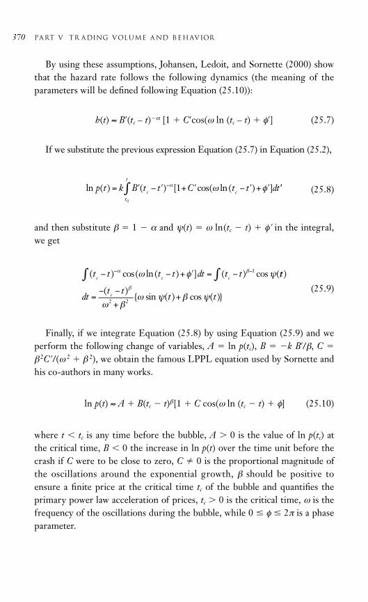
By using these assumptions, Johansen, Ledoit, and Sornette (2000) showthat the hazard rate follows the following dynamics (the meaning of theparameters will be defined following Equation (25.10)):
h(t) ≈ B′(tc – t)α [1 C′cos(ω ln (tc – t) φ′] (25.7)
If we substitute the previous expression Equation (25.7) in Equation (25.2),
(25.8)
and then substitute β 1 α and ψ(t) ω ln(tc t) φ′ in the integral,we get
(25.9)
Finally, if we integrate Equation (25.8) by using Equation (25.9) and weperform the following change of variables, A ln p(tc), B k B′/β, C
β2C′/(ω 2 β 2), we obtain the famous LPPL equation used by Sornette andhis co-authors in many works.
ln p(t) ≈ A B(tc t)β[1 C cos(ω ln (tc t) φ] (25.10)
where t tc is any time before the bubble, A 0 is the value of ln p(tc) atthe critical time, B 0 the increase in ln p(t) over the time unit before thecrash if C were to be close to zero, C 0 is the proportional magnitude ofthe oscillations around the exponential growth, β should be positive toensure a finite price at the critical time tc of the bubble and quantifies theprimary power law acceleration of prices, tc 0 is the critical time, ω is thefrequency of the oscillations during the bubble, while 0 φ 2π is a phaseparameter.
370 PART V TR ADING VOLUME A ND BEHAVIOR
ln ( ) ( ) [ cos( ln ( ) ]p t k B t t C t t dc c= ′ − ′ + ′ − ′ + ′−α ω φ1 ′′∫ tt
t
0
( ) cos( ln ( ) ] ( ) cos (t t t t dt t tc c c− − + ′ = −− −∫ α βω φ ψ1 tt
dtt t
t tc
)
( ) sin ( ) cos ( )
∫
=− −
++
β
ω βω ψ β ψ
2 2

A similar procedure can be followed in case of Equation (25.4) and we would obtain an Equation very close to Equation (25.10), with theonly difference being the dependent variable given by the price in levelsinstead of the log price. The two crucial parameters in this specificationare β and ω; Johansen, Ledoit, and Sornette (2000), Sornette (2003), andreferences therein show that for the underlying mechanism to be validatedβ should be included in 0 β 1, while 4 ω 15. By using a largecollection of empirical evidence they found that β 0.33 0.18, while ω 6.36 1.56.
However, we want to remark that even though the specific underlyingtheoretical mechanism is not always validated (for example, it is not un-usual to find β 1), the LPPL with suitable parameters can provide agood fit to the examined bubble and help forecasting its future develop-ment. For more discussion about these issues as well as recent criticism, werefer the interested reader to Chang and Feigenbaum (2006) and Lin Ren,and Sornette (2010).
Johansen and Sornette (1999) and Zhou and Sornette (2005) examinedthe problem of whether the cooperative herding behavior of traders mightalso produce market evolutions that are symmetric to the accelerating spec-ulative bubbles often ending in crashes. They show that there seems to existcritical times tc at which the market peaks and then decreases following apower law with decelerating log-periodic oscillations; in the latter case wehave a so called anti-bubble. Therefore, given this symmetric nature ofanti-bubbles, a straightforward way to model them is by simply invertingthe term (tc t) in Equation (25.10).
ln p(t) ≈ A B(t tc)β [1 C cos(ω ln (t tc) φ] (25.11)
p(t) ≈ A B(t tc)β [1 C cos(ω ln (t tc) φ] (25.12)
if we use log prices or if we use price in levels, instead. Clearly, in thelatter case the values of the parameters A, B, C will be much differentwith respect to the corresponding ones obtained with Equation (25.11),while the parameters β, ω, and ϕ should have similar values in both thetwo specifications.
Due to space limits, we do not discuss here about model estimation: weonly remark that even though Equations (25.10), (25.11), and (25.12) can
chapter 25 MODELING BUBBLES A ND A NTI-BUBBLES IN BEAR MARKETS 371

be estimated by nonlinear least squares, these formula are highly nonlinearand local maxima are very easy to find. Therefore, Johansen, Ledoit, andSornette (2000) proposed a multistep procedure involving grid searches as well as the use of the Nelder-Mead simplex search. The estimation ofsuch models is not an easy task and the author of this chapter has used anew alternative method which seems to be very promising, but still needsmore beta-testing and future work. We leave this as avenue for futureresearch. Anyway, some computational tips will be described in the nextsection.
EMPIRICAL ANALYSIS WITH WORLD STOCK MARKET INDEXES
We report below the in-sample estimation results for Equations (25.11)and (25.12) for the most important world stock market indexes (the timet is converted in units of one year, 1/365 0.002739. . .). We found thatestimating LPPL for anti-bubbles was much easier when using a single-digit time variable t, for example “9”, instead of a triple-digit variable“2009.” Furthermore, estimating models with log-prices was much simpler than models with prince in levels: in the latter case a more care-ful choice of the starting values has to be made. Interestingly, we noticedthat if a time series was clearly NOT following a LPPL anti-bubble pattern,then the model using prices in levels was never able to reach numerical convergence, even after a careful choice of starting values. Instead, themodel using log-prices always converged but with the parameters β 1 and ω 4.
To increase estimation efficiency and to reduce the parameter space, weused here for the first time the following computational solution: differ-ently from bubbles, when we work with anti-bubbles we do know the date ofthe global maxima as well as the corresponding price. As a consequence,the parameter tc need not be estimated and can be fixed a priori. The samesolution can be implemented for A, but we found it less crucial, from anumerical point of view, than fixing tc. The estimated parameters for the model with log-prices in Equation (25.11) and prices in levels inEquation (25.12), as well as the fitted series are reported below for eachstock market index.
372 PART V TR ADING VOLUME A ND BEHAVIOR

German DAX Index (12/12/2007–08/20/2009)
chapter 25 MODELING BUBBLES A ND A NTI-BUBBLES IN BEAR MARKETS 373
9000
8000
6000
7000
5000
4000
3000
12/1
2/07
12/0
1/08
12/0
2/08
12/0
3/08
12/0
4/08
12/0
5/08
12/0
6/08
12/0
7/08
12/0
8/08
12/0
9/08
12/1
0/08
12/1
1/08
12/1
2/08
12/0
1/09
12/0
2/09
12/0
3/09
12/0
4/09
12/0
5/09
12/0
6/09
12/0
7/09
12/0
8/09
Log-pricesDow Prices in levels
Figure 25.1 DAX Index and Fitted Series from Model 25.11 and Model 25.12
Table 25.1 DAX, Fitted Parameters Model 25.11and Model 25.12
Prices in Levels Log-Prices
A 7,644.31 8.90
B 2,078.80 0.30
Beta 0.72 1.15
C 998.83 0.19
Omega 4.08 4.49
Phi 3.02 3.07

U.S. Dow Jones Index (10/09/2007–08/20/2009)
374 PART V TR ADING VOLUME A ND BEHAVIOR
15000
14000
13000
10000
9000
12000
11000
8000
7000
6000
09/10/07
09/11/07
09/12/07
09/01/08
09/02/08
09/03/08
09/04/08
09/05/08
09/06/08
09/07/08
09/08/08
09/09/08
09/10/08
09/11/08
09/12/08
09/01/09
09/02/09
09/03/09
09/04/09
09/05/09
09/06/09
09/07/09
09/08/09
Log-pricesDow Prices in levels
Figure 25.2 Dow Jones Index and Fitted Series from Model 25.11 andModel 25.12
Table 25.2 Dow Jones, Fitted Parameters Model25.11 and Model 25.12
Prices in Levels Log-Prices
A 13,659.53 9.51
B –3,052.60 –0.24
Beta 1.05 1.35
C 1,388.09 0.14
Omega 4.82 4.97
Phi 2.24 2.22

(Figures for the market indexes in Tables 25.3 to 25.7 are not reporteddue to space limits).
British FTSE Index (10/12/2007–08/20/2009)
chapter 25 MODELING BUBBLES A ND A NTI-BUBBLES IN BEAR MARKETS 375
Table 25.4 KOSPI, Fitted Parameters Model 25.11and Model 25.12
Prices in Levels Log-prices
A 1,975.55 7.57
B –510.36 –0.29
Beta 0.68 0.92
C 292.32 0.21
Omega 4.65 4.82
Phi 2.84 2.86
Table 25.3 FTSE, Fitted Parameters Model 25.11and Model 25.12
Prices in Levels Log-Prices
A 13659.53 9.51
B –3052.60 –0.24
Beta 1.05 1.35
C 1,388.09 0.14
Omega 4.82 4.97
Phi 2.24 2.22
Korean KOSPI Index (10/31/2007–08/20/2009)
Italian MIBTel Index (10/12/2007–08/20/2009)
Table 25.5 MIBTel, Fitted Parameters Model25.11 and Model 25.12
Prices in Levels Log-Prices
A 40,991.96 10.59
B –15,392.28 –0.45
Beta 0.82 1.14
C 3,924.46 0.17
Omega 5.16 5.37
Phi 2.31 2.19

Japanese Nikkei Index (07/09/2007–08/20/2009)
376 PART V TR ADING VOLUME A ND BEHAVIOR
Table 25.6 Nikkei, Fitted Parameters Model 25.11and Model 25.12
Prices in Levels Log-Prices
A 17,617.62 9.76
B –5,301.38 –0.35
Beta 0.90 1.19
C 1,525.32 0.14
Omega 7.58 7.61
Phi 0.35 0.33
Table 25.7 Bovespa, Fitted Parameters Model25.11 and Model 25.12
Prices in Levels Log-Prices
A Not converged 11.09
B Not converged –1.31
Beta Not converged 1.65
C Not converged –1.18
Omega Not converged 2.21
Phi Not converged 2.66
Brazilian Bovespa Index (05/28/2008–08/20/2009)
U.S. S&P 500 Index (10/09/2007–08/20/2009)
Table 25.8 S&P 500, Fitted Parameters Model25.11 and Model 25.12
Prices in Levels Log-Prices
A 1518.69 7.31
B –375.51 –0.28
Beta 1.01 1.33
C 174.34 0.16
Omega 5.07 5.27
Phi 2.17 2.16

Russian RTS Index (05/19/2008–08/20/2009)
chapter 25 MODELING BUBBLES A ND A NTI-BUBBLES IN BEAR MARKETS 37709
/11/07
09/12
/0709
/01/08
1800
1600
1200
1400
1000
800
600
09/10
/07
09/02
/0809
/03/08
09/04
/0809
/05/08
09/06
/0809
/07/08
09/08
/0809
/09/08
09/10
/0809
/11/08
09/12
/0809
/01/09
09/02
/0909
/03/09
09/04
/0909
/05/09
09/06
/0909
/07/09
09/08
/09
Log-pricesSP500 Prices in levels
Figure 25.3 S&P 500 Index and Fitted Series from Model 25.11 and Model 25.12
3000
2500
RTS Log-prices
2000
1000
500
0
19/05
/08
19/06
/08
19/07
/08
19/08
/08
19/09
/08
19/10
/08
19/11
/08
19/12
/08
19/01
/09
19/02
/09
19/03
/09
19/04
/09
19/05
/09
19/06
/09
19/07
/09
1500
19/08
/09
Figure 25.4 RTS Index and Fitted Series from Model 25.11 and Model 25.12
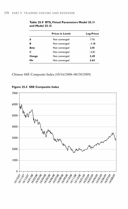
Chinese SSE Composite Index (10/16/2008–08/20/2009)
378 PART V TR ADING VOLUME A ND BEHAVIOR
Table 25.9 RTS, Fitted Parameters Model 25.11and Model 25.12
Prices in Levels Log-Prices
A Not converged 7.76
B Not converged –3.38
Beta Not converged 2.01
C Not converged –2.81
Omega Not converged 2.49
Phi Not converged 2.63
7000
6000
4000
3000
5000
2000
1000
0
16/10/07
16/11/07
16/12/07
16/01/08
16/02/08
16/03/08
16/04/08
16/05/08
16/06/08
16/07/08
16/08/08
16/09/08
16/10/08
16/11/08
16/12/08
16/01/09
16/02/09
16/03/09
16/04/09
16/05/09
16/06/09
16/07/09
16/08/09
Figure 25.5 SSE Composite Index

Comments on Anti-bubble Empirical ResultsThe previous analysis highlights some interesting results: the log-periodicmodel 25.11, which considers log-prices reached numerical convergence inalmost all cases, but at the same time the parameter β was almost alwaysgreater than 1, thus invalidating the underlying theoretical mechanism.Instead, the model which makes use of the prices in levels almost alwaysshowed values of β included between 0 and 1, and similarly 4 ω 15(except for the U.S. markets; see discussion below); therefore, our analysisseems to support the assumption that the speculative price decreases inrelation to a certain fundamental value p*; see Equations (25.3) and (25.4).Moreover, when the model using price in levels did not converge, such asfor the Chinese, Russian, and Brazilian markets, it is clear by looking at themarket plots that we are not in front of a possible anti-bubble structure; seeFigures 25.4 and 25.5.
Interestingly, the markets which most benefited from state intervention,like the U.S., Russian, and Chinese markets, are the ones for which the esti-mated coefficient β was greater than 1, or for which the log-periodic model(in price levels) did not converge. We remind that β is the parameter gov-erning the bubble growth and should be positive to ensure a finite price atthe critical time tc of the anti-bubble. In this regard, Zhou and Sornette(2005) highlighted that the cumulative effect of strong exogenous shocks,such as the U.S. Federal Reserve interest rate and monetary policies canprogressively detune the anti-bubble pattern; this seems exactly what hashappened with the U.S., Russian, and Chinese markets, where the massiveinjections of liquidity in the market has strongly modified the log-periodic
chapter 25 MODELING BUBBLES A ND A NTI-BUBBLES IN BEAR MARKETS 379
Table 25.10 Shanghai Composite, FittedParameters Model 25.11 and Model 25.12
Prices in Levels Log-Prices
A Not converged Not converged
B Not converged Not converged
Beta Not converged Not converged
C Not converged Not converged
Omega Not converged Not converged
Phi Not converged Not converged

structure. However, did these huge money injections finish to build up newmarket bubbles?
Bubbles in Bear Markets
Bastiaensen et al. (2009) were the first to analyze the bubble nature of themarket growth in the SSE Composite Index in July 2009, a month inadvance of the subsequent crash. They noted that “the Shanghai Compositeis the best performing large stock market in 2009 and is up 65 percent forthe year, and rising. To reach a targeted GDP growth of 8 percent, Chinesepolicy has turned to a bank model of massive lending, which has providedChina with sufficient liquidity to fuel this bubble.” Moreover, they pre-dicted that “the Shanghai Composite Index will reach a critical level aroundJuly 17–27, 2009.” The market peaked on August 4, 2009, and then lost 20percent in two weeks.
We repeat the previous analysis with a new computational methodologystill under development (as previously anticipated) but very promising, andwe consider also the case for the U.S. S&P 500 in August 2009, for theRussian RTS market in May 2009, and the S&P 500 in July 2007 for sakeof comparison, being that the peak of the market in the decade. The in-sample results for the model given by Equation (25.10), computed usingdata spanning from the global minima until one day before the marketpeak, are reported in Table 25.11.
Not surprisingly, all four markets show very similar estimated parame-ters, particularly with respect to the key coefficients β and ω. Besides, we
380 PART V TR ADING VOLUME A ND BEHAVIOR
Table 25.11 In-sample Fitted Parameters for Model 25.10
S&P 500 2007 S&P 500 2009 SSE 2009 RTS 2009
A 7.346 6.950 8.243 6.989
B –0.171 –0.498 –0.854 –1.804
Beta 0.801 0.778 0.552 0.818
C 0.037 –0.143 –0.031 0.207
Omega 5.140 4.102 5.702 6.371
Phi 3.035 2.180 3.952 5.931
tc 7.534 9.657 9.599 9.412
Estimation 06/13/2006– 03/09/2009 11/04/2008– 01/23/2009
Sample 07/12/2007– 08/28/2009 07/31/2009– 05/29/2009

want to propose here a graphical tool that we found extremely useful totrack the development of a bubble and to understand if a possible crash is insight, or at least a bubble deflation: we plot on the horizontal axis the date ofthe last observation in the estimation sample, and on the vertical axis the fore-casted crash date tc. If a change in the stock market regime is approaching,the (recursively) estimated tc should stabilize around a constant value closeto the turning point. We called such a plot the crash lock-in plot (CLIP).We report in Figure 25.6 the CLIPs for the previous four cases.
OUT-OF-SAMPLE EMPIRICAL ANALYSIS
We now examine the out-of-sample performances of the anti-bubble modelsand compare them with simple buy-and-hold and short-and-hold strategies.
chapter 25 MODELING BUBBLES A ND A NTI-BUBBLES IN BEAR MARKETS 381
Crash Lock-In Plot (CLIP):SP500 (July 2007)
Date of the last observation inthe estimation sample
7.55
7.5
7.5
7.45
7.45
Fore
cast
ed C
rash
Dat
e (T
C)
7.4
7.4
7.35
7.357.3
7.3
Crash Lock-In Plot (CLIP):SP500 (August 2009)
Date of the last observation inthe estimation sample
9.66
9.64
9.66
9.62
9.64Fo
reca
sted
Cra
sh D
ate
(TC
)
9.6
9.58 9.6 9.62
9.58
9.56
9.56
9.549.54
Crash Lock-In Plot (CLIP):SHANGAI (July 2009)
Date of the last observation inthe estimation sample
Fore
cast
ed C
rash
Dat
e (T
C)
Crash Lock-In Plot (CLIP):RTS (May 2009)
Date of the last observation inthe estimation sample
9.42
9.4
9.42
9.38
9.4
Fore
cast
ed C
rash
Dat
e (T
C)
9.36
9.32 9.34 9.389.36
9.34
9.3
9.32
9.39.28
9.6
9.55
9.6
9.45
9.5
9.45 9.5 9.55
9.4
9.4
9.35
9.39.35
Figure 25.6 Crash Lock-in Plots for the S&P 500, SSE Composite, andRussian RTS Indexes
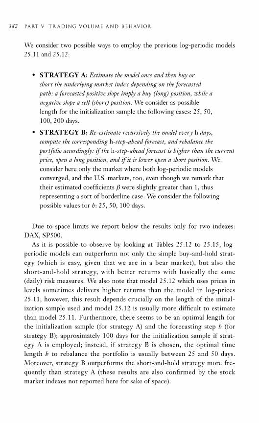
We consider two possible ways to employ the previous log-periodic models25.11 and 25.12:
• STRATEGY A: Estimate the model once and then buy or short the underlying market index depending on the forecasted path: a forecasted positive slope imply a buy (long) position, while anegative slope a sell (short) position. We consider as possible length for the initialization sample the following cases: 25, 50, 100, 200 days.
• STRATEGY B: Re-estimate recursively the model every h days,compute the corresponding h-step-ahead forecast, and rebalance theportfolio accordingly: if the h-step-ahead forecast is higher than the currentprice, open a long position, and if it is lower open a short position. Weconsider here only the market where both log-periodic modelsconverged, and the U.S. markets, too, even though we remark thattheir estimated coefficients β were slightly greater than 1, thusrepresenting a sort of borderline case. We consider the followingpossible values for h: 25, 50, 100 days.
Due to space limits we report below the results only for two indexes:DAX, SP500.
As it is possible to observe by looking at Tables 25.12 to 25.15, log-periodic models can outperform not only the simple buy-and-hold strat-egy (which is easy, given that we are in a bear market), but also theshort-and-hold strategy, with better returns with basically the same(daily) risk measures. We also note that model 25.12 which uses prices inlevels sometimes delivers higher returns than the model in log-prices25.11; however, this result depends crucially on the length of the initial-ization sample used and model 25.12 is usually more difficult to estimatethan model 25.11. Furthermore, there seems to be an optimal length forthe initialization sample (for strategy A) and the forecasting step h (forstrategy B); approximately 100 days for the initialization sample if strat-egy A is employed; instead, if strategy B is chosen, the optimal timelength h to rebalance the portfolio is usually between 25 and 50 days.Moreover, strategy B outperforms the short-and-hold strategy more fre-quently than strategy A (these results are also confirmed by the stockmarket indexes not reported here for sake of space).
382 PART V TR ADING VOLUME A ND BEHAVIOR

Table 25.12 Out-of-Sample Results for DAX Index, Model 25.11 with Log-Prices
Log-periodic model in Cumulative VaR VaR ES ESLOG-PRICES (2.11) Performance (%) Std.Dev (%) Skewness Kurtosis (99%) (99.9%) (99%) (99.9%)
STRATEGY A (25 days) 4.09% 0.72% 0.55 26.73 1.88% 4.27% 3.12% 4.64%
Buy-and-Hold 24.26% 2.24% 0.38 6.94 5.76% 10.69% 8.39% 10.74%
Short-and-Hold 24.26% 2.24% 0.38 6.94 6.06% 7.27% 6.75% 7.30%
STRATEGY A (50 days) 21.44% 2.25% 0.39 7.04 6.06% 7.27% 6.89% 7.30%
Buy-and-Hold 27.58% 2.25% 0.40 7.05 5.90% 10.69% 8.92% 10.74%
Short-and-Hold 27.58% 2.25% 0.40 7.05 6.06% 7.27% 6.89% 7.30%
STRATEGY A (100 days) 48.62% 2.35% 0.48 6.83 5.23% 10.69% 8.78% 10.74%
Buy-and-Hold 28.12% 2.35% 0.41 6.75 5.90% 10.69% 8.92% 10.74%
Short-and-Hold 28.12% 2.35% 0.41 6.75 6.06% 7.27% 6.89% 7.30%
STRATEGY A (200 days) 9.75% 2.67% 0.37 5.71 6.71% 7.27% 7.10% 7.30%
Buy-and-Hold 8.93% 2.67% 0.36 5.71 7.36% 10.69% 9.67% 10.74%
Short-and-Hold 8.93% 2.67% 0.36 5.71 6.71% 7.27% 7.10% 7.30%
STRATEGY B (25 days) 34.36% 2.25% 0.39 6.93 6.06% 7.27% 6.89% 7.30%
Buy-and-Hold 26.35% 2.25% 0.39 6.91 5.90% 10.69% 8.92% 10.74%
Short-and-Hold 26.35% 2.25% 0.39 6.91 6.06% 7.27% 6.89% 7.30%
STRATEGY B (50 days) 61.11% 2.30% 0.45 7.02 6.06% 7.27% 6.89% 7.30%
Buy-and-Hold 39.33% 2.31% 0.44 6.95 5.90% 10.69% 8.92% 10.74%
Short-and-Hold 39.33% 2.31% 0.44 6.95 6.06% 7.27% 6.89% 7.30%
STRATEGY B (100 days) 33.95% 2.42% 0.39 6.57 6.71% 7.27% 7.10% 7.30%
Buy-and-Hold 39.87% 2.42% 0.46 6.60 7.36% 10.69% 9.67% 10.74%
Short-and-Hold 39.87% 2.42% 0.46 6.60 6.71% 7.27% 7.10% 7.30%
383

Table 25.13 Out-of-Sample Results for DAX Index, Model 25.12 with Prices in Levels
Log-periodic model PRICES IN LEVELS Cumulative VaR VaR ES ES(2.12) Performance (%) Std.Dev (%) Skewness Kurtosis (99%) (99.9%) (99%) (99.9%)
STRATEGY A (25 days) 7.20% 0.27% 16.55 290.09 0.00% 0.00% 0.00% 0.00%
Buy-and-Hold 24.26% 2.24% 0.38 6.94 5.76% 10.69% 8.39% 10.74%
Short-and-Hold 24.26% 2.24% 0.38 6.94 6.06% 7.27% 6.75% 7.30%
STRATEGY A (50 days) 82.62% 2.24% 0.48 7.26 6.06% 7.27% 6.89% 7.30%
Buy-and-Hoid 27.58% 2.25% 0.40 7.05 5.90% 10.69% 8.92% 10.74%
Short-and-Hold 27.58% 2.25% 0.40 7.05 6.06% 7.27% 6.89% 7.30%
STRATEGY A (100 days) 24.29% 2.35% 0.37 6.87 5.15% 10.69% 8.34% 10.74%
Buy-and-Hold 28.12% 2.35% 0.41 6.75 5.90% 10.69% 8.92% 10.74%
Short-and-Hold 28.12% 2.35% 0.41 6.75 6.06% 7.27% 6.89% 7.30%
STRATEGY A (200 days) 9.75% 2.67% 0.37 5.71 6.71% 7.27% 7.10% 7.30%
Buy-and-Hold 8.93% 2.67% 0.36 5.71 7.36% 10.69% 9.67% 10.74%
Short-and-Hold 8.93% 2.67% 0.36 5.71 6.71% 7.27% 7.10% 7.30%
STRATEGY B (25 days) 53.70% 2.25% 0.38 6.98 6.06% 7.27% 6.89% 7.30%
Buy-and-Hold 26.35% 2.25% 0.39 6.91 5.90% 10.69% 8.92% 10.74%
Short-and-Hold 26.35% 2.25% 0.39 6.91 6.06% 7.27% 6.89% 7.30%
STRATEGY B (50 days) 22.24% 2.31% 0.39 6.89 6.06% 7.27% 6.89% 7.30%
Buy-and-Hold 39.33% 2.31% 0.44 6.95 5.90% 10.69% 8.92% 10.74%
Short-and-Hold 39.33% 2.31% 0.44 6.95 6.06% 7.27% 6.89% 7.30%
STRATEGY B (100 days) 1.48% 2.43% 0.34 6.48 6.71% 7.27% 7.10% 7.30%
Buy-and-Hold 39.87% 2.42% 0.46 6.60 7.36% 10.69% 9.67% 10.74%
Shiort-and-Hold 39.87% 2.42% 0.46 6.60 6.71% 7.27% 7.10% 7.30%
384

Table 25.14 Out-of-Sample Results for S&P500 Index, Model 25.11 with Log-Prices
Log-periodic model in Cumulative VaR VaR ES ESLOG-PRICES (2.11) Performance (%) Std.Dev (%) Skewness Kurtosis (99%) (99.9%) (99%) (99.9%)
STRATEGY A (25 days) 84.59% 2.32% 0.12 6.61 6.84% 9.35% 8.29% 9.41%
Buy-and-Hold 35.67% 2.32% 0.07 6.60 6.17% 10.25% 7.86% 10.60%
Short-and-Hold 35.67% 2.32% 0.07 6.60 6.31% 9.35% 8.20% 9.41%
STRATEGY A (50 days) 27.72% 2.36% 0.04 6.50 6.13% 10.25% 7.75% 10.60%
Buy-and-Hold 36.76% 2.36% 0.07 6.49 6.17% 10.25% 7.86% 10.60%
Short-and-Hold 36.76% 2.36% 0.07 6.49 6.31% 9.35% 8.20% 9.41%
STRATEGY A (100 days) 36.31% 2.47% 0.17 6.12 6.84% 9.47% 8.74% 9.86%
Buy-and-Hold 27.88% 2.47% 0.07 6.14 6.27% 10.25% 8.20% 10.60%
Short-and-Hold 27.88% 2.47% 0.07 6.14 6.95% 9.35% 8.58% 9.41%
STRATEGY A (200 days) 44.89% 2.78% 0.07 5.17 7.92% 9.35% 8.99% 9.41%
Buy-and-Hold 21.78% 2.78% 0.08 5.17 6.69% 10.25% 8.68% 10.60%
Short-and-Hold 21.78% 2.78% 0.08 5.17 7.92% 9.35% 8.99% 9.41%
STRATEGY B (25 days) 56.86% 2.36% 0.36 6.35 6.84% 10.25% 8.93% 10.60%
Buy-and-Hold 41.11% 2.37% 0.05 6.41 6.17% 10.25% 7.86% 10.60%
Short-and-Hold 41.11% 2.37% 0.05 6.41 6.31% 9.35% 8.20% 9.41%
STRATEGY B (50 days) 57.74% 2.41% 0.11 6.29 6.69% 10.25% 8.79% 10.60%
Buy-and-Hold 42.20% 2.41% 0.05 6.30 6.27% 10.25% 8.20% 10.60%
Short-and-Hold 42.20% 2.41% 0.05 6.30 6.95% 9.35% 8.58% 9.41%
STRATEGY B (100 days) 38.13% 2.67% 0.02 5.52 7.92% 9.35% 8.99% 9.41%
Buy-and-Hold 38.13% 2.67% 0.02 5.52 6.69% 10.25% 8.68% 10.60%
Short-and-Hold 38.13% 2.67% 0.02 5.52 7.92% 9.35% 8.99% 9.41%
385

Table 25.15 Out-of-Sample Results for S&P500 Index, Model 25.12 with Prices in Levels
Log-periodic modelPRICES IN LEVELS Cumulative VaR VaR ES ES(2.12) Performance (%) Std.Dev (%) Skewness Kurtosis (99%) (99.9%) (99%) (99.9%)
STRATEGY A (25 days) 21.54% 2.32% 0.23 6.58 5.41% 9.35% 7.40% 10.16%
Buy-and-Hold 35.67% 2.32% 0.07 6.60 6.17% 10.25% 7.86% 10.60%
Short-and-Hold 35.67% 2.32% 0.07 6.60 6.31% 9.35% 8.20% 9.41%
STRATEGY A (50 days) 13.03% 2.36% 0.25 6.51 6.27% 10.25% 8.37% 10.60%
Buy-and-Hold 36.76% 2.36% 0.07 6.49 6.17% 10.25% 7.86% 10.60%
Short-and-Hold 36.76% 2.36% 0.07 6.49 6.31% 9.35% 8.20% 9.41%
STRATEGY A (100 days 23.57% 2.47% 0.18 6.12 6.84% 9.47% 8.74% 9.86%
Buy-and-Hold 27.88% 2.47% 0.07 6.14 6.27% 10.25% 8.20% 10.60%
Short-and-Hold 27.88% 2.47% 0.07 6.14 6.95% 9.35% 8.58% 9.41%
STRATEGY A (200 days 46.14% 2.78% 0.07 5.18 7.92% 9.35% 8.99% 9.41%
Buy-and-Hold 21.78% 2.78% 0.08 5.17 6.69% 10.25% 8.68% 10.60%
Short-and-Hold 21.78% 2.78% 0.08 5.17 7.92% 9.35% 8.99% 9.41%
STRATEGY B (25 days) 54.68% 2.36% 0.37 6.35 6.84% 10.25% 8.93% 10.60%
Buy-and-Hold 41.11% 2.37% 0.05 6.41 6.17% 10.25% 7.86% 10.60%
Short-and-Hold 41.11% 2.37% 0.05 6.41 6.31% 9.35% 8.20% 9.41%
STRATEGY B (50 days) 57.74% 2.41% 0.11 6.29 6.69% 10.25% 8.79% 10.60%
Buy-and-Hold 42.20% 2.41% 0.05 6.30 6.27% 10.25% 8.20% 10.60%
Short-and-Hold 42.20% 2.41% 0.05 6.30 6.95% 9.35% 8.58% 9.41%
STRATEGY B (100 days) 38.13% 2.67% 0.02 5.52 7.92% 9.35% 8.99% 9.41%
Buy-and-Hold 38.13% 2.67% 0.02 5.52 6.69% 10.25% 8.68% 10.60%
Short-and-Hold 38.13% 2.67% 0.02 5.52 7.92% 9.35% 8.99% 9.41%
386

CONCLUSION
We reviewed the theory of log-periodic models for bubble and anti-bubblemodeling and we performed an empirical analysis with different world stockmarket indexes to verify whether a medium-term trading strategy based onthese models can outperform simple buy-and-hold or short-and-hold strate-gies. We found that these models can outperform both the buy-and-holdstrategy (easy) and the short-and-hold strategy, but this result depends cru-cially on the initialization sample and/or the frequency for portfolio rebal-ancing, where the latter is usually between 25 and 50 days.
REFERENCES
Bastiaensen, K., Cauwels, P., Sornette, D., Woodard, R., and Zhou, W.-X.(2009) The Chinese Equity Bubble: Ready to Burst. Working paper,ETH Zurich, Switzerland. Available at: http://arxiv.org/abs/0907.1827
Blanchard, O.J. (1979) Speculative Bubbles, Crashes and Rational Expecta-tions. Economics Letters, 3(4): 387–389.
Chang, G. and Feigenbaum, J. (2006) A Bayesian Analysis of Log-PeriodicPrecursors to Financial Crashes. Quantitative Finance, 6(1):15–36.
Johansen, A., and Sornette, D. (1999) Financial Anti-Bubbles: Log-periodicityin Gold and Nikkei Collapses. International Journal of Modern Physics C,10(4): 563–575.
Johansen, A., Ledoit, O., and Sornette, D. (2000) Crashes as CriticalPoints. International Journal of Theoretical and Applied Finance, 3(2):219–255.
Lin, L., Ren, R.E., and Sornette, D. (2010) A Consistent Model of ExplosiveFinancial Bubbles With Mean-Reversing Residuals. Quantitative Finance,forthcoming.
Sornette, D. (2003) Why Stock Markets Crash (Critical Events in ComplexFinancial Systems). Princeton, NJ: Princeton University Press.
Sornette, D. and Johansen, A. (1997) Large Financial Crashes. Physica A,245(3–4): 411–422.
Sornette, D., Johansen, A., and Bouchaud, J.P. (1996) Stock Market Crashes,Precursors and Replicas. Journal de Physique I, 6(1): 167–175.
Sornette, D. and Woodard, R. (2009) Financial Bubbles, Real Estate Bubbles,and the Financial and Economic Crisis. Proceedings of APFA7 (Applicationsof Physics in Financial Analysis), forthcoming.
chapter 25 MODELING BUBBLES A ND A NTI-BUBBLES IN BEAR MARKETS 387

Xin, Z. and Wheatley, A. (2009) China’s CIC Wealth Fund Muscles Up asMarkets Recover. Beijing (Reuters). Available at: http://www.reuters.com/article/ousiv/idUSTRE57S0D420090829
Zhou, W.X., and Sornette, D. (2005) Testing the Stability of the 2000–2003US Stock Market Antibubble. Physica A, 348(2): 428–452.
388 PART V TR ADING VOLUME A ND BEHAVIOR

389
26C H A P T E R
Strategic FinancialIntermediaries withBrokerage Activities
Laurent Germain, Fabrice Rousseau, and Anne Vanhems
ABSTRACT
In this chapter, we study the strategic use by banks of their brokerageactivities. We consider a situation where N competing banks are engagedin brokerage activities and have access to private information about the liq-uidation value of a risky asset. Selling brokerage activities, banks collectorders from their clients and can use their brokerage divisions to enhancetheir own profits. This order flow is considered in our model as uninfor-mative, i.e., as being noise. The banks’ ability to observe part of the totalorder flow, i.e., its own volume and the one of its clients, even though itdoes not incorporate any private information, gives valuable informationconcerning the level of noise trading in the market. We show that takingadvantage of that information, i.e., the strategic use of their brokerageactivities, increases the banks’ expected profits. However, we prove thatthe aggregate expected profit is lower when banks strategically use theirbrokerage activities.

INTRODUCTION
Investment banks and financial institutions invest in the collection and theproduction of information; in particular, they possess their own researchdivisions. One of the uses of this information is proprietary trading wherebybanks trade for their own account. Nevertheless, financial institutions may have other sources of information. They can infer private informationfrom their clients. Indeed, some banks may know that some of their clientshave private information and infer that private information from theirclients’ trading. Moreover, as financial institutions can also act as brokersand transmit noninformative orders on behalf of their customers, they arealso able to infer part of the total order flow observed by market makers.This duality in the role of banks that on the one hand act as traders and onthe other hand act as brokers can induce a conflict of interest between theclients and the financial institutions as the banks could use their clients’information strategically.
Empirical evidence in Michaely and Womack (1999) shows a particularconflict of interest faced by investment banks. On the one hand, they haveincentives to transmit reliable information to their customers to maintaintheir reputation. On the other hand, they can use this information forserving their own interests and distort it. Some financial scandals in theUnited States have highlighted this type of conflict of interest for the useof the information by banks. Indeed, the banks’ financial analysts whogather information can release false information to the market to serve thebanks’ or their clients’ financial interests.
This raises the following issues. What are the consequences of suchleakages in the Chinese walls of financial institutions? Should brokerageactivities be banned for financial institutions which develop their owntrading divisions?
We develop a model where financial institutions produce information,trade for their own account, and observe their clients’ orders in the frameof their brokerage activities. We assume that the banks’ customers do notpossess private information and are, therefore, considered to be noise trad-ers. Small customers using the banks to transmit their orders to the marketare not reputed to be informed. The customer’s order flow is then purenoise and does not contain any private information. Given these brokerageactivities, banks have access to some valuable information concerning part
390 PART V TR ADING VOLUME A ND BEHAVIOR

of the liquidity trading in the market stemming from their customers.When engaging in proprietary trading, banks can use this knowledge totheir benefit.
This chapter is close to the models of Fishman and Longstaff (1992),Roell (1990), and Sarkar (1995) who study dual trading for brokeragefirms. The main difference between these models and our work is that, inthe present model the f inancial institutions also trade for their ownaccount. In Fishman and Longstaff (1992), the brokers bear a fixed cost ofmaintaining a brokerage business and a variable cost for filling an order.Under such a framework, the authors derive the competitive commissionfor filling orders. Nevertheless, Fishman and Longstaff (1992) do notmodel the competition between broker houses in the market. In ourmodel, banks compete in the financial market when trading and face thesame cost structure.
Biais and Germain (2002) and Germain (2005) study the conflict ofinterest between financial institutions that trade for their own account andat the same time set up a fund for their clients. They derive the optimalcontracts that solve this conflict of interest. In particular, Germain (2005)shows that at the equilibrium the banks can commit to add an optimal levelof noise to diminish their competition. In our model, we do not study whatwould be the optimal contract but derive the optimal trading strategy forfinancial intermediaries. Brennan and Chordia (1993) analyze the casewhere banks undertake brokerage activities. They study the optimal brokerage schedule for the case where the broker sells information to thecustomers. We do not address the question of selling information but focuson the critical issue of free riding on information derived by the order flowtransmitted by the customers.
Rochet and Vila (1994) study the case of a monopolistic trader whoobserves the noise trading. In our chapter, we consider the case of N banks.However, we restrict our analysis to a linear/normal model which is not thecase in the Rochet and Vila (1994) paper. We assume that the banks are strate-gic, informed, and have heterogeneous beliefs, for such a framework we derivethe following results. At the equilibrium, the financial institutions that observesome noise trading behave optimally by trading in the opposite direction oftheir customers’ orders. Moreover, we find that the liquidity and the banks’responsiveness to private information are reduced. We show that the expectedprofit of a bank that observes part of the noise trading is always greater than
chapter 26 STR ATEGIC FINA NCIAL INTERMEDIAR IES 391

the profit she would get otherwise. In addition, we also show that if part of theliquidity order flow is observed the aggregate expected profit is reduced.
The chapter is organized as follows. In the next section, we study the casewhere informed traders do not observe any noise from their customers. In the third section of this chapter, we analyze the general case where somenoise can be observed. In the last section we conclude. All proofs are gathered in the chapter’s Appendix.
THE BENCHMARK MODEL: NO NOISE ISOBSERVED
This model is identical to Didri and Germain (2009), hereafter DG (2009).Consider a financial market with a risky asset whose final value V
~is
normally distributed with zero mean and variance σ2v. There are three
types of agents:
• N risk neutral informed traders who observe a signal Si concerningthe future value of the asset before trading, such that
• Liquidity traders who submit market orders U, where U → N(0,σ 2U).
• Risk neutral market makers, who observe the aggregate volume Wand set rationally the price in a Bayesian way.
Assume that V~
,ε1,…,εN, U are mutually independent.A strategy for the informed agent i is a function Xi corresponding to his
market order and depending on the observed signal Si. These strategies
determine the aggregate order flow Let P denote the
equilibrium price determined by the market makers and πi (V P)Xi theresulting trading profit of insider i. The market makers behave competi-tively, upon observing the aggregate order flow W, their expected profit isequal to zero, i.e., E(V P|W) 0. Each informed agent i chooses Xi tomaximize her expected profit E(πi |Si). Moreover, the equilibrium is said tobe linear if there exists λ, such that P λW.
We now derive the unique perfect Bayesian linear equilibrium of this game.
W X Uii
N
= +=
∑1
.
392 PART V TR ADING VOLUME A ND BEHAVIOR
∀ = = + ∀ = →i N S V i ,...,N Ni i i i1 1 0,..., , , ,ε ε σwhere 22( ) .

Proposition 1: There exists a unique linear equilibrium defined by
Proof: See Appendix.
Proposition 2: Expected Profits
• At the equilibrium, the expected profit of agent i is given by
• At the equilibrium, the expected aggregate profit is given by
Proof: See Appendix.This case is considered as the benchmark case and will be compared to
the subsequent results. This situation is equivalent to the one where nobanks or financial institutions undertake brokerage activities and as a resultdo not have access to any of the liquidity order flow.
chapter 26 STR ATEGIC FINA NCIAL INTERMEDIAR IES 393
∀ = =
=
⎧⎨⎪
⎩⎪
i N X S
P Wwhere witi i i1,..., ; **
**
β
λ, ( hh j
j
v
τσ
σ=
2
2)
∀ = =
+
+( )
+
+( )
i N i
U vi
i
i
i
1
1
1 2
1
1 2
2
,..., , **π
σ στ
τ
τ
τ22
1
12
1
1 11 2i
N
ii
N
= =
∑ ∑⎛
⎝
⎜⎜
⎞
⎠
⎟⎟
++
⎡
⎣⎢
⎤
⎦⎥
τ
π π
σ στ
τ** *= =
+
+( )
⎛
⎝
⎜⎜
⎞
⎠
⎟⎟
=
=
∑∑
ii
NU v
i
ii
N
1
21
1
1
1 2
22
1
1 11 2
++
⎡
⎣⎢
⎤
⎦⎥
=
∑τ ii
N
βσ
σ τ
τ
τi
U
v i
j
jj
N** =
+( )+
+( )
⎛
⎝
⎜⎜
⎞
⎠
⎟⎟
=
−
∑11 2
1
1 22
1
112
21
1 1
1 2and
λ
σ
σ
τ
τ**
=+
+( )
⎛
⎝
⎜⎜
⎞
⎠
⎟⎟
=
−
∑U
v
j
jj
N
112
1
1 11 2
++
⎡
⎣⎢⎢
⎤
⎦⎥⎥=
∑τ jj
N

In the next section, we analyze the case where some of the noise tradingis observed by financial institutions.
THE GENERAL MODEL: WHEN SOME NOISE IS OBSERVED
Our objective is to study how a better knowledge of the noise trader orderflow will affect the profit of the agents.
In order to distinguish between observed and unobserved liquiditytrading, we decompose the global order U into two parts U U0 Uun,where U0 represents the observed liquidit y trading (decomposed in subparts corresponding to the N informed traders) and Uun the unobservedpart. The observed part Uo Σ
N
i1 Uo
i is itself decomposed into N subpartscorresponding to the N informed traders: each informed trader i canobserve the liquidity order Uo
i. This decomposition of the total variance ofthe liquidity trading will prove useful when studying the impact of ob-serving some of this liquidity trading by informed traders.
We assume that: U0 → N(0, θσ 2U), Uun → N(0,(1 θ)σ 2
U) with 0 θ 1,and, i1,…, N, Uo
i → N(0αiσ2U), with i1,…, N, 0 αi 1 and Σ
N
i1 α i 1.
The parameters θ and α1,…, αN capture the impact of observing noisetrading. This can be understood as follows. Assume that the liquiditytraders who want to trade Uo
i , do not submit this order directly to themarket but instead direct bank i to do it on their behalf. As this banktrades for her own account, she might use this piece of information (sizeof her clients order) when deciding the quantity to trade. The parameterαi can be understood as the fraction of the overall observed noise tradingobserved by agent i, in other words, this corresponds to the particularbanks’ brokerage activity. When, αi 0, this implies that Uo
i 0 in thatcase agent i does not observe any of the noise trading order flow. Theparameter θ corresponds to the overall brokerage activity in the market.
To summarize, we can consider the following different situations:
• θ 0: No noise is observed (no brokerage activity). This setting isidentical to DG (2009).
• θ 0: Part of the noise is observed. If, θ 1, there is no unobservedliquidity order flow. In that case all the customers’ orders arechanneled to the market by the banks. When i 1, … , N,αi 0,all informed traders observe part of the liquidity trading. If for onebank i we have that αi 0, then at least one financial institution does
394 PART V TR ADING VOLUME A ND BEHAVIOR

not observe any liquidity order. On the contrary, if for bank i αi 1and θ 1, then that bank observes all the liquidity order flow.
Assume that V~
, ε1,…,εN, U01,…,U0
N, Uun are mutually independent.A strategy for the informed agent i is a function Xi corresponding to his
market order and depending on Si and on the amount of liquidity tradingobserved if any is observed. Given the informed market orders and the liquidityorder flow, the aggregate order flow is equal to W Σ
N
i1 Xi U. Let P denote
the equilibrium price determined by the market makers and πi (V P)Xi theresulting trading profit of insider i. As before, due to competition in marketmaking, the price must be such that E(V P|W) 0. Each informed agent ichooses Xi to maximize her expected profit E(πi |Si, U0
1). We now derive theunique perfect Bayesian linear equilibrium of this game.
Proposition 3: There exists a unique equilibrium defined by
Proof: See Appendix.Proposition 4: Expected Profits
• At the equilibrium, the expected profit of agent i is given by: i 1,…,N,
chapter 26 STR ATEGIC FINA NCIAL INTERMEDIAR IES 395
∀ ≥ = −
= +⎛
⎝⎜⎜
⎞
⎠⎟⎟
=
∑
i X S U
P X U
i i i io
jj
N
1 12
1
, ,*
*
β
λ
where (∀ = =i N ii
v
12
2, ..., , )τ
σ
σ
βσ θ
σ τ
τ
τi
U
v i
i
ii
N* =
−
+( )+
+( )
⎛
⎝
⎜⎜
⎞
⎠=
∑1
1 21
1 2
34
21
⎟⎟⎟
=− +
+( )
⎛−
=
∑
12 3
42
1
1 1 1
1 2and
λ
σ θ
σ
τ
τ*
U
v
i
ii
N
⎝⎝
⎜⎜
⎞
⎠
⎟⎟
++
⎡
⎣⎢
⎤
⎦⎥
−
=
∑
12
1
1 11 2τ ii
N
.
π α θ
σ στ
τθ
τ
τ
i i
U vi
i
i
i
* ( , ) =
+
+( )−
+
+( )
1
1 21
1
1 2
234
2ii
N
ii
N
i U v
= =
∑ ∑⎛
⎝
⎜⎜
⎞
⎠
⎟⎟
++
⎡
⎣⎢
⎤
⎦⎥
+
1
12
1
1 11 2τ
α θσ σ
44 1
1
1 2
1 11 2
34
21
12
−
+
+( )
⎛
⎝
⎜⎜
⎞
⎠
⎟⎟
++
=
∑
θ
τ
τ
τ
i
ii
N
ii==∑
⎡
⎣⎢
⎤
⎦⎥
1
N

• At the equilibrium, the expected aggregate profit is given by
Proof: See Appendix.
Interpretation of the Equilibrium
The strategy of bank i depends explicitly on the part of the order flow Uo
i that she observes. Half of the observed order flow is revealed by hermarket order. This reduces the “amount” of noise in the aggregate orderf low. As a result market makers price more aggressively leading to adecrease in market’s liquidity. It is then optimal for the banks to scale downthe size of their market order to reduce their impact on the price. Banks arethen revealing less of their private information. Moreover, one can see thatthe bank i’s responsiveness to private information does not depend on theparticular fraction of the order flow observed by bank i, αi. It only dependson the overall fraction of the order flow observed, θ. The more of the orderflow is channeled to the market by banks, the more banks scale down theirtrading.
Interpretation of the Individual Profit
• The individual expected profit for bank i is the sum of two terms: thefirst one corresponds to the individual expected profit with no noisemultiplied by and the second one depends explicitly on αi. The former term takes into account the effect of the observation of a fraction θ of the entire liquidity order flow, i.e., on the overallbrokerage activity in the market. It affects all the banks whether theyundertake brokerage activities or not. The latter term embodies theimpact for bank i of her own brokerage activity which gives her theobservation of part of the noise trading α iθ.
• The first term decreases with θ. As the fraction of the observed noisetrading increases, banks decrease their trading intensity and liquidity
1 34− θ
396 PART V TR ADING VOLUME A ND BEHAVIOR
π θ π α θ
σ στ
τ* *( ) ( , )= =
+
+( )
⎛
=
=
∑∑
i ii
NU v
i
ii
N
1
21
1
1 2⎝⎝
⎜⎜
⎞
⎠
⎟⎟
++
⎡
⎣⎢
⎤
⎦⎥
−
−
=
∑
12
1
341 1
1 2
22 1
τ
θ
θ
ii
N

decreases. This leads to a decrease in the individual expected profit of the banks. This term captures the negative effect of brokerageactivities in the market. The second term increases with both θ andαi. In other words, the more bank i observes of the liquidity orderflow the larger her expected profit.
• The bank undertaking brokerage activities earns an expected profitlarger than that of a bank that cannot observe any noise. The morenoise is observed by bank i, through an increase of αi, the less theother banks earn in expectation.
Interpretation of the Aggregate Profit
• When θ 0, we find the results obtained in DG (2009).
• The impact of brokerage on aggregate profit is given by the
multiplicative term , which is always less or equal to 1.
In particular, we have A(0) A(1) 1 . The aggregate expectedprofit when no noise is observed is the same as when all the noise isobserved. Moreover, when some noise is observed, the aggregateexpected profit diminishes. However, it decreases for 0 θ 2/3 andincreases for 2/3 θ 1.
Particular Case: All the Noise Trading Is Observed (θ 1)
In the case where θ 1, all the customers’ order flow is directed to the mar-ket by the financial institutions.
• The aggregate profit is the same as when no noise is observed.
• The expected profit of trader i is equal to i 1,…, N,
A( )θθ
θ=
−
−
22 1 3
4
chapter 26 STR ATEGIC FINA NCIAL INTERMEDIAR IES 397
π α θ
σ στ
τ
τ
τ
i i
U vi
i
i
ii
* ( , ) =
+
+( )
+
+( )=
14
1
1 2
1
1 2
2
21
NN
ii
N
i U v
∑ ∑⎛
⎝
⎜⎜
⎞
⎠
⎟⎟ +
+
⎡
⎣
⎢⎢
⎤
⎦
⎥⎥
+
=
12
1
1 11 2
2
1
τ
α σ σ
++
+( )
⎛
⎝
⎜⎜
⎞
⎠
⎟⎟
++
⎡
⎣
⎢
=
=
∑
∑
τ
τ
τ
i
ii
N
ii
N
1 2
1 11 2
21
12
1⎢⎢
⎤
⎦
⎥⎥

• The banks reveal half of the liquidity trading observed. If wecompare that with Proposition 1, we find that banks reduce theirtrading intensity by half. The market liquidity is also reduced by half.
• The individual expected profit is increasing with the proportion of thenoise observed by the particular bank. However, if the entire noise isobserved, the aggregate expected profit is not affected and is equal tothe one in the DG (2009) model.
CONCLUSION
In this model we analyze the case where financial institutions sell brokerageactivities and trade for their own account. We show that the banks optimally incorporate half of the noise trading observed, due to their brokerage activities, and decrease their information responsiveness as well.When analyzing both the banks’ individual expected profit and the aggre-gate expected profit, the following results are obtained. For each financialinstitution the expected profit is increasing with the noise observed or heramount of brokerage activities. This implies that if a bank does not engagein brokerage activities her expected profit is smaller than if she does. Theaggregate profit when some of the order flow is channeled to the market bybanks is always lower than the aggregate profit in DG (2009), where nonoise is observed. However, for the extreme case where all the noise tradingorder flow is directed to the market by banks, the aggregate expected profitis equal to the one in DG (2009). In a different paper, we generalize thisapproach to the case where the banks trade for their account, sell brokerageactivities, and sell information to their clients.
REFERENCES
Brennan, M.J. and Chordia, T. (1993) Brokerage Commission Schedules.The Journal of Finance, 48(4): 1379–1402.
Biais, B. and Germain, L. (2002) Incentive Compatible Contracts for theSale of Information. The Review of Financial Studies, 15(4): 987–1003.
Dridi, R. and Germain, L. (2009) Noise and Competition in StrategicOligopoly. Journal of Financial Intermediation, 18(2): 311–327.
Fishman, M.J. and Longstaff, F.A. (1992) Dual Trading In Futures Market.The Journal of Finance, 47(2): 643–671.
Germain, L. (2005) Strategic Noise in Competitive Markets for the Sale ofInformation. Journal of Financial Intermediation, 14(2): 179–209.
398 PART V TR ADING VOLUME A ND BEHAVIOR

Michaely, R. and Womack, K.L. (1999) Conf lict of Interest and theCredibility of Underwriter Analyst Recommendations. The Review ofFinancial Studies, 12(4): 653–686.
Rochet, J-C. and Vila, J-L. (1994) Insider Trading without Normality.Review of Economic Studies, 61(1): 131–152.
Roell, A. (1990) Dual Capacity Trading and the Quality of the Market.Journal of Financial Intermediation, 1(2): 105–124.
Sarkar, A. (1995) Dual Trading: Winners, Losers and Market Impact.Journal of Financial Intermediation, 4(1): 77–93.
APPENDIX
Proof of Proposition 1: Proposition 1 is a particular case of Proposition3 with θ 0, i 1,…, N αi 0 and then U0 0.
Proof of Proposition 2: Follow the steps of Proposition 4 with θ 0 and i1,…, N αi 0.
Proof of Proposition 3: Agent i maximizes her conditional expectedprofit:
Using that are mutually independent, we denote,
for i 1,… N,
V U U UNo
No un, , ..., , , ..., ,ε ε1 1
chapter 26 STR ATEGIC FINA NCIAL INTERMEDIAR IES 399
q x E x V x X U U Ui j io
jo un
j ij i
( ) = − + + + +⎛
⎝
⎜⎜
⎞
⎠
⎟
≠≠
∑∑ λ⎟⎟
⎡
⎣
⎢⎢
⎤
⎦
⎥⎥
⎛
⎝
⎜⎜⎜
⎞
⎠
⎟⎟⎟
= ( ) −
S U
xE V S U x
i io
i io
,
, λ 2 −−⎛
⎝
⎜⎜
⎞
⎠
⎟⎟ − ( )
≠
∑λ λxE X S U xE U S Ujj i
i io
io
i io, ,
max ,x R j
j ii iE x V x X U S U
∈≠
− + +⎛
⎝
⎜⎜
⎞
⎠
⎟⎟
⎡
⎣
⎢⎢
⎤
⎦
⎥⎥∑ λ oo i N
⎛
⎝
⎜⎜⎜
⎞
⎠
⎟⎟⎟
=, , ...,1
q x xE V S x x E X S U xUi i j i io
j iio( ) = ( ) − − ( ) −
≠
∑ λ λ λ2 , .

Moreover, using the assumption that j 1,…N, Xj is a function of Sj
and U0i and is independent of U0
i for all i j, we obtain
400 PART V TR ADING VOLUME A ND BEHAVIOR
XS
U E X S i Nii
iio
j ij i
=+
− − ( ) =
⇔
≠
∑12 1
12
12
1λ τ
, ,...,
,, with
X X U i N
XS
i i io
ii
i
= + =
=+
12
1
12 1
, ,...,
λ τ−− ( ) =
≠
∑12
1E X S i Nj ij i
, ,...,
λ * cov( , )var( )
cov( , )
var(= =
+
+
=
∑
V WW
V X U
X
ii
N
i
1
UU
V S U U
i
N
i i io
i
N
)
cov( , )
va
*
=
=
∑
∑=
−⎛
⎝⎜
⎞
⎠⎟+
1
1
12
β
rr( )*βi i io
i
N
S U U−⎛
⎝⎜
⎞
⎠⎟+
=
∑ 121
βτ λ τi
i jj
Na a**
,=+
= ++
⎡
⎣⎢⎢
⎤
⎦⎥⎥=
∑1 21 1 1
1 21
and
λβ σ
β σ β σ
*
*
* *
=⎛
⎝⎜
⎞
⎠⎟ + ( ) +
=
=
∑
∑
i vi
N
ii
N
v i i
2
1
1
2
2 2 2 (( )1 14
2 2
1
− +=
∑ θ σ θσu ui
N
q x xE V S x x E X S U xUi i j i io
j iio( ) = ( ) − − ( ) −
=
≠
∑ λ λ λ2 ,
xxS
xU x x E X Si
iio
j ij i1
2
+− − − ( )
≠
∑τ
λ λ λ ,
The necessary and sufficient first order conditions arewith τσ
σii
v
=2
2.
We can then derive the same proof as in DG (2009) and prove that thereexists a unique linear solution X
~ *i β*
iSi,i 1,…, N. Using the normalityassumption and the mutual independence of V
~,ε1, …, εN, U 0
N, Uun, we canwrite β*
i and λ* as follows:
with a being independent of i. Both the normality of each component andthe mutual independence assumption allow us to identify the parameter λ*.

We then identify and both parameters and
β*i,i 1,…, N. This ends the proof of Proposition 3.
Proof of Proposition 4: We have, for all i 1,…, N.
expressions , we obtain:
. Replacing the parameter
a by its expression allows us to derive the final result. The aggregate profit
is simply obtained by computing . This ends the proof
of Proposition 4.
π θ π α θ* *( ) ( , )==
∑ i ii
N
1
π α θσ τ
τ
α θσi i
v i
i
i ua
a* ( , ) =
+( )+( )
+⎡
⎣
⎢⎢
⎤
⎦
2
2
21
1 2 4⎥⎥⎥
++
⎛
⎝⎜⎜
⎞
⎠⎟⎟
=
−
∑1 11 21
1
τ jj
N
βτ λ τi
i jj
Na a**
=+
= ++
⎡
⎣⎢⎢
⎤
⎦⎥⎥=
∑1 21 1 1
1 21
and
1λ *
au
vi
ii
N=
−
+
+
⎛
⎝⎜⎜
⎞
⎠⎟⎟
=
∑
1 34
11 2 2
1
2
θ σ
στ
τ
.
( )
chapter 26 STR ATEGIC FINA NCIAL INTERMEDIAR IES 401
11 3
4
1
2
1
1
λβ
β τ
β
θ
**
*
*
= +( )
+
−⎛
⎝⎜
=
=
=
∑∑
∑i
i
N i ii
N
ii
N
⎞⎞
⎠⎟
=+
++
=
=
∑
∑σ
β στ
τ
τu
ii
N
vi
i
ii
N
a a
2
1
2
211
1 21 2
*
( )11
1 2
1 34
11 21
1
2
2
+
+
−⎛
⎝⎜
⎞
⎠⎟
+=
= ∑∑
τ
θ σ
στii
Ni
N u
vii
a==
∑1
N
π α θ βi i i i i ioE X V P E S U* *( , ) .= −( )⎡
⎣⎤⎦ = −
⎛
⎝⎜
⎞
⎠⎟ 1
2V S U Ui i
i
No un− + +
⎧⎨⎪
⎩⎪
⎫⎬⎪
⎭⎪
⎛
⎝⎜⎜
⎞
⎠⎟⎟
=
∑λ β* *
1
12
⎡⎡
⎣⎢⎢
⎤
⎦⎥⎥
= −
.
( , )* * * *Using the π α θ β σ λ β σi i i v i v2 2 ββ λ β σ τ
λα θσj
j
N
i v i i u* * *
*
=
∑ − ( ) +1
2 2 2
4

This page intentionally left blank

403
27C H A P T E R
Financial Markets,Investment Analysis, andTrading in Primaryand SecondaryMarkets
André F. Gygax
ABSTRACT
Over the past four decades trading volumes in most financial markets havesteadily increased. This paper investigates the motivations for tradingusing fundamental analysis, arbitrage and technical analysis. It is arguedthat the large trading volumes in primary markets could be a consequenceof the automation of the trading process, the growth of electronic tradingand the emergence of hig-frequency trading strategies. Similarly, increasedlevels of investor sophistication and the involvement of financial specialistswith technical backgrounds have led to many financial innovations in sec-ondary or derivatives markets. Although trading volumes in option mar-kets and many futures markets are high, U.S. single stock futures (SSFs)volumes are low when compared to the trading volume in the underlyingequity securities and corresponding options contracts. This is surprising asSSFs can be utilized as a cost effective technique to hedge and rebalanceportfolio positions.
INTRODUCTION
Most financial markets have undergone a rapid evolution over the past fourdecades. Many of the changes have coincided with seminal developments infinancial economics, such as the pricing of options, the pricing of debt, and arbitrage pricing (Black and Scholes, 1973; Merton, 1974; Ross, 1976).This extent of the evolution of financial markets, however, would not havebeen possible without significant advances in the underlying technology ofcomputing and the advancement of the Internet and electronic communica-tion networks (ECNs). The deeper understanding of the pricing of securi-ties along with the automation of the trading process have changed the roleand nature of traditional exchanges (Di Noia, 2001; Chemmanur and Fulghieri, 2006), allowed new players to enter financial markets (Stoll,2008), and have generally led to an increase in trading volumes, reductionin bid ask spreads and the speed at which buy or sell orders are executed.These developments raise a few questions: What types of financial analysismotivate contemporary trading? How can the large volumes of trading beexplained? Where does trading take place? Each of these questions will bediscussed in the following sections.
INVESTMENT ANALYSIS AND TYPES OF TRADING
Using a broad classification, investment analysis can be performed in twoways: through fundamental or technical analysis. The goal of this section isto investigate how various forms of investment analysis motivate or result inthe trading of securities rather than to engage in the debate whether tech-nical analysis is a sound financial approach compared with classical analysissuch as fundamental analysis or the identification of arbitrage opportunities(Treynor and Ferguson, 1985; Brock, Lakonishok, and LeBaron, 1992; Sullivan, Timmermann, and White, 1999).
Trading Motivated by Fundamental Analysis
Fundamental analysis is an approach motivated by classical finance princi-ples of valuation. Here an analyst decides whether a security is over- orundervalued relative to its fundamental value. If, for example, a security isundervalued, an agent would buy the security and hold it until it has
404 PART V TR ADING VOLUME A ND BEHAVIOR

reached its fair valuation level. This is commonly referred to as a buy-and-hold trading strategy.
Arbitrage Motivated Trading
A second motivation for trading is that an agent has identified an arbitrageopportunity in the market. This could be the case when a trader knows thatthe price of a security differs from its fundamental value (Dow and Gorton,1994). The agent then decides whether to try to take advantage of the per-ceived mispricing or to wait and benefit from a potential gain due to addi-tional possible divergence in prices (Kondor, 2009). Most arbitrageopportunities do not persist in the market and that is the reason for whyelectronic trading using sophisticated algorithms is a widely used techniqueto exploit short-term mispricing in the market.
Technical Analysis and Technical Trading
In the academic literature technical analysis has received little attention rela-tive to fundamental analysis (Lo, Mamaysky, and Wang, 2000). In contrast,the practitioner literature provides many illustrations of how technical trad-ing is used in trading by investment institutions. Technical analysis is mostlybased on historical information and does not deal with the estimation or calculation of expected prices based on a theoretical asset pricing model. Ithas been most successfully used in currency markets (Osler, 2003).
The goal of technical analysis is to identify patterns in historical priceand/or volume data (Blume, Easley, and O’Hara, 1994). These patternscould be used to implement a trading strategy using technical rules (Taylor,1994). This could be achieved by employing genetic algorithms (Allen andKarjalainen, 1999; Lo, Mamaysky, and Wang, 2000; Wang, 2000). Somesimple and popular technical trading rules are the moving average and trad-ing break rules such as “head-and-shoulders” or “double-bottoms” (Brock,Lakonishok, and LeBaron, 1992; Kho, 1996; Zhu and Zhou, 2009). Techni-cal analysis could also be employed by an agent to identify to what extentnew information has been priced into a security (Treynor and Ferguson,1985; Brown and Jennings, 1989; Grundy and McNichols, 1989). Brunner-meier (2005) shows that informed traders can benefit from technical analy-sis if they know both past prices and some private information. Such aprivate information signal could be imprecise or noisy. Technical analysis
chapter 27 TR ADING in Primary and Secondary Markets 405

could also motivate a trader to pursue a momentum or contrarian tradingstrategy (Keim and Madhavan, 1995; Okunev and White, 2003).
Other Motivations for Trading
Trading can also be motivated by noninformation-based reasons. Forexample, fund managers adjust portfolio holdings when cash contributionsor withdrawals take place (Keim and Madhavan, 1995). Such situationscould arise due to workplace changes or retirement of fund unit holders.Cash inflows or outflows could also be related to good “relative” or poor“absolute” fund performance (Ikovic and Weisbenner, 2009). Furthermore,index funds have to trade shares when the constituents of an index change.Finally, trading could also be induced for tax or seasonality reasons(Poterba and Weisbenner, 2001; Ikovic, Poterba, and Weisbenner, 2005).
COMPOSITION OF TRADING VOLUME AND TRADING
How can the large increases in trading volumes in primary equity, bond,or currency markets be explained? Three major trends in the developmentof financial markets serve as possible explanations: (1) the growth of elec-tronic trading; (2) the emergence of high-frequency trading; and (3) thelevel of investor sophistication. These trends have all contributed to thedramatic increase in trading volumes. Below, these trends are discussed inmore detail.
Over the past 20 years electronic trading has gradually substituted floortrading of securities. Simultaneously, the level of investor sophistication hasincreased and financial markets have witnessed the hiring of people withnontraditional and nonfinancial backgrounds such as engineers, physicists,mathematicians, and computer scientists. These professionals have not onlybeen able to employ complex financial formulae but also to develop power-ful electronic platforms through which they operate sophisticated and oftenautomated trading algorithms. This combination of skill sets has con-tributed to the rapid growth of electronic trading.
By 2008, electronic trading accounted for 40 percent of daily tradingvolume according to Deutsche Börse (Grant and Gangahar, 2008). In theU.S. equities markets, according to the Tabb Group, the emergence of
406 PART V TR ADING VOLUME A ND BEHAVIOR

electronic trading has also led to a substantial increase in high-frequencytrading through the use of flash orders amounting to about 73 percent ofdaily trading volume (Mackenzie, 2009). Flash orders are high-frequencyorders which are executed within a fraction of a second by using auto-mated trading platforms and algorithms. This practice is most common onthe NASDAQ OMX market and BATS, an ECN, but not encouraged bythe NYSE Euronext exchange.
The popularity of electronic and high-frequency trading has helpedBATS to become the third largest U.S. equity market behind NYSEEuronext and NASDAQ. A possible reason for this rapid climb of BATScould be that ECNs have helped to improve quote quality (Huang, 2002).Other reasons that have helped ECNs to attract trading, and in particularinformed trading, are greater anonymity and the speed of order execution(Barclay, Hendershott, and McCormick, 2003). In addition, electronic trad-ing has facilitated the emergence of alternative trading systems such as dayand after-hours crossing systems (Conrad, Johnson, and Wahal, 2003).
TRADING IN PRIMARY VERSUS SECONDARY MARKETS
Trading is not confined to the primary markets but also takes place in thesecondary or derivatives markets. To implement a trading strategy a tradermight establish long or short positions in the derivatives market rather thanin the underlying security. This approach has the advantage of being lesscapital intensive. Options can also play an important role during takeoverattempts. In addition, a trader can combine call and put options to execute avolatility trading strategy. However, the statistics in Lakonishok et al.(2007) show that the combination of call and put options, such as straddlesand strangles, represent only a small percentage of trading. In contrast, Panand Poteshman (2006) show that informed trading represents a significantfraction of option trading and that this can create some predictability aboutfuture stock prices. Table 27.1 provides stock and index option volume andopen interest information for the first three quarters of 2008 for all U.S.listed option contracts. The volume data demonstrate a stark difference intrading volumes between stock options and index options. Apart fromMarch 2008 stock call option volumes are always higher than put stockoption volumes. The opposite is true for index options. In each month
chapter 27 TR ADING in Primary and Secondary Markets 407
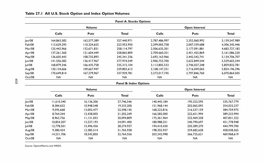
Table 27.1 All U.S. Stock Option and Index Option Volumes
Panel A. Stocks Options
Volume Open Interest
Calls Puts Total Calls Puts Total
Jan/08 164,863,582 162,577,389 327,440,971 2,787,486,997 2,352,060,992 5,139,547,989Feb/08 113,629,295 110,324,655 223,953,950 2,299,005,758 2,007,339,688 4,306,345,446Mar/08 125,442,966 132,671,831 258,114,797 2,506,635,301 2,177,091,881 4,683,727,182Apr/08 137,261,360 121,604,449 258,865,809 2,709,660,351 2,451,425,869 5,161,086,220May/08 136,605,443 108,735,893 245,341,336 2,692,163,966 2,442,542,741 5,134,706,707Jun/08 141,556,582 136,417,967 277,974,549 2,906,753,700 2,622,849,544 5,529,603,244Jul/08 168,879,346 166,435,758 335,315,104 3,113,805,533 2,746,027,248 5,859,832,781Aug/08 130,134,666 109,667,947 239,802,613 3,108,147,331 2,716,049,065 5,824,196,396Sep/08 170,649,814 167,279,967 337,929,781 3,273,017,745 2,797,846,760 6,070,864,505Oct/08 NA NA NA NA NA NA
Panel B: Index Options
Volume Open Interest
Calls Puts Total Calls Puts Total
Jan/08 11,610,340 16,136,206 27,746,546 140,445,184 195,322,595 335,767,779Feb/08 8,384,652 10,948,548 19,333,200 151,968,144 202,065,093 354,033,237Mar/08 9,595,668 13,002,477 22,598,145 168,222,816 216,537,159 384,759,975Apr/08 8,764,244 12,438,005 21,202,249 166,582,000 222,651,994 389,233,994May/08 8,963,756 11,131,053 20,094,809 175,361,964 232,469,358 407,831,322Jun/08 10,854,207 13,237,193 24,091,400 180,988,251 240,790,697 421,778,948Jul/08 12,778,501 15,496,436 28,274,937 194,410,430 250,389,270 444,799,700Aug/08 9,380,424 12,385,514 21,765,938 198,355,937 259,682,628 458,038,565Sep/08 14,221,706 18,542,850 32,764,556 203,242,998 266,725,621 469,968,619Oct/08 NA NA NA NA NA NA
Source: OptionMetrics and WRDS.
408

more put index options are traded than index call options. A possible expla-nation for this finding could be that traders and investors were more con-cerned about overvaluation at the market level but at the same time werenot too concerned about valuation levels at the individual stock levels.
In other financial markets, particularly the bond, currency, and com-modities markets, futures contracts are more frequently traded thanoptions. A major benefit of the futures market is that both long and shortpositions can be established easily and cost-effectively. In addition, theproblem of short-sales constraints in the primary market does not arise inthe futures market (Nagel, 2005). Despite this, in the United States shortselling in the equities market by far outweighs trading volumes in shortpositions in the secondary SSF market (Shastri, Thirumalai, and Zutter,2008). The high volumes are illustrated in Diether, Lee, and Werner (2009)who show that short selling represents approximately a quarter of all NYSEand 31 percent of NASDAQ transactions.
In contrast, the relatively low volumes in the SSF market are shown inTables 27.2 and 27.3. Columns 2 and 3 in Table 27.2 show that in the UnitedStates trading volumes in SSFs have declined markedly in August 2008. Thisis one month prior to the dramatic fall in equities markets in September andOctober 2008. Column 5 in Table 27.2 shows the corresponding tradingvolumes for the NYSE Liffe Universal Stock Futures (USF) market. Thedata show a low volume for August but a high volume for September 2009.Table 27.3 presents OneChicago SSF trading volumes over the period –5 to5 trading days relative to the Lehman Brothers bankruptcy announcementon September 15, 2008. Although trading volumes fell during and aroundthe announcement, they increased within a few days.
A possible explanation for the low level of trading in SSF contracts couldbe that these contracts were previously banned in the United States due tothe Shad-Johnson Accord and only reintroduced on November 8, 2002 bythe OneChicago and NQLX (a joint venture of NASDAQ and Liffe)(Shastri, Thirumalai, and Zutter, 2008). The comparison in Table 27.2 ofOneChicago with other markets that trade SSFs shows that only the London- (UK) based NYSE Liffe market has significantly higher volumesand open interest than OneChicago. SSF volumes on the Hong KongExchange (HKEX) have remained low and the Sydney Futures Exchange(SFE), a division of the Australian Stock Exchange (ASX), has delisted SSFcontracts in March 2008 apparently due to low volumes and the emergenceof contracts for difference (CFDs).
chapter 27 TR ADING in Primary and Secondary Markets 409

410
Table 27.2 Single Stock Futures Volume Statistics for the U.S., UK, Hong Kong, and Australia
OneChicago NYSE LIFFE HKEX SFE (ASX)
Number of Average Annual / Open Annual / Open Annual / Annual /Futures on Daily Monthly Interest Monthly Interest Monthly Open Monthly
Single Stocks Volume SSF Volume SSF SSF Volume USF USF Volume SF Interest SF Volume SF
(1) (2) (3) (4) (5) (6) (7) (8) (9)
2000 NA NA NA NA 3,664,560 75,207 3,322 21 8,817
2001 NA NA NA NA 6,193,283 429,139 6,945 455 12,545
2002 79 NA NA NA 7,570,175 193,944 21,006 405 29,286
2003 NA 15,556 NA 153,866 7,004,235 444,996 18,654 1,020 47,822
2004 NA NA 1,922,726 154,621 13,115,815 181,473 17,274 1,821 29,986
2005 NA 21,937 5,528,046 1,600,000 11,365,103 411,125 13,069 1,750 38,156
2006 482 32,000 7,923,499 1,351,320 18,147,980 1,130,568 102,010 4,260 10,843
2007 491 NA 8,105,963 370,420 45,249,036 4,713,663 351,514 5,954 11,242
Jan/08 491 28,157 591,297 581,712 1,483,291 4,376,255 NA NA NA
Feb/08 527 11,551 219,476 NA 3,510,457 4,768,434 NA NA NA
Mar/08 601 13,354 267,076 365,441 5,607,523 5,038,164 NA NA DEL
Apr/08 694 14,646 322,205 492,882 6,796,541 8,167,882 NA NA DEL
May/08 800 12,382 260,024 294,896 8,690,132 5,922,453 NA NA DEL
Jun/08 800 26,840 563,641 423,867 11,428,282 5,465,938 NA NA DEL

411
Jul/08 800 17,852 392,744 314,158 3,371,143 6,439,136 NA NA DEL
Aug/08 800 7,924 166,399 270,516 2,812,466 5,100,107 19,209 7,592 DEL
Sep/08 989 8,800 184,792 199,566 12,477,190 4,734,828 41,891 8,269 DEL
Oct/08 1,148 7,164 164,778 127,600 7,457,505 7,416,847 36,300 8,122 DEL
Nov/08 1,142 7,192 136,647 91,511 6,441,116 4,762,983 31,987 9,973 DEL
Dec/08 1,120 6,142 135,122 68,290 9,378,708 4,707,192 23,396 9,449 DEL
2008 1,120 3,404,201 68,290 79,454,354 4,707,192 257,015 9,449 100
Jan/09 1,131 6,721 134,411 98,962 9,680,449 7,605,483 23,750 6,350 DEL
Feb/09 1,137 6,032 114,604 85,918 5,121,659 5,382,386 16,619 6,310 DEL
Mar/09 1,134 6,628 145,808 70,606 9,647,551 5,551,249 31,168 9,208 DEL
Apr/09 1,132 3,632 76,279 72,734 14,160,668 10,663,839 22,228 12,136 DEL
May/09 1,141 4,684 93,676 87,607 16,049,208 8,138,571 15,888 4,600 DEL
Jun/09 1,150 NA NA NA 14,750,555 5,179,549 31,433 14,806 DEL
Jul/09 1,166 NA NA NA 13,438,543 7,747,484 26,081 10,477 DEL
Source: SIRCA, OneChicago, NYSE LIFFE, Hong Kong Exchange, ASX Sydney.

CONCLUSION
The volume of trading in financial markets has experienced tremendousgrowth during the past four decades. This growth was possible due to changesin the regulatory environment but was mostly driven by the rapid expansion ofelectronic trading platforms and the sophisticated use of technical algorithmswhich have greatly increased the speed of order execution. So far, equity andcurrency markets have experienced the greatest technological changes. Otherfinancial markets, such as bonds, real estate, derivatives, and over-the-countermarkets are developing in response to regulatory calls for increased trans-parency. Finally, increasingly sophisticated investors require even more effi-cient and effective platforms for trade execution.
REFERENCES
Allen, F. and Karjalainen, R. (1999) Using Genetic Algorithms to FindTechnical Trading Rules. Journal of Financial Economics, 51(2): 245–271.
Barclay, M.J., Hendershott, T., and McCormick, D.T. (2003) CompetitionAmong Trading Venues: Information and Trading on Electronic Com-munications Networks. Journal of Finance, 58(6): 2637–2665.
Black, F. and Scholes, M. (1973) Pricing of Options and Corporate Liabilities.Journal of Political Economy, 81(3): 637–654.
412 PART V TR ADING VOLUME A ND BEHAVIOR
Table 27.3 U.S. SSF Volumes around Lehman Brothers Bankruptcy
Number of Exchange for Block Open Date Contracts Total Volume Physical Volume Volume Interest
09/08/2008 3,165 7,569 26 1,590 280,925
09/09/2008 3,165 9,322 1,544 125 281,784
09/10/2008 3,165 13,624 8 8,820 282,067
09/11/2008 3,173 5,138 1,406 0 282,543
09/12/2008 3,173 6,497 37 3,500 286,989
09/15/2008 3,169 5,400 1,437 244 286,271
09/16/2008 3,169 6,014 827 0 286,991
09/17/2008 3,173 7,707 168 0 287,641
09/18/2008 3,173 14,838 720 296 294,540
09/19/2008 3,173 18,507 1,688 0 300,266
09/22/2008 3,131 10,563 2,105 2,500 175,000
Source: SIRCA and OneChicago.

Blume, L., Easley, D., and O’Hara, M. (1994) Market Statistics and TechnicalAnalysis—The Role of Volume. Journal of Finance, 49(1), 153–181.
Brock, W., Lakonishok, J., and LeBaron, B. (1992) Simple Technical TradingRules and the Stochastic Properties of Stock Returns. Journal of Finance,47(5): 1731–1764.
Brown, D.P. and Jennings, R.H. (1989) On Technical Analysis. Review ofFinancial Studies, 2(4): 527–552.
Brunnermeier, M.K. (2005) Information Leakage and Market Efficiency.Review of Financial Studies, 18(2): 417–457.
Chemmanur, T. J. and Fulghieri, P. (2006) Competition and Cooperationamong Exchanges: A Theory of Cross-Listings and Endogenous List-ing Standards. Journal of Financial Economics, 82(2): 455–489.
Conrad, J., Johnson, K.M., and Wahal, S. (2003) Institutional Trading andAlternative Trading Systems. Journal of Financial Economics, 70(1):99–134.
Di Noia, C. (2001) Competition and Integration among Stock Exchanges inEurope: Network Effects, Implicit Mergers and Remote Access. EuropeanFinancial Management, 7(1): 39–72.
Diether, K.B., Lee K.H., and Werner, I.M. (2009) Short-Sale Strategies andReturn Predictability. The Review of Financial Studies, 22(2): 575–607.
Dow, J. and Gorton, G. (1994) Arbitrage Chains. Journal of Finance, 49(3):819–849.
Grant, J. and Gangahar, A. (2008) Spotlight on Role of E-trading in Volatility.Financial Times, October 29. Available at: http://www.ft.com/cms/s/0/c9814b98-a5e7–11dd–9d26–000077b07658.html?nclick_check1
Grundy, B.D. and McNichols, M. (1989) Trade and Revelation of Informationthrough Prices and Direct Disclosure. Review of Financial Studies, 2(4):495–526.
Huang, R.D. (2002) The Quality of ECN and Nasdaq Market MakerQuotes. Journal of Finance, 57(3): 1285–1319.
Ikovic, Z., Poterba, J., and Weisbenner, S. (2005) Tax-Motivated Trading byIndividual Investors. American Economic Review, 95(5): 1605–1630.
Ikovic, Z. and Weisbenner, S. (2009) Individual Investor Mutual FundFlows. Journal of Financial Economics, 92(2): 223–237.
Keim, D.B. and Madhavan, A. (1995) Anatomy of the Trading Process—Empirical Evidence on the Behavior of Institutional Traders. Journal ofFinancial Economics, 37(3): 371–398.
chapter 27 TR ADING in Primary and Secondary Markets 413

Kho, B.C. (1996) Time-Varying Risk Premia, Volatility, and Technical Trad-ing Rule Profits: Evidence from Foreign Currency Futures Markets.Journal of Financial Economics, 41(2): 249–290.
Kondor, P. (2009) Risk in Dynamic Arbitrage: The Price Effects of Con-vergence Trading. Journal of Finance, 64(2): 631–665.
Lakonishok, J., Lee, I., Pearson, N.D., and Poteshman, A.M. (2007) OptionMarket Activity. Review of Financial Studies, 20(3): 813–857.
Lo, A.W., Mamaysky, H., and Wang, J. (2000) Foundations of TechnicalAnalysis: Computational Algorithms, Statistical Inference, and EmpiricalImplementation. Journal of Finance, 55(4): 1705–1765.
Mackenzie, M. (2009) High-frequency Trading Under Scrutiny. FinancialTimes, July 28. Available at: http://www.ft.com/cms/s/0/d5fa0660–7b95–11de–9772–00144feabdc0.html?nclick_check1
Merton, R.C. (1974) The Pricing of Corporate Debt—Risk Structure ofInterest Rates. Journal of Finance, 29(2): 449–470.
Nagel, S. (2005) Short Sales, Institutional Investors and the Cross-Sectionof Stock Returns. Journal of Financial Economics, 78(2): 277–309.
Okunev, J. and White, D. (2003) Do Momentum-Based Strategies stillWork in Foreign Currency Markets? Journal of Financial and Quantita-tive Analysis, 38(2): 425–447.
Osler, C.L. (2003) Currency Orders and Exchange Rate Dynamics: AnExplanation for the Predictive Success of Technical Analysis. Journal ofFinance, 58(5): 1791–1819.
Pan, J. and Poteshman, A.M. (2006) The Information in Option Volumefor Future Stock Prices. Review of Financial Studies, 19(3): 871–908.
Poterba, J.M. and Weisbenner, S.C. (2001) Capital Gains Tax Rules, Tax-Loss Trading, and Turn-of-the-Year Returns. Journal of Finance, 56(1):353–368.
Ross, S.A. (1976) Arbitrage Theory of Capital Asset Pricing. Journal ofEconomic Theory, 13(3): 341–360.
Shastri, K., Thirmalai, R.S., and Zutter, C.J. (2008) Information Revelationin the Futures Market. Journal of Futures Market, 28(4): 335–353.
Stoll, H.R. (2008) Future of Securities Markets: Competition or Consoli-dation. Financial Analysts Journal, 64(6): 15–26.
Sullivan R., Timmermann, A., and White, H. (1999) Data-Snooping, Tech-nical Trading Rule Performance, and the Bootstrap. Journal of Finance,54(4): 1647–1691.
414 PART V TR ADING VOLUME A ND BEHAVIOR

Taylor, S.J. (1994) Trading Futures Using a Channel Rule—A Study of thePredictive Power of Technical Analysis with Currency Examples. Jour-nal of Futures Markets, 14(2): 215–235.
Treynor, J.L. and Ferguson, R. (1985) In Defense of Technical Analysis.Journal of Finance, 40(3): 757–773.
Wang, J. (2000) Trading and Hedging in S&P 500 Spot and Futures Mar-kets Using Genetic Programming. Journal of Futures Markets, 20(10):911–942.
Zhu, Y.Z. and Zhou, G.F. (2009) Technical Analysis: An Asset AllocationPerspective on the Use of Moving Averages. Journal of Financial Eco-nomics, 92(3): 519–544.
chapter 27 TR ADING in Primary and Secondary Markets 415

This page intentionally left blank
417
28C H A P T E R
Trading andOverconfidence
Ryan Garvey and Fei Wu
ABSTRACT
Using proprietary data from a U.S. broker-dealer, we test Gervais andOdean’s (2001) learning model of overconfidence in professional stock trad-ers. We find that traders place more bets following prior trading gains.Traders who are most influenced by their prior trading profits experiencelower performance, but not the lowest. While we find a strong link betweenprior performance and subsequent trading activity, our results indicate thatthe relationship weakens with time. Traders who are active for longer(shorter) periods of time are less (more) likely to be overconfident.
INTRODUCTION
Theoretical models predict that traders in financial markets are overconfi-dent, i.e., they have a tendency to overestimate the precision of theirbeliefs or forecasts, and they tend to overestimate their abilities.1 Overcon-fidence is an important issue for traders because traders who are overconfi-dent will lower their performance by entering into suboptimal bets and/orengaging in too many bets. While financial models predict that, on aver-age, traders in financial markets are overconfident, there is little empiricalresearch directly testing the theoretical predictions of overconfidencemodels on individual traders.2 In our chapter, we test whether or not theactions of U.S. stock traders are consistent with the learning model ofoverconfidence developed by Gervais and Odean (2001), hereafter GO

(2001). In GO (2001), overconfidence is determined endogeneously andfluctuates over time as traders learn from their prior experiences. Early on,when traders are less experienced, they are more likely to overweight thepossibility that their success is due to superior ability. This learning bias(i.e., self-attribution bias) can cause traders to be overconfident. As tradersgain more experience over time, though, they gain a better understandingof their abilities, and trader’s level of overconfidence subsequently declines.
Using unique data on U.S. stock traders, we find empirical evidence sup-porting three key predictions of the GO (2001) overconfidence model.
1. Traders learn from their prior successes and become overconfident.
2. Overconfident traders experience lower performance, though notnecessarily the lowest.
3. Experience matters. Traders become less overconfident over time.
The remainder of our study is organized as follows. First, we describethe sample data. Next, we provide empirical testing of overconfidence the-ory. Our empirical testing is focused around the GO (2001) learning modelof overconfidence. Lastly, we provide concluding remarks.
DATA
The purpose of our study is to empirically examine how traders learn abouttheir ability and how (if ) a bias in this learning can create overconfidenttraders. Such an analysis requires data on traders who are active over anextended period of time. To satisfy this requirement, we collect sample datafrom a U.S. broker-dealer who provides their clients with direct marketaccess (DMA). Brokers providing DMA services tend to attract moresophisticated traders because they allow their users to control where andhow their orders are routed for execution. Consequently, they also tend toattract clients who trade often and in large sizes. A considerable amount ofdaily trading activity in U.S. equity markets flows through DMA brokeragefirms. For example, Goldberg and Lupercio (2004) find that approximately40 percent of NASDAQ and NYSE trading volume is executed by activetraders (25 trades per day) who use U.S. brokers offering DMA services.
We collect data over the sample period October 7, 1999 to August 1,2003. The firm mainly attracted clients who had an interest in tradingNASDAQ-listed stocks. This is because NASDAQ stocks trade in multiple
418 PART V TR ADING VOLUME A ND BEHAVIOR

trading venues and the primary benefit of using a DMA broker is the abilityto route orders to various trading venues. In contrast, NYSE-listed tradingis mainly confined to a single trading location during our sample period.3
Because clients opened an account at our firm with the primary intent ofbenefiting their NASDAQ trading, and because a high percentage of trad-ing activity occurs on NASDAQ stocks, our analysis focuses on tradersNASDAQ-listed stock trading. The data are in the form of a transactiondatabase and provide information such as the identity of the trader, thetime of submission, the time of execution, the market where the order wassent, the execution size, the execution price(s), the stock symbol, the ordertype, the contra party, and various other information concerning the tradeexecution (or cancellation) and executing account.
In order to examine traders who are active over an extended period oftime, we first restrict our analysis to traders who are active during morethan 250 trading days (approximately one trading year) over the sampleperiod (969 trading days). We then select accounts that have an intradayroundtrip match rate exceeding 90 percent. A high intraday match rate isdesirable because it enables us to calculate a robust measure of performanceand ensures that we are examining traders who receive frequent feedbackon their performance. Because we lack opening position data, we cannotaccurately measure performance for traders who engage in longer termtrading strategies. Performance is based on matching up the intradaytrades, using a first-in, first-out matching algorithm. For each stock andtrader, we match opening trades with the subsequent closing trade(s) in thesame day. In order to do this, we search forward in time each day until theopening position is closed out, keeping track of accumulated intradayinventory and the corresponding prices paid or received.
Table 28.1 provides some summary statistics on the sample data. Overall,the analysis is based on 109 traders, who combined to execute more than 6billion shares (3.6 million trades) over the near four-year sample period.The dollar value traded exceeds $60 billion and the traders managed togenerate over $4 million in trading profits during a bearish market. Oursample period was considered a very “challenging” market trading environ-ment. For example, the revenues of NASDAQ broker-dealers with a market-making operation fell over 70 percent during 2000 to 2004 (GAO,2005). The GAO cited the sharp decline in stock prices, heightened compe-tition, the switch to a smaller tick size, etc., for the sharp decline in tradingrevenues during our sample period.
chapter 28 TR ADING A ND OVERCONFIDENCE 419

Table 28.1 provides summary statistics for 109 traders, who tradedthrough a U.S. broker-dealer, over the approximate four-year period endingAugust 2003. Each trader is active for more than 250 sample trading days.
EMPIRICAL RESULTS
Our empirical results are organized around three key predictions from theGO (2001) learning model of overconfidence. The three hypotheses we testare as follows.
Hypothesis 1: Past Success Leads to Subsequent Increases inTrader Activity (i.e., Overconfidence)
GO (2001) suggest that trader activity is the primary testable implication ofoverconfidence theory and that traders increase their activity when theyhave experienced prior gains. We empirically test this prediction by esti-mating a trader fixed-effects regression.4
Log(Sharesi,t) αi β1Cum.Prof.i.t 1 Σ Contols εi,t (28.1)
Using trader-specific constant terms, αi is desirable to control for varia-tions across traders. The regression dependent variable Log (Sharesi,t) is thelog number of daily shares traded and the main independent variable ofinterest, Cum. Proof.
i, t 1 is trader cumulative performance (divided by$10,000) from the first day availabe up to t 1. Because factors other thanpast performance might (also) cause traders to increase (decrease) theiractivity, we include several regression control variables that have beenshown in prior financial studies to serve as motives for trading. The control
420 PART V TR ADING VOLUME A ND BEHAVIOR
Table 28.1 Summary Statistics
Aggregate Daily Average
Dollar Value Traded $60,732,249,829 $557,176,604
Shares Traded 6,084,739,456 55,823,298
Number of Trades 3,673,442 33,701
Profits $4,145,121 $38,029

variables are the log-daily trading volume on NASDAQ, the daily volatilityof NASDAQ, which is measured by the difference in the NASDAQ com-posite index daily high/low divided by the opening level, the daily (lagged)return on the NASDAQ composite index, and a dummy variable that takesthe value of 1, or 0 otherwise, if trading occurs at the end of the calendaryear (i.e., December).
Regression results are reported in Table 28.2. The cumulative perfor-mance coefficient is positive (0.0113) and highly significant (t stat 10.15),indicating that increases in trader prior performance lead to subsequentincreases in trader activity. This result is consistent with H1. The controlvariables reveal the influence of other factors on trader activity. When dailyvolume and price returns are higher, trader activity is also higher. Tradersincrease their activity at the end of the year (i.e., December), too. Whenprice volatility is higher, traders decrease their activity.
The fixed-effects regression dependent variable is trader activity (log-daily number of shares traded). The independent variable include tradercumulative profit up to time t 1 (1/$10,000), the log-daily trading vol-ume on NASDAQ, the daily volatility of NASDAQ, which is measured bythe difference in the NASDAQ composite index daily high/low divided bythe opening level, the daily (lagged) return on the NASDAQ compositeindex, and a dummy variable that takes the value of 1, or 0 otherwise, iftrading occurs in the month of December.
chapter 28 TR ADING A ND OVERCONFIDENCE 421
Table 28.2 Prior Performance and Subsequent TradingActivity
Coefficient t Statistic
Cumulative Profit (1/$10,000) >0.0113** 10.15
Daily NASDAQ Volume (Log) 0.2999** 12.65
Daily NASDAQ Volatility 5.5038** 11.86
Daily NASDAQ Return 1.4075** 6.58
NASDAQ Return (t 1) 0.0626 0.28
NASDAQ Return (t 2, t 20) 0.4174** 7.51
December Dummy 0.0690** 3.64
Trader Fixed Effects Yes
Adjusted R2 0.0124
**,*Indicates significance at the 1% and 5% level, respectively.

Hypothesis 2: Overconfident Traders Experience LowerPerformance, Though Not Necessarily the Lowest
To test this hypothesis, we first conduct individual trader ordinary leastsquares regressions using the same regression variables described above (H1 testing). For example, trader activity is used as the dependent variableand cumulative performance is used as the main independent variable. Theregressions also use the volume, return, volatility, and year-end controls.After estimating regressions for each of the 109 traders, we then grouptraders into quintiles based on the magnitude of their cumulative perfor-mance coefficient. Traders in Q1 have the highest cumulative performancecoefficient (or they are the most overconfident) and traders in Q5 have thelowest cumulative performance coefficient. Lastly, we compute the meantotal/daily profit (performance) for each group. The results are reported inTable 28.3.
Traders with high overconfidence regression coefficients are, on average,profitable in a bearish market, yet they underperform Q3 traders, who canbe considered neutral traders. The performance differences are quite large.For example, the average daily profit of Q3 traders is more than 18 timeshigher than Q1 traders and nearly 3 times higher than Q2 traders. Themost overconfident traders underperform the average across all traders,though they do not have the worst performance. For example, Q5 traderswho are negatively influenced by their past success perform much worsethan Q1 traders.
Individual ordinary least squares regressions are conducted for eachtrader (109) by regressing log-daily number of shares traded on cumulativeprofit and controls (see Table 28.2 regression variables). Traders are thensorted into quintiles based on the magnitude of their cumulative profit
422 PART V TR ADING VOLUME A ND BEHAVIOR
Table 28.3 Overconfidence and Performance
Mean CumulativeProfit Coefficient Mean Total Profit Mean Daily Profit
Q1 Largest 0.2679 $8,627 $16
Q2 0.0133 $48,382 $101
Q3 0.0022 $139,593 $294
Q4 0.0347 $3,277 $22
Q5 Smallest 0.2477 $5,119 $13

coefficient. The mean cumulative profit coefficient, total profit and dailyprofit are reported for each quintile.
Hypothesis 3: Traders Learn from Trading andOverconfidence Declines Over Time
Gervais and Odean (2001) predict that as traders gain more trading experi-ence, they will also gain a better understanding of their abilities and over-confidence will subsequently diminish over time. This can be empiricallytested by including a time effect in our prior regression used to test H1.We add two more variables to our fixed-effects regression.
Log(Sharesi,t) αi β1 Cum. Prof.i,t1 β2 Timet β2
Timet Cum. Prof.i,t1 Σ Contols εi,t (28.2)
The first added variable,Timet, measures elapsed calendar time in monthsstarting at the beginning of our sample period (Time 1 for the firstmonth of our sample period, Time 2 for the second month, etc.). Time isincluded in order to separate general effects associated with the passage oftime from time varying (or declining) overconfidence. The second addedvariable Timet Cum. Prof.i, t 1 is an interaction term. This is used toaccount for the possibility that traders learning bias will dissipate with timeas their experience grows or that cumulative profit will have a declininginfluence on subsequent trader decisions. As predicted by H3, we expect anegatively significant cumulative profit*time coefficient.
The regression results are reported in Model 1 of Panel A, Table 28.4.Consistent with H3, the cumulative profit*time coefficient is negative(0.0479) and highly significant (t stat 8.03), which suggests that tradersoverconfidence tendency decreases over time through learning by trading.In Table 28.4, Panel B, we report the estimated deviations of trader activity(shares traded) with respect to trader cumulative profits, evaluated for each period of Time (1 through 46). The deviations steadily decrease andremain statistically significant up to Time 27. This implies that, on average,traders’ learning bias (or overconfidence tendency) runs its course by about27 months.
The fixed-effects regression dependent variable is trader activity (log-daily number of shares traded). Independent variables include: time, which
chapter 28 TR ADING A ND OVERCONFIDENCE 423
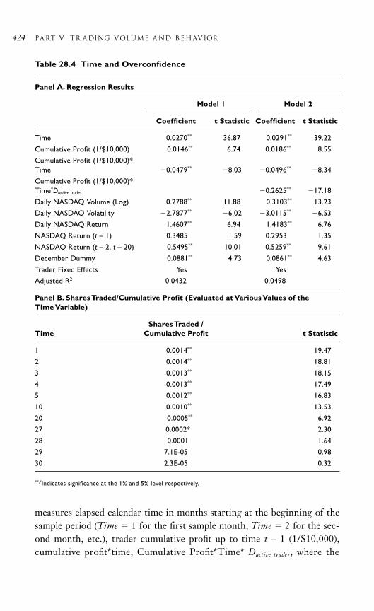
424 PART V TR ADING VOLUME A ND BEHAVIOR
Table 28.4 Time and Overconfidence
Panel A. Regression Results
Model 1 Model 2
Coefficient t Statistic Coefficient t Statistic
Time 0.0270** 36.87 0.0291** 39.22
Cumulative Profit (1/$10,000) 0.0146** 6.74 0.0186** 8.55
Cumulative Profit (1/$10,000)*Time 0.0479** 8.03 0.0496** 8.34
Cumulative Profit (1/$10,000)*Time*Dactive trader 0.2625** 17.18
Daily NASDAQ Volume (Log) 0.2788** 11.88 0.3103** 13.23
Daily NASDAQ Volatility 2.7877** 6.02 3.0115** 6.53
Daily NASDAQ Return 1.4607** 6.94 1.4183** 6.76
NASDAQ Return (t – 1) 0.3485 1.59 0.2953 1.35
NASDAQ Return (t – 2, t – 20) 0.5495** 10.01 0.5259** 9.61
December Dummy 0.0881** 4.73 0.0861** 4.63
Trader Fixed Effects Yes Yes
Adjusted R2 0.0432 0.0498
Panel B. Shares Traded/Cumulative Profit (Evaluated at Various Values of the Time Variable)
Shares Traded / Time Cumulative Profit t Statistic
1 0.0014** 19.47
2 0.0014** 18.81
3 0.0013** 18.15
4 0.0013** 17.49
5 0.0012** 16.83
10 0.0010** 13.53
20 0.0005** 6.92
27 0.0002* 2.30
28 0.0001 1.64
29 7.1E-05 0.98
30 2.3E-05 0.32
**,*Indicates significance at the 1% and 5% level respectively.
measures elapsed calendar time in months starting at the beginning of thesample period (Time 1 for the first sample month, Time 2 for the sec-ond month, etc.), trader cumulative profit up to time t – 1 (1/$10,000),cumulative profit*time, Cumulative Profit*Time* Dactive trader, where the

dummy variable Dactive trader takes the value of 1, or 0 otherwise, if an obser-vation is associated with an active trader (top 30 percent based on totalnumber of trades), the log-daily trading volume on NASDAQ, the dailyvolatility of NASDAQ, which is measured by the difference in the NAS-DAQ composite index daily high/low divided by the opening level, thedaily (lagged) return on the NASDAQ composite index, and a dummyvariable that takes the value of 1, or 0 otherwise, if trading occurs in themonth of December. Panel B. (Model 1) shows the estimated deviations ofshares traded with respect to cumulative profit, evaluated at various valuesof time.
If traders learn from their experiences and overconfidence diminisheswith time, then traders who receive feedback about their ability more often(i.e., more active traders) should learn faster and overconfidence shoulddecline more rapidly with these traders. We test this hypothesis by firstidentifying the most active traders in our sample data. If traders are in thetop 30 percent based on number of trades, we consider them to be the mostactive. We rerun the regression testing Hypothesis 3, including an addi-tional variable (Cumulative Profit*Time* D1(active trader)). The dummy variableDactive trader takes the value of 1, or 0 otherwise, if an observation is associ-ated with an active trader. The results are reported in Model 2 of Panel A,Table 28.4. They indicate that the most active traders learn faster and thatoverconfidence declines more rapidly with these traders. For example,trader overconfidence (Cumulative Profit*Time) declines 0.0497 over timefor average traders, but 0.3122 (0.0497 to 0.2625) for active traders(Cumulative Profit*Time* D1(active trader)), holding all other variables constant.The decline in overconfidence among the most active traders is six timesgreater than normal.
CONCLUSION
Prior research indicates that overconfidence is greatest for difficult tasks,for forecasts with low predictability, and for undertaking lacking fast clearfeedback.5 This suggests, then, that overconfidence is likely to flourish intrading settings. For example, trading profitably in competitive securitiesmarkets is a difficult task. Future price changes are hard to predict and dis-tinguishing trading skill from luck takes time. Understanding overconfi-dence is important for traders because overconfident traders are likely tolower their returns by making poor bets and/or engaging in too many bets.
chapter 28 TR ADING A ND OVERCONFIDENCE 425

Despite a widespread belief among many that trader’s in financial mar-kets are, on average, overconfident there remains little empirical support forsuch a belief. In our chapter, we empirically test the predictions of overcon-fidence theory using data on professional traders. Our analysis focuses ontesting the learning model of overconfidence developed by Gervais andOdean (2001). In GO (2001), traders are more likely to be overconfidentwhen they are relatively inexperienced. Early on, a trader is likely to taketoo much credit for his successes as he attempts to recognize his own abili-ties. With more experience, though, traders become better able to assesstheir abilities and overconfidence diminishes. GO (2001) note that overcon-fident traders will experience lower performance, though not necessarilythe lowest.
Using proprietary data from a U.S. broker-dealer, we find that profes-sional stock traders increase their activity following prior trading gains.Traders who are most influenced by their prior trading profits experiencelower profits, but not the lowest. Although a strong link exists betweenprior performance and subsequent trading activity, our results indicate thatthe relationship weakens with time. Traders who are active for longer(shorter) periods of time are less (more) likely to be overconfident.
While our findings provide empirical support for overconfidence theory,our analysis is based on professional traders at one U.S. broker-dealer.Whether or not these results hold for traders at other broker-dealers, oramong other types of market participants (mutual fund managers, hedgefund managers, etc.), are interesting questions for future research.
REFERENCES
Barber, B. and Odean, T. (2001) Boys Will Be Boys: Gender, Overconfi-dence, and Common Stock Investment. Quarterly Journal of Economics,116(1): 261–292.
Benos, A. (1998) Aggressiveness and Survival of Overconfident Traders.Journal of Financial Markets, 1(3–4): 353–383.
Daniel, K., Hirshleifer, D., and Subrahmanyam, A. (1998) Investor Psychol-ogy and Security Market under- and Overreactions. Journal of Finance,53(6): 1839–1885.
De Long, J., Shleifer, A., Summers, L., and Waldmann, R. (1991) TheSurvival of Noise Traders in Financial Markets. Journal of Business,64(1): 1–19.
426 PART V TR ADING VOLUME A ND BEHAVIOR

Gervais, S. and Odean, T. (2001) Learning to Be Overconfident. Review ofFinancial Studies, 14(1): 1–27.
Goldberg, D. and Luperico, A. (2004) Cruising at 30,000, Semi-pro Num-bers Level Off, But Trading Volumes Rise. Bear Stearns CompanyReport, August.
Government Accountability Office [GAO]. (2005) Decimal Pricing HasContributed to Lower Trading Costs and a More Challenging TradingEnvironment. Publication No. GAO–05–535.
Kyle, A. and Wang, F.A. (1997) Speculation Duopoly with Agreement toDisagree: Can Overconfidence Survive the Market Test? Journal ofFinance, 52(5): 2073–2090.
Odean, T. (1998) Volume, Volatility, Price, and Profit When All TradersAre Above Average. Journal of Finance, 53(6): 1887–1934.
Statman, M., Thorley, S., and Vorkink, K. (2006) Investor Overconfidenceand Trading Volume. Review of Financial Studies, 19(4): 1531–1565.
NOTES
1. See, for example, De Long et al. (1991), Kyle and Wang (1997), Benos(1998), Daniel, Hirshleifer, and Subrahmanyam (1998), Odean (1998),and Gervais and Odean (2001).
2. Statman, Thorley, and Vorkink (2006) examine market data over timeand find a positive lead-lag relationship between aggregate marketreturns and volume, which is consistent with overconfidence theory.
3. More than 80 percent of NYSE-listed volume was executed at theNYSE during our sample period. Source: NYSE reports.
4. We also standardize the observations across traders, and estimate anordinary least squares regression. The results are qualitatively similarresults to those reported and are omitted for brevity.
5. See Barber and Odean (2001) for a discussion on some of the nonfinan-cial literature.
chapter 28 TR ADING A ND OVERCONFIDENCE 427

This page intentionally left blank

429
29C H A P T E R
Correlated AssetTrading andDisclosure of PrivateInformation
Ariadna Dumitrescu
ABSTRACT
This chapter studies the trading behavior of informed and uninformedtraders in an environment with two correlated assets. In this setup,informed traders receive a signal about the liquidation value of an asset thatalso conveys information about the other asset. I extend Kyle’s (1985)model to a multi-asset market and show that public disclosure of informa-tion about one asset affects the trading behavior and market performanceboth in the market of this asset and the market of the correlated asset.
INTRODUCTION
The information firms disclose about their own business can be valuableinformation about the performance of all the firms in the industry. Since thereturns of the firms in the same industry are correlated, the disclosure ofinformation about a specific firm can provide information about the others.Hence the disclosure of information reduces the asymmetry of information

not only in the market where this disclosure takes place, but also in the mar-kets of correlated assets. Moreover, the existence of markets of correlatedassets increases the value of acquiring information because insiders can usetheir informational advantage when trading different correlated assets.
In this chapter, I develop a strategic trading model where I consider theexistence of two firms with correlated liquidation values and I study howthe disclosure of information about the liquidation value of one of the firmsaffects the market liquidity of the shares of both firms. I analyze the opti-mal strategies of the managers of the two firms who have private informa-tion about the payoff of their firm and the pricing strategy of the marketmaker. I model the interactions between managers as insiders and marketmakers, as in Kyle (1985). Both the managers and the noise traders submitmarket orders and the market maker sets the price to clear the market.However the information structure in my model is different. One of thefirms discloses information about the realization of the firm’s payoff andthis reduces the asymmetry of information between managers and noisetraders. However, since the firms have correlated payoffs, the informationdisclosed about the liquidation value of one asset can be used also in theother market to reduce the asymmetry of information. Consequently, mymodel shows that the performance of a firm in the financial markets mightbe determined by the actions of other firms in the same industry.
The rest of this chapter is organized as follows: the second section ofthis chapter provides a review of literature while the third section presentsthe model. I establish the information structure and characterize the equi-librium: a unique equilibrium in which price functions and managers’demands are linear. This chapter’s fourth section studies the impact of dis-closure of information on market liquidity. Finally, the fifth section of thischapter summarizes the results.
Literature Review
This chapter brings together two lines of research: the literature about multi-asset security markets and the literature that studies the effect of informationdisclosure by firms. The literature concerned with multi-security marketsstarts with the work of Admati (1985) who extends Grossman and Stiglitz’s(1980) analysis of endogenous information acquisition to multiple assets andshows how individuals face different risk-return tradeoffs when differential
430 PART V TR ADING VOLUME A ND BEHAVIOR

information is not fully revealed in equilibrium. Thus in Admati (1985), sinceagents submit multi-asset demand schedules conditioning on the prices of allassets, it is therefore possible to have a price that decreases with the liquida-tion value of the asset. This is due to the fact that agents use various signalsthat are correlated, hence the direct effects can be dominated by the indirecteffects.
Subrahmanyam (1991) considers a multi-asset model where strategic liquidity traders can choose the market in which they execute their trades.He shows that the adverse selection problem of liquidity traders is reducedif they trade in a security index basket as opposed to trading a single secu-rity. The outcome is a liquidity-based explanation of the large use of stockindex futures. Similarly, Bhushan (1991) also considers a multi-asset setupto examine cross-sectional variation in trading costs and liquidity and showsthat liquidity traders diversify their trading across assets. A similar setup,where assets are correlated is considered by Chan (1993). In his model, oneof the market makers observes only the order flow of the asset for which hesets the price. He does not observe the order flows in other markets butdeduces information about these order flows from the prices set by othermarket makers.
In the papers mentioned above, traders ignore the effect their trade hasboth on prices and other traders’ strategies. To account for the impact oftheir trading, Caballé and Krishnan (1994) consider a setup with multipletraders and multiple correlated assets, but unlike Admati (1985), they allowfor the strategic behavior of traders. They extend thus the model of Kyle(1985) to a multi-asset framework. The market makers in their model canglean information from the order flows of the other assets and use thisinformation strategically when setting prices. They extrapolate the result ofKyle (1985) that more noise leads to more aggressive trading and show thatportfolio diversification arises in their model due to the strategic behaviorof the agents and not because of risk considerations.
Pasquariello and Vega (2009) extend Caballé and Krishnan (1994) byallowing for the release of news about fundamental values and they foundalso empirical evidence for cross-asset informational effects. In addition,Bernhardt and Taub (2008) develop a multi-asset model where underlyingasset values are correlated and show that, if correlated, the profits ofinformed speculators are lower. They study how the information containedin the prices of assets is used by speculators and market makers to trade and
chapter 29 CORRELATED ASSET TR ADING AND PRIVATE Information 431

set up the prices of the assets. Their model extends the model of Admati(1985) along the lines of Kyle (1989) in the sense that traders behave strate-gically and choose their demand conditioning on prices too.
Other papers have extended the previous models to a dynamic settingwith multiple risky assets. Thus, the model of Bernhardt and Taub (2008) isextended by Seiler and Taub (2008), who answer a similar question but in adynamic setting. The dynamic modeling allows them to show how thiscross-asset information evolves dynamically over time. Zhou (1998) alsoextends in a dynamic setting the model of Admati (1985) and studies port-folio choices in a multi-asset securities market with differential information.He shows that the information structure has a significant impact both onasset prices and portfolio choices.
Another group of models addressing a multi-asset setup are the studiesconcerned with contagion among financial markets—the propagation of ashock to an asset to other unrelated assets. Some of these papers havefocused on contagion through correlated information or a correlated liquid-ity shock channel. The correlated liquidity shock channel assumes thatwhen some market participants need to liquidate some of their assets, theychoose to liquidate assets in a number of markets, effectively transmittingthe shock. There are several other alternative explanations for contagion:wealth effects (Kyle and Xiong, 2001), portfolio rebalancing (Kodres andPritsker, 2002), borrowing constraints (Yuan, 2005), and the heterogeneityof insiders’ beliefs and strategic portfolio rebalancing (Pasquariello, 2007).
Finally, Pagano (1989), Chowdhry and Nanda (1991), Huddart, Hughes,and Brunnermeier (1999), and Baruch, Karolyi, and Lemmon (2007) exam-ine the distribution of trades between different marketplaces. Pagano (1989)focuses on the role of traders’ expectations of other traders’ actions andshow that both markets can survive only with a certain exchange design(equal transaction costs and equal numbers of traders in each market).Chowdhry and Nanda (1991) allow for both discretionary and nondiscre-tionary liquidity trading, and show that informed and uninformed tradesconcentrate in markets with more stringent disclosure policies. Similarly,Huddart, Hughes, and Brunnermeier (1999) show that insiders alwayschoose to list their company on the stock exchange with the highest disclo-sure requirement in order to benefit from the presence of the discretionaryliquidity traders. Baruch, Karolyi, and Lemmon (2007) develop a model toexplain the differences in the foreign share of the trading volume of interna-tionally cross-listed stocks and show that the trading volume of a cross-listed
432 PART V TR ADING VOLUME A ND BEHAVIOR

stock is proportionally higher on the exchange in which asset returns aremore correlated to the returns of other assets traded on that market.
On the other hand, this chapter is linked to the stream of literatureabout the disclosure of information by firms. The disclosure of privateinformation transforms private information into public information and as aresult, the asymmetry of information between market participants isreduced. Diamond (1985) develops a model in which he shows that the dis-closure of information improves welfare because it eliminates the costs ofinformation acquisition. Disclosure of information helps firms attractinvestors because it reduces the asymmetry of information and thereforereduces the cost of capital. Diamond and Verrecchia (1991) and Kim andVerrecchia (1994) show that voluntary disclosure reduces the asymmetry ofinformation between uninformed and informed investors, and thusincreases the liquidity of a firm’s stock. Similarly, Botosan (1997) showsthat there is a negative relationship between the voluntary level of disclo-sure and the cost of capital when there is a low analyst following.
Firms that want to disclose information face the problem that truthfulcredible disclosure is costly, so they have to take into account these costs whenthey take their disclosure decision. To exemplify this, Verrechia (1983) devel-ops a model where the seller of an asset has to decide whether to reveal orconceal information about the asset. Revealing information is costly but con-cealing it can be perceived as a bad signal by investors who then bid low pricesfor the asset. Narayanan (2000) extends Verrechia’s (1983) model by endoge-nizing the disclosure costs by allowing the seller of the asset to trade upon hisprivate information. Also, Fishman and Hagerty (1989) show that firms haveincentives to disclose a certain amount of information but they claim thatmandatory disclosure is not socially optimal since the benefits outweigh thecosts. Admati and Pfleiderer (1990) examine the sale of financial informationand demonstrate that externalities between buyers affect the value of informa-tion and how broadly a given packet of information should be sold.
THE MODEL
I consider an economy with two firms in the same industry, so their liquida-tion values are correlated. Shares in the two firms are both traded on thefinancial market. We assume that the first firm has a project with liquidationvalue ~v1 ~v that is normally distributed with mean –v and variance Vv and thesecond firm has a project ~v2 ~v ~e, where ~e is normally distributed with
chapter 29 CORRELATED ASSET TR ADING AND PRIVATE Information 433

mean 0 and variance Ve. Consequently, the second firm’s payoff is normallydistributed with mean ~v and variance Vv Ve.
Both managers learn the realization of the payoff of their firms and makeuse of their private information by trading the shares of both firms in thetwo financial markets. I denote by Mi the manager of the firm i, i 1, 2.The market participants in each of the two markets are, therefore, twoinformed traders—the two managers, some noise traders, and a marketmaker. I assume that noise traders’ order in the market for the shares of firmj, ω j is a random variable normally distributed with mean 0 and variance Vω j,with j 1, 2. The market maker in the market for the shares of firm jobserves the total order flow and sets a price pj for the firm j’s shares.
The sequence of events is as follows:
1. The firms’ payoffs ~v1 and ~v2 are realized and observed privately bythe manager of each firm, respectively.
2. Firm 1 discloses information about asset 1, ~s ~v1 ~ε, where ε, is arandom variable normally distributed with mean 0 and variance Vε.
3. The manager Mi, i 1, 2, submits an order x ji for shares in the firm j,
j 1, 2 to a market maker who is in charge of setting the price in thestock market.
4. The market maker in the market for asset j observes the total orderflow uj x1
j x2j ωj consisting of the managers’ orders x1
j and x2j
and the order made by noise traders ωj but cannot observe x1j, x2
j or ωj
individually. Upon observing the total order flow, the market makersets a price pj for the firm j’s shares and trading takes place.
The pricing rules for the market maker and the trading strategies forinformed traders are such that each trader takes the trading strategies of allthe other traders and the pricing rules of the market makers as given. Eachinformed trader maximizes his expected profit from trading conditional onhis information and each market maker earns zero expected profits. Thus,the demand of the manager Mi for asset j is as follows:
x ji arg max
x ji
E ((vj pj) x ji|vi, s), i, j 1, 2.
We assume that in each financial market there is a market maker whosets the price such that to satisfy the semi-strong efficiency condition pj E(vj|uj) µj λjuj, j 1, 2.
434 PART V TR ADING VOLUME A ND BEHAVIOR

The Equilibrium
In the following proposition, I describe the equations that characterizethe symmetric Bayesian-Nash equilibrium. This equilibrium has lineartrading and pricing rules and is shown to be unique among all linear,symmetric Bayesian-Nash equilibria. As in most Kyle-type models, linearities are not imposed beforehand in the agent’s strategy sets: as longas informed traders use linear trading strategies, the pricing rule will belinear and vice versa.
Proposition 1: There is a unique linear equilibrium in the market of asset 1,where the demands of the managers and the equilibrium price are
•
•
•
•
There is a unique linear equilibrium in the market of asset 2 where the demandsof the managers and the equilibrium price are
•
•
•
•
K 72VvV e3Vε 48V v
3Vε 36V v2V v
3 32V v3V e
2 18V v3Vε
2 36V v3Vε
2
81VvV e2Vε
2 63Vv2VeV ε
2 113V v2Ve
2Vε, and U 3VvVε 4VvVe
4VεVe.
λω
21
32
=U
KV
, where
p u v u2 2 2 2( ) = + λ
x v sU
V V V V V V v v Vv v e e22
2 23 2 2 2,( ) = + +( ) −( ) −1
3 2λ ε ε vv eV s v−( )( )
x v sU
V V V V V V v v V Vv v e e v e12
1 13,( ) = + +( ) −( )+1
3 2λ ε ε ss v−( )( )
λω
ε ε121
32 6
1
= + −U
VV
U U V V V V Vve v e( ( ) )
p u v u1 1 1 1( ) = + λ
x v sV
UV v v V s vv
e21
2 23 4( , ) ( ) ( )=3
− + −( )1λ ε
x v sU
U V V v v V V S vv v e11
1 11 3
22( , ) ( )( ) ( )=
3− − − −
⎛
1λ ε⎝⎝⎜
⎞
⎠⎟
chapter 29 CORRELATED ASSET TR ADING AND PRIVATE Information 435

Notice that manager Mi trades twice as aggressively on the informationrevealed by the public signal s in the market for shares in his own firm thanin the market where shares in the other firm are traded. Moreover, in themarket for asset j the demand of manager Mi decreases with the signalabout the liquidation value of firm s, when i j while the demand for theshares of the other firm increases with the signal, when i j. When someinformation is disclosed, the manager weighs his private signal against thepublic signal when he trades in his own market. However, when managerMi trades in the market of the shares in the other firm j he uses the signalabout the liquidation value of asset 1 as a signal about the liquidation valueof asset j, thereby weighs the signal positively.
DISCLOSURE OF INFORMATION AND MARKET LIQUIDITY
I study next the effects of releasing information about the payoff of oneasset on the market performance of both assets. I limit my study of marketperformance only in terms of market liquidity since it is recognized as themost important characteristic of financial markets. To measure market liq-uidity I use market depth as defined by Kyle (1985): the volume needed tomove the price by one unit.
The price schedules defined in Proposition 1 show that the volume
needed to move the price pj by one unit is 1—λj
. In finding the equilibrium, I
solve for λj and I obtain that market depths in the two markets equal to
I will firstly analyze the impact of the disclosure of information on the mar-ket liquidity of the two markets. Therefore, in the case of both markets I consider the economy with and without the disclosure of private informa-tion. To obtain the case without disclosure I calculate the limit when the
436 PART V TR ADING VOLUME A ND BEHAVIOR
1 32 6
1 3
12
2
1
2
λ
λ
ω
ε ε
ω
=+ −
=
UV
V U U V V V V V
UV
K
v e v e( ( )
.

chapter 29 CORRELATED ASSET TR ADING AND PRIVATE Information 437
Market of Asset 1
Variance of V Variance of V
Market of Asset 2
Market Depth with disclosure Market Depth without disclosure
2.5
2
2
1.8
1.6
1.4
1.2
1
0.8
0.6
0.4
0.2
1.5
1
0.5
Mar
ket
Dep
th
Mar
ket
Dep
th
00 1 2 3 4 0 1 2 3 4
Figure 29.1 Market Liquidity Effects of Disclosing Information in the Two Markets. Parameter Values:Ve 0.5, Vε 1, Vω1 0.5, Vω1 2.
variance of the signal becomes very large. In this case the signal providesno information, so the managers use only their own private signals in set-ting the demand schedules.
As can be seen in Figure 29.1, I show that disclosing information about oneasset improves the market liquidity in both markets. As expected, the disclo-sure of information reduces the asymmetry of information between marketmakers and informed traders. Consequently, the adverse selection problem ofthe market maker is less severe and therefore disclosure of informationimproves market liquidity. Since the two assets are correlated, the disclosure ofinformation in the market of asset 1 affects the liquidity of the market of asset2. The effect disclosing private information has on market liquidity dependsnot only on the asymmetry of information between managers and noise trad-ers but also on the quality of the signal about the liquidation value of firm 1.

Proposition 2: Market liquidity is higher in the market of asset 1 than themarket liquidity of asset 2 if and only if
I compare market liquidity in the two markets and show that the marketof asset 1 is more liquid if the ratio of the amount of noise in market 1 tothe amount of noise in market 2 is sufficiently high. This suggests thatwhen firm 1 releases information about the liquidation of value of theirshares, this reduces the asymmetry of information and therefore improvesmarket liquidity in this market. However, the disclosure of information inthe market of the first asset also reduces the asymmetry of information inthe second market and therefore also increases market liquidity in the sec-ond market.
Should the first firm not disclose information, the market liquidity ofeach market will depend only on the asymmetry of information betweenmanagers and noise traders. When the first firm discloses informationabout its liquidation value it affects this asymmetry of information betweenmanagers and noise traders. This effect depends on the quality of the signalabout the liquidation value of the asset (i.e., on the variance of the noiseintroduced by the firm), but it is not the same in the two markets and forthe two managers.
In the market of asset 1, the lower the variance of the signal’s noise Vε
the lower the asymmetry of information about the liquidation value of theasset between manager M1 and the noise traders. So the higher disclosuredecreases the informational advantage of first manager M1. However, man-ager M2 improves his informational advantage. He had private informationabout the liquidation value of asset 2 (and since the assets are correlated hecould use it as private information about asset 1), but now he can also usethe information disclosed by firm 1. So the quality of his private informa-tion improves. In the market of asset 2, the effects are similar. However, theeffect of a reduction in the asymmetry of information between manager M2 and the noise traders caused by the disclosure of information about theliquidation value of asset 1 is now not so strong. The reason is that the sig-nal s as a signal about the liquidation value of asset 2 is noisier than whenwe use it as a signal about the liquidation value of asset 1. Also, manager M1
438 PART V TR ADING VOLUME A ND BEHAVIOR
V
VV U U V V V V V
Kv e v eω
ω
ε ε1
2
2 6 2
>+ −( ( ) )
.

uses the signal s as a signal about the liquidation value of asset 2, but in thiscase too the quality of this signal is poorer.
As can be seen in Figure 29.2, the increase in market liquidity as aresult of the release of a public signal about the liquidation value of theasset can be higher either in market 1 or in market 2, depending on theamount of the noise trading in the two markets and on the asymmetry ofinformation about the liquidation values of the two assets. The increase inliquidity in market 1 is higher only if the amount of noise trading in mar-ket 2 is relatively small in comparison with the amount of noise trading inmarket 1. As can be seen in Figure 29.2, when all other things are equal,the asymmetry of information about the liquidation value of the assetdetermines whether the impact of disclosure of information is higher inthe market where the signal is disclosed or in the other market. When the
chapter 29 CORRELATED ASSET TR ADING AND PRIVATE Information 439
1.6
Increase in liquidity after disclosure
Variance of V
Mar
ket
Dep
th
Increase in liquidity in Market 1 Increase in liquidity in Market 2
1.5
1.4
1.3
1.2
1.1
1
0.9
0.8
0.7
0.60.5 1 1.5 2 2.5 3 3.5 4
Figure 29.2 Comparison of the Increase in Liquidity after Disclosure of the Signal About the Liquidation Value of Firm 1. Parameter Values:Ve 0.5, Vε 1, Vω1 0.5, Vω1 2.

asymmetry of the liquidation value is low in both markets (Vv is low) andthere is not too much noise trading, the increase in liquidity after disclo-sure is higher in the first market. As asymmetry climbs above a giventhreshold, the increase in liquidity becomes higher in the second market.This result is a consequence of the relative asymmetry of information ofthe managers with respect to the noise traders.
CONCLUSION
I study the effect the disclosure of information in one market has on themarket performance in the markets of correlated assets. I develop a two-asset model similar to Kyle (1985) and I show that the disclosure of a sig-nal about the liquidation value of one asset affects the market liquidity ofboth the market in which this asset is traded and the market in which acorrelated asset is traded. Disclosure of information increases market liquidity in both markets, but the impact of disclosure in the two marketsdepends on the relative amount of noise trading, the variance of the liqui-dation values of the two assets, and the quality of the signal about the liquidation value.
ACKNOWLEDGMENTS
The author gratefully acknowledges financial support from the SpanishMinistry of Education and Science, grant ECO2008–05218.
REFERENCES
Admati, A. (1985) A Noisy Rational Expectations Equilibrium for Multi-AssetSecurities Markets. Econometrica, 53(3): 629–657.
Admati, A. and Pfleiderer, P. (1990) Direct and Indirect Sale of Informa-tion. Econometrica, 58(4): 901–928.
Baruch, S., Karolyi, A., and Lemmon, M. (2007) Multi-market Trading andLiquidity: Theory and Evidence. Journal of Finance 62(5): 2169–2200.
Bernhardt, D. and Taub, B. (2008) Cross-Asset Speculation in Stock Markets, Journal of Finance, 63(5): 2385–2427
Bhushan, R. (1991) Trading Costs, Liquidity, and Asset Holdings. Review ofFinancial Studies. 4(2): 343–360.
Botosan, C.A. (1997) Disclosure Level and the Cost of Equity Capital. TheAccounting Review, 72(3): 323–349.
440 PART V TR ADING VOLUME A ND BEHAVIOR

Caballé, J. and Krishnan, M. (1994) Imperfect Competition in a Multi-Security Market with Risk Neutrality. Econometrica, 62(3): 695–704.
Chan, K. (1993) Imperfect Information and Cross-Autocorrelation amongStock Prices. Journal of Finance, 48(3): 1211–1230.
Chowdhry, B. and Nanda, V. (1991) Multimarket Trading and MarketLiquidity. Review of Financial Studies, 4(3): 483–511.
Diamond, D. (1985) Optimal Release of Information by Firms. Journal ofFinance, 40(4): 1071–1094.
Diamond, D. and Verrecchia, R. (1991) Disclosure, Liquidity, and the Costof Capital. Journal of Finance, 46(4): 1325–1355.
Fishman, M.J. and Hagerty, K.M. (1989) Disclosure Decisions by Firmsand the Competition for Firm Efficiency. Journal of Finance, 44(3):633–646.
Grossman, S. and Stiglitz, J. (1980) On the Impossibility of InformationallyEfficient Markets. American Economic Review, 70(3): 393–408.
Huddart, S., Hughes, J.S., and Brunnermeier, M. (1999) DisclosureRequirements and Stock Exchange Listing Choice in an InternationalContext. Journal of Accounting and Economics, 26(1): 237–269.
Kim, O. and Verrecchia, R. (1994) Market Liquidity and Volume AroundEarnings Announcements. Journal of Accounting and Economics, 17(1):41–68.
Kodres, L. and Pritsker, M. (2002) A Rational Expectations Model ofFinancial Contagion. Journal of Finance, 57(2): 769–799.
Kyle, A. (1985) Continuous Auctions and Insider Trading. Econometrica,53(6): 1315–1335.
Kyle, A. (1989) Informed Speculators with Imperfect Competition. Reviewof Economic Studies, 56(3): 317–356.
Kyle, A. and Xiong, W. (2001) Contagion as a Wealth Effect. Journal ofFinance, 56(4): 1401–1440.
Narayanan, R. (2000) Insider Trading and the Voluntary Disclosure ofInformation by Firms. Journal of Banking and Finance, 24(3): 395–425.
Pagano, M. (1989) Trading Volume and Asset Liquidity. Quarterly Journalof Economics 104(2): 255–274.
Pasquariello, P. (2007) Imperfect Competition, Information Heterogeneity,and Financial Contagion. Review of Financial Studies, 20(2): 391–426.
Pasquariello, P. and Vega, C. (2009) Strategic Cross-Trading in the U.S.Stock Market. Working paper, Ross School of Business, University ofMichigan. Available at: http://ssrn.com/abstract1333747
chapter 29 CORRELATED ASSET TR ADING AND PRIVATE Information 441

Seiler, P. and Taub, B. (2008) The Dynamics of Strategic InformationFlows in Stock Markets. Finance and Stochastics, 12(1): 43–82.
Subrahmanyam, A. (1991) A Theory of Trading in Stock Index Futures.Review of Financial Studies, 4(1): 17–51.
Verrechia, R.E. (1983) Discretionary Disclosure. Journal of Accounting andEconomics, 5(4): 179–194.
Yuan, K. (2005) Asymmetric Price Movements and Borrowing Constraints:A Rational Expectations Equilibrium Model of Crisis, Contagion, andConfusion. Journal of Finance, 60(1): 379–411.
Zhou, C. (1998) Dynamic Portfolio Choice and Asset Pricing with Differ-ential Information. Journal of Economic Dynamics and Control, 22(7):1027–1051.
442 PART V TR ADING VOLUME A ND BEHAVIOR

443
ABN Amro Bank, 327Aboody, D., 352Abramowitz v. Posner, 178Absolute Software Corporation and
Corus Entertainment Inc B class, 20Accentuated intraday transitory
volatility, 85Ackert, L.F., 198Adaptive simulated annealing (ASA),
287, 288, 296, 298Adelphia, 172Admati, A., 430–431, 432, 433ADRs. See American depository receiptsAES. See Average effective spreadAggarwal, A., 234Aggregate daily returns, 166Aggregate profit, 397
interpretation of, 397Agostino v. Hicks, 174Akaike Information Criterion, 106, 239Alagidede, P., 234, 235Algorithmic trading models, 275–285
advantages, 281–282beyond stock markets, 282impact of, 277–279strategies, 279–280
Allen, F., 142, 405Allison ex rel. General Motors Corp. v.
General Motors Corp., 175, 177, 178Almgren, R, 277Alternative Realized Spread, 10American depository receipts (ADRs), 55American Stock Exchange (AMEX),
26, 190AMEX. See American Stock ExchangeAmsterdam Options Traders, 327, 338Analyst, 360
Analyst coverage, 357, 358Anderson, A.P., 145Anderson, H.M., 144, 236ANOVA tests, 12Anti-bubbles
in bear markets, 365–388empirical results, 379–380estimating LPPL for, 372out-of-sample empirical analysis,
381–382Antoniou, A., 208, 211AR(1), 153, 157Arbitrage motivated trading, investment
analysis and, 405Arbitrage risk, 347
high-volume return premium, 343–348ARC Linkage Grant, 126ARCH coefficients, 106ARCH term, 102ARMA. See Autoregressive moving
averageAronson v. Lewis, 173, 177Artus, P., 144ASA. See Adaptive simulated annealingASE. See Athens Stock ExchangeAsian financial crisis, 143Aslanidis, N., 235Asset-linked notes (NT_NO), 7, 14, 17ASX. See Australian Stock ExchangeAsymmetric information, 319–341Athens Stock Exchange (ASE), 97, 98,
99, 103, 108, 234Atmeh, M., 99ATR. See Average true rangeATV, 357, 360Auction markets, temporary price
impact in, 26–27
INDEX

Auctions, parallel, 23–38Australian Foundation Investment
Company Limited, 117Australian Stock Exchange (ASX), 115,
118, 409volume statistics, 410
Autoregressive moving average(ARMA), 145
Average effective spread (AES), 7Average momentum profits, 71Average true range (ATR), 303
calculation of, 312risk-monitoring tools and,
304–305, 311Ayora, J., 79
Bae, K.H., 130Baginski, S., 352Baker, G., 276Barber, B.M., 39Barberis, N., 55Barclay, M.J., 33, 407Barton, N., 173Baruch, S., 432Basel Committee, 304Baseline regression, 358Bassetti, W.H.C., 172Bayesian linear equilibrium, 392, 395Bayesian-Nash equilibrium, in
correlated asset trading, 435–436Beam ex rel. Martha Stewart Living
Omnimedia, Inc. v. Stewart, 175, 181Bear markets
anti-bubbles, 365–388bubbles in, 380–381modeling bubbles, 365–388overconfidence in, 422
Benchmark model, 392–394expected profits in, 393–394
Bennington, G., 142Benos, A., 427Berger v. Spring Partners, 180, 181Berkman, Henk, 51Berkowitz, S.A., 279Bernhardt, D., 26, 33, 431Bessembinder, H., 4, 6, 68, 73–74,
76, 142Best Prices File, 28Bhushan, R., 431Biais, Bruno, 338, 391
Bid-ask spread, 87, 88, 91Bilinear (BL), 144, 145–146BL. See BilinearBlack, F., 404Blanchard, O.J., 368Blasband v. Rales, 179BLL. See Brock, W.; Lakonishok, J.;
LeBaron, B.Block, D., 173Bloomfield, R., 321, 328, 333,
336, 338Blue chip shares, 50Blume, L., 405Board, J., 26Bodurtha, S.G., 4Boehmer, E., 4, 321Bollerslev, T., 102, 236Bolton, Patrick, 338Boltzmann annealing, 288Bond ETFs, 214Book-to-market, 346Booth, G., 29, 30Bootstrap methodology, procedure
of, 101Bootstrap tests, momentum strategy
returns, 78Bootstrapped distribution, of
information coefficients, 123Bootstrapping, 98, 114
dual-moving average crossover,160–161
to estimate statistical significance,160–161
under GARCH, 102–103technical trading results, 105–107,
122–124VaR calculation using, 310
BOPCF, 271Borrowing constraints, 432Borrowing rates, 198Boswijk, H.P., 144Botosan, C.A., 433Bouchaud, J.P., 366Bovespa, fitted parameters, 376Box, G., 145Boyle, Glen, 51Brailsford, T., 267, 268, 271Break-even conditions, 88Brennan, M.J., 391Brillinger, D.R., 153
444 inde x

Brock, W., 97, 99, 101, 113, 114, 142,153, 161, 404–405
Brockman, P., 6, 352, 353Brokerage activities, 389–401Broker-dealers, 426
NASDAQ, 419Bromann, O., 57Brookings Institution, 366Brown, D.P., 405Brunnermeier, M.K., 405, 432Bubbles. See also Anti-bubbles;
Modeling bubblesin bear markets, 380–381internet, collapse, 143
Bull pattern, 132, 133, 137, 139performance of, 134points of entry based on, 134
Bull-leveraged ETFs, 194Buy and hold strategy, 105, 172, 381Buy and sell signals, predictive value
of, 165Buy limit orders, 85Buy orders, 88Buy signal equation, 159
Caballé, J., 431CAC 40, 201Cahan, R.H., 142, 153Call auctions, 84
trading in, 89–91Cantor v. Sachs, 173Center for Research in Experimental
Economics and Political DecisionMaking (CREED), 326, 338
Centre for Research in Finance (CRIF),115, 118
Certainty, 351, 355, 357defined, 352
CFDs. See Contracts for differenceChaboud, A., 278Chan, K., 142, 146, 153, 234, 235,
348, 431Chang, G., 371Chang, P., 114Chanos, James, 172Chartist approach, 131Chemmanur, T.J., 404Chen, M., 353Cheng, Q., 352Cherry, J., 216, 225
Chew, B.K., 99Chicago Board of Trade, 302Chicago Mercantile Exchange
(CME), 302China Investment Corporation
(CIC), 366Chinese Economists 50 Forum, 366Cholesky decomposition, 296Chordia, T., 5, 55, 391Chowdry, B., 25, 432Chu, Q.C., 198Chui, A., 54, 55Chung, D.Y., 6CIC. See China Investment CorporationCicon, J., 353Climate change, 263–274CLIP. See Crash lock-in plotClosing trades, 419CME. See Chicago Mercantile
ExchangeCoefficients of variation (CVs), 14Coexistence hypothesis, 25Coexisting markets, 25Coller, M., 352Collins, B.M., 4Commodity Research Bureau (CRB),
69, 72Compustat, 28Conrad, J., 47, 54, 70, 407Consumer Price Index (CPI), 214Contemporaneous quotes, 6Continuous order-driven market, order
placement strategies in, 86–89Contra trades (CT), 28Contracts for difference (CFDs), 409Contrarian portfolios, 119, 121
information coefficients for, 123Contrarianism, 202ControlVar, 360Conventional portfolios, 119, 121Copula transformations, 289–293
including correlations, 291–292Corn, 302Corrado, C.J., 142Correlated asset trading, 429–442
Bayesian-Nash equilibrium in, 435–436informed trading and, 434literature review, 430–433model, 433–436multi-asset model, 431
inde x 445

Cost-effectiveness, 200Covariance matrix, 296CPI. See Consumer Price IndexCrash lock-in plot (CLIP), 380Crashes, 367CRB. See Commodity Research BureauCREED. See Center for Research in
Experimental Economics andPolitical Decision Making
CRIF. See Centre for Research inFinance
Cross-currency pair analysis, 138Cross-sectional regression analysis, on
price impact of trade, 34CT. See Contra tradesCumulative average returns
around GBP trades, 30percentage, 30
Cumulative distribution function, 367Cumulative momentum returns, 45Currency pairs, 135–136CVs. See Coefficients of variationCygwin, 298
Daily true range (DTR), 311Daniel, K., 52, 55, 427Darts portfolio, 114, 122
information coefficients for, 123Das, S., 353Datastream, 40, 201Davidson, R., 238Davis, A., 353DAX 30, 201, 211, 382DAX Index
fitted parameters, 373fitted series and, 373out-of-sample results for, 383–384
DAXEX, 201Day-of-the-week effect
EGARCH model for, 236, 244ESTAR-GARCH and, 247GARCH model for, 236, 241ordinary least squares model for,
235, 240smooth transition autoregressive
models for, 233–251De Bondt, W.F.M., 70de Generale Bank, 327De Grauwe, P., 144De Long, J., 427
de Ruiter, Sander, 338Dealer market (DM), 23
informed trading in, 23–38permanent price impact on, 36price impact on, 32, 33temporary price impact in, 26–27,
33, 36Dealer spreads, 336Debentures, 20Delaware derivative action, 171–185
business judgment, 180–181continued shareholder status, 179demand deadlines, 177–178demand requirements, 174–178director independence, 180–181futility and, 179–181policy purposes, 173–174
Delta-normal VaR, 308Demers, E., 353Dempsey, H., 142Dempsey, M., 114Derivative actions, policy purposes for,
173–174Descriptive statistics, 205
momentum strategy returns, 78noise trading and, 204
Detry, P.J., 142Deutsche Börse, 278, 406Deville, L., 199DG model, 397Di Noia, C., 404Diamond, D., 433Dickey-Fuller unit root test, 106, 147Didri, R., 392, 397, 400Diether, K.B., 409Dionne, G., 290Dirac delta-function, 293Direct agency crosses, 24Direct market access (DMA), 418Direxion Funds, 190Disclosure of private information,
429–442asymmetry of information in, 437liquidation values, 439literature review, 430–433market liquidity and, 436–440parameter values, 437
Discretionary orders, 276Dittmar, R., 157DM. See Dealer market
446 inde x

DMA. See Direct market accessDMACO. See Dual-moving average
crossoverDobbs, I.M., 99Dollar volume, time-series of, 16Domowitz, I., 277Dot-com stocks, 54Double bottom patterns, 132, 133,
138–139Dow, J., 405Dow Jones, 40–41, 113Dow Jones Index
fitted parameters, 374fitted series and, 374
Dow Jones Industrial Average, 41, 99,155, 158, 160
momentum returns, 43returns, 46
Draper, P., 234DTR. See Daily true rangeDual-moving average crossover
(DMACO)background, 157–159bootstrapping and, 160–161calculating profits, 160data, 161–162empirical tests of, 157–158exponentially smoothed, 155–170long-term, 155methodology, 159–162short-term, 155sign prediction ability, 161trading rule, 157traditional, 160
Duchesne, P., 290Duda, R., 132, 133Dumas, B., 144Dura Pharmaceuticals v. Broudo, 179
Easley, D., 25, 323, 405EasyLanguage (EL), 297ECNs. See Electronic communications
networksEdwards, A., 321Edwards, M., 4Edwards, R.D., 172Effective spreads, 6
for Canadian securities, 8relative, 15sigmas, 8
Efficiency hypothesis, 68Efficiency tests, futures momentum,
76–77Efficient market hypothesis (EMH), 98,
130, 171–172, 254weak-form, 135
Efficient volatility, 90Efron, B., 98, 101EGARCH. See Exponential generalized
autoregressive conditionalheteroskedasticity
EL. See EasyLanguageElectronic communications networks
(ECNs), 280, 404Eleswarapu, V., 4Ellis, K., 6Ellul, A., 24, 36Elton, J.E., 216, 217, 225, 229EMA. See Exponential moving average;
Simple moving averageEmerging markets, trading rules in,
97–111EMH. See Efficient market hypothesisEncyclopedia of Finance (Lee and Lee), 306Endogenous information, 430Engelberg, J., 353Engle, R.F., 198Enron, 172Equilibrium
Bayesian linear, 392, 395Bayesian-Nash, 435–436general model and, 396linear, 392, 393, 435prices, 29unique, 395, 435
Eriotis, N., 99ESTAR-GARCH, 243
day-of-the-week effect and, 247Estimators, 98ETFs. See Exchange-traded fundsETL. See Expected tail lossEURO STOXX 50, 41, 50, 80
momentum returns and, 44returns, 46
Eurodollar, 80Euronext database, 148Eurozone, 235EURUSD, 135, 136, 138
probabilities of winning for, 137
inde x 447

EWMA. See Exponentially weightedmoving average
Excel, 302Excess return (XR), 107, 164Exchange-traded funds (ETFs), 197
bond, 214bull-leveraged, 194daily returns, 209data, 217empirical results, 220–229explaining volume, 229fixed-income, 213–231leveraged, 189–198methodology, 215–217noise trading and, 198–212performance and, 215–216, 220persistence of premium, 216,
220–225, 226premium, 216, 220–225premium in prices of, 224profiles, 218regression analysis of performance, 228regression analysis of volume, 230return and, 216risk and, 215–216, 220Spot Market Indexes Daily Returns,
206–208statistics, 217tracking error, 223under various return paths, 191volume of, 217
Execution cost, 4Expected profits, 90
in benchmark model, 393–394in general model, 395–396
Expected tail loss (ETL), 293Exponential generalized autoregressive
conditional heteroskedasticity(EGARCH), 153, 157
day-of-the-week effect and, 236, 244definition of, 236results, 243
Exponential marginal distributionmodels, TRD, 288–289
Exponential moving average (EMA), 305Exponential smoothing
dual-moving average crossover with,155–170
moving averages and, 158–159Exponential STAR model, 238
Exponentially smoothed dual-movingaverage crossover, 160
profits from, 162–163sensitivity of profits to, 163–164sign prediction ability of, 164–165trading with, 162–167
Exponentially weighted moving average(EWMA), 117, 120–121
with fixed grid, 121volatility of, 121
Fabozzi, F.J., 4Fair price, 4Fama, E.F., 76, 130, 141, 142FEDER, 79Federal Reserve, U.S., 379Federal Rules of Civil Procedure, 174Feigenbaum, J., 371Ferguson, R., 404F/H periods, 77, 81Fidelity’s Active-Trader Wealth Lab
(WL), 297Filtered momentum returns, 48Filtered trading strategies, 49Financial Industry Regulatory
Authority (FINRA), 176Financial markets, 403–415
arbitrage motivated trading in, 405composition of trading volume in,
406–407investment analysis in, 404–406primary v. secondary, 407–409technical analysis in, 405–406technical trading, 405–406trading motivated by fundamental
analysis in, 404–405types of trading in, 404–406
Findley v. Garrett, 175FINRA. See Financial Industry
Regulatory AuthorityFirst Call, 354, 357, 359First-in, first-our matching
algorithm, 419Fishman, M.J., 390, 433Fitted parameters
Bovespa, 376DAX Index, 373Dow Jones Index, 374FTSE, 375in-sample, 380
448 inde x

KOSPI, 375MIBTel, 375Nikkei, 376S&P 500 index, 376SSE Composite Index, 379
Fixed-effects regression, 423–424results, 423trader activity and, 423–424
Fixed-income ETFs, 213–231Fixed-length moving average (FMA),
157, 164Flood, M.D., 322, 323, 328, 332, 338FMA. See Fixed-length moving averageForeign exchange (FX), 278, 282,
287–300Forex Capital Markets (FXCM), 131Forex trading opportunities, 263–274
data, 271–273empirical application, 271–273forecast values against actual
values, 273forgetting factor and, 267–268methodology, 267–271
Forgetting factor, forex tradingopportunities and, 267–268
Forsythe, R., 322Four-factor alphas
with LMS, 348without LMS, 348
Franke, G., 25Frankfurt Stock Exchange, 26, 28Free-option problems, 25French, K.R., 76, 346Freq, 34Friederich, S., 24, 26Frino, A., 216FTSE, 103, 105, 201
fitted parameters, 375FTSE/ASE 20 index, 109Fuertes, A.-M., 56Fulghieri, P., 404FUNCAS, 79Fundamental analysis, trading motivated
by, 404–405Futility, demand requirements and,
179–180Futures momentum, 67–81
data, 69efficiency tests, 76–77literature review, 68–69
methodology, 69–77results, 69–77risk evaluation, 76–77strategy profits, 70
FX. See Foreign exchangeFXCM. See Forex Capital Markets
Gabr, M.M., 146Gallagher, D.R., 216Gangahar, A., 406GAO. See Government Accountability
OfficeGARCH. See Generalized
autoregressive conditionalheteroskedasticity
GARCH-M, 153, 157Gaussian copula, 289Gaussian marginal distributions,
290–291GBP
cumulative average returns around, 30price movement around, 29trading volume, 31
Gençay, R., 114, 158General model, 394–398
expected profits in, 395–396interpretation of aggregate profit
in, 397interpretation of equilibrium in, 396interpretation of individual profit in,
396–397Generale Bank, 338Generalized autoregressive conditional
heteroskedasticity (GARCH), 102,108, 109, 233. See also ESTAR-GARCH; Exponential generalizedautoregressive conditionalheteroskedasticity; GARCH-M
bootstrapping under, 102–103coefficients, 102day-of-the-week effect and, 236, 241definition of, 236estimates of, 102–106results, 239simulation tests under, 107
Germain, L., 391, 392, 397, 400Gervais, S., 343, 344, 345, 348,
417–418, 423, 426, 427Ghana Stock Exchange, 234Glaser, M., 54
inde x 449

Globe and Mail, 5Glosten, L., 25, 203, 321, 322, 323, 324GO. See Gervais, S.; Odean, T.Goldberg, D., 418Goldstein, M., 321Gorton, G., 405Gouriéroux, C., 144Government Accountability Office
(GAO), 419Granger, C.W.J., 145, 236Granger causality, 270, 272Granger feedback relations, 263Granger non-causality, 270Grant, J., 406Great Depression, 158Greenwich Associates, 276Gregoire, P., 142Griffin, J., 42, 55Grimaldi, M., 144Grimes v. DSC Comm. Corp., 176, 180Grinblatt, M., 54, 56Grossman, S., 25, 430Grundy, B., 52, 55, 405Gsell, M., 277, 278Guégan, D., 145, 153
H1 testing, 422Hagerty, K.M., 433Hameed, A., 47Hamilton, J.D., 234Hansch, O., 25Hard information
empirical results, 356–360methodology, 355trading volume and, 351–363
Harff v. Kerkorian, 173–174Harris, L., 321Harris, R.D.F., 207Hart, P., 132, 133Hasbrouck, J., 4Hassell, J., 352Hazard rate, 367, 370HealthSouth, 172Heidle, H., 25Helsinki Stock Exchange, 27Hendershott, T., 33, 278, 407Hess, D., 25Heteroskedasticity, 97, 102. See also
ESTAR-GARCH; Exponentialgeneralized autoregressive
conditional heteroskedacity;GARCH-M; Generalizedautoregressive conditionalheteroskedasticity
t test and, 136HIBOR. See Hong Kong Interbank Best
Offer RateHigh-volume return premium, 343–348
size groups, 345Hirshleifer, D., 52, 55, 427Hirst, E., 352Historical simulation VaR, 309HKEX. See Hong Kong ExchangeHolding period, 42, 70Hommes, C.H., 144Hong, H., 52, 55, 59Hong Kong Exchange (HKEX), 409
volume statistics, 410Hong Kong Interbank Best Offer Rate
(HIBOR), 253–261capital requirement, 259–260counterparty risk, 260data, 257–259disparity, 259–260findings, 257–259liquidity risk, 260SIBOR and, 258–259three-month USD, 257
Horsewood, R., 290Hotchkiss, E., 321Hsieh, W.G., 198Huang, R., 6, 25Huddart, S., 432Hudson, R., 114, 142Hughen, J.C., 225Hughes, J.S., 432Huisman, R., 322, 328, 332, 338Hurn, A.S., 126Hwang, S., 55Hyndman, R.J., 158
IC. See Information coefficientIkovic, Z., 406Imitation factor, 369In re Bristol-Myers Squibb, 173In re CNET Networks, 173In re eBay, Inc. Shareholders Littig., 178In re IAC/InterActiveCorp. Sec. Littig.,
177, 178, 179In re JPMorgan Chase & Co., 175, 178
450 inde x
In re Oracle Corp, 180In re Tyson Foods, Inc., 174, 176In re Walt Disney Co., 176Index option volumes, 408Individual momentum returns, 46Individual profit, interpretation of,
396–397Inefficient volatility, 86, 90Information coefficient (IC), 118, 119
bootstrapped distribution of, 123for contrarian rules, 123for darts portfolios, 123for momentum rules, 122for one-month holding period
returns, 119Informed trading
in correlated asset trading, 434in dealer markets, 23–38empirical results, 30–35market makers and, 437on NASDAQ, 33in parallel auctions, 23–38summary statistics, 31
In-sample fitted parameters, 380Insider, 324
profits, 333–335, 341Intangibility, 357, 358, 360Interaction terms, 423Interest
open, 72–76USD Interbank rates of, 253–261
Internet, 404Internet bubble collapse, 143Intraday trades, 419Intraday volatility, 86Investment analysis
arbitrage motivated trading and, 405composition of trading volume in,
406–407fundamental, 404–405index option volumes, 408motivations for trading and, 406in primary markets, 403–415in secondary markets, 403–415stock option volumes, 408technical, 405–406technical trading and, 405–406types of trading and, 404–406
iShares, 217iSHARES FTSE, 200
Jacobsen, Ben, 51Jagannathan, R., 203Jang, H., 130Jares, E.T., 216, 225Jegadeesh, N., 39, 42, 44, 53, 56, 59,
68, 70Jennings, R.H., 405Jensen, M.C., 113, 142Ji, S., 42Ji, X., 55Jiu, B., 277Jiwei, Lou, 366Johansen, A., 365, 366, 367, 369–372Johnson, K.M., 407Jones, C., 278
Kaniel, R., 343, 344, 345, 348Kantor-Hendrick, L., 277Karjalainen, R., 142, 405Karolyi, A., 432Karolyi, G., 55Kasznik, R., 352Kaul, G., 54, 70Keasey, K., 114, 142Keim, B., 29, 406Kenyan Stock Market, 235Kho, B., 55, 158, 405Khurana, I., 352Kiefer, N., 25Kim, O., 433Kish, R.J., 99Kissell, R., 275, 278Kodres, L., 432Koedijk, C.G., 322, 323, 328, 332, 338Kolbe v. Polaroid Corp., 174Kondor, P., 405Konishi, H., 277Koonce, L., 352KOSPI, fitted parameters, 375Kothare, M., 4Koutmos, G., 208, 211KPSS unit root test, 147Kramer v. W. Pac. Indus., Inc., 173Krishnan, M., 431Kruskal-Wallis tests, 12Kryzanowski, L., 6Kwon, K.Y., 99Kyle, A.S., 323, 427, 429, 431, 432,
436, 440Kyle-type models, 435
inde x 451
Lakonishok, J., 97, 99, 101, 113, 114,142, 153, 234, 348, 404–405
Laux, Paul, 4, 338Lavin, A.M., 216, 225LB. See Ljung-BoxLead-lag relationship, 427Learning bias, 418LeBaron, B., 97, 99, 101, 113, 114, 142,
153, 404–405Ledoit, O., 365, 366, 369–372Lee, A., 306Lee, C.M.C., 6, 69, 73, 306Lee, K.H., 409Lee, S.H., 142Lee and Ready algorithm, 6Lehman Brothers, 409
SSF volumes around, 412Lehmann, B., 56Leland, H.E., 337, 341Lemmon, M., 432Lento, C., 158Lepto kurtosis, 103Lesmond, D., 54Levenberg, Marquardt algorithm, 238Leveraged exchange-traded funds
bull, 194trading strategies, 189–198
Leveraged mutual funds, 197Levich, R.M., 114, 157, 160Levine v. Milton, 174Levy, R., 53Lewis v. Anderson, 179LexisNexis, 353–354, 357, 359, 360Liffe, 409
volume statistics, 410Lim, T., 59Limit order trading
benefits of, 84–86costs of, 84–86
Limit ordersbuy, 85execution, 85, 87prices, 27probability of, 88–89sell, 85
Lin, C.F., 236Lin, J., 29, 30Lin, L., 371Linear equilibrium, 393
Bayesian, 392
unique, 435Linear modeling
technical analysis, 148turbulent markets, 148
Linearity testsS&P 500 index, 246STAR model and, 243
Liquidation values, 438asymmetry of information about, 439disclosure of signal about, 439
Liquiditydisclosure of information and, 436–440events, 85increased, 439in markets of assets, 438measures of, 4, 7, 13parameter values, 437risk, 260stock index futures and, 431
Livermore, Jesse, 172Ljung-Box (LB), 204LMS, 346, 347
four-factor alphas with, 348four-factor alphas without, 348
Lo, A.W., 114, 405Lo, K., 352Log (Shares), 420Log periodic power law (LPPL), 366, 370
for anti-bubbles, 372Log-daily trading volume, of
NASDAQ, 421, 425Logistic STAR model, 238Log-periodic models, 367–372
employing, 382London Metal Exchange, 267London Stock Exchange (LSE), 23, 26,
103, 323data, 27data selection, 28institutional background, 27methodology, 27processing, 28
Longstaff, F.A., 390Long-term momentum, 59–60Long-term moving average (LTMA),
157, 159, 167DMACO and, 155
Lorenz, J., 277LPPL. See Log periodic power lawLSE. See London Stock Exchange
452 inde x

LTMA. See Long-term moving averageLu, Y., 6Luperico, A., 418Luukkonen, R., 145
linearity test, 149Lyxor ETF CAC 40, 201
MACD. See Moving averageconvergence/divergence
Mackenzie, M., 407MacKinnon, J.G., 238Macskassy, S., 353Madhavan, A., 24, 29, 279, 324, 335,
336, 338, 406Magee, J., 172Mahieu, R.J., 322, 328, 332, 338Maister, D., 215Malamut, R., 275Maldonado v. Flynn, 173, 174Malevergne, Y., 291Mamaysky, H., 114, 405Manzan, S., 144Manzur, M., 99Markets. See specific typesMarket cap, 357Market depth, 436Market makers
informed traders and, 437pricing rules for, 434
Market transparency, 319–341Markov-switching regime
autoregressive (MS-AR), 234Marshall, B.R., 51, 142, 153Martikainen, T., 29, 30Martin, S., 42, 52, 55Martin, X., 352Martinez-Jerez, A., 353Martingale condition, 368Martingale process, 135Matlab, 126Mazzilli, P., 215McCormick, D.T., 33, 407McMillan, D.G., 235McNichols, M., 405Mean buy returns, 104Mean reversion, 85Medium-term momentum, 40, 59–60Mehdian, S., 234Menkhoff, L, 130Menkveld, A., 278
Mergers, 28Merton, R.C., 404MHQC. See Modified Hannan-Quinn
criterionMIBTel, fitted parameters, 375Michaely, R., 6, 390Miffre, J., 56, 68Migration hypothesis, 211Milgrom, P.R., 322, 323, 324Miller, E.M., 343Miller v. Loucks, 178Mingelgrin, D.H., 343, 344, 345, 348Ministerio de Educación y Ciencia, 79MktCap, 357–358
Optimism and, 360Modeling bubbles
in bear markets, 365–388out-of-sample empirical analysis,
381–382Modified Hannan-Quinn criterion
(MHQC), 272–273Moenaddin, R., 153Momentum portfolio, 122Momentum strategy profits, 70, 72–76
average, 71, 74in open interest, 75in traded volume, 75volatility, 71, 72
Momentum strategy returns, 74bootstrap tests for, 78descriptive statistics for, 78
Momentum tradingabnormal monthly returns of, 61average monthly returns of, 58data on, 40–41, 55–57Dow Jones Industrial Average 30
Index and, 43EURO STOXX 50, 44long-term, 59–60medium-term, 40, 59–60methodology, 55–57for private investors, 39–52results, 41–44, 57–62returns, 45, 46, 58, 61robustness tests for, 45–47short-term strategy, 59–60S&P/ASX 50 and, 43S&P/TSX 60 and, 43STOXX Nordic 30, 44with volume filters, 47–49
inde x 453

Monte Carlo samplings, 287, 296Morris, D., 277Moskowitz, T., 54, 56Moving average convergence/divergence
(MACD), 158calculation of, 313
Moving averagesexponential, 305risk-monitoring and, 305, 311–313simple, 305
Mozes ex rel. General Electric Co. v.Welch, 178
MS-AR. See Markov-switching regimeautoregressive
Muga, Luis, 79Mullins v. De Soto Sec. Co., 175Multi-asset model, 431Multivariate correlated distribution,
292–293
Nagel, S., 409Naik, N.Y., 24, 25Nanda, V., 25, 432Narayanan, R., 433NASDAQ, 26, 47, 155, 160, 217,
229, 323broker-dealers, 419composite index, 421, 425daily volatility of, 421informed trades on, 33log-daily trading volume on, 421, 425overconfidence and, 418–419sensitivity of excess return to
smoothing factor on, 164trading volume, 418
National Centre for Economic ResearchWebsite, 126
NAV. See Net asset valueNb_trade sigmas, 17Neely, C., 157Negative autocorrelation, 86Negative short-run serial correlation, 86Nelder-Mead simplex search, 372Nelson, D.B., 236Net asset value (NAV), 215, 216, 220Net Optimism, 355Neuberger, A.J., 24New Concepts in Technical Trading
Systems, 304Newey and West adjustment, 70, 72–73
Newey and West t statistic, 74Niden, C., 47Nijman, T., 52Nikkei, fitted parameters, 376NMA. See Nonlinear moving averageNMS, 31Noise trading, 434
asymmetry in, 438benchmark model, 392–394data, 200–204descriptive statistics, 204exchange-traded funds over, 198–212general model, 394–398observing, 397–398
Nondiscretionary orders, 276Nonlinear estimation results, 149Nonlinear modeling
stock market dynamics and, 144for technical analysis, 143–147,
149–150Nonlinear moving average (NMA), 144,
146–147Nord Resources Corporation, 20Normalized price errors, 330NQLX, 409NRNL test, 150NT_NO. See Asset-linked notesNull hypothesis, 104NYSE, 12, 26, 57, 344
average monthly return, 60listed volume, 427monthly returns of, 57returns, 61trading volume, 418volume statistics, 410
Odean, T., 39, 417–418, 423, 426, 427Oehler, A., 54Office of Fair Trading, 320O’Hara, M., 6, 25, 321, 323, 328, 333,
336, 341, 405OHLC. See Open-high-low-closeOkunev, J., 406OLS. See Ordinary least squaresOlson, D., 142OneChicago, 409
volume statistics, 410O’Neill, T., 267Onyuma, S.O., 234Open interest, 72–76
454 inde x

momentum in, 75relative increase in, 74, 75
OpenBook, 321Open-ended fixed-income mutual
funds, 215Open-high-low-close (OHLC), 277,
304–305Opening trades, 419OPRs. See Order precedence rulesOptimism, 351, 355, 357
coefficient on, 358–359defined, 352MktCap and, 360Net, 355
Optiver, 338Order History File, 28Order placement strategies, 83–93
in call auctions, 89–91in continuous order-driven market,
86–89Order precedence rules (OPRs), 84Order-driven markets, 86Ordinary least squares (OLS), 233, 331,
334, 345day-of-the-week effect and, 235, 240definition of, 235regressions, 422smooth transition autoregressive
models, 235, 239Osler, C., 114, 405Oudhoff Effecten, 327, 338Overconfidence, 417–427
in bearish markets, 422data, 418–420declining, 423–425defined, 417empirical results, 420–425GO model, 418, 420–425learning from, 423–425NASDAQ and, 418–419performance and, 422prior performance and subsequent
trading activity in, 421regression and, 421summary statistics, 420time and, 423, 424
Pacurar, M., 290Pagano, M., 25, 322, 328, 333, 335,
337, 338, 341, 432
Pairwise means, 13Palfrey, T.R., 322Panagiotidis, T., 234Papathanasiou, S., 99Paper return, 280Parallel auctions, informed trading in,
23–38Pardo, Angel, 79Paris Bourse, 27Park, K.S., 130Pasquariello, P., 431, 432Passive trading strategy (PTS), 89Pattern recognition techniques, 131Paudyal, K., 234Pavlov, V., 126Payne, R., 24, 26Pay-offs, 87–88Penm, J., 264, 266, 267, 268, 269, 270,
271, 272Penm, J.S., 267Penny stocks, 9Perdeck, Otto, 338Performance leakage, 4
measures of, 5–7sample and data, 5
Pericli, A., 208, 211Perlman, D., 215Permanent price impact, 25–26, 29
on DM, 36on SETS, 36
Perold, A.F., 280Perotti, Enrico, 338Perry, M., 234Persistence, 102
of premiums, 216, 225, 226Pettengill, G.N., 234Pfleiderer, P., 433Phillips-Perron unit root test, 106, 147Piger, J., 353Pirrong, C., 68Pisedtasalasai, A., 207Piwowar, M., 321Plott, C.R., 322PN. See WealthScriptPortfolio distribution, TRD, 293–294Portfolio rebalancing, 432Portfolio selection strategies
formation, 116–121monthly returns, 116technical trading rules as, 113–127
inde x 455

Post-realized spreads, time-series of, 16Post-trade transparency, 321
average profits and, 335average spreads, 337pooled effects of, 332
Poterba, J., 406Poteshman, A.M., 407–409Potter v. Arrington, 174Pownall, G, 352Predictive value (pv), 161
of buy and sell signals, 165Preferreds, 17Pre-trade transparency, 321
average profits and, 335average spreads, 337pooled effects of, 332
Price efficiency, 328–332Price errors, 329
normalized, 330Price impact, 29–30
cross-sectional regression analysis on, 34
on DM, 32, 33measurement of, 29–30permanent, 25–26, 29, 36on SETS, 32, 33temporary, 26–27, 33, 35, 36
Price swings, temporary, 90Pricing rules
linear, 435for market maker, 434
Primary marketsinvestment analysis in, 403–415trading in, v. secondary markets,
407–409Prince ex rel. Concord EFS, Inc. V.
Palmer, 173Pring, M.J., 170Pritsker, M., 432Private information
asymmetry of, 437disclosure of, 429–442liquidation values, 439literature review, 430–433market liquidity and, 436–440parameter values, 437
Private investors, momentum tradingfor, 39–52
Probability density function, 367ProShares, 190
PTS. See Passive trading strategyPublic signals, 439pv. See Predictive value
QD. See Quoted depthQS. See Quoted spreadsQuadratic equation, 120Queensland Investment Corporation, 126Quinn, T.E., 4Quoted depth (QD), 10, 11, 17Quoted dollar depth, 7Quoted spreads (QS)
for Canadian securities, 8relative, 7, 12, 14
Radin, S., 173Rales v. Blasband, 176Rallis, G.R., 68Ranking period, 42, 56Ready, M.J., 6Real estate investment trusts
(REITs), 55Real portfolio return, 280Realized spreads, 6, 9
relative, 9Reed, David, 51Reference, 70Reference portfolio, 70Regression
baseline, 358fixed-effects, 423–424OLS, 422overconfidence and, 421with temporary price impact, 35testing, 425trader fixed-effects, 420
Regression analysiscross-sectional, 34of performance, 228of volume, 230
REITs. See Real estate investment trustsRelative effective spreads, time-series
of, 15Relative quoted spreads, 7
time-series of median, 14of Warrants, 12
Relative realized spreads, 9Relative spreads, upward spikes in, 18Relative strength, 53Ren, R.F., 371
456 inde x

Returnsabnormal monthly, 61aggregate daily, 166average monthly, 58cumulative average, 30cumulative momentum, 45daily, 209Dow Jones, 43, 46ETFs and, 216EURO STOXX 50, 44, 46excess, 107, 164filtered momentum, 48high-volume, premium, 343–348individual momentum, 46mean buy, 104momentum, 43, 44momentum strategy, 74, 78momentum trading, 45, 46, 58, 61NYSE, 57, 60, 61one-month holding period, 119paper, 280paths, 191in portfolio selection strategies, 116positive, 136real portfolio, 280risk, tradeoff, 430S&P/ASX50, 43Spot Market Indexes Daily, 206–208S&P/TSX50, 43stock, volatility, 86STOXX Nordic 30, 44trading rules excess, 107
Riordan, R., 278Risk. See also Trading in risk
dimensions; Value at riskarbitrage, 343–348counterparty, 260ETFs and, 215–216, 220futures momentum and, 76–77liquidity, 260
Risk metric VaR, 313Risk-diversification, 200Risk-monitoring tools
ATR and, 304–305, 311development of, 301–315instructions for, 307literature review, 303–305methodology, 305–313moving averages and, 305, 311–313procedures, 308
user interface, 306Risk-return tradeoffs, 430RO, 28Robinson, P.M., 146Robot, 324
behavior, 325–326Robustness test, momentum trading,
45–47Rochet, J-C., 391Röell, A., 322, 328, 332, 333, 335, 337,
338, 341, 391Roll, R., 5Rosenberg, J., 291Ross, S.A., 404Rouwenhorst, G., 53–54, 56, 59Royal Bank, 5, 12R-squares, 35RTS Index, fitted series and, 377Rubesam, A., 55Rubin v. Posner, 177Runkle, D., 203Ryan v. Gifford, 173, 180, 181Rydex Investments, 190
Saar, G., 321Saar-Tsechansky, M., 353Saikkonen, P., 145
linearity test, 149Sampling multivariate normal
distribution, TRD, 295–296Sarkar, D., 198, 391Satterthwaite, F.E., 170Scaillet, O., 144Schiereck, D., 57Schill, M., 54Schnitzlein, C.R., 323, 337, 338Scholes, M., 404Schotman, Peter, 338Schuermann, T., 291Schuster v. Gardner, 174Schwartz, R, 25Schwarz Criterion, 106, 239SEAQ. See Stock Exchange Automated
QuotationSecondary markets
investment analysis in, 403–415trading in, v. primary markets,
407–409Section 220, 176–177Securities, Canadian, 8
inde x 457
Securities trading, 319–341dealers in, 324experimental design, 323–324insider profits, 333–335market design, 324mechanisms, 327parameters, 326–328post-trade transparency, 325quoting, 324rounds, 326–328spreads, 335–337transaction information, 325
Sedor, L., 353Seguin, P.J., 68, 73–74, 76Seiler, P., 432Self-attrition bias, 418Sell limit orders, 85Sell signal equation, 159Sentana E., 201, 203, 206–209Seppi, D., 25Serial correlation, 85SETS. See Stock Exchange Trading
ServiceSFE. See Sydney Futures ExchangeShad-Johnson Accord, 409Share volume, 10Shareholder demands, 171–185Sharma, S.C., 68Sharpe ratio, 77, 293Shastri, K., 409Shen, Q., 68, 76Shin, H., 24Shivakumar, L., 55Shleifer, A., 55, 427Short-and-hold strategies, 381Short-term moving average (STMA),
157, 159, 167DMACO and, 155
Short-term strategy, 59–60SIBOR. See Singapore Interbank Best
Offer RateSign prediction, 161
ability testing, 163exponentially smoothed DMACO
and, 164–165tests, 167
Signing algorithm, 8Simaan, Y., 321Simon v. Becherer, 175Simple moving average (EMA), 305
Simple moving average rules, standardresults for, 105
Singapore Interbank Best Offer Rate(SIBOR), 253–261
capital requirement, 259–260counterparty risk, 260data, 257–259disparity, 259–260findings, 257–259HIBOR and, 258–259liquidity risk, 260three-month USD, 257
Singapore stock market, 99Single stock futures (SSFs), 403Sirri, E., 321Slope estimates, 341Slutzker v. Rieber, 174Small minus big (SMB), 346Smart order routing (SOR), 280SMB. See Small minus bigSmidt, S., 234Smith, B., 25Smooth transition autoregressive models
for day-of-the-week effect, 233–251empirical results, 239–249exponential, 238forecasting criteria for, 249–250linearity tests and, 243logistic, 238methodology, 235–238ordinary least squares model and,
235, 239for S&P 500 index, 246
Smoothing constant, 159Soft information
baseline regression and, 358empirical results, 356–360methodology, 355substitution/complementary effects
of, 361trading volume and, 351–363
Solimine v. Hollander, 174SOR. See Smart order routingSornette, D., 291, 365, 366, 367,
369–372, 379Soybeans, 302S&P 500 index, 70, 114, 155, 380
fitted parameters, 376fitted series and, 377linearity tests, 246
458 inde x

out-of-sample results for, 385–386STAR model specification for, 246
S&P/ASX 50, 41momentum returns, 43
SPDRs. See Standard & Poor’sDepositary Receipts
Spreads, 335–337Alternative Realized, 10average, 337average effective, 7bid-ask, 87, 88, 91dealer, 336effective, 6, 8, 15post-realized, 16quoted, 7, 8, 12, 14realized, 6, 9relative, 9, 18relative effective, 15relative quoted, 7, 12, 14relative realized, 9securities trading, 335–337
S&P/TSX 50, 41empirical estimates, 7–18momentum returns, 43
SSE Composite Index, 378, 380fitted parameters, 379
SSF market, 409Lehman Brothers and, 412volume statistics, 410
SSFs. See Single stock futuresSSR. See Sum of squared residualsStandard & Poor’s Depositary Receipts
(SPDRs), 217, 225Standard deviation, 14, 357Statman, M., 427StdDevRet, 358, 360Steil, B., 25Stein, J., 52, 55, 59Stengos, T., 158Stiglitz, J., 430STMA. See Short-term moving averageStochastic vector system, 271Stock crash of 1987, 143Stock Exchange Automated Quotation
(SEAQ), 27, 320Stock Exchange Trading Service
(SETS), 23–24, 27dummy, 34–35permanent price impact on, 36price impact on, 32, 33
temporary price impact in, 33, 36trades for, 30
Stock index futures, 431Stock market dynamics, nonlinearity
and, 144Stock option volumes, 408Stock return volatility, 86Stoll, H., 6, 33, 35, 404Stone ex rel. AmSouth Bancorp. v. Ritter,
174, 180Stop-limit order, 130–131, 135, 139
setting, 134Stop-loss order, 130–131, 135, 139
setting, 134Stork, P.A., 47Storkenmaier, A., 278STOXX Nordic 30, 41
momentum returns and, 44Straddles, 195–196Strategic financial intermediaries,
389–401benchmark model, 392–394general model, 394–398
Strategic portfolio rebalancing, 432Subba Rao, T., 146Subrahmanyam, A., 5, 52, 55, 427, 431Subset time-series model, 265–266SUFE, 357
coefficient on, 358SUFE X Certainty, 360SUFE X Optimism, 360Sullivan, R., 114, 404Sum of squared residuals (SSR), 146Summers, L., 427Sunder, S., 322Svetina, M., 220Swaminathan, B., 69, 73Swinkels, L., 52Sydney Futures Exchange (SFE), 409
volume statistics, 410Szafarz, A., 144Szakmary, A.C., 68
t test, 100, 108heteroscedastic, 136results from, 101
Tabb Group, 406Taiwan, 266, 271Tan, W.-H., 56Tandon, K., 234
inde x 459

TAQ. See Trades and QuotesTAR. See Threshold autoregressiveTaub, B., 431, 432Taylor, M.P., 130Taylor, S.J., 405Taylor expansion, 192Technical analysis
data and empirical results, 147–150in financial markets, 405–406investment, 405–406linear modeling, 148nonlinear modeling for, 143–147,
149–150in turbulent markets, 141–153
Technical trading rulesbootstrap results, 105–107, 122–124data, 103–108descriptive statistics, 104in emerging markets, 97–111empirical methodology, 131–135empirical results, 103–108, 135–139in financial markets, 405–406investment analysis and, 405–406methodology, 100–103as portfolio selection strategies,
113–127positive returns due to, 136simple moving average rules, 105standard statistical results, 103–105winning and, 129–140
Template-matching technique, 132Temporary price impact
in auction markets, 26–27on DM, 26–27, 33, 36regressions with, 35on SETS, 33, 36
Temporary price swings, 90Teräsvirta, T., 236, 268Terrell, R.D., 264, 266, 267, 269, 270,
271, 272Test runs, 57Tetlock, P., 353Thaler, R., 70Thirmalai, R.S., 409Thomas, L.R., 114, 157, 160Thorley, S., 427Three-factor model, 76, 79Threshold autoregressive (TAR), 234Tian, Y.S., 198Tibshirani, R.J., 101
Time, overconfidence and, 423, 424Time-series
of median quoted depths, 15of median relative quoted spreads, 14of post-realized spreads, 16of relative effective spreads, 15
Time-series of dollar volume, 16Time-series of number of trades, 17Time-weighted average price (TWAP),
279Timmermann, A., 114, 404TIPS. See Treasury inflation protected
securities ETFsTitman, S., 39, 42, 44, 53, 54, 55, 56,
59, 68, 70Tiwari, S., 276Tong, H., 146, 153, 234, 235Tonks, I., 24Toronto Stock Exchange, 3, 5, 20
board lot sizes, 21sample and data, 5Trades and Quotes, 5
Total fitting value, 133TPRs. See Trade pricing rulesTracking error, of ETFs, 223Trade pricing rules (TPRs), 84Trade Reports File, 28Trader fixed-effects regression, 420Trades and Quotes (TAQ), 5TradeStation (TS), 297Trading activity, 11Trading days, 419Trading in risk dimensions (TRD),
287–300data, 288exponential marginal distribution
models, 288–289portfolio distribution, 293–294risk management, 294–295sampling multivariate normal
distribution, 295–296Trading rules
in emerging markets, 97–111excess return, 107
Trading strategiesdirectional, 190–195filtered, 49leveraged exchange-traded funds,
189–198unfiltered, 49
460 inde x

Trading systems, 24–27competing yet complementary, 24–25
Trading volume, 72–76ASX, 410composition of, 406–407hard information and, 351–363high relative increase in, 73HKEX, 410Liffe, 410log-daily, 421, 425low relative increase in, 73momentum in, 75NYSE, 410OneChicago, 410relative increase in, 75SFE, 410soft information and, 351–363SSF market, 410
Traditional dual-moving averagecrossover, 160
Transaction costs, 60–62, 100analysis, 281
Transitory volatility, 86Transparency
market, 319–341post-trade, 321, 332, 335, 337pre-trade, 321, 332, 335, 337
TRD. See Trading in risk dimensionsTreasury inflation protected securities
ETFs (TIPS), 214Trend continuation patterns, 132Trend reversal patterns, 132Trend-chasing, 202Treynor, J.L., 404Triple exponential smoothing oscillator
(TRIX), 158TRIX. See Triple exponential
smoothing oscillatorTS. See TradeStationTse, Y., 29, 30Tufano, P., 353Turbulent markets, 53–65
data and empirical results, 147–150linear estimation, 148linear modeling, 148literature review, 54–55technical analysis in, 141–153in turbulent financial markets, 141–153
Turnbull, A., 25TWAP. See Time-weighted average price
Tyco, 172
Uhlig, Harald, 338UMD. See Up minus downUnconditional buy methodology, 101Unfiltered trading strategies, 49Unique equilibriums, 395
linear, 435Units, 12Universal Stock Futures (USF), 409Up minus down (UMD), 346U.S. Federal Reserve, 379USD Interbank, interest rates, 253–261User interface, risk-monitoring tools, 306USF. See Universal Stock FuturesUT, 28
Value at risk (VaR), 290, 303–304calculations, 306–310, 309delta-normal, 308historical simulation, 309risk metric, 313using bootstrapping method, 310
Value discountsmeasures of, 5–7sample and data, 5
van Dijk, M.A., 323van Leeuwen, I.W., 323van Sundert, Ingrid, 338VAR. See Vector autoregressionVaR. See Value at riskVariable-length moving average (VMA),
157, 164Variance-covariance matrix, 306Vasiliou, D., 99VBA. See Visual Basic for ApplicationsVECM. See Vector error-correction
modelingVector autoregression (VAR), 267Vector error-correction modeling
(VECM), 264, 274casual chains detected in, 272exchange rate equation specified in, 273for I(1) systems, 268–281
Vega, C., 353, 431Venkataraman, S., 4, 352Verbeek, M., 52Verrecchia, R., 433VI Workshop in Banking and
Quantitative Finance, 79
inde x 461

Vila, J-L., 391Vishny, R., 55Visual Basic for Applications (VBA),
302, 314Viswanathan, S., 24, 25VMA. See Variable-length moving
averageVolatility, 34, 35, 45, 196
accentuated intraday transitory, 85clustering, 102efficient, 90of EWMA, 121inefficient, 86, 90intraday, 86momentum, 71, 72of NASDAQ, 421stock return, 86transitory, 86
Volterra developments, 146Volume filter
limits, 47trading with, 47–49
Volume statistics, 410Volume-weighted average price
(VWAP), 277, 279Vorkink, K., 427VWAP. See Volume-weighted average
price
Wadhwani, S., 201, 203, 206–209Wagner, W.H., 4Wahal, S., 220Waldmann, R., 427Wall Street Journal, 41Wan, M., 72Wang, F.A., 427Wang, J., 114, 405Wang, K., 55Warrants, 7, 10
relative quoted spreads, 12Wasley, C., 352Waymire, G., 352Weak-form EMH, 135Wealth effects, 432WealthScript (WS), 297Weaver, D., 321Weber, M., 54, 57Wei, J., 54, 55Weisbenner, S., 406Weller, P., 157Wells, S., 26
Werner, I.M., 407, 409Wheatley, Alan, 366Whitcomb, D., 321White, D., 406White, H., 114, 404White, R., 25Wiener-Gaussian noise, 291Wilcox, J.W., 4Wilder, J. Welles, 304Williams, D., 135Winning
empirical probabilities of, 137technical trading rules and, 129–140theoretical probabilities of, 137
WL. See Fidelity’s Active-TraderWealth Lab
Womack, K.L., 390Wong, W.K., 99Work Principal Agreement, 28Work principal portfolio notification
(PN), 28World equity markets, 18World War II, 302Worldcom, 172WS. See WealthScriptWT, 28Wu, X., 55Wurgler, J., 345
Xetra, 276Xin, Zhou, 366Xiong, W., 432XR. See Excess return
Yang, J., 277Yegerman, H., 277Yohn, T., 352Yu, L., 321Yu C., 72Yuan, K., 432
Zero-non-zero (ZNZ), 263, 269, 270Zhou, C., 54, 367, 371, 379, 432Zhou, G.F., 405Zhou, W.X., 365Zhu, Y.Z., 405Zhuravskaya, E., 345Zimmerman ex rel. Priceline.com, Inc. v.
Braddock, 180ZNZ. See Zero-non-zeroZutter, C.J., 409
462 inde x


![Time-Varying Autoregressive Conditional Duration Model2.4 Autoregressive conditional duration model Engle and Russell [9] considered the autoregressive conditional duration (ACD) models](https://static.fdocuments.net/doc/165x107/61080978d0d2785210086daa/time-varying-autoregressive-conditional-duration-model-24-autoregressive-conditional.jpg)