The H∠control problem - Applied Mathematics
280
The H ∞ control problem: a state space approach A.A. Stoorvogel Department of Electrical Engineering and Computer Science University of Michigan Ann Arbor U.S.A. February 5, 2000
Transcript of The H∠control problem - Applied Mathematics

The H∞ control problem:
a state space approach
A.A. Stoorvogel
Department of Electrical Engineering and Computer Science
University of Michigan
Ann Arbor
U.S.A.
February 5, 2000

Contents
Preface v
1 Introduction 11.1 Robustness analysis . . . . . . . . . . . . . . . . . . . . . 11.2 The H∞ control problem . . . . . . . . . . . . . . . . . . . 31.3 Stabilization of uncertain systems . . . . . . . . . . . . . . 41.4 The graph topology . . . . . . . . . . . . . . . . . . . . . 61.5 The mixed-sensitivity problem . . . . . . . . . . . . . . . 81.6 Main items of this book . . . . . . . . . . . . . . . . . . . 10
2 Notation and basic properties 172.1 Introduction . . . . . . . . . . . . . . . . . . . . . . . . . . 172.2 Linear systems . . . . . . . . . . . . . . . . . . . . . . . . 172.3 Rational matrices . . . . . . . . . . . . . . . . . . . . . . . 222.4 Geometric theory . . . . . . . . . . . . . . . . . . . . . . . 242.5 The Hardy and Lebesgues spaces . . . . . . . . . . . . . . 292.6 (Almost) disturbance decoupling problems . . . . . . . . . 39
3 The regular full-information H∞ control problem 473.1 Introduction . . . . . . . . . . . . . . . . . . . . . . . . . . 473.2 Problem formulation and main results . . . . . . . . . . . 483.3 Intuition for the formal proof . . . . . . . . . . . . . . . . 523.4 Solvability of the Riccati equation . . . . . . . . . . . . . 553.5 Existence of a suitable controller . . . . . . . . . . . . . . 63
4 The general full-information H∞ control problem 664.1 Introduction . . . . . . . . . . . . . . . . . . . . . . . . . . 664.2 Problem formulation and main results . . . . . . . . . . . 674.3 Solvability of the quadratic matrix inequality . . . . . . . 714.4 Existence of state feedback laws . . . . . . . . . . . . . . . 724.5 The design of a suitable compensator . . . . . . . . . . . . 774.6 A direct-feedthrough matrix from disturbance to output . 80
v

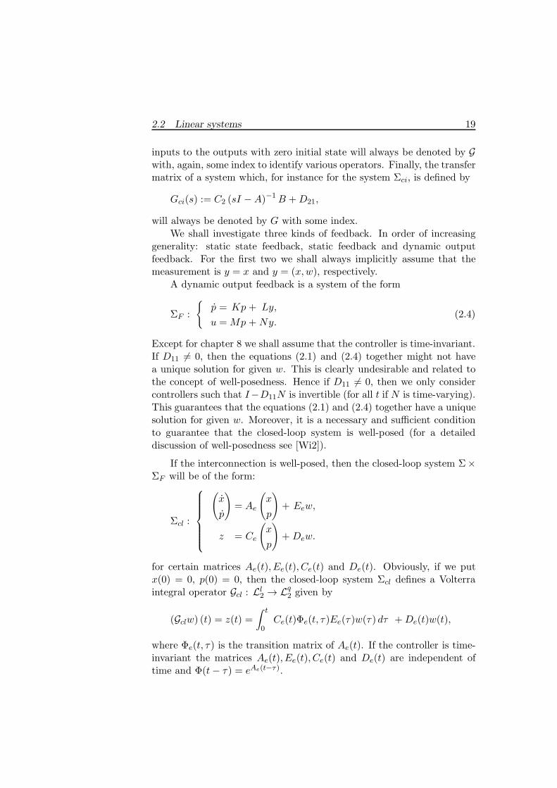
vi Contents
4.7 Invariant zeros on the imaginary axis . . . . . . . . . . . . 844.8 Conclusion . . . . . . . . . . . . . . . . . . . . . . . . . . 89
5 The H∞ control problem with measurement feedback 915.1 Introduction . . . . . . . . . . . . . . . . . . . . . . . . . . 915.2 Problem formulation and main results . . . . . . . . . . . 955.3 Reduction of the original problem to an almost disturbance
decoupling problem . . . . . . . . . . . . . . . . . . . . . . 1005.4 The design of a suitable compensator . . . . . . . . . . . . 1065.5 Characterization of achievable closed-loop systems . . . . 1075.6 No assumptions on any direct-feedthrough matrix . . . . . 1125.7 Conclusion . . . . . . . . . . . . . . . . . . . . . . . . . . 118
6 The singular zero-sum differential game with stability 1206.1 Introduction . . . . . . . . . . . . . . . . . . . . . . . . . . 1206.2 Problem formulation and main results . . . . . . . . . . . 1216.3 Existence of almost equilibria . . . . . . . . . . . . . . . . 1256.4 Necessary conditions for the existence of almost equilibria 1316.5 The regular differential game . . . . . . . . . . . . . . . . 1336.6 Conclusion . . . . . . . . . . . . . . . . . . . . . . . . . . 137
7 The singular minimum entropy H∞ control problem 1397.1 Introduction . . . . . . . . . . . . . . . . . . . . . . . . . . 1397.2 Problem formulation and results . . . . . . . . . . . . . . 1407.3 Properties of the entropy function . . . . . . . . . . . . . 1427.4 A system transformation . . . . . . . . . . . . . . . . . . . 1477.5 (Almost) Disturbance Decoupling and minimum entropy . 1507.6 Conclusion . . . . . . . . . . . . . . . . . . . . . . . . . . 152
8 The finite horizon H∞ control problem 1548.1 Introduction . . . . . . . . . . . . . . . . . . . . . . . . . . 1548.2 Problem formulation and main results . . . . . . . . . . . 1558.3 Completion of the squares . . . . . . . . . . . . . . . . . . 1588.4 Existence of compensators . . . . . . . . . . . . . . . . . . 1628.5 Conclusion . . . . . . . . . . . . . . . . . . . . . . . . . . 165
9 The discrete time full-information H∞ control problem 1669.1 Introduction . . . . . . . . . . . . . . . . . . . . . . . . . . 1669.2 Problem formulation and main results . . . . . . . . . . . 1689.3 Existence of a stabilizing solution of the Riccati equation 1729.4 Sufficient conditions for the existence of suboptimal con-
trollers . . . . . . . . . . . . . . . . . . . . . . . . . . . . . 183

Contents vii
9.5 Discrete algebraic Riccati equations . . . . . . . . . . . . 1869.6 Conclusion . . . . . . . . . . . . . . . . . . . . . . . . . . 189
10 The discrete time H∞ control problem with measurementfeedback 190
10.1 Introduction . . . . . . . . . . . . . . . . . . . . . . . . . . 19010.2 Problem formulation and main results . . . . . . . . . . . 19210.3 A first system transformation . . . . . . . . . . . . . . . . 19510.4 The transformation into a disturbance decoupling problem
with measurement feedback . . . . . . . . . . . . . . . . . 20010.5 Characterization of all suitable controllers and closed-loop
systems . . . . . . . . . . . . . . . . . . . . . . . . . . . . 20210.6 Conclusion . . . . . . . . . . . . . . . . . . . . . . . . . . 204
11 Applications 20511.1 Introduction . . . . . . . . . . . . . . . . . . . . . . . . . . 20511.2 Application of our results to certain robustness problems . 20511.3 Practical applications . . . . . . . . . . . . . . . . . . . . 21411.4 A design example: an inverted pendulum on a cart . . . . 217
12 Conclusion 22612.1 Summary of results obtained . . . . . . . . . . . . . . . . 22612.2 Open problems . . . . . . . . . . . . . . . . . . . . . . . . 23012.3 Conclusion of this book . . . . . . . . . . . . . . . . . . . 233
A Preliminary basis transformations 235A.1 A suitable choice of bases . . . . . . . . . . . . . . . . . . 235A.2 The quadratic matrix inequality . . . . . . . . . . . . . . 243
B Proofs concerning the system transformations 249B.1 Proof of lemma 5.4 . . . . . . . . . . . . . . . . . . . . . . 249B.2 Proof of lemma 5.5 . . . . . . . . . . . . . . . . . . . . . . 252
Bibliography 260
Index 274
Preface
The H∞ norm as a measure has been thoroughly embedded in controltheory during the last few years. Although the H∞ norm has been usedin control for a long time (a concept like bounded real is nothing elsethan an H∞ norm bound), there was a gigantic surge in research effortstowards the minimization of the H∞ norm of the closed loop system inthe last 10 years. A fairly complete solution is now available.
This book tries to bring the reader up to date with respect to the,in our view, most elegant solution to the H∞ control problem: the statespace approach. This book contains numerous references towards otherapproaches to this theory which the reader can use as a starting point forfurther research.
We have tried to start this book at a basic level with the prerequisitesbeing graduate level courses on linear algebra and state space systems.On the other hand, we included the most general solutions available atthe time this book was written. At some times this presented a trade-offand we refer to the literature for the intuition behind some of the abstractconcepts introduced in this book.
This book is the result of my work as a Ph.D. student at the De-partment of Mathematics of Eindhoven University of Technology in theNetherlands from October 1987 until October 1990. Numerous peoplecontributed by assisting me whenever problems arose. In particular, Iwould like to thank Harry Trentelman, Malo Hautus and Ruth Curtain.Clearly they were not the only ones who offered their continuous supportand assistance while preparing this book. The Dutch control communityorganized in the System and Control Theory Network consists of a greatgroup of people. Whomever I asked for a favour or some assistance wasalways willing to help. I would like to thank them all.
Last but not least I would like to thank my family for their moralsupport during these years.
Ann Arbor Anton StoorvogelJuly, 1991
viii

Chapter 1
Introduction
In this book, we study the H∞ control problem. This problem was origi-nally formulated in [Za]. The motivation for this problem should becomeabundantly clear in this book. In this first chapter, we introduce a numberof natural problems whose solutions depend on the results of H∞ control.This chapter will be more or less a justification of the extensive researcheffort in the area of H∞ control, and in particular, why we have writtena book on this subject.
In section 1.1 we formulate and explain the importance of robustnessand, in section 1.2, we sketch very briefly the basic H∞ control problem.The section on robustness outlines the importance of the problems of un-certain systems and the gap metric, which are explained in reasonabledetail in sections 1.3 and 1.4, respectively. These problems are formu-lated with the same objective of improving the robustness although froma completely different point of view and both have a solution which isintimately connected to H∞ control. We shall also explain the mixed-sensitivity problem in this chapter. This is in essence already formulatedas an H∞ control problem and it is practically the only H∞ control pro-blem which has already been applied in practice. To conclude this chapterwe shall outline the H∞ control problems we shall treat in this book.
1.1 Robustness analysis
Control theory is concerned with the control of processes with inputs andoutputs. We would like to know how we can achieve a desired goal wehave for the output of our plant by choosing our inputs.
Example 1.1 : Assume that we have a paper-making machine. Thismachine has certain inputs: wood-pulp, water, pressure and steam. The
1

2 Introduction
wood-pulp is diluted with water. Then the fibres are separated from thewater and a web is formed. Water is pressed out of the mixture and thepaper is then dried on steam-heated cylinders (this is of course a verysimplified view of the process). The product of the plant is the paper.More precisely we have two outputs: the thickness of the paper and themass of fibres per unit area (expressing the quality of the paper). Wewould like both outputs to be equal to some desired value. That is, wehave a process with a number of inputs and two goals: we would like tomake the deviation from the desired values of the thickness and of themass of fibres per unit area of the paper produced as small as possible. ✷
The first step is to find a mathematical model describing the behaviour ofour plant. The second step is to use mathematical tools to find suitableinputs for our plant based on measurements we make of all, or of a subset,of our outputs. However, we apply these inputs to our plant and not toour model. Since our model should be simple enough for the mathemat-ical tools of step 2 (for instance in this book we require that the modelbe linear) the model will not describe the plant exactly. Because we donot know how sensitive our inputs are with respect to the differences be-tween model and plant, the obtained behaviour might differ significantlyfrom the mathematically predicted behaviour. Hence our inputs will ingeneral not be suitable for our plant and the behaviour we obtain can becompletely surprising.
Therefore it is extremely important that, when we search for a controllaw for our model, we keep in mind that our model is far from perfect.This leads to the so-called robustness analysis of our plant and suggestedcontrollers. Robustness of a system says nothing more than that thestability of the system (or another goal we have for the system) willstand against perturbation (structured or unstructured, depending onthe circumstances).
The classic approach to this problem from the 1960s was the LinearQuadratic Gaussian (LQG) theory. In that approach the uncertainty ismodelled as a white noise Gaussian process added as an extra (vector)input to the system. The major problem of this approach is that our un-certainty cannot always be modelled as white noise. While measurementnoise can be quite well described by a random process, this is not thecase with parameter uncertainty. If we model a = 0.9 instead of a = 1,then the error is not random but deterministic. The only problem is thatthe deterministic error is unknown. Another problem of main importancewith parameter uncertainty is that uncertainty in the transfer from inputsto outputs cannot be modelled as state or output disturbances, i.e. extra

1.2 The H∞ control problem 3
inputs. This is due to the fact that the size of the errors is relative to thesize of the inputs and can hence only be modelled as an extra input in anon-linear framework.
In the last few years several approaches to robustness have been stud-ied mainly for one goal: to obtain internal stability, where instead of try-ing to obtain this for one system, it is necessary for a class of systemssimultaneously. It is then hoped that a controller which stabilizes allelements of this class of systems also stabilizes the plant itself.
In this chapter two approaches to this problem will be briefly dis-cussed. Both approaches are in a linear, time-invariant setting and resultin an H∞ control problem.
1.2 The H∞ control problem
We now state the H∞ control problem. Assume that we have a system Σ:
Σ✛y
✛
✛u
✛z w
(1.1)
We assume Σ to be a linear time-invariant system either in continuoustime or in discrete time. We note that Σ is a system with two kindsof inputs and two kinds of outputs. The input w is an exogenous inputrepresenting the disturbance acting on the system. The output z is anoutput of the system, whose dependence on the exogenous input w wewant to minimize. The output y is a measurement we make on the system,which we shall use to choose our input u, which in turn is the tool wehave to minimize the effect of w on z. A constraint we impose is thatthis mapping from y to u should be such that the closed-loop system isinternally stable. This is quite natural since we do not want the states tobecome too large while we try to regulate our performance. The effect ofw on z after closing the loop is measured in terms of the energy and theworst disturbance w. Our measure, which will turn out to be equal to theclosed-loop H∞ norm, is the supremum over all disturbances unequal tozero of the quotient of the energy flowing out of the system and the energyflowing into the system. A more precise definition is given in chapter 2.
Note that this problem formulation in itself does not have any con-nection with robustness.

4 Introduction
Example 1.2 : Assume that we have the following system:
Σ :
x = − u + w,
y = x,
z = u.
It can be checked that a feedback law which minimizes the effect of w onz in the above sense is given by:
u = εx
where ε is a very small positive number. On the other hand it is easily seenthat a small perturbation of the system parameters might yield a closed-loop system which is unstable. Hence for this controller, the internalstability of the closed-loop system is certainly not robust with respect toperturbations of the state matrix. ✷
1.3 Stabilization of uncertain systems
As already mentioned, a method for handling the problem of robustnessis to treat the uncertainty as additional input(s) to the system. The LQGdesign method treats these inputs as white noise and we noted that pa-rameter uncertainty is not suitable for treatment as white noise. Also theidea of treating the error as extra inputs was not suitable because thesize of the error might be relative to the size of the inputs. This yieldsan approach where parameter uncertainty is modelled as a disturbancesystem taking values in some range and modelled in a feedback setting(which allows us to incorporate the “relative” character of the error).We would like to know the effect with respect to stability of the “worst”disturbance in the prescribed parameter range (we want guaranteed per-formance so, even if the worst happens, it should still be acceptable). Ifthis disturbance cannot destabilize the system, then we are certain (underthe assumption that the plant is exactly described by a system we obtainfor some value of the parameters in the prescribed range) that the plantis stabilized by our control law.
It is easy to verify that parameter uncertainty in a linear setting can

1.3 Stabilization of uncertain systems 5
very often be modelled as:
ΣK
Σ✻
✛
❄
✛
z
y u
w (1.2)
Here the system ΣK represents the uncertainty and if the transfermatrix of ΣK is zero, then we obtain our nominal model from u to y. Thesystem ΣK might contain uncertainty of parameters, ignored dynamicsafter model reduction or discarded non-linearities. The goal is to finda feedback law which stabilizes the model for a large range of systemsΣK . In chapter 11 we shall give some examples of different kinds ofuncertainties which can be modelled in the above sense. We shall alsoshow what the results of this book applied to these problems look like.At this point, we only show by means of an example that a large classof parameter uncertainty can be considered as an interconnection of theform (1.2).
Example 1.3 : Assume that we have a single-input, single-output systemwith two unknown parameters:
Σn :
{x = −ax + bu,
y = x.
where a and b are parameters with values in the ranges [a0 − ε, a0 +ε] and [b0 − δ, b0 + δ] respectively. We can consider this system as aninterconnection of the form (1.2) by choosing the system Σ to be equal to:
Σ :
x = −a0x + b0u + w,
y = x,
z =
(10
)x +
(01
)u.
and the system ΣK to be the following static system:
w =(a− a0 b− b0
)z.
It is easily seen that by scaling we may assume that ε = δ = 1. ✷

6 Introduction
If we want to use some special structure of the system ΣK (e.g. that ΣK
is static and not dynamic as in the above example), then we have to resortto the so-called µ-synthesis of J. Doyle (see [Do2, Do3]) or to the (similar)theory of real stability radii (see [Hi]). µ-synthesis has the disadvantagethat this method is so general that, at this moment, no reasonably effi-cient algorithms are available to improve robustness via µ-synthesis. Thesame is true for the related approach of working with real stability radii.The available technique for µ-synthesis is to use an H∞ upper bound (de-pending on scales) for µ which is consequently minimized by choosing anappropriate controller. The result is again minimized over all possiblechoices for the scales.
On the other hand, if we want to find a controller from y to u such thatthe closed-loop system is stable for all stable systems ΣK with H∞ normless than γ, then it has been shown (see [Hi]) that the problem is equiv-alent to the following problem: find a controller which is such that theclosed-loop system (if the transfer matrix of ΣK is zero) is internally sta-ble and the H∞ norm from w to z is strictly less than γ−1. This problemcan be solved using the techniques given in this book.
1.4 The graph topology
When we treat parameter uncertainty as we did in the previous sectionthen we need to know explicitly how this uncertainty is structured in oursystem. In many practical cases we do not have such information and forthese cases a different approach is needed.
We could formulate the problem abstractly as follows: assume thatsome nominal plant is given and some controller stabilizes this plant.Does the same controller also stabilize systems which are “close” to ournominal plant?
The problem in this formulation is how to define the concept of dis-tance between two systems. Since systems are in fact nothing else thaninput–output operators a natural distance concept would be the inducedoperator norm. However, in this case an unstable system must be seen asan unbounded operator and hence this distance concept cannot be usedto define distances between unstable systems. On the other hand, it isquite possible that our plant is unstable and hence we need a conceptof distance which is still valid in the case of one or both of the systemsbeing unstable. The graph topology turns out to yield a useful distanceconcept for these cases.
When do we call two systems close to each other? Firstly, if we havea controller which internally stabilizes one system, then it should also

1.4 The graph topology 7
be internally stabilizing for the other system. Secondly, if we apply thesame stabilizing controller to each one of the systems, then the closed-loopsystems should be close to each other, measured in the induced operatornorm. Note that both closed-loop systems are stable and hence thisoperator norm is always finite. The first requirement is natural becausewe consider robustness of internal stability. The second requirement isadded because we would like to prevent other performance criteria frombeing highly sensitive to perturbations even though stability is preserved.
Next, we shall formalize the above intuitive reasoning. We define thegraph topology for the set of linear time-invariant and finite-dimensionalsystems. A sequence of systems {Σn} is said to converge to Σ in thegraph-topology if the following holds:
• For every controller ΣF which stabilizes Σ, there exists a naturalnumber N such that for all n > N , the controller ΣF internallystabilizes Σn.
• For every controller ΣF which stabilizes Σ denote the closed-loopoperator by GF and the closed-loop operator obtained by applyingΣF to Σn by GF,n. Then
‖GF − GF,n‖∞ → 0 as n→∞.
Here ‖ · ‖∞ denotes the induced operator norm which will be formallydefined in section 2.5.
The graph topology has been introduced in [Vi]. In [Zh] it was shownthat this topology is always equal to the gap topology (in [Zh] this is alsoshown for more general classes of infinite-dimensional systems). The gaptopology is yet another topology that can be applied to define conver-gence between possibly unstable plants. However, the gap topology ismetrizable and hence we can now really discuss the distance between twoplants. Note that the concept of coprime-factor perturbations as used in[Gl4, MF] again yields the same topology (see [Vi], in [GS] it was shownthat the gap metric is related to so-called normalized coprime-factor per-turbations).
Now, the problem of finding a maximally robust controller in thissetting is defined as follows: for each internally stabilizing controller ofthe nominal plant we search for the distance to the nearest system inthe gap metric which is not stabilized by our controller. This is calledthe stability margin of the controller. Finally we search for the controllerwith the largest stability margin. The above problem has been reducedin [GS, Hab, Zh] to an H∞ control problem.

8 Introduction
1.5 The mixed-sensitivity problem
The mixed-sensitivity problem is a special kind of H∞ control problem.In the mixed-sensitivity problem it is assumed that the system underconsideration can be written as the following interconnection where ΣF
is the controller which has to satisfy certain prerequisites.
ΣF
ΣW1
Σ
ΣV
ΣW2✲ ✲
✻✲
✻
✻
✲
❄
❄ ✲ ✲
z1 w
wyur z2+
− +
+◦ ◦(1.3)
ManyH∞ control problems can be formulated in terms of an intercon-nection of the form (1.3). We shall show as an example how the trackingproblem can be formulated in the setting described by the diagram (1.3).We first look at the following interconnection:
ΣF Σ✲ ✲✻
✲ ✲yur +
−◦ (1.4)
The problem is to regulate the output y of the system Σ to look likesome given reference signal r by designing a precompensator ΣF whichhas as its input the error signal, i.e. the input of the controller is thedifference between the output y of Σ and the reference signal r. To preventundesirable surprises we require internal stability. We could formulate theproblem as “minimizing” the transfer function from r to r − y. As onemight expect we shall minimize the H∞ norm of this transfer functionunder the constraint of internal stability. The transfer matrix from r tou should also be under consideration. In practice the process inputs willoften be restricted by physical constraints. This yields a bound on thetransfer matrix from r to u. These transfer matrices from r to r − y and

1.5 The mixed-sensitivity problem 9
from r to u are given by:
S := (I +GGF )−1 ,
T := GF (I +GGF )−1 ,
respectively, where G and GF denote the transfer matrices of Σ and ΣF .Here S is called the sensitivity function and T is called the control sen-sitivity function. A small function S expresses good tracking propertieswhile a small function T expresses small inputs u. Note that there isa trade-off: making S smaller will in general make T larger. We add asignal w to the output y as in (1.3). Then the transfer matrix from w toy is equal to the sensitivity matrix S and the transfer matrix from w tou is equal to the control sensitivity matrix T .
As noted in section 1.2 the H∞ norm can be viewed as the maximumamount of energy coming out of the system, subject to inputs with unitenergy. However, if we apply the Laplace transform, then we obtain afrequency-domain characterization. For a single-input, single-output sta-ble system the H∞ norm is equal to the largest distance of a point on theNyquist contour to the origin. Hence the H∞ norm is a uniform boundover all frequencies on the transfer function. Although we assume thetracking signal to be, a priori, unknown, it might be that we know thatour tracking signal will have a limited frequency spectrum. It is in gen-eral impossible to track signals of very high frequency reasonably well.On the other hand, since in general the model is only accurate up to acertain frequency, since we have bandwidth limitations on actuators andsensors and since we have problems implementing controllers with a largebandwidth, we only require the system to track signals of frequencies upto a certain bandwidth. In this situation straightforward application ofH∞ control might yield bad results because it only investigates a uni-form bound over all frequencies. Also, certain frequencies may be moreimportant than others for the error signal and the control input.
Thus in diagram (1.3), the systems ΣW1, ΣW2 and ΣV are weightswhich are chosen in such a way that we put more effort in regulatingfrequencies of interest than one uniform bound. For practical purposes thechoice of these weights is extremely important. For single-input, single-output systems expressing performance criteria into requirements on thedesired shape of the magnitude Bode diagram is well established (see, e.g.[FL, Hor]). This immediately translates into the appropriate choice forthe weights. On the other hand, for multi-input, multi-output systems itis in general very hard to translate practical performance criteria into anappropriate choice for the weights. It should be noted that in practicalcircumstances it is often better to minimize the integrated tracking error

10 Introduction
as we do in section 11.4 (this forces a zero steady-state tracking error).This can also be incorporated in the weights and is simply one way toemphasize our interest in tracking signals of low frequency.
In this way, we obtain the interconnection (1.3). Note that the trans-fer matrix from the disturbance w to z1 and z2 is(
GW1TGV
GW2SGV
)(1.5)
where GW1, GW2 and GV are the transfer matrices of ΣW1, ΣW2 and ΣV ,respectively. Note that we can also use these weights to stress the relativeimportance of minimizing the sensitivity matrix S with respect to theimportance of minimizing the control sensitivity matrix T by multiplyingGW1 by a scalar.
We want to find a controller which minimizes the H∞ norm of thetransfer matrix (1.5) and which yields internal stability. This problemcan be solved using the techniques we present in this book.
1.6 Main items of this book
As already mentioned, this book will deal with several aspects of H∞ con-trol. In recent years many papers have been published on this subjectand, in this section, we want to describe briefly the new contributions thisbook makes to the existing theory. We shall consider the time-domainapproach to H∞ control, which has received a large impulse from thepaper [Do5]. This book is self-contained but we will put emphasis on thefollowing aspects of the time-domain approach to H∞ control:
• Singular systems
• Differential games
• The finite horizon H∞ control problem
• The minimum entropy H∞ control problem
• Discrete time systems.
First we introduce some notation and give some preliminary results inchapter 2. In chapter 3, we give some results on the state feedbackH∞ control problem of which the main results were already basicallyknown in the literature. We have added this chapter for the sake ofcompleteness and in order to have the results available for the rest of thebook. In chapters 4 and 5 we extend the known H∞ theory to so-called

1.6 Main items of this book 11
singular systems. In chapter 6 we discuss the differential game and its re-lation toH∞ control. Next, in chapter 7, we discuss the minimum entropyH∞ control problem. In chapter 8 we study the finite horizon H∞ controlproblem. Then, in chapters 9 and 10, we investigate the H∞ control pro-blem for discrete time systems. In chapter 11 we will apply the derivedtheory to find results for several robust stabilization problems. We willalso give a worked-out design example of an inverted pendulum on a cart.Finally chapter 12 contains a number of concluding remarks. AppendixA gives the details of the state decomposition on which the proofs of ourresults for singular systems are based. Appendix B contains the proofsof two technical lemmas from chapter 5.
We shall discuss the main subjects of this book in some detail in thenext five subsections.
1.6.1 Singular systems
In the paper [Do5] linear finite-dimensional time-invariant systems wereconsidered which satisfy two kinds of essential assumptions:
• The subsystem from the control input to the output should not haveinvariant zeros on the imaginary axis and its direct-feedthroughmatrix should be injective.
• The subsystem from the disturbance to the measurement should nothave invariant zeros on the imaginary axis and its direct-feedthroughmatrix should be surjective.
Invariant zeros are defined in chapter 2. For the moment it suffices tothink of invariant zeros as points in the complex plane where the transfermatrix loses rank.
Throughout this book we shall make the same assumption with res-pect to invariant zeros, by excluding invariant zeros on the imaginary axisfor both subsystems. A discussion of the difficulty of invariant zeros onthe imaginary axis is given in chapter 12.
We define singular systems (contrary to regular systems) to be sys-tems which do not satisfy at least one of the two above assumptions onthe direct-feedthrough matrices. In chapters 4 and 5 we shall extend theresults from [Do5] to the class of singular systems.
These singular systems are more difficult to analyse. In the case thatthe direct-feedthrough matrix from the control input to the output is notinjective then either the system has an invariant zero at infinity or thesubsystem from the control input to the output is not injective.

12 Introduction
• An invariant zero at infinity. This is as difficult as invariantzeros on the imaginary axis. The problems with invariant zeroson the imaginary axis are explained in chapter 12. Basically themethod of handling an invariant zero is to choose a controller whichcreates a pole in the same point. Then the invariant zero is cancelledvia pole-zero cancellation. Because of our requirement of internalstability this is only possible for invariant zeros in the open left halfplane. For invariant zeros in the open right half plane it is clearlynot possible. In the case of an invariant zero on the imaginary axiswe can achieve this cancellation approximately by creating a polein the left half plane which is very close to the imaginary axis. Atreatment like this for invariant zeros on the imaginary axis is givenin [HSK]. At the moment we are only interested in invariant zerosat infinity. In general, the so-called central controller (as givenin section 5.5) will be non-proper in this case. Hence we indeedhave a pole in infinity which “cancels” our invariant zero at infinity.However, it will turn out that we can approximate this controllerby a proper controller. It will be shown that the problem of thisapproximation can be reduced to the problem of almost disturbancedecoupling. In this problem one is looking for conditions underwhich we can find internally stabilizing controllers which make theH∞ norm arbitrarily small. Since this problem has been solved in[OSS1, OSS2, Tr, WW] we were able to use these results.
• The system from the control input to the output is notinjective. This implies that there are several inputs which havethe same effect on the output. Using a geometric approach thisnon-uniqueness can be filtered out. This is done explicitly in [S2].We do the same in this book but more implicitly because we handleinvariant zeros at infinity at the same time.
On the other hand, the subsystem from the disturbance to the measure-ment might not be surjective. The problems related to this fact play acompletely dual role and we shall tackle these problems by relating themto the problems of a dual system.
In [Do5] necessary and sufficient conditions are given for regular sys-tems under which the existence of an internally stabilizing controllerwhich makes the H∞ norm less than some, a priori given, number γ > 0is guaranteed. These conditions are in terms of two algebraic Riccatiequations. For singular systems these Riccati equations will be replacedby quadratic matrix inequalities. This is completely analogous to LinearQuadratic (LQ) optimal control where for singular systems the role of the

1.6 Main items of this book 13
algebraic Riccati equation is replaced by a linear matrix inequality.Finally, a few words about the interest in singular systems. First of
all, for mathematicians removing annoying assumptions is always of inter-est. Moreover, singular systems do arise in natural control problems, forexample the problem of treating parameter uncertainty via the methoddiscussed in section 1.3 will often yield H∞ control problems for singularsystems. This is worked out in more detail in chapter 12. Another exam-ple is the problem of Loop Transfer Recovery (see [Ni]) which also yieldsH∞ control problems for singular systems.
Another reason for looking at singular systems is the omnipresentrequirement of reduced-order controllers. By assuming that k states areobserved without noise, it can be shown that the dynamic order of thecontroller can be reduced by k. However, to show this property we needto use singular systems (see [St13]).
Finally, a major reason for looking at singular systems is that quiteoften in applications direct-feedthrough matrices appear which are nearlysingular. The results of [Do5] may still be applied but for deriving numer-ically reliable algorithms it is useful to know exactly what will happen ifthe direct-feedthrough matrices are no longer injective or surjective.
1.6.2 Differential game
As we mentioned in the previous subsection, the conditions under whichwe can make the H∞ norm less than some, a priori given, number, areeither in terms of the solutions of two algebraic Riccati equations or interms of the solutions of two quadratic matrix inequalities. The solutionsof these equations or inequalities have no direct meaning in H∞ control.On the other hand, it would be good for the overall picture if we couldunderstand the role of these solutions better.
We shall try to achieve this in chapter 6 for a special case. Firstof all we assume that we have a continuous time system. Secondly weonly investigate the special case of state-feedback. In chapters 3 and 4 itwill be shown that in this case we have only one Riccati equation or onequadratic matrix inequality.
It turns out that the theory of differential games yields the desiredunderstanding of the role of the solution of either equation or inequality.The quadratic form associated with the solution of our Riccati equationturns out to be a Nash equilibrium for a differential game with a specialcost criterion. The quadratic form associated with the solution of ourquadratic matrix inequality turns out to be an almost Nash equilibriumfor a differential game with the same cost criterion.
It is shown that being able to make the H∞ norm strictly less than

14 Introduction
our, a priori given, bound γ is a sufficient condition for the existence ofan almost Nash equilibrium. On the other hand, being able to make theH∞ norm less than or equal to γ is a necessary condition for the existenceof an almost Nash equilibrium. Note that the cost criterion explicitlydepends on our bound γ.
1.6.3 The minimum entropy H∞ control problem
Besides robustness we often require controllers to yield a satisfactory per-formance. Therefore if we model uncertainty as we did in section 1.3 thenwe might have the following interconnection:
Σ
ΣK
✛z2
✛
✛
✛ ✛
✲ ✲
w2
✛y u
z1 w1
(1.6)
We assume that uncertainty is affecting the given system Σ via the un-known system ΣK and we want to achieve a certain level of robustnesswith respect to internal stability and simultanuously attain a certain per-formance on the transfer matrix from w1 to z1. The latter performancerequirement will be assumed to be the minimization of a quadratic perfor-mance criterion (which can be expressed in terms of the H2 norm, definedin the next chapter, of the closed-loop transfer matrix by adding suitableweighting). Other criteria might be suitable and are interesting openproblems for future research.
The above goal can be translated into the following objective: finda controller from y to u such that the closed-loop system is internallystable, the closed-loop transfer matrix from w2 to z2 has H∞ norm lessthan some, a priori given, number γ and the H2 norm of the closed-looptransfer matrix from w1 to z1 is minimized over all controllers whichsatisfy the first two conditions.
The above problem is still a completely unsolved problem. To simplifythe problem the H2 norm is replaced by an auxiliary cost function. This

1.6 Main items of this book 15
auxiliary cost function is an upper bound for the H2 norm and it is hopedthat by minimizing this auxiliary cost function instead of the H2 norm westill get a satisfactory performance.
The above problem has been investigated in [Mu] for regular systemsunder the assumption that z1 = z2 and w1 = w2. In general this auxiliarycost function is not very intuitive but in this special case we can replaceit by an entropy function which yields more insight. In literature moregeneral cases have been investigated (see [BH2, HB, HB2, RK]) and itremains an active research area. In this book we will investigate thespecial case z1 = z2 and w1 = w2 for singular systems. Our proofs areself-contained and in our opinion more straightforward then the proofsgiven in [Mu].
1.6.4 The finite horizon H∞ control problem
As already remarked in section 1.2 the H∞ control problem is concernedwith minimizing the H∞ norm. The H∞ norm is equal to the maximumover all disturbances w of the quotient of the amount of energy going intothe system and the amount of energy coming out of this system. In thestandard H∞ control problem, this energy is measured over an infinitetime interval [0,∞). This might not always be realistic in practical appli-cations. Therefore, in the finite horizon H∞ control problem we minimizethe same norm except that the energy is measured over a finite time in-terval [0, T ] for some given T > 0. This problem was solved for regularsystems in [Li5]. We will extend these results to singular systems.
1.6.5 Discrete time systems
Early results for the H∞ control problem were derived for the continuoustime case. In the first chapters of this book we shall only concern ourselveswith continuous time systems. However, in practical applications one isoften concerned with discrete time systems.
One major reason is that to control a continuous time system oneoften applies a digital computer on which we can only implement a dis-crete time controller. One possible approach is to derive a continuoustime H∞ controller and then discretize the controller to be able to useyour computer. This approach is followed in papers like [KA].
A direct digital design where a sample and hold function of givenbandwidth are already incorporated into the plant (so-called sampled-data systems) and we design a discrete time controller for this system isa much better way to discover the limitations of our design. Althoughbasically a much harder problem, major steps forward have been made

16 Introduction
(see [Ch, Ch2, KH, SK]). In these papers the problem is reduced to adiscrete time H∞ control problem of which a solution is therefore needed.
Also, certain systems are in themselves inherently discrete and cer-tainly for these systems it is useful to have results available forH∞ controlproblems.
One approach to solve the discrete time H∞ control problem, is toapply a transformation in the frequency-domain which transforms dis-crete time systems to continuous time systems. The transformation wehave in mind is for instance discussed in [Gen, appendix 1]. With thistransformation discrete time H∞ functions are mapped isometrically ontocontinuous time H∞ functions. One can then use the results available forcontinuous time systems and afterwards apply the inverse transformationon the controller thus obtained.
However, this transformation is not always attractive. It maps sys-tems with a pole in 1 into non-proper systems. Also it clouds the un-derstanding of specific features of discrete time H∞ control because of itscomplexity. If it is possible to derive results for discrete time systems,why not apply these results directly instead of performing this unnaturaltransformation. Another problem is that the state feedback H∞ controlproblem is transformed into a continuous time measurement feedbackH∞ control problem where indeed one might have problems observing thestate. This prevents an understanding of discrete time H∞ controllers asan interconnection of a state feedback and an observer since this distinc-tion is scrambled by the transformation.
Therefore, in chapters 9 and 10 we shall derive results for the discretetime state feedback H∞ control problem and the discrete time measure-ment feedback H∞ control problem, respectively. We shall only considerdiscrete time analogues of regular systems, and hence it might not be toosurprising that our conditions are formulated in terms of discrete timealgebraic Riccati equations.

Chapter 2
Notation and basic properties
2.1 Introduction
In this chapter we introduce the notation and definitions we shall usethroughout this book. Moreover, we give a number of basic propertieswe shall need further on. Most of these properties will not be provenhere but we shall give appropriate references. In this book we deal withboth discrete time systems as well as continuous time systems. Therefore,two sections of this chapter are split up into a discrete time part and acontinuous time part in order to emphasize the differences. While readingthis book, one should always keep in mind that we want to minimize theoutput with respect to the worst case disturbance. This goal is all wewant to achieve and we shall try to achieve it under several differentcircumstances.
Let R denote the real numbers, C denote the complex numbers andlet N denote the non-negative integers. Let C+ (C0, C−) denote the setof all s ∈ C such that Re s > 0 (Re s = 0, Re s < 0). Finally by D (δD,D+) we denote the set of all s ∈ C such that |s| < 1 (|s| = 1, |s| > 1).
2.2 Linear systems
2.2.1 Continuous time
Except for chapters 9 and 10 we shall investigate systems with continuoustime. These systems are described by a differential equation and twooutput equations.
Σ :
x = Ax + Bu + Ew,
y = C1x + D11u + D12w,
z = C2x + D21u + D22w.
(2.1)
17

18 Notation and basic properties
We shall always assume that x, u,w, y and z take values in finite-dimension-al vector spaces: x(t) ∈ Rn, u(t) ∈ Rm, w(t) ∈ Rl, y(t) ∈ Rq andz(t) ∈ Rp. The system parameters A, B, E, C1, C2, D11, D12, D21 andD22 are matrices of appropriate dimensions. We assume that the systemis time-invariant, i.e. the system parameters are independent of time. Ex-cept when stated explicitly, we shall always assume that the initial stateis zero, i.e. x(0) = 0. The input w is the disturbance working on thesystem, whose effect on one of the outputs we want to minimize. Theinput u is the control which we use to achieve this goal. The output yis the measurement on the basis of which we choose our input u. Theoutput z is the output we want to make small relative to the size of thedisturbance w. More precisely, we are searching for a feedback from y tou, denoted by ΣF , such that the closed-loop system Σ×ΣF mapping w toz has a small induced norm. If all information on the system is availablefor feedback, i.e. y = (x,w), or if the state is available for feedback, i.e.y = x, then we shall often delete the second equation in (2.1).
In several chapters the indices of the C- and D-matrices are differentfrom the indices used in system (2.1). This is done to simplify the no-tation in the respective chapters. When comparing results from differentchapters the reader should be careful whether these differences arise ornot.
When we apply an input u and a disturbance w with initial conditionx(0) = ξ then we shall denote by xu,w,ξ and zu,w,ξ the state and theoutput of system (2.1), respectively. In the case that we have zero initialcondition we shall write xu,w and zu,w instead of xu,w,0 and zu,w,0.
Quite often, we shall look at two special subsystems, one in which werestrict attention to the system from u to z:
Σci :
{x = Ax + Bu,
z = C2x + D21u,(2.2)
and one in which we restrict attention to the system from w to y:
Σdi :
{x = Ax + Ew,
y = C1x + D12w.(2.3)
If we only have one input and one output, as in the above two systems,then we can associate with a system the quadruple of the four system pa-rameters. For the sake of simplicity we shall often write, for instance, thesystem (A,B,C2,D21) when, formally, we should write down the systemequations (2.2).
The system equations will always be denoted by a Σ with some indexto identify different systems. The input–output operator mapping the
2.2 Linear systems 19
inputs to the outputs with zero initial state will always be denoted by Gwith, again, some index to identify various operators. Finally, the transfermatrix of a system which, for instance for the system Σci, is defined by
Gci(s) := C2 (sI −A)−1B +D21,
will always be denoted by G with some index.We shall investigate three kinds of feedback. In order of increasing
generality: static state feedback, static feedback and dynamic outputfeedback. For the first two we shall always implicitly assume that themeasurement is y = x and y = (x,w), respectively.
A dynamic output feedback is a system of the form
ΣF :
{p = Kp + Ly,
u =Mp + Ny.(2.4)
Except for chapter 8 we shall assume that the controller is time-invariant.If D11 �= 0, then the equations (2.1) and (2.4) together might not havea unique solution for given w. This is clearly undesirable and related tothe concept of well-posedness. Hence if D11 �= 0, then we only considercontrollers such that I−D11N is invertible (for all t if N is time-varying).This guarantees that the equations (2.1) and (2.4) together have a uniquesolution for given w. Moreover, it is a necessary and sufficient conditionto guarantee that the closed-loop system is well-posed (for a detaileddiscussion of well-posedness see [Wi2]).
If the interconnection is well-posed, then the closed-loop system Σ×ΣF will be of the form:
Σcl :
(x
p
)= Ae
(x
p
)+ Eew,
z = Ce
(x
p
)+ Dew.
for certain matrices Ae(t), Ee(t), Ce(t) and De(t). Obviously, if we putx(0) = 0, p(0) = 0, then the closed-loop system Σcl defines a Volterraintegral operator Gcl : Ll2 → Lq2 given by
(Gclw) (t) = z(t) =∫ t
0Ce(t)Φe(t, τ)Ee(τ)w(τ) dτ +De(t)w(t),
where Φe(t, τ) is the transition matrix of Ae(t). If the controller is time-invariant the matrices Ae(t), Ee(t), Ce(t) and De(t) are independent oftime and Φ(t− τ) = eAe(t−τ).

20 Notation and basic properties
If the interconnection is well-posed, then it is called internally stableif, with w = 0, for every initial state of the system and every initial stateof the controller the state of the system and the state of the controller inthe interconnection converge to zero as t→∞. If the controller is givenby (2.4) and the system is given by (2.1), then this is equivalent to therequirement that the matrix(
A+BN(I −D11N)−1C1 B(I −ND11)−1M
L(I −D11N)−1C1 K + L(I −D11N)−1D11M
)(2.5)
be asymptotically stable, i.e. all its eigenvalues lie in the open left halfcomplex plane. For systems with discrete time, asymptotic stability willhave a different meaning (see the next subsection). Moreover, note thatif D11 = 0, then the interconnection is always well-posed. In that casethe matrix (2.5) simplifies considerably and is equal to(
A+BNC1 BM
LC1 K
). (2.6)
For a finite-dimensional system (A,B,C,D) we shall call the matrix Athe state matrix of the system. Accordingly, the matrix (2.5) or (2.6)will be referred to as the closed-loop state matrix. We shall call B theinput matrix, C the output matrix and D the direct-feedthrough matrix.Finally, the dimension of the state space is called the McMillan degree ofthe realization.
After applying the compensator ΣF described by the static feedbacklaw u = F1x+ F2w the closed-loop transfer matrix is given by
GF (s) := (C2 +D21F1) (sI −A−BF1)−1 (E +BF2) + (D22 +D21F2) .
(2.7)
Just as for dynamic compensators, the closed-loop system is called inter-nally stable if, with w = 0 and for all initial states, the state converges tozero as t→∞. It is easy to check that the closed-loop system is internallystable if, and only if, the matrix A+BF1 is asymptotically stable. Thiscan also be derived from the dynamic feedback case discussed above bynoting that
y =
(I
0
)x+
(0I
)w
and that the matrix (2.6) then becomes equal to A + BF1. Here K is a0× 0 matrix and hence disappears and N = ( F1 F2 ). A compensator

2.2 Linear systems 21
described by a static state feedback law u = Fx can be considered as aspecial case of a static feedback law and the above definitions will be usedcorrespondingly.
We shall say that matrices P and Q satisfy dual properties if Psatisfies a certain property for the system (2.1) if, and only if, QT satisfiesthe same property for the dual system defined by
ΣT :
x = ATx + CT
1 u + CT2w,
y = BTx + DT11u + DT
21w,
z = ETx + DT12u + DT
22w.
2.2.2 Discrete time
In chapters 9 and 10 we shall investigate systems with discrete time.These systems are described by a difference equation and two outputequations.
Σ :
σx = Ax + Bu + Ew,
y = C1x + D11u + D12w,
z = C2x + D21u + D22w.
(2.8)
where σ denotes the shift-operator, which is defined by
(σx) (k) := x(k + 1).
We shall only investigate shift-invariant systems, i.e. we assume through-out that the system parameters do not depend on time. All assumptionsand definitions for continuous time as given in the previous subsectionhave an analogous meaning in discrete time. However, one point has tobe discussed explicitly.
A dynamic output feedback is a system of the form
ΣF :
{σp = Kp + Ly,
u =Mp + Ny.(2.9)
As in the previous section we define the interconnection to be internallystable if the interconnection is well-posed and if, with w = 0, for everyinitial state of the system and for every initial state of the controller thestate of the system and the state of the controller in the interconnectionconverge to zero as t → ∞. If the controller is given by (2.9) and thesystem is given by (2.8) then this is equivalent to the requirement thatthe matrix (2.5) is asymptotically stable, i.e. all its eigenvalues lie in theopen unit disc. Note that for systems with continuous time asymptotic

22 Notation and basic properties
stability of a matrix has a different meaning. That is, we still have thesame matrix as in the continuous time case only this time its eigenvaluesshould be in the open unit disc instead of the open left half plane.
Later on we shall also need a backwards difference equation of theform
σ−1x = Ax + Bu.
A function x fromN∪{−1} toRn is said to be a solution of this backwardsdifference equation if
x(k − 1) = Ax(k) +Bu(k),
for all k ∈ N .
2.3 Rational matrices
In this section we recall some basic notions on rational matrices whichare either applied to system matrices (which will be defined on the nextpage) or transfer matrices.
Let R[s] denote the ring of polynomials with real coefficients. LetRn×m[s] be the set of all n × m matrices with coefficients in R[s]. Anelement of Rn×m[s] is called a polynomial matrix. Linear polynomialmatrices of the form sE − F are sometimes called a matrix pencil. R(s)denotes the field of rational functions with real coefficients, i.e. R(s) isthe quotient field of R[s]. Let Rn×m(s) be the set of all n ×m matriceswith coefficients in R(s).
An element of Rn×m(s) is called a rational matrix. A rational ma-trix G is called stable if G has no poles in the closed right half complexplane. G is called proper if lims→∞G(s) exists, and strictly proper if thislimit is zero. Moreover, for a given proper rational matrix G, the ma-trix lims→∞G(s) is called the direct-feedthrough matrix. Note that thedirect-feedthrough matrix of a system is equal to the direct-feedthroughmatrix of its transfer matrix.
By rankK we denote the rank of a matrix as a matrix with entries inthe field K. We shall often write only rank in the case that K = R orK = C (note that for a real matrix the rank over C always equals its rankover R). Moreover, we often use the term normal rank for rankK whereK = R(s).
We shall first discuss a number of properties of polynomial matrices.A square polynomial matrix is called unimodular if it is invertible overthe ring of polynomial matrices. Two polynomial matrices P and Q arecalled unimodularly equivalent if unimodular matrices U and V exist

2.3 Rational matrices 23
such that Q = UPV . In this book, we denote the fact that P and Q areunimodularly equivalent by P ∼ Q. It is well known (see [Ga]) that forany P ∈ Rn×m[s] there exists Ψ ∈ Rn×m[s] of the form
Ψ =
ψ1 0 · · · 0 0 · · · 0
0. . .
. . ....
.
.....
.
... . .
. . . 0 0 · · · 0
0 · · · 0 ψr 0 · · · 0
0 · · · 0 0 0 · · · 0
......
......
...
0 · · · 0 0 0 · · · 0
such that P ∼ Ψ. Here ψi are monic polynomials with the property thatψi divides ψi+1 for i = 1, . . . , r − 1.
The polynomial matrix Ψ is called the Smith form of P (see [Ga]).The polynomials ψi are called the invariant factors of P . Their productψ = ψ1ψ2 · · ·ψr is called the zero polynomial of P . The roots of ψ arecalled the zeros of P . The integer r is equal to the normal rank of Pas defined before. If s is a complex number, then P (s) is an element ofCn×m. It is easy to see that rankR(s)P = rank P (s) for all s ∈ C if, andonly if, P is unimodularly equivalent to the constant n×m matrix(
Ir 00 0
),
where Ir is the r × r identity matrix.Next we recall some important facts on the structure of a linear sys-
tem Σci = (A,B,C,D). The (Rosenbrock) system matrix of Σci is definedas the polynomial matrix
Pci :=
(sI −A −BC D
).
The invariant factors of Pci are called the transmission polynomials ofΣci. The transmission polynomials unequal to 1 are called the non-trivialtransmission polynomials of Pci. The zeros of Pci are called the invariantzeros of Σci. Clearly, s ∈ C is an invariant zero of Σci if, and only if,
rankPci(s) < rankR(s)Pci.
This concept of invariant zeros (see e.g. [Ro]) will play an important rolein this book.
It is easy to see that if F ∈ Rm×n and if Pci,F is the system matrixof Σci,F := (A+BF,B,C +DF,D), then Pci ∼ Pci,F . In particular, this

24 Notation and basic properties
implies that the transmission polynomials of Σci and Σci,F coincide and,a fortiori, that the invariant zeros of Σci and Σci,F coincide.
We can also associate with the system Σci the controllability pencil
L(s) :=(sI −A −B
),
and the observability pencil
M(s) :=
(sI −AC
).
A special case which is often investigated in H∞ control theory is thecase that D is injective and CTD = 0. In which case the invariant zerosof Σci are the zeros of M . That is, the invariant zeros of Σci are theunobservable eigenvalues of (C,A).
A system Σci = (A,B,C,D) is called left- (right-) invertible if thetransfer matrix of Σci is left- (right-) invertible as a rational matrix. Thisis equivalent to the requirement that the system matrix of Σci be left-(right-) invertible as a rational matrix. It can be shown that a system isleft-invertible if, and only if, the input–output operator associated withthis system is injective. However, it is in general not true that right-invertibility implies surjectivity of the input–output operator. We definethe class of functions C∞
0 as the class of infinitely often differentiablefunctions on [0,∞) such that all derivatives are equal to zero in zero.Then the continuous time system Σci is right-invertible if, and only if,the input–output operator as a map from C∞
0 to C∞0 is surjective. A
discrete time system is right-invertible if all sequences f with f(0) =f(1) = . . . = f(n) = 0 are contained in the image of the input–outputoperator. Here n is equal to the dimension of the state space.
2.4 Geometric theory
In this section we recall some basic notions from the geometric approachto linear system theory. We shall use the geometric approach only forcontinuous time systems and one should note that although we could usethe geometric approach for discrete time systems too, its usefulness forour problems is mainly restricted to continuous time systems.
We first introduce the important concepts of controlled invarianceand conditioned invariance (see [SH, Wo]).

2.4 Geometric theory 25
Definition 2.1 : A subspace V of Rn is said to be A-invariant if AV ⊆ V.A subspace V of Rn is said to be conditioned invariant (also called (C,A)-invariant) if a linear mapping G exists such that
(A+GC)V ⊆ V.
A subspace V of Rn is said to be controlled invariant (also called (A,B)-invariant) if a linear mapping F exists such that
(A+BF )V ⊆ V. ✷
Note that the alternative terminology of (C,A)-invariant and (A,B)-in-variant is such that the only difference in the terminology for these twoconcepts is the order of the matrices. One has to remember that thesetwo properties are in fact associated to the system (A,B,C, 0) where(A,B)-invariance means that a state feedback F exists which makes thesubspace V invariant under the closed-loop state matrix A + BF while(C,A)-invariance means that an output injection G exists which makesthis subspace invariant under the state matrix A+GC. Finally, we wouldlike to remark that these properties are dual to each other: V is (C,A)-invariant if, and only if, V⊥ is (AT, CT)-invariant.
The following well-known lemma is a convenient tool for checkingwhether these properties hold for a certain subspace (see [SH, Wo]).
Lemma 2.2 : A subspace V of Rn is (C,A)-invariant if, and only if,
A (V ∩ kerC) ⊆ V.
A subspace V of Rn is (A,B)-invariant if, and only if,
AV ⊆ V + imB. ✷
We now define a number of particular linear subspaces of the state space,among which is the strongly controllable subspace. The latter will play akey role throughout this book.
Definition 2.3 : Consider the system
Σci :
{x = Ax + Bu,
z = Cx + Du.(2.10)

26 Notation and basic properties
We define the strongly controllable subspace T (Σci) as the smallest sub-space T of Rn for which a linear mapping G exists such that:
(A+GC)T ⊆ T , (2.11)Im (B +GD) ⊆ T . (2.12)
We also define the detectable strongly controllable subspace Tg(Σci) as thesmallest subspace T of Rn for which a linear mapping G exists such that(2.11) and (2.12) are satisfied and moreover A + GC |Rn/T is asymp-totically stable.
A system is called strongly controllable if its strongly controllable sub-space is equal to the whole state space. ✷
We also define the dual versions of these subspaces:
Definition 2.4 : Consider the system (2.10). We define the weakly un-observable subspace V(Σci) as the largest subspace V of Rn for which amapping F exists such that:
(A+BF )V ⊆ V, (2.13)(C +DF )V = {0}. (2.14)
We also define the stabilizable weakly unobservable subspace Vg(Σci) asthe largest subspace V for which a mapping F exists such that (2.13) and(2.14) are satisfied and moreover A+BF | V is asymptotically stable.
A system is called strongly observable if its weakly unobservable sub-space is equal to {0}. ✷
We can give intuitive interpretations of these subspaces. V(Σci) is thesubspace of all x0 ∈ Rn such that for the system (2.10) with initialcondition x(0) = x0 there exists an input function u on [0,∞) such thatthe output function y of the system is identical zero on [0,∞). Vg(Σci)has the same interpretation but with the extra constraint on the input uthat the resulting state trajectory x(t) converges to 0 as t→∞.
On the other hand, T (Σci) consists of all x0 ∈ Rn such that for thesystem (2.10) with initial condition x(0) = x0 and for all ε > 0 thereexist T > 0 and an input function u such that the resulting state satisfiesx(T ) = 0 while the L1-norm of the output y is less than ε, i.e. we cansteer the initial state x0 to 0 in finite time and, at the same time, we canmake the L1-norm of the output y arbitrarily small. An interpretation

2.4 Geometric theory 27
of Tg(Σci) can be given in terms of observers but is not very intuitive.Therefore, we shall not explain this interpretation in this book.
Note that V(Σci) and T (Σci) are dual subspaces, i.e. V(Σci)⊥ =T (ΣT
ci). Also Vg(Σci) and Tg(Σci) are dual subspaces. The followinglemma gives explicit recursive algorithms to calculate these subspaces.
In this lemma we need the concept of modal subspace of a matrix A.Let some region Cd of the complex plane be given which is symmetric withrespect to the real axis. The subspace X is called the modal subspace of Awith respect to Cd if X is the largest A-invariant subspace of Rn such thatif we restrict the mapping A to X then its spectrum is contained in Cd.By C−1X where X is some linear subspace, we shall denote {x |Cx ∈ X}.
Lemma 2.5 : The strongly controllable subspace T (Σci) is the limit ofthe sequence of subspaces {Ti(Σci)} generated by the recursive algorithm:
T0(Σci) := {0},Ti+1(Σci) := {x ∈ Rn | ∃ x ∈ Ti(Σci), u ∈ Rm such that
x = Ax+Bu and Cx+Du = 0} (2.15)
Ti(Σci) (i = 0, 1, . . .) is a non-decreasing sequence of subspaces whichattains its limit in a finite number of steps. In the same way V(Σci)equals the limit of the sequence of subspaces {Vi(Σci)} generated by:
V0(Σci) := Rn,
Vi+1(Σci) := {x ∈ Rn | ∃ u ∈ Rm, such thatAx+Bu ∈ Vi(Σci) and Cx+Du = 0} (2.16)
Vi(Σci) (i = 0, 1, . . .) is a non-increasing sequence of subspaces which alsoattains its limit in a finite number of steps. Moreover, if G is a mappingsuch that (2.11) and (2.12) are satisfied for T = T (Σci) and if F is amapping such that (2.13) and (2.14) are satisfied for V = V(Σci), thenwe have the following two equalities:
Tg(Σci) = [T (Σci) + Xb(A+GC)]∩ < T (Σci)+C−1 im D | A+GC >(2.17)
Vg(Σci) = V(Σci) ∩ Xg(A+BF )+ < A+BF | V(Σci) ∩B kerD > (2.18)
Here Xb(A+GC) denotes the modal subspace of the matrix A+GC withrespect to the closed right half complex plane and Xg(A + BF ) denotesthe modal subspace of the matrix A + BF with respect to the open lefthalf complex plane. Moreover, < A + BF | V(Σci) ∩ B kerD > denotesthe smallest A+BF invariant subspace containing V(Σci) ∩B kerD andfinally, < T (Σci) + C−1 im D | A + GC > denotes the largest A + GCinvariant subspace contained in T (Σci) +C−1 im D. ✷

28 Notation and basic properties
Proof : This is all well known except for possibly (2.17) and (2.18) inthe case that the D-matrix is unequal to zero. This can be proven by firstshowing that a G exists satisfying (2.11) and (2.12) for which (2.17) holdsand after that, showing that the equality is independent of our particularchoice of G satisfying (2.11) and (2.12). The same can be done for (2.18).Details are left to the reader.
We shall give some properties of the strongly controllable subspace atthis point which will come in handy in the sequel (see [Ha, SH] ). Thefollowing lemma can be easily checked using the properties (2.11) and(2.12) of the strongly controllable subspace.
Lemma 2.6 : For all F ∈ Rm×n, the strongly controllable subspaceT (Σci) is (C +DF,A+BF )-invariant. ✷
Lemma 2.7 : Let F0 be such that DT(C + DF0) = 0. T (Σci) is thesmallest (C +DF0, A+BF0)-invariant subspace containing B ker D. ✷
Proof : Let T be the smallest (C + DF0, A + BF0)-invariant subspacecontaining B ker D. We know that T (Σci) is (C+DF0, A+BF0)-invariantby lemma 2.6. Moreover, in definition 2.3 we have T1(Σci) = B ker D.Since the Ti(Σci) are non-decreasing this implies that T (Σci) ⊇ B ker D.Therefore we have T ⊆ T (Σci).
Conversely we know:
∃G1 : im (C +DF0)→ Rn [(A+BF0) +G1(C +DF0)] T ⊆ T ,∃G2 : im D →Rn im (B +G0D) = B ker D ⊆ T .
Since DT(C + DF0) = 0 the above two mappings G1 and G2 can becombined to one linear mapping G such that
G|im (C+DF0) = G1,
G|im D = G2,
and hence we have found a G such that (A + GC)T ⊆ T and im (B +GD) ⊆ T . Thus we find T ⊇ T (Σci) and therefore T = T (Σci).
We also have the following result available (see [Ha]).

2.5 The Hardy and Lebesgues spaces 29
Lemma 2.8 : Assume that we have the system (2.10) with (C D) sur-jective. The system is strongly controllable if, and only if, the systemmatrix(
sI −A −BC D
)(2.19)
has full row rank for all s ∈ C. ✷
Note that this last lemma immediately implies that a strongly controllablesystem with (C D) surjective is controllable by applying the Popov–Belevitch–Hautus criterion (this result is true in general but it only fol-lows from the above lemma if (C D) is surjective). A major reasonwhy strongly controllable systems are interesting is the following corol-lary which can be derived after some effort from lemma 2.8:
Corollary 2.9 : Assume that we have the system (2.10) with (C D)surjective. Denote the transfer matrix of Σci by Gci. If the system isstrongly controllable, then Gci has a polynomial right inverse. ✷
Note that this implies that the mapping from u to z is surjective as a func-tion from C∞
0 to C∞0 . Hence we can achieve any desired output in C∞
0 . Theproblem we shall encounter is that we cannot realize a polynomial partof a transfer matrix by a dynamic feedback of the form (2.4). It will turnout that it is possible to approximate the effect of the polynomial part ofthe desired controller arbitrarily well by the effect of a controller whichis of the form (2.4). In other words, we shall not try to approximate thenon-proper controller (which might be a legitimate alternative approach),but only the closed-loop transfer matrix this non-proper controller givesus.
2.5 The Hardy and Lebesgues spaces
2.5.1 Continuous time
We define the function space H1∞ as the set of all functions f on the openright half plane which are analytic and which satisfy
‖f‖∞ := sups∈C+
|f(s)| <∞. (2.20)

30 Notation and basic properties
This function space is a Banach space with respect to the norm ‖ · ‖∞.It can easily be seen that the set of all proper rational functions withno poles in the closed right half plane is contained in H1∞. Note thatone can define such a Banach space of analytic functions on any simplyconnected region which is not equal to the whole complex plane. This is adirect consequence of Riemann’s mapping theorem (see [Ru]). By H∞ wedenote all matrices with coefficients in H1∞. Note that the transfer matrixof an internally stable system with continuous time will be in H∞ (henceit is not surprising that for discrete time systems we should replace theright half plane by the complement of the closed unit disc). On the spaceH∞ we define the following norm:
‖G‖∞ := sups∈C+
σ1 [G(s)] .
Here σ1[·] denotes the largest singular value. Note that it is not a normin the strict sense since H∞ is not a vector space (we cannot add matriceswith different dimensions). However, any subset of H∞ of matrices withthe same dimensions is a well-defined vector space on which ‖ · ‖∞ is anorm which makes this space into a Banach space. This norm will bereferred to as the H∞ norm.
We define H12 as the set of all functions f on the open right half plane
which are analytic and which satisfy
‖f‖2 := supα∈R
(12π
∫ +∞
−∞f(α+ iω)f∗(α+ iω) dω
)1/2
<∞.
By H2 we denote the set of matrices with elements in H12 . On this space
we define the following norm:
‖G‖2 := supα∈R
(12π
∫ +∞
−∞Trace G(α+ iω)G∗(α+ iω) dω
)1/2
.
Again, any subset of H2 of matrices with the same dimensions is a well-defined vector space on which ‖ · ‖2 is a norm which makes this spaceinto a Banach space. Actually these subsets are Hilbert spaces since thisnorm is generated by an inner product. This norm will be referred to asthe H2 norm. Clearly any strictly proper stable rational matrix is in H2 .Both H2 and H∞ are special cases of the so-called Hardy spaces namedafter G.H. Hardy (1877–1947).
We define the space L∞ as the space of essentially bounded measur-able matrix valued functions on the imaginary axis. On this space wedefine the following norm
‖F‖∞ := supω∈R
σ1 [F (iω)] <∞. (2.21)

2.5 The Hardy and Lebesgues spaces 31
With respect to this norm, subsets of all matrix valued functions in L∞with the same dimension form a Banach space. For general matrix val-ued functions in H∞ we can identify a boundary function to the analyticfunction which is, a priori, only defined on the open left half plane. Thisboundary function is in L∞ and its L∞-norm is equal to the H∞ normof the original function (see [Yo]). Note that rational matrices in H∞ donot have poles on the imaginary axis and hence this boundary function issimply the rational matrix itself evaluated on the imaginary axis. Since,in the above sense, we can embed H∞ isometrically into L∞ we shall usethe same notation for the H∞ -norm and the L∞-norm in this book.
Define Ln2 as the set of all Lebesgue measurable functions f from Rto Rn for which
‖f‖2 :=(∫ ∞
0‖f(t)‖2 dt
)1/2
<∞,
where ‖ · ‖ denotes the Euclidian norm. With respect to the norm ‖ · ‖2the function space Ln2 is a Banach space. It is even a Hilbert space sincethe L2-norm is induced by the following inner product
< f, g >2 :=∫ ∞
0< f(t), g(t) > dt,
where < ·, · > denotes the standard Euclidian inner product. By L2 wedenote the set of all f for which an n exists such that f ∈ Ln2 . Note thatthe inverse Laplace transform g of a vector-valued function g ∈ H2 is inL2 and by Parseval’s theorem (see [Ru]) this is an isometrical mappingfrom H2 to L2. Note that we can similarly define L2(−i∞, i∞) of squareintegrable vector-valued functions on the imaginary axis. In that casewe can embed a vector-valued function from H2 into L2(−i∞, i∞) and,via the Laplace transform, the latter is isometrically equivalent with L2.This embedding proceeds as in H∞ by defining a boundary function.
In chapter 8 we shall discuss the function space L2 over a finite in-terval [0, T ] for some T > 0. We define Ln2 [0, T ] as the set of all Lebesguemeasurable functions f from [0, T ] to Rn for which
‖f‖2 :=(∫ T
0‖f(t)‖2 dt
)1/2
<∞.
The context will always make clear which ‖ · ‖2 is intended. The H2 normwill only be applied to transfer matrices while the L2 norm will onlybe used for input–output signals. The use of the L2[0, T ] norm will berestricted to chapter 8.
For a more detailed expose of the spaces introduced above we referto [Ho, RR, Ru, Yo].

32 Notation and basic properties
In this book we shall frequently use a time-domain characterizationof the H∞ norm. Let Σ × ΣF be the closed-loop system when we applya controller ΣF of the form (2.4) to the system Σ given by (2.1). Ifthe closed-loop system is internally stable, then the closed-loop transfermatrix GF is in H∞ . Denote by Gci the closed-loop operator mappingw to z. The H∞ norm is equal to the L2-induced operator norm of theclosed-loop operator, i.e.
‖GF ‖∞ = ‖GF ‖∞ := supw
{ ‖Gciw‖2‖w‖2
w ∈ Ll2, w �= 0}. (2.22)
Because of the above equality we shall often refer to the L2-induced oper-ator norm of the closed-loop operator GF as the H∞ norm of GF . By theH∞ norm of a stable system we denote the H∞ norm of the correspondingtransfer matrix.
In chapter 8 we shall search for a controller which minimizes theL2[0, T ]-induced operator norm. This norm will also be referred to as theH∞ norm because of its relation with (2.22) and is defined by:
‖G‖∞ := sup{‖Gw‖2‖w‖2
| 0 �= w ∈ Ll2[0, T ]}.
Note that for the finite horizon H∞ control problem we admit time-varying controllers. This implies that the closed-loop input–output op-erator G is a Volterra integral operator whose Laplace transform will, ingeneral, not exist.
A system (A,B,C,D) is called inner if the system is internally stableand the input–output operator G is unitary, i.e. G maps Lm2 into itselfand G is such that for all f ∈ Lm2 we have
‖Gf‖2 = ‖f‖2.
Often inner is defined as a property of the transfer matrix but in oursetting this is a more natural definition. It can be shown that G is unitaryif, and only if, the transfer matrix of the system, denoted by G, satisfies:
GT(−z)G(z) = G(z)GT(−z) = I, (2.23)
for all z �∈ σ(A) where σ(·) denotes the spectrum. A transfer matrix Gsatisfying (2.23) is called unitary. Note that if G is unitary then G willnot be automatically stable. If the transfer matrix is unitary and stablewe call it inner. In general, for an operator from Lm2 to Lp2, in literaturetwo concepts, inner and co-inner, are defined which coincide if m = p.Since we only need the latter case of p = m, we shall not make thisdistinction.

2.5 The Hardy and Lebesgues spaces 33
We now formulate a result from [Gl].
Lemma 2.10 : Assume that we have a system Σci described by (2.10)where u and z take values in the same vector space Rk and where Ais asymptotically stable. The system Σci is inner if a matrix X existssatisfying:
(i) ATX +XA+ CTC = 0,
(ii) DTC +BTX = 0,
(iii) DTD = I. ✷
Remarks :
(i) If (A,B) is controllable the reverse of the above implication is alsotrue. However, in general, the reverse does not hold. A simplecounter example is given by Σci := (−1, 0, 1, 1) which is inner butfor which (ii) does not hold for any choice of X.
(ii) Note that since A is asymptotically stable, the (unique) matrixX satisfying part (i) of lemma 2.10 is equal to the observabilitygramian of (C,A). We know, for instance, that X > 0 if, and onlyif, (C,A) is observable. In general we only have X ≥ 0.
Inner systems are often used in H∞ control. Lemma 2.12 is one of themain reasons why this class of systems is interesting. However, we firstgive a preliminary lemma needed to prove the lemma in which we aremainly interested.
Lemma 2.11 : Let K ∈ Rn×n(s) be such that
• K ∈ L∞ and ‖K‖∞ < 1,
• (I −K)−1 ∈H∞ .
Then we have K ∈H∞ . ✷

34 Notation and basic properties
Proof : We know that ‖K(s)‖ < 1 for all s on the imaginary axis.Therefore det (I − αK(s)) �= 0 for all s ∈ C0 and for all α ∈ [0, 1]. TheNyquist contour of det I −αK, which is defined as the contour {det (I −αK(s) | s ∈ C0 }, therefore has the same winding number around zero forall α ∈ [0, 1]. Since the winding number for α = 0 is zero we find thatthe winding number for α = 1 is also zero. However plus or minus thewinding number is equal to the number of poles minus the number ofzeros of (I−K)−1 in the right half plane (depending on the direction onefollows on the contour, see [Ru]). Since I −K has no zeros in the righthalf plane (its inverse is in H∞ ) it does not have poles in the right halfplane either and therefore its inverse I −K is stable.
We now give the result which shows the importance of inner systemsto H∞ control. The original result was obtained in [Re]. Our adaptedversion however stems from [Do5]:
Lemma 2.12 : Suppose that two systems Σ1 and Σ2, both described bysome state space representation, are interconnected in the following way:
Σ1
Σ2
❄
✛
✻
✛
y
z w
u (2.24)
Assume that Σ1 is inner and that its transfer matrix G has the followingdecomposition:
G
(w
u
)=:
(G11 G12
G21 G22
)(w
u
)=
(z
y
)(2.25)
which is compatible with the sizes of w, u, z and y, such that G−121 ∈ H∞
and G22 is strictly proper.Under the above assumptions the following two statements are equiv-
alent:
(i) The closed-loop system (2.24) is internally stable and its closed-looptransfer matrix has H∞ norm less than 1.
(ii) The system Σ2 is internally stable and its transfer matrix has H∞norm less than 1. ✷

2.5 The Hardy and Lebesgues spaces 35
Proof : Denote the transfer matrix of Σ2 by G2 and denote the closed-loop transfer matrix of the interconnection (2.24) by Gcl. By G with someindex we denote the input–output operator associated with the transfermatrix with the same index.
(i) ⇒ (ii): Note that if the closed-loop system (2.24) is internallystable, then Σ2 is stabilizable and detectable. We have
Gcl = G11 +G12G2 (I −G22G2)−1G21.
Note that I−G22G2 is invertible as a rational matrix since G22 is strictlyproper. Assume that G2 has a pole on the imaginary axis or has L∞norm larger than or equal to one. Then, an s0 on the imaginary axisexists such that s0 is not a pole of G2 and s0 is such that there existsan 0 �= y ∈ Cq for which ‖G2(s0)y‖ ≥ ‖y‖ (in the case that we have tochoose s0 =∞ we simply replace all transfer matrices evaluated in s0 bytheir respective direct-feedthrough matrices). Define
u = G2(s0)y,w = G−1
21 (s0)(I −G22(s0)G2(s0))y,z = G11(s0)w +G12(s0)u.
Note that(z
y
)= G(s0)
(w
u
).
Hence, since G(s0) is a unitary matrix, we have ‖z‖2+‖y‖2 = ‖w‖2+‖u‖2.We already know that ‖y‖ ≤ ‖u‖ which implies ‖z‖ ≥ ‖w‖. However,z = Gcl(s0)w and since ‖Gcl‖∞ < 1 this yields a contradiction. Hence G2
is in L∞ and has L∞ norm strictly less than 1. The closed-loop system isinternally stable which implies that (I −G22G2)−1 and G2(I −G22G2)−1
are in H∞ . Moreover G22G2 is in L∞ and has L∞ norm strictly less than1. By applying lemma 2.11 this implies that I −G22G2 is in H∞ . Usingthat G2(I−G22G2)−1 is in H∞ we find that G2 is in H∞ and hence stable.Combined with the detectability and stabilizability of the realization ofΣ2 this yields the desired result.
(ii) ⇒ (i) First note that, since both Σ1 and Σ2 are internally stable,the interconnection is internally stable if, and only if, I −G22G2 has aninverse in H∞ . We have ‖G2‖∞ < 1 and G22, as a submatrix of a unitarymatrix, satisfies ‖G22‖∞ ≤ 1. Hence, using a small gain argument, it canbe shown that I −G22G2 has an inverse in H∞ .
That Gcl has H∞ norm less than 1 remains to be proved. Since G21 isinvertible over H∞ there exists µ > 0 such that
µ‖G−121 (I − G22G2) ‖∞ < 1.

36 Notation and basic properties
Let w ∈ Ll2 be given. We have
y = (I − G22G2)−1 G21w
and thus we get µ‖w‖2 ≤ ‖y‖2. Let u = G2y. Since G in unitary and‖G2‖∞ < 1 we find
‖z‖22 = ‖w‖22 + ‖u‖22 − ‖y‖22≤ ‖w‖22 +
(‖G2‖2∞ − 1
)‖y‖22
≤ ‖w‖22 + µ2(‖G2‖2∞ − 1
)‖w‖22
=(1 + µ2
(‖G2‖2∞ − 1
))‖w‖22.
Because 1 + µ2(‖G2‖2∞ − 1) < 1 we find that ‖Gcl‖∞ < 1.
Note that the above theorem can be extended to time-varying systems(see [RNK]).
2.5.2 Discrete time
In chapters 9 and 10 we shall discuss systems with discrete time. In thissubsection we shall repeat the definitions and results from the previoussubsection but adapted to the discrete time case.
For the discrete time case we define the function space H1∞ as theset of all functions f which are analytic outside the closed unit disc andwhich satisfy
‖f‖∞ := supz∈D+
|f(z)| <∞.
This function space is a Banach space with respect to the norm ‖ · ‖∞. Itcan easily be seen that the set of rational functions with all poles insidethe open unit disc is contained in H1∞. By H∞ we denote all matriceswith coefficients in H1∞. On this space we define the following norm:
‖G‖∞ := supz∈D+
σ1 [G(z)] .
Note that any subset of H∞ of matrices with the same dimensions is aBanach space with respect to this norm. This norm will be referred to asthe H∞ norm. As in the continuous time case for rational matrices G wehave the following equality:
‖G‖∞ = supz∈δD
σ1 [G(z)] .

2.5 The Hardy and Lebesgues spaces 37
Note that we use the same notation as in the continuous time case al-though in discrete time the role of the right half plane is replaced by thecomplement of the closed unit disc. Since it will always be clear from thecontext whether we have discrete time or continuous time this will causeno confusion.
Define 9n2 as the set of all Lebesgue measurable functions f from Nto Rn for which
‖f‖2 :=( ∞∑
k=0
‖f(k)‖2)1/2
<∞.
With respect to the norm ‖·‖2 it can be shown that 9n2 is a Banach space.It is even a Hilbert space since this 92-norm is induced by the followinginner product:
< f, g >2 :=∞∑k=0
< f(k), g(k) >,
where < ·, · > denotes the standard Euclidian inner product. By 92 wedenote the set of all f for which an n exists such that f ∈ 9n2 .
As in the continuous time case we shall use a time-domain charac-terization of the H∞ norm. Let Σ × ΣF be the closed-loop system whenwe apply a controller ΣF to the system Σ. If the closed-loop system isinternally stable (as a discrete time system!), then the closed-loop trans-fer matrix GF is in H∞ . Denote the closed-loop operator mapping wto z with zero initial conditions by GF . The H∞ norm is equal to the92-induced operator norm of the closed-loop operator, i.e.
‖GF ‖∞ = ‖GF ‖∞ := supw
{ ‖GFw‖2‖w‖2
w ∈ 9l2, w �= 0}. (2.26)
Because of the above equality, we often refer to the 92- induced operatornorm of GF as the H∞ norm of GF (like the continuous time case).
As in the continuous time case a system (A,B,C,D) is called inner ifit is internally stable and the input–output operator is a unitary operatorfrom 9k2 into itself. The input–output operator is unitary if, and only if,the transfer matrix of the system, denoted by G, satisfies:
GT(z−1)G(z) = G(z)GT(z−1) = I. (2.27)
We now formulate a result from [St6] which itself is a generalization of aresult from [Gu]. A proof can be given by simply writing out (2.27).
38 Notation and basic properties
Lemma 2.13 : Assume that we have a system
Σci :
{σx = Ax + Bu,
z = Cx + Du,
where A is asymptotically stable and where u and z both take values inthe same vector space Rm. The system Σci is inner if a matrix X existssatisfying:
(i) X = ATXA+ CTC,
(ii) DTC +BTXA = 0,
(iii) DTD +BTXB = I. ✷
Remark : As in the continuous time case it can be shown that thereverse implication holds if (A,B) is controllable. A counter example forthe general case is this time given by Σci := (0.5, 0, 1, 1).
We shall now rephrase lemma 2.12 for discrete time systems. We shallnot prove this result since the proof of lemma 2.12 needs only minoradjustments to yield a proof of our discrete time version.
Lemma 2.14 : Suppose that two systems Σ1 and Σ2, both described bysome state space representation, are interconnected in the following way:
Σ1
Σ2
❄
✛
✻
✛
y
z w
u (2.28)
Assume that Σ1 is inner. Moreover, assume that if we decompose thetransfer matrix G1 of Σ1:
G1
(w
u
)=:
(G11 G12
G21 G22
)(w
u
)=
(z
y
)(2.29)
compatible with the sizes of w, u, z and y, then we have G−121 ∈ H∞ and
G22 is strictly proper.The following two statements are equivalent:

2.6 (Almost) disturbance decoupling problems 39
(i) The closed-loop system (2.28) is internally stable and its closed-looptransfer matrix has H∞ norm less than 1.
(ii) The system Σ2 is internally stable and its transfer matrix has H∞norm less than 1. ✷
2.6 (Almost) disturbance decoupling problems
In this section we shall discuss the problems of (almost) disturbance de-coupling for continuous time systems. The disturbance decoupling prob-lems for discrete time systems are defined in a similar way. We discussboth the case of state feedback as well as the case of dynamic measurementfeedback. In this book our central objective is minimizing the H∞ normof the closed-loop system over all internally stabilizing controllers. Thissection discusses the special case that this infimum is 0 (almost distur-bance decoupling) and under which conditions the infimum is attained(disturbance decoupling). Several people contributed to this area. Forthe problem of disturbance decoupling excellent references are [SH, Wo].For the problem of almost disturbance decoupling prime references are[OSS1, OSS2, Tr, WW, Wi5, Wi6].
We start by defining the several problems and after that we stateseveral known solutions to the respective problems and some extensions.These extensions are concerned with the inclusion of direct-feedthroughmatrices which were in general excluded in the literature. We shall mainlypresent results we need and not the most general results available.
Definition 2.15 : Consider the system
Σ :
{x = Ax + Bu + Ew,
z = Cx + Du.(2.30)
We say that the Disturbance Decoupling Problem with internal Stability(denoted by DDPS) is solvable if a state feedback u = Fx exists for Σsuch that the closed-loop system Σcl is internally stable, i.e. A + BF isasymptotically stable, and such that Σcl has a transfer matrix which isequal to 0.
We say that the Almost Disturbance Decoupling Problem with internalStability(ADDPS) is solvable if for all ε > 0 a state feedback u = Fx existsfor Σ such that the closed-loop system Σcl is internally stable and Σcl hasH∞ norm less than ε. ✷

40 Notation and basic properties
We also define related problems for the case of dynamic measurementfeedback:
Definition 2.16 : Consider the system (2.1). We say that the Distur-bance Decoupling Problem with Measurement feedback and internal Sta-bility (DDPMS) is solvable if a controller ΣF of the form (2.4) exists suchthat the closed-loop system Σ×ΣF is well-posed, internally stable and hasa transfer matrix which is equal to 0.
We say that the Almost Disturbance Decoupling Problem with Mea-surement feedback and internal Stability (ADDPMS) is solvable if for allε > 0 a controller ΣF of the form (2.4) exists such that the closed-loopsystem Σ×ΣF is well-posed, internally stable and has H∞ norm less thanε. ✷
It was shown in [Tr, Wo, Wi5] that necessary and sufficient conditions forthe solvability of DDPS and ADDPS can be stated in terms of the stronglycontrollable subspace, T (Σci), and the stabilizable weakly unobservablesubspace, Vg(Σci), associated with the system Σci = (A,B,C,D). (In [Tr,Wi5] the subspace T (Σci) is denoted by R∗
b( ker C) while D is assumedto be equal to 0.) The exact result is as follows:
Theorem 2.17 : Consider the system (2.30) with zero initial condition.Let T (Σci) and Vg(Σci) denote the strongly controllable subspace and thestabilizable weakly unobservable subspace, respectively, associated with thesystem Σci = (A,B,C,D).
(i) The disturbance decoupling problem is solvable if, and only if,
ImE ⊆ Vg(Σci).
(ii) Assume that Σci is such that
Vg(Σci) + T (Σci) = Rn.
In this case a sequence of matrices Fn exists such that the controllersΣF,n of the form u = Fnx, when applied to Σ, yield closed-loopsystems which are internally stable for all n and such that the closed-loop transfer matrices Gcl,n are strictly proper and satisfy:
‖Gcl,n‖∞ → 0 as n→∞ (2.31)‖Gcl,n‖2 → 0 as n→∞ (2.32)
where ‖ · ‖2 denotes the H2 norm. In particular the almost distur-bance decoupling problem with internal stability is solvable. ✷

2.6 (Almost) disturbance decoupling problems 41
Proof : The first part of this theorem is proven in [St11]. Therefore, weshall only prove the second part of this theorem since this is the result weshall explicitly use in this book. It is an extension of [OSS2] in the senseof including (2.32). On the other hand, it is an extension of [Tr] since itincludes direct-feedthrough matrices.
By definition 2.4 we know a mapping F exists such that
(A+BF )Vg(Σci) ⊂ Vg(Σci) (2.33)(C2 +D2F )Vg(Σci) = {0} (2.34)
and such that A + BF | Vg(Σci) is asymptotically stable. Let Π denotethe canonical projection Rn → Rn/Vg(Σ). By (2.33) and (2.34) linearmappings A, B and C exist such that
AΠ = Π(A+BF ), (2.35)B = ΠB, (2.36)
CΠ = C2 +D2F . (2.37)
We then define the system:
Σfs :
{p = Ap + Bu,
z = Cp + D2u.(2.38)
It can easily be shown by induction using algorithm 2.5 that for i =0, 1, . . . we have Ti(Σfs) = ΠTi(Σci). Hence we have:
T (Σfs) = ΠT (Σci) = Π {T (Σci) + Vg(Σci)} = ΠRn = Rn/Vg(Σci).
This implies that the system (2.38) is strongly controllable.Let F0 and M be such that(C +D2F0
)TD2 = 0, (2.39)
ker D2 = im M. (2.40)
Using lemma 2.7, it is straightforward to check that
T (Σfs) = T (A+ BF0, BM, C +D2F0, 0).
Hence by [Tr, Theorem 3.25] we know that for all ε > 0 an F exists suchthat:
‖(C +D2F0
)e((A+BF0)+BMF)t ‖1 < ε (2.41)
‖(C +D2F0
)e((A+BF0)+BMF)t ‖2 < ε (2.42)

42 Notation and basic properties
and such that A + BF0 + BMF is asymptotically stable. Here ‖ · ‖1denotes the L1 norm which is defined by
‖M‖1 :=∫ ∞
0‖M(t)‖ dt.
Define F := F +(F0 +MF
)Π then
A+BF | Vg(Σci) = A+BF | Vg(Σci),Π(A+BF ) =
(A+ BF0 + BMF
)Π.
It is easy to show that this implies that A+BF is asymptotically stable.Moreover we have:
(C2 +D2F ) e(A+BF )t =(C +D2F0
)e((A+BF0)+BMF)tΠ (2.43)
for all t ≥ 0. Using (2.43) we find for all s ∈ iR (Use that | est | = 1 ):
‖ (C2 +D2F ) (sI − (A+BF ))−1 ‖
= ‖∫ ∞
0(C2 +D2F ) e((A+BF )−sI)t dt‖
≤∫ ∞
0‖ (C2 +D2F ) e((A+BF )−sI)t‖ dt
= ‖ (C2 +D2F ) e(A+BF )t‖1= ‖
(C +D2F0
)e((A+BF0)+BMF)tΠ‖1
≤ ε.
This implies that the closed-loop transfer matrix Gcl has H∞ norm lessthan ε. By applying Parseval’s theorem (see [Ru]) it can be shown that(2.42) implies that Gcl also has H2 norm less than ε.
Since ε was arbitrary, this implies the existence of the desired se-quence Fn.
As an immediate consequence of the above we obtain the following fact: ifΣci = (A,B,C,D) is strongly controllable, then for all ε > 0 a static statefeedback u = Fx exists such that the closed-loop system has H∞ normless than ε and such that A+BF is asymptotically stable.
In chapter 6 we shall need a different version of theorem 2.17 whichincludes initial states:
Lemma 2.18 : Assume that the system (A,B,C, 0) is strongly control-lable. Then for all bounded sets V ⊂ Rn and all ε > 0 there existsF ∈ Rm×n such that
2.6 (Almost) disturbance decoupling problems 43
(i) A+BF is asymptotically stable.
(ii) For all w ∈ Ll2 and all ξ ∈ V we have ‖z‖2 ≤ ε (‖w‖2 + 1), where zis given by
x = (A+BF )x + Ew, x(0) = ξ ∈ V,z = Cx.
✷
Proof : Let M1 be such that for all ξ ∈ V we have ‖ξ‖ < M1. Applytheorem 2.17 to (2.30) with E = I and D = 0. We find that for all ε > 0a matrix F exists such that A+BF is asymptotically stable and
‖C(sI −A−BF )−1)‖2 ≤ε
M1, ‖C(sI −A−BF )−1‖∞ ≤ ε
‖E‖ + 1.
The last inequality clearly implies:
‖C (sI −A−BF )−1E‖∞ < ε.
Using the above it can be shown straightforwardly that F satisfies (ii) forthis choice of ε and V.
We shall now discuss the (almost) disturbance decoupling problems withmeasurement feedback and internal stability. For the disturbance decou-pling problem with measurement feedback and internal stability we havethe following result from [SH, St11] available:
Theorem 2.19 : Let the following system Σ be given:
Σ :
x = Ax + Bu + Ew,
y = C1x + D1w,
z = C2x + D2u.
(2.44)
The following conditions are equivalent:
(i) (A,B) is stabilizable, (C2, A) is detectable and
(a) Im E ⊆ Vg(Σci) +BKerD2,
(b) Ker C2 ⊇ Tg(Σdi) ∩ C−11 ImD1,
(c) Tg(Σdi) ⊆ Vg(Σci).
where Σci = (A,B,C2,D2) and Σdi = (A,E,C1,D1).

44 Notation and basic properties
(ii) The disturbance decoupling problem with measurement feedback andinternal stability is solvable, i.e. a controller of the form (2.4) for Σexists such that the closed-loop system is internally stable and hasa transfer matrix which is equal to 0. ✷
For ADDPMS we shall only present sufficient conditions for solvability.These conditions are all we need in this book. General necessary andsufficient conditions for solvability are, as far as we know, not available.
Theorem 2.20 : Let the system (2.44) be given. Assume that Σ satisfiesthe following two rank conditions:
rank
(sI −A −BC2 D2
)= n+ rank
(C2 D2
)∀ s ∈ C0 ∪ C+, (2.45)
and
rank
(sI −A −EC1 D1
)= n+ rank
(E
D1
)∀ s ∈ C0 ∪ C+. (2.46)
Under the above assumptions a sequence of controllers ΣF,n of the form(2.4) exists such that the closed-loop systems are internally stable for all nand the closed-loop transfer matrices Gcl,n are strictly proper and satisfy:
‖Gcl,n‖∞ → 0 as n→∞ (2.47)‖Gcl,n‖2 → 0 as n→∞ (2.48)
In particular the almost disturbance decoupling problem with measurementfeedback and internal stability is solvable. ✷
Remark: in fact in [St13] it is shown that we can find a sequence ofcontrollers of McMillan degree n− rank ( C1 D1 )+ rank D1 satisfying(2.47) and (2.48). In other words, if we observe k states directly we onlyhave to build an observer for n−k states which then gives us a controllerof McMillan degree n − k. In our proof we shall restrict attention tocontrollers of McMillan degree n.
Before we can prove this result we have to do some preparatory work.A system (A,B,C2,D2) satisfying (2.45) has all its invariant zeros in C−
and is right-invertible. The property that a system has all its invariant

2.6 (Almost) disturbance decoupling problems 45
zeros in the open left half complex plane is called minimum-phase. In thesame way a system (A,E,C1,D1) satisfying (2.46) is left-invertible andminimum-phase. We can express the rank conditions (2.45) and (2.46) interms of the subspaces introduced in section 2.4 (see [Fr, SH3]):
Lemma 2.21 : The rank condition (2.45) is satisfied if, and only if,
Vg(Σci) + T (Σci) = Rn,
where Σci = (A,B,C2,D2). The rank condition (2.46) is satisfied if, andonly if,
V(Σdi) ∩ Tg(Σdi) = {0},where Σdi = (A,E,C1,D1). ✷
Proof of theorem 2.20 : Let ε > 0. We first choose a mapping Fsuch that:
‖ (C2 +D2F ) (sI −A−BF )−1 ‖∞ <ε
3‖E‖ + 1, (2.49)
‖ (C2 +D2F ) (sI −A−BF )−1 ‖2 <ε
3‖E‖ + 1, (2.50)
and such that A+BF is asymptotically stable. This can be done accord-ing to lemmas 2.17 and 2.21. Next choose a mapping G such that:
‖ (sI −A−GC1)−1 (E +GD1) ‖∞
< min{
ε
3‖D2F‖+ 1,
‖E‖‖BF‖+ 1
}, (2.51)
‖ (sI −A−GC1)−1 (E +GD1) ‖2 <
‖E‖‖BF‖+ 1
, (2.52)
and such that A + GC1 is asymptotically stable. The dual version oftheorem 2.17 guarantees the existence of such a G. We apply the followingfeedback compensator to the system (2.44):
ΣF,G :
{p = Ap + Bu + G (C1p− y) ,u = Fp.
(2.53)
The closed-loop system is given by (where e:=x-p):
Σcl :
(x
e
)=
(A+BF −BF
0 A+GC1
)(x
e
)+
(E
E +GD1
)w,
z =(C2 +D2F −D2F
)(xe
).

46 Notation and basic properties
It is clear that this is an internally stabilizing feedback. The transfermatrix from w to z can be shown to be equal to:
(C2 +D2F ) (sI −A−BF )−1E
− (C2 +D2F ) (sI −A−BF )−1BF (sI −A−GC1)−1 (E +GD1)
−D2F (sI −A−GC1)−1 (E +GD1) .
Using (2.49), (2.50), (2.51) and (2.52) it can be easily shown that thisclosed-loop transfer matrix has H∞ and H2 norm less than ε.
We conclude this section by noting that we can extend our results to themore general system (2.1) by some standard loop shifting arguments asdiscussed in sections 4.6 and 5.6. However, we should be careful. Asdiscussed in example 4.4, we should make a careful distinction betweenproper and non-proper controllers.

Chapter 3
The regular full-informationH∞ control problem
3.1 Introduction
Both in this chapter and in the next one, we discuss the H∞ controlproblem where all states are available for feedback. We also discuss thealternative where all states and the disturbance are available for feedback.
The state feedback H∞ control problem was the first to be solved usingtime-domain techniques. The main ideas stem from the stabilization ofuncertain systems where one of the problems is to find a controller whichmaximizes the complex stability radius of some system with structureduncertainty (see [Kh5, Pe, Pe2, Pe4, RK2, ZK]). This is closely related tothe H∞ control problem since this problem can be reduced to the problemof finding a controller which minimizes the H∞ norm of some relatedsystem. Later these ideas were applied directly to H∞ control theory(see [Kh2, Kh3, Pe3, Pe5, ZK2]). The main result of these papers isthe following: there exists an internally stabilizing state feedback whichmakes the H∞ norm less than some a priori given bound γ > 0 if, and onlyif, a positive definite matrix P and a positive constant ε exist such thatP is a stabilizing solution of an algebraic Riccati equation parametrizedby ε. A main drawback of this result is that the Riccati equation isparametrized. However, under certain assumptions it turned out thatthis parameter could be removed (see [Do5, St, Ta]). The assumptionsare twofold. Firstly the direct-feedthrough matrix from control input tooutput should be injective. Secondly a certain subsystem should haveno invariant zeros on the imaginary axis. In this chapter we shall givenecessary and sufficient conditions for the existence of a suitable controllerunder these assumptions. In the next chapter we shall then remove thefirst assumption.
47

48 The regular full-information H∞ control problem
We shall generalize the results in [Do5, St, Ta] since we shall notassume that the direct-feedthrough matrix from control input to outputis zero. Moreover we do not need any extra assumptions besides the twoassumptions mentioned above.
It will be shown that a “suitable” controller (i.e. an internally stabi-lizing controller such that the closed-loop system has H∞ norm less thansome a priori given bound γ > 0) exists if, and only if, the followingcondition is satisfied: a positive semi-definite stabilizing solution of acertain algebraic Riccati equation exists and, moreover, a given matrix,explicitly specified in terms of the system parameters, is positive definite.This Riccati equation has an indefinite quadratic term. Riccati equa-tions of this type first appeared in the theory of differential games (see[Ban, Ma, We]) and have different properties from the Riccati equationused in linear quadratic control and Kalman filtering which all have adefinite quadratic term (see, e.g. [Wi]). Our proof will have a strongrelation to differential games. Differential games are discussed in moredetail in chapter 6.
We shall show in the present chapter that, if an arbitrary “suitable”compensator exists, then a “suitable” static feedback also exists. In thenext chapter we shall show that this property is not necessarily true if weremove our assumption on the direct-feedthrough matrix. We shall givean explicit formula for one “suitable” static feedback. It will be shownthat if we only allow for static state feedback, then we have to make anextra assumption to guarantee existence of a suitable controller.
The main ideas for this chapter stem from [PM, Ta].The outline of this chapter is the following. In section 3.2 we shall
give the problem formulation and our main results. In section 3.3 we givean intuitive proof of the necessity part. This is done because the formalproof is rather technical so it appeared to be a good idea to first explainhow we obtained the necessary intuition for the formal proof. In section3.4 we shall then prove necessity in a formal way and in section 3.5 weshall prove sufficiency.
3.2 Problem formulation and main results
We consider the linear, time-invariant, finite-dimensional system:
Σ :
{x = Ax + Bu + Ew,
z = Cx + D1u + D2w,(3.1)
where for each t we have that x(t) ∈ Rn is the state, u(t) ∈ Rm thecontrol input, w(t) ∈ Rl the disturbance and z(t) ∈ Rq the output to be

3.2 Problem formulation and main results 49
controlled. A,B,E,C,D1 and D2 are matrices of appropriate dimensions.We want to minimize the effect of the disturbance w on the output zby finding an appropriate control input u. More precisely, we seek acompensator ΣF described by a static feedback law u = F1x+ F2w suchthat after applying this feedback law to the system (3.1), the resultingclosed-loop system Σ × ΣF is internally stable and its transfer matrix,denoted by GF , has minimal H∞ norm.
Although minimizing theH∞ norm is always our ultimate goal, in thischapter as well as in the rest of this book, we shall only derive necessaryand sufficient conditions under which we can find an internally stabilizingcompensator which makes the resulting H∞ norm of the closed-loop sys-tem strictly less than some a priori given bound γ. In principle one canthen obtain the infimum of the closed-loop H∞ norm over all internallystabilizing compensators via a search procedure (a simple binary searchprocedure is straightforward, for more advanced, quadratically conver-gent, algorithms see [S, S2]).
We are now in the position to formulate our main result.
Theorem 3.1 : Consider the system (3.1) and let γ > 0. Assume thatthe system (A, B, C, D1) has no invariant zeros on the imaginary axisand D1 is injective. Then the following three statements are equivalent:
(i) A static feedback law u = F1x+F2w exists such that after applyingthis compensator to the system (3.1) the resulting closed-loop systemis internally stable and the closed-loop operator GF has H∞ normless than γ, i.e. ‖GF ‖∞ < γ.
(ii) (A,B) is stabilizable and a δ < γ exists such that for all w ∈ Ll2 anu ∈ Lm2 exists such that xu,w ∈ Ln2 and ‖zu,w‖2 ≤ δ‖w‖2.
(iii) We have
DT2
(I −D1
(DT
1D1
)−1DT
1
)D2 < γ
2I. (3.2)
Moreover, there is a positive semi-definite solution P of the algebraicRiccati equation
0 = ATP + PA+ CTC
−(BTP +DT
1C
ETP +DT2C
)T(DT
1D1 DT1D2
DT2D1 DT
2D2 − γ2I
)−1(BTP +DT
1C
ETP +DT2C
)
such that Acl is asymptotically stable where:
Acl := A−(B E
)(DT1D1 DT
1D2
DT2D1 DT
2D2 − γ2I
)−1(BTP +DT
1C
ETP +DT2C
).

50 The regular full-information H∞ control problem
If P satisfies the conditions in part (iii), then a controller satisfying theconditions in part (i) is given by:
F1 := − (DT1D1)
−1 (DT1C +BTP ) , (3.3)
F2 := − (DT1D1)
−1DT1D2. (3.4)
✷
Remarks :
(i) Note that our assumption that D1 is injective together with (3.2)guarantees the existence of the inverse in the algebraic Riccati equa-tion and in the definition of Acl.
(ii) The implication (i)⇒ (ii) is trivial. Hence we only need to prove (ii)⇒ (iii) ⇒ (i). The first step will be done in section 3.4 and in thesection thereafter we shall complete the proof. We shall only provethis theorem for the case thatD2 = 0. The proof for the general casecan be found in [St9] and is a straightforward extension although itrequires some extra algebraic manipulations.
(iii) The case that either one of the assumptions made in the theoremabove is not satisfied will be discussed in the next chapter. Theextension to the case that D1 is not necessarily injective is in theauthor’s opinion completely satisfactory. However, an elegant ex-tension of the above result to the case that invariant zeros on theimaginary axis are allowed is still an open problem.
In a large part of the literature one is searching for an internally stabilizingstatic state feedback which makes the H∞ norm less than γ, rather thana feedback that is also allowed to depend on w. This is clearly moreacceptable from a practical point of view. In practice one might be able tomeasure the state in some special cases but one does not apply a feedbackdepending on a measurement of the disturbance. From the above theoremit is immediately obvious that if D2 = 0 then we can not do better bygeneral static feedback than we can by static state feedback. The nexttheorem gives necessary and sufficient conditions for the existence of asuitable static state feedback.
Theorem 3.2 : Consider the system (3.1). Let γ > 0. Assume that thesystem (A, B, C, D1) has no invariant zero on the imaginary axis andD1 is injective. Then the following statements are equivalent:

3.2 Problem formulation and main results 51
(i) A static state feedback law u = Fx exists such that after applyingthis compensator to the system (3.1) the resulting closed-loop systemis internally stable and the closed-loop operator GF has H∞ normless than γ, i.e. ‖GF ‖∞ < γ.
(ii) We have
DT2D2 < γ2I.
Moreover, there is a positive semi-definite solution P of the algebraicRiccati equation
0 = ATP + PA+ CTC
−(BTP +DT
1C
ETP +DT2C
)T(DT
1D1 DT1D2
DT2D1 DT
2D2 − γ2I
)−1(BTP +DT
1C
ETP +DT2C
)
such that Acl is asymptotically stable where:
Acl := A−(B E
)(DT1D1 DT
1D2
DT2D1 DT
2D2 − γ2I
)−1(BTP +DT
1C
ETP +DT2C
).
If P satisfies the conditions in part (ii), then a controller satisfying theconditions in part (i) is defined by:
F := −(DT
1
(I − γ−2D2D
T2
)−1D1
)−1
×
[DT
1C +BTP +DT1D2
(γ2I −DT
2D2
)−1 (DT
2C + ETP)]
(3.5)
✷
Remarks :
(i) Note that the only difference between part (iii) of theorem 3.1 andpart (ii) of this theorem is that we already have DT
2D2 < I insteadof having the chance of obtaining this condition after a preliminarydisturbance feedforward. The condition DT
2D2 < I is clearly nec-essary for the existence of a “suitable” state feedback, since if weare only allowed to apply state feedback then we cannot change D2.The surprising part is that it is also sufficient: if DT
2D2 < I and ifa “suitable” feedback exists, then there is also a “suitable” staticstate feedback.

52 The regular full-information H∞ control problem
(ii) If DT2D1 = 0, then the compensator suggested is the same as the
compensator suggested in theorem 3.1. Hence only if DT2D1 �= 0 we
can possibly do better by allowing disturbance feedforward.
In this book we only prove the above results for the case that D2 = 0.In that case we can restrict attention to static state feedbacks and theresults of theorems 3.1 and 3.2 melt together. The general case can beproven along the same lines as we are following in this chapter. Thedifference being that we have fewer algebraic manipulations and sometechnicalities become straightforward. We feel that this allows the readerto get a better understanding of the main core of the proof.
3.3 Intuition for the formal proof
Since the approach proving the result of this chapter is crucial for thisbook and is used again in chapter 9 for discrete-time systems, we firstexplain and prove the results intuitively. In the next section we give aformal proof.
Clearly making the H∞ norm as small as possible is directly relatedto the following “sup-inf” problem:
inff
supw =0
{ ‖zu,w‖2‖w‖2
w ∈ Ll2, f : Lm2 → Ln2 causal and u = f(w)}
(3.6)
for the initial condition x(0) = 0. We know from more classical resultson “inf-sup” problems that when the criterion function is not quadraticthen it is nearly impossible to solve this problem explicitly. Thereforewe note that if the number defined by (3.6) is smaller than some boundγ > 0 then clearly
inff
supw
{‖zu,w‖22 − γ2‖w‖22 w ∈ Ll2, f causal and u = f(w)
}≤ 0
(3.7)
for initial condition x(0) = 0. However, for H∞ control we have an extraconstraint since we require our controller to be internally stabilizing. In-ternal stability is a property which is related to all initial conditions ofthe system. Thus, in order to be able to build this constraint into our“inf-sup” problem, we investigate (3.7) for an arbitrary initial conditionx(0) = ξ. We define
C(u,w, ξ) := ‖zu,w,ξ‖22 − γ2‖w‖22

3.3 Intuition for the formal proof 53
and we investigate
C∗(ξ) := inff
supw
{C(u,w, ξ) | f causal, u = f(w), w ∈ Ll2
such that xu,w,ξ ∈ Ln2 }
for arbitrary initial state x(0) = ξ. A related problem is the following:
C∗(ξ) := supw
infu
{C(u,w, ξ) | u ∈ Lm2 , w ∈ Ll2 such that xu,w,ξ ∈ Ln2
}for arbitrary initial state x(0) = ξ. It can be easily shown that, withoutthe extra assumption that f should be causal, the above two problems areequivalent. The surprising fact is that even with the extra assumption ofcausality these problems are equal, i.e.
C∗(ξ) = C∗(ξ) ∀ξ ∈ Rn. (3.8)
The main difference with our original problem formulation is that we donot require causality, i.e. u(t) may depend on the future of w. This wasexcluded in our original formulation because we only look at controllersof the form (2.4) which are automatically causal. The surprising fact isthat our formal proof will show that we cannot do better by allowing fora non-causal dependence on w (note that this is not true for discrete timesystems as shown in chapter 9). From now on we only investigate C∗(ξ).It can be shown that C∗(ξ) <∞ for all ξ ∈ Rn if the number defined by(3.6) is strictly less than γ.
Next by using a method from [Mo] it can be shown that a matrix Pexists such that C∗(ξ) = ξTPξ for all ξ ∈ Rn. (The same method canbe used to show that for a large class of optimization problems with aquadratic cost criterion the optimal cost is also quadratic.)
We denote by xu,w,ξ,t(τ) and zu,w,ξ,t(τ) respectively the state and theoutput of our system at time τ > t if we apply inputs u and w andx(t) = ξ. We define:
C(u,w, ξ, t) :=∫ ∞
t‖zu,w,ξ,t(τ)‖2 − γ2‖w(τ)‖2 dτ.
Our system is time-invariant and therefore we find
C∗(ξ, t) := supw
infu
{C(u,w, ξ, t) | u ∈ Lm2 , w ∈ Ll2
such that xu,w,ξ,t ∈ Ln2 }= ξTPξ.
Now we make the, illegal, move to assume a priori that u is indeed acausal function of w (which, at this point, we justify by the equality(3.8)). Then the last “sup-inf” problem can be rewritten and we find

54 The regular full-information H∞ control problem
0 = supw|[0,t]
infu|[0,t]
supw|(t,∞)
infu|(t,∞)
∫ ∞
0‖zu,w,ξ(τ)‖2 − γ2‖w(τ)‖2 dτ − ξTPξ
= supw|[0,t]
infu|[0,t]
∫ t
0‖zu,w,ξ(τ)‖2 − γ2‖w(τ)‖2dτ + xT(t)Px(t)− ξTPξ
where u ∈ Ln2 and w ∈ Ll2 should be such that xu,w,ξ ∈ Ln2 . We differen-tiate this expression with respect to t and take the derivative at t = 0,acting as if this expression were differentiable and as if we were allowed tointerchange the supremum and infimum with the differentiation operator.We then obtain
0 = supw(0)
infu(0)
‖z(0)‖2 − γ2‖w(0)‖2 + d
dtxT(t)Px(t)
t = 0
We can now investigate this latter expression and note that we thus ob-tained a static “sup-inf” problem which we can solve explicitly. Writingthis out in terms of the system parameters of our system Σ (rememberthat we have D2 = 0) as defined by (3.1) then yields:
0 = supw(0)
infu(0)
ξ
u(0)w(0)
TA
TP + PA+ CTC BTP + CTD1 ETP
PB +DT1C DT
1D1 0PE 0 −γ2I
ξ
u(0)w(0)
Next we define
q := u+ (DT1D1)
−1 (BTP +DT1C) ξ,
p := w − γ−2ETPξ,
where we assume that W is invertible. Finally, we denote by R(P ) theright hand side of the algebraic Riccati equation in theorem 3.1. By usingSchur complements we can then rephrase our previous “sup-inf” problemin the form
0 = suppinfq
ξ
q
p
T R(P ) 0 00 DT
1D1 00 0 −γ2I
ξ
q
p
.
The above equality should be true for all initial conditions ξ ∈ Rn. Thisimplies R(P ) = 0. This is one of the two conditions given in part (iii) oftheorem 3.1 (note that the first condition is superfluous since D2 = 0).The optimal p and q are zero, i.e.
w∗(0) = γ−2ETPξ,
u∗(0) = − (DT1D1)
−1 (BTP +DT1C) ξ.

3.4 Solvability of the Riccati equation 55
However, we can show in the same way that these equalities are satisfiedby the optimal u∗ and w∗ for all t, i.e.
w∗(t) = γ−2ETPx∗(t),u∗(t) = − (DT
1D1)−1 (BTP +DT
1C)x∗(t),
which implies that
x∗ = Aclx∗.
Since x∗ ∈ Ln2 for all initial conditions ξ ∈ Rn this implies that Acl isasymptotically stable. This is the last condition in part (iii) of theorem3.1. We shall formalize the above reasoning in the next section to yield arigorous and reasonably elegant proof.
3.4 Solvability of the Riccati equation
Throughout this section we assume that there exists a δ < γ such thatcondition (ii) of theorem 3.1 is satisfied. Note that, as mentioned before,we only give a proof for the case D2 = 0. Hence we shall assume through-out the next two sections that D2 = 0. We show that this implies thatthere exists a matrix P satisfying condition (iii) of theorem 3.1. For thetime being we assume that
DT1C = 0 (3.9)
and γ = 1. We derive the more general statement at the end of thissection. We first define the following function
C(u,w, ξ) := ‖zu,w,ξ‖22 − ‖w‖22.
In order to prove the existence of the desired P we shall investigate thefollowing “sup-inf” problem:
C∗(ξ) := supw
infu
{C(u,w, ξ) | u ∈ Lm2 , w ∈ Ll2 such that xu,w,ξ ∈ Ln2
}for arbitrary initial state ξ. Since condition (ii) of theorem 3.1 holds, itwill turn out that the “sup-inf” is finite for all initial states. Moreover weshall show that there exists a P ≥ 0 such that C∗(ξ) = ξTPξ. It will beproven that this matrix P exactly satisfies condition (iii) of theorem 3.1.
For given w ∈ Ll2 and ξ ∈ Rn, we shall first infimize the functionC(u,w, ξ) over all u ∈ Lm2 for which xu,w,ξ ∈ Ln2 . After that we shallmaximize over w ∈ Ll2.
As a tool we shall use Pontryagin’s maximum principle. This onlygives necessary conditions for optimality. However in [LM, Section 5.2]

56 The regular full-information H∞ control problem
a sufficient condition for optimality is derived over a finite horizon. Thestability requirement xu,w,ξ ∈ Ln2 allows us to adapt the proof to the infi-nite horizon case. We start by constructing a solution to the Hamilton–Jacobi–Bellman boundary value problem associated with this optimiza-tion problem.
Let L be the positive semi-definite solution of the following algebraicRiccati equation:
ATL+ LA+ CTC − LB (DT1D1)
−1BTL = 0 (3.10)
for which
AL := A−B (DT1D1)
−1BTL (3.11)
is asymptotically stable. The existence and uniqueness of such L is guar-anteed under the assumptions that (A, B, C, D1) has no invariant ze-ros on the imaginary axis, D1 is injective and (A,B) is stabilizable (see[Wi7]). Let w ∈ Ll2 be given. We define
r(t) := −∫ ∞
teA
TL(τ−t)LEw(τ) dτ
(t ∈ [0,∞) ). Note that r is well defined since AL is asymptotically stable.Next we define x+ and η by the equations:
x+ = ALx+ +B (DT1D1)
−1BTr + Ew (3.12)
η = −Lx+ + r (3.13)
where x+(0) = ξ. It can be easily checked that r, x+ and η are all L2
functions. Moreover we have
limt→∞ r(t) = lim
t→∞x+(t) = limt→∞ η(t) = 0. (3.14)
After some calculations, we find the following lemma:
Lemma 3.3 : Let ξ ∈ Rn and w ∈ Ll2 be given. The function η asdefined by (3.13) satisfies:
η = −ATη + CTCx+. (3.15)
✷

3.4 Solvability of the Riccati equation 57
In the statement of Pontryagin’s Maximum Principle this equation is theso-called “adjoint equation” and η is called the “adjoint state variable”.We have constructed a solution to this equation and we shall show thatthis η indeed yields a minimizing u. The proof is adapted from [LM,Theorem 5.5]:
Lemma 3.4 : Let the system (3.1) be given. Moreover let w and x(0) =ξ be fixed. Then
u+ := (DT1D1)
−1BTη
= arg infu{ C(u,w, ξ) | u ∈ Lm2 such that xu,w,ξ ∈ Ln2 } . ✷
Proof : Since w is fixed it is sufficient to minimize
‖zu,w,ξ‖22 = C(u,w, ξ) + ‖w‖22.It can be easily checked that x+ = xu+,w,ξ. Let u ∈ Lm2 be an arbitrarycontrol input such that xu,w,ξ ∈ Ln2 . Since xu,w,ξ ∈ Ln2 and xu,w,ξ ∈ Ln2we have
limt→∞xu,w,ξ(t) = 0. (3.16)
For all t ∈ R+ we find
‖zu,w,ξ(t)‖2 − 2d
dtηT(t)x(t) = ‖Cx(t)‖2 − 2xT(t)CTCx+(t)
−2ηT(t)Ew(t) + [DT1D1u(t)− 2BTη(t)]T u(t) (3.17)
and
‖zu+,w,ξ‖2 − 2d
dtηT(t)x+(t) = −‖Cx+(t)‖2 − 2ηT(t)Ew(t)
+ [DT1D1u+(t)− 2BTη(t)]T u+(t). (3.18)
If we integrate (3.17) and (3.18) from zero to infinity, subtract from eachother and use (3.14), (3.16) we find (note that x(0) = x+(0) = ξ)
‖zu+,w,ξ‖22 − ‖zu,w,ξ‖22 = −∫ ∞
0‖C [x(t)− x+(t)] ‖2 dt +
∫ ∞
0[DT
1D1u+(t)− 2BTη(t)]T u+(t)− [DT1D1u(t)− 2BTη(t)]T u(t) dt
Using the definition of u+ we also find for each fixed t ∈ R+ that
[DT1D1u+(t)− 2BTη(t)]T u+(t) = inf
v[DT
1D1v − 2BTη(t)]T v. (3.19)

58 The regular full-information H∞ control problem
Combining the last two equations then yields
‖zu+,w,ξ‖22 ≤ ‖zu,w,ξ‖22. (3.20)
which is exactly what we had to prove. Since D1 is injective it is straight-forward to show the minimizing v in (3.19) is unique and hence the min-imizing u is unique.
We are now going to maximize over w ∈ Ll2. This will then yield C∗(ξ).Define F(ξ, w) := (x+, u+, η) and G(ξ, w) := zu+,w,ξ. It is clear from theprevious lemma that F and G are bounded linear operators (linear in(ξ, w) not in ξ and w separately). Define
C(ξ, w) := ‖G(ξ, w)‖22 − ‖w‖22, (3.21)
‖w‖C := (−C(0, w))1/2 . (3.22)
It can easily be shown, using condition (ii) of theorem 3.1 with γ = 1,that ‖.‖C defines a norm on Ll2. Moreover we find
‖w‖2 ≥ ‖w‖C ≥ ρ‖w‖2 (3.23)
where ρ > 0 is such that ρ2 = 1 − δ2 and δ is such that condition (ii) oftheorem 3.1 with γ = 1 is satisfied. Hence ‖.‖C and ‖.‖2 are equivalentnorms.
Note that lemma 3.4 still holds if condition (ii) of theorem 3.1 doesnot hold. However the result that ‖.‖C is a norm and that even ‖.‖C and‖.‖2 are equivalent norms is the essential property which is implied bycondition (ii) of theorem 3.1 and which is the key to our derivation.We have
C∗(ξ) = supw∈Ll
2
C(ξ, w). (3.24)
We can derive the following properties of C∗:
Lemma 3.5 :
(i) For all ξ ∈ Rn we have
0 ≤ ξTLξ ≤ C∗(ξ) ≤ ξTLξ
1− δ2 , (3.25)
where L as defined by (3.10) and the stability of (3.11) and whereδ is such that condition (ii) of theorem 3.1 is satisfied.

3.4 Solvability of the Riccati equation 59
(ii) For all ξ ∈ Rn there exists an unique w∗ ∈ Ll2 such that C∗(ξ) =C(ξ, w∗). ✷
Proof : Part (i): It is well known that L, as the stabilizing solution ofthe algebraic Riccati equation (3.10), yields the optimal cost of the linearquadratic problem with internal stability (see [Wi7]). Hence ‖G(ξ, 0)‖22 =C(ξ, 0) = ξTLξ. Therefore we have 0 ≤ ξTLξ ≤ C∗(ξ). Moreover
C(ξ, w) = ‖G(ξ, w)‖22 − ‖w‖22≤ (‖G(ξ, 0)‖2 + ‖G(0, w)‖2)2 − ‖w‖22≤
(√ξTLξ + δ‖w‖2
)2− ‖w‖22
≤ ξTLξ
1− δ2 .
Part (ii) can be proven in the same way as in [Ta]. First it is shown that‖.‖C satisfies:
−‖wα − wβ‖2C = 2 C(ξ, wα) + 2 C(ξ, wβ)− 4 C (ξ, 1/2 (wα + wβ)) (3.26)
for arbitrary ξ ∈ Rn. Then it can be shown that a maximizing sequenceof C(ξ, w) is a Cauchy sequence with respect to the ‖.‖C -norm and hence,since ‖.‖C and ‖.‖2 are equivalent norms, there exists a maximizing L2
function w∗. Using (3.26) it is straightforward to show uniqueness.
Define H : Rn → Ll2 by Hξ := w∗.
Lemma 3.6 : Let ξ ∈ Rn be given. w∗ = Hξ is the unique L2-functionw satisfying
w = −ETη, (3.27)
where (x, u, η) = F(ξ, w). ✷
Proof : Define (x∗, u∗, η∗) = F(ξ, w∗). Moreover, we define
w0 := −ETη∗

60 The regular full-information H∞ control problem
and (x0, u0, η0) := F(ξ, w0). We find
‖zu0,w0,ξ(t)‖2 − ‖w0(t)‖2 − 2d
dtηT
∗ (t)x0(t) =
‖w0(t)‖2 − ‖zu∗,w∗,ξ(t)‖2 + ‖zu∗,w∗,ξ(t)− zu0,w0,ξ(t)‖2.
We also find:
‖zu∗,w∗,ξ(t)‖2 − ‖w∗(t)‖2 − 2d
dtηT
∗ (t)x∗(t) =
‖w0(t)‖2 − ‖zu∗,w∗,ξ(t)‖2 − ‖w∗(t)−w0(t)‖2. (3.28)
Integrating the last two equations from zero to infinity and subtractingfrom each other gives us
C(ξ, w∗) = C(ξ, w0)− ‖w0 − w∗‖22 − ‖zu0,w0,ξ − zu∗,w∗,ξ‖22.
Since w∗ maximizes C(ξ, w) over all w, this implies that w0 = w∗. Thuswe find that w∗ satisfies (3.27).
That w∗ is the only solution of the equation (3.27) can be shown ina similar way. Assume that, apart from w∗, also w1 satisfies (3.27). Let(x1, u1, η1) := F(ξ, w1). From (3.28) we find
‖zu∗,w∗,ξ(t)‖2 − ‖w∗(t)‖2 − 2d
dtηT
∗ (t)x∗(t) = ‖w∗(t)‖2 − ‖zu∗,w∗,ξ(t)‖2.
(3.29)
We also find:
‖zu1,w1,ξ(t)‖2 − ‖w1(t)‖2 − 2d
dtηT
∗ (t)x1(t) = ‖zu1,w1,ξ(t)‖2 − ‖w1(t)‖2
+2wT∗ (t)w1(t)− 2zT
u∗,w∗,ξ(t)zu1,w1,ξ(t).
Hence, if we integrate the last two equations from 0 to ∞ and subtractfrom each other we get
C(ξ, w∗) = C(ξ, w1)− ‖w∗ − w1‖2C . (3.30)
Since w∗ was maximizing we find ‖w∗−w1‖C = 0 and hence w∗ = w1.
Next, we show that C∗(ξ) = ξTPξ for some matrix P . In order to do thatwe first show that η∗ is a linear function of x∗:

3.4 Solvability of the Riccati equation 61
Lemma 3.7 : There exists a constant matrix P such that
η∗ = −Px∗. (3.31)
✷
Proof : We shall first look at time 0. From (3.13) it is straightforwardthat η∗(0) depends linearly on (ξ, w∗). By lemma 3.6 we know w∗ isuniquely defined by equation (3.27). If we investigate the initial conditionξ = αξ1+βξ2 and if we define wp = αHξ1+βHξ2 then it is easy to checkthat wp, ξ satisfies equation (3.27) and hence wp = Hξ. In this way wehave shown that H : ξ → w∗ is linear. Since w∗ depends linearly onξ, this implies that η∗(0) depends linearly on ξ and hence there exists amatrix P such that η∗(0) = −Pξ.
We shall now look at time t. The sup-inf problem starting at time twith initial state x(t) can now be solved. Due to time-invariance we seethat w∗ restricted to [t,∞) satisfies (3.27) and hence, for this problem,the optimal x and η are x∗ and η∗. But since t is the initial time for thisoptimization problem, which is exactly equal to the original optimizationproblem, we find equation (3.31) at time t with the same matrix P as attime 0. Since t was arbitrary this completes the proof.
Lemma 3.8 : The matrix P defined by lemma 3.7 satisfies
C∗(ξ) = ξTPξ. (3.32)
✷
Proof : We integrate equation (3.29) from zero to infinity. By (3.14) wefind
C(ξ, w∗) + 2ηT∗ (0)ξ = −C(ξ, w∗).
Since C(ξ, w∗) = C∗(ξ) and η∗(0) = −Pξ we find (3.32).
Using the above it will be shown that this matrix P satisfies condition(iii) of theorem 3.1.

62 The regular full-information H∞ control problem
Lemma 3.9 : Assume that the system (A,B,C,D1) has no invariantzeros on the imaginary axis. Moreover assume that D1 is injective. Fi-nally assume that DT
1C = 0 and γ = 1. If the statement in part (ii) oftheorem 3.1 is satisfied, then there exists a symmetric matrix P satisfyingpart (iii) of theorem 3.1. ✷
Proof : By lemma 3.7 we have η∗ = −Px∗. Using this we find that:
w∗ = ETPx∗, (3.33)u∗ = − (DT
1D1)−1BTPx∗.
Thus we get
x∗ = Aclx∗
where Acl as defined in theorem 3.1. Since x∗ ∈ Ln2 for every initial state ξwe know that Acl is asymptotically stable. Next we show that P satisfiesthe algebraic Riccati equation as given in theorem 3.1. From (3.15) and(3.31) combined with (3.33) we find
−PAcl = ATP + CTC.
Using the definition of Acl this equation turns out to be equivalent to thealgebraic Riccati equation. Next we show that P is symmetric. Note thatboth P and PT satisfy the algebraic Riccati equation. Using this we findthat
ATcl (P − PT) + (P − PT)Acl = 0.
Since Acl is asymptotically stable this implies that P = PT. P can beshown to be positive semi-definite by combining lemma 3.5 and (3.32).
From lemma 3.9 we can derive the implication (ii) ⇒ (iii) in theorem 3.1without the assumption γ = 1 and without the assumption DT
1C = 0:
Corollary 3.10 : Assume that (A, B, C, D1) has no invariant zeroson the imaginary axis. Moreover assume that D1 is injective. If part (ii)of theorem 3.1 is satisfied, then there exists a symmetric matrix P ≥ 0satisfying part (iii) of theorem 3.1. ✷

3.5 Existence of a suitable controller 63
Proof : First we scale the γ to 1, i.e. we set Enew = E/γ. The rest of thesystem parameters do not change. Then we apply a preliminary feedbacku = F x+ v such that DT
1 (C +D1F ) = 0. Denote the new A,C and Enew
by A, C and E. For this new system part (ii) of theorem 3.1 is satisfiedfor γ = 1. We also know that by applying a preliminary state feedbackthe invariant zeros of a system do not change. Therefore our new systemdoes not have invariant zeros on the imaginary axis. Hence, since forthis new system we also know that DT
1 C = 0, we may apply lemma 3.9.Thus we find conditions in terms of the new parameters. Rewriting interms of the original parameters gives the desired conditions in part (iii)of theorem 3.1.
3.5 Existence of a suitable controller
In this section we shall show that if there exists a matrix P satisfying theconditions in part (iii) of theorem 3.1, then the feedback as suggested bytheorem 3.1 satisfies condition (i). To this end we shall assume throughoutthis section that there is a matrix P satisfying the conditions in part (iii)of theorem 3.1 (which are the same as the conditions on P in part (ii)of theorem 3.2). Moreover we assume that (3.2) is satisfied and we setγ = 1. The implications will only be proven under the assumption γ = 1.Just as in the proof of corollary 3.10 the general case can be reduced tothe special case γ = 1 by scaling.
We define the following system:
ΣU :
xU = AUxU + BUuU + Ew,
yU = C1,UxU + + w,
zU = C2,UxU + D21,UuU ,
(3.34)
where
AU := A−B (DT1D1)
−1 (DT1C +BTP ) ,
BU := B (DT1D1)
−1/2 ,
C1,U := − ETP,
C2,U := C −D1 (DT1D1)
−1 (DT1C +BTP ) ,
D21,U := D1 (DT1D1)
−1/2 .

64 The regular full-information H∞ control problem
Lemma 3.11 : The system ΣU as defined by (3.34) is inner. Denotethe transfer matrix of ΣU by GU . We decompose GU :
GU
(w
uU
)=:
(G11,U G12,U
G21,U G22,U
)(w
uU
)=
(zU
yU
)
compatible with the sizes of w, uU , zU and yU. Then G21,U is invertible asa rational matrix and its inverse is in H∞ . Moreover G22,U is strictlyproper. ✷
Proof : Since P satisfies the conditions of part (iii) of theorem 3.1 it iseasy to check that X = P satisfies the equations (i) and (ii) of lemma2.10 for the system ΣU with inputs w, uU and outputs zU , yU . Indeed, thealgebraic Riccati equation in theorem 3.1 is equivalent to the equation (i)of lemma 2.10. Also, by simply writing out the equations in the originalsystem parameters of system (3.1) we find conditions (ii) and (iii) oflemma 2.10.Moreover, we know that P ≥ 0 and the equation (i) of lemma 2.10 canbe rewritten as
PAU +ATUP +
(CT
1,UCT
2,U
)( C1,U
C2,U
)= 0.
Note that Acl = AU − EUC1,U . Therefore, since Acl is asymptoticallystable we find that (C1,U , AU) is detectable. Using standard Lyapunovtheory it can then be shown that AU is asymptotically stable. (A moreprecise proof can be based on the proof of corollary A.8.) By applyinglemma 2.10 we thus find that ΣU is inner.
To show that G−121,U
is an H∞ function we can write down a realizationfor G−1
21,Uand use the expression for Acl as given above.
Lemma 3.12 : Assume that the conditions in part (iii) of theorem 3.1are satisfied. In that case the compensator ΣF described by the feedbacklaw u = F1x, where F1 is given by (3.3) satisfies condition (i) of theorem3.1. ✷
Proof : First note that for this particular feedback the transfer matrixGF as given by (2.7) is equal to G11,U and, moreover, A+BF1 is equal to

3.5 Existence of a suitable controller 65
AU . This implies that the compensator ΣF is internally stabilizing. Be-cause G21,U is invertible over H∞ we can derive the following inequalities:
‖G11,U‖2∞ + ‖G−121,U‖−2
∞ ≤ ‖(G11,U
G21,U
)‖2∞ ≤ 1, (3.35)
which shows that we have ‖GF ‖∞ < 1. The second inequality in (3.35)follows because a submatrix of an inner matrix has H∞ norm less than orequal to 1.
Note that theorem 3.1 for γ = 1 is simply a combination of corollary 3.10and lemma 3.12. The general result (for D2 = 0) can then be obtainedby scaling. The case that D2 �= 0 needs a similar proof but it takes someextra algebra.

Chapter 4
The general full-informationH∞ control problem
4.1 Introduction
As we already mentioned in section 3.1 the full-information H∞ controlproblem was discussed in many papers. We showed that if we make twoassumptions on the system parameters, then we could derive elegant,necessary and sufficient conditions under which an internally stabilizingcontroller exists which makes the H∞ norm of the closed-loop system lessthan some, a priori given, bound. Moreover, under these assumptions, itwas possible to derive an explicit formula for one “suitable” controller.These assumptions were:
• The direct-feedthrough matrix from the control input to the outputis injective.
• The subsystem from the control input to the output has no invariantzeros on the imaginary axis.
In this chapter we shall discuss the general full-information H∞ problemwhere these conditions are not necessarily satisfied. We shall remove thefirst assumption in an, in our opinion, elegant way. The second assump-tion is removed in [S3] but in this reference the first assumption is stillmade. At this moment no satisfactory method is available which removesboth assumptions at the same time. Some methods to remove the secondassumption will be briefly discussed in section 4.7.
In [Kh2, Kh3, Pe3, Pe5, ZK2] conditions were derived for the existenceof suitable controllers without these assumptions. However, these condi-tions are in terms of a family of algebraic Riccati equations parametrizedby a positive constant ε. In the previous chapter we derived condi-tions which were expressed in terms of one single Riccati equation. The
66

4.2 Problem formulation and main results 67
problem is that this Riccati equation no longer exists when the direct-feedthrough matrix from control input to output is not injective. Inthis chapter we shall discuss the method from [St2]. We shall expressour conditions in terms of a quadratic matrix inequality and a numberof rank conditions. In the case that the direct-feedthrough matrix isinjective it will be shown that the quadratic matrix inequality togetherwith one rank condition reduces to the algebraic Riccati equation fromthe previous chapter. This quadratic matrix inequality is reminiscent ofthe dissipation inequality appearing in linear quadratic optimal control(see [Gee, SH2, Tr, Wi7]). The existence of solutions satisfying the rankconditions can be checked by solving a reduced order Riccati equation.However, in contrast with the previous chapter, we are not able to derivean explicit formula for one controller, if one exists, which is internallystabilizing and which makes the H∞ norm of the closed-loop system lessthan some, a priori given, bound γ.
We shall first assume that the direct-feedthrough matrix from distur-bance to output is zero and we shall show at the end of this chapter howthe general result can be obtained. This is done to prevent the complexityof the formulas from clouding the comprehension of the reader.
The outline of this chapter is as follows. In section 4.2 we brieflyrecall the problem to be studied and give a statement of our main result.We shall also show how the results of this chapter reduce to the resultsfrom chapter 3 in the case that the direct-feedthrough matrix from controlinput to output is injective. In section 4.3 we shall prove necessity and insection 4.4 we shall show sufficiency. These sections will strongly dependon the decompositions as introduced in appendix A. In section 4.5 weshall discuss techniques to construct a suitable controller. In section 4.6we shall give a method to solve the full-information H∞ control problemin case the direct-feedthrough matrix from disturbance to output is un-equal to zero. Finally, in section 4.7, we shall give methods for handlinginvariant zeros on the imaginary axis. None of these methods for handlinginvariant zeros on the imaginary axis is completely satisfactory, but com-bining the results of this chapter with the results from [S3] will probablyyield elegant conditions. However, this still has to be investigated.
4.2 Problem formulation and main results
We consider the finite-dimensional, linear, time-invariant system
Σ :
{x = Ax + Bu + Ew,
z = Cx + D1u,(4.1)
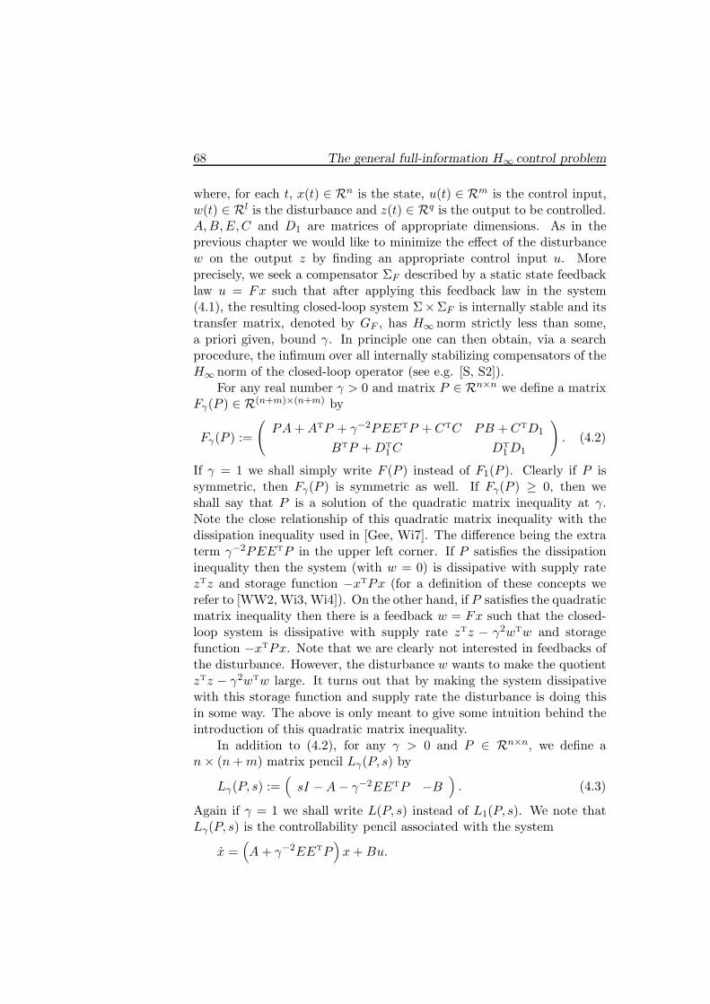
68 The general full-information H∞ control problem
where, for each t, x(t) ∈ Rn is the state, u(t) ∈ Rm is the control input,w(t) ∈ Rl is the disturbance and z(t) ∈ Rq is the output to be controlled.A,B,E,C and D1 are matrices of appropriate dimensions. As in theprevious chapter we would like to minimize the effect of the disturbancew on the output z by finding an appropriate control input u. Moreprecisely, we seek a compensator ΣF described by a static state feedbacklaw u = Fx such that after applying this feedback law in the system(4.1), the resulting closed-loop system Σ×ΣF is internally stable and itstransfer matrix, denoted by GF , has H∞ norm strictly less than some,a priori given, bound γ. In principle one can then obtain, via a searchprocedure, the infimum over all internally stabilizing compensators of theH∞ norm of the closed-loop operator (see e.g. [S, S2]).
For any real number γ > 0 and matrix P ∈ Rn×n we define a matrixFγ(P ) ∈ R(n+m)×(n+m) by
Fγ(P ) :=
(PA+ATP + γ−2PEETP + CTC PB +CTD1
BTP +DT1C DT
1D1
). (4.2)
If γ = 1 we shall simply write F (P ) instead of F1(P ). Clearly if P issymmetric, then Fγ(P ) is symmetric as well. If Fγ(P ) ≥ 0, then weshall say that P is a solution of the quadratic matrix inequality at γ.Note the close relationship of this quadratic matrix inequality with thedissipation inequality used in [Gee, Wi7]. The difference being the extraterm γ−2PEETP in the upper left corner. If P satisfies the dissipationinequality then the system (with w = 0) is dissipative with supply ratezTz and storage function −xTPx (for a definition of these concepts werefer to [WW2, Wi3, Wi4]). On the other hand, if P satisfies the quadraticmatrix inequality then there is a feedback w = Fx such that the closed-loop system is dissipative with supply rate zTz − γ2wTw and storagefunction −xTPx. Note that we are clearly not interested in feedbacks ofthe disturbance. However, the disturbance w wants to make the quotientzTz − γ2wTw large. It turns out that by making the system dissipativewith this storage function and supply rate the disturbance is doing thisin some way. The above is only meant to give some intuition behind theintroduction of this quadratic matrix inequality.
In addition to (4.2), for any γ > 0 and P ∈ Rn×n, we define an× (n+m) matrix pencil Lγ(P, s) by
Lγ(P, s) :=(sI −A− γ−2EETP −B
). (4.3)
Again if γ = 1 we shall write L(P, s) instead of L1(P, s). We note thatLγ(P, s) is the controllability pencil associated with the system
x =(A+ γ−2EETP
)x+Bu.

4.2 Problem formulation and main results 69
Gci will denote the transfer matrix of the system Σci := (A,B,C,D1)which is a subsystem of Σ as described by (4.1). We are now in theposition to formulate the main result of this chapter:
Theorem 4.1 : Consider the system (4.1). Let γ > 0. Assume that thesystem (A,B,C,D1) has no invariant zeros on the imaginary axis. Thenthe following three statements are equivalent:
(i) A static feedback law u = Fx exists such that after applying thiscompensator to the system (4.1) the resulting closed-loop system isinternally stable and the closed-loop operator GF has H∞ norm lessthan γ, i.e. ‖GF ‖∞ < γ.
(ii) (A,B) is stabilizable and for the system (4.1) a δ < γ exists suchthat for all w ∈ Ll2 there exists an u ∈ Lm2 such that xu,w ∈ Ln2 and‖zu,w‖2 ≤ δ‖w‖2.
(iii) A real symmetric solution P ≥ 0 to the quadratic matrix inequalityFγ(P ) ≥ 0 exists such that
rank Fγ(P ) = rankR(s)Gci (4.4)
and
rank
(Lγ(P, s)Fγ(P )
)= n+ rankR(s)Gci ∀s ∈ C0 ∪ C+. (4.5)
✷
Remarks :
(i) The implication (i) ⇒ (ii) is trivial. Hence we only need to prove(ii)⇒ (iii)⇒ (i). The first step will be done in the next section andin the section after that we shall complete the proof. We shall onlyprove this result for γ = 1, the general result can be easily obtainedby scaling.
(ii) The case that the assumption concerning the invariant zeros on theimaginary axis is not satisfied will be discussed in section 4.7. Theextension to the more general system (3.1), where D2 is arbitrary,will be discussed in section 4.6.

70 The general full-information H∞ control problem
Before embarking on a proof of this theorem we would like to point outhow the results from the previous chapter for D2 = 0 and D1 injectivecan be obtained from our theorem as a special case. First note that inthis case we have
rankR(s)Gci = rank D1 = m
Define
Rγ(P ) := PA+ATP + γ−2PEETP + CTC
− (PB + CTD1) (DT1D1)
−1 (BTP +DT1C) .
Furthermore, define a real (n+m)× (n+m) matrix by
S(P ) :=
(I − (PB + CTD1) (DT
1D1)−1
0 I
).
Then clearly we have
S(P )Fγ(P )S(P )T =
(Rγ(P ) 0
0 DT1D1
).
From this we can see that the conditions Fγ(P ) ≥ 0 and rankR(s)Fγ(P ) =m are equivalent to the single condition Rγ(P ) = 0. We now analyse thesecond rank condition appearing in our theorem. It is easy to verify thatfor all s ∈ C we have
I 0 B (DT
1D1)−1
0 I − (PB + CTD1) (DT1D1)
−1
0 0 I
(Lγ(P, s)Fγ(P )
)=
sI −A− γ−2EETP +B (DT
1D1)−1 (BTP +DT
1C) 0Rγ(P ) 0
BTP +DT1C DT
1D1
.
Consequently, if Rγ(P ) = 0, then for each s ∈ C the condition
rank
(Lγ(P, s)Fγ(P )
)= n+ rankR(s)Gci. (4.6)
is equivalent to
rank(sI −A− γ−2EETP +B (DT
1D1)−1 (BTP +DT
1C))= n

4.3 Solvability of the quadratic matrix inequality 71
and hence, since (4.6) should hold for all s ∈ C0 ∪ C+, we find that this isequivalent to the requirement that the matrix
A+ γ−2EETP −B (DT1D1)
−1 (BTP +DT1C)
is asymptotically stable. Theorem 3.1 for the case that D2 = 0 is thenobtained immediately.
4.3 Solvability of the quadratic matrixinequality
In this section we shall establish a proof of the implication (ii) ⇒ (iii)in theorem 4.1: assuming that the condition in part (ii) is satisfied weshall show that there is a solution of the quadratic matrix inequality thatsatisfies the two rank conditions. As announced just after theorem 4.1 weshall only prove this result for γ = 1. Therefore throughout this sectionwe assume that γ = 1.
Consider our system (4.1). For the special case that D1 is injective,we already have theorem 3.1 available. Our proof will use this result.
This time we do not make assumptions on the matrix D1. Choosebases in the state space, the input space and the output space as in ap-pendix A (where D is replaced by D1) and apply the preliminary feedbacku = F0x+ v where F0 is given by (A.1). We obtain the system
Σ :
{x = (A+BF0)x + Bv + Ew,
z = (C +D1F0)x + D1v(4.7)
After this transformation, in terms of our decomposition, we have theequations (A.5)–(A.7). We can consider our control system as the inter-connection of the subsystem Σ given by the equations (A.5) and (A.7)and the subsystem Σ0 given by (A.6). This interconnection is depicted inpicture (A.8). The idea we want to pursue is the following. We know con-dition (ii) of theorem 4.1 is still satisfied after the preliminary feedback,i.e. there exists a δ < 1 such that for all w ∈ Ll2 there exists a v ∈ Lm2such that
• ‖zv,w‖2 ≤ δ‖w‖2,• xv,w ∈ Ln2 .
(4.8)
Then, for a given w, let v be such that these conditions are satisfied.Define v1 as the first component of v and take x3 as the third component

72 The general full-information H∞ control problem
of xv,w. Interpret (v1, x3) as an input for the subsystem Σ defined by theequations (A.5) and (A.7). It then follows from (4.8) that
• ‖z1‖22 + ‖z2‖22 ≤ δ2‖w‖22,• x1 ∈ Ln2 .
Moreover note that the fictitious input x3 ∈ L2. Since w ∈ L2 was arbi-trary we note that Σ satisfies condition (ii) of theorem 4.1 with “inputs”(v1, x3), disturbance w and output (z1, z2). The crucial observation isnow that the direct-feedthrough matrix of Σ is injective (see lemma A.2).Thus we can apply theorem 3.1 to the system Σ. Before doing this weshould make sure that (A, (B11, A13)) is stabilizable and that Σci givenby (A.12) has no invariant zeros on the imaginary axis. It is easy to seethat if (A,B) is stabilizable, then (A, (B11, A13)) is also stabilizable. Fur-thermore if Σci = (A,B,C,D1) has no invariant zeros on the imaginaryaxis, then the same holds for Σci (see lemma A.3). Consequently, we mayapply theorem 3.1 to Σ and we obtain:
Corollary 4.2 : Consider the system (4.1). Assume that (A,B,C,D1)has no invariant zeros on the imaginary axis. Moreover, assume that part(ii) of theorem 4.1 is satisfied. Then a real symmetric solution P1 ≥ 0to the algebraic Riccati equation R(P1) = 0 exists, where R is defined by(A.17), such that Z(P1) is asymptoticaly stable, where Z is defined by(A.18). ✷
The basic idea pursued in section A.2 is that there is a one–one relationbetween solutions of the algebraic Riccati equation R(P1) = 0 and solu-tions of the quadratic matrix inequality Fγ(P ) ≥ 0 which satisfy the firstrank condition (4.4). This is formalized in theorem A.6. The implica-tion (ii) ⇒ (iii) is then obtained directly by combining corollary 4.2 withtheorem A.6.
4.4 Existence of state feedback laws
In this section we give a proof of the implication (iii) ⇒ (i) in theorem4.1. We shall first explain the idea of the proof. Again, we consider theparameters of our control system with respect to the bases of appendixA and after applying the preliminary feedback u = F0x + v where F0 isdefined by (A.1). In this way we obtain the system Σ defined by (4.7).Also, as in the previous section, we consider our control system as the

4.4 Existence of state feedback laws 73
interconnection of the subsystem Σ given by the equations (A.5) and (A.7)and the subsystem Σ0 given by (A.6). Suppose that the quadratic matrixinequality has a positive semi-definite solution at γ = 1 such that therank conditions (4.4) and (4.5) hold. Then, according to theorem A.6,the algebraic Riccati equation associated with the subsystem Σ (with“inputs” v1 and x3) has a positive semi-definite solution P1 such that thecorresponding matrix Z(P1), defined by (A.18), is asymptotically stable.Thus, by applying theorem 3.1 to the subsystem Σ, we find that the“feedback law”
v1 = −(DTD
)−1BT
11P1x1, (4.9)
x3 = − (CT23C23)
−1 (AT13P1 + CT
23C21) x1, (4.10)
applied to the system Σ yields an internally stable system and the closed-loop transfer matrix has H∞ norm smaller than 1. Now what we shall dois the following: we shall construct a state feedback law for the originalsystem (4.1) in such a way that in the subsystem Σ the equality (4.10)holds approximately and the equality (4.9) holds exactly. The closed-looptransfer matrix of the original system will then be approximately equalto that of the subsystem Σ and will therefore also have H∞ norm smallerthan 1.
In our proof an important role will be played by a result in the contextof the problem of almost disturbance decoupling as studied in [Tr] and[Wi5]. The results we need are recapitulated in section 2.6. We shall nowformulate and prove the converse of corollary 4.2:
Theorem 4.3 : Consider the system (4.1). Assume that (A,B,C,D1)has no invariant zeros on the imaginary axis. Assume that a real sym-metric solution P1 ≥ 0 to the algebraic Riccati equation R(P1) = 0 ex-ists, where R is defined by (A.17), such that Z(P1), defined by (A.18),is asymptotically stable. Then F ∈ Rm×n exists such that A + BF isasymptotically stable and such that after applying the state feedback lawu = Fx to Σ we have ‖GF ‖∞ < 1. ✷
Proof : Clearly it is sufficient to prove the existence of such state feed-back law v = Fx for the system (4.7). Let this system be decomposedaccording to (A.5)–(A.7). Choose
v1 = −(DTD
)−1BT
11P1x1

74 The general full-information H∞ control problem
and introduce a new state variable q3 by
q3 := x3 + (CT23C23)
−1 (AT13P1 + CT
23C21) x1
Then the equations (A.5)–(A.7) can be rewritten as
x1 = A11x1 +A13q3 + E1w, (4.11)
(x2
q3
)=
(A22 A23
A32 A33
)(x2
q3
)+
(B22
B32
)v2 +
(A21
A31
)x1 +
(E2
E3
)w, (4.12)
(z1
z2
)=
(C1
C2
)x1 +
(0C23
)q3. (4.13)
Here we used the following definitions:
A11 := A11 −A13(CT23C23)−1(AT
13P1 + CT23C21)
−B11(DTD)−1BT11P1,
A21 := A21 −A23(CT23C23)−1(AT
13P1 + CT23C21)
−B21(DTD)−1BT11P1,
A31 := A31 −A33(CT23C23)−1(AT
13P1 + CT23C21)
−B31(DTD)−1BT11P1
+(CT23C23)−1(AT
13P1 + CT23C21)A11,
A33 := A33 + (CT23C23)−1(AT
13P1 + CT23C21)A13,
C1 := −D(DTD)−1BT11P1,
C2 := C21 − C23(CT23C23)−1(AT
13P1 + CT23C21),
E3 := E3 + (CT23C23)−1(AT
13P1 + CT23C21)E1.
By corollary (A.8), we know that A11 is asymptotically stable. Accordingto theorem 3.1, if in the subsystem formed by the equations (4.11) and(4.13) we have q3 = 0, then its transfer matrix from w to z has H∞ normsmaller than 1. Moreover, by corollary (A.8), we know that A11 is asymp-totically stable. Hence, there exist M > 0 and ρ > 0 such that for all wand q3 in L2 we have
‖z‖2 < (1− ρ)‖w‖2 +M‖q3‖2 (4.14)
Also, since A11 is asymptotically stable, M1,M2 > 0 exist such that forall w and q3 in L2 we have
‖x1‖2 < M1‖w‖2 +M2‖q3‖2. (4.15)

4.4 Existence of state feedback laws 75
We claim that the following system is strongly controllable:[(A22 A23
A32 A33
),
(B22
B32
),(0 I
), 0
](4.16)
This can be seen by the following transformation:I 0 00 I A33 − A33
0 0 I
sI −A22 −A23 −B22
−A32 sI −A33 −B32
0 I 0
=
sI −A22 −A23 −B22
−A32 sI − A33 −B32
0 I 0
.
Since the first matrix on the left is unimodular and the second matrixhas full row rank for all s ∈ C (combine lemmas 2.8 and A.2), the matrixon the right has full row rank for all s ∈ C. Hence the system (4.16) isstrongly controllable by lemma 2.8.
Consider now the almost disturbance decoupling problem for the sys-tem (4.12) with output q3 and “disturbance” (x1, w). According to lemma2.17 the strong controllability of (4.16) implies that there exists a feedbacklaw
v2 = F1
(x2
q3
)
such that in (4.12) we have
‖q3‖2 <ρ
2(M +M1M + ρM2)
−1 {‖w‖2 + ‖x1‖2} (4.17)
for all w and x1 in L2, and such that the matrix
A :=
(A22 A23
A32 A33
)+
(B22
B32
)F1
is asymptotically stable. Combining (4.14), (4.15) and (4.17) gives us
‖z‖2 <(1− ρ
2
)‖w‖2
for all w in L2. Summarizing, we have shown that if in our original system(4.7) we apply the state feedback law
v1 = −(DTD
)−1BT
11P1x1
v2 = F1
(x2
x3 + (CT23C23)
−1 (AT13P1 + CT
23C21) x1
),
(4.18)

76 The general full-information H∞ control problem
then for all w ∈ Ll2 we have ‖z‖2 < δ‖w‖2 with δ < 1. Thus, theH∞ normof the resulting closed-loop transfer matrix is smaller than 1.It remains to be shown that the closed-loop system is internally stable.We know that
‖(sI − A11
)−1A13‖∞ ≤M2 (4.19)
‖(0 I
) (sI − A
)−1(A21
A31
)‖∞ ≤ ρ
2(M +M1M + ρM2)
−1
≤ 12M2
(4.20)
The closed-loop state matrix resulting from the feedback (4.18) is givenby
Acl :=
A11
(0 A13
)(A21
A31
)A
Assume that (xT, yT, zT)T is an eigenvalue of Acl with eigenvalue λ withRe λ ≥ 0. It can be seen that
x =(λI − A11
)−1A13z, (4.21)
z =(0 I
) (λI − A
)−1(A21
A31
)x. (4.22)
(Note that the inverses exist due to the fact that A11 and A are stablematrices.) Combining (4.19) and (4.21) we find ‖x‖ ≤ M2‖z‖ and com-bining (4.20) and (4.22) yields ‖x‖ ≥ 2M2‖z‖. Hence x = z = 0. Thiswould however imply that ( yT 0 )T is an unstable eigenvector of A.Since A is asymptotically stable this yields a contradiction. This provesthat the closed-loop system is internally stable.
Again using the one–one relation between solutions of the Riccati equationand solutions of the quadratic matrix inequality as given in theorem A.6,the implication (iii) ⇒ (i) in theorem 4.1 is now obtained by combiningtheorem A.6 and theorem 4.3.
Remarks : In the regular case (i.e. D1 injective) it is quite easy togive an explicit expression for a suitable state feedback law. This was

4.5 The design of a suitable compensator 77
done in theorem 3.1. In the singular case (i.e. D1 is not injective) asuitable state feedback law is given by u = F0x+ v. Here, F0 is given by(A.1) and v = ( vT
1 vT2 )T is given by (4.18). The matrix P1 is obtained
by solving the quadratic matrix inequality or, equivalently, by solvingthe reduced order Riccati equation R(P1) = 0 where R is defined by(A.17). The matrix F1 is a “state feedback” for the strongly controllableauxiliary system (4.12). This state feedback achieves almost disturbancedecoupling between the “disturbance” (x1, w) and the “output” q3. Therequired accuracy of decoupling is expressed by (4.17). A conceptualalgorithm to construct F1 is given in section 4.5. In this section wealso discuss the numerical reliability of several algorithms available in theliterature.
4.5 The design of a suitable compensator
Several algorithms are available in the literature for the construction of asuitable compensator for singular H∞ control problems. The best-knownalgorithm is a small perturbation of the system parameters such thatthe perturbed system becomes regular. We can then apply the results ofthe previous chapter where a suitable controller is given explicitly. Thismethod is outlined in subsection 4.7.2.
An alternative approach is to use the steps outlined in this chapter.In other words, bring the system in the form of the basis of appendixA. Then a suitable controller is given by (4.18) where F1 should be suchthat (4.17) is satisfied. Hence the problem is reduced to finding a statefeedback for the strongly controllable system defined by the quadruple in(4.16) such that the closed-loop H∞ norm is less than:
δ :=ρ
2(M +M1M + ρM2)
−1
∥∥∥∥∥(A21 E2
A31 E3
)∥∥∥∥∥where all matrices are as defined in the previous section. We shall de-scribe a method which is an adapted version of the one given in [Tr]. Analternative method is described in [OSS1].
We denote the first three matrices of the quadruple in (4.16) by A,B and C respectively.
(i) We construct a new basis for the state space. We shall construct itby induction. Choose 0 �= x1 ∈ ker C ∩ im B and, if such x1 exists,choose v1 such that Bv1 = x1. If x1 does not exist then set i = 0and Si = {0} and go to item (ii).

78 The general full-information H∞ control problem
Assume that {x1, . . . , xi} and {v1, . . . , vi} are given. Denote bySi the linear span of {x1, . . . , xi}. If (Axi + im B) ∩ ker C ⊂ Siand im B ∩ ker C ⊂ Si then go to step (ii). Otherwise, if (Axi +im B)∩ ker C �⊂ Si then choose v such that Axi+ Bv ∈ ker C andAxi+Bv �∈ Si. Set xi+1 = Axi+Bv and vi+1 = v. If (Axi+ im B)∩ker C ⊂ Si, then choose v such that Bv ∈ ker C and Bv �∈ Si. Setxi+1 = Bv and vi+1 = v. Set i := i + 1 and repeat this paragraphagain.
(ii) DefineR∗a( ker C) = Si. Define a linear mapping F such that Fxj =
vj , j = 1, . . . , i and extend it arbitrarily to the whole state space.In [Tr] it has been shown that AR∗
a( ker C)+ im B = T (Σht) = Rn.Therefore we can extend the basis of Si, {x1, . . . , xi} to a basis ofRn which can be written as
Bv1, AF Bv1, . . . , Ar1F Bv1,
Bv2, AF Bv2, . . . , Ar2F Bv2,
......
...Bvi, AF Bvi, . . . , Ari
F Bvi,
Bvi+1, . . . , Bvk,
where AF = A + BF and where we may have to extend our set{v1, . . . , vi} with some vectors vj, j = i+1, . . . , k in order to obtaina basis of Rn. Moreover, for j = 1, . . . , i we should have
Bvj , AF Bvj , . . . , Arj−1F Bvj ∈ ker C.
We define rj = 0 for j = i+ 1, . . . , k.
(iii) We define the following sequence of vectors. For j = 1, . . . , k wedefine:
xj,1(n) :=(I + 1
nAF
)−1Bvj
xj,2(n) :=(I + 1
nAF
)−1AFxj,1(n)
......
...
xj,rj+1(n) :=(I + 1
nAF
)−1AFxj,rj(n)
It is easily shown that xj,h(n)→ Ah−1F Bvj as n→∞ for j = 1, . . . , k
and h = 1, . . . , rj+1. Therefore, for n sufficiently large, the vectors
{xj,h(n), j = 1, . . . , k; h = 1, . . . , rj + 1}

4.5 The design of a suitable compensator 79
are linearly independent and hence form a basis of Rn again. LetN be such that for all n > N these vectors indeed form a basis.
(iv) For all n > N define a linear mapping Fn by
Fnxj,1(n) := −nvjFnxj,2(n) := −n2vj
......
Fnxj,rj+1(n) := −nrj+1vj
for j = 1, . . . , k. This determines Fn uniquely. Define Fn := F+Fn.It is shown in [Tr] that the spectrum of A + BFn is the set {−n}.Moreover, we have
limn→∞ ‖Ce
(A+BFn)t ‖1 = 0
Choose n such that the impulse response has L1 norm smaller thanδ.
We would like to conclude this section by comparing the three methodsmentioned in this section. Several numerical problems arise:
(i) In order to transform the system in the bases of appendix A weneed the subspace T (Σci). The construction of this subspace asgiven in lemma 2.5 depends strongly on the determination of kernelsand images of matrices. However, a rank evaluation is needed todetermine, e.g. the kernel, and this is known to be a numericallyill-posed problem. To determine this subspace we can also use thealgorithm as described in [SS]. This has the same problem but thisalgorithm has been thoroughly tested via examples and seems towork well.
(ii) The method described in this section and also the method describedin subsection 4.7.2 involves a parameter (ε and 1/n respectively)which goes to infinity. This also results in numerical problems.
Fortunately there is an easy and numerically reliable test whether theresulting feedback is stabilizing and satisfies the H∞ norm bound for theclosed-loop system. A good algorithm to calculate the H∞ norm can befound in [BBK, BS]. In other words, we can check whether the numericalproblems resulted in a bad design.
The algorithm in [OSS1, OSS2] also involves rank evaluations. How-ever, by using the infinite zero structure and especially the different

80 The general full-information H∞ control problem
timescales of eigenvalues that go to infinity, this algorithm results in feed-backs with lower gain to achieve the same level of disturbance decoupling.Ozcetin et al.’s work shows that combining the results in this book on thesingular H∞ control problem with their algorithm yielded better results(i.e. lower feedback gain) in all the examples they tried when comparedto the often proposed technique of subsection 4.7.2.
4.6 A direct-feedthrough matrix from disturbance
to output
In this section we shall show how to handle the state feedback case forthe more general system
Σ :
{x = Ax + Bu + Ew,
z = Cx + D1u + D2w.(4.23)
(i.e. we allow for D2 �= 0). We shall use a technique from [Gl6] to reducethis problem to the problem studied in section 4.2. Throughout thissection we shall assume that γ = 1. The more general result can beeasily derived by scaling. There is one notable difference between theregular case and the singular case if the extra direct-feedthrough matrixis present. In the regular case conditions (i) and (ii) of theorem 3.1 areequivalent. This is not true in the singular case. An easy counter exampleis the following:
Example 4.4 : Let the following system be given:
Σ :
{x = u,
z = x + 100w.
After applying an arbitrary static feedback of the form u = f1x+ f2w theclosed-loop transfer matrix will be given by
gf (s) =f2
s− f1+ 100.
Clearly ‖gf‖∞ ≥ 100. However, if we set u = −100w, then z = 0 for allw which are differentiable and satisfy w(0)=0 (if w is not differentiableor if w(0) �= 0, then we can approximate w arbitrarily by a differentiablefunction w1 which satisfies w1(0) = 0). This implies that condition (ii)of theorem 3.1 is satisfied but on the other hand condition (i) of theorem3.1 is certainly not satisfied. This yields the desired contradiction. ✷

4.6 An extra direct-feedthrough matrix 81
In general the controllers we would need in the case that condition (ii) issatisfied while condition (i) is not satisfied will be non-proper, i.e. they willinclude differentiations of the disturbance. Since this is very undesirablewe shall focus all our attention on controllers of the form (2.4). We shallrestrict ourselves to the case of state feedback, i.e. y = x. The result forthe full-information case, i.e. y = (x,w), can be obtained in a similar way.
It is easily seen that when there exists a dynamic controller of theform (2.4) where y = x which makes the H∞ norm less than 1 then‖D2‖ < 1. We therefore assume that ‖D2‖ < 1. We define the followingmatrices
AD := A+ E (I −DT2D2)
−1DT
2C,
BD := B + E (I −DT2D2)
−1DT2D1,
ED := −E (I −DT2D2)
−1/2 ,
CD := (I −D2DT2 )
−1/2 C,
D1,D := (I −D2DT2 )
−1/2D1.
Using these matrices we define the following system:
ΣD :
{xD = ADxD + BDuD + EDwD,
zD = CDxD + D1,DuD.(4.24)
We have the following lemma connecting ΣD and Σ:
Lemma 4.5 : Let ΣF be a dynamic controller of the form (2.4). Con-sider the following two systems:
Σ
ΣF
❄
✛
✻
✛
y = x
z w
u
ΣD
ΣF
❄
✛
✻
✛
yD = xD
zD wD
uD(4.25)
The system on the left is the interconnection of Σ described by (4.23) andΣF described by (2.4). The system on the right is the interconnectionof ΣD described by (4.24) and the same feedback compensator ΣF . Thefollowing two conditions are equivalent
(i) The system on the left is internally stable and the closed-loop trans-fer matrix from w to z has H∞ norm less than 1.
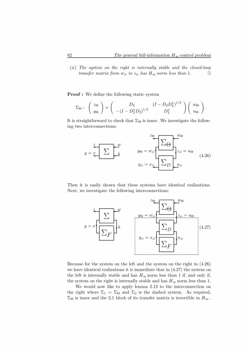
82 The general full-information H∞ control problem
(ii) The system on the right is internally stable and the closed-looptransfer matrix from wD to zD has H∞ norm less than 1. ✷
Proof : We define the following static system
ΣΘ :
(zΘ
yΘ
)=
(D2 (I −D2D
T2 )
1/2
− (I −DT2D2)
1/2 DT2
)(wΘ
uΘ
).
It is straightforward to check that ΣΘ is inner. We investigate the follow-ing two interconnections:
Σ
ΣD
ΣΘ
✛y = x
✛
✛u
✛
✛yD = xD
✛
✛uD
✛
❄✻
z w
zΘ wΘ
yΘ = wD zD = uΘ(4.26)
Then it is easily shown that these systems have identical realizations.Next, we investigate the following interconnections:
Σ
ΣDΣF
ΣF
ΣΘ
❄
✛
✻
✛
❄
✛
✻
✛
❄✻
y = x
z w
u
zΘ
yD = xD uD
wΘ
yΘ = wD zD = uΘ
(4.27)
Because for the system on the left and the system on the right in (4.26)we have identical realizations it is immediate that in (4.27) the system onthe left is internally stable and has H∞ norm less than 1 if, and only if,the system on the right is internally stable and has H∞ norm less than 1.
We would now like to apply lemma 2.12 to the interconnection onthe right where Σ1 = ΣΘ and Σ2 is the dashed system. As required,ΣΘ is inner and the 2,1 block of its transfer matrix is invertible in H∞ .

4.6 An extra direct-feedthrough matrix 83
However, the 2,2 block of its transfer matrix, G22, is not strictly proper.On the other hand, if one checks the proof of lemma 2.12 it is easily seenthat the requirement that G22 is strictly proper is only needed to showthat I−G22G2 is invertible as a rational matrix, where G2 is the transfermatrix of the dashed system. It is easy to check that I−G22G2 evaluatedat infinity is equal to I −DT
2D2. Hence, since I −DT2D2 is invertible, the
rational matrix I − G22G2 is invertible. This implies that the result oflemma 2.12 is still valid. Therefore in (4.27) the system on the right isinternally stable and has H∞ norm less than 1 if, and only if, the dashedsystem is internally stable and has H∞ norm less than 1.
Combining, we find that in (4.27) the system on the left is internallystable and has H∞ norm less than 1 if, and only if, the dashed system isinternally stable and has H∞ norm less than 1. By noting that the systemon the left in (4.27) is equal to the system on the left in (4.25) and thedashed system in (4.27) is equal to the system on the right in (4.25) thiscompletes the proof.
We can also derive the following result:
Lemma 4.6 : Assume that the system Σ and the system ΣD, describedby (4.23) and (4.24), respectively, are given. The invariant zeros of(A,B,C,D1) are equal to the invariant zeros of (AD, BD, CD,D1,D). ✷
Proof : We have the following relationship between the system matricesof the systems (A,B,C,D1) and (AD, BD, CD,D1,D) respectively:(
I EDT2 (I −D2D
T2 )
−1/2
0 (I −D2DT2 )
1/2
)(sI −AD −BD
CD D1,D
)=
(sI −A −BC D1
).
Since the first matrix on the left is unimodular, the above equality im-mediately gives the desired result.
We shall now state and prove the results for the more general system(4.23). The following theorem generalizes theorem 3.2.
Theorem 4.7 : Let the system Σ described by (4.23) be given. Assumethat (A,B,C,D1) has no invariant zeros on the imaginary axis. Thenthe following three statements are equivalent:

84 The general full-information H∞ control problem
(i) A compensator ΣF described by the static state feedback law u = Fxexists such that the closed-loop system Σ × ΣF is internally stableand has H∞ norm less than 1.
(ii) A compensator ΣF of the form (2.4) with y=x exists such that theclosed-loop system Σ × ΣF is internally stable and has H∞ normless than 1.
(iii) We have ‖D2‖ < 1 and ΣD defined by (4.24) satisfies condition (iii)of theorem 4.1 with γ = 1. ✷
Proof : The implication (i) ⇒ (ii) is trivial.(ii) ⇒ (iii): Note that if there is a dynamic state feedback which
makes the H∞ norm less than 1, then ‖D2‖ < 1. By lemma 4.5 if thereis an internally stabilizing controller ΣF which makes the H∞ norm lessthan 1, then the same controller is internally stabilizing for the systemΣD defined by (4.24) and this controller also makes the H∞ norm of theclosed-loop system ΣD × ΣF less than 1. By lemma 4.6 ΣD satisfiesthe assumptions of theorem 4.1 and we already know that ΣD satisfiescondition (ii) of theorem 4.1. Therefore condition (iii) of theorem 4.1 issatisfied for the system ΣD.
(iii) ⇒ (i): By lemma 4.6 the system ΣD satisfies the assumptionsof theorem 4.1 and moreover condition (iii) of theorem 4.1 is satisfied.Therefore, the system ΣD satisfies condition (i) of theorem 4.1. Thisimplies that for the system ΣD there is an internally stabilizing staticstate feedback which makes the closed-loop H∞ norm less than 1. Finallyby lemma 4.5 this state feedback satisfies condition (i) of theorem 4.7 forthe system Σ.
4.7 Invariant zeros on the imaginary axis
In this section we shall discuss two methods which can be used to solvethe H∞ problem with zeros on the imaginary axis. A method we shallnot discuss and which is given in [S3] will probably lead to much moreelegant conditions but these conditions are too complex to explain here indetail (some discussions on this alternative method are given in subsection12.2.1).

4.7 Invariant zeros on the imaginary axis 85
4.7.1 Frequency-domain loop shifting
The basic method (see [Kh2, Li3, Sa]) here is based on applying a trans-formation in the frequency-domain. This method is applicable for thefull-information feedback case. On the other hand, for the state feedbackcase we have, after transformation, a problem with measurement feed-back which we can only solve using techniques which will be given in thenext chapter. Therefore we assume that y = (x,w).
For all ε > 0 we define the following transformation:
G(s) −→ G(s) := G
(ε+ s1 + εs
)
and instead of minimizing the H∞ norm of a system described by thetransfer matrix G we minimize the H∞ norm of a system described bythe transfer matrix G. If I − εA is invertible a state space realization ofG is given by:
Σ(ε) :
x = Ax + Bu + Ew,
y = C1x + D11u + D12w,
z = C2x + D21u + D22w,
(4.28)
where
A := (A− εI)(I − εA)−1,
B := (1− ε2)(I − εA)−1B,
E := (1− ε2)(I − εA)−1E,
C1 :=
((I − εA)−1
0
),
C2 := C(I − εA)−1,
D11 :=
(ε(I − εA)−1B
0
),
D12 :=
(ε(I − εA)−1E
I
),
D21 := D1 + εC(I − εA)−1B,
D22 := D2 + εC(I − εA)−1E.
Assume that a compensator ΣF described by u = F1x + F2w for Σ(ε)exists such that the closed-loop system is internally stable, the closed-loop transfer matrix Gcl has H∞ norm less than 1 and, moreover, the

86 The general full-information H∞ control problem
matrix I − εBF1 is invertible (the latter we can always achieve by anarbitrarily small perturbation). We define
F :=(F1(I + εBF1) F2
)(I − εA −ε(E −BF2)0 I
). (4.29)
The feedback u = F y applied to the same system Σ(ε) but with y insteadof y = (x,w) yields the same closed-loop system and is hence internallystabilizing and the closed-loop transfer matrix is Gcl.
If we apply the feedback ΣF described by u = Fy to our originalsystem, then the closed-loop system ΣF × Σ, with transfer matrix Gcl,is related to the closed-loop system Σ(ε)× ΣF , with transfer matrix Gcl,via the above transformation, i.e.
Gcl(s) = Gcl
(ε+ s1 + εs
).
Moreover, it can be shown that the state matrix of the closed-loop systemΣ × ΣF has all its eigenvalues inside a circle D which is symmetric withrespect to the real axis and lies in the left half plane between −ε and −1/ε.Hence the closed-loop system is certainly internally stable. Denote theset of all s ∈ C outside that circle by D+. We have
1 > ‖GF ‖∞ = sups∈C+
‖GF (s)‖ = sups∈D+
‖GF (s)‖
≥ sups∈C+
‖GF (s)‖ = ‖GF ‖∞.
Hence ΣF makes the H∞ norm of the closed-loop transfer matrix GF
strictly less than 1.On the other hand, if, for the system Σ, there is a stabilizing static
compensator ΣF with y = (x,w) which makes the H∞ norm of the closed-loop system strictly less than 1 then it can be shown that ε1 > 0 existssuch that for all 0 < ε ≤ ε1 the transformed system Σ(ε) with the samecompensator ΣF but with measurement y is internally stable and theH∞ norm of the closed-loop system is strictly less than 1.
Now for all but finitely many ε > 0 the system Σ(ε), described by(4.28) is such that (A, B, C2, D21) has no invariant zeros on the imagi-nary axis. Therefore to check if for Σ(ε) there is an internally stabilizingfeedback which makes the H∞ norm of the closed-loop system less than1 we can use the results of the previous section.
We can formalize the above intuition in the following theorem. Weshall not formally prove this theorem.
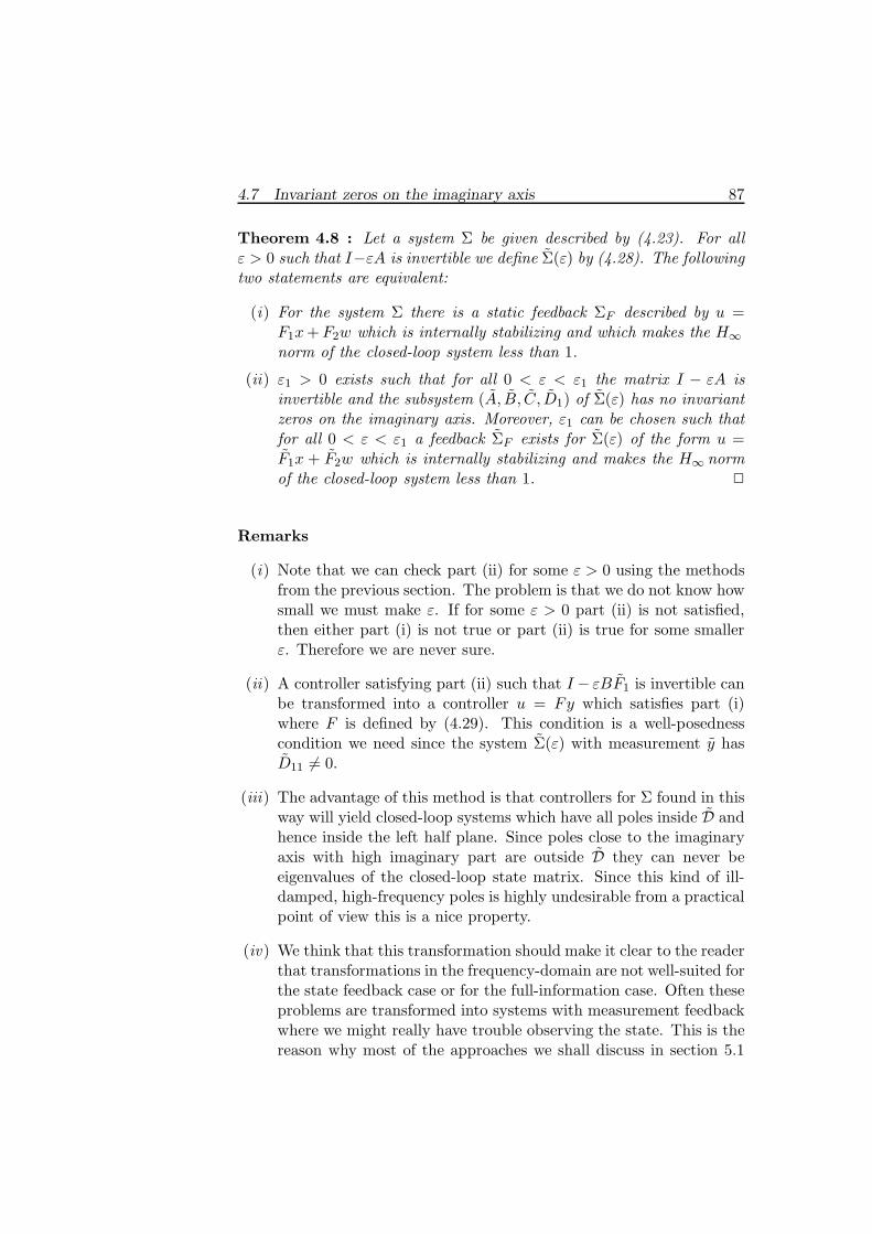
4.7 Invariant zeros on the imaginary axis 87
Theorem 4.8 : Let a system Σ be given described by (4.23). For allε > 0 such that I−εA is invertible we define Σ(ε) by (4.28). The followingtwo statements are equivalent:
(i) For the system Σ there is a static feedback ΣF described by u =F1x+F2w which is internally stabilizing and which makes the H∞norm of the closed-loop system less than 1.
(ii) ε1 > 0 exists such that for all 0 < ε < ε1 the matrix I − εA isinvertible and the subsystem (A, B, C, D1) of Σ(ε) has no invariantzeros on the imaginary axis. Moreover, ε1 can be chosen such thatfor all 0 < ε < ε1 a feedback ΣF exists for Σ(ε) of the form u =F1x + F2w which is internally stabilizing and makes the H∞ normof the closed-loop system less than 1. ✷
Remarks
(i) Note that we can check part (ii) for some ε > 0 using the methodsfrom the previous section. The problem is that we do not know howsmall we must make ε. If for some ε > 0 part (ii) is not satisfied,then either part (i) is not true or part (ii) is true for some smallerε. Therefore we are never sure.
(ii) A controller satisfying part (ii) such that I − εBF1 is invertible canbe transformed into a controller u = Fy which satisfies part (i)where F is defined by (4.29). This condition is a well-posednesscondition we need since the system Σ(ε) with measurement y hasD11 �= 0.
(iii) The advantage of this method is that controllers for Σ found in thisway will yield closed-loop systems which have all poles inside D andhence inside the left half plane. Since poles close to the imaginaryaxis with high imaginary part are outside D they can never beeigenvalues of the closed-loop state matrix. Since this kind of ill-damped, high-frequency poles is highly undesirable from a practicalpoint of view this is a nice property.
(iv) We think that this transformation should make it clear to the readerthat transformations in the frequency-domain are not well-suited forthe state feedback case or for the full-information case. Often theseproblems are transformed into systems with measurement feedbackwhere we might really have trouble observing the state. This is thereason why most of the approaches we shall discuss in section 5.1

88 The general full-information H∞ control problem
for the H∞ control problem with measurement feedback are oftennot very suitable to treat the special cases of state feedback andfull-information feedback.
4.7.2 Cheap control
In this subsection we shall briefly describe how the method used in [Kh3,Kh2, Pe3, Pe5, ZK2] still gives necessary and sufficient conditions for theexistence of internally stabilizing controllers which make the H∞ norm ofthe closed-loop system less than 1 even when we have invariant zeros onthe imaginary axis. This subsection is worked out in more detail in [St].
We assume that we have a system Σ of the form (4.23). For eachε > 0 we define the following system:
Σ(ε) :
{x = Ax + Bu + Ew,
z = Cx + D1u + D2w,(4.30)
where
C =
C
εI
0
, D1 =
D1
0εI
, D2 =
D2
00
.
The structure of the perturbations on the matrices is such that it is easyto show that any controller ΣF of the form (2.4) with y = x has theproperty that ΣF is internally stabilizing when applied to Σ if, and onlyif, the same controller ΣF is internally stabilizing when applied to Σ(ε)(for y = (x,w), the same is true).
Let ΣF be internally stabilizing when applied to Σ. Denote the closed-loop operator by GF . Moreover denote the closed-loop operator when thecontroller is applied to Σ(ε) by GF (ε). Then we have
‖GF ‖∞ ≤ ‖GF (ε1)‖∞ ≤ ‖GF (ε2)‖∞
for all 0 ≤ ε1 ≤ ε2. Hence if we have an internally stabilizing controllerwhich makes the H∞ norm of the closed-loop system less than 1 whenapplied to the system GF (ε), then the same controller is internally stabi-lizing and makes the H∞ norm of the closed-loop system less than 1 whenapplied to the original system. Thus we can obtain the following result:
Theorem 4.9 : Let a system Σ be given by (4.23). For all ε > 0 defineΣ(ε) by (4.28). The following two statements are equivalent:
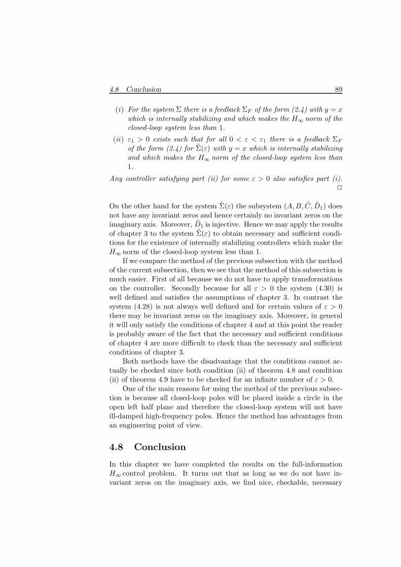
4.8 Conclusion 89
(i) For the system Σ there is a feedback ΣF of the form (2.4) with y = xwhich is internally stabilizing and which makes the H∞ norm of theclosed-loop system less than 1.
(ii) ε1 > 0 exists such that for all 0 < ε < ε1 there is a feedback ΣF
of the form (2.4) for Σ(ε) with y = x which is internally stabilizingand which makes the H∞ norm of the closed-loop system less than1.
Any controller satisfying part (ii) for some ε > 0 also satisfies part (i).✷
On the other hand for the system Σ(ε) the subsystem (A,B, C, D1) doesnot have any invariant zeros and hence certainly no invariant zeros on theimaginary axis. Moreover, D1 is injective. Hence we may apply the resultsof chapter 3 to the system Σ(ε) to obtain necessary and sufficient condi-tions for the existence of internally stabilizing controllers which make theH∞ norm of the closed-loop system less than 1.
If we compare the method of the previous subsection with the methodof the current subsection, then we see that the method of this subsection ismuch easier. First of all because we do not have to apply transformationson the controller. Secondly because for all ε > 0 the system (4.30) iswell defined and satisfies the assumptions of chapter 3. In contrast thesystem (4.28) is not always well defined and for certain values of ε > 0there may be invariant zeros on the imaginary axis. Moreover, in generalit will only satisfy the conditions of chapter 4 and at this point the readeris probably aware of the fact that the necessary and sufficient conditionsof chapter 4 are more difficult to check than the necessary and sufficientconditions of chapter 3.
Both methods have the disadvantage that the conditions cannot ac-tually be checked since both condition (ii) of theorem 4.8 and condition(ii) of theorem 4.9 have to be checked for an infinite number of ε > 0.
One of the main reasons for using the method of the previous subsec-tion is because all closed-loop poles will be placed inside a circle in theopen left half plane and therefore the closed-loop system will not haveill-damped high-frequency poles. Hence the method has advantages froman engineering point of view.
4.8 Conclusion
In this chapter we have completed the results on the full-informationH∞ control problem. It turns out that as long as we do not have in-variant zeros on the imaginary axis, we find nice, checkable, necessary

90 The general full-information H∞ control problem
and sufficient conditions under which there exist an internally stabilizingcontroller which makes the H∞ norm of the closed-loop system less thansome, a priori given, bound γ. In the case that we have a regular pro-blem we have one Riccati equation and, if one exists, an explicit formulafor one suitable controller. On the other hand, for the singular problemwe have a quadratic matrix inequality and a couple of rank conditions.Using a state space decomposition, the latter conditions can be shown tobe equivalent to a reduced order Riccati equation (see appendix A). Aproblem is that we do not have an explicit formula for the desired con-troller and there may be numerical problems when trying to find such acontroller.
When there are invariant zeros on the imaginary axis the methods ofsection 4.7 can be used. However, these methods are not really satisfac-tory and one would have to investigate the technique used in [S3] betterto obtain nicer conditions for the general case (the conditions we have inmind are suggested in subsection 12.2.1).

Chapter 5
The H∞ control problem withmeasurement feedback
5.1 Introduction
In the previous two chapters we investigated two special cases of theH∞ control problem with measurement feedback, namely y = x and y =(x,w). In this chapter we shall investigate the more general system (2.1).
Around 1984 practically all the work on H∞ control theory withmeasurement feedback was done with a mixture of time-domain andfrequency-domain techniques (see [Do3, Fr2, Gl, Gl6]). The main draw-back of these methods was that it yielded high order controllers. In[Li, Li2] it was shown that the order of the controller could be reducedconsiderably: it was proven that for the one block H∞ control problem(the matrices D12 and D21 appearing in (2.1) are both square matrices)and for the two block H∞ control problem (either the matrix D12 or thematrix D21 in (2.1) is a square matrix) there are always “suitable” con-trollers with an order no greater than the order of the plant.
During the last few years the H∞ control problem with measurementfeedback was investigated via several new methods:
• The interpolation approach. In fact, the interpolation approachalready has quite a history and several authors have worked on thisproblem (see e.g. [Gr, Kh, Li3, Za2]). However, it can only treatthe special case of a one-block H∞ control problem. One shouldnote that the classic interpolation techniques were used for discretetime systems. At first the continuous time case was treated via afrequency-domain transformation to the discrete time case (a linearfractional transformation as given in [Gen, appendix 1]).
• The time-domain approach (see [Do5, Kh3, Kh4, Pe, Ta]). This
91

92 H∞ control with measurement feedback
method was the first to suggest the use of Riccati equations inH∞ control, which was an important breakthrough. The detailedformulations of the results obtained via this method will be givenin this chapter.
• The polynomial approach (see [Bo, Kw, Kw2]). This methodstarts with a polynomial left (or right) coprime factorization of thetransfer matrix of the system. Then it is shown that a controllerwhich minimizes the H∞ norm of the closed-loop system is a so-called equalizing solution of a certain minimization problem. Con-ditions for obtaining an internally stabilizing controller which min-imizes the H∞ norm are then given in terms of diophantine equa-tions. The current research in this area is to investigate the relationbetween these diophantine equations and the conditions found inother methods.
• The J-spectral factorization approach (see [Gr2, HSK, Ki]).This method is strongly based on the classic frequency-domain ap-proach. The conditions for the existence of an internally stabilizingcontroller which makes the H∞ norm of the closed-loop system lessthan some, a priori given, bound are given in terms of a rational ma-trix which should have a so-called J-spectral factorization. Whethersuch a factorization exists can be checked via the solvability of cer-tain algebraic Riccati equations.
All of these methods show that if suitable controllers exist, then a suitablecontroller can be found of the same complexity as the original plant. Asecond feature that all of these methods have in common is a number ofbasic assumptions they all have to make. The assumptions are twofold.Firstly two direct-feedthrough matrices should be injective and surjective,respectively. Secondly, two given subsystems should not have invariantzeros on the imaginary axis. These assumptions exclude, for instance, thespecial cases of state feedback and full-information feedback.
A special feature of the time-domain approach we are using through-out this book is that it first solves the full-information feedback case aswe did in the previous chapters and then uses these results to obtain thegeneral result.
Under the basic assumptions mentioned above and using the time-domain approach, the necessary and sufficient conditions for the existenceof internally stabilizing controllers which make theH∞ norm of the closed-loop system less than some, a priori given, bound γ are the following: twogiven Riccati equations should have positive semi-definite solutions andthe product of these two matrices should have spectral radius less than

5.1 Introduction 93
γ2. These two Riccati equations are not coupled and in fact one of themis the same as the Riccati equation from chapter 3. The other Riccatiequation is dual to the first one and is related to the problem of stateestimation. The coupling condition that the product of the solutions ofthese Riccati equations should have spectral radius less than γ2 is veryhard to explain intuitively. It is a kind of test whether state estimationand state feedback combined in some way yield the desired result: aninternally stabilizing feedback which makes the H∞ norm less than γ.The most general result under these assumptions is stated without proofin [Gl3].
In the literature two methods have been proposed to solve theH∞ pro-blem without assumptions on the direct-feedthrough matrices and with-out assumptions on the invariant zeros. For the special case of full-information feedback, these methods are discussed in section 4.7. Usingthe first method discussed in subsection 4.7.1, which applies a transforma-tion in the complex plane combined with the results in [Do5, Kh3, Pe, Ta],we still have to make assumptions: two given subsystems should be leftand right invertible respectively. The second method combined with themethods of the latter papers can tackle the most general case. Thesemethods, however, have the drawback that the conditions are in terms ofRiccati equations which are parametrized by some parameter ε > 0.
In this chapter we shall present a method which, independently of thelatter papers, solves the measurement feedback case using the results ofour previous chapter. In contrast to [Do5, Kh3, Pe, Ta] we shall impose noassumptions on the direct-feedthrough matrices. However, we still haveto exclude invariant zeros on the imaginary axis. Our method will nothave the above-mentioned drawback of a parametrized Riccati equation.Also our results reduce to the known results in [Do5, Ta] when thesesingularities of the direct-feedthrough matrices do not occur.
Another advantage of our (weaker) assumptions will be that the spe-cial cases of state feedback and full-information feedback fall within theframework of the general problem formulation.
The necessary and sufficient conditions under which there exists aninternally stabilizing dynamic compensator which makes the H∞ normstrictly less than some a priori given bound γ are formulated differentlyfrom recent publications [Do5, Ta]. As mentioned above, in these papersthe conditions are formulated in terms of two given Riccati equations.However, when there are singularities of the direct-feedthrough matricesthese Riccati equations do not exist. To replace the role of these Riccatiequations we have two quadratic matrix inequalities. The solution of eachof these quadratic matrix inequalities has to satisfy two rank conditions.

94 H∞ control with measurement feedback
Moreover, we have a condition which couples these two matrix inequal-ities. The spectral radius of the product of the two solutions of thesematrix inequalities should be smaller than γ2. In the regular case thequadratic matrix inequality together with the corresponding first rankcondition reduces to a Riccati equation and the second rank conditionguarantees that it is a stabilizing solution of the Riccati equation. As forthe regular case, the first matrix inequality with the two correspondingrank conditions exactly forms the necessary and sufficient conditions forthe existence of a “suitable” state feedback as derived in chapter 4. Thesecond quadratic matrix inequality with the remaining two rank condi-tions are, again as in the regular case, dual to the first matrix inequalityand the first two rank conditions.
Our proof will use ideas given in [Do5] to solve the regularH∞ problemwith measurement feedback but is independent of the results in [Do5] andis entirely self-contained. Most of the results of this chapter already ap-peared in [St4].
The outline of this chapter is as follows: In section 5.2 we formulatethe problem and present the main result for the case when two givendirect-feedthrough matrices are zero. Moreover, we show that in the re-gular case and the state feedback case this result reduces to the knownresults in [Do5] and chapter 4, respectively. In section 5.3 it is shownthat the conditions for the existence of a suitable compensator as givenin our main theorem are necessary and sufficient. It is shown that theproblem of finding such a compensator is equivalent to finding such acompensator for a certain transformed system, i.e. we prove that anycompensator which internally stabilizes this new system and makes theH∞ norm of the closed-loop system less than γ has the same propertieswhen applied to the original system and vice versa. This new systemhas some desirable properties and, using the results from section 2.6,it is shown that for this new system we can even make the H∞ normof the closed-loop system arbitrarily small. In section 5.4 a method forfinding the desired compensator is discussed. In section 5.5 we discuss thecharacterization of all stable closed-loop systems with H∞ norm less thanγ which we can obtain via a suitable feedback and the related questionof characterization of all controllers which achieve this H∞ norm boundfor the closed-loop system. In section 5.6 we shall briefly discuss howto extend the results to the case that all direct-feedthrough matrices areallowed to be unequal to zero. We conclude in section 5.7 with some finalremarks. The proofs of section 5.3 depend upon the basis transformationsof appendix A and are given in appendix B since they are rather technicaland detract from the main ideas of the proof.

5.2 Problem formulation and main results 95
5.2 Problem formulation and main results
We consider the linear, time-invariant, finite-dimensional system:
Σ :
x = Ax + Bu + Ew,
y = C1x + D1w,
z = C2x + D2u,
(5.1)
where for all t we have that x(t) ∈ Rn is the state, u(t) ∈ Rm is thecontrol input, w(t) ∈ Rl is the unknown disturbance, y(t) ∈ Rp isthe measured output and z(t) ∈ Rq is the unknown output to be con-trolled. A, B, E, C1, C2, D1, and D2 are matrices of appropriatedimensions. Note that compared with system (2.1) we assume that twodirect-feedthrough matrices are zero. In section 5.6 it will be shown howthis assumption can be removed. As in the previous chapters we wouldlike to minimize the effect of the disturbance w on the output z by findingan appropriate control input u. This time, however, the measured outputy is not necessarily (x,w) or x but is a more general linear function ofstate and disturbance. In general the controller has less information andhence the necessary and sufficient conditions for the existence of inter-nally stabilizing controllers which make the H∞ norm of the closed-loopsystem less than some given bound will be stronger. It will turn out thatwe need an extra quadratic matrix inequality which tests how well we canobserve the state and the disturbance.
More precisely, we seek a dynamic compensator ΣF described by (2.4)such that after applying the feedback ΣF to the system (5.1), the resultingclosed-loop system is internally stable and has H∞ norm strictly less thansome a priori given bound γ. We shall derive necessary and sufficientconditions under which such a compensator exists.
A central role in our study of the above problem will be played by thequadratic matrix inequality. For γ > 0 and P ∈ Rn×n we again considerthe following matrix:
Fγ(P ) :=
ATP + PA+ CT
2C2 + γ−2PEETP PB + CT2D2
BTP +DT2C2 DT
2D2
.
Recall that if Fγ(P ) ≥ 0, we say that P is a solution of the quadraticmatrix inequality at γ. Note that this is the same quadratic matrixinequality as the one we used in the previous chapter (see (4.2), where Cand D1 are replaced by C2 and D2 respectively).

96 H∞ control with measurement feedback
We also define a dual version of this quadratic matrix inequality. For anyγ > 0 and matrix Q ∈ Rn×n we define the following matrix:
Gγ(Q) :=
AQ+QAT + EET + γ−2QCT
2C2Q QCT1 + EDT
1
C1Q+D1ET D1D
T1
.
If Gγ(Q) ≥ 0, we say that Q is a solution of the dual quadratic matrixinequality at γ. In addition to these two matrices, we define two matricespencils, which play dual roles:
Lγ(P, s) :=(sI −A− γ−2EETP −B
),
Mγ(Q, s) :=
(sI −A− γ−2QCT
2C2
−C1
).
We note that Lγ(P, s) is the controllability pencil associated with thesystem:
x =(A+ γ−2EETP
)x + Bu.
Note that Lγ is the same controllability pencil as the one we used inthe previous chapter (see (4.3)). On the other hand Mγ(Q, s) is theobservability pencil associated with the system:
{x =
(A+ γ−2QCT
2C2)x,
y = −C1x.
Finally, we define the following two transfer matrices:
Gci(s) := C2 (sI −A)−1B +D2,
Gdi(s) := C1 (sI −A)−1E +D1,
where Gci is the same transfer matrix as the one used in the previouschapter with C and D1 replaced by C2 and D2 respectively. Let ρ(·)denote the spectral radius. We are now in a position to formulate themain result of this chapter.
Theorem 5.1 : Consider the system (5.1). Assume that both the system(A,B,C2,D2) as well as the system (A,E,C1,D1) have no invariant zeroson the imaginary axis. Then the following two statements are equivalent:

5.2 Problem formulation and main results 97
(i) For the system (5.1) a time-invariant, finite-dimensional dynamiccompensator ΣF of the form (2.4) exists such that the resultingclosed-loop system, with transfer matrix GF , is internally stable andhas H∞ norm less than γ, i.e. ‖GF ‖∞ < γ.
(ii) There are positive semi-definite solutions P,Q of the quadratic ma-trix inequalities Fγ(P ) ≥ 0 and Gγ(Q) ≥ 0 satisfying ρ(PQ) < γ2,such that the following rank conditions are satisfied
(a) rank Fγ(P ) = rankR(s)Gci,
(b) rank Gγ(Q) = rankR(s)Gdi,
(c) rank
(Lγ(P, s)Fγ(P )
)= n+ rankR(s)Gci ∀ s ∈ C0 ∪ C+,
(d) rank(Mγ(Q, s) Gγ(Q)
)= n + rankR(s)Gdi ∀ s ∈ C0 ∪ C+.
✷
Remarks :
(i) Note that the conditions on P in part (iii) of theorem 4.1 are ex-actly the same as the conditions on P in part (ii) of the above theo-rem. Hence the conditions on P are related to the full-informationH∞ control problem. The conditions on Q are exactly dual to theconditions on P . It can be shown that the existence of Q is relatedto the question how well we are able to estimate the state x on thebasis of our observations y. For instance, if y = x it will be shownthat Q = 0. The test of whether we are able to estimate and controlsimultaneously with the desired effect is expressed in the couplingcondition ρ(PQ) < γ2.
(ii) The construction of a dynamic compensator satisfying (i) can bedone using a method that will be described in section 5.4. It turnsout that it is always possible to find a compensator of the samedynamic order as the original plant. In fact, in [St13] it has beenshown that we can find a suitable controller of McMillan degreen− rank ( C1 D1 ) + rank D1.
The case where D1 is surjective and D2 is injective is calledthe regular H∞ control problem (or regular case) as opposed to thesingular H∞ control problem (or singular case) where either one ofthese assumptions is not satisfied. In the regular case an explicitformula for one controller satisfying part (i) can be given (see [Gl3]).

98 H∞ control with measurement feedback
That is, if P and Q exist satisfying the conditions of part (ii) oftheorem 5.1, then a controller satisfying part (i) is given by:
ΣF :
{p = KP,Qp + LP,Qy,
u =MP,Qp,
where
MP,Q := −(DT
2D2
)−1 (DT
2C2 +BTP),
LP,Q :=[EDT
1 +(I − γ−2QP
)−1Q(CT
1 + γ−2PEDT1
)] (D1D
T1
)−1,
KP,Q := A+ γ−2EETP +BMP,Q − LP,Q
(C1 + γ−2D1E
TP).
For the regular H∞ control problem, it is possible to parametrizeall suitable controllers. This will be discussed in section 5.5.
(iii) By corollary A.7 we know that a solution P of the quadratic matrixinequality Fγ(P ) ≥ 0 satisfying (a) and (c) is unique. By dualizingcorollary A.7 it can also be shown that a solution Q of the dualquadratic matrix inequality Gγ(Q) ≥ 0 satisfying (b) and (d) isunique. The existence of P and Q can be checked via state spacetransformations and investigating reduced order Riccati equations.
(iv) We shall prove this theorem only for the case γ = 1. The generalresult can then be easily obtained by scaling.
Before we prove this result we shall look more closely to the result fortwo special cases:
State feedback: C1 = I, D1 = 0.In this case we have y = x, i.e. we know the state of the system. The firstmatrix inequality Fγ(P ) ≥ 0 together with rank conditions (a) and (b)does not depend on C1 or D1 so we cannot expect a simplification there.However, Gγ(Q) does get a special form:
Gγ(Q) =
(AQ+QAT + EET + γ−2QCT
2C2Q Q
Q 0
).

5.2 Problem formulation and main results 99
Using this special form it can be easily seen that Gγ(Q) ≥ 0 if, and onlyif, Q = 0. For the rank conditions it is interesting to investigate thenormal rank of Gdi. We have:
rankR(s)Gdi = rankR(s) (sI −A)−1E = rank E. (5.2)
By using the equality (5.2), it can be easily checked that Q = 0 satisfiesthe rank conditions (b) and (d). The condition ρ (PQ) < γ2 is triviallysatisfied if Q = 0. We find that in this case condition (ii) of theorem 5.1becomes:
There exists a positive semi-definite solution P of the quadra-tic matrix inequality Fγ(P ) ≥ 0 such that the following tworank conditions are satisfied:
(i) rank Fγ(P ) = rankR(s)Gci,
(ii) rank
(Lγ(P, s)Fγ(P )
)= n+ rankR(s)Gci, ∀ s ∈ C0 ∪ C+
which is exactly the result obtained in the previous chapter (see theorem4.1).
Regular case: D1 surjective and D2 injective.In this case it can be shown in the same way as in chapter 4 that Fγ(P ) ≥ 0together with rank condition (a) is equivalent to the condition:
ATP + PA+CT2C2 + γ−2PEETP
− (PB + CT2D2) (DT
2D2)−1 (BTP +DT
2C2) = 0.
The dual version of this proof can be applied to the dual matrix inequalityGγ(Q) ≥ 0 together with rank condition (b). These conditions turn outto be equivalent to the condition:
AQ+QAT + EET + γ−2QCT2C2Q
− (QCT1 + EDT
1 ) (D1DT1 )
−1 (C1Q+D1ET) = 0.
The two remaining rank conditions (c) and (d) turn out to be equivalentto the requirement that the following two matrices be asymptoticallystable:
A+ γ−2EETP −B (DT2D2)
−1 (BTP +DT2C2) ,
A+ γ−2QCT2C2 − (QCT
1 + EDT1 ) (D1D
T1 )
−1C1.
Together with the remaining condition ρ (PQ) < γ2, we thus obtain ex-actly the same conditions as [Do5, Gl3].

100 H∞ control with measurement feedback
5.3 Reduction of the original problem to analmost disturbance decoupling problem
In this section theorem 5.1 will be proven. We shall show that the problemof finding a suitable compensator ΣF for the system (5.1) is equivalent tofinding a suitable compensator ΣF for a new system which has some verynice structural properties. On the basis of the results in section 2.6 wecan show that for this new system the (almost) disturbance decouplingproblem with measurement feedback and stability is satisfied. Clearly,this implies that we can find for this new system, and hence also for ouroriginal system, a suitable compensator. We recall that in the remainderof this chapter we assume that γ = 1. Define F (P ), G(Q), L(P, s) andM(Q,S) to be equal to F1(P ), G1(Q), L1(P, s) and M1(Q, s), respec-tively.
Lemma 5.2 : Assume that the systems (A,B,C2,D2) and (A,E,C1,D1)have no invariant zeros on the imaginary axis. If a dynamic compensatorΣF exists such that the resulting closed-loop system is internally stableand has H∞ norm less than 1, then the following two conditions are sat-isfied:
(i) There is a symmetric solution P ≥ 0 of the quadratic matrix in-equality F (P ) ≥ 0 satisfying the following two rank conditions:
(a) rank F (P ) = rankR(s)Gci,
(b) rank
(L(P, s)F (P )
)= n+ rankR(s)Gci, ∀ s ∈ C0 ∪ C+.
(ii) There is a symmetric solution Q ≥ 0 of the dual quadratic matrixinequality G(Q) ≥ 0 satisfying the following two rank conditions:
(a) rank G(Q) = rankR(s)Gdi,
(b) rank(M(Q, s) G(Q)
)= n+rankR(s)Gdi, ∀ s ∈ C0∪C+.
✷
Proof : Since there is an internally stabilizing feedback which makesthe H∞ norm of the closed-loop system less than 1 for the problem withmeasurement feedback, it is easy to check that condition (ii) of theorem4.1 is satisfied. This implies, according to theorem 4.1, the existence

5.3 Necessary conditions 101
of a matrix P satisfying the conditions in part (i) of the above lemma.By dualization it can be easily shown that there also exists a matrix Qsatisfying the conditions in part (ii) of the above lemma.
Assume that there exist matrices P and Q satisfying conditions (i) and(ii) in lemma 5.2. We make the following factorization of F (P ):
F (P ) =
CT
2,P
DTP
(
C2,P DP
)(5.3)
where C2,P and DP are matrices of suitable dimensions. This can be donesince F (P ) ≥ 0. We define the following system:
ΣP :
xP = APxP + BuP + EwP ,
yP = C1,PxP + D1wP ,
zP = C2,PxP + DPuP ,
(5.4)
where AP := (A+EETP ) and C1,P := (C1 +D1ETP ). We first derive
the following lemma
Lemma 5.3 : Assume that the systems (A,B,C2,D2) and (A,E,C1,D1)have no invariant zeros on the imaginary axis. In that case the systems(AP , B,C2,P ,DP ) and (AP , E,C1,P ,D1) have no invariant zeros on theimaginary axis either. ✷
Proof : Note that the system (AP , E,C1,P ,D1) can be obtained from thesystem (A,E,C1,D1) by applying the preliminary feedback u = ETPx+v. Therefore, the invariant zeros of the two systems coincide. Hence thesystem (AP , E,C1,P ,D1) has no invariant zeros on the imaginary axis.The rank condition (b) of lemma 5.2 can be reformulated as
rank
(sI −AP −BC2,P DP
)= n+ rank
(C2,P DP
), ∀ s ∈ C0 ∪ C+.
This immediately yields that (AP , B,C2,P ,DP ) has no invariant zeros onthe imaginary axis.
Next, we derive the following relation between the systems Σ and ΣP :

102 H∞ control with measurement feedback
Lemma 5.4 : Let P satisfy the conditions (i) of lemma 5.2. Moreover,let an arbitrary dynamic compensator ΣF be given, described by (2.4).Consider the following two systems, where the system on the left is theinterconnection of (5.1) and (2.4) and the system on the right is theinterconnection of (5.4) and (2.4):
Σ
ΣF
❄
✛
✻
✛
y
z w
u
ΣP
ΣF
❄
✛
✻
✛
yP
zP wP
uP(5.5)
Then the following statements are equivalent :
(i) The system on the left is internally stable and its transfer matrixfrom w to z has H∞ norm less than 1.
(ii) The system on the right is internally stable and its transfer matrixfrom wP to zP has H∞ norm less than 1. ✷
Proof : see appendix B for the proof.
We assumed that for the original system (5.1) there exists an internallystabilizing dynamic compensator such that the resulting closed-loop ma-trix has H∞ norm less than 1. Hence, by applying lemma 5.4, we knowthat the same compensator is internally stabilizing for the new system(5.4) and yields a closed-loop transfer matrix with H∞ norm less than 1.Moreover we know by lemma 5.3 that ΣF satisfies the assumptions onthe invariant zeros needed to apply lemma 5.2. Therefore, if we considerfor this new system the two quadratic matrix inequalities we know thatthere are positive semi-definite solutions to these inequalities satisfying anumber of rank conditions. We shall now formalize this in the followinglemma.
For arbitrary X and Y in Rn×n we define the following matrices:
F (X) :=
AT
PX +XAP + CT
2,PC2,P +XEETX XB + CT
2,PDP
BTX +DTPC2,P DT
PDP
,
G(Y ) :=
APY + Y AT
P+ EET + Y CT
2,PC2,PY Y CT
1,P+EDT
1
C1,PY +D1ET D1D
T1
,

5.3 Necessary conditions 103
L(X, s) :=(sI −AP − EETX −B
),
M(Y, s) :=
(sI −AP − Y CT
2,PC2,P
−C1,P
).
Moreover we define two new transfer matrices:
Gci(s) := C2,P (sI −AP )−1B +DP ,
Gdi(s) := C1,P (sI −AP )−1E +D1.
Lemma 5.5 : Let P and Q satisfy conditions (i) and (ii) in lemma 5.2,respectively. Assume that the systems (A,B,C2,D2) and (A,E,C1,D1)have no invariant zeros on the imaginary axis. Then we have the followingtwo results:
(i) X := 0 is a solution of the quadratic matrix inequality F (X) ≥ 0and the following two rank conditions are satisfied:
(a) rank F (X) = rankR(s)Gci,
(b) rank
(L(X, s)F (X)
)= n+ rankR(s)Gci, ∀ s ∈ C0 ∪ C+.
(ii) A symmetric matrix Y exists which satisfies the quadratic matrixinequality G(Y ) ≥ 0 together with the following two rank conditions:
(a) rank G(Y ) = rankR(s)Gdi,
(b) rank(M(Y, s) G(Y )
)= n+rankR(s)Gdi, ∀ s ∈ C0∪C+,
if, and only if, I − QP is invertible. Moreover, in this case thereis a unique solution Y := (I −QP )−1Q. This matrix Y is positivesemi-definite if, and only if,
ρ (PQ) < 1. (5.6)
✷
Proof : see appendix B for the proof.
Proof of (i) ⇒ (ii) in theorem 5.1 : The existence of P and Q satis-fying the quadratic matrix inequalities and the corresponding four rank
104 H∞ control with measurement feedback
conditions can be obtained directly from lemma 5.2. We know by lemma5.3 that the two subsystems (AP , B,C2,P ,DP ) and (AP , E,C1,P ,D1) haveno invariant zeros on the imaginary axis. We also know by lemma 5.4that a dynamic compensator exists for the transformed system ΣP whichinternally stabilizes the system and makes the H∞ norm of the closed-loop system less than 1. By applying lemma 5.2 to this new system wefind that a matrix Y ≥ 0 exists satisfying part (ii) of lemma 5.5. Henceby lemma 5.5 we have (5.6) and therefore all the conditions in theorem5.1, part (ii) are satisfied.
We are now going to prove the reverse implication (ii) ⇒ (i) in theorem5.1. Therefore we no longer assume that there exists an internally sta-bilizing compensator which makes the H∞ norm less than 1. Instead weassume that matrices P and Q exist satisfying part (ii) of theorem 5.1.
In order to prove the implication (ii) ⇒ (i) in theorem 5.1 we trans-form the system (5.4) once again, this time however using the dual-ized version of the original transformation. By lemma 5.5 we knowY = (I −QP )−1Q ≥ 0 satisfies G(Y ) ≥ 0 . We factorize G(Y ):
G(Y ) =
(EP,Q
DP,Q
)(ET
P,QDT
P,Q
). (5.7)
where EP,Q and DP,Q are matrices of suitable dimensions. We define thefollowing system:
ΣP,Q :
xP,Q = AP,QxP,Q + BP,QuP,Q + EP,Qw,
yP,Q = C1,PxP,Q + DP,Qw,
zP,Q = C2,PxP,Q + DPuP,Q,
(5.8)
where
AP,Q := AP + Y CT2,PC2,P ,
BP,Q := B + Y CT2,PDP .
Note that the subsystems (AP , B,C2,P ,DP ) and (AP , E,C1,P ,D1) of ΣP
have no invariant zeros on the imaginary axis by lemma 5.3. By applyingthe dual version of lemma 5.5 (i.e. the combination of lemmas B.3 andB.4) to the system ΣP,Q with the corresponding matrix inequalities weobserve that XP,Q := 0 and YP,Q := 0 satisfy the matrix inequalities andthe corresponding rank conditions for this new system. It is easy to showthat this implies:
rank
(sI −AP,Q −BP,Q
C2,P DP
)= n+ rank
(C2,P DP
), ∀ s ∈ C0 ∪ C+ (5.9)
5.3 Necessary conditions 105
and
rank
(sI −AP,Q −EP,Q
C1,P DP,Q
)= n+ rank
(EP,Q
DP,Q
), ∀ s ∈ C0 ∪ C+. (5.10)
Equation (5.9) implies that the subsystem from uP,Q to zP,Q is right-invertible and minimum-phase. On the other hand, equation (5.10) im-plies that the subsystem from w to yP,Q is left-invertible and minimum-phase. By applying lemma 5.4 and its dualized version the followingcorollary can be derived:
Corollary 5.6 : Let an arbitrary compensator ΣF of the form (2.4) begiven. The following two statements are equivalent:
(i) The compensator ΣF applied to the system Σ described by (5.1), isinternally stabilizing and the resulting closed-loop transfer matrixhas H∞ norm less than 1.
(ii) The compensator ΣF applied to the system ΣP,Q described by (5.8),is internally stabilizing and the resulting closed-loop transfer matrixhas H∞ norm less than 1. ✷
Remark : We note that even if, for this new system, we can make theH∞ norm arbitrarily small, for the original system we are only sure thatthe H∞ norm will be less than 1. It is possible that a compensator for thenew system yields an H∞ norm of say 0.0001 while the same compensatormakes the H∞ norm of the original plant only 0.9999.
In section 2.6 we have shown how to solve the H∞ problem for a systemsatisfying the extra conditions (5.9) and (5.10). It turned out that forsuch a system we can even make the H∞ norm arbitrarily small. We arenow able to complete the proof of theorem 5.1:
Proof of the implication (ii) ⇒ (i) of theorem 5.1: Since we cantransform the original system into a system satisfying (5.9) and (5.10) weknow by lemma 2.20 that we can find an internally stabilizing dynamiccompensator for this new system such that the closed-loop transfer matrixhas H∞ norm less than 1. By applying corollary 5.6 we know that thiscompensator ΣF satisfies the requirements in theorem 5.1, part (i).

106 H∞ control with measurement feedback
5.4 The design of a suitable compensator
In this section we shall give a method to calculate a dynamic compensatorΣF such that the closed-loop system is internally stable and, moreover,the closed-loop transfer matrix has H∞ norm less than 1. We shall derivethis ΣF step by step, using the following conceptual algorithm:
(i) Calculate P and Q satisfying part (ii) of theorem 5.1. This can,for instance, be done using lemma A.6. If they do not exist or ifρ(PQ) ≥ 1 then a feedback satisfying part (i) of theorem 5.1 doesnot exist and we stop.
(ii) Perform the factorizations (5.3) and (5.7). We can now constructthe system ΣP,Q as given by (5.8).
We now start solving the almost disturbance decoupling problem withmeasurement feedback for the system (5.8) we obtained in step (ii). Weshall rename our variables and assume that we have a system in the form(5.1) which satisfies (2.45) and (2.46). We use the results as derived insection 2.6. We have to construct matrices F and G such that (2.49) and(2.51) are satisfied and, moreover, such that A + BF and A + GC1 areasymptotically stable. We shall only discuss the construction of F . Theconstruction of G can be obtained by dualization.
(iii) Construct Vg(Σci) by using lemma 2.5.
(iv) Construct an F such that (2.33) and (2.34) are satisfied and, more-over, such that A+BF | Vg(Σci) is asymptotically stable.
(v) Let Π be the canonical projection Rn → Rn/Vg(Σ) and let A, Band C be such that (2.35)–(2.37) are satisfied. Construct the systemΣfs as given by (2.38).
(vi) Construct F0 andM such that (2.39) and (2.40) are satisfied. Definethe following matrices:
(a) A := A+ BF0,
(b) B := BM ,
(c) C := C +D2F0.
and the system
Σht :
{x = Ax + Bu
z = Cx(5.11)

5.5 Characterization of closed-loop systems 107
In this way we obtain a strongly controllable system (5.11), for which wehave to find a static state feedback law u = F x such that the closed-loop system is internally stable and such that the closed-loop impulseresponse has H∞ norm smaller than ε/(3‖E‖ + 1). This can be done viathe technique as outlined in section 4.5.
We construct G by dualizing the construction of F and the requireddynamic compensator is finally given by (2.53).
Note that for the regular case we can stop after step (iv) since in thiscase Vg(Σci) = Rn and hence Π defined in step (v) equals 0. Moreover, thetechnique presented will clearly yield high-gain feedback. This is generallynecessary, but for the singular case it might be possible to prevent it. Thelatter problem, when and how to prevent high-gain feedback, is still openand will need more research.
Note that the numerical problems mentioned in section 4.5 also arisein this construction. The alternative methods mentioned in that sectioncan also be used for the general problem with measurement feedback.
5.5 Characterization of achievable closed-loop sys-
tems
A characterization of all controllers which achieve the required H∞ normbound has been given in [Do5, Ta]. This was a kind of ball around theso-called central controller (which is given in remark (ii) after theorem5.1). This central controller has the alternative interpretation as thecontroller which minimizes the entropy function defined in chapter 7.However, this characterization of all suitable controllers is only done forthe regular H∞ control problem. The question we would like to addressin this section is whether similar characterizations can be given for thesingular H∞ control problem.
In our opinion it is not possible to obtain a characterization similarto the one obtained in [Do5]. This is due to the fact that the so-calledcentral controller might be non-proper. But it turns out that it is mucheasier to characterize the closed-loop systems with H∞ norm less than 1we can obtain via a suitable dynamic compensator.
Let Σ, ΣP and ΣP,Q be defined by (5.1), (5.4) and (5.8) respectively.In appendix B we construct a system ΣU which satisfies all conditions oflemma 2.12. Moreover, for all controllers ΣF of the form (2.4) the systemon the left and the system on the right in (B.7) have the same transfermatrix. Compared to the system on the left the system on the right hassome extra uncontrollable stable dynamics. Similarly we can construct asystem ΣV such that ΣP,Q and ΣP are related via ΣV in the same way as

108 H∞ control with measurement feedback
ΣP and Σ are related via ΣU . This construction goes via dualization andtherefore ΣT
V(instead of ΣV ) will satisfy the conditions of lemma 2.12.
To conclude this argument we look at the following interconnections:
Σ
ΣP,QΣF
ΣF
ΣV
ΣU
❄
✛
✻
✛
❄✻
❄✻
❄✻
✛ ✛
y
z w
u
zU
yP uP
wU
yV = wP,Q uV = zP,Q
yU = wV uU = zV
(5.12)
By the arguments above, the system on the left and the system on theright have the same realization except for some stable uncontrollable orunobservable dynamics on the right hand side. We denote the systeminside the dashed box by X. We also denote the orthogonal projectorson the image of (C2,P DP ) and (ET
P,QDT
P,Q) by Π1 and Π2 respectively.
Finally, we denote the interconnection of ΣU and ΣV by ΣC . The systemΣC is a system with inputs (wU , uV ) and output (zU , yV ). By settinguV = Π1uV and yV = Π2yV we define a new system from (wU , uV ) to(zU , yV ) which we denote by ΣC. Finally by definition of Π1 and Π2 wecan find a system Q such that X = Π1QΠ2 and ‖X‖∞ = ‖Q‖∞. We canthen simplify the picture (5.12):
Σ
ΣF
❄
✛
✻
✛
y
z w
u
ΣC
Q❄
✛
✻
✛
wQ
zC wC
zQ
(5.13)
We can now derive the following theorem:
Theorem 5.7 : Let Σ and ΣC be as defined before. We have the followingrelationships between the interconnections in picture 5.13.

5.5 Characterization of closed-loop systems 109
(i) For any controller ΣF of the form (2.4) which internally stabilizesthe interconnection on the left and makes the the transfer matrixfrom w to z strictly proper and its H∞ norm less than 1, we canfind a stable, linear, time-invariant, finite-dimensional and strictlyproper system Q with H∞ norm less than 1, such that the intercon-nections on the left and the right have the same closed-loop transfermatrix. Moreover, the system on the right is internally stable.
(ii) Conversely, for any stable, linear, time-invariant, finite-dimensionaland strictly proper system Q with H∞ norm less than 1, the inter-connection on the right is internally stable. Moreover, a compen-sator ΣF exists which internally stabilizes the interconnection onthe left and the difference between the transfer matrices of the twointerconnections has an arbitrarily small H∞ norm. ✷
Proof : Part (i) For any compensator ΣF which satisfies these condi-tions we define X as the system described by the dashed box in (5.12). Itis immediate that by definition of Π1 and Π2 that a system Q exists suchthat X = Π1QΠ2 and ‖Q‖∞ = ‖X‖∞. We know that ΣU satisfies theconditions of lemma 2.12 and we know that ΣF makes the H∞ norm ofthe interconnection on the right in (5.12) less than 1. Lemma 2.12 thenyields that the interconnection of the bottom three blocks on the right in(5.12) has H∞ norm less than 1 and is internally stable. We know thatΣT
Valso satisfies the conditions of lemma 2.12. Therefore, application of
the dual version of this lemma yields that the dashed box in (5.12), whichis by definition equal to X, is stable and has H∞ norm less than 1. Byconstruction Q then satisfies the same properties.
Part (ii) Assume a system Q which satisfies the conditions is given.Let ε > 0 be given. We first show that we can find a compensator ΣF
such that the dashed box in (5.12) with transfer matrix GF,d is internallystable and satisfies ‖GF −Π1QΠ2‖∞ < ε. We define the following system:
Σn :
xn =
(AP,Q 00 F
)xn +
(BP,Q
0
)u +
(EP,Q
G
)w,
y =(C1,P 0
)xn + DP,Qw,
z =(C2,P −H
)xn + DPu,
where (F,G,H, 0) is a realization of Π1QΠ2 with F asymptotically stable.The latter can always be found since Q is stable and strictly proper. Notethat if we apply ΣF from y to u in Σn then the transfer matrix from w toz is equal to GF,d−Π1QΠ2. Therefore, we have to check whether we can

110 H∞ control with measurement feedback
find a stabilizing controller ΣF for Σn which makes the H∞ norm of theclosed-loop system arbitrarily small. We already noted that ΣP,Q is suchthat equations (5.9) and (5.10) are satisfied. It is then easily checked thatΣn satisfies the conditions of theorem 2.20 and hence the result follows byapplying theorem 2.20. It remains to be shown that this ΣF also makesthe transfer matrices of the interconnections in picture (5.13) arbitrarilyclose in H∞ norm. Note that ΣC is asymptotically stable. Let its transfermatrix be decomposed in four (stable) components:(
zC
wX
)= GC
(wC
zX
)=
(G11,C G12,C
G21,C G22,C
)(wC
zX
)
Using the fact that the closed-loop transfer matrices of the two intercon-nections in picture (5.12) are equal we find that the closed-loop transfermatrix of the interconnection on the left in picture (5.13) is equal to
G11,C +G12,CGF,d (I −G22,CGF,d)−1G21,C (5.14)
It is straightforward that the interconnection on the right in (5.13) isequal to:
G11,C +G12,CΠ1QΠ2 (I −G22,CΠ1QΠ2)−1G21,C (5.15)
Therefore, since ‖GF,d − Π1QΠ2‖∞ can be made arbitrarily small, since‖G22,CGF,d‖∞ < 1 and since all terms are stable, it is immediate that thedifference between the transfer matrices in (5.14) and (5.15) can be madearbitrarily small in H∞ norm.
Remarks:
(i) The above theorem states that the interconnection on the right in(5.13) where Q is an arbitrary stable, linear, time-invariant, finite-dimensional system with H∞ norm less than 1 parametrizes a classof stable systems with H∞ norm strictly less than 1 which containsall systems we can obtain via a suitable controller applied to Σ.The remaining systems can be arbitrarily well approximated by aclosed-loop system obtained by applying a suitable controller to Σ.In some way our class is the closure of all attainable stable closed-loop systems with H∞ norm less than 1 (not formally, since ourclass is not closed).
(ii) The above characterization can be extended to include non-strictlyproper closed-loop plants. However, in that case we have to con-strain Q in the sense that Π1Q(∞)Π2 = D2ND1 for some matrixN .

5.5 Characterization of closed-loop systems 111
(iii) This theorem is not valid to characterize time-varying closed-loopsystems. We apply the dual version of lemma 2.12. Lemma 2.12 isstill true for time-varying systems (see [RNK]). However ΣV doesnot satisfy the conditions of lemma 2.12. Instead ΣT
Vsatisfies the
conditions of this lemma. Therefore, in the above proof we applythe dual version of lemma 2.12. However, this dualization argumentis not valid for time-varying systems. Specifically, if we require inlemma 2.12 that G−1
12 ∈ H∞ instead of G−121 ∈ H∞ then the lemma
is still valid for time-invariant systems but not for time-varyingsystems.
We would like to complete this section by showing how the above issimplified if we have a regular problem, i.e. if D1 is surjective and D2
is injective. First of all, we have an explicit expression for ΣP in (5.4)with CP and DP given by (B.3) and (B.4) without the need for the specialbasis of appendix A. Hence we have an explicit expression for ΣU in (B.6).Some straightforward calculations then yield the following realization forΣC:
ΣC :
xU = AxU +B[MP,Qe+ (DT
2D2)−1DT
2 zQ
]+ EwC
e = KP,Qe+ LP,Q(C1xU +D1w) + SP,QzQ
wQ = DT1 (D
T1D1)−1 [C1xU +D1w − (C1 +D1E
TP )e] ,zU = C2xU +D2MP,Qe+ zQ,
(5.16)
where
MP,Q := −(DT2D2)−1(DT
2C2 +BTP ),LP,Q := [EDT
1 + (I −QP )−1Q(CT1 + PEDT
1 )](D1DT1 )
−1,
KP,Q := A+ EETP +BMP,Q − LP,Q(C1 +D1ETP ),
SP,Q := [B + Y (CT2 D2 + PB)](DT
2D2)−1DT2 ,
Moreover, in this special case where D1 is surjective and D2 is injective,for every stable system Q with H∞ norm strictly less than 1 we can finda (unique) system ΣF such that the interconnections in (5.13) are bothinternally stable and have the same transfer matrix. Here the closed-loopsystem is not necessarily strictly proper. This ΣF is equal to the following

112 H∞ control with measurement feedback
interconnection:
ΣE
Q❄
✛
✻
✛
wQ
u y
zQ
(5.17)
where
ΣE :
p = KP,Qp+ LP,Qy + SP,QzQ,
wQ = DT1 (D
T1D1)−1[y − (C1 +D1E
TP )p],u =MP,Qp− (DT
2D2)−1DT2 zQ,
Therefore, (5.17) where Q is stable and has H∞ norm strictly less than1, is a characterization of all controllers which yield a stable closed-loopsystem with H∞ norm strictly less than 1. A proof of this can be derivedby finding an explicit expression for ΣP,Q and then noting that ΣF shouldbe such that the dashed box in (5.12) is equal to Π1QΠ2. The specialproperties of ΣP,Q then allow us to express ΣF uniquely as a function ofQ.
Note that because we investigate the regular case (D1 injective andD2 injective), we have an exact characterization of all suitable closed-loopsystems and of all suitable controllers. In the singular case we can onlycharacterize a kind of closure of the set of all suitable closed-loop systemsand we cannot characterize all suitable controllers.
It should be noted that if we set Q = 0 then we obtain the centralcontroller (as given in remark (ii) after theorem 5.1) and the correspond-ing closed-loop system. Note that the central controller can be givenan interpretation as minimizing the entropy (see chapter 7) and as theoptimal controller for the linear exponential Gaussian stochastic controlproblem (see [BvS, Wh]).
For the regular case this characterization is completely similar to thecharacterization given in [Do5, Ta].
5.6 No assumptions on any direct-feedthrough
matrix
In this section we shall briefly discuss how we can extend our result intheorem 5.1 to the more general system (2.1). We set γ = 1 but thegeneral result can be easily obtained by scaling. For this system we still

5.6 General direct-feedthrough matrices 113
have to assume that both the system (A,B,C2,D21) as well as the system(A,E,C1,D12) have no invariant zeros on the imaginary axis. We firsttackle the extra direct-feedthrough matrix D22 and after that the extradirect-feedthrough matrix D11.
5.6.1 An extra direct-feedthrough matrix from disturbanceto output
The method we use for the case D22 �= 0 is as the method presentedin section 4.6 and stems from [Gl6]. If there is an internally stabilizingfeedback of the form (2.4) that makes the H∞ norm less than 1 for thesystem Σ described by (2.1), then it is easy to check that a matrix S mustexist such that I − SD11 is invertible and
‖D22 +D21 (I − SD11)−1 SD12‖ < 1. (5.18)
We assume that an S satisfying (5.18) exists (note that in section 4.6 weassume that S = 0 satisfies (5.18), this section extends this result). Wedefine the following system:
ΣS :
xS = ASxS + BSuS + ESwS,
yS = C1,SxS + D11,SuS + D12,SwS,
zS = C2,SxS + D21,SuS.
(5.19)
where
D22 := D22 +D21 (I − SD11)−1 SD12,
ES := −(E +B (I − SD11)
−1 SD12
)(I − DT
22D22
)−1/2,
C2,S :=(I − D22D
T22
)−1/2 (C2 +D21 (I − SD11)
−1 SC1
),
D12,S := (I −D11S)−1D12
(I − DT
22D22
)−1/2,
D21,S :=(I − D22D
T22
)−1/2D21 (I − SD11)
−1 ,
AS :=(A+B (I − SD11)
−1 SC1
)− ESD
T22C2,S,
BS := B (I − SD11)−1 − ESD
T22D21,S ,
C1,S := (I −D11S)−1 C1 −D12,SD
T22C2,S,
D11,S := (I −D11S)−1D11 −D12,SD
T22D21,S .
We can then derive the following lemma:

114 H∞ control with measurement feedback
Lemma 5.8 : Let ΣF be a dynamic controller of the form (2.4) definingan operator GF from y to u. Consider the following two systems:
Σ
ΣF
❄
✛
✻
✛
y
z w
u
ΣS
ΣF
❄
✛
✻
✛
yS
zS wS
uS
Here ΣF is a compensator defined by the operator u = (GF + S)y. Thesystem on the left is the interconnection of Σ described by (2.1) and ΣF .The system on the right is the interconnection of ΣS described by (5.19)and the feedback compensator ΣF . The following two conditions are equiv-alent:
(i) The system on the left is well-posed, internally stable and the closed-loop transfer matrix from w to z has H∞ norm less than 1.
(ii) The system on the right is well-posed, internally stable and theclosed-loop transfer matrix from w to z has H∞ norm less than 1.
✷
Remark : Note that we have to assume that the interconnection is well-posed. For the interconnection of Σ and ΣF described by (2.1) and (2.4),this requirement is equivalent to the condition that the matrix I −D11Nis invertible.
Proof : We define the following static system
ΣΘ :
(zΘ
yΘ
)=
D22
(I − D22D
T22
)1/2
−(I − DT
22D22
)1/2DT
22
(wΘ
uΘ
).
Let Σ be the system we obtain by applying to Σ the preliminary staticoutput feedback u = Sy+v, where S is such that (5.18) is satisfied. Then

5.6 General direct-feedthrough matrices 115
we note that in the picture
ΣΣS
ΣΘ
✛y
✛
✛v
✛
✛yS
✛
✛uS
✛
❄✻
z w
zΘ wΘ
wS zS = uΘ
the system on the left and the interconnection on the right have identi-cal realizations. Moreover, note that the interconnection on the right isalways well-posed. The rest of the proof is as the proof of lemma 4.5.
In the same way as lemma 4.6 we are able to derive the following lemma:
Lemma 5.9 : Let S be such that (5.18) is satisfied. Assume that Σ andΣS are described by (2.1) and (5.19) respectively.
The systems (A,B,C2,D21) and (AS, BS, C2,S,D21,S) have the sameinvariant zeros. Also, the invariant zeros of the systems (A,E,C1,D12)and (AS, ES, C1,S,D12,S) are equal. ✷
Thus we are able to obtain the following theorem:
Theorem 5.10 : Consider the system Σ described by (2.1). Assume thatthe systems (A,B,C2,D21) and (A,E,C1,D12) have no invariant zeroson the imaginary axis. Then the following statements are equivalent:
(i) A compensator ΣF of the form (2.4) exists such that the closed-loopsystem Σ × ΣF is well-posed, internally stable and has H∞ normless than 1.
(ii) An S exists such that (5.18) is satisfied and if, for this S, we de-fine the system ΣS by (5.19), then for ΣS a controller ΣF of theform (2.4) exists such that the interconnection ΣS × ΣF is well-posed, internally stable and has H∞ norm less than 1. Moreover thesubsystems (AS, BS, C2,S,D21,S) and (AS, ES, C1,S,D12,S) have no in-variant zeros on the imaginary axis. ✷

116 H∞ control with measurement feedback
Remarks :
(i) Note that if we find a controller ΣF with associated input–outputoperator GF satisfying part (ii), then we know that a controllerwith input–output operator GF + S satisfies part (i). Conversely, ifwe find a controller ΣF with associated input–output operator GFsatisfying part (i) then the controller with associated input–outputoperator GF − S satisfies part (i).
(ii) Remember that the existence of suitable controllers for the systemΣS is independent of our specific choice for the matrix S satisfying(5.18).
(iii) In this way we have reduced the problem of finding necessary andsufficient conditions under which there exists an internally stabiliz-ing controller which makes the H∞ norm of the closed-loop systemless than 1 to the same problem for the system ΣS. However, forthe latter system we have D22 = 0. In the next subsection we showhow we can reduce it to the same problem for a system which hasboth D11 = 0 and D22 = 0. We can show that after these twosteps for the system obtained in this way the two subsystems donot have invariant zeros on the imaginary axis if, and only if, thetwo subsystems for the original system (2.1) do not have invariantzeros on the imaginary axis. Hence we may apply theorem 5.1 tothis new system.
5.6.2 An extra direct-feedthrough matrix from control tomeasurement
In this section we investigate a system Σ, described by (2.1) withD22 = 0.It has been shown in the previous subsection how we can reduce theproblem of finding internally stabilizing controllers which make the closed-loop H∞ norm less than 1 to the same problem for a system with D22 = 0.In this subsection we shall show how we can reduce it even further to thecase that both D11 = 0 as well as D22 = 0.
We define the following system:
Σ :
x = Ax + Bu + Ew,
y = C1x + D12w,
z = C2x + D21u.
(5.20)
Assume that for the system Σ we have a controller ΣF of the form (2.4)such that the interconnection Σ × ΣF is well-posed, i.e. I − D11N is

5.6 General direct-feedthrough matrices 117
invertible. Moreover, assume that this controller is internally stabilizingand makes the H∞ norm less than 1. We define the following controller
ΣF :
{p = Kp + Ly,
y = Mp + Ny,(5.21)
where
K := K + L (I −D11N)−1D11M,
L := L (I −D11N)−1 ,
M := (I −ND11)−1M,
N := N (I −D11N)−1 .
Then it is easily shown that ΣF is an internally stabilizing feedback for thesystem Σ. Moreover, the interconnection Σ× ΣF and the interconnectionΣ×ΣF have identical realizations and hence the interconnection Σ× ΣF
has H∞ norm less than 1.On the other hand, assume that we have a controller ΣF of the form
(5.21) for Σ which is internally stabilizing and makes theH∞ norm strictlyless than 1. Note that this interconnection is always well-posed. We knowthat for all ε > 0 there exists a matrix Z with ‖Z‖ < ε such that
I +(N + Z
)D11
is invertible. Denote the controller we obtain by replacing N by N+Z byΣF (Z). It is easy to see that for sufficiently small ε (and hence sufficientlysmall Z) the closed-loop system, after applying the compensator ΣF (Z)to Σ, is still internally stable and still has H∞ norm less than 1. Assumethat Z is chosen like this then the controller ΣF of the form (2.4) anddefined by
K := K − L(I +D11
(N + Z
))D11M,
L := L(I +D11
(N + Z
))−1,
M :=(I +
(N + Z
)D11
)−1M,
N :=(I +
(N + Z
)D11
)−1 (N + Z
),
is internally stabilizing for the system Σ and the closed-loop system Σ×ΣF
has H∞ norm less than 1.In the above we derived the following theorem:

118 H∞ control with measurement feedback
Theorem 5.11 : Let the system Σ described by (2.1) with D22 = 0 begiven. Then the following statements are equivalent:
(i) A compensator ΣF of the form (2.4) exists such that the closed-loopsystem Σ × ΣF is well-posed, internally stable and has H∞ normless than 1.
(ii) For the system (5.20) a controller of the form (5.21) exists whichis internally stabilizing and makes the H∞ norm less than 1. ✷
Remarks : Thus we see that we can reduce the problem of finding acontroller which is internally stabilizing and which makes the H∞ normless than 1 (a suitable controller) for the system Σ described by (2.1) withD22 = 0 to the problem of finding a suitable controller for the systemwe obtain by setting D11 = 0 in (2.1). The system we thus obtain hasD11 = 0 as well as D22 = 0. In the previous subsection we showed how wecould reduce the problem of finding a suitable controller for the generalsystem (2.1) to the problem of finding a suitable controller for a systemof the same form (2.1) but with D22 = 0. In both steps the propertythat the two subsystems have no invariant zeros on the imaginary axisis preserved. Hence, if for some general system Σ of the form (2.1) weneed to find a suitable controller and if the subsystems (A,B,C2,D21)and (A,E,C1,D12) have no invariant zeros on the imaginary axis, thenwe can reduce this problem to the problem of finding a suitable controllerfor a system on which we may apply the main result of this chapter :theorem 5.1.
5.7 Conclusion
In this chapter we have given a complete treatment of the H∞ problemwith measurement feedback without restrictions on the direct-feedthroughmatrices. However, how we can treat invariant zeros on the imaginaryaxis remains an open problem. This problem is studied in [S4]. Otheropen problems are the determination of the minimally required dynamicorder of the controller and the characterization of the behaviour of thefeedbacks and closed-loop system if we tighten the bound γ. The latterproblem has already been investigated. It is possible that the infimumover all stabilizing controllers of the closed-loop H∞ norm is never at-tained, attained by a non-proper controller or attained by a proper con-troller (see [Fr2]). Using the ideas of this chapter it might be possible tocharacterize whether we can attain the infimum by a proper controller.

5.7 Conclusion 119
Finally, it would be interesting to characterize all controllers whichachieve the H∞ norm bound. For the singular problem a major step hasbeen made in section 5.5. However, this mainly focuses on achievableclosed-loop systems instead of suitable controllers.
In our opinion this chapter again gives extra support to our claimthat the approach to solve the H∞ problem in the time-domain is a muchmore intuitive and appealing approach than the other methods used inrecent papers. Only when using frequency-related weighting do we losethe intuition of the meaning of the filters. Hence, when discussing choicesof the filters it might be preferable to work in the frequency-domain.However, for intuition when actually solving the H∞ control problem,one is really better off in the time-domain.

Chapter 6
The singular zero-sum differentialgame with stability
6.1 Introduction
In this chapter we shall consider the zero-sum linear quadratic finite-di-mensional differential game. This is an area of research which was ratherpopular during the seventies (see e.g. [Ban, Ma, BO, Sw]).
In the last few years, the solution of the regular H∞ control problem(see chapter 3 and [Do5, Kh3, Pe]) turned out to contain the same kindof algebraic Riccati equation as the one appearing in the solution of thezero-sum differential game (see [Ban, Ma, Sw]). This Riccati equation hasthe special property that the quadratic term is, in general, indefinite, incontrast to, for instance, the equation appearing in linear quadratic op-timal control theory (see [Wi7]), where the quadratic term in the Riccatiequation is always definite.
Since in H∞ control theory the solution of the algebraic Riccati equa-tion has no meaning in itself it is interesting to give a more intuitivecharacterization such as a Nash equilibrium in the theory of differentialgames. Recently, a number of papers appeared which studied a zero-sumdifferential game with the goal of obtaining such a characterization (see[Pe2, Pe3, We]). A very recent book on the relation between H∞ anddifferential games is [BB].
In chapter 4 it has been shown that if the direct-feedthrough matrixfrom the control input to the output is not injective then, instead ofan algebraic Riccati equation, we get a quadratic matrix inequality. Asimilar phenomenon also occurs in linear quadratic optimal control theory,although in that case we get a linear matrix inequality (see [Wi7]).
This chapter is concerned with the zero-sum differential game inthe case that the direct-feedthrough matrix is not injective. It will be
120
6.2 Problem formulation and main results 121
shown that, as expected, existence of equilibria is related to solutions of aquadratic matrix inequality. By using results from H∞ control theory, weare able to derive necessary conditions for the existence of an equilibrium,which, to our knowledge, has not been done in previous papers. We shallstudy the differential game with certain stability requirements since itturns out to give results which indeed centre around the same solution ofthe quadratic matrix inequality as the one which appears in H∞ control.If we assume detectability, then the problems with and without stabilityturn out to be equivalent.
We give this treatment of the differential game in this book althoughthe formal proofs of the results on H∞ control theory do not depend onresults derived in this chapter. The reason for nevertheless including thischapter lies in the fact that the intuition, which yielded the results onH∞ control, mostly stems from this chapter. The results of this chapterhave already appeared in [St3].
The outline of this chapter is as follows: in section 6.2 we formulatethe problem and give our main results. In section 6.3 we prove the exis-tence of an equilibrium under certain sufficient conditions. After that, insection 6.4 we derive necessary conditions for the existence of equilibria.The proofs in these two sections are very much concerned with the spe-cific choice of bases and other results of appendix A. In section 6.5 weshow that if the direct-feedthrough matrix from control input to outputis injective, then the necessary conditions of section 6.4 are also sufficient.We conclude in section 6.6 with some remarks.
6.2 Problem formulation and main results
We shall consider the zero-sum, infinite horizon, linear quadratic differ-ential game with cost criterion
J (u,w) =∫ ∞
0zT(t)z(t) − wT(t)w(t)dt, (6.1)
and dynamics given by the following linear and finite-dimensional system
Σ :
{x = Ax + Bu + Ew, x(0) = ξ,
z = Cx + Du.(6.2)
Here, for all t we have x(t) ∈ Rn, u(t) ∈ Rm, w(t) ∈ Rl and z(t) ∈Rp. A,B,C,D and E are matrices of appropriate dimensions. Note thatcontrary to the other chapters we shall in general consider systems with

122 The singular differential game
initial state unequal to zero. We assume that (A,B) is stabilizable. Wedefine the following class of functions:
Ukfb =
{v : Rn ×R → Rk | ∀x ∈ Ln2 v(x(.), .) ∈ Lk2
}.
Note that we can consider Lk2 as a subset of Ukfb by identifying with each
function v ∈ Lk2 a function v ∈ Ukfb as follows:
v(x, t) := v(t) ∀x ∈ Rn, t ∈ R+.
We also define the following class of functions:
Umst (ξ) :=
{u ∈ Um
fb | ∀ w ∈ Ll2 : (u,w) is an admissible pair
for initial value ξ} .
We call (u, w) ∈ Umst×U l
fb an admissible pair for initial value ξ if by settingu(.) = u(x(.), .) and w(.) = w(x(.), .) the differential equation (6.2) has aunique solution xu,w,ξ on [0,∞) which satisfies xu,w,ξ ∈ Ln2 . Hence bythe definition of Ufb we have u ∈ Lm2 and w ∈ Ll2. This implies thatthe resulting output trajectory satisfies zu,w,ξ ∈ Lp2 and hence J (u,w) asdefined in (6.1) is well-defined. We shall only consider inputs of this form.Since (A,B) is stabilizable the class of admissible pairs is non-empty forevery initial state ξ.
We shall call u a minimizing player and its goal is to minimize thecost criterion J (u,w). In the same way we shall call w a maximizingplayer which would like to maximize the cost criterion J (u,w).
Definition 6.1 : The system (6.2) with criterion function (6.1) is saidto have an equilibrium if, for every initial value ξ, u0 ∈ Um
st (ξ) and w0 ∈U lfb exist such that (u0, w0) is an admissible pair and, moreover,
J (u0, w) ≤ J (u0, w0) ≤ J (u,w0),
for all u ∈ Umst (ξ) and w ∈ U l
fb such that (u,w0) and (u0, w) are admissiblepairs. ✷
Note that in the theory of differential games, this is often called a Nashequilibrium. The existence of an equilibrium is, in general, too strong acondition. We shall define a weaker version.

6.2 Problem formulation and main results 123
Definition 6.2 : The system (6.2) with cost criterion (6.1) is said tohave an almost equilibrium if a function J ∗ : Rn → R exists such thatfor all ε > 0 and for every state ξ ∈ Rn there are u0 ∈ Um
st (ξ) andw0 ∈ U l
fb such that (u0, w0) is admissible and, moreover,
J (u0, w) ≤ J ∗(ξ) + ε,J (u,w0) ≥ J ∗(ξ)− ε, (6.3)
for all u ∈ Umst (ξ) and w ∈ U l
fb such that (u,w0) and (u0, w) are admissiblepairs. ✷
Remarks :
(i) Note that an equilibrium certainly defines an almost equilibriumsince, in this case, we can find u0 and w0 such that J ∗(ξ) :=J (u0, w0) satisfies (6.3) for ε = 0.
(ii) Note that if either u0 or w0 is fixed, then choosing the other inputin Ufb such that we have an admissible pair, results in well-definedfunctions in L2 for the state, the minimizing player and the max-imizing player. Hence in definition 6.2 and also in definition 6.1we can, without loss of generality, assume that u and w are in L2
instead of Ufb. In this case there are no longer any restrictions on wbecause (u0, w) is admissible for all w ∈ Ll2 since u0 ∈ Um
st (ξ). Thiscondition is rather unusual in zero-sum linear quadratic differentialgames. Intuitively it means that we hand over the responsibility ofthe condition x ∈ Ln2 to the minimizing player. Without this as-sumption it is possible that u0 and w0 exist such that
J (u0, w) ≤M1
J (u,w0) ≥M2
for all u and w such that (u0, w) and (u,w0) are admissible pairsand M2 > M1. Clearly (u0, w0) is not admissible but neither u0
nor w0 will change since that would be contrary to their objectivesof minimizing and maximizing the cost criterion respectively. Toprevent such a deadlock we hand over the responsibility for x ∈ Ln2to one of the players. An example of this phenomenon is given bythe system{
x = x+ u+ w,z = u,
with u0 = w0 = 0.

124 The singular differential game
We shall derive conditions for the existence of an almost equilibrium.Since we do not assume that the D matrix is injective it is not surprisingthat, as in the singular LQ problem, we find a matrix inequality insteadof a Riccati equation. We repeat a number of definitions already used inchapter 4:
F (P ) :=
(ATP + PA+ CTC + PEETP PB + CTD
BTP +DTC DTD
).
We call a symmetric matrix P ∈ Rn×n a solution of the quadratic matrixinequality if F (P ) ≥ 0. Furthermore, we define
L(P, s) :=(sI −A− EETP −B
),
and finally we define Gci(s) := C(sI −A)−1B+D. We shall now presentthe main results of this chapter:
Theorem 6.3 : Consider the system (6.2) with cost criterion (6.1) andassume that (A,B) is stabilizable. An almost equilibrium exists if thefollowing condition is satisfied:
A positive semi-definite solution P of F (P ) ≥ 0 exists such that
(i) rank F (P ) = rankR(s)Gci,
(ii) rank
(L(P, s)F (P )
)= n+ rankR(s)Gci, ∀s ∈ C+ ∪ C0.
Moreover J ∗(ξ) = ξTPξ defines an almost equilibrium and for each boun-ded set of initial values and for each ε > 0 we can find static state feed-backs Fu, Fw such that u0 = Fux and w0 = Fwx satisfy (6.3) for all initialvalues in that set. ✷
Remarks :
(i) If the matrix D is injective, the existence of P satisfying the condi-tions of theorem 6.3 guarantees the existence of an (exact) equilib-rium.
(ii) We shall show that P also satisfies the following equality:
ξTPξ = infu∈Um
st (ξ)
supw∈Ll
2
J (u,w).

6.3 Existence of almost equilibria 125
(iii) Note that these sufficient conditions for the existence of an al-most equilibrium are nothing other than the requirement that theH∞ norm of the closed-loop system can be made less than 1 by asuitable state feedback u = Fx.
The next theorem shows the necessity of the above conditions:
Theorem 6.4 : Consider the system (6.2) with cost criterion (6.1). As-sume that (A,B) is stabilizable and assume that (A,B,C,D) has no in-variant zeros on the imaginary axis. If an almost equilibrium exists, thenthe following condition is satisfied:
A positive semi-definite solution P of F (P ) ≥ 0 exists such that
(i) rank F (P ) = rankR(s)Gci,
(ii) rank
(L(P, s)F (P )
)= n+ rankR(s)Gci, ∀s ∈ C+.
Moreover, in the case that D is injective, the above condition is alsosufficient for the existence of an almost equilibrium. ✷
Remarks : Although in the case that D is injective we can prove the ex-istence of an almost equilibrium under the conditions of theorem 6.4, wefind time-varying state feedback laws for u0 and w0 contrary to the con-ditions of theorem 6.3 under which we could find time-invariant feedbacklaws. Moreover, the conditions of theorem 6.3 guaranteed the existenceof an (exact) equilibrium when D is injective. This time we only find analmost equilibrium.
6.3 Existence of almost equilibria
In this section we assume that a matrix P satisfying the conditions oftheorem 6.3 exists. We shall show that there exists an almost equilibrium.Moreover, if D is injective, we show that an (exact) equilibrium exists.The proof will be strongly related to the proof given in section 4.4. Wefirst apply the preliminary feedback as defined in appendix A, i.e. u =F0x+ v where F0 is defined by (A.1). We obtain the system
Σ :
{x = (A+BF0)x + Bv + Ew,
z = (C +DF0)x + Dv.

126 The singular differential game
For this system we define the cost criterion:
J (v,w) =∫ ∞
0zT(t)z(t)− wT(t)w(t)dt. (6.4)
Clearly this system has an (almost) equilibrium if, and only if, the originalsystem Σ has an (almost) equilibrium. Moreover, for initial condition ξ,(u,w) is an admissible pair if, and only if, (v,w) = (u − F0x,w) is anadmissible pair. Finally, if v = u−F0x, then we have J (v,w) = J (u,w).Therefore in the remainder of this section we may investigate the systemΣ, instead of Σ, with cost criterion (6.4).
We shall use the following lemma which will give theorem 6.3 as analmost direct result.
Lemma 6.5 : Let P be given such that F (P ) ≥ 0. Choose the bases ofappendix A so that P has the form (A.15). Then for all admissible pairs(v,w) we have:
J (v, w) = ‖z‖22 − ‖w‖22
= ξTPξ +∫ ∞
0
x1(τ)TR(P1)x1(τ)dτ + ‖C23q3‖22 + ‖Dv1‖22 − ‖w‖22.
(6.5)
where R(P1) is defined by (A.17) and
q3 := x3 + (CT23C23)
−1 (AT13P1 + CT
23C21) x1, (6.6)
v1 := v1 +(DTD
)−1BT
11P1x1, (6.7)
w := w − ETPx. (6.8)
Moreover the dynamics in these new coordinates are given by
x1 = A11x1 +A13q3 +B11v1 + E1w (6.9)(x2
q3
)=
(A22 A23
A32 A33
)(x2
q3
)+
(B22
B32
)v2 +
(A21
A31
)x1 +
(B21
B31
)v1 +
(E2
E3
)w
(6.10)(z1
z2
)=
(C1
C3
)x1 +
(0C23
)q3 (6.11)

6.3 Existence of almost equilibria 127
Here we used the definitions given just after (4.13) in chapter 4. Moreoverwe used the following three definitions
A11 := A11 + E1ET1 P1,
A21 := A21 + E2ET1 P1,
A31 := A31 + E3ET1 P1. ✷
Remarks :
(i) Note that the system dynamics given here are almost the same asthe system dynamics given in (4.11)– (4.13). Only in chapter 4 weset v1 = 0 and we did not make the transformation from w to w.
(ii) Note that A11 and A11 are both asymptotically stable by theoremA.6 and corollary A.8 respectively.
(iii) When D is injective the above lemma simplifies considerably. Inthat case, we find
J (v,w) = ‖z‖22 − ‖w‖22= ξTPξ +
∫ ∞
0x1(τ)TR(P )x1(τ)dτ + ‖Dv‖22 − ‖w‖22.
where R(P ) is defined by
R(P ) = ATP + PA+ CTC + PEETP
− (BTP +DTC) (DTD)−1 (BTP +DT1C)
Moreover,
v := v + (DTD)−1BTPx,
w := w − ETPx,
and the dynamics are governed by:
x = Ax + Bv + Ew,
z = Cx + Dv,
where
A := A−B (DTD)−1 (BTP + CTD) + EETP,
C := C −D (DTD)−1 (BTP + CTD).

128 The singular differential game
Proof : By using the system equations (6.2) we find
d
dt
[xT(t)Px(t) − ξTPξ +
∫ t
0
z(τ)Tz(τ)− w(τ)Tw(τ) dτ]
(6.12)
=
xvw
TA
TF0P + PAF0 + CT
F0CF0 PB PE
BTP DTD 0ETP 0 −I
xvw
=
xvw
TA
TF0P + PAF0 + CT
F0CF0 + PEETP PB 0
BTP DTD 00 0 −I
xvw
. (6.13)
where we have
AF0 := A+BF0,
CF0 := C +DF0,
and w as given by (6.8) and F0 as defined by (A.1). We can now use thedecomposition as defined in (A.2) and we find that (6.13) is equal to:
x1
x3
v1
w
T
P1A11 + AT11P1 + CT
21C21 + P1E1ET1 P1 P1A13 + CT
21C23 P1B11 0
AT13P1 + CT
23C21 CT23C23 0 0
BT11P1 0 DTD 0
0 0 0 −I
x1
x3
v1
w
When we finally use the definitions (6.6) and (6.7) and integrate theequation (6.12) from 0 to ∞ we find the equation (6.5). Here we usedthat
limt→∞x
T(t)Px(t) = 0,
since the pair (v,w) is admissible and hence x ∈ Ln2 and x ∈ Ln2 . Moreover(v,w) admissible implies that the integral in (6.5) is well-defined.
Assume that we have a matrix P such that F (P ) ≥ 0 and such that rankF (P ) = rankR(s)Gci. Then in the bases of appendix A the matrix P canbe written in the form (A.15) with R(P1) = 0. The minimizing playercan control v1 and v2. As we did in chapter 4 we assume for the momentthat the minimizing player can control v1 and x3 and hence also v1 andq3. The maximizing player can control w. From the previous lemma itis then intuitively clear that the minimizing player should set v1 = 0 andq3 = 0 and the maximizing player should set w = 0 which would yield

6.3 Existence of almost equilibria 129
an equilibrium. Two things remain to be done. First we have to workout how the minimizing player can control q3. It will turn out that theminimizing player can control q3 arbitrarily but not exactly, which is thereason why we find only an almost equilibrium and not an equilibrium(if D is injective we do not have q3 and an exact equilibrium). Finally, ithas to be shown that the above choices guarantee that the correspondingu and w are in the desired feedback classes. For this we have to use thesecond rank condition that P satisfies.
We shall use lemma 6.5 together with lemma 2.18, which turns outto be extremely useful for singular differential games, to prove theorem6.3:
Proof of theorem 6.3 : The matrix P satisfies the conditions oftheorem 6.3. Let ε > 0 be given. First note that when we choose w = 0,i.e. w0 := ETPx then by lemma (6.5) we have:
J (v,w0) ≥ ξTPξ ≥ ξTPξ − ε,
for all v such that (v,w0) is an admissible pair. This is the second in-equality in (6.3).
We have to construct u0 such that for all w ∈ L2 the first inequalityin (6.3) is satisfied. We have to do some preparatory work. We start bychoosing v1 = 0, i.e.
v1 := −(DTD
)−1BT
11P1x1.
We shall use the system dynamics given by equations (4.11)–(4.13). SinceP satisfies the conditions of theorem 6.3 we know by corollary A.8 thatthe matrix A11 is asymptotically stable. Assume that we have an initialvalue in some bounded set V. Then the mapping from q3 and w to x1 isbounded, i.e. there are M1,M2,M such that for all q3 and w in L2 andξ ∈ V we have
‖x1‖22 ≤M1‖q3‖22 +M2‖w‖22 +M. (6.14)
Moreover, by theorem A.6 we know that A is stable and hence by equation(6.9) we find that M3,M4 and M5 exist such that
‖x1‖22 ≤M3‖q3‖22 +M4‖w‖22 +M5. (6.15)
Consider the system given by the differential equation (4.12) with inputv2, state x2, q3 and output q3. It was shown in the proof of theorem 4.3
130 The singular differential game
that this system is strongly controllable. We assumed that ξ ∈ V for somebounded set V. Therefore by lemma 2.18 we know we can find a feedback
v2 = F1
(x2
q3
),
such that by applying that feedback in (6.10) (with once again v1 = 0)we have (simultanuously !!!):
‖q3‖22 ≤ (‖C23‖+ 1)−1 ε (εM1 +M + 1)−1(‖x1‖22 + ‖w‖22 + 1
), (6.16)
‖q3‖22 ≤ (‖C23‖+ 1)−1 (M1 +M2 + 1)−1(‖x1‖22 + ‖w‖22 + 1
), (6.17)
‖q3‖22 ≤ (M4 + 1)−1 (‖ETP‖+ 1)−1(‖x1‖22 + ‖w‖22 + 1
), (6.18)
for all ξ ∈ V and for all w ∈ L2 and x1 ∈ L2. Moreover, we have x2 ∈ L2.Combining (6.16) and (6.17) with (6.14) we find
‖C23q3‖22 ≤ ‖w‖22 + ε.
By choosing
v2 = F1
(x2
q3
), v0 =
(v1
v2
),
we therefore find
J (v0, w) ≤ ξTPξ + ε.
It is also easy to check that for arbitrary w ∈ Ln2 we have x ∈ L2. Thisgives the first inequality in (6.3). It remains to be shown that (v0, w0) isan admissible pair. Choose v0 and w0 as defined above. Hence we havev1 = 0 and w = 0 in the set of equations (6.9)–(6.11). Combining (6.15)with (6.18) we find that x1 ∈ L2 and q3 ∈ L2. Moreover F1 was such thatthe remaining state x2 ∈ L2. Therefore the pair (v0, w0) is admissible.By noting that for each bounded set of initial values the u0 and w0 aregiven by a static state feedback the proof is completed.
Remarks : The above proof is very simple when D is injective. Usingremark (ii) after lemma 6.5 and since R(P ) = 0 we find that the strategies
v0 := − (DTD)−1BTPx,
w0 := −ETPx,
define an (exact) equilibrium (note that the matrix A is stable since P isa stabilizing solution of the algebraic Riccati equation).

6.4 Necessary conditions 131
Corollary 6.6 : Let P ∈ Rn×n satisfy the conditions of theorem 6.3.We have the following equality,
ξTPξ = infu∈Um
st (ξ)
supw∈Ll
2
J (u,w). (6.19)
✷
Proof : For any ε > 0 we can choose v = v0 as defined in the proofof theorem 6.3. We have v1 = 0 and ‖C23q3‖ ≤ ‖w‖ + ε and using theequality in (6.5) we find
infv∈Um
st (ξ)
supw∈Ll
2
J (v,w) ≤ ξTPξ + ε. (6.20)
As we mentioned earlier the transformation from u to v is not essential andcan be easily reversed. Since (6.20) is true for all ε we find an inequality in(6.19). By choosing w = 0 for arbitrary u we find the opposite inequalityand hence equality.
6.4 Necessary conditions for the existence of al-most equilibria
In this section we shall derive necessary conditions for the existence of analmost equilibrium. This will be done by showing that the existence of analmost equilibrium implies the existence of a feedback which makes theH∞ norm of the closed-loop system less than or equal to 1. Our main toolwill be theorem 4.1 which gives necessary and sufficient conditions underwhich we can make the H∞ norm of the closed-loop system strictly lessthan γ. However, we have to do some work to find necessary conditionsfor “less than or equal to γ”.
We define the following class of input functions:
U(Σ, w, ξ) = {u ∈ Lm2 | By applying u,w in Σ we have xu,w,ξ ∈ Ln2} .
We shall use the following lemmas.
Lemma 6.7 : Assume that for the system (6.2) with cost criterion (6.1)there exists an almost equilibrium. Moreover, let the initial conditionξ = 0.

132 The singular differential game
Under the above assumptions we have:
infu∈ U(Σ,w,0)
J (u,w) ≤ 0, ∀w ∈ Ll2. (6.21)
✷
Proof : We know that for any ε > 0 there exists u0 ∈ Ufb such that(6.3) is satisfied. Choose an arbitrary w ∈ Ll2. We have
infu∈ U(Σ,w,0)
J (u,w) ≤ J (u0, w) ≤ J ∗(0) + ε.
This implies that for arbitrary λ > 0 we have
infu∈ U(Σ,w,0)
J (λu, λw) = infu∈ U(Σ,λw,0)
J (u, λw) ≤ J (u0, λw) ≤ J ∗(0) + ε.
But since ξ = 0 we have J (λu, λw) = λ2J (u,w). Hence
λ2 infu∈ U(Σ,w,0)
J (u,w) ≤ J ∗(0) + ε.
Since this is true for all λ > 0 we find (6.21).
The following lemma is a straightforward consequence of the definition ofan almost equilibrium and the definition of the feedback classes.
Lemma 6.8 : Assume that J ∗ defines an almost equilibrium for thesystem (6.2) with cost criterion (6.1). For all ξ ∈ Rn we have:
infu∈Um
st (ξ)
supw∈Ll
2
J (u,w) ≤ J ∗(ξ). (6.22)
✷
Proof of the necessity part of theorem 6.4 : We define:
Jγ(u,w) :=∫ ∞
0zT(t)z(t) − γ2wT(t)w(t) dt = ‖z‖22 − γ2‖w‖22.
It is easy to see that Jγ(u,w) = J (u,w) for γ = 1. Let γ > 1 be given.We have:
infu∈ U(Σ,w,0)
Jγ(u,w) = infu∈U(Σ,w,0)
J (u,w) − (γ2 − 1)‖w‖22,

6.5 The regular differential game 133
and hence by lemma 6.7 we have
infu∈ U(Σ,w,0)
‖zu,w,0‖22 − γ2‖w‖22 ≤ −(γ2 − 1)‖w‖22, (6.23)
for all w ∈ Ll2. Therefore, by applying theorem 4.1 to the system Σ, wefind that a positive semi-definite matrix Pγ exists such that Fγ(Pγ) ≥ 0where Fγ is defined by (4.2) (with D1 replaced by D) and such that Pγsatisfies the following two rank conditions,
rank Fγ(Pγ) = rankR(s)Gci,
rank
(Lγ(Pγ , s)Fγ(Pγ)
)= n+ rankR(s)Gci, ∀s ∈ C+ ∪ C0,
where Lγ is defined by (4.3). Since by theorem 6.3 Pγ is an almostequilibrium of a differential game with cost criterion Jγ which satisfiescorollary 6.6 it is easy to see that if γ ↓ 1 then Pγ increases i.e. Pγ1−Pγ2 ≥0 if 1 < γ1 ≤ γ2. On the other hand by lemma 6.8 we have:
ξTPγξ = infu∈Um
st (ξ)
supw∈Ll
2
Jγ(u,w)
≤ infu∈Um
st (ξ)
supw∈Ll
2
J1(u,w)
≤ J ∗(ξ).
Hence limγ↓1 Pγ = P exists. Since rank Fγ(X) ≥ rankR(s)Gci for allsymmetric matrices X (see the proof of theorem A.6), by a continuityargument it can be shown that our limit P satisfies the rank condition(i) of theorem 6.4. In lemma A.6, part (iii), it has been shown thatthe rank condition (ii) of theorem 6.3 implies that a certain matrix isasymptotically stable. Therefore, again by a continuity argument, weknow that in the limit this matrix has all its eigenvalues in the closedright half plane. This is equivalent with the rank condition (ii) of theorem6.4 by lemma A.6, part (iii).
6.5 The regular differential game
We shall now show the last part of theorem 6.4. The problem we havewith the necessary conditions is that if we apply the u0 and w0 as wederived them in section 6.3, then (u0, w0) is no longer admissible. Thetrick we use is that we approximate w0 by a function w0 with compactsupport. Then (u0, w0) is admissible and after some estimations it can

134 The singular differential game
be shown that we indeed have an almost equilibrium. This has beenrecapitulated in the following theorem,
Theorem 6.9 : Assume that we have the system (6.2) with a cost crite-rion given by (6.1). Furthermore assume that D is injective and that thereare no invariant zeros on the imaginary axis for the system (A,B,C,D).If a matrix P exists such that F (P ) ≥ 0 and the rank conditions (i) and(ii) in theorem 6.4 are satisfied, then an almost equilibrium exists. ✷
Remarks : This is an extension of the results in [Ma]. However thereis an essential difference because we require stability. This prevents somenasty effects like the one mentioned in the example of [Ma]. However,in this chapter the set of admissible inputs is no longer a simple productspace and this adds extra technical difficulties.
The proof will make use of two lemmas. The following lemma has beenproven in chapter 4 after the statement of theorem 4.1.
Lemma 6.10 : Assume that D is injective. Suppose a symmetric matrixP is given. Then the following two conditions are equivalent
(i) F (P ) ≥ 0 and rankF (P ) = rankR(s)Gci,
(ii) R(P ) := PA+ATP + PEETP + CTC− (PB + CTD) (DTD)−1 (BTP +DTC) = 0.
Moreover if P satisfies (i) (or equivalently (ii)), then the following twoconditions are equivalent for all s ∈ C:
(iii) rank
(L(P, s)F (P )
)= n+ rankR(s)Gci,
(iv) the matrix A+EETP−B (DTD)−1 (BTP +DTC) has no eigenvaluein s. ✷
Note that in the case that D is injective we have rankR(s)Gci = rankD.At this point we shall recall the following, known, result for the LQ-problem with stability (see [Wi7]).

6.5 The regular differential game 135
Lemma 6.11 : Consider the system (6.2) with cost criterion (6.1). Letw = 0. Assume that (A,B) is stabilizable, that (A,B,C,D) has no in-variant zeros in C0 and that D injective. Then we have the following:
infu∈U(Σ,0,ξ)
J (u, 0) = ξTLξ.
Here L ≥ 0 is the (unique) solution of the algebraic Riccati equation
ATL+ LA+ CTC − (PB + CTD) (DTD)−1 (BTP +DTC) = 0,
with the property that the matrix A−B (DTD)−1 (BTP +DTC) is asymp-totically stable. ✷
Proof of theorem 6.9 : We know that we have a solution of R(P ) = 0such that the matrix A + EETP − B (DTD)−1 (BTP +DTC) has all itseigenvalues in the closed left half plane. P is related to the same linearquadratic control problem with stability as L only the C matrix shouldthis time be replaced by C satisfying CTC = CTC + PEETP . Thisimmediately implies that P ≥ L.
Next, consider the following Riccati differential equation (RDE),
K +KA+ATK + CTC = (KB + CTD) (DTD)−1 (BTK +DTC)
−KEETK, K(0) = L.
Let T > 0 be such that the solution of the RDE exists on [0, T ]. We knowsuch a T exists. For the system (6.2) we shall consider the finite horizondifferential game with endpoint-penalty. The cost criterion is given by
JT (u,w) =∫ T
0zT(t)z(t) − wT(t)w(t) dt + xT(T )Lx(T ).
It is well known (see [Ma]) that the optimal strategies for w and u aregiven by
u0(t) := − (DTD)−1 (BTK(T − t) + CTD)x(t),w0(t) := ETK(T − t)x(t),
and the corresponding equilibrium is J ∗T (ξ) = ξTK(T )ξ. It can be seen
(using the interpretation of L as the cost defined in lemma 6.11) thatthis problem is equivalent with the original problem with cost criterion(6.1) when we add the additional constraint ∀t > T, w(t) = 0. Thisconstraint is weakened for increasing T and hence it is clear that forincreasing T the cost will increase since w is a maximizing player. That

136 The singular differential game
is, for T ≥ t1 ≥ t2 we have K(t1) ≥ K(t2). Moreover, let S(t) bethe solution of the RDE with endpoint S(T ) = P . Then S defines anequilibrium of a differential game over the same finite horizon but withendpoint-penalty x(T )TPx(T ). Since P is a stationary solution of theRDE we know S(t) = P for all t ∈ [0, T ]. Because the endpoint-penaltiesP and L of these two differential games satisfy P ≥ L we know thatP = S(t) ≥ K(t) ∀t < T . Since K(.) is an increasing solution of theRDE which is bounded from above we know that K(.) exists for all t andconverges to a matrix K∞ which is a stationary solution of the RDE, i.e.R(K∞) = 0. Note that K∞ ≥ L ≥ 0.
Next we claim that the matrix A1 := A−B (DTD)−1 (BTK∞ +DTC)is asymptotically stable. To show this we rewrite the ARE in the followingform.
K∞A1 +AT1K∞ +K∞EETK∞ + CTC+
(K∞B + CTD) (DTD)−1 (BTK∞ +DTC) = 0.
By applying an eigenvector x corresponding to an unstable eigenvalue λto both sides of this equation we find Reλ xTK∞x = 0, ETK∞x = 0,Cx = 0 and (BTK∞ +DTC)x = 0. For Reλ > 0 we find that Ax = λxandK∞x = 0. SinceK∞ ≥ L ≥ 0 this implies Lx = 0. This again impliesthat λ is also an unstable eigenvalue of A − B (DTD)−1 (BTL+DTC).However, since by lemma 6.11 this matrix is stable we have a contradic-tion. If Reλ = 0, then we have:
Ax = λx, Cx = 0. (6.24)
Because D is injective it can be shown that every unobservable eigenvalueof A is an invariant zero of (A,B,C,D). Hence (6.24) contradicts the factthat we have no invariant zeros on the imaginary axis. Therefore we knowthat A1 is stable.
We are now in the position to show that J ∗(ξ) = ξTK∞ξ is an almostequilibrium of the system (6.2) with cost criterion (6.1). Let ε > 0 begiven. Choose T > 0 such that ξTK∞ξ − ξTK(T )ξ < ε. The followingu0, w0 turn out to satisfy (6.3):
u0(t) := − (DTD)−1 (BTK∞ +DTC)x(t),
w0(t) :=
{ETK(T − t)x(t) for t < T,0 otherwise.
6.6 Conclusion 137
Indeed for admissible pairs (u,w) we can now rewrite the cost crite-rion in the following way
J (u,w) = ξTK∞ξ −∫ ∞
0‖ (w(t)− ETK∞x(t)) ‖2dt
+∫ ∞
0‖D
(u(t) + (DTD)−1 (BTK∞ +DTC)x(t)
)‖2dt.
Since u0 is a stabilizing feedback it can be seen from this equation thatu0 satisfies its requirements. Another way of rewriting the cost criterionwhen w(t) = 0 ∀t > T is given by
J (u,w) = ξTK(T )ξ − xT(T )Lx(T ) +∫ ∞
TzT(t)z(t)dt
+∫ T
0‖D
(u(t) + (DTD)−1 (BTK(T − t) +DTC)x(t)
)‖2dt
−∫ T
0‖ (w(t)− ETK(T − t)x(t)) ‖2dt.
Since, by lemma 6.11, the sum of the second and third term is non-negative and the first term differs from J ∗(ξ) less than ε, it is easy to seethat w0 satisfies the second equation in (6.3). This proves that indeed analmost equilibrium exists.
6.6 Conclusion
In this chapter the linear quadratic differential game was solved. Wecould derive necessary conditions as well as sufficient conditions for theexistence of equilibria. However, for the derivation of the necessary con-ditions we made the extra assumption that there are no invariant zeroson the imaginary axis. Under this assumption we obtained necessary andsufficient conditions for the existence of equilibria for the case that D isinjective (but not for the case that D is not injective).
Interesting points for future research would be to find necessary andsufficient conditions in the case that either D is not injective or if thereare invariant zeros on the imaginary axis. Another point is the uniquenessof equilibria. In our opinion the almost equilibrium is unique but we havenot been able to prove this claim. The almost equilibrium we find intheorem 6.3 can be shown to be the smallest possible.
An interesting feature is that under the assumptions of theorem 6.3the existence of an almost equilibrium guarantees the existence of an

138 The singular differential game
internally stabilizing controller which makes the H∞ norm of the closed-loop system less than or equal to 1. Conversely, if there is an internallystabilizing controller which makes the H∞ norm strictly less than 1, thenan almost equilibrium exists. This shows the strong relationship betweenH∞ control and differential games. It is the view of the author that inthe initial surge of interest in H∞ control theory (especially with respectto the state feedback case) the known results from the differential gameliterature have not been taken into account seriously enough. However,results as in this thesis are not trivial applications of these older results.Stability requirements had to be added. Moreover, in many cases thetheory of differential games only supplies sufficient conditions for the ex-istence of equilibria.
Chapter 7
The singular minimum entropyH∞ control problem
7.1 Introduction
The H∞ control problem has been discussed extensively in the previouschapters. However, H∞ controllers are designed to minimize the peakvalue of the magnitude Bode diagram. It is well-known that using thefrequency-domain approach to H∞ control (see [Fr2, Kw, Kw2]) we findclosed-loop transfer matrices with a completely flat magnitude Bode dia-gram. In the latter two papers this was even explicitly used to find suit-able controllers. On the other hand the classical H2 or Linear QuadraticGaussian (LQG) control problem (see e.g. [AM]) the avarage value of themagnitude over all frequencies is minimized. The latter is not very muchconcerned with peaks as long as they have small width.
The above reasoning implies that H∞ control is well-suited for ro-bustness analysis via the small-gain theorem. On the other hand, theH2 or LQG cost criteria might have very large values. This leads to anew problem: minimize the H2 norm under an H∞ norm bound. It ishoped that the H∞ norm bound yields the desired level of robustnesswhile performance is optimized simultaneously via the minimization ofthe H2 norm.
The minimum entropy H∞ control problem is defined as the problemof minimizing an entropy function under the constraint of internal stabil-ity of the closed-loop system and under the constraint of an upper bound1 on the H∞ norm of the closed-loop transfer matrix. This means that wewant to minimize the entropy function evaluated for the same closed-looptransfer matrix as the one on which we imposed the H∞ norm constraint.It should be noted that the interest in minimizing this entropy functionis related to the fact that the entropy function is an upper bound to the
139

140 The singular minimum entropy H∞ control problem
cost function used in the LQG control problem. Therefore, it is hopedthat by minimizing this entropy function, one is minimizing the LQGcost criterion at the same time. This has, as far as we know, never beenproven but this is the reason why the problem we discuss in this chap-ter is sometimes referred to as the mixed LQG/H∞ or H2 /H∞ controlproblem.
For the regular case, this problem was solved in [Gl5, Mu, Mu2]. Itwas shown that a minimizing controller, which is often called the “cen-tral controller”, always exists. This terminology is due to the fact thatthe parametrization (given in section 5.5) of all internally stabilizing con-trollers which yield a closed-loop system with H∞ norm less than 1, iscentered around this specific controller. We shall not discuss extensionstowards the more general case mentioned in subsection 1.6.3, i.e. theinterconnection (1.6) where we search for a compensator from y to usuch that the transfer matrix from w2 to z2 satisfies a certain H∞ normbound while the H2 norm of the closed-loop transfer matrix from w1 toz1 is minimized over all internally stabilizing controllers. This extensionis discussed in [BH, BH2, Do4, HB, HB2, Kh6, ZK3]. The paper [Kh6]has been extended to the singular case in [St14].
In this chapter we extend the results of [Mu] to the singular case.We still exclude invariant zeros on the imaginary axis. This chapter is inessence a combination of the results of chapters 4 and 5 with the resultsfrom [Mu]. The results of this chapter have already appeared in [St10].Note that the singular LQG control problem has been investigated in[St12].
7.2 Problem formulation and results
Consider the linear time-invariant system:
Σ :
x = Ax + Bu + Ew,
y = C1x + D1w,
z = C2x + D1u,
(7.1)
Here A,B,E,C1, C2,D1 and D2 are real matrices of suitable dimension.Let G be a strictly proper real rational matrix which has no poles on theimaginary axis and which is such that
‖G‖∞ < 1.
For such a transfer matrix G, we define the following entropy function:
J (G) := − 12π
∫ ∞
−∞ln det (I −G∼(iω)G(iω)) dω (7.2)

7.2 Problem formulation and results 141
where G∼(s) := GT(−s). The following equality is derived easily usingthe Lebesgue dominated convergence theorem:
J (G) := lims→∞−
12π
∫ ∞
−∞ln det (I −G∼(iω)G(iω))
(s2
s2 + ω2
)dω
The latter expression was used in [Mu]. The minimum entropyH∞ controlproblem is then defined as:
infimize J (Gcl) over all controllers which yield a strictly pro-per, internally stable closed-loop transfer matrix Gcl withH∞ norm strictly less than 1.
We shall investigate proper controllers of the form (2.4). It should benoted that this class of controllers is restrictive since it will be shownthat in general for the singular problem the infimum is attained only bya non-proper controller.
A central role in our study of the above problem will be played bythe quadratic matrix inequality. We shall use the notation and the mainresult of chapter 5.
We can now formulate the main result of this chapter:
Theorem 7.1 : Consider the system (7.1). Assume that the systems(A,B,C2,D2) and (A,E,C1,D1) have no invariant zeros on the imag-inary axis and assume that a controller exists which is such that theclosed-loop system is internally stable and has H∞ norm strictly less than1. The infimum of (7.2), over all internally stabilizing controllers of theform (2.4) which are such that the closed system has H∞ norm strictlyless than 1, is equal to:
Trace ETPE + Trace (ATP + PA+ CT2C2 + PEETP )(I −QP )−1Q
where P and Q are such that part (ii) of theorem 5.1 is satisfied. Theinfimum is attained if, and only if,
(i) ImEQ ⊆ (I −QP )Vg(Σci) +BKerD2
(ii) KerC2,P ⊇ (I −QP )−1Tg(Σdi) ∩ C−11 ImD1
(iii) (I −QP )Vg(Σci) ⊇ Tg(Σdi)

142 The singular minimum entropy H∞ control problem
where Σci = (A+EETP,B,C2,P ,DP ) and Σdi = (A+QCT1C1, EQ, C1,DQ).
The matrices C2,P ,DP , EQ,DQ are arbitrary matrices satisfying
F (P ) =
CT
2,P
DTP
(
C2,P DP
), (7.3)
G(Q) =
EQ
DQ
(
ETQ
DTQ
). (7.4)
✷
Remarks:
(i) In the system (7.1) we have two direct-feedthrough matrices whichare identical to zero. We can extend the above result to the moregeneral case with all direct-feedthrough matrices possibly unequalto zero. Consider the system (2.1). Due to the fact that the closed-loop system must be strictly proper for the entropy to be finite,there must be a preliminary static output feedback which makesD22 equal to 0. We can remove D11 by the same argument as givenin subsection 5.6.2.
(ii) It is straightforward to prove that the conditions (i)–(iii) are inde-pendent of the particular factorizations chosen in (7.3) and (7.4).It can also be shown that conditions (i)–(iii) are automatically sat-isfied if D2 and D1 are injective and surjective respectively.
(iii) In [Mu] an H∞ norm bound γ > 0 is used and a correspondingentropy function depending on this bound γ. This result can beobtained easily by dividing the matrices E and D1 by γ and bymultiplying the entropy function by γ2.
7.3 Properties of the entropy function
In this section we recall some basic properties of the entropy function asdefined in (7.2). These properties were derived in [Mu] but we give sep-arate proofs because we only investigate what is called in [Mu] “entropyat infinity” . This enables us to derive more straightforward proofs.
We can derive the following properties of our entropy function (7.2):

7.3 Properties of the entropy function 143
Lemma 7.2 : Let G be a strictly proper, stable rational matrix suchthat ‖G‖∞ ≤ 1. Then we have
• J (G) ≥ 0 and J (G) = 0 implies G = 0.
• J (G) = J (G∼) = J (GT). ✷
Proof : Straightforward.
Next, we relate our entropy function to the LQG cost criterion. First wedefine the LQG cost criterion:
Definition 7.3 : Let Σ be given by
Σ :
{dx = Axdt + C dw,
z = Cx.(7.5)
Assume that A is stable. Let w be a standard Wiener process and de-fine the solution to the first equation (which is a stochastic differentialequation) via Wiener integrals. Then the associated LQG cost is definedas:
C(G) := lims→∞E
{1s
∫ s
0zT(t)z(t)dt
},
where E denotes the expectation with respect to the noise. ✷
Using the above definition of the LQG cost we find:
Lemma 7.4 : Let Σ be defined by (7.5). Assume that A is stable andlet G be the transfer matrix from dw to z. We have:
J (G) ≥ C(G). ✷
Proof : It is well-known that the LQG cost is equal to TraceBTXBwhere X is the unique solution of the following Lyapunov equation:
XA+ATX + CTC = 0

144 The singular minimum entropy H∞ control problem
A proof of lemma 7.4 can then be based upon corollary 7.7, by showingthat X ≥ X.
Remarks : We can define, via scaling, entropy functions with anH∞ normbound of γ instead of 1. Then it can be shown that as γ →∞ the entropycost function converges to the LQG cost.
Next, we give two key lemmas. Of the first lemma, the first part is equalto lemma 2.12 while the second part originates from [Mu]. We give aseparate proof of the second part.
Lemma 7.5 : Suppose that two systems Σ and Σ2, both described bysome state space representation, are interconnected in the following way:
Σ
Σ2
❄
✛
✻
✛
y
z w
u (7.6)
Assume that the system Σ is inner. Moreover, assume that its transfermatrix G has the following decomposition:
G
(w
u
)=:
(G11 G12
G21 G22
)(w
u
)=
(z
y
)(7.7)
such that G−121 ∈ H∞ and such that G11, G22 are strictly proper. Under
the above assumptions the following two statements are equivalent:
(i) The closed-loop system (7.6) is internally stable and its closed-looptransfer matrix Gcl has H∞ norm less than 1.
(ii) The system Σ2 is internally stable and its transfer matrix G2 hasH∞ norm less than 1.
Moreover, Gcl is strictly proper if, and only if, G2 is strictly proper.Finally, if (i) holds and G2 is strictly proper then the following relationbetween the entropy functions for the different transfer matrices is satis-fied:
J (Gcl, 1) = J (G11, 1) + J (G2, 1). (7.8)
✷

7.3 Properties of the entropy function 145
Proof : The first claim that the statements (i) and (ii) are equivalent,has been shown in lemma 2.12. We know that G11 and G22 are strictlyproper. Combined with the fact that G is inner, this implies that G12
and G21 are bicausal. Using this, it is easy to check that G2 is strictlyproper if, and only if, Gcl is strictly proper.
We still have to prove equation (7.8). The following equality is easilyderived using the property that Σ is inner:
I −G∼clGcl = G∼
21 (I −G∼2 G
∼22)
−1(I −G∼
2 G2
)(I −G22G2)
−1G21
Therefore, we find that
ln det (I −G∼clGcl) = ln det (I −G∼
11G11)
+ ln det (I −G∼2 G2)− 2 ln det (I −G22G2) (7.9)
Moreover, if statement (i) is satisfied and if G2 is strictly proper then wehave
J (G2, 1) = − 12π
∫ ∞
−∞ln det (I −G∼
2 (iω)G2(iω)) dω, (7.10)
J (G11, 1) = − 12π
∫ ∞
−∞ln det (I −G∼
11(iω)G11(iω)) dω. (7.11)
Using the fact that G2 is strictly proper, stable and has H∞ norm strictlyless than 1 and the fact that G22 is also stable, strictly proper and hasH∞ norm less than or equal to 1, we know that ln det (I −G22(s)G2(s))is an analytic function in the open right half plane and that a constantM exists such that
| ln det (I −G22(s)G2(s)) | <M
|s|2 ∀s ∈ C0 ∪ C+
This implies, using Cauchy’s theorem, that∫ ∞
−∞ln det (I −G22(iω)G2(iω)) dω = 0 (7.12)
Combining (7.9),(7.10),(7.11) and (7.12) we find (7.8).
The following lemma is an essential tool for actually calculating the en-tropy function for some specific system:

146 The singular minimum entropy H∞ control problem
Lemma 7.6 : Assume that a rational matrix G which has a detectableand stabilizable realization (A,B,C,D) with detD = 1 is given. Also,assume that G,G−1 ∈ H∞ and G has H∞ norm equal to 1. Then wehave:∫ ∞
−∞ln |detG(iω)| dω = −π Trace BD−1C (7.13)
✷
Proof : Denote the integral in (7.13) by K and define
a := − Trace BD−1C.
We have (remember that ln |z| = Re ln z):
K = Re(∫ ∞
−∞ln detG(iω)− a
1 + iωdω
)+ a
∫ ∞
−∞dω
1 + ω2(7.14)
Next, it is easily checked that p(s) := ln detG(s) − a1+s is a bounded
analytic function in C+ such that p(s) = O(1/s2) (|s| → ∞, Re s ≥ 0).Hence, using Cauchy’s theorem we find
∫ ∞
−∞p(iω) dω = 0. (7.15)
Combining (7.14) and (7.15) yields (7.13).
Corollary 7.7 : Let G be a strictly proper, stable transfer matrix withH∞ norm strictly less than 1 and with stabilizable and detectable realiza-tion (A,B,C, 0). Then we have:
J (G) = Trace BTXB (7.16)
where X is the unique solution of the algebraic Riccati equation:
XA+ATX +XBBTX + CTC = 0
such that A+BBTX is asymptotically stable. ✷

7.4 A system transformation 147
Proof : The existence and uniqueness of X is a well-known result (seee.g. [Ku]). It is easy to check that the transfer matrix M with realization(A,B,−BTX, I) satisfies:
I −G∼G =M∼M
Moreover, M,M−1 ∈ H∞, i.e. M is a spectral factor of I − G∼G. Wehave
J (G) = −1π
∫ ∞
−∞ln |detM(iω)| dω
and therefore (7.16) is a direct consequence of applying lemma 7.6 to theabove equation.
7.4 A system transformation
Throughout this section we assume that there are matrices P and Qsatisfying the conditions in theorem 5.1. Note that this is no restrictionwhen proving theorem 7.1. The existence of such P and Q is implied byour assumption that an internally stabilizing controller exists which makesthe H∞ norm strictly less than 1. We use the technique from chapter 5 oftransforming the system twice such that the problem of minimizing theentropy function for the original system is equivalent to minimizing theentropy function for the new system we thus obtain. In the next sectionwe shall show that this new system satisfies some desirable propertieswhich enables us to solve the minimum entropy H∞ control problem forthis new system and hence also for the original system.
We factorize F (P ) as in (7.3). This can be done since F (P ) ≥ 0. Wedefine the following system:
ΣP :
xP = APxP + BuP + EwP ,
yP = C1,PxP + D1wP ,
zP = C2,PxP + DPuP ,
(7.17)
where AP := (A+ EETP ) and C1,P := (C1 +D1ETP ).
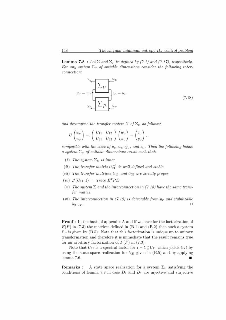
148 The singular minimum entropy H∞ control problem
Lemma 7.8 : Let Σ and ΣP be defined by (7.1) and (7.17), respectively.For any system ΣU of suitable dimensions consider the following inter-connection:
ΣP
ΣU
✛yP
✛
✛uP
✛
❄✻
zU wU
yU = wP zP = uU
(7.18)
and decompose the transfer matrix U of ΣU as follows:
U
(wU
uU
)=:
(U11 U12
U21 U22
)(wU
uU
)=
(zU
yU
),
compatible with the sizes of uU , wU , yU , and zU . Then the following holds:a system ΣU of suitable dimensions exists such that:
(i) The system ΣU is inner
(ii) The transfer matrix U−121 is well-defined and stable
(iii) The transfer matrices U11 and U22 are strictly proper
(iv) J (U11, 1) = Trace ETPE
(v) The system Σ and the interconnection in (7.18) have the same trans-fer matrix.
(vi) The interconnection in (7.18) is detectable from yP and stabilizableby uP . ✷
Proof : In the basis of appendix A and if we have for the factorization ofF (P ) in (7.3) the matrices defined in (B.1) and (B.2) then such a systemΣU is given by (B.5). Note that this factorization is unique up to unitarytransformation and therefore it is immediate that the result remains truefor an arbitrary factorization of F (P ) in (7.3).
Note that U21 is a spectral factor for I −U∼11U11 which yields (iv) by
using the state space realization for U21 given in (B.5) and by applyinglemma 7.6.
Remarks : A state space realization for a system ΣU satisfying theconditions of lemma 7.8 in case D2 and D1 are injective and surjective

7.4 A system transformation 149
respectively is given, without the need of the bases in appendix A, by(B.6).
Combining lemmas 7.5 and 7.8, we find the following theorem:
Theorem 7.9 : Let the systems (7.1) and (7.17) be given. Moreover,let a compensator ΣF of the form (2.4) be given. The following twoconditions are equivalent:
• ΣF is internally stabilizing for Σ such that the closed-loop transfermatrix Gcl is strictly proper and has H∞ norm strictly less than 1.
• ΣF is internally stabilizing for ΣP such that the closed-loop transfermatrix Gcl,P is strictly proper and has H∞ norm strictly less than1.
Moreover, if ΣF satisfies the above conditions then we have
J (Gcl, 1) = J (Gcl,P , 1) + Trace ETPE. ✷
Next, we make another transformation from ΣP to ΣP,Q. This transforma-tion is exactly dual to the transformation from Σ to ΣP . We know thereexists a controller which is internally stabilizing for ΣP which makes theH∞ norm of the closed-loop system strictly less than 1. Therefore if weapply theorem 5.1 to ΣP we find that a unique matrix Y exists such thatG(Y ) ≥ 0 and
(i) rank G(Y ) = rankR(s)Gdi,
(ii) rank(M(Y, s) G(Y )
)= n+ rankR(s)Gdi, ∀ s ∈ C0 ∪ C+,
where
G(Y ) :=
APY + Y AT
P+ EET + Y CT
2,PC2,PY Y CT
1,P+ EDT
1
C1,PY +D1ET D1D
T1
,
M(Y, s) :=
(sI −AP − Y CT
2,PC2,P
−C1,P
),
Gdi(s) := C1,P (sI −AP )−1E +D1.
In lemma 5.5 it has been shown that Y := (I −QP )−1Q satisfies theabove conditions. We factorize G(Y ):
G(Y ) =
(EP,Q
DP,Q
)(ET
P,QDT
P,Q
). (7.19)

150 The singular minimum entropy H∞ control problem
where EP,Q and DP,Q are matrices of suitable dimensions. We define thefollowing system:
ΣP,Q :
xP,Q = AP,QxP,Q + BP,QuP,Q + EP,Qw,
yP,Q = C1,PxP,Q + DP,Qw,
zP,Q = C2,PxP,Q + DPuP,Q,
(7.20)
where AP,Q := AP +Y CT2,PC2,P and BP,Q := B+Y CT
2,PDP . Using theorem
7.9 and a dualized version for the transformation from ΣP to ΣP,Q we canderive the following corollary:
Corollary 7.10 : Let the systems (7.1) and (7.20) be given. Moreover,let a compensator ΣF of the form (2.4) be given. The following twoconditions are equivalent:
• ΣF is internally stabilizing for Σ such that the closed-loop transfermatrix Gcl is strictly proper and has H∞ norm strictly less than 1.
• ΣF is internally stabilizing for ΣP,Q such that the closed-loop trans-fer matrix Gcl,P,Q is strictly proper and has H∞ norm strictly lessthan 1.
Moreover, if ΣF satisfies the above conditions then we have
J (Gcl, 1) = J (Gcl,P,Q, 1) + Trace ETPE + Trace C1,PY C1,P . ✷
From this corollary it is immediate that it is sufficient to investigate ΣP,Q
to prove the results in our main theorem 7.1. This is done in the nextsection.
7.5 (Almost) disturbance decoupling and mini-
mum entropy
The first thing we would like to know is what we gain by our transfor-mation from Σ to ΣP,Q. It turns out that we obtain in this way a systemof the form (7.1) such that part (ii) of theorem 5.1 is satisfied for P = 0and Q = 0. This implies that:
rank
(sI −AP,Q −BP,Q
C2,P DP
)= n+ rank
(C2,P DP
), (7.21)
rank
(sI −AP,Q −EP,Q
C1,P DP,Q
)= n+ rank
(EP,Q
DP,Q
), (7.22)

7.5 (Almost) disturbance decoupling and minimum entropy 151
for all s ∈ C0 ∪ C+. Using these conditions we can apply theorem 2.20.We obtain the following:
Theorem 7.11 : Consider the system (7.1). Assume that the systems(A,B,C2,D2) and (A,E,C1,D1) have no invariant zeros on the imag-inary axis and assume that a controller exists which is such that theclosed-loop system is internally stable and has H∞ norm strictly less than1. The infimum of (7.2), over all internally stabilizing controllers of theform (2.4) which are such that the closed system has H∞ norm strictlyless than 1, is equal to:
Trace ETPE + Trace (ATP + PA+ CT2C2 + PEETP )(I −QP )−1Q
(7.23)
where P and Q are such that part (ii) of theorem 5.1 is satisfied. ✷
Proof : By corollary 7.10 and the non-negativity of the entropy function,the infimum is always larger than or equal to (7.23). Next we choose asequence of controllers ΣF,n satisfying the conditions of theorem 2.20.This is possible because of (7.21) and (7.22). These controllers applied toΣP,Q yield internally stable closed-loop systems and it is straightforwardto check that the closed-loop transfer matrices Gcl,n,P,Q satisfy:
J (Gcl,n,P,Q, 1)→ 0
as n → ∞. By applying corollary 7.10 we find that if we apply thecontrollers ΣF,n to Σ then we find closed-loop systems which are internallystable and the closed-loop transfer matrices Gcl,n are strictly proper, haveH∞ norm less than 1 and satisfy
J (Gcl,n, 1)→ Trace ETPE+
Trace (ATP + PA+ CT2C2 + PEETP )(I −QP )−1Q
as n→∞, which completes the proof of this corollary.
Theorem 7.11 is in fact the main part of theorem 7.1. Exactly when theinfimum of the entropy function is attained is still to be investigated.From the theory of almost disturbance decoupling (see [Tr]), it is well-known that there is often only a non-proper controller which attains the

152 The singular minimum entropy H∞ control problem
infimum (note that because the interconnection should be well-posed itis possible that not even a non-proper controller can attain the infimum).However, we would like to know when it is possible to attain the infimumby a proper controller. Note that the infimum is attained if, and onlyif, we can find a controller for ΣP,Q which makes the closed-loop systeminternally stable and the closed-loop transfer matrix Gcl has H∞ normless than 1 and its entropy is equal to 0. However, the entropy is 0 if, andonly if, Gcl = 0 by lemma 7.2. This reduces our original problem to whatis often called the disturbance decoupling problem with measurementfeedback and internal stability (DDPMS), i.e. the problem of finding astabilizing controller which makes the closed-loop transfer matrix equalto 0 as discussed in section 2.6.
After some extensive calculations the following two equalities can bederived:
Vg(A+ EETP,B,C2,P ,DP ) = Vg(AP,Q, BP,Q, C2,P ,DP )Tg(A+QCT
1C1, EQ, C1,DQ) = (I −QP )Tg(AP,Q, EP,Q, C1,P ,DP,Q)
Applying theorem 2.19 then yields the proof of the final result in theorem7.1.
7.6 Conclusion
In this chapter we have given a complete treatment of the singular min-imum entropy H∞ control problem. We have an explicit formula for theinfimum. Moreover, we can characterize when the infimum is attained.The construction of a controller can be done using some tools from thegeometric approach to control theory. However, this method is too ex-tensive (though straightforward) to discuss in this chapter. Finally wewould like to note that this chapter gives a nice structured approach to“entropy at infinity” with fewer technicalities than [Mu] where entropyat infinity is simply a special yet important case.
A main open problem remains the problem of invariant zeros on theimaginary axis. Moreover, we would like to have results on LQG itselfinstead of the upper bound given by the entropy. A first start has beenmade in [RK] but much more work has to be done. Finally, anotherinteresting extension is the general setup of subsection 1.6.3 where wehave two kinds of disturbances and two kinds of output to be controlled.From one disturbance input to one of the outputs to be controlled wewant to satisfy an H∞ norm bound. For the closed-loop transfer matrixfrom the other disturbance to the other output to be controlled we wantto minimize anH2 norm. In this way we can relate performance criteria to

7.6 Conclusion 153
robustness criteria with much more arbitrary structure for the parameteruncertainty. Some references are given in the introduction of this chapter.
Chapter 8
The finite horizon H∞ controlproblem
8.1 Introduction
Most of the papers on the H∞ control problem mentioned in the previouschapters discuss the “standard” H∞ problem: minimize the L2[0,∞)-induced operator norm of the closed-loop operator over all internally sta-bilizing feedback controllers.
A number of generalizations have appeared recently. One of these isthe minimization of the L2-induced operator norm over a finite horizon(see [Li5, Ta]). As in the infinite horizon H∞ problem, difficulties arise ifthe direct-feedthrough matrices do not satisfy certain assumptions (theso-called singular case). This chapter will use the techniques from chap-ters 4 and 5 to handle this problem for the finite-horizon case.
The following problem will be considered: given a finite-dimensionalsystem on a bounded time-interval [0, T ], together with a positive realnumber γ, find necessary and sufficient conditions for the existence ofa dynamic compensator such that the L2[0, T ]-induced norm of the re-sulting closed-loop operator is smaller than γ. In [Ta] and [Li5] suchconditions were formulated in terms of the existence of solutions to cer-tain Riccati differential equations. Of course, in order to guarantee theexistence of these Riccati differential equations, certain coefficient matri-ces of the system under consideration should have full rank (the regularcase). The present paper addresses the problem formulated above withoutthese full rank assumptions. We find necessary and sufficient conditionsin terms of a pair of quadratic matrix differential inequalities.
The results of this chapter have already appeared in [St7, Tr2]. Thedetailed proof of the results is highly technical and can be found in [St7].This paper discusses time-varying systems which satisfy a number of con-
154

8.2 Problem formulation and main results 155
ditions. These conditions are more or less requirements that all the geo-metric subspaces we use in appendix A and their dual versions, which wecan define for each t, are independent of time. For two important casesthese conditions are always satisfied:
• If the system is time-invariant (i.e. all coefficient matrices are con-stant, independent of time).
• If the problem is regular in the sense as explained above.
In this chapter, contrary to [Li5, Ta], we shall assume that the systemis time-invariant. We shall try to give the main ideas of the proof whichfollows the same lines as the proof of the results on the singular, infinitehorizon,H∞ control problem discussed in the previous chapters. However,we shall not give all the technical details. For this, we refer to [St7]
The outline of this chapter is as follows: in section 8.2 we shall for-mulate our problem and present our main result. In section 8.3 it will benoted that if a controller exists which makes the L2[0, T ]-induced opera-tor norm of the closed-loop operator less than 1 then matrices functionsP and Q exist satisfying a pair of quadratic matrix differential inequali-ties, two corresponding rank conditions and two boundary conditions. Inthe same section we shall introduce a system transformation with the,by now standard, property: a controller “works” for this new system if,and only if, the same controller “works” for the original system. Usingthis transformation we shall show that another necessary condition forthe existence of the desired controller is that P and Q satisfy a cou-pling condition: I − PQ is invertible for all t. In section 8.4 we shallapply a second transformation, dual to the first, which will show thatthe necessary conditions derived are also sufficient. This will be done byshowing that the system we obtained by our two transformations satisfiesthe following condition: for all ε > 0 a controller exists which makes theL2[0, T ]-induced norm of the closed-loop operator less than ε. We shallend the chapter with a couple of concluding remarks.
8.2 Problem formulation and main results
Consider the linear time-invariant system
Σ :
x = Ax + Bu + Ew,
y = C1x + D1w,
z = C2x + D2u.
(8.1)
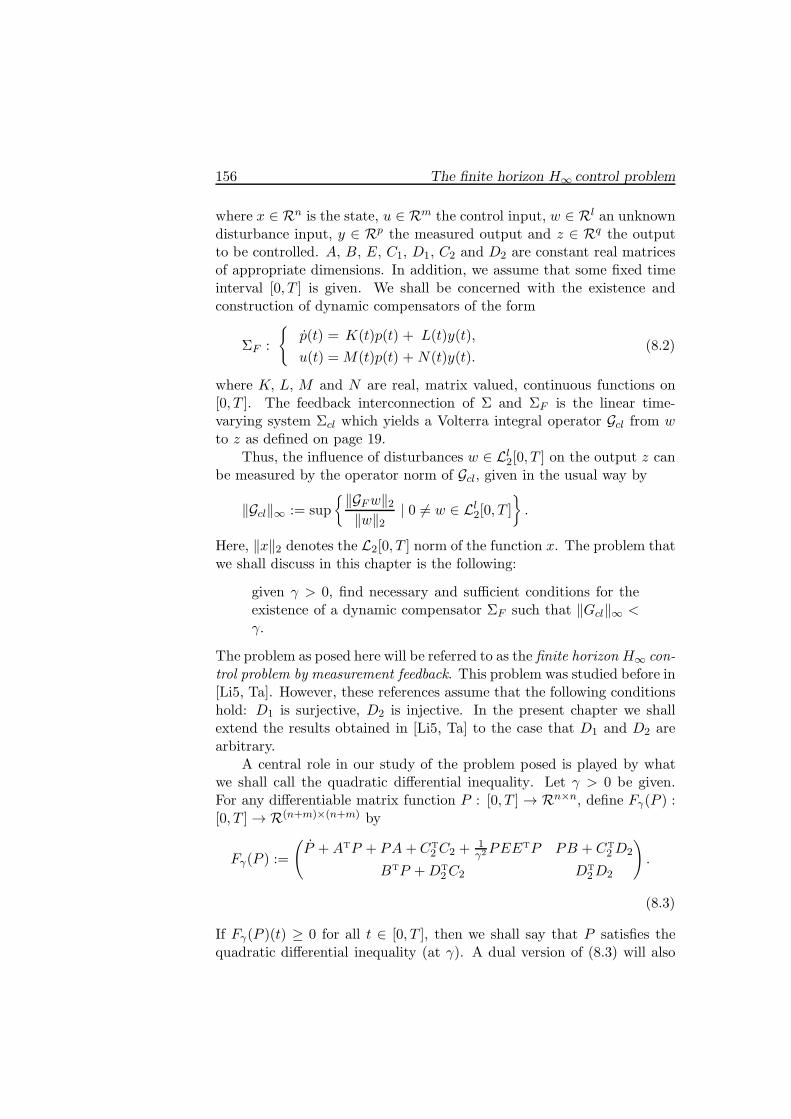
156 The finite horizon H∞ control problem
where x ∈ Rn is the state, u ∈ Rm the control input, w ∈ Rl an unknowndisturbance input, y ∈ Rp the measured output and z ∈ Rq the outputto be controlled. A, B, E, C1, D1, C2 and D2 are constant real matricesof appropriate dimensions. In addition, we assume that some fixed timeinterval [0, T ] is given. We shall be concerned with the existence andconstruction of dynamic compensators of the form
ΣF :
{p(t) = K(t)p(t) + L(t)y(t),u(t) =M(t)p(t) + N(t)y(t).
(8.2)
where K, L, M and N are real, matrix valued, continuous functions on[0, T ]. The feedback interconnection of Σ and ΣF is the linear time-varying system Σcl which yields a Volterra integral operator Gcl from wto z as defined on page 19.
Thus, the influence of disturbances w ∈ Ll2[0, T ] on the output z canbe measured by the operator norm of Gcl, given in the usual way by
‖Gcl‖∞ := sup{‖GFw‖2‖w‖2
| 0 �= w ∈ Ll2[0, T ]}.
Here, ‖x‖2 denotes the L2[0, T ] norm of the function x. The problem thatwe shall discuss in this chapter is the following:
given γ > 0, find necessary and sufficient conditions for theexistence of a dynamic compensator ΣF such that ‖Gcl‖∞ <γ.
The problem as posed here will be referred to as the finite horizon H∞ con-trol problem by measurement feedback. This problem was studied before in[Li5, Ta]. However, these references assume that the following conditionshold: D1 is surjective, D2 is injective. In the present chapter we shallextend the results obtained in [Li5, Ta] to the case that D1 and D2 arearbitrary.
A central role in our study of the problem posed is played by whatwe shall call the quadratic differential inequality. Let γ > 0 be given.For any differentiable matrix function P : [0, T ]→ Rn×n, define Fγ(P ) :[0, T ]→ R(n+m)×(n+m) by
Fγ(P ) :=
(P +ATP + PA+CT
2C2 + 1γ2PEE
TP PB + CT2D2
BTP +DT2C2 DT
2D2
).
(8.3)
If Fγ(P )(t) ≥ 0 for all t ∈ [0, T ], then we shall say that P satisfies thequadratic differential inequality (at γ). A dual version of (8.3) will also

8.2 Problem formulation and main results 157
be important to us: for any differentiable Q : [0, T ] → Rn×n defineGγ(Q) : [0, T ]→R(n+p)×(n+p) by:
Gγ(Q) :=
(−Q+AQ+QAT + EET + 1
γ2QCT2C2Q QCT
1 + EDT1
C1Q+D1ET D1D
T1
).
If Gγ(Q)(t) ≥ 0 for all t ∈ [0, T ] then we shall say that Q satisfies thedual quadratic differential inequality (at γ). In the sequel let
Gci(s) := C2(Is−A)−1B +D2,
Gdi(s) := C1(Is−A)−1E +D1
denote the open-loop transfer matrices from u to z and w to y, respec-tively. We are now ready to state our main result:
Theorem 8.1 : Let γ > 0. The following two statements are equivalent:
(i) A compensator ΣF of the form (8.2) exists such that ‖Gcl‖∞ < γ,
(ii) Differentiable matrix functions P and Q : [0, T ]→Rn×n exist suchthat
(a) Fγ(P )(t) ≥ 0 ∀t ∈ [0, T ] and P (T ) = 0,
(b) rank Fγ(P )(t) = rankR(s)Gci ∀t ∈ [0, T ],
(c) Gγ(Q)(t) ≥ 0 ∀t ∈ [0, T ] and Q(0) = 0,
(d) rank Gγ(Q)(t) = rankR(s)Gdi ∀t ∈ [0, T ],
(e) γ2I −Q(t)P (t) is invertible for all t ∈ [0, T ]. ✷
The aim of this chapter is to outline the main steps and ideas involved ina proof of the latter theorem. For a more detailed discussion we wouldlike to refer to [St7].
It can be shown that, in general, if Fγ(P ) ≥ 0 on [0, T ] then
rank Fγ(P )(t) ≥ rankR(s)Gci on[0, T ]
and, likewise, Gγ(Q) ≥ 0 on [0, T ] then
rank Gγ(Q)(t) ≥ rankR(s)Gdi on[0, T ]
This means that conditions (a) and (b) can be reformulated as: P isa rank-minimizing solution of the quadratic differential inequality at γ,satisfying the end-condition P (T ) = 0. A similar statement is valid for

158 The finite horizon H∞ control problem
the conditions (c),(d). It can also be shown that if P satisfies (a), (b)then it is unique. Also, this unique solution turns out to be symmetricfor all t ∈ [0, T ]. The same holds for Q satisfying (c) and (d).
It can be shown that for the special case whenD1 andD2 are assumedto be surjective and injective, respectively, our theorem 8.1 specializes tothe results obtained before in [Li5, Ta].
It can also be shown that if the conditions in the statement of 8.1 part(ii) indeed hold, then it is always possible to find a suitable compensatorwith dynamic order equal to n, the dynamic order of the system to becontrolled.
8.3 Completion of the squares
In this section we shall outline the proof of the implication (i) ⇒ (ii) oftheorem 8.1. Consider the system Σ. Our starting point is the followinglemma:
Lemma 8.2 : Let γ > 0. Assume that there exists δ < γ such that forall w ∈ Ll2[0, T ] we have
inf {‖zu,w‖2 − δ‖w‖2 |u ∈ Lm2 [0, T ]} ≤ 0. (8.4)
Then a differentiable matrix function P : [0, T ] → Rn×n exists suchthat P (T ) = 0, Fγ(P )(t) ≥ 0 and rank Fγ(P )(t) = rankR(s)Gci for allt ∈ [0, T ]. ✷
Proof : A proof of this can be given by using the techniques from chapter3 (solve the regular case) and 4 (extend to the singular case).
Now, assume that the condition (i) in the statement of theorem 8.1 holds,i.e. assume that a dynamic compensator ΣF exists such that ‖Gcl‖∞ =:δ < γ. Therefore condition (8.4) is satisfied: let w ∈ Ll2[0, T ] and let zbe the closed-loop output with x(0) = 0 and p(0) = 0. Then z = zu,w,where u is the output of ΣF . Clearly
‖z‖2‖w‖2
≤ ‖Gcl‖∞
and hence ‖zu,w‖2−δ‖w‖2 ≤ 0. Then also the infimum in (8.4) is less thanor equal to 0. Therefore we may conclude that, indeed, a differentiable

8.3 Completion of the squares 159
matrix function P exists that satisfies conditions (a) and (b) of theorem8.1.
The fact that (c) and (d) of theorem 8.1 also hold for a certain matrixfunctionQ can be proven by the following dualization argument. Considerthe dual system
Σ′ :
ξ = ATξ + CT
1 ν + CT2 d,
η = BTξ + DT2 d,
ζ = ETξ + DT1 ν.
and apply to Σ′ the time-varying compensator
Σ′F :
{q(t) = KT(T − t)q(t) +MT(T − t)η(t),ν(t) = LT(T − t)q(t) + NT(T − t)η(t).
It can be shown that if we denote by Gcl the closed-loop operator ofΣ′×Σ′
F (with ζ(0) = 0, q(0) = 0), and if G3cl denotes the adjoint operatorof Gcl then the following equality holds:
Gcl = R ◦ G3cl ◦R, (8.5)
where R denotes the time-reversal operator (Rx)(t) := x(T − t). Now, if‖Gcl‖∞ < γ then also ‖G3cl‖∞ < γ and therefore, by (8.5), ‖Gcl‖∞ < γ. Wecan therefore conclude that the quadratic differential inequality associatedwith Σ′ has an appropriate solution, say P (t), on [0, T ]. By definingQ(t) := P (T − t) we obtain a function Q that satisfies (c) and (d) oftheorem 8.1.Finally, we have to show that condition (e) of theorem 8.1 holds. Weshall need the following lemma:
Lemma 8.3 : Assume that P : [0, T ]→Rn×n exists such that Fγ(P )(t) ≥0, ∀t ∈ [0, T ], and rank Fγ(P )(t) = rankR(s)G, ∀t ∈ [0, T ]. Then contin-uous matrix functions C2,P and DP exist such that for all t ∈ [0, T ]
Fγ(P )(t) =
(CT
2,P(t)
DTP(t)
)(C2,P (t) DP (t)
). (8.6)
✷
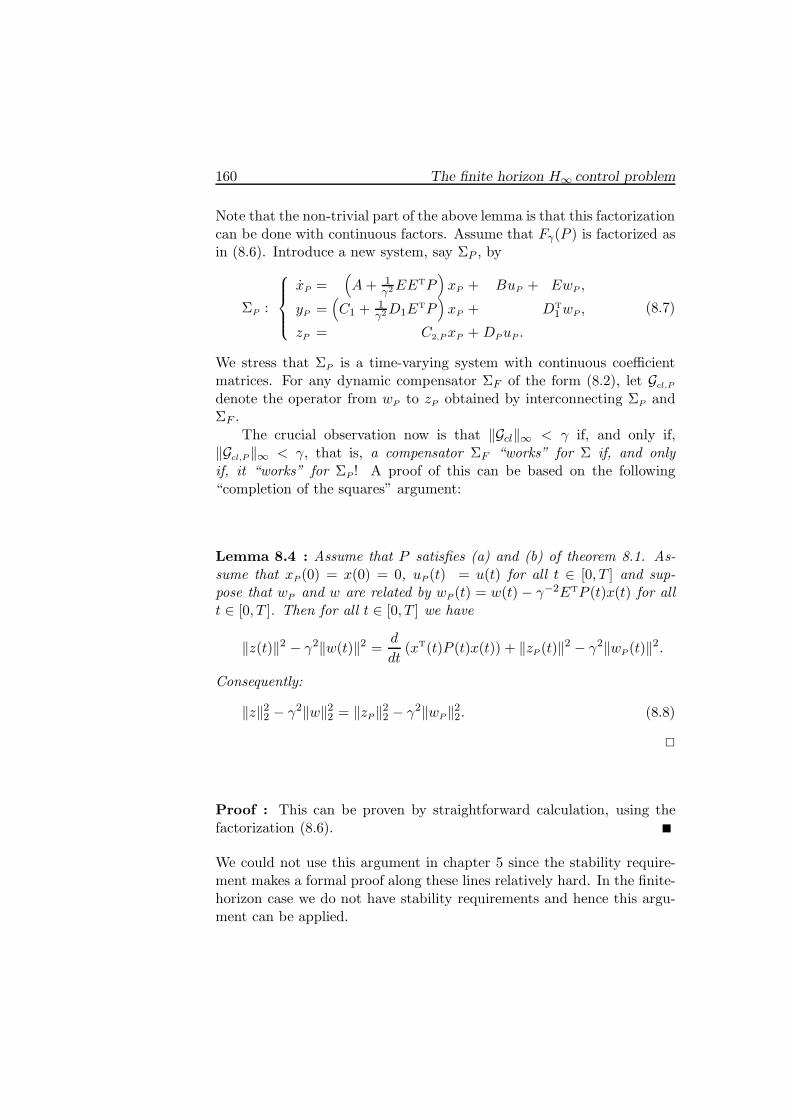
160 The finite horizon H∞ control problem
Note that the non-trivial part of the above lemma is that this factorizationcan be done with continuous factors. Assume that Fγ(P ) is factorized asin (8.6). Introduce a new system, say ΣP , by
ΣP :
xP =
(A+ 1
γ2EETP
)xP + BuP + EwP ,
yP =(C1 + 1
γ2D1ETP
)xP + DT
1wP ,
zP = C2,PxP + DPuP .
(8.7)
We stress that ΣP is a time-varying system with continuous coefficientmatrices. For any dynamic compensator ΣF of the form (8.2), let Gcl,P
denote the operator from wP to zP obtained by interconnecting ΣP andΣF .
The crucial observation now is that ‖Gcl‖∞ < γ if, and only if,‖Gcl,P‖∞ < γ, that is, a compensator ΣF “works” for Σ if, and onlyif, it “works” for ΣP ! A proof of this can be based on the following“completion of the squares” argument:
Lemma 8.4 : Assume that P satisfies (a) and (b) of theorem 8.1. As-sume that xP (0) = x(0) = 0, uP (t) = u(t) for all t ∈ [0, T ] and sup-pose that wP and w are related by wP (t) = w(t) − γ−2ETP (t)x(t) for allt ∈ [0, T ]. Then for all t ∈ [0, T ] we have
‖z(t)‖2 − γ2‖w(t)‖2 = d
dt(xT(t)P (t)x(t)) + ‖zP (t)‖2 − γ2‖wP (t)‖2.
Consequently:
‖z‖22 − γ2‖w‖22 = ‖zP‖22 − γ2‖wP‖22. (8.8)
✷
Proof : This can be proven by straightforward calculation, using thefactorization (8.6).
We could not use this argument in chapter 5 since the stability require-ment makes a formal proof along these lines relatively hard. In the finite-horizon case we do not have stability requirements and hence this argu-ment can be applied.

8.3 Completion of the squares 161
Theorem 8.5 : Let P satisfy (a) and (b) of theorem 8.1. Let ΣF be adynamic compensator of the form (8.2). Then
‖Gcl‖∞ < γ ⇔ ‖Gcl,P‖∞ < γ. ✷
Proof : Assume that ‖Gcl,P‖∞ < γ and consider the interconnection ofΣ and ΣF .
Σ
ΣF
❄
✛
✻
✛
y
z w
u
ΣP
ΣF
❄
✛
✻
✛
yP
zP wP
uP
Let 0 �= w ∈ Ll2[0, T ], let x be the corresponding state trajectory of Σ anddefine wP := w − γ−2ETPx. Then clearly yP = y, xP = x and thereforeuP = u. This implies that the equality (8.7) holds. We also have
‖zP‖22 − γ2‖wP‖22 ≤ (‖Gcl,P‖2∞ − γ2)‖wP‖22. (8.9)
Next, note that the mapping wP → wP + γ−2ETPxP defines a boundedoperator from Ll2[0, T ] to Ll2[0, T ]. Hence a constant µ > 0 exists suchthat ‖wP‖22 < µ‖w‖22. Define δ > 0 by δ2 := γ2 − ‖Gcl,P‖2∞. Combining(8.7) and (8.8) then yields
‖z‖22 − γ2‖w‖22 ≤ −δ2µ‖w‖22.
Obviously, this implies that ‖Gcl‖2∞ ≤ γ2 − δ2µ < γ2.
We shall now prove that condition (e) of theorem 8.1 holds. Again assumethat ΣF yields ‖Gcl‖∞ < γ. By applying a version of lemma 8.2 for time-varying systems it can then be proven that the dual quadratic differentialinequality associated with ΣP :
Gγ(Y ) :=
(−Y +APY + Y AT
P+ EET + 1
γ2Y CT2,PC2,PY Y CT
1,P+ EDT
1
C1,PY +D1ET D1D
T1
)≥ 0
has a solution Y (t) on [0, T ], satisfying Y (0) = 0 and
rank Gγ(Y )(t) = rankR(s)
(Is−AP (t) −EC1,P (t) D1
)− n (8.10)

162 The finite horizon H∞ control problem
for all t ∈ [0, T ]. Here, we have denoted AP = A + γ−2EETP andC1,P = C1 + γ−2D1E
TP . Furthermore, it can be shown that Y is uniqueon each interval [0, t1] (t1 ≤ T ). On the other hand, it can be proven thaton each interval [0, t1] on which I − QP is invertible, the function Y :=(I − QP )−1Q satisfies Gγ(Y )(t) ≥ 0, Y (0) = 0 and the rank condition(8.10). Thus on any such interval [0, t1] we must have Y (t) = Y (t).Clearly, since Q(0) = 0, t1 : 0 < t ≤ T exists such that I − QP isinvertible on [0, t). Assume now that t1 > 0 is the smallest real numbersuch that I −Q(t1)P (t1) is not invertible. Then on [0, t1) we have
Q(t) = (I −Q(t)P (t)) Y (t)
and hence, by continuity
Q(t1) = (I −Q(t1)P (t1)) Y (t1). (8.11)
x �= 0 exists such that xT(I − Q(t1)P (t1)) = 0. By (8.11) this yieldsxTQ(t1) = 0 whence xT = 0, which is a contradiction. We must concludethat I −Q(t)P (t) is invertible for all t ∈ [0, T ].
This completes our proof of the implication (i) ⇒ (ii) of theorem 8.1
8.4 Existence of compensators
In the present section we shall sketch the main ideas of our proof of theimplication (ii)⇐ (i) of theorem 8.1. The main idea is as follows: startingfrom the original system Σ we shall define a new system, ΣP,Q, which hasthe following important properties:
(1 ) Let ΣF be any compensator. The closed-loop operator Gcl of theinterconnection Σ × ΣF satisfies ‖Gcl‖∞ < γ if, and only if, theclosed-loop operator of ΣP,Q×ΣF , say Gcl,P,Q, satisfies ‖Gcl,P,Q‖∞ <γ.
(2 ) The system ΣP,Q is almost disturbance decouplable by dynamicmeasurement feedback, i.e. for all ε > 0 there exists ΣF suchthat ‖Gcl,P,Q‖∞ < ε.
Property (1) states that a compensator ΣF “works” for Σ if, and only if,it “works” for ΣP,Q. On the other hand, property (2) states that, indeed,there is a compensator ΣF that ”works” for ΣP,Q: take any ε ≤ γ andtake a compensator ΣF such that ‖Gcl,P,Q‖∞ < ε. Then by, property (1),‖Gcl‖∞ < γ so ΣF works for Σ. This would clearly establish a proof ofthe implication (ii) ⇐ (i) in theorem 8.1.

8.4 Existence of compensators 163
We shall now describe how the new system ΣP,Q is defined. Assumethat P and Q exist satisfying (a) to (e) of theorem 8.1. Apply lemma8.3 to obtain a continuous factorization (8.6) of Fγ(P ) and let the systemΣP be defined by (8.7). Next, consider the dual quadratic differentialinequality Gγ(Y ) ≥ 0 associated with the system ΣP , together with theconditions Y (0) = 0 and the rank condition (8.10). As was already notedin the previous section, the conditions (c), (d) and (e) assure that thereis a unique solution Y on [0, T ] (In fact, Y (t) = (γ2I−Q(t)P (t))−1Q(t)).Now, it can be shown that there exists a factorization
Gγ(Y )(t) =
(EP,Q(t)DP,Q(t)
)(ET
P,Q(t) DT
P,Q(t)
),
with EP,Q and DP,Q continuous on [0, T ]. Denote
AP,Q(t) := AP (t) + Y (t)CT2,P (t)C2,P (t),
BP,Q(t) := B + Y (t)CT2,P (t)DP (t).
Then, introduce the new system ΣP,Q by:
ΣP,Q :
xP,Q = AP,QxP,Q + BP,QuP,Q + EP,Qw,
yP,Q = C1,PxP,Q + DP,Qw,
zP,Q = C2,PxP,Q + DPuP,Q,
Again, ΣP,Q is a time-varying system with continuous coefficient matrices.We note that ΣP,Q is in fact obtained by first transforming Σ into ΣP andby subsequently applying the dual of this transformation to ΣP . Weshall now first show that property (1) above holds. If ΣF is a dynamiccompensator, then let Gcl,P,Q be the closed-loop operator from wP,Q tozP,Q in the interconnection of ΣP,Q with ΣF :
Σ
ΣF
❄
✛
✻
✛
y
z w
u
ΣP,Q
ΣF
❄
✛
✻
✛
yP,Y
zP,Y wP,Y
uP,Y
Recall that Gcl denotes the closed-loop operator from w to z in the inter-connection of Σ and ΣF . We have the following:

164 The finite horizon H∞ control problem
Theorem 8.6 :
‖Gcl‖∞ < γ ⇔ ‖Gcl,P,Q‖∞ < γ. ✷
Proof : Assume that ΣF yields ‖Gcl‖∞ < γ. By theorem 8.5 then also‖Gcl,P‖∞ < γ, i.e. ΣF interconnected with ΣP (given by (8.7)) also yieldsa closed-loop operator with norm less than γ. It is easy to see that thedual compensator Σ′
F (see section 8.3), interconnected with the dual ofΣP :
Σ′P,Q :
ξ = ATP(T − t)ξ + CT
1,P(T − t)ν + CT
2,P(T − t)d
η = BTξ + DTP(T − t)d
ζ = ETξ + DT1 ν
yields a closed-loop operator Gcl,P (from d to ζ) with ‖Gcl,P‖∞ < γ. Now,the quadratic differential inequality associated with Σ′
Pis the transposed,
time-reversed version of the inequality Gγ(Y ) ≥ 0 and therefore has aunique solution Y (t) = Y (T − t) such that Y (T ) = 0 and the correspond-ing rank condition (8.10) holds. By applying theorem 8.5 to the systemΣ′
Pwe may then conclude that the interconnection of Σ′
F with the dualΣ′
P,Qof ΣP,Q yields a closed-loop operator with norm less than γ. Again
by dualization we then conclude that ‖Gcl,P,Q‖∞ < γ. The converse im-plication is proven analogously.
Property (2) is stated formally in the following theorem:
Theorem 8.7 : For all ε > 0 a time-varying dynamic compensator ΣF
exists such that ‖Gcl,P,Q‖∞ < ε. ✷
Due to space limitations, for a proof of the latter theorem we refer to[St7]. The main difficulty is that ΣP,Q is time-varying and therefore itis necessary to derive a time-varying version of theorem 2.20 (we do notneed (2.48) but we do need (2.47)). The basic steps are all the same butthe proof is based on [Tr, Theorem 3.25] of which we had to derive atime-varying version.
By combining theorems 8.6 and 8.7 we immediately obtain a proof ofthe implication (ii) ⇐ (i) in theorem 8.1.
8.5 Conclusion 165
8.5 Conclusion
In this chapter we have studied the finite horizon H∞ control problemby dynamic measurement feedback. We have noted that the results ob-tained can be specialized to re-obtain results that were obtained before(see [Li5, Ta]). The development of our theory runs analogously to thetheory developed in chapters 4 and 5 around the standardH∞ control pro-blem (the infinite horizon version of the problem studied in the presentchapter). In the latter chapters the main tools are the so-called quadraticmatrix inequalities, the algebraic versions of the differential inequalitiesused in the present paper. It should be noted that the geometric approachfrom appendix A is not well-suited to treat time-varying systems. Thisis why we cannot treat the time-varying case as in [Li5, Ta]. The formalproof for the results in this chapter is also highly technical, mainly due tothe fact that the systems ΣP and ΣP,Q are time-varying. The reason whythe approach via appendix A still works is that the singular structure ofΣP and ΣP,Q is time-invariant. A major open problem is how to treat thetime-varying singular H∞ or LQG control problem. A different approachwill be needed to derive the general result.
Chapter 9
The discrete time full-informationH∞ control problem
9.1 Introduction
As already mentioned in the previous chapters, in recent years a consider-able number of papers have appeared on theH∞ optimal control problem.However, most of these papers discuss the continuous time case. In thenext two chapters we shall discuss the discrete time case.
In the papers on H∞ control with continuous time several methodswere used to solve theH∞ control problem as discussed in section 5.1. Re-cently, a paper has appeared solving the discrete timeH∞ control problemusing frequency-domain techniques (see [Gu]). The polynomial approachhas also been applied to discrete time systems (see [Gri]). In addition,a couple of papers have appeared using a time-domain approach (see[Bas, Li4, Ya]).
With respect to the papers which use a time-domain approach itshould be noted that the references [Bas, Li4, Ya] do not contain a proof ofthe results obtained for the infinite horizon case and the papers [Bas, Ya]make a number of extra assumptions on the system under consideration.In [Bas, Li4, Ya] the authors first investigate the finite horizon problemand then derive a solution of the infinite horizon problem by consideringit as a kind of limiting case as the endpoint tends to infinity.
In contrast, in the next two chapters we investigate the infinite hori-zon case using a direct approach. We shall use time-domain techniqueswhich are reminiscent of those used in chapter 3 and the paper [Ta] whichdeal with the continuous time case. The method used in the next twochapters was derived independently of [Bas, Li4, Ya] and has already ap-peared in [St5, St6]. After the appearance of the above papers, severalnew papers and a book appeared on this subject using a state space ap-
166

9.1 Introduction 167
proach (see e.g. [BB, Ig, Wa]). Very recently the J-spectral factorizationapproach has also been extended to discrete time systems (see [LMK]).
In this chapter we assume that we deal with the special cases thateither both disturbance and state are available for feedback or only thestate is available for feedback. This distinction has to be made sincethere is a more essential difference between these two cases than in thecontinuous time case. The more general case of measurement feedback isdiscussed in the next chapter.
The assumptions we shall make are weaker than the assumptionsmade in [Gu, Ya] and the same as the ones made in [Li4]. For the full-information case we have to make two assumptions which are exactly thediscrete time analogues of the assumptions made in the regular continuoustimeH∞ control problem as discussed in chapter 3. Firstly, the subsystemfrom control input to output should be left-invertible, and secondly, thissubsystem should have no invariant zeros on the unit circle.
As in the regular continuous time H∞ problem the necessary and suf-ficient conditions for the existence of an internally stabilizing controllersuch that the closed-loop system has H∞ norm less than 1 involve a posi-tive semi-definite stabilizing solution of a given algebraic Riccati equation.However, other than for the continuous time case, P has to satisfy an ad-ditional assumption: a matrix depending on P should be positive definite(in the continuous time case there also was a matrix which should bepositive definite but in that case this matrix was independent of P ).
Another difference with the continuous time case is that in the dis-crete time case, even if D2 = 0, we cannot always achieve our goal with astatic state feedback. In general, we also need a static feedback depend-ing on the disturbance. Moreover, in the continuous time case we couldnot do better by allowing for non-causal compensators. This is not truein the discrete time case.
The outline of this chapter is as follows: in section 9.2 we shall formu-late the problem and give the main results. In section 9.3 we shall derivenecessary conditions under which an internally stabilizing feedback existswhich makes the H∞ norm less than 1. In section 9.4 we shall show thatthese conditions are also sufficient. After that, in section 9.5 we shall givebut not prove some results on the discrete algebraic Riccati equation. Weshall investigate properties like uniqueness of solutions and methods tocalculate the solutions. We shall end with some concluding remarks insection 9.6.

168 The discrete time full-information case
9.2 Problem formulation and main results
We consider the following shift-invariant system:
Σ :
{σx = Ax + Bu + Ew,
z = Cx + D1u + D2w,(9.1)
where for each k, x(k) ∈ Rn is the state, u(k) ∈ Rm is the control input,w(k) ∈ Rl is the unknown disturbance and z(k) ∈ Rp is the output to becontrolled. Moreover, A,B,E,C,D1 and D2 are matrices of appropriatedimensions. Our objective is to find a compensator ΣF described by astatic feedback law u(k) = F1x(k) + F2w(k) such that the closed-loopsystem is internally stable and for the closed-loop system the 92-inducedoperator norm from disturbance w to the output z is less than 1, i.e. theH∞ norm of the closed-loop system is less than 1.
In this chapter we shall derive necessary and sufficient conditions forthe existence of a suitable compensator ΣF . Moreover, in the case thatsuch a compensator exists we give an explicit formula for one static feed-back law which yields a closed-loop system which is internally stable andwhich has H∞ norm less than 1. We shall also derive similar conditionsfor the existence of a suitable static state feedback. A characterization ofall suitable dynamic compensators will be given in section 10.5.
We first give a definition:
Definition 9.1 : An function f : 92 → 92, w → f(w) is called causal iffor any w1, w2 ∈ 92 and k ∈ N :
w1|[0,k] = w2|[0,k] ⇒ f(w1)|[0,k] = f(w2)|[0,k].
Such a function f is called strictly causal if for any w1, w2 ∈ 92 and k ∈ Nwe have
w1|[0,k−1] = w2|[0,k−1] ⇒ f(w1)|[0,k] = f(w2)|[0,k]. ✷
A controller of the form (2.9) always defines a causal operator. In thecase that N = 0 this operator is strictly causal.
We now formulate our main result:
Theorem 9.2 : Consider the system (9.1) and assume that the sys-tem (A,B,C,D1) has no invariant zeros on the unit circle and is left-invertible. The following three statements are equivalent:

9.2 Problem formulation and main results 169
(i) A compensator ΣF described by a static feedback law of the formu = F1x+ F2w exists such that the closed-loop system is internallystable and has H∞ norm less than 1, i.e. the closed-loop transfermatrix GF satisfies ‖GF ‖∞ < 1.
(ii) (A,B) is stabilizable and for the system (9.1) a causal operator f :9l2 → 9m2 and δ < 1 exist such that for all w ∈ 9l2 with u = f(w) wehave xu,w ∈ 9n2 and ‖zu,w‖2 ≤ δ‖w‖2.
(iii) A symmetric matrix P ≥ 0 exists such that(a) V > 0, R > 0, (9.2)
where
V := DT1D1 +BTPB,
R := I −DT2D2 − ETPE
+(ETPB +DT
2D1
)V −1
(BTPE +DT
1D2
).
This implies that the matrix G(P) is invertible, where:
G(P ) :=
(DT
1D1 DT1D2
DT2D1 DT
2D2 − I
)+
(BT
ET
)P(B E
). (9.3)
(b) P satisfies the following discrete algebraic Riccati equation:
P = ATPA+ CTC
−(BTPA+DT
1C
ETPA+DT2C
)T
G(P )−1
(BTPA+DT
1C
ETPA+DT2C
). (9.4)
(c) The matrix Acl is asymptotically stable, where:
Acl := A−(B E
)G(P )−1
(BTPA+DT
1C
ETPA+DT2C
). (9.5)
Moreover, in the case that P satisfies part (iii), then the compensator ΣF
described by the static feedback law u(k) = F1x(k) + F2w(k) where
F1 := − (DT1D1 +BTPB)−1 (BTPA+DT
1C) , (9.6)F2 := − (DT
1D1 +BTPB)−1 (BTPE +DT1D2) , (9.7)
satisfies the requirements in part (i). ✷

170 The discrete time full-information case
Remarks :
(i) Necessary and sufficient conditions under which we can find an inter-nally stabilizing feedback which makes the H∞ norm of the closed-loop system less than some, a priori given, upper bound γ can easilybe derived from theorem 9.2 by scaling. We only prove the resultfor D2 = 0. The general result can be proven along the same linesand this proof can be found in [St6].
(ii) Note that part (ii) of theorem 9.2 is equivalent to the requirementthat a causal operator f exists such that the feedback law u =f(x,w) satisfies part (ii). This follows from the fact that, afterapplying the feedback, there exists a causal operator g mapping wto x and therefore we could have started with the causal operatoru = f (g(w), w) in the first place. Conversely if we have the feedbacku = f(w), then we define f1(x,w) := f(w) which then satisfies therequirements of the reformulated part (ii).
(iii) In the continuous time case (except for the singular case with D2 �=0) we could not really do better when minimizing the H∞ norm ofthe closed-loop system under the constraint of internal stability byallowing for non-causal feedbacks. This is not true in the discretetime case. Consider, e.g. the following system:
σx =
(0 10 0
)x +
(010
)u +
(10
)w,
z =
1 00 10 0
x +
001
u.
The feedback u = −σw/10 makes the H∞ norm of the closed-loopsystem equal to 0.1. On the other hand, by a causal feedback wecannot make the H∞ norm of the closed-loop system less than 1.
(iv) If we compare these conditions with the conditions for the contin-uous time case as given in chapter 3 we note that condition (9.2)(which is comparable to the condition (3.2) in theorem 3.1) now de-pends on P and is still present if D2 = 0. A simple example showingthat this assumption is not superfluous is given by the system:σx = u + 2w,
z =
(10
)x +
(01
)u.

9.2 Problem formulation and main results 171
No feedback ΣF satisfying part (i) of theorem 9.2 exists but thereis a positive semi-definite matrix P satisfying (9.4) and such thatAcl = 0 and hence asymptotically stable, namely P = 1. Howeverfor this P we have R = −1.
The general outline of the proof will be reminiscent of the proof givenin [Ta] and chapter 3 for the continuous time case. The extra condition(9.2), the invertibility of (9.3) and the requirement of left-invertibilityinstead of assuming that D1 is injective will give rise to a substantialincrease in the amount of intricacies in the proof.
From the above result we can easily derive necessary and sufficientconditions when the system (A,B,C,D) has H∞ norm strictly less than1. This is stated in the following corollary:
Corollary 9.3 : Let the system (A,B,C,D) be given with A stable. Thecorresponding transfer matrix G has H∞ norm strictly less than 1 if, andonly if, there exists a matrix P ≥ 0 such that:
• N := I −DTD −BTPB > 0,
• P = ATPA+CTC + (ATPB + CTD)N−1(BTPA+DTC), and
• A+BN−1(BTPA+DTC) is asymptotically stable. ✷
As in the continuous time case it is interesting to know whether we reallyneed the disturbance feedback component or not. The following theoremgives necessary and sufficient conditions under which we can obtain in-ternal stability and an H∞ norm of the closed-loop system less than 1 byusing a static state feedback.
Theorem 9.4 : Consider the system (9.1) and assume that (A,B,C,D1)has no invariant zeros on the unit circle and is left-invertible. The fol-lowing statements are equivalent:
(i) A compensator ΣF described by a static state feedback law existssuch that the closed-loop system is internally stable and has H∞ normless than 1, i.e. the closed-loop transfer matrix GF satisfies ‖GF ‖∞ <1.
(ii) A symmetric matrix P ≥ 0 exists such that

172 The discrete time full-information case
(a) We have
DT1D1 +BTPB > 0,
R1 := I −DT2D2 − ETPE > 0. (9.8)
This implies that the matrix G(P) defined by (9.3) is invertible.
(b) P satisfies the discrete algebraic Riccati equation (9.4).
(c) The matrix Acl defined by (9.5) is asymptotically stable.
Moreover, in the case that P satisfies part (ii), then the compensator ΣF
described by the static feedback law u(k) = Fx(k) where
F := H−1(BTPA+DT
1C +(BTPE +DT
1D2
)R−1
1
(ETPA+DT
2C))
(9.9)
satisfies the requirements in part (i) where
H := BTPB +DT1D1 +
(BTPE +DT
1D2
)R−1
1
(ETPB +DT
2D1
). ✷
Remarks : Note that the only difference with the conditions of theorem9.2 is that the condition R > 0 is replaced by the condition (9.8). Notethat the latter condition indeed implies R > 0.
In the continuous time case we only needed the extra conditionDT
2D2 < I. This is not sufficient in discrete time as can be seen from thefollowing system:{
σx = u + 1/2w,z = 8x + u.
The matrix P = 84 satisfies the conditions in part (iii) of theorem 9.2but condition (9.8) is not satisfied. By state feedback the H∞ norm of theclosed-loop system cannot be made less than 3 while maintaining internalstability. On the other hand with disturbance feedback we can make theH∞ norm equal to 1/2.
The above theorem will only be proven for the special case that D2 =0. This is done to make the formulae more tractable. It yields no extradifficulties to extend the proof to the general case.
9.3 Existence of a stabilizing solution of the Ric-
cati equation
In this section we shall show that the existence of a causal operator fand δ < 1 satisfying part (ii) of theorem 9.2 implies that a positive semi-definite solution of the discrete algebraic Riccati equation (9.4) exists

9.3 A solution of the Riccati equation 173
such that (9.5) is asymptotically stable and (9.2) is satisfied. We alsoprove the implication (i) ⇒ (ii) of theorem 9.4. As mentioned before weshall assume throughout the next two sections that D2 = 0. The methodused has a great similarity with the proof given in section 3.4. We shallassume that
DT1C = 0, (9.10)
for the time being and we shall derive the more general statement later.Note that part (iii) of the remarks after theorem 9.2 guarantees that,contrary to the continuous time case, we have to be concerned with causaldependence of u on w. In order to prove the existence of the desired Pwe shall investigate the following sup-inf problem:
C∗(ξ) := supw∈4l2
infu
{‖zu,w,ξ‖22 − ‖w‖22 | u ∈ 9m2 such that xu,w,ξ ∈ 9n2
},
(9.11)
for arbitrary initial state ξ. It turns out that the conditions of part (ii)of theorem 9.2 imply that C∗(ξ) is finite for every ξ. Moreover, it will beshown that, as in section 3.4, a P ≥ 0 exists such that C∗(ξ) = ξTPξ.At the end of this section we then prove that this P exactly satisfiesconditions (a)–(c) of theorem 9.2. We shall first infimize, for given w ∈ 92and ξ ∈ Rn, the function ‖zu,w,ξ‖22 − ‖w‖22 over all u ∈ 92 for whichxu,w,ξ ∈ 92. After that we shall maximize over w ∈ 92.
As in chapter 3 our proof is based on Pontryagin’s maximum prin-ciple. We shall use the ideas from [LM], together with our stability re-quirement xu,w,ξ ∈ 92 to adapt the proof to the infinite horizon discretetime case.
We start by constructing a solution of the adjoint Hamilton–Jacobiequation which is a natural starting point if one wants to use Pontryagin’smaximum principle.
Let L be such that DT1D1+BTLB is invertible and such that L is the
positive semi-definite solution of the following discrete algebraic Riccatiequation:
L = ATLA+ CTC −ATLB (DT1D1 +BTLB)−1
BTLA, (9.12)
for which
AL := A−B (DT1D1 +BTLB)−1
BTLA,
is asymptotically stable. The existence of such L is guaranteed under theassumption that (A,B,C,D1) has no invariant zeros on the unit circle

174 The discrete time full-information case
and is left-invertible and, moreover, (A,B) is stabilizable (see [Si]). Wedefine
r(k) := −∞∑i=k
[X1AT]i−k
X1LEw(i), (9.13)
where
X1 := I − LB (DT1D1 +BTLB)−1
BT.
Note that r is well-defined since the matrix AL = XT1A is asymptotically
stable which implies that X1AT is asymptotically stable. Next we define
the functions y, x and η by:
y := M−1BT [ATσr − LEw] , (9.14)σx = ALx+By + Ew, x(0) = ξ, (9.15)η := −X1LAx+ r, (9.16)
where M := DT1D1 + BTLB. Since AL and X1A
T are asymptoticallystable, it can be checked straightforwardly that, given ξ ∈ Rn and w ∈ 9l2,we have r, x, η ∈ 92.
After some standard calculations, we find the following lemma:
Lemma 9.5 : Let ξ ∈ Rn and w ∈ 9l2 be given. The function η ∈ 9n2 is asolution of the following backward difference equation:
σ−1η = ATη − CTCx, limk→∞
η(k) = 0. (9.17)
Here η is extended to a function from N ∪{−1} to Rn by choosing η(−1)such that (9.17) is satisfied. ✷
In the statement of Pontryagin’s maximum principle this equation is theso-called “adjoint Hamilton–Jacobi equation” and η is called the “adjointstate variable”. We have constructed a solution to this equation and weshall show that this η indeed yields a minimizing u. Note the differencewith the continuous time case where we could derive a differential equa-tion forward in time, while in discrete time we can only derive a differenceequation forward in time when A is invertible. To prevent this kind ofdifficulty it is assumed in [Gu] that A is invertible. The proof that ηyields a minimizing u is adapted from the proof of lemma 3.4:

9.3 A solution of the Riccati equation 175
Lemma 9.6 : Let the system (9.1) be given. Moreover let w and ξ befixed. Then
u := − (DT1D1 +BTLB)−1BTLAx+ y
= arg infu{ ‖zu,w,ξ‖2 | u ∈ 9m2 such that xu,w,ξ ∈ 9n2 } . ✷
Proof : It is easy to check that x = xu,w,ξ. Define
JT (u) :=T∑i=0
‖Cxu,w,ξ(i) +D1u(i)‖2.
Let u ∈ 9m2 be an arbitrary control input such that xu,w,ξ ∈ 9n2 . We find
JT (u)− JT−1(u)− 2ηT(T )x(T + 1) + 2ηT(T − 1)x(T ) =
‖Cx(T )‖2 + [DT1D1u(T )− 2BTη(T )]T u(T )
−2ηT(T )Ew(T ) − 2xT(T )CTCx(T ).
We also find
JT (u)− JT−1(u)− 2ηT(T )x(T + 1) + 2ηT(T − 1)x(T ) =
−‖Cx(T )‖2 + [DT1D1u(T )− 2BTη(T )]T u(T )− 2ηT(T )Ew(T ).
Hence, if we sum the last two equations from zero to infinity and subtractfrom each other, we find:
‖zu,w,ξ‖22 − ‖zu,w,ξ‖22 =∞∑i=0
−‖C (x(i)− x(i)) ‖2+
+∞∑i=0
[DT1D1u(i)− 2BTη(i)]T u(i)− [DT
1D1u(i) − 2BTη(i)]T u(i).
It is easy to check that BTη(i) = DT1D1u(i) for all i. Therefore, for every
i we have
[DT1D1u(i)− 2BTη(i)]T u(i) = inf
u[DT
1D1u− 2BTη(i)]T u.
Together the last two equations imply that:
‖zu,w,ξ‖22 ≤ ‖zu,w,ξ‖22,

176 The discrete time full-information case
which is exactly what we had to prove. Since (A,B,C,D1) is left-invertibleit can easily be shown that the minimizing u is unique.
We are now going to maximize over w ∈ 9l2. This will then yield C∗(ξ).Define F(ξ, w) := (x, u, η) and G(ξ, w) := zu,w,ξ = Cx + D1u + D2w.It is clear from the previous lemma that F and G are bounded linearoperators. Define
C(ξ, w) := ‖G(ξ, w)‖22 − ‖w‖22,‖w‖C := (−C(0, w))1/2 .
It is easy to show that ‖.‖C defines a norm on 9l2. Using the conditionsin part (ii) of theorem 9.2 it can be shown straightforwardly that
‖w‖2 ≥ ‖w‖C ≥ ρ‖w‖2, (9.18)
where ρ > 0 is such that ρ2 = 1− δ2 and δ is such that the conditions ofpart (ii) of theorem 9.2 are satisfied. Hence ‖.‖C and ‖.‖2 are equivalentnorms. We have
C∗(ξ) = supw∈4l2
C(ξ, w).
We can derive the following properties of C∗. The proof is identical to theproof of lemma 3.5 and is therefore omitted.
Lemma 9.7 :
(i) For all ξ ∈ Rn we have
0 ≤ ξTLξ ≤ C∗(ξ) ≤ ξTLξ
1− δ2 ,
where δ is such that part (ii) of theorem 9.2 is satisfied.
(ii) For all ξ ∈ Rn a unique w∗ ∈ 9l2 exists such that C∗(ξ) = C(ξ, w∗).✷
Define H : Rn → 9l2, ξ → w∗. Unlike the explicit expression for u we canonly derive an implicit formula for w∗. However, we can show that w∗ isthe unique solution of a linear equation. This time we also omit the proof.It is similar to the proof of lemma 3.6. The adaptations necessary are thesame as the difference between the proofs of lemma 3.4 and lemma 9.6.

9.3 A solution of the Riccati equation 177
Lemma 9.8 : Let ξ ∈ Rn be given. Then w∗ = Hξ is the unique 92-function w satisfying:
w = −ETη, (9.19)
where (x, u, η) = F(ξ, w). ✷
Next, we shall show that C∗(ξ) = ξTPξ for some matrix P . In order todo that we first show that u∗, η∗ and w∗ are linear functions of x∗:
Lemma 9.9 : There exist constant matrices K1,K2 and K3 such that
u∗ = K1x∗, (9.20)η∗ = K2x∗, (9.21)w∗ = K3x∗. (9.22)
✷
Proof : We shall first consider time 0. By lemma 9.8 it is easy to see thatH : ξ → w∗ is linear. Hence the mapping from ξ to w∗(0) is also linear.This implies the existence of a matrix K3 such that w∗(0) = K3ξ. From(9.17) and lemma 9.6 it can be seen that u∗ and η∗ are linear functionsof ξ and w∗. This implies, since w∗ is a linear function of ξ, that u∗(0)and η∗(0) are linear functions of ξ and hence K1 and K2 exist such thatu∗(0) = K1ξ and η∗(0) = K2ξ.
We shall now look at time t. The sup-inf problem starting at timet with initial value x(t) can now be solved. Due to the time-invarianceproperty we see that w∗ restricted to [t,∞) satisfies (9.19) and hence forthis problem the optimal x and η are x∗ and η∗. But since t is the initialtime for this optimization problem, which is exactly equal to the originaloptimization problem, we find equations (9.20)–(9.22) at time t with thesame matrices K1,K2 and K3 as at time 0. Since t was arbitrary thiscompletes the proof.
Lemma 9.10 : A matrix P exists such that σ−1η∗ = −Px∗. Moreoverfor this P we find
C∗(ξ) = ξTPξ. (9.23)
✷

178 The discrete time full-information case
Proof : We have
σ−1η∗ = ATη∗ − CTCx∗= (ATK2 − CTC)x∗
We define P := − (ATK2 − CTC) using the matrices defined in lemma 9.9.We shall prove that this P satisfies (9.23). We can derive the followingequation
‖zu∗,w∗,ξ(T )‖2 − ‖w∗(T )‖2 − 2ηT∗ (T )x∗(T + 1) + 2η∗(T − 1)Tx∗(T ) =
‖w∗(T )‖2 − ‖zu∗,w∗,ξ(T )‖2.
We sum this equation from zero to infinity. Since limT→∞ η∗(T ) = 0 andlimT→∞ x∗(T ) = 0 we find
C(ξ, w∗) + 2ηT∗ (−1)x∗(0) = −C(ξ, w∗).
Since C(ξ, w∗) = C∗(ξ) and η∗(−1) = −Pξ we find (9.23).
We shall now show that this matrix P satisfies conditions (a)–(c) of the-orem 9.2. We first show part (a). Since we do not know yet if P issymmetric we have to be a little bit careful. This essential step in ourderivation is new compared to the method used in chapter 3. This willbe the step where we have to take causality into account.
Lemma 9.11 : Let P be given by lemma 9.10. The matrices V and Ras defined in the part (iii) of theorem 9.2, condition (a) satisfy:
V + V T > 0,R+RT > 0. ✷
Proof : By lemma 9.7 and lemma 9.10, we know (P + PT)/2 ≥ Land therefore we find (V +V T)/2 ≥ DT
1D1 +BTLB. The latter matrix ispositive definite and hence (V +V T)/2 is positive definite, i.e. V +V T > 0.We shall now look at the following “sup–inf–sup–inf” problem for initialcondition 0:
J (0) := supw(0)
infu(0)
supw+
infu+
‖zu,w‖2 − ‖w‖2, (9.24)

9.3 A solution of the Riccati equation 179
where w+ := w|[1,∞) and u+ := u|[1,∞). We shall always implicitly addthe constraint that u+ is such that the resulting state x is in 92.
We know a causal operator f exists satisfying part (ii) of theorem 9.2and hence this function makes the 92-induced operator norm strictly lessthan 1 under the constraint x ∈ 9n2 . In (9.24) we set u = f(w). This ispossible since by causality we know that u(0) only depends on w(0) andu+ depends on the whole function w. Thus we get:
J (0) = supw(0)
infu(0)
supw+
infu+
‖zu,w‖22 − ‖w‖22
≤ supw‖zf(w),w‖22 − ‖w‖22 (9.25)
≤ 0. (9.26)
By lemma 9.10 we have:
supw+
infu+
‖zu+,w+,x(1)‖22 − ‖w+‖22 = x(1)TPx(1). (9.27)
Therefore, we can reduce (9.24) to the following “sup–inf” problem:
supw(0)
infu(0)
(u(0)w(0)
)T(V BTPE
ETPB ETPE − I
)(u(0)w(0)
).
When we define
u(0) = u(0)− ETPBV −1w(0),
then we get
J (0) = supw(0)
infu(0)
(u(0)w(0)
)T (V 00 −R
)(u(0)w(0)
). (9.28)
Since, by (9.26), J (0) is finite we immediately find that a necessary con-dition is that w(0)TRw(0) ≥ 0 for all w(0), i.e. R+RT ≥ 0. We also notethat J (0) = 0.
Assume that R+RT is not invertible. Then a v �= 0 exists such thatvTRv = 0. Let w+(u(0)) be the 92-function which attains the optimum inthe optimization (9.27) with initial state x(1) = Bu(0) + Ev. We definethe function w by
[w(u(0))](t) :=
{v if t = 0,w+(u(0))(t) otherwise.
(9.29)
Assume that δ and f are such that part (ii) of theorem 9.2 is satisfied.Define u by
u = f [w(u(0))]. (9.30)

180 The discrete time full-information case
Since the map from u to w defined by (9.29) is strictly causal and since fis causal, u is uniquely defined by (9.30). In order to prove this note thatu(0) only depends on w(u(0))(0) = v and hence w+ as a function of u(0)is uniquely defined which, in turn, yields u. Denote u and w obtained inthis way by u1 and w1. By (9.25), (9.28) and since Rv = 0 we find that,for this particular choice of w1 and u1, we have:
‖zu1,w1‖22 − ‖w1‖22≥ inf
u‖zu,w(u(0))‖22 − ‖w(u(0))‖22
= infu(0)
uT(0)V u(0)− vTRv
= 0. (9.31)
On the other hand, using part (ii) of theorem 9.2 we find:
‖zu1,w1‖22 − ‖w1‖22 <(δ2 − 1
)‖w1‖22 < 0,
since w1(0) = v �= 0. Therefore we have a contradiction and hence ourassumption that R + RT is not invertible was incorrect. Together withR+RT ≥ 0 this yields R+RT > 0.
Lemma 9.12 : Assume that (A,B,C,D1) has no invariant zeros on theunit circle and is left-invertible. Moreover, assume that DT
1C = 0. If thestatement in part (ii) of theorem 9.2 is satisfied, then a symmetric matrixP ≥ 0 exists satisfying (a)–(c) of part (iii) of theorem 9.2. ✷
Proof : We define the matrices
M := DT1D1 +BTLB > 0,
Z := I − ETX1LE.
We know that −(R + RT)/2 is the Schur complement of (V + V T)/2 inG((P+PT)/2). By lemma 9.11 we know that R+RT > 0 and V +V T > 0.Therefore G((P +PT)/2) has m eigenvalues on the positive real axis and leigenvalues on the negative real axis. We know G((P+PT)/2)−G(L) ≥ 0since (P + PT)/2 ≥ L. An easy consequence of the theorem of Courant-Fischer (see [Bel]) then tells us that G(L) has at least l eigenvalues onthe negative real axis. Since −Z is the Schur complement of M > 0 inG(L) this implies that Z > 0.

9.3 A solution of the Riccati equation 181
By lemma 9.10 we have η∗ = −σPx∗. By combining lemma 9.6 andlemma 9.8 and rewriting the equations we find that u∗ and w∗ satisfy thefollowing equations:
w∗ = Z−1 {ETX1 (P − L) σx∗ +ETX1LAx∗} ,u∗ = −M−1BT {(P − L)σx∗ + LAx∗ + LEw∗} .
Thus we get{I +
[BM−1BT −XT
1EZ−1ETX1
](P − L)
}x∗(k + 1) =
XT1
{A+ EZ−1ETX1LA
}x∗(k). (9.32)
Since, by lemma 9.11, R as defined in theorem 9.2 is invertible, it can beshown that the matrix on the left is invertible and hence (9.32) uniquelydefines x∗(k + 1) as a function of x∗(k). It turns out that (9.32) can berewritten in the form σx∗ = Aclx∗ with Acl as defined by (9.5). Sincex∗ ∈ 9n2 for every initial state ξ we know that Acl is asymptotically stable.Next we show that P satisfies the discrete algebraic Riccati equation (9.4).From the backwards difference equation in (9.17) combined with lemma9.10 and the formula given above for w∗ we find:
P = ATPAcl + CTC
By some extensive calculations this equation turns out to be equivalentto the discrete algebraic Riccati equation (9.4). Next we show that Pis symmetric. Note that both P and PT satisfy the discrete algebraicRiccati equation. Using this we find that:
(P − PT) = ATcl (P − PT)Acl.
Since Acl is asymptotically stable this implies that P = PT. P can beshown to be positive semi-definite by combining lemma 9.7 and (9.23). Itremains to be shown that P satisfies (9.2). Since P is symmetric we knowthat V and R are symmetric. (9.2) is then an immediate consequence oflemma 9.11.
As we did in chapter 3, we can extend this result to systems which do notsatisfy (9.10). A proof can be derived similarly to the proof of corollary3.10.

182 The discrete time full-information case
Corollary 9.13 : Assume that (A,B,C,D1) has no invariant zeros onthe unit circle and is left-invertible. If part (ii) of theorem 9.2 is satisfied,then a symmetric matrix P ≥ 0 exists satisfying (a)–(c) of part (iii) oftheorem 9.2. ✷
Next, we show the implication (i) ⇒ (ii) in theorem 9.4.
Proof of the implication (i) ⇒ (ii) in theorem 9.4 : First note thatby corollary 9.13 we know a matrix P exists satisfying (a)–(c) of part (iii)of theorem 9.2. It only remains to be shown that (9.8) is satisfied. Weuse the same kind of argument as used in lemma 9.11.
Note that a consequence of the fact that there is an internally sta-bilizing feedback law u = Fx which makes the H∞ norm less than 1 isthat a function f exists satisfying part (ii) of theorem 9.2 where f has theextra property that, for initial condition 0, the fact that x(t) = 0 impliesthat u(t) = [f(w)](t) = 0. One suitable choice for f is given by
u(t) = [f(w)](t) := Fx(t) =t∑
i=1
F (A+BF )t−iEw(i).
Next, we investigate the criterion (9.24) once again with initial conditionξ = 0 but this time we restrain u by requiring that u(0) = 0. The inequal-ities (9.25) and (9.26) then still hold because of our extra requirement onf . Using (9.27) we can then reduce our “sup–inf–sup–inf” problem to thefollowing problem
J (0) = supw(0)
wT(0) (ETPE − I)w(0).
Since we know by (9.26) that J (0) is finite we find
S := ETPE − I ≤ 0.
It remains to be shown that this matrix is invertible. Assume not, thena vector v �= 0 exists such that Sv = 0. We define by w+ the functionwhich attains the supremum in the optimization problem (9.27) withinitial condition x(1) = Ev. This function is well-defined by our previousresults. Next, we define the function w1 by
w1(t) :=
{v if t = 0,w+(t) otherwise.
(9.33)

9.4 Existence of suboptimal controllers 183
Moreover, we define the function u1 by u1 := f(w1). Because of our extracondition on f and since ξ = 0, we know that u1(0) = 0. We know thatJ (0) = 0 and hence by the inequality (9.25) we know that
infu
‖zu1,w1‖22 − ‖w‖22 ≥ 0. (9.34)
On the other hand, using part (ii) of theorem 9.2 we find:
‖zu1,w1‖22 − ‖w1‖22 <(δ2 − 1
)‖w1‖22.
Combined with (9.34) this implies that w1 = 0. However w1(0) = v �= 0.This yields a contradiction and therefore S is invertible.
9.4 Sufficient conditions for the existence of
suboptimal controllers
In this section we shall show that if there is a P satisfying the conditionsof theorem 9.2, then the feedback as suggested by theorem 9.2 satisfiescondition (i). In order to do this we first need a number of preliminaryresults.
We define the following system:
ΣU :
σxU = AUxU + BUuU + EUw,
yU = C1,UxU + + D12,Uw,
zU = C2,UxU + D21,UuU + D22,Uw,
(9.35)
where
AU := A−BV −1 (BTPA+DT1C) ,
BU := BV −1/2,
EU := E −BV −1 (BTPE) ,
C1,U := −R−1/2(ETPA− ETPBV −1 [BTPA+DT
1C]),
C2,U := C −D1V−1 (BTPA+DT
1C) ,
D12,U := R1/2,
D21,U := D1V−1/2,
D22,U := D2 −D1V−1 (BTPE +DT
1D2) ,
and V and R as defined in part (iii) of theorem 9.2 with D2 = 0.

184 The discrete time full-information case
Lemma 9.14 : The system ΣU as defined by (9.35) is inner. Denotethe transfer matrix of ΣU by U . We decompose U :
U
(w
uU
)=:
(U11 U12
U21 U22
)(w
uU
)=
(zU
yU
),
compatible with the sizes of w, uU , zU and yU. Then U21 is invertible andits inverse is in H∞ . Moreover U22 is strictly proper. ✷
Proof : It is easy to check that P as defined by conditions (a)–(c) oftheorem 9.2 satisfies the conditions (i)–(iii) of lemma 2.13 for the system(9.35) with input (w, uU ) and output (zU , yU). Part (i) of lemma 2.13 turnsout to be equivalent to the discrete algebraic Riccati equation (9.4). Parts(ii) and (iii) follow by simply writing out the equations in the originalsystem parameters of system (9.1).
Next we note that P ≥ 0 and
P = ATUPAU +
(CT
1,UCT
2,U
)( C1,U
C2,U
). (9.36)
Since Acl = AU −EUD−112,U
C1,U is asymptotically stable we know that thepair (C1,U , AU) is detectable. Using standard Lyapunov theory it can thenbe shown that AU is asymptotically stable.
To show that U−121 is an H∞ function we write down a realization for
U−121 and remember once again that Acl is asymptotically stable. The
proof is then trivial.
Lemma 9.15 : Assume that a matrix P exists satisfying the conditionsin part (iii) of theorem 9.2. In this case the compensator ΣF describedby the static feedback law u = F1x + F2w where F1 and F2 are given by(9.6) and (9.7) satisfies condition (i) of theorem 9.2. ✷
Proof : First note that GF as given by (2.7) for this particular F is equalto U11 and moreover A + BF1 is equal to AU . This implies that ΣF isinternally stabilizing and GF as a submatrix of an inner matrix satisfies‖GF ‖ ≤ 1. Using the fact that U21 is invertible in H∞ , it can be shownthat the inequality is strict.

9.4 Existence of suboptimal controllers 185
Finally it can be quite easily seen that theorem 9.2 is simply a combinationof corollary 9.13 and lemma 9.15. Therefore the main result has beenproven. Next, we complete the proof of theorem 9.4.
Lemma 9.16 : Assume that there is a P satisfying the conditions inpart (ii) of theorem 9.4. In this case the compensator ΣF described bythe static state feedback law u = Fx where F as given by (9.9) satisfiescondition (i) of theorem 9.2. ✷
Proof : We apply the feedback u = F x to the system ΣU where
F := V −1/2BTPER−1/2.
We have, using (9.8):
FTF = I −R−1/2 (I − ETPE)R−1/2 < I.
By lemma 2.14 we then know that the resulting closed-loop system isinternally stable and has H∞ norm less than 1. This closed-loop systemis the same as the one we obtain by applying the feedback law u = Fx toour original system where F as defined in theorem 9.4. We conclude thatF indeed has the desired properties, i.e. F satisfies part (i) of theorem9.4.
The choice of F looks like a wild guess. Clearly it is not. The derivation ofthe proofs of the last two lemmas was originally based on ΣP as definedin the next chapter. It is shown in lemma 10.3 that the problem offinding feedbacks for Σ is equal to the same problem for ΣP . We haveto be careful since this transformation also changes the measurementequation. The compensator suggested in lemma 9.15 makes the closed-loop transfer matrix of ΣP equal to 0. The feedback u = F x makes theclosed-loop transfer matrix of ΣP equal to the direct-feedthrough matrixfrom wP to zP . Since we only allow for state feedback we cannot do anybetter. This was the way we originally derived the specific choices forthe different feedbacks. However, the above formal proofs are much morestraightforward.
The previous lemma yields the implication (ii) ⇒ (i) in theorem 9.4as a corollary. This also completes the proof of theorem 9.4.

186 The discrete time full-information case
9.5 Discrete algebraic Riccati equations
In this section we shall investigate uniqueness of stabilizing solutions ofthe discrete algebraic Riccati equation and methods to check whethersuch solutions exist and, if they exist, how we can find them. We shallnot prove the results of this section because these results are not neededfor our main results and to prevent a too extensive book. For details werefer to [St15].
We investigate the existence of a matrix P such that:
• The matrix G(P ) defined by (9.3) is invertible.
• P satisfies the discrete algebraic Riccati equation (9.4).
• The matrix Acl defined by (9.5) is asymptotically stable.
In [Ig, Wa] solvability of the discrete time algebraic Riccati equation in-troduced in this chapter is reduced to a generalized eigenvalue problemfor a symplectic pair. We show that this can be done if D1 is injective.In general, no method is available for such a reduction. We first list anumber of properties for matrices satisfying these conditions.
Lemma 9.17 : A matrix P such that G(P ) is invertible, the discretealgebraic Riccati equation (9.4) is satisfied and Acl is asymptotically stableis uniquely defined by these three conditions. ✷
The above result is more or less the discrete time analogue of corollaryA.7 where we showed that a solution of the quadratic matrix inequalitysatisfying two corresponding rank conditions is unique. The continuoustime result was proved by using the already known fact that in continuoustime a stabilizing solution of a algebraic Riccati equation is unique. Thisis proven by reducing solvability to properties of modal subspaces of theassociated Hamiltonian matrix. (A modal subspace of H is simply thelargest H-invariant subspace S such that σ(A|S) is contained in someprespecified area of the complex plane.) This cannot be used as a proofof lemma 9.17. In discrete time we have only been able to prove thefollowing result:

9.5 Riccati equations 187
Lemma 9.18 : We assume that the matrices S and A are invertiblewhere S and A are defined by:
S :=
(DT
1D1 DT1D2
DT2D1 DT
2D2 − I
), (9.37)
A := A−(B E
)S−1
(DT
1
DT2
)C. (9.38)
A matrix P satisfies the conditions of lemma 9.17 if, and only if, thesubspace
X := Im
(I
P
), (9.39)
is the modal subspace of H associated to the open unit ball where H isdefined by
H :=
(A+XA−TQ −XA−T
−A−TQ A−T
).
where
X :=(B E
)S−1
(BT
ET
),
Q := CTC − CT(D1 D2
)S−1
(DT
1
DT2
)C.
The matrix H is a symplectic matrix, i.e.
H
(I 00 −I
)HT =
(I 00 −I
).
In particular, H has the property that λ is an eigenvalue of H if, andonly if, λ−1 is an eigenvalue of H. ✷
Because of the symplectic property of H we know that there is at mostone subspace which is H-invariant, for which the restriction of H to thissubspace is asymptotically stable and which is n-dimensional. We canthen conclude that a result of the above lemma is that a solution P ofour three conditions is unique. But only under the assumption that thematrices S and A are invertible. For the proof of lemma 9.17 anotherkind of proof was needed.
In the case that the matrix A is not necessarily invertible we canderive an extension of the previous lemma. We first need a definition:

188 The discrete time full-information case
Definition 9.19 : A vector v is called an eigenvector of the matrix pair(H1,H2) with eigenvalue λ if v �= 0 and H1v = λH2v. We call v aneigenvector of the pair (H1,H2) with eigenvalue ∞ if v �= 0 and H2v = 0.A subspace X is called a modal subspace with respect to D− of the pair(H1,H2) if X is the largest subspace V for which a matrix S and anasymptotically stable matrix A exist such that X = im S and H1S =H2SA. ✷
Now we are able to give our extension of lemma 9.18:
Lemma 9.20 : Assume that S, defined by (9.37), is invertible. A ma-trix P satisfies the three above-mentioned conditions if, and only if, thesubspace defined by (9.39) is the modal subspace with respect to the openunit ball for the generalized symplectic pair (H1,H2) where
H1 :=
(A 0−Q I
),
H2 :=
(I X
0 AT
),
where A as defined by (9.38) and X and Q as defined in lemma 9.18.Moreover, (H1,H2) is a symplectic pair, i.e.
H1
(I 00 −I
)HT
1 = H2
(I 00 −I
)HT
2 .
In particular, λ is an eigenvalue of (H1,H2) if, and only if, λ−1 is aneigenvalue of (H1,H2). The same is true for λ = 0 and λ = ∞ respec-tively. ✷
We can reduce the condition that S should be invertible in our specificcase:
Lemma 9.21 : Assume that condition (i) of theorem 9.2 is satisfied. Inthat case S defined by (9.37) is invertible if, and only if, D1 is injective. ✷

9.6 Conclusion 189
Proof : Assume D1 is injective. Clearly if condition (i) of theorem 9.2is satisfied then there exists a matrix F which solves the H∞ problem“at infinity”, i.e. ‖D2 + D1F‖ < 1. This implies, using the orthogonalprojector I −DT
1 (DT1D1)−1D1, that
I −DT2
(I −DT
1 (DT1D1)−1D1
)D2 > 0.
Therefore, the Schur complement of DT1D1 in S in invertible. Thus we
find that also S is invertible.It is trivial that S invertible implies that D1 is injective.
Hence if D1 is injective we have the possibility of calculating the solutionP of our three conditions. However, for discrete time Riccati equationsit is sometimes more desirable to have recursive algorithms as, e.g. isgiven in [Fa] for a different type of Riccati equation. This is derived in[WA, St15]. An extension of the use of symplectic pairs to the case thatD1 is not injective is useful. This is a subject of current research.
9.6 Conclusion
In this chapter the discrete time full-information H∞ control problem hasbeen investigated. As in the continuous time case the solvability is relatedto an algebraic Riccati equation. However, in contrast to the continuoustime case, it turns out that, even in the case that D2 = 0 the feedback lawwe find is in general not a state feedback but also requires a disturbancefeedback part. Another interesting feature is the condition R > 0 whereR now depends on the solution of the algebraic Riccati equation.
The assumptions made in this chapter are exactly the discrete timeversions of the two main assumptions which are made in the chapter 3.
Naturally, this chapter is a preliminary step towards the measurementfeedback case which will be elaborated in the next chapter.

Chapter 10
The discrete time H∞ controlproblem with measurementfeedback
10.1 Introduction
The H∞ control problem with measurement feedback in continuous timehas been thoroughly investigated, for example in chapter 5 and the refer-ences mentioned there. In this chapter we shall extend the result of theprevious chapter to the discrete time H∞ control problem with measure-ment feedback.
One approach to this problem is to transform the system into a con-tinuous time system, to derive controllers for the latter system and thentransform back to discrete time. However, in our opinion, it is more natu-ral to have the formulae directly available in terms of the original physicalparameters, so their effect on the solution is transparent. This possibil-ity might otherwise be blurred by the transformation to the continuoustime. Also, the numerical problems arising with this transformation andthe fact that discrete time systems with a pole in 1 are transformed intonon-proper systems are arguments in favour of a more direct approach.Finally, consider sampled-data design where we take the sample and holdfunctions of the digital implementation of our controller into account inthe design of our controller. In [Ch, KH, SK]) it has been shown that if weuse sampled-data design for a H∞ control problem of a continuous timesystem then this can be reduced to a discrete time H∞ control problem.
The present chapter is reminiscent of chapter 5 which deals with thecontinuous time case. The results of this chapter already appeared in[St6].
We make the assumptions which yield an H∞ control problem which
190

10.1 Introduction 191
is the exact discrete time analogue of the regularH∞ control problem withmeasurement feedback. The subsystem from the control input to the out-put should be left-invertible and should not have invariant zeros on theunit circle. Moreover, the subsystem from the disturbance to the mea-surement should be right-invertible and again should not have invariantzeros on the unit circle. Note that the left- and right-invertibility assump-tions are automatically satisfied if the corresponding direct-feedthroughmatrices are injective and surjective, respectively.
As in the regular continuous time case, the necessary and sufficientconditions for the existence of suitable controllers involve positive semi-definite stabilizing solutions of two algebraic Riccati equations. Again,the quadratic term in these algebraic Riccati equations is indefinite. How-ever, other than in the continuous time case, the solutions of these equa-tions have to satisfy another assumption: matrices depending on thesesolutions should be positive definite. Another complication is that thistime the Riccati equations are coupled. The second Riccati equation isthe discrete time analogue of the equation for Y (see lemma 5.5). How-ever, this time we did not succeed in expressing the existence and thesolution in terms of the solutions of the full-information Riccati equationand its dual version. Recently it has been shown (see [Ig, Wa]) that if thedirect-feedthrough matrices from u to z and from w to y are injective andsurjective respectively then we can reduce our result to a result similar totheorem 5.1: two uncoupled Riccati equations and a coupling condition(a bound on the spectral radius of the product of the two solutions). Asfor the regular H∞ control problem with measurement feedback (see sec-tion 5.5) we find an explicit expression for all stable closed-loop systemswith H∞ norm less than 1 and an explicit expression for all internallystabilizing controllers which result in such a closed-loop system.
The outline of this chapter is as follows. In section 10.2 we shallformulate the problem and give our main results. In section 10.3, we shallshow the existence of stabilizing solutions of the two algebraic Riccatiequations and complete the proof that our conditions are necessary. Thisis done by transforming the original system into a new system with theproperty that a controller “works” for the new system if, and only if,it “works” for the original system. In section 10.4 it is shown that ourconditions are also sufficient. It turns out that the system transformationof section 10.3 repeated in a dual form gives exactly the desired results.These transformations will lead to a characterization of all suitable closed-loop systems and all suitable controllers in section 10.5. We shall end withsome concluding remarks in section 10.6.
192 The discrete time, measurement feedback case
10.2 Problem formulation and main results
We consider the following shift-invariant system:
Σ :
σx = Ax + Bu + Ew,
y = C1x + + D12w,
z = C2x + D21u + D22w,
(10.1)
where for each k we have x(k) ∈ Rn is the state, u(k) ∈ Rm is the controlinput, y(k) ∈ Rq is the measurement, w(k) ∈ Rl the unknown disturbanceand z(k) ∈ Rp the output to be controlled. A,B,E,C1, C2,D12,D21 andD22 are matrices of appropriate dimension.
In this chapter we shall derive necessary and sufficient conditions forthe existence of a dynamic compensator ΣF of the form (2.9) which is in-ternally stabilizing and which is such that the closed-loop transfer matrixGF satisfies ‖GF ‖∞ < 1. By scaling the plant we can thus, in prin-ciple, find the infimum of the closed-loop H∞ norm over all stabilizingcontrollers. This will involve a search procedure. Furthermore, if a stabi-lizing ΣF exists which makes the H∞ norm less than 1, then we derive anexplicit formula for one particular ΣF satisfying these requirements. Notethat the loop-shifting arguments in section 5.6 allow us to extend our re-sults to the more general system, defined by (2.8) (we could also assumefor the moment that D22 = 0 and include it later via loop-shifting).
We can now formulate our main result:
Theorem 10.1 : Consider the system (10.1). Assume that the sys-tem (A,B,C2,D21) has no invariant zeros on the unit circle and is left-invertible. Moreover, assume that the system (A,E,C1,D12) has no in-variant zeros on the unit circle and is right-invertible. The followingstatements are equivalent:
(i) A dynamic compensator ΣF of the form (2.9) exists such that theresulting closed-loop transfer matrix GF satisfies ‖GF ‖∞ < 1 andthe closed-loop system is internally stable.
(ii) Symmetric matrices P ≥ 0 and Y ≥ 0 exist such that
(a) We have
V > 0, R > 0, (10.2)
where

10.2 Problem formulation and main results 193
V := BTPB +DT21D21,
R := I −DT22D22 − ETPE
+(ETPB +DT
22D21
)V −1
(BTPE +DT
21D22
).
This implies that the matrix G(P ) is invertible where:
G(P ) :=
(DT
21D21 DT21D22
DT22D21 DT
22D22 − I
)+
(BT
ET
)P(B E
). (10.3)
(b) P satisfies the discrete algebraic Riccati equation:
P = ATPA+ CT2 C2
−(BTPA+DT
21C2
ETPA+DT22C2
)T
G(P )−1
(BTPA+DT
21C2
ETPA+DT22C2
)(10.4)
(c) The matrix Acl,P is asymptotically stable where:
Acl,P := A−(B E
)G(P )−1
(BTPA+DT
21C2
ETPA+DT22C2
). (10.5)
Moreover, if, given the matrix P satisfying (a)–(c), we define thefollowing matrices:
Z := ETPA+DT22C2 −
[ETPB +DT
22D21
]V −1
[BTPA+DT
21C2
],
AP := A+ ER−1Z,
EP := ER−1/2,
C1,P := C1 +D12R−1Z,
C2,P := V −1/2(BTPA+DT
21C2
)+ V −1/2
[BTPE +DT
21D22
]R−1Z,
D12,P := D12R−1/2,
D21,P := V 1/2,
D22,P := V −1/2(BTPE +DT
21D22
)R−1/2,
then the matrix Y should satisfy conditions (d)–(f):

194 The discrete time, measurement feedback case
(d) We have
W > 0, S > 0, (10.6)
where
W := D12,PDT12,P
+ C1,PY CT1,P,
S := I −D22,PDT22,P
− C2,PY CT2,P
+(C2,PY C
T1,P
+D22,PDT12,P
)W−1
(C1,PY C
T2,P
+D12,PDT22,P
).
This implies that the matrix HP (Y ) is invertible where:
H(Y ) :=
(D12,PD
T12,P
D12,PDT22,P
D22,PDT12,P
D22,PDT22,P
− I
)+
(C1,P
C2,P
)Y(CT
1,PCT
2,P
).
(10.7)
(e) Y satisfies the following discrete algebraic Riccati equation:
Y = APY ATP+ EPE
TP
−(C1,PY A
TP+D12,PE
TP
C2,PY ATP+D22,PE
TP
)T
H(Y )−1
(C1,PY A
TP+D12,PE
TP
C2,PY ATP+D22,PE
TP
).
(10.8)
(f ) The matrix Acl,P,Y is asymptotically stable where:
Acl,P,Y := AP −(C1,PY A
TP+D12,PE
TP
C2,PY ATP+D22,PE
TP
)T
H(Y )−1
(C1,P
C2,P
). (10.9)
Where P ≥ 0 and Y ≥ 0 exist satisfying part (ii), a controller of the form(2.9) satisfying the requirements in part (i) is given by:
N := −D−121,P
(C2,PY C
T1,P
+D22,PDT12,P
)W−1,
M := −(D−121,P
C2,P +NC1,P ),
L := BN +(APY C
T1,P
+ EPDT12,P
)W−1,
K := Acl,P − LC1,P . ✷

10.3 A first system transformation 195
Remarks :
(i) Necessary and sufficient conditions for the existence of an internallystabilizing feedback compensator which makes the H∞ norm lessthan some, a priori given, upper bound γ > 0 can be easily derivedfrom theorem 10.1 by scaling.
(ii) If we compare these conditions with the conditions for the con-tinuous time case (see [Do5, St2]), then we note that our Riccatiequations are coupled. In [Ig, Wa] it has been shown that if D21 isinjective and D12 is surjective then our conditions (d)-(f) are equiv-alent to the existence of a matrix Q which is dual to P in the sensethat Q satisfies the same conditions as P but for the system ΣT
such that ρ(PQ) < 1. Moreover, in this case Y = Q(I −PQ)−1. Inother words, these papers derive a discrete time version of lemma5.5.
(iii) Note that conditions (10.2) and (10.6) are this time depending onP and Y (the continuous time conditions appear only if D22 �= 0and in that case they are independent of the solutions of the twoalgebraic Riccati equations). A simple example showing that theassumption G(P ) invertible is not sufficient is given in the previouschapter. Note that if R is not positive semi-definite, then matriceslike EP are ill-defined and we can not even look for a matrix Ysatisfying (10.6)–(10.9).
The proofs in this chapter will be strongly reminiscent of the proofs givenin chapter 5. They will depend on the results as derived in the previouschapter. The details of the proof are much easier since we do not needthe bases from appendix A. This is a consequence of the fact that wework with the discrete time analogue of a regular problem.
10.3 A first system transformation
Using the results of the previous chapter we can derive the followingresult:
Lemma 10.2 : Assume that there exists a controller satisfying the con-ditions in part (i) of theorem 10.1. Moreover, assume that (A,B,C2,D21)has no invariant zeros on the unit circle and is left-invertible. Then a pos-itive semi-definite matrix P exists satisfying conditions (a)–(c) of part (ii)of theorem 10.1. ✷

196 The discrete time, measurement feedback case
Proof : If there is a dynamic controller which is internally stabilizingand which makes the H∞ norm of the closed-loop system less than 1 forthe problem with measurement feedback, then certainly condition (ii) oftheorem 9.2 holds. This implies that part (iii) of theorem 9.2 also holds,which exactly yields the desired result.
We assume throughout this section that a positive semi-definite matrixP exists which satisfies the conditions (a)–(c) of part (ii) of theorem 10.1.By the above lemma we know that such a P exists when part (i) oftheorem 10.1 is satisfied. But naturally this matrix P with the desiredproperties also exists when part (ii) of theorem 10.1 is satisfied.
In order to proceed with the proof of theorem 10.1 in this section weshall transform our original system (10.1) into a new system. The problemof finding an internally stabilizing feedback which makes theH∞ norm lessthan 1 for the original system is equivalent to the problem of finding aninternally stabilizing feedback which makes the H∞ norm less than 1 forthe new transformed system. However, this new system has some verydesirable properties which make it much easier to work with. In partic-ular, the disturbance decoupling problem with measurement feedback issolvable. We shall perform the transformation in two steps. First we shallperform a transformation related to the full-information H∞ problem andnext a transformation related to the filtering problem. These two trans-formations are as the transformations used in chapter 5. However, be-cause our problem is regular, we do not need the technical hardware fromappendices A and B.
We define the following system:
ΣP :
σxP = APxP + BuP + EPwP ,
yP = C1,PxP + + D12,PwP ,
zP = C2,PxP + D21,PuP + D22,PwP ,
(10.10)
where the matrices are as defined in the statement of theorem 10.1. Fur-thermore, we define the following system
ΣU :
σxU = AUxU + BUuU + EUw,
yU = C1,UxU + + D12,Uw,
zU = C2,UxU + D21,UuU + D22,Uw,
(10.11)
where
AU := A−BV −1 (BTPA+DT21C2) ,
BU := BV −1/2,

10.3 A first system transformation 197
EU := E −BV −1 (BTPE +DT21D22) ,
C1,U := −R−1/2Z,
C2,U := C2 −D21V−1 (BTPA+DT
21C2) ,
D12,U := R1/2,
D21,U := D21V−1/2,
D22,U := D22 −D21V−1 (BTPE +DT
21D22) ,
and V , R and Z are as defined in theorem 10.1.Note that this system ΣU is the same as the system ΣU as used in
section 9.4 where C and D1 are replaced by C2 and D21 respectivelywhile D22 = 0 (since we assumed in the proofs of the previous chapterthat D2 = 0). A minor extension of the results in the previous chapter(to the case that D22 is not necessarily 0) gives us that ΣU is inner andsatisfies the other properties of lemma 9.14.
We shall now formulate our key lemma.
Lemma 10.3 : Let P satisfy theorem 10.1 part (ii) (a)–(c). Moreover,let ΣF be an arbitrary dynamic compensator in the form (2.9). Considerthe following two systems, where the system on the left is the interconnec-tion of (10.1) and (2.9) and the system on the right is the interconnectionof (10.10) and (2.9):
Σ
ΣF
❄
✛
✻
✛
y
z w
u
ΣP
ΣF
❄
✛
✻
✛
yP
zP wP
uP(10.12)
Then the following statements are equivalent :
(i) The system on the left is internally stable and its transfer matrixfrom w to z has H∞ norm less than 1.
(ii) The system on the right is internally stable and its transfer matrixfrom wP to zP has H∞ norm less than 1. ✷
Remarks : Note the relation with lemma 5.4. Although the systems ΣP
and ΣU in this chapter are discrete time systems and in chapter 5 we usedcontinuous time systems the proof of lemma 5.4 can still be used to prove

198 The discrete time, measurement feedback case
the discrete time version with some minor alterations. We shall add theproof for the sake of completeness.
Proof : We investigate the following systems:
Σ
ΣPΣF
ΣF
ΣU
❄
✛
✻
✛
❄
✛
✻
✛
❄✻
y
z w
u
zU
yP uP
w
yU = wP uU = zP
(10.13)
The system on the left is the same as the system on the left in (10.12) andthe system on the right is described by the system (10.11) interconnectedwith the system on the right in (10.12). A realization for the system onthe right is given by:
σ
e
xP
p
=
Acl,P 0 0
∗ A+BNC1 BM
∗ LC1 K
e
xP
p
+
0E +BND12
LD12
w
zU =(∗ C2 +D21NC1 D21M
) e
xP
p
+(D22 +D21ND12)w
where Acl,P is defined by (10.5) and e = xU −xP . The ∗’s denote matriceswhich are unimportant for this argument. The system on the right isinternally stable if, and only if, the system described by the above setof equations is internally stable. If we also derive the system equationsfor the system on the left in (10.13), then we see immediately that, sinceAcl,P is asymptotically stable, the system on the left is internally stableif, and only if, the system on the right is internally stable. Moreover, ifwe take zero initial conditions and both systems have the same input w,then we have z = zU , i.e. the input–output behaviour of both systems isequivalent. Hence the system on the left has H∞ norm less than 1 if, andonly if, the system on the right has H∞ norm less than 1.
We know ΣU is inner and satisfies the other properties necessary inorder to apply lemma 2.14 to the system on the right in (10.13) and hence

10.3 A first system transformation 199
we find that the closed-loop system is internally stable and has H∞ normless than 1 if, and only if, the dashed system is internally stable and hasH∞ norm less than 1.
Since the dashed system is exactly the system on the right in (10.12)and the system on the left in (10.13) is exactly equal to the system onthe left in (10.12), we have completed the proof.
Using the previous lemma, we know that we only have to investigate thesystem ΣP . This new system has some very nice properties which we shallexploit. First we shall look at the Riccati equation for the system ΣP .It can be checked immediately that X = 0 satisfies conditions (a)–(c) oftheorem 10.1 for the system ΣP .
We now dualize ΣP . We know that (A,E,C1,D12) is right-invertibleand has no invariant zeros on the unit circle. It is easy to verify thatthis implies that (AP , E,C1,P ,D12) is right-invertible and has no invari-ant zeros on the unit circle. Hence for the dual of ΣP we know that(AT
P, CT
1,P, ET,DT
21) is left-invertible and has no invariant zeros on theunit circle. If there is an internally stabilizing feedback for the system Σwhich makes the H∞ norm less than 1, then the same feedback is inter-nally stabilizing and makes the H∞ norm less than 1 for the system ΣP .If we dualize this feedback and apply it to the dual of ΣP , then it is againinternally stabilizing and again it makes the H∞ norm less than 1. Wecan now apply corollary 10.2 which exactly guarantees the existence of amatrix Y satisfying conditions (d)–(f) of theorem 10.1. Thus we derivedthe following lemma, which shows that the conditions of theorem 10.1 arenecessary:
Lemma 10.4 : Let the system (10.1) be given with zero initial state.Assume that (A,B,C2,D21) has no invariant zeros on the unit circle andis left-invertible. Moreover, assume that (A,E,C1,D12) has no invariantzeros on the unit circle and is right-invertible. If part (i) of theorem 10.1is satisfied, then matrices P and Y exist satisfying (a)–(f) of part (ii) oftheorem 10.1. ✷
This completes the proof (i) ⇒ (ii). In the next section we shall provethe reverse implication. Moreover, in the case that the desired ΣF existswe shall derive an explicit formula for one choice for F which satisfies allrequirements.

200 The discrete time, measurement feedback case
10.4 The transformation into a disturbance de-coupling problem with measurement feed-
back
In this section we shall assume that matrices P and Y exist satisfying part(ii) of theorem 10.1 for the system (10.1). We shall transform our originalsystem Σ into another system ΣP,Y . We shall show that a compensator isinternally stabilizing and makes theH∞ norm less than 1 for the system Σif, and only if, the same compensator is internally stabilizing and makesthe H∞ norm less than 1 for our transformed system ΣP,Y . After thatwe shall show that ΣP,Y has a very special property: the DisturbanceDecoupling Problem with Measurement feedback and internal Stability(DDPMS, as defined in section 2.6) is solvable.
We first define ΣP,Y . We transform Σ into ΣP . Then we apply thedual transformation on ΣP to obtain ΣP,Y :
ΣP,Y :
σxP,Y = AP,Y xP,Y + BP,Y uP,Y + EP,YwP,Y ,
yP,Y = C1,PxP,Y + + D12,P,YwP,Y ,
zP,Y = C2,P,Y xP,Y + D21,P,Y uP,Y + D22,P,YwP,Y ,
(10.14)
where
Z := APY CT2,P
+ EPDT22,P
−(APY C
T1,P
+ EPDT12,P
)W−1
(C1,PY C
T2,P
+D12,PDT22,P
),
AP,Y := AP + ZS−1C2,P ,
BP,Y := B + ZS−1D21,P ,
EP,Y :=(APY C
T1,P
+ EPDT12,P
)W−1/2
+ZS−1(C2,PY C
T1,P
+D22,PDT12,P
)W−1/2,
C2,P,Y := S−1/2C2,P ,
D12,P,Y := W 1/2,
D21,P,Y := S−1/2D21,P ,
D22,P,Y := S−1/2(C2,PY C
T1,P
+D22,PDT12,P
)W−1/2,
and W > 0 and S > 0 as defined in part (ii) of theorem 10.1. When wefirst apply lemma 10.3 on the transformation from Σ to ΣP and then thedual version of lemma 10.3 on the transformation from ΣP to ΣP,Y wefind:

10.4 A second system transformation 201
Lemma 10.5 : Let P satisfy theorem 10.1 part (ii) (a)–(c). Moreoverlet an arbitrary dynamic compensator ΣF be given, described by (2.9).Consider the following two systems, where the system on the left is theinterconnection of (10.1) and (2.9) and the system on the right is theinterconnection of (10.14) and (2.9):
Σ
ΣF
❄
✛
✻
✛
y
z w
u
ΣP,Y
ΣF
❄
✛
✻
✛
yP,Y
zP,Y wP,Y
uP,Y
Then the following statements are equivalent :
(i) The system on the left is internally stable and its transfer matrixfrom w to z has H∞ norm less than 1.
(ii) The system on the right is internally stable and its transfer matrixfrom wP,Y to zP,Y has H∞ norm less than 1. ✷
It remains to be shown that for ΣP,Y the disturbance decoupling problemwith internal stability and measurement feedback is solvable:
Lemma 10.6 : Let ΣF be given by:
σp = AP,Y p+BP,Y u+ EP,YD−112,P,Y
(yP,Y − C1,Pp)uP,Y = −D−1
21,P,YC2,P,Y p+D−1
21,P,YD22,P,YD
−112,P,Y
(yP,Y − C1,Pp),
The interconnection of ΣF and ΣP,Y is internally stable and the closed-loop transfer matrix from wP,Y to zP,Y is zero. ✷
Remarks : Note that ΣF has the structure of an observer intercon-nected with a full-information feedback when applied to ΣP,Y . Whenapplied to Σ it is still an observer interconnected with a full-informationfeedback but the observer is a worst-case observer with an extra termrepresenting the “worst” disturbance.

202 The discrete time, measurement feedback case
Proof : We can write out the formulae for a state space representationof the interconnection of ΣP,Y and ΣF . We then apply the following basistransformation:(
xP,Y − pp
)=
(I −I0 I
)(xP,Y
p
).
After this transformation one immediately sees that the closed-loop trans-fer matrix from wP,Y to zP,Y is zero. Moreover the closed-loop state matrix(2.6) after this transformation is given by:
(Acl,P,Y 0LP,YC1,P Acl,P
).
Since Acl,P,Y and Acl,P are asymptotically stable matrices, this impliesthat ΣF is indeed internally stabilizing.
This controller is the same as the controller described in the statementof theorem 10.1. We know ΣF is internally stabilizing and the resultingclosed-loop system has H∞ norm less than 1 for the system ΣP,Y . Hence,by applying lemma 10.5, we find that ΣF satisfies part (i) of theorem10.1. This completes the proof of (ii) ⇒ (i) of theorem 10.1. We havealready shown the reverse implication and hence the proof of theorem10.1 is completed.
10.5 Characterization of all suitable controllersand closed-loop systems
In this section we shall give a characterization of all controllers which sta-bilize the system such that the closed-loop system has H∞ norm strictlyless than 1. Moreover, we characterize all suitable closed-loop systemsobtained in this way. Note that we can do this because we have the dis-crete time anologue of a regular problem. The derivation of the resultsin this section is as the derivation in section 5.5 and will therefore beomitted.
We define two systems:
ΣC :
xU = AxU +B[N (C1xU +D12w) +Me+ V −1/2S1/2zQ
]+ Ew,
e = Ke+ L(C1xU +D12w) +(BV −1/2S1/2 + ZS−1/2
)zQ,
wQ =W−1/2 (C1xU +D12w −C1,P e) ,z = C2xU +D21
[N (C1xU +D12w) +Me+ V −1/2S1/2zQ
],

10.6 Conclusion 203
where we used the definitions of theorem 10.1 while Z is defined on page200. Similarly we define:
ΣE :
x1 = Kx1 + Ly −(B + ZS−1V 1/2
)S−1/2V 1/2zQ,
wQ =W−1/2 (y − C1,Pe) ,u =Mx1 +Ny − S−1/2V 1/2zQ,
where we used the same definitions. Next, we construct the following twointerconnections:
ΣE
Q❄
✛
✻
✛
wQ
u y
zQ
ΣC
Q❄
✛
✻
✛
wQ
z w
zQ
(10.15)
We can then derive the following theorem:
Theorem 10.7 : Let Σ be given by (10.1). Assume that the conditions(ii) of theorem 10.1 are satisfied for Σ. Finally, let ΣC and ΣE denotethe two systems defined above.
Any controller of the form (2.9) which stabilizes Σ admits a realiza-tion in the form of the left interconnection in picture (10.15) where Qis a suitably chosen stable shift-invariant system with H∞ norm strictlyless than 1. The interconnection on the right is a realization for the cor-responding closed-loop system. Conversely, for any stable shift-invariantsystem Q with H∞ norm strictly less than 1 the interconnection on theleft is a controller which stabilizes Σ such that the closed-loop system hasH∞ norm strictly less than 1. Moreover, this closed-loop system is givenby the interconnection on the right in picture (10.15). ✷
The above theorem gives us a complete characterization of all suitablecontrollers and of all suitable closed-loop systems. This result is com-pletely analogous to the continuous time result.
It should be noted that if we set Q = 0 then we obtain the centralcontroller and the corresponding closed-loop system. Note that the cen-tral controller can be given an interpretation as minimizing the entropy (adiscrete time version of the entropy function discussed in chapter 7) andas the optimal controller for the linear exponential Gaussian stochasticcontrol problem (see [Wh]).

204 The discrete time, measurement feedback case
10.6 Conclusion
In this chapter we have solved the discrete time H∞ control problem withmeasurement feedback. It is shown that the techniques for the continuoustime case can be applied to the discrete time case. Unfortunately the for-mulae are much more complex, but since we are investigating the discretetime analogue of a regular system, it is possible to give a characterizationof all closed-loop systems and all controllers satisfying the requirements.The extension to the finite horizon discrete time case (similar to chapter8) is discussed in [Bas, Li4].
It would be interesting to find two dual Riccati equations and a cou-pling condition as in [Ig, Wa] for the case that either D21 is not injectiveor D12 is not surjective.
Nevertheless the results presented in this chapter show that it is pos-sible to solve discrete time H∞ problems directly, instead of transformingthem to continuous time problems. The assumption of left-invertibilityis not very restrictive. When the system is not left-invertible this impliesthat there are several inputs which have the same effect on the outputand this non-uniqueness can be factored out (see, for a continuous timetreatment, [S]). The assumption of right-invertibility can be removed bydualizing this reasoning. However, at this moment it is unclear how toremove the assumptions concerning zeros on the unit-circle.

Chapter 11
Applications
11.1 Introduction
In this book we have derived several results concerning the H∞ controlproblem. In section 11.2, we apply the results of this book to a numberof problems related to robustness. However, these are again theoreticalresults.
After that, in section 11.3 we shall discuss practical applications ofH∞ control theory. We shall put emphasis on giving references to a num-ber of practical applications in literature. To conclude we give one designexample, an inverted pendulum, and shall study aspects of its robustnessand especially the limitations which H∞ control theory still posseses.
11.2 Application of our results to certainrobustness problems
In section 1.3 we discussed stabilization of uncertain systems. In thissection we are going to apply the results of this book to three differenttypes of uncertainty:
• Additive perturbations
• Multiplicative perturbations
• Perturbations in the realization of a system.
Each time we find a problem which can be reduced to an H∞ controlproblem. The first two problems can be found in [MF, Vi]. The lastproblem is discussed in [Hi]. The second and third problems will in generalyield singular H∞ control problems.
205

206 Applications
11.2.1 Additive perturbations
Essentially the results of this subsection have already appeared in [Gl2].Assume that we have a continuous time system Σ being an imperfectmodel of a certain plant. We assume that the error is additive, i.e. weassume that the plant can be exactly described by the following intercon-nection:
Σ
Σerr
✲ ✲ ✲ ✲
✻
✲ ✲
❄
u y◦+
(11.1)
Here Σerr is some arbitrary system such that Σ and Σ+Σerr have the samenumber of unstable poles. Thus we assume that the plant is described bythe system Σ interconnected as in diagram (11.1) with another systemΣerr. The system Σerr represents the uncertainty and is hence, by defi-nition, unknown. In this subsection we derive conditions under which acontroller ΣF of the form (2.4) from y to u exists such that the intercon-nection (11.1) is stabilized by this controller for all systems Σerr which donot change the number of unstable poles and which have L∞ norm lessthan or equal to some, a priori given, number γ. It should be noted thatan assumption like fixing the number of unstable poles is needed sinceotherwise there are always arbitrary small perturbations that destabilizethe closed-loop system. In [Vi] the following result is given:
Lemma 11.1 : Let a controller ΣF of the form (2.4) be given. Thefollowing conditions are equivalent:
(i) If we apply the controller ΣF from y to u to the interconnection(11.1), then the closed-loop system is well-posed and internally sta-ble for every system Σerr such that
(a) Σerr has L∞ norm less than or equal to γ.
(b) Σ and Σ+ Σerr have the same number of unstable poles.
(ii) ΣF internally stabilizes Σ and if Gci and GF denote the transfermatrices of Σ and ΣF , respectively, then I −GciGF is invertible asa proper rational matrix and ‖GF (I −GciGF )−1‖∞ < γ−1. ✷

11.2 Robustness problems 207
Assume that a stabilizable and detectable realization of Σ is given. HenceΣ is described by some quadruple (A,B,C,D) with (A,B) stabilizableand (C,A) detectable. We define a new system:
Σna :
x = Ax + Bu,
y = Cx + Du + w,
z = u.
(11.2)
It is easy to verify that a controller ΣF of the form (2.4) applied to Σyields a closed-loop system that is well-posed and internally stable if,and only if, the same controller ΣF from y to u applied to Σna yields aclosed-loop system which is well-posed and internally stable.
Moreover, assume that a controller ΣF from y to u of the form (2.4) isgiven which, when applied to Σna, yields a well-posed and internally stableclosed-loop system. Then the resulting closed-loop transfer matrix isequal to GF (I−GciGF )−1 where Gci and GF denote the transfer matricesof Σ and ΣF , respectively.
Using the above reasoning we find that our original problem formu-lation is equivalent to the problem of finding an internally stabilizingcontroller for Σna which makes the H∞ norm of the closed-loop systemless than γ−1.
Next, we define Pa and Qa as the unique positive semi-definite ma-trices satisfying the following two Riccati equations:
PaA+ATPa = PaBBTPa,
QaAT +AQa = QaC
TCQa,
such that the matrices A − BBTPa and A − QaCTC are asymptotically
stable. Since (A,B) is stabilizable and (C,A) is detectable, existenceand uniqueness of Pa and Qa is guaranteed by standard linear quadraticcontrol (see [Ku]).
After applying theorems 5.1, 5.11 and 11.1 we find the following the-orem:
Theorem 11.2 : Assume that a system Σ is given with a stabilizable anddetectable realization (A,B,C,D) such that A has no eigenvalues on theimaginary axis. We define the related system Σna by (11.2) and let γ > 0be given. The following three conditions are equivalent:
(i) A controller ΣF from y to u of the form (2.4) exists which, whenapplied to the interconnection (11.1), yields a closed-loop systemthat is well-posed and internally stable for all systems Σerr suchthat:

208 Applications
(a) Σerr has L∞ norm less than or equal to γ.(b) Σ and Σ+ Σerr have the same number of unstable poles.
(ii) A controller ΣF from y to u of the form (2.4) exists which, whenapplied to the system Σna, yields a closed-loop system that is well-posed, internally stable and has H∞ norm less than γ−1.
(iii) We have ρ(PaQa) < γ−2.
Moreover, if Pa and Qa satisfy part (iii), then a controller of the form(2.4) satisfying both part (i) as well as part (ii) is described by:
N := 0,M := −BTPa,
L :=(I − γ2QaPa
)−1QaC
T,
K := A−BBTPa − L(C −DBTPa). ✷
Remarks:
(i) Naturally the class of perturbations we have chosen is rather arti-ficial. However, it is easy to show that, if we allow for perturba-tions which add an extra unstable pole, then there are arbitrarilysmall perturbations which destabilize the closed-loop system. Onthe other hand, our class of perturbations does include all stablesystems Σerr with H∞ norm less than or equal to γ.
(ii) We want to find a controller satisfying part (i) for a γ which is aslarge as possible. Note that part (iii) shows that for every γ smallerthan the bound [ρ(PaQa)]−1/2 we can find a suitable controller sat-isfying part (i). In fact, we can find a controller which makes theH∞ norm equal to [ρ(PaQa)]−1/2 (see [Gl2]) which is clearly the bestwe can do.
(iii) It can be shown that the bound [ρ(PaQa)]−1/2 depends only on theantistable part of Σ. Hence we could assume a priori that A hasonly eigenvalues in the open right half complex plane (we still haveto exclude eigenvalues on the imaginary axis). In that case it canbe shown that Pa and Qa are the inverses of X and Y , respectively,where X and Y are the unique positive definite solutions of thefollowing two Lyapunov equations:
AX +XAT = BBT
ATY + Y A = CTC

11.2 Robustness problems 209
Then it is easy to derive that our bound is equal to the smallestHankel singular value of Σ. This result was already known (see, e.g.[Gl2]).
11.2.2 Multiplicative perturbations
The results of this subsection have already appeared in [St8]. We assumethat we once again have a continuous time system Σ being an imperfectmodel of a certain plant. This time, however, we assume that the error ismultiplicative, i.e. we assume that the plant is exactly described by thefollowing interconnection:
Σ
Σerr
✲ ✲ ✲ ✲
✻
✲ ✲
❄
u y◦+
(11.3)
Here Σerr is some arbitrary system such that the interconnection (11.3)has the same number of unstable poles as Σ. Thus we assume that theplant is described by the system Σ interconnected as in diagram (11.3)with another system Σerr. The system Σerr represents the uncertainty.As for additive perturbations, our goal is to find conditions under whicha controller ΣF of the form (2.4) from y to u exists such that the in-terconnection (11.3) is stabilized by this controller for all systems Σerr
which do not change the number of unstable poles of the interconnection(11.3) and which have L∞ norm less than or equal to some, a priori given,number γ. In [Vi] there is also a result for multiplicative perturbations:
Lemma 11.3 : Let a system Σ = (A,B,C,D) and a controller ΣF ofthe form (2.4) be given. The following conditions are equivalent:
(i) If we apply the controller ΣF from y to u to the interconnection(11.3), then the closed-loop system is well-posed and internally sta-ble for every system Σerr such that
(a) Σerr has L∞ norm less than or equal to γ.
(b) The interconnection (11.3) and Σ have the same number ofunstable poles.

210 Applications
(ii) ΣF internally stabilizes Σ and if Gci and GF denote the transfermatrices of Σ and ΣF , respectively, then I −GciGF is invertible asa proper rational matrix and ‖GciGF (I −GciGF )−1‖∞ < γ−1. ✷
Assume that a stabilizable and detectable realization of Σ is given. HenceΣ is described by some quadruple (A,B,C,D) with (A,B) stabilizableand (C,A) detectable. We define a new system:
Σnm :
x = Ax + Bu + Bw
y = Cx + Du + Dw,
z = u.
(11.4)
As we did for additive perturbations we can once again rephrase ourproblem formulation in terms of our new system Σnm. We first needsome definitions:
G(Q) :=
(AQ+QAT +BBT QCT +BDT
CQ+DBT DDT
)
M(Q, s) :=
(sI −A−C
)
Gci(s) := C(sI −A)−1B +D
Moreover, we define Pm and Qm as the unique positive semi-definite ma-trices satisfying the following conditions:
(i) • ATPm + PmA = PmBBTPm
• A−BBTPm is asymptotically stable.
(ii) • G(Qm) ≥ 0
• rank G(Qm) = rankR(s)Gci
• rank(M(Qm, s) G(Qm)
)= n+ rankR(s)Gci ∀ s ∈ C+ ∪ C0.
The existence of such a Pm was already discussed in the previous subsec-tion and follows from standard regular Linear Quadratic control.
The first two conditions on Qm require that Qm is a rank-minimizingsolution of a linear matrix inequality. The same linear matrix inequalityis also appearing in the singular filtering problem (see [SH4], this problemis dual to the singular linear quadratic control problem). Via the reducedorder Riccati equation associated with this linear matrix inequality (seeappendix A) it can be shown that the largest solution of the linear matrix

11.2 Robustness problems 211
inequality, whose existence is guaranteed since (C,A) is detectable (dual-ize the results in [Gee, Wi7]), satisfies all the requirements on Qm. Thisshows existence of Qm. Uniqueness was already guaranteed by corollaryA.7.
The above enables us to formulate our main result:
Theorem 11.4 : Let a system Σ be given with stabilizable and detectablerealization (A,B,C,D) and state space Rn. Moreover, let γ > 0 be given.Assume that A has no eigenvalues on the imaginary axis and assume that(A,B,C,D) has no invariant zeros on the imaginary axis. We definethe auxiliary system Σnm by (11.2). Under the above assumptions thefollowing three conditions are equivalent:
(i) A controller ΣF from y to u of the form (2.4) exists which, whenapplied to the interconnection (11.3), yields a closed-loop systemthat is well-posed and internally stable for all systems Σerr suchthat:
(a) Σerr has L∞ norm less than or equal to γ.
(b) The interconnection (11.3) and Σ have the same number ofunstable poles.
(ii) A controller ΣF from y to u of the form (2.4) exists which, whenapplied to the system Σnm, yields a closed-loop system that is well-posed, internally stable and has H∞ norm less than γ−1.
(iii) Either A is stable or 1 + ρ(PmQm) < γ−2. ✷
Proof : The equivalence between (i) and (ii) is a direct result from lemma11.3. To show the equivalence between (ii) and (iii) we have to investigatefour cases:
• A is stable: the matrices P := 0 and Q := Qm satisfy condition (iii)of theorem 5.1.
• A is not stable and γ < 1: we define
P :=Pm
1− γ2, Q := Qm (11.5)
Then it is straightforward to check that P and Q are the uniquematrices satisfying all requirements of condition (iii) of theorem 5.1

212 Applications
for Σnm except for possibly the condition on the spectral radius ofPQ for Σnm. Moreover, P and Q satisfy condition (iii) of theorem11.4 if, and only if, P and Q satisfy the requirement ρ(PQ) < γ−2
of condition (iii) of theorem 5.1 (note that we have to replace γ byγ−1).
• A is not stable and γ = 1: the stability requirement for P reducesto the requirement that A is stable which, by assumption, is nottrue.
• A is not stable and γ > 1: the unique matrices P and Q thatsatisfy most of the conditions of part (iii) of theorem 5.1 are givenby (11.5). However, note that P ≤ 0 (P �= 0).
The equivalence between (ii) and (iii) is then for each of the above casesa direct result from theorem 5.1.
Remarks:
(i) Our class of perturbations is rather artificial but it includes all stablesystems Σerr with H∞ norm less than or equal to γ if γ < 1. Therestriction γ < 1 does not matter since we know that part (iii) fromour theorem is only satisfied if γ < 1 (or A is stable but in that caseΣerr should be stable anyway).
(ii) As for additive perturbations, we have an explicit bound for theallowable size of perturbations: part (iii) shows that for every γsmaller than the bound [1 + ρ(PmQm)]−1/2 we can find a suitablecontroller satisfying part (i).
(iii) For additive perturbations it could be shown that the upper bound[ρ(PaQa)]−1/2 depends only on the antistable part of Σ. It shouldbe noted that this is not true for the bound [1+ρ(PmQm)]−1/2 whichwe obtained for multiplicative perturbations.
(iv) Note that because this is, in general, a singular problem we havenot been able to find an explicit formula for a controller satisfyingpart (i). Note that we know that a controller satisfies part (i) if,and only if, this controller satisfies part (ii).
11.2.3 Perturbations in the realization of a system
The previous two classes of perturbations were directly concerned with theperturbations of input–output operators or, as an alternative formulation,with perturbations of transfer matrices. In contrast with the above, the

11.2 Robustness problems 213
theory of complex stability radii is concerned with perturbations of statespace realizations (an interesting overview article is [Hi]).
Assume some autonomous system is given:
x = (A+D∆E) x.
A ∈ Rn×n,D ∈ Rn×l and E ∈ Rp×n are given matrices and ∆ expressesthe uncertainty which is structured by the matrices D and E. The com-plex stability radius of the triple (A,D,E) is then defined as
rC(A,D,E) := inf{‖∆‖ | ∆ ∈ Cl×p such that A+D∆E is not stable
}.
Naturally by allowing for complex perturbations the class of perturbationsis not very natural. But there are two good reasons for investigatingthis complex stability radius. First of all, we can derive very elegantresults for the complex stability radius which we cannot obtain for thereal stability radius (defined as the complex stability radius but with therestriction that ∆ should be a real matrix). Moreover, if we define Σ∆
as the feedback interconnection of some stable system ∆ = (F,G,H, J)with Σci = (A,D,E, 0), i.e.
Σ∆ :
(x
p
)=
(A+DJE DH
GE F
)(x
p
), (11.6)
and the real dynamic stability radius rR,d by
rR,d(A,D,E) := inf {‖∆‖∞ | ∆ = (F,G,H, J) ∈ S is such that
∆× Σci described by (11.6) is not stable.} ,
where S denotes the class of quadruples of real matrices which define anasymptotically stable system, then it is shown in [Hi] that the complexstability radius is equal to the real dynamic stability radius. This makesan investigation of the complex stability radius more important becausewe investigate the real dynamic stability radius at the same time.
In [Hi] the following relation between H∞ control and the complexstability radius is given:
Lemma 11.5 : We have
rC(A,D,E) = ‖G‖−1∞ ,
where G denotes the transfer matrix of (A,D,E, 0). ✷
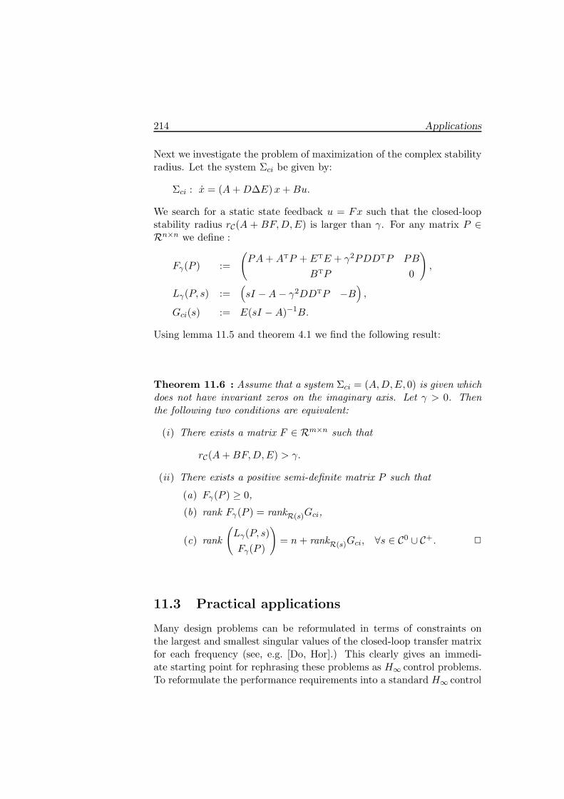
214 Applications
Next we investigate the problem of maximization of the complex stabilityradius. Let the system Σci be given by:
Σci : x = (A+D∆E)x+Bu.
We search for a static state feedback u = Fx such that the closed-loopstability radius rC(A + BF,D,E) is larger than γ. For any matrix P ∈Rn×n we define :
Fγ(P ) :=
(PA+ATP + ETE + γ2PDDTP PB
BTP 0
),
Lγ(P, s) :=(sI −A− γ2DDTP −B
),
Gci(s) := E(sI −A)−1B.
Using lemma 11.5 and theorem 4.1 we find the following result:
Theorem 11.6 : Assume that a system Σci = (A,D,E, 0) is given whichdoes not have invariant zeros on the imaginary axis. Let γ > 0. Thenthe following two conditions are equivalent:
(i) There exists a matrix F ∈ Rm×n such that
rC(A+BF,D,E) > γ.
(ii) There exists a positive semi-definite matrix P such that
(a) Fγ(P ) ≥ 0,
(b) rank Fγ(P ) = rankR(s)Gci,
(c) rank
(Lγ(P, s)Fγ(P )
)= n+ rankR(s)Gci, ∀s ∈ C0 ∪ C+. ✷
11.3 Practical applications
Many design problems can be reformulated in terms of constraints onthe largest and smallest singular values of the closed-loop transfer matrixfor each frequency (see, e.g. [Do, Hor].) This clearly gives an immedi-ate starting point for rephrasing these problems as H∞ control problems.To reformulate the performance requirements into a standard H∞ control

11.3 Practical applications 215
problem, as we are studying in this book, requires the choice of appropri-ate weights. Certainly for multiple-input/multiple-output (MIMO) sys-tems this is not straightforward.
Basically the above translation step is easy for single-input/single-output (SISO) systems where we can use the graphical tools like Bode-and Nyquist diagrams; this is not possible for MIMO systems. Moreover,directional information might be important for the performance criteriaand is clearly lost when using singular values as performance criteria. Thisrequires MIMO weights which translate directional information in termsof singular values. The above should clarify why practical problems arenot solved as soon as you have read this book. A good understanding ofdesign trade-offs (as discussed in, e.g. [FL]) and your system are requiredto construct weights which yield an H∞ control problem which suitablyreflects all your criteria.
Several examples have been treated in literature. These are physicalexamples and reflect what you can and cannot do with H∞ control.
• An aircraft autopilot design: see [SLH, SC]
• Vertical plane dynamics of an aircraft: see [MF, M]
• Large space structure: see [SC2]
• Attitude control of a flexible space platform: see [MF]
• Gas turbine control: see [BW]
• Control design for a 90 MW coal fired fluidized bed boiler: see [Cr].
Basically the above examples discuss the choice of weights, after whichthey simply apply the results as discussed in this book. The only differ-ence is the book [MF]. These authors discuss a design method combiningloop-shaping with robustness requirements. The method is still relativelyad-hoc and needs a more thorough foundation before guaranteeing thekind of problems for which the method can be used.
One major class of problems in design is related to robustness, whichcan be treated by H∞ control via the small gain theorem. However, forreal parameter variations and structured uncertainty the small gain the-orem is very conservative. On the other hand, for high frequency uncer-tainty, like bending modes and, in general, discarded dynamics, the theoryyields very good results. These problems are discussed more specificallyvia the example of the inverted pendulum in the next section.
Up to to this moment we can, in general, only guarantee the existenceof controllers with McMillan degree equal to the sum of the McMillan de-grees of the plant and all the weights. This implies that complex weights

216 Applications
yield high-order controllers. However, in practice we would like to knowwhether a controller of lower McMillan degree exists which still givesan acceptable closed-loop performance. A main area of research, there-fore, lies in reduced order H∞ controllers and in model reduction with anH∞ criterion (see [BH, HB, Mu2]).
A possible theoretical extension of the theory given in this book canbe used to incorporate some specific performance constraints:
• Steady state disturbance rejection: the requirement that theclosed-loop transfer matrix is zero in zero.
• High gain roll-off: the requirement that the closed-loop transfermatrix is strictly proper (or, in general that the k’th (k ≥ 0) deriva-tive of G is strictly proper to guarantee a sufficiently fast roll-off.
These kind of conditions are all based on the requirement that the closed-loop transfer matrix satisfies certain constraints on the imaginary axis.Without proof we shall give the following result. This result stems basi-cally from [HSK] and [Vi, lemma 6.5.9].
Theorem 11.7 : Let a system of the form (2.1) be given. Assume thata compensator of the form (2.4) which is internally stabilizing exists suchthat the closed-loop system has H∞ norm less than one. Moreover, assumethat for si ∈ C0 with i = 1, 2, . . . , j a static controller Ki exists such thatthe resulting closed-loop transfer matrix Gi satisfies Gi(si) = 0. In thiscase there is a time-invariant compensator ΣF of the form (2.4) andwith MacMillan degree less than n + j such that the closed-loop systemis internally stable, the closed-loop transfer matrix Gcl has H∞ norm lessthan one and Gcl(si) = 0 for i = 1, 2, . . . , j. ✷
In the previous theorem si = ∞ is allowed but in this case we shouldreplace Gcl(si) by the corresponding direct-feedthrough matrix of Gcl.Also, if we want the first k derivatives of G to be 0 then this can beincorporated but it will yield an increase of k in the McMillan degree ofthe controller.
Basically these requirements can also be incorporated via weights.However, results like this facilitate the construction of weights. Specificperformance criteria like the ones above can be left out while constructingweights and can be incorporated at a later stage.
Finally it should be noted that there are now several toolboxes avail-able (see, e.g. [CS, Va]) using the software package Matlab which contain

11.4 An inverted pendulum on a cart 217
built-in tools to design controllers based on LQG and H∞ control tech-niques. Singular systems cannot be treated with these toolboxes butsoftware is being developed also using Matlab (see [SE]).
11.4 A design example: an inverted pendulum
on a cart
We shall consider the following physical example of an inverted pendulumon a cart:
✡✡
✡✡✡✡
M❤ ❤
�
✲
✟
✲
ϕ
m
l
u
d
We assume the mass of the pendulum to be concentrated in the top withmass m. l is the length of the pendulum and M is the mass of the cart.To describe the position, d and ϕ express the distance of the cart fromsome reference point and the angle of the pendulum with respect to thevertical axis. The input u is the horizontal force applied to the cart. Allmotions are assumed to be in the plane. We assume that the systemis completely stiff and the friction between the cart and the ground hasfriction coefficient F . Finally let g denote the accelaration of gravity. Wethen have the following non-linear model for this system:
(M +m)d+mlϕ cosϕ−ml(ϕ)2 sinϕ+ F d = u
lϕ− g sinϕ+ dcosϕ = 0
If l �= 0 and M �= 0, then linearization around ϕ = 0 yields the followinglinear model:
d
d
ϕ
ϕ
=
0 1 0 00 − F
M −mgM 0
0 0 0 10 F
lMg(m+M)
lM 0
d
d
ϕ
ϕ
+
01M
0− 1
lM
u
Denote these matrices by A and B respectively. Since g �= 0 our linearizedsystem is always controllable. Assuming our measurements are d and d
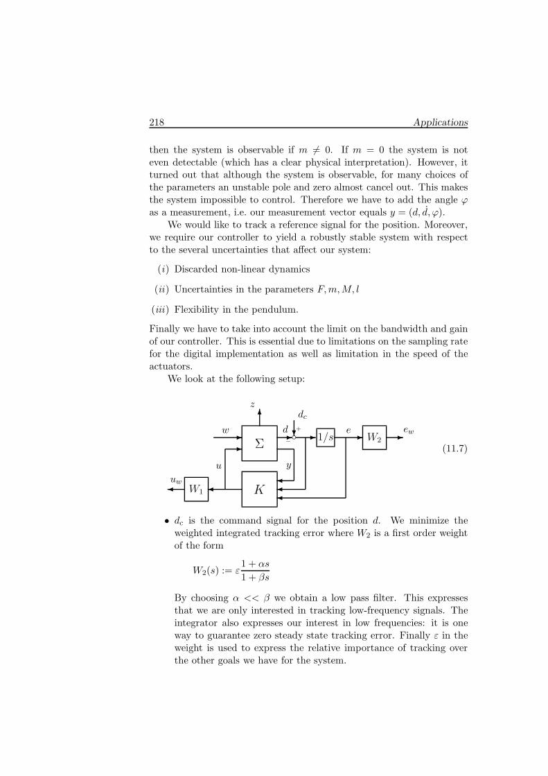
218 Applications
then the system is observable if m �= 0. If m = 0 the system is noteven detectable (which has a clear physical interpretation). However, itturned out that although the system is observable, for many choices ofthe parameters an unstable pole and zero almost cancel out. This makesthe system impossible to control. Therefore we have to add the angle ϕas a measurement, i.e. our measurement vector equals y = (d, d, ϕ).
We would like to track a reference signal for the position. Moreover,we require our controller to yield a robustly stable system with respectto the several uncertainties that affect our system:
(i) Discarded non-linear dynamics
(ii) Uncertainties in the parameters F,m,M, l
(iii) Flexibility in the pendulum.
Finally we have to take into account the limit on the bandwidth and gainof our controller. This is essential due to limitations on the sampling ratefor the digital implementation as well as limitation in the speed of theactuators.
We look at the following setup:
W1 K
Σ1/s W2
✛ ✛
✲✲
✻
✲
✛✛✛
❄ ✲ ✲✲
uw
w
z
d
dc
e
u y
ew◦−
+
(11.7)
• dc is the command signal for the position d. We minimize theweighted integrated tracking error where W2 is a first order weightof the form
W2(s) := ε1 + αs1 + βs
By choosing α << β we obtain a low pass filter. This expressesthat we are only interested in tracking low-frequency signals. Theintegrator also expresses our interest in low frequencies: it is oneway to guarantee zero steady state tracking error. Finally ε in theweight is used to express the relative importance of tracking overthe other goals we have for the system.

11.4 An inverted pendulum on a cart 219
• We also minimize uw which is the weighted control input. W1 hasthe same structure as W2. However, this time we choose α >> β toobtain a high pass filter. We would like to constrain the open-loopbandwidth and gain of the controller. This facilitates digital im-plementation and it also prevents us pushing our actuators beyondtheir capabilities. Finally, it prevents the controller stimulatinghigh-frequency uncertainty in the system dynamics, such as bend-ing modes of the pendulum. Since we cannot incorporate open-looplimitations directly in an H∞ design, we push the bandwidth andgain down indirectly via this weight on u. However, it turned outto be very hard to make the bandwidth small.
• z and w are new inputs and outputs we add to the system Σ toexpress robustness requirements, i.e. the system Σ is of the form:
Σ :
x = Ax + Bu + Ew,
y =
1 0 0 00 1 0 00 0 1 0
x,
z = C2x.
(11.8)
The matrices A and B are as defined before. On the other handE and C2 still have to be chosen. We shall use the technique ofcomplex stability radii described in subsection 11.2.3. For instanceif we want to guard against fluctuations in the parameters F andm, the friction and the mass of the pendulum, then we choose Eand C2 as:
E :=
0−1/M
01/lM
, C2 :=
(0 1 0 00 0 g 0
). (11.9)
A similar definition can be made to guard against fluctuations inall parameters of the 2 differential equations due to discarded non-linearities or flexibility of the beam. The latter are dynamic un-certainties. It should be noted that the complex stability radiusmight be conservative with respect to (real) parameter fluctuations.On the other hand, for discarded dynamics or non-linearities thecomplex stability radius is not conservative. We decided to guard

220 Applications
against all fluctuations in the two differential equations. That is,instead of (11.9), we choose E and C2 as:
E :=
0 01 00 00 1
, C2 :=
1 0 0 00 1 0 00 0 1 00 0 0 1
. (11.10)
On the basis of the above we start designing a controller K for the in-terconnection (11.7) to minimize the H∞ norm from (w, dc) to (z, uw, ew)where we manipulated, by hand, the parameters of the weights W1 andW2 on the basis of the properties of the controllers. It turned out thatthe system Σ is in general much more sensitive to perturbations in allparameters of the differential equation then to perturbations in the pa-rameters F and m. Therefore we incorporate in our design robustnessagainst all parameters of the differential equation. In other words Σ isgiven by (11.8) where E and C2 are given by (11.10).
We would like to stress that optimal controllers have a tendency ofruining every nice property of the system which is not explicitly takeninto account. Our design incorporated a γ iteration. However, we im-plemented the minimum-entropy controller discussed in chapter 7 for a γapproximately 10% larger than the infimum over all stabilizing controllersof the closed-loop H∞ norm. It is our experience that this reduces thebandwidth of the resulting controllers.
We shall give some facts illustrated by frequency and time-responsesof our controller and the resulting closed-loop system. We choose M =1,m = .1, l = 1 and F = 0.1.
(i) The open-loop transfer matrix from u to x and from u to φ aregiven by
Gxu(s) :=(s + 3.13)(s − 3.13)
(s + 3.29)(s − 3.28)(s + 0.09)
Gφu(s) :=−s2
(s + 3.29)(s − 3.28)(s + 0.09)
Hence, it is immediate that because of the near pole-zero cancella-tion in the right half plane that we really need a measurement ofthe angle φ.
(ii) Although not for every choice of the parameters, our final controller,whose Bode magnitude diagram is depicted in figure 11.1, is stable.

11.4 An inverted pendulum on a cart 221
At this moment this desirable property cannot, however, be incor-porated in our design criteria. We obtained a stable controller byplaying around with the parameters. The eigenvalues of the con-troller are −45.7,−22.8,−4.04,−2.37,−1.3±0.51i and −0.667. Thefact that the controller has both very fast and relatively slow modessuggests that via singular perturbation theory (see, e.g. [OM]) wecan reduce the order of the controller. There is, however, no theoryavailable for such an approach.
(iii) Our final controller can, according to the theory developed in sub-section 11.2.3, stand fluctuations in the parameters F and m of400%. Moreover, fluctuations in the parameters of the differentialequations of size less than 0.025 are allowed. The latter is not verymuch but since most parameters are 0 they are in general quitesensitive to fluctuations. Without taking robustness into accountthe final controller could only stand fluctuations of size less than0.000025. Some simulations suggested good robustness properties.
(iv) The time-responses as given in figures 11.5, 11.6 and 11.7 show littleovershoot and therefore the controller is expected to work well onthe non-linear model.
(v) The final controller still has quite a large gain and bandwidth ascan be seen from figure 11.1. The gain is for a large part due to thefact that the controller is translating angles in radians into forcesin Newtons. In general the angles are much smaller than the forces,which is to be expected. The large bandwidth is needed to be ableto stand sudden fluctuations in the angles. The bandwidth andgain of the transfer matrix from dc to u is much smaller as shown infigure 11.3. This transfer matrix is weighted more strongly in ourcost criterion than the effect of fluctuations in φ (since the angle isnot steered directly via a command signal).
(vi) Figure 11.2 shows that we have good tracking properties of low-frequency command signals as required. Tracking can be improvedto 1 rad/sec. However, this results in a controller of much largerbandwidth and gain.
(vii) The loop gain if we break the loop at the control input is given infigure 11.4. The surprising part here is the cross-over angle whichis very small. The angle of the Bode diagram at the cross-overfrequency is related to the phase margin. The fact that this angleis very small suggests a good phase margin.

222 Applications
-80
-60
-40
-20
0
20
40
10-2 10-1 100 101 102 103 104
Frequency- rad/sec
Sing
ular
Val
ue-
dB
Figure 11.1: open loop magnitude Bode diagram of the controller
-250
-200
-150
-100
-50
0
50
10-3 10-2 10-1 100 101 102 103
Frequency- rad/sec
Sing
ular
Val
ue-
dB
Figure 11.2: magnitude Bode diagram from dc to d

11.4 An inverted pendulum on a cart 223
-140
-120
-100
-80
-60
-40
-20
0
10-2 10-1 100 101 102 103 104
Frequency- rad/sec
Sing
ular
Val
ue-
dB
Figure 11.3: magnitude Bode diagram from dc to u
-200
-150
-100
-50
0
50
100
10-2 10-1 100 101 102 103 104
Frequency- rad/sec
Sing
ular
Val
ue-
dB
Figure 11.4: magnitude Bode diagram of the loop gain from uc to u

224 Applications
-0.2
0
0.2
0.4
0.6
0.8
1
1.2
0 5 10 15 20
Time - sec
Posi
tion-
m
-10
-5
0
5
10
15x10-3
0 5 10 15 20
Time - sec
Ang
le-
rad
Figure 11.5: step response from dc to d and φ
-1
-0.8
-0.6
-0.4
-0.2
0
0.2
0.4
0.6
0 5 10 15 20
Time - sec
Posi
tion-
m
-0.08
-0.06
-0.04
-0.02
0
0.02
0.04
0.06
0 5 10 15 20
Time - sec
Ang
le -
rad
Figure 11.6: impulse response from dc to d and φ

11.4 An inverted pendulum on a cart 225
-1
-0.8
-0.6
-0.4
-0.2
0
0.2
0.4
0.6
0 5 10 15 20
Time - sec
Posi
tion-
m
-0.08
-0.06
-0.04
-0.02
0
0.02
0.04
0.06
0 5 10 15 20
Time - sec
Ang
le -
rad
Figure 11.7: impulse response from φ to d and φ
To conclude, we would like to note that we can design controllers viaH∞ control similar as one used to do it via LQG control. However, itis our belief that the H∞ norm makes it easier and more transparentto incorporate several performance requirements in our cost criterion,especially those performance requirements which are directly related torobustness and magnitude Bode diagrams. However a lot of work stillneeds to be done. In particular we have to gain experience similar to thatwe have gained for LQG to translate our criteria into a well-formulatedH∞ problem.

Chapter 12
Conclusion
In this book we have derived several results concerning the H∞ controlproblem. Naturally the research in this area is not completed by thisbook and several interesting open problems remain. In this chapter wefirst devote a section to a discussion of the main contributions of this bookto the active research area of H∞ control. In section 12.2, we discuss someopen problems which could be of interest for future research. Then, inthe last section, we give our final concluding remarks on this book.
12.1 Summary of results obtained
The results derived in this book are related to a number of research areaswithin the framework of H∞ control:
• Singular systems
• Differential games
• Finite horizon H∞ control problem
• Minimum entropy H∞ control problem
• H∞ control for discrete time systems.
We shall briefly discuss our contributions to these five subjects.
12.1.1 Singular systems
For systems which are not necessarily regular, we derived necessary andsufficient conditions for the existence of an internally stabilizing controllerwhich makes the H∞ norm strictly less than some, a priori given, numberγ. For the measurement-feedback case these conditions are in terms of
226

12.1 Summary of results obtained 227
solutions of two quadratic matrix inequalities and four associated rankconditions. This can be shown to be equivalent to the existence of twostabilizing solutions of reduced order Riccati equations.
In our opinion, our proof yields a nice understanding of the structureof the H∞ control problem. However, our algorithm for finding a suitablecontroller, if one exists, is still not completely satisfactory.
At this point we shall outline the main steps of the proof of theorem5.1, which is our main result for singular systems. This is done becausethe main steps give nice insight in the structure of theH∞ control problemas we see it.
We start with a system of the form (5.1). We first investigate how wellwe can regulate the system if we have all information of the state and thedisturbance available. We can derive necessary and sufficient conditionsunder which we can find a controller which makes the H∞ norm less thansome bound γ (a so-called suitable controller), by investigating a sup-infproblem:
supw
infu
{‖zu,w,ξ‖22 − γ2‖w‖22 | u ∈ Lm2 , w ∈ Ll2 such that xu,w,ξ ∈ Ln2
}
(12.1)
for arbitrary initial state x(0) = ξ. We solved this problem using ideassupplied by Pontryagin’s Maximum Principle. We did this explicitly forregular systems and we extended it to general systems by some decom-positions of the state space, the input space and the output space (thatthis extension to the general case is related to the same sup-inf problemcan be seen more easily by investigating the results of chapter 6). Wefind necessary and sufficient conditions under which a suitable controllerexists: there should be a positive semi-definite solution to a quadraticmatrix inequality which satisfies two rank conditions. This can be shownto be equivalent to the existence of a stabilizing solution to an algebraicRiccati equation (a reduced order Riccati equation if the system is sin-gular). Although our proof might not be the most simple one available ithas one clear advantage. It shows that we cannot do better with respectto minimizing the H∞ norm by allowing more general (e.g. non-linear ornon-causal) controllers.
We now return to the general case where we might have only partialinformation on the state and the disturbance. If a suitable controller withmeasurement feedback exists, then there is certainly a suitable controllerfor the full-information feedback case. Hence, there is a positive semi-definite solution to our quadratic matrix inequality and the correspondingrank conditions. Then we can transform our original system Σ into a new

228 Conclusion
system ΣP . A controller is suitable for Σ if, and only if, a controller issuitable for ΣP (this is true for controllers with measurement feedbackand for controllers with state feedback). However this new system ΣP
has the interesting property that we can find state feedbacks which areinternally stabilizing and which make the H∞ norm of the closed-loopsystem arbitrarily small (ADDPS, as discussed in section 2.6, is solvable).
The problem of whether we can measure the state well enough to finda suitable controller with measurement feedback still remains. It turnsout that this problem is exactly dual to the problem of full-informationH∞ control: minimizing the induced norm from w to z for some sys-tem Σt by full-information feedback is essentially the same problem asbuilding an observer for the state of ΣT
t which minimizes the inducednorm of the operator from w to x − x where x denotes the estimatedstate. Hence, we immediately find necessary and sufficient conditions un-der which we can observe the state of ΣP well enough: there should bea positive semi-definite solution to a second quadratic matrix inequalitywhich has to satisfy two rank conditions (remember that we already hada solution to one quadratic matrix inequality before our transformationfrom Σ to ΣP ). Thus we obtain a necessary condition for the existenceof a suitable controller: we should have solutions of two quadratic matrixinequalities and four corresponding rank conditions. These conditions arealso sufficient. To show this we apply a second transformation, dual tothe first, from ΣP to ΣP,Q. Again, a controller is suitable for ΣP if, andonly if, this controller is suitable for ΣP,Q. For ΣP,Q we can observe thestate arbitrarily well. Surprisingly enough ΣP,Q still has the same niceproperty ΣP has: there is an internally stabilizing state feedback whichmakes the H∞ norm of the closed-loop system arbitrarily small (ADDPSis solvable). This implies that we can find a controller with measurementfeedback which is internally stabilizing and which makes the H∞ norm ofthe closed-loop system associated with ΣP,Q arbitrarily small (ADDPMSis solvable). We can make the H∞ norm of the closed-loop system equalto 0 if the system Σ is regular (DDPMS is solvable), but we cannot dothis in general.
The conditions we thus obtained can be reformulated to yield theconditions of theorem 5.1. The problem is that our second quadraticmatrix inequality as defined above is in terms of the system ΣP . Rewritingthis second matrix inequality with two corresponding rank conditions interms of Σ yields one quadratic matrix inequality, two rank conditionsand a coupling condition.

12.1 Summary of results obtained 229
12.1.2 Differential games
Differential games are not worked out in much detail in this book. How-ever, some of the results obtained yield nice intuition.
Firstly we note that the quadratic form associated with the solution ofour quadratic matrix inequality yields an almost Nash equilibrium whilefor the regular problem we obtain an (exact) Nash equilibrium.
Moreover, as we noted in the previous subsection, the results forthe regular state feedback H∞ control problem were derived by investi-gating a sup-inf problem (12.1). The value of (12.1) is, as a functionof ξ, equal to the quadratic form given by the solution of the algebraicRiccati equation. The general full-information H∞ control problem withstate feedback was solved by reducing the general problem to the regularH∞ control problem. In chapter 6, while discussing differential games, wefind as a side result that the quadratic form associated with the solutionof the quadratic matrix inequality again yields the value of (12.1) as afunction of ξ. This is a nice result to complete the picture we have of theH∞ control problem.
Another interesting fact is that a necessary condition for the existenceof an almost equilibrium is the possibility of making the H∞ norm lessthan or equal to 1 and a sufficient condition is the possibility of makingthe H∞ norm strictly less than 1. All of this holds under the constraintof internal stability and with state feedback. This provides a naturalstarting point for research for testing whether we can make the H∞ normless than or equal to 1, as done in [Gl6] for the regular case.
12.1.3 The minimum entropy H∞ control problem
In chapter 7 we discuss the minimum entropy H∞ control problem. Weonly discussed a very limited case. In the general setup of subsection 1.6.3we only discuss the case that we have one closed-loop transfer matrixon which we want to satisfy an H∞ norm bound while minimizing theH2 norm of this same transfer matrix. Not even that, we used only anupper bound for the LQG cost criterion. This problem therefore appearsin one of the coming sections as one of the major open problems.
What did we do? By restraining attention to “entropy at infinity” wecould make the proofs of [Mu] more straightforward and less technical.Moreover, we showed how you could extend this result to singular systems.This chapter is meant to be a starting point for future research in thisarea. In our opinion this chapter sketches ideas which could also beapplied to the more general case of subsection 1.6.3.

230 Conclusion
12.1.4 The finite horizon H∞ control problem
In chapter 8 we discussed the L2[0, T ]-induced operator norm insteadof the usual H∞ norm which is equal to the L2[0,∞)-induced operatornorm. We derived conditions under which we could find a time-varyingcontroller which makes the L2[0, T ]-induced operator norm less than somea priori given number γ > 0. Instead of a Riccati differential equation weobtain, for singular systems, a quadratic differential inequality togetherwith a number of rank conditions. Solvability of this quadratic differentialinequality can be tested by using the basis of appendix A. It turns outto be equivalent to a reduced-order Riccati differential equation.
For regular systems the techniques used can equally well be appliedto time-varying systems. This is not true for singular systems. Our proofsare strongly based on the bases of appendix A and we have to make anumber of assumptions to make sure these bases are not time-varying.This is not worked out in detail in this book but can be found in [St7].
12.1.5 Discrete time systems
For discrete time systems which are discrete time analogues of regularcontinuous time systems, we were able to derive nice conditions: a suitablecontroller exists if, and only if, there are positive semi-definite stabilizingsolutions to two algebraic Riccati equations. This certainly shows thattransformations to the continuous time case are not necessary and thatH∞ control can be applied directly to discrete time systems. However,we should spend some time on deriving numerically reliable methods tocheck whether these Riccati equations indeed have solutions or not and,if they exist, to calculate the solutions.
The techniques used to derive this result were completely similar tothe techniques we used to derive the results for the regular continuoustime H∞ control problem. However, for discrete time systems there area number of extra technicalities and the formulae are rather complexand cumbersome. On the other hand, there is one essential difference:for continuous time systems we could do no better by allowing for non-causal feedbacks. This is not true for discrete time systems: it is possibleto attain H∞ norms of the closed-loop system via non-causal controllerswhich cannot be attained nor approximated by causal controllers.
12.2 Open problems
We shall mention some problems of interest in the next two subsections.Clearly this list is not exhaustive and several other open problems remain.

12.2 Open problems 231
12.2.1 Invariant zeros
Throughout this book, we have excluded invariant zeros on the imaginaryaxis for continuous time systems. For discrete time systems, invariantzeros on the unit disc have been excluded. In this subsection we wantto discuss the difficulty of these invariant zeros intuitively. The readershould not expect formal proofs in this section.
A treatment of invariant zeros on the imaginary axis for continuoustime systems is given in several papers, [HSK, S3, S4]. For the regularstate feedback case (no problems at infinity) the conditions in [S3] can, inprinciple, be reformulated as: a solution of a Riccati equation exists forwhich the matrix Acl as given in theorem 3.1 has all eigenvalues in theopen left half plane or in points on the imaginary axis which are invariantzeros. Besides that, separate extra conditions have to be satisfied for eachinvariant zero on the imaginary axis.
However, it is worthwhile to look for alternative formulations of theresults in [HSK, S3, S4] in order to obtain a better insight of what theextra conditions which have to be satisfied when we have an invariantzero on the imaginary axis look like.
Moreover, a numerical reliable way of finding a suitable controller, ifone exists, is needed. As in this book, in [S3, S4] a geometric approachis chosen. This yields good understanding of the nature of the problemsbut gives results which are in general numerically not very reliable.
Next, we shall try to show the difficulty of invariant zeros on theimaginary axis for continuous time systems. Our approach is based onthe paper [HSK], which only treats the regular one block problem (D12
and D21 in (2.1) are both square invertible matrices).The H∞ control problem with measurement feedback can be reduced
to the so-called model-matching problem (see [Fr2]). This is the followingproblem:
infQ∈H∞
‖T1 − T2QT3‖∞, (12.2)
where T1, T2 and T3 are given matrices in H∞ . For the sole reason ofan easy exposition of the problems we assume that T2 and T3 are, asrational matrices, right- and left-invertible, respectively. In this case forQ1 := T+
2 T1T+3 (+ denotes a right cq. left inverse) we have
T1 − T2Q1T3 = 0.
However, in general, Q1 will not be in H∞ . The invariant zeros of thetwo subsystems (A,B,C2,D2) and (A,E,C1,D1) (using the definitions oftheorem 5.1) are the only points in the complex plane where T2 and T3,

232 Conclusion
respectively, might have a zero, i.e. lose rank. The right cq. left inversewill then have a pole in these points. Hence if we have only invariantzeros in the open left half plane, then Q1 will be in H∞ .
Invariant zeros in the open left half plane do not give rise to con-straints on the attainable closed-loop system T1 − T2QT3. On the otherhand, invariant zeros in the open right half plane do yield constraintson the attainable closed-loop system. A zero on the imaginary axis can,however, be cancelled approximately by choosing Q such that it has apole in the left half plane arbitrarily close to the zero on the imaginaryaxis. It turns out that for these points the only constraint is a conditionin terms of the transfer matrices evaluated in this point itself. If we haveonly invariant zeros on the imaginary axis we find the constraint thatthe infimum in (12.2) is less than 1 if, and only if, for all invariant zeross ∈ C0 a constant matrix Ks exists such that
‖T1(s)− T2(s)KsT3(s)‖ < 1.
For invariant zeros in the open right half plane this condition is necessarybut not sufficient for the infimum to be less than 1.
This shows that zeros on the imaginary axis and zeros in the righthalf plane need a different approach and that is exactly the difficulty wehave in treating the most general case with both invariant zeros on theimaginary axis as well as zeros in the open right half plane.
We expect that for the general case without assumptions on the sys-tem and with continuous time, we can find the following necessary andsufficient conditions for the existence of a suitable controller (we shall usethe notation as was already used in theorem 5.1): we think that the exis-tence of matrices P and Q which satisfy the quadratic matrix inequalitiesFγ(P ) ≥ 0 and Gγ(Q) ≥ 0 and which satisfy the rank conditions (a) and(b) of theorem 5.1 are conditions which are always needed.
For any s in the closed right half plane which is not an invariant zeroof either (A,B,C2,D2) or (A,E,C1,D1), rank conditions (c) or (d) oftheorem 5.1 should still be satisfied.
The condition for invariant zeros of (A,B,C2,D2) or (A,E,C1,D1)in the open right half plane is that rank conditions (c) and (d) of theorem5.1 should still be satisfied. However, for invariant zeros of (A,B,C2,D2)or (A,E,C1,D1) on the imaginary axis the rank conditions (c) and (d)should be replaced by some weaker condition.
12.2.2 Mixed H∞ /. . . problems
As we already noted in section 1.1 robustness plays a key role in controltheory. In this book we investigated H∞ control problems which play an

12.3 Conclusion of this book 233
essential role in robustness of internal stability as outlined in section 11.2.However, it often happens that we are not only interested in robustness ofinternal stability but in robustness analysis of other preformance criteriaas well.
Mixed Linear Quadratic Gaussian (LQG) and H∞ control problemsas introduced in subsection 1.6.3 are quite well suited for the above ob-jective. We made a start with the discussion of this problem in chapter7. For regular systems a quite extensive literature is already available(see section 7.1). However all these papers discuss an entropy functioninstead of the LQG criterion. The real mixed LQG/H∞ control problemis still completely unsolved.
There are also other kinds of mixed problems which are of interestbut which have not received much attention. For instance, in the aboveproblems the sensitivity of the LQG criterion to system perturbations isnot incorporated in the controller design. Only the sensitivity of internalstability to system perturbations is taken into account. The main problemof course remains the trade-off between robustness and performance. Thisalso yields problems with respect to the required model accuracy andbounds on the McMillan degree of the controller.
12.3 Conclusion of this book
In this book we have generalized existing theorems on the standard H∞control problem. Interesting open problems at this moment are more spe-cific applications of H∞ control which are non-standard, e.g. the above-mentioned mixed problems. The main open problem at this moment isrelated to the practical application of H∞ control. Although we feel thatthe theoretical H∞ control problem and its structure are well understoodat the moment, the practical issue of the design of weights for multi-input, multi-output systems lacks a systematic approach. Besides that,theH∞ control problems with either invariant zeros on the imaginary axis(unit disc for discrete time systems) or with problems at infinity are nowreasonably well understood but they need numerically more reliable al-gorithms to check existence of suitable controllers and to calculate them,if they exist.
We feel that this book and the large number of papers mentioned inthe references give a very thorough basic understanding of the H∞ controlproblem. Nevertheless the subject will remain an important research areain the near future. This is due to the fact that we still need to makethe step from basic understanding to design (how to apply all this nicetheory in practice). Moreover, because of the extreme importance of

234 Conclusion
robustness and its strong correlation with H∞ , its relation with almostall aspects of system and control theory is interesting. We could thinkof identification with H∞ error bounds (see, e.g. [HJN, GK, GK2]) andother combinations which at the moment might be far-fetched. However,control engineers working in practice will be the first to acknowledge thatthe main reason why they are sceptical about applying modern controlschemes is their concern about robustness. They sometimes even claimthat all modern schemes including controllers built with H∞ performancecriteria are not robust and only classical P(I)(D) controllers can be trustedto control their expensive machinery. The control engineer in practiceshould realize that, although we present this new tool of H∞ control ina very mathematical setting, in fact H∞ control is nothing other thenapplying the available theoretical machinery to the problem of obtainingthe desired shape of the closed-loop Bode diagram.
It is our belief that in the future H∞ will lead to robust and reliablecontrollers but a lot of work has to be done in order to be ready totackle real-life control problems (which will often be MIMO systems) ina structured and reliable way.

Appendix A
Preliminary basis transformations
A.1 A suitable choice of bases
In this section we shall choose bases to identify for systems (A,B,C,D)with D not injective, a regular subsystem which contains all essentialfeatures of the H∞ control problem. We start by applying a suitable statefeedback transformation u = F0x + v to the system Σci = (A,B,C,D).It is transformed into a system Σci,F0 := (A+BF0, B,C +DF0,D) witha very particular structure. We shall display this structure by writingdown the matrices of the mappings A+BF0, B,C +DF0,D with respectto suitable bases in the input spaceRm, the state spaceRn and the outputspace Rp. In this section we shall use the notation AF0 := A+BF0 andCF0 := C +DF0 .
Our basic tool is the strongly controllable subspace. This subspacehas been defined and some of its properties have been given in section2.4. We now define the bases which will be used in the sequel.
First choose a basis of the input spaceRm as follows. Let u1, u2, . . . , umbe a basis such that u1, u2, . . . , ui is a basis of kerD (0 ≤ i ≤ m). In otherwords, decompose Rm = U1 ⊕U2 such that U2 = kerD and U1 arbitrary.Next, choose a basis of the output space Rp as follows. Let z1, z2, . . . , zpbe an orthonormal basis such that z1, . . . , zj is an orthonormal basis ofimD and zj+1, . . . , zp is an orthonormal basis of (im D)⊥. (0 ≤ j ≤ p).In other words, write Rp = Z1 ⊕Z2 with Z1 = imD and Z2 = (im D)⊥.Because this is an orthonormal basis this basis transformation does notchange the norm ‖z‖.
235
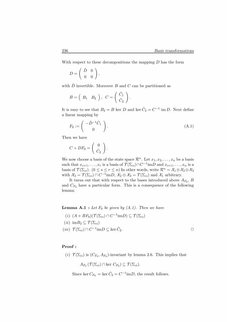
236 Basis transformations
With respect to these decompositions the mapping D has the form
D =
(D 00 0
),
with D invertible. Moreover B and C can be partitioned as
B =(B1 B2
), C =
(C1
C2
).
It is easy to see that B2 = B ker D and ker C2 = C−1 imD. Next definea linear mapping by
F0 :=
(−D−1C1
0
). (A.1)
Then we have
C +DF0 =
(0C2
).
We now choose a basis of the state space Rn. Let x1, x2, . . . , xn be a basissuch that xs+1, . . . , xr is a basis of T (Σci)∩C−1imD and xs+1, . . . , xn is abasis of T (Σci). (0 ≤ s ≤ r ≤ n) In other words, write Rn = X1⊕X2⊕X3
with X2 = T (Σci) ∩ C−1imD, X2 ⊕X3 = T (Σci) and X1 arbitrary.It turns out that with respect to the bases introduced above AF0, B
and CF0 have a particular form. This is a consequence of the followinglemma:
Lemma A.1 : Let F0 be given by (A.1). Then we have
(i) (A+BF0)(T (Σci) ∩ C−1imD) ⊆ T (Σci)
(ii) imB2 ⊆ T (Σci)
(iii) T (Σci) ∩ C−1imD ⊆ ker C2. ✷
Proof :
(i) T (Σci) is (CF0, AF0)-invariant by lemma 2.6. This implies that
AF0 (T (Σci) ∩ ker CF0) ⊆ T (Σci).
Since kerCF0 = ker C2 = C−1imD, the result follows.

A.1 A suitable choice of bases 237
(ii) Let Ti(Σci) be the sequence defined by (2.15). Then we know thatT1(Σci) = B ker D = imB2. Since Ti(Σci) is non-decreasing thisproves our claim.
(iii) This follows immediately from the fact that C−1imD = ker C2.
By applying this lemma we find that the matrices A+BF0, B, C +DF0
and D with respect to these bases have the following form.
A+BF0 =
A11 0 A13
A21 A22 A23
A31 A32 A33
, B =
B11 0B21 B22
B31 B32
,
C +DF0 =
(0 0 0C21 0 C23
), D =
(D 00 0
).
(A.2)
We apply the preliminary feedback u = F0x + v to the system Σ, givenby
Σ :
{x = Ax + Bu + Ew,
z = Cx + Du.(A.3)
Denote the resulting system by ΣF0. We decompose x,v and z corre-sponding to the bases in state, input and output space, i.e.
x =
x1
x2
x3
, v =
(v1
v2
), z =
(z1
z2
).
We also decompose E and C1 corresponding to the bases defined:
C1 =(C11 C12 C13
), E =
E1
E2
E3
. (A.4)
Hence we have
C =
(C1
C2
)=
(C11 C12 C13
C21 0 C23
).
In our new bases the system ΣF0 then has the following form:
x1 = A11x1 +(B11 A13
)(v1x3
)+ E1w, (A.5)

238 Basis transformations
(x2
x3
)=
(A22 A23
A32 A33
)(x2
x3
)+
(B22
B32
)v2+
(B21 A21
B31 A31
)(v1
x1
)+
(E2
E3
)w,(A.6)
(z1
z2
)=
(0C21
)x1 +
(D 00 C23
)(v1
x3
). (A.7)
As already suggested by the way in which we arranged these equations,the system ΣF0 can be considered as the interconnection of two subsys-tems. This is depicted in the following diagram:
v2 ✲✲
v1 ✲
Σ0
Σ
❄
✻x1 x3
✲
✲
w ∩
✲
(z1
z2
)
(A.8)
In the picture (A.8), Σ is the system given by the equations (A.5) and(A.7). It has input space U1×X3×Rl, state space X1 and output spaceRp.The system Σ0 is given by equation (A.6). It has input spaceRm×X1×Rl,state space X2⊕X3 and output space X3. The interconnection is made viax1 and x3 as in the diagram. Note that Σ and ΣF0 have the same outputequation. However, in ΣF0 the variable x3 is generated by Σ0 while in Σit is considered as an input and is free.
The systems Σ and Σ0 turn out to have some nice structural proper-ties:
Lemma A.2 :
(i) C23 is injective,
(ii) The system,
Σ1 :=
[(A22 A23
A32 A33
),
(B22
B32
),(0 I
), 0
](A.9)
with input space U2, state space X2 ⊕ X3 (= T (Σci)) and outputspace X3 is strongly controllable. ✷

A.1 A suitable choice of bases 239
Proof :
(i) Let (xT1 , x
T2 , x
T3 )
T be the coordinate vector of a given x ∈ Rn. As-sume that C23x3 = 0. Let x ∈ Rn be the vector with coordinates(0T, 0T, xT
3 ). Then x ∈ X3. In addition, x ∈ T (Σci) ∩ kerC2 = X2.Thus x = 0 so x3 = 0.
(ii) Let T (Σ1) be the strongly controllable subspace of the system Σ1
given by (A.9). We shall prove T (Σ1) = X2 ⊕ X3. First note thatthere exists G :=
(GT
2 GT3
)T
such that
[(A22 A23
A32 A33
)+
(G2
G3
)(0 I
)]T (Σ1) ⊆ T (Σ1).
Also note that
im
(B22
B32
)⊆ T (Σ1).
Now assume that T (Σ1) ⊂ X2 ⊕ X3 with strict inclusion. DefineV ⊆ Rn by
V :=
0x2
x3
(x2
x3
)∈ T (Σ1)
.
Clearly, V ⊂ T (Σci) with strict inclusion. We claim that a linearmap G0 : Rp →Rn exists such that
(A+G0C)V ⊆ V, (A.10)
and
im (B +G0D) ⊆ V. (A.11)
Indeed, let C+23 be any left inverse of C23 and define
G0 :=
B11 −A13
B21 G2
B31 G3
(−D−1 00 C+
23
).
It is then straightforward to check (A.10) and (A.11). This, how-ever, contradicts the fact that T (Σci) is the smallest subspace V forwhich (A.10) and (A.11) hold (see definition 2.3). We conclude thatX2 ⊕X3 = T (Σ1).

240 Basis transformations
Our next result states that the zero structure of Σci = (A,B,C,D) iscompletely determined by the zero structure of Σci defined by
Σci :=
[A11,
(B11 A13
),
(0C21
),
(D 00 C23
)]. (A.12)
Note that Σci is a subsystem of Σ (where Σ is described by (A.5) and(A.7)) in the same way as Σci is a subsystem of Σ (where Σ is describedby (A.3)).
Lemma A.3 : The non-trivial transmission polynomials of Σci and Σci,respectively, coincide. ✷
Proof : According to section 2.3 the transmission polynomials of Σci =(A,B,C,D) and Σci,F0 = (AF0 , B,CF0 ,D) coincide. Thus, in order toprove the lemma, it suffices to show that the system matrix Pci,F0 ofΣci,F0 is unimodularly equivalent to a polynomial matrix of the form
(Pci 0 00 I 0
),
where Pci is the system matrix of Σci. Since Σ1, as defined by (A.9), isstrongly controllable and ( 0 I ) is surjective, by lemma 2.8 the Smith
form of the system matrix P1 of Σ1 is equal to ( I 0 ). In addition weclearly have
P1 ∼
sI −A22 0 −B22
−A22 0 −B32
0 I 0
∼
sI −A22 −B22 0−A22 −B32 00 0 I
,
so we conclude that(sI −A22 −B22
−A22 −B32
),

A.1 A suitable choice of bases 241
is unimodularly equivalent to ( I 0 ). The proof is then completed bynoting that
Pci,F0 ∼
sI −A11 −B11 −A13 0 00 D 0 0 0C21 0 C23 0 0−A21 −B21 −A23 sI −A22 −B22
−A31 −B31 sI −A33 −A32 −B32
∼(Pci 0 00 I 0
).
A consequence of the above lemma is that the invariant zeros of Σci andΣci, respectively, coincide.
Our next lemma states that the normal rank of the transfer matrix
Gci(s) := C(sI −A)−1B +D, (A.13)
of the system Σci is equal to the number (rank D + dim X3) or, equiva-lently,
Lemma A.4 : We have
rankR(s)Gci = rank
(C23 00 D
). ✷
Proof : Define L(s) := sI −A. Then we have
rankR(s)
(L 00 Gci
)= n+ rankR(s)Gci. (A.14)
We also have(L(s) 00 Gci(s)
)∼
(sI −AF0 −BCF0 D
)
=
sI −A11 0 −A13 −B11 0−A21 sI −A22 −A23 −B21 −B22
−A31 −A32 sI −A33 −B31 −B32
0 0 0 D 0C21 0 C23 0 0
.

242 Basis transformations
Since C23 and D are injective we can make the (1,3), (1,4), (2,4) and (3,4)blocks zero by unimodular transformations. Furthermore we make a basistransformation on the output such that C23 has the form ( Ir 0 )T wherer = rank C23. Thus, after suitable permutation of blocks, the normalrank of the latter matrix turns out to be equal to the normal rank of
sI − A11 0 0 0 0
−A21 sI − A22 −A23 −B22 0
−A31 −A32 sI − A33 −B32 0
C211 0 Ir 0 0
C212 0 0 0 0
0 0 0 0 D
.
Here A11 is a given matrix. Since, by lemma 4.2, the matrix in the centrebox has full row rank for all s ∈ C and rankR(s)(sI − A11) = dim X1 wefind
rankR(s)
(L 00 Gci
)= n+ rank
(C23 00 D
).
Combining this with (A.14) gives the desired result.
To conclude we want to note that if D is injective, then the subspace U2
in the decomposition of Rm vanishes. Consequently, the partitioning of Breduces to a single block and the partitioning of D reduces to ( DT 0 )T
with D invertible. It is left as an exercise to the reader to show thatT (Σci) = {0} if, and only if, ker D ⊂ ker B. Thus, if D is injective, thenalso T (Σci) = {0}. In that case the subspaces X2 and X3 appearing inthe decomposition of the state space Rn both vanish and the partitioningof AF0 reduces to a single block.
A.2 The quadratic matrix inequality
We shall now derive some properties for matrices satisfying the quadraticmatrix inequality, i.e. matrices P such that
F (P ) :=
(ATP + PA+ PEETP + CTC CTD + PB
DTC +BTP DTD
)≥ 0.
We first derive a result which is one of the key lemmas of this book.

A.2 The quadratic matrix inequality 243
Lemma A.5 : Assume that a symmetric P is a solution of F (P ) ≥ 0.We have P T (Σci) = 0, i.e in our decomposition P can be written as
P =
P1 0 00 0 00 0 0
. (A.15)
✷
Proof : Let F0 be given by (A.1). Since DTCF0 = 0 (this can be checkedeasily) we may apply lemma 2.7. We define
M(P ) :=
(I FT
0
0 I
)F (P )
(I 0F0 I
). (A.16)
If F (P ) ≥ 0, then also
M(P ) =
(PAF0 +A
TF0P + PEETP + CT
F0CF0 PB
BTP DTD
)≥ 0
We claim B ker D ⊆ ker P . Let u ∈ Rm be such that Du = 0. Then wefind
(0T uT
)M(P )
(0u
)= 0
and hence, since M(P ) ≥ 0, we find
M(P )
(0u
)= 0.
This implies PB = 0. Next we have to show that kerP is (CF0 , AF0)invariant. Assume that x ∈ ker P ∩ ker CF0. Then
xT(PAF0 +A
TF0P + PEETP + CT
F0CF0
)x = 0.
Hence, by applying x to one side only, we find PAF0 = 0 and thereforeAF0x ∈ ker P . Since T (Σci) is the smallest space with these two prop-erties we have T (Σci) ⊆ ker P .
Using the above we can derive the following result. Note that Gci is thetransfer matrix defined by (A.13).

244 Basis transformations
Theorem A.6 : Let P ∈ Rn×n be symmetric. The following two state-ments are equivalent:
(i) P is a symmetric solution to the quadratic matrix inequality, i.e.we have F (P ) ≥ 0. Moreover, rank F (P ) = rankR(s)Gci.
(ii) If P is in the form (A.15) and if we define
R(P1) := P1A11 +AT11P1 + P1
(E1E
T1 − B11
(DTD
)−1
BT11
)P1+
CT21C21 −
(AT
13P1 + CT23C21
)T (CT
23C23
)−1 (AT
13P1 + CT23C21
),
(A.17)
then we have R(P1) = 0.
Let s0 ∈ C be given. If (i) holds (or equivalently (ii)), then the followingstatements are equivalent:
(iii) P satisfies
rank
(L(P, s0)F (P )
)= n+ rankR(s)Gci.
(iv) The matrix Z(P1) defined by
Z(P1) := A11 + E1ET1 P1 −B11
(DTD
)−1BT
11P1
−A13 (CT23C23)
−1 (AT13P1 +CT
23C21) (A.18)
has no eigenvalue in s0. ✷
Proof : By (A.16) we have M(P ) ≥ 0 if, and only if, F (P ) ≥ 0 andwe also know that these matrices have the same rank. Assume that asymmetric P satisfies M(P ) ≥ 0 and rank M(P ) = rankR(s)Gci. Bylemma A.5 we know that in our new basis we can write P in the form(A.15). If we also use the decompositions (A.2) and (A.4) for the othermatrices we find that M(P ) is equal to
P1A11 + AT11P1 + CT
21C21 + P1E1ET1 P1 0 P1A13 + CT
21C23 P1B11 0
0 0 0 0 0
AT13P1 + CT
23C21 0 CT23C23 0 0
BT11P1 0 0 DTD 0
0 0 0 0 0
.
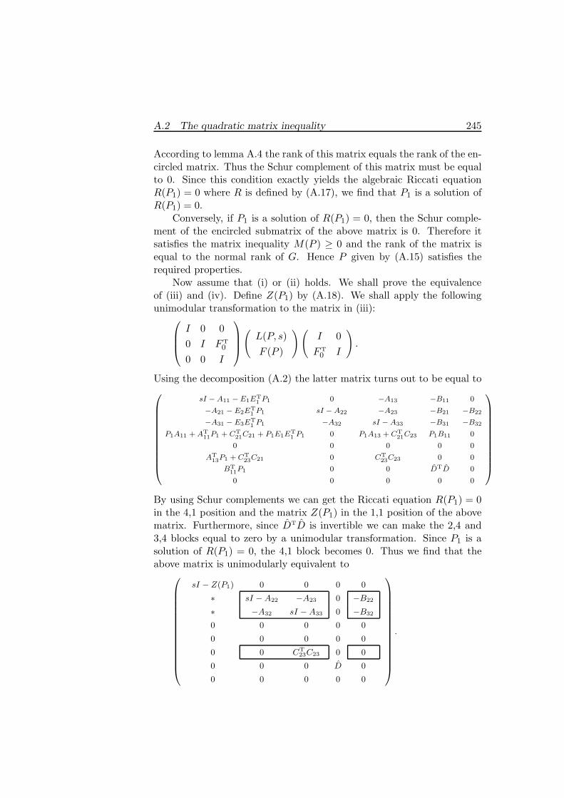
A.2 The quadratic matrix inequality 245
According to lemma A.4 the rank of this matrix equals the rank of the en-circled matrix. Thus the Schur complement of this matrix must be equalto 0. Since this condition exactly yields the algebraic Riccati equationR(P1) = 0 where R is defined by (A.17), we find that P1 is a solution ofR(P1) = 0.
Conversely, if P1 is a solution of R(P1) = 0, then the Schur comple-ment of the encircled submatrix of the above matrix is 0. Therefore itsatisfies the matrix inequality M(P ) ≥ 0 and the rank of the matrix isequal to the normal rank of G. Hence P given by (A.15) satisfies therequired properties.
Now assume that (i) or (ii) holds. We shall prove the equivalenceof (iii) and (iv). Define Z(P1) by (A.18). We shall apply the followingunimodular transformation to the matrix in (iii):
I 0 00 I FT
0
0 0 I
(L(P, s)F (P )
)(I 0FT
0 I
).
Using the decomposition (A.2) the latter matrix turns out to be equal to
sI − A11 − E1ET1 P1 0 −A13 −B11 0
−A21 − E2ET1 P1 sI − A22 −A23 −B21 −B22
−A31 − E3ET1 P1 −A32 sI − A33 −B31 −B32
P1A11 + AT11P1 + CT
21C21 + P1E1ET1 P1 0 P1A13 + CT
21C23 P1B11 0
0 0 0 0 0
AT13P1 + CT
23C21 0 CT23C23 0 0
BT11P1 0 0 DTD 0
0 0 0 0 0
By using Schur complements we can get the Riccati equation R(P1) = 0in the 4,1 position and the matrix Z(P1) in the 1,1 position of the abovematrix. Furthermore, since DTD is invertible we can make the 2,4 and3,4 blocks equal to zero by a unimodular transformation. Since P1 is asolution of R(P1) = 0, the 4,1 block becomes 0. Thus we find that theabove matrix is unimodularly equivalent to
sI − Z(P1) 0 0 0 0
∗ sI − A22 −A23 0 −B22
∗ −A32 sI − A33 0 −B32
0 0 0 0 0
0 0 0 0 0
0 0 CT23C23 0 0
0 0 0 D 0
0 0 0 0 0
.
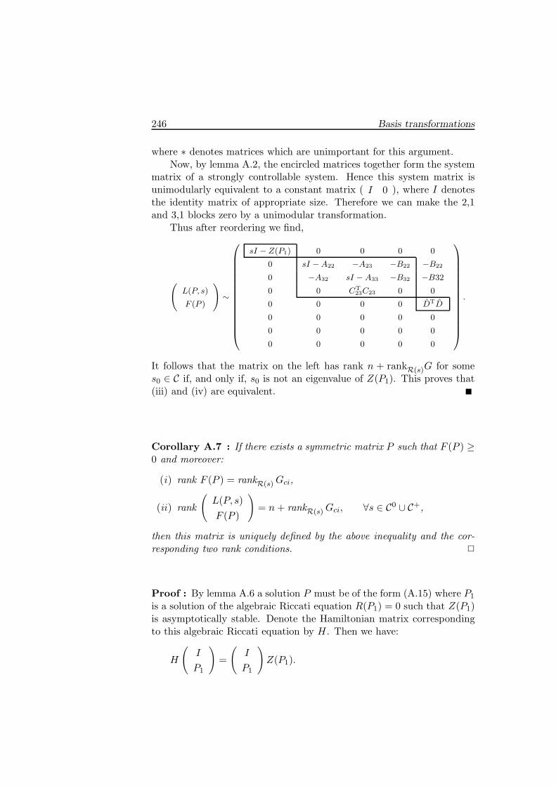
246 Basis transformations
where ∗ denotes matrices which are unimportant for this argument.Now, by lemma A.2, the encircled matrices together form the system
matrix of a strongly controllable system. Hence this system matrix isunimodularly equivalent to a constant matrix ( I 0 ), where I denotesthe identity matrix of appropriate size. Therefore we can make the 2,1and 3,1 blocks zero by a unimodular transformation.
Thus after reordering we find,
(L(P, s)
F (P )
)∼
sI − Z(P1) 0 0 0 0
0 sI − A22 −A23 −B22 −B22
0 −A32 sI − A33 −B32 −B32
0 0 CT23C23 0 0
0 0 0 0 DTD
0 0 0 0 0
0 0 0 0 0
0 0 0 0 0
.
It follows that the matrix on the left has rank n + rankR(s)G for somes0 ∈ C if, and only if, s0 is not an eigenvalue of Z(P1). This proves that(iii) and (iv) are equivalent.
Corollary A.7 : If there exists a symmetric matrix P such that F (P ) ≥0 and moreover:
(i) rank F (P ) = rankR(s)Gci,
(ii) rank
(L(P, s)F (P )
)= n+ rankR(s)Gci, ∀s ∈ C0 ∪ C+,
then this matrix is uniquely defined by the above inequality and the cor-responding two rank conditions. ✷
Proof : By lemma A.6 a solution P must be of the form (A.15) where P1
is a solution of the algebraic Riccati equation R(P1) = 0 such that Z(P1)is asymptotically stable. Denote the Hamiltonian matrix correspondingto this algebraic Riccati equation by H. Then we have:
H
(I
P1
)=
(I
P1
)Z(P1).

A.2 The quadratic matrix inequality 247
Since a Hamiltonian matrix has the property that λ is an eigenvalue if,and only if, −λ is an eigenvalue of H we know that an n-dimensionalH-invariant subspace W such that H |W is asymptotically stable, mustbe unique. This implies that P1 is unique and hence P is also unique.
We also have the following corollary of theorem A.6. The proof of thisresult is strongly related to the proof that AU is stable in lemma 3.11.Only we have a different and notationally more difficult Riccati equation.
Corollary A.8 : If a matrix P ≥ 0 exists such that F (P ) ≥ 0 andmoreover:
(i) rank F (P ) = rankR(s)Gci,
(ii) rank
(L(P, s)F (P )
)= n+ rankR(s)Gci, ∀s ∈ C0 ∪ C+,
then P is in the form (A.15) and P1 is such that the matrix
A11 −B11
(DTD
)−1BT
11P1 −A13 (CT23C23)
−1 (AT13P1 + CT
23C21) (A.19)
is asymptotically stable. ✷
Proof : By theorem A.6 we know P1 is such that R(P1) = 0 and Z(P1)is asymptotically stable where R is defined by (A.17) and Z is defined by(A.18). Denote the matrix in (A.19) by A. It is easy to check that:
P1A+ ATP1 + P1N1P1 +N2 = 0,
where
N1 := E1ET1 +B11
(DTD
)−1BT
11 +A13 (CT23C23)
−1AT13 ≥ 0,
N2 := CT21
(I − C23 (CT
23C23)−1CT
23
)C21 ≥ 0.
Assume that λ is an eigenvalue of A with corresponding eigenvector x �= 0.Then
2Re λxTP1x = −xT (P1N1P1 +N2) x.
Since P1 ≥ 0, N1 ≥ 0 and N2 ≥ 0 this implies that if Re λ ≥ 0, thenN1P1x = 0 which implies that E1E
T1 P1x = 0. Thus, if Re λ ≥ 0 we find
λx = Ax =(A+ E1E
T1 P1
)x = Z(P1)x.
However, since Z(P1) is asymptotically stable, this yields a contradiction.Thus we have established that Re λ < 0 which in turn yields that A isasymptotically stable.
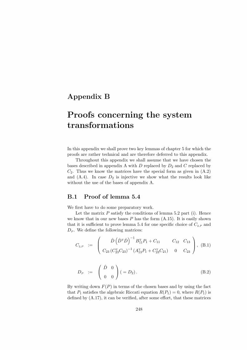
Appendix B
Proofs concerning the systemtransformations
In this appendix we shall prove two key lemmas of chapter 5 for which theproofs are rather technical and are therefore deferred to this appendix.
Throughout this appendix we shall assume that we have chosen thebases described in appendix A with D replaced by D2 and C replaced byC2. Thus we know the matrices have the special form as given in (A.2)and (A.4). In case D2 is injective we show what the results look likewithout the use of the bases of appendix A.
B.1 Proof of lemma 5.4
We first have to do some preparatory work.Let the matrix P satisfy the conditions of lemma 5.2 part (i). Hence
we know that in our new bases P has the form (A.15). It is easily shownthat it is sufficient to prove lemma 5.4 for one specific choice of C2,P andDP . We define the following matrices:
C2,P :=
D
(DTD
)−1BT
11P1 + C11 C12 C13
C23 (CT23C23)
−1 (AT13P1 + CT
23C21) 0 C23
, (B.1)
DP :=
D 0
0 0
( = D2) . (B.2)
By writing down F (P ) in terms of the chosen bases and by using the factthat P1 satisfies the algebraic Riccati equation R(P1) = 0, where R(P1) isdefined by (A.17), it can be verified, after some effort, that these matrices
248

B.1 Proof of lemma 5.4 249
indeed satisfy (5.3). In case D2 is injective we define the matrices C2,P
and DP without making use of the bases of appendix A by
C2,P := D2 (DT2D2)
−1 (BTP +DT2C2) , (B.3)
DP := D2. (B.4)
Next, we define the following matrices:
A := A11 −A13 (CT23C23)
−1 (AT13P1 + CT
23C21)
−B11
(DTD
)−1BT
11P1,
C1 := −(DT
)−1BT
11P1,
C2 := C21 − C23 (CT23C23)
−1 (AT13P1 + CT
23C21) ,
B11 := B11D−1,
B12 := A13 (CT23C23)
−1 CT23 − P
†1C
T21
(I − C23 (CT
23C23)−1CT
23
),
where † denotes the Moore–Penrose inverse. We now define the followingsystem:
ΣU :
xU = AxU +(B11 B12
)uU + E1wU ,
yU = −ET1P1xU + wU ,
zU =
(C1
C2
)xU +
(I 00 I
)uU .
(B.5)
In case D2 and D1 are injective and surjective respectively we can definethe above system ΣU without the bases of appendix A by
ΣU :
xU = AxU + B(DT2D2)−1DT
2 uU + EwU ,
yU = −ETPxU + wU ,
zU = C2xU + uU ,
(B.6)
where
A := A−B(DT2D2)−1(BTP +DT
2C2),C2 := C2 −D2(DT
2D2)−1(BTP +DT2C2).
We have the following properties of the system ΣU :

250 Proofs concerning the system transformations
Lemma B.1 : The system ΣU is inner. Let U denote the transfer matrixof ΣU . If we decompose U :
U
(wU
uU
)=:
(U11 U12
U21 U22
)(wU
uU
)=
(zU
yU
),
compatible with the sizes of uU , wU , yU , and zU then we have U−121 ∈ H∞
and U22 is strictly proper. ✷
Proof : By corollary A.8 we know that A is asymptotically stable andhence ΣU is internally stable. Moreover by theorem A.6 the matrixZ(P1) = A + E1E
T1 P1 is asymptotically stable and therefore we have
U−121 ∈ H∞. The fact that U22 is strictly proper is trivial. It is easy to
check, using lemma A.6 part (ii), that P1 is the observability gramian ofΣU . Moreover we have
(
00
) (I 00 I
)
I(0 0
)−ET
1 P1(C1
C2
)+
(BT
11
BT12
)
ET1
P1 = 0.
This can be checked by simply writing out and using the fact that
kerP1 ⊂ ker(I − C23 (CT
23C23)−1 CT
23
)C21.
The result that ΣU is inner then follows by applying lemma 2.10.
Proof of lemma 5.4 : We have our special choice of C2,P and DP
given by (B.1) and (B.2). As already noted, taking this special choicefor CP and DP is not essential. We shall first compare the following twosystems:
Σ
ΣPΣF
ΣF
ΣU
❄
✛
✻
✛
❄
✛
✻
✛
❄✻
y
z w
u
zU
yP uP
wU
yU = wP uU = zP
(B.7)

B.2 Proof of lemma 5.5 251
The system on the left is the same as the system on the left in (5.5) andthe system on the right is described by the system (B.5) interconnectedwith the system on the right in (5.5). We decompose the state of Σ, xinto x1, x2 and x3 according to the choice of bases described in appendixA and decompose the state of ΣP into x
1,P, x
2,P, x
3,Pwith respect to the
same basis (note that Σ and ΣP have the same state space Rn). Writingout all the differential equations using the decompositions of the matricesgiven in (A.2),(A.4) we find the following realization for the system onthe right in (B.7):
x
U− x1,P
xP
p
=
A + E1ET
1 P1 0 0
∗ A + BNC1 BM
∗ LC1 K
x
U− x1,P
xP
p
+
0
E + BND1
LD1
w
U
z =(
∗ C2 + D2NC1 D2M)x
U− x1,P
xP
p
+ D2ND1wU
The * denotes matrices which are unimportant for this argument. If wealso derive the system equations for the system on the left in (B.7) we seeimmediately that, since A+E1E
T1 P1 is asymptotically stable, the system
on the left is internally stable if, and only if, the system on the right isinternally stable. Moreover, if we take zero initial conditions and bothsystems have the same input w, then we have z = zU , i.e. the input–output behaviour of both systems is identical. Hence the system on theleft has H∞ norm less than 1 if, and only if, the system on the right hasH∞ norm less than 1.
By lemma B.1 we may apply lemma 2.12 to the system on the rightin (B.7) and hence we find that the closed-loop system is internally sta-ble and has H∞ norm less than 1 if, and only if, the dashed system isinternally stable and has H∞ norm less than 1.
Since the dashed system is exactly the system on the right in (5.5)and the system on the left in (B.7) is exactly equal to the system on theleft in (5.5) we have completed the proof.
B.2 Proof of lemma 5.5
We are now going to prove lemma 5.5. In fact, we shall prove the dualversion of this lemma since this is much more convenient for us. Otherwisewe would have to introduce a decomposition dual to the one used in

252 Proofs concerning the system transformations
appendix A and based on the weakly unobservable subspace. We firstfactorize G(Q):
G(Q) :=
(EQ
DQ
)(ET
QDT
Q
).
Define AQ := A+QCT2C2 and BQ := B +QCT
2D2 and the system:
ΣQ :
xQ = AQxQ + BQuQ + EQwQ,
yQ = C1xQ + DQwQ,
zQ = C2xQ + D2uQ.
(B.8)
First of all, we know that ΣF stabilizes Σ if, and only if, ΣTF stabilizes
ΣT. Moreover, we know that ‖G‖∞ = ‖GT‖∞. Hence we can derive thefollowing dualized version of lemma 5.4 for this dual system ΣQ:
Lemma B.2 : Let Q satisfy lemma 5.2 part (ii). Moreover let an ar-bitrary dynamic compensator ΣF be given, described by (2.4). Let thefollowing two systems be given where the system on the left is the inter-connection of (5.1) and (2.4) and the system on the right is the intercon-nection of (B.8) and (2.4).
Σ
ΣF
❄
✛
✻
✛
y
z w
u
ΣQ
ΣF
❄
✛
✻
✛
yQ
zQ wQ
uQ
Then the following statements are equivalent :
(i) The system on the left is internally stable and its transfer matrixhas H∞ norm less than 1.
(ii) The system on the right is internally stable and its transfer matrixhas H∞ norm less than 1. ✷
We shall now investigate what the matrices appearing in the matrix in-equality and the rank conditions look like for this new system ΣQ:
F (X) :=
AT
QX +XAQ + CT
2C2 +XEQETQX XBQ + CT
2D2
BTQX +DT
2C2 DT2D2
,
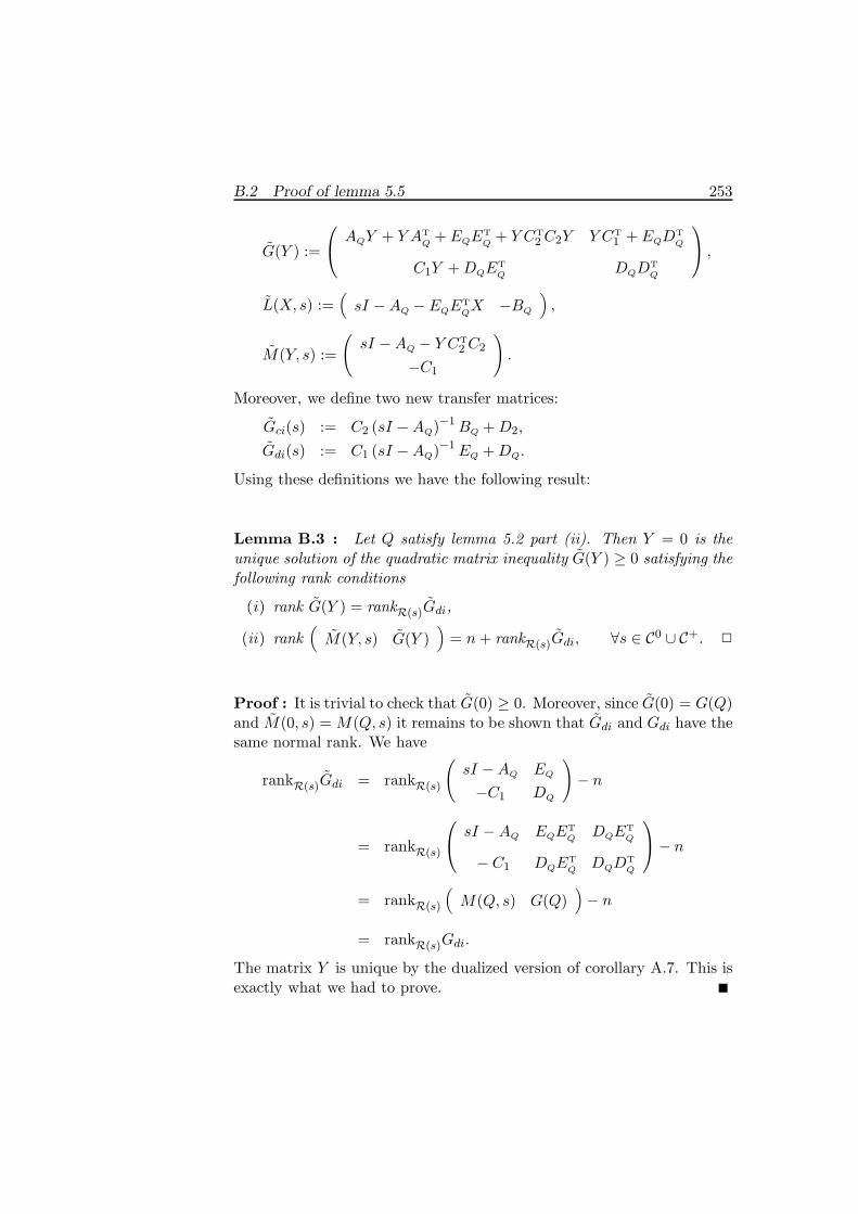
B.2 Proof of lemma 5.5 253
G(Y ) :=
AQY + Y AT
Q+ EQE
TQ+ Y CT
2C2Y Y CT1 + EQD
TQ
C1Y +DQETQ
DQDTQ
,
L(X, s) :=(sI −AQ − EQE
TQX −BQ
),
M(Y, s) :=
(sI −AQ − Y CT
2C2
−C1
).
Moreover, we define two new transfer matrices:
Gci(s) := C2 (sI −AQ)−1BQ +D2,
Gdi(s) := C1 (sI −AQ)−1EQ +DQ.
Using these definitions we have the following result:
Lemma B.3 : Let Q satisfy lemma 5.2 part (ii). Then Y = 0 is theunique solution of the quadratic matrix inequality G(Y ) ≥ 0 satisfying thefollowing rank conditions
(i) rank G(Y ) = rankR(s)Gdi,
(ii) rank(M(Y, s) G(Y )
)= n+ rankR(s)Gdi, ∀s ∈ C0 ∪ C+. ✷
Proof : It is trivial to check that G(0) ≥ 0. Moreover, since G(0) = G(Q)and M(0, s) =M(Q, s) it remains to be shown that Gdi and Gdi have thesame normal rank. We have
rankR(s)Gdi = rankR(s)
(sI −AQ EQ
−C1 DQ
)− n
= rankR(s)
sI −AQ EQE
TQ
DQETQ
− C1 DQETQ
DQDTQ
− n
= rankR(s)
(M(Q, s) G(Q)
)− n
= rankR(s)Gdi.
The matrix Y is unique by the dualized version of corollary A.7. This isexactly what we had to prove.

254 Proofs concerning the system transformations
Lemma B.4 : There is a solution X of the matrix inequality F (X) ≥ 0satisfying the following two rank conditions:
(i) rank F (X) = rankR(s)Gci,
(ii) rank
(L(X, s)F (X)
)= n+ rankR(s)Gci, ∀s ∈ C0 ∪ C+,
if, and only if, I−PQ is invertible. Moreover in that case the solution isunique and is given by X = (I − PQ)−1 P . We have X ≥ 0 if, and onlyif:
ρ (PQ) < 1. ✷
Proof : We first make a transformation on F (X):
Ftr(X) :=
(I (I +XQ)FT
0
0 I
)F (X)
(I 0
F0 (I +QX) I
)
=
(ATX +XA+ CT
2 C2 +XMX XB
BTX DT2D2
)
where,
A := A+BF0 +Q (C2 +D2F0)T (C2 +D2F0) ,
C2 := C2 +D2F0,
M := (A+BF0)Q+Q (AT + FT0 B
T) + EET +QCT2 C2Q,
and F0 as defined in (A.1). We also transform the second matrix appear-ing in the rank conditions:
W (X, s) :=
I 0 −QFT
0
0 I (I +XQ)FT0
0 0 I
(L(X, s)F (X)
)(I 0
F0 (I +QX) I
)
=
sI − A−MX −BATX +XA+ CT
2 C2 +XMX XB
BTX DT2D2
.

B.2 Proof of lemma 5.5 255
We have the following equality:
rankR(s)Gci = rankR(s)
(sI −AQ −BQ
C2 D2
)− n
= rankR(s)
(I QCT
2
0 I
)(sI −AQ −BQ
C2 D2
)− n
= rankR(s)
(sI −A −BC2 D2
)− n = rankR(s)Gci.
Therefore the conditions that X ≥ 0 has to satisfy can be reformulatedas:
(i) Ftr(X) ≥ 0
(ii) rank Ftr(X) = rankR(s)Gci
(iii) rank W (X, s) = rankR(s)Gci + n, ∀s ∈ C0 ∪ C+.
Moreover, we note that T (A,B,C2,D2) = T (A,B, C2,D2). This can beshown by using the fact that the new system is obtained by a state feed-back and an output injection (note that B = B + Q(C2 + D2F0)TD2)and the well-known fact that the strongly controllable subspace is invari-ant under state feedback and output injection. This can be easily shownusing the algorithm (2.15). We now choose the bases from appendix Awhere again C is replaced by C2 and D is replaced by D2. By lemma A.5we know that if X exists, then it will have the form:
X =
X1 0 00 0 00 0 0
, (B.9)
for some positive semi-definite matrix X1. Note that there is small differ-ence since M is not necessarily positive semi-definite but it is easy to seefrom the proof of lemma A.5 that this difference is not important. Weuse this decomposition for X and the corresponding decompositions forP and Q:
P =
P1 0 00 0 00 0 0
, Q =
Q11 Q12 Q13
Q21 Q22 Q23
Q31 Q32 Q33
.

256 Proofs concerning the system transformations
Together with the decompositions for the other matrices as given in (A.2)and (A.4) we can decompose Ftr(X) correspondingly:
X1A11 + AT11X1 + CT
21C21 +X1M11X1 0 X1A13 + CT21C23 X1B11 0
0 0 0 0 0AT
13X1 + CT23C21 0 CT
23C23 0 0BT
11X1 0 0 DTD 00 0 0 0 0
where
A11 := A11 +Q11CT21C21 +Q13C
T23C21,
A13 := A13 +Q11CT21C23 +Q13C
T23C23,
M11 := A11Q11 +A13QT13 +Q11A
T11 +Q13A
T13 + E1E
T1
+Q11CT21 (C21Q11 + C23Q13) +Q13C
T23 (C21Q11 + C23Q13) .
The rank condition: rank Ftr(X) = rankR(s)Gci is, according to lemmaA.4, equivalent with the condition that the rank of the above matrix isequal to the rank of the submatrix:
(CT
23C23 00 DTD
).
Therefore the Schur complement with respect to this submatrix shouldbe zero. This implies that if we define:
R(X1) := X1A11 + AT11X1 + CT
21C21
+X1
(M11 −B11
(DTD
)−1BT
11
)X1
−(X1A13 +CT
21C23
)(CT
23C23)−1
(AT
13X1 + CT23C21
)
then X1 should satisfy R(X1) = 0. Moreover, if we decompose W (X, s)correspondingly, then we can show by using elementary row and columnoperations that for any matrix X in the form (B.9), where X1 satisfiesR(X1) = 0, and for all s ∈ C, the matrix W (X, s) has the same rank as

B.2 Proof of lemma 5.5 257
the following matrix:
sI − Z(X1) 0 0 0 0∗ sI −A22 −A23 0 −B22
∗ −A32 sI −A33 0 −B32
0 0 0 0 00 0 0 0 00 0 I 0 00 0 0 I 00 0 0 0 0
, (B.10)
where
Z(X1) := A11 +M11X1 −B11
(DTD
)−1BT
11X1
−A13 (CT23C23)
−1(AT
13X1 + CT23C21
).
The matrix:sI −A22 −A23 −B22
−A32 sI −A33 −B32
0 I 0
,
has full row rank for all s ∈ C by lemma A.2 part (ii) and lemma 2.8.Hence the rank of the matrix (B.10) is n+rankR(s)Gci for all s ∈ C+∪C0
if, and only if, the matrix Z(X1) is asymptotically stable. Using this wecan now reformulate the conditions that X1 ≥ 0 has to satisfy:
(i) R(X1) = 0
(ii) Z(X1) is asymptotically stable.
In other words X1 should be the positive semi-definite stabilizing solutionof the algebraic Riccati equation R(X1) = 0. Denote the Hamiltoniancorresponding to this ARE by Hnew. We know that P1 is the stabilizingsolution of the algebraic Riccati equation R(P1) = 0 as given by (A.17).Denote the Hamiltonian corresponding to this algebraic Riccati equationby Hold. Then it can be checked that:
Hold =
(I Q11
0 I
)Hnew
(I −Q11
0 I
). (B.11)

258 Proofs concerning the system transformations
Since P1 is the stabilizing solution of the Riccati equation correspond-ing to the Hamiltonian Hold we know that the modal subspace of Hold
corresponding to the open left half plane is given by:
Xg(Hold) = Im
(I
P1
). (B.12)
Combining (B.11) and (B.12) we find:
Xg(Hnew) = Im
(I −Q11
0 I
)(I
P1
)= Im
(I −Q11P1
P1
).
Therefore we know that a stabilizing solution to the algebraic Riccatiequation R(X1) = 0 exists if, and only if, I−Q11P1 is invertible and in thiscase the solution is given by X1 = P1 (I −Q11P1)
−1. This implies thatX = P (I −QP )−1 = (I − PQ)−1 P . The requirement X ≥ 0 is satisfiedif, and only if, ρ(PQ) < 1, which can be checked straightforwardly. Thiscompletes the proof.

Bibliography
[AM] B.D.O. Anderson, J.B. Moore, Optimal control: linear quadraticmethods, Prentice-Hall, 1989.
[Ban] M.D. Banker, Observability and controllability of two player dis-crete systems and quadratic control and game problems, Ph.D.Thesis, Stanford Univ, Stanford, CA, 1971.
[Bas] T. Basar, “A dynamic games approach to controller design: dis-turbance rejection in discrete time”, Proc. CDC, Tampa, FL,1989, pp. 407–414.
[BB] T. Basar, P. Bernhard, H∞ -optimal control and related minimaxdesign problems: a dynamic game approach, Birkhauser, Boston,1991.
[BBK] S. Boyd, V. Balakrishnan, P. Kabamba, “A bisection methodfor computing the H∞ -norm of a transfer matrix and relatedproblems”, Math. Contr. Sign. & Syst., Vol. 2, 1989, pp. 207–219.
[BC] J.A. Ball, N. Cohen, “Sensitivity minimization in the H∞ norm:parametrization of all suboptimal solutions”, Int. J. Contr., Vol.46, 1987, pp. 785–816.
[Bel] R. Bellman, Introduction to matrix analysis, 2nd ed., McGraw-Hill, New York, 1970.
[BH] D.S. Bernstein, W.M. Haddad, “Steady state Kalman filteringwith an H∞ error bound”, Syst. & Contr. Letters, Vol. 12, 1989,pp. 9–16.
[BH2] D.S. Bernstein, W.M. Haddad, “LQG control with anH∞ perfor-mance bound: A Riccati equation approach”, IEEE Trans. Aut.Contr., Vol. 34, No. 3, 1989, pp. 293–305.
259

260 Bibliography
[Bo] P. Boekhoudt, The H∞ control design method: a polynomial ap-proach, Ph.D. Thesis, University of Twente, Enschede, 1988.
[BO] T. Basar, G.J. Olsder, Dynamic noncooperative game theory, Aca-demic Press, New York, 1982.
[BS] N.A. Bruinsma, M. Steinbuch, “A fast algorithm to compute theH∞ norm of a transfer matrix”, Syst. & Contr. Letters, Vol. 14,1990, pp. 287–293.
[BvS] A. Bensoussan, J.H. van Schuppen, “Optimal control of partiallyobservable stochastic systems with an exponential–of–integralperformance index”, SIAM J. Contr. & Opt., Vol. 23, No. 4, 1985,pp. 599–613.
[BW] D. Biss, K.G. Woodgate, “Gas turbine control using mixed-sensitivity H∞ optimization”, Robust control of linear systemsand nonlinear control, Proc. MTNS-89, Vol II, M.A. Kaashoek,J.H. van Schuppen, A.C.M. Ran (eds.), Birkhauser, Boston, 1990,pp. 255– 265.
[Ch] T. Chen, B.A. Francis, “On the L2-induced norm of a sampled-data system”, Syst. & Contr. Letters, Vol. 15, 1990, pp. 211–220.
[Ch2] T. Chen, B.A. Francis, “H2-optimal sampled-data control”, IEEETrans. Aut. Contr., Vol. 36, No. 4, 1991, pp. 387–397.
[Cr] J.W. van Crevel, “Control design for a 90 MW coal fired fluidizedbed boiler”, Cambridge Control Ltd., Report no. 36-R82/2, 1989.
[CS] R.Y. Chiang, M.G. Safonov, Robust control toolbox user’s guide,The Mathworks Inc., Sherborn, MA, 1988.
[Do] J.C. Doyle, G. Stein, “Multivariable feedback design: conceptsfor a classical/modern synthesis”, IEEE Trans. Aut. Contr., Vol.26, No. 1, 1981, pp. 4–16.
[Do2] J.C. Doyle, “Analysis of feedback systems with structured uncer-tainties”, IEE Proc., Vol. 129, Part D, 1982, pp. 242–250.
[Do3] J.C. Doyle, “Lecture notes in advances in multivariable control”,ONR/Honeywell Workshop, Minneapolis, 1984.
[Do4] J.C. Doyle, K. Zhou, B. Bodenheimer, “Optimal control withmixed H2 and H∞ performance objectives”, Proc. ACC, Pitts-burgh, PA, 1989, pp. 2065–2070.

Bibliography 261
[Do5] J. Doyle, K. Glover, P.P. Khargonekar, B.A. Francis, “State spacesolutions to standardH2 andH∞ control problems”, IEEE Trans.Aut. Contr., Vol. 34, No. 8, 1989, pp. 831–847.
[Fa] P.L. Faurre “Stochastic realization algorithms”, System Identifi-cation: advances and case studies, R.K. Mehra, D.G. Lainiotis(eds.), Academic Press, New York, 1976, pp. 1–25.
[FL] J.S. Freudenberg, D.P. Looze, “Right half plane poles and ze-ros and design tradeoffs in feedback systems”, IEEE Trans. Aut.Contr., Vol. 30, No. 6, 1985, pp. 555–565.
[Fr] B.A. Francis, “The optimal linear-quadratic time invariant reg-ulator with cheap control”, IEEE Trans. Aut. Contr., Vol. 24,1979, pp. 616–621.
[Fr2] B.A. Francis, A course in H∞ control theory, Lecture notes incontrol and information sciences, Vol 88, Springer Verlag, Berlin,1987.
[Ga] F.R. Gantmacher, The theory of matrices, Chelsea, New York,1959.
[Gee] T. Geerts, “All optimal controls for the singular linear-quadraticproblem without stability; a new interpretation of the optimalcost”, Lin. Alg. Appl., Vol. 122, 1989, pp. 65–104.
[Gen] Y. Genin, P. van Dooren, T. Kailath, J.M. Delosme, M. Morf,“On Σ-lossless transfer functions and related questions”, Lin. Alg.Appl., Vol. 50, 1983, pp. 251–275.
[GK] G. Gu, P.P. Khargonekar, “A class of algorithms for identificationin H∞ ”, To appear in Automatica.
[GK2] G. Gu, P.P. Khargonekar, “Linear and nonlinear algorithms foridentification in H∞ with error bounds”, To appear in IEEETrans. Aut. Contr..
[Gl] K. Glover, “All optimal Hankel-norm approximations of linearmultivariable systems and their L∞-error bounds”, Int. J. Contr.,Vol. 39, 1984, pp. 1115–1193.
[Gl2] K. Glover, “Robust stabilization of multivariable linear systems:relations to approximation”, Int. J. Contr., Vol. 43, 1986, pp.741–766.

262 Bibliography
[Gl3] K. Glover, J. Doyle, “State-space formulaes for all stabilizing con-trollers that satisfy an H∞ norm bound and relations to risksensitivity”, Syst. & Contr. Letters, Vol. 11, 1988, pp. 167–172.
[Gl4] K. Glover, D. Mc.Farlane, “Robust stabilization of normalizedcoprime factor plant description with H∞ -bounded uncertainty”,IEEE Trans. Aut. Contr., Vol. 34, 1989, pp. 821–830.
[Gl5] K. Glover, “Minimum entropy and risk-sensitive control: the con-tinuous time case”, Proc. CDC, Tampa, FL, 1989, pp. 388–391.
[Gl6] K. Glover, D.J.N. Limebeer, J.C. Doyle, E.M. Kasenally, M.G.Safonov, “A characterization of all solutions to the four blockgeneral distance problem”, SIAM J. Contr. & Opt., Vol. 29, No.2, 1991, pp. 283–324.
[Gr] M. Green, D.J.N. Limebeer, “Vector interpolation, H∞ controland model reduction”, Robust control of linear systems and non-linear control, Proc. MTNS-89, Vol II, M.A. Kaashoek, J.H. vanSchuppen, A.C.M. Ran (eds.), Birkhauser, Boston, 1990, pp. 285–292.
[Gr2] M. Green, K. Glover, D.J.N. Limebeer, J.C. Doyle, “A J-spectralfactorization approach to H∞ control”, SIAM J. Contr. & Opt.Vol. 28, No. 6, 1990, pp. 1350–1371.
[Gri] M.J. Grimble, “Optimal robustness and the relationship to LQGdesign problems”, Int. J. Contr., Vol. 43, 1986, pp. 351–372.
[GS] T.T. Georgiou, M.C. Smith, “Optimal robustness in the gap met-ric”, Proc. CDC, Tampa, FL, 1989, pp. 2331–2336.
[Gu] D.W. Gu, M.C. Tsai, S.D. O’Young, I. Postelthwaite, “Statespace formulae for discrete time H∞ optimization”, Int. J.Contr., Vol. 49, 1989, pp. 1683–1723.
[Ha] M.L.J. Hautus, “Strong detectability and observers”, Lin. Alg. &Appl., Vol. 50, 1983, pp. 353–368.
[Hab] L.C.G.J.M. Habets, Robust stabilization in the gap topology, Lec-ture notes in control and information sciences, Vol. 150, SpringerVerlag, Berlin, 1991.
[HB] W.M. Haddad, D.S. Bernstein, “Combined L2/H∞ model reduc-tion”, Int. J. Contr., Vol. 49, 1989, pp. 1523–1535.

Bibliography 263
[HB2] W.M. Haddad, D.S. Bernstein, “Generalized Riccati equations forthe full- and reduced-order mixed-norm H2/H∞ standard pro-blem”, Syst. & Contr. Letters, Vol. 14, 1990, pp. 185–197.
[Hi] D. Hinrichsen, A.J. Pritchard, “Real and complex stability radii:a survey”, Control of Uncertain Systems, Proc. InternationalWorkshop, Bremen, 1989, Birkhauser, Boston, 1990, pp. 119–162.
[HJN] A.J. Helmicki, C.A. Jacobson, C.N. Nett, “Control oriented sys-tem identification: a worst case/deterministic approach in H∞ ”,IEEE Trans. Aut. Contr., Vol. 36, 1991, pp. 1163–1176.
[Ho] K. Hoffman, Banach spaces of analytic functions, Prentice-Hall,Englewoods Cliffs, NJ, 1962.
[Hor] I.M. Horowitz, Synthesis of feedback systems, Academic Press,New York, 1963.
[HSK] S. Hara, T. Sugie, R. Kondo, “Descriptor form solution for H∞control problem with jω-axis zeros”, To appear in Automatica.
[Ig] P.A. Iglesias, K. Glover, “State space approach to discrete timeH∞ control”, To appear in Int. J. Contr., 1991.
[KA] J.P. Keller, B.D.O. Anderson, “A new approach to discretizationof continuous-time controllers”, Proc. ACC, San Diego, CA, 1990,pp. 1133–1136.
[Kh] P.P. Khargonekar, A. Tannenbaum, “Non-Euclidian metrics andthe robust stabilization of systems with parameter uncertainty”,IEEE Trans. Aut. Contr., Vol. 30, 1985, pp. 1005–1013.
[Kh2] P.P. Khargonekar, I.R. Petersen, K. Zhou, “Robust stabilizationof uncertain systems and H∞ optimal control”, Proc. AllertonConf. on Comm., Contr. & Comp., Monticello, IL, 1987, pp. 88–95.
[Kh3] P.P. Khargonekar, I.R. Petersen, M.A. Rotea, “H∞ optimal con-trol with state feedback”, IEEE Trans. Aut. Contr., Vol. 33, 1988,pp. 786–788.
[Kh4] P.P. Khargonekar, “State-space H∞ control theory”, Mathemati-cal system theory: the influence of R.E. Kalman, Edited by A.C.Antoulas, Springer Verlag, Berlin, 1991.

264 Bibliography
[Kh5] P.P. Khargonekar, I.R. Petersen, K. Zhou, “Robust stabilizationof uncertain linear systems: quadratic stabilizability andH∞ con-trol theory”, IEEE Trans. Aut. Contr., Vol. 35, 1990, pp. 356–361.
[Kh6] P.P. Khargonekar, M.A. Rotea, “Mixed H2 /H∞ control: a con-vex optimization approach”, IEEE Trans. Aut. Contr., Vol. 36,1991, pp. 824–837.
[KH] P. Kabamba, S. Hara, “On computing the induced norm of asampled data system”, Proc. ACC, San Diego, CA, 1990, pp.319–320.
[Ki] H. Kimura, “Conjugation, interpolation and model-matching inH∞ ”, Int. J. Contr., Vol. 49, 1989, pp. 269–307.
[Ku] V. Kucera, “A contribution to matrix quadratic equations”, IEEETrans. Aut. Contr., Vol. 17, 1972, pp. 344–347.
[Kw] H. Kwakernaak, “A polynomial approach to minimax frequencydomain optimization of multivariable feedback systems”, Int. J.Contr., Vol. 41, 1986, pp. 117–156.
[Kw2] H. Kwakernaak, “Progress in the polynomial solution of thestandard H∞ optimal control problem”, Proceedings 11th IFACWorld Congress, Vol. 5, Ed. V. Utkin, U. Jaaksoo, Tallinn, USSR,1990, pp. 122–129.
[Li] D.J.N. Limebeer, Y.S. Hung, “An analysis of the pole-zero cancel-lations in H∞ optimal control problems of the first kind”, SIAMJ. Contr. & Opt., Vol. 25, 1987, pp. 1457–1493.
[Li2] D.J.N. Limebeer, G.D. Halikias, “A controller degree bound forH∞ control problems of the second kind”, SIAM J. Contr. &Opt., Vol. 26, 1988, pp. 646–677.
[Li3] D.J.N. Limebeer, B.D.O. Anderson, “An interpolation theory ap-proach to H∞ controller degree bounds”, Lin. Alg. Appl., Vol.98, 1988, pp. 347–386.
[Li4] D.J.N. Limebeer, M. Green, D. Walker, “Discrete time H∞ con-trol”, Proc. CDC, Tampa, FL, 1989, pp. 392–396.
[Li5] D.J.N. Limebeer, B.D.O. Anderson, P.P. Khargonekar, M. Green,“A game theoretic approach to H∞ control for time-varying sys-tems”, To appear in SIAM J. Contr. & Opt.

Bibliography 265
[LM] E.B. Lee, L. Markus, Foundations of optimal control theory, Wi-ley, New York, 1967.
[LMK] K.Z. Liu, T. Mita, H. Kimura, “Complete solution to the standardH∞ control problem of discrete time systems”, 1990, submittedfor publication.
[M] J. Maciejowski, Multivariable feedback design, Addison-Wesley,Reading, MA, 1989.
[Ma] E.F. Mageirou, “Values and strategies for infinite time linearquadratic games”, IEEE Trans. Aut. Contr., Vol. 21, 1976, pp.547–550.
[MF] D.C. McFarlane, K. Glover, Robust controller design using nor-malized coprime factor descriptions, Lecture notes in control andinformation sciences, Vol 138, Springer Verlag, Berlin, 1990.
[Mo] B.P. Molinari, “Nonnegativity of a quadratic functional”, SIAMJ. Contr. & Opt., Vol. 13, 1975, pp. 792–806.
[Mu] D. Mustafa, K. Glover Minimum entropy H∞ control, Lecturenotes in control and information sciences, Vol 146, Springer Ver-lag, Berlin, 1990.
[Mu2] D. Mustafa, K. Glover, “Model reduction by H∞ -balanced trun-cation”, IEEE Trans. Aut. Contr., Vol. 36, No. 6, 1991, pp. 668–682.
[Ni] H.H. Niemann, P. Søgaard-Andersen, J. Stoustrup, “Loop trans-fer recovery: Analysis and design for general observer architec-tures”, To appear in Int. J. Contr.
[OM] R.E. O’Malley, Jr., Singular perturbation methods for ordinarydifferential equations, Springer-Verlag, Berlin, 1991.
[OSS1] H.K. Ozcetin, A. Saberi, P. Sannuti, “Design for almost distur-bance decoupling problem with internal stability via state or mea-surement feedback– singular perturbation approach”, To appearin Int. J. Contr.
[OSS2] H.K. Ozcetin, A. Saberi and Y. Shamash “An H∞ almost distur-bance decoupling technique for nonstrictly proper systems”, Toappear in Proc. CDC, Brighton, U.K., 1991.

266 Bibliography
[Pe] I.R. Petersen, C.V. Hollot, “A Riccati equation approach to thestabilization of uncertain linear systems”, Automatica Vol. 22,1986, pp. 397–411.
[Pe2] I.R. Petersen, “Linear quadratic differential games with cheapcontrol”, Syst. & Contr. Letters, Vol. 8, 1986, pp. 181–188.
[Pe3] I.R. Petersen, “Disturbance attenuation and H∞ optimization:a design method based on the algebraic Riccati equation”, IEEETrans. Aut. Contr., Vol. 32, No. 5, 1987, pp. 427–429.
[Pe4] I.R. Petersen, “Some new results on algebraic Riccati equationsarising in linear quadratic differential games and the stabilizationof uncertain systems”, Syst. & Contr. Letters, Vol. 10, 1988, pp.341–348.
[Pe5] I.R. Petersen, C.V. Hollot, “High gain observers applied to prob-lems in the stabilization of uncertain linear systems, disturbanceattenuation and H∞ optimization”, Int. J. Adapt. Contr. andSign. Proc., Vol. 3, 1989.
[PM] M.A. Peters, A time-domain approach to H∞ worst-case design,Masters Thesis, Eindhoven University of Technology, 1989.
[Re] R.M. Redheffer, “On a certain linear fractional transformation”,J. Math. and Physics, Vol. 39, 1960, pp. 269–286.
[RK] M.A. Rotea, P.P. Khargonekar, “H2 optimal control with an H∞constraint: the state feedback case”, Automatica, Vol. 27, No. 2,1991, pp. 307–316.
[RK2] M.A. Rotea, P.P. Khargonekar, “Stabilization of uncertain sys-tems with norm-bounded uncertainty: a control Lyapunov ap-proach”, SIAM J. Contr. & Opt., Vol. 27, 1989, pp. 1462–1476.
[RNK] R. Ravi, K. Nagpal, P.P. Khargonekar, “H∞ for linear time-varying systems: a state space approach”, To appear in SIAMJ. Contr. & Opt., Vol. 29, No. 6, 1991.
[Ro] H.H. Rosenbrock, “The zeros of a system”, Int. J. Contr., Vol.18, 1973, pp. 297–299 and correction Vol. 20, 1974, pp. 525–527.
[RR] M. Rosenblum, J. Rovnyak, Hardy classes and operator theory,Oxford University Press, New York, 1985.

Bibliography 267
[Ru] W. Rudin, Real and complex analysis, 3rd. ed., McGraw-Hill, NewYork, 1987.
[Sa] M.G. Safonov, “Imaginary axis zeros in multivariableH∞ optimalcontrol”, Proc. NATO Workshop on Modelling, Robustness andSensitivity Reduction in Control Systems, Groningen, 1986.
[SC] M.G. Safonov, R.Y. Chiang, “CACSD Using the state space L∞theory: a design example” IEEE Trans. Aut. Contr., Vol. 33, No.5, 1988, pp. 477–479.
[SC2] M.G. Safonov, R.Y. Chiang, H. Flashner, “H∞ robust controlsynthesis for a large space structure”, Proc. ACC, Atlanta, GA,1988, pp. 2038–2043.
[SLH] M.G. Safonov, A.J. Laub, G.L. Hartmann, “Feedback propertiesof multivariable systems: the role and use of the return differencematrix”, IEEE Trans. Aut. Contr., Vol. 26, No. 1, 1981, pp. 47–65.
[S] C. Scherer, “H∞ control by state feedback: An iterative al-gorithm and characterization of high gain occurence”, Syst. &Contr. Letters, Vol. 12, 1989, pp. 383–391.
[S2] C. Scherer, “H∞ control by state feedback and fast algorithmsfor the computation of optimal H∞ norms”, IEEE Trans. Aut.Contr., Vol. 35, 1990, pp. 1090–1099.
[S3] C. Scherer, “H∞ control by state feedback for plants with zeroson the imaginary axis”, To appear in SIAM J. Contr. & Opt.,Vol. 30, No. 1, 1991.
[S4] C. Scherer, “H∞ -optimization without assumptions on finite orinfinite zeros”, To appear in SIAM J. Contr. & Opt., Vol. 30, No.1, 1991.
[SE] E. Schijfs, A numerical analysis of the singular H∞ control pro-blem, Masters Thesis, Eindhoven University of Technology, 1990.
[SH] J.M. Schumacher, Dynamic feedback in finite and infinite dimen-sional linear systems, Math. Centre Tracts 143, Amsterdam, 1981.
[SH2] J.M. Schumacher, “The role of the dissipation matrix in singularoptimal control”, Syst. & Contr. Letters, Vol. 2, 1983, pp. 262–266.

268 Bibliography
[SH3] J.M. Schumacher, “On the structure of strongly controllable sys-tems”, Int. J. Contr., Vol. 38, 1983, pp. 525–545.
[SH4] J.M. Schumacher, “A geometric approach to the singular filteringproblem”, IEEE Trans. Aut. Contr., Vol. 30, 1985, pp. 1075–1082.
[Si] L.M. Silverman, “Discrete Riccati equations: alternative algo-rithms, asymptotic properties and system theory interpretation”,In Control and dynamic systems, Academic Press, New York, Vol.12, 1976, pp. 313–386.
[SK] N. Shivashankar, P.P. Khargonekar “Robust stabilization and per-formance analysis of sampled data systems”, To appear in Proc.CDC, Brighton, U.K., 1991, Submitted to IEEE Trans. Aut.Contr.
[SS] P. Sannuti and A. Saberi, A special coordinate basis of multivari-able linear systems — finite and infinite zero structure, squar-ing down and decoupling, Int. J. Contr., Vol.45, No.5, 1987, pp.1655–1704.
[St] A.A. Stoorvogel, “H∞ control with state feedback”, Robust con-trol of linear systems and nonlinear control, Proc. MTNS-89,Vol II, M.A. Kaashoek, J.H. van Schuppen, A.C.M. Ran (eds.),Birkhauser, Boston, 1990, pp. 347–354.
[St2] A.A. Stoorvogel, H.L. Trentelman, “The quadratic matrix in-equality in singular H∞ control with state feedback”, SIAM J.Contr. & Opt., Vol. 28, No. 5, 1990, pp. 1190–1208.
[St3] A.A. Stoorvogel, “The singular zero-sum differential game withstability using H∞ control theory”, Math. Contr. Sign. & Syst.,Vol. 4, No. 2, 1991, pp. 121–138.
[St4] A.A. Stoorvogel, “The singularH∞ control problem with dynamicmeasurement feedback”, SIAM J. Contr. & Opt.. Vol. 29, No. 1,1991, pp. 160–184.
[St5] A.A. Stoorvogel, “The discrete time H∞ control problem: thefull information case”, COSOR memorandum 89-25, EindhovenUniversity of Technology, October 1989.
[St6] A.A. Stoorvogel, “The discrete time H∞ control problem withmeasurement feedback”, To appear in SIAM J. Contr. & Opt.,Vol. 30, No. 1, 1991.

Bibliography 269
[St7] A.A. Stoorvogel, H.L. Trentelman, “The finite horizon singulartime-varying H∞ control problem with dynamic measurementfeedback”, COSOR memorandum 89-33, Eindhoven University ofTechnology, 1989.
[St8] A.A. Stoorvogel, “Robust stabilization of systems with multiplica-tive perturbations”, COSOR Memorandum 90-36, EindhovenUniversity of Technology, To appear in Proc. MTNS-91, Kobe,Japan, 1991.
[St9] A. A. Stoorvogel, The H∞ control problem: a state space ap-proach, Ph.D. Thesis, Department of Mathematics and Comput-ing Science, Eindhoven University of Technology, The Nether-lands, 1990.
[St10] A.A. Stoorvogel, “The singular minimum entropyH∞ control pro-blem”, Syst. & Contr. Letters, Vol. 16, No. 6, 1991, pp. 411–422.
[St11] A.A. Stoorvogel, J.W. van der Woude, “The disturbance decou-pling problem with measurement feedback and stability for sys-tems with direct feedthrough matrices”, Syst. & Contr. Letters,Vol. 17, No. 3, 1991, pp. 217–226.
[St12] A.A. Stoorvogel, “The singular H2 control problem”, To appearin Automatica, 1992.
[St13] A.A. Stoorvogel, A. Saberi, B.M. Chen, “A reduced order basedcontroller design for H∞ optimization”, Proc. AIAA Guidance,Navigation and Control Conference, New Orleans, LA, Vol. 2,1991, pp. 716-722.
[St14] A.A. Stoorvogel, H.L. Trentelman, “The mixed H2 and H∞ con-trol problem”, To appear in Proc. Workshop on Robust Control,Tokyo, Japan, 1991.
[St15] A.A. Stoorvogel, A.J.T.M. Weeren, “The discrete time Riccatiequation related to theH∞ control problem”, Submitted for pub-lication, September 1991.
[Sw] A.C.M. van Swieten, Qualitative behavior of dynamical gameswith feedback strategies, Ph.D. Thesis, University of Groningen,The Netherlands, 1977.
[Ta] G. Tadmor, “Worst-case design in the time domain: the max-imum principle and the standard H∞ problem”, Math. Contr.Sign. & Syst., Vol. 3, 1990, pp. 301–324.

270 Bibliography
[Tr] H.L. Trentelman, Almost invariant subspaces and high gain feed-back, CWI Tracts, Vol. 29, Amsterdam, 1986.
[Tr2] H.L. Trentelman, A.A. Stoorvogel, “Completion of the squaresin the finite horizon H∞ control problem by measurement feed-back”, New trends in system theory, Proc. of the Universita diGenova-The Ohio State University Joint Conference, G. Conte,A.M. Perdon, B. Wyman (eds.), Birkhauser, Boston, 1991, pp.692-699.
[Va] A. Varga, V. Ionescu, “HTOOLS- a toolbox for solving H∞ andH2 synthesis problems”, IFAC CADCS ’91 Symposium, Swansea,UK, 1991.
[Vi] M. Vidyasagar, Control System Synthesis: A factorization ap-proach, MIT Press, Cambridge, MA, 1985
[Wa] D.J. Walker, “Relationship between three discrete-time H∞ al-gebraic Riccati equation solutions”, Int. J. Contr., Vol. 52, 1990,pp. 801–809.
[WA] A.J.T.M. Weeren, Solving discrete time algebraic Riccati equa-tions, Masters Thesis, Eindhoven University of Technology, 1991.
[We] S. Weiland, “Linear quadratic games, H∞ and the Riccati equa-tion”, Proceedings of The Riccati equation in control, systems andsignals, Como, Italy, 1989, pp. 156–159.
[Wh] P. Whittle, “Risk-sensitive linear/quadratic/Gaussian control”,Adv. Appl. Prob., Vol. 13, 1981, pp. 764–777.
[Wi] J.C. Willems, “Least squares stationary optimal control and thealgebraic Riccati equation”, IEEE Trans. Aut. Contr., Vol. 16,1971, pp. 621–634.
[Wi2] J.C. Willems, The analysis of feedback systems, MIT Press, Cam-bridge, MA, 1971.
[Wi3] J.C. Willems, “Dissipative dynamical systems, part I: general the-ory”, Arch. Rational Mech. Anal., Vol. 45, 1972, pp. 321–351.
[Wi4] J.C. Willems, “Dissipative dynamical systems, part I: linear sys-tems with quadratic supply rates”, Arch. Rational Mech. Anal.,Vol. 45, 1972, pp. 352–393.

Bibliography 271
[Wi5] J.C. Willems, “Almost invariant subspaces: an approach to highgain feedback design– Part I: almost controlled invariant sub-spaces”, IEEE Trans. Aut. Contr., Vol. 26, 1981, pp. 235–252.
[Wi6] J.C. Willems, “Almost invariant subspaces: an approach to highgain feedback design– Part II: almost conditionally invariant sub-spaces”, IEEE Trans. Aut. Contr., Vol. 27, 1982, pp. 1071–1084.
[Wi7] J.C. Willems, A. Kitapci, L.M. Silverman, “Singular optimal con-trol: a geometric approach”, SIAM J. Contr. & Opt., Vol. 24,1986, pp. 323–337.
[Wo] W.M. Wonham, Linear multivariable control: a geometric ap-proach, 2nd ed., Springer Verlag, Berlin, 1979.
[WW] S. Weiland, J.C. Willems, “Almost disturbance decoupling withinternal stability”, IEEE Trans. Aut. Contr., Vol. 34, 1989, pp.277–286.
[WW2] S. Weiland, J.C. Willems, “Dissipative systems in a behaviouralcontext”, Math. Models and Methods in Applied Sciences, Vol. 1,No. 1, 1991, pp. 1–25.
[Ya] I. Yaesh, U. Shaked, “Minimum H∞ -norm regulation of lineardiscrete-time systems and its relation to linear quadratic discretegames”, IEEE Trans. Aut. Contr., Vol. 35, 1990, pp. 1061–1064.
[Yo] N. Young, An introduction to Hilbert space, Cambridge UniversityPress, Cambridge, 1988.
[Za] G. Zames, “Feedback and optimal sensitivity: model referencetransformations, multiplicative seminorms, and approximate in-verses”, IEEE Trans. Aut. Contr., Vol 26, 1981, pp. 301–320.
[Za2] G. Zames, B.A. Francis, “Feedback, minimax sensitivity and op-timal robustness”, IEEE Trans. Aut. Contr., Vol. 28, 1983, pp.585–600.
[Zh] S.Q. Zhu, Robustness of feedback stabilization: A topological ap-proach, Ph.D. Thesis, Department of Mathematics and Comput-ing Science, Eindhoven University of Technology, The Nether-lands, 1989.
[ZK] K. Zhou, P.P. Khargonekar, “Robust stabilization of linear sys-tems with norm bounded time varying uncertainty”, Syst. &Contr. Letters, Vol. 10, 1988, pp. 17–20.

272 Bibliography
[ZK2] K. Zhou, P.P. Khargonekar, “An algebraic Riccati equation ap-proach to H∞ optimization”, Syst. & Contr. Letters, Vol. 11,1988, pp. 85–91.
[ZK3] K. Zhou, J. Doyle, K. Glover, B. Bodenheimer, “Mixed H2 andH∞ control”, Proc. ACC, San Diego, CA, 1990, pp. 2502–2507.

Index
∼ . . . . . . . . . . . . . . . . . . . . . . . . . . 23‖ · ‖ . . . . . . . . . . . . . . . . . . . . . . . . 31‖ · ‖1 . . . . . . . . . . . . . . . . . . . . . . . 42‖ · ‖2 . . . . . . . . . . . . . . . . . . . . 31,37‖ · ‖∞ . . . . . . . . . . . . . . . . . . 7,30,36AF0 . . . . . . . . . . . . . . . . . . . . . . . 235A-invariant . . . . . . . . . . . . . . . . . 25(A,B)-invariant . . . . . . . . . . . . 25ADDPMS . . . . . . . . . . . . . . . . . . 40ADDPS . . . . . . . . . . . . . . . . . . . . 39additive perturbations . . . . . 206adjoint operator . . . . . . . . . . . 159admissible pair . . . . . . . . . . . . 122asymptotically stable . . . . 20,21backwards difference
equation . . . . . . . . . . . . . . . 22Bode diagram . . . . . . . . . . . . . . . 9C . . . . . . . . . . . . . . . . . . . . . . . . . . . 17C+ ( C0, C− ) . . . . . . . . . . . . . . . 17C∞
0 . . . . . . . . . . . . . . . . . . . . . . . . . 24C−1X . . . . . . . . . . . . . . . . . . . . . . 27CF0 . . . . . . . . . . . . . . . . . . . . . . . 235(C,A)-invariant . . . . . . . . . . . . 25causal . . . . . . . . . . . . . . . . . . . . . 168
strictly . . . . . . . . . . . . . . . . 168non- . . . . . . . . . . . . . . . . . . 230
central controller . . . 12,107,140co-inner . . . . . . . . . . . . . . . . . . . . 32complex stability radius . . . 213conditioned invariant . . . . . . . 25controllability pencil . . . . . . . . 24controlled invariant . . . . . . . . . 25control sensitivity function . . . 9coprime-factor perturbations . 7
normalized . . . . . . . . . . . . . . 7D (δD, D+) . . . . . . . . . . . . . . . . 17DDPMS . . . . . . . . . . . . . . . . . . . . 40DDPS . . . . . . . . . . . . . . . . . . . . . . 39detectable strongly
controllable subspace . . . 26deterministic error . . . . . . . . . . . 2differential game . . . . . . . . . . . . 13direct-feedthrough matrix 20,22discrete time systems . . . . . . . 15dissipation inequality . . . . . . . 68distance of systems . . . . . . . . . . 6disturbance decoupling . 39,200
almost . . . . . . . . . . . . . . 12,39dual . . . . . . . . . . . . . . . . . . . . . . . . 21dual subspaces . . . . . . . . . . . . . 25dualization . . . . . . . . . . . . . . . . 159E . . . . . . . . . . . . . . . . . . . . . . . . . 143entropy function . . . . . . . 139,140entropy at infinity . . . . . . . . . 142equilibrium . . . . . . . . . . . . . . . . 122
almost . . . . . . . . . . . . . . . . 123finite horizon H∞
control problem . . . . 15,154frequency spectrum . . . . . . . . . . 9gap metric . . . . . . . . . . . . . . . . . . . 7gap topology . . . . . . . . . . . . . . . . 7Gaussian process . . . . . . . . . . . . 2graph topology . . . . . . . . . . . . . . 7H2 . . . . . . . . . . . . . . . . . . . . . . . . . 30H2 norm . . . . . . . . . . . . . . . . . 14,30H1
2 . . . . . . . . . . . . . . . . . . . . . . . . . 30H∞ . . . . . . . . . . . . . . . . . . . . . 30,36H∞ norm . . . . . . . . . . . . 3,9,30,36
273

274 Index
H1∞ . . . . . . . . . . . . . . . . . . . . . 29,36Hardy spaces . . . . . . . . . . . . . . . 30inner . . . . . . . . . . . . . . . . . . . . 32,37input matrix . . . . . . . . . . . . . . . 20input–output operator . . . . . . 18internally stable . . . . . . . . . 20,21invariant factors . . . . . . . . . . . . 23invariant zeros . . . . . . . . . . . 11,239n2 . . . . . . . . . . . . . . . . . . . . . . . . . . 3792-induced operator norm . . . 37Ln2 . . . . . . . . . . . . . . . . . . . . . . . . . 31L2-induced operator norm . . 32Ln2 [0, T ] . . . . . . . . . . . . . . . . . . . . 31L2[0, T ]- induced operator
norm . . . . . . . . . . . . . . . . . . . 32L∞ . . . . . . . . . . . . . . . . . . . . . . . . . 30LQG control problem . 140,233LQG cost criterion . . . . . . . . 143LQG design method . . . . . . . . . 2Laplace transform . . . . . . . . . . . 9left-invertible . . . . . . . . . . . . . . . 24linear matrix inequality . . . . . 13linear quadratic
optimal control . . . . . . . . . 12loop transfer recovery . . . . . . 13Lyapunov equation . . . . . . . . 208µ-synthesis . . . . . . . . . . . . . . . . . . 6MIMO . . . . . . . . . . . . . . . . . . . . 215matrix pencil . . . . . . . . . . . . . . . 22maximizing player . . . . . . . . . 122McMillan degree . . . . . . . . . 20,44measurement noise . . . . . . . . . . 2minimizing player . . . . . . . . . 122minimum entropy . . . . . . . . . . 14minimum-phase . . . . . . . . . . . . 45mixed H2 /H∞
control problem . . . . . . . 140mixed LQG/H∞
control problem . . . . . . 140mixed-sensitivity function . . . . 8modal subspace . . . . 27,186,188
model-matching problem . . 231Moore–Penrose inverse . . . . 250multiplicative
perturbations . . . . . . . . . 209N . . . . . . . . . . . . . . . . . . . . . . . . . . 17Nash equilibrium . . . . . . . 13,122
almost . . . . . . . . . . . . . . . . . 13normal rank . . . . . . . . . . . . . 22,23Nyquist contour . . . . . . . . . . 9,34observability gramian . . . . . . . 33observability pencil . . . . . . . . . 24one block H∞ problem . . 91,231output matrix . . . . . . . . . . . . . . 20parameter uncertainty . . . . . 2,4Parseval’s theorem . . . . . . . 31,42phase margin . . . . . . . . . . . . . . 221Popov–Belevitch–Hautus
criterion . . . . . . . . . . . . . . . . 29proper . . . . . . . . . . . . . . . . . . . . . . 22
strictly . . . . . . . . . . . . . . . . . 22quadratic differential
inequality . . . . . . . . . . . . 156quadratic matrix
inequality . . . . . . 12,68,141ρ(·) . . . . . . . . . . . . . . . . . . . . . . . . . 96R . . . . . . . . . . . . . . . . . . . . . . . . . . 17R[s] . . . . . . . . . . . . . . . . . . . . . . . . 22R(s) . . . . . . . . . . . . . . . . . . . . . . . 22random process . . . . . . . . . . . . . . 2rankK . . . . . . . . . . . . . . . . . . . . . . 22real stability radius . . . . . . 6,213regular case . . . . . . . . . . . . . . . . 97regular systems . . . . . . . . . . . . . 11Riccati equation . . . . . . . . . . . . 12Riemann’s mapping theorem 30right-invertible . . . . . . . . . . . . . 24robustness . . . . . . . . . . . . . . . . . . . 2σ . . . . . . . . . . . . . . . . . . . . . . . . . . . 21σ(·) . . . . . . . . . . . . . . . . . . . . . . . . 32σ1(·) . . . . . . . . . . . . . . . . . . . . . . . 30SISO . . . . . . . . . . . . . . . . . . . . . . 215

Index 275
sampled-data systems . . . . . . 15sensitivity function . . . . . . . . . . 9shift-invariant . . . . . . . . . . . . . . 21singular case . . . . . . . . . . . . . 77,97singular systems . . . . . . . . . . . . 11Smith form . . . . . . . . . . . . . . . . . 23spectral factor . . . . . . . . . . . . . 147spectrum . . . . . . . . . . . . . . . . . . . 32stability . . . . . . . . . . . . . . . . . . . . . 2stabilizable weakly
unobservable subspace . . 26stable . . . . . . . . . . . . . . . . . . . . . . 22state matrix . . . . . . . . . . . . . . . . 20steady-state tracking error . . 10stochastic differential
equation . . . . . . . . . . . . . . 143strongly controllable . . . . . . . . 26strongly controllable
subspace . . . . . . . . . . . . . . 26strongly observable . . . . . . . . . 26symplectic matrix . . . . . . . . . 187symplectic pair . . . . . . . . . . . . 188system matrix . . . . . . . . . . . . . . 23T (Σci) . . . . . . . . . . . . . . . . . . . . . 26Tg(Σci) . . . . . . . . . . . . . . . . . . . . . 26time-invariant . . . . . . . . . . . . . . 18time-varying systems . . . . . . 154tracking problem . . . . . . . . . . . . 8transition matrix . . . . . . . . . . . 19transmission polynomial . . . . 23
non-trivial . . . . . . . . . . . . . . 23two block H∞ problem . . . . . . 91Ukfb . . . . . . . . . . . . . . . . . . . . . . . . 122Umst (ξ) . . . . . . . . . . . . . . . . . . . . . 122
uncertain systems . . . . . . . . . . . 4unimodular . . . . . . . . . . . . . . . . . 22unimodularly equivalent . . . . 22unitary . . . . . . . . . . . . . . . . . . 32,37V(Σci) . . . . . . . . . . . . . . . . . . . . . . 26Vg(Σci) . . . . . . . . . . . . . . . . . . . . . 26Volterra integral operator . . . 19
weakly unobservablesubspace . . . . . . . . . . . . . . 26
weights . . . . . . . . . . . . . . . . . . . . . . 9well-posed . . . . . . . . . . . . . . . . . . 19Wiener integral . . . . . . . . . . . . 143Wiener process . . . . . . . . . . . . 143xu,w,ξ, zu,w,ξ . . . . . . . . . . . . . . . . 18xu,w, zu,w . . . . . . . . . . . . . . . . . . 18zero polynomial . . . . . . . . . . . . 23zeros . . . . . . . . . . . . . . . . . . . . . . . 23


![Applied Mathematics Introductory Module Maths Module [final].pdf · 4 Introduction to Applied Mathematics Introduction to Applied Mathematics 1. Title of Module: Introduction to Applied](https://static.fdocuments.net/doc/165x107/5e8a456ab113e23d4c74dc5d/applied-mathematics-introductory-module-maths-module-finalpdf-4-introduction.jpg)