The GSI capability to assimilate TRMM and GPM hydrometeor ...
20
Quarterly Journal of the Royal Meteorological Society Q. J. R. Meteorol. Soc. 142: 2768 – 2787, October 2016 A DOI:10.1002/qj.2867 The GSI capability to assimilate TRMM and GPM hydrometeor retrievals in HWRF Ting-Chi Wu, a * Milija Zupanski, a Lewis D. Grasso, a Paula J. Brown, b Christian D. Kummerow a,b and John A. Knaff c a Cooperative Institute for Research in the Atmosphere, Colorado State University, Fort Collins, CO, USA b Department of Atmospheric Science, Colorado State University, Fort Collins, CO, USA c NOAA/Center for Satellite Applications and Research, Fort Collins, CO, USA *Correspondence to: T.-C. Wu, Cooperative Institute for Research in the Atmosphere, Colorado State University, 1375 Campus Delivery, Fort Collins, CO 80523-1375, USA. E-mail: [email protected] This article has been contributed to by US Government employees and their work is in the public domain in the USA. Hurricane forecasting skills may be improved by utilizing increased precipitation observations available from the Global Precipitation Measurement mission (GPM). This study adds to the Gridpoint Statistical Interpolation (GSI) capability to assimilate satellite- retrieved hydrometeor profile data in the operational Hurricane Weather Research and Forecasting (HWRF) system. The newly developed Hurricane Goddard Profiling (GPROF) algorithm produces Tropical Rainfall Measuring Mission (TRMM)/GPM hydrometeor retrievals specifically for hurricanes. Two new observation operators are developed and implemented in GSI to assimilate Hurricane GPROF retrieved hydrometeors in HWRF. They are based on the assumption that all water vapour in excess of saturation with respect to ice or liquid is immediately condensed out. Two sets of single observation experiments that include assimilation of solid or liquid hydrometeor from Hurricane GPROF are performed. Results suggest that assimilating single retrieved solid or liquid hydrometeor information impacts the current set of control variables of GSI by adjusting the environment that includes temperature, pressure and moisture fields toward saturation with respect to ice or liquid. These results are explained in a physically consistent manner, implying satisfactory observation operators and meaningful structure of background error covariance employed by GSI. Applied to two real hurricane cases, Leslie (2012) and Gonzalo (2014), the assimilation of the Hurricane GPROF data in the innermost domain of HWRF shows a physically reasonable adjustment and an improvement of the analysis compared to observations. However, the impact of assimilating the Hurricane GPROF retrieved hydrometeors on the subsequent HWRF forecasts, measured by hurricane tracks, intensities, sizes, satellite-retrieved rain rates, and corresponding infrared images, is inconclusive. Possible causes are discussed. Key Words: satellite data assimilation; TRMM; GPM; hurricane forecasting; HWRF Received 19 November 2015; Revised 2 June 2016; Accepted 22 June 2016; Published online in Wiley Online Library 30 August 2016 1. Introduction One of the most urgent goals in the National Oceanic and Atmospheric Administration (NOAA), National Centers for Environmental Prediction (NCEP), and many other international numerical weather prediction (NWP) centres is to improve hurricane forecasts (e.g. NOAA, 2010). In addition to hurricane track and intensity predictions, precipitation forecasts have received significant attention due to the high-impact flooding and/or landslides from heavy rains worldwide (e.g. Yu et al., 2014). With more satellite precipitation observations available through the Global Precipitation Measurement mission (GPM) constellation, NWP hurricane forecasting skills may be improved via data assimilation. A combination of existing regional hurricane models and advanced data assimilation techniques are well suited to take advantage of the additional satellite precipitation observations. One available tool is the Hurricane Weather Research and Forecasting model (HWRF) that utilizes not only an advanced data assimilation component, but also a forecasting component (Tallapragada et al., 2014). HWRF is a coupled atmosphere–ocean dynamic forecast model that is run operationally by NCEP to support the National Hurricane Center (NHC) on the tropical cyclone track and inten- sity forecast guidance (Rappaport et al., 2009). Since the initial implementation of HWRF in 2007, many systematic develop- ments and upgrades have occurred within HWRF throughout the c 2016 Royal Meteorological Society
Transcript of The GSI capability to assimilate TRMM and GPM hydrometeor ...

Quarterly Journal of the Royal Meteorological Society Q. J. R. Meteorol. Soc. 142: 2768–2787, October 2016 A DOI:10.1002/qj.2867
The GSI capability to assimilate TRMM and GPM hydrometeorretrievals in HWRF
Ting-Chi Wu,a* Milija Zupanski,a Lewis D. Grasso,a Paula J. Brown,b Christian D. Kummerowa,b
and John A. Knaffc
aCooperative Institute for Research in the Atmosphere, Colorado State University, Fort Collins, CO, USAbDepartment of Atmospheric Science, Colorado State University, Fort Collins, CO, USA
cNOAA/Center for Satellite Applications and Research, Fort Collins, CO, USA
*Correspondence to: T.-C. Wu, Cooperative Institute for Research in the Atmosphere, Colorado State University, 1375 CampusDelivery, Fort Collins, CO 80523-1375, USA. E-mail: [email protected]
This article has been contributed to by US Government employees and their work is in the public domain in the USA.
Hurricane forecasting skills may be improved by utilizing increased precipitationobservations available from the Global Precipitation Measurement mission (GPM). Thisstudy adds to the Gridpoint Statistical Interpolation (GSI) capability to assimilate satellite-retrieved hydrometeor profile data in the operational Hurricane Weather Research andForecasting (HWRF) system. The newly developed Hurricane Goddard Profiling (GPROF)algorithm produces Tropical Rainfall Measuring Mission (TRMM)/GPM hydrometeorretrievals specifically for hurricanes. Two new observation operators are developed andimplemented in GSI to assimilate Hurricane GPROF retrieved hydrometeors in HWRF.They are based on the assumption that all water vapour in excess of saturation withrespect to ice or liquid is immediately condensed out. Two sets of single observationexperiments that include assimilation of solid or liquid hydrometeor from HurricaneGPROF are performed. Results suggest that assimilating single retrieved solid or liquidhydrometeor information impacts the current set of control variables of GSI by adjustingthe environment that includes temperature, pressure and moisture fields toward saturationwith respect to ice or liquid. These results are explained in a physically consistent manner,implying satisfactory observation operators and meaningful structure of backgrounderror covariance employed by GSI. Applied to two real hurricane cases, Leslie (2012)and Gonzalo (2014), the assimilation of the Hurricane GPROF data in the innermostdomain of HWRF shows a physically reasonable adjustment and an improvement ofthe analysis compared to observations. However, the impact of assimilating the HurricaneGPROF retrieved hydrometeors on the subsequent HWRF forecasts, measured by hurricanetracks, intensities, sizes, satellite-retrieved rain rates, and corresponding infrared images, isinconclusive. Possible causes are discussed.
Key Words: satellite data assimilation; TRMM; GPM; hurricane forecasting; HWRF
Received 19 November 2015; Revised 2 June 2016; Accepted 22 June 2016; Published online in Wiley Online Library 30August 2016
1. Introduction
One of the most urgent goals in the National Oceanic andAtmospheric Administration (NOAA), National Centers forEnvironmental Prediction (NCEP), and many other internationalnumerical weather prediction (NWP) centres is to improvehurricane forecasts (e.g. NOAA, 2010). In addition to hurricanetrack and intensity predictions, precipitation forecasts havereceived significant attention due to the high-impact floodingand/or landslides from heavy rains worldwide (e.g. Yu et al.,2014). With more satellite precipitation observations availablethrough the Global Precipitation Measurement mission (GPM)constellation, NWP hurricane forecasting skills may be improved
via data assimilation. A combination of existing regional hurricanemodels and advanced data assimilation techniques are wellsuited to take advantage of the additional satellite precipitationobservations. One available tool is the Hurricane WeatherResearch and Forecasting model (HWRF) that utilizes not onlyan advanced data assimilation component, but also a forecastingcomponent (Tallapragada et al., 2014).
HWRF is a coupled atmosphere–ocean dynamic forecastmodel that is run operationally by NCEP to support the NationalHurricane Center (NHC) on the tropical cyclone track and inten-sity forecast guidance (Rappaport et al., 2009). Since the initialimplementation of HWRF in 2007, many systematic develop-ments and upgrades have occurred within HWRF throughout the
c© 2016 Royal Meteorological Society

Assimilating TRMM/GPM Retrieved Hydrometeors in HWRF 2769
years (Bernardet et al., 2015). The latest release of the operationalsystem (HWRF version 3.7a: Tallapragada et al., 2015) is config-ured with triply nested domains: the parent domain and two mov-ing nested domains with 18, 6 and 2 km horizontal grid spacing,respectively. A vortex initialization procedure and a data assim-ilation system based on the Gridpoint Statistical Interpolation(GSI: Wu et al., 2002) are employed to optimize the storm-scaleinitial conditions for an HWRF forecast. Conventional observa-tions and satellite observations restricted to clear-sky regions areassimilated into the intermediate domain. Satellite radiances aregenerally not assimilated in the innermost domain.
Both Tropical Rainfall Measuring Mission (TRMM: Simpsonet al., 1996) and its successor, the Global PrecipitationMeasurement missions (GPM: Hou et al., 2014), provide remoteobservations of the Earth–atmosphere system. In addition,they also provide a relatively wide swath of data that isused to retrieve precipitation rates and information about thevertical structure of hydrometeors from the Goddard Profiling(GPROF) algorithm (Kummerow et al., 2001, 2015). Remoteobservations of precipitation characteristics can provide usefulinformation about tropical cyclone development; in particular,precipitation structures like spiral bands and an eyewall thatare concealed by a central dense overcast (Hence and Houze,2012), and differentiating areas of non-precipitating, stratiformprecipitation, and convective precipitation. Assimilation ofTRMM-retrieved rain rates has been found to improve theforecast of tropical cyclone structure and precipitation (Pu et al.,2002; Hou et al., 2004; Kumar et al., 2014). Because GPM isrelatively new (launched in 2014), there are few studies that haveutilized GPM precipitation data for hurricane forecasts. Of the fewstudies, data assimilation techniques and strategies to assimilateGPM radiances affected by precipitation have been developed(Zupanski et al., 2011; Zhang et al., 2013b; Chambon et al., 2014).
This study extends previous work by using the operationalconfiguration of HWRF to include the capability to assimilatesatellite-retrieved precipitation data and to examine the impact inthe innermost domain of HWRF. There is a conceptual distinctionbetween the assimilation of satellite radiances and the assimilationof retrieved quantities from satellite radiances. Satellite radiancesare not assimilated in the innermost domain of HWRF; however,in this study, a retrieved quantity like hydrometeor profiles isassimilated in the innermost domain of HWRF.
To facilitate this effort, a newly developed variation of theGPROF algorithm called Hurricane GPROF (Brown et al., 2016)is used in this study. It utilizes observations from TRMM andGPM sensors to provide retrieved rain rates and hydrometeorprofiles specifically for hurricanes. Those retrieved hydrometeorquantities are assimilated into HWRF. Since hydrometeor profilesfrom Hurricane GPROF are introduced into HWRF for the firsttime, new observation operators are developed and implementedinto the GSI data assimilation system within HWRF. Usingthese new capabilities, this study explores the impacts ofassimilating satellite-retrieved hydrometeor quantities in theinnermost domain of HWRF.
This article concentrates on results obtained from experimentswith two Atlantic hurricanes, Hurricane Leslie (2012), andHurricane Gonzalo (2014), and is organized as follows. Anoverview of the retrieved hydrometeors from TRMM and GPM,and the methodology of assimilating the Hurricane GPROFhydrometeor retrievals in HWRF are discussed in sections 2and 3. Results from the experiments are presented in section 4,while section 5 details information related to the resulting HWRFforecasts. Finally, a summary and discussion along with somethoughts on future work are contained in section 6.
2. Satellite-retrieved hydrometeors
2.1. TRMM and GPM data
TRMM was launched in November 1997 to provide remotesensing of moderate to heavy rain events. Two principal
precipitation measurement instruments on TRMM are theTRMM Microwave Imager (TMI) and the precipitation radar(PR). Precipitation retrievals are based on the emission ofmicrowave radiation from raindrops that appears warm againsta cooler ocean background. After 17 years of service, the TRMMmission came to an end in 2014. In February 2014, GPM waslaunched to continue, expand and improve the observations ofglobal precipitation. There are two instruments that make upthe GPM Core Observatory. One is the GPM Microwave Imager(GMI) and the other is the Dual-frequency Precipitation Radar(DPR). By including four channels whose frequencies are greaterthan 166 GHz, GMI is capable of retrieving a wide spectrumof precipitation intensities. Additional details of both TRMMand GPM are described in Kummerow et al. (1998) and Houet al. (2014), respectively. Data from both platforms are used inhydrometeor retrievals.
2.2. Hydrometeor retrieval
Several types of hydrometeor retrieval algorithms exist thatcould be used with TRMM and GPM observations. One typeof algorithm that uses data from the corresponding precipitationradars on TRMM and GPM (PR and DPR, respectively) retrievesrain rates and vertical profiles of hydrometeors (e.g. Iguchiet al., 2000). However, a characteristic of the data from PRand DPR is that the swath width is generally smaller than atropical cyclone. A second type of algorithm uses data fromthe corresponding imagers on TRMM and GPM (TMI andGMI, respectively) to retrieve rain rates and vertical profilesof hydrometeors. Unlike the relatively narrow swath widthof both PR and DPR, the swath width of data from bothTMI and GMI is large enough to observe the whole tropicalcyclone. The second type of algorithm is referred to as theGoddard PROFiling algorithm (GPROF: Kummerow et al., 2001),which at present is called GPROF 2014 (Kummerow et al.,2015). In addition, there is a customized retrieval algorithmfor hurricane applications, referred to as Hurricane GPROF(Brown et al., 2016). Hurricane GPROF improves the GPROF2014 retrievals in hurricane scenes by using a combinationof (i) an empirical database that is developed from both PRand TMI, (ii) best-track information contained in HURicaneDATa 2nd generation (HURDAT2: Landsea and Franklin, 2013),and (iii) GPROF 2014 retrievals. Retrieved vertical profilesof hydrometeors from Hurricane GPROF are used in thisstudy.
2.3. Preparation of Hurricane GPROF retrievals for assimilation
Hurricane GPROF retrievals include vertical profiles of fourhydrometeor types: (i) ice, (ii) mixed-phase, (iii) rain, and (iv)cloud water (kg m−3). In order to adjust for the capabilities of theHWRF modelling and data assimilation system, a decision is madeto assimilate integrated values of vertical profiles of hydrometeors.This decision will likely produce better results because observationerrors of vertical profiles are anticipated to be larger than the errorsof the corresponding vertically integrated values. Assuming thaterrors of vertical profile are random and unbiased, as is normallydone in data assimilation, it is likely that the sum of errorsof a vertical profile will have cancellations due to errors withopposite signs, making the errors of integrated values smaller. Inactuality, there are several possible sources of additional errorsthat are associated with vertical profiles. The operational HWRFmodel has total cloud condensate (referred to as CWM) asprognostic variable instead of individual hydrometeor types. Ifone would like to assimilate vertical profiles of hydrometeorswith GSI, a procedure that converts CWM into individualhydrometeors types would have to be used, thus introducingadditional errors. Another possible source of observation errors isthe use of prescribed profiles in the Hurricane GPROF algorithm(Brown et al., 2016). All these factors suggest that assimilation of
c© 2016 Royal Meteorological Society Q. J. R. Meteorol. Soc. 142: 2768–2787 (2016)

2770 T.-C. Wu et al.
integrated values of hydrometeor profiles can be advantageousin this system.
Prior to vertical integration, four vertical profiles aretransformed into two vertical profiles to simplify the dataassimilation procedure. The two vertical profiles are solidcondensate, referred to as solid-water content (SWC), and liquidcondensate, referred to as liquid-water content (LWC). The SWCprofile was made by adding values of the upper half of the mixed-phase profile to the corresponding values of the ice profile; theLWC profile was made by adding values of the lower half of themixed-phase profile to the corresponding values of the cloud andrain profiles. Finally, vertical integration was performed to yieldan integrated value, one for SWC and one for LWC. Each of thesevalues is then assimilated along with new observation operators.
3. Methodology for assimilating retrieved integrated SWCand LWC in HWRF
3.1. NOAA operational HWRF (2014 implementation)
The HWRF version 3.6a (Tallapragada et al., 2014), which isfunctionally equivalent to the 2014 operational version of HWRF,is employed in this study. Modelling components in HWRFinclude (i) the Weather Research and Forecast model (WRF)software infrastructure, (ii) the Nonhydrostatic Mesoscale Model(NMM: Janjic, 2003) dynamic core, (iii) the Princeton OceanModel for Tropical Cyclones (POM-TC: Yablonsky et al., 2015),and (iv) the NCEP coupler which acts as an independentinterface between the atmosphere and ocean components. Theinitialization portion of HWRF uses a vortex initialization packageand the HWRF Data Assimilation System, which is a GSI-basedregional hybrid variational-ensemble data assimilation system.
There exist many options in the configuration of theoperational HWRF. Some of the main options in theconfigurations are the Geophysical Fluid Dynamics Laboratory(GFDL) surface layer scheme, the GFDL slab land-surface model, amodified GFDL long-wave and short-wave scheme, the modifiedFerrier microphysics scheme for the Tropics (Ferrier, 2005),the simplified Arakawa–Schubert (SAS) cumulus scheme, andthe NCEP Global Forecasting System (GFS) boundary-layerparametrization. Additional details of physics options in HWRFcan be found in Tallapragada et al. (2014).
In HWRF version 3.6a, the NMM core is configured withthree domains and they are referred to as d01, d02 and d03.Those domains use a horizontal grid spacing of 27, 9 and 3 km,respectively. The size of domain 1 is about 5900 km × 5900 km;similarly, the size of domain 2 is about 960 km × 960 km, and thesize of domain 3 is about 600 km × 600 km (Figure 1). Domain3 is nested in domain 2, and domain 2 is nested in domain1; furthermore, both d02 and d03 are storm-relative movinggrids. Both inner nests are two-way interactive grids. To allowmore observations to be assimilated in a hurricane and its nearenvironments, both d02 and d03 are extended to a larger sizeand they are referred to as ghost d02 (about 1500 km × 1500 km)and ghost d03 (about 750 km × 750 km) (Figure 1). After GSIdata assimilation, ghost d02 and ghost d03 are then interpolatedback to the d02 and d03 domains as initial conditions for HWRFforecasts. There are 61 vertical levels and the model top extendsto 2 hPa. The POM-TC is configured with a single trans-Atlanticocean domain for the North Atlantic basin and three-dimensionalcoupling for the east Pacific basin.
3.2. GSI and vortex initialization
HWRF data assimilation component utilizes GSI with a regionalone-way hybrid ensemble-3D-Var data assimilation scheme(Wang, 2010). Background error covariance of the hybrid systemis a combination of the static background error covarianceembedded in GSI (Parrish and Derber, 1992; Wu et al., 2002; Kleistet al., 2009) and the flow-dependent background error covariance
d01
ghost d02d02
ghost d03 d03
Figure 1. HWRF model forecast domains, as indicated by d01, d02, and d03, andHWRF data assimilation domains, as indicated by ghost d02 and ghost d03.
estimated from the NCEP operational GFS 80-member ensembleforecast (T254L64) at a resolution of approximately 55 km.The static background error covariance is determined using therecursive filter (Purser et al., 2003) on the analysis grid, which is√
2�x where �x is the grid spacing of HWRF domains. In a 3D-Var system, observations at different times are compared to onlyone background (also known as first guess) field. One optionalaspect of GSI is to include additional background fields throughthe use of the First Guess at Appropriate Time (FGAT). FGAT isemployed in GSI to assimilate observations over a time windowby interpolating a time sequence of background fields to theactual observation times (Lorenc and Rawlins, 2005). Currently,three background files that are valid at −3, 0 and +3 h from theactual analysis time within a 6 h time interval are used. Controlvariables in the operational GSI include stream function, velocitypotential, temperature, specific humidity, surface pressure andozone.
As part of the generation of a background field, the GlobalData Assimilation System (GDAS) forecast is used. In addition toGDAS, either the storm vortex from a previous HWRF forecast ora bogus vortex will be used, depending upon the observed vortexintensity and the availability of a previous cycle that includesan HWRF forecast and an analysis. In the vortex initializationprocedure, relocation, resizing, and intensity-correction wereperformed on the vortex based on the Tropical Cyclone VitalsDatabase (TCVitals∗). More details of the vortex initializationprocess can be found in Tallapragada et al. (2014).
After vortex initialization, observations are assimilated byGSI. Observational data assimilated in GSI are categorized intoconventional† and satellite data. Satellite data assimilated in GSIincludes both retrievals (including satellite-derived winds and theGPS Radio Occultation data) and radiances. Satellite radiancescan be categorized into clear sky or cloudy sky. Currently,GSI assimilates clear-sky radiances from several geostationary
∗TCVitals is an archive of Cyclone Message Files, which contain cyclonelocation, intensity, and structure information, created in real time byforecasting centres. Available online at http://www.emc.ncep.noaa.gov/mmb/data_processing/tcvitals_description.htm. These data are used to initializetropical cyclone forecasts in several NCEP operational models via vortexbogusing and vortex relocation methods.†Conventional observations assimilated in operational GSI include radioson-des, dropwindsondes, aircraft reports, surface ship and buoy observations,surface observations overland, pibal winds, wind profilers, radar-derived Veloc-ity Azimuth Display (VAD) wind, WindSat scatterometer winds, integratedprecipitable water derived from the Global Positioning System (GPS). TheNOAA P3 Tail Doppler Radar (TDR) radial winds are also assimilated in ghostd03 when they are available.
c© 2016 Royal Meteorological Society Q. J. R. Meteorol. Soc. 142: 2768–2787 (2016)

Assimilating TRMM/GPM Retrieved Hydrometeors in HWRF 2771
and polar-orbiting satellites. In an operational setting, GSI dataassimilation is performed within both ghost d02 and ghost d03.Conventional and satellite data are assimilated within ghost d02while only conventional data are assimilated within ghost d03.This study extends the operational configuration by includingsatellite data assimilation within ghost d03 and exploringthe usage of TRMM- and GPM-retrieved integrated SWCand LWC.
3.3. Observation operators for integrated SWC and LWC
In order to assimilate TRMM- and GPM-retrieved integratedSWC and integrated LWC, new observation operators (alsoknown as a forward operator) along with the correspondingtangent linear and adjoint components are developed for thisstudy. One possible choice of implementing the observationoperators in this study would be to add hydrometeor mass mixingratios to the current set of control variables. However, the resultingchanges in initial conditions of hydrometeors would have tobe dynamically consistent with changes in the environment ininitial conditions (such as temperature T, specific humidity q,and surface pressure ps), in order to support the existence ofclouds/hydrometeors in the subsequent forecast. Such changesin the environment rely on cross-variable correlations betweenhydrometeor mass mixing ratios and the environment, definedby the background error covariance in the operational (i.e.hybrid) GSI. Unfortunately, the above-mentioned cross-variablecorrelations do not exist in the static background error covariance.On the other hand, the ensemble component of the backgrounderror covariance is obtained from the operational GFS 80-memberensemble forecasts (a model different from HWRF) that haverelatively coarse resolution. In addition, the hydrometeor massmixing ratios are set to zero during the vortex initializationprocedure, implying that the background field is in clear-skycondition. Although this could be avoided, it would requirechanges in the operational HWRF procedures (including vortexinitialization and data assimilation). Due to the above-mentionedlimitations, we choose to implement observation operators insuch a way that the initial conditions that include T, q and ps (usedto infer three-dimensional pressure, P) are adjusted to supportthe existence of hydrometeors. The observations operators will bebuilt under the operational configuration to extend the impact ofassimilating integrated SWC and LWC to the current set of GSIcontrol variables.
As part of the development of the new observation operators,the main assumption is that all water vapour in excess of saturationis immediately condensed out (Cotton, 1972; Thompson et al.,2004; Morrison et al., 2005). The SWC and LWC of the retrievalsare then approximated by the excess of saturation with respect toeither ice or liquid water. The observation operator is then definedas a vertical integration of water vapour mixing ratio (kg kg−1)in excess of saturation with respect to ice or liquid. However,such a defined observation operator is likely to underestimatethe integrated water contents and thus lead to a negative bias ofthe background guess compared to the observed value. We willaddress this issue later.
Thus, the observation operator for integrated SWC, hs, is
hs =
⎧⎪⎪⎨⎪⎪⎩
kmax∑k=k0
(qk
v − qksi
)ρk�zk if qk
v ≥ qksi
0 if qkv < qk
si
, (1)
where qv is water vapour mixing ratio, qsi is saturation mixingratio with respect to ice, ρ is air mass density and can be inferredusing T, P and qv, and �z is layer thickness. The superscriptk denotes the model vertical level index, k0 is the vertical levelwhere temperature is T0 = 273.16 K, and kmax is the index for thetop model level. Similarly, the observation operator for integrated
Table 1. Constants used by the Clausius–Clapeyron equation.
C1 C2
Cice1 = −(Svapour − Ssolid)/Rv Cice
2 = Cice1 + (Lvapor + Lfusion)/RvT0
Cliquid1 = −(Svapour − Sliquid)/Rv C
liquid2 = C
liquid1 + (Lvapour/RvT0)
Svapour: specific heat of water vapour = 1.846 × 10³ J kg−1 K−1
Sliquid: specific heat of liquid water = 4.190 × 10³ J kg−1 K−1
Ssolid: specific heat of ice water = 2.106 × 10³ J kg−1 K−1
Rv: gas constant of water vapour = 461.6 J kg−1 K−1
Lvapour: latent heat of condensation = 2.5 × 10⁶ J kg−1
Lfusion: latent heat of fusion = 3.3358 × 10⁵ J kg−1
LWC, hl, is
hl =
⎧⎪⎪⎨⎪⎪⎩
kmix∑k=1
(qk
v − qksl
)ρk�zk if qk
v ≥ qksl
0 if qkv < qk
sl
(2)
where qsl is saturation mixing ratio with respect to liquid, andkmix is the vertical level where temperature is Tmix = 253.16 K.
Since specific humidity (q) is one of the control variables thatwill be updated in GSI, a conversion from specific humidity towater vapour mixing ratio, qv = q
1−q , is required. In addition, the
computation of saturation mixing ratio with respect to both iceand liquid will be required. This is done through the use of thefollowing two equations:
qsi = 0.622esi
P − esi(3)
and
qsl = 0.622esl
P − esl(4)
where esi and esl are the saturation vapour pressures with respectto ice and liquid. In Eqs (3) and (4), esi and esl are only afunction of temperature as described by the Clausius–Clapeyronequation‡:
es(T) = P0
(T0
T
)C1
exp
{C2
(1 − T0
T
)}, (5)
where T0 = 273.16 K, P0 = 610.78 hPa, and there are twoconstants, C1 and C2. Both C1 and C2 are non-dimensionalconstants and have ice and liquid components, Cice
1 , Cliquid1 , Cice
2
and Cliquid2 (Table 1). As a result, the saturation vapour pressure
with respect to ice and liquid can be expressed by
esi(T) = P0
(T0
T
)Cice1
exp
{Cice
2
(1 − T0
T
)}for T < Tmix (6)
and
esl(T) = P0
(T0
T
)Cliquid1
exp
{C
liquid2
(1 − T0
T
)}for T > T0. (7)
In Eqs (1) and (2), the observation operator for integratedSWC is applied for temperatures below T0 and the observationoperator for integrated LWC is applied for temperatures aboveTmix. For temperatures within the interval (Tmix, T0) where a
‡For additional information about the Clausius–Clapeyron equation, theinterested readers can refer to section 4.4 in Emanuel (1994).
c© 2016 Royal Meteorological Society Q. J. R. Meteorol. Soc. 142: 2768–2787 (2016)

2772 T.-C. Wu et al.
mixture of SWC and LWC may exist, saturation vapour pressureis computed by linearly combining Eqs (6) and (7):
es(T) = w· esl(T) + (1 − w)· esi(T), (8)
where the weighting coefficient w = (T − T0)/(T0 − Tmix).Equations (6)–(8) and w together are used in GSI to computesaturation vapour pressure for three specific temperature ranges;T < Tmix, T > T0, and Tmix < T < T0. This three-equation for-mulation defines a piecewise continuous function of temperature.Since temperature is one of the control variables in GSI, calcula-tion of a temperature gradient during the cost function minimiza-tion process using the above-mentioned weight coefficient willlikely introduce discontinuities at Tmix and T0. To avoid disconti-nuities, an alternate version of the weighting coefficient is imple-mented, following Zupanski (1993): w = 0.5{1 + tanh(�T)},where �T = {T − 0.5(Tmix + T0)}/{0.25(T0 − Tmix)}. As a result,a single equation, Eq. (8), with this new weighting coefficientis used to compute saturation vapour pressure for any giventemperature. Equations (3) and (4) then become
{qsi
qsl= 0.622
es(T)
P − es(T)
if T < T0
if T > Tmix, (9)
where es is computed by Eq. (8) and the new w. Equation (9) isthen used in both observation operators hs and hl, Eqs (1) and(2), in which both operators can be expressed as functions of thethree variables that include T, P and q.
In addition, the derivatives of the operator with respect toT, P and q (often referred to as Jacobians) are also calculatedand saved, implying that the tangent linear operator is a linearcombination of perturbations of T, P and q, in which Jacobiansare the corresponding coefficients (see Appendix). This alsoreduces the complexity of the adjoint operator, in which the samelinear combination coefficients are used to compute gradients ofperturbation in T, P and q.
As described in Wang (2010), in hybrid GSI, covariancelocalization is conducted in the model space not in observationspace as for most ensemble data assimilation systems. Thelocalization is applied to control variables in model grid spacewith prescribed correlation lengths. Therefore, no assumptionabout the explicit position of the observation is required duringthe procedure of the covariance localization.
Due to the introduction of new observation types (integratedSWC and integrated LWC) and new observation operators,Eqs (1) and (2), into the operational HWRF GSI system,single observation (1-OBS) experiments are conducted. The1-OBS experiments are conducted to examine the influenceof assimilating retrieved integrated SWC and integrated LWCon some of the state variables in GSI within a hurricaneenvironment.
3.4. 1-OBS experiments
Two sets of two 1-OBS experiments are performed with anHWRF simulation of Hurricane Leslie (2012).§ The first set ofexperiments include 1-OBSSOLID and 1-OBSLIQUID, where asingle observation of integrated SWC and integrated LWC withvalue of 0.5 kg m−2 is placed at 21.8◦N, 60.0◦W, about 150 km eastof the centre of Leslie at 1800 UTC 2 September. The backgroundguessed value of integrated SWC and integrated LWC at thislocation is 0.001 and 0 kg m−2, respectively. The observation erroris 0.5 kg m−2 for both integrated SWC and LWC observations. Inthe first set of experiments, GSI is performed without the hybridoption (i.e. static background error covariance only). Thus, theanalysis from the first set of experiments represents results from
§Additional details about Hurricane Leslie (2012) are provided in a subsequentsection.
a 3D-Var assimilation. Similarly, the second set of experimentsalso includes 1-OBSSOLID and 1-OBSLIQUID. However, GSI isperformed with the hybrid option (i.e. GFS ensemble forecasts areutilized in the background error covariance). Analyses from thesecond sets of experiments represent outputs from an ensemble-3D-Var assimilation. Results from these 1-OBS experimentshighlight the influence of the integrated SWC and integratedLWC on state variables through the use of the new observationoperators and background error covariance (Parrish and Derber,1992). Visualization of the results will be shown by using ananalysis increment (analysis minus background) from the 1-OBSexperiments.
To begin with, output from both the 1-OBSSOLID andthe 1-OBSLIQUID experiments neglecting the hybrid optionis described. The analysis increments from 1-OBSSOLID arepresented in an east–west vertical cross-section along the latitudeof the location of the single observation that is 21.8◦N as shown inFigure 2(a), (b) and (d). Values of the analysis increment in T arenegative with a local minimum of about −0.02 K near 60◦W and400 hPa; implying a reduction of the values of the temperaturein the analysis. A local maximum of about 0.024 g kg−1 near60◦W and 500 hPa in the analysis increment of q is evident inFigure 2(b), suggesting an increase of the values of q in theanalysis field. Figure 2(c), which shows the analysis incrementof the ps, indicates an increase in the values of the analysisincrement of ps; consequently, values of ps in the 1-OBSSOLIDanalysis increase. Figure 2(d) shows the response of the analysisincrement of the v-component of the wind field to the inclusion ofthe integrated SWC. Similarly, Figure 2(e), (f) and (h) present theanalysis increments from 1-OBSLIQUID in the same east–westcross-section as Figure 2(a), (b) and (d). Values of the analysisincrement in T are negative with a local minimum of about−0.016 K near 60◦W and surface, implying a reduction of thevalues of the temperature in the analysis. A local maximum ofabout 0.09 g kg−1 near 60◦W and surface in the analysis incrementof q is evident in Figure 2(f), suggesting an increase of the valuesof q in the analysis. Figure 2(g) exhibits a decrease in the valuesof the analysis increment of ps; consequently, values of ps inthe 1-OBSLIQUID analysis decrease. Response of the analysisincrement of the v-component wind field to the inclusion of theintegrated LWC is illustrated in Figure 2(h).
A reasonable physical interpretation is possible for these no-hybrid experiment results. Note that the q increments are positivein both Figure 2(b) and (f) in response to increased observationinnovation. Similarly, the T increments are negative in bothFigure 2(a) and (e) in response to approaching saturation withrespect to ice/liquid water. In sharp contrast, the ps increments areof opposite signs in Figure 2(c) and (g). At first, such a result mayseem contradictory. Resolution of the apparent contradictionmay be provided through the use of the integrated form of thehydrostatic equation that can be expressed as:
P(zl) = P(zu)· exp
(g (zu − zl)
RdTv
), (10)
where zu and zl are the upper and lower physical heights, g is theacceleration due to gravity, Rd is the dry gas constant, and Tv
is the averaged virtual temperature in a layer between zu and zl.That is, the simulated atmosphere in the no-hybrid experimentsis assumed to be in hydrostatic balance. The key variable to focuson in Eq. (10) is the virtual temperature: Tv = T(1 + 0.6· qv).
Note that Tv is a function of not only T, but also qv. Considerthe negative values of the T analysis increments (Figure 2(a));they imply a decrease in T. By itself, a T decrease will act todecrease Tv. Although there is a positive analysis increment ofq (Figure 2(b); equivalent to a positive increment in qv becauseqv = q
1−q ), values of q in the analysis are too small to offset the
influence of T on Tv. Therefore, values of Tv in the analysisdecrease. Since Tv exists in the denominator in Eq. (10), theargument of the exponent increases, leading to an increase in
c© 2016 Royal Meteorological Society Q. J. R. Meteorol. Soc. 142: 2768–2787 (2016)

Assimilating TRMM/GPM Retrieved Hydrometeors in HWRF 2773
Figu
re2.
Eas
t–w
estc
ross
-sec
tion
ofan
alys
isin
crem
ents
(col
our)
over
lapp
edw
ith
back
grou
nd
fiel
d(c
onto
ur)
alon
gth
ela
titu
de(2
1.8◦ N
)of
the
sin
gle
obse
rvat
ion
loca
tion
(ope
nci
rcle
)fr
omth
en
o-h
ybri
d1-
OB
SSO
LID
expe
rim
ent:
(a)
tem
pera
ture
(K)
and
(b)
spec
ific
hu
mid
ity
(gkg
−1).
(c)
An
alys
isin
crem
ents
insu
rfac
epr
essu
re(h
Pa)
.(d)
Cro
ss-s
ecti
onof
anal
ysis
incr
emen
tsin
v-co
mpo
nen
tof
win
dfi
elds
(ms−1
).(e
)–(h
)Sa
me
as(a
)–(d
)ex
cept
for
anal
ysis
incr
emen
tsfr
omth
en
o-h
ybri
d1-
OB
SLIQ
UID
expe
rim
ent.
Bac
kgro
un
dfi
eld
con
tain
sH
urr
ican
eLe
slie
(201
2)at
1800
UT
C2
Sept
embe
r.
c© 2016 Royal Meteorological Society Q. J. R. Meteorol. Soc. 142: 2768–2787 (2016)

2774 T.-C. Wu et al.
ps (Figure 2(c)). In the lower troposphere, values of q can beapproximately two orders of magnitude larger than those in theupper troposphere. As a result, relatively larger values of q in thelower troposphere can offset the influence of a T decrease onTv (as inferred by Figure 2(e) and (f)), resulting in an increasein Tv. An increase in Tv causes the argument of the exponentin Eq. (10) to increase, thus reducing ps (Figure 2(g)). Theabove analysis therefore provides a resolution to the apparentcontradiction. In addition, wind adjustment (Figure 2(d) and(h)) can be understood via the mass–wind balance relationshipsprescribed in static background error covariance embedded inGSI (e.g. Parrish and Derber, 1992).
We now move on to results obtained when the hybridoption is used. In the hybrid experiments, the backgrounderror covariance comprises a linear weighting of 20% of thestatic 3D-Var error covariance that is embedded in GSI and80% of the error covariance that originates within the GFS 80-member ensemble forecasts. This linear weighting follows theoperational configuration of GSI. Thus, analysis increments fromthe hybrid experiments are expected to show a blended influencefrom both the static and flow-dependent background errorcovariance.
The region containing the dominant impacts in the hybridexperiments extends vertically through a significant portion of thesimulated troposphere (Figure 3). In general, the response to theanalysis increments of the above-mentioned fields in the hybridexperiments exhibits more spatial variability compared to the no-hybrid experiments. In addition, the magnitudes of the analysisincrements are larger than the corresponding analysis incrementsfrom the no-hybrid experiments. While both no-hybrid andhybrid experiments assimilated the same observation and usedthe same observation operator, the only difference between theno-hybrid and hybrid experiments is through the use of a flow-dependent ensemble background error covariance. The differenceis likely due to the cross-correlation (or cross-covariance) that isdescribed differently between the static and ensemble backgrounderror covariance. Cross-correlation contains information aboutthe relationship between different state variables. By giving a largerweight to the ensemble background error covariance (80%), thedominant responses to analysis increments are expected to mostlycome from the ensemble component.
Interestingly, the dominant negative increments in T near61◦W and between 500 hPa and surface (Figure 3(a)) areapproximately collocated with the positive increments in q(Figure 3(b)), suggesting lowering temperature and increasingmoisture together to approach saturation. Similar collocatedincrements in T and q near 61◦W and between 700 hPa andsurface are evident in Figure 3(e) and (f). In addition, negativeps increments and dipoles of opposite signs of v increments(Figure 3(c), (d), (g) and (h)) show deepened surface pressureaccompanied by enhanced low-level cyclonic flows in a physicallyconsistent way. Although a concise physical interpretation ismore challenging for the hybrid experiments, analysis incrementsof the four variables exhibit an adjustment from a backgroundstate to an analysis in a consistent way. These results, along withthe no-hybrid experiments, suggest that the new observationoperators are extending the impacts of assimilating newobservations to the state variables in a physically consistentmanner.
4. Data assimilation experiments
4.1. Case description
Both Hurricane Leslie (2012) and Gonzalo (2014) were long-lived and spent the majority of their lives in the AtlanticOcean without making landfall at the continental USA. Theirlong lives allow sufficient TRMM and GPM observationsto be collected. The detailed descriptions of these casesfollow.
4.1.1. Hurricane Leslie
Leslie was a Category 1 hurricane that spanned the period from30 August to 12 September 2012. Leslie developed from a tropicalwave moving off the west cost of Africa, and strengthened intoa tropical depression near the northern Leeward Islands around30 August 2012. After acquiring tropical storm status, Lesliemoved steadily west-northwestward and slowly intensified by2 September. A high-latitude blocking pattern over AtlanticCanada resulted in weak steering currents that caused Leslie todrift slowly for 4 days. It was later upgraded to a Category 1hurricane with maximum sustained wind speed of 65 kn at 0600UTC on September 5 due to the weakened deep-layer shear(Stewart, 2013). A visible satellite image from the GeostationaryOperational Environmental Satellite-13 (GOES-13) shows Leslieat its peak intensity, 70 kn at 1145 UTC 5 September 2012(Figure 4(a)).
4.1.2. Hurricane Gonzalo
Gonzalo spanned the period of 12–20 October 2014. It was thestrongest hurricane in the Atlantic since Hurricane Igor (2010).Unlike Leslie, Gonzalo became a tropical storm east of Antiguaby 1200 UTC 12 October 2014 and quickly strengthened into ahurricane within 1 day. Gonzalo then turned west-northwestwardand made landfall on Antigua, St Martin and Anguilla as aCategory 1 hurricane at 1200 UTC on 13 October, causingdamage to those and nearby islands. Shortly thereafter, Gonzalomoved northwestward as it rapidly intensified into a Category 4major hurricane by 0000 UTC 15 October (Brown, 2015). Themaximum sustained wind of 125 kn was observed at 1200 UTC16 October when Gonzalo reached its peak intensity. Figure 4(b)shows Gonzalo in a visible image at 1145 UTC 16 October.
4.2. Experimental design
Two data-assimilation experiments are designed (Table 2)to evaluate the assimilation of Hurricane GPROF retrievedintegrated SWC and LWC in the innermost domain of HWRFand they are as follows:
(i) The control experiment (denoted by CTL) uses the2014 HWRF operational configuration (i.e. hybrid optionof GSI and other features mentioned in sections 3.1and 3.2) that assimilates both conventional and satelliteobservations in ghost d02. In ghost d03, however, onlyconventional observations are assimilated.
(ii) The second experiment (denoted by AddWC) is the sameas (i). In addition to conventional observations, integratedSWC and LWC retrieved from Hurricane GPROF are alsoassimilated in ghost d03.
Both the CTL and the AddWC experiments are conductedfor Hurricane Leslie (2012) and Hurricane Gonzalo (2014),respectively. Hurricane GPROF retrieved integrated SWC andLWC from TRMM are available near 0000 and 1800 UTC forLeslie. To assimilate the available retrievals in the 6 h cycling ofGSI, HWRF is initialized on 1800 UTC and cycled through to0000 UTC of the next day for Hurricane Leslie (2012).
Similarly, Hurricane GPROF retrieved integrated SWC andLWC from GPM for Hurricane Gonzalo (2014) are available near0600 and 1200 UTC, and occasionally near 0000 UTC. To beconsistent with the experimental design for Leslie, the first cyclefor Gonzalo starts at 0600 UTC with the second cycle on 1200UTC. If there are no Hurricane GPROF retrieved observationsavailable on 1200 UTC, the first cycle will be starting at 0000 UTCwith the second cycle on 0600 UTC.
Due to the data availability mentioned above, only twoconsecutive cycles that assimilate the Hurricane GPROF retrievalsare conducted for both Gonzalo and Leslie.
c© 2016 Royal Meteorological Society Q. J. R. Meteorol. Soc. 142: 2768–2787 (2016)
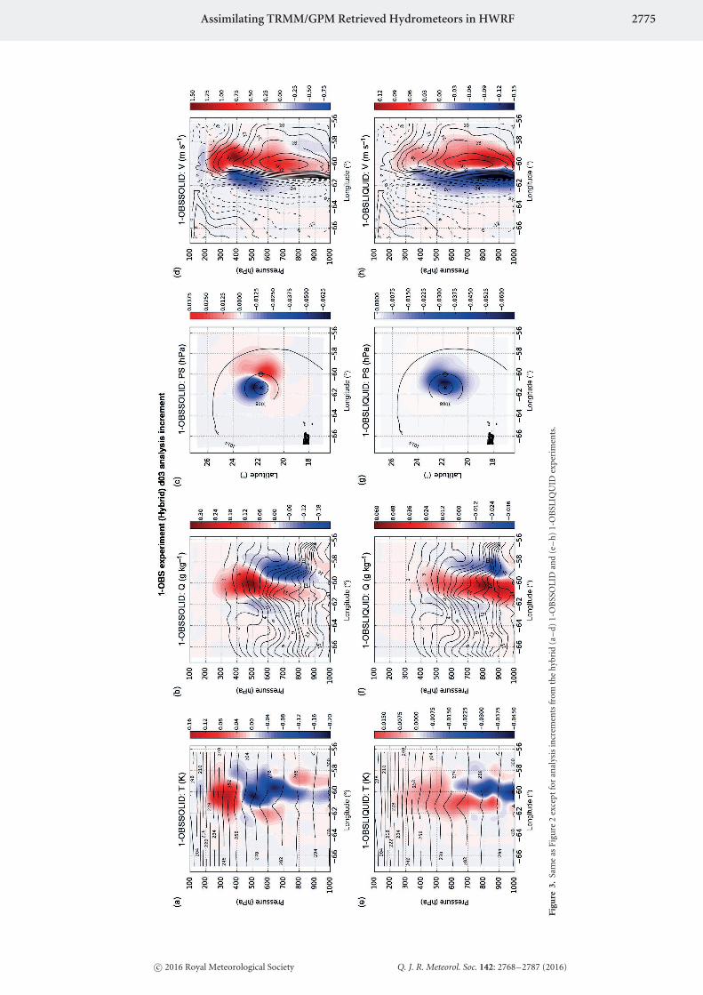
Assimilating TRMM/GPM Retrieved Hydrometeors in HWRF 2775
Figu
re3.
Sam
eas
Figu
re2
exce
ptfo
ran
alys
isin
crem
ents
from
the
hyb
rid
(a–
d)1-
OB
SSO
LID
and
(e–
h)
1-O
BSL
IQU
IDex
peri
men
ts.
c© 2016 Royal Meteorological Society Q. J. R. Meteorol. Soc. 142: 2768–2787 (2016)

2776 T.-C. Wu et al.
Figure 4. GOES-13 visible imagery at (a) 1145 UTC 5 September 2012 duringLeslie, and (b) 1145 UTC 16 October 2014 during Gonzalo.
Table 2. Experimental design for assimilating Hurricane GPROF retrievedintegrated SWC and LWC in the innermost domain of HWRF. WC here denotes
both integrated SWC and integrated LWC.
Experiment Obs Assimilatedin ghost d02
Obs Assimilated inghost d03
Conventional Satellite Conventional Satellite
CTL � � � NoneAddWC � � � WC
Note that for all the AddWC experiments mentioned above, theobservation errors assigned to integrated SWC and LWC are 1.0and 2.0 kg m−2, respectively. These two numbers are estimatesof a root-mean-square deviation from all available HurricaneGPROF retrieved quantities for Leslie and Gonzalo. With thiserror assignment, the ratio of observation errors to the meanvalue of observed quantities is approximately 0.25 for integratedSWC and 0.4 for integrated LWC.
There are a total of six experiments. The first pair of experimentsis conducted for Leslie, hereafter denoted by L1 CTL and L1
Table 3. HWRF forecast experiments for Hurricanes Leslie (2012) and Gonzalo(2014).
Experiments 1st cycle (yyyy/mm/dd hh) 2nd cycle (yyyy/mm/dd hh)
Hurricane Leslie (2012)L1 CTL and AddWC 2012/08/30 1800 UTC 2012/08/31 0000 UTCHurricane Gonzalo (2014)G1 CTL and AddWC 2014/10/13 0000 UTC 2014/10/13 0600 UTCG2 CTL and AddWC 2014/10/16 0600 UTC 2014/10/16 1200 UTC
AddWC. In both L1 experiments, the first cycles begin at 1800UTC 30 August and continue to the second cycles at 0000 UTC31 August. Similarly, a pair of experiments is conducted duringthe observed developing stage of Gonzalo and is denoted by G1CTL and G1 AddWC. In both G1 experiments, the first cyclesbegin at 0000 UTC 13 October and continue to the second cyclesat 0600 UTC on the same day. During the observed maturestage of Gonzalo, the last pair of experiments is conducted andis denoted by G2 CTL and G2 AddWC. Likewise, in both G2experiments, the first cycles begin at 0600 UTC 16 October andcontinue to the second cycles at 1200 UTC on the same day. Theabove-mentioned six experiments are summarized in Table 3.
Since the main difference between the CTL and AddWCexperiments occur in the innermost domain, a discussion of theperformance of the subsequent analysis from the second cycles ofthe six experiments will be specific to d03.
4.3. Results from data assimilation experiments
4.3.1. Observed vs. simulated integrated SWC and LWC
In general, background guessed values of the observed quantitiesare lower, potentially suggesting a negative bias due to the obser-vation operators. An example of the observed integrated SWCand LWC that are assimilated in ghost d03 in the L1 AddWCexperiment is shown in Figure 5(a) and (b). The backgroundguessed values of integrated SWC and LWC and the counter-part from the analysis are illustrated in Figure 5(c), (d), (e)and (f), respectively. Before assimilation, the local maximum val-ues (∼2.5 kg m−2) of the observed integrated SWC (Figure 5(a)),to the southwest quadrant of the storm (magenta star), are foundto be lower in the background (Figure 5(c)). Similar remarks alsoapply to the integrated LWC (Figure 5(b) and (d)). By assimi-lating the observed integrated SWC and LWC together with thenew observation operators, background guessed values of theintegrated SWC and LWC are improved (Figure 5(e) and (f)) andare supported by values of the observed quantities (Figure 5(a)and (b)). When observed quantities for Gonzalo are assimilatedinto the G1 AddWC (Figure 6(a) and (b)) and G2 AddWC (Fig-ure 7(a) and (b)) experiments, favourable results occurred inthat observed quantities support the subsequent analyses. Resultsfrom L1, G1, and G2 AddWC experiments (Figures 5–7) areencouraging as they add confidence of the ability of the newobservation operators (see section 3.3) that serve to modify back-ground state into an analysis state that agrees with observations.Although there is still an indication of the potential bias, theobservation innovation is considerably reduced in the analysis.
4.3.2. Differences between the CTL and AddWC analyses
As a result of the assimilation of retrieved integrated SWCand LWC in ghost d03 (AddWC experiment), the impact ofthe additional observations on the respective analyses (CTLvs. AddWC) is examined. Instead of taking difference betweenthe background and analysis fields of one experiment (analysisincrement, as was done in section 3.3), differences betweenanalyses from the CTL and AddWC experiments are examinedhere. Due to possible asymmetries, in the azimuthal direction, agiven vertical cross-section could contain information that may
c© 2016 Royal Meteorological Society Q. J. R. Meteorol. Soc. 142: 2768–2787 (2016)

Assimilating TRMM/GPM Retrieved Hydrometeors in HWRF 2777
Observation
Background
Analysis
Observation
Background
Analysis
(b)
(d)
(f)
(a)
(c)
(e)
Integrated solid water contents Integrated liquid water contents
Figure 5. Hurricane GPROF retrieved (a) integrated SWC (kg m−2) and (b) integrated LWC (kg m−2) assimilated in the L1 AddWC experiment during Leslie. (c)–(d)Same as (a)–(b) except for background guessed quantities. Similarly, (e)–(f) are estimated quantities from the L1 AddWC analysis. A bold magenta star marks thecentre of Leslie at the analysis time.
or may not be representative of the entire hurricane. To overcomethis issue, azimuthally averaged quantities will be used to showdifferences between the two analyses, following Wu et al. (2014).To aid this analysis, horizontal winds in the rectilinear coordinatesystem (u and v) are converted to radial (V r) and tangential (V t)horizontal winds in a polar coordinate system centred on thehurricane.
Analyses of the L1 CTL and the L1 AddWC and the differences(L1 AddWC minus L1 CTL) are presented in Figure 8. Valuesof azimuthally averaged T, q, V t and V r from the L1 CTLanalysis are shown in Figure 8(a)–(d). Likewise, Figure 8(e)–(h)show the above four variables from the L1 AddWC analysis.To examine the impact of assimilating both retrieved integratedSWC and LWC, differences between the two respective analysesare presented in Figure 8(i)–(l). In Figure 8(i), a local area ofnegative values of T differences between 300 and 800 hPa withinthe first 300 km radius suggests cooler air in the mid-troposphericlayers of the L1 AddWC analysis. Positive values of q difference(Figure 8(j)) are collocated with the negative T differences inFigure 8(i), suggesting cooler air in the mid-tropospheric layers
is accompanied by moister air. Negative values of V t differences(Figure 8(k)) and positive values of V r differences (Figure 8(l))near surface and outside the first 50 km radius imply weakerrotational winds and inflows in the lower tropospheric layersof the L1 AddWC analysis. In contrast, large positive values ofV t differences (Figure 8(k)) and positive values of V r differences(Figure 8(l)) above 300 hPa both suggest stronger rotational windsand outflows in the upper tropospheric layers of the L1 AddWCanalysis. The impact of assimilating both retrieved integratedSWC and LWC in the core region of Leslie on the above-mentioned variables are mixed. Thus, physical interpretations areprecluded. In general, moister and cooler air in the near-coreregion is evident in the mid-tropospheric layers of the L1 AddWCanalysis, suggesting a favourable environment for saturation.Slightly weaker winds in lower, but much stronger upper-layerrotational winds and outflows are also evident in the L1 AddWCanalysis.
Similar to Figure 8, azimuthally averaged quantities from the G1CTL and G1 AddWC analyses and the difference fields are shownin Figure 9. While responses to T are mixed (Figure 9(i)), moister
c© 2016 Royal Meteorological Society Q. J. R. Meteorol. Soc. 142: 2768–2787 (2016)

2778 T.-C. Wu et al.
Observation Observation
Background Background
Analysis Analysis
(kg
m–2
)(k
g m
–2)
(kg
m–2
)
(kg
m–2
)(k
g m
–2)
(kg
m–2
)
(b)
(d)
(f)
(a)
(c)
(e)
Integrated solid water contents Integrated liquid water contents
Figure 6. Same as Figure 5, except for retrieved quantities that are assimilated in the G1 AddWC experiment during Gonzalo.
air throughout the vertical column within the first 100 km radiusis evident in the G1 AddWC analysis (Figure 9(j)). In Figure 9(k)and (l), V t and V r differences both suggest the G1 AddWC analysishas slightly stronger rotational winds throughout the vertical, andalso greater inflows in the lower layer and greater outflows inthe upper layer compared to the G1 CTL analysis. In general,large spatial variability in the difference fields is evident. Such aresponse is expected due to the mixed impact from assimilatingboth retrieved integrated SWC and LWC with the hybrid option(i.e. the operational configuration of GSI in HWRF). Like the1-OBS hybrid experiments, physical interpretation of analysisdifferences is challenging. Since our cases are hurricanes, oneapproach could be to examine the hydrostatic linking of warmertemperatures aloft with lower surface pressures (as was describedin section 3.4) to larger tangential wind speeds through gradientwind balance. However, for the simulations presented herein,azimuthally averaging (e.g. Figures 8 and 9) removes asymmetriesthat are present in the three-dimensional analysis fields. Forbrevity, conclusions from the G2 experiments are similar to G1.
Overall, results from the six experiments are encouraging.By assimilating additional observations in ghost d03 (AddWCexperiments), background guessed values of the integrated SWC
and LWC are adjusted to an analysis state that is supported byobserved quantities. In general, the impact of assimilating bothretrieved integrated water contents causes moister and coolerair in the mid-tropospheric layers to approach saturation whenbackground guess values are lower (e.g. Figures 5–7). Whileresponses to the winds are mixed, results indicated increasedrotational and radial winds in the upper layers.
5. HWRF forecast
A variety of metrics will be used to examine the impact ofassimilating Hurricane GPROF data on HWRF forecasts. Tobegin with, hurricane track, size,¶ and intensity of six forecastsare computed by using the GFDL vortex tracker (Marchok, 2002)package embedded in HWRF. These metrics are then comparedwith the NHC best-track data. Also, simulated precipitation
¶Hurricane size is often described by the maximum extent of winds of 34, 50and 64 kn in each of quadrants about the centre (Landsea and Franklin, 2013).In this study, quadrant-averaged 34 kn wind radius is used as an approximationof hurricane size.
c© 2016 Royal Meteorological Society Q. J. R. Meteorol. Soc. 142: 2768–2787 (2016)

Assimilating TRMM/GPM Retrieved Hydrometeors in HWRF 2779
Observation Observation
Background Background
Analysis Analysis
(kg
m–2
)(k
g m
–2)
(kg
m–2
)
(kg
m–2
)(k
g m
–2)
(kg
m–2
)
(b)
(d)
(f)
(a)
(c)
(e)
Integrated solid water contents Integrated liquid water contents
Figure 7. Same as Figure 6, but for retrieved quantities that are assimilated in the G2 AddWC experiment during Gonzalo.
fields from all six forecasts are compared with rain rates fromthe TRMM and GPM instruments. Finally, synthetic GOES-13 images generated from all six forecasts (using a version ofthe Community Radiative Transfer Model (CRTM) externalto HWRF) are compared with observed GOES-13 images (e.g.Grasso et al., 2014).
5.1. Hurricane track, size, and intensity
Hurricane track, size, minimum central sea-level pressure(MSLP), and maximum 10 m winds (WMAX) from two 126 hHWRF forecasts that are initialized with L1 CTL (blue line) and L1AddWC (green line) analyses are presented in Figure 10. Resultsshow that there is no obvious difference between track forecastsfrom L1 CTL and L1 AddWC (Figure 10(a)). On the other hand,both L1 CTL and L1 AddWC forecasts generate larger storms(∼100 km larger than the NHC best-track data), and remainlarger than the NHC (black line) estimated sizes for the first 36 h(Figure 10(b)). Similarly, the intensity as measured by MSLP andWMAX of the simulated storms from the L1 CTL and the L1AddWC forecasts produce more intense storms than the NHCestimates (Figure 10(c) and (d)). Note in particular that the L1
AddWC forecast, however, intensifies the simulated hurricaneafter the first 72 h and is much different from the L1 CTL forecast.
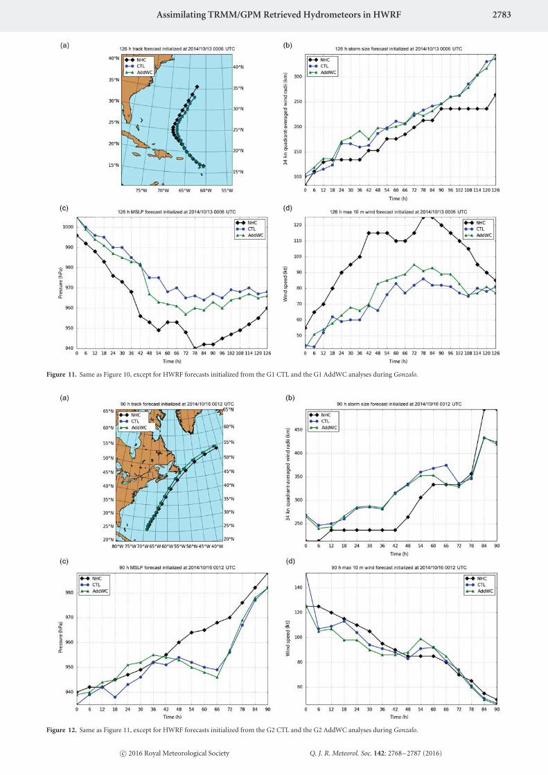
Figure 11 shows results from the G1 CTL (blue line) and the G1AddWC (green line) forecasts. Similar to the L1 Leslie forecasts,Figure 11(a) exhibits no obvious distinction between the G1 CTLand the G1 AddWC track forecasts. In this case, the simulatedstorm sizes from both forecasts are found to be comparable tothe NHC estimated sizes (black line) in the first 18 h of theforecasts (Figure 11(b)). However, the difference in sizes betweenboth G1 forecasts and the NHC estimated sizes is nearly constantwith a value of ∼20 km, indicating slightly larger storm sizesin both forecasts. Unlike the L1 forecasts, values of MSLP andWMAX (Figure 11(c) and (d)) suggest both G1 CTL and G1AddWC forecasts underestimate the intensity of Gonzalo whencompared to the NHC estimates throughout the 126 h period. Itis noteworthy that the G1 AddWC intensity forecast is generallybetter than the G1 CTL intensity forecast.
As for the last pair of forecasts, results from the G2 CTLand G2 AddWC are presented in Figure 12. Both track and sizecomparisons from the G2 CTL and G2 AddWC forecasts exhibitsimilarities to the previous two pairs of forecasts (Figure 12(a)and (b)). Unlike the L1 and G1 pairs of forecasts, the G2 pair of
c© 2016 Royal Meteorological Society Q. J. R. Meteorol. Soc. 142: 2768–2787 (2016)

2780 T.-C. Wu et al.
Figu
re8.
Ver
tica
lpro
file
sof
azim
uth
ally
aver
aged
(a)
tem
pera
ture
(K),
(b)
spec
ific
hu
mid
ity
(gkg
−1),
(c)
tan
gen
tial
win
ds(m
s−1)
and
the
radi
us
ofm
axim
um
win
ds(R
MW
,bla
ckco
nto
ur)
,an
d(d
)ra
dial
win
ds(m
s−1)
from
the
L1C
TL
anal
ysis
duri
ng
Lesl
ie.(
e)–
(h)
Sam
eas
(a)–
(d)
exce
ptfo
rth
eL1
Add
WC
anal
ysis
.(i)
–(l
)ar
edi
ffer
ence
sbe
twee
nth
eL1
CT
Lan
dth
eL1
Add
WC
anal
yses
(L1
Add
CW
min
us
L1C
TL)
.
c© 2016 Royal Meteorological Society Q. J. R. Meteorol. Soc. 142: 2768–2787 (2016)

Assimilating TRMM/GPM Retrieved Hydrometeors in HWRF 2781
Figu
re9.
Sam
eas
Figu
re8,
exce
ptfo
rth
eG
1C
TL
and
the
G1
Add
WC
anal
yses
duri
ng
Gon
zalo
.
c© 2016 Royal Meteorological Society Q. J. R. Meteorol. Soc. 142: 2768–2787 (2016)

2782 T.-C. Wu et al.
Figure 10. The 126 h HWRF forecast (a) track (km), (b) size (km), (c) minimum mean sea-level pressure (hPa), and (d) maximum 10 m winds (kt) initialized fromthe L1 CTL (blue) and the L1 AddWC (green) analyses during Leslie. Black solid lines represent the corresponding estimates from NHC best-track data.
forecasts is initialized at a time when Gonzalo was a hurricane andcovers the time period when the system underwent continuousweakening, underwent extratropical transition (completed on19 October 1800 UTC, 78 h), and eventually dissipated. InFigure 12(c) and (d), the G2 CTL and G2 AddWC forecastsof MSLP are found to be quite similar to the NHC estimatedintensity for the first 48 h. In the rest of the forecast period,MSLP forecasts from both G2 CTL and G2 AddWC exhibitrelatively large deviation from the NHC estimates during theperiod of extratropical transition; however, the correspondingWMAX forecasts are rather similar to the NHC estimatedquantities.
5.2. Precipitation
Simulated precipitation fields from all six forecasts are comparedwith rain rates from TRMM and GPM instruments. For thisstudy, footprint sizes of instantaneous rain rates (mm h−1) fromTRMM at nadir are ∼30 × 20 km2 and ∼4.3 km for TMI and PR,respectively. Similarly, footprint sizes of instantaneous rain rates(mm h−1) from GPM at nadir are ∼16 × 10 km2 and ∼5 km forGMI and DPR, respectively. In addition, d03 is small enoughthat the hurricane rain bands extend beyond the boundary of theinnermost domain; consequently, simulated and observed rainrates will be displayed in d02. Due to the footprint sizes of rainrate data from TRMM/GPM, a comparison of patterns near thecumulus scale is avoided in favour of a qualitative comparison ofpatterns on a larger scale.
Although instantaneous rain rates are unavailable from HWRF,other output variables are used to compare with TRMM/GPM.One such variable is CWM. Following Zhang et al. (2013a),
CWM is integrated over the depth of the simulated domain andis displayed in Figure 13.
Rain rates from TMI/PR that are valid at 1800 UTC 31 August2012 are compared to the column-integrated CWM field (kg m−2;equivalent to mm) from the L1 CTL and the L1 AddWC 18 hforecasts (Figure 13(a)–(c)). Like observations (Figure 13(a)),the majority of the precipitation field is to the south of thecentre of Leslie (bold star) in both the L1 CTL (Figure 13(b))and the L1 AddWC (Figure 13(c)) forecasts. Larger values ofcolumn-integrated CWM to the south of the simulated systemsare reminiscent of convective activity that advects cyclonicallyaround the centre. Similar to the L1 forecasts, the simulatedrain rates from both G1 forecasts exhibit larger values to thenortheast of the centre of Gonzalo (bold star) and are supportedby observed rain rates from GMI/DPR (Figure 13(d)–(f)). Unlikethe spatial patterns exhibited in Figure 13(a)–(f), the regions ofsimulated rain rates encircle the centre of Gonzalo (bold star) inboth observed and simulated fields (Figure 13(g)–(i)). Similarcomparisons between simulated rain rates from HWRF forecastsand retrieved rain rates from the Advanced Microwave SoundingUnit were also examined and showed similar results, but are notshown for the sake of brevity.
5.3. Synthetic satellite images
Due to the lack of available observations over oceans,TRMM/GPM rain rates are supplemented with GOES-13 images.One way to use observed GOES-13 images is through the useof satellite images generated from HWRF outputs (referred toas synthetic satellite images). Synthetic satellite images (Bikoset al., 2012) for all six forecasts are shown along with observed
c© 2016 Royal Meteorological Society Q. J. R. Meteorol. Soc. 142: 2768–2787 (2016)
Assimilating TRMM/GPM Retrieved Hydrometeors in HWRF 2783
Figure 11. Same as Figure 10, except for HWRF forecasts initialized from the G1 CTL and the G1 AddWC analyses during Gonzalo.
Figure 12. Same as Figure 11, except for HWRF forecasts initialized from the G2 CTL and the G2 AddWC analyses during Gonzalo.
c© 2016 Royal Meteorological Society Q. J. R. Meteorol. Soc. 142: 2768–2787 (2016)

2784 T.-C. Wu et al.
(d) (e) (f)
(g) (h) (i)
30 h
18 h
(a) (b) (c)Rain rates CTL (d02) AddWC (d02)
18 h
Figure 13. (a) PR measured (within black lines) and TMI estimated (outside black lines) rain rates (mm h−1 in log scale) and column-integrated CWM (kg m−2 inlog scale) from 18 h HWRF forecasts that are initialized from (b) the L1 CTL and (c) the L1 AddWC analyses during Leslie. (d) DPR measured (within black lines) andGMI estimated (outside black lines) rain rates (mm h−1 in log scale). (e)–(f) Same as (b)–(c), except for 30 h HWRF forecasts that are initialized from the G1 CTLand the G1 AddWC analyses during Gonzalo. Similarly, (g)–(i) are results from 18 h HWRF forecasts that are initialized from the G2 CTL and the G2 AddWC analysesduring Gonzalo. A bold magenta star marks hurricane centre. The unit kg m−2 is equivalent to mm after dividing by density of liquid water, which is 1000 kg m−3.
GOES-13 images at 10.7 μm (Figure 14). In the figure, observedand synthetic GOES-13 imagery from the L1 CTL and the L1AddWC forecasts are shown in Figure 14(a)–(c); imagery fromthe G1 CTL and the G1 AddWC forecasts are exhibited inFigure 14(d)–(f); and results from the final pair are displayedin Figure 14(g)–(i). All synthetic images are generated with theCRTM and brightness temperatures are sensitive to particle sizes.For this study, the particle size of ice is set to 75 μm, a size that isconsistent with particle sizes of ice in GSI.
In general, the area within the dash boxes of the syntheticimages that is occupied by cold clouds (<−60 ◦C) is larger thanthe corresponding area in the observed images. These cold biasesare particularly evident in the coldest cloud tops with HWRFforecasts having nearly twice as much area being covered bycloud tops colder than −70 ◦C. It is interesting to note thatas the temperature threshold is increased to −40 ◦C the arealcoverage in HWRF is more comparable and actually slightlysmaller than the observations. This may be suggesting that theconvective vertical motions are overactive in HWRF or otherissues related to microphysics. Additionally, these findings areconsistent with observational studies relating infrared imagery totropical cyclone wind structures (Knaff et al., 2014, 2016) and the
results presented in section 5.1, in which a larger and more intensetropical system is found in both L1 CTL and L1 AddWC forecasts.Finally, it is also noteworthy that the assimilation of retrievedintegrated SWC and LWC from TRMM/GPM provides slightlyimproved initial conditions in terms of the observed GOES-13imagery.
6. Summary and discussion
The GSI capability of assimilating satellite-retrieved integratedSWC and LWC from Hurricane GPROF in HWRF is developedand assessed in this study. To assimilate the retrieved integratedwater contents, new observation operators are developed andimplemented in GSI. The concept behind the development ofthe new observation operators assumes all water vapour in excessof saturation with respect to ice or liquid will be immediatelycondensed out. Without introducing new control variables intoGSI, the new observation operators are implemented in such away that the information of integrated water contents is extendedto some – temperature, specific humidity and pressure – of thecurrent set of GSI control variables.
c© 2016 Royal Meteorological Society Q. J. R. Meteorol. Soc. 142: 2768–2787 (2016)

Assimilating TRMM/GPM Retrieved Hydrometeors in HWRF 2785
Figure 14. (a) GOES-13 10.7 μm infrared imagery and the corresponding synthetic satellite images (brightness temperature in ◦ C) from 6 h HWRF forecasts thatare initialized from (b) the L1 CTL and (c) the L1 AddWC analyses during Leslie. Regions of interest, d03 of HWRF, are shown in the dash box. (d)–(f) Same as(a)–(c) except for 6 h HWRF forecasts that are initialized from the G1 CTL and the G1 AddWC analyses during Gonzalo. Similarly, (g)–(i) are results from 6 h HWRFforecasts that are initialized from the G2 CTL and the G2 AddCW analyses during Gonzalo. A bold magenta star marks hurricane centre in the GOES-13 image.
Two 1-OBS experiments that use the no-hybrid option areconducted to assimilate a single integrated SWC and a singleintegrated LWC both of which are for a hurricane environment.Both no-hybrid experiments suggest that the new observationoperators are capable of extending information from integratedSWC and integrated LWC into nearby grid points and other statevariables in a physically consistent way. In particular, a concisephysical interpretation is provided to explain analysis incrementsin temperature, specific humidity and surface pressure from theno-hybrid 1-OBS experiments. Results from the correspondingexperiments that are conducted with a hybrid option exhibit morespatial variability because of the inclusion of flow-dependentbackground error covariance that originates from GFS ensembleforecasts. Due to the variability in the hybrid 1-OBS experiments,a physical interpretation is less straightforward. Nevertheless,analysis increments from the above-mentioned state variablesexhibit consistent adjustment from a background state to ananalysis.
Two hurricanes, Leslie (2012) and Gonzalo (2014), are selectedto perform three sets of two data assimilation experiments withthe use of the retrieved integrated SWC and LWC within HWRF.A CTL experiment, following the current operational HWRFimplementation, and an AddWC experiment that assimilates
Hurricane GPROF retrieved integrated SWC and LWC togetheralong with conventional observations in the innermost domainare conducted. In general, moister and cooler air in mid tolower tropospheric layers of the hurricane core are evident inthe AddWC analysis, suggesting a tendency toward reachingsaturation by lowering temperature and increasing moisture.Tangential and radial winds resolved in the AddWC analysis areslightly more intense in the mid to upper tropospheric layers,near the hurricane core, compared to the CTL analysis.
Although ‘all water vapour in excess of the saturationis immediately condensed out’ is a valid assumption, themodel microphysics and/or cumulus parametrization has alreadycondensed out a portion of supersaturated water vapour. As aresult, the supersaturation computed by the observation operatorsis likely reduced, therefore potentially creating a negative bias ofthe guess. A possible remedy for this issue will be to introduce/adda model variable in HWRF to retain an adequate amount ofexcessive water vapour. Nevertheless, the results indicate thatthe system is still able to considerably reduce the observationinnovation in the analysis.
In general, the impact of assimilating the TRMM/GPMprecipitation observations (integrated SWC and integrated LWC)in the innermost domain on the HWRF forecasts is inconclusive.
c© 2016 Royal Meteorological Society Q. J. R. Meteorol. Soc. 142: 2768–2787 (2016)

2786 T.-C. Wu et al.
Both the CTL and the AddWC forecasts generate larger hurricanescompared to observations. However, the impact on the AddWCforecasts was to produce lower MSLP and greater WMAX attimes. Comparisons between both the CTL and the AddWCforecasts to TRMM/GPM rain rates suggest that the simulatedprecipitation fields are not only similar between the two forecasts,but also comparable to observations. The synthetic satelliteimages generated from the CTL and the AddWC forecastsexhibit similar characteristics. However, issues in the syntheticimages are identified from a comparison between synthetic andobserved GOES-13 images. These issues include (i) colder cloud-top brightness temperatures and (ii) larger spatial extension ofcold brightness temperatures, both in the vicinity of the simulatedtropical storms. A few possible causes of the inconclusive natureof our results are the following: (i) the analysis used to initialize anHWRF forecast is unbalanced, (ii) the existence of forecast modelerrors (e.g. errors in microphysics parametrization schemes) thatare not accounted for by the HWRF data assimilation system, and(iii) the absence of hydrometeor variables in the list of operationalGSI control variables.
A few different approaches will be explored in future work. Inthis study, a retrieved quantity was assimilated and the impact onHWRF forecasts was inconclusive. A statistical inference about theimpact on the general population of experiments where retrievedprecipitation observations are assimilated into HWRF requiresmore experiments than the two presented here (i.e. sample sizeis too small). Long-term efforts will extend current work byconducting similar experiments with more hurricane cases andalso explore the feasibility of assimilating all-sky satellite radiancesdirectly into HWRF.
Acknowledgements
This research is primarily funded by NOAA’s Sandy SupplementalAward NA14OAR4830122. We would like to acknowledgethe high-performance computing support from Yellowstoneprovided by NCAR’s Computational and Information SystemsLaboratory, sponsored by the National Science Foundation. Theviews, opinions, and findings in this report are those of theauthors, and should not be construed as an official NOAA and/orUS Government position, policy, or decision. The authors aregrateful to the two anonymous reviewers for their careful reviewsand valuable comments.
Appendix
Jacobians for integrated SWC and integrated LWC operators
The derivatives of the integrated SWC and/or integrated LWCoperator with respect to T, P and q, also known as Jacobians, arealso calculated. From Eqs (1)–(9), the operator at each modelvertical level k can be rewritten as
hk ={(
qk
1 − qk
)− 0.622
es(Tk)
Pk − es(Tk)
}ρk�zk (A1)
using the same notations. Since ρk�zk is equivalent to �Pk
g
according to the hydrostatic equation and ideal gas law, Eq. (A1)can be written as
hk ={(
qk
1 − qk
)− 0.622
es(Tk)
Pk − es(Tk)
}�Pk
g. (A2)
For simplicity, the vertical index k is dropped, and the operatorat each model vertical level can then be expressed by
h ={(
q
1 − q
)− 0.622
es(T)
P − es(T)
}�P
g(A3)
as a function of T, P and q: h = f (T, P, q).The corresponding tangent linear and adjoint operators are a
linear combination of perturbations of T, P and q:
δh = ∂h
∂TδT + ∂h
∂PδP + ∂h
∂qδq, (A4)
where δh represents the increments of integrated SWC orintegrated LWC, and δT, δP and δq are the perturbations ofT, P and q, respectively. Similarly, ∂h
∂T , ∂h∂P and ∂h
∂q are the Jacobians
with respect to T, P and q. Based on the approximate calculationof derivatives of �P
g with respect to T, P and q, it is assumed
that these derivatives are negligible compared to the derivatives of(q
1−q
)− 0.622 es(T)
P−es(T) with respect to T, P and q. The Jacobians
can then be written as below:
∂h
∂T= −0.622
P
(P − es)2
∂es
∂T
�P
g, (A5a)
∂h
∂P= 0.622
es
(P − es)2
�P
g, (A5b)
∂h
∂q= 1
(1 − q)2
�P
g. (A5c)
In Eq. (A5a),
∂es
∂T= esl
∂w
∂T+ w
∂esl
∂T− esi
∂w
∂T+ (1 − w)
∂esi
∂T, (A6)
where
∂w
∂T= 2
1
cosh2(�T)
(1
T0 − Tmix
), (A7)
∂esl
∂T= esl
(−C
liquid1
T+ C
liquid2 · T0
T2
), (A8)
and
∂esi
∂T= esi
(−Cice1
T+ Cice
2 · T0
T2
). (A9)
The above equations are implemented in GSI.
References
Bernardet L, Tallapragada V, Bao S, Trahan S, Kwon Y, Liu Q, TongM, Biswas M, Brown T, Stark D, Carson L, Yablonsky R, Uhlhorn E,Gopalakrishnan S, Zhang X, Marchok T, Kuo B, Gall R. 2015. Communitysupport and transition of research to operations for the Hurricane WeatherResearch and Forecasting model. Bull. Am. Meteorol. Soc. 96: 953–960, doi:10.1175/BAMS-D-13-00093.1.
Bikos D, Lindsey DT, Otkin J, Sieglaff J, Grasso L, Siewart C, Correia J,Coniglio M, Rabin R, Kain JS, Dembek S. 2012. Synthetic satellite imageryfor real-time high-resolution model evaluation. Weather and Forecasting 27:784–795, doi: 10.1175/WAF-D-11-00130.1.
Brown DP. 2015. ‘Hurricane Gonzalo (AL082014): 12–19 October 2014’,National Hurricane Center Tropical Cyclone report. www.nhc.noaa.gov/data/tcr/AL082014_Gonzalo.pdf (accessed 15 August 2016).
Brown PJ, Kummerow CD, Randel DL. 2016. Hurricane GPROF: An optimizedocean microwave rainfall retrieval for tropical cyclones. J. Atmos. OceanicTechnol. 33: 1539–1556, doi: 10.1175/JTECH-D-15-0234.1.
Chambon P, Zhang SQ, Hou AY, Zupanski M, Cheung S. 2014. Assessing theimpact of pre-GPM microwave precipitation observations in the GoddardWRF ensemble data assimilation system. Q. J. R. Meteorol. Soc. 140:1219–1235, doi: 10.1002/qj.2215.
Cotton WR. 1972. Numerical simulation of precipitation development insupercooled cumuli – Part II. Mon. Weather Rev. 100: 764–784, doi:10.1175/1520-0493(1972)100<0764:NSOPDI>2.3.CO;2.
c© 2016 Royal Meteorological Society Q. J. R. Meteorol. Soc. 142: 2768–2787 (2016)

Assimilating TRMM/GPM Retrieved Hydrometeors in HWRF 2787
Emanuel KA. 1994. Atmospheric Convection. Oxford University Press: NewYork, NY.
Ferrier BS. 2005. An efficient mixed-phase cloud and precipitation scheme foruse in operational NWP models. Eos. Trans. Am. Geophys. Union 86 Jt.Assem. Suppl.: A42A02.
Grasso L, Lindsey DT, Lim K-SS, Clark A, Bikos D, Dembek SR. 2014.Evaluation of and suggested improvements to the WSM6 microphysics inWRF-ARW using synthetic and observed GOES-13 imagery. Mon. WeatherRev. 142: 3635–3650, doi: 10.1175/MWR-D-14-00005.1.
Hence DA, Houze RA Jr. 2012. Vertical structure of tropical cyclone rainbandsas seen by the TRMM precipitation radar. J. Atmos. Sci. 69: 2644–2661, doi:10.1175/JAS-D-11-0323.1.
Hou AY, Zhang SQ, Reale O. 2004. Variational continuous assimilationof TMI and SSM/I rain rates: Impact on GEOS-3 hurricane analysesand forecasts. Mon. Weather Rev. 132: 2094–2109, doi: 10.1175/1520-0493(2004)132<2094:VCAOTA>2.0.CO;2.
Hou AY, Kakar RK, Neeck S, Azarbarzin AA, Kummerow CD, Kojima M,Oki R, Nakamura K, Iguchi T. 2014. The global precipitation measurementmission. Bull. Am. Meteorol. Soc. 95: 701–722, doi: 10.1175/BAMS-D-13-00164.1.
Iguchi T, Kozu T, Meneghini R, Awaka J, Okamoto K. 2000. Rain-profilingalgorithm for the TRMM precipitation radar. J. Appl. Meteorol. 39:2038–2052, doi: 10.1175/1520-0450(2001)040<2038:RPAFTT>2.0.CO;2.
Janjic ZI. 2003. A nonhydrostatic model based on a new approach. Meteorol.Atmos. Phys. 82: 271–285, doi: 10.1007/s00703-001-0587-6.
Kleist DT, Parrish DF, Derber JC, Treadon R, Wu W-S, Lord S. 2009.Introduction of the GSI into the NCEP Global Data Assimilation System.Weather Forecasting 24: 1691–1705, doi: 10.1175/2009WAF2222201.1.
Knaff JA, Longmore SP, Molenar DA. 2014. An objective satellite-basedtropical cyclone size climatology. J. Clim. 27: 455–476, doi: 10.1175/JCLI-D-13-00096.1.
Knaff JA, Slocum CJ, Musgrave KD, Sampson CR, Strahl BR. 2016. Usingroutinely available information to estimate tropical cyclone wind structure.Mon. Weather Rev. 144: 1233–1247, doi: 10.1175/MWR-D-15-0267.1.
Kumar P, Kishtawal CM, Pal PK. 2014. Impact of satellite rainfall assimilationon Weather Research and Forecasting model predictions over the Indianregion. J. Geophys. Res. Atmos. 119: 2017–2031, doi: 10.1002/2013JD020005.
Kummerow CD, Barnes W, Kozu T, Shiue J, Simpson J. 1998. TheTropical Rainfall Measuring Mission (TRMM) sensor package. J. Atmos.Oceanic Technol. 15: 809–817, doi: 10.1175/1520-0426(1998)015<0809:TTRMMT>2.0.CO;2.
Kummerow CD, Hong Y, Olson WS, Yang S, Adler RF, McCollum J,Ferraro R, Petty G, Shin D-B, Wilheit TT. 2001. The evolution of theGoddard Profiling algorithm (GPROF) for rainfall estimation from passivemicrowave sensors. J. Appl. Meteorol. 40: 1801–1820, doi: 10.1175/1520-0450(2001)040<1801:TEOTGP>2.0.CO;2.
Kummerow CD, Randel DL, Kulie M, Wang N-Y, Ferraro R, Munchak SJ,Petkovic V. 2015. The evolution of the Goddard Profiling algorithm to afully parametric scheme. J. Atmos. Oceanic Technol. 32: 2265–2280, doi:10.1175/JTECH-D-15-0039.1.
Landsea CW, Franklin JL. 2013. Atlantic hurricane database uncertainty andpresentation of a new database format. Mon. Weather Rev. 141: 3576–3592,doi: 10.1175/MWR-D-12-00254.1.
Lorenc AC, Rawlins F. 2005. Why does 4D-Var beat 3D-Var? Q. J. R. Meteorol.Soc. 131: 3247–3257, doi: 10.1256/qj.05.85.
Marchok TP. 2002. ‘How the NCEP tropical cyclone tracker works’. InPreprints, 25th Conference on Hurricanes and Tropical Meteorology, AmericanMeteorological Society. San Diego, CA, pp. 21-22.
Morrison H, Curry JA, Shupe MD, Zuidema P. 2005. A new double-momentmicrophysics parameterization for application in cloud and climate models.Part II: Single-column modeling of Arctic clouds. J. Atmos. Sci. 62:1678–1693, doi: 10.1175/JAS3447.1.
National Oceanic and Atmospheric Administration. 2010. ‘NOAA’s nextgeneration strategic plan, 2009–2014’. http://www.ppi.noaa.gov/ngsp/(accessed 15 August 2016).
Parrish DF, Derber JC. 1992. The National Meteorological Center’s spectralstatistical-interpolation analysis system. Mon. Weather Rev. 120: 1747–1763,doi: 10.1175/1520-0493(1992)120<1747:TNMCSS>2.0.CO;2.
Pu ZX, Tao W-K, Braun S, Simpson J, Jia YQ, Halverson J, Olson W, HouA. 2002. The impact of TRMM data on mesoscale numerical simulation ofSupertyphoon Paka. Mon. Weather Rev. 130: 2448–2458.
Purser RJ, Wu W-S, Parrish DF, Roberts NM. 2003. Numericalaspects of the application of recursive filters to variational statisti-cal analysis. Part I: Spatially homogeneous and isotropic Gaussiancovariances. Mon. Weather Rev. 131: 1524–1535, doi: 10.1175//1520-0493(2003)131<1524:NAOTAO>2.0.CO;2.
Rappaport EN, Franklin JL, Avila LA, Baig SR, Beven JL, Blake ES, Burr CA,Jiing J-G, Juckins CA, Knabb RD, Landsea CW, Mainelli M, Mayfield M,McAdie CJ, Pasch RJ, Sisko C, Stewart SR, Tribble AN. 2009. Advances andchallenges at the National Hurricane Center. Weather and Forecasting 24:395–419, doi: 10.1175/2008WAF2222128.1.
Simpson J, Kummerow CD, Tao W-K, Adler RF. 1996. On the tropicalrainfall measuring mission (TRMM). Meteorol. Atmos. Phys. 60: 19–36, doi:10.1007/BF01029783.
Stewart SR. 2013. Hurricane Leslie (AL122012) 30 August – 11 September 2012.Tropical Cyclone report. National Hurricane Center: Miami, FL. http://www.nhc.noaa.gov/data/tcr/AL122012_Leslie.pdf (accessed 15 August 2016).
Tallapragada V, Bernadet L, Biswas MK, Gopalakrishnan S, Kwon Y, Liu Q,Marchok T, Sheinin D, Tong M, Trahan S, Tuleya R, Yablonsky R, ZhangX. 2014. Hurricane Weather Research and Forecasting (HWRF) Model: 2014Scientific Documentation. Developmental Testbed Center: Boulder, CO.
Tallapragada V, Bernadet L, Biswas MK, Ginis I, Kwon Y, Liu Q,Marchok T, Sheinin D, Thomas B, Tong M, Trahan S, Wang W,Yablonsky R, Zhang X. 2015. ‘Hurricane Weather Research and Forecasting(HWRF) Model: 2015 scientific documentation’, NCAR Technical NoteNCAR/TN-522+STR. NCAR/UCAR: Boulder, CO. http://nldr.library.ucar.edu/collections/technotes/TECH-NOTE-000-000-000-893.pdf (accessed15 August 2016).
Thompson G, Rasmussen RM, Manning K. 2004. Explicit forecasts ofwinter precipitation using an improved bulk microphysics scheme. PartI: Description and sensitivity analysis. Mon. Weather Rev. 132: 519–542,doi: 10.1175/1520-0493(2004)132<0519:EFOWPU>2.0.CO;2.
Wang X. 2010. Incorporating ensemble covariance in the Gridpoint StatisticalInterpolation variational minimization: a mathematical framework. Mon.Weather Rev. 138: 2990–2995, doi: 10.1175/2010MWR3245.1.
Wu W-S, Purser RJ, Parrish DF. 2002. Three-dimensional variationalanalysis with spatially inhomogeneous covariances. Mon. Weather Rev. 130:2905–2916, doi: 10.1175/1520-0493(2002)130<2905:TDVAWS>2.0.CO;2.
Wu T-C, Liu H, Majumdar SJ, Velden CS, Anderson JL. 2014. Influence ofassimilating satellite-derived atmospheric motion vector observations onnumerical analyses and forecasts of tropical cyclone track and intensity.Mon. Weather Rev. 142: 49–71, doi: 10.1175/MWR-D-13-00023.1.
Yablonsky RM, Ginis I, Thomas B, Tallapragada V, Sheinin D, BernardetL. 2015. Description and analysis of the ocean component of NOAA’soperational Hurricane Weather Research and Forecasting model (HWRF).J. Atmos. Oceanic Technol. 32: 144–163, doi: 10.1175/JTECH-D-14-00063.1.
Yu H, Marchok T, Woo W-C. 2014. ‘Topic 8: Rainfall’. In WMO’s ThirdInternational Workshop on Tropical Cyclone Landfall Processes, 8–10December 2014. Jeju, Republic of Korea. http://www.wmo.int/pages/prog/arep/wwrp/new/documents/C_T8.pdf (accessed 15 August 2016).
Zhang M, Zupanski M, Kim M-J, Knaff JA. 2013a. Assimilating AMSU-Aradiances in the TC core area with NOAA operational HWRF (2011) anda hybrid data assimilation system: Danielle (2010). Mon. Weather Rev. 141:3889–3907, doi: 10.1175/MWR-D-12-00340.1.
Zhang SQ, Zupanski M, Hou AY, Lin X, Cheung SH. 2013b. Assimilation ofprecipitation-affected radiances in a cloud-resolving WRF ensemble dataassimilation system. Mon. Weather Rev. 141: 754–772, doi: 10.1175/MWR-D-12-00055.1..
Zupanski D. 1993. The effects of discontinuities in the Betts–Miller cumulusconvection scheme on four-dimensional variational data assimilation. TellusA 45: 511–524, doi: 10.3402/tellusa.v45i5.15053.
Zupanski D, Zhang SQ, Zupanski M, Hou AY, Cheung SH. 2011. A prototypeWRF-based ensemble data assimilation system for dynamically downscalingsatellite precipitation observations. J. Hydrometeorol. 12: 118–134, doi:10.1175/2010JHM1271.1.
c© 2016 Royal Meteorological Society Q. J. R. Meteorol. Soc. 142: 2768–2787 (2016)


![TRMM Key TRMM Facts - NASA · 244 [ Missions: TRMM ] Earth Science Reference Handbook TRMM Science Goals • Obtain and study multiyear science data sets of tropical and subtropical](https://static.fdocuments.net/doc/165x107/5edb4b20ad6a402d66657010/trmm-key-trmm-facts-nasa-244-missions-trmm-earth-science-reference-handbook.jpg)