
The Growth and Enrichment of the Intragroup Gas by Lichen ...
139
The Growth and Enrichment of the Intragroup Gas by Lichen Liang B.Sc., Zhejiang University, 2011 A Thesis Submitted in Partial Fulfillment of the Requirements for the Degree of MASTER OF SCIENCE in the Department of Physics and Astronomy c Lichen Liang, 2015 University of Victoria All rights reserved. This thesis may not be reproduced in whole or in part, by photocopying or other means, without the permission of the author.
Transcript of The Growth and Enrichment of the Intragroup Gas by Lichen ...

The Growth and Enrichment of the Intragroup Gas
by
Lichen Liang
B.Sc., Zhejiang University, 2011
A Thesis Submitted in Partial Fulfillment of the
Requirements for the Degree of
MASTER OF SCIENCE
in the Department of Physics and Astronomy
c© Lichen Liang, 2015
University of Victoria
All rights reserved. This thesis may not be reproduced in whole or in part, by
photocopying or other means, without the permission of the author.

ii
The Growth and Enrichment of the Intragroup Gas
by
Lichen Liang
B.Sc., Zhejiang University, 2011
Supervisory Committee
Dr. Arif Babul, Supervisor
(Department of Physics and Astronomy)
Dr. Christopher Pritchet, Departmental Member
(Department of Physics and Astronomy)
Dr. Alexandre Brolo, Outside Member
(Department of Chemistry)

iii
Supervisory Committee
Dr. Arif Babul, Supervisor
(Department of Physics and Astronomy)
Dr. Christopher Pritchet, Departmental Member
(Department of Physics and Astronomy)
Dr. Alexandre Brolo, Outside Member
(Department of Chemistry)
ABSTRACT
The observable properties of galaxy groups, and especially the thermal and chem-
ical properties of the intragroup medium (IGrM), provide important constraints on
the different feedback processes associated with massive galaxy formation and evolu-
tion. In this work, we present a detailed analysis of the global properties of simulated
galaxy groups with X-ray temperatures in the range 0.5 − 2 keV over the redshift
range 0 ≤ z ≤ 3. The groups are drawn from a cosmological smoothed particle hy-
drodynamics simulation that includes a well-constrained prescription for momentum-
driven, galactic outflows powered by stars and supernovae but no explicit treatment
of AGN feedback. Our aims are (a) to establish a baseline against which we will
compare future models; (b) to identify model successes that are genuinely due to
stellar/supernovae-powered outflows; and (c) to pinpoint mismatches that not only
signal the need for AGN feedback but also constrain the nature of this feedback.
We find that even without AGN feedback, our simulation successfully reproduces
the observed present-day group properties such as the IGrM mass fraction, the various
X-ray luminosity-temperature-entropy scaling relations, as well as both the mass-
weighted and the emission-weighted IGrM iron and silicon abundance versus IGrM
temperature relationships, for all but the most massive groups. We also show that
these trends evolve self-similarly for z < 1, in agreement with the observations. In

iv
contrast to the usual expectations, we do not see any evidence of the IGrM undergoing
catastrophic cooling. And yet, the z = 0 group stellar mass is a factor of ∼ 2 too
high. Probing further, we find that the latter is due to the build-up of cold gas in the
massive galaxies before they are incorporated inside groups. This not only indicates
that another feedback mechanism must activate as soon as the galaxies achieve M∗ ≈a few ×1010 M but that this feedback mechanism must be powerful enough to expel a
significant fraction of the halo gas component from the galactic halos. “Maintenance-
mode” AGN feedback of the kind observed in galaxy clusters will not do. At the same
time, we find that stellar/supernovae-powered winds are essential for understanding
the metal abundances in the IGrM and these results are expected to be relatively
insensitive to the addition of AGN feedback.
We further examine the detailed distribution of the metals within the groups and
their origin. We find that our simulated abundance profiles fit the observational data
pretty well except that in the innermost regions, there appears to have an excess of
metals in the IGrM, which is attributed to the overproduction of stars in the central
galaxies. The fractional contribution of the different types of galaxies varies with
radial distances from the group center. While the enrichment in the core regions of
the groups is dominated by the central and satellite galaxies, the external galaxies
become more important contributors to the metals at r >∼ R500. The IGrM at the
groups’ outskirts is enriched at comparatively higher redshifts, and by relatively less
massive galaxies.

v
Contents
Supervisory Committee ii
Abstract iii
Table of Contents v
List of Figures vii
Acronyms xvi
Acknowledgements xviii
Dedication xx
1 INTRODUCTION 1
1.1 The Cosmology . . . . . . . . . . . . . . . . . . . . . . . . . . . . . . 1
1.2 Groups and Clusters . . . . . . . . . . . . . . . . . . . . . . . . . . . 7
1.3 This Work . . . . . . . . . . . . . . . . . . . . . . . . . . . . . . . . . 15
1.3.1 The Stellar-powered Outflow . . . . . . . . . . . . . . . . . . . 15
1.3.2 Thesis layout . . . . . . . . . . . . . . . . . . . . . . . . . . . 18
2 SIMULATING GALAXY GROUPS 20
2.1 Simulation Details . . . . . . . . . . . . . . . . . . . . . . . . . . . . 20
2.2 Finding Galaxies and Galaxy Groups in the Simulation Volume . . . 23
2.3 Computing Group Properties . . . . . . . . . . . . . . . . . . . . . . 27
3 THE SIMULATED PROPERTIES OF THE IGRM 32
3.1 GLOBAL X-RAY PROPERTIES OF GALAXY GROUPS . . . . . . 32
3.1.1 The Mass-Luminosity-Temperature Scaling Relations . . . . . 33
3.1.2 The Entropy-Temperature Scaling . . . . . . . . . . . . . . . . 40

vi
3.2 THE BARYON CONTENT OF GALAXY GROUPS . . . 44
3.2.1 Stellar, Gas and Total Baryon Fractions . . . . . . . . . . . . 44
3.2.2 Assembly of the Present-day Groups . . . . . . . . . . . . . . 57
3.3 METAL ENRICHMENT OF THE INTRAGROUP MEDIUM . . . . 60
3.3.1 The metallicity of the IGrM . . . . . . . . . . . . . . . . . . . 62
3.3.2 Sources of the IGrM Metals . . . . . . . . . . . . . . . . . . . 64
3.3.3 Abundance Ratios in the IGrM . . . . . . . . . . . . . . . . . 66
3.3.4 The Characteristic Timescales for Metal Enrichment of the IGrM 68
3.4 SUMMARY AND CONCLUSIONS . . . . . . . . . . . . . . . . . . . 71
4 THE ENRICHMENT OF THE IGRM - HOW? WHERE? WHEN?
75
4.1 Radial profiles . . . . . . . . . . . . . . . . . . . . . . . . . . . . . . . 75
4.1.1 Abundance Profiles at present . . . . . . . . . . . . . . . . . . 77
4.1.2 The evolution of metal profiles . . . . . . . . . . . . . . . . . . 79
4.2 Dissecting the enrichment of the IGrM . . . . . . . . . . . . . . . . . 82
4.2.1 The origin of the IGrM metals . . . . . . . . . . . . . . . . . . 82
4.2.2 Where and when was the gas enriched/ejected? . . . . . . . . 93
4.3 Conclusions . . . . . . . . . . . . . . . . . . . . . . . . . . . . . . . . 98
5 SUMMARY AND FUTURE OUTLOOK 101
Bibliography 107

vii
List of Figures
Figure 2.1 The mass function of halos with at least three (red), two (blue),
one (magenta) luminous galaxies, as well as of the complete halo
population in the simulation volume (black) described in Sec-
tion 2.2. The dashed vertical line shows our halo mass resolution
limit of 2.7× 10¹⁰M, corresponding to 64 dark matter particles. 24
Figure 2.2 The top panel shows the z = 0 galaxy stellar mass function
(GSMF) of all luminous galaxies in the simulated groups, sorted
into three mass bins: 12.5 < log Mvir ≤ 13.0 M (magenta),
13.0 < log Mvir ≤ 13.2 M (blue), and 13.2 < log Mvir ≤14.0 M (red). For comparative purposes, we also plot as con-
nected black squares the GSMF for X-ray detected low mass
groups spanning the mass range similar to that of our simu-
lated groups (Giodini et al., 2012). The vertical dashed black
line shows our luminous galaxy stellar mass resolution limit (see
text). In anticipation of the discussion in §3.2.1, the lower panel
shows the same GSMFs as in the top except that the stellar
mass of galaxies in the simulation with M∗ > 1011M has been
artificially reduced by a factor of 3. . . . . . . . . . . . . . . . 25
Figure 2.3 Mvir−TX relation of galaxy groups with at least three (red) and
two (blue) luminous galaxies. TX is tightly correlated with Mvir
and follows the scaling relation: Mvir ∝ T 1.7X . Groups that lie
significantly off this relationship are located near larger systems
and are “contaminated” by the latters’ hot diffuse gas. Excluding
groups with fewer than three luminous galaxies, eliminates most
of these “contaminated” halos. . . . . . . . . . . . . . . . . . . 30

viii
Figure 3.1 X-ray luminosity−T relation for simulated groups at z = 0
(black), z = 0.5 (blue), and z = 1 (red), z = 2 (green), and
z = 3 (cyan). The solid lines show the scaling relationship be-
tween the X-ray luminosity that is emitted by gas within R500
and the core-corrected spectroscopic temperature. The error bars
indicate 1-σ scatter. The dotted and the dashed curves show the
mean LX − T for the z = 0 simulated groups, where T is the
mass-weighted and emission-weighted temperature (both core-
corrected), respectively. Squares, stars and triangles show ob-
served low redshift group data from Osmond & Ponman (2004),
Pratt et al. (2009) and Eckmiller, Hudson & Reiprich (2011), re-
spectively. We plot all the groups in Osmond & Ponman (2004)
including those with a small radial extent in observable X-rays
(i.e. their H sample). Luminosity in the Pratt et al. (2009) and
Eckmiller, Hudson & Reiprich (2011) data is corrected to the
0.5− 2 keV band. . . . . . . . . . . . . . . . . . . . . . . . . . 34
Figure 3.2 LX −M relation for simulated groups at z = 0 (black), z = 0.5
(blue), z = 1 (red), z = 2 (green), and z = 3 (cyan). The error
bars show 1-σ scatter. The circles, stars and squares show data
from Eckmiller, Hudson & Reiprich (2011), Pratt et al. (2009),
and Lagana, de Souza & Keller (2010), respectively. The hydro-
static mass estimates from the first two studies have been cor-
rected for the hydrostatic bias (Haines et al., 2015) and LX,bol
from Pratt et al. (2009) have been converted to LX,0.1−2.4 keV.
We also convert the weak-lensing M200 values from Lagana, de
Souza & Keller (2010) to M500 using an NFW profile,2 and we
scale their luminosities using the median value of LX,0.1−2.4 keV(<
R200)/LX,0.1−2.4 keV(< R500) for our simulated groups. The ob-
served groups at z ≤ 0.25, 0.25 < z ≤ 0.75, and z > 0.75 are
plotted as black, blue and red symbols, respectively. . . . . . . 35

ix
Figure 3.3 M − Tspec,corr relation for simulated groups at z = 0 (black),
z = 0.5 (blue), z = 1 (red), z = 2 (green), and z = 3 (cyan).
The error bars show 1-σ scatter. The black squares and triangles
show the results from Sun et al. (2009) and Eckmiller, Hudson &
Reiprich (2011). The hydrostatic mass estimates given in these
two studies have been corrected for the hydrostatic bias (Haines
et al., 2015). We also note that the temperatures in the lat-
ter study are not always extracted in a consistent, systematic
fashion. The diamonds show results from Kettula et al. (2013);
their masses are weak-lensing estimates. The observed groups
at z ≤ 0.25 and 0.25 < z ≤ 0.75 are plotted as black and blue
symbols, respectively. . . . . . . . . . . . . . . . . . . . . . . . 39
Figure 3.4 Gas entropy at R500 (top panel) and R2500 (bottom panel) of
the simulated groups at z = 0 (black), z = 0.5 (blue), z = 1
(red), z = 2 (green) and z = 3 (cyan), as a function of core-
corrected spectroscopic temperature. The error bars show 1-σ
scatter. The observational data of the low redshift sample from
Sun et al. (2009, hereafter S09) is shown by black squares. The
dashed lines in the top and bottom panels represent the power-
law fits to the S − T relation at the two different radii for the
full group+cluster sample from S09, with a power law index of
1 and 0.74, respectively. . . . . . . . . . . . . . . . . . . . . . . 41
x
Figure 3.5 Left column: Stellar and gas mass fractions within R500 in sim-
ulated z = 0 groups. Top panel: Total baryonic fraction. The
black line indicates the cosmological value, Ωb/Ωm = 0.176. The
symbols (see text for details) show observational estimates for hot
gas + stars. Error bars depict 1-σ scatter. Second panel: Hot gas
fraction. Third panel: Stellar mass fraction. The simulation re-
sults include stars in the galaxies as well as those comprising the
diffuse intragroup stars [IGS]) component. Of the observational
estimates, only the golden circles (Gonzalez et al., 2013) account
for the IGS. Bottom panel: Cold gas fraction (i.e. diffuse gas with
T < 5× 10⁵ K and the galactic ISM). Right column: The same
mass fractions for simulated groups at z = 0 (black), z = 0.5
(blue), z = 1 (red), z = 1.5 (magenta), z = 2 (green) and z = 3
(cyan) computed within R200 to facilitate comparison with obser-
vations. Triangles, circles and squares are observational results
from McCourt, Quataert & Parrish (2013), van der Burg et al.
(2014) and Connelly et al. (2012), respectively. Data for z<∼0.25
groups are in black, 0.25 < z <∼ 0.75 in red, and 0.75 < z <∼ 1.25
groups in blue. These do not account for the IGS. . . . . . . . . 45
Figure 3.6 The mean baryon fraction within radius R/R200 in simulated
groups at z = 0 groups (black curve), z = 0.5 (blue), z = 1
(red), z = 1.5 (magenta), z = 2 (green) and z = 3 (cyan),
normalized to the cosmic baryon fraction Ωb/Ωm = 0.176 for the
simulation. We have sorted the groups into three bins according
to the depth of their potential wells: In each panel, the dashed
black curve shows the z = 0 mean baryon fraction profile for the
simulation from Lewis et al. (2000), which had no galactic winds. 47

xi
Figure 3.7 A set of four plots showing the distribution of the five key red-
shifts that summarize the groups’ formation histories, defined in
Section 4.2.2, and the relationships between them: Z0.5 IGrM vs.
Z0.5 halo (top left); Z0.5 MMPgas,IGrM vs. Z0.5 halo (top right); Z0.5 star
vs. Z0.5 halo (bottom left); and Zgroup vs. Z0.5 halo (bottom right).
In the main plot of each set, the different colored regions show
the 2D distribution of the redshifts for the low, intermediate and
high mass groups – i.e., 12.5 < log Mvir ≤ 13.0 M (magenta),
13.0 < log Mvir ≤ 13.2 M (blue), and 13.2 < log Mvir ≤14.0 M (red) – separately. The inner and the outer contours
of the shaded regions of each colour correspond to 1-σ and 2-σ,
while the × marks the median for all the galaxies within each
mass bin. The panels to the left and below the main plots show
the normalized marginalized distributions of y-axis redshift (left)
and x-axis redshift (below). The different coloured curves show
the redshift distributions for the three mass bins and the dashed
lines indicate their median: . . . . . . . . . . . . . . . . . . . . 56
Figure 3.8 Global iron (top row) and silicon (bottom row) abundances within
R500 of the group centers. The left column shows the mass-
weighted abundances in the IGrM; the middle column shows the
X-ray emission-weighted abundances in the IGrM; and the right
column shows the global mass-weighted abundances of all the
gas, including the cold gas within individual group galaxies. The
coloured lines and the corresponding error bars show the median
values and the 1-σ dispersion for group populations in the sim-
ulation volume at z = 0 (black), z = 0.5 (blue), z = 1 (red),
z = 2 (green) and z = 3 (cyan). The open black circles, the
open black squares, and the filled magenta squares in the left
column show measurements from Rasmussen & Ponman (2009),
Fukazawa et al. (1998) and Sasaki, Matsushita & Sato (2014),
respectively. The grey diamonds and triangles are results from
Helsdon & Ponman (2000) and Peterson et al. (2003), respec-
tively. . . . . . . . . . . . . . . . . . . . . . . . . . . . . . . . 61

xii
Figure 3.9 The fraction of IGrM iron (left panel), silicon (middle panel) and
oxygen (right panel) mass within R500 in z = 0 groups, charac-
terized by their Tspec,corr, contributed by the central galaxies (red
curve), the group satellite galaxies (magenta curve), the non-
group external galaxies (blue curve), and the intragroup stars
(orange curve) over cosmic time. See §5.2 for our schema for
classifying galaxies as central, satellite or external. The error
bars depict 1-σ error. . . . . . . . . . . . . . . . . . . . . . . . 62
Figure 3.10Global silicon-to-oxygen (top panel) and silicon-to-iron (bottom
panel) abundance ratio withinR500. The symbols show data from
Rasmussen & Ponman (2009) (open black circles), Fukazawa
et al. (1998) (open black squares), Sasaki, Matsushita & Sato
(2014) (filled magenta squares), and Peterson et al. (2003) (grey
triangles). The coloured lines and the corresponding error bars
show the median values and the 1-σ dispersion for group popu-
lations in the simulation volume at z = 0 (black), z = 0.5 (blue),
z = 1 (red), z = 2 (green) and z = 3 (cyan). We point out
that this y-axis scale is not the same as in Figure 3.8. We have
deliberately zoomed in to highlight the differences between the
curves. . . . . . . . . . . . . . . . . . . . . . . . . . . . . . . . 67

xiii
Figure 3.11The joint distribution of Z0.5 XX,IGrM, the redshift by which half
of the metals of species XX=Fe, O, Si in a present-day group’s
IGrM has been forged by the stars/supernova, versus Z0.5 star, the
distribution of redshifts by which half of the present-day group’s
stellar mass has been assembled in its MMP. The contour plots
show the 2D distribution of the redshifts for the low, intermediate
and high mass groups – i.e., 12.5 < log Mvir ≤ 13.0 M (ma-
genta), 13.0 < log Mvir ≤ 13.2 M (blue), and 13.2 < log Mvir ≤14.0 M (red) – separately. The inner and the outer contours
of the shaded regions of each colour correspond to 1-σ and 2-
σ, while the × marks the median for the galaxies in each mass
bin. The panels to the left and below the contour plots show the
normalized marginalized distributions of Z0.5 XX,IGrM (left), and
Z0.5 star (below). The different colour curves show the results for
the low, intermediate and high mass groups, and the dashed lines
indicate the median. . . . . . . . . . . . . . . . . . . . . . . . 69
Figure 4.1 Top panel: IGrM gas mass-weighted radial abundance profile for
the simulated z = 0 group (black line) and the corresponding
mean abundances within radial shells (black points−the hori-
zontal bars indicate the radial extent of the shells). The filled
stars and open circles show observational data from Finlator
et al. (2006); Finoguenov et al. (2007) and Rasmussen & Ponman
(2009), respectively. Middle panel: Same as above except the ob-
servations for the “warm” (Tspec,corr > 1.1 keV) and the “cool”
(0.5 < Tspec,corr ≤ 1.1 keV) groups are plotted as red and blue
symbols, respectively. The solid (dashed) black line and points
show the simulation results for the warm (cool) systems. Bottom
panel: The radial silicon-to-iron ratio. The solid line is the sim-
ulation result. The olive triangles, diamonds and squares show
Suzaku measurements for Abell 262 (Schmidt et al., 2009), NGC
5044 (Knobel et al., 2009) and NGC 1550 (Sato et al., 2010), re-
spectively. . . . . . . . . . . . . . . . . . . . . . . . . . . . . . 76

xiv
Figure 4.2 Mass-weighted radial profiles of the IGrM iron (top panel) abun-
dance, silicon-to-iron ratio (middle panel), and silicon-to-oxygen
(bottom panel) of the simulated groups at z = 0 (black), z = 0.5
(blue), z = 1 (red), z = 2 (green) and z = 3 (cyan). . . . . . . 80
Figure 4.3 Top panels: Mass fraction of the metals in the present-day IGrM
contributed by various enrichment sources: central (red), satel-
lite (magenta), and external galaxies (blue), as well as the IGS
(orange), as a function of the present-day distance of the metals
from the group centre. The left, middle and right panels show
the results for the three different metal species. Bottom panels:
The classification of the enrichment is different from that used
by the top panels, in the sense that for those metals that were
ejected from a galaxy, it is based on the site of the most recent
ejection. The solid and the dashed lines represent results for the
warm and cool groups, respectively. . . . . . . . . . . . . . . . . 84
Figure 4.4 The metal budget of the present-day IGrM within different ra-
dial bins: 0−0.1R500 (left column), 0.1−1R500 (middle column),
and 1 − 1.5R500 (right column), split by various enrichment en-
vironments: central galaxies (red), satellite galaxies (magenta),
external galaxies (blue) and IGS. The results for the three differ-
ent metal elements and the warm and cool groups are separately
shown as labelled. . . . . . . . . . . . . . . . . . . . . . . . . . 85
Figure 4.5 The top six rows of pie charts show the metal budget of the present-day
IGrM within the four radial bins, classified according to their location at
the time when they were injected into the IGrM. The color scheme is the
same as that in Figure 4.3. The results for the three different metal elements
and the warm and cool groups are explicitly shown. The two bottom rows
show the mass fraction of the IGrM that has been injected from the central
(red), satellite (magenta) and external (blue) galaxies. The orange segments
illustrate the fraction of the IGrM that was not released from galaxy, but
has non-primordial metal abundances. This is gas predominantly enriched
by the IGS. The green segments represent the pristine gas with primordial
abundances (i.e., X=0.25 and Y=0.75). . . . . . . . . . . . . . . . . 88

xv
Figure 4.6 The number distribution of the iron abundance of all the IGrM
particles in the simulated present-day groups (warm+cool). The
four panels show the IGrM particles within the four different
radial bins as labelled. The red, magenta and blue histograms
represent the distribution for the particles most recently ejected
from the resolved central, satellite and external galaxies, respec-
tively. The orange histograms represent the distribution of the
particles that have never been processed (enriched while being
bound) by any galaxy in the simulation but have been enriched
by the IGS within the MMP. The black histograms show the dis-
tribution of all the IGrM particles having non-primordial metal-
licities. In the top right and the two bottom panels, the number
of the particles ejected from the galaxies has been artificially
increased by five times for clarity of the illustration. In each
panel, the black histogram is not equivalent to the sum of the
four colourful histograms in that there are IGrM particles en-
riched by the un-resolved galaxies as well as the unbound field
stars outside of the MMP. . . . . . . . . . . . . . . . . . . . . . 92
Figure 4.7 First row: The sites of enrichment (left) and ejection (right) for the iron in
the present-day IGrM, against its present-day distance to the group centre.
The definition of the enrichment and ejection sites is described in detail in
Section 4.2.2. The red, magenta, and blue curves show the result for the iron
associated with the resolved central, satellite, external galaxies, respectively,
while the orange orange curves mark the result for the iron contributed by
the IGS. The black dot-dash lines mark the one-to-one loci, which represent
the condition where the enrichment (ejection) site is the same as the present-
day location of the iron. Second row: The left and right panels show the
epochs of enrichment and ejection, respectively, the definition of which is
described in detail in Section 4.2.2. The classification of the iron is done in
the same way as in the top two panels. Third row: The left and right panels
show the averaged velocity at which the iron migrated from the enrichment
site and the ejection site, respectively, to the present-day location. Bottom
row: The left and right panels are the same as the top and bottom left
panels in Figure 4.3, respectively. We separately show the results for the
warm (solid) and cool (dashed) groups in all the panels. . . . . . . . . 95

xvi
List of Special Terms, Abbreviations andAcronyms Used in this Thesis
Term Definition
A&A Astronomy & AstrophysicsAJ Astronomical JournalApJ Astrophysical JournalArXiv astro-ph preprint serverApJS Astrophysical Journal Supplement SeriesARA&A Annual Review of Astronomy and AstrophysicsMNRAS Monthly Notice of the Royal Astronomical SocietyPASJ Publications of the Astronomical Society of JapanPASP Publications of the Astronomical Society of the Pacific
AGB asymptotic giant branchAGN active galactic nucleusCDM cold dark matterCMB cosmic microwave backgroundGMC giant molecular cloudGR general relativityHBI heat flux driven buoyancy instabilityICM intra-cluster mediumIGM inter-galactic mediumIGrM intra-group mediumIMF initial mass functionIGS intra-group starISM intersteller mediumMMP most massive progenitorMTI magnetothermal instabilitySMBH supermassive blackholeSN/SNe supernova/supernovae (plural)UV ultra-violetWMAP Wilkinson Microwave Anistropy Probe

xvii
Chandra space-based X-ray telescopeXMM-Newton space-based X-ray telescope

xviii
ACKNOWLEDGEMENTS
There are so many people to whom I would like to deliver my sincere thanks for
their support during my master work, without which this work could not have been
completed.
First of all, I would like to acknowledge my thesis supervisor, Prof. Arif Babul,
for taking me as his master student, guiding me through the research and providing
me with financial support. Special thanks should be delivered to him for his impact
on my way of conveying physics concepts. He made me realize that verbal description
is as important as math, and in many cases, it gives the sign of true understanding.
I would like to thank Prof. Chris Pritchet and Prof. Alex Brolo for being in
my supervisory committee and providing me with many insightful questions and
discussions, which have helped me a lot with my research and thesis. I also thank
the external examiner, Prof. Afzal Suleman, for his careful reading of my thesis.
Thanks Dr. Fabrice Durier for the time he has devoted to my project, for attending
my talks and giving me helpful feedback every time. He teaches me professionality.
Thanks to the administrative staff in the department who have done a great job
in keeping me on track in the grad school, including Megan, Amanda and Michelle. I
am also grateful to Stephenson for his 24/7 help in resolving my computer problems.
He is incredibly supportive.
Among many of my young friends, I would like to express my deepest gratitude
to Christian, Epson and Farbod, for offering me so much fun and joy in Victoria,
sharing my concerns and supporting me when I face difficulties. I cherish the time
we have had together.
To my fellow astronomy graduate students, thanks for creating such a wonderful
atmosphere in the department and offering me so much great help. A special thank
you goes to Divya, Ivar, Matthias, Connor, Jared, Steve, Mike, Charli and Hannah.
I appreciate the time with all of you.

xix
“A path is made by walking on it.”
Zhuang Tzu

xx
DEDICATION
Dedicated to my mother, for her constant support.

Chapter 1
INTRODUCTION
Galaxy formation and evolution is one of the most challenging problems in modern
physical cosmology. With the advancement in instrumentation and observational
techniques, emerging evidence has revealed that galaxies are not simply isolated
systems of stars, but they and their structural environment should be viewed as a
ecosystem where there is frequent exchange of matter and energy. Understanding this
galaxy-environment interplay is essential for comprehending many of the observable
properties of both galaxies and their environment.
This thesis attempts to study such interplay using a large-scale cosmological hy-
drodynamic simulation. In Section 1.1, we introduce the readers to the cosmological
framework for this work and as well as some physical quantities and concepts essen-
tial for describing the simulation setup in the next chapter. In Section 1.2, we will
review the recent efforts to use galaxy groups and clusters as probes for cosmology
and astrophysics and the reasons why groups are particularly interesting systems for
study on galaxy formation and evolution. We will than present the detailed aims,
followed by the outline of this thesis in Section 1.3.
1.1 The Cosmology
Modern cosmological models are based on the presumption that the Universe is, on
sufficiently large scales, homogeneous and isotropic. In other words, if we consider
some large volume, the average properties of the Universe is independent of where
the volume is located, and that the universe looks the same in every direction. This
presumption has been confirmed by a wide variety of modern observations, such as

2
the number counts of galaxies and radio sources on very large scales, the Lyman-
α forest distribution, the X-ray background (XRB), and the 3K cosmic microwave
background (CMB).
In 1915, Einstein proposed the General Theory of Relativity (GR), which described
gravity as the geometric property of space and time (or spacetime). In particular, the
curvature of spacetime is related to the matter/energy distribution through Einstein’s
field equations. In the 1920s and 1930s, A. Friedmann, G. Lemaitre, H. P. Robertson,
and A.G. Walker independently found a (metric) solution to Einstein’s field equations
that characterizes the homogeneity and isotropy of Universe on large scales:
ds2 = c2dt2 − a2(t)[dr2
1−Kr2+ r2(dθ2 + sin2θdφ2)], (1.1)
where r,θ, and φ are called the co-moving coordinates, c is the speed of light, K
represents the curvature, a is the scale factor that accounts for the expansion of the
Universe and t is the proper time of the fundamental observers (i.e.,the observers
whose co-moving position is fixed). Substituting this metric into Einstein’s field
equations, it is straightforward to obtain a set of partial differential equations which
yield both the curvature and the time evolution of the Universe as a function of its
matter/energy density, called the Friedmann’s equations. Specifically, for a given rate
of expansion, H = a/a, there exists a critical density,
ρcrit =3H2
8πG, (1.2)
which will yield a spatially flat (K = 0) Universe, and an over/under-dense Universe
will be spatially closed/open (K = −1/K = 1). For a Universe comprised of pressure-
less matter, radiation and vacuum energy (dark energy), of which the densities are
ρm, ρr and ρΛ, respectively, a(t) can be obtained by integrating the following equation
(Mo, van den Bosch & White, 2010):
a
a= H0E(a), (1.3)
where
E(a)2 = Ωr,0a−4 + Ωm,0a
−3 + ΩΛ,0 + (1− Ω0)a−2, (1.4)
with Ωi,0 = ρi,0/ρcrit,0 (i = m, r,or Λ), and Ω0 = ΣiΩi,0=1 +Kc2/H20 . The subscripts
“0” denote that the quantities are measured at present day, i.e.,z = 0. The first two
terms on the right of equation (1.4) imply that the particle number density is diluted

3
as the Universe expands (n ∝ a−3), while photons also have their energy reduced as
a−1 by the redshift; the third term infers that the dark energy has density independent
of volume; and the last term vanishes for a spatially flat Universe (Ω0 = 1). As shown
by the above expressions, the dynamics of the Universe can be fully constrained by the
four measurable parameters H0 and Ωi,0. The values for these parameters obtained
from the recent 9-year Wilkinson Microwave Anisotropy Probe (WMAP) survey are
(Hinshaw et al., 2013)
H0 = 100 h = 69.7 km s−1 Mpc−1,
Ωm,0 = 0.28,ΩΛ = 0.72 and Ωr,0 = 8.5× 10⁻⁵,(1.5)
indicating that we are currently living in a dark energy-dominated, spatially flat
(K ∼ Ω0 − 1 = 0) Universe in accelerated expansion.
While the general properties of the Universe is very close to being homogeneous
on very large scales, it is also characterized by a wealth of detail on the scales ranging
from single galaxies to over 100 Mpc at present day. A fundamental assumption of
modern cosmology is that the lumpy distribution of galaxies and their clusters develop
from the growth of the gravitationally unstable fluctuations in the matter density field
ρm(x, t). Most cosmologists today believe that the Universe has undergone a period
of exponential growth called inflation. During this period, quantum perturbations
on the microscopic scales are magnified to cosmic size, are “frozen-in” as classical
matter density fluctuations, and eventually become the seeds for all structures in the
Universe.
The ordinary baryonic matter accounts for approximately 1/5 of the cosmic mat-
ter, whereas the remaining bulk is believed to be nonbaryonic “dark matter” that
does not experience strong or electromagnetic interactions. Though there has been
no confirmed detection of any dark matter particle to date, many of its properties are
constrained by the observable structures in the Universe. In particular, dark matter
is thought to decouple from radiation not too long after it becomes non-relativistic
at t ∼ 10−9 s, with the mass enclosed within the horizon (i.e.,the furthest distance
within which two events can have casual relationship) beingM at its decoupling.
This indicates that fluctuations in dark matter field can survive from suppression
by free-steaming on all scales of astrophysical interest, which is essential for galaxy
formation as the baryon fluctuations are almost erased within the scales of ≈ 10 Mpc

4
comoving at t ∼ 378, 000 yrs (z ' 1100) due to the Silk damping effect, with enclosed
baryon mass of ∼ 1014M being smoothed. Thanks to the small-scale fluctuations
having persisted in the dark-matter density field, the baryonic matter subsequently
falls into the potential wells which they generate and the fluctuations in both baryonic
and dark matter essentially co-evolve from then on.
It is a useful first order approximation to neglect the impact from baryons when
modelling the evolution of density fluctuations in cosmic matter given that the col-
lisionless dark matter dominates in mass, and therefore the gravitational forces in-
volved. Using the continuity, Euler and Poisson equations, it can be shown that the
overdensity of cosmic matter, δ(x, t) ≡ ρm(x,t)ρm(t)
− 1, follows the equation
d2δ
dt2+ 2
a
a
dδ
dt= 4πGρmδ, for δ 1, (1.6)
where ρm is the average density of matter over a sufficiently large volume at time t,
within which the Universe can be viewed as homogeneous. This equation has two
solutions, but only one of them represents growing perturbations with time, which
can be approximated by δm+ = g(z)/(1 + z) ∝ D(z), where (Carroll, Press & Turner,
1992)
g(z) ≈ 5
2Ωm(z)
Ω4/7m (z)− ΩΛ(z) + [1 +
1
2Ωm(z)][1 +
1
70ΩΛ(z)]
−1
(1.7)
and D(z) is called the linear growth factor. This solution becomes invalid once
the perturbations enter the nonlinear regime, i.e.,δ is of order of unity. To follow
the nonlinear structure growth, one has to adopt an alternative approach. A good
approximate model is the spherical collapse model. Consider a spherically symmetric
density fluctuation at some time ti, such that the volume-averaged overdensity within
its radius ri is δi 1. The total mass enclosed within the shell is therefore
M =4
3π(1 + δi)ρm(ti)r
3i . (1.8)
In a universe with non-zero cosmological constant, the motion of the mass shell is
given by
d2r(t)
dt2= −GM
r2(t)+
Λ
3r, (1.9)

5
where the first and second terms on the right side, respectively, represent the grav-
itational attraction by the interior mass M , being a constant provided no mass
flow across the shell, and the repulsion resulting from the cosmological constant,
Λ = 3H2ΩΛ, through an effective density ρ+ 3P/c2 = −2ρ = −Λc2/(4πG). Integrat-
ing equation (1.9) once we obtain
1
2
(drdt
)2
− GM
r− Λc2
6r2 = E , (1.10)
where E is a constant. Since dr/dt = 0 when the shell reaches its maximum radius,
rmax, we have −GM/rmax−Λc2/6r2max = E . The solution of equation (1.10) can then
be written as (Mo, van den Bosch & White, 2010)
t =
1H0
(ζ
ΩΛ,0
)1/2∫ r/rmax
0dx [ 1
x− 1 + ζ(x2 − 1)]−1/2 (r ≤ rmax),
tmax + 1H0
(ζ
ΩΛ,0
)1/2∫ 1
r/rmax
dx [1− 1x− ζ(x2 − 1)]−1/2 (r > rmax),
(1.11)
where
tmax =1
H0
( ζ
ΩΛ,0
)1/2∫ 1
0
dx [1
x− 1 + ζ(x2 − 1)]−1/2 (1.12)
is the time of maximum expansion and
ζ ≡ (Λc2r3max/6GM) < 1/2, (1.13)
with the inequity following from r < 0 at r = rmax. It can be proved that in an early
flat Universe (ΩΛ + Ωm = 1), when ti t0 and ri rmax, the initial overdensity δi
can be written as (Mo, van den Bosch & White, 2010)
δi =3
5(1 + ζ)
(ωiζ
)1/3
, (1.14)
where ωi = ΩΛ(ti)/Ωm(ti) = (ΩΛ,0/Ωm,0)(1 + zi)−3 = Ω−1
m,i − 1. Assuming that this
perturbation collapses at tcol = 2tmax, the linearly extrapolated overdensity at tcol is
δL(tcol) =a(tcol)g(tcol)
aigiδi =
3
5g(tcol)(1 + ζ)
[ω(tcol)
ζ
]1/3
, (1.15)
where we have used that ωi = ω(tcol)[a0/a(tcol)]3 and that gi → 1 for ai a0. The

6
above equation specifies the relation between δL and tcol, and can be approximated
by
δL(tcol) =3
5
(3π
2
)2/3
[ωm(tcol)]0.0055 ≈ 1.686[Ωm(tcol)]
0.0055, (1.16)
with an accuracy to better than 1%. This relation indicates that regions in which
the overdensity exceeds δL predicted by the linear theory are deemed to have already
collapsed. Note from equation (1.16) that the dependance of this critical value on Ωm
is weak and δL ' 1.68 should be good approximation to all realistic cosmologies, and
the entire period during which structures are formed.
In practice, the sphere will never collapse to a singularity as predicted by equa-
tion (1.11) but some kinetic energy of collapse will be converted into random motions
via dissipative processes. The infalling material undergoes violent phase mixing, re-
laxation and finally settles into an equilibrium configuration that fulfills the virial
theorem, called halo. A particularly useful quantity is the ratio of the halo density
to the critical density of the Universe at virialization,
∆c(tcol) =ρvir(tcol)
ρcrit(tcol). (1.17)
For the spherical collapse in an Einstein-de Sitter Universe (Ωm = 1,ΩΛ = 0),
∆c ' 175, assuming that the equilibrium configuration is reached when the sphere
collapses to half of the turnaround radius, at about t = 2tmax (Binney & Tremaine,
1987). Unlike δL, ∆c is cosmology-sensitive. For a flat Universe with a non-zero
cosmological constant, ∆c still can be approximated by the value derived based on
the Einstein-de Sitter Universe over matter-dominated epoch, whereas the disparity
becomes significant after the Universe enters the accelerated expansion epoch (Lokas
& Hoffman, 2001).
The halos formed through gravitational collapse are not isolated in the Universe
but they are expected to undergo continuous accretion of matter from the environment
and mergers with other nearby halos to form larger structures, following a bottom-
up fashion. This scenario is the result from the combination of the cold dark matter
model and a presumed power spectrum for the primordial perturbations — P (k) ∝ k,
or Harrizon-Zeldovich spectrum, the latter being close to the predictions by many
inflation models. At present, structures of 1015M are in process of collapsing, and
yet structure growth will freeze out at some point when gravity can no longer conquer
the expansion rate of the Universe.

7
Such a Universe, described by equation (1.1), with a presumed primordial den-
sity fluctuation and the present-day cosmological parameters given approximately by
equation (1.5), and where cold dark matter dominates the matter density field, is
called a standard ΛCDM Universe, which constitutes the framework of this thesis.
1.2 Groups and Clusters
When the overdensities of dark matter collapse, the baryons follow, condense and cool
down in the halo, and eventually form the galaxies we see today. Being gravitation-
ally “glued” to the underlying dark matter, galaxies trace the hierarchical formation
of cosmic structures, in the sense that the present-day galaxies have been formed
via successive merger of smaller objects in the past; on the large scales, galaxies
are trapped and virialized in halos collapsed from long-wavelength perturbations in
cosmic matter.
Galaxy clusters are the largest virialized structures in the present-day Universe,
containing hundreds to thousands of gravitationally bound galaxies within a scale of
a few Mpc. Their smaller counterparts, galaxy groups, host a few to about a hundred
bound galaxies in closer proximity. They are characterized by the hot and diffuse
gas component that permeates the entire halo and produces strong X-ray emission,
called the intra-group or intra-cluster medium (IGrM/ICM) depending on the system
where it is trapped. The temperature of this hot halo gas component should be close
to the virial temperature (Tvir) of the system, given by
kBTvir =GMvirµm
3Rvir
, (1.18)
where kB is the Boltzmann constant, µ is the mean molecular weight, m is the hy-
drogen mass, and Rvir is the virial radius within which cosmic matter is in virial
equilibrium. In massive clusters, ICM is fully collisionally ionized and emits X-ray
mainly in the form of thermal bremsstrahlung (free-free emission), whereas in groups,
the IGrM is relatively cooler (kBTvir<∼ 1 keV; hereafter kB is omitted when describing
temperature in unit of keV) and a sizeable amount of emission is expected to be
contributed by line emission owing to the collisional excitation process. A number of
physical quantities of the IGrM/ICM can be derived from its X-ray spectrum based
on the existing plasma models.

8
Galaxy groups and clusters are of fundamental interest from the cosmological
perspective. For instance, the halo mass function, particularly in the massive cluster
regime, is highly sensitive to both the expansion and growth history of the Universe
so that it provides powerful constraints to the cosmological parameters such as Ωm,
ΩΛ and σ81 (e.g. White, Efstathiou & Frenk, 1993; Rosati, Borgani & Norman, 2002;
Vikhlinin et al., 2009). The halo mass function in the group regime is also useful
tool for testing the cold dark matter paradigm, in which structures on this scale are
thought to have developed from the perturbations having persisted in dark matter
before the last scattering. Furthermore, the dark matter structures of groups and
clusters and their statistical properties provide many interesting tests for the modified
gravitational theories (e.g. Schmidt et al., 2009; Hellwing et al., 2013). And it can
be seen that the usage of groups and clusters as cosmological probes hinges upon the
precise determination of their masses.
At present, there are four major methods for estimating mass of groups and clus-
ters: (1) via measuring the detailed density and temperature distribution of the
IGrM/ICM from X-ray observations coupled with assumption of hydrostatic equilib-
rium (e.g. Fabian et al., 1981; Markevitch et al., 1998; Ettori & Fabian, 1999; De
Grandi & Molendi, 2002; Vikhlinin et al., 2006; Rasmussen & Ponman, 2007, 2009;
Sun et al., 2009); (2) via weak gravitational lensing (e.g. Leauthaud et al., 2010;
Hoekstra et al., 2013); (3) via the Sunyaev-Zeldovich (SZ) effect, which measures the
distortion of the observed CMB spectrum due to the inverse Compton scattering by
the hot IGrM/ICM (e.g. Zel’dovich, 1970; Zeldovich, 1972; Birkinshaw, 1999; Carl-
strom, Holder & Reese, 2002; Nagai, 2006; Vanderlinde et al., 2010; McCarthy et al.,
2014); (4) via caustic method, which estimates the escaping velocity of a group/cluster
by interpreting the distribution of the member galaxies in redshift space (e.g. Diaferio
& Geller, 1997; Diaferio, 1999; Alpaslan et al., 2012). Each of these approaches has
advantages as well as drawbacks so that a promising strategy is perhaps to perform
mass calibration using a combination of different techniques. To be specific, X-ray
observations can simply probe a relatively complete sample of groups and clusters,
and its precision has greatly advanced owing to the improved resolution and sensitiv-
ity of the new generation instruments, XMM -Newton and Chandra. However, this
method relies on the assumption that the IGrM/ICM is in hydrostatic equilibrium,
which can be unreliable when it comes to the unrelaxed systems that have recently
1σ8 is the rms overdensity in cosmic matter on the scale of 8 h−1 Mpc, which serves as anormalization to the power spectrum of cosmic matter.

9
gone through merger (Mahdavi et al., 2008; Rasia et al., 2012). Even for the relaxed
systems, subsonic bulk motions in ICM/IGrM, magnetic field, and cosmic rays could
provide nonthermal pressure support, which renders the hydrostatic masses biased
low (Nagai, Vikhlinin & Kravtsov, 2007; Lagana, de Souza & Keller, 2010). Weak
gravitational lensing, on the other hand, is independent of the dynamical state of
the baryonic matter but directly probes the total mass of clusters, and groups more
recently by stacked lensing (Leauthaud et al., 2010). However, this method is limited
to moderate redshifts owing to the shape of the lensing weight function (see discus-
sions in Leauthaud et al., 2010). For high-redshift (z > 1) detections, SZ effect is
the best option given the strength of SZ flux being independent of redshift. And
large-scale SZ survey is also complementary to X-ray survey in that the SZ and X-ray
flux have different scaling with the gas temperature and density, and therefore it can
shed light upon the potential selection biases by X-ray method (see Giodini et al.,
2013, for review). Regardless of its advantages, the SZ approach faces the difficulty
of removing contamination from galactic dust emission, radio point sources, as well
as the CMB. Lastly, the caustic method gains popularity as rapidly growing size of
the spectroscopic samples (e.g. Knobel et al., 2009; Robotham et al., 2011), but the
mass estimation by this method is restricted to Rvir, beyond which galaxies are no
longer virialized. In addition, the removal of interloping galaxies becomes a challenge
for the low mass groups of which there are only a few members.
Apart from their cosmological usages, groups and clusters are also ideal labo-
ratories for studying a number of astrophysical processes, and especially for those
associated with galaxy formation and evolution. Over the years, accumulating multi-
wavelength observations and increasingly detailed theoretical studies have revealed
that the properties of the galaxies are strongly impacted by the environments they
live in, and a variety of mechanisms in groups and clusters should be responsible for
altering the properties of galaxies therein. For instance, the expected higher chance of
mergers and close encounters in denser environments is consistent with the observed
trend of higher ratio of early to late type galaxies in groups and clusters than in the
field (e.g. Dressler, 1980; Postman & Geller, 1984; Barnes, 1988; Moore et al., 1996).
Besides, dynamical friction forces cause the massive infalling galaxies to slow and
sink down to the centre at sufficiently rapid rate so as to account for the presence
of a massive centrally-located ‘cD’ galaxy in many groups and clusters (e.g. Chan-
drasekhar, 1942; Ostriker & Tremaine, 1975; Ostriker & Hausman, 1977; Nipoti et al.,
2004; Just et al., 2011). And furthermore, ram-pressure stripping and strangulation

10
process are thought to be responsible for quenching star formation in the infalling
satellite galaxies and therefore make them more passive than the field galaxies (e.g.
Gunn & Gott, 1972; Larson, Tinsley & Caldwell, 1980; Abadi, Moore & Bower, 1999;
Balogh & Morris, 2000; van den Bosch et al., 2008; Bosch et al., 2013; Haines et al.,
2013; Taranu et al., 2014; Haines et al., 2015).
Conversely, a substantial amount of observational evidence has revealed that the
very processes underlying the formation and evolution of galaxies — star formation,
stellar nucleosynthesis, feedback and galactic outflows, etc. — also have profound im-
pact on the wider environment. The properties of the IGrM/ICM, for example, cannot
be fully understood without reference to these galactic processes and therefore they
have been extensively studied and widely used as tools to constrain these processes
over the years. One of the most challenging problems related to IGrM/ICM is the
so-called “cooling crisis”. It has been found that a substantial fraction of the groups
and clusters are observed to have core cooling time far shorter than the system age
(Fabian, Nulsen & Canizares, 1984; Edge, Stewart & Fabian, 1992; O’Sullivan et al.,
2014). Were there no energy sources that inhibit radiative cooling, the gas deposition
rate (i.e.,the mass of gas that cools out of the hot, X-ray emitting phase and sinks
to the core per unit time) could reach hundreds to thousands of solar masses per
year (Fabian, 1994). Evidence for cooling flow is indeed observed, albeit indirectly,
that couples clusters exhibiting shorter cooling time or lower central gas entropy with
indicators of enhanced star formation in the central galaxies (Egami et al., 2006; Cav-
agnolo et al., 2008; Bildfell et al., 2008; Pipino et al., 2009). Nevertheless, the inferred
mass deposition rate from those systems is still one to two orders of magnitude lower
than the predicted value assuming pure cooling. Increasing number of studies have
pointed out that the energetic feedback from the radio active galactic nuclei (AGNs)
at the group/cluster centres be the principle mechanism responsible for quenching
the cooling flows. One competitive advantage of this model is that it is relatively
straightforward to device a self-regulated feedback loop — gas cools down from the
environment and feeds the supermassive black hole (SMBH) that is embedded in cen-
tral galaxies, radio AGN is triggered, which heats the surrounding gas and reduces
the cooling rate, AGN becomes quiescent and the entire process repeats — balancing
heating and cooling in the central IGrM/ICM over the long term, and thereby retain
the cool cores in quasi-thermal equilibrium as suggested by a wealth of observational
evidence (e.g. McDonald et al., 2013). Bırzan et al. (2004) estimated that the ob-
served AGN-inflated “bubbles” (the cavities embedded in the IGrM/ICM that have

11
lower X-ray surface brightness than the surrounding) in groups/clusters can introduce
1058−1061 erg into the IGrM/ICM. This energy is sufficient to counterbalance the ra-
diative cooling in those systems provided that the radio AGN is triggered every ∼ 108
years (Simionescu, 2009). A wealth of effort has recently been devoted to studying
the detail of how the energy/momentum injected from AGN is dispersed into the
IGrM/ICM (e.g. Pope, 2010; Kunz, 2011; Fujita & Ohira, 2012; Kunz et al., 2012;
Fujita & Ohira, 2013; Babul, Sharma & Reynolds, 2013; Arth et al., 2014; Komarov
et al., 2014).
However, McCarthy et al. (2008) has argued that although feedback from central
radio AGNs could be able to maintain the present-day configuration of the cool cores,
it might be insufficient to transform such systems into the observed wide range of
non-cool core systems as the required energy far outweighs that produced by the
largest AGN outburst that has ever been observed. This fact strongly suggests that
the non-cool core systems were “pre-heated”, i.e.,heated before the collapse of the
halo (Kaiser, 1991; Evrard & Henry, 1991; Balogh, Babul & Patton, 1999; Tozzi
& Norman, 2001; Babul et al., 2002; McCarthy et al., 2004), as the required pre-
heating energy for reaching their observed present-day configuration can thereby be
significantly reduced. However, the source of pre-heating and how it is coupled with
the formation of galaxies/back holes are still unclear.
The scaling relations between various global properties (e.g. X-ray luminosity
and temperature, virial mass and temperature, etc) of groups and clusters are use-
ful tool for constraining the details of non-gravitational heating. Observations show
that these scaling relations have different slopes and/or normalizations with the re-
sults predicted by the non-radiative models allowing for gravity-driven processes only
(e.g. gravitational shock heating and compression) (Kaiser, 1991; Helsdon & Ponman,
2000; Osmond & Ponman, 2004; Sun et al., 2009; Pratt et al., 2010; Maughan et al.,
2012). While radiative cooling can reconcile this discrepancy to some degree, it alone
cannot be the solution because otherwise too many stars are formed (the “cooling
crisis”). In recent years, different authors used large-scale hydrodynamic simulations
with implementation of energetic feedback (e.g AGN, galactic outflows) and produced
scaling relations in reasonable agreement with observations (e.g. Puchwein, Sijacki &
Springel, 2008; Fabjan et al., 2010; McCarthy et al., 2010; Planelles et al., 2014).
Yet they almost all have difficulty in simultaneously accounting for all the observed
properties of the galaxies in groups and clusters.

12
Apart from its thermal state, the metal2 content of the IGrM/ICM is another
feature that has garnered much attention over the years. The abundances of different
elements in the IGrM/ICM can be determined by measuring the equivalent width
of their characteristic emission lines via X-ray spectroscopy. Observations show that
the metallicity of the IGrM/ICM can reach one-third to one-half solar value (Edge &
Stewart, 1991; Peterson et al., 2003; De Grandi et al., 2004; de Plaa et al., 2007). This
relatively high enrichment level of the hot halo gas is not only an archival record of
the cumulative star formation history in the groups and clusters but also indicates a
significant mass transfer between the galaxies and the hot halo gas. And the enrich-
ment of the IGrM/ICM provides important constraint to the physical mechanisms
responsible for this gas transfer.
The deposition of metals in the IGrM/ICM can occur via a number of processes:
metal-enriched winds from the galaxies, ram-pressure stripping of the enriched in-
terstellar medium (ISM) in the galaxies and mixing of this into the IGrM/ICM (Do-
mainko et al., 2006), tidal stripping of the stars from the galaxies (Toomre & Toomre,
1972), followed by direct enrichment of the IGrM/ICM by the resulting unbound stel-
lar population (Sivanandam et al., 2009), etc. Each of these processes individually
results in different amounts of iron and α-elements in the IGrM/ICM. In order to
investigate the role of each of these processes, Dave, Oppenheimer & Sivanandam
(2008, hereafter DOS08) carried out the first systematic study of the halo gas-galaxy
mass transfer and their major finding was that the simulations without large-scale
galactic outflows would result in much lower α (oxygen)-to-iron abundance ratios in
the hot halo gas than are observed, indicating that these outflows played a crucial
role in its enrichment. Also observations show that outflows are ubiquitous in star-
forming galaxies from the local up to z ∼ 3 (see Martin, 2005, 2006; Sturm et al.,
2011; O’Sullivan et al., 2012; Bradshaw et al., 2013; Veilleux et al., 2013; Williams
et al., 2014; Turner et al., 2014; Villar Martın et al., 2014; Sell et al., 2014, and
references therein).
Large-scale galactic outflows may be AGN-powered or stellar-powered. AGN-
powered outflows (both jets and winds) are unlikely to flush the metals out of the
galaxies efficiently in that the metal production, by virtue of being a byproduct of star
formation, occurs in a distributed fashion across the entire galaxy, whereas the bulk of
2In astronomy and astrophysics, all elements heavier than helium are referred to as “metals”.Most metals in the Universe are produced in stars, predominantly through thermonuclear burning,or in the processes generated by the extreme conditions in SNe.

13
the star-forming, metal-enriched ISM is expected to be unaffected by AGN-powered
outflows. In particular, relativistic jets emanating from the AGN are observed to
have narrow cone angles and large inclinations from the disk plane (O’Sullivan et al.,
2012). Observations also show that luminous AGN (LAGN>∼0.01LEdd) can drive wide-
angle ultra-fast (∼ 0.1c) outflows which we will refer to as “AGN winds” (Pounds
et al., 2003a,b; Tombesi et al., 2010a,b), and while they almost certainly impact the
regions close to the AGN (R ∼ 1 kpc), the more extended dense molecular disk where
the bulk of the metals are deposited will remain unaffected because the relatively
thin galaxy disk subtends only a small fraction of the solid angle spanned by the
outflows and moreover, the AGN outflows preferentially escape through the paths of
least resistance normal to the disk (c.f. Faucher-Giguere & Quataert, 2012; Gabor &
Bournaud, 2014). On the contrary, stellar-powered outflows, namely outflows driven
by stellar wind, UV photons from young stars and SN explosions, are expected to
efficiently flush the metal-enriched ISM out of the galaxies and into the IGrM by
virtue of its distributed launch centres over the entire galactic disk (Murray, Quataert
& Thompson, 2005; Murray, Menard & Thompson, 2011; Krumholz & Thompson,
2013; Thompson et al., 2015). To sum up, while feedback from AGN — through its
powerful jets and outflows — have profound impact upon the thermal state of the
IGrM/ICM, the stellar-powered outflows are expected to play a more important role
in its chemical enrichment.
So far we have discussed much about the properties of groups and clusters and
their use as cosmological and astrophysical probes without explicitly pointing out the
reason for distinguishing them by two different names. Groups indeed can simply
be regarded as the scaled-down version of clusters to first order as they do share
many general features in common. Yet closer inspection has revealed some detailed
physical distinction between these two hierarchies. Specifically, groups have relatively
shallower potential wells, and therefore the IGrM is expected to be more susceptible
to the energetic feedback from galaxies. This is supported by some observational
evidence such as the increased steepness of the X-ray luminosity−temperature scaling
relation at T<∼1 keV (Edge & Stewart, 1991; Markevitch, 1998; Helsdon & Ponman,
2000; Osmond & Ponman, 2004) and stronger gas evacuation in the central regions
of groups than clusters (Giodini, Pierini & Finoguenov, 2009; Sun et al., 2009). For
the same reason, galactic processes such as mergers, harassment and ram-pressure
stripping have different efficiency in group and cluster environment, which results
in the difference of morphology and colour distribution of their member galaxies

14
(Helsdon & Ponman, 2003; Hoyle et al., 2012). Moreover, observations also reveal
a decline of the overall metal abundances of the central hot gas as it goes from the
cluster to the group regime (Sun, 2012, and references therein), indicating that either
metal deposition is less efficient or the ability of retaining metals in the hot halo gas
is weaker in groups than in clusters. Therefore, study on groups provides a wealth of
benefits for a more comprehensive understanding of galaxy formation and evolution,
galaxy-environment interplay and also the observed properties of clusters, knowing
that they have been formed by successive merger of groups in the past.
The objective of this thesis is to study the impact of the stellar-powered outflows
on the thermal and chemical properties of the groups by using cosmological hydro-
dynamic simulations. The following section will present the detail of the wind model
in this simulation and its achieved success, the expectation of this work from using
this model and also the thesis layout.
15
1.3 This Work
1.3.1 The Stellar-powered Outflow
Stars deposit copious amounts of energy and momentum into the ISM during their
life and in death — a process referred to as stellar feedback. It is well known that
stellar feedback plays a vital role in regulating star formation within galaxies, as early
models with no such sort of feedback within ΛCDM framework have ended up with
too many stars than are observed in the Universe. Stellar feedback could take various
forms, such as energy and momentum injection from supernova explosions, stellar
winds, photoheating and radiation pressure (see Hopkins, Quataert & Murray, 2012,
for an overview). Yet the detail of how these mechanisms interplay with the ISM is
still poorly understood and has been a key topic in the area of galaxy formation and
evolution.
The star formation within galaxies is observed to be inefficient, in both an “instan-
taneous” and an “integral” sense, as summarized by Hopkins et al. (2014). Instanta-
neously, the observed Kennicutt-Schmit (KS) relation (Kennicutt, 1998) implies that
the efficiency of converting gas into stars within most giant molecular clouds (GMCs)
could be as low as a few percent per free fall time (e.g. Evans et al., 2009; Federrath &
Klessen, 2013), which is now generally thought to be due to the turbulence produced
by stars and SNe (e.g. Krumholz, Dekel & McKee, 2012, and references therein).
This efficiency (inefficiency), being observed to be nearly universal, is simply folded
into the normalization of the “sub-grid” star formation recipe in most cosmological
simulations with poor spatial resolution (e.g. Springel & Hernquist, 2003; Teyssier,
Chapon & Bournaud, 2010). But this inefficiency alone is not sufficient as still too
much gas cools and fuels star formation, resulting in too massive galaxies in the sim-
ulations (e.g. Lewis et al., 2000; Keres et al., 2009). Therefore, another “integral”
inefficiency is required, such that either cold gas be effectively removed from galaxies
or gas be prevented from feeding galaxies at the very beginning. Given the observed
metal content in the intergalactic medium (IGM) and IGrM/ICM, powerful outflows
driven from galaxies with significant mass loss rate are generally required to transport
metals into those environments (Oppenheimer & Dave, 2006, DOS08). Recent high
resolution simulations that explicitly account for the full set of stellar feedback pro-
cesses (Hopkins, Quataert & Murray, 2012; Hopkins et al., 2014) confirm that they
are more than capable of launching powerful galaxy-wide winds. Also, a growing

16
body of observational evidence is not only confirming that this is indeed happening
(see, for example, Bradshaw et al., 2013; Sell et al., 2014; Geach et al., 2014), but also
find, in agreement with theoretical expectations, that such winds are metal-enriched,
can reach velocities > 1000 km/s, and imply a mass outflow rate that is comparable
to the star formation rate.
In cosmological simulations, however, the integral efficiency (inefficiency) has been
more challenging to model in comparison with the instantaneous efficiency (inef-
ficiency). Early work attempted to model such feedback via simply thermalizing
surrounding gas by an amount of energy expected to be returned from newly cre-
ated stars. But it was soon discovered that the added thermal energy was radiated
away so rapidly in the dense star forming regions that the desired outflows were
rarely driven from galaxies (e.g. Katz, Weinberg & Hernquist, 1996; Lewis et al.,
2000; Dave et al., 2001). This is primarily because the multi-phased structures in
the ISM are smoothed out into a single average density and temperature on scale of
the resolution limits, resulting in spuriously high cooling rate (Bournaud et al., 2010;
Hummels & Bryan, 2012). To overcome this problem, often some ad hoc “tricks” are
included, such as turning off radiative cooling (along with star formation and other
hydrodynamic processes) for an extended period of time (e.g. Governato et al., 2007;
Brook et al., 2011; Piontek & Steinmetz, 2011; Stinson et al., 2013), super-heating the
surrounding gas in a stochastic manner (e.g. Dalla Vecchia & Schaye, 2012; Schaye
et al., 2015; Crain et al., 2015), and simply adding kinetic kicks to the ISM particles
“by hand”, with their kinetic energy or momentum at injection being coupled to the
energy/momentum released by star formation within the galaxies (e.g. Springel &
Hernquist, 2003; Oppenheimer & Dave, 2006; Dalla Vecchia & Schaye, 2008; Dubois
& Teyssier, 2008; Sales et al., 2010).
Over the years, Dave and collaborators (Oppenheimer & Dave, 2006; Dave, Finla-
tor, & Oppenheimer, 2006; Finlator & Dave, 2008, DOS08) introduced a prescription
for stellar-powered galactic outflows in their hierarchical galaxy formation simulations
based on the momentum-driven wind model of Murray, Quataert & Thompson (2005,
hereafter MQT05) and carried out an extensive study of associated implications. In
the momentum-driven wind scenario, radiation from massive stars impinges on the
dust, which then collisionally couples to the gas and flushes matter out of the galaxy,
resulting in wind velocity and mass loading factor (i.e.,the ratio of mass loss rate to
the star formation rate) being proportional and inversely proportional to the velocity
dispersion of a galaxy, respectively. As shown in these papers, this outflow model
17
is able to account for a wide range of observations: It successfully reproduces the
observed galactic properties, including galaxy mass-metallicity relation at different
epochs (Finlator & Dave, 2008; Dave, Finlator & Oppenheimer, 2011a; Hirschmann
et al., 2013), present-day stellar mass function below M∗ (Oppenheimer et al., 2010),
and observations of high-redshift galaxies (Finlator et al., 2006; Dave, Finlator &
Oppenheimer, 2006; Finlator, Oppenheimer & Dave, 2011; Dave, Oppenheimer &
Finlator, 2011; Angles-Alcazar et al., 2014). It is, as will be shown in Durier et al.
(in preparation), the most effective stellar feedback scheme for inducing widespread
enrichment of the intergalactic medium at redshifts as early as z ∼ 5, as indicated by
observations (D’Odorico et al., 2013). And it also results in hot diffuse gas in z = 0
groups with iron abundance and the oxygen-to-iron ratio (i.e.,∼[Fe/H] and [O/Fe])
that resemble the observations (DOS08). These scalings are in general agreement with
direct observations of outflows (Martin, 2005; Rupke, Veilleux & Sanders, 2005) as
well as results of recent high-resolution galaxy-scale simulations of Hopkins, Quataert
& Murray (2012) which include explicit stellar feedback — radiation pressure, super-
nova and stellar wind shock heating, photoheating, mass and metal recycling, and
etc.
With the adopted outflow scalings in this model, high outflow rates and frequent
gas re-accretion are generated and galaxies should be viewed as co-evolving with their
environments between which they continuously exchange energy, matter and metals
(see OD08). This galaxy-environment ecosystem plays a key role in reproducing the
variety of the observed properties as mentioned above. Yet stellar-powered outflow
alone does not solve all critical problems regarding the formation and evolution of
cosmic structures. For instance, to regulate star formation in massive galaxies and
to account for the observed detailed properties of the hot halo gas in the group and
cluster core regions may probably require additional feedback mechanisms such as
AGN. Yet compared with the no-wind models, the prescription for momentum-driven
wind has already gone a fair way towards reducing the long-standing discrepancy
between the physical structure of simulated and real systems.
The aim of this thesis is to expand on the cosmological numerical simulation study
of DOS08 to characterize in greater detail the properties of galaxy group population
at z = 0 in the currently favoured ΛCDM hierarchical structure formation model
that allows for stellar-powered galactic outflows, with specific focus on the chemi-
cal enrichment of the IGrM. The simulation does not include explicit treatment of
AGN feedback, yet our aims are (a) to establish a baseline against which we will

18
compare future models; (b) to identify model successes that are genuinely due to
stellar/supernovae-powered outflows; and (c) to pinpoint mismatches that not only
signal the need for AGN feedback but also constrain the nature of this feedback. We
will show in this thesis that this deficit does not significantly alter our results about
how the enrichment of the IGrM unfolds, since (1) metals are flushed out of the
galaxies primarily by stellar-powered galactic outflows (noted in Section 1.2) and (2)
most of the metals in the IGM and in the IGrM are from lower mass galaxies whose
evolution is expected to be only minimally impacted by AGN feedback, if at all. The
most massive galaxies, whose evolution would be strongly impacted by AGN feedback
and which, in the absence of the latter, build up a much larger stellar mass than their
observed counterparts, contribute approximately 25% of the metals in the hot IGrM.
A reduced contribution from these galaxies due to quenching of star formation by
AGN feedback should in fact improve the agreement between our simulation results
and observational data even further.
1.3.2 Thesis layout
In Chapter 2, we provide a brief description of our simulation setup and also discuss
how we construct our catalog of galaxy groups.
In Chapter 3, we examine the distribution of formation epochs of the z = 0
groups, the distribution of the epochs at which the hot IGrM in the z = 0 groups
is established, the distribution of epochs when this IGrM is enriched with oxygen,
silicon and iron, etc. Our simulations do not include the effects of AGN feedback.
We discuss how this affects our group properties. We also show that our findings
concerning the bulk metallicity of the IGrM and the extent of mass recycling between
the IGrM and the galaxies is unlikely to change with the addition of AGN feedback
as long as the associated implementation faithfully describes AGN outflows as they
are observed to behave.
In Chapter 4, we examine in greater detail the spatial distribution of the metals
in the IGrM as well as the origin of the metals at different radii in the groups -
that is, identifying (a) when the iron and α-elements at different radii are injected
into the IGrM, (b) which galaxies are responsible for the enrichment, (c) how this
transfer is effected, and (d) where are these metals ejected and how this injection
radius compares to where they end up at z = 0. By scrutinizing these problems, we
expect to establish better understanding of how enrichment of the IGrM proceeds.

19
In Chapter 5, we present the summary and conclusion of this work, as well as
an outline of future work.
We thank Prof. Romeel Dave for providing us with the simulation codes and data
without which this thesis could not have been completed.

20
Chapter 2
SIMULATING GALAXY
GROUPS
2.1 Simulation Details
We extracted galaxy groups from a cosmological hydrodynamic simulation of a rep-
resentative comoving volume (100 h−1 Mpc)3 of a ΛCDM universe with present-day
parameters: Ωm,0 = 0.25, ΩΛ,0 = 0.75, Ωb,0 = 0.044, H0 = 70 km s−1Mpc−1, σ8 =
0.83 and n = 0.95. These are based on the WMAP-7 best-fit cosmological parameters
(Just et al., 2011) and are in good agreement with the WMAP-9 results (Hoekstra
et al., 2013).
We initialized the simulation volume with 5763 dark matter particles and 5763 gas
particles, implying particle masses of 4.2 × 10⁸ M and 9.0 × 10⁷ M for the dark
matter and gas, respectively. In the simulation we assumed a spline gravitational
softening length of 5 h−1 kpc comoving (3.5 h−1 equivalent Plummer softening).
The initial conditions for the simulation volume were generated using an Eisen-
stein & Hu (1999) power spectrum in the linear regime, and the simulation was
evolved from z = 129 to z = 0 using a modified version of GADGET-2 (Springel,
2005), a cosmological tree-particle mesh-smoothed particle hydrodynamics code that
includes radiative cooling using primordial abundances as described in Katz, Wein-
berg, & Hernquist (1996) and metal-line cooling as described in Oppenheimer & Dave
(2006, hereafter OD06). Star formation is modelled using a multiphase prescription
of Springel & Hernquist (2003). In this prescription, only gas particles whose den-
sity exceeds a preset threshold of nH = 0.13 cm−3 are eligible to form stars. The

21
star formation rate follows a Schmidt law (Schmidt 1959) with the star formation
time-scale scaled to match the z = 0 Kennicutt law (Kennicutt 1998). We assume
that the mass function of forming stars is given by the Chabrier initial mass function
(IMF) (Chabrier, 2003). According to this IMF, 19.8% of the stellar mass goes into
massive (i .e., ≥ 10 M) stars that engender Type II supernovae (Oppenheimer &
Dave, 2008).
Over the course of the simulation, we account for mass loss and metal enrichment
from Type Ia and Type II SNe as well as the asymptotic giant branch (AGB) stars.
For a detailed discussion of how this was carried out, we refer readers to Oppenheimer
& Dave (2008, hereafter OD08). An overview is as follows: In the case of Type II SNe,
we use the instantaneous recycling approximation where the mass and the metals are
returned immediately to the ISM. Type II SN metal enrichment uses the metallicity-
dependent yields calculated from the Limongi & Chieffi (2005) supernova models.
In the case of Type Ia SNe, we allow for both a prompt component as well as a
delayed component using the model of Scannapieco & Bildsten (2005) in which, the
former is tied to the star formation rate as in the case of Type II SNe, and the latter
to the stellar mass. The mass loss and the enrichment by the prompt component
is returned to the ISM instantaneously while that due to the delayed component
commences after a delay of 0.7 Gyrs. As for the AGB stars, the corresponding mass
and metal injection into the ISM commences after a delay of 30 Myrs following a star
formation event and extends over the subsequent ∼ 14 Gyrs. As discussed by OD08,
the most significant impact of the AGB stars is to replenish the ISM. In general, a
little more that 50% of the stellar mass in a Chabrier IMF is returned to the ISM over
∼ 10 Gyrs and 30% of this comes from the AGB stars. The mass transfer from AGB
stars also returns to the ISM the metals that were previously locked into these stars.
Primarily, the metallicity of this gas is the same as that of ISM from which they were
spawned. In detail, however, nucleosynthesis reactions during the AGB phase lead to
a slight depletion of the oxygen abundance as well as an enhancement of the carbon
abundance. To conclude this brief overview, we note that we explicitly track the
evolution in the abundances of four metal species — carbon, oxygen, silicon, and iron.
These four species are not only among the most abundant metals in the universe, they
are also the species most often observed in quasar absorption line spectra probing the
intergalactic medium, in the X-ray spectra of the hot intracluster and intragroup halo
gas, as well as the spectra of the circumgalactic and the interstellar gas in galaxies.
In the present study, we will focus primarily on the oxygen, silicon and iron.

22
Our numerical implementation of the kinetic winds powered by stellar feedback
is based on the scheme initially developed by Springel & Hernquist (2003), modified
to conform to the momentum-driven wind model scalings of MQT05. MQT05 de-
scribe a model where the energy and momentum injected into the ISM by the stars
via stellar winds and supernova explosions, and by radiation pressure produced by
the continuum absorption and scattering of photons on the dust grains that are col-
lisionally coupled to the gas, propel galaxy-wide winds. A detailed discussion of the
model and the particular implementation that we are using has been discussed exten-
sively in a series of papers starting with OD06, with updates described in OD08 and
Oppenheimer & Dave (2009), and has recently been shown to be in general agree-
ment with the results of recent high-resolution galaxy-scale simulations of Hopkins,
Quataert & Murray (2012); Hopkins et al. (2014); Muratov et al. (2015) that include
explicit stellar feedback. For completeness, we briefly summarize below the current
implementation:
The mass outflow rate scales with the star formation rate as
Mwind = η Mstar where η = (150 km/s)/σgal
is the mass loading factor. Here, σgal is the galaxy velocity dispersion. It is used as a
measure of the depth of the galaxy’s potential and is computed using the total mass
(baryons+dark matter) of the galaxies identified over the course of the simulation (c.f.,
Oppenheimer et al., 2010). This means that when a gas particles density exceeds the
threshold for star formation, it is eligible to form stars with some probability Pstar but
at the same time, its probability for being incorporated into a wind is Pwind = η Pstar.
If a particles is chosen to be in an outflow, it is given a velocity kick vwind, where
vwind = 4.3σgal
√fL − 1 + βσgal, (2.1)
is orientated parallel to ±v×a, the cross product of the velocity and the acceleration
vectors of the particle prior to entrainment.
In the above equation, the first term on the right represents the wind launch
velocity — with fL, the luminosity factor in units of the galactic Eddington luminosity
(i.e., the critical luminosity for expelling gas from the galaxy via radiation pressure)
given by equation (5) of OD08. As discussed in OD08, this wind launch velocity is

23
capped by limiting the value of σgal to
σgal,max = 1400
(50Myrs
τSF
)km/s, (2.2)
where τSF is the local star formation timescale, to account for the fact that in the
MTQ05 model, starburst luminosities need to reach the Eddington limit to expel the
gas. In practice, we find that this cap has no impact on winds from galaxies at z > 1
while at lower redshifts, the median wind velocity from the group central galaxies is
reduced by a constant factor that grows to 20% by z = 0.
The second term (with β = 2.9) represents an additional velocity kick at launch,
to simulate the continued dynamical pumping of the gas in the MQT05 momentum-
driven wind model (see OD06 and OD08 for details). Since our simulations nei-
ther resolve the detailed structure of the ISM nor the detailed hydrodynamics of the
wind flowing through the ISM, this model assigns the ejected gas particles an ap-
propriate initial velocity to ensure that the wind has roughly the expected velocity
at large radii. For the same reasons, we also decouple the wind particles hydrody-
namically (but not dynamically) from their surroundings until the local gas density
drops to 10% of the star formation density threshold or for a time duration equal to
200 (vwind/100 [km/s])−1 Myrs. In real galaxies, this outflow would be expected to
flow through the ISM and out of the disk along paths of least resistance — i.e., along
channels formed by overlapping supernova explosions.
We reiterate that our present simulation does not include the effects of the energy
and momentum output of AGNs. As we will show in
2.2 Finding Galaxies and Galaxy Groups in the
Simulation Volume
Each simulation output is analyzed to identify both galaxies as well as bound halos.
We identify bound halos using the spherical overdensity (SO) procedure described
in Keres et al. (2005): First, associations of dark matter particles are found using
a Friends-Of-Friends (FOF) percolation algorithm. Second, after finding the local
potential minima of each association, a sphere is constructed around these particles
and its radius is expanded until the mean enclosed total mass density equals the virial
density for the assumed cosmology at the redshift under consideration:

24
9 10 11 12 13 14 1510−5
10−4
10−3
10−2
10−1
log Mvir (M⊙)
dn/dlogM(M
pc−
3 )
Ngal* 3
Ngal* 2
Ngal* 1
Ngal* 0
Figure 2.1: The mass function of halos with at least three (red), two (blue), one (ma-genta) luminous galaxies, as well as of the complete halo population in the simulationvolume (black) described in Section 2.2. The dashed vertical line shows our halo massresolution limit of 2.7× 10¹⁰M, corresponding to 64 dark matter particles.
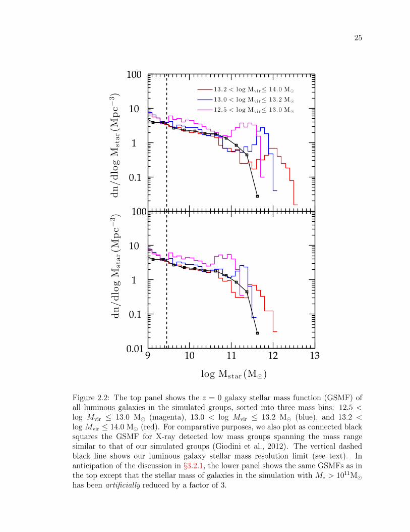
25
0.1
1
10
100
dn/dlogM
star(M
pc−
3 )
9 10 11 12 130.01
0.1
1
10
100
log Mstar (M⊙)
dn/dlogM
star(M
pc−
3 )
13.2 < log Mvi r≤ 14.0 M⊙
13.0 < log Mvi r≤ 13.2 M⊙
12.5 < log Mvi r≤ 13.0 M⊙
Figure 2.2: The top panel shows the z = 0 galaxy stellar mass function (GSMF) ofall luminous galaxies in the simulated groups, sorted into three mass bins: 12.5 <log Mvir ≤ 13.0 M (magenta), 13.0 < log Mvir ≤ 13.2 M (blue), and 13.2 <log Mvir ≤ 14.0 M (red). For comparative purposes, we also plot as connected blacksquares the GSMF for X-ray detected low mass groups spanning the mass rangesimilar to that of our simulated groups (Giodini et al., 2012). The vertical dashedblack line shows our luminous galaxy stellar mass resolution limit (see text). Inanticipation of the discussion in §3.2.1, the lower panel shows the same GSMFs as inthe top except that the stellar mass of galaxies in the simulation with M∗ > 1011Mhas been artificially reduced by a factor of 3.

26
ρm,vir(z) = ∆vir(z) · E2(z)ρcrit(0), (2.3)
where E(z) ≡ H(z)/H0 is the dimensionless Hubble parameter given by
E2(z) = 1− Ωm,0 + (1 + z)3Ωm,0,
and the virial overdensity factor is well-described by the following fitting function
(c.f ., Babul et al., 2002):
∆vir(z) = 49 + 96Ωm(z) +200Ωm(z)
1 + 5Ωm(z),
Ωm(z) =Ωm,0(1 + z)3
1− Ωm,0 + Ωm,0(1 + z)3.
We will refer to the radius of this sphere as the virial radius, Rvir, and the mass
enclosed as the virial mass of the halo, Mvir. Occasionally, we will reference M∆
instead of Mvir. M∆ is the enclosed mass inside a sphere centered on the halo center
within which the mean mass density is ∆ ·ρcrit(z) = ∆ ·E2(z)ρcrit(0). Commonly used
values of ∆ are 200, 500 and 2500. The mapping between these different quantities
is redshift-dependent. At z = 0,
Mvir ≈ 1.2M200 and M500 ≈ 0.7M200,
Rvir ≈ 1.36R200, R500 ≈ 0.67R200, and R2500 ≈ 0.27R200.
In Figure 2.1, we show the z = 0 mass functions of all halos in the simulation
volume (black curve), as well as halos with at least three (red), two (blue) and one
(magenta) “luminous” galaxies (defined below). We identify groups (and clusters) of
galaxies as halos containing ≥ 3 “luminous” galaxies. On mass scales ≥ 1013 M,
nearly all halos have at least 3 galaxies while in the mass range 1012 M <∼Mvir <∼1013 M, only a fraction of the halos do. There are a total of 902 groups in our
simulation volume at z = 0.
Galaxies in the simulation volume are identified using the group-finding algorithm
Spline Kernel Interpolative Denmax (SKID)1 to locate gravitationally bound clumps
of star particles and cold (T < 3× 10⁴ K) gas particles that are eligible to form stars
(c.f ., Oppenheimer et al., 2010). We identify a galaxy as “resolved” if the total mass
in cold gas and stars is ≥ 2.9×10⁹ M and “luminous” if its stellar mass is ≥ 2.9×10⁹
1http://www-hpcc.astro.washington.edu/tools/skid.html
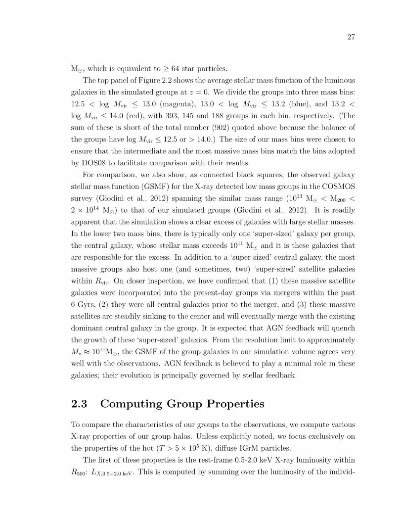
27
M, which is equivalent to ≥ 64 star particles.
The top panel of Figure 2.2 shows the average stellar mass function of the luminous
galaxies in the simulated groups at z = 0. We divide the groups into three mass bins:
12.5 < log Mvir ≤ 13.0 (magenta), 13.0 < log Mvir ≤ 13.2 (blue), and 13.2 <
log Mvir ≤ 14.0 (red), with 393, 145 and 188 groups in each bin, respectively. (The
sum of these is short of the total number (902) quoted above because the balance of
the groups have log Mvir ≤ 12.5 or > 14.0.) The size of our mass bins were chosen to
ensure that the intermediate and the most massive mass bins match the bins adopted
by DOS08 to facilitate comparison with their results.
For comparison, we also show, as connected black squares, the observed galaxy
stellar mass function (GSMF) for the X-ray detected low mass groups in the COSMOS
survey (Giodini et al., 2012) spanning the similar mass range (1013 M < M200 <
2 × 10¹⁴ M) to that of our simulated groups (Giodini et al., 2012). It is readily
apparent that the simulation shows a clear excess of galaxies with large stellar masses.
In the lower two mass bins, there is typically only one ‘super-sized’ galaxy per group,
the central galaxy, whose stellar mass exceeds 1011 M and it is these galaxies that
are responsible for the excess. In addition to a ‘super-sized’ central galaxy, the most
massive groups also host one (and sometimes, two) ‘super-sized’ satellite galaxies
within Rvir. On closer inspection, we have confirmed that (1) these massive satellite
galaxies were incorporated into the present-day groups via mergers within the past
6 Gyrs, (2) they were all central galaxies prior to the merger, and (3) these massive
satellites are steadily sinking to the center and will eventually merge with the existing
dominant central galaxy in the group. It is expected that AGN feedback will quench
the growth of these ‘super-sized’ galaxies. From the resolution limit to approximately
M∗ ≈ 1011M, the GSMF of the group galaxies in our simulation volume agrees very
well with the observations. AGN feedback is believed to play a minimal role in these
galaxies; their evolution is principally governed by stellar feedback.
2.3 Computing Group Properties
To compare the characteristics of our groups to the observations, we compute various
X-ray properties of our group halos. Unless explicitly noted, we focus exclusively on
the properties of the hot (T > 5× 10⁵ K), diffuse IGrM particles.
The first of these properties is the rest-frame 0.5-2.0 keV X-ray luminosity within
R500: LX,0.5−2.0 keV. This is computed by summing over the luminosity of the individ-

28
ual IGrM gas particle within a distance r ≤ R500 of the halo center. The emission
characteristics of gas particles is computed using the Astrophysical Plasma Emission
Code2 (APEC) from Smith et al. (2001) assuming that the gas is optically thin and
in collisional ionization equilibrium. APEC uses the particles mass, SPH-weighted
density, temperature and the metallicity as input, and outputs X-ray spectra, from
which the luminosity is computed by summing the intensities over the required range
of photon energies (e.g. 0.5-2.0 keV). Contributions to line and continuum emission
associated with each of the individually tracked elements (iron, oxygen, silicon and
carbon, along with hydrogen and helium) are computed separately and summed. The
abundances of all the other elements are specified assuming that their abundance ra-
tios relative to iron is solar (Anders & Grevesse, 1989). We note, however, that our
results are not sensitive to the latter because in the IGrM temperature and density
regime, the line emission is dominated by iron, oxygen and silicon.
To study the metal content of the IGrM, we consider two complementary measures:
the mass-weighted and emission-weighted abundances, defined respectively as
Zmwq =
ΣiZq,imi
ΣNi mi
and Zewq =
ΣiZq,iLi
ΣNi Li
, (2.4)
In these equations, “q” is the metal species under consideration, Zq,i is the SPH
kernel-weighted abundance of the ith particle, mi is its mass, and Li is the X-ray
luminosity of that particle. The sums run over all IGrM particles within the volume
under consideration. Additionally, to facilitate comparison between numerical and
observational results, we scale and report all metal abundance estimates in terms of
the solar “photosphere abundance” values from Anders & Grevesse (1989): that is,
ZO, = 0.009618, ZSi, = 0.0007109 and ZFe, = 0.001875.
We also compute two different temperature measures of the hot gas in our groups.
Observationally, the temperature of the hot gas is determined by fitting its observed
X-ray spectrum. Generally, the spectrum within a beam is a composite of the con-
tinuum and the line radiation from a range of gas phases with varying temperatures
and metallicity. Since the emission from individual components cannot be spectrally
distinguished as of yet, and the statistical quality of the observations is insufficient to
detect all the features in the spectrum, and since the spectrum itself is only available
within a limited range of frequencies, the current convention is to compare the com-
posite spectrum with single-temperature, single-metallicity thermal plasma models,
2http://cxc.harvard.edu/atomdb/sources apec.html
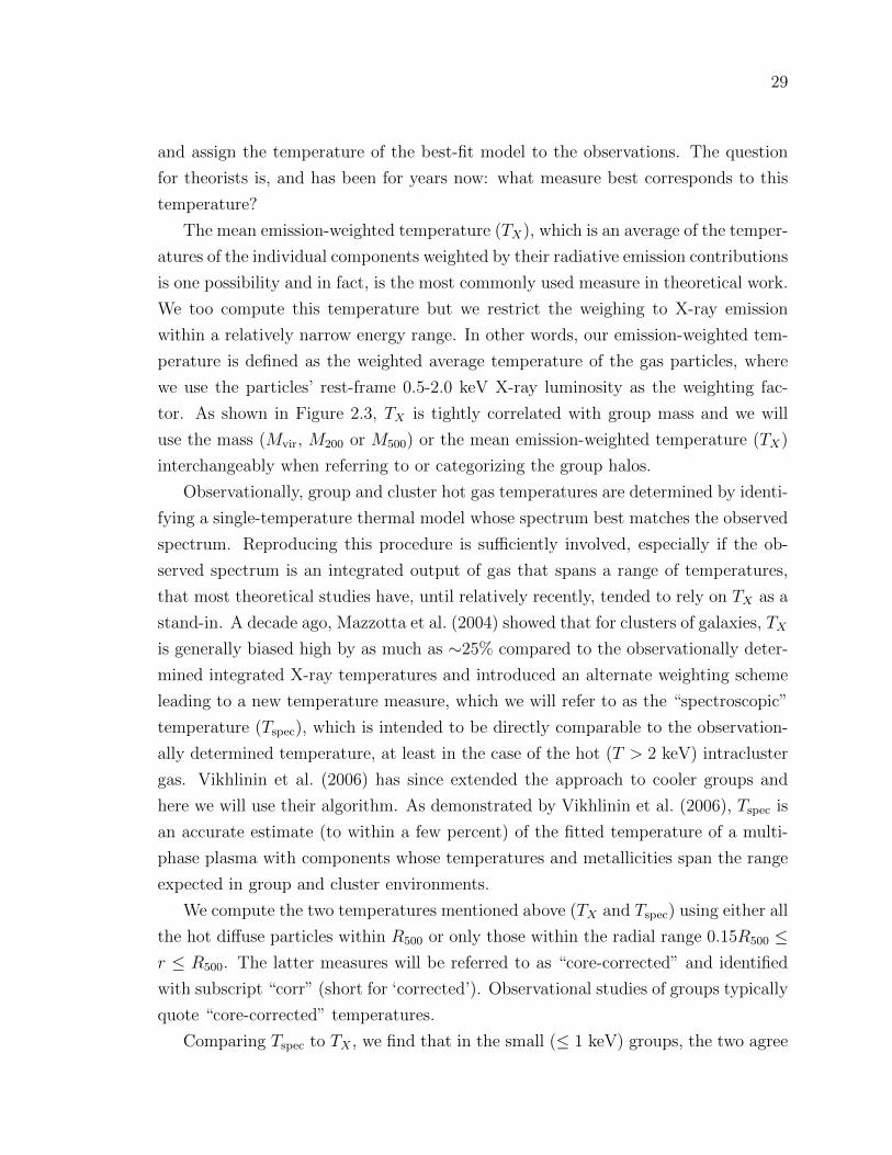
29
and assign the temperature of the best-fit model to the observations. The question
for theorists is, and has been for years now: what measure best corresponds to this
temperature?
The mean emission-weighted temperature (TX), which is an average of the temper-
atures of the individual components weighted by their radiative emission contributions
is one possibility and in fact, is the most commonly used measure in theoretical work.
We too compute this temperature but we restrict the weighing to X-ray emission
within a relatively narrow energy range. In other words, our emission-weighted tem-
perature is defined as the weighted average temperature of the gas particles, where
we use the particles’ rest-frame 0.5-2.0 keV X-ray luminosity as the weighting fac-
tor. As shown in Figure 2.3, TX is tightly correlated with group mass and we will
use the mass (Mvir, M200 or M500) or the mean emission-weighted temperature (TX)
interchangeably when referring to or categorizing the group halos.
Observationally, group and cluster hot gas temperatures are determined by identi-
fying a single-temperature thermal model whose spectrum best matches the observed
spectrum. Reproducing this procedure is sufficiently involved, especially if the ob-
served spectrum is an integrated output of gas that spans a range of temperatures,
that most theoretical studies have, until relatively recently, tended to rely on TX as a
stand-in. A decade ago, Mazzotta et al. (2004) showed that for clusters of galaxies, TX
is generally biased high by as much as ∼25% compared to the observationally deter-
mined integrated X-ray temperatures and introduced an alternate weighting scheme
leading to a new temperature measure, which we will refer to as the “spectroscopic”
temperature (Tspec), which is intended to be directly comparable to the observation-
ally determined temperature, at least in the case of the hot (T > 2 keV) intracluster
gas. Vikhlinin et al. (2006) has since extended the approach to cooler groups and
here we will use their algorithm. As demonstrated by Vikhlinin et al. (2006), Tspec is
an accurate estimate (to within a few percent) of the fitted temperature of a multi-
phase plasma with components whose temperatures and metallicities span the range
expected in group and cluster environments.
We compute the two temperatures mentioned above (TX and Tspec) using either all
the hot diffuse particles within R500 or only those within the radial range 0.15R500 ≤r ≤ R500. The latter measures will be referred to as “core-corrected” and identified
with subscript “corr” (short for ‘corrected’). Observational studies of groups typically
quote “core-corrected” temperatures.
Comparing Tspec to TX , we find that in the small (≤ 1 keV) groups, the two agree

30
−1 −0.5 0 0.511
12
13
14
15
log Tx (keV)
logM
vir(M
⊙)
N ≥ 3
N ≥ 2
Figure 2.3: Mvir−TX relation of galaxy groups with at least three (red) and two (blue)luminous galaxies. TX is tightly correlated with Mvir and follows the scaling relation:Mvir ∝ T 1.7
X . Groups that lie significantly off this relationship are located near largersystems and are “contaminated” by the latters’ hot diffuse gas. Excluding groupswith fewer than three luminous galaxies, eliminates most of these “contaminated”halos.

31
with each other to within ∼3%, in agreement with results shown in Vikhlinin et al.
(2006). However, in hotter systems the divergence is significant enough to be a cause
for concern. We discuss this further in the next section. We also note that neither
Tspec nor TX is an unbiased measure of the actual mean temperature of the gas, which
is much better approximated via a mass-weighted average.
Finally, we point out that to compare the X-ray scaling relations for our simulated
groups across different redshifts, we adopt the common convention in the literature
and plot quantities motivated by the self-similar model of group and cluster halos
(Kaiser, 1986). In this model, the scaling relations are preserved when using the
quantities LX(z)E(z)−1, M∆(z)E(z) and S∆(z)E(z)4/3, where E(z) ≡ H(z)/H0 is
the dimensionless Hubble parameter (c.f., equation 2.3), instead of LX(z), M∆(z) and
S∆(z). The self-similar model assumes that the profiles describing the internal struc-
ture of all groups and clusters have the same functional form, with the gas properties
created through gravitational collapse alone, so that these properties scale only with
the system mass and the critical density at the time of observation. Strictly speaking,
the self-similar model is an anachronism in that it does not account for processes like
radiative cooling or heating of the gas by stellar (or AGN) winds and jets, or for
a variation in the IGrM fraction with halo mass. As a result, the observed scaling
with mass deviates from the predictions of this model. Nonetheless, the observed
scaling with redshift (for moderate redshift values) agrees surprisingly well with the
self-similar predictions, suggesting that over limited periods of time the systems may
well be evolving in a self-similar fashion. For further details, we refer the readers to
§3.9 of Kunz et al. (2012) and to Ettori (2015).
32
Chapter 3
THE SIMULATED PROPERTIES
OF THE IGRM
This chapter is organized as follows: In Section 3.1, we discuss the global X-ray
properties of our galaxy groups, focusing on three most commonly discussed group
X-ray scaling relations: the (X-ray) luminosity-temperature, the luminosity-mass, the
mass-temperature and the entropy-temperature relations. We explore the evolution
of the model scaling relations over the redshift range 0 ≤ z ≤ 3 and also compare
the z = 0 relations to the observational results. We discuss the baryonic content of
the simulated groups in Section 3.2, investigating the variation in the total baryon
fraction as well as the stellar and the hot diffuse IGrM mass fractions with group mass
over the redshift range 0 ≤ z ≤ 3. We compare these fractions with observational
results from both low redshift groups as well as more recent results from groups at
redshifts out to z ∼ 1, and we provide a detailed analysis of the assembly of groups
total mass, IGrM, and stellar mass. We then investigate the enrichment of the IGrM
in Section 3.3, looking at the sources of the iron, silicon and oxygen, the abundance
ratios, etc. Finally, we summarize and discuss our findings in Section 3.4.
3.1 GLOBAL X-RAY PROPERTIES OF GALAXY
GROUPS
In this section, we discuss some of the global properties of galaxy groups, focusing
on the observed X-ray scaling relations, of the simulated z = 0 groups and compare
these to those of simulated groups at earlier epochs (z = 0.5 to 3.0), and to available

33
observations. As we shall show, even in the absence of AGN feedback, the present
model does remarkably well in accounting for the observations.
3.1.1 The Mass-Luminosity-Temperature Scaling Relations
In the absence of feedback and cooling flows, the X-ray luminosity on the group scale
ought to scale with the mean gas temperature of the IGrM as LX ∝ T (Balogh,
Babul & Patton, 1999; Babul et al., 2002). This relationship is flatter than the
more familiar LX ∝ T 2 scaling in situations where bremsstrahlung dominates the
X-ray emission because at temperatures less than 1 keV recombination radiation is as
important, if not more, than bremsstrahlung. The observed scaling relationship for
groups, LX ∝ T 4, however, is much steeper (Helsdon & Ponman, 2000), indicating
that either heating (Balogh, Babul & Patton, 1999; Babul et al., 2002) and/or cooling
(Voit & Bryan, 2001) has significantly altered the hot X-ray gas distribution. Both
processes eliminate the denser, lower entropy, X-ray bright, gas.
Figure 3.1 shows the rest-frame 0.5−2.0 keV X-ray luminosity emitted within the
central R500 versus the mean core-corrected spectroscopic temperature (solid lines)
for the simulated groups at redshifts z = 0 (black), 0.5 (blue), 1 (red), 2 (green)
and 3 (cyan). Once cosmic evolution is taken into account, the group LX − Tspec,corr
curves at z ≤ 1 essentially lie on top of each other. At higher redshifts, however, the
groups – at a given temperature – are less luminous than predicted by the self-similar
evolution model. These trends can be understood in terms of the behaviour of the
hot gas fraction in the groups that we will discuss in the next subsection.
Focusing on the mean LX − Tspec,corr relationship for our simulated z = 0 groups,
we note that this is in good agreement with the observations for Tspec,corr <∼ 1 keV.
In this low temperature regime, the luminosity scales as LX ∝ T 5.5spec,corr. The steep
nature of this relationship is partly due to the use of spectroscopic temperature.
The spectroscopic temperature can differ considerably from the true temperature.
To illustrate this, we plot in Figure 3.1 the LX − T relationship for our z = 0
simulated groups using the core-corrected mass-weighted temperature (Tmw – black
dotted curve). For T<∼1 keV, LX ∝ T 3.8mw. The difference between this relationship and
the self-similar expectation (LX ∝ T ) suggests that the groups have been subjected
to some process that has a greater impact on the IGrM in groups with the shallowest
2 For consistency, we use the same mass-concentration relationship adopted by Lagana, deSouza & Keller (2010).

34
−0.6 −0.4 −0.2 0 0.2 0.4
41
42
43
44
log Tspec,corr (keV)
logLx,0.5−2keV
E(z)−
1(ergs−
1 )
z = 0z = 0.5z = 1z = 2z = 3
mass-weighted temperature
spectroscopic temperature
emission-weighted temperature
Figure 3.1: X-ray luminosity−T relation for simulated groups at z = 0 (black),z = 0.5 (blue), and z = 1 (red), z = 2 (green), and z = 3 (cyan). The solid lines showthe scaling relationship between the X-ray luminosity that is emitted by gas withinR500 and the core-corrected spectroscopic temperature. The error bars indicate 1-σscatter. The dotted and the dashed curves show the mean LX − T for the z = 0simulated groups, where T is the mass-weighted and emission-weighted temperature(both core-corrected), respectively. Squares, stars and triangles show observed lowredshift group data from Osmond & Ponman (2004), Pratt et al. (2009) and Eckmiller,Hudson & Reiprich (2011), respectively. We plot all the groups in Osmond & Ponman(2004) including those with a small radial extent in observable X-rays (i.e. their Hsample). Luminosity in the Pratt et al. (2009) and Eckmiller, Hudson & Reiprich(2011) data is corrected to the 0.5− 2 keV band.

35
12.5 13 13.5 14 14.5
41
42
43
44
logLx,0.1−2.4keV
E(z)−
1(<
R500)(ergs−
1 )
log M500 E(z) (M⊙)
z = 0z = 0.5z = 1z = 2z = 3
Figure 3.2: LX −M relation for simulated groups at z = 0 (black), z = 0.5 (blue),z = 1 (red), z = 2 (green), and z = 3 (cyan). The error bars show 1-σ scatter. Thecircles, stars and squares show data from Eckmiller, Hudson & Reiprich (2011), Prattet al. (2009), and Lagana, de Souza & Keller (2010), respectively. The hydrostaticmass estimates from the first two studies have been corrected for the hydrostaticbias (Haines et al., 2015) and LX,bol from Pratt et al. (2009) have been converted toLX,0.1−2.4 keV. We also convert the weak-lensing M200 values from Lagana, de Souza &Keller (2010) to M500 using an NFW profile,2 and we scale their luminosities using themedian value of LX,0.1−2.4 keV(< R200)/LX,0.1−2.4 keV(< R500) for our simulated groups.The observed groups at z ≤ 0.25, 0.25 < z ≤ 0.75, and z > 0.75 are plotted as black,blue and red symbols, respectively.

36
potential wells (low temperatures) and less so on the gas in groups with the deepest
potential wells (high temperatures). Both heating (or preheating) of the IGrM by the
galactic outflows, which will cause the gas to expand out of (or resist falling into) the
shallowest potential wells, as well as the removal of the IGrM by radiative cooling,
are plausible mechanisms. At this point, we cannot distinguish between these two.
For T > 1.2 keV, the LX − T based on the spectroscopic and the mass-weighted
temperatures converge, implying that in massive groups, the former is a good mea-
sure of the latter. Both scaling relations also start to flatten as bremsstrahlung grows
in importance. However, we note that compared to the observations, the high mass
simulated groups are more luminous, and/or a bit cooler. This suggests that the hot
gas in these systems is denser than in real systems. In the scenario where the galactic
outflows really do impact the gas density in shallow wells, the emergence of overlu-
minous groups as their halo mass approaches (and exceeds) M ≈ 1014 M suggests
that the outflows have become ineffectual and another mechanism is necessary.
For illustrative purposes, we also plot LX − T relationship for the z = 0 groups
using the mean emission-weighted temperature (TX – black dashed curve). Until
relatively recently, this was the relationship used to compare model LX −T to obser-
vations. For the lowest temperature groups, the emission-weighted and the spectro-
scopic temperatures are nearly equal, and the two LX − T curves track each other.
For T > 0.7 keV, the emission-weighted LX − TX deviates from that based on the
spectroscopic temperature and remains in good agreement with the observations.
This agreement, however, is spurious since the observations are based on the spec-
troscopic temperature, and indicates a need for caution: The comparison between
the TX−based relation for simulated groups and the Tspec−based observations masks
the need for an additional heating or redistribution mechanism in the more massive
groups.
It is instructive to compare our results to those of the “stellar feedback only” run
from the OWLS collaboration (referred to as the “Reference Model” in McCarthy
et al. 2010 and as the “ZCool+SF+SN model” in McCarthy et al. 2011). This model
(hereafter referred to as OWLS-stars) primarily accounts for only SNe feedback, which
is implemented via the kinetic wind model of Dalla Vecchia & Schaye (2008), where
the mass loading factor is fixed to constant (η = 2) instead of varying inversely
with galaxy velocity dispersion as in our model and the wind velocity is also set to
a constant, 600 km/s. Comparing the resultant LX − TX for the simulated groups
(c.f., right panel of Figure 6 in McCarthy et al., 2010), we find that the groups in

37
the OWLS-stars run are about a factor of ∼ 10 more luminous than our groups at
T ≈ 0.5 keV, and about a factor of ∼ 2 more luminous than our groups at T ≈ 1 keV.
While our results match the observed LX − TX relationship, theirs lie systematically
above the observations and define a shallower trend. A comparison with the results
shown in McCarthy et al. (2011) indicates that this difference is due to a larger IGrM
component within R500 in the OWLS-stars groups and possibly that the IGrM is
more centrally concentrated and hence, denser. We will comment on this further in
the next section where we discuss the IGrM and the baryon fractions in our groups.
Finally, we note that the error bars on the simulation results indicate 1-σ scatter
above and below the mean. The scatter in the observational data is significantly
larger. There are a number of possible reasons for this difference. First, our simula-
tions are missing AGN feedback and one can imagine that the variations introduced
by yet another heating/redistribution mechanism could increase the dispersion in the
X-ray luminosity of the simulated groups at a fixed temperature (see, for example,
McCarthy et al., 2010). The observations, however, are also not homogeneous. For
instance, we plot all groups in Osmond & Ponman (2004), including those in which
the X-ray emission is only detected to a relatively small radial extent. This can arti-
ficially enhance the scatter. In fact, most group samples, including the ones plotted,
are not statistically representative (O’Sullivan et al., 2014) and the inhomogeneities
and biases will also be reflected in the scatter.
Figure 3.2 shows the LX −M trends for the simulated groups at redshifts z = 0
(black), z = 0.5 (blue), z = 1 (red), z = 2 (green) and z = 3 (cyan). This time
we plot the rest-frame 0.1-2.4 keV X-ray luminosity to facilitate comparison with
available observations. Like the LX − Tspec,corr curves, once cosmic evolution is taken
into account through the dimensionless Hubble parameter E(z), the LX −M curves
for the z ≤ 1 group populations scale as Lx ∝M1.7500 and essentially lie on top of each
other, implying a self-similar evolution over this redshift range. Like the LX−Tspec,corr
relations, the higher redshift curves lie off those at z ≤ 1 and the deviation goes in the
same direction. The groups at a given value of ME(z) – note that temperature and
ME(z) are equivalent measures of the depth of the gravitational potential well – are
less luminous than predicted by the self-similar evolution model and the underlying
reasons, on which we will elaborate when we discuss the behaviour of the hot gas
fraction in the groups, are also the same.
There are two different types of observational data shown in the plot: One set
(black circles and stars), where the group masses are in fact hydrostatic mass estimates

38
derived from the X-ray measurements by Eckmiller, Hudson & Reiprich (2011) and
Pratt et al. (2009), respectively, and another (black, blue and red squares), where the
masses are derived using weak lensing methods (Lagana, de Souza & Keller, 2010). It
is well known that the hydrostatic masses typically underestimate the true mass and
to facilitate a fair comparison with our actual mass determinations, we have corrected
the Pratt et al. (2009) and Eckmiller, Hudson & Reiprich (2011) masses using the
bias factor determined by Haines et al. (2015) (see also Mahdavi et al., 2013). Our
numerical results are in good agreement with the observational results. Moreover,
the fact that the LX−M trends delineated by the black, blue and red points show no
significant offsets from each other suggests that the evolution of the observed group
LX −M relation is consistent with that predicted by the self-similar model over the
redshift range 0 ≤ z < 1, which is also in agreement with our numerical results.
Figure 3.3 shows the M − Tspec,corr trends for the simulated groups at redshifts
z = 0 (black), z = 0.5 (blue), z = 1 (red), z = 2 (green) and z = 3 (cyan).
Once cosmic evolution is taken into account, all the curves, even those for z > 1
groups, lie on top of each other. The shape of these curves differs from that shown in
Figure 2.3 because there we had plotted mass versus emission-weighted temperature
whereas here we are using the core-corrected spectroscopic temperature. Comparing
the M − T relation for our simulated z = 0 groups to that of OWLS-stars groups
(c.f., Figure 5 of McCarthy et al., 2010, – this figure shows mass versus emission-
weighted temperature whereas we plot mass versus spectroscopic temperature), we
find that the two are in excellent agreement with each other once the differences
between the two temperatures at Tspec,corr >∼ 0.8 keV are accounted for.
As in Figure 3.2, we plot corrected hydrostatic masses (squares and triangles) and
masses derived from weak lensing analyses (black and blue diamonds). Within the
scatter, all the data (weak lensing and X-ray based, present-day and at moderate
redshift) are consistent with each other. Focusing on measurements with Tspec,corr >
0.8 keV, the scaling of mass with temperature can be well described by M500 ∝T 1.6
spec,corr, which is consistent with the self-similar scaling relationship. The numerical
trends, on the other hand, are steeper in the neighbourhood of 1 keV but flattens
at both higher and lower temperatures. In spite of this, the numerical results are
consistent with the observations except perhaps for the most massive groups with
M500>∼ 1014 M. In these massive systems, the temperature in the simulated systems
seems to be a bit cooler than that in the observed systems. We note that this
divergence at the high mass end is also present in the LX − Tspec,corr plot.

39
−0.6 −0.4 −0.2 0 0.2 0.4
12.5
13
13.5
14
14.5
log[M
500E(z)]
(M⊙)
log Tspec,corr (keV)
z = 0z = 0.5z = 1z = 2z = 3
Figure 3.3: M − Tspec,corr relation for simulated groups at z = 0 (black), z = 0.5(blue), z = 1 (red), z = 2 (green), and z = 3 (cyan). The error bars show 1-σscatter. The black squares and triangles show the results from Sun et al. (2009)and Eckmiller, Hudson & Reiprich (2011). The hydrostatic mass estimates given inthese two studies have been corrected for the hydrostatic bias (Haines et al., 2015).We also note that the temperatures in the latter study are not always extractedin a consistent, systematic fashion. The diamonds show results from Kettula et al.(2013); their masses are weak-lensing estimates. The observed groups at z ≤ 0.25and 0.25 < z ≤ 0.75 are plotted as black and blue symbols, respectively.

40
At various points in the preceding discussion, we have noted that the trends
exhibited by the simulated groups in the LX−Tspec,corr−M space are the consequences
of two different types of processes: (1) the structure of the intergalactic medium that
collapses to form the IGrM and, therefore, the properties of the IGrM itself, are
altered by the galactic outflows from an earlier (z > 2) generation of galaxies; and
(2) heating and/or cooling processes occurring once the groups form can convert the
cooler, denser, X-ray luminous gas into either hotter, more diffuse (and therefore, less
luminous) gas, or into cold, dense gas that is effectively dark in the X-rays. To gain
insights into the relative importance of these effects, we examine the entropy of the
hot X-ray emitting gas.
3.1.2 The Entropy-Temperature Scaling
Entropy is a very useful physical quantity to consider when the IGrM is subject to
cooling and heating processes because the former typically lowers the entropy while
the latter always raises it. This is not the case with either density or temperature
because heating can cause the gas to expand, potentially lowering both quantities
(see McCarthy et al., 2008, for a more detailed discussion). Additionally, the gas
distribution will tend to organize itself so that the lowest entropy gas is at the group
centre and the highest is at the group periphery. On the other hand, in the present
situation, there is an additional complication to keep in mind: If cooling is able to
cause the low entropy IGrM in the center to drop out and settle in the central galaxy,
higher entropy gas from further out will flow in to take its place and the entropy
in the centre will appear “enhanced” unless cooling is able to erode the entropy of
this inflowing gas as quickly as it flows in. This effect was first seen in the numerical
simulation by Lewis et al. (2000) and discussed more fully by Voit & Bryan (2001).
In Figure 3.4, we show the cosmic expansion corrected gas entropy at R500 (top
panel) and R2500 (bottom panel), in present-day groups (black solid curve) as well
as for groups at z = 0.5 (blue), z = 1 (red), z = 2 (green), and z = 3 (cyan),
as a function of the integrated core-corrected spectroscopic temperature of the IGrM
within R500 . We also plot entropy estimates from the X-ray observations of Sun et al.
(2009), computed using the deprojected temperature and electron density profiles. To
be precise, we are not plotting the actual thermodynamic specific entropy, but rather
its widely accepted proxy2 given by
2The ‘entropy proxy’ (S) and the thermodynamic specific entropy (s) are related to each other

41
−0.6 −0.4 −0.2 0 0.2 0.4
1.5
2
2.5
log Tspec,corr (keV)
logS2500E
4/3 (z)(k
eVcm
2)
z = 0z = 0.5z = 1z = 2z = 3
1.5
2
2.5
3
logS500E
4/3 (z)(k
eVcm
2)
S500
S2500
Figure 3.4: Gas entropy at R500 (top panel) and R2500 (bottom panel) of the simulatedgroups at z = 0 (black), z = 0.5 (blue), z = 1 (red), z = 2 (green) and z = 3 (cyan),as a function of core-corrected spectroscopic temperature. The error bars show 1-σscatter. The observational data of the low redshift sample from Sun et al. (2009,hereafter S09) is shown by black squares. The dashed lines in the top and bottompanels represent the power-law fits to the S − T relation at the two different radiifor the full group+cluster sample from S09, with a power law index of 1 and 0.74,respectively.

42
S(r) =kBTspec(r)
ne(r)2/3, (3.1)
where kB is the Boltzmann constant, and Tspec(r) and ne(r) are, respectively, the
spectroscopic temperature and the electron number density within a thin spherical
shell at radius r. We shall, hereafter, refer to S(r) as ‘entropy’.
Focusing first on the R500, we see that scaled entropy systematically declines with
time. The change is much greater at high redshifts (z > 1) than at low redshifts
(z < 1) and also, much more stronger in groups with shallow potential wells than in
those with deep potential wells. Both results are primarily driven by the evolution
in the IGrM density at R500. For group halos of a given temperature, if we take the
present-day value of IGrM density at R500 as a reference, then we are led to conclude
that the IGrM density at R500 at an earlier epoch is not E(z)2 times the present-day
value, as would be expected if the IGrM density were evolving self-similarly. Rather,
it is lower than the expected value and hence, the cosmic expansion corrected entropy
is higher. Put another way, the halos at z = 3 are IGrM poor (relative to the total
matter). As the halos grow, they encompass additional dark and baryonic matter
but the ratio of baryons-to-dark matter is larger than the universal value. In effect,
the groups are recapturing some of the baryons that were ejected from their member
galaxies at earlier times, in addition to the usual complement associated with the
accreting dark matter (reminiscent of the “outside-in” IGM enrichment scenario of
Oppenheimer et al. 2012). The higher temperature groups are able to recapture a
greater fraction of the previously expelled baryons at an earlier time (z > 2) than
the lower temperature groups. The outcome of this differential accretion of baryons
and dark matter is that the density of hot gas in the groups evolves differently from
self-similar expectations – i.e., until z ≈ 1, after which the evolution of the entropy
and the density for all the group halos is consistent with self-similar evolution. We
will examine the density and entropy profiles in detail in future work. However, this
general behaviour also explains the self-similar evolution of the LX − Tspec,corr and
LX −M from z = 0 to z = 1 and then, the decrease in the amplitude of the (cosmic
expansion corrected) scaling relation from z = 1 to z = 3 (c.f., Figures 3.1 and 3.2).
At higher redshifts, the groups of a given temperature or ME(z) (both are equivalent
measures) are not as luminous as they ought to be if they were evolving self-similarly
because the IGrM is not as dense as self-similarity would predict.
as ds ∝ d lnS (see Balogh, Babul & Patton, 1999).

43
In contrast with S500, S2500 evolves somewhat differently. The scaled entropy
evolves self-similarly from z ≈ 2 to the present and even between z = 3 and z = 2,
the change is relatively mild. The core regions tend to form earlier and we expect that
they will settle down into a steady-state configuration at an earlier epoch. DOS08
compared the core entropies of groups in a simulation with and without outflows
and found that the gas in the former case had higher entropy. This is a non-trivial
result. As we mentioned above, it is not unexpected to see elevated entropies at
R2500 in simulations with cooling, star formation and inefficient stellar feedback (here-
after simulations – for more details about such simulations, see Lewis et al., 2000;
Kravtsov, Nagai & Vikhlinin, 2005, and DOS08), relative to a non-radiative simula-
tion (c.f., Figure 10 of Lewis et al. 2000). The inclusion of outflows, however, could
just as easily have led to still higher core entropies, or lower core entropies. As DOS08
explain, the latter can occur if heating from the outflows just balances cooling, and
the low-entropy gas remains in place unchanged, i.e., it is neither removed via cooling
nor raised to a higher adiabat. The outflows in our simulations, on average, heat the
IGrM at least close to the centre of the groups.
Comparing S500 and S2500 entropy results for our simulated groups to the obser-
vations, we find that the IGrM entropy at R500 in our massive groups is consistent
with the observations. Sun et al. (2009) find that the observed S500 values scale
with the integrated core-corrected spectroscopic temperature of the gas within R500
as S500 ∝ Tspec,corr (dashed line) across their full sample of groups and clusters. Our
simulation results also follow the same scaling for Tspec,corr > 0.3 keV. Below this
threshold, S500 in the simulated groups flattens. This flattening is because of a de-
crease in the IGrM density with decreasing group mass. We will discuss this further in
the next subsection. At R2500, Sun et al. (2009) find that the observed entropy scales
as S2500 ∝ T 0.74spec,corr (dashed line). The S2500 of the groups in the simulated sample
is less steep, scaling with temperature as S2500 ∝ T 0.50spec,corr, and the simulated groups
at the high mass end have approximately 40% lower core entropies compared to the
observations. One explanation is that the density of IGrM in the cores of the massive
simulated groups is slightly higher than in real groups and this, in turn, would explain
why massive simulated groups seem to be somewhat more X-ray luminous than their
real counterparts.
Comparing our entropy results to those of groups in the OWLS-stars run (see
Figure 2 in McCarthy et al., 2010), we find that entropy at R500 in the two simulations
is very similar. At R2500, however, the entropy in the OWLS groups is lower than

44
in our groups by approximately 25 − 30%. This supports our previous conjecture
that the IGrM in OWLS groups is more centrally concentrated than in our groups,
which in turn would explain the differences in the X-ray luminosities of the two group
populations.
Overall our stellar-powered wind model fares remarkably well when it comes to
matching the observed group LX − Tspec,corr − M scaling relations except perhaps
in the most massive groups. The behaviour of the IGrM entropy at R2500 and R500
suggests that the principal variable governing the behaviour of these relationships in
our simulated groups is the IGrM density.
3.2 THE BARYON CONTENT OF GALAXY GROUPS
We now turn to direct determinations of the total baryon fraction as well as the
stellar and the IGrM gas mass fractions in the simulated groups to confirm whether
the IGrM density behaves as we have argued above, and try to understand the reasons
behind its behaviour. The partitioning of the baryons between stars and hot gas is
interesting in and of itself. We know that our model is not able to suppress the
overproduction of stars in the largest galaxies in the groups (c.f., Figure 2.2) but
by looking into the issue more carefully, we hope to understand when and where the
model starts to fail. Additionally, we also quantify the assembly of the groups using
several different measures.
3.2.1 Stellar, Gas and Total Baryon Fractions
The sequence of plots in the left panel of Figure 3.5 shows the total baryon, T >
5× 10⁵ K, hot, diffuse gas (IGrM), stellar, and cold gas fractions in simulated groups
at z = 0, as function of the total group mass. All the quantities are computed with
R500 to facilitate comparisons with the observations. The plots in the right column
show the same mass fractions within R200 to illustrate their behaviour across group
populations at different redshifts as well as beyond just the inner regions of the halos.
The coloured lines show the results for groups at z = 0 (black), 0.5 (blue), 1.0 (red),
1.5 (magenta), 2.0 (green) and 3.0 (cyan). On the x-axis, we plot M200E(z) so that
we can compare populations of halos with potentials of similar depths across the
different epochs. Baryon properties, as well as the impact of feedback and radiative
cooling, both tend to be strongly correlated with the depth of the halos’ gravitational

45
0.04
0.08
0.12
0.16
0.2M
bar/M
500
0
0.04
0.08
0.12
MIG
rM/M
500
12.5 13 13.5 14 14.50
0.04
0.08
0.12
Mcold/M
500
log M500 (M⊙)
0
0.04
0.08
0.12
M∗/M
500
0.04
0.08
0.12
0.16
0.2
Mbar/M
200
0
0.04
0.08
0.12
MIG
rM/M
200
12.5 13 13.5 14 14.50
0.04
0.08
0.12
Mcold/M
200
log M200 E(z)(M⊙)
0
0.04
0.08
0.12
M∗/M
200
z = 0z = 0.5z = 1z = 1.5z = 2z = 3
Figure 3.5: Left column: Stellar and gas mass fractions within R500 in simulated z = 0groups. Top panel: Total baryonic fraction. The black line indicates the cosmologicalvalue, Ωb/Ωm = 0.176. The symbols (see text for details) show observational estimatesfor hot gas + stars. Error bars depict 1-σ scatter. Second panel: Hot gas fraction.Third panel: Stellar mass fraction. The simulation results include stars in the galaxiesas well as those comprising the diffuse intragroup stars [IGS]) component. Of theobservational estimates, only the golden circles (Gonzalez et al., 2013) account forthe IGS. Bottom panel: Cold gas fraction (i.e. diffuse gas with T < 5×10⁵ K and thegalactic ISM). Right column: The same mass fractions for simulated groups at z = 0(black), z = 0.5 (blue), z = 1 (red), z = 1.5 (magenta), z = 2 (green) and z = 3 (cyan)computed within R200 to facilitate comparison with observations. Triangles, circlesand squares are observational results from McCourt, Quataert & Parrish (2013), vander Burg et al. (2014) and Connelly et al. (2012), respectively. Data for z <∼ 0.25groups are in black, 0.25 < z<∼ 0.75 in red, and 0.75 < z<∼ 1.25 groups in blue. Thesedo not account for the IGS.

46
potential well. For completeness, we note that we have tracked the evolution of
individual groups in the right column of Figure 3.5 and find that once formed, they
do not simply evolve vertically in these plots. Rather, they move both vertically up
or down (depending on the quantity under consideration) with decreasing redshift,
transitioning from one coloured line to the next, while also generally sliding to the
right along the x-axis. This is because the masses of individual groups generally
grow faster than expected under the self-similar growth model; i.e., they increase
faster than M200(zgroup) [E(zgroup)/E(z)], where zgroup is the redshift at which the
most massive progenitor halos of the present-day groups first acquire three luminous
galaxies and as per our definition, become ‘groups’. Consequently, the potential well
of individual groups tend to deepen towards the present.
In the first panel of both columns, we investigate the total baryon fraction. The
solid line indicates the cosmological baryon fraction of Ωb/Ωm = 0.176 for the simula-
tion. The red triangles, blue squares, golden circles and orange stars in the left panel
show observational estimates of the fraction of mass in hot gas and stars, which for
massive groups is essentially the same as the total baryon fraction, from Lin, Mohr
& Stanford (2003), Giodini, Pierini & Finoguenov (2009, revised3), Gonzalez et al.
(2013), and Lagana et al. (2013), respectively. Of these, only Gonzalez et al. (2013)
(golden circles) explicitly account for the extended, diffuse intragroup stellar com-
ponent (hereafter referred to as the intragroup stars or IGS). The simulation results
include all stars, those in the galaxies as well as those that belong to the extended
population. In spite of the large scatter in the observed values, the total baryon frac-
tion within R500 in our simulated present-day groups is generally greater than that
in real groups by approximately 35− 40%.
This is the first indication that powerful stellar-powered galactic outflows, in and
of themselves, are not capable of preventing the over-concentration of baryons within
R500 in the simulated groups, in comparison to the observations. This is not to say
that the outflows have no impact on the galaxy groups. The baryon fraction of our
simulated groups is comparable to that seen in non-radiative simulations (see for
instance Crain et al., 2007) – i.e.,simulations that do not allow for cooling. It is most
definitely lower than the values seen in the simulations (Lewis et al., 2000; Kravtsov,
Nagai & Vikhlinin, 2005, DOS08), where the baryon fraction within R500 is typically
3The results for Giodini, Pierini & Finoguenov (2009) shown in Figure 3.5 differ from those in theirpaper because they have been revised as suggested by Leauthaud et al. (2012). See also discussionin Giodini et al. (2012). The stellar masses results presented are derived using the Chabrier IMF.

47
0.1 1 0.5
1
1.5
2
2.5
3
[Mbar(<
R)/M
tot(<
R)]/[Ω
b/Ω
m]
12.5 ≤ log Mvir E(z) < 13
0.1 1 R/R200
13 ≤ log Mvir E(z) < 13.2
0.1 1
13.2 ≤ log Mvir E(z) < 14
z = 0z = 0.5z = 1z = 2z = 3Cool+SF
Figure 3.6: The mean baryon fraction within radius R/R200 in simulated groups atz = 0 groups (black curve), z = 0.5 (blue), z = 1 (red), z = 1.5 (magenta), z = 2(green) and z = 3 (cyan), normalized to the cosmic baryon fraction Ωb/Ωm = 0.176for the simulation. We have sorted the groups into three bins according to the depthof their potential wells: In each panel, the dashed black curve shows the z = 0 meanbaryon fraction profile for the simulation from Lewis et al. (2000), which had nogalactic winds.
48
equal to or even slightly larger than the universal value. Below we try to understand
precisely how the galactic outflows affect the baryon fraction in our simulated groups.
Examining the simulation results more closely, we note that the median value
of the baryon fractions within R500 in the z = 0 groups exhibits a gradual rise
with increasing halo mass, going from ∼ 82% of the universal cosmological value
in the least massive groups to ∼ 90% of the universal value in the most massive
groups. Comparing these results against those for the OWLS-stars groups (in this
case “ZCOOL+SF+SN” simulation; McCarthy et al. 2011), we find good agreement.
The median baryon fractions in the latter groups range from 88% of the cosmological
value in the lower mass groups to 92% in the high mass systems. The median baryon
fractions within R200 of the z = 0 groups also increases gradually with halo mass,
from ∼ 86% of the universal value in our lowest mass groups to ∼ 93% in the high
mass groups. The baryon fractions within R500 are slightly but systematically lower
than within R200 because, in our simulated groups, the principal source of outflows is
the dominant central galaxy and as noted while discussing the IGrM entropy, these
preferentially heat the gas in the central regions.
The trend highlighted above, of lower mass systems being more baryon depleted, is
a common feature of the strong stellar feedback models. In the case of the momentum-
driven wind model, Dave (2009) has shown that the baryon fraction in present-day
Milky Way-sized halos (∼ 1012 M) drops to 60% of the cosmic value and de-
creases further to below 50% of the cosmological value in lower mass galactic halos
(∼ 1010 M). On these galactic scales, the reason is fairly clear. The winds physically
carry away a large fraction of the baryons from such systems and in fact, can drive
down the baryon fraction over regions that extend well beyond the virial radius of
the galactic halos. Similar results are also seen in other “no AGN” simulations where
stellar feedback is implemented via a thermal prescription (see Soko lowska et al.,
2015, and references therein).
As one moves up in halo mass, the deepening gravitational potential wells engender
a transition from a state where the bulk of the baryonic matter within a halo is in
the form of stars and cold gas localized in the galaxy (or galaxies), to one where
the hot diffuse gas component that suffuses the entire halo eventually dominates the
baryon budget. This transition has been discussed in detail by Knobel et al. (2009)
and Gabor & Dave (2015), and references therein. Following Gabor & Dave (2015),
we define the transition point between these two states as one where the hot gas
mass exceeds 50% of the total gas mass. In our simulations, this changeover group

49
mass occurs at M200 ≈ 1.8 × 10¹² M at z = 0, M200 ≈ 3 × 10¹² M at z = 1 and
M200 ≈ 6.3× 10¹² M at z = 2. These masses are comparable to the transition mass
cited in Gabor & Dave (2015) although in detail our transition masses are slightly
larger because we impose an additional constraint that the halos must host at least
three luminous galaxies. The presence of a pervasive IGrM alters the wind dynamics:
Galactic winds flowing through such a medium are subject to hydrodynamic drag,
the relative importance of which grows as the density of the medium increases. In the
case of our group halos, the combination of the deeper gravitational potential wells
and the higher likelihood of strong hydrodynamic interactions results in the winds
being almost completely confined within the halos. So the reduced baryon fraction,
relative to the cosmic mean, is not due to the outflow of the baryons.
Instead, the reduced baryon fraction in the group halos is the result of the following
two effects. First, groups typically form in regions that have been rendered somewhat
baryon deficient by winds from their member galaxies at earlier times. Consequently,
when the groups first form, their baryon fraction can be as low as ∼ 75% of the
cosmic mean, as illustrated by the baryon fraction curve for z = 3 groups in the top
right panel of Figure 3.5. This “baryon depletion” is illustrated much more clearly
in Figure 3.6. At z ≈ 3, for example, the baryon fraction within R200 is 75% − 77%
of the mean value for the simulation, and one would have to go out to ∼ 3R200
before the fraction returns to the cosmic mean. (For comparison, we also show the
baryon fraction profile for a simulation from Lewis et al. (2000); the baryon fraction
never really drops below the mean value and converges to the mean value by R200.)
This depletion is slightly less pronounced in the more massive groups and diminishes
towards the present.
Returning to the top right panel of Figure 3.5, we have noted previously that
individual groups, once formed, tend to grow in mass. And as the halos grow, their
physical reach extends further out. As a result, in addition to the inflow of the usual
baryonic complement of the accreting dark matter, they are also able to recapture an
increasing fraction of the expelled gas previously associated with the group galaxies
(c.f., Ford et al., 2014, for a discussion of a similar phenomenon in galactic halos.),
and the overall baryon fraction increases with halo mass.
This, however, is not all. There is a second effect at play, otherwise we would
expect the baryon fraction to continue rising with decreasing redshift and approach
the mean cosmological value. Instead, we observe a sharp increase in the halo baryon
fraction between z = 3 and z = 2, a much more tempered rise from z = 2 to z = 1,

50
and very little change, if any, thereafter. This second effect is the result of the winds
ejected from the group galaxies interacting with and heating the hot halo gas, which
not only reduces the rate at which the halo gas cools and accumulates in the group
central galaxies but also causes its distribution to remain more extended.
In the preceding discussion, we use the word “extended” deliberately. Hot gaseous
halos generally extend beyond the virial radius (c.f., Bahe et al., 2013; Gabor & Dave,
2015) but in simulations without winds, radiative cooling inside the halos leads to
the loss of pressure support, which then results in a denser, more compact baryon
distribution. In the case of our wind model, the hot halo gas density starts out lower
than usual and it is easier for heating by the winds to compensate for a significant
fraction of the radiative cooling losses and drastically slow down its collapse. As
indicated in the top right panel, halos with gravitational potential wells of a given
depth (i.e.,at a fixed M200E(z)) establish an equilibrium distribution by z = 1, and
the baryon fraction remains essentially constant from z = 1 to the present.
However, the efficacy of the galactic winds to maintain an extended hot gas dis-
tribution via heating drops with deepening potential wells because the characteristic
temperature (Twind) corresponding to the complete thermalization of the kinetic en-
ergy in the outflows from any one galaxy in a group halo, even the dominant galaxy,
does not grow as quickly as the group halo’s virial temperature (Tvir). The reason for
this is that Twind scales as M2/3gal , where Mgal is the mass of individual galaxies, whereas
Tvir grows as M2/3200 and as we explain below, the fraction of the baryons condensing
into the cold gas+stars phase decreases with increasing group halo mass. Moreover,
by virtue of being multi-galaxy systems, even the baryons that have condensed out
are distributed over 3 or more “luminous” galaxies. In the end, the IGrM is not able
to withstand gravitational compression despite being heated.
The second set of panels in Figure 3.5 show the diffuse hot (T > 5 × 10⁵ K)
IGrM gas fraction in the simulated groups. The IGrM fraction within R500 (left
column) nearly doubles, from ∼ 0.05 to 0.1, in going from M500 ≈ 3 × 10¹² M to
M500 ≈ 1014 M. This increase with group mass is the result of the larger mass
systems having deeper potential wells and higher virial temperatures. As a result,
more of the diffuse gas is shock-heated to constitute the IGrM. Additionally, the
deeper potential wells are also better able to compress and confine this gas.
Comparing our results against Figure 4 of McCarthy et al. (2010), we find that
the IGrM gas fraction within R500 of comparable groups at the low mass end of the
group distribution in our simulation is about 30% lower (i.e., 0.053 for our groups

51
versus 0.07 for the OWLS-stars groups) and about 10% lower for the groups at the
high mass end. The lower IGrM fraction is a key reason why our simulated groups
are less X-ray luminous than the OWLS-stars groups. We do note that McCarthy
et al. (2010) define the IGrM using the temperature cut of T > 1× 10⁵ K instead of
T > 5× 10⁵ K, as we have. However, we have recomputed the IGrM fraction for our
groups using this lower threshold and find negligible changes to our results.
Comparing the simulation results for the z = 0 IGrM fraction within R500 (left
panel) against observations (red triangles, open magenta squares, green stars , filled
blue squares, golden circles, and orange stars are data from Lin, Mohr & Stanford
(2003), Sun et al. (2009), Sanderson, O’Sullivan & Ponman (2009), Giodini, Pierini
& Finoguenov (2009), Gonzalez et al. (2013), and Lagana et al. (2013), respectively),
we find that the two are in reasonable agreement. In detail, there is a hint that the
IGrM fraction in the simulated groups is rising slightly faster with increasing group
mass but it is difficult to be more definite given the large scatter in the observations.
Such a trend would, however, be consistent with our previous finding that the most
massive simulated groups are slightly more X-ray luminous than real systems and that
the stellar-powered winds are unable to keep the baryon fraction from creeping up-
wards. Together, all of these suggest the need for another gas heating/redistribution
mechanism.
The right panel in the second row of Figure 3.5 shows the IGrM fraction in the
groups at different redshift. Like the results for the baryon fraction (top right panel),
the IGrM fraction in halos with comparable potential wells increases between z ≈ 3
and z ≈ 1 and then, stabilizes. Since most of the freshly accreted baryons directly
contribute to the IGrM over the epochs and in the halo mass regime being considered,
that the total baryon and the IGrM fractions behave similarly is not surprising.
To investigate the make-up of the present-day IGrM within R200 in detail, we
have tracked all the IGrM gas particles back in time and tagged all those that, at
any point in the past, were bound to a galaxy and enriched while bound. We refer
to this component of the present-day IGrM as “processed” and the rest of the gas as
“unprocessed.”4 We find that the fraction of the present-day IGrM that is “processed”
gas ranges from ∼ 15% in the highest mass groups to 3−4% in the lowest mass groups.
4“Unprocessed” material is essentially gas that has never passed through a galaxy and has en-tered the group halos via diffuse accretion directly from the intergalactic medium. We emphasizethat “unprocessed” should not be interpreted as un-enriched. A significant fraction of the present-day “unprocessed” IGrM has non-primordial metallicity owing to enrichment by the diffuse IGScomponent.

52
(We relaxed the “enriched while bound” condition and repeated the analysis, and got
identical results.) This increase in the fraction of “processed” IGrM or equivalently,
the decrease in the fraction of “unprocessed” IGrM, with increasing halo mass is
the continuation of the trend observed by Ford et al. (2014). On galactic scales
(M200 ∼ 1011 M), Ford et al. (2014) find that the “unprocessed” component, which
they call “ambient gas”, makes up nearly all of the hot gas. That the fraction of
processed gas in the IGrM is relatively small even in the most massive groups may
seem surprising but only a small fraction of the metal-rich wind material ejected from
central galaxies, for example, thermalizes at T > 5×10⁵ K and remains in the IGrM.
Acting more like a galactic fountain, the most of the wind lifts off from the galaxy,
transfers its kinetic energy to the ambient gas, and falls back into the galaxy. This
behaviour has been discussed in detail in Oppenheimer et al. (2010) and Ford et al.
(2014)
The fraction of the gas that is heated to T > 5 × 10⁵ K and is lost to cooling is
relatively small. Over a Hubble time, it ranges from ∼10% at M200 = 3 × 10¹² M,
to ∼2.5% at M200 = 3× 10¹³ M, to ∼0.2% at M200 = 3× 10¹⁴ M. Most of the gas
that drops out of the IGrM is initially heated only to 5 × 10⁵ K < T < 3 × 10⁶ K.
Metal-enriched IGrM in this temperature range sits on the broad peak of the cooling
curve and is subject to efficient cooling, which even heating by stellar-powered galactic
winds/fountains cannot fully offset.
The third set of panels in Figure 3.5 show the stellar mass fraction in our simulated
groups. We include both stars in the galaxies as well as stars belonging to the diffuse
intragroup component (IGS) when we compute the stellar mass. Comparing the
stellar fraction within R500 in our z = 0 simulated groups to the same from the OWLS-
stars simulation (McCarthy et al., 2011), we find that the two are similar, ranging
from 0.07 in the low mass groups to 0.05 in the high mass groups. Additionally, this
stellar fraction, like the baryon fraction, is a significant improvement over those seen
in simulations of Lewis et al. (2000) and Nagai, Kravtsov & Vikhlinin (2007), which do
not include this type of stellar feedback, confirming that galaxy-wide outflows indeed
do suppress excessive star formation. This improvement, however, is not sufficient to
bring the simulation results into agreement with the observations. The red triangles,
blue squares, green diamonds, orange stars, and golden circles in the left panel show
results from Lin, Mohr & Stanford (2003), Giodini, Pierini & Finoguenov (2009)5,
5The results for Giodini, Pierini & Finoguenov (2009) shown in Figure 3.5 differ from thosein their paper because they have been revised as suggested by Leauthaud et al. (2012) – see also

53
Balogh et al. (2011), Lagana et al. (2013), and Gonzalez et al. (2013), respectively. Of
these, only the latter account for the IGS component. Compared to the observations,
the simulated groups have, on the whole, a factor of ∼2 more mass in stars within
R500.
In the right panel, we show how the group stellar fraction within R200 changes
with redshift. We also plot the observational estimates of the stellar fraction in groups
at z ∼ 0.5 and z ∼ 1 as blue and red symbols, respectively. These data points should
be compared to curves of the same colour. These observational results are among the
first estimates of the stellar fraction in groups at higher redshifts and are subject to
considerable uncertainty (c.f., discussion in Leauthaud et al., 2012; Gonzalez et al.,
2013, for example). This renders a detailed comparison between the simulations and
the observations difficult. Nonetheless, the general trend seen in the left panel (i.e.
at z = 0) — that the stellar fraction in the simulated groups is generally higher than
in the observed groups – seems to hold out to z = 1.
Examining the z = 0 simulated groups in a bit more detail, we note that the
‘super-sized’ galaxies (i.e., the galaxies with M∗ > 1011 M that we mentioned when
discussing Figure 2.2) contain ∼ 85% of the stellar mass within R500 in the lowest
mass groups, and the fraction drops with group halo mass to ∼ 65% in the most
massive groups. The average stellar mass of these galaxies ranges from 4× 10¹¹ M
in the lowest mass groups to 2 × 10¹² M in the most massive groups. Artificially
reducing the stellar mass of just these super-sized systems by a factor of 3 resolves
the discrepancy between the observed and model stellar mass fractions across the
entire mass range over which this fraction has been observationally determined. It
also goes a long way towards improving the agreement with observed galaxy stellar
mass function (c.f., bottom panel of Figure 2.2).
In all our groups, the group central galaxy is always a “super-sized” galaxy. In
the lowest mass groups, ∼ 80% of the stars within R500 reside in the central galaxy.
Examining the stellar build-up in these central galaxies, we find that about 25% of the
stars formed elsewhere and were subsequently incorporated into the central galaxies
through galaxy-galaxy mergers; 15% of the stars formed in-situ from cooled IGrM;6
and the balance (approximately 60% of the total stellar mass at z = 0) formed in-situ
either from T < 5 × 10⁵ K gas that was either originally funnelled onto the central
discussion in Giodini et al. (2012). We show the corrected results based on the Chabrier IMF.6We remind the reader that “cooled IGrM” refers to gas in the MMP that is heated to T >
5× 10⁵ K at some point in the past and cools directly onto the central galaxy.

54
galaxies via cold mode accretion (Knobel et al., 2009), or from cold gas that was
deposited in the central galaxies by mergers. The bulk of the mergers affecting the
central galaxies in low mass groups occur either before or just after the groups – that
is, systems with at least three “luminous” galaxies – formed.
In the most massive groups, the contribution of the central galaxy to the total
stellar mass within R500 drops to about 40% and as for the stars that comprise these
central galaxies, about 58% were brought in by mergers, 40% formed in-situ from
cold gas, and only about 2% formed out of cooled down IGrM. These percentages
are important in two respects. First, the fraction of the stellar mass in the central
galaxies that is deposited by mergers increases with overall halo mass. This trend
has been noted previously by Hirschmann et al. (2013) in their study of galaxy-scale
halos. Our results show that the trend continues on the group-scale. Second, and
perhaps much more importantly, these results show that the overabundance of stars
in our simulated groups is not primarily due to the cooling of the hot diffuse IGrM
despite the fact that we do not have AGNs in our simulation. Unchecked cooling of
the IGrM contributes only a small fraction of the excess.
The plots showing the stellar fraction in groups at different epochs offer some idea
of what is going on. We have previously noted that once individual groups form, they
slide to the right along the x-axis in this plot because the stellar mass in fact grows
faster than the actual mass of the group halos in all except the most massive groups.
This star formation is fuelled by an excess of cold gas that has accumulated in the
group galaxies while these galaxies are at the centres of their own halos either before
the groups form, in the case of the central galaxies, or before they are incorporated
into the groups, in the case of the satellite galaxies.
We can see evidence for the presence of significant cold gas in the group galaxies in
the bottom two panels of Figure 3.5. The panels show the total mass fraction of “cold”
gas in the groups, where “cold gas” includes both the diffuse gas with T < 5× 10⁵ K
as well as the dense gas that comprises the ISM in group galaxies. In practice, the
former is negligible because diffuse gas with temperatures T < 5 × 10⁵ K lies on
the broad peak of the cooling curve, experiences very efficient cooling and ends up
flowing into the central galaxy. The gas in groups is typically either hot and diffuse or
cold and dense. At any redshift, the lowest mass groups, which are also typically the
youngest within the population, have the most amount of cold gas. In the same vein,
the earliest groups have the highest cold gas fraction. Taken jointly, these results
show that the galaxies, especially the more massive galaxies, that first come together

55
to form the groups contain a significant cold gas reservoir. As the groups grow and
age, the cold gas reservoir is not replenished as rapidly as it is consumed by star
formation, and the cold gas fraction drops. We note that there is also considerable
merger activity, especially early in the history of the groups, during which some of
the massive satellites sink to the centre and are cannibalized by the group central
galaxies, and while this impacts the distribution of the stars and the gas within the
groups, it does not affect the curves in Figure 3.5 because we are considering the total
stellar and cold gas fractions within R200.
Demonstrating that the group galaxies host a significant fraction of cold gas is not
the same as asserting that the group galaxies have an excess of cold gas. We therefore
turn to two recent studies to compare the cold gas content of the most massive of
our z = 0 group galaxies to real galaxies: (1) The Saintonge et al. (2011) sample
that comprises 350 nearby massive (M∗ > 1010 M), of which 222 have both CO and
HI measurements. We focus on the latter subset and compute the “cold gas” mass
of each galaxy as Mcoldgas = (MHI + MH2)/X, where the division by X = 0.75, the
hydrogen mass fraction, corrects for the helium mass. (2) The Catinella et al. (2013)
study that lists HI measurements for 800 galaxies with stellar masses 1010 <∼ M∗ <∼1011.5 M and redshifts 0.025 ≤ z ≤ 0.05. We convert the HI masses to total cold gas
mass using a constant ratio of MH2/MHI = 0.295, based on the results of Saintonge
et al. (2011), and X = 0.75.
Both studies yield a mean cold gas mass of approximately 5× 10⁹ M for galaxies
withM∗ > 1011 M. We specifically restrict ourselves to such massive galaxies because
the vast majority of the galaxies that populate the two most massive bins in M∗ in
the Catinella and Saintonge samples are, in fact, group galaxies. For the simulated
galaxies, we follow Dave, Finlator & Oppenheimer (2011b) and define “cold star-
forming gas” as gas within the galaxies whose density exceeds the star formation
threshold of nH > 0.13 cm−3 (c.f., Section 2.1). The resulting cold gas mass in our
simulated M∗ > 1011 M group galaxies is 5-6 times larger.
Further investigation indicates that our hierarchical structure formation model,
in which feedback is entirely due to stellar-powered galactic outflows, first breaks
down not on the group scale but rather in the giant galaxies (with stellar mass >∼4×10¹⁰ M) that precede the formation of the groups. These are the first systems in the
hierarchy where the deepening gravitational potential wells and a higher cross-section
for hydrodynamic interactions between the galactic outflows and the shock-heated
halo gas component, once the latter starts to form, are able to confine the outflowing

56
Figure 3.7: A set of four plots showing the distribution of the five key redshifts thatsummarize the groups’ formation histories, defined in Section 4.2.2, and the relation-ships between them: Z0.5 IGrM vs. Z0.5 halo (top left); Z0.5 MMPgas,IGrM vs. Z0.5 halo (topright); Z0.5 star vs. Z0.5 halo (bottom left); and Zgroup vs. Z0.5 halo (bottom right). In themain plot of each set, the different colored regions show the 2D distribution of the red-shifts for the low, intermediate and high mass groups – i.e., 12.5 < log Mvir ≤ 13.0 M(magenta), 13.0 < log Mvir ≤ 13.2 M (blue), and 13.2 < log Mvir ≤ 14.0 M (red)– separately. The inner and the outer contours of the shaded regions of each colourcorrespond to 1-σ and 2-σ, while the × marks the median for all the galaxies withineach mass bin. The panels to the left and below the main plots show the normalizedmarginalized distributions of y-axis redshift (left) and x-axis redshift (below). Thedifferent coloured curves show the redshift distributions for the three mass bins andthe dashed lines indicate their median:

57
gas within the circumgalactic region around the galaxies. Most of this material, being
extremely metal-rich, cools down and falls back into the galaxy. This is discussed at
length in Oppenheimer et al. (2010) and their Figure 2 shows that in galaxies with
stellar mass >∼4×10¹⁰ M, the median time between the launching of a wind particle,
and it falling back into the galaxy and is either converted into a star or launched for a
second time is <∼1 Gyr. In effect, the winds power galactic fountain flows rather than
galactic outflows and consequently, the ≥ L∗ galaxies can no longer moderate their
star formation rates by depleting their cold gas mass via expulsion. The high cold gas
mass in our group central galaxies is a consequence of this, and the overproduction
of stars is a byproduct. This is nicely illustrated in Figure 4 of Oppenheimer et al.
(2010), which shows that >∼70% of the stars in massive galaxies at z = 0 have formed
out of re-accreted wind material.
There are two potential ways of resolving the above problem: (1) Increase the wind
launch velocities so that even in the giant galaxies, the winds are not confined within
the circumgalactic regions and when they thermalize, the ejected material heats up to
IGrM temperatures. This may help reduce both the cold gas and the stellar masses
of the massive galaxies in our simulated groups but at a cost of making the IGrM
mass fractions in these groups, and their corresponding X-ray properties, potentially
discrepant with the observations, and it will not improve our baryon fraction results.
Or, (2) M∗ ≈ 4 × 10¹⁰ M is the transition mass scale where an alternate feedback
mechanism, like AGN feedback, must come into play. The main requirement of this
alternate feedback mechanism is that it must be sufficiently potent that it, either by
itself or in combination with the galaxy-wide stellar powered outflows, can drive down
the total baryon fractions and the cold gas mass fractions in giant galaxy or group
halos with M500 < 2× 10¹⁴ M.
3.2.2 Assembly of the Present-day Groups
Having discussed the evolution of various baryonic components comprising the groups
in some detail above, we conclude our discussion of the group baryonic properties
by considering the five redshifts that encapsulate the key features of the groups’
formation histories. To determine these, we reconstructed each present-day group’s
merger history by stepping back in time from the present and identifying, at each
epoch, all the individual halos that are the present-day group’s ancestors. We label
the largest of these the most massive progenitor (MMP). Our five redshifts are based

58
on the properties of the MMP. These redshifts are:
Z0.5 halo: The redshift at which the total mass of a present-day group’s MMP is
half of the group’s final mass;
i.e., MMMP,200(z) = 12M200(z)|z=0.
Z0.5 IGrM: The redshift at which the hot (T > 5× 10⁵ K) gas mass in the MMP is
half of the group’s final IGrM mass;
i.e., MMMP,IGrM,200(z) = 12MIGrM,200(z)|z=0.
Z0.5 star: The redshift at which the total stellar mass in the MMP is half of the
group’s z = 0 total stellar mass; i.e., MMMP,star,200(z) = 12Mstar,200(z)|z=0.
Zgroup: The redshift at which the MMP becomes a group and hosts at least three
luminous galaxies.
i.e., NMMP,gal(z) ≥ 3
Z0.5 MMPgas,IGrM: The redshift when the hot diffuse IGrM mass in the MMP ex-
ceeds 50% of the total gas mass.
i.e., MMMP,IGrM,200(z)/MMMP,allgas,200(z) > 0.5.
In Figure 3.7, we show the individual distribution of these redshifts as well as the
relationship between them. We have chosen Z0.5 halo, the redshift commonly referred
to as the “formation redshift” of the present-day groups, as the common reference for
four cross plots. To start with, we consider this redshift by itself first. The bottom
panel in each of column of plots shows the normalized distribution of the formation
epoch.
The distribution of formation times for groups in all three mass bins are similar
and the median formation epoch is z ≈ 0.9. If the halos populating each of the
mass bins were a representative (i.e., unbiased) subset of all the dark matter halos
in the simulation volume with masses 12.5 < log Mvir ≤ 13.0 M (low), 13.0 <
log Mvir ≤ 13.2 M (intermediate), and 13.2 < log Mvir ≤ 14.0 M (high), we
would expect the “low mass halos” to be slightly older than the “intermediate mass
halos” and the “high mass halos” to be younger. The groups in the intermediate
(median formation redshift is indicated by the blue dashed line) and the high mass
bins (median formation redshift is indicated by the red dashed line) conform to these
expectations. This is perhaps not surprising. As shown in Figure 2.1, nearly all dark
matter halos with masses Mvir > 1013 M are groups and, therefore the group halos

59
in the intermediate and the high mass bins form a representative sample. The median
formation redshift of the groups in the lowest mass bin (median formation redshift
is indicated by the magenta dashed line), however, breaks the expected trend: Their
median formation redshift is lower than that of the intermediate mass halos. This is
because the group halos that populate the low mass bins are not an unbiased sample
of all dark matter halos with masses in the range 12.5 < log Mvir ≤ 13.0 M. Rather,
these groups form a very special subset with at least three luminous galaxies and
as discussed by Zhu et al. (2006), this type of constraint on the galaxy occupation
number results in the selection of a relatively younger subset of halos, which is indeed
what we find.
The y-axis of the top left panel of Figure 3.7 shows the distribution of Z0.5 IGrM,
the epoch when the hot diffuse IGrM mass in the MMP exceeds 50% of the IGrM
mass in the final group halo. The redshift distributions for the groups in the three
mass bins are very similar. Much more interestingly, the halo formation time and
Z0.5 IGrM are very tightly correlated. This suggests that the MMPs of the present-day
groups have already built up a substantial reservoir of hot diffuse gas by the time
the group halos form at Z0.5 halo. These results are consistent with the trends seen
in Figure 3.5, which show that post-formation, the growth of dark matter mass and
IGrM mass proceeds in lock-step.
In the top right panel of Figure 3.7, we show the joint and the marginal distribu-
tions of Z0.5 MMPgas,IGrM, the redshift when the hot diffuse IGrM begins to dominate
the total gas mass in the MMP, and Z0.5 halo. The plot suggests little or no correlation
between these two redshifts. However, the normalized distribution of Z0.5 MMPgas,IGrM
confirms our earlier assertion that the progenitors of the most massive z = 0 groups
(red curve) build up a substantial reservoir of hot diffuse X-ray emitting gas fairly
early on; the median value of Z0.5 MMPgas,IGrM for these systems is z = 2.6. The distri-
bution for the intermediate mass halos is shifted to lower redshifts, with a median of
z = 2, and the distribution of the lowest mass groups is shifted to lower redshifts, with
a median of z = 1.5. For the majority of the groups, the gas content of the MMPs is
dominated by hot gas well before the MMP mass reaches 50% of the corresponding
present-day group’s final mass.
In the bottom left panel, we show the joint and the marginal distributions of
Z0.5 star, the redshift at which half of the total z = 0 stellar mass within R200 is in
place within the MMP, and Z0.5 halo. The main plot shows that these two redshifts
are strongly correlated. During the early phases of group formation, the MMP grows

60
principally via mergers, which add to both the dark matter mass as well as the stellar
mass of the system. However, if the two grow in perfect lock-step, we would expect
their joint distribution to define a narrow ellipse whose major axis lies along the 1 : 1
line, but they don’t and even the median Z0.5 star is slightly lower than Z0.5 halo, with
∆z ≈ 0.2–0.3. As discussed previously, the mergers not only contribute stars and
dark matter, they also bring in cold gas. In Figure 3.5, we discussed the conversion
of this cold gas into stars, especially at late (z < 1) times. This in-situ star formation
breaks the 1-to-1 mapping between halo assembly and the establishment of the stellar
mass. As we have noted previously, any additional feedback mechanism that is added
to these simulations must be able to prevent the build-up of cold gas in the smaller
systems because once this cold gas reservoir is established, it is unlikely that any
mechanism acting solely on group or cluster scales can prevent this gas from being
delivered to the central galaxies. An additional point of interest is that the median
value of Z0.5 star indicates that half of the stellar component of today’s galaxy groups
was already in place about 6 billion years ago.
Finally, the bottom right panel shows the joint and the marginal distributions of
Z0.5 halo and Zgroup, the redshift at which one or more luminous galaxies is incorpo-
rated within the MMP and it meets our definition of a group. There are two features
worth noting. First, the distribution of redshifts at which the MMPs of the present-
day groups qualify as “groups” are fairly broad, much broader than the group halo
formation times. Second, the MMPs of the high and intermediate mass groups gen-
erally acquire a third luminous galaxy well before half of the groups’ final mass is
assembled. Only in the case of the lowest mass groups do a significant fraction of the
halos form first and then become groups. The median Zgroup for the high, interme-
diate and low mass are z = 2.7, 2 and 1.2, respectively, as compared to the median
formation epoch of z ≈ 0.9 for the same three categories of groups.
3.3 METAL ENRICHMENT OF THE INTRA-
GROUP MEDIUM
In addition to altering the thermal and baryonic properties of galaxy groups, large-
scale galactic outflows also transport metals from the galaxies to the intergalactic
space. Such outflows are key to explaining the widespread enrichment of the inter-
galactic medium (IGM) as early at z ∼ 5 (Oppenheimer & Dave, 2006; Oppenheimer,

61
−2
−1
0
[Fe/
H]
−0.6 −0.4 −0.2 0 0.2 0.4−3
−2
−1
0
[Si/H]
−0.4 −0.2 0 0.2 0.4log Tspec,corr (keV)
−0.4 −0.2 0 0.2 0.4
z = 0z = 0.5z = 1z = 2z = 3
Mass − weighted (IGrM) Emission − weighted (IGrM) Mass − weighted (all gas)
Figure 3.8: Global iron (top row) and silicon (bottom row) abundances within R500 ofthe group centers. The left column shows the mass-weighted abundances in the IGrM;the middle column shows the X-ray emission-weighted abundances in the IGrM; andthe right column shows the global mass-weighted abundances of all the gas, includingthe cold gas within individual group galaxies. The coloured lines and the correspond-ing error bars show the median values and the 1-σ dispersion for group populationsin the simulation volume at z = 0 (black), z = 0.5 (blue), z = 1 (red), z = 2 (green)and z = 3 (cyan). The open black circles, the open black squares, and the filledmagenta squares in the left column show measurements from Rasmussen & Ponman(2009), Fukazawa et al. (1998) and Sasaki, Matsushita & Sato (2014), respectively.The grey diamonds and triangles are results from Helsdon & Ponman (2000) andPeterson et al. (2003), respectively.

62
−0.6 −0.4 −0.2 0 0.2 0.40
0.2
0.4
0.6
0.8
1
Mx,Fe,IG
rM/M
Fe,IG
rM(<
R500)
−0.6 −0.4 −0.2 0 0.2 0.40
0.2
0.4
0.6
0.8
1
Mx,O
,IGrM
/M
O,IGrM
(<R
500)
−0.6 −0.4 −0.2 0 0.2 0.40
0.2
0.4
0.6
0.8
1
Mx,Si,IG
rM/M
Si,IG
rM(<
R500)
log Tspec,corr (keV)
satelliteexternal
IGS
central
Figure 3.9: The fraction of IGrM iron (left panel), silicon (middle panel) and oxygen(right panel) mass within R500 in z = 0 groups, characterized by their Tspec,corr,contributed by the central galaxies (red curve), the group satellite galaxies (magentacurve), the non-group external galaxies (blue curve), and the intragroup stars (orangecurve) over cosmic time. See §5.2 for our schema for classifying galaxies as central,satellite or external. The error bars depict 1-σ error.
Dave & Finlator, 2009) and the observed mass-metallicity relation in galaxies, both
today and at higher redshifts (Finlator & Dave, 2008; Dave, Finlator & Oppenheimer,
2011b; Hirschmann et al., 2013; Somerville & Dave, 2014). In this section, we focus
specifically on the hot, diffuse, X-ray emitting, intragroup medium. The observed iron
and silicon abundances ranging from ∼ 0.1 to ∼ 0.7 solar offers clear evidence that
a significant fraction of the metals produced in galaxies escapes from these systems.
We determine the level of iron, oxygen and silicon enrichment in the IGrM that can
be attained via our momentum-driven outflows model and assess how these compare
with the latest observations. We also show how the abundances and abundance ratios
evolve with time. And, we discuss how our metal abundances would change if the
global stellar mass in our simulated groups were to be reduced by a factor of ∼ 2 to
reconcile the model results with the observations (c.f., Figure 3.5).
3.3.1 The metallicity of the IGrM
In Figure 3.8, we plot the global mass-weighted (left column) and emission-weighted
(middle column) iron and silicon abundances in the IGrM within R500 of the simulated
groups (top and bottom rows, respectively), as well as the global mass-weighted abun-
dances of all the gas, including the cold gas within individual group galaxies (right
column), as a function of core-corrected spectroscopic temperature. The coloured
lines show the abundances at different epochs over the redshift range 0 ≤ z ≤ 3. The
fact that we have chosen to show both mass- and emission-weighted curves may seem

63
a bit excessive. For the kind of comparisons we wish to carry out, mass-weighted
data is preferable. However, the available group observations (for comparison) are
limited because spatially resolved, X-ray spectroscopy of galaxy groups, which is a
prerequisite for mass-weighted abundance measurements, involves long observations
and challenging analyses. On the other hand, there has been a steady reporting of
group abundance measurements in the literature over the years but most of this data
is emission-weighted. Given such circumstances, we have opted to leverage both types
of measurements: In the first column on the left, the black open squares show the core-
corrected data from Fukazawa et al. (1998)7, the open black circles show the results
from Rasmussen & Ponman (2007), and the magenta filled squares show the latest
Suzaku results from Sasaki, Matsushita & Sato (2014). We focus on measurements
from “warm” groups, i.e., groups with Tspec,corr >∼ 0.8 keV or M500 >∼ 1.7× 10¹³ M,
because this data range has been studied by several independent groups and collec-
tively, the measurements are more likely to be representative. In the middle column,
we show as grey diamonds the data from Helsdon & Ponman (2000) while the grey
triangles show data from Peterson et al. (2003). To facilitate comparison, all metal
abundances, whether theoretical or observational, are normalized to the solar “pho-
tosphere abundances” level from Anders & Grevesse (1989) (see Section 2.3).
Turning first to the mass-weighted IGrM abundance in warm z = 0 simulated
groups, we find that [Fe/H] rises gently from −1.2 to −0.9 with temperature and
then flattens, while [Si/H] rises from −0.8 to −0.45 and then flattens. The model
results are in very good agreement with the observations although there is a hint
that the observed iron abundance measurements might be higher by 0.1 − 0.2 dex.
This level of mismatch, if real (note that the latest Suzaku results are lower than the
earlier XMM-Newton or Chandra results and hence, much more compatible with the
model results), is not unexpected given the factor ∼ 2 uncertainties in the adopted
nucleosynthesis yields and supernovae rates. The emission-weighted observations and
the simulation results are also in agreement; however, this is not surprising given
the large scatter in the observational measurements. Interestingly, the emission-
weighted silicon and iron IGrM abundances of warm z = 0 groups overestimate the
“true”, i.e., mass-weighted, abundances by 0.6-0.7 dex. This is a consequence of
emission-weighted results being biased towards the brighter (in X-ray) central cores
7As discussed in Appendix A3 of Nagashima et al. (2005), the core-corrected abundance measure-ments of each group in Fukazawa et al. (1998) provide a reliable estimate of the global mass-weightedabundance of the groups under consideration.

64
of the groups, which – if recent observations are a fair guide – are expected to be
more metal-rich. We will be examining the metallicity profiles, and other related
distributions, of our simulated groups in future work.
In the cooler (Tspec,corr<∼ 0.8 keV) simulated groups, the iron and silicon abundances
drop with decreasing IGrM temperature. This trend is the consequence of the metal-
rich diffuse gas in these systems dropping out of the IGrM more efficiently because,
as we have mentioned previously, the gas sits closer to the broad peak in the cooling
curve. The total iron and silicon abundances of all the gas, including the cold gas
inside group galaxies, within R500 are, however, broadly similar across both warm
and cool groups (see the right column of Figure 3.8), and at z = 0, perhaps even
shows evidence of a slight rise towards the coolest groups. This latter trend is not
surprising given that the z = 0 stellar fraction is the largest in the coolest groups. It is
possible that the inclusion of AGN heating as well as turbulent diffusion, which is not
included in our present simulation but is expected to play a role in transporting the
chemical elements from regions of high metallicity within the IGrM to regions of low
metallicity, may moderate the decline in the abundances towards lower temperatures.
The coloured lines in Figure 3.8 show how the abundances grow with time. On
the whole, the iron abundance within R500 increases by a factor of ∼ 2.5 − 3 from
z = 2 to z = 0, and the silicon abundance increases by a factor of ∼ 2. Both show
a similar growth pattern, growing gently between 0.5 < z < 2 and then somewhat
more rapidly between 0 < z < 0.5, with the iron abundance growing a bit faster
than silicon. This late growth is fuelled by the release of metals locked up in AGB
stars (iron and silicon) as well as the injection of iron by delayed Type Ia SNe. We
will return to this issue when we consider the evolution of the abundance ratios in
Section 3.3.3.
3.3.2 Sources of the IGrM Metals
Having compared the metallicity of the IGrM in present-day simulated galaxy groups
with available observations, we now examine where the metals in the IGrM originated.
We focus on the IGrM within R500 and label the potential sites of metal production
based on their status at the time of enrichment as follows:
Central: The central galaxy of the present-day group or the central galaxy of the
group’s MMP at an earlier epoch.

65
Satellite: A non-central galaxy that is contained within the z = 0 group halo or
within the group’s MMP.
External: A galaxy that is neither a central nor a satellite at the time of enrich-
ment.
IGS: Direct enrichment of the IGrM by intragroup stars, i.e., stars in the present-
day group or any of its progenitor subhalos that are not bound to any of
the skid-identified galaxies
The left, middle and right panels of Figure 3.9 show the contribution of each of these
to the total iron, silicon and oxygen mass, respectively, in the IGrM within R500 of
the present-day simulated groups. The figure shows the results for the full sample of
simulated groups: warm and cool. In the following, we will only discuss the warm
(i.e., Tspec,corr >∼ 0.8 keV) simulated groups whose metallicity we are able to compare
directly with observations.
As illustrated in Figure 3.9, the central galaxy is an important source of all three
metal species in the warm groups. This component contributes ∼ 30% of the iron
mass, ∼ 32% of the silicon mass, and ∼ 30% of the oxygen mass. In the case
of oxygen, the external galaxies contribute about the same fraction, followed by the
satellite galaxies, which contribute about 20%. The IGS contribution is approximately
12% and the balance (∼ 8%) comes from ‘unresolved’ galaxies (i.e. SKID-identified
galaxies with a total mass in cold gas and stars < 2.92 × 10⁹ M; c.f., §2.2). In the
case of silicon, the satellites, the externals, and the IGS all contribute about the same
amount (∼ 20%) and again, the ‘unresolved’ galaxies contribute < 10%. Since silicon
and oxygen are both α-elements, it may seem surprising that the relative contributions
of the four categories to IGrM mass of these two elements are not identical. However,
as we elaborate in Section 3.3.3, while the two are produced via the same mechanisms,
they are processed differently by AGB stars. For iron, the second most important
source in the IGrM, after the central galaxy, is the IGS component. This component
contributes the same amount of iron (30%) as the central galaxy in groups with
Tspec,corr ≈ 0.8 keV but fraction drops with increasing IGrM temperature to 20% in
groups with Tspec,corr ≈ 2 keV. The satellites and the externals both contribute the
same amount: 16 − 20%, with the unresolved systems making up the rest (< 10%).
One important take-away is that the central and the satellite galaxies within the
group halo or its MMP (i.e., in-situ wind enrichment) produce nearly half of the
66
total mass of all three metal species in the IGrM and are more important than the
low-mass galaxies responsible for the early enrichment of the intergalactic medium.
Knowing where the metals are produced allows us to ascertain the extent to which
the estimates of [Fe/H] and [Si/H] that we compare with the observations in Figure 3.8
are affected by the overproduction of stars in the group galaxies. To do so, we have
determined how much of the iron and silicon mass in the warm groups originates in
galaxies whose stellar mass exceeds 1011 M at the time of ejection. In the case of
both iron and silicon, approximately 30% of their IGrM mass is ejected from ‘super-
sized’ galaxies. If, as an exercise in post-processing, we assume that some mechanism
(e.g. AGN heating) quenches star formation in massive galaxies, limiting their stellar
mass to a maximum of 1011 M, then the metals that were ejected of the galaxies after
they evolved into ‘super-sized’ galaxies would either have not been made or would
have remained locked up in the galaxies. In this case, the [Fe/H] and [Si/H] of warm
groups in Figure 3.8 would decrease by 0.15, or less than space between consecutive
tick marks in the plot. The [Si/H] would lie right on top of the Suzaku observations
while the [Fe/H] would drop below the Suzaku results, but still be consistent with
the observations given the factor ∼ 2 uncertainties in the nucleosynthesis yields and
supernovae rates. The main point of this exercise is to demonstrate that the metal
abundance results shown in Figure 3.8, and by extension the abundance ratios that
we will discuss next, are relatively insensitive to any suppression of star formation in
the massive galaxies invoked to bring the overall stellar mass fraction in the groups
in alignment with the observations (c.f., Figure 3.5).
3.3.3 Abundance Ratios in the IGrM
In Figure 3.10, we examine the IGrM silicon-to-oxygen (top panel) and silicon-to-iron
(bottom panel) abundance ratios within R500 for the simulated groups at different
epochs. Silicon and oxygen are both α-elements and are produced by core-collapse
SNe. As a result, in the absence of any other process, the silicon-to-oxygen abundance
ratio would be expected to remain constant over time. The ratio in our simulation,
however, increases with time. This is a consequence of silicon and oxygen being
processed differently by AGB stars (Oppenheimer & Dave, 2008): When AGB stars
form, the silicon and oxygen present in the ISM is locked up in these stars. Over
their lifetime, these stars burn some of the oxygen while the silicon remains unaffected.
Consequently, when the AGB stars release their metals back into the ISM, the amount
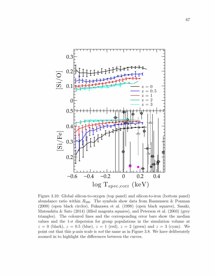
67
0
0.1
0.2
0.3[Si/O]
−0.6 −0.4 −0.2 0 0.2 0.4
0.2
0.3
0.4
0.5
[Si/Fe]
log Tspec ,corr (keV)
z = 0z = 0.5z = 1z = 2z = 3
Figure 3.10: Global silicon-to-oxygen (top panel) and silicon-to-iron (bottom panel)abundance ratio within R500. The symbols show data from Rasmussen & Ponman(2009) (open black circles), Fukazawa et al. (1998) (open black squares), Sasaki,Matsushita & Sato (2014) (filled magenta squares), and Peterson et al. (2003) (greytriangles). The coloured lines and the corresponding error bars show the medianvalues and the 1-σ dispersion for group populations in the simulation volume atz = 0 (black), z = 0.5 (blue), z = 1 (red), z = 2 (green) and z = 3 (cyan). Wepoint out that this y-axis scale is not the same as in Figure 3.8. We have deliberatelyzoomed in to highlight the differences between the curves.

68
of silicon is nearly the same as that locked up in the first place but the amount of
oxygen returned is reduced. The evolution in [Si/O] in Figure 3.10 results from
this differential evolution. As for the gentle rise in [Si/O] with increasing group
temperature, this is a consequence of the four categories in Figure 3.9 not contributing
identically to the silicon and oxygen mass. We emphasize, however, that this increase
with group temperature amounts to maximum change of ∆[Si/O]≈ 0.05, which is
insignificant. For all intents and purposes, [Si/O] is independent of group temperature
or mass.
In contrast, z = 0 [Si/Fe] curve (lower panel) not only increases by ∆[Si/Fe]≈ 0.2
in going from the coolest to the warmest groups in our simulation sample, this change
evolves from ∆[Si/Fe]≈ 0 at z = 3 to its present-day value while the value of [Si/Fe]
in the warmest group drops slightly. To zeroth order, the redshift evolution is due
to delayed Type Ia SNe spewing new forged and winds from AGB stars spewing pre-
viously locked-up iron mass to their local environment. Generally, this environment
is the ISM within the group galaxies. However, transporting this ‘late’ iron out of
the galaxies and into the IGrM is not straightforward. As we have noted previously,
metal-rich winds from the central galaxies in cool groups tend to behave more like
galactic fountains and therefore, very little of the ‘late’ iron production gets into the
IGrM. The central galaxies in the more massive groups are able to drive the iron into
the IGrM but they are not outrightly dominant sources because they are running out
of cold gas and hence, not forming stars as vigorously. Moreover, because of the size
of the galaxies, the mass loading factor of the wind that is ejected is only a fraction
of the star formation rate (c.f., Section 2.1) and even in this case, the ejection of the
‘late’ iron is inefficient. However, winds are not the only way to enrich the IGrM.
Direct enrichment by the IGS component is another. And as illustrated in Figure 3.9,
the latter is the dominant source of iron mass in the cool groups and also the reason
why [Si/Fe] in cool groups evolves much more rapidly than in warm groups.
3.3.4 The Characteristic Timescales for Metal Enrichment of
the IGrM
We conclude our investigation of the metal enrichment of the IGrM by examining the
redshifts by which half of the iron, silicon and oxygen mass in the z = 0 IGrM within
R200 is produced by the stars, regardless of whether the metals are initially deposited
in the ISM or introduced directly into the IGrM. We refer to these characteristic

69
Figure 3.11: The joint distribution of Z0.5 XX,IGrM, the redshift by which half of themetals of species XX=Fe, O, Si in a present-day group’s IGrM has been forged bythe stars/supernova, versus Z0.5 star, the distribution of redshifts by which half of thepresent-day group’s stellar mass has been assembled in its MMP. The contour plotsshow the 2D distribution of the redshifts for the low, intermediate and high massgroups – i.e., 12.5 < log Mvir ≤ 13.0 M (magenta), 13.0 < log Mvir ≤ 13.2 M(blue), and 13.2 < log Mvir ≤ 14.0 M (red) – separately. The inner and the outercontours of the shaded regions of each colour correspond to 1-σ and 2-σ, while the× marks the median for the galaxies in each mass bin. The panels to the left andbelow the contour plots show the normalized marginalized distributions of Z0.5 XX,IGrM
(left), and Z0.5 star (below). The different colour curves show the results for the low,intermediate and high mass groups, and the dashed lines indicate the median.
70
redshifts as Z0.5 Fe,IGrM, Z0.5 O,IGrM and Z0.5 Si,IGrM. We show their distributions in
Figure 3.11, where we compare them to the redshifts by which half of the group’s
z = 0 stellar mass has been assembled in its MMP (Z0.5 star). There are several other
characteristic redshifts, such as the halo formation redshift (Z0.5 halo) or the redshift
at which the hot (T > 5 × 10⁵ K) gas mass in the MMP is half of the group’s final
IGrM mass (Z0.5 IGrM), that we have compared Z0.5 XX,IGrM (where XX=Fe, O, Si)against; however, we do not show these because they do not offer any additional
insights and Figure 3.7 offers a straightforward map between Z0.5 star and the other
potential redshifts of interest.
Examining the timescales in detail, the most significant feature is that in all but
the most recently formed groups, the characteristic ‘metal production’ redshifts are
lower than Z0.5 halo or Z0.5 IGrM. In other words, typically more than half of the iron,
silicon and oxygen in the z = 0 IGrM was forged after half of the groups’ IGrM was
already in place within the nascent groups.
The relationship between Z0.5 XX,IGrM, where XX=Fe, O, Si and Z0.5 star is more
nuanced. In the case of iron (c.f., the top panel of Figure 3.11), the major axis of
the contours has a shallower slope relative to the one-to-one line. Since Z0.5 star is
a measure of when stars first appear inside groups, the orientation of the contours
indicates that the iron in the z = 0 IGrM is typically made after half of the groups’
final stellar mass is in place within the MMP. This is not surprising. As we have
discussed previously, AGB stars and delayed Type Ia SNe play a key role in the
build-up of iron in the IGrM and there is a lag between the formation of a stellar
population and the start of enrichment by Type Ia SNe and AGB stars associated with
that population. However, if this was all, we would have expected the width of the
contours at fixed Z0.5 star to be fairly narrow. Instead, as suggested by the left panel
of Figure 3.9, about 20% of the z = 0 IGrM iron is forged by the stars/supernovae
before the source galaxies become incorporated into groups. In this case, Z0.5 star
registers the stars in these external galaxies only after they fall in; i.e., if they fall in
before z = 0, while the metal production is registered whenever it happens.
Turning to the second panel of Figure 3.11, we see that there is more of a one-
to-one relationship between the timescale for oxygen production and Z0.5 star. This
alignment is the result of two effects acting in concert: (i) Between 60-70% of the
oxygen in the z = 0 IGrM is forged by stars that are already in the groups (c.f., the
right panel of Figure 3.9), and (ii) oxygen production by core-collapse Type II SNe
and transport into the IGrM (by winds) are both tied directly to star formation, with

71
no significant built-in lag between these events.
Turning to the third panel of Figure 3.11, we find that the orientation of the con-
tours in the Z0.5 Si,IGrM−Z0.5 star plot is midway between that of iron and oxygen. As
discussed in the previous subsection, although silicon and oxygen are both produced
in an identical manner, there is one significant difference. AGB stars capture and
retain a non-negligible amount of silicon present in the ISM at the time their progen-
itor stars form, and return it to their surroundings only after a lag time. In effect,
this means that silicon enrichment of the IGrM can proceed via two channels: the
galactic wind and, as is the case with iron, via direct enrichment by the AGB stars
in the IGS. This late-time injection of silicon differentiates the evolution of silicon
from that of oxygen and shifts the distribution of Z0.5 Si,IGrM slightly towards lower
redshifts with respect to the distribution of Z0.5 O,IGrM.
3.4 SUMMARY AND CONCLUSIONS
There is a growing consensus that models of galaxy evolution – or for that matter,
models describing the formation and evolution of galaxy groups and clusters – that
do not allow for large-scale galactic outflows will fail to match the global evolutionary
properties of galaxies. Observations of both local as well as high-redshift galaxies
indicate that not only are large-scale galactic outflows ubiquitous, but that they have
a profound impact on the conditions inside the galaxies as well as conditions in the
wider environment around galaxies. For example, galactic outflows are thought to
play a central role in establishing the observed mass-metallicity relation in galaxies, in
promoting widespread enrichment of the IGM as far back as z ∼ 5, and in accounting
for the abundances and abundance ratios of α and iron-group elements observed in
the hot diffuse X-ray emitting gas in galaxy groups and clusters. Recent observations
as well as theoretical models indicate that AGNs and stars/SNe are both capable
of driving powerful outflows and while definitive observational evidence outrightly
favouring one over the other remains elusive, we argue that only stellar processes are
capable of driving large-scale galactic outflows that can transport a significant fraction
of the metal-enriched ISM out of the galaxies and into their halos and beyond.
Our main findings are as follows:
(i) The distribution of the groups’ formation epochs can be reasonably approxi-
mated by a Gaussian with a median of z ∼ 1 and σ = 0.4. Moreover, the epoch when
half of a present-day group’s X-ray emitting, intragroup medium (i.e. the diffuse halo

72
gas with T > 5 × 10⁵ K) is in place is tightly correlated with the group’s formation
epoch. Examining the emergence of the latter in more detail, we find that in halos
with gravitational potential wells of a given depth, the median IGrM mass fraction
increases with time prior to z ≈ 1 as the halos recapture the gas that was expelled
out of the galaxy-scale halos at earlier epochs, (the ratio of baryons-to-dark matter of
the infalling material is larger than the universal value) and most of these baryons are
shock-heated to roughly the virial temperature of the groups upon accretion. After
z ≈ 1, the IGrM fractions within R200 cease to increase with time because the IGrM
is sufficiently extended that the newly accreted (and thermalized) baryons primarily
remain at r > R200 and become part of this extended halo gas distribution. Apart
from this trend with time, the IGrM mass fractions within R200 also increase with
halo mass at all epochs. This increase is the result of the larger mass systems hav-
ing deeper potential wells and higher virial temperatures. Consequently, more of the
diffuse gas is shock-heated to constitute the IGrM and the deeper potentials confine
this gas more effectively.
(ii) Our stellar-powered, momentum-driven wind model yields X-ray scaling re-
lations that are in excellent agreement with observed scaling relations (e.g. X-ray
luminosity-temperature, mass-temperature, entropy-temperature, etc.) over much of
the regime associated with galaxy groups despite the fact that the model does not
include AGN feedback. These scaling relations evolve self-similarly from z = 1 to
the present, as does MIGrM,200/M200 versus M200. The hot, diffuse, X-ray emitting,
intragroup gas is not subject to catastrophic cooling. Typically only a percent or less
of z = 0 IGrM mass is lost via cooling over a Hubble time. We do, however, see a
tendency for the simulated galaxy groups to be slightly more X-ray luminous and/or
have slightly cooler X-ray spectroscopic temperature than the observed groups on
mass scales M500E(z)>∼1014 M. At face value, these results collectively suggest that
AGN feedback is not necessary to understand the properties of the hot diffuse gas in
the simulated groups until the halos approach cluster-scale.
(iii) Our simulation also successfully reproduces both the observed, spatially re-
solved, mass-weighted as well as the observed, unresolved, emission-weighted IGrM
silicon and iron abundances within R500. This agreement also includes the observed
trend of [Fe/H] and [Si/H] increasing with temperature until ∼ 1 keV and then flat-
tening. Probing the origin of the metals in the IGrM in more details, we find that
nearly 50% of the IGrM silicon, oxygen and iron mass in our simulated groups are

73
produced in the central and the satellite galaxies of a present-day group or its MMP,
and infused into the IGrM via galactic outflows, while between ∼ 12% (oxygen) to
∼ 30% (iron) is transferred to the IGrM via direct enrichment by the IGS.
(iv) Turning our attention to the group galaxies, we find that the stellar-powered,
momentum-driven wind model results in a present-day stellar mass function for group
galaxies that is in excellent agreement with the observations for M∗ < 1011 M;
however, we also find galaxies – typically, one per group and invariably, the group
central galaxy – that have much larger stellar masses than any observed galaxy. These
are the galaxies that are responsible for the elevated stellar and total baryonic mass
fractions in our simulated groups. Artificially reducing the stellar mass in only these
‘large’ galaxies by a factor of ∼ 3 reconciles the group stellar mass fractions with the
observations across the entire mass range 12.5 ≤ log(M∗) ≤ 14.0.
(v) The excess stellar mass in these ‘large’ group galaxies is due to galaxies no
longer being able to moderate their star formation rates by depleting their cold gas
mass via expulsion once they grow larger than M∗ ≈ 4 × 10¹⁰ M. The deepening
gravitational potential of these galaxies and a higher cross-section for hydrodynamic
interactions between the galactic outflows and the shock-heated halo gas component,
once the latter starts to form, confine the wind material within the circumgalactic re-
gion. Being metal-rich, most of this wind material cools down and falls back into the
galaxy in a manner more akin to galactic fountains rather than outflows (c.f., Oppen-
heimer et al., 2010). The high cold gas mass in our group central galaxies is largely a
consequence of this, and the overproduction of stars is a byproduct. The breakdown
of the stellar-powered winds model in our giant group galaxies generally occurs before
the galaxies are incorporated into bonafide groups and is the earliest indication that
another feedback mechanism, like AGN feedback, is needed.
(vi) We assert that in large galaxies, at least, AGN feedback cannot simply act to
heat the halo gas just enough to offset the radiative cooling losses. This maintenance-
mode or hot halo quenching feedback may represent a reasonable description of how
AGN feedback operates in galaxy clusters and may even result in ‘large’ galaxies with
realistic stellar properties (c.f., Gabor & Dave, 2012, 2015, and references therein),
but because this type of feedback is, in effect, only shifting baryons in our simulated
groups from the galaxies to the IGrM component, the total baryon fraction of the
groups will not change. Our simulated groups, however, already have too high a
74
baryon fraction (c.f., Figure 3.5). At the same time, the IGrM mass fractions will
become more discrepant and a denser IGrM means that the simulated groups of a
given mass will be more X-ray luminous than their observed counterparts. To ensure
that both the stellar masses of the ‘large’ galaxies and the hot gas properties of the
groups agree with observations, AGN feedback (or for that matter, any new feedback
mechanism or combination of mechanisms) must step in when stellar feedback starts
to fail and continue to drive outflows beyond the galactic halos and perhaps even,
beyond the low mass group halos.
(vii) Finally, we emphasize that we do not expect the inclusion of AGN feedback,
and the expected reduction in the stellar mass within the groups, to alter the agree-
ment between our simulation results and the observed IGrM metal abundances (and
abundance ratios) in galaxy groups. Even after discounting the metals produced by
2/3 of the stars in the ‘over-sized’ galaxies, the absolute abundances in the simulation
are still consistent with the observations, especially when one accounts for the factor
∼2 uncertainty in the adopted nucleosynthesis yields and supernova rates.

75
Chapter 4
THE ENRICHMENT OF THE
IGRM - HOW? WHERE? WHEN?
In this chapter, we focus specifically on how the enrichment of the IGrM proceeds.
In Section 4.1, we describe the present-day IGrM metal abundance profiles in the
simulated groups, compare these to observations, and examine how these profiles
have evolved over cosmic time. In Section 4.2, we explore where and when the IGrM
metals at different radii of today’s groups were forged by the stars/supernovae, and
when and where these metals entered the hot gas phase. We also identify the sources
of these metals and their relative contributions. And finally, we discuss and summarize
our findings in Section 4.3.
4.1 Radial profiles
As noted in the Introduction, the metal content in the IGrM represents a record of
the various astrophysical processes associated with the formation and evolution of
galaxies in the dense group and cluster environments. In Chapter 3, we computed
the mean mass-weighted IGrM iron (ZFe) and silicon (ZSi) abundances within R500
of simulated z = 0 groups with core-corrected spectroscopic temperatures ranging
from 0.25 keV to 2.25 keV, and compared these to available observations. We find
that the amplitude and the scaling of ZFe and ZSi with Tspec,corr in both the simulated
and observed groups are in very good agreement with each other (c.f., Figure 11 of
Chapter 3). Specifically, we find that both ZFe and ZSi rise steeply with temperature
for systems with Tspec,corr <∼ 1 keV and then flatten. In this section, we explore the
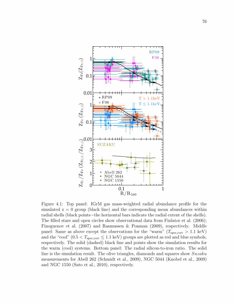
76
0.1 10.01
0.1
1
ZFe(ZFe,⊙)
0.1 10.01
0.1
1
ZFe(Z
Fe,⊙)
0.1 10
1
2
3
R/R500
ZSi/ZFe(Z
Si,⊙/ZFe,⊙)
Abell 262NGC 5044NGC 1550
SUZAKU
⋆ RP09 F06
RP09
F06
T > 1.1keV
T ≤ 1.1keV
Figure 4.1: Top panel: IGrM gas mass-weighted radial abundance profile for thesimulated z = 0 group (black line) and the corresponding mean abundances withinradial shells (black points−the horizontal bars indicate the radial extent of the shells).The filled stars and open circles show observational data from Finlator et al. (2006);Finoguenov et al. (2007) and Rasmussen & Ponman (2009), respectively. Middlepanel: Same as above except the observations for the “warm” (Tspec,corr > 1.1 keV)and the “cool” (0.5 < Tspec,corr ≤ 1.1 keV) groups are plotted as red and blue symbols,respectively. The solid (dashed) black line and points show the simulation results forthe warm (cool) systems. Bottom panel: The radial silicon-to-iron ratio. The solidline is the simulation result. The olive triangles, diamonds and squares show Suzakumeasurements for Abell 262 (Schmidt et al., 2009), NGC 5044 (Knobel et al., 2009)and NGC 1550 (Sato et al., 2010), respectively.

77
spatial distribution of ZFe, ZSi and ZO within the simulated z = 0 groups, and
compare these with the observations. We then describe how these abundance profiles
have evolved over time.
4.1.1 Abundance Profiles at present
The top panel of Figure 4.1 shows the mean mass-weighted spherically-averaged, ra-
dial profile of the mass-weighted radial IGrM iron abundance, ZFe(r), in the simulated
z = 0 groups with Tspec,corr > 0.5 keV (black line), and the mean abundances within
radial shells (black points) at different distances from the group centres, scaled by
R500 (z = 0). The latter not only facilitates the stacking of the simulated groups
but also comparison with the observations. The width of the horizontal “error bars”
indicates the size of radial bins within which the mean abundances are determined.
Filled magenta stars and green circles are observational results for the mean mass-
weighted ZFe in radial shells from Finlator et al. (2006); Finoguenov et al. (2007)
and Rasmussen & Ponman (2009), respectively. We have scaled the radius of the
shells for observed groups to R500 derived from the R500 − Tspec,corr relationship for
the simulated groups.
The large scatter in the data notwithstanding, the observed ZFe(r) declines from
the value of ∼ 0.3Z in the innermost bins (r < 0.1R500) to just under ∼ 0.1Z at
∼ 0.7R500. Overall, the simulation abundance profile is in reasonably good agreement
with the observations, especially the more recent Rasmussen & Ponman (2009) data.
In detail, the simulation profile is a bit steeper than the observed profile. One reason
for this is that the catalog of simulated groups is much more skewed towards lower
temperature groups compared to the observational samples, and the lower tempera-
ture simulated groups tend to be more metal rich in the central regions than observed
groups of comparable temperatures. This is illustrated in the middle panel where,
following Rasmussen & Ponman (2009), we show the same observations as in the top
panel but color-coded so that the results for the “warm” groups (Tspec,corr > 1.1 keV)
are shown in red, and those for the “cool” groups (0.5 < Tspec,corr ≤ 1.1 keV) are
in blue. The results for the “warm” and “cool” simulated groups are illustrated by
the solid and dashed black lines and points, respectively. The simulation and obser-
vational results for the warm groups are in very good agreement, although one can
argue that the innermost regions of even the “warm” simulated groups are slightly
more metal rich. In the case of the “cool” groups, the difference in the metallicity

78
in the innermost shell grows to a factor of ∼ 2. This central iron excess, restricted
as it is to a small fraction of the volume, does not impact the global ZFe within R500
(c.f., Chapter 3).
The elevated IGrM abundance in the central regions of the simulated groups is
directly linked to the star formation in the central galaxies in the groups. In Sec-
tion 4.2 of the present paper, we examine when and where the metals at different radii
in the present-day groups come from and show that metals in the IGrM in the central
regions primarily originate in the central galaxies (c.f., Figure 4.3). In Chapter 3, we
showed that the current simulation results in these central galaxies having too many
stars. Squelching star formation through the introduction of additional mechanisms,
like AGN feedback, should lower the abundances in group centres. Moreover, any ra-
dial transport of metals from the group centre to larger radii, even if not a dramatic
effect, by turbulence and bulk motions induced by AGN-powered outflows, and by
drifts and wakes associated with buoyantly rising, AGN-inflated bubbles (c.f. Pope
et al. 2010 for a theoretical discussion of bubble wakes and drifts, McNamara et al.
2014 and Russell et al. 2014 for potential observational evidence for mass uplift and
Revaz, Combes & Salome 2008 for related numerical simulations) will tend to make
the IGrM abundance profile slightly less steep (c.f., McCarthy et al., 2010) and fur-
ther improve the agreement between the simulation results and the observations. We
expect these effects to be more pronounced in groups with shallower potential wells.
In the bottom panel, we compare the radial profile of the mean mass-weighted
silicon-to-iron ratio (ZSi/ZFe) for the simulated z = 0 groups (black line) with the
Suzaku measurements (olive symbols) for Abell 262 (Schmidt et al., 2009), NGC
5044 (Knobel et al., 2009) and NGC 1550 (Sato et al., 2010). The silicon-to-iron
ratio in both the observed and the simulated groups is largely flat from the group
centre out to R500 although on closer examination both exhibit a very gentle drop with
increasing radius. The two are, however, offset from each other such that the ratio in
the simulated groups is ∼ 30% larger. Focusing first on the gradient with radius, the
slightly elevated ZSi/ZFe in the central region occurs because of a mild drop in the
IGrM iron mass there relative to the other metals. Iron is an efficient coolant and
gas that is rich in iron tends to cool and drop out of the IGrM phase on a slightly
shorter timescale. As for the offset, there are potentially three ways of adjusting the
simulation parameters to resolve this discrepancy: Reduce the Type II SNe silicon
yield; increase the production of iron through a higher Type Ia SNe rate; raise the
Type Ia/II iron yields; or some combination thereof. We don’t think that reducing

79
the silicon yield (alone) is the solution. We showed in Chapter 3 that although ZSi
within R500 in the simulated groups is in agreement with the observations. It is,
in detail, slighly on the low side. If the silicon yield in the simulations were to be
reduced, the spread between the observations and the simulated results would grow
larger. Our comparison favours a slightly larger silicon yield than the one used in
the simulations. On the other hand, if the iron production were to increase, not only
would the agreement between the simulation results for the global ZFe within R500 and
the observations improve (c.f., Chapter 3), the simulated and observed silicon-to-iron
ratio would also come into better agreement. Given that even for a fixed IMF, there
is still a factor of ∼ 2 uncertainty in the nucleosynthesis yields and supernova rates,
it is not inconceivable that the correct yields and rates could result in a ∼ 30% more
iron mass in the IGrM.
4.1.2 The evolution of metal profiles
Next we examine how the metal distribution in the IGrM evolves over cosmic time.
In the top panel of Figure 4.2, we show the mean spherically-averaged radial pro-
files of the mass-weighted iron abundance in the IGrM of the simulated groups with
Tspec,corr > 0.5 keV at selected redshifts 0 ≤ z ≤ 3. We have omitted similar plots for
silicon and oxygen because to first order, the shapes of the corresponding abundance
profiles at the redshifts under consideration are similar to those of iron. Specifically,
the abundance profiles of all three elements at the earliest time shown (z = 3) indicate
an enhancement in the inner 0.3R500 and a long flattened plateau (corresponding to
ZFe ≈ 0.02ZFe, for iron) that extends past 4R500 (≈ 2Rvir). The latter is the result
of the winds from the early galaxies in the proto-group regions expelling a significant
fraction of their metal-enriched ISM over regions extending well beyond R200 of the
z = 3 groups. We have shown in Chapter 3 that these powerful early outflows also
lead to the significant reduction (∼ 75%) of the baryonic mass fraction within 6R500
(≈ 3Rvir), with respect to the cosmic mean value, in the early groups at z = 3 as well
as elevate the metallicity of the affected intergalactic gas. The central enhancement
is due to the outflows from groups’ central galaxies.
Between z = 3 and z = 1, the abundance profiles interior to R500 (≈ 0.5Rvir)
steepen and the amplitude of the extended tail declines. We note that this period is
also characterized by the growth of the groups’ baryonic mass fraction, from ∼ 75%
to ∼ 90% of the cosmic mean (c.f., Chapter 3). The above two trends are due to the

80
0.1 1
0.01
0.1
1ZFe(Z
Fe,⊙)
z=0z=0.5z=1z=2z=3
1.5
2
2.5
3
3.5
ZSi/ZFe(Z
Si,⊙/ZFe,⊙)
0.1 10.5
1
1.5
2
ZSi/ZO(Z
Si,⊙/ZO,⊙)
R/R500
Figure 4.2: Mass-weighted radial profiles of the IGrM iron (top panel) abundance,silicon-to-iron ratio (middle panel), and silicon-to-oxygen (bottom panel) of the sim-ulated groups at z = 0 (black), z = 0.5 (blue), z = 1 (red), z = 2 (green) and z = 3(cyan).

81
same evolutionary processes: (1) The previously expelled metal-enriched material is
re-accreted by the growing groups and the gas on successively larger scales is replaced
by less enriched intergalactic medium, and (2) the newly expelled gas from the group
galaxies is confined to a decreasing fraction of Rvir(z), with the intra-group spatial
gradient arising due to the groups’ central galaxies dominating the enrichment of the
inner regions.
Below z ≈ 1, the abundance profiles continue to steepen, but at a slower rate.
This is, in part, because a significant fraction of the previously expelled metal-enriched
gas by the early galaxies has been (re)incorporated into the groups; in part, because
declining star formation in the central galaxies results in reduced outflows; and, in
part, because the cooling of the metal-rich, dense gas in the central regions of the
groups become sufficiently rapid that it partially counteracts the enrichment of the
IGrM due to the winds from the central galaxies and the intra-group stars. (Note
that this does not contradict with the statement in Chapter 3 that only a few per cent
of the hot IGrM is lost due to cooling over cosmic time in that the limited amount of
cooled IGrM is highly-enriched and therefore metal loss from the IGrM is significant.)
In detail, there are in fact differences in how the metal abundances of different
metal species evolve. In the middle and the bottom panels of Figure 4.2, we show the
mean radial profiles of the silicon-to-iron (ZSi/ZFe) and the silicon-to-oxygen (ZSi/ZO)
mass ratios, respectively, in the IGrM of simulated groups at various redshifts. Prior
to z ∼ 2, both the ZSi/ZFe and ZSi/ZO profiles primarily reflect the yield ratios and
relative rates of the Type II SNe and the prompt component of the Type Ia SNe.
At lower redshifts, the metals from the delayed Type Ia SNe and the AGB stars
become increasingly important. The silicon-to-iron ratio, for example, declines from
2.75 solar at z > 2 to 2.3 − 2.4 solar. This drop is entirely caused by the increase
in the iron mass due to the delayed Type Ia SNe. Moreover, since the Type Ia SNe
produce negligible amount of silicon, the magnitude of the change implies that the
delayed Type Ia SNe are responsible for ∼ 15% of the total iron in the present-day
IGrM. The AGB stars do not alter the abundance of iron or silicon.
The evolution of ZSi/ZO, on the other hand, is entirely due to the AGB stars.
While these neither produce nor destroy silicon, the same is not true of oxygen. They
both produce and destroy oxygen, with the overall effect being a net decrease in
the oxygen mass. Consequently, the mass ejected from the AGB stars has a higher
silicon-to-oxygen ratio than that of the gas from which the AGB stars were formed
(see OD08). The late time increase in the IGrM ZSi/ZO is the direct consequence of

82
this.
4.2 Dissecting the enrichment of the IGrM
Having established how the IGrM metal abundances grow with time, we now inves-
tigate in detail how this enrichment occurs. We determine the extent to which the
various sources of the metals — the central galaxy, the satellite galaxies, the external
galaxies and the intra-group stars (IGS) — contribute to the metallicity at different
radii within the present-day group halos, and establish when and where the metals
are forged by the stars/supernovae and injected into the IGrM. The approach de-
scribed here is based on the approach used by Crain et al. (2013) to investigate the
enrichment of the hot/warm gas that cocoons the galaxies.
4.2.1 The origin of the IGrM metals
Our simulation generates approximately 60 outputs (“snapshots”) spanning the red-
shift range from z = 10 to z = 0, and information, such as position, velocity, metal
abundances (for SPH and stellar particles) and etc, of all SPH+stellar+dark matter
particles in the simulation is recorded at every snapshot. We select the IGrM parti-
cles of the simulated z = 0 groups and track them back in time using the unique ID
assigned to each particle in the simulation. For a given gas particle, if there is metal
mass increment between two successive snapshots, we flagged the particle as having
been enriched. Like what we have done in Chapter 3, based on the status of the
particle at the time of enrichment, we identify the potential site of metal production
as follows:
Central: The central galaxy of the present-day group or the central galaxy of the
group’s most massive progenitor (MMP) at an earlier epoch.
Satellite: A non-central galaxy that is contained within the z = 0 group halo or
within the group’s MMP.
External: A galaxy that is neither a central nor a satellite at the time of enrich-
ment.

83
IGS: Direct enrichment of the IGrM by intra-group stars (i.e., stars in the present-
day group or any of its progenitor subhalos that are not bound to any of
the skid-identified galaxies) as well as the enrichment associated with the
unresolved galaxies (i.e., Mtot <∼ 2.9× 10⁹ M). 1
We construct each group halo’s merger history using its dark matter particles and at
each point in time, and identify the most massive halo in tree as the MMP. Within
each group, the most bound galaxy (i.e., the galaxy that has the lowest total gravita-
tional potential energy, accounting for both self-gravity as well as the gravity exerted
by all the baryonic+dark matter within the simulation volume) is said to be the cen-
tral galaxy of the group and likewise, we define the most bound galaxy within the
MMP.
We note that since we only save a finite number of simulation outputs, the precise
moment of enrichment will not correspond to the redshifts of the recorded snapshots.
We therefore identify the enrichment environment based on the location of the gas
particles at the two consecutive snapshots that bracket the enrichment event. Specif-
ically, if at either one of the two snapshots, a gas particle is associated with a galaxy,
we assume that that galaxy is responsible for the enrichment. On rare occasions, a
gas particle may be associated with two different galaxies in the two snapshots. Such
cases arise when two galaxies merge during intervening time. In these instances, we
assign the enrichment to the snapshot with the more massive galaxy. This is different
from the approach adopted by Crain et al. (2013), who classify enrichment events
based only on the snapshot preceeding the enrichment event, because we also want to
apply tight constraint on the enrichment associated with the IGS component, which
Crain et al. (2013) do not explicitly account for in their study on the circum-galactic
medium. In our study, we assume the enriched gas particles that have no galaxy ID
at either of the two bounding snapshots to be enriched by the IGS.2 We also note
that the sampling in our post-run analysis is sufficient for the classification of the en-
1In this chapter, we define the IGS in a slightly different manner compared to what we have donein Chapter 3, such that the IGS here includes the stars that are bound to the unresolved galaxies.The new definition is valid in that the boundary between these unresolved objects and the real fieldstars is intrinsically ambiguous, and also they contribute very limited amount of metals to the IGrMwithin R500.
2We also exclude the enrichment events that meet this criteria but where the enriched gas particleis identified as wind between the two consecutive snapshots bracketing the event. We associate theseparticles as having been enriched by the “galaxies” identified by the in-situ finder but not by thepost-run finder. We find that the metal mass associated with these wind particles only accounts for∼ 5% of the total metal mass linked to the “IGS” category by the initial criteria.

84
0.2
0.4
0.6
0.8
1
Zx/Zto
t
0.1 10
0.2
0.4
0.6
0.8
1
Zx/Zto
t
0.1 1
0.1 10.1 1R/R500 (z = 0)
Fe Si O
Satel l i te
Central
ExternalIGS
Figure 4.3: Top panels: Mass fraction of the metals in the present-day IGrM con-tributed by various enrichment sources: central (red), satellite (magenta), and ex-ternal galaxies (blue), as well as the IGS (orange), as a function of the present-daydistance of the metals from the group centre. The left, middle and right panels showthe results for the three different metal species. Bottom panels: The classificationof the enrichment is different from that used by the top panels, in the sense thatfor those metals that were ejected from a galaxy, it is based on the site of the mostrecent ejection. The solid and the dashed lines represent results for the warm andcool groups, respectively.
richment sources since our results do not change significantly even when our tracing
algorithm uses only every second snapshot. We ignore the tiny fraction of the metals
synthesized before z = 10.
In the top panels of Figure 4.3, we show the radial profiles for the fractional
contribution by each of the four enrichment sources to the total iron (left), silicon
(middle) and oxygen (right) mass in the IGrM of the present-day groups. The results
for the warm and cool groups are explicitly shown by the solid and the dashed curves,
respectively. Also in Figure 4.4, we show the integrated fractional contribution by
the various sources over three radial bins: 0 ≤ r < 0.1R500 (left column), 0.1R500 ≤r < R500 (middle column), and R500 ≤ r < 1.5R500 (right column). The odd and
even rows of the pie charts correspond to the results for the the warm and cool
groups, respectively. We will at first describe the general features for the entire group

85
59%13%
10%
18%0 ï 0.1R500
30%
17%18%
35%
0.1 ï 1R50022%
15%
24%
38%
1 ï 1.5R500
56%
9%
13%
22% 25%
13%
16%
46%
17%
12%
21%
50%
Fe(warm)
Fe(cool)
60%14%
11%
15%32%
20% 21%
27% 25%
17%
28%
30%
58%
10%
14%
18%30%
16%20%
34%21%
15%
26%
39%
Si(warm)
Si(cool)
54%
17%
16%
14%30%
21% 26%
24% 23%
18%
33%
26%
53%
12%
19%
16%29%
17% 25%
29%20%
16%
31%
33%
CentralSatel l i teExternalIGS
O(warm)
O(cool)
Figure 4.4: The metal budget of the present-day IGrM within different radial bins:0−0.1R500 (left column), 0.1−1R500 (middle column), and 1−1.5R500 (right column),split by various enrichment environments: central galaxies (red), satellite galaxies(magenta), external galaxies (blue) and IGS. The results for the three different metalelements and the warm and cool groups are separately shown as labelled.

86
population and then turn to the difference between the warm and cool groups.
Focusing at first on the galaxy-associated categories (i.e., “Central”, “Satellite”
and “External”) in the top panels, it is apparent that the “Central” category (red)
dominates the enrichment of the IGrM over any of the other two from the group
centre out to ∼ R500 (∼ 0.8 − 1R500 for the iron and silicon and ∼ 0.5 − 0.6R500 for
the oxygen), beyond which the “External” category (blue) becomes dominant. The
“Satellite” category (magenta) plays an important but sub-dominant role, accounting
for nearly constant 10%− 20% of the total metal mass over 0− 2R500. The variation
of the fractional contributions with r(z = 0) is also clearly demonstrated by the pie
charts in Figure 4.4: In both warm and cool groups and for all three metal species,
the central galaxies in the groups and their MMPs dominate over the satellite and
external galaxies for the two inner radial bins, whereas for the other bin, the external
galaxies are the most important contributors.
Comparing the enrichment style between the three different elements, it can be
seen that the relative contribution to the iron and silicon in the IGrM by the three
galaxy-related categories is very similar (The ratio between the three categories is
observed to be similar by comparing the corresponding pie charts in the first two
and the middle two rows in Figure 4.4). This is because in our simulation, the
enrichment that takes place in the dense star forming regions within the galaxies
is dominated by the combined yields from the Type II SNe and the prompt Type
Ia SNe (the rate of both being scaled to the SFR), whereas the delayed Type Ia
SNe (their rate being scaled to stellar mass) contribute a smaller fraction, and hence
the iron-to-silicon ratio of the galaxy-associated enrichment is not sensitive to the
stellar populations (galaxy types). Were it not for processing by the AGB stars, we
would expect the oxygen to shows the same trend. However, there is hint that the
“Central” (“External”) category plays relatively less (more) important role in oxygen
production compared with the iron or silicon: The ratio of the “Central” (“External”)
to the “Satellite” for the iron within 0.1R500 in the warm groups (top left pie chart)
is 59%13%
= 4.54 (13%10%
= 0.77), while for the oxygen within the same radial bin (the left
of the fifth row), 54%17%
= 3.18 (16%17%
= 0.94). This indicates that the ISM of the central
(external) galaxies is more (less) subject to the AGB processing, in the sense that
a larger (smaller) fraction of the oxygen mass was burned through the AGB stars.
This is not surprising, as the ISM in the more massive galaxies is “chemically older”,
in the sense that the ISM has been subject to more frequent recycling as a result
of these galaxies having deeper gravitational wells and because their circumgalactic

87
environment consists a dense gaseous halo (c.f., Oppenheimer et al., 2010, Liang
et al. 2015). Therefore, the gas enriched within the relatively more massive central
galaxies is characterized by a lower oxygen-to-iron ratio than that associated with the
satellites, whereas the gas enriched within the relatively less massive external galaxies
exhibits a higher ratio.
Turning to the “IGS” category (orange), we find that the diffuse, unbound stars
are important contributors of iron to the present-day IGrM. The “IGS” category is
expected to be characterized by lower α-to-iron ratio than the galaxy-related cate-
gories since there is no ongoing star formation in the intra-group environments and
the enrichment associated with the field stars should be primarily due to the metals
from the delayed Type Ia SNe and the AGB stars. Indeed, we do see from the top
three panels of Figure 4.3 as well as in Figure 4.4 that the “IGS” category accounts for
a relatively smaller fraction of the α-element (silicon and oxygen) mass in the IGrM
than the iron mass. The silicon and oxygen yields for the Type Ia SNe are almost
negligible in our cosmic chemical model, and any contribution to these two elements
by the “IGS” category should be primarily due to the mass loss from the AGB stars
in the field. The metallicity of the wind from the AGB stars is that of the progenitor
ISM from which they were spawned, modified by any processing that occurs in the
stars during their lifetime. Specifically, oxygen burning within the AGB stars results
in a lower fractional return of the oxygen mass in comparison to the silicon mass.
Comparing the results for the warm (solid) and cool (dashed) groups in Figure 4.3,
we can see that in the cool systems, the IGS contributes relatively more of the metals
(especially iron) in the present-day IGrM while the contribution by the galaxies is
correspondingly weaker. This is because in the cool systems, transporting the more
recently produced metals out of the galaxies (especially the central galaxy) is more
difficult as the metal-rich outflows do not travel very far from the galaxies and when
they are halted, they shock-heat to temperatures coinciding with the broad peak in
the cooling curve, cool rapidly and fall back into the galaxies. In the warm systems,
outflows are more energetic and a larger fraction of them shock-heat to temperatures
beyond the broad peak where cooling rate becomes comparatively low. A larger
fraction of the ejected metals in the cool groups end up in the cold phase (ISM or
stars) than in the warm groups.
For the gas that is enriched and flushed out of the galaxies and into the IGrM by
galactic outflows, the “environment” in which it is enriched need not to be the same
as the one it is expelled from. For instance, let us consider the case of an initially

88
70%
12%
2%
16%
0 ï 0.1R500
37%
22%8%
32%
0.1 ï 1R500
29%
21%15%
36%
1 ï 1.5R500
68%9%
4%
20%32%
17% 8%
43%
22%
16%
14%
48%
Fe(warm)
Fe(cool)
72%
13%
3%12%
41%
25%
10%
24%32%
24%17%
28%
71%
9%
4%
15%
39%
20%10%
31% 27%
20%18%
35%
Si(warm)
Si(cool)
71%
16%
4%8%
40%
28%
13%
20%31%
26%
21%
22%
69%
11%
6%
14%
40%
23%
13%
24% 28%
22% 21%
30%
CentralSatel l i teExternalIGS
O(warm)
O(cool)
35%
13% 11%
37%
4% 3%3%4%
84%
6% 1%2%4%
73%
20%
34%
12%15%
30%
10% 2%2%3%
81%
12%< 1%1%
2%
62%
34%
CentralSatel l i teExternalIGSPristine
IGrM(warm)
IGrM(cool)
Figure 4.5: The top six rows of pie charts show the metal budget of the present-day IGrM within
the four radial bins, classified according to their location at the time when they were injected into
the IGrM. The color scheme is the same as that in Figure 4.3. The results for the three different
metal elements and the warm and cool groups are explicitly shown. The two bottom rows show
the mass fraction of the IGrM that has been injected from the central (red), satellite (magenta)
and external (blue) galaxies. The orange segments illustrate the fraction of the IGrM that was not
released from galaxy, but has non-primordial metal abundances. This is gas predominantly enriched
by the IGS. The green segments represent the pristine gas with primordial abundances (i.e., X=0.25
and Y=0.75).
89
“external” galaxy that at a later time is incorporated into a group and becomes
a “satellite”. Some of the metals produced while the galaxy is an “external” may
enter the IGrM after the galaxy becomes a “satellite galaxy”. In the lower panels of
Figure 4.3, we show the fractional contribution of the present-day IGrM metals by
various categories but here the classification is based on the local conditions at the
time when redthe metals were ejected into the IGrM. Also in Figure 4.5, we show
the integrated fractional contributions by these categories over the same radial bins
adopted in Figure 4.4 and separately present the results for the warm and cool groups
as well as the three different elements as labelled.
Comparing the top and bottom panels of Figure 4.3, it is immediately apparent
that the amount of metals ejected from one class of galaxies is considerable different
from the amount synthesized within the same category. For example, we can see
that over r = 0 to r = 2R500, the amount ejected from the central and satellite
galaxies is higher than that synthesized within these galaxies, whereas for the external
ones, the former is lower. Comparing the corresponding pie charts in Figure 4.4 and
Figure 4.5, we find that for the warm groups (odd rows), the difference between the
two classifications for the central galaxies amounts to 11% (12% vs. 16%), 7% (9%
vs. 10%), and 5% (6% vs. 8%) of the total iron (silicon vs. oxygen) mass within
0 ≤ r < 0.1R500, 0.1R500 ≤ r < R500, and R500 ≤ r < 1.5R500, respectively. The
difference for the cool groups is very similar. These numbers refer to the amount
of metals that were synthesized by the stars out of the central galaxies but later
entered (via galaxy merger) and were flushed out of the central galaxies through
outflows. The trend of decreasing discrepancies between the two classifications with
increasing r(z = 0) is due to the fact that the wind particles at larger r(z = 0) were
on average ejected at earlier epochs, as we will discuss in more detail in Section 4.2.2.
This fact, in turn, indicates that they have less chance of being enriched by some
early non-central galaxies. For the satellite galaxies, we find that the amount of iron
(silicon, oxygen) injected from these systems into the IGrM is higher than the amount
injected by the stars within them. For the warm groups, the difference is < 1% (1%
vs. 1%), 4% (4% vs. 6%), and 6% (5% vs. 6%) of the total iron (silicon vs. oxygen)
mass within the three chosen radial bins. These discrepancies are attributed to the
amount of the metals synthesized by the stars within some external galaxies and the
unbound field stars outside of the MMP. The mass of these metals surpasses that of
the metals generated within the satellites but later ejected from the central galaxies
after merger. Comparing the first column of the two figures, it can be seen that in

90
the innermost regions (r ≤ 0.1R500), the metals produced inside the external galaxies
are barely ejected directly from those galaxies. At 0.1R500 ≤ r < R500, more than
half of the metals injected from the stars within the external galaxies were ejected
into the IGrM after the galaxies became incorporated into the MMP. The external
galaxies only become the dominant source of the IGrM metals in the z = 0 groups at
r >∼ 1.5R500 (≈ R200), with regards to the the local conditions at the time when the
metals entered the IGrM.
It should be noted that the “IGS” category (orange) in the lower panels of Fig-
ure 4.3 (also in Figure 4.5 for the integrated results) does not include those metals
that were at first injected from the IGS, but later accreted onto and ejected from a
galaxy. They are instead classified to the category associated with that galaxy from
which they were ejected into the IGrM. In other words, the “IGS” category in the
top panels (also in Figure 4.4) is expected to account for a larger fraction of the total
metal mass than that in the lower ones (also in Figure 4.5).
The last two rows of pie charts in Figure 4.5 show the mass fraction of the IGrM
divided by the various categories as labelled. The red, magenta and blue segments
show the fraction of the IGrM that has been processed (enriched while bound) and
ejected by the central, satellite and external galaxies, respectively. Like in the pie
charts above, the particles that have been ejected by multiple times as wind are clas-
sified based on the last ejection event right before they entered the IGrM. We can see
that the processed IGrM accounts for a decreasing fraction of the total IGrM mass
with increasing r(z = 0) — within the four selected radial bins, from the center to
the outskirt, the processed IGrM accounts for 59%, 10%, 7% and 5% of the IGrM
mass in the warm groups, and 60%, 7%, 4% and 3% in the cool groups. That the
distribution of the metal-rich processed wind material in the present-day IGrM is
more concentrated towards the group center than that of the overall IGrM mass is
one important (but not the only) reason for the groups’ abundance gradients (see
Figure 4.1). Except in the most inner radial bin (r < 0.1R500), the processed IGrM
merely accounts for a few percent of the total IGrM mass, while the majority of the
IGrM has never ever been processed by any galaxy over cosmic time. Comparing the
corresponding pie charts in the last two rows, we find that the cool groups contain
a smaller fraction of the processed IGrM. This is, in part, due to relatively more
efficient radiative cooling of the metal-rich, wind material ejected from the central
and the satellite galaxies in the cool groups. Apart from that, because of the rela-
tively shallower potential wells and weaker viscous drag in less dense environments,

91
the galaxies within and surrounding the cool groups ejected the outflows to further
distance (in terms of the virial radius of the group) from the group center at early
epochs, before they became incorporated into the groups. More of the ejected parti-
cles from those galaxies end up in the intergalactic environments by the present day.
The higher mass fraction of the processed IGrM in the z = 0 warm groups results in
their exhibiting higher metal abundance profiles compared to the z = 0 cool groups
(see the middle panel of Figure 4.1).
The wind material ejected from the different types of galaxies has distinct metal
abundances. From Figure 4.5, it can be seen that the central (external) galaxies
contribute comparatively more (fewer) metals per unit gas mass. For example, within
0.1R500 of the warm groups (see the left panel of the second last row), 35% of the
IGrM was ejected from the central galaxies, and it contains 70% of the total iron
in that region (see the top left panel). The gas ejected from the satellite galaxies
accounts for 13% of the total IGrM mass, yet this portion of gas only contains 12%
of the total iron. For the external galaxies, 11% of the total IGrM containing only
3% of the total iron mass.
Figure 4.6 shows the histograms for the number distribution of the present-day
IGM particles’ iron abundance.3 We explicitly show the results for the particles
ejected from the resolved central (red), satellite (magenta) and external (blue) galaxies
as well as for those particles that have never been processed by any galaxy but are
identified to have been enriched by the IGS in the MMP (orange). The results for the
four previously used radial bins are separately shown in the four different panels of the
figure as labelled. And in each panel, we also show the histograms for all the enriched
IGrM particles with non-zero iron abundance is shown by the black histograms. Note
that in the top right and the two bottom panels, the number of the IGrM particles
ejected from the galaxies is artificially increased by five times for the clarity of the
illustration. The number/mass fraction of the galaxy-processed IGrM particles is as
low as a few percent at large r(z = 0) (c.f., Figure 4.5).
It is revealed by Figure 4.6 that in all the radial bins, the gas ejected from the
central galaxies has relatively the highest iron abundance whereas that from the ex-
ternal ones has the lowest. This, in part, arises from the galaxy mass-metallicity
relation. The central (external) galaxies from which the gas was ejected are on av-
erage more (less) massive than the satellite galaxies, and therefore the winds ejected
3The results for the other two elements are qualitatively similar and provide no additional physicalinsights. We therefore choose iron as a representative case.
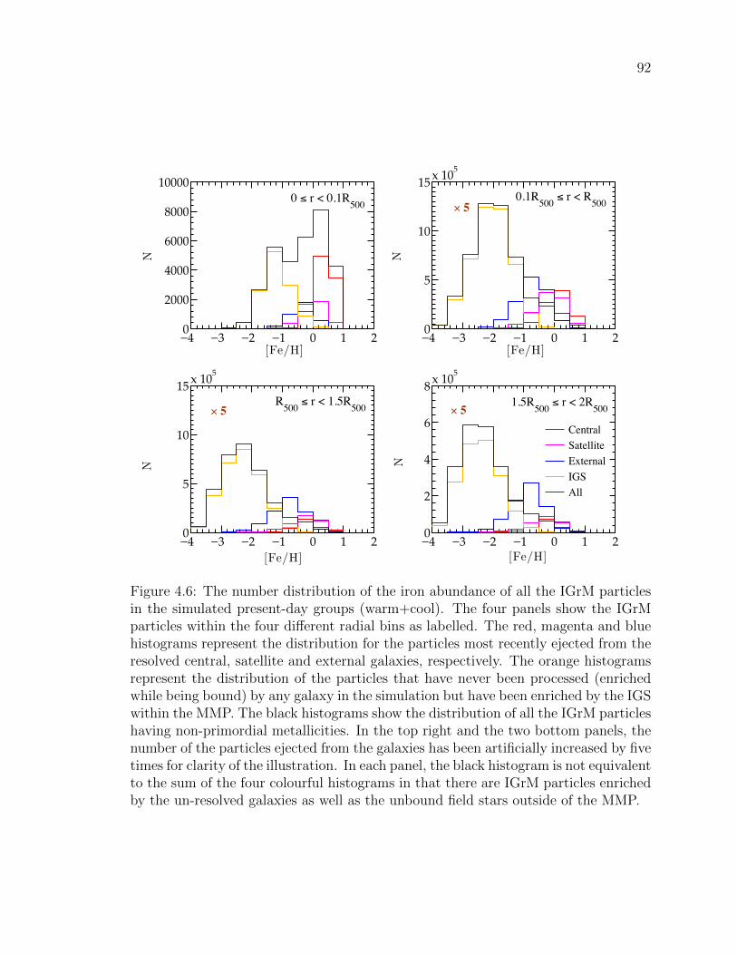
92
−4 −3 −2 −1 0 1 20
2000
4000
6000
8000
10000
[Fe/H]
N
−4 −3 −2 −1 0 1 20
5
10
15 x 105
[Fe/H]
N
−4 −3 −2 −1 0 1 20
5
10
15 x 105
[Fe/H]
N
−4 −3 −2 −1 0 1 20
2
4
6
8 x 10⁵
[Fe/H]
N
Central Satellite External IGS All
× 5
0 ) r < 0.1R500 × 50.1R500 ) r < R500
R500 ) r < 1.5R500 × 5 1.5R500 ) r < 2R500
Figure 4.6: The number distribution of the iron abundance of all the IGrM particlesin the simulated present-day groups (warm+cool). The four panels show the IGrMparticles within the four different radial bins as labelled. The red, magenta and bluehistograms represent the distribution for the particles most recently ejected from theresolved central, satellite and external galaxies, respectively. The orange histogramsrepresent the distribution of the particles that have never been processed (enrichedwhile being bound) by any galaxy in the simulation but have been enriched by the IGSwithin the MMP. The black histograms show the distribution of all the IGrM particleshaving non-primordial metallicities. In the top right and the two bottom panels, thenumber of the particles ejected from the galaxies has been artificially increased by fivetimes for clarity of the illustration. In each panel, the black histogram is not equivalentto the sum of the four colourful histograms in that there are IGrM particles enrichedby the un-resolved galaxies as well as the unbound field stars outside of the MMP.

93
from them are expected to be relatively more (less) enriched, given that the abun-
dances of the winds, in our simulation, are essentially the same as those of the ISM
of the parent galaxies from which the winds were ejected. Apart from the metal-rich
galaxy-processed particles, there are a significantly larger number of particles identi-
fied to have been enriched by the IGS in the MMP and they have significantly lower
abundances than the galaxy-processed particles. They account for the majority of
the IGrM mass within R200 (∼ 1.5R500), as is shown in the last two rows of pie charts
in Figure 4.5.
Comparing the four different panels in Figure 4.6, it is interesting to see that for
the same class of particles, there is a trend of decreasing median abundance with
increasing r(z = 0). For the “Central” category, the median gas abundance is ∼ 2
solar within 0.1R500 (top left panel) to ∼ 0.6 solar at 1.5R500 ≤ r < 2R500 (bottom
right panel); the “Satellite” category, from ∼ 1 to ∼ 0.65 solar; the “External”
category, from ∼ 0.6 to ∼ 0.15 solar; and for the “IGS” category, from ∼ 0.05
to < 0.01 solar. The trend of the “IGS” category is simply because of the higher
concentration of the diffuse IGS toward the group center compared with the IGrM
mass in the groups, which indicates that an IGrM particle at smaller r(z = 0) has
a higher chance of being enriched by the neighbouring IGS. For the three galaxy-
associated categories, intuitively, the observed trend could be a signature of the gas
at larger radius having been processed by smaller galaxies in the past, given the mass-
metallicity relation. Apart from that, this could also indicate that the gas there was
processed by much earlier galaxies, knowing that the ISM in the later galaxies has
more chance of being recycled by earlier galaxies in the past and therefore becomes
more enriched. Where and when the processed IGrM was enriched by and ejected
from the galaxies are the focus of the following subsection.
4.2.2 Where and when was the gas enriched/ejected?
After examining the sources of the metals in the present-day IGrM and their fractional
contribution, we now turn to elucidate when and where the metals were injected from
the stars. For those that were flushed out of the galaxies through the winds, we
are curious about when and where they were flushed out, and how they have been
transported to their present-day location. Answering these questions provides insights
into the evolution of the abundance profiles of the IGrM in the groups.
Following the approach of Crain et al. (2013) (also see Wiersma et al. 2010 and

94
Shen et al. 2012), we define the “enrichment radius” and the “ejection radius” as
RFe =Σi∆mi,FeriΣi∆mi,Fe
. (4.1)
For the “enrichment radius”, i in the above equation sums over all enrichment events,
∆mi,Fe is the iron increment per event, and ri is the radial distance (in physical
coordinate instead of comoving) of the enriched particle to the centre of the group
(or its MMP) at the time of enrichment. A single IGrM particle can be counted for
multiple times if it is identified to be associated to several enrichment event. For
the “ejection radius”, i instead sums over all the ejected particles, ∆mi,Fe represents
the iron mass in that particle at the time of ejection, and ri is the particle’s radial
distance at the time of ejection. In this case, an ejected particle is counted only for
once. The group center is defined as the position of the most gravitationally bound
dark matter particle within the group.
Likewise, we also make a quantitative diagnosis elucidating when the present-day
IGrM was enriched and when the metals were ejected into the IGrM from the galaxies
by defining the “enrichment redshift” and the “ejection redshift”, respectively, as
ZFe =Σi∆mi,FeziΣi∆mi,Fe
, (4.2)
where zi is the redshift at which an enrichment event/ejection occurs.
It is perhaps necessary to clarify at this point that the time and place at which
the gas is enriched is not equivalent to when and where the injected metals are
synthesized. First of all, for the low mass stars, the lag between when metals are
produced — which occurs deep in the stars — and the time when the metals are
released by stellar winds can be as long as a few Gyrs. Moreover, it is known that
there is significant gas recycling by star formation, such that the mass loss from the
old stars can be the fuel of the new generations of stars, and the metals injected
from a star particle in the simulation could have been synthesized at much earlier
epochs and in difference environments. Our simulation, like many others, does not
take record of when and where the metals are synthesized within the stars.
In Figure 4.7, we show RFe (top row) and zFe (second row) for the iron in the
present-day IGrM, against the present-day radial distance to the group center, r/Rvir(z =
0). In the left and right panels, the quantities are defined based on the conditions
of the particles at the time of enrichment and ejection, respectively. We show the
results for the overall iron (back curves) in the IGrM as well as the binned results for
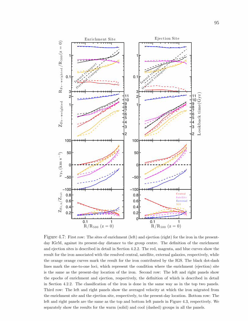
95
0.1
1
Inwa
rdt ransport
Outwa
rdt ransport
RFe−weig
hted/R
500(z
=0) Enrichment Site
0.1
1
Inwa
rdt ransport
Outwa
rdt ransport
Eject ion Site
1
23
ZFe−weighte
d
2
34567891011
1
23
2
34567891011
Lookback
time(Gyr)
0.1 1−100
−50
0
50
100
R/R500 (z = 0)
vFe(k
ms−
1 )
Central Satellite External IGS Total0.1 1
−100
−50
0
50
100
0.1 1
0.20.40.60.8
R/R500 (z = 0)
ZFe,x/Ztot
0.1 10
0.20.40.60.8
R/R500 (z = 0)
Ex te rnal
C entral
S ate l l i te
IGS
Figure 4.7: First row: The sites of enrichment (left) and ejection (right) for the iron in the present-
day IGrM, against its present-day distance to the group centre. The definition of the enrichment
and ejection sites is described in detail in Section 4.2.2. The red, magenta, and blue curves show the
result for the iron associated with the resolved central, satellite, external galaxies, respectively, while
the orange orange curves mark the result for the iron contributed by the IGS. The black dot-dash
lines mark the one-to-one loci, which represent the condition where the enrichment (ejection) site
is the same as the present-day location of the iron. Second row: The left and right panels show
the epochs of enrichment and ejection, respectively, the definition of which is described in detail
in Section 4.2.2. The classification of the iron is done in the same way as in the top two panels.
Third row: The left and right panels show the averaged velocity at which the iron migrated from
the enrichment site and the ejection site, respectively, to the present-day location. Bottom row: The
left and right panels are the same as the top and bottom left panels in Figure 4.3, respectively. We
separately show the results for the warm (solid) and cool (dashed) groups in all the panels.
96
the enrichment categories introduced in Section 4.2.1. The results for the warm and
cool groups are exhibited by the solid and dashed curves, respectively. The dashed
diagnostic black line in the top two panels marks the RFe = r(z = 0) locus, denoting
the situation where the gas is enriched/ejected at the same place as where it locates
at present day. The area below the locus indicates that the gas is enriched/ejected at
some smaller radii and then transported outwards to its current location, while the
area above represents inward motion. And finally, we note that only the results for
iron are presented because those for the other two elements are quantitatively similar
and provide no additional valuable insights.
Focusing on the top left panel, it can be seen that the iron synthesized by the
central galaxies (red) was, as expected, synthesized close to the group centre and
later transported outwards to larger distances. The “Satellite” category (magenta),
on the contrary, shows mild correlation between RFe and r(z = 0). Its curves intersect
with the one-to-one locus at r ≈ 0.6R500, indicating that the iron at r <∼ 0.6R500 in
the z = 0 groups has been transported, on the average, inwards whereas the iron at
the larger distances was transported outwards. The “External” category (blue), by
definition, represents the enrichment occurring within the galaxies outside the group
or its MMP and it is therefore not surprising to see that its curves lie beyond 2R500
(≈ Rvir). Finally, the “IGS” category (orange) shows a mild positive correlation
between RFe and r(z = 0), with RFe increasing from ∼ 0.16R500(z = 0) in the core
regions to ∼ 0.4R500(z = 0) on the outskirts and the curves intersecting with the
one-to-one locus at r ≈ 0.2R500(z = 0). The enrichment occurred at fairly inner
regions, as it is where stripping by the tidal interactions and mergers is most efficient
in the groups. The overall trend (black) is that the iron in the present-day IGrM
within 0.8R500 is, on the average, characterized by inwards motion while that at
larger distances is by outwards motion.
Turning to the top right panel, it is interesting to see that RFe defined based on
the ejection conditions is essentially the same as that for the enrichment conditions
(top left panel) for each individual category. However, for the overall iron in the IGrM
(black curves), the ejection sites are, on the average, closer to the group center. This
is because the weighting by different categories is different. As we have discussed
in the previously, a larger (smaller) amount of metals were ejected from the central
(external) galaxies into the IGrM via outflows than were actually released by the stars
within the same class of galaxies. This can also be straightforwardly seen from the
bottom panels of Figure 4.7 (the same as the left panels in Figure 4.3).

97
The second row of panels reveal that the enrichment of the IGrM proceeds, in
general, in a “outside-in” fashion, such that the metals in the more diffuse IGrM at
larger radial distances in the present-day groups were released from the stars (left
panel)/ejected into the IGrM (right panel) at relatively earlier redshifts.
Focusing first on the left panel, it can be seen that the metals at r <∼ 0.1R500 in
the z = 0 groups were on average injected from the stars to the gas phase in the
last 6 Gyrs, and those at R500 were released over 9 Gyrs ago. The same “outside-in”
fashion has previously been pointed out by Wiersma et al. (2010), in the enrichment
of the intergalactic medium, and Crain et al. (2013), in that of the circum-galactic
medium, and our result seems to show that this trend continues on the group-scale.
It also suggests that the IGrM within R500 of the present-day groups is enriched
after the groups form, i.e., when the groups assemble half of their present-day mass,
which happens about 8 − 9 Gyrs ago (c.f., Figure 13 of Chapter 3). Turning to the
individual categories, it can be seen that each of them follows the same “outside-in”
trend as the overall iron mass. The gas enriched within the external galaxies (blue)
were, as expected, enriched at the earliest epochs among all categories — 10 Gyrs
ago for metals at all radii. It can be seen that the metals synthesized within the
central (red) and satellite (magenta) galaxies are younger than the average, whereas
those produced by the external galaxies (blue) are, as expected, synthesized at much
earlier epochs — over 10 Gyrs ago for metals at all radii. For the “Central” category
(red), this “outside-in” trend is a clear signature of outward transport of metals,
insomuch as the metals at further distance would have spent longer period of time to
get transported to their present-day location. For the “Satellite” category (magenta),
we observe the same but milder correlation between ZFe and r(z = 0), and compared
with the “Central” category, it appears to be chemically older. Finally, it is interesting
to see that the iron injected from the IGS was, on the average, ejected most recently
among all the categories, which is not surprising, as the delayed Type Ia SNe and
AGB stars in the field become effective source of iron only at late epochs.
Looking at the right panel, the ejection redshift vs. r(z = 0) relation of each
of the three galaxy-related categories displays similar feature as the corresponding
curve in the left panel, yet shows an offset towards the low-z direction. The offset is a
signature of the lag in ejection, that a gas particle could be processed (bound to and
enriched) within different galaxies for multiple times, which is frequently observed in
massive galaxies and at low redshifts (see Oppenheimer & Dave, 2008; Oppenheimer
et al., 2010). The ejection time shown in the right panel only records the last ejection

98
event for each ejected particle so therefore is supposed to be later than the averaged
enrichment time. In detail, the discrepancy between the two red curves is greater in
the core regions than on the groups’ outskirts, which indicates that the gas at the inner
regions, being ejected at more recent epochs, has a larger chance and longer history
of being recycled by the central galaxies. It is perhaps surprising to notice that the
two magenta curves also display quite significant discrepancy — the ejection curve in
the right panel is 0.5−1 Gyr lower. One might naively think that this is an indicator
of gas recycling within the satellite galaxies, yet we have checked and confirmed that
this could rarely happen. A fraction of the gas enriched within the satellite galaxies
was later ejected from the central galaxies after merger, and on average, that is the
part of gas that was enriched much earlier as it has gone through a longer period of
time to enter the central galaxies, be ejected, and travel to its present-day location.
In the right panel, the magenta curve does not include this early-enriched gas that
was eventually ejected from the central galaxies.
Another important problem is how fast the metals have traveled to their present-
day radius from the place where they were injected by the stars, and ejected by the
galaxies via wind. An order of magnitude calculation can be done simply by dividing
r(z = 0) − RFe by tFe (the look back time corresponding to the enrichment/ejection
redshift). In the third row of panels in Figure 4.7, we show the resulting quantity,
vFe, as a function of r(z = 0). Positive vFe in the two panels indicates outward
transport, corresponding to the area below the one-to-one locus in the top panels,
whereas negative vFe represents inwards motion, and to the area above the locus.
In general, we see that the metals in the IGrM migrate at a few 10 km s−1 within
the groups. Examining the individual categories, it is perhaps worth-noting that
the transport speed of the in-situ wind enrichment (i.e.,“Central” and “Satellite”
categories) is comparable with that of the gas enriched by the IGS. The key is that
the metals injected from the IGS are not driven by the outflows so therefore the
feature pointed out strongly indicates that the merger-induced convection, instead of
the wind ejection, is the dominant mechanism for transporting the metals to their
present-day location in the groups.
4.3 Conclusions
The main findings of this chapter are as follows.

99
(i) Our simulation produces iron abundance profiles that broadly match the obser-
vation data, except that in the innermost regions (R <∼ 0.1R500), the simulated
abundances are more concentrated, due to the overproduction of stars in the
groups’ central galaxy. The flattened shape of the ZSi/ZFe profiles out to R500
is consistent with the recent Suzaku observations.
(ii) Under the schema of the momentum-driven wind, the produced iron abundance
profiles show increasing concentration with decreasing redshift at z >∼ 1. This is
because of the wind particles ejected from the central as well as infalling galaxies
becoming confined to a smaller fraction of the virial radius of the parent halos,
ram-pressure stripping being more efficient at inner regions where density is
higher, and the re-accretion of processed, enriched gas that are ejected at higher
redshifts.
(iii) We find that from z = 3 to z = 0, the ZSi/ZFe of the hot gas within Rvir declines
by∼ 15%. Knowing that the Type II SNe dominate the silicon production based
on our cosmic chemical model (see OD08). The ZSi/ZFe of the hot gas at z = 3
is essentially the combined yields of the Type II SNe and the prompt Type Ia
SNe, we estimate from the decline of ZSi/ZFe that the delayed Type Ia SNe
contribute roughly 1/7 of the iron in the present-day IGrM. The decline of the
ZSi/ZFe of the hot halo gas extends to ∼ 4R500, beyond which the ZSi/ZFe is
essentially unchanged.
(iv) The IGrM in the present-day groups is dominated by the gas that has never
been processed (bound and enriched) by any galaxy during the assembly history
of the groups. The overall mass fraction of the galaxy-processed IGrM shows
strong gradient against radius, declining from above 50% at r ≤ 0.1R500 to
∼ 5% at r = 2R500(≈ Rvir). The warm groups have a higher fraction of the
IGrM processed by the galaxies than the cool groups, accounting for the higher
abundance profiles.
(v) The metals found in the IGrM can be synthesized by the stars within the central,
satellite galaxies of the groups’ most massive progenitors (MMP), the external
galaxies outside the MMPs, as well as by the diffuse and unbound intra-group
stars (IGS). We find that the central galaxies dominate the production of the
metals in the IGrM from the group centre to ∼ R500, and the metals in the outer
regions are more synthesized by the external galaxies. The satellite galaxies are
100
important but sub-dominant contributors to the metals at all radii in the groups.
And importantly, we find that the IGS contribute nontrivial amount of iron in
the IGrM. The IGS account for relatively lower fraction of the oxygen and
silicon mass in the z = 0 IGrM than the iron. This results from the fact that
the enrichment associated with the IGS, being old stellar populations stripped
from the galaxies, is primarily due to the metals from the delayed enrichment
from the Type Ia SNe and the AGB stars.
(vi) Finally, we find that the enrichment of the IGrM follows an outside-in fashion,
that is, the IGrM in the more inner regions is enriched at later epochs by various
resources than at larger distances. There is a trend of outward transport of the
IGrM metals over the assembly history of the groups, of which the average
speed is a few 10 km s−1. The metal transport in the IGrM is more driven by
the merger-induced gas convection inside the groups.

101
Chapter 5
SUMMARY AND FUTURE
OUTLOOK
A wealth of observational and theoretical studies have advanced galaxy groups as the
best candidates for studying the very processes associated with galaxy formation and
evolution. The hot and diffuse gaseous component that permeates the group halos, or
the intra-group medium (IGrM), is accessible to X-ray observations, and its observable
properties provide very important constraints to these processes. This dissertation
represents one such effort, where we examine the growth and chemical enrichment
of the IGrM using the cosmological simulation that includes a well-constrained pre-
scription for large-scale, momentum-driven, galactic outflows powered by stars and
supernovae, as well as a sophisticated model for cosmic chemical evolution. Our wind
and chemical models have previously been shown to be very successful at reproducing
the intergalactic medium (IGM) observations simultaneously with a range of galaxy
observables (e.g. Oppenheimer & Dave, 2009; Dave, Oppenheimer & Finlator, 2011).
Extending the study to galaxy groups, Dave, Oppenheimer & Sivanandam (2008)
found that it could also yield both the iron abundance and the oxygen-to-iron ratio
of the present-day IGrM that well match the observations. Nevertheless, the sim-
ulation produced more stars in the groups than observed, indicating that another
feedback mechanism, such as AGN feedback, should be introduced to provide further
quenching of star formation. We follow the work by DOS08, to investigate in greater
detail how the enrichment of the IGrM proceeds based on the simulation schemes,
how much the excessive star formation in the groups would affect the robustness of
the success, and hope to get better constraints to the nature of AGN feedback.

102
In the “Conclusions” sections of the two main chapters (Chapter 3 and 4), we
provide a detailed description of all our findings. Here in this Chapter, we only sum-
marize the most important of them:
• Our simulation with momentum-driven outflows is very successful at regulating
the stellar mass of the group galaxies at M∗ < 1011 M; however, we also find galaxies
— typically, one per group and invariably, the group central galaxy — that has much
larger stellar mass than any observed galaxy. The excess stellar mass of the groups
is, in contrast with expectations, not owing to catastrophic cooling of the IGrM, but
rather the build-up of cold gas in those massive galaxies before they are incorporated
into the groups. Our finding suggests that in order to reduce the stellar mass fraction
to match the observed data, the required additional feedback mechanism must be
powerful enough to expel a significant fraction of the emerging halo gas component
from the galactic halos.
• The simulated hot gas fraction of the simulated z = 0 groups is in broad agree-
ment with the observations, except perhaps that in the rich group regime, it is slightly
higher than the latter. This results in several scaling relationships, depending on the
structure and state of the IGrM, fitting fairly well with the observational results, but
for the most massive groups tending to be more luminous in X-ray than are observed.
This indicates that the stellar-powered outflows become ineffectual and a required
additional feedback mechanism is needed to effectively puff the hot IGrM to more
extended configuration in those massive systems. Comparing the groups at different
redshifts, we notice that for groups with comparable temperature (depth of potential
well), the IGrM mass fraction increases between z = 3 to z = 1, as the efficacy of
galactic winds to maintain an extended hot gas distribution via heating declines dur-
ing this period. This evolution of IGrM mass fraction has imprints upon the scaling
relationships over the same time period, the cosmic expansion-corrected X-ray lumi-
nosity increases, whereas the corrected core gas entropy declines accordingly as the
hot gas becomes more compact in the groups. At z <∼ 1, the hot gas in the groups
tends to stabilize, and so do the scaling relationships.
•We find that the simulated iron and silicon abundances of the present-day IGrM,
both emission-weighed and mass-weighted, fit fairly well with the observations. We
specifically identified the sources of metals in today’s IGrM. A rough estimation re-
veals that even after removing the metals synthesized by the excessive amount of
stars in the “over-sized” galaxies, the global abundances are still within the accept-

103
able range given the uncertainties in the metals yields and supernova rates. The
central galaxies dominates the metal production in the central regions, but its frac-
tional contribution declines as a function of distance towards the group centre. A
non-trivial amount of metals in the IGrM were synthesized within the galaxies while
they were satellites or outside of the group MMP, and they account for larger frac-
tional contribution of metals as it goes to outer regions of the groups. There’s clear
age gradient, such that metals in the inner regions were produced more recently than
those at outer regions. It should be stressed that the IGS in the groups produce
significant amount of iron to today’s IGrM, via delayed Type Ia SNe and AGB mass
loss, and it’s relative contribution increases with decreasing group mass.
It is somehow fortunate that though our simulation has failed at reproducing the
observed stellar mass fraction of galaxy groups due to lacking AGN, the produced
metal content of the IGrM is still in broad agreement with observations, primarily
because the amount of metals deposited into the IGrM does not grow linearly with star
formation of the galaxies in the groups. For those ‘over-sized” galaxies in the groups,
the mass outflow rate becomes only a fraction of the star formation rate, indicating
that the metals produced within those galaxies are more likely to be locked in stars.
Moreover, those galaxies reside in the densest regions in the simulation volume where
gravitational and viscous drag are most efficient, so that the wind particles behave
more like fountains and therefore very limited fraction of the excessive metals are
retained in the IGrM.
Certainly this thesis does not mark the end of the project, but only the first
step in a long journey towards faithfully reproducing all, or more safely speaking, as
many observables related to galaxy groups (and clusters) by state-of-art simulation
techniques. And in order to achieve so, we will continue incorporating the simulation
with new prescriptions for the missing physics. These physics may have limited,
or only second-order influence on the large-scale distribution of metals in the IGrM
(in comparison with the resolution limit of ∼5 kpc), which is the main focus of
this work, but for many other problems, can be of vital importance — e.g. star
formation in the central galaxies, core gas entropy, the observed population of cool-
core groups/clusters, the observed scatter in the scaling relationships, etc. Here we
list three main problems that currently attract most of our attention:
1. AGN feedback

104
Observational evidence of AGN interacting with the environments has been
widely seen, including high-speed winds, jet-induced bubbles, shock fronts and
ripples (McNamara & Nulsen, 2007; Fabian, 2012, and references therein). Yet
the implementation of AGN feedback in cosmological simulations turns out to
be a non-trivial task, given that the accretion of gas onto the blackholes and the
coupling of feedback energy with the environments involve a variety of physical
processes that operate on spatial scales spanning across many orders of magni-
tude. To model all these processes simultaneously is far beyond the capability
of the current cosmological simulations and moreover, many details of these
processes are still theoretically and observationally ill-constrained. At present,
there is a wide variance in the sub-resolution recipes adopted in different cos-
mological simulations, lying in five major aspects — 1) how the mass accretion
rate onto the blackhole is calculated given the limited resolution; 2) how indi-
vidual gas particles are “absorbed” by the blackhole in the simulations; 3) how
much of the accreted rest mass is returned as feedback energy and the way in
which it is returned (i.e. by thermalizing nearby SPH particles or by increasing
their momentum); 4) the blackhole advection algorithm (to avoid the blackholes
from being inappropriately dragged around by two-body forces); and 5) black-
hole merger algorithm — as summarized by Wurster & Thacker (2013). These
different recipes often introduce a number of free parameters that are calibrated
in an ad hoc fashion to fit the variety of observational results, such as the black-
hole growth, the correlations between blackholes and host galaxies, the comic
star formation history, and the hot gas and baryonic faction within halos (e.g.
Power, Nayakshin & King, 2011; Dubois et al., 2012; Rosas-Guevara et al., 2013;
Vogelsberger et al., 2013; Angles-Alcazar et al., 2015; Crain et al., 2015). A de-
tailed physical understanding of the ad hoc parameterization remains lacking,
and is where much progress can be made.
2. Turbulent mixing
As a “classical” particle-based, Lagrangian method, SPH does not include any
implicit diffusion of scalar quantities such as metals, leading to artificial inho-
mogeneities in metal distribution (Wiersma et al., 2009). In nature, however,
turbulence is prevalent and is expected to cause mixing of metals between gases.
For instance, the ISM is known to be highly turbulent, owing to SN explosions,
thermal and gravitational instability (Elmegreen & Scalo, 2004; Mac Low &

105
Klessen, 2004; Yang & Krumholz, 2012; Petit et al., 2015). Turbulence is also
expected to be prevalent in ICM/IGrM given the high Reynold number associ-
ated with its violent dynamical motions (Fujita, Takizawa & Sarazin, 2003). As
for the IGM, the strongest recent evidence of turbulence is from the study of
low-z OVI absorption (Oppenheimer & Dave, 2009; Oppenheimer et al., 2012).
One would also anticipate that the large shear velocity between the outflowing
material in the winds and the ambient halo gas is likely to drive turbulence
via Kelvin-Helmholtz instability, leading to metal mixing. There are recent
attempts to impose sub-grid recipes for turbulent diffusion into the hierarchi-
cal galaxy formation models (e.g. Greif et al., 2009; Shen, Wadsley & Stinson,
2010), but it still remains unclear how efficiently metals can mix on different
scales and in different environments, since the related physical processes are
still poorly understood. And moreover, we are also particularly interested in
how turbulent mixing promotes heat transfer in the IGrM/ICM, the interplay
between turbulence, magnetic field and cosmic rays, and how this interplay may
impact the mixing properties of the IGrM/ICM. There are several important
observational projects taking place, or on the horizon, that may advance our
knowledge of the detailed gas dynamics in various environments, and out to
high redshifts (e.g. Astro-H, ALMA, SKA) (see Somerville & Dave, 2014, for
reviews).
3. Magnetohydrodynamic instabilities
The IGrM/ICM is comprised of weakly collisional magnetized plasma where the
Coulomb mean free path of the elementary particles is many orders of magni-
tude larger than their gyroradius, and the conductive flow of heat is strongly
anisotropic with respect to the local magnetic field direction since the thermal
collisions across the field lines are largely restricted. The anisotropic conduction
in the IGrM/ICM is expected to drive two kinds of convection instabilities: the
magnetothermal instability, or MTI (Balbus, 2000; Parrish, Stone & Lemaster,
2008), occurring when temperature increases in the direction of gravity and
the heat-flux-driven-buoyancy instability, or HBI (Parrish & Quataert, 2008;
Quataert, 2008), with inverted temperature profiles. It has been found that the
MTI and HBI instabilities could have profound impact on the thermal conduc-
tion in the IGrM/ICM by altering the local topology of the magnetic field. We
are interested in its implications for the observed bi-modality of groups/clusters

106
and the non-thermal pressure support in the IGrM/ICM (Parrish, Quataert &
Sharma, 2009, 2010; Parrish et al., 2012).
To summarize, while this simulation has produced thermal and chemical properties
of the IGrM in reasonably good agreement with the observations, there is still much
work to be done to get many other observable properties of galaxy groups/clusters
correct. Adding new improvements to the code could be extremely exhilarating yet
challenging, as it requires advancement in observational and numerical techniques,
as well as deeper understanding of the core physical processes involved. We are
ready to welcome the forthcoming new twists, shocking surprises, and unexpected
new discoveries.

107
Bibliography
Abadi M. G., Moore B., Bower R. G., 1999, MNRAS, 308, 947
Alpaslan M. et al., 2012, MNRAS, 426, 2832
Anders E., Grevesse N., 1989, Geochim. Cosmochim. Acta, 53, 197
Angles-Alcazar D., Dave R., Ozel F., Oppenheimer B. D., 2014, ApJ, 782, 84
Angles-Alcazar D., Ozel F., Dave R., Katz N., Kollmeier J. A., Oppenheimer B. D.,
2015, ApJ, 800, 127
Arth A., Dolag K., Beck A. M., Petkova M., Lesch H., 2014, ArXiv e-prints
Babul A., Balogh M. L., Lewis G. F., Poole G. B., 2002, MNRAS, 330, 329
Babul A., Sharma P., Reynolds C. S., 2013, ApJ, 768, 11
Bahe Y. M., McCarthy I. G., Balogh M. L., Font A. S., 2013, MNRAS, 430, 3017
Balbus S. A., 2000, ApJ, 534, 420
Balogh M. L., Babul A., Patton D. R., 1999, MNRAS, 307, 463
Balogh M. L., Mazzotta P., Bower R. G., Eke V., Bourdin H., Lu T., Theuns T.,
2011, MNRAS, 412, 947
Balogh M. L., Morris S. L., 2000, MNRAS, 318, 703
Barnes J. E., 1988, ApJ, 331, 699
Bildfell C., Hoekstra H., Babul A., Mahdavi A., 2008, MNRAS, 389, 1637
Binney J., Tremaine S., 1987, Galactic dynamics

108
Birkinshaw M., 1999, Phys. Rep., 310, 97
Bırzan L., Rafferty D. A., McNamara B. R., Wise M. W., Nulsen P. E. J., 2004, ApJ,
607, 800
Bosch B. et al., 2013, A&A, 549, A142
Bournaud F., Elmegreen B. G., Teyssier R., Block D. L., Puerari I., 2010, MNRAS,
409, 1088
Bradshaw E. J. et al., 2013, MNRAS, 433, 194
Brook C. B. et al., 2011, MNRAS, 415, 1051
Carlstrom J. E., Holder G. P., Reese E. D., 2002, ARA&A, 40, 643
Carroll S. M., Press W. H., Turner E. L., 1992, ARA&A, 30, 499
Catinella B. et al., 2013, MNRAS, 436, 34
Cavagnolo K. W., Donahue M., Voit G. M., Sun M., 2008, ApJ, 683, L107
Chabrier G., 2003, PASP, 115, 763
Chandrasekhar S., 1942, Principles of stellar dynamics
Connelly J. L. et al., 2012, ApJ, 756, 139
Crain R. A., Eke V. R., Frenk C. S., Jenkins A., McCarthy I. G., Navarro J. F.,
Pearce F. R., 2007, MNRAS, 377, 41
Crain R. A., McCarthy I. G., Schaye J., Theuns T., Frenk C. S., 2013, MNRAS, 432,
3005
Crain R. A. et al., 2015, MNRAS, 450, 1937
Dalla Vecchia C., Schaye J., 2008, MNRAS, 387, 1431
Dalla Vecchia C., Schaye J., 2012, MNRAS, 426, 140
Dave R., 2009, in Astronomical Society of the Pacific Conference Series, Vol. 419,
Galaxy Evolution: Emerging Insights and Future Challenges, Jogee S., Marinova
I., Hao L., Blanc G. A., eds., p. 347

109
Dave R. et al., 2001, ApJ, 552, 473
Dave R., Finlator K., Oppenheimer B. D., 2006, MNRAS, 370, 273
Dave R., Finlator K., Oppenheimer B. D., 2011a, MNRAS, 416, 1354
Dave R., Finlator K., Oppenheimer B. D., 2011b, MNRAS, 416, 1354
Dave R., Oppenheimer B. D., Finlator K., 2011, MNRAS, 415, 11
Dave R., Oppenheimer B. D., Sivanandam S., 2008, MNRAS, 391, 110
De Grandi S., Ettori S., Longhetti M., Molendi S., 2004, A&A, 419, 7
De Grandi S., Molendi S., 2002, ApJ, 567, 163
de Plaa J., Werner N., Bleeker J. A. M., Vink J., Kaastra J. S., Mendez M., 2007,
A&A, 465, 345
Diaferio A., 1999, MNRAS, 309, 610
Diaferio A., Geller M. J., 1997, ApJ, 481, 633
D’Odorico V., Cupani G., Cristiani S., Maiolino R., Molaro P., Nonino M., Centurion
M., Cimatti, 2013, MNRAS, 435, 1198
Domainko W. et al., 2006, A&A, 452, 795
Dressler A., 1980, ApJ, 236, 351
Dubois Y., Devriendt J., Slyz A., Teyssier R., 2012, MNRAS, 420, 2662
Dubois Y., Teyssier R., 2008, A&A, 477, 79
Eckmiller H. J., Hudson D. S., Reiprich T. H., 2011, A&A, 535, A105
Edge A. C., Stewart G. C., 1991, MNRAS, 252, 414
Edge A. C., Stewart G. C., Fabian A. C., 1992, MNRAS, 258, 177
Egami E. et al., 2006, ApJ, 647, 922
Eisenstein D. J., Hu W., 1999, ApJ, 511, 5
Elmegreen B. G., Scalo J., 2004, ARA&A, 42, 211

110
Ettori S., 2015, MNRAS, 446, 2629
Ettori S., Fabian A. C., 1999, MNRAS, 305, 834
Evans, II N. J. et al., 2009, ApJS, 181, 321
Evrard A. E., Henry J. P., 1991, ApJ, 383, 95
Fabian A. C., 1994, ARA&A, 32, 277
Fabian A. C., 2012, ARA&A, 50, 455
Fabian A. C., Hu E. M., Cowie L. L., Grindlay J., 1981, ApJ, 248, 47
Fabian A. C., Nulsen P. E. J., Canizares C. R., 1984, Nature, 310, 733
Fabjan D., Borgani S., Tornatore L., Saro A., Murante G., Dolag K., 2010, MNRAS,
401, 1670
Faucher-Giguere C.-A., Quataert E., 2012, MNRAS, 425, 605
Federrath C., Klessen R. S., 2013, ApJ, 763, 51
Finlator K., Dave R., 2008, MNRAS, 385, 2181
Finlator K., Dave R., Papovich C., Hernquist L., 2006, ApJ, 639, 672
Finlator K., Oppenheimer B. D., Dave R., 2011, MNRAS, 410, 1703
Finoguenov A., Ponman T. J., Osmond J. P. F., Zimer M., 2007, MNRAS, 374, 737
Ford A. B., Dave R., Oppenheimer B. D., Katz N., Kollmeier J. A., Thompson R.,
Weinberg D. H., 2014, MNRAS, 444, 1260
Fujita Y., Ohira Y., 2012, ApJ, 746, 53
Fujita Y., Ohira Y., 2013, MNRAS, 428, 599
Fujita Y., Takizawa M., Sarazin C. L., 2003, ApJ, 584, 190
Fukazawa Y., Makishima K., Tamura T., Ezawa H., Xu H., Ikebe Y., Kikuchi K.,
Ohashi T., 1998, PASJ, 50, 187
Gabor J. M., Bournaud F., 2014, MNRAS, 441, 1615
111
Gabor J. M., Dave R., 2012, MNRAS, 427, 1816
Gabor J. M., Dave R., 2015, MNRAS, 447, 374
Geach J. E. et al., 2014, Nature, 516, 68
Giodini S. et al., 2012, A&A, 538, A104
Giodini S., Lovisari L., Pointecouteau E., Ettori S., Reiprich T. H., Hoekstra H.,
2013, Space Sci. Rev., 177, 247
Giodini S., Pierini D., Finoguenov A. e., 2009, ApJ, 703, 982
Gonzalez A. H., Sivanandam S., Zabludoff A. I., Zaritsky D., 2013, ApJ, 778, 14
Governato F., Willman B., Mayer L., Brooks A., Stinson G., Valenzuela O., Wadsley
J., Quinn T., 2007, MNRAS, 374, 1479
Greif T. H., Glover S. C. O., Bromm V., Klessen R. S., 2009, MNRAS, 392, 1381
Gunn J. E., Gott, III J. R., 1972, ApJ, 176, 1
Haines C. P. et al., 2015, ArXiv e-prints
Haines C. P. et al., 2013, ApJ, 775, 126
Hellwing W. A., Li B., Frenk C. S., Cole S., 2013, MNRAS, 435, 2806
Helsdon S. F., Ponman T. J., 2000, MNRAS, 315, 356
Helsdon S. F., Ponman T. J., 2003, MNRAS, 339, L29
Hinshaw G. et al., 2013, ApJS, 208, 19
Hirschmann M. et al., 2013, MNRAS, 436, 2929
Hoekstra H., Bartelmann M., Dahle H., Israel H., Limousin M., Meneghetti M., 2013,
Space Sci. Rev., 177, 75
Hopkins P. F., Keres D., Onorbe J., Faucher-Giguere C.-A., Quataert E., Murray N.,
Bullock J. S., 2014, MNRAS, 445, 581
Hopkins P. F., Quataert E., Murray N., 2012, MNRAS, 421, 3522
112
Hoyle B., Masters K. L., Nichol R. C., Jimenez R., Bamford S. P., 2012, MNRAS,
423, 3478
Hummels C. B., Bryan G. L., 2012, ApJ, 749, 140
Just A., Khan F. M., Berczik P., Ernst A., Spurzem R., 2011, MNRAS, 411, 653
Kaiser N., 1986, MNRAS, 222, 323
Kaiser N., 1991, ApJ, 383, 104
Katz N., Weinberg D. H., Hernquist L., 1996, ApJS, 105, 19
Kennicutt, Jr. R. C., 1998, ApJ, 498, 541
Keres D., Katz N., Dave R., Fardal M., Weinberg D. H., 2009, MNRAS, 396, 2332
Keres D., Katz N., Weinberg D. H., Dave R., 2005, MNRAS, 363, 2
Kettula K. et al., 2013, ApJ, 778, 74
Knobel C. et al., 2009, ApJ, 697, 1842
Komarov S. V., Churazov E. M., Schekochihin A. A., ZuHone J. A., 2014, MNRAS,
440, 1153
Kravtsov A. V., Nagai D., Vikhlinin A. A., 2005, ApJ, 625, 588
Krumholz M. R., Dekel A., McKee C. F., 2012, ApJ, 745, 69
Krumholz M. R., Thompson T. A., 2013, MNRAS, 434, 2329
Kunz M. W., 2011, MNRAS, 417, 602
Kunz M. W., Bogdanovic T., Reynolds C. S., Stone J. M., 2012, ApJ, 754, 122
Lagana T. F., de Souza R. S., Keller G. R., 2010, A&A, 510, A76
Lagana T. F., Martinet N., Durret F., Lima Neto G. B., Maughan B., Zhang Y.-Y.,
2013, A&A, 555, A66
Larson R. B., Tinsley B. M., Caldwell C. N., 1980, ApJ, 237, 692
Leauthaud A. et al., 2010, ApJ, 709, 97

113
Leauthaud A. et al., 2012, ApJ, 746, 95
Lewis G. F., Babul A., Katz N., Quinn T., Hernquist L., Weinberg D. H., 2000, ApJ,
536, 623
Limongi M., Chieffi A., 2005, in Astronomical Society of the Pacific Conference Series,
Vol. 342, 1604-2004: Supernovae as Cosmological Lighthouses, Turatto M., Benetti
S., Zampieri L., Shea W., eds., p. 122
Lin Y.-T., Mohr J. J., Stanford S. A., 2003, ApJ, 591, 749
Lokas E. L., Hoffman Y., 2001, in Identification of Dark Matter, Spooner N. J. C.,
Kudryavtsev V., eds., p. 121
Mac Low M.-M., Klessen R. S., 2004, Reviews of Modern Physics, 76, 125
Mahdavi A., Hoekstra H., Babul A., Bildfell C., Jeltema T., Henry J. P., 2013, ApJ,
767, 116
Mahdavi A., Hoekstra H., Babul A., Henry J. P., 2008, MNRAS, 384, 1567
Markevitch M., 1998, ApJ, 504, 27
Markevitch M., Forman W. R., Sarazin C. L., Vikhlinin A., 1998, ApJ, 503, 77
Martin C. L., 2005, ApJ, 621, 227
Martin C. L., 2006, ApJ, 647, 222
Maughan B. J., Giles P. A., Randall S. W., Jones C., Forman W. R., 2012, MNRAS,
421, 1583
Mazzotta P., Rasia E., Moscardini L., Tormen G., 2004, MNRAS, 354, 10
McCarthy I. G., Babul A., Bower R. G., Balogh M. L., 2008, MNRAS, 386, 1309
McCarthy I. G., Balogh M. L., Babul A., Poole G. B., Horner D. J., 2004, ApJ, 613,
811
McCarthy I. G., Le Brun A. M. C., Schaye J., Holder G. P., 2014, MNRAS, 440, 3645
McCarthy I. G., Schaye J., Bower R. G., Ponman T. J., Booth C. M., Dalla Vecchia
C., Springel V., 2011, MNRAS, 412, 1965

114
McCarthy I. G. et al., 2010, MNRAS, 406, 822
McCourt M., Quataert E., Parrish I. J., 2013, MNRAS, 432, 404
McDonald M. et al., 2013, ApJ, 774, 23
McNamara B. R., Nulsen P. E. J., 2007, ARA&A, 45, 117
McNamara B. R. et al., 2014, ApJ, 785, 44
Mo H., van den Bosch F. C., White S., 2010, Galaxy Formation and Evolution
Moore B., Katz N., Lake G., Dressler A., Oemler A., 1996, Nature, 379, 613
Muratov A. L., Keres D., Faucher-Giguere C.-A., Hopkins P. F., Quataert E., Murray
N., 2015, ArXiv e-prints
Murray N., Menard B., Thompson T. A., 2011, ApJ, 735, 66
Murray N., Quataert E., Thompson T. A., 2005, ApJ, 618, 569
Nagai D., 2006, ApJ, 650, 538
Nagai D., Kravtsov A. V., Vikhlinin A., 2007, ApJ, 668, 1
Nagai D., Vikhlinin A., Kravtsov A. V., 2007, ApJ, 655, 98
Nagashima M., Lacey C. G., Baugh C. M., Frenk C. S., Cole S., 2005, MNRAS, 358,
1247
Nipoti C., Treu T., Ciotti L., Stiavelli M., 2004, MNRAS, 355, 1119
Oppenheimer B. D., Dave R., 2006, MNRAS, 373, 1265
Oppenheimer B. D., Dave R., 2008, MNRAS, 387, 577
Oppenheimer B. D., Dave R., 2009, MNRAS, 395, 1875
Oppenheimer B. D., Dave R., Finlator K., 2009, MNRAS, 396, 729
Oppenheimer B. D., Dave R., Katz N., Kollmeier J. A., Weinberg D. H., 2012, MN-
RAS, 420, 829

115
Oppenheimer B. D., Dave R., Keres D., Fardal M., Katz N., Kollmeier J. A., Weinberg
D. H., 2010, MNRAS, 406, 2325
Osmond J. P. F., Ponman T. J., 2004, MNRAS, 350, 1511
Ostriker J. P., Hausman M. A., 1977, ApJ, 217, L125
Ostriker J. P., Tremaine S. D., 1975, ApJ, 202, L113
O’Sullivan E. et al., 2012, MNRAS, 424, 2971
O’Sullivan E., Kolokythas K., Raychaudhury S., Vrtilek J. M., Kantharia N., 2014,
ArXiv e-prints
Parrish I. J., McCourt M., Quataert E., Sharma P., 2012, MNRAS, 422, 704
Parrish I. J., Quataert E., 2008, ApJ, 677, L9
Parrish I. J., Quataert E., Sharma P., 2009, ApJ, 703, 96
Parrish I. J., Quataert E., Sharma P., 2010, ApJ, 712, L194
Parrish I. J., Stone J. M., Lemaster N., 2008, ApJ, 688, 905
Peterson J. R., Kahn S. M., Paerels F. B. S., Kaastra J. S., Tamura T., Bleeker
J. A. M., Ferrigno C., Jernigan J. G., 2003, ApJ, 590, 207
Petit A. C., Krumholz M. R., Goldbaum N. J., Forbes J. C., 2015, MNRAS, 449,
2588
Piontek F., Steinmetz M., 2011, MNRAS, 410, 2625
Pipino A., Kaviraj S., Bildfell C., Babul A., Hoekstra H., Silk J., 2009, MNRAS, 395,
462
Planelles S., Borgani S., Fabjan D., Killedar M., Murante G., Granato G. L., Ragone-
Figueroa C., Dolag K., 2014, MNRAS, 438, 195
Pope E. C. D., 2010, MNRAS, 404, 451
Pope E. C. D., Babul A., Pavlovski G., Bower R. G., Dotter A., 2010, MNRAS, 406,
2023

116
Postman M., Geller M. J., 1984, ApJ, 281, 95
Pounds K. A., King A. R., Page K. L., O’Brien P. T., 2003a, MNRAS, 346, 1025
Pounds K. A., Reeves J. N., King A. R., Page K. L., O’Brien P. T., Turner M. J. L.,
2003b, MNRAS, 345, 705
Power C., Nayakshin S., King A., 2011, MNRAS, 412, 269
Pratt G. W. et al., 2010, A&A, 511, A85
Pratt G. W., Croston J. H., Arnaud M., Bohringer H., 2009, A&A, 498, 361
Puchwein E., Sijacki D., Springel V., 2008, ApJ, 687, L53
Quataert E., 2008, ApJ, 673, 758
Rasia E. et al., 2012, New Journal of Physics, 14, 055018
Rasmussen J., Ponman T. J., 2007, MNRAS, 380, 1554
Rasmussen J., Ponman T. J., 2009, MNRAS, 399, 239
Revaz Y., Combes F., Salome P., 2008, A&A, 477, L33
Robotham A. S. G. et al., 2011, MNRAS, 416, 2640
Rosas-Guevara Y. M. et al., 2013, ArXiv e-prints
Rosati P., Borgani S., Norman C., 2002, ARA&A, 40, 539
Rupke D. S., Veilleux S., Sanders D. B., 2005, ApJS, 160, 115
Russell H. R. et al., 2014, ApJ, 784, 78
Saintonge A. et al., 2011, MNRAS, 415, 32
Sales L. V., Navarro J. F., Schaye J., Dalla Vecchia C., Springel V., Booth C. M.,
2010, MNRAS, 409, 1541
Sanderson A. J. R., O’Sullivan E., Ponman T. J., 2009, MNRAS, 395, 764
Sasaki T., Matsushita K., Sato K., 2014, ApJ, 781, 36
117
Sato K., Kawaharada M., Nakazawa K., Matsushita K., Ishisaki Y., Yamasaki N. Y.,
Ohashi T., 2010, PASJ, 62, 1445
Scannapieco E., Bildsten L., 2005, ApJ, 629, L85
Schaye J. et al., 2015, MNRAS, 446, 521
Schmidt F., Lima M., Oyaizu H., Hu W., 2009, Phys. Rev. D, 79, 083518
Sell P. H. et al., 2014, MNRAS, 441, 3417
Shen S., Madau P., Aguirre A., Guedes J., Mayer L., Wadsley J., 2012, ApJ, 760, 50
Shen S., Wadsley J., Stinson G., 2010, MNRAS, 407, 1581
Simionescu A., 2009, PhD thesis, Ludwig-Maximilians-Universitat Munchen
Sivanandam S., Zabludoff A. I., Zaritsky D., Gonzalez A. H., Kelson D. D., 2009,
ApJ, 691, 1787
Smith R. K., Brickhouse N. S., Liedahl D. A., Raymond J. C., 2001, ApJ, 556, L91
Soko lowska A., Mayer L., Babul A., Madau P., Shen S., 2015, ArXiv e-prints
Somerville R. S., Dave R., 2014, ArXiv e-prints
Springel V., 2005, MNRAS, 364, 1105
Springel V., Hernquist L., 2003, MNRAS, 339, 289
Stinson G. S., Brook C., Maccio A. V., Wadsley J., Quinn T. R., Couchman H. M. P.,
2013, MNRAS, 428, 129
Sturm E. et al., 2011, ApJ, 733, L16
Sun M., 2012, New Journal of Physics, 14, 045004
Sun M., Voit G. M., Donahue M., Jones C., Forman W., Vikhlinin A., 2009, ApJ,
693, 1142
Taranu D. S., Hudson M. J., Balogh M. L., Smith R. J., Power C., Oman K. A.,
Krane B., 2014, MNRAS, 440, 1934
Teyssier R., Chapon D., Bournaud F., 2010, ApJ, 720, L149

118
Thompson T. A., Fabian A. C., Quataert E., Murray N., 2015, MNRAS, 449, 147
Tombesi F., Cappi M., Reeves J. N., Palumbo G. G. C., Yaqoob T., Braito V., Dadina
M., 2010a, A&A, 521, A57
Tombesi F., Sambruna R. M., Reeves J. N., Braito V., Ballo L., Gofford J., Cappi
M., Mushotzky R. F., 2010b, ApJ, 719, 700
Toomre A., Toomre J., 1972, ApJ, 178, 623
Tozzi P., Norman C., 2001, ApJ, 546, 63
Turner M. L., Schaye J., Steidel C. C., Rudie G. C., Strom A. L., 2014, MNRAS,
445, 794
van den Bosch F. C., Aquino D., Yang X., Mo H. J., Pasquali A., McIntosh D. H.,
Weinmann S. M., Kang X., 2008, MNRAS, 387, 79
van der Burg R. F. J., Muzzin A., Hoekstra H., Wilson G., Lidman C., Yee H. K. C.,
2014, A&A, 561, A79
Vanderlinde K. et al., 2010, ApJ, 722, 1180
Veilleux S. et al., 2013, ApJ, 776, 27
Vikhlinin A., Kravtsov A., Forman W., Jones C., Markevitch M., Murray S. S., Van
Speybroeck L., 2006, ApJ, 640, 691
Vikhlinin A. et al., 2009, ApJ, 692, 1060
Villar Martın M., Emonts B., Humphrey A., Cabrera Lavers A., Binette L., 2014,
MNRAS, 440, 3202
Vogelsberger M., Genel S., Sijacki D., Torrey P., Springel V., Hernquist L., 2013,
MNRAS, 436, 3031
Voit G. M., Bryan G. L., 2001, Nature, 414, 425
White S. D. M., Efstathiou G., Frenk C. S., 1993, MNRAS, 262, 1023
Wiersma R. P. C., Schaye J., Dalla Vecchia C., Booth C. M., Theuns T., Aguirre A.,
2010, MNRAS, 409, 132

119
Wiersma R. P. C., Schaye J., Theuns T., Dalla Vecchia C., Tornatore L., 2009,
MNRAS, 399, 574
Williams C. C. et al., 2014, ApJ
Wurster J., Thacker R. J., 2013, MNRAS, 431, 2513
Yang C.-C., Krumholz M., 2012, ApJ, 758, 48
Zel’dovich Y. B., 1970, A&A, 5, 84
Zeldovich Y. B., 1972, MNRAS, 160, 1P
Zhu G., Zheng Z., Lin W. P., Jing Y. P., Kang X., Gao L., 2006, ApJ, 639, L5