The Greenness of Rural and Urban Pakistan Over Time ...

The Greenness of Rural and Urban Pakistan Over Time:

Household Energy Use and Carbon Emissions

Syed M. Hasan

Assistant Professor, Department of Economics

Lahore University of Management Sciences

D.H.A, Lahore Cantt. 54792

Lahore, Pakistan

Email: [email protected]

Phone: +92-331-5036704

Wendong Zhang

Assistant Professor, Department of Economics

Iowa State University

478C Heady Hall, 518 Farmhouse Lane, Ames, Iowa 50011

Email: [email protected]

Phone: 515-294-2536 / Fax: 515-294-0221

Acknowledgement

The authors would like to thank the participants of Sustainability and Development Conference

(SDC), 2018 for their valuable comments and suggestions. Hasan acknowledges and appreciates

the excellent research assistance provided by Mr. Attique ur Rehman and the departmental

funding provided by the department of Economics, LUMS, Lahore.

mailto:[email protected]

mailto:[email protected]



Abstract:

This study provides the first empirical estimates of household energy use and carbon emissions

from 2005 to 2014 for all Pakistani rural and urban districts, using four rounds of nationwide

household survey data. This is significant, because Pakistan is the sixth most populous country in

the world and has the highest population growth rate and urbanization level of all South Asian

countries. Following Glaeser and Kahn (2010), we estimate and predict carbon emissions every 2

years during 2005-2014 for each district in Pakistan using household-level survey data on energy

consumption. We then rank all districts based on the predicted carbon emissions for

representative median households, rating districts with less per capita carbon emissions as

greener, and finally explain the changes in the district’s “greenness” rank over time. We find,

first, that Pakistan’s capital, Islamabad, has the higher per capita emissions, at 1 ton per year in

2013-14, and emission hotspots tend to cluster around urban centers and remote rural areas with

heavy reliance on firewood use. Although Pakistan’s major cities’ household carbon emissions

are still drastically lower than in the U.S., they are comparable to, and sometimes even higher

than, cities in India and China. Second, our results demonstrate the importance of accounting for

carbon emissions over time using multiple rounds of surveys—as opposed to focusing on a

single year—because 52% of Pakistani districts experienced changes in their greenness rankings

over the past decade. Finally, we show that while electricity, gasoline, and natural gas

consumption drive carbon emissions in urban districts in Pakistan, firewood accounts for half of

all carbon emissions in rural areas in KP and Balochistan provinces. Ignoring household garbage,

therefore, would lead to underestimation of the urban carbon footprint by at least 15% in

developing countries such as Pakistan.

1



1. Introduction

Urbanization is arguably the most consequential phenomenon impacting billions of people across

the globe. The United Nations estimates that the share of the world’s population that lives in

cities will double from 30% in 1950 to 60% in 2030 (UN 2014). In addition, urbanization,

especially in the developing world, has occurred at an unprecedented pace over the past few

decades. However, the positive spillovers of cities—the agglomeration economies—do not come

without a cost: Around the globe, many cities face significant challenges in the provision of

public services as well as diverse environmental impacts, which include the carbon footprint. For

example, cities account for about 43% of global primary energy-related carbon dioxide

emissions (Seto et al. 2014). More importantly, there is a lack of systematic understanding of the

ecological and environmental footprint of growing cities, especially for cities and peri-urban

areas in developing countries that are experiencing the greatest wave of urbanization in human

history. Arguably, many growing cities in developing countries are on unsustainable trajectories,

and are thus likely have disproportionately larger environmental impacts—such as air pollution

and greenhouse gas emissions—relative to the size of their population or economy (Rees 2006).

This issue is often exacerbated for developing countries, which often lack adequate and cost-

efficient abatement technologies and an environmentally friendly regulatory environment,

especially in cities or neighborhoods with higher concentrations of poorer households.

The relationship between energy use, urban growth, and carbon emissions has been

extensively analyzed, but many previous studies focus on aggregate or sectoral direct energy use

(e.g., Zhang 2000; Hertwich and Peters 2009; Han and Chatterjee 1997; Levitt et al. 2017) or

2

aggregate land use change (e.g., Naughton-Treves 2004). Recently, efforts have been made to

understand urban households’ carbon emissions for cities in the U.S. (Glaeser and Kahn 2010);

China (Zheng et al. 2011); U.K. (Minx et al. 2013); Philippines (Serino and Klasen 2015); and

India (Ahmad et al. 2015) using household-level data. This paper is the first such study for

Pakistan, which is the sixth most populous country in the world and has the highest population

and urbanization growth rate of all South Asian countries (Kedir et al. 2016). The United Nations

estimates that half of Pakistan’s population will live in urban areas by 2030, which means that

roughly 60 million people will move from rural areas to cities over the next decade (UN 2014).

More importantly, all of the aforementioned studies use cross-sectional data collected at a single

point in time, which only provides a snapshot of the carbon footprint of cities for that particular

time and ignores the dynamic linkages between climate footprint and rapid urbanization,

migration, and income growth, as well as technological improvements in carbon abatement

technologies.

In addition, most previous studies only examine urban households and largely ignore

rural and peri-urban areas; this is problematic, especially for developing countries experiencing

rapid urbanization. Finally, all previous studies ignore two important sources of carbon

emissions: firewood use and household garbage. On the one hand, firewood is still used by over

2 billion people across the globe and is sometimes the only domestically available and affordable

source of energy, especially for low-income developing countries (FAO 2017). On the other

hand, food loss and waste and other household garbage are garnering growing global recognition

as a critical problem in both developed and developing countries (Lipinski et al. 2013). Our

paper improves on previous literature on all three fronts by employing multiple years of

3

household surveys, expanding the sample to both rural and urban households, and incorporating

firewood use and household garbage in our analysis.

The primary objective of this paper is to quantify, for the first time, a district’s carbon

emissions based on a representative household’s energy consumption for both urban and rural

districts in Pakistan and the district’s changes over time. Unlike previous studies that rely on a

single snapshot of cross-sectional surveys, we use the four most recent rounds of micro-level

data from the Pakistan Social and Living Standards Measurement (PSLM) Survey. The survey

represents the most comprehensive nationwide dataset at the household level in Pakistan in terms

of household demographic and socioeconomic characteristics and, in particular, disaggregated

energy consumption expenditures at the household level. Specifically, we use the 2005-06, 2007-

08, 2010-11, and 2013-14 PSLM surveys. Following Glaeser and Kahn (2010), and for each

round of the survey from 2005 to 2014, we predict the carbon emissions for 77 major rural and

urban districts in Pakistan based on energy consumption by a provincially representative

household, then rank all districts based on their “greenness,” which is implied by the predicted

aggregate carbon emissions at the district level.

To do so, we first estimate a series of Heckman selection models of household energy

consumption to predict the consumption of each energy type by standardized households at the

provincial level, then translate these predicted energy consumption values into carbon dioxide

emissions using well-established emission conversion factors from the Intergovernmental Panel

on Climate Change (IPCC) Emission Factors Database (EFDB) (IPCC 2017). Relying on survey

weights, we also obtain the weighted sum of carbon emissions by district, energy type, and year.

Therefore, we effectively create a district-level panel dataset of carbon emissions by energy type,

which not only allows us to obtain a ranking of districts’ greenness, based on their per capita

4

carbon emissions for each survey year, but also offers opportunities to examine cross-district

differences in the trajectories of energy use and carbon emissions from 2005 to 2014.

Our main findings reveal the significance and importance of panel data over time in

understanding the dynamic linkages between urban development, energy use, and carbon

footprint: 52% of Pakistani districts experienced changes in their greenness rankings over the

past decade. In particular, 18% of Pakistani districts became significantly greener when

measured by per capita emissions from 2005 to 2014, while 34% became less green. Our results

also show that the hotspots for carbon emissions in Pakistan tend to cluster around megacities;

Islamabad has the highest per capita carbon emissions, at 1 ton per year. Although Pakistan’s

major cities’ household carbon emissions are still drastically lower than in the U.S., they are

comparable to, and sometimes even higher than, cities in India and China. In addition, districts of

different sizes exhibit different trajectories in their per capita household emissions from 2005 to

2014: Rural districts’ household emissions decline because of a greater supply of electricity and

reduced use of firewood, while households in megacities with at least 1 million residents

experience a U-shaped change in carbon emissions. We also find that the composition of energy

types that contribute to carbon emissions varies significantly in urban and rural districts.

Specifically, while electricity, gasoline, and natural gas consumption drive carbon emissions in

urban districts in Pakistan, firewood accounts for half of all carbon emissions in rural areas in KP

and Balochistan provinces. Finally, our results show that ignoring household garbage would lead

to underestimation of the urban carbon footprint by at least 10%.

Our paper makes several important contributions to the understanding of linkages between

urban growth and climate change, energy consumption and carbon emissions, carbon accounting,

and sustainable development. First, using a unique set of micro-level household survey data for

5

every 2 years for both urban and rural areas in Pakistan since 2004, this paper provides the first

empirical analysis of how Pakistani households’ energy use and carbon emissions change over

time amid rapid urbanization and population growth and how rural and urban districts evolve

from 2005 to 2014 in their greenness, as measured by per capita and total carbon emissions. This

is particularly important because Pakistan—and developing countries in general—experienced

much faster population growth over the past few decades, coupled with unprecedented

urbanization. Second, rather than relying on a single year’s data, as in previous studies, we use

four rounds of household surveys spanning over a decade, and thus are able to identify the

different trajectories of carbon emissions for each district. Our main results demonstrate the

drawbacks of relying on one year’s data, due to rapid changes in the districts’ urban development

trajectories. Third, our analysis not only includes information on urban households, but also

covers rural and emerging urban districts, both of which are vitally important in developing

countries that face urbanization pressures. Finally, we show that firewood use and household

garbage are critical in determining household carbon emissions; ignoring them, as most previous

studies do, would lead to gross underestimation of the carbon footprint in developing countries

such as Pakistan.

2. Background

As the sixth most populous country in the world and the most rapidly urbanizing South Asian

nation (Kugelman 2015), Pakistan offers an excellent laboratory for examining the dynamic

linkages between urban growth and carbon emissions. According to the most recent population

census conducted in 2017, Pakistan’s population grows at 2.4% annually, which is the fastest of

all countries in South Asia. Data from the World Bank’s World Development Indicators (WDI)

6

show that the population of Pakistani cities grows at an even faster pace: 2.6% annually (World

Bank, 2016). The WDI database also shows that Pakistan is comparable to lower-middle-income

(LMC) countries in terms of urban population growth and carbon emissions; Pakistan’s carbon

dioxide intensity relative to GDP is 0.88 kg/dollars for LMC countries on average, and 0.83 for

Pakistan.

Sustainable development and the impacts of climate change are growing concerns for both

developed and developing countries, and especially for urbanizing countries such as Pakistan.

The IPCC (2014) finds that globally, 32% of the rural population lacks access to electricity and

other modern energy sources, compared to only 5.3% of the urban population (IEA, 2010).

Hence, energy use and the consequent greenhouse gas (GHG) emissions from human settlements

are mainly from urban areas, and therefore the role of cities and urban areas in global climate

change has become increasingly important over time (Seto et al. 2014). A World Bank (2010)

study states that economic growth and urbanization have moved in a cyclical manner, similar to

the observed trend of economic growth and GHG emissions, for at least the last 100 years. With

Pakistan experiencing rapid population growth, especially in cities, we can expect Pakistan to

contribute more GHG emissions globally, surpassing its current 1% of the world’s total (IPCC

2017). This will require better understanding of the impacts of urbanization, energy use, and

climate change for both urban and emerging urban areas.

The Global Climate Risk Index developed by Germanwatch (Kreft et al. 2015) ranks

Pakistan among the top 10 countries most affected by climate change during the last 20 years—

and the adverse impacts of climate change are getting more serious with time: Pakistan rose from

10th place in 1994-2013 to 8th place in 1995-2014. Salam (2018) reports that Pakistan’s 200

million residents are among the world's most vulnerable to the growing consequences of climate

7

change. During this period, Pakistan has also suffered from increasingly frequent climate-

induced catastrophes. For instance, unusual heatwaves have occurred in Karachi, the largest city,

over the last few years; in 2015, about 1,200 people lost their lives due to an unprecedented heat

wave in the city, which was partly caused by the urban heat island (UHI) effect (Sajjad et al.

2015). The UHI effect is not uniform across the city, and instead has the highest impact in areas

in which greenery is scarce and the density of human activity is high. Similarly, the Washington

Post reported that in 2018, a city in the Sindh province of Pakistan recorded the hottest

temperature ever observed on the planet in the month of April. Also in 2018, Malik Amin Aslam,

Pakistan’s Advisor to the Prime Minister on Climate Change, stated that in the last 20 years,

Pakistan has suffered a loss of Rs14 billion due to climate change and is the second largest

country to suffer such a big loss due to the issue (Pakistan Today, 2018). As a result, Pakistan is

not only expected to emit more carbon dioxide; it is also a major victim of ongoing climate

change, especially in rural areas in which proper abatement technologies are frequently not

available.

In developing countries such as Pakistan, millions of residents also face the challenge of

limited energy supply due to poor planning and lack of investment. According to International

Energy Agency (2016) statistics, at least 51 million people in Pakistan—27% of the

population—do not have access to electricity. In its annual State of the Industry Report, the

Pakistan National Electric Power Regulatory Authority (NEPRA) reported in 2016 that

approximately 20% of all villages—32,889 out of 161,969—are not connected to the grid

(NEPRA, 2016). Even those households that have connections experience daily blackouts; it is

estimated that more than 144 million people across the country do not have reliable access to

electricity (World Bank, 2017), which varies from more than 90% of households in urban areas

8

to only 61% in remote rural areas (Agency, 2017). As a result, Pakistan’s energy mix and

technologies are more complex than those of the developed countries previous studies focus on:

More than 50% of the population, mainly in rural Pakistan, relies on traditional biomass for

cooking. Common cooking fuels include firewood, agricultural waste, and dung cakes. This

takes a heavy toll, with more than 50,000 premature deaths due to indoor air pollution—

especially exposure to smoke and soot from cooking—every year in Pakistan (Sanchez-Triana,

2015). The issue is also further exacerbated by poor planning, which largely ignores the demands

of rural households and forces many rural households to use firewood and other biomass fuels

(Kugelman 2015). This suggests that biomass fuels such as firewood will play a much more

significant role in understanding household energy use and carbon emissions in developing

countries such as Pakistan—a factor that is largely nonexistent in developed countries.

3. Data and Methodology

We aim to quantify the household- and district-level carbon emissions for almost all districts in

Pakistan over the past decade. To do that, we follow a five-step approach in which we (1)

explain household-level energy consumption using household demographic and socioeconomic

characteristics based on several nationwide household surveys; (2) predict district-level energy

consumption for all districts using the characteristics of provincially representative households;

(3) convert predicted energy consumption to carbon emissions for all districts using well-

established carbon emission factors; (4) rank districts’ greenness based on predicted carbon

emissions; and (5) identify the determinants of changes in districts’ greenness rankings over time

using district-level panel data estimation. We will discuss these methods in more detail below, as

well as the data used to implement these estimations.

9

Step 0. Data preparation and validation

We first link multiple nationwide datasets for the first time to obtain a complete picture of energy

consumption by Pakistani households for all energy types. The first dataset is the Pakistan Social

and Living Standards Measurement (PSLM) Survey, a restricted-access, nationally

representative survey that provides household-level energy consumption and income data. The

PSLM surveys used here were conducted in alternate years at the provincial and district levels

from July 2004 to June 2015, and cover almost all urban areas in Pakistan and roughly 40% of

all households in cities. Specifically, we use household-level data for 64,760 households from

the PSLM survey conducted in the financial years 2005-06, 2007-08, 2011-12, and 2013-14.

Survey data collection is based on stratified sampling of both urban and rural areas. Of particular

interest to our study, PSLM data have disaggregated household-level expenditures for various

fuel and energy types, including cooking fuel, lighting fuel, and electricity. To convert these

energy expenditures to energy consumption in quantity, we use the annual national energy prices

provided by the Pakistan Economic Survey from 2005 to 2014 (Pakistan Economic Survey 2014).

In particular, we obtain energy and fuel consumption quantities for electricity, natural gas,

gasoline, CNG, LPG, and firewood.

Unfortunately the PSLM survey does not cover public transportation usage for all

households from 2005 to 2014. As a result, we rely on the newly added section on household

expenditure on public transport in the 2015-2016 round of the PSLM survey. We first use 2015-

2016 average expenditures across three household types—high, medium, and low—for all

districts on four modes of public transportation: cab, bus, rickshaw, and minivan. With this

expenditure, we construct and calculate the share of total household energy expenditure on for

public transportation for 2015-2016, then back out energy expenditure on public transportation

10

from 2005 to 2014 by maintaining the same ratio. Finally, energy expenditure on public transport

was converted to consumption quantities using average national prices from the Pakistan

Economic Survey in corresponding years.

A unique addition to our study is the carbon emissions generated by household garbage.

To obtain this, we use Pakistani government data that separately report average garbage quantity

generated by households in urban and rural regions for each of the four provinces in Pakistan.

Using these per capita per day figures, we estimate the amount of garbage generated by each

household included in the analysis. However, we only include garbage quantity for households

that have no formal system of garbage collection, because in such cases open burning is the usual

method of disposal.

Table 1 shows the summary statistics for household demographic and socioeconomic

characteristics form the PSLM survey. On average, 60% of the households are in rural areas,

with 24% of households consisting of agricultural producers and workers. The average

household size is close to seven, which is much larger than the norm in the developed world. Of

particular significance to our study, Table 1 shows that almost no households rely on coal for

heating or cooking, although this is likely to change with more coal-based power plants as part of

the China Pakistan Economic Corridors. On average, 35% of households have connections to

electricity, 35% have natural gas connections, 18% live in a municipality that collects household

garbage, and only 5% own a private car.

Step 1. Explaining household-level energy consumption

To understand and explain the determinants of household-level energy consumption, we follow

Gleaser and Kahn (2010) and run a series of Heckman selection models using the household

11

Table 1: Summary Statistics of Household Characteristics and Energy Consumption

VARIABLES N mean sd Min max

Annual Income (PKR,

1USD~100PKR) 64,760 172,221 334,538 0 5.134e+07

Household Size 64,761 6.850 3.406 1 61

Age (years) 64,681 45.90 13.63 10 99

Married 64,761 0.902 0.29 0 1

Employer 52,908 0.018 0.133 0 1

Self-Employed 52,908 0.187 0.390 0 1

Paid Employee 52,908 0.553 0.497 0 1

Agri Worker 52,908 0.236 0.425 0 1

Educated 62,821 0.903 0.295 0 1

Household with Electricity

Connection 64,761 0.349 0.476 0 1

Annual Electricity (KWh) 57,564 1,723 1,625 0 74,213

Household with Gas Connection 64761 0.346 0.475 0 1

Annual Natural Gas (MMBTU) 24,564 48.84 32.19 0 681.8

Car Ownership (Yes/No) 64,761 0.0510 0.220 0 1

District Gasoline(for Cab liters) 57,486 5.651 9.189 0 163.4

District HSD(for Bus liters) 57,486 21.60 20.06 0.0974 270.6

District LPG(for Rickshaw kgs) 57,486 1.419 1.237 0 17.08

District CNG(for Minivan kgs) 57,486 3.742 9.234 0 151.9

District Garbage Generation 57,486 887.3 514.7 102.2 9,817

District Coal Use 64,761 0.00411 0.0640 0 1

Waste Collection by Municipality 64,757 0.184 0.387 0 1

Rural 64,761 0.605 0.488 0 1

Elevation (meters) 63897 412.1019 615.5532 9 3377

12

surveys for each energy type (Heckman 1976). It is important to account for sample selection

issues, because not all energy types are available to all households in Pakistan. Instead, our

survey shows that only 35% of Pakistani households have access to electricity or natural gas, and

only 5% of households own motor vehicles. The PSLM surveys not only have information on

energy expenditure, but also on asset ownership, such as motor vehicles, and access to energy,

such as connections to electricity or a natural gas supply. This provides several natural exclusion

restrictions for constructing two-stage Heckman selection models using these asset ownership

and energy access variables as exclusion restrictions.

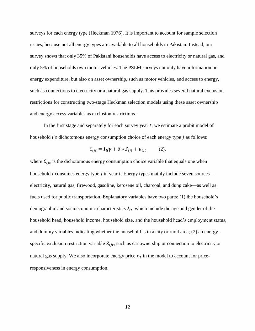
In the first stage and separately for each survey year 𝑡, we estimate a probit model of

household 𝑖′𝑠 dichotomous energy consumption choice of each energy type 𝑗 as follows:

𝐶𝑖𝑗𝑡 = 𝑰𝒊𝒕𝜸 + 𝛿 ∗ 𝑍𝑖𝑗𝑡 + 𝑢𝑖𝑗𝑡 (2),

where 𝐶𝑖𝑗𝑡 is the dichotomous energy consumption choice variable that equals one when

household 𝑖 consumes energy type 𝑗 in year 𝑡. Energy types mainly include seven sources—

electricity, natural gas, firewood, gasoline, kerosene oil, charcoal, and dung cake—as well as

fuels used for public transportation. Explanatory variables have two parts: (1) the household’s

demographic and socioeconomic characteristics 𝑰𝒊𝒕, which include the age and gender of the

household head, household income, household size, and the household head’s employment status,

and dummy variables indicating whether the household is in a city or rural area; (2) an energy-

specific exclusion restriction variable 𝑍𝑖𝑗𝑡, such as car ownership or connection to electricity or

natural gas supply. We also incorporate energy price 𝑟𝑗𝑡 in the model to account for price-

responsiveness in energy consumption.

13

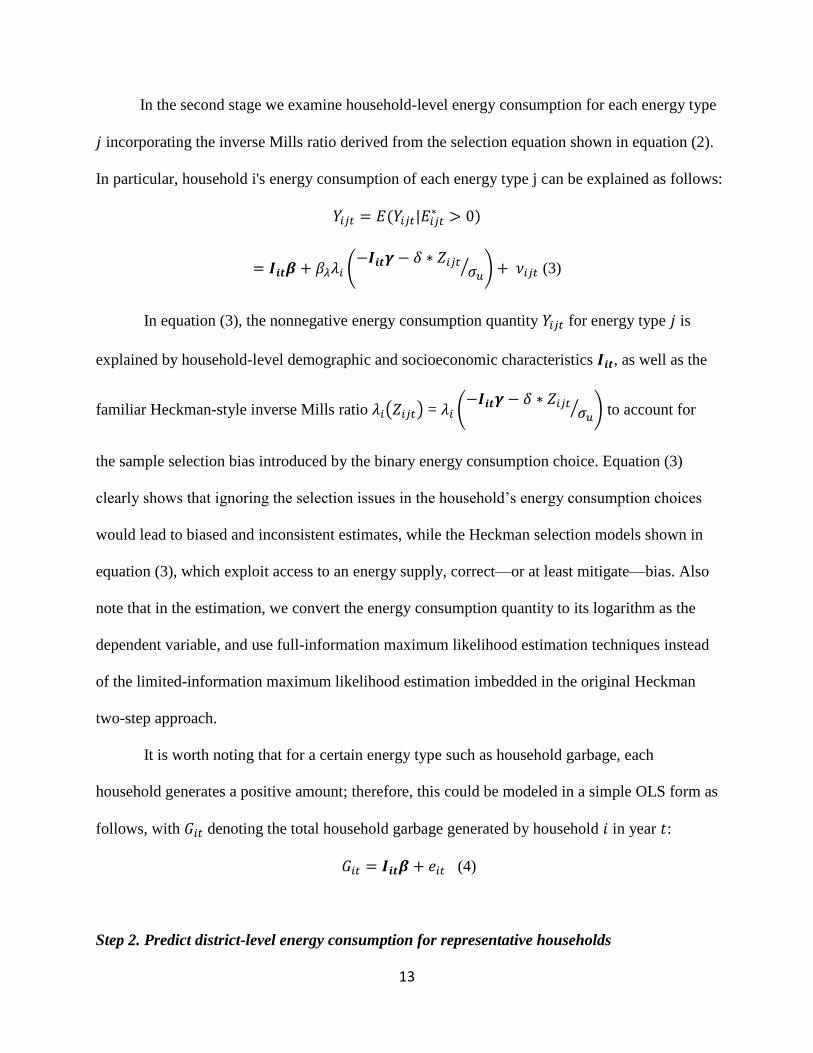
In the second stage we examine household-level energy consumption for each energy type

𝑗 incorporating the inverse Mills ratio derived from the selection equation shown in equation (2).

In particular, household i's energy consumption of each energy type j can be explained as follows:

𝑌𝑖𝑗𝑡 = 𝐸(𝑌𝑖𝑗𝑡|𝐸𝑖𝑗𝑡∗ > 0)

= 𝑰𝒊𝒕𝜷 + 𝛽𝜆𝜆𝑖 (−𝑰𝒊𝒕𝜸 − 𝛿 ∗ 𝑍𝑖𝑗𝑡

𝜎𝑢⁄ ) + 𝜈𝑖𝑗𝑡 (3)

In equation (3), the nonnegative energy consumption quantity 𝑌𝑖𝑗𝑡 for energy type 𝑗 is

explained by household-level demographic and socioeconomic characteristics 𝑰𝒊𝒕, as well as the

familiar Heckman-style inverse Mills ratio 𝜆𝑖(𝑍𝑖𝑗𝑡) = 𝜆𝑖 (−𝑰𝒊𝒕𝜸 − 𝛿 ∗ 𝑍𝑖𝑗𝑡

𝜎𝑢⁄ ) to account for

the sample selection bias introduced by the binary energy consumption choice. Equation (3)

clearly shows that ignoring the selection issues in the household’s energy consumption choices

would lead to biased and inconsistent estimates, while the Heckman selection models shown in

equation (3), which exploit access to an energy supply, correct—or at least mitigate—bias. Also

note that in the estimation, we convert the energy consumption quantity to its logarithm as the

dependent variable, and use full-information maximum likelihood estimation techniques instead

of the limited-information maximum likelihood estimation imbedded in the original Heckman

two-step approach.

It is worth noting that for a certain energy type such as household garbage, each

household generates a positive amount; therefore, this could be modeled in a simple OLS form as

follows, with 𝐺𝑖𝑡 denoting the total household garbage generated by household 𝑖 in year 𝑡:

𝐺𝑖𝑡 = 𝑰𝒊𝒕𝜷 + 𝑒𝑖𝑡 (4)

Step 2. Predict district-level energy consumption for representative households

14

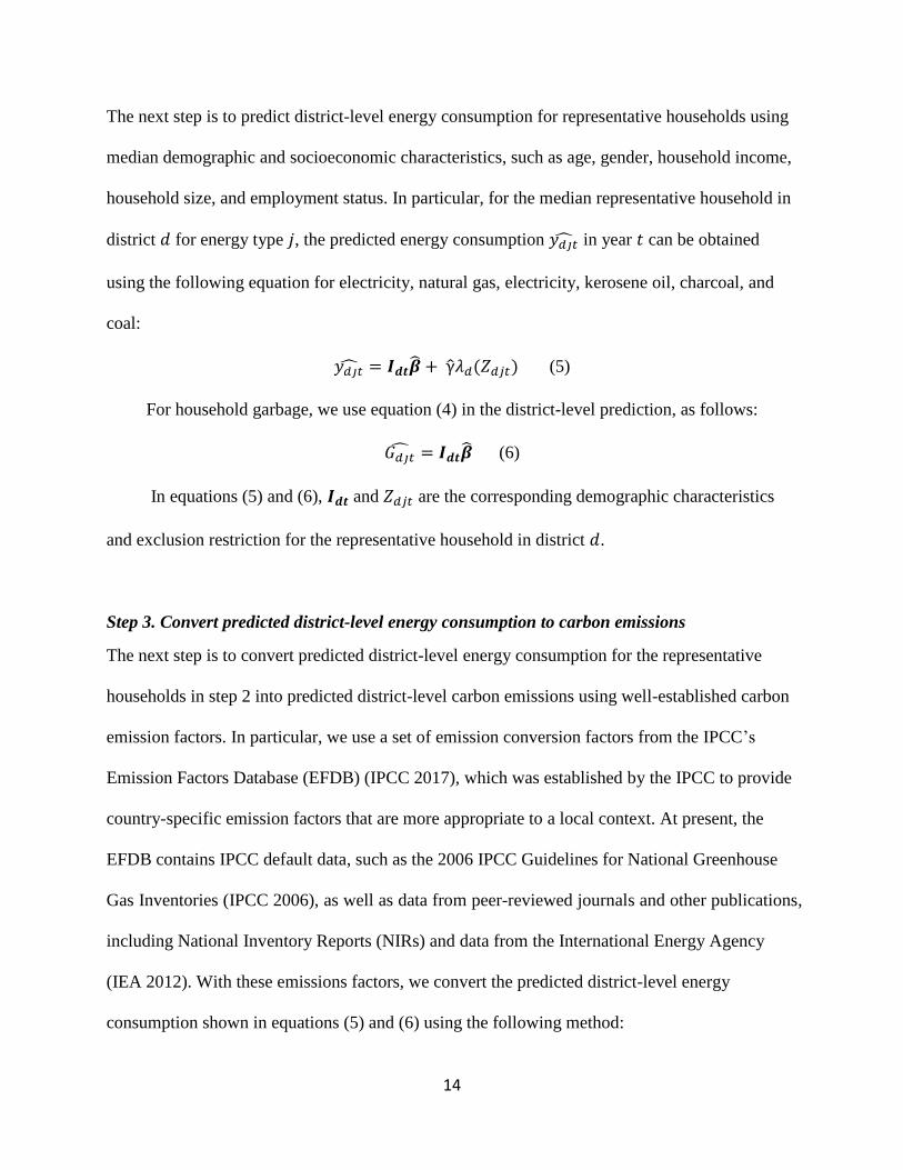
The next step is to predict district-level energy consumption for representative households using

median demographic and socioeconomic characteristics, such as age, gender, household income,

household size, and employment status. In particular, for the median representative household in

district 𝑑 for energy type 𝑗, the predicted energy consumption 𝑦𝑑𝑗𝑡 in year 𝑡 can be obtained

using the following equation for electricity, natural gas, electricity, kerosene oil, charcoal, and

coal:

𝑦𝑑𝑗𝑡 = 𝑰𝒅𝒕�� + γ𝜆𝑑(𝑍𝑑𝑗𝑡) (5)

For household garbage, we use equation (4) in the district-level prediction, as follows:

𝐺𝑑𝑗𝑡 = 𝑰𝒅𝒕�� (6)

In equations (5) and (6), 𝑰𝒅𝒕 and 𝑍𝑑𝑗𝑡 are the corresponding demographic characteristics

and exclusion restriction for the representative household in district 𝑑.

Step 3. Convert predicted district-level energy consumption to carbon emissions

The next step is to convert predicted district-level energy consumption for the representative

households in step 2 into predicted district-level carbon emissions using well-established carbon

emission factors. In particular, we use a set of emission conversion factors from the IPCC’s

Emission Factors Database (EFDB) (IPCC 2017), which was established by the IPCC to provide

country-specific emission factors that are more appropriate to a local context. At present, the

EFDB contains IPCC default data, such as the 2006 IPCC Guidelines for National Greenhouse

Gas Inventories (IPCC 2006), as well as data from peer-reviewed journals and other publications,

including National Inventory Reports (NIRs) and data from the International Energy Agency

(IEA 2012). With these emissions factors, we convert the predicted district-level energy

consumption shown in equations (5) and (6) using the following method:

15

𝐸𝑑𝑗𝑡 = 𝑦𝑑𝑗𝑡 ∗ 𝐸𝐹𝑗 (7a)

𝐸𝑑𝐺�� = 𝐺𝑑�� ∗ 𝐸𝐹𝐺 (7b)

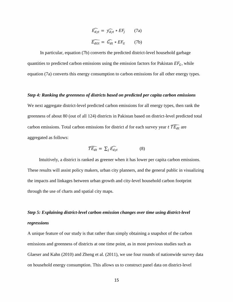
In particular, equation (7b) converts the predicted district-level household garbage

quantities to predicted carbon emissions using the emission factors for Pakistan 𝐸𝐹𝐺 , while

equation (7a) converts this energy consumption to carbon emissions for all other energy types.

Step 4: Ranking the greenness of districts based on predicted per capita carbon emissions

We next aggregate district-level predicted carbon emissions for all energy types, then rank the

greenness of about 80 (out of all 124) districts in Pakistan based on district-level predicted total

carbon emissions. Total carbon emissions for district 𝑑 for each survey year 𝑡 𝑇𝐸𝑑�� are

aggregated as follows:

𝑇𝐸𝑑�� = ∑ 𝐸𝑑𝑗𝑡

𝑗 (8)

Intuitively, a district is ranked as greener when it has lower per capita carbon emissions.

These results will assist policy makers, urban city planners, and the general public in visualizing

the impacts and linkages between urban growth and city-level household carbon footprint

through the use of charts and spatial city maps.

Step 5: Explaining district-level carbon emission changes over time using district-level

regressions

A unique feature of our study is that rather than simply obtaining a snapshot of the carbon

emissions and greenness of districts at one time point, as in most previous studies such as

Glaeser and Kahn (2010) and Zheng et al. (2011), we use four rounds of nationwide survey data

on household energy consumption. This allows us to construct panel data on district-level

16

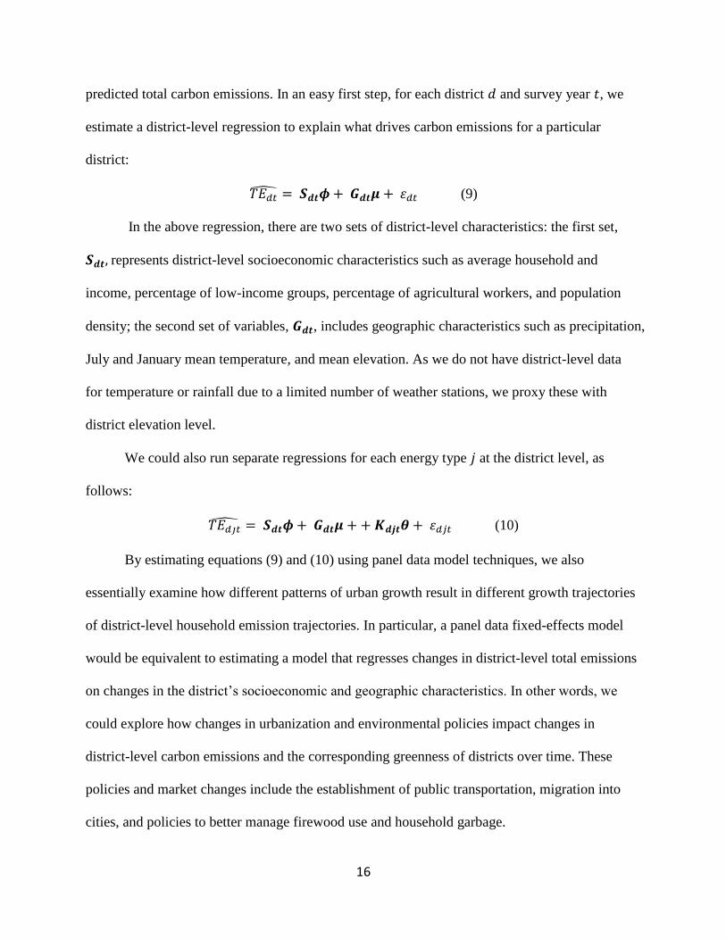
predicted total carbon emissions. In an easy first step, for each district 𝑑 and survey year 𝑡, we

estimate a district-level regression to explain what drives carbon emissions for a particular

district:

𝑇𝐸𝑑�� = 𝑺𝒅𝒕𝝓 + 𝑮𝒅𝒕𝝁 + 휀𝑑𝑡 (9)

In the above regression, there are two sets of district-level characteristics: the first set,

𝑺𝒅𝒕, represents district-level socioeconomic characteristics such as average household and

income, percentage of low-income groups, percentage of agricultural workers, and population

density; the second set of variables, 𝑮𝒅𝒕, includes geographic characteristics such as precipitation,

July and January mean temperature, and mean elevation. As we do not have district-level data

for temperature or rainfall due to a limited number of weather stations, we proxy these with

district elevation level.

We could also run separate regressions for each energy type 𝑗 at the district level, as

follows:

𝑇𝐸𝑑𝑗�� = 𝑺𝒅𝒕𝝓 + 𝑮𝒅𝒕𝝁 + + 𝑲𝒅𝒋𝒕𝜽 + 휀𝑑𝑗𝑡 (10)

By estimating equations (9) and (10) using panel data model techniques, we also

essentially examine how different patterns of urban growth result in different growth trajectories

of district-level household emission trajectories. In particular, a panel data fixed-effects model

would be equivalent to estimating a model that regresses changes in district-level total emissions

on changes in the district’s socioeconomic and geographic characteristics. In other words, we

could explore how changes in urbanization and environmental policies impact changes in

district-level carbon emissions and the corresponding greenness of districts over time. These

policies and market changes include the establishment of public transportation, migration into

cities, and policies to better manage firewood use and household garbage.

17

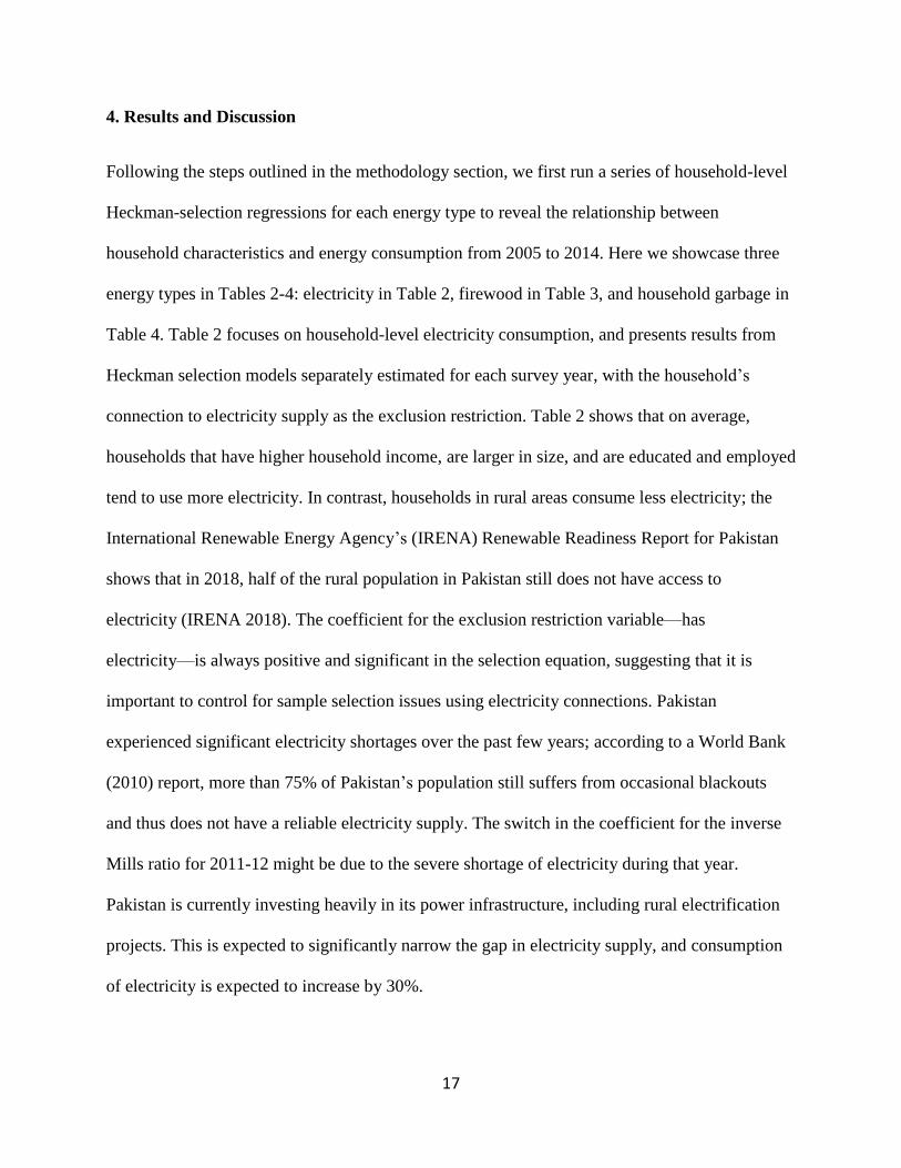
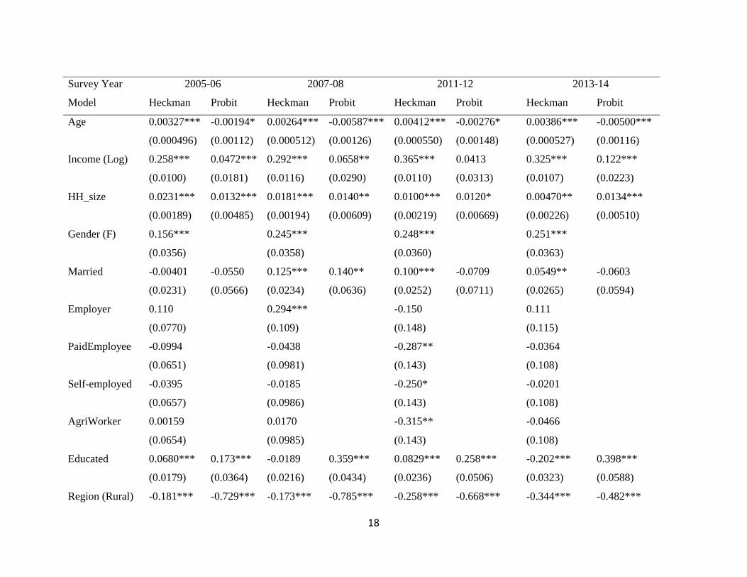
4. Results and Discussion

Following the steps outlined in the methodology section, we first run a series of household-level

Heckman-selection regressions for each energy type to reveal the relationship between

household characteristics and energy consumption from 2005 to 2014. Here we showcase three

energy types in Tables 2-4: electricity in Table 2, firewood in Table 3, and household garbage in

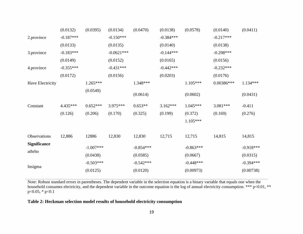
Table 4. Table 2 focuses on household-level electricity consumption, and presents results from

Heckman selection models separately estimated for each survey year, with the household’s

connection to electricity supply as the exclusion restriction. Table 2 shows that on average,

households that have higher household income, are larger in size, and are educated and employed

tend to use more electricity. In contrast, households in rural areas consume less electricity; the

International Renewable Energy Agency’s (IRENA) Renewable Readiness Report for Pakistan

shows that in 2018, half of the rural population in Pakistan still does not have access to

electricity (IRENA 2018). The coefficient for the exclusion restriction variable—has

electricity—is always positive and significant in the selection equation, suggesting that it is

important to control for sample selection issues using electricity connections. Pakistan

experienced significant electricity shortages over the past few years; according to a World Bank

(2010) report, more than 75% of Pakistan’s population still suffers from occasional blackouts

and thus does not have a reliable electricity supply. The switch in the coefficient for the inverse

Mills ratio for 2011-12 might be due to the severe shortage of electricity during that year.

Pakistan is currently investing heavily in its power infrastructure, including rural electrification

projects. This is expected to significantly narrow the gap in electricity supply, and consumption

of electricity is expected to increase by 30%.

18

Survey Year 2005-06 2007-08 2011-12 2013-14

Model Heckman Probit Heckman Probit Heckman Probit Heckman Probit

Age 0.00327*** -0.00194* 0.00264*** -0.00587*** 0.00412*** -0.00276* 0.00386*** -0.00500***

(0.000496) (0.00112) (0.000512) (0.00126) (0.000550) (0.00148) (0.000527) (0.00116)

Income (Log) 0.258*** 0.0472*** 0.292*** 0.0658** 0.365*** 0.0413 0.325*** 0.122***

(0.0100) (0.0181) (0.0116) (0.0290) (0.0110) (0.0313) (0.0107) (0.0223)

HH_size 0.0231*** 0.0132*** 0.0181*** 0.0140** 0.0100*** 0.0120* 0.00470** 0.0134***

(0.00189) (0.00485) (0.00194) (0.00609) (0.00219) (0.00669) (0.00226) (0.00510)

Gender (F) 0.156***

0.245***

0.248***

0.251***

(0.0356)

(0.0358)

(0.0360)

(0.0363)

Married -0.00401 -0.0550 0.125*** 0.140** 0.100*** -0.0709 0.0549** -0.0603

(0.0231) (0.0566) (0.0234) (0.0636) (0.0252) (0.0711) (0.0265) (0.0594)

Employer 0.110

0.294***

-0.150

0.111

(0.0770)

(0.109)

(0.148)

(0.115)

PaidEmployee -0.0994

-0.0438

-0.287**

-0.0364

(0.0651)

(0.0981)

(0.143)

(0.108)

Self-employed -0.0395

-0.0185

-0.250*

-0.0201

(0.0657)

(0.0986)

(0.143)

(0.108)

AgriWorker 0.00159

0.0170

-0.315**

-0.0466

(0.0654)

(0.0985)

(0.143)

(0.108)

Educated 0.0680*** 0.173*** -0.0189 0.359*** 0.0829*** 0.258*** -0.202*** 0.398***

(0.0179) (0.0364) (0.0216) (0.0434) (0.0236) (0.0506) (0.0323) (0.0588)

Region (Rural) -0.181*** -0.729*** -0.173*** -0.785*** -0.258*** -0.668*** -0.344*** -0.482***

19

Note: Robust standard errors in parentheses. The dependent variable in the selection equation is a binary variable that equals one when the

household consumes electricity, and the dependent variable in the outcome equation is the log of annual electricity consumption. *** p<0.01, **

p<0.05, * p<0.1

Table 2: Heckman selection model results of household electricity consumption

(0.0132) (0.0395) (0.0134) (0.0470) (0.0138) (0.0578) (0.0140) (0.0411)

2.province -0.187***

-0.150***

-0.384***

-0.217***

(0.0133)

(0.0135)

(0.0140)

(0.0138)


-0.0621***

-0.144***

-0.298***

(0.0149)

(0.0152)

(0.0165)

(0.0156)


-0.431***

-0.442***

-0.232***

(0.0172)

(0.0156)

(0.0203)

(0.0176)

Have Electricity

1.265***

1.348***

1.105*** 0.00386*** 1.134***

(0.0549)

(0.0614)

(0.0602)

(0.0431)

Constant 4.435*** 0.652*** 3.975*** 0.653** 3.162*** 1.045*** 3.081*** -0.411

(0.126) (0.206) (0.170) (0.325) (0.199) (0.372) (0.169) (0.276)

1.105***

Observations 12,886 12886 12,830 12,830 12,715 12,715 14,815 14,815

Significance

athrho

lnsigma

-1.007***

(0.0438)

-0.503***

(0.0125)

-0.854***

(0.0585)

-0.542***

(0.0120)

-0.863***

(0.0667)

-0.448***

(0.00973)

-0.918***

(0.0315)

-0.394***

(0.00738)

20

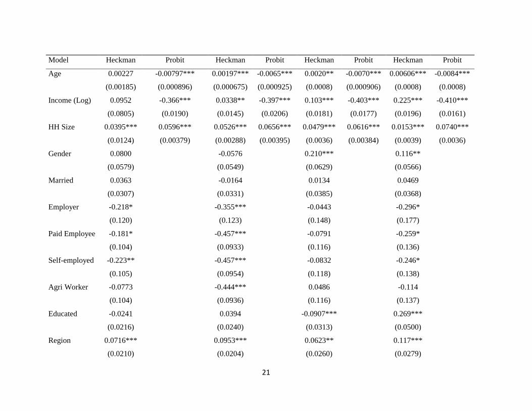
Tables 3 and 4 present results for two energy types that most previous studies overlook:

firewood and household garbage. Although households do not directly “consume” household

garbage, it essentially serves as a proxy for the consumption of food (kitchen waste), paper and

packing products, and a small quantity of recyclable items. Table 3 shows that households in

rural areas and with a larger household size consistently tend to use more firewood, In contrast,

households in which the head is either self-employed or works as a paid employee or agricultural

worker, as well as those with higher household income, consume less firewood in general.

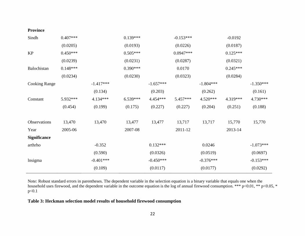
Interestingly, the selection equation shows that households with a cooking range are less

likely to use firewood. This is because such stoves usually use natural gas fuel, and hence

firewood is not used as cooking fuel. A comparison across all four provinces shows that

firewood use in rural provinces, such as Balochistan and KP, is much higher; this is consistent

with the aggregate statistic that in 2013-14, more than half of energy consumption in these two

rural provinces is still from firewood use. This situation is further aggravated when the provision

of natural gas is established in more urbanized provinces, such as KP and Sindh, owing to greater

political influence. In contrast, many households in the largely rural Balochistan province—

which contains the largest reservoirs of natural gas in Pakistan—lack access to natural gas.

Relative to natural gas, firewood and cow dung are often used by rural residents who do not have

a natural gas connection. Yet previous research on emission factors has demonstrated that

firewood and cow dung emit either too much carbon or other poisonous gases. Recently, the

carbon neutrality of firewood as a fuel has been argued; however, it is important to note that

when firewood is used, the rate of carbon emissions far exceeds the slow, decades-long carbon

sequestration process. In practice, therefore, firewood’s carbon neutrality remains wishful

thinking. According to Schlesinger (2018), carbon neutrality for wood can only be attained if

21

Model Heckman Probit Heckman Probit Heckman Probit Heckman Probit

Age 0.00227 -0.00797*** 0.00197*** -0.0065*** 0.0020** -0.0070*** 0.00606*** -0.0084***

(0.00185) (0.000896) (0.000675) (0.000925) (0.0008) (0.000906) (0.0008) (0.0008)

Income (Log) 0.0952 -0.366*** 0.0338** -0.397*** 0.103*** -0.403*** 0.225*** -0.410***

(0.0805) (0.0190) (0.0145) (0.0206) (0.0181) (0.0177) (0.0196) (0.0161)

HH Size 0.0395*** 0.0596*** 0.0526*** 0.0656*** 0.0479*** 0.0616*** 0.0153*** 0.0740***

(0.0124) (0.00379) (0.00288) (0.00395) (0.0036) (0.00384) (0.0039) (0.0036)

Gender 0.0800 -0.0576 0.210*** 0.116**

(0.0579) (0.0549) (0.0629) (0.0566)

Married 0.0363 -0.0164 0.0134 0.0469

(0.0307) (0.0331) (0.0385) (0.0368)

Employer -0.218* -0.355*** -0.0443 -0.296*

(0.120) (0.123) (0.148) (0.177)

Paid Employee -0.181* -0.457*** -0.0791 -0.259*

(0.104) (0.0933) (0.116) (0.136)

Self-employed -0.223** -0.457*** -0.0832 -0.246*

(0.105) (0.0954) (0.118) (0.138)

Agri Worker -0.0773 -0.444*** 0.0486 -0.114

(0.104) (0.0936) (0.116) (0.137)

Educated -0.0241 0.0394 -0.0907*** 0.269***

(0.0216) (0.0240) (0.0313) (0.0500)

Region 0.0716*** 0.0953*** 0.0623** 0.117***

(0.0210) (0.0204) (0.0260) (0.0279)

22

Note: Robust standard errors in parentheses. The dependent variable in the selection equation is a binary variable that equals one when the

household uses firewood, and the dependent variable in the outcome equation is the log of annual firewood consumption. *** p<0.01, ** p<0.05, *

p<0.1

Table 3: Heckman selection model results of household firewood consumption

Province

Sindh 0.407*** 0.139*** -0.153*** -0.0192

(0.0205) (0.0193) (0.0226) (0.0187)

KP 0.450*** 0.505*** 0.0947*** 0.125***

(0.0239) (0.0231) (0.0287) (0.0321)

Balochistan 0.148*** 0.390*** 0.0170 0.245***

(0.0234) (0.0230) (0.0323) (0.0284)

Cooking Range -1.417*** -1.657*** -1.804*** -1.350***

(0.134) (0.203) (0.262) (0.161)

Constant 5.932*** 4.134*** 6.539*** 4.454*** 5.457*** 4.520*** 4.319*** 4.730***

(0.454) (0.199) (0.175) (0.227) (0.227) (0.204) (0.251) (0.188)

Observations 13,470 13,470 13,477 13,477 13,717 13,717 15,770 15,770

Year 2005-06 2007-08 2011-12 2013-14

Significance

arthrho -0.352 0.132*** 0.0246 -1.073***

(0.590) (0.0326) (0.0519) (0.0697)

lnsigma -0.401*** -0.450*** -0.376*** -0.153***

(0.109) (0.0117) (0.0177) (0.0292)

23

Note: Robust standard errors in parentheses. *** p<0.01, ** p<0.05, * p<0.1

Table 4: Household Garbage Generation Determinants

VARIABLES Garbage Quantity Garbage Quantity Garbage Quantity Garbage Quantity

Age 9.22e-05 -4.39e-06 0.000124 0.000658**

(0.000293) (0.000278) (0.000271) (0.000259)

Income (Log) 0.0223*** 0.0256*** 0.0316*** 0.0403***

(0.00465) (0.00468) (0.00478) (0.00465)

HH_size 0.256*** 0.272*** 0.276*** 0.275***

(0.00108) (0.00108) (0.00108) (0.00105)

Gender (F) 0.134*** 0.132*** 0.141*** 0.118***

(0.0232) (0.0202) (0.0189) (0.0188)

Married 0.214*** 0.198*** 0.194*** 0.205***

(0.0137) (0.0131) (0.0128) (0.0130)

Employer 0.00650 -0.00432 0.0422 0.00658

(0.0514) (0.0611) (0.0678) (0.0600)

PaidEmployee 0.0607 0.0661 0.0612 -0.00674

(0.0466) (0.0536) (0.0642) (0.0557)

Self-employed 0.0584 0.0647 0.0531 -0.00595

(0.0470) (0.0539) (0.0644) (0.0561)

AgriWorker 0.0688 0.0629 0.0651 0.0102

(0.0467) (0.0537) (0.0644) (0.0559)

Educated -0.00446 0.00115 -0.0198* 0.00819

(0.0101) (0.0107) (0.0108) (0.0149)

Region (Rural) -0.545*** -0.530*** -0.563*** -0.561***

(0.00801) (0.00720) (0.00697) (0.00707)

2.province 0.0206** -0.0160** 0.0166** 0.0157**

(0.00866) (0.00787) (0.00732) (0.00704)

3.province 0.0194* 0.0322*** 0.0628*** 0.0698***

(0.0100) (0.00905) (0.00878) (0.00866)

4.province -0.0860*** -0.0743*** -0.130*** -0.0952***

(0.0109) (0.00954) (0.0111) (0.0106)

Constant 6.552*** 6.410*** 6.330*** 6.223***

(0.0701) (0.0758) (0.0859) (0.0798)

Observations 12,701 12,681 12,649 14,679

R-squared 0.853 0.868 0.875 0.867

Year 2005-06 2007-08 2010-11 2013-14

24

forest lands are managed to regrow such that they store more than their original biomass. In

addition, the benefit of wood energy must be discounted by the loss of carbon sequestration due

to deforestation. The rapid loss of forest cover in Pakistan renders the proposition even more

unviable here.

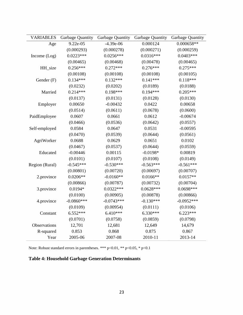
Table 4 presents the OLS regression of household garbage separately for each survey

year. We focus on household garbage because garbage collection by public and private agencies

is limited—and as IPCC (2006) guidelines indicate, open burning is a source of carbon emissions

that must be included in the national carbon emissions estimate. These regressions show that

households tend to generate more household garbage when they have higher household income,

are larger in size, and the head of the household is female. As stated previously, the average

household size in Pakistan is currently close to seven, and the country’s population is growing at

an annual rate of 2.4%, which suggests that household garbage in Pakistan will likely continue to

be an important issue. In contrast, households in rural areas tend to produce much less household

garbage, mainly due to the use of food waste and other recyclables for backyard livestock or

manure production. According to a World Migration Report (Hugo 2014) a key feature of Asian

megacities is that they include extensive peri-urban regions of mixed urban and rural land use,

but follow an urban life style—and hence could lead to a significant increase in household

garbage generation. Interestingly, better education seems to help reduce the generation of

household garbage, as can be seen from the 2010-11 survey regression results.

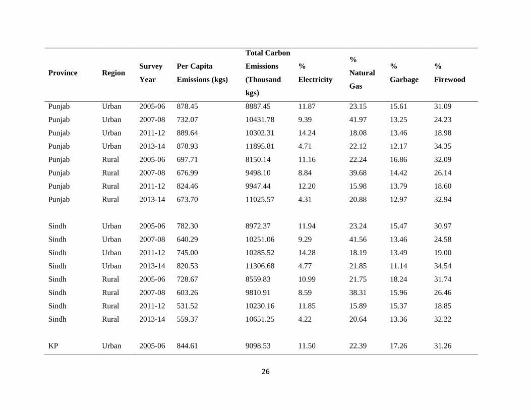
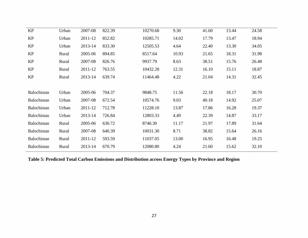
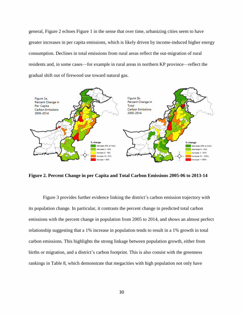
Table 5 presents average total and per capita predicted carbon emissions for both urban

and rural areas of all four provinces in Pakistan from 2004-05 to 2013-14. These carbon

emissions were predicted following steps (1)-(3) outlined in the methodology section by

applying household regression coefficients to province-level representative household

25

characteristics. In addition, the table also shows the share of total carbon emissions resulting

from firewood use and household garbage in 2013-14. This overall comparison across provinces

and urban-rural distinctions reveals several interesting findings: First, although total carbon

emissions from urban areas are significantly higher than those from rural areas—yet comparison

of per capita emissions shows that per capita carbon emissions across all urban residents are not

substantially higher than those for rural residents—suggests that differences in carbon emissions

are mostly due to population density. This is also confirmed by Figure 3, which shows that a 1%

increase in a district’s population will on average lead to a 1% increase in total carbon emissions.

Second, the urban areas of all four provinces have significantly lower proportions of carbon

emissions from firewood use than their rural counterparts. In general, from 2005 to 2014,

emissions from firewood use declined in most urban regions and in rural areas in Punjab and

Sindh provinces. However, carbon emissions from the firewood use in rural areas in the two

rural provinces, KP and Balochistan, are still more than 50% as of 2013-14.

A spatial study (Urban Unit 2018) based on labor force surveys for the years 2010-2015

indicates that the percentage of rural migrants in urban populations is highest in Punjab province

(7.5%), followed by Sindh (2%), KP (2%), and Balochistan (0.08%). Focusing on Punjab, the

districts of Lahore, Rawalpindi, and Faisalabad receive 23%, 17%, and 10% of the province’s

migrants, respectively. In the case of Lahore, 4% of migrants are from KP province. Looking at

Table 5, we can see that on average, urban to urban migration by a representative household

from KP to Punjab would not yield any significant change in emissions, whereas rural to urban

migration would increase emissions by 37% from 640 kgs per person for a rural resident in KP to

879 kgs for a Punjab urbanite. In the case of intra-provincial rural to urban migration in Sindh

province, emissions would rise by 6% assuming no change in household characteristics.

26

Province Region Survey

Year

Per Capita

Emissions (kgs)

Total Carbon

Emissions

(Thousand

kgs)

%

Electricity

%

Natural

Gas

%

Garbage

%

Firewood

Punjab Urban 2005-06 878.45 8887.45 11.87 23.15 15.61 31.09

Punjab Urban 2007-08 732.07 10431.78 9.39 41.97 13.25 24.23

Punjab Urban 2011-12 889.64 10302.31 14.24 18.08 13.46 18.98

Punjab Urban 2013-14 878.93 11895.81 4.71 22.12 12.17 34.35

Punjab Rural 2005-06 697.71 8150.14 11.16 22.24 16.86 32.09

Punjab Rural 2007-08 676.99 9498.10 8.84 39.68 14.42 26.14

Punjab Rural 2011-12 824.46 9947.44 12.20 15.98 13.79 18.60

Punjab Rural 2013-14 673.70 11025.57 4.31 20.88 12.97 32.94

Sindh Urban 2005-06 782.30 8972.37 11.94 23.24 15.47 30.97

Sindh Urban 2007-08 640.29 10251.06 9.29 41.56 13.46 24.58

Sindh Urban 2011-12 745.00 10285.52 14.28 18.19 13.49 19.00

Sindh Urban 2013-14 820.53 11306.68 4.77 21.85 11.14 34.54

Sindh Rural 2005-06 728.67 8559.83 10.99 21.75 18.24 31.74

Sindh Rural 2007-08 603.26 9810.91 8.59 38.31 15.96 26.46

Sindh Rural 2011-12 531.52 10230.16 11.85 15.89 15.37 18.85

Sindh Rural 2013-14 559.37 10651.25 4.22 20.64 13.36 32.22

KP Urban 2005-06 844.61 9098.53 11.50 22.39 17.26 31.26

27

KP Urban 2007-08 822.39 10270.68 9.30 41.60 13.44 24.58

KP Urban 2011-12 852.82 10285.71 14.02 17.79 13.47 18.94

KP Urban 2013-14 833.30 12505.53 4.64 22.40 13.30 34.05

KP Rural 2005-06 894.85 8517.64 10.93 21.65 18.31 31.98

KP Rural 2007-08 826.76 9937.79 8.63 38.51 15.76 26.48

KP Rural 2011-12 763.55 10432.28 12.31 16.10 15.11 18.87

KP Rural 2013-14 639.74 11464.48 4.22 21.04 14.31 32.45

Balochistan Urban 2005-06 704.37 9848.75 11.56 22.18 18.17 30.70




Balochistan Rural 2005-06 630.72 8746.30 11.17 21.97 17.89 31.64




Table 5: Predicted Total Carbon Emissions and Distribution across Energy Types by Province and Region

28

Heavy reliance on firewood for energy consumption could be a result of multiple factors,

including higher elevation, greater forest cover in mountainous areas, lower household income,

lack of access to cheaper alternatives such as natural gas, and weak enforcement of forest

protection. As explained above, the provision of natural gas is heavily geared toward the urban

provinces of Punjab and Sindh, even though Balochistan has the largest reservoirs of natural gas.

Finally, carbon emissions from household garbage account for more than 10% of all carbon

emissions for any specific district, and in particular, rural areas actually witnessed an increase in

carbon emissions from household garbage.

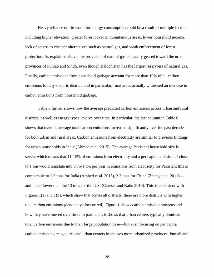
Table 6 further shows how the average predicted carbon emissions across urban and rural

districts, as well as energy types, evolve over time. In particular, the last column in Table 6

shows that overall, average total carbon emissions increased significantly over the past decade

for both urban and rural areas. Carbon emissions from electricity are similar to previous findings

for urban households in India (Ahmed et al. 2015): The average Pakistani household size is

seven, which means that 11-15% of emissions from electricity and a per capita emission of close

to 1 ton would translate into 0.75-1 ton per year in emissions from electricity for Pakistan; this is

comparable to 1.3 tons for India (Amhed et al. 2015), 2.3 tons for China (Zheng et al. 2011)—

and much lower than the 13 tons for the U.S. (Glaeser and Kahn 2010). This is consistent with

Figures 1(a) and 1(b), which show that across all districts, there are more districts with higher

total carbon emissions (denoted yellow or red). Figure 1 shows carbon emission hotspots and

how they have moved over time. In particular, it shows that urban centers typically dominate

total carbon emissions due to their large population base—but even focusing on per capita

carbon emissions, megacities and urban centers in the two more urbanized provinces, Punjab and

29

Sindh, contain the most emission hotspots. Notable outliers are the remote, higher-elevation rural

areas in northern KP province that depend on firewood for heating.

Figure 1. Total and per Capita Carbon Emissions by Districts for 2005-06 and 2013-14

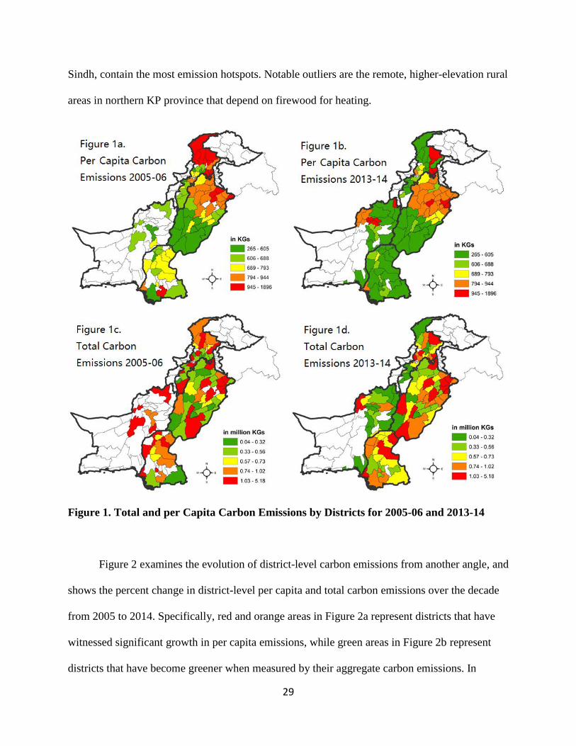
Figure 2 examines the evolution of district-level carbon emissions from another angle, and

shows the percent change in district-level per capita and total carbon emissions over the decade

from 2005 to 2014. Specifically, red and orange areas in Figure 2a represent districts that have

witnessed significant growth in per capita emissions, while green areas in Figure 2b represent

districts that have become greener when measured by their aggregate carbon emissions. In

30

general, Figure 2 echoes Figure 1 in the sense that over time, urbanizing cities seem to have

greater increases in per capita emissions, which is likely driven by income-induced higher energy

consumption. Declines in total emissions from rural areas reflect the out-migration of rural

residents and, in some cases—for example in rural areas in northern KP province—reflect the

gradual shift out of firewood use toward natural gas.

Figure 2. Percent Change in per Capita and Total Carbon Emissions 2005-06 to 2013-14

Figure 3 provides further evidence linking the district’s carbon emission trajectory with

its population change. In particular, it contrasts the percent change in predicted total carbon

emissions with the percent change in population from 2005 to 2014, and shows an almost perfect

relationship suggesting that a 1% increase in population tends to result in a 1% growth in total

carbon emissions. This highlights the strong linkage between population growth, either from

births or migration, and a district’s carbon footprint. This is also consist with the greenness

rankings in Table 8, which demonstrate that megacities with high population not only have

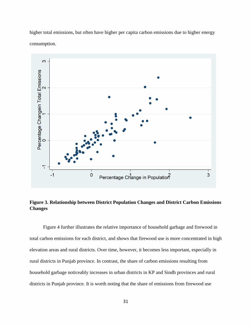
31

higher total emissions, but often have higher per capita carbon emissions due to higher energy

consumption.

Figure 3. Relationship between District Population Changes and District Carbon Emissions

Changes

Figure 4 further illustrates the relative importance of household garbage and firewood in

total carbon emissions for each district, and shows that firewood use is more concentrated in high

elevation areas and rural districts. Over time, however, it becomes less important, especially in

rural districts in Punjab province. In contrast, the share of carbon emissions resulting from

household garbage noticeably increases in urban districts in KP and Sindh provinces and rural

districts in Punjab province. It is worth noting that the share of emissions from firewood use

32

significantly increased from 2011-12 to 2013-14, but this is likely due to acute shortages in the

electricity supply. Similarly, the sharp increase in gasoline use by urban and rural residents in

2011-12 is a result of low energy prices.

Figure 4. Share of District Total Carbon Emissions from Firewood Use and Household

Garbage 2005-06 vs. 2013-14

Across the years, the major contributors to carbon emissions are firewood and natural gas

(20% each), and followed by household garbage and electricity each capturing less than 15%.

Focusing on the northwest tip of the country in Figure 4, we also notice a reduction in reliance

33

on firewood for heating in northern KP province, which is consistent with the lower-emissions

story illustrated in Figure 2.

The distribution of carbon emissions and energy consumptions across energy types varies

by districts. For example, gasoline consumption is heavily concentrated in urban cities such as

Karachi and Lahore, and disproportionately used by households with higher income or salary.

The role of public transportation is heterogeneous across cities: A ratio of predicted carbon

emissions from public transportation relative to private vehicle usage based on our analysis

shows that the proportion of carbon emissions from public transport to private transport is 30%

in Karachi, 16 % in Islamabad, and just 7% in Lahore in 2013–14. Figure 5 further contrasts per

capita carbon emissions for four types of districts based on their degree of urbanization: (a)

megacities with population greater than 1 million; (b) urban centers, in which the proportion of

urban households exceeds 50%; (c) emerging cities, in which the proportion of urban households

is in excess of the national average of 37% and less than 50%; and (d) rural areas. Figure 5

shows that these four district groups exhibit different trends over time: Emissions for megacities

show a U-shaped curve, which means that with increasing population—due to either natural

growth or migration—the marginal change in emissions is increasing. The emissions trend for

urban centers and emerging cities category is passing through a transition stage, due to energy

shortages and migration shocks, and rural areas show a declining trend of emissions due to

gradual improvement in the provision of cleaner fuels.

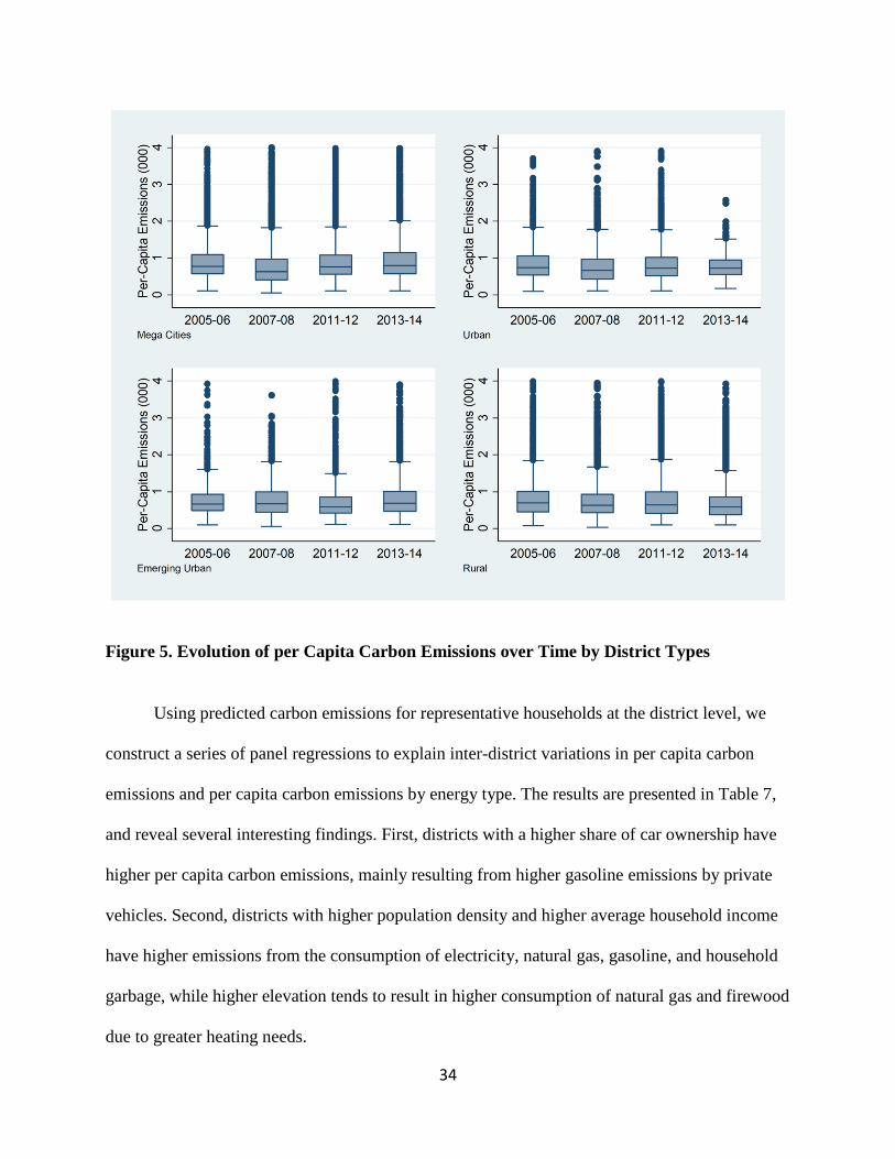
34

Figure 5. Evolution of per Capita Carbon Emissions over Time by District Types

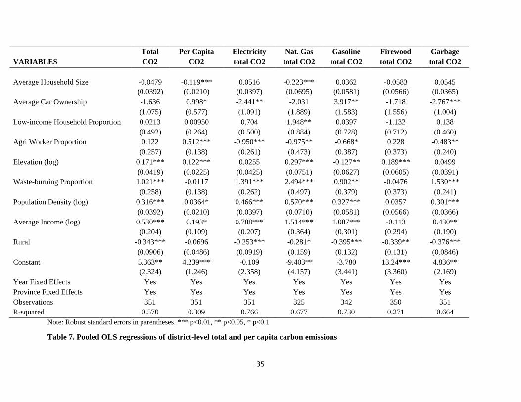
Using predicted carbon emissions for representative households at the district level, we

construct a series of panel regressions to explain inter-district variations in per capita carbon

emissions and per capita carbon emissions by energy type. The results are presented in Table 7,

and reveal several interesting findings. First, districts with a higher share of car ownership have

higher per capita carbon emissions, mainly resulting from higher gasoline emissions by private

vehicles. Second, districts with higher population density and higher average household income

have higher emissions from the consumption of electricity, natural gas, gasoline, and household

garbage, while higher elevation tends to result in higher consumption of natural gas and firewood

due to greater heating needs.

35

VARIABLES

Total

CO2

Per Capita

CO2

Electricity

total CO2

Nat. Gas

total CO2

Gasoline

total CO2

Firewood

total CO2

Garbage

total CO2

Average Household Size -0.0479 -0.119*** 0.0516 -0.223*** 0.0362 -0.0583 0.0545

(0.0392) (0.0210) (0.0397) (0.0695) (0.0581) (0.0566) (0.0365)

Average Car Ownership -1.636 0.998* -2.441** -2.031 3.917** -1.718 -2.767***

(1.075) (0.577) (1.091) (1.889) (1.583) (1.556) (1.004)

Low-income Household Proportion 0.0213 0.00950 0.704 1.948** 0.0397 -1.132 0.138

(0.492) (0.264) (0.500) (0.884) (0.728) (0.712) (0.460)

Agri Worker Proportion 0.122 0.512*** -0.950*** -0.975** -0.668* 0.228 -0.483**

(0.257) (0.138) (0.261) (0.473) (0.387) (0.373) (0.240)

Elevation (log) 0.171*** 0.122*** 0.0255 0.297*** -0.127** 0.189*** 0.0499

(0.0419) (0.0225) (0.0425) (0.0751) (0.0627) (0.0605) (0.0391)

Waste-burning Proportion 1.021*** -0.0117 1.391*** 2.494*** 0.902** -0.0476 1.530***

(0.258) (0.138) (0.262) (0.497) (0.379) (0.373) (0.241)

Population Density (log) 0.316*** 0.0364* 0.466*** 0.570*** 0.327*** 0.0357 0.301***

(0.0392) (0.0210) (0.0397) (0.0710) (0.0581) (0.0566) (0.0366)

Average Income (log) 0.530*** 0.193* 0.788*** 1.514*** 1.087*** -0.113 0.430**

(0.204) (0.109) (0.207) (0.364) (0.301) (0.294) (0.190)

Rural -0.343*** -0.0696 -0.253*** -0.281* -0.395*** -0.339** -0.376***

(0.0906) (0.0486) (0.0919) (0.159) (0.132) (0.131) (0.0846)

Constant 5.363** 4.239*** -0.109 -9.403** -3.780 13.24*** 4.836**

(2.324) (1.246) (2.358) (4.157) (3.441) (3.360) (2.169)

Year Fixed Effects Yes Yes Yes Yes Yes Yes Yes

Province Fixed Effects Yes Yes Yes Yes Yes Yes Yes

Observations 351 351 351 325 342 350 351

R-squared 0.570 0.309 0.766 0.677 0.730 0.271 0.664

Note: Robust standard errors in parentheses. *** p<0.01, ** p<0.05, * p<0.1

Table 7. Pooled OLS regressions of district-level total and per capita carbon emissions

36

Third, higher-income districts typically have more total and per capita carbon emissions, and

hence could potentially benefit from more carbon abatement efforts. Finally, rural households

contribute significantly less from household garbage due to better utilization of most household

waste items as fodder for cattle. Figures 1 and 2 also confirm regional variations. For example,

Pakistan’s capital city, Islamabad, has the highest emissions from electricity and natural gas

usage because of urbanization, high affluence, and a relatively abundant energy supply. In

contrast, districts located in mountainous regions such as KP province rely heavily on firewood

in their energy portfolio.

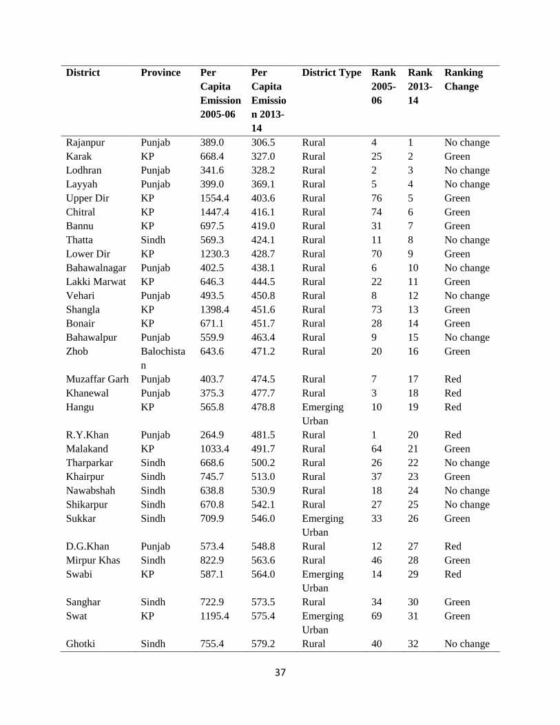
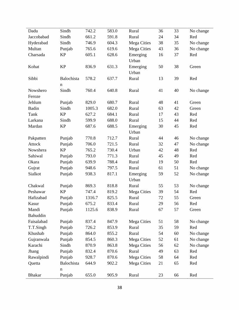
Finally, we ranked districts’ greenness based on the level of per capita carbon emissions

for each survey year, and assign a higher ranking if the district has lower carbon emissions and

thus is greener. Table 8 presents per capita emissions for 2005-06 and 2013-14, greenness

rankings for 2013-14, and an indicator for change in the district’s ranking from 2005 to 2014. In

particular, for every survey year, we ranked all districts and divide them into five quintiles. We

label a district as “no change” if it stays within the same greenness quintile from 2005 to 2014,

“red” if it emits significantly higher per capita emissions and moves to a lower quintile in 2013-

14 compared to the previous decade, and “green” if the district moves up by at least one quintile

in its greenness ranking. For example, the Karak district in KP province had per capita carbon

emissions of 668 kg in 2005-06 and a greenness ranking of 25 out of all 77 districts that were

surveyed every year from 2005 to 2014. In 2013-14, it managed to cut its per capita emissions by

half because of increased provision of natural gas and better municipal services. Its current rank

is 2, and thus is labeled green.

37

District Province Per

Capita

Emission

2005-06

Per

Capita

Emissio

n 2013-

14

District Type Rank

2005-

06

Rank

2013-

14

Ranking

Change

Rajanpur Punjab 389.0 306.5 Rural 4 1 No change

Karak KP 668.4 327.0 Rural 25 2 Green

Lodhran Punjab 341.6 328.2 Rural 2 3 No change

Layyah Punjab 399.0 369.1 Rural 5 4 No change

Upper Dir KP 1554.4 403.6 Rural 76 5 Green

Chitral KP 1447.4 416.1 Rural 74 6 Green

Bannu KP 697.5 419.0 Rural 31 7 Green

Thatta Sindh 569.3 424.1 Rural 11 8 No change

Lower Dir KP 1230.3 428.7 Rural 70 9 Green

Bahawalnagar Punjab 402.5 438.1 Rural 6 10 No change

Lakki Marwat KP 646.3 444.5 Rural 22 11 Green

Vehari Punjab 493.5 450.8 Rural 8 12 No change

Shangla KP 1398.4 451.6 Rural 73 13 Green

Bonair KP 671.1 451.7 Rural 28 14 Green

Bahawalpur Punjab 559.9 463.4 Rural 9 15 No change

Zhob Balochista

n

643.6 471.2 Rural 20 16 Green

Muzaffar Garh Punjab 403.7 474.5 Rural 7 17 Red

Khanewal Punjab 375.3 477.7 Rural 3 18 Red

Hangu KP 565.8 478.8 Emerging

Urban

10 19 Red

R.Y.Khan Punjab 264.9 481.5 Rural 1 20 Red

Malakand KP 1033.4 491.7 Rural 64 21 Green

Tharparkar Sindh 668.6 500.2 Rural 26 22 No change

Khairpur Sindh 745.7 513.0 Rural 37 23 Green

Nawabshah Sindh 638.8 530.9 Rural 18 24 No change

Shikarpur Sindh 670.8 542.1 Rural 27 25 No change

Sukkar Sindh 709.9 546.0 Emerging

Urban

33 26 Green

D.G.Khan Punjab 573.4 548.8 Rural 12 27 Red

Mirpur Khas Sindh 822.9 563.6 Rural 46 28 Green

Swabi KP 587.1 564.0 Emerging

Urban

14 29 Red

Sanghar Sindh 722.9 573.5 Rural 34 30 Green

Swat KP 1195.4 575.4 Emerging

Urban

69 31 Green

Ghotki Sindh 755.4 579.2 Rural 40 32 No change

38

Dadu Sindh 742.2 583.0 Rural 36 33 No change

Jaccobabad Sindh 661.2 591.8 Rural 24 34 Red

Hyderabad Sindh 746.9 604.3 Mega Cities 38 35 No change

Multan Punjab 765.6 619.6 Mega Cities 43 36 No change

Charsada KP 605.1 628.6 Emerging

Urban

16 37 Red

Kohat KP 836.9 631.3 Emerging

Urban

50 38 Green

Sibbi Balochista

n

578.2 637.7 Rural 13 39 Red

Nowshero

Feroze

Sindh 760.4 640.8 Rural 41 40 No change

Jehlum Punjab 829.0 680.7 Rural 48 41 Green

Badin Sindh 1005.3 682.0 Rural 63 42 Green

Tank KP 627.2 684.1 Rural 17 43 Red

Larkana Sindh 599.9 688.0 Rural 15 44 Red

Mardan KP 687.6 688.5 Emerging

Urban

30 45 Red

Pakpatten Punjab 770.8 712.7 Rural 44 46 No change

Attock Punjab 706.0 721.5 Rural 32 47 No change

Nowshera KP 765.2 730.4 Urban 42 48 Red

Sahiwal Punjab 793.0 771.3 Rural 45 49 Red

Okara Punjab 639.9 788.4 Rural 19 50 Red

Gujrat Punjab 948.6 797.5 Rural 61 51 No change

Sialkot Punjab 938.3 817.1 Emerging

Urban

59 52 No change

Chakwal Punjab 869.3 818.8 Rural 55 53 No change

Peshawar KP 747.4 819.2 Mega Cities 39 54 Red

Hafizabad Punjab 1316.7 825.5 Rural 72 55 Green

Kasur Punjab 675.2 833.4 Rural 29 56 Red

Mandi

Bahuddin

Punjab 1125.6 838.9 Rural 67 57 Green

Faisalabad Punjab 837.4 847.9 Mega Cities 51 58 No change

T.T.Singh Punjab 726.2 853.9 Rural 35 59 Red

Khushab Punjab 864.0 855.2 Rural 54 60 No change

Gujranwala Punjab 854.5 860.3 Mega Cities 52 61 No change

Karachi Sindh 870.9 863.8 Mega Cities 56 62 No change

Jhang Punjab 832.4 870.6 Rural 49 63 Red

Rawalpindi Punjab 928.7 870.6 Mega Cities 58 64 Red

Quetta Balochista

n

644.9 902.2 Mega Cities 21 65 Red

Bhakar Punjab 655.0 905.9 Rural 23 66 Red

39

Mianwali Punjab 857.5 921.4 Rural 53 67 Red

Narowal Punjab 1297.5 928.4 Rural 71 68 No change

Sargodha Punjab 944.5 933.9 Emerging

Urban

60 69 Red

Sheikhupura Punjab 828.2 987.4 Emerging

Urban

47 70 Red

Kohistan KP 1895.7 995.9 Rural 77 71 No change

Haripur KP 1140.0 1079.4 Rural 68 72 No change

Lahore Punjab 901.8 1089.3 Mega Cities 57 73 Red

Manshera KP 1093.2 1097.8 Rural 66 74 No change

Batagram KP 1463.6 1147.2 Rural 75 75 No change

Abbotabad KP 950.1 1182.0 Emerging

Urban

62 76 Red

Islamabad Punjab 1056.6 1275.0 Mega Cities 65 77 No change

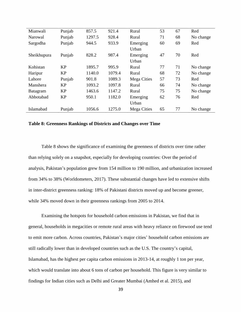
Table 8: Greenness Rankings of Districts and Changes over Time

Table 8 shows the significance of examining the greenness of districts over time rather

than relying solely on a snapshot, especially for developing countries: Over the period of

analysis, Pakistan’s population grew from 154 million to 190 million, and urbanization increased

from 34% to 38% (Worldometers, 2017). These substantial changes have led to extensive shifts

in inter-district greenness ranking: 18% of Pakistani districts moved up and become greener,

while 34% moved down in their greenness rankings from 2005 to 2014.

Examining the hotspots for household carbon emissions in Pakistan, we find that in

general, households in megacities or remote rural areas with heavy reliance on firewood use tend

to emit more carbon. Across countries, Pakistan’s major cities’ household carbon emissions are

still radically lower than in developed countries such as the U.S. The country’s capital,

Islamabad, has the highest per capita carbon emissions in 2013-14, at roughly 1 ton per year,

which would translate into about 6 tons of carbon per household. This figure is very similar to

findings for Indian cities such as Delhi and Greater Mumbai (Amhed et al. 2015), and

40

comparable to the Chinese cities study, which finds that Shanghai’s standardized household

produces 1.8 tons of carbon and Beijing’s produces 4 tons (Zheng et al. 2011). However,

Glaeser and Kahn (2010) report that in the cleanest U.S. cities (San Diego and San Francisco), a

standardized household emits around 26 tons of CO2 per year. This means that even in

Pakistan’s brownest city, Islamadad, a standardized household emits only one-fourth the carbon

produced by a standardized household in America’s greenest cities.

The city with the highest total carbon emissions is Karachi, followed by Lahore; these are

the only megacities with more than 10 million residents. The city with the third highest carbon

emissions is Peshawar. Peshawar is ranked sixth in population size, so we can safely assume that

the emissions trend is not entirely driven by population size; some spatial heterogeneity beyond

population size exists that provides a margin for policy intervention. Similarly, Quetta is ranked

fifth for emissions, but the tenth for population size. Rural-urban migration will convert

firewood use to cleaner alternatives, but residents in urban areas tend to have higher emissions

due to higher income-driven consumption, which suggests a possible significant increase in

Pakistan’s carbon emissions due to ongoing and massive migration into cities.

5. Conclusions

Using four rounds of nationwide household surveys for both rural and urban districts in Pakistan,

we provide the first empirical estimate of Pakistan’s household carbon emissions from use of all

energy types from 2005 to 2014 and examine the evolution of greenness rankings over time for

each district. Our main results reveal that except for high-elevation rural districts in KP province,

urban centers, and especially larger cities, represent the hotspots of household carbon emissions

in Pakistan even when measured as per capita emissions. This suggests future increases in

41

emissions for Pakistan, which faces massive rural to urban migration and rapid population

growth. In addition, we find that firewood use accounts for half of all carbon emissions across

households’ energy consumption in rural provinces, and ignoring household garbage would lead

to a 10% underestimate of household carbon emissions, especially for cities. Finally, our analysis

shows that 20% of Pakistani districts changed their greenness rankings by at least one quintile

from 2005 to 2014. This suggests that it is not advisable to rely solely on a single year’s survey

data, especially for developing countries like Pakistan that experience pressure from urbanization

and population growth.

Our paper makes several important contributions to the literature of sustainable

development, carbon accounting, and the interplay between urbanization, energy use, and carbon

emissions, and has important policy implications for adaptations to climate change, especially in

the developing world. By focusing on Pakistan—the sixth most populous country in the world—

and firewood, which is the main energy source for two billion people in lower-income

developing countries, our analysis highlights the importance of focusing on the often-overlooked

developing countries when analyzing the impacts of climate change. Although Pakistan currently

only accounts for 1% of global carbon emissions, it will be more significant in the decades to

come due to its rapid population growth and urbanization. More importantly, a better

understanding of the trajectory of carbon emissions for Pakistani cities and rural areas offers

more transferrable insights for countries in Africa and Latin America than insights from

developed countries. For example, the role of biomass fuel, especially firewood, in rural

households’ energy portfolios and its climate change impacts warrant more research in the future.

Furthermore, changes in the greenness rankings of 52% of Pakistani districts within one decade

confirms the importance of monitoring the climate profiles of a district, region, and country over

42

time, especially for urbanizing developing countries. In addition, our results reveal the uneven

distribution of reliable energy supply and climate impacts, which often have disproportionately

larger impacts on rural households that tend to have lower access to cheaper and consistent

alternative energy or abatement technologies. Finally, imminent carbon emissions from Pakistan

and similar developing countries merit further analysis for at least two reasons. First, a recent

study in China reveals that households’ energy consumption will likely increase with higher

temperatures (Li et al. 2018); this is likely also true for Pakistan, because it is one of the

countries that face the most significant climate risks. Second, ongoing projects, such as coal

power plants along the China Pakistan Economic Corridor, are projected to significantly alter

Pakistan’s energy consumption and carbon emissions profile.

Our analysis is not without limitations. First, because the PSLM surveys only have data on

self-reported energy expenditures rather than the quantity of consumption, we had to use

province-level energy prices to convert these measures, then use national-level emission

conversion factors to derive corresponding predicted carbon emissions. These conversions and

aggregations likely introduced measurement errors in our estimates, but a comparison between

the aggregate amount of our predicted energy consumption with official government statistics on

energy use at the province level reveals that our measures are within 5% of these statistics.

Second, Pakistan experienced significant electricity blackouts and shortages, especially in 2013-

14, which forced many households to use firewood. This could result in an artificially higher

share of carbon emissions from firewood due to unreliable electricity or natural gas supply,

which may not translate to all developing countries. Finally, PSLM surveys did not always cover

the same districts. Out of 100-some districts, however, we were able to match the majority; 77

districts were surveyed in all four rounds. Finally, our results—especially for remote rural

43

areas—might not be statistically representative if the poorest or most remote areas were less

likely to be surveyed.

44

References

ADB (2018). Sector Assistance Program Evaluation (SAPE) for the Pakistan Power Sector.

Asian Development Bank. Retrieved from

https://www.adb.org/sites/default/files/evaluation-document/397216/files/eap-pak-spe-

energy.pdf

Ahmad, S., Baiocchi, G., & Creutzig, F. (2015). CO2 Emissions from Direct Energy Use of

Urban Households in India. Environmental Science & Technology, 49, 11312−11320

Baiocchi, G., Minx, J., & Hubacek, K. (2010). The impact of social factors and consumer

behavior on carbon dioxide emissions in the United Kingdom: A regression based on

input− output and geodemographic consumer segmentation data. Journal of Industrial

Ecology, 14(1), 50-72.

Chavez, A., Ramaswami, A., Nath, D., Guru, R., & Kumar, E. (2012). Implementing trans‐

boundary infrastructure‐based greenhouse gas accounting for Delhi, India: Data

availability and methods. Journal of Industrial Ecology, 16(6), 814-828.

Chen, J., Kosec, K., & Mueller, V. (2019). Moving to despair? Migration and well-being in

Pakistan. World Development, 113, 186-203.

Craig, T. (2014, February 2). Energy shortages force Pakistanis to scavenge for wood,

threatening tree canopy. The Washington Post

Dewees, P. A. (1989) The Wood fuel Crisis Reconsidered: Observations on the Dynamics of

Abundance and Scarcity. World Development, 17:8, 1159–1172.

Dhakal, S. (2009). Urban energy use and carbon emissions from cities in China and policy

implications. Energy policy, 37(11), 4208-4219.

https://www.adb.org/sites/default/files/evaluation-document/397216/files/eap-pak-spe-energy.pdf

https://www.adb.org/sites/default/files/evaluation-document/397216/files/eap-pak-spe-energy.pdf

45

Ellis, P.; Roberts, M. (2016). Leveraging Urbanization in South Asia: Managing Spatial

Transformation for Prosperity and Livability. Washington, DC: World Bank.

Food and Agriculture Organization of the United Nations (FAO). (2017). The Future of Food

and Agriculture. Trends and Challenges.

Glaeser, E. L. & Kahn, M. E. (2010). The Greenness of Cities: Carbon Dioxide Emissions and

Urban Development. Journal of Urban Economics, 67(3), pp. 404- 18.

Han, X., & Chatterjee, L. (1997). Impacts of growth and structural change on CO2 emissions of

developing countries. World Development, 25(3), 395-407.

Heckman, J. J. (1976). The common structure of statistical models of truncation, sample

selection and limited dependent variables and a simple estimator for such models.

In Annals of Economic and Social Measurement, Volume 5, number 4 (pp. 475-492).

NBER.

Hugo, G. (2014). Urban migration trends, challenges, responses and policy in the Asia–Pacific.

World Migration Report, 2015. The University of Adelaide, Australia. International

Organization for Migration (IOM).

Hertwich, E. G., & Peters, G. P. (2009). Carbon footprint of nations: A global, trade-linked

analysis. Environmental science & technology, 43(16), 6414-6420.

Hydrocarbon Development Institute of Pakistan. Pakistan energy yearbook 2012 & 2014.

Islamabad: Ministry of Petroleum and Natural Resources.

International Energy Agency (2016) World Energy Outlook 2016. Paris: International Energy

Agency.

IRENA (2018). Renewable Readiness Assessment, Pakistan. International Renewable Energy

Agency

46

International Energy Agency, ‘IEA - Pakistan: Alternative and Renewable Energy Policy, 2011

(Medium Term Policy)’, 2016,

Jan, I., H. Khan, and S. Hayat (2012) Determinants of Rural Household Energy Choices: An

Example from Pakistan. Polish Journal of Environmental Studies 21:2, 635–641

Kahn, Matthew E. (2009) Urban Growth and Climate Change. Annual Review of Resource

Economics, pp. 333-49.

Kedir, M., Schmidt, E., & Wagas, A. (2016). Pakistan’s changing demography: Urbanization and

peri-urban transformation over time (Vol. 39). International Food Policy Research

Institute, Washington, DC.

Kreft, S., Eckstein, D., Dorsch, L., & Fischer, L. (2015). Global climate risk index 2016: who

suffers most from extreme weather events? Weather-related loss events in 2014 and 1995

to 2014. Germanwatch Nord-Süd Initiative

Kugelman, M. (Ed.). (2015). Pakistan's Interminable Energy Crisis: Is There Any Way Out?.

Woodrow Wilson International Center for Scholars.

Levitt, C. J., Saaby, M., & Sørensen, A. (2017). Australia's consumption‐based greenhouse gas

emissions. Australian Journal of Agricultural and Resource Economics, 61(2), 211-231.

Li, Y., W.A. Pizer, L. Wu. (2018). Climate change and residential electricity consumption in the

Yangtze River Delta, China. Proceedings of the National Academy of Sciences

Lipinski, B., Hanson, C., Lomax, J., Kitinoja, L., Waite, R., & Searchinger, T. (2013). Reducing

food loss and waste. World Resources Institute, 22. Lipinski, B., Hanson, C., Lomax, J.,

Kitinoja, L., Waite, R., & Searchinger, T. (2013). Reducing food loss and waste. World

Resources Institute, 22.

47

Minx, J., Baiocchi, G., Wiedmann, T., Barrett, J., Creutzig, F., Feng, K., ... & Hubacek, K.

(2013). Carbon footprints of cities and other human settlements in the UK.

Environmental Research Letters, 8(3), 035039.

National Electric Power Regularity Authority (NEPRA), Government of Pakistan. (2016). State

of industry report 2016.

Pakistan Economic Survey. (2014). Highlights of Pakistan Economic Survey 2014-15. Pakistan

Bureau of Statistics, Government of Pakistan

PSLM (2014). Pakistan Social and Living Standards Measurements Survey, 2013-14,

Government of Pakistan, Islamabad (2014). Available at

http://www.pbs.gov.pk/content/microdata

PSLM (2016). Pakistan Social and Living Standards Measurements Survey, 2015-16,

Government of Pakistan, Islamabad (2016)

Pakistan Today (2018, December 26). Climate change cost Pakistan Rs14bn in last 20 years:

PM’s advisor. Pakistan Today

Rees, W. E. (2006). Ecological footprints and bio capacity: Essential elements in sustainability

assessment. Renewables‐Based Technology: Sustainability Assessment, 143-157.

Salam, A. (2018, July 24). Pakistan is ground zero for global warming consequences. USA Today.

Sajjad, S. H., Blond, N., Batool, R., Shirazi, S. A., Shakrullah, K., & Bhalli, M. N. (2015). Study

of urban heat island of Karachi by using finite volume mesoscale model. Journal of Basic

and Applied Sciences, 11, 101-105.

Sanchez-Triana, E., Enriquez, S., Afzal, J., Nakagawa, A., & Khan, A. S. (2014). Cleaning

Pakistan's Air: Policy Options to Address the Cost of Outdoor Air Pollution. The World

48

Bank. Seriño, M. N. V., & Klasen, S. (2015). Estimation and determinants of the

Philippines' household carbon footprint. The Developing Economies, 53(1), 44-62.

Schlesinger, W. H. (2018). Are wood pellets a green fuel? Science, 359(6382), 1328–1329.

Seto, K. C., Dhakal, S., Bigio, A., Blanco, H., Delgado, G. C., Dewar, D., Huang, L., Inaba, A.,

Kansal, A., Lwasa, S., McMahon, J. E., Muller, D. B., Murakami, J., Nagendra, H.,

Ramaswami, A. (2014). Human Settlements, Infrastructure and Spatial Planning. In

Climate Change 2014: Mitigation of Climate Change. Contribution of Working Group III

to the Fifth Assessment Report of the Intergovernmental Panel on Climate Change,

Edenhofer, O., Pichs-Madruga, R., Sokona, Y., Farahani, E., Kadner, S., Seyboth, K.,

Adler, A., Baum, I., Brunner, S., Eickemeier, P., Kriemann, B., Savolainen, J., S.

Schlomer, C., von Stechow, Zwickel, T., Minx, J. C., Eds., Cambridge University Press:

Cambridge, United Kingdom.

Sustainable energy for all and Ministry of Finance - Implementation and Economic Reforms

Unit (IERU), ‘Pakistan: Rapid Assessment and Gap Analysis’, 2014, 15,

http://www.se4all.org/sites/default/files/Pakistan_RAGA_EN_Released.pdf.

United Nations (UN). (2014). World's population increasingly urban with more than half living

in urban areas.

Urban Unit (2018). Punjab Spatial Strategy. Planning and Development Department,

Government of Punjab. Retrieved from

http://urbanunit.gov.pk/Upload/Photos/Punjab%20Spatial%20Strategy.pdf

World Bank. (2010). Cities and climate change: an urgent agenda

World Bank Group. (2016). World development indicators 2016. World Bank Publication

49

World Bank. (2017). Pakistan off-grid lighting consumer perceptions: study overview (English).

Washington, D.C. World Bank Group. Retrieved from

http://documents.worldbank.org/curated/en/865301486382674587/Pakistan-off-grid-

lighting-consumer-perceptions-study-overview

Worldometers. (2017). Countries in the world by population.

Zhang, Z. (2000). Decoupling China’s carbon emissions increase from economic growth: An

economic analysis and policy implications. World Development, 28(4), 739-752.

Zheng, S., Wang R., Glaeser, E., & Kahn, M. (2011). The greenness of China: household carbon

dioxide emissions and urban development. Journal of Economic Geography, 11(5), 761-

792.

The Greenness of Rural and Urban Pakistan Over Time ...

Documents

Transcript of The Greenness of Rural and Urban Pakistan Over Time ...