209

IDŐJÁRÁS Quarterly Journal of the Hungarian Meteorological Service

Vol. 108, No. 4, October–December 2004, pp. 209–251

The greenhouse effect and the spectral decomposition of the clear-sky terrestrial radiation

Ferenc M. Miskolczi*1 and Martin G. Mlynczak2

1Analytical Services & Materials Inc.,

One Enterprise Parkway, Suite 300 Hampton, VA 23666, U.S.A. E-mail: f.m.miskolczi@larc.nasa.gov

2NASA Langley Research Center, Mail Stop 420, Hampton, VA 23681-2199, U.S.A. E-mail: m.g.mlynczak@larc.nasa.gov

(Manuscript received March 8, 2004; in final form November 1, 2004)

Abstract—In this paper the clear-sky infrared radiation field of the Earth-atmosphere system is characterized by the spectral decomposition of the simulated upward and downward flux density components into three distinct wave number regions. The relative contributions of the far infrared, middle infrared, and windows spectral regions to the total longwave flux densities have been established. The approximate qualitative description of the meridional distributions of the zonal averages gave us a detailed insight into the role of the less explored far infrared spectral region. We demonstrate that on a global scale, the far infrared contribution to the clear-sky normalized greenhouse factor is significantly increasing toward the polar regions. Accurate computation of the transmitted and re-emitted part of the outgoing longwave radiation showed that in the far infrared the normalized upward atmospheric emittance increases poleward. This phenomenon is the direct consequence of the downward shift of the peak of the weighting functions in the strongly absorbing opaque spectral regions. The clear-sky total longwave terrestrial flux transmittance seems to be well correlated with the far infrared flux transmittance, which implies the possibility of inferring total longwave flux densities solely from far infrared observations. The zonal averages of the total normalized atmospheric upward emittances are almost independent of the water vapor column amount, they have no meridional variation, and they are constantly about fifty percent of the surface upward flux density, an indication, that the gray atmosphere in the IR is in radiative equilibrium. The meridional distribution of the greenhouse temperature change and its dependence on the atmospheric water vapor content were also evaluated. Solving the Schwarzschild-Milne equations for the bounded atmosphere the infrared atmospheric transfer and greenhouse functions were derived. The theoretically predicted greenhouse effect in the clear atmosphere is in perfect agreement with simulation results and measurements. Key-words: greenhouse effect, radiative equilibrium, far infrared.

* Corresponding author. Tel: 757-827-4627; Fax: 757-825-8659

210

1. Introduction Terrestrial radiation or outgoing longwave radiation (OLR) are terms which refer to the emitted infrared (IR) radiation field of the Earth-atmosphere system. An accurate knowledge of the spatial and temporal distribution of this radiation field is fundamental in climate research. When long-term radiative equilibrium between the solar and terrestrial radiation exists monitoring the OLR one can identify the changes in the shortwave net input into the Earth-atmosphere system. From the satellite observation of the Earth’s radiation budget (ERBE, 2004) we estimated that the five years average effective planetary temperature is about 253.8 K. When using the observed albedo and a solar constant of 1365 W m–2, this results in an effective temperature of 253.0 K. Despite the fact that the average net radiation is off by about 5 W m–2, these results support the idea of the long-term radiative equilibrium.

The knowledge of the spectral characteristic of the OLR is equally important. Keeping the OLR constant, climate change might occur by changing the concentration of the greenhouse gases. Any change in the longwave atmospheric transparency will alter the contribution of the different spectral intervals to the OLR. For example, increased spectral OLR in the window regions coupled with constant total OLR and surface emissivity will point to an amplified greenhouse effect due to increased greenhouse gas concentration.

In principle, the classification of the spectral intervals of the terrestrial radiation must be based on observations of the spectral characteristics of the OLR or the downward atmospheric emittance (ED). So far the spectral boundaries of the far infrared (FIR), middle infrared (MIR), and windows (WIN) spectral regions are not exactly defined and there is no convention accepted by the scientific community regarding these boundaries. This is primarily because in the highly variable atmosphere, the exact wavelength of the complete absorption is changing. Sometimes, due to technical or engineering constraints, the spectral sensitivity of a detector or instrument design sets the spectral boundaries. However, focusing on the spectral aspects of the Earth's radiation budget or climate change, such definitions sooner or later will be necessary. Until then, meaningful quantitative comparisons of FIR, MIR, and WIN flux densities, cooling rates, greenhouse factors, or other spectrally resolved quantities from different authors will be difficult.

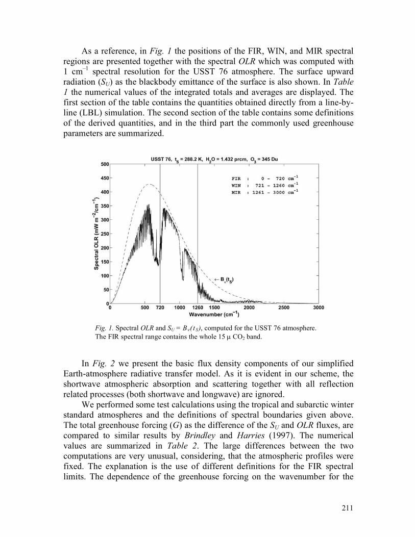
On a purely physical basis, one may set the FIR upper wave number limit before or after the CO2 15 µ fundamental absorption band. Although the separate treatment of the 15 µ CO2 band, (620–720 cm–1), is popular in broad band spectral radiative transfer models, to emphasize that the atmosphere is mostly opaque in the 1–720 cm–1 spectral region, in this work we have adopted the next definitions: total: 1–3000 cm–1; FIR: 1–720 cm–1; WIN: 720–1260 cm–1; MIR: 1260–3000 cm–1.

211

As a reference, in Fig. 1 the positions of the FIR, WIN, and MIR spectral regions are presented together with the spectral OLR which was computed with 1 cm–1 spectral resolution for the USST 76 atmosphere. The surface upward radiation (SU) as the blackbody emittance of the surface is also shown. In Table 1 the numerical values of the integrated totals and averages are displayed. The first section of the table contains the quantities obtained directly from a line-by-line (LBL) simulation. The second section of the table contains some definitions of the derived quantities, and in the third part the commonly used greenhouse parameters are summarized.

Fig. 1. Spectral OLR and SU = Bν(t S), computed for the USST 76 atmosphere. The FIR spectral range contains the whole 15 µ CO2 band.

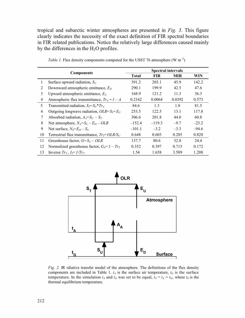
In Fig. 2 we present the basic flux density components of our simplified Earth-atmosphere radiative transfer model. As it is evident in our scheme, the shortwave atmospheric absorption and scattering together with all reflection related processes (both shortwave and longwave) are ignored.

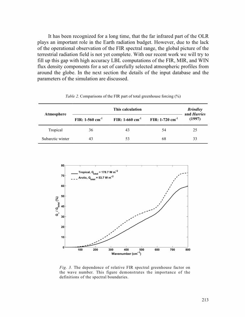
We performed some test calculations using the tropical and subarctic winter standard atmospheres and the definitions of spectral boundaries given above. The total greenhouse forcing (G) as the difference of the SU and OLR fluxes, are compared to similar results by Brindley and Harries (1997). The numerical values are summarized in Table 2. The large differences between the two computations are very unusual, considering, that the atmospheric profiles were fixed. The explanation is the use of different definitions for the FIR spectral limits. The dependence of the greenhouse forcing on the wavenumber for the

212

tropical and subarctic winter atmospheres are presented in Fig. 3. This figure clearly indicates the necessity of the exact definition of FIR spectral boundaries in FIR related publications. Notice the relatively large differences caused mainly by the differences in the H2O profiles.

Table 1. Flux density components computed for the USST 76 atmosphere (W m–2)

Spectral intervals Components

Total FIR MIR WIN 1 Surface upward radiation, SU 391.2 203.1 45.9 142.2 2 Downward atmospheric emittance, ED 290.1 199.9 42.5 47.6 3 Upward atmospheric emittance, EU 168.9 121.2 11.3 36.3 4 Atmospheric flux transmittance, TrA =1 – A 0.2162 0.0064 0.0392 0.573

5 Transmitted radiation, ST=SU*TrA 84.6 1.3 1.8 81.5 6 Outgoing longwave radiation, OLR=ST+EU 253.5 122.5 13.1 117.8 7 Absorbed radiation, AA=SU – ST 306.6 201.8 44.0 60.8 8 Net atmosphere, NA=SU – ED – OLR –152.4 –119.3 –9.7 –23.2 9 Net surface, NS=ED – SU –101.1 –3.2 –3.3 –94.6

10 Terrestrial flux transmittance, TrT=OLR/SU 0.648 0.603 0.285 0.828 11 Greenhouse factor, G=SU – OLR 137.7 80.6 32.8 24.4 12 Normalized greenhouse factor, GN=1 – TrT 0.352 0.397 0.715 0.172 13 Inverse TrT , IT=1/TrT 1.54 1.658 3.509 1.208

Fig. 2. IR rdiative transfer model of the atmosphere. The definitions of the flux density components are included in Table 1. tA is the surface air temperature, tG is the surface temperature. In the simulation tA and tG was set to be equal, tS = tA = tG, where tS is the thermal equilibrium temperature.

213

It has been recognized for a long time, that the far infrared part of the OLR

plays an important role in the Earth radiation budget. However, due to the lack of the operational observation of the FIR spectral range, the global picture of the terrestrial radiation field is not yet complete. With our recent work we will try to fill up this gap with high accuracy LBL computations of the FIR, MIR, and WIN flux density components for a set of carefully selected atmospheric profiles from around the globe. In the next section the details of the input database and the parameters of the simulation are discussed.

Table 2. Comparisons of the FIR part of total greenhouse forcing (%)

This calculation Atmosphere

FIR: 1-560 cm-1 FIR: 1-660 cm-1 FIR: 1-720 cm-1

Brindley and Harries

(1997)

Tropical 36 43 54 25

Subarctic winter 43 53 68 33

Fig. 3. The dependence of relative FIR spectral greenhouse factor on the wave number. This figure demonstrates the importance of the definitions of the spectral boundaries.

214

2. Global data set and LBL simulation Our qualitative estimates of the meridional distributions of the FIR, MIR, and WIN flux density components were based on a representative subset of the TIROS Initial Guess Retrieval (TIGR), global radiosonde archive (Chedin and Scott, 1983). From the TIGR archive, about 230 atmospheric profiles were extracted in a way that the temporal and spatial statistical characteristics of the original data set were preserved. The profiles were chosen regardless of the surface type. The surface emissivity was set to unity and the temperature of the emitting surface (tG) was set to the temperature of the lowest atmospheric level (tA): S A Gt t t= = , where tS is the common temperature. The global average surface temperature and water vapor column amount (w) are 285.3 K and 2.53 precipitable cm (prcm), respectively. Further on we shall use the term “global avareage” to indicate that the average value is computed from zonal mean values weighted with the cosine of the latitude. It is usually hard to tell how representative a data set for global and annual climatology research is. We believe, that our data set contains sufficient information to characterize the contributions of different spectral ranges to the meridional distributions of the total and spectral clear-sky flux density components. Here we note, that the temperature profile set represents real equilibrium situations, where all kind of energy sources and sinks in the layered atmosphere are balanced by IR radiative cooling or heating. More details on the profile selection strategy can be found in Miskolczi and Rizzi (1998).

For the radiative transfer computations we used the High-resolution Atmospheric Radiative Transfer Code (HARTCODE), (Miskolczi et al., 1990). More results on the validation of HARTCODE may be found in Rizzi et al. (2002) and Kratz et al. (2005). Here we shall not go into the full details of an LBL simulation, but summarize only a few important basic features. This work partly uses the results of a previous study performed to evaluate the temperature and water vapor sounding capabilities of the Advanced Earth Observing Satellite (ADEOS2) Global Imager (GLI) instrument, and therefore, particulars of the LBL simulations were already reported in Miskolczi and Rizzi (1998).

A large data set of directional radiances and transmittances computed for the TIGR profiles and GLI spectral range, (800–2800 cm–1), with 1.0 cm–1 spectral resolution were already available. To obtain the total flux densities, additional radiance computations were done for the spectral ranges not covered by the GLI instrument. The directional radiances were determined in nine streams, and assuming cylindrical symmetry, a simple code was developed to facilitate the integration over the solid angle.

215

For the spectral range covered by the GLI instrument the GEISA (Husson et al., 1994), absorption line compilation were used and for the remaining part of the spectra we used the HITRAN2K line catalog (Rothman et al., 1998; HITRAN2K, 2002).

The atmosphere was stratified using 32 exponentially placed layers with about 100 m and 10 km layer thickness at the bottom and the top, respectively. The full altitude range was set to 61 km and the slant path was determined by spherical refractive geometry. The upward and downward slant path were identical, which assured that the directional spectral transmittances for the reverse trajectories were equal. Altogether eleven absorbing molecular species were involved: H2O, CO2, O3, N2O, CH4, NO, SO2, NO2, CCl4, F11, and F12.

The H2O continuum absorption parameterization was similar to the CKD2.4 without the slight recent adjustments made in some part of the far infrared range (Tobin et al., 1999). In the most affected spectral ranges of the CO2 Q bands, the line-mixing effects were considered using a recent line-mixing parameterization by Rodriguez et al. (1999). No adjustments were implemented for the non-local thermodynamic effects and the effects of the aerosols were also ignored.

The direct output from HARTCODE were the spectral atmospheric upward emittance ( ,UEν ), downward emittance ( ,DEν ), surface upward flux density ( ,USν ), and the atmospheric flux transmittance ( ,ATrν ). The atmospheric spectral flux transmittance, by definition, is the ratio of the transmitted flux density ( ,TSν ) to the surface upward flux density: , , ,1 /A T UTr A S Sν ν ν ν= − = , where Aν is the spectral flux absorptance. The spectral outgoing longwave radiation is taken as the sum of the transmitted flux density and atmospheric upward emittance, , ,T UOLR S Eν ν ν= + . The spectrally integrated and/or averaged quantities are indicated by omitting the subscript ν. The definitions of other derived quantities are given in Fig. 2 and Table 1.

The ratio of the OLR to the surface upward flux density is sometimes called flux transmittance or total flux transmittance (TrT). To distinguish this quantity from the atmospheric flux transmittance, further on we shall call this quantity terrestrial flux transmittance: TrT= OLR/SU. We use the term “total” to indicate integration over the 1–3000 cm–1 spectral range. In Table 3 we present the basic statistics and global averages of the computed

, , ,U D TS E OLR S , and G parameters. Throughout this paper we frequently refer to figures with one or more

parameterized functions. To make the reference to those parameterized functions easier, we supplied their serial number with a prefix character (#) and included them into Table 4. When referencing to them only their special serial numbers are quoted.

216

Table 3. Basic statistics and global averages of the flux density components (W m-2)

Spectral regions Parameters SU ED OLR ST G

Minimum 165 103 150 22 5.9

Maximum 521 429 297 112 223

Mean 313 235 223 69 89 Std. 82 82 34 13 49

Total

Global 382 309 250 61 132

Minimum 112 89 100 0.0 4.2

Maximum 244 241 140 29 120

Mean 173 166 119 7.0 54 Std. 31 37 8.0 7.2 25

FIR

Global 199 195 123 2.6 75

Minimum 7.4 6.6 6.0 0.7 0.4

Maximum 79 73 21 2.8 63

Mean 31 29 11 1.4 20 Std. 16 16 3.0 0.3 14

MIR

Global 45 43 14 1.3 31

Minimum 46 8.0 44 21 1.3

Maximum 198 139 157 108 47

Mean 109 40 93 61 16 Std. 35 32 25 13 11

WIN

Global 138 71 113 57 25

3. Results and discussion 3.1 Outgoing logwave radiation

One may not expect that a limited data set of 230 profiles will reproduce accurately the detailed meridional picture, especially around the highly variable ITC zone. However, it is possible to characterize the average behavior and tendency of the meridional variation by the zonal means or by a smooth curve – usually a low order polynomial or spline – fitted to the zonal means. This is clearly demonstrated in Fig. 4, where the simulated zonal mean OLR from the

217

Table 4. Parameterized functions in the Figures, (u=ln(w))

Fig. X Y Curve FUNCTION Y = f(X) r No.

Total exp(-1.461 - 0.2819 x - (1231 x2 + 541.9 x3 + 84.66 x4)/104) 0.993 #1

FIR exp(-4.292 - 2.255 x – 0.8324 x2 – 0.1781 x3 - 0.01521 x4) 0.998 #2

MIR exp(-3.190-0.5659 x + 0.02778 x2 + 0.01022 x3 -0.0007153x4) 0.998 #3 7 u TrA

WIN exp(-0.2249 – 0.2543 x + 0.01545 x2 - 0.007840 x3 + 0.0007537x4) 0.994 #4

Total exp(0.3833 + 0.1908 x + 0.05183 x2 + 0.01988 x3 + 0.002399 x4) 0.992 #5

FIR exp(1.45+0.523x+(744 x2-43.1x3–86.2x4 -19.14x5-0.776x6)/104) 0.996 #6 u

MIR exp(1.161+0.1765x-0.02598 x2 + 0.0004931 x3 + 0.0008610 x4) 0.997 #7 8

w

τA

WIN 0.2214 + 0.2611 x 0.992 #8

Total exp(-1.098 + 0.3055 x) 0.896 #9

FIR exp(-0.9682 + 0.3 x) 0.884 #10

MIR exp(-0.009824 + 0.2281 x) 0.834 #11 9 u τT

WIN exp(-1.912 + 0.3473 x) 0.903 #12

10 TrF TrT 0.09922 + 0.9043 x 0.997 #13

Total 0.4961 + 0.0009681 x 0.028 #14 w

FIR 0.7026-.04167 x + 0.002596 x2 0.658 #15

u MIR exp(-1.1101 - 0.216 x) 0.738 #16 14

w

RU

WIN 0.1311 + 0.1276 x - 0.008184 x2 0.975 #17

u Total 0.7371 + 0.06411 x + 0.0156 x2 + 0.003123 x3 0.947 #18

FIR 1 - 0.52071 exp(-3.213 x0.4555) 0.965 #19

MIR 1 - 0.6766 exp(-2.293 x0.1656) 0.842 #20 17

w RD

WIN -1.518 + 1.67 exp(0.09220 x -0.006403 x2) 0.987 #21

Total 22.32 + 7.921 x + 0.86 x2 0.913 #22

FIR 11.59 + 3.177 x + 0.22 x2 0.892 #23

MIR 1.163 + 0.4868 x + 0.06251 x2 0.931 #24 dtG

WIN 9.566 + 4.256 x + 0.5768 x2 0.917 #25

30 u

dtE Total 23.46 + 7.376 x + 0.6058 x2 0.886 #26

Total 17.43 - 4.552 x - 1.178 x2 - 0.1971 x3 + 0.02624 x4 0.982 #27 u

FIR 12.28 - 4.614 x - 0.6769 x2 - 0.01734 x3 + 0.03412 x4 0.994 #28

MIR 2.023 + 0.2647 -.1893 x + 0.01746 x2 0.727 #29 w

dtA

WIN 2.254 + 1.089 - 0.3753 x + 0.02855 x2 0.795 #30

32

dtA tS Total 302.7 - 0.08994 x - 0.08778 x2 0.869 #31 The correlation coefficient is defined as: r = (1-σ2

R /σ2Y)0.5, where σR is the residuum standard deviation.

218

TIGR data set are compared to the mean clear-sky and all-sky meridional distributions obtained from the ERBE measurements. The top and bottom curves in this plot were obtained by fitting a third order polynomial to the zonal averages of about 70,000 all-sky and 40,000 clear-sky annual average OLR measurements from the ERBS, NOAA9, and NOAA10 satellites. The markers in this figure are the TIGR OLR fluxes averaged over latitudinal belts of 5-degree widths.

Fig. 4. Computed and measured OLR. The dotted and dashed curves are third order polynomials fitted to the ERBE clear-sky and ERBE all-sky zonal mean data points (ERBE, 2004).

The total OLR curve from the TIGR data set is between the clear-sky and

all-sky OLR curves from the ERBE, and the shape of the curves are very similar. Considering the surface temperature and emissivity settings in this simulation, this figure shows a remarkable agreement with the ERBE data set. The global averages of the OLRs are 250, 268, and 236 W m–2 for this simulation, the ERBE clear-sky and ERBE all-sky cases, respectively. Fig. 5 shows the spectral decomposition of the OLR. The decreasing total OLR toward the poles are mainly due to the reduced upward fluxes in the WIN region.

To a somewhat lesser extent, the FIR and MIR spectral regions also contribute to the poleward reduction of the total OLR. This is an indication of the presence of relatively small amounts of transmitted surface fluxes. Compared to the total OLR, the poleward variation in the FIR part is surprisingly small, not exceeding 5–7%.

219

Fig. 5. Latitudinal distributions of the total and spectral components of the outgoing longwave radiation. The FIR and MIR components have very small latitudinal variation. The short vertical ‘bars’ are the estimated five year average ERBE FIR OLR.

The total OLR contains the FIR OLR and, therefore, theoretically there

should be a strong correlation between the two quantities. According to our data set, a linear relationship exists between the total and FIR OLR with a 0.88 correlation coefficient. Utilizing this relationship, we estimated the FIR component of the ERBE clear-sky OLR, and plotted it in Fig. 5 as dots. In the plot, due to the large number of data points, the dots are organized into short vertical “bars”. The vertical extensions of the bars indicate the variability of the ERBE FIR OLRs at a given latitude. The distances between the bars are 2.5 degrees, corresponding to the latitudinal resolution of the ERBE archive. Since it is known a-priori, that the surface and atmospheric temperatures are significantly decreasing poleward, the more or less constant meridional TIGR and ERBE FIR OLR must be the result of a delicate compensation mechanism. The interesting question is how the surface temperature, temperature, and humidity profiles, and the atmospheric spectral transparency are linked together to produce the above phenomenon. 3.2 Flux transmittance and graybody optical thickness The atmospheric transparency is increasing with decreasing absorber amount. In the Earth’s atmosphere water vapor is the major absorber, therefore, the meridional distribution of TrA must obey the poleward decrease of the water vapor column amount. As it is evident from Fig. 6, the total, MIR, and WIN

220

Fig. 6. Latitudinal distributions of the total and spectral components of the atmospheric flux transmittance, TrA=ST/SU .

Fig. 7. Dependence of total and spectral atmospheric flux transmittance components on water vapor column amount. The large dots are the parameterized WIN TrA functios tested with an independent set of eight profiles.

221

components of TrA are increasing poleward, while the FIR part is effectively zero in the equatorial regions, reaching only 10% at the poles. The MIR TrA behaves similarly,except, it is always larger than zero because of the presence of larger transparent regions within the MIR spectral range.

In Fig. 7 the total and spectral components of the TrA are plotted as the function of w. The small dots are for the total TrA. The parametrization of TrA with the water vapor column amount is of common interest. Eqs. #1–#4 are the appropriate functions that reproduce TrA with a residuum correlation coefficient better than 0.995 . The validity of Eq. #4 was tested with an independent profile set consisting of five climatological average profiles, the USST 76 atmosphere, and two extreme TIGR profiles. The computed window transmittances are marked by larger dots. Obviously, Eq. (4) is valid for the full range of w in the Earth’s atmosphere.

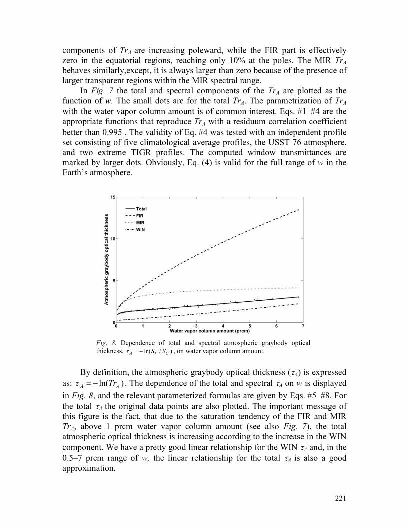
Fig. 8. Dependence of total and spectral atmospheric graybody optical thickness, ln( / )A T US Sτ = − , on water vapor column amount.

By definition, the atmospheric graybody optical thickness (τA) is expressed

as: ln( )A ATrτ = − . The dependence of the total and spectral τA on w is displayed in Fig. 8, and the relevant parameterized formulas are given by Eqs. #5–#8. For the total τA the original data points are also plotted. The important message of this figure is the fact, that due to the saturation tendency of the FIR and MIR TrA, above 1 prcm water vapor column amount (see also Fig. 7), the total atmospheric optical thickness is increasing according to the increase in the WIN component. We have a pretty good linear relationship for the WIN τA and, in the 0.5–7 prcm range of w, the linear relationship for the total τA is also a good approximation.

222

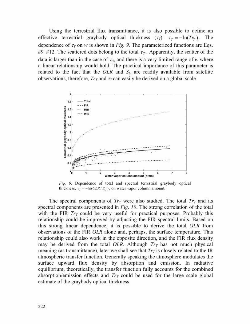
Using the terrestrial flux transmittance, it is also possible to define an effective terrestrial graybody optical thickness (τT): ln( )T TTrτ = − . The dependence of τT on w is shown in Fig. 9. The parameterized functions are Eqs. #9–#12. The scattered dots belong to the total Tτ . Apparently, the scatter of the data is larger than in the case of τA, and there is a very limited range of w where a linear relationship would hold. The practical importance of this parameter is related to the fact that the OLR and SU are readily available from satellite observations, therefore, TrT and τT can easily be derived on a global scale.

Fig. 9. Dependence of total and spectral terrestrial graybody optical thickness, ln( / )T UOLR Sτ = − , on water vapor column amount.

The spectral components of TrT were also studied. The total TrT and its

spectral components are presented in Fig. 10. The strong correlation of the total with the FIR TrT could be very useful for practical purposes. Probably this relationship could be improved by adjusting the FIR spectral limits. Based on this strong linear dependence, it is possible to derive the total OLR from observations of the FIR OLR alone and, perhaps, the surface temperature. This relationship could also work in the opposite direction, and the FIR flux density may be derived from the total OLR. Although TrT has not much physical meaning (as transmittance), later we shall see that TrT is closely related to the IR atmospheric transfer function. Generally speaking the atmosphere modulates the surface upward flux density by absorption and emission. In radiative equilibrium, theoretically, the transfer function fully accounts for the combined absorption/emission effects and TrT could be used for the large scale global estimate of the graybody optical thickness.

223

Fig. 10. Terrestrial total flux transmittance and its spectral components. The relatively larger scatter of the MIR and WIN data points are indication of increased ST in those spectral ranges.

3.3 Transmitted surface radiation and atmospheric emittance

While the OLR can easily be measured with sufficient accuracy by satellite radiometers, the transmitted flux density and the upward atmospheric emittance can only be derived by lengthy computations of the accurate spectral flux transmittance.

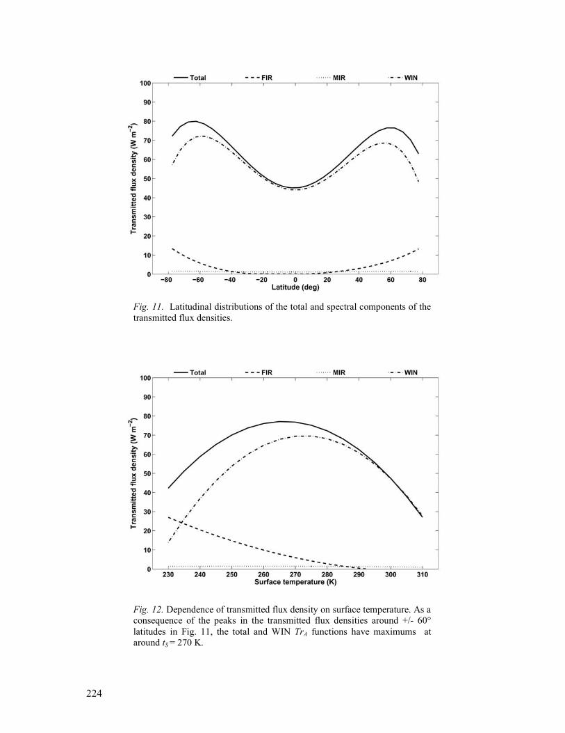
The transmitted spectral flux density from the surface and the atmospheric upward emissivity may be written as ST = SUTrA and EU=OLR – ST, respectively. The meridional distribution of the total ST and its spectral components are presented in Fig. 11. It is not a surprise that the total ST is governed by the WIN component, however, the latitudinal distribution of the WIN and the total ST is very interesting. From the equatorial regions to about +/– 60° latitudes, ST is increasing despite the large poleward decrease in the surface temperature. Proceeding toward the arctic regions, ST will drop again considerably. The explanation for this unique behavior lies in the relative rate of the poleward decrease of the surface temperature and poleward increase of atmospheric transparency. After about +/– 60° latitudes, the temperature decrease will be the dominant factor.

This latitudinal dependence of ST has an implication on its temperature dependence. Namely, the transmitted surface radiation is not increasing monotonously with the surface temperature, but must have a maximum value at around 270 K, representing the +/– 60° latitudes, see Fig. 12. Further on, this also implies that from +/– 60° latitudes toward the equator the surface net

224

Fig. 11. Latitudinal distributions of the total and spectral components of the transmitted flux densities.

Fig. 12. Dependence of transmitted flux density on surface temperature. As a consequence of the peaks in the transmitted flux densities around +/- 60° latitudes in Fig. 11, the total and WIN TrA functions have maximums at around tS = 270 K.

225

radiation (atmospheric downward minus surface upward) will increase with increasing tS. The above phenomenon is called “super-greenhouse effect” (Vonder Haar, 1986), and it is controlled by the strong H2O continuum absorption in the windows region and the meridional distributions of w. At the polar regions or beyond +/– 60° latitudes, the longwave total net surface flux density is decreasing with increasing tS, meaning, that the rate of warming of the surface by the downward atmospheric emittance is less efficient than the rate of energy loss of the surface.

In Fig. 11 the FIR component has a steady rise toward the poles from about +/– 20–30° latitudes. The little asymmetry in the region of the total absorption around the equator is related to the asymmetry in the latitudinal distribution of w. The contribution to the total ST from the MIR spectral range is not significant (1–2 W m–2) and does not change much along the latitudes.

The latitudinal variation of the FIR and WIN EU are displayed together with the FIR and WIN OLR in Fig. 13. The FIR OLR is largely made up by the FIR EU. In the polar regions the transmitted surface flux contributions may reach 15–20%. The WIN EU contributions to the WIN OLR is decreasing poleward, up to +/– 65° latitudes. At higher latitudes there is a small increase in the WIN EU, which could be the consequence of relatively higher temperatures in the lower troposphere due to frequent temperature profile inversions.

Fig. 13. Latitudinal distributions of the total, FIR and WIN OLR and the FIR and WIN upward atmospheric emittance.

226

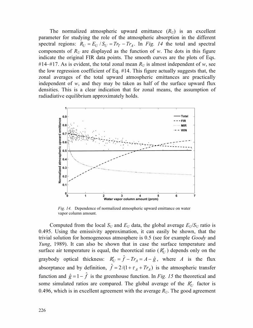
The normalized atmospheric upward emittance (RU) is an excellent parameter for studying the role of the atmospheric absorption in the different spectral regions: /U U U T AR E S Tr Tr= = − . In Fig. 14 the total and spectral components of RU are displayed as the function of w. The dots in this figure indicate the original FIR data points. The smooth curves are the plots of Eqs. #14–#17. As is evident, the total zonal mean RU is almost independent of w, see the low regression coefficient of Eq. #14. This figure actually suggests that, the zonal averages of the total upward atmospheric emittances are practically independent of w, and they may be taken as half of the surface upward flux densities. This is a clear indication that for zonal means, the assumption of radiadiative equilibrium approximately holds.

Fig. 14. Dependence of normalized atmospheric upward emittance on water vapor column amount.

Computed from the local SU and EU data, the global average EU/SU ratio is

0.495. Using the emissivity approximation, it can easily be shown, that the trivial solution for homogeneous atmosphere is 0.5 (see for example Goody and Yung, 1989). It can also be shown that in case the surface temperature and surface air temperature is equal, the theoretical ratio ( UR′ ) depends only on the graybody optical thickness: ˆ ˆU AR f Tr A g′ = − = − , where A is the flux absorptance and by definition, ˆ 2 /(1 )A Af Trτ= + + is the atmospheric transfer function and ˆˆ 1g f= − is the greenhouse function. In Fig. 15 the theoretical and some simulated ratios are compared. The global average of the UR′ factor is 0.496, which is in excellent agreement with the average RU. The good agreement

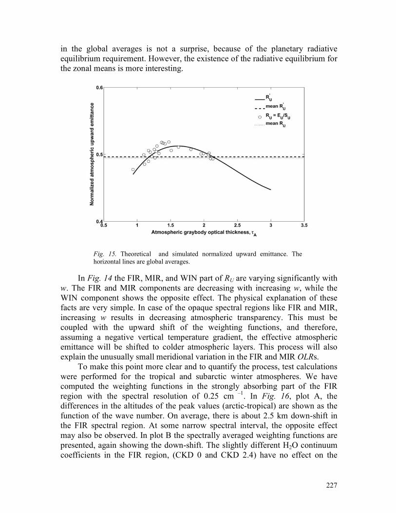
227

in the global averages is not a surprise, because of the planetary radiative equilibrium requirement. However, the existence of the radiative equilibrium for the zonal means is more interesting.

Fig. 15. Theoretical and simulated normalized upward emittance. The horizontal lines are global averages.

In Fig. 14 the FIR, MIR, and WIN part of RU are varying significantly with w. The FIR and MIR components are decreasing with increasing w, while the WIN component shows the opposite effect. The physical explanation of these facts are very simple. In case of the opaque spectral regions like FIR and MIR, increasing w results in decreasing atmospheric transparency. This must be coupled with the upward shift of the weighting functions, and therefore, assuming a negative vertical temperature gradient, the effective atmospheric emittance will be shifted to colder atmospheric layers. This process will also explain the unusually small meridional variation in the FIR and MIR OLRs.

To make this point more clear and to quantify the process, test calculations were performed for the tropical and subarctic winter atmospheres. We have computed the weighting functions in the strongly absorbing part of the FIR region with the spectral resolution of 0.25 cm –1. In Fig. 16, plot A, the differences in the altitudes of the peak values (arctic-tropical) are shown as the function of the wave number. On average, there is about 2.5 km down-shift in the FIR spectral region. At some narrow spectral interval, the opposite effect may also be observed. In plot B the spectrally averaged weighting functions are presented, again showing the down-shift. The slightly different H2O continuum coefficients in the FIR region, (CKD 0 and CKD 2.4) have no effect on the

228

conclusions of the qualitative picture. The average peak positions were moving from about 7.7 km, in the case of the tropical atmosphere to about 5.2 km in the case of the arctic winter atmosphere. Apparently, the peaks are always above a possible low level inversion and below the stratospheric temperature rise, even if we consider the lowering of the height of the tropopause toward the poles.

Fig. 16. Relative position of the peak of the FIR spectral weighting functions, (plot A), and the average FIR weighting functions, (plot B). Note the relatively small effect of the changes in the H2O continuum parameterization in plot B.

The thermal structure of the atmosphere between the 5 and 10 km altitude

range or up to the tropopause is usually characterized with a negative temperature gradient explaining the increasing FIR and MIR RU with decreasing w (in Fig. 14). As an indirect evidence of the above process, by the simulation of the response of the OLR of the arctic winter atmosphere to the decrease in the H2O continuum absorption coefficient in the FIR spectral range, it was shown in Tobin et al. (1999) that the top of the atmosphere flux density increases.

The explanation of the behavior of the WIN RU is also simple. Since the whole vertical atmosphere contributes to the EU, its increasing value with increasing w indicates, that larger w is usually associated with warmer atmosphere, and the fractional amount of the upward re-emitted radiation is roughly proportional to the absorbed radiation. The WIN TrT does not change very much; the global average is 0.8544 and the standard deviation is about 6%. Consequently, the relationship ~ 0.8544U AR Tr− means, that the relative upward atmospheric windows emittance depends only on the total absorption.

229

Just for completeness, in Fig. 17 the total and spectral normalized atmospheric downward emittances (RD) are presented as the function of w , see also Eqs. #18–#21. RD is computed similarly to RU, but using the atmospheric downward emittance : /D D UR E S= . According to the Kirchoff’s law, RD may be identified as the clear-sky total graybody absorptance: 1D AR Tr A= − = . For the recent TIGR profile set – which contains some very cold and dry as well as very warm and humid profiles – RD varies between 0.63 and 0.93. The only interesting feature of this figure is the saturation of the FIR RD at around 2 prcm water vapor column amount. The sharp decrease in RD with decreasing water vapor content is the result of the opening up of the so called “micro windows” in the FIR spectral region as it was also evidenced by the Surface Heat Budget of the Arctic Ocean, SHEBA, experiment (Tobin et al., 1999). The FIR and MIR RD may exceed one, which is the indication of cases with strong close to surface temperature profile inversions. The total RD may be parameterized with quite a high accuracy using a third order polynomial of u, Eq. (18): ( )DR f u′ = , where

ln( )u w= .

Fig. 17. Dependence of normalized atmospheric downward emittance on water vapor column amount.

ED is an important term in the equation of the surface energy balance, and

lots of efforts were devoted for its parameterization (Brutsaert, 1975; Idso, 1981; Tuzet, 1990). Using satellite observations of the air temperature at the surface and the water vapor column amount, together with the parameterized value of the clear-sky RD by Eq. #18, the estimated downward emittance ( )DE′

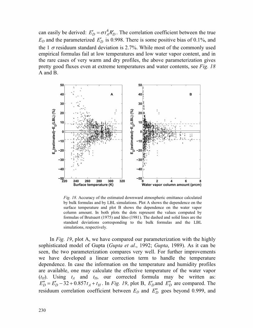
230

can easily be derived: 4D A DE t Rσ′ ′= . The correlation coefficient between the true

ED and the parameterized DE′ is 0.998. There is some positive bias of 0.1%, and the 1 σ residuum standard deviation is 2.7%. While most of the commonly used empirical formulas fail at low temperatures and low water vapor content, and in the rare cases of very warm and dry profiles, the above parameterization gives pretty good fluxes even at extreme temperatures and water contents, see Fig. 18 A and B.

Fig. 18. Accuracy of the estimated downward atmospheric emittance calculated by bulk formulas and by LBL simulations. Plot A shows the dependence on the surface temperature and plot B shows the dependence on the water vapor column amount. In both plots the dots represent the values computed by formulas of Brutsaert (1975) and Idso (1981). The dashed and solid lines are the standard deviations corresponding to the bulk formulas and the LBL simulations, respectively.

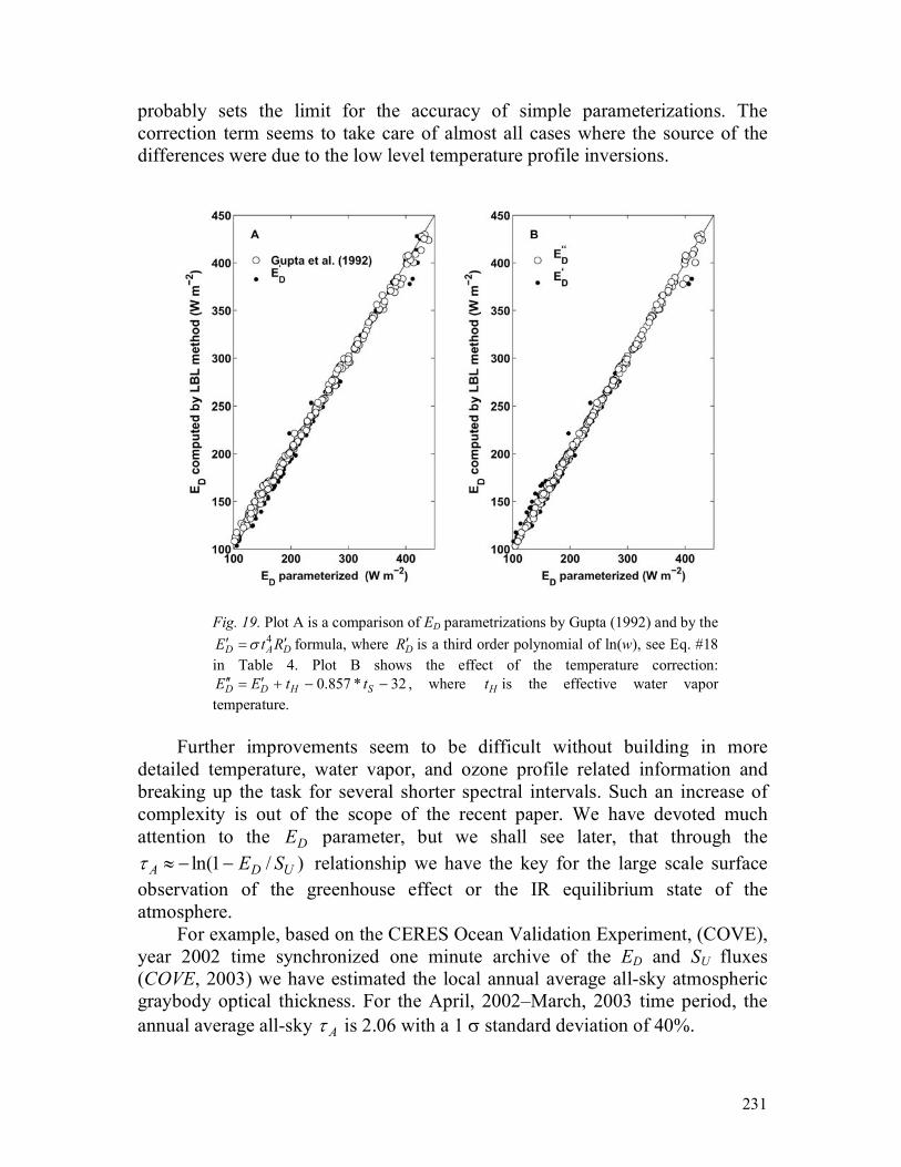
In Fig. 19, plot A, we have compared our parameterization with the highly

sophisticated model of Gupta (Gupta et al., 1992; Gupta, 1989). As it can be seen, the two parameterization compares very well. For further improvements we have developed a linear correction term to handle the temperature dependence. In case the information on the temperature and humidity profiles are available, one may calculate the effective temperature of the water vapor (tH). Using tA and tH, our corrected formula may be written as:

32 0.857D D A HE E t t′′ ′= − + + . In Fig. 19, plot B, DE′ and DE′′ are compared. The residuum correlation coefficient between ED and DE′′ goes beyond 0.999, and

231

probably sets the limit for the accuracy of simple parameterizations. The correction term seems to take care of almost all cases where the source of the differences were due to the low level temperature profile inversions.

Fig. 19. Plot A is a comparison of ED parametrizations by Gupta (1992) and by the 4

D A DE t Rσ′ ′= formula, where DR′ is a third order polynomial of ln(w), see Eq. #18 in Table 4. Plot B shows the effect of the temperature correction:

0.857 * 32D D H SE E t t′′ ′= + − − , where Ht is the effective water vapor temperature.

Further improvements seem to be difficult without building in more

detailed temperature, water vapor, and ozone profile related information and breaking up the task for several shorter spectral intervals. Such an increase of complexity is out of the scope of the recent paper. We have devoted much attention to the DE parameter, but we shall see later, that through the

ln(1 / )A D UE Sτ ≈ − − relationship we have the key for the large scale surface observation of the greenhouse effect or the IR equilibrium state of the atmosphere.

For example, based on the CERES Ocean Validation Experiment, (COVE), year 2002 time synchronized one minute archive of the ED and SU fluxes (COVE, 2003) we have estimated the local annual average all-sky atmospheric graybody optical thickness. For the April, 2002–March, 2003 time period, the annual average all-sky Aτ is 2.06 with a 1 σ standard deviation of 40%.

232

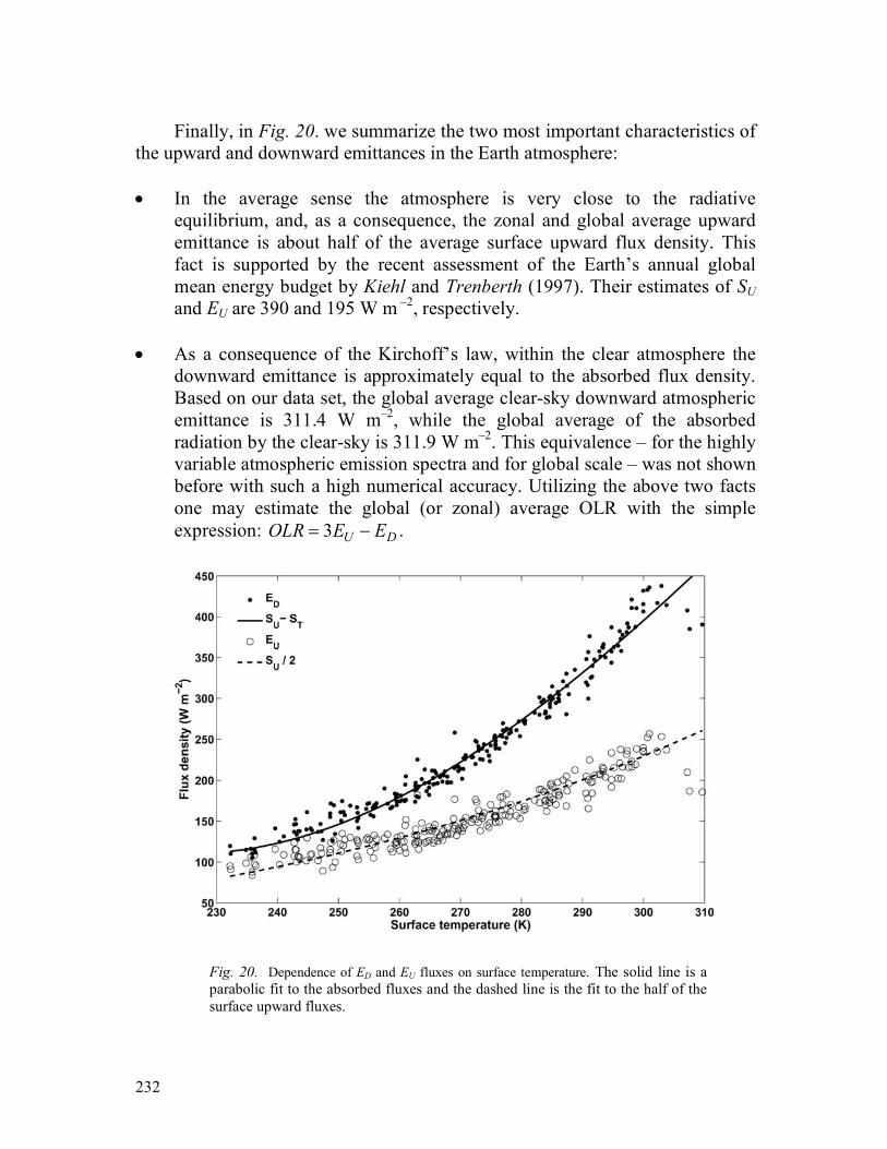
Finally, in Fig. 20. we summarize the two most important characteristics of

the upward and downward emittances in the Earth atmosphere:

• In the average sense the atmosphere is very close to the radiative equilibrium, and, as a consequence, the zonal and global average upward emittance is about half of the average surface upward flux density. This fact is supported by the recent assessment of the Earth’s annual global mean energy budget by Kiehl and Trenberth (1997). Their estimates of SU and EU are 390 and 195 W m –2, respectively.

• As a consequence of the Kirchoff’s law, within the clear atmosphere the

downward emittance is approximately equal to the absorbed flux density. Based on our data set, the global average clear-sky downward atmospheric emittance is 311.4 W m–2, while the global average of the absorbed radiation by the clear-sky is 311.9 W m–2. This equivalence – for the highly variable atmospheric emission spectra and for global scale – was not shown before with such a high numerical accuracy. Utilizing the above two facts one may estimate the global (or zonal) average OLR with the simple expression: 3 U DOLR E E= − .

Fig. 20. Dependence of ED and EU fluxes on surface temperature. The solid line is a parabolic fit to the absorbed fluxes and the dashed line is the fit to the half of the surface upward fluxes.

233

4. Greenhouse effect 4.1 Overview Regarding the planetary greenhouse effect we must relate the amount of the atmospheric absorbers to the surface temperature. Assuming monochromatic radiative equilibrium, isotropy in both hemispheres and a semi-infinite plane-parallel gray atmosphere, the predicted air temperature at the surface ( At′ ) and the surface temperature ( Gt′ ) are given by the next two equations (Goody and Yung, 1989; Paltridge and Platt, 1976):

14(1 )

2A AOLRt τσ

′ = + , (1)

and 14(2 )

2G AOLRt τσ

′ = + . (2)

In the above equations Aτ is the total graybody atmospheric optical

thickness, as usually defined in two stream approximations, (3/ 2)Aτ τ= , where τ is measured vertically. The atmospheric skin temperature ( 0t′ ) and the characteristic graybody optical thickness which defines the IR optical surface of the planet ( Cτ ′ ) are:

0

14

2OLRtσ

′ = , (3)

1Cτ ′ = . (4)

Eqs. (1)–(4) are usually referred as the solutions of the Schwarzschild-Milne equations, see more details in Rozanov (2001), Rutten (2000), or in Collins II, (2003). We should note, that the terrestrial graybody optical thickness is not an accurate measure of the atmospheric absorption and can not be used in Eqs. (1) and (2). These equations are frequently quoted in the meteorological literature and even in textbooks, however, it is a mistake to use them to study the radiative equilibrium and greenhouse effect in the Earth’s atmosphere.

For the real atmosphere, the semi-infinite solutions must be replaced with the solutions valid for the bounded atmosphere. With relatively simple

234

computation (we do not present it here) it can be shown, that for a given OLR or EU the surface air temperature and surface temperature are mutually dependent on each other: ˆ ( )A G AOLR f S A S Tr= + or ˆ ˆU A G AE f S A gS Tr= − , where SG and SA are the surface upward flux densities at tG and tA temperatures, respectively. The IR atmospheric transfer and the greenhouse functions ( f and g ) play fundamental role in the planetary greenhouse effect.

In our simulation, for having no surface temperature data, and making the definition of the greenhouse effect simpler, we set the equilibrium surface temperatures to the surface air temperatures, G A St t t= = . Note, that in the boundary layer the principle of energy minimum (or maximum entropy) works toward the thermal equilibrium. In this case the theoretical dependence of St on the transfer function f is:

114(1 )4

ˆ 2

AA

SOLR OLR et

f

ττσσ

− + + ′′ = =

. (5)

In case the lower boundary condition is explicitly set by tG, the atmospheric

skin temperature will also depend on the surface temperature and total optical thickness:

0

14 4(1 (1 )) 2

2 (1 )

A AA G

A

OLR e e tte

τ ττ στσ

− − + + − ′′ =− −

. (6)

In Figs. 21 and 22 we compare the surface air and surface temperatures

obtained by the different formulas. For reference, in Fig. 21 the effective temperatures, 0.25( / )Et OLR σ= , and the atmospheric skin temperatures are also plotted. Apparently, At′ underestimates and Gt′ badly overestimates the corresponding equilibrium surface and surface air temperatures. The error in At′ decreases with increasing temperatures because of the increasing w (at higher temperatures). The atmospheric skin temperatures are also underestimated, and for the same reason the errors decrease with increasing temperatures.

The data points in these figures represent only about 10% of the total 230 profiles. Only those cases were selected for these plots, where the simulated and theoretically predicted OLRs agreed within less than 0.5%. Note, that (according to Fig. 14), for the zonal and global averages the radiative equilibrium condition

235

Fig. 21. Surface air, skin and effective temperatures predicted by Eqs. 1,3 , 5 and 6. The dotted line is the effective temperature, 0.25( / )Et OLR σ= . The symbols represent selected profiles with OLRs closest to the theoretical values.

Fig. 22. Surface temperatures predicted by Eqs. 2 and 5. The symbols represent selected profiles with OLRs closest to the theoretical values.

236

holds, but the individual profiles could be quite far from the radiative equilibrium. For example, it is obvious that profiles with temperature inversions will not fit into the theoretical picture which expects increasing temperatures with increasing optical thickness.

In the bounded atmosphere the characteristic graybody optical thickness ( Cτ ′′ ) becomes also dependent on the total optical thickness and surface temperature:

42 1

11

SA

CA

tOLR

e

στ

τ τ

− − ′′ = −

−. (7)

In Fig. 23 the Cτ ′′ and the simulated and theoretical atmospheric clear-sky graybody optical thicknesses are shown as the function of the surface temperature.

Fig. 23. Dependence of simulated and theoretical graybody optical thickness on surface temperature. The dash-dot line is the theoretical characteristic optical thickness, Cτ ′′ , computed by Eq. 7.

The theoretical values ( Aτ ′′ ) are the solutions of the transcendent equation for Aτ on the left hand side of Eq. (5). The Aτ ′′ and Aτ curves show excess optical thickness (water vapor) at very cold (arctic) and very warm (tropical) areas, while, there are optical thickness deficits at medium surface temperatures. With

237

increasing temperature – or w –, Cτ ′′ tends toward the semi-infinite solution of 1.0. Sometimes Cτ ′′ is associated with an atmospheric altitude or pressure level of effective emission, see for example Schneider et al. (1999). Since part of the OLR is, in fact, transmitted flux density from the surface, the physical meaning of such an atmospheric level is confusing. According to Schneider et al. (1999), the effective pressure level is between 540 and 600 hPa. Our computation shows a global average effective pressure level of 507 hPa. The global average effective pressure levels for the upward and downward atmospheric emissions are 339 and 666 hPa, subsequently.

The theoretical and simulated global average graybody optical thicknesses are in pretty good agreement: they are 1.87 and 1.86, and they correspond to a vertical optical thickness of about 1.23τ = . These values are also the indication that the clear atmosphere loses its thermal energy close to the peak efficiency, see Fig. 15. Using Eq. (1) with the same data would result in about 9% higher optical thickness, and using Eq. (2) would result in an unrealistic low value of 0.67. Just for reference, if we use a global average surface and surface air temperature of 288 K and the ERBE global average clear-sky OLR of 268.0 W m–2, the theoretically estimated vertical optical thickness would be 1.17, which is reasonably close to our global clear-sky average. The atmospheric greenhouse effect is bounded to the absorption and emission of the IR radiation and controlled by the IR atmospheric graybody optical thickness. The keys to this parameter are the accurate (measured or modeled) atmospheric upward and downward flux densities, the correct computation of the atmospheric flux transmittances, and an adequate radiative transfer model which relates the fluxes and flux transmittances. In the next section we shall shortly review the most commonly used greenhouse parameters and their relation to the atmospheric graybody optical thickness. 4.2 Greenhouse factor and normalized greenhouse factor The most common measure of the greenhouse effect, which is also adopted by the global warming community, is the difference between the SU and the OLR: G = SU – OLR (Raval and Ramanathan, 1989). The classical approach to the greenhouse effect is via the long-term energy balance equation of the solar radiation input and the IR radiation loss of the Earth surface. The difference between the effective planetary temperature – computed from the OLR or the solar input – and the global average surface temperature is the measure of the planetary greenhouse effect. In fact, the G factor is the application of the classical approach for the local flux densities without converting them to temperature differences. As we have seen in Fig. 20, the atmospheric absorption and the downward atmospheric emittance are approximately equal, therefore, the G factor can easily be related to the atmospheric upward and downward

238

emittances: (1 )U A U D UG S Tr E E E= − − = − . In case the surface air temperature and the surface temperature are equal, theoretically, the G factor is proportional to the product of US and the greenhouse function, which is only dependent on

Aτ : ˆ( , ) ( )U A U AG G S S gτ τ= = . The ˆ ( )Ag τ function may be expressed as:

1ˆ ( )1

AA

AA

A

ege

τττ ττ

−− +=

−+ +. (8)

Eq. (8) shows the real physical meaning of the / Ug G S= factor in Raval and Ramanathan (1989). The normalized greenhouse factor and the total atmospheric graybody optical thickness are uniquely related by the theory. For fixed absorber amounts the temperature sensitivity of ˆ ( )Ag τ – via the temperature dependence of the absorption coefficient – is very small due to the compensation effect through the Aτ and exp( )Aτ− terms. In case of the standard tropical and arctic winter profiles, these sensitivities are –0.005 and –0.01% of ˆ ( )Ag τ per 1 K increase in the profile temperature. Obviously, these changes are

negligible compared with the thermodynamic temperature dependence of the water vapor column amount on the temperature profile via the Clausius-Clapeyron equation, which has nothing to do with the temperature dependence of the greenhouse effect.

In Fig. 24 we present comparisons of greenhouse factors obtained from the TIGR profile set and the ERBE data. The three versions of the G factor,

,U D US OLR E E− − , and ˆ ( )U AS g τ are plotted as the function of surface temperature tS. The ERBE annual averages were taken from Raval and Ramanathan, (1989) and they are plotted as open circles. Although we have some deviations at very large and small temperatures, this figure is actually an experimental proof of the validity of the theoretical ˆ ( )Ag τ function.

The dependence of G on SU also explains the high correlation with the surface temperature which was reported in Raval and Ramanathan (1989). For the sake of numerical comparisons, within the range of the ERBE data points, we calculated the regression lines of the ( ), ( )N S SG t u t , and ( )NG u linear functions. In Table 5 the regression parameters are compared with similar ones in Raval and Ramanathan (1989). Fig. 24 and Table 5 show a very good overall agreement. According to Eq. (8), the normalized greenhouse factor depends only on the total graybody atmospheric optical thickness. In Fig. 25 we compare the ˆ ( )Ag τ function (solid line) with the GN values (dots) obtained from our simulation. To show the general tendency of the simulated GN, a smooth curve was fitted (dashed line) to the dots.

239

Table 5. Comparisons with Raval and Ramanathan (1989)

Raval and Ramanathan This simulation Parameter and equation a B a b

Correlation

GN = tS a+ b 0.00342 0.658 0.00465 -1.00 0.955

Log(h2o) = tS a + b 0.0553 -13.0 0.0588 -13.96 0.937

GN = log(h2o) a + b 0.0576 0.155 0.0693 0.127 0.894

Fig. 24. Dependence of various greenhouse factors on surface temperature.

Those cases which we marked as the closest ones to the state of radiative equilibrium are indicated with open circles. The global average ˆ ( )Ag τ and GN are practically equal, ˆ ( ) 0.33A Ng Gτ = = , as it is expected from Fig. 23. We have seen already in Fig. 8, that the atmospheric graybody optical thickness grows almost linearly with the water vapor column amount. We have also shown a strong linear relationship between NG and St in Table 5.

These two facts imply that the dependence of NG on the optical depth is a simple linear mapping of the ( )St w function. In other words, the local greenhouse effect does not follow the theoretical curve predicted by the radiative equilibrium, instead, it is controlled by thermodynamic and transport processes. However, the radiative equilibrium curve sets the global constraints. In case of an increase in the global average graybody optical thickness, the whole pattern will be shifted to the right along the equilibrium curve in a way that the new

240

Fig. 25. Dependence of theoretical, (solid line), and simulated, (dots), normalized greenhouse factors on atmospheric graybody optical thickness. Open circles are the profiles closest to the radiative equilibrium. The dashed line was obtained by a second order polynomial fit to the dots.

global average and the new radiative equilibrium optical thickness will be equal, assuring that the global radiative equilibrium will hold. Perhaps, the structure of the pattern may change because of optical thickness perturbations have different relative effect at different latitudes. The magnitude of the shift (i.e., the new equilibrium optical thickness and surface temperature) is the function of the planetary albedo, solar constant, and the general dynamics of the system as well.

The derivative of Eq. (8) gives the sensitivity of the g parameter to the total optical thickness:

2ˆ ( ) 2 (1 ) ˆˆ ( ) / 22( 1)

AA

S AAA A

dg eg f Ad e

τττ ττ τ

−−= = =

− + +. (9)

The variations of ˆ ( )Ag τ and ˆ ( )S Ag τ functions for a wide range of Aτ are

shown in Fig. 26. The values, corresponding to the global average optical thickness, 1.86Aτ =% , are marked with open and full circles.

Using Eq. (9) one may easily estimate the initial tendency of the greenhouse temperature change due to greenhouse gas perturbations. To do this we need the value of ˆ ( )S Ag τ% . From Eq. (9) the sensitivity is ˆ ( ) 0.185S Ag τ =% per unit optical thickness. For example, a hypothetical CO2 doubling would result in an increase of the global average Aτ% .

241

Fig. 26. Dependence of theoretical normalized greenhouse factor, Eq. 8, and its derivative, Eq. 9, on graybody optical thickness.

To compute the increase in Aτ% without much effort, global and zonal

average atmospheric profiles are needed. We computed the global average profile from the full TIGR dataset. To estimate the minimum and maximum expected temperature changes in cold and warm areas we also computed three zonal averages for the southern, tropical and northern latitudinal belts. The zonal belts were bounded by the following latitudes: –90, –42.2, 36.8 and 90 degrees (south is negative). The product of the optical depth perturbations with the sensitivity will give the expected changes in g , from which, using the (unperturbed) OLRs, the surface temperature changes may be evaluated.

According to our estimate, a CO2 doubling would rise the global average surface temperature by 0.48 K, corresponding to a global average primary greenhouse forcing of 2.53 W m–2. The detailed results are included in Table 6.

We note, that the direct estimate using the left hand side of Eq. (5): ( / ) ( / 2)U US dS d A OLRτ τ τ∆ = ∆ = ∆ will give the same greenhouse forcing.

For reference, our estimate is about 1.7 W m–2 (35%) less than the one published by Hansen (Table 1 on page 12754 in Hansen et al., 1998). Hansen et al. (1998) used the correlated k-distribution method for the optical thickness calculations which compares well with LBL results. The reason of the relatively large differences in the greenhouse forcing must be the different method of relating the changes in the total optical thickness to the changes in the fluxes. Regarding the zonal temperature change estimates (in Table 6), once again we have to emphasize that keeping the zonal OLR as a constant (while changing the optical

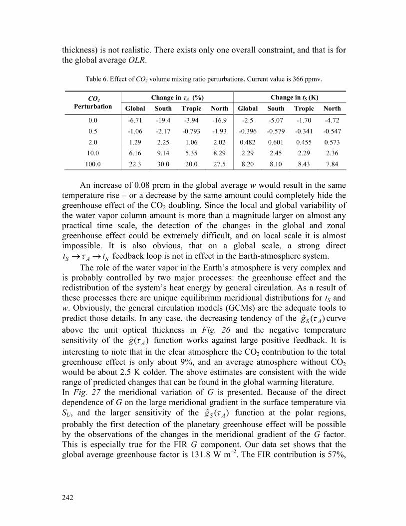
242

thickness) is not realistic. There exists only one overall constraint, and that is for the global average OLR.

Table 6. Effect of CO2 volume mixing ratio perturbations. Current value is 366 ppmv.

Change in τA (%) Change in tS (K) CO2 Perturbation Global South Tropic North Global South Tropic North

0.0 -6.71 -19.4 -3.94 -16.9 -2.5 -5.07 -1.70 -4.72 0.5 -1.06 -2.17 -0.793 -1.93 -0.396 -0.579 -0.341 -0.547 2.0 1.29 2.25 1.06 2.02 0.482 0.601 0.455 0.573

10.0 6.16 9.14 5.35 8.29 2.29 2.45 2.29 2.36 100.0 22.3 30.0 20.0 27.5 8.20 8.10 8.43 7.84

An increase of 0.08 prcm in the global average w would result in the same

temperature rise – or a decrease by the same amount could completely hide the greenhouse effect of the CO2 doubling. Since the local and global variability of the water vapor column amount is more than a magnitude larger on almost any practical time scale, the detection of the changes in the global and zonal greenhouse effect could be extremely difficult, and on local scale it is almost impossible. It is also obvious, that on a global scale, a strong direct

S A St tτ→ → feedback loop is not in effect in the Earth-atmosphere system. The role of the water vapor in the Earth’s atmosphere is very complex and

is probably controlled by two major processes: the greenhouse effect and the redistribution of the system’s heat energy by general circulation. As a result of these processes there are unique equilibrium meridional distributions for tS and w. Obviously, the general circulation models (GCMs) are the adequate tools to predict those details. In any case, the decreasing tendency of the ˆ ( )S Ag τ curve above the unit optical thickness in Fig. 26 and the negative temperature sensitivity of the ˆ ( )Ag τ function works against large positive feedback. It is interesting to note that in the clear atmosphere the CO2 contribution to the total greenhouse effect is only about 9%, and an average atmosphere without CO2 would be about 2.5 K colder. The above estimates are consistent with the wide range of predicted changes that can be found in the global warming literature. In Fig. 27 the meridional variation of G is presented. Because of the direct dependence of G on the large meridional gradient in the surface temperature via SU, and the larger sensitivity of the ˆ ( )S Ag τ function at the polar regions, probably the first detection of the planetary greenhouse effect will be possible by the observations of the changes in the meridional gradient of the G factor. This is especially true for the FIR G component. Our data set shows that the global average greenhouse factor is 131.8 W m–2. The FIR contribution is 57%,

243

and the shares of the MIR and WIN spectral ranges are 24% and 19%, respectively.

Fig. 27. Latitudinal dependence of the total and spectral greenhouse factors.

In Fig. 28 the meridional distribution of the total and spectral GN and the ˆ ( )Ag τ functions are plotted. The spectral GN curves show the relative

contributions to GN from the FIR, MIR, and WIN regions. According to this figure, the total GN is decreasing poleward from about 38% at the equatorial regions to about 15–20% at high latitudes. This behavior is obvious since decreasing water vapor content will increase the atmospheric infrared transparency almost everywhere in the longwave spectrum. The remarkably good agreement between the theoretically predicted greenhouse function and the simulated total normalized greenhouse factors further emphasize our earlier result, i.e., for zonal and global means the radiative equilibrium condition approximately holds.

While the total GN decreases poleward by about fifty percent, the far infrared contribution will increase from about 55% (of the total GN) at the equatorial regions to 70% at +/–80° latitudes. This increase, and the decrease of the MIR and WIN components, are due to the shift of the peak of the blackbody function toward the far infrared with decreasing temperature.

The WIN GN must also be affected by the ozone absorption, and theoretically, it should reflect the global average meridional distribution of the total ozone amount and the effective height of the ozone layer. Unfortunately, our data set does not contain sufficient information to explore these details.

244

Fig. 28. Latitudinal distributions of the total and spectral normalized greenhouse factors. The full circles are computed by Eq. 8.

4.3 Inverse terrestrial flux transmittance The inverse terrestrial flux transmittance as another greenhouse parameter was introduced by Stephens and Greenwald (1991). Based on the functional relationship between IT and GN , this parameter does not contain any more information about the greenhouse effect than GN and can not be related to the graybody atmospheric optical thickness in a simple way either. Theoretically IT has a nonlinear relationship with the atmospheric graybody optical thickness:

1 1ˆ( )2

AA

T AeI fτττ −−+ +′′ = = . (10)

In Fig. 29 the total IT as the function of w is plotted with dots. According to

Stephens and Greenwald (1991), the inverse terrestrial flux transmittance (IT) may be related to the terrestrial graybody optical thickness of the atmosphere, and consequently, it is directly related to the atmospheric water vapor content. In Stephens et al. (1993) a linear relationship in the form of TI a c w′ = + ∗ was also assumed, where a and c are regression constants. Based on satellite observations of OLR, w, and sea surface temperature, Stephens obtained the global annual mean distribution of TI and computed the regression coefficients a and c for the year of 1989. His results are also displayed in Fig. 29 as open circles.

245

Fig. 29. Dependence of inverse terrestrial flux transmittance on water vapor column amount.

The thin solid line in the plot, which is representing the total simulated IT,

was obtained by a linear fit using the points falling within the 1.0–5.0 prcm range. Regarding all the assumptions we made, and the accuracy of the satellite derived quantities in Stephens et al. (1993), this agreement is excellent, and at least in the 1–5 prcm range of w, the linear parameterization of the global greenhouse effect by the TI ′ quantity looks adequate. However, the simple two-parameter characterization of the planetary greenhouse effect by TI ′ for the full range of variability of w is not sufficient. Note, that Stephens curve fails to converge properly to 1.0 at low optical thickness, which is expected by the theoretical value TI ′′ . This tendency is reproduced pretty well by the simulated values.

4.4 Greenhouse temperature changes The clear indication of the presence of the planetary greenhouse effect is the fact, that the global average surface temperature is much higher than the effective planetary temperature which is computed from the global average OLR. As we have shown in the introduction, using the ERBE data one may easily estimate the effective planetary temperature.

The temperature difference, using an estimated 288 K global average surface temperature will result in an all-sky planetary greenhouse effect of 35 K. This corresponds to a global average g factor of 0.4 .

246

Fig. 30. Dependence of greenhouse temperature rise on water vapor column amount.

In our data set tE equals to 257.7 K, and tG equals to 285.3 K. The tem-

perature difference – we may call it clear-sky greenhouse temperature rise – is 27.91G G Edt t t= − = K, which is consistent with the theoretically predicted

value: 0.25ˆ[ /(1 ) / ] 27.5G Edt OLR g tσ= − − = K, and g is obtained from Eq. (8). The dependence of the local Gdt – computed as the difference of the local surface temperatures and effective temperatures – on the water vapor column amount is given in Fig. 30.

There are several possibilities to partition the Gdt function into the FIR, MIR, and WIN spectral regions. Here the Gdt components are weighted values with the corresponding spectral components of AA. The Gdt dependence on w is non-linear, and at higher w, Gdt exhibits some saturation tendency, obviously related to the thermodynamic control of the column water amount. The greenhouse effect can be parameterized with sufficient accuracy via w, tS, and O3. If one insists on using simple formulas, Eq. (22) in Table 4 reproduces the total greenhouse temperature rise with a correlation coefficient of 0.913. In this case the dependence on tS and O3 was ignored. The temperature differences computed from the downward and upward atmospheric emittances would produce practically the same results, therefore, we did not plot it in this figure.

The latitudinal variation of Gdt is presented in Fig. 31. The markers are the three degree zonal averages of the total Gdt . The major contributions to Gdt come from the FIR and WIN components, and the relatively sharp peak at the tropical area is caused by the WIN component. The much smaller latitudinal

247

changes in the FIR and MIR components could be related to the same compensation mechanism affecting the FIR and MIR OLRs.

There are further possibilities to express the magnitude of the greenhouse effect for example, via the total absorbed flux density of the atmosphere,

A U T UA S S S A= − = , or the downward atmospheric emittance ED, see Fig. 20. In Fig. 32, we plot the quantity of ˆA S Adt t t= − , as the function of w. Here ˆAt may be called as the clear-sky brightness temperature, computed from the total absorbed flux density using the Stefan-Boltzmann law. This figure expresses the fact that with increasing w the surface is getting closer to the radiative equilibrium with the atmosphere. All over the range of w the FIR spectral range is the major contributor to the total dtA.

Just like in the case of the dtG, these curves are also showing some tendency for saturation at larger w. This tendency, as we mentioned already, is related to the direct thermodynamic control of the water vapor column amount. In Fig. 32 the tS(dtA) function is also plotted with a thin line. The extrapolation of this curve toward the dtA = 0 line (dashed part of the curve) will point to the critical values of tS and w, where the radiative cooling of the surface stops. Based on our data set, these values are 303.8 K and 7.38 prcm, respectively. According to the minimum value of dtA – which is 3.77 K, and marked with a short horizontal line – such situation in the Earth’s atmosphere is not likely to happen. Before reaching the above limits, the more efficient thermodynamic and transport processes will take over the re-distribution of the local surface heat energy and the water vapor amount.

Fig. 31. Latitudinal variation of the greenhouse temperature rise, dtG.

248

Fig. 32. Dependence of greenhouse temperature change, dtA, on water vapor column amount and surface temperature.

None of the above discussed greenhouse parameters are better than the

other. Which one to use largely depends on the available data and the nature of the radiative transfer problem at hand. It must be clear, that the greenhouse effect is a large scale phenomenon which requires the existence of the radiative equilibrium as a constraint, both for the temperature profile and the OLR. Eqs. (1)–(10) are only valid under the radiative equilibrium condition. Our results show that for global and zonal averages this condition approximately holds. The chances are very little to randomly select an individual vertical air column with its temperature profile in IR radiative equilibrium and measure the greenhouse effect.

Unfortunately, within the frame of this paper we could not go into the full mathematical details of the solution of the Schwazschild-Milne equations and the mathematical proofs of the new equations.

5. Conclusions

Besides the number of interesting details, the most significant result of this research was to establish a qualitative picture of the clear-sky spectral radiative properties of the Earth-atmosphere system in the three most important spectral regions. Several simple and accurate formulas of different physical quantities have been developed for direct use in practical applications. The basic tendency of the meridional variations of the FIR, MIR, and WIN spectral components

249

were derived. We derived fundamental theoretical relationships that strongly supported the simulation results on the H2O and CO2 greenhouse effects. These results could be valuable contributions to the general global picture given by Hansen (1998), Paltridge and Platt (1976), or Peixoto and Oort (1992), or by several others who were not mentioned here. The application of our transfer and greenhouse functions in GCM climate simulations may also improve our understanding of the greenhouse effect in the Earth’s atmosphere.

Equations related to the semi-infinite atmospheric model were replaced with new relationships valid for the semi-transparent atmosphere. With the help of the newly introduced transfer and greenhouse functions we established the connection between the theoretical and empirical greenhouse parameters. Probably the most important consequence of the semi-transparent atmospheric model is the significant reduction in the expected response in the surface upward flux to greenhouse gas perturbations.

Obviously, the presented results have their limitations. The most significant one is related to the temperature profile data base. In some latitudinal belts we had rather few soundings, therefore, it is difficult to set up selection procedures to obtain statistically consistent data sets for each latitudinal belts. There are virtually unlimited possibilities in increasing the complexity of such simulations by involving more atmospheric and surface parameters. The scientific community dealing with the present and future of the greenhouse effect of the Earth’s atmosphere would certainly welcome such extensions of this kind of research. A similar study which deals with the cloud effect is also desirable.

Using an LBL code for the radiative transfer computations was also crucial. The fine details of the transitions of the flux transmittances from the opaque to the transparent spectral regions, especially at higher altitudes, can only be traced with correct mathematical representation of the infrared radiative transfer. Although the speed of computers are improving, the computational burden of doing such simulations on much larger data sets could be a concern.

The presented results in the FIR spectral range are awaiting the confirmation by direct observations. Apparently in the FIR region there is a kind of spectral compensation in effect which prevents the FIR OLR to dramatically respond to the poleward temperature decrease. However, statements on the variability of the FIR OLR must be supported by a solid FIR climatology, which is based on direct observations. The predicted meridional variation in the total and spectral transmitted flux densities should also be supported by observations. The role of the FIR and WIN spectral regions in forming the greenhouse temperature rise is obvious. One should not forget that the boundaries of the spectral ranges are unique, and changing these boundaries will alter the contributions of the different spectral components. The most critical wave number is the one which separates FIR and WIN regions.

250

In general, the qualitative picture given above must be validated against direct satellite measurements especially in the FIR spectral range. The first opportunity to gather satellite measured fluxes in the FIR spectral range has just arrived. The utilization of the differences of the coincidental flux measurements from the Terra and Aqua satellites will give us the first measured global radiative fluxes in this important spectral region.

Acknowledgements—This research was supported by the NASA Science Mission Directorate through the EOS project, (contract No. NAS1-02058). Support was also received from M. Kurylo, D. Anderson, and H. Maring at NASA HQ. We are very grateful to S. Gupta at AS&M for his helpful discussions regarding the scientific and technical details of the manuscript.

References Brindley, H.E. and Harries, J.E., 1997: The impact of far infra-red absorption on greenhouse forcing:

sensitivity studies at high spectral resolution. In IRS'96 Current Problems in Atmospheric Radiative Transfer. Deepak pub., 981-984.

Brutsaert, W., 1975: On a derivable formula for longwave radiation from clear skies. Water Resources Research 11, 742-744.

Chedin, A. and Scott, N. A., 1983: The Improved Initialization Inversion Procedure. Laboratoire de meteorologie dynamique. Centre National de la Recherche Scientifique, No. 117.

Collins, II, G.W., 2003: The fundamentals of Stellar Astrophysics. Part II. Stellar Atmospheres. WEB edition.

COVE, 2003: COVE Time Synchronized Monthly Archive Files, http://www-svg.larc.nasa.gov. ERBE, 2004: ERBE Monthly Scanner Data Product. NASA Langley Research Center, Langley DAAC

User and Data Services, userserv@eosdis.larc.nasa.gov. Goody, R.M. and Yung, Y.L., 1989: Atmospheric Radiation. Theoretical Basis. Oxford University

Press, Inc. Gupta, S.K., 1989: A parameterization for longwave surface radiation from Sun-synchronous satellite

data. J. Climate 2, 305-319. Gupta, S.K., Darnell, W.L., and Wilber, A.C., 1992: A parameterization for longwave surface radiation

from satellite data: recent improvements. JAM, Vol. 31, No. 12, 1361-1367. Hansen, J.E., Sato, M., Lacis, A., Ruedy, R., Tegen, I., and Matthews, E., 1998: Climate forcings in the

industrial era. Proc. Natl. Acad. Sci. USA, Vol. 95, 12753-12758. HITRAN2K, 2002; http://cfa-www.Harvard.edu/HITRAN/hitrandata. Husson, N., Bonnet, B., Chedin, A., Scott, N., Chursin, A.A., Golovko, V.F., and Tyuterev, V.G., 1994:

The GEISA databank in 1993: a PC/AT compatible computers’ new version. J. Quant. Spectrosc. Ra. 52, 425-438.

Idso, S.B., 1981: A set of equations for full spectrum and 8-14 µ and 10.5-12.5 µ thermal radiation from cloudless skies. Water Resour. Res. 17, 295-304.

Kiehl, J.T. and Trenberth, K.E., 1997: Earth’s annual global mean energy budget. B. Am. Meteorol. Soc. 78, No. 2, February.

Kratz, D.P., Mlynczak, M.G., Mertens, C.J., Brindley, H., Gordley, L.L., Martin-Torres, J., Miskolczi, F.M., Turner, D.D., 2005: An inter-comparison of far-infrared line-by-line radiative transfer models. J.Q.S.R.T., 90 (2005) 323-341

Miskolczi, F., Bonzagni, M., and Guzzi, R., 1990: High-resolution atmospheric radiance-transmittance code (HARTCODE). In Meteorology and Evironmental Sciences: Proc. of the Course on Physical Climatology and Meteorology for Environmental Application. World Scientific Publ. Co. Inc., Singapore, 743-790.

251

Miskolczi, F. and Rizzi, R., 1998: High accuracy skin temperature retrieval using spectral measurements of multi-channel imagers. International Radiation Symposium 1998, Madison, Wisconsin, USA.

Paltridge, G.W. and Platt, C.M., 1976: Radiative Processes in Meteorology and Climatology. Elsevier Scientific Publishing Company.

Peixoto, J.P. and Oort, A.H., 1992: Physics of Climate. American Institute of Physics, NewYork. Raval, A. and Ramanathan, V., 1989: Observational determination of the greenhouse effect. Nature

342. Rizzi, R., Matricardi, M., and Miskolczi, F., 2002: On the simulation of up-looking and down-looking

high-resolution radiance spectra using two different radiative transfer models. Appl. Optics 41, 940-956.

Rodriguez, R., Jucks, K.W., Lacome, N., Blanquest, G., Valrand, J., Traub, W.A., Khalil, B., LeDoucent, R., Valentin, A., Camy-Peyret, C., Bonamy, L., and Hartmann J.M., 1999: Model, software, and data-base for computation of line-mixing effects in infrared Q branches of atmospheric CO2. I. Symmetric isotopomers. J. Quant. Spectrosc. Ra. 61, 153-184.

Rothman L.S., Rinsland, C.P., Goldman, A., Massie, T., Edwards, D.P., Flaud, J-M., Perrin, A., Camy-Peyret, C., Dana, V., Mandin, J-Y., Schroeder, J., Cann, A., Gamache, R.R., Wattson, R.B., Yoshio, K., Chance, K.V., Jucks, K.W., Brown, L.R., Nemtchinov, V., and Varansi, P., 1998: The HITRAN molecular spectroscopic database and HAWKS (HITRAN atmospheric workstation): 1996 edition. J. Quant. Spectrosc. Ra. 60, 665-710.

Rozanov, A., 2001: Modeling of Radiative Transfer through a Spherical Planetary Atmosphere: Application to Atmospheric Trace Gases Retrieval from Occultation- and Limb-measurements in UV-Vis-NIR. Dissertation, Institut fur Umweltphysik, Universitat Bremen.

Rutten, R.J., 2000: Radiative Transfer in Stellar Atmospheres. Lecture notes, Utrecht University. 7th edition.

Schneider, E.K., Kirtman, B.P., and Lindzen, R.S., 1999: Tropospheric water vapor and climate sensitivity. J. Atmos. Sci. 56, 1650.

Stephens, G.L. and Greenwald, T.J., 1991: The Earth's radiation budget and its relation to atmospheric hydrology. 1. Observations of the clear-sky greenhouse effect. JGR Vol. 96 No. D8.

Stephens, G.L., Slingo, A., and Webb, M., 1993: On measuring the greenhouse effect of Earth. NATO ASI Series, Vol. 19.

Tobin, D.C., Best, F.A., Brown, P.D., Dedecker, R.G., Ellingson, R.G., Garcia, R.K., Howell, H.B., Knuteson, R.O., Mlawer, E.J., Revercomb, H.E., Short, J.F., Van Delst, P.F.W., and Walden, V.P., 1999: Down-welling spectral radiance observations at the SHEBA ice station: Water vapor continuum measurements from 17 to 26 µm. J. Geophys. Res. 104, No. D2, 2081-2092.

Tuzet, A., 1990: A simple method for estimating downward longwave radiation from surface and satellite data by clear skies. Int. J. Remote Sens. 11, 125-131.

Vonder Haar, T., 1986: WCP 115, WMO ITD, No. 109, pp. 144.