THE GRAND UNIFIED THEORY - brilliantlightpower.com · 12/10/2018 · iii 35.17 Analytical...
358
Transcript of THE GRAND UNIFIED THEORY - brilliantlightpower.com · 12/10/2018 · iii 35.17 Analytical...

THE GRAND UNIFIED THEORY
OF CLASSICAL PHYSICS
Volume 3 of 3


THE GRAND UNIFIED THEORY OF CLASSICAL PHYSICS
BY
Dr. Randell L. Mills
December 10, 2018 Edition
Volume 3 of 3
Copyright © 2018 by Dr. Randell L. Mills
All rights reserved. No part of this work covered by copyright hereon may be reproduced or used in any form, or by any means-graphic, electronic, or mechanical, including photocopying, recording, taping, or information storage and retrieval systems-without written permission of Dr. Randell L. Mills. Manufactured in the United States of America.
ISBN 978-0-9635171-5-9 Library of Congress Control Number 2015915593


i
TABLE OF CONTENTS
VOLUME 3 COLLECTIVE PHENOMENA, HIGH-ENERGY PHYSICS, & COSMOLOGY 24. Statistical Mechanics .................................................................................................................................................. 1409 24.1 Three Different Kinds of Atomic-Scale Statistical Distributions ................................................................... 1409 24.1.1 Maxwell-Boltzmann ..................................................................................................................... 1410 24.1.2 Bose-Einstein ................................................................................................................................ 1411 24.1.3 Fermi-Dirac ................................................................................................................................... 1411
24.2 Application of Maxwell-Boltzmann Statistics to Model Molecular Energies in an Ideal Gas ....................... 1414 24.3 Application of Bose-Einstein Statistics to Model Blackbody Radiation ........................................................ 1417 24.3.1 Planck Radiation Law ................................................................................................................... 1418 24.4 Application of Bose-Einstein Statistics to Model Specific Heats of Solids ................................................... 1421 24.5 Application of Fermi-Dirac Statistics to Model Free Electrons in a Metal .................................................... 1422 24.5.1 Electron-Energy Distribution ........................................................................................................ 1423 References ................................................................................................................................................................... 1424 25. Superconductivity ....................................................................................................................................................... 1425 Box 25.1 Fourier Transform of the System Function ............................................................................................... 1425 References ................................................................................................................................................................... 1428 25.1 Band-Pass Filter .............................................................................................................................................. 1428 25.2 Critical Temperature, Tc ................................................................................................................................. 1432
25.2.1 Tc for Conventional Three Dimensional Metallic Superconductors ............................................ 1432 25.2.2 Tc for One, Two, or Three Dimensional Ceramic Oxide Superconductors ................................ 1432 25.3 Josephson Junction, Weak Link ...................................................................................................................... 1432 References ................................................................................................................................................................... 1433 26. Quantum Hall Effect ................................................................................................................................................... 1435 26.1 General Considerations ................................................................................................................................... 1435 26.2 Integral Quantum Hall Effect .......................................................................................................................... 1436 26.3 Fractional Quantum Hall Effect ...................................................................................................................... 1439 References ................................................................................................................................................................... 1440 27. Aharonov-Bohm Effect ............................................................................................................................................... 1441 References ................................................................................................................................................................... 1443 28. Creation of Matter from Energy ................................................................................................................................. 1445 29. Pair Production............................................................................................................................................................ 1449 References ................................................................................................................................................................... 1452 30. Positronium ................................................................................................................................................................. 1453 30.1 Excited State Energies .................................................................................................................................... 1454 30.2 Hyperfine Structure ......................................................................................................................................... 1455 References ................................................................................................................................................................... 1457 31. Relativity ..................................................................................................................................................................... 1459 31.1 Basis of a Theory of Relativity ............................................................................................................................. 1459 31.2 Lorentz Transformations ................................................................................................................................. 1462 31.3 Time Dilation .................................................................................................................................................. 1462 31.3.1 The Relativity of Time .................................................................................................................. 1462 31.4 The Relativity Principle and the Covariance of Equations in Galilean or Euclidean Spacetime and Riemann Spacetime .................................................................................................................................. 1464 References ................................................................................................................................................................... 1468 32. Gravity ........................................................................................................................................................................ 1469 32.1 Quantum Gravity of Fundamental Particles ................................................................................................... 1469 32.2 Particle Production .......................................................................................................................................... 1477 Box 32.1 Definition of Time Unit Sec, and Calculation and Measurement of Observables Over All Scales Thereupon ...................................................................................................................................... 1479 Box 32.2 Relationships Between the Earth Mean Solar Day Definition of the Second, the Definition of Sec Based on Pair Production and its Effect on Spacetime, and the Definition of Sec and the Fundamental Constants ....................................................................................................................... 1480 32.3 Orbital Mechanics ........................................................................................................................................... 1482 32.4 Relativistic Corrections of Newtonian Mechanics and Newtonian Gravity ................................................... 1483 32.5 Precession of the Perihelion ............................................................................................................................ 1484

ii
32.6 Deflection of Light .......................................................................................................................................... 1486 32.7 Cosmology ...................................................................................................................................................... 1488
32.8 Failed Cosmological Predictions Reveal Einstein’s Incorrect Physical Basis of General Relativity ............. 1490 32.9 Cosmology Based on the Relativistic Effects of Matter/Energy Conversion on Spacetime .......................... 1494 32.9.1 The Arrow of Time and Entropy .................................................................................................. 1494 32.9.2 The Arrow of Time ....................................................................................................................... 1494 32.9.3 The Expanding Universe and the Microwave Background .......................................................... 1495 32.9.4 The Period of Oscillation Based on Closed Propagation of Light ................................................ 1498 32.9.5 Equations of the Evolution of the Universe .................................................................................. 1498 Box 32.3 Simplified Set of Cosmological Equations ............................................................................................... 1505 32.10 Composition of the Universe .......................................................................................................................... 1508 32.11 Power Spectrum of the Cosmos ...................................................................................................................... 1514 32.12 The Differential Equation of the Radius of the Universe ............................................................................... 1515 32.13 Power Spectrum of the Cosmic Microwave Background ............................................................................... 1518 References ................................................................................................................................................................... 1525 33. Unification of Spacetime, the Forces, Matter, and Energy ......................................................................................... 1531 33.1 Relationship of Spacetime and the Forces ...................................................................................................... 1531 33.2 Relationship of Spacetime, Matter, and Charge ............................................................................................. 1533 33.3 Period Equivalence ......................................................................................................................................... 1535 33.4 Wave Equation ................................................................................................................................................ 1537 References ................................................................................................................................................................... 1537 34. Equivalence of Inertial and Gravitational Masses Due to Absolute Space and Absolute Light Velocity .................. 1539 34.1 Newton’s Absolute Space Was Abandoned by Special Relativity Because Its Nature Was Unknown ......... 1539 34.2 Relationship of the Properties of Spacetime and the Photon to the Inertial and Gravitational Masses .......... 1542 34.2.1 Lorentz Transforms Based on Constant Relative Velocity ........................................................... 1542 34.2.2 Minkowski Space .......................................................................................................................... 1543 34.2.3 Origin of Gravity with Particle Production ................................................................................... 1544 34.2.4 Schwarzschild Space and Lorentz-type Transforms Based on the Gravitational Velocity at Particle Production .................................................................................................................... 1544 34.2.5 Particle Production Continuity Conditions from Maxwell’s Equations, and the Schwarzschild Metric Give Rise to Charge, Momentum and Mass ............................................. 1547 34.2.6 Relationship of Matter to Energy and Spacetime Expansion ....................................................... 1549 34.2.7 Cosmological Consequences ........................................................................................................ 1549 34.2.8 The Period of Oscillation of the Universe Based on Closed Propagation of Light ...................... 1549 34.2.9 The Differential Equation of the Radius of the Universe ............................................................. 1550 34.2.10 The Periods of Spacetime Expansion/Contraction And Particle Decay/Production for the Universe Are Equal ........................................................................................................... 1550 34.3 Equivalence of the Gravitational and Inertial Masses .................................................................................... 1551 34.4 Newton’s Second Law .................................................................................................................................... 1553 34.5 Return to the Twin Paradox ............................................................................................................................ 1554 34.6 Absolute Space Confirmed Experimentally .................................................................................................... 1555 References ................................................................................................................................................................... 1555 35. The Fifth Force ........................................................................................................................................................... 1557 35.1 General Considerations ................................................................................................................................... 1557 35.2 Positive, Zero, and Negative Gravitational Mass ........................................................................................... 1561 35.3 Determination of the Properties of Electrons, Those of Constant Negative Curvature, and Those of Pseudeoelectrons ............................................................................................................................................. 1564 35.4 Nature of Photonic Super Bound Hydrogen States and the Corresponding Continuum Extreme
Ultraviolet (EUV) Transition Emission and Super Fast Atomic Hydrogen ................................................... 1565 35.5 Nature of Photon-Bound Autonomous Electron States .................................................................................. 1567 35.6 Pseudoelectrons............................................................................................................................................... 1568 35.7 Fourier Transform of the Pseudoelectron Current Density ............................................................................. 1570 35.8 Force Balance and Electrical Energies of Pseudoelectron States ................................................................... 1571 35.9 Tri-Hydrogen Cation Relativistic Electron Collision Pseudoelectron Mechanism ........................................ 1577 References ................................................................................................................................................................... 1583 36. Leptons ........................................................................................................................................................................ 1585 36.1 The Electron-Antielectron Lepton Pair ........................................................................................................... 1586 36.2 The Muon-Antimuon Lepton Pair .................................................................................................................. 1587 36.3 The Tau-Antitau Lepton Pair .......................................................................................................................... 1587 36.4 Relations Between the Leptons ....................................................................................................................... 1588 36.5 X17 Particle .................................................................................................................................................... 1589

iii
References ................................................................................................................................................................... 1590 37. Proton and Neutron ..................................................................................................................................................... 1591 37.1 Quark and Gluon Functions ............................................................................................................................ 1592 37.1.1 The Proton ..................................................................................................................................... 1593 37.1.2 The Neutron .................................................................................................................................. 1595 37.2 Magnetic Moments ......................................................................................................................................... 1596 37.2.1 Proton Magnetic Moment ............................................................................................................. 1596 37.2.2 Neutron Magnetic Moment ........................................................................................................... 1597 37.3 Neutron and Proton Production ...................................................................................................................... 1598 37.4 Intermediate Vector and Higgs Bosons .......................................................................................................... 1600 References ................................................................................................................................................................... 1601 38. Quarks ......................................................................................................................................................................... 1603 38.1 Down-Down-Up Neutron (ddu) ...................................................................................................................... 1604 38.2 Strange-Strange-Charm Neutron (ssc) ............................................................................................................ 1604 38.3 Bottom-Bottom-Top Neutron (bbt)................................................................................................................. 1605 38.4 Relations Between Members of the Neutron Family and the Leptons ........................................................... 1606 References ................................................................................................................................................................... 1607 39. Nuclear Forces and Radioactivity ............................................................................................................................... 1609 39.1 The Weak Nuclear Force: Beta Decay of the Neutron ................................................................................... 1609 39.1.1 Beta Decay Energy ....................................................................................................................... 1609 39.1.2 Neutrinos ....................................................................................................................................... 1610 39.2 The Strong Nuclear Force ............................................................................................................................... 1617 39.2.1 The Deuterium Nucleus ............................................................................................................... 1617 39.3 Nuclear and X-ray Multipole Radiation ......................................................................................................... 1618 39.4 K-Capture ........................................................................................................................................................ 1620 39.5 Alpha Decay .................................................................................................................................................... 1621 39.5.1 Electron Transmission and Reflection at a Potential Energy Step ............................................... 1621 39.5.2 Transmission (Tunneling) Out of a Nucleus—Alpha Decay ........................................................ 1623 References ................................................................................................................................................................... 1625 RETROSPECT 40. Retrospect: The Schrödinger Wave function in Violation of Maxwell’s Equations ................................................. 1627 References ................................................................................................................................................................... 1628 41. Retrospect: Classical Electron Radius ....................................................................................................................... 1629 References ................................................................................................................................................................... 1630 42. Retrospect: Wave-Particle Duality ............................................................................................................................ 1631 42.1 The Wave-Particle Duality is Not Due to the Uncertainty Principle ............................................................ 1634 42.2 Inconsistencies of Quantum Mechanics.......................................................................................................... 1638 42.3 The Aspect Experiment—No Spooky Actions at a Distance ......................................................................... 1640 42.3.1 Aspect Experimental Results Are Predicted Classically .............................................................. 1643
42.3.2 Aspect Experimental Results Are Not Predicted by Quantum Mechanics ................................... 1645 42.4 Bell’s Theorem Test of Local Hidden Variable Theories (LHVT) and Quantum Mechanics ....................... 1646 42.5 Wheeler: Back to Reality Not Back to the Future .......................................................................................... 1648 42.5 Schrödinger “Black” Cats ............................................................................................................................... 1651 42.5.1 Experimental Approach ............................................................................................................... 1652 42.5.2 State Preparation and Detection ................................................................................................... 1654 42.6 Schrödinger Fat Cats—Another Flawed Interpretation .................................................................................. 1660 42.6.1 Superconducting Quantum Interference Device (SQUID) ........................................................... 1661 42.6.2 Experimental Approach ................................................................................................................ 1662 42.6.3 Data ............................................................................................................................................... 1663 42.6.4 Quantum Interpretation ................................................................................................................. 1664 42.6.5 Classical Interpretation ................................................................................................................. 1664 42.7 Classical All the Way Up ................................................................................................................................ 1667 42.8 Free Electrons in Superfluid Helium are Real in the Absence of Measurement Requiring a Connection of Ψ(x) to Physical Reality .............................................................................................................................. 1669 42.8.1 Stability of Fractional-Principal-Quantum States of Free Electrons in Liquid Helium ................ 1671 42.8.2 Ion Mobility Results in Superfluid Helium Match Predictions .................................................... 1672 42.9 One Dimension Gravity Well—Another Flawed Interpretation ..................................................................... 1679 42.10 Physics is Not Different on the Atomic Scale ................................................................................................ 1681 References ................................................................................................................................................................... 1682

iv
APPENDICES Appendix I: Nonradiation Condition ............................................................................................................................ 1685 Ap. I.1 Derivation of the Condition of Nonradiation ................................................................................ 1685 Ap. I.2 Spacetime Fourier Transform of the Electron Function ............................................................... 1685 Ap. I.3 Nonradiation Based on the Electromagnetic Fields and the Poynting Power Vector ................................................................................................................ 1689 References ................................................................................................................................................. 1695 Appendix II: Stability and Absence of Self Interaction and Self Energy ....................................................................... 1697 Ap. II.1 Stability ................................................................................................................................... 1697 Ap. II.2 Self Interaction ........................................................................................................................ 1698 Ap. II.2.1 Gauss’ Law in Two Dimensions Equates a Discontinuous Field Due to a Discontinuous Charge Layer Source ............................................................ 1699 Ap. II.2.2 Self Force Due to a Layer of Charge with Nonzero Thickness ...................... 1700 Ap. II.2.3 Conditions for the Absence or Presence of a Self Force Using Coulomb’s Law ............................................................................................... 1702 Ap. II.3 Self Energy.............................................................................................................................. 1705 References ................................................................................................................................................. 1706 Appendix III: Muon g Factor ........................................................................................................................................... 1709 Ap. III.1 Experimental Determination of the Proper .......................................................................... 1714 References ................................................................................................................................................. 1714 Appendix IV: Analytical Equations to Generate the Free Electron Current-Vector Field and the Angular-Momentum-Density Function 0
0 ( , )Y ..................................................................................... 1715
Ap. IV.1 Rotation of a Great Circle in the xy-Plane about the ,0 ,x y zi i i -Axis by 2 ...................... 1715
Ap. IV.1.1 Conical Surfaces Formed by Variation of ................................................. 1717
Ap. IV.2 Rotation of a Great Circle in the xy-Plane about the ,0 , x y zi i i -Axis by 2 .................... 1717
Ap. IV.2.1 Conical Surfaces Formed by Variation of ................................................. 1719
Ap. IV.3 The Momentum-Density Function 00 ,Y .......................................................................... 1719
Ap. IV.3.1 Matrices to Visualize the Momentum-Density of 00 ,Y
for the Combined Precession Motion of the Free Electron
About the ,0 ,x y zi i i -Axis and z-Axis .......................................................... 1720
Ap. IV.3.2 Convolution Generation of 00 ,Y .............................................................. 1721
Ap. IV.3.3 Matrices to Visualize the Momentum-Density of 00 ,Y
for the Combined Precession Motion of the Free Electron About the ,0 , x y zi i i -Axis and z-Axis ........................................................ 1723
Ap. IV.3.4 Azimuthal Uniformity Proof of 00 ,Y ....................................................... 1725
Ap. IV.3.5 Spin Flip Transitions ....................................................................................... 1726 References ................................................................................................................................................. 1727 Appendix V: Analytical-Equation Derivation of the Photon Electric and Magnetic Fields .......................................... 1729 Ap. V.1 Analytical Equations to Generate the Right-Handed Circularly-Polarized Photon Electric and Magnetic Vector Field by the Rotation of the Great-Circle Basis Elements
about the , ,0x y zi i i -Axis by 2
............................................................................................ 1729
Ap. V.2 Analytical Equations to Generate the Left-Handed Circularly-Polarized Photon Electric and Magnetic Vector Field by the Rotation of the Great-Circle Basis Elements
about the , ,0x y zi i i -Axis by 2
......................................................................................... 1731
Ap. V.3 Generation of the Linearly-Polarized Photon Electric and Magnetic Vector Field ............... 1734 Ap. V.4 Photon Fields in the Laboratory Frame .................................................................................. 1734 References ................................................................................................................................................. 1737 Appendix VI: The Relative Angular Momentum Components of Electron 1 and Electron 2 of Helium to Determine the Magnetic Interactions and the Central Magnetic Force .................................................... 1739
Ap. VI.1 Singlet Excited States with = 0 ( 12 11 1s s ns ) ............................................................... 1739

v
Ap. VI.2 Triplet Excited States with = 0 ( 12 11 1s s ns ) ................................................................ 1743
Ap. VI.3 Singlet Excited States with ≠ 0 ........................................................................................... 1747 Ap. VI.4 Triplet Excited States with ≠ 0 ............................................................................................ 1750 References ................................................................................................................................................. 1754

vi

1409
Chapter 24 STATISTICAL MECHANICS Large systems of particles are ubiquitous in nature. The physics of each particle of a large system is determined by physical laws given its initial conditions and history. However, the amount of information to follow even 2 grams of hydrogen gas having Avogadro’s number of molecules ( 23 16.022045 10 AN X mol ) is overwhelming. Statistical models typically deal with
insufficient information for an underlying deterministic macrosystem such as the determination of an average property of a population with the accuracy only limited by the number of independent samples1. Fortunately for the cases of atomic systems, it is also possible to determine the bulk properties of many systems using statistical models. The modeling of aggregate behavior of a large ensemble of atoms, electrons, or photons obeying classical physics such as molecules in a gas, photons in a cavity, and free electrons in a metal is the branch of physics called statistical mechanics. Statistical mechanics gives state properties of a system of many particles that are a manifestation of the properties of the particles themselves. The necessity to be concerned with the actual motions and interactions of individual particles is avoided. Instead, such models give predictions for the probability that the particle has a certain amount of energy at a certain moment. It gives statistical distributions for all of the particles rather than the exact value for a specific particle. THREE DIFFERENT KINDS OF ATOMIC-SCALE STATISTICAL DISTRIBUTIONS [5] It was shown in the State Lifetimes and Line Intensities section, that a mean lifetime arises due to the superposition of transitions over an ensemble of individual atoms. Each atom has an exact lifetime due to an exact transition involving specific initial, final, and any intermediate , m states and the corresponding exact photon in space relative to the states. The mean lifetime arises from the mean current given by Eq. (2.87) and the spherical radiation field due to the superposition of emitted photons. Similarly, Maxwell’s equations apply to macroscopic electromagnetic fields that are in actuality the superposition of quantized photons traveling at the speed of light. Furthermore, using Maxwell’s equations, the reduced speed of light in a transparent medium can be shown to be due to the radiation from many induced dipoles that produce a single wave propagating at the reduced speed [6]. Thus, deterministic physics arises as the aggregate behavior of entities that also in turn obey deterministic physics. The same principle applies in the case of statistical mechanical models.
In previous sections, the exact nature of individual particles (e.g. atoms, electrons, and photons) were solved. The interactions of two separate individual particles demonstrated three types of behavior that are correctly modeled by three types of corresponding statistical models. Each statistical model with a corresponding probability distribution function is based on the properties of the particle and their corresponding interactions. According to statistical thermodynamics [7], a macroscopic thermodynamic system is viewed as an assembly of myriad submicroscopic entities in ever changing quantum states. Consider the number of distinct ways that a set number of energy
1 Quantum theory is incompatible with probability theory since the latter is based on underlying unknown, but determined outcomes, and the former is not [1]. Wavefunction solutions of the Schrödinger equation are interpreted as probability-density functions. Quantum theory confuses the concepts of a wave and a probability-density function that are based on totally different mathematical and physical principles. The use of “probability” in this instance does not conform to the mathematical rules and principles of probability theory. Statistical theory is based on an existing deterministic reality with incomplete information; whereas, quantum measurement acts on a “probability-density function” to determine a reality that did not exist before the measurement. Additionally, it is nonsensical to treat a single particle such as an electron as if it was a population of electrons and to assign the single electron to a statistical distribution over many states. The electron has conjugate degrees of freedom such as position, momentum, and energy that obey conservation laws in an inverse-r Coulomb field. A single electron cannot have multiple positions and momenta or energies simultaneously. The decision to treat the electron as a point-particle-probability wave, a point with no volume with a vague probability wave requiring that the electron have an infinite number of positions and energies including negative and infinite energies simultaneously was a turning point in physics. The adoption of the probabilistic versus deterministic nature of atomic particles violates all physical laws including special relativity with violation of causality as pointed out by Einstein [2] and de Broglie [3]. Consequently, it was rejected even by Schrödinger [4]. Pure mathematics took the place of physics, but even so, the mathematics is not even consistent with probability theory.

Chapter 24
1410
quanta can be distributed between a set number of energy levels each called a microstate. The total number of microstates W associated with any configuration involving N distinguishable units is
!
! !a b
NW
(24.1)
where a represents the number of units assigned the same number of energy quanta (and, hence, occupying the same quantum
number), and b represents the number of units occupying some other quantum level. As the number of units increases, the total
number of microstates skyrockets to unimaginable magnitudes. Thus, one can calculate that an assembly of 1000 localized harmonic oscillators sharing 1000 energy quanta possesses more than 60010 different microstates. This explosive expansion of the total number of microstates with increasing N is a direct consequence of the mathematics of permutations, from which arises also a second consequence of no less importance. Statistical analysis shows that the emergence of a predominant configuration is characteristic of any assembly with a large number ( N ) of units. Of the immense total number of microstates that can be assumed by a large assembly, an overwhelming proportion arises from one comparatively, small set of configurations centered on, and only minutely different from, the predominant configuration—with which they share an empirically identical set of macroscopic properties.
The first step in the program of statistical mechanics is to find a general expression for W for the kind of particles being considered. Then W is maximized subject to the conditions that the system consists of a fixed number of N particles (except when they are photons or their acoustic equivalents called phonons where the total energy is conserved, but the number can change since the individual energies are given by Planck’s equation, E h ) and that the system contains a fixed amount of energy E that is conserved in populating the conserved number of states where applicable. The result in each case is an expression for n , the number of particles with the energy , that has the form:
n g f (24.2)
where g = number of states of energy
= statistical weight corresponding to energy f = distribution function
= average number of particles in each state of energy = probability of occupancy of each state of energy
When a continuous rather than a discrete distribution of energies is involved, g is replaced by g d , the number of states
energies between and d . Each of the three models is based upon the determination of the most probable way in which a certain total amount of
energy E is distributed among the N members of a system of particles in thermal equilibrium at the absolute temperature T . Then, it is possible to statistically predict aggregate properties such as the number of particles having an energy 1 , 2 , and so
on, based on the model. The particle interactions are assumed to be at thermal equilibrium between themselves and the walls of their container in the absence of strongly correlated motion. More than one particle state may have a certain energy . In the case of Maxwell-Boltzmann and Bose-Einstein statistics more than one particle may be in a certain state. In the case of Fermi-Dirac statistics each particle must be in different state since Fermi-Dirac statistics treats particles such as electrons that spin pair. A fundamental assumption of all statistical mechanical models that is supported by experimentation and consistent with physical laws, is that the greater the number W of different ways in which the particles can be arranged among the available states to yield a particular distribution of energies, the more probable the distribution. It is assumed that each state of a certain energy is equally likely to be occupied. The atomic scale distributions derived from deterministic, conditional probability theory [8] are: MAXWELL-BOLTZMANN—identical, discrete particles such as molecules are separated and act independently such that they possess a continuum of momenta with exchange by the predominant interaction of collisional scattering. Atoms and molecules have exact dimensions as shown in the and One-Electron Atom section, Two-Electron Atoms section, Three- Through Twenty-Electron Atoms section, Nature of the Chemical Bond of Hydrogen-Type Molecules and Molecular Ions section, Polyatomic Molecular Ions and Molecules section, and More Polyatomic Molecules and Hydrocarbons section. Neutral particles such as atoms and molecules undergo one-on-one collisional interactions, which are conservative; otherwise, there is no correlation between the separated particles. Maxwell-Boltzmann statistics is used to model the aggregate properties of a gas at a given temperature. The corresponding Maxwell-Boltzmann distribution function states that the average number of particles
MBf in a state of energy in a system of particles at the absolute temperature T is: kT
MBf Ae (24.3)
where value of A depends of the number of particles in the system is and serves to scale the distribution to the number of particles and, 23 51.381 10 / 8.617 10 /k J K eV K is Boltzmann’s constant.

Statistical Mechanics 1411
BOSE-EINSTEIN—indistinguishable photons called bosons having of angular momentum excite quantized energy levels of electron resonator cavities where superposition and conservation of angular momentum are obeyed. As shown in the Excited States of the One-Electron Atom (Quantization) and the Excited States of Helium sections, each bound electron is a resonator cavity, which traps single photons of discrete frequencies. Thus, photon absorption occurs as an excitation of a
resonator mode. The angular momentum of the free space photon given by 41Re ( )
8dx
c m r E B* in the Photon
section is conserved [9] for the solutions for the resonant photons and excited-state electron functions. The change in angular frequency of the electron is equal to the angular frequency of the resonant photon that excites the resonator cavity mode corresponding to the transition, and the energy is given by Planck’s equation. An ensemble of a large number of photons in equilibrium with a material comprised of many electron states having resonant transitions excited by the photons may be correlated in order to conserve angular momentum. Certain solid materials have essentially a continuum of discrete excited states wherein excitation of any state increases the cross section for the absorption of additional photons of the same energy by changing the angular momentum of the electron during excitation to permit further excitation. In each case, the excited-state electron can undergo further transitions by resonant excitation with photons of the same energy, but different polarizations having the required angular momentum. An ensemble of a large number of photons in equilibrium, with such a solid material comprised of many electron states having correlated resonant transitions excited by the photons, gives rise to blackbody radiation. The statistics of this model is based on the physics that the presence of a particle in a certain quantum state increases the probability that other particles are to be found in the same state. Bose-Einstein statistics is used to model photons in equilibrium with a cavity to account for the spectrum of radiation from a blackbody. It is also used to model phonons in a solid. The corresponding Bose-Einstein distribution function states that the probability f that a boson occupies a state of energy
in a system of particles at the absolute temperature T is:
1
1BE kTf
e e
(24.4)
FERMI-DIRAC—identical, indistinguishable electrons called fermions occupy the lowest energy configuration as given in the Two Electron Atom section. The Pauli Exclusion Principle arises as a minimum of energy for interacting electrons each having a Bohr magneton of magnetic moment. Electrons pair as opposite mirror-image currents such that the occupation of one spin state by a first electron (e.g. 1/ 2s ) causes a second to occupy the opposite spin state ( 1/ 2s ). Thus, the statistics of this model is based on physics that the presence of a particle in a certain state prevents any other particles from being in that state. Fermi-Dirac statistics is used to model the behavior of electrons in a metal to explain the ability of metals to conduct electricity. The corresponding Fermi-Dirac distribution function states that the probability f that a fermion occupies a state of energy in a system of particles at the absolute temperature T is:
1
1FD kTf
e e
(24.5)
The quantity depends on the properties of the particular system and may be a function of T .
The Maxwell-Boltzmann distribution function holds for systems of identical particles that can be distinguished one from another and there is no conditional-probability factor corresponding to the physics of the occupation of a given quantum state influencing the probability that other particles are found in the same state. In contrast, the –1 term in the denominator of Eq. (24.4) expresses the increased likelihood of multiple occupancy of an energy state by bosons compared with the likelihood for distinguishable particles such as molecules. The 1 term in the denominator in Eq. (24.5) is a consequence of the minimization of energy corresponding to spin pairing: no matter what the values of , , and T , f can never exceed one. In both cases,
when kT , the functions f approach that of the Maxwell-Boltzmann statistics, Eq. (24.3). Figure 24.1 is a comparison
of the three distribution functions for 1 . For a given value of kT
, BEf , which models bosons (photons and phonons),
is always greater than MBf , and FDf , which models fermions (electrons), is always smaller.
From Eq. (24.5), 12FDf when the energy is:
F kT (24.6)
This energy defined as the Fermi energy, has significance in analyzing the behavior of a system of fermions, such as the conduction electrons in a metal. The Fermi-Dirac distribution function, expressed in terms of F is:
1
1FFD kT
fe
(24.7)

Chapter 24
1412
Figure 24.1. A comparison of the three statistical functions that give the probability of occupancy of a state of energy at the absolute temperature T for 1 . The Maxwell-Boltzmann is pure exponential. The Bose-Einstein function is always higher and the Fermi-Dirac function is always lower.
The significance of the Fermi energy can be appreciated by comparing the occupancy of the states a system of fermions at 0T whose energies are less than F with those that are greater than F :
1 1 10, : 1
1 0 111 1
0, : 011
F
F
F FD kT
F FD kT
T fee
T fee
(24.8)
At absolute zero, all energy states up to F are occupied, but none above F as shown in Figure 24.2 for 0T . As given in the
Free Electrons in a Metal Section (Eq. (24.60)), the Fermi energy F of a system containing N fermions can calculated by
filling up its energy states with the N particles in order of increasing energy starting from 0 . The highest state to be occupied will then have the energy F .
The distribution functions for fermions at 0T , 0.1 FTk
, and 1.0 FT
k
are shown in Figure 24.2. As the
temperature is increased above 0T with 0 FkT , fermions shift their population of states from those just below F to
states just above it as shown in Figure 24.2 for 0.1 FTk
. At higher temperatures, even fermions in the lowest states will begin
to be excited to higher ones, so 0FDf will drop below 1. In these circumstances FDf will assume a shape like that the
lowest curve in Figure 24.2 corresponding to 1.0 FTk
. The properties of the three distribution functions are summarized in
Table 24.1 wherein to obtain the actual number n of particles with an energy , the functions f are multiplied by
g , the number of states of energy :
n g f (24.9)

Statistical Mechanics 1413
Figure 24.2. Distribution function for fermions at three different temperatures. At 0T , all the energy states up to the
Fermi energy F are occupied. At low temperature ( 0.1 FTk
), some fermions will leave states just below F and move into
states just above F . At a higher temperature ( 1.0 FTk
), fermions from any state below F may move into states above F .
Table 24.1. The Three Statistical Distribution Functions
Maxwell-Boltzmann Bose-Einstein Fermi-Dirac
Applies to systems of Identical, distinguishable particles
Identical, indistinguishable particles that do not spin pair
Identical, indistinguishable particles that spin pair
Categories of particles
Collisional
Bosons
Fermions
Properties of particles Any spin Spin 0, 1, 2, Spin 3 512 2 2, ,
Examples
Molecules of gas
Photons in a cavity; phonons in a solid; liquid helium at low temperatures
Free electrons in a metal
Distribution function (number of particles in each state of energy at the temperature T )
kTMBf Ae
11BE kTf
e e
1
1FFD kT
fe
Properties of distribution
No limit to number of particles per state
No limit to number of particles per state; more particles per state than MBf at low
energies; approaches
MBf at high energies
Never more than 1 particle per state; fewer particles per state than
MBf at low energies;
approaches MBf at high
energies

Chapter 24
1414
APPLICATION OF MAXWELL-BOLTZMANN STATISTICS TO MODEL MOLECULAR ENERGIES IN AN IDEAL GAS Combining Eqs. (24.2) and (24.3) gives us the number n of identical, distinguishable particles in an assembly at the
temperature T that have the energy : kTn Ag e (24.10)
Eq. (24.3) predicts that MBf decreases with and increases with increasing T consistent with observations. A more
definite test of the validity of Eq. (24.3) including the 1/ kT factor in the exponent is to use it to calculate the total internal energy E of a system of particles for which E is known. An appropriate test system is a sample of an ideal gas that contains N molecules. The elementary kinetic theory of gases shows that the ideal-gas law will have the correct form PV NkT only if the
average molecular kinetic energy is 32
kT , so that the total molecular energy must be 32
E NkT . As shown by Eq. (24.24), Eq.
(24.3) does give this result validating the model, which is developed next. The translational motion of gas molecules is continuous, and the total number of molecules N in a sample is usually
very large. Therefore, a continuous distribution of molecular energies is used instead of the discrete set 1 2 3, , , . If n d
is the number of molecules whose energies lie between and d , Eq. (24.3) can be written:
kTn d g d f Ag e d (24.11)
To find g d , the number of states that have energies between and d , first consider that a molecule of energy has
a momentum p whose magnitude p is specified by:
2 2 22 x y zp m p p p (24.12)
Each set of momentum components , ,x y zp p p specifies a different state of motion. Further consider a momentum space whose
coordinate axes are , ,x y zp p p , as in Figure 24.3. The number of states g p dp with momenta whose magnitudes are between
p and p dp are proportional to the volume of a spherical shell in momentum space p in radius and dp thick, which is 24 p dp . Hence
2g p dp Bp dp (24.13)
where B is some constant. Since each momentum magnitude p corresponds to a single energy , the number of energy states
g d between and d is the same as the number of momentum states g p dp between p and p dp . Thus, Eq.
(24.13) becomes: 2g d Bp dp (24.14)
Figure 24.3. The coordinates in momentum space are , , x y zp p p . The number of momentum states available to a particle
with a momentum whose magnitude is between p and p dp is proportional to the volume of a spherical shell in momentum space of radius p and thickness dp .

Statistical Mechanics 1415
Since
2 2 and
2
m dp m dp
m
(24.15)
Eq. (24.14) becomes
322g d m B d (24.16)
The number of molecules with energies between and d is therefore,
kTn d C e d (24.17)
where 322C m AB is a constant to be evaluated. To find C we make use of the normalization condition that the total number
of molecules is N , so that
0 0
kTN n d C e d (24.18)
From integral # 670 of Lide [10] we find that
0
1
2axxe dx
a a
(24.19)
where 1a kT , such that
32
32
22
CN kT
NC
kT
(24.20)
Substitution of Eq. (24.20) into Eq. (24.17) gives:
32
2 kTNn d e d
kT
(24.21)
Eq. (24.21) gives the number of molecules with energies between and d in a sample of an ideal gas that contains N molecules at absolute temperature T .
Figure 24.4. Maxwell-Boltzmann energy distribution for the molecules of an ideal gas.
The curve of Equation (24.21) plotted in terms of kT (Figure 24.4) is not symmetrical about the most probable energy. This is because 0 is the lower limit to while the upper limit is ; although, the probability of particles with energies many times greater than kT is small.
The total internal energy of the system is calculated by integrating the product of n d and the energy over all
energies from 0 to :
32
320 0
2 kTNE n d e d
kT
(24.22)
Using integral #521 and #670 of Lide [11]:
3
220
3
4axx e dx
a a
(24.23)
gives
3
2
22 3 34 2
NE kT kT NkT
kT
(24.24)

Chapter 24
1416
This is the correct result based on the ideal-gas law’s dependence on the average molecular kinetic energy being 32
kT . Eq.
(24.24) confirms that the 1kT factor in the exponent of the Maxwell-Boltzmann distribution function of Eq. (24.3) properly
describes the dependence of n d on T . Also, from Eq. (24.24), the average energy of an ideal-gas molecule is E
N, or
32
kT (24.25)
which is independent of the molecule’s mass; however, a light molecule has a greater average speed at a given temperature than a heavy one. The value of at room temperature is about 0.04eV.
A gas molecule can be excited to translate in three directions such that is possesses energy in three translational modes or
degrees of freedom corresponding to motions in the x , y , and z directions. 12
kT of energy can be associated with each degree
of freedom. This association turns out to be a quite general one; the average energy per degree of freedom of any Newtonian entity modeled by Maxwell-Boltzmann statistics that is part of a system of such entities in thermal equilibrium at the temperature
T is 12
kT .
For example, a harmonic oscillator has two degrees of freedom, one corresponding to its kinetic energy and the other to
its potential energy. Each oscillator of a system of harmonic oscillators thus has an average energy of 122
kT kT . To a
first approximation, the atoms of a solid behave like a system of Newtonian harmonic oscillators, as shown in the Application of Bose-Einstein Statistics to Model Specific Heats of Solids section.
The distribution of molecular speeds can be found from Eq. (24.21) by making the substitution
21
2
mv
d mv dv
(24.26)
First obtained by Maxwell in 1859, the result for the number of molecules with speeds between v and v dv is:
32 2
32
2 22 mv kTNmn v dv v e dv
kT
(24.27)
Eq. (24.27) is plotted in Figure 24.5. Figure 24.5. Maxwell-Boltzmann speed distribution.
rmsv , the square root of the average of the squared molecular speed of a molecule with an average energy of 32
kT is
2 3rms
kTv v
m (24.28)
since 2 312 2mv kT . This speed is denoted the root-mean-square speed which is not the same as the simple arithmetic average
speed v . The relationship between v and rmsv depends on the distribution law that governs the molecular speeds in a particular
system. For a Maxwell-Boltzmann distribution,
3
1.098rmsv v v
(24.29)

Statistical Mechanics 1417
so that the rms speed is about 9 percent greater than the arithmetical average speed. Due to the asymmetry of the speed distribution given by Eq. (24.27), the most probable speed pv is smaller than either v or rmsv . To find pv , the derivative of
n v with respect to v is set equal to zero and the resulting equation is solved for v :
2
p
kTv
m (24.30)
Molecular speeds in a gas may vary considerably about pv as shown (Figure 24.6) by the distributions of speeds in
oxygen at 73 K (–200°C), in oxygen at 273 K (0°C), and in hydrogen at 273 K. The most probable speed increases with temperature and decreases with molecular mass such that molecular speeds in oxygen at 73 K are in totality less than at 273 K. Furthermore, the average molecular energy is the same in both oxygen and hydrogen at 273 K, but the molecular speeds in hydrogen at 273 K are in totality greater than those in oxygen at the same temperature. Figure 24.6. The distributions of molecular speeds in oxygen at 73 K, in oxygen at 273 K, and in hydrogen at 273 K.
APPLICATION OF BOSE-EINSTEIN STATISTICS TO MODEL BLACKBODY RADIATION Every substance emits electromagnetic radiation with a spectrum that depends on the nature and temperature of the substance. The discrete electronic-excited-state spectra of isolated atoms of gases such as hydrogen and helium are given in the Excited States of the One-Electron Atom (Quantization) and the Excited States of Helium sections. At the other extreme, continuum spectra are observed from dense bodies such as solids. As expected, the ability of a body to radiate is closely related to its ability to absorb radiation, since a body at a constant temperature is in thermal equilibrium with its surroundings and must absorb energy from them at the same rate as it emits energy. It is convenient to consider a blackbody as an ideal body that absorbs all radiation incident upon it, independent of frequency. Figure 24.7. Two pairs of Identical Surfaces in Thermal Equilibrium. Surfaces I and I' are identical to each other and are different from the identical pair of surfaces II and II'.

Chapter 24
1418
An experiment, illustrated in Figure 24.7, to demonstrate that a blackbody is the best emitter of radiation involves two identical pairs (I, I' and II, II") of dissimilar surfaces with no temperature difference observed between two of the surfaces I' and II'. At a given temperature, the surfaces I and I' radiate at the rate of 1e while the dissimilar surfaces II and II' radiate at the
different rate 2e . The surfaces I and I' absorb some fraction 1a of the incident radiation, while the dissimilar surfaces II and II'
absorb some other fraction 2a . Hence I' absorbs energy from II at a rate proportional to 2 1a e , and II' absorbs energy from I at a
rate proportional to 2 1a e . For I' and II' to remain at the same temperature,
1 21 2 2 1
1 2
and e e
a e a ea a
(24.31)
Eq. (24.31) shows that the ability of a body to emit radiation is proportional to its ability to absorb radiation. Next, consider that I and I' are blackbodies such that 1 1a , and II and II' are not with 2 1a . Eq. (24.31) becomes:
21
2
ee
a (24.32)
Since 2 1a , Eq. (24.32) gives:
1 2e e (24.33)
A blackbody at a given temperature is the most effective radiator of energy. In the analysis of thermal radiation, the concept of an idealized blackbody permits the precise nature of whatever is
radiating to be disregarded, since all blackbodies behave identically. A laboratory blackbody can be approximated by a hollow object with a very small hole leading to its interior as shown in Figure 24.8. Any radiation striking the hole enters the cavity, where it is trapped by reflecting from the walls until it is absorbed. The cavity walls are constantly emitting and absorbing radiation, and the properties of this radiation (blackbody radiation) can be modeled using Einstein-Bose statistics. Figure 24.8. A hole in the wall of a hollow object is an excellent approximation of a blackbody.
Blackbody radiation can be experimentally sampled by recording the spectrum of the light emitted from the hole in the cavity, and the results agree with our everyday experience. Blackbody radiation increases with temperature, and the spectrum of a hot blackbody has its peak at a higher frequency than the peak of the spectrum of a cooler one. For example, as an iron bar is heated to progressively higher temperature, it first glows dull red, then bright orange-red, and eventually becomes “white hot.” The spectrum of blackbody radiation for two temperatures is shown in Figure 24.9. PLANCK RADIATION LAW As shown in the Excited States of the One-Electron Atom (Quantization) and the Excited States of Helium sections, each bound electron is a resonator cavity, which traps single photons of discrete frequencies. Thus, photon absorption occurs as an
excitation of a resonator mode. The angular momentum of the free space photon given by 41Re ( )
8dx
c m r E B* in
the Photon section is conserved [9] for the solutions for the resonant photons and excited state electron functions. The change in angular frequency of the electron is equal to the angular frequency of the resonant photon that excites the resonator cavity mode corresponding to the transition, and the energy is given by Planck’s equation. The equation of the blackbody spectrum shown in Figure 24.9 is derived using the quantization of electromagnetic radiation.

Statistical Mechanics 1419
Figure 24.9. Blackbody spectra. The spectral distribution of energy in the radiation depends only on the temperature of the body.
The superposition of photons gives rise to electromagnetic waves that obey the macro Maxwell’s equations. The
radiation inside a cavity of temperature T whose walls are perfect reflectors exists a series of three-dimensional standing electromagnetic waves.
The condition for standing waves in such a cavity is that the path length from wall to wall in any x , y , or z direction must be an integral number j of half-wavelengths such that a node occurs at each reflecting surface.
21,2,3 number of half-wavelengths in direction
21,2,3 number of half-wavelengths in direction
21,2,3 number of half-wavelengths in direction
x
y
z
Lj x
Lj y
Lj z
(24.34)
Combining the components for a standing wave in any arbitrary direction gives:
2
2 2 2 2x y z
Lj j j
0,1, 2,
0,1,2,
0,1,2,
x
y
z
j
j
j
(24.35)
in order that the wave terminate in a node at its ends. The number of standing waves g d within the cavity whose wavelengths lie between and d can be counted
as the number of permissible sets of , ,x y zj j j values that yield wavelengths in this interval. Consider a three-dimensional j-
space whose coordinate axes are xj , yj , and zj where Figure 24.10 shows part of the xj - yj plane of such a space. Each point in
the j-space corresponds to a standing wave having a permissible set of , ,x y zj j j values. The magnitude of each vector j defined
from the origin to a particular point , ,x y zj j j is:
2 2 2x y zj j j j (24.36)
The total number of wavelengths between and d is equivalent to the number of points in j space whose
distances from the origin lie between j and j dj , the volume of a spherical shell of radius j and thickness dj is 24 j dj .
Taking the octant of this shell having positive values of xj , yj , and zj as physical and considering the two perpendicular
directions of polarization of each standing electromagnetic wave, the number of independent standing waves in the cavity is:
2 212 48
g j dj j dj j dj (24.37)

Chapter 24
1420
Figure 24.10. Each point in j space corresponds to a possible standing electromagnetic wave.
The number of standing waves in the cavity as a function j is converted into their frequency ( ) dependence. From Eqs. (24.35) and (24.36):
2 2L Lv
jc
(24.38)
2L
dj dvc
(24.39)
Substitution of Eqs. (24.38) and ((24.39) into Eq. (24.37) gives:
2 3
23
2 2 8
Lv L Lg v dv dv v dv
c c c
(24.40)
The cavity volume is 3L ; thus, from Eq. (24.40), the number of independent standing waves per unit volume is:
2
3 3
1 8
v dvG v dv g v dv
L c
(24.41)
To determine the average energy per standing wave, Bose-Einstein statistics are used. The energy of each photon of frequency is quantized in units of h . The average number of photons f v in each state of energy hv is given by the
Bose-Einstein distribution function of Eq. (24.4). The value of in Eq. (24.4) depends on the number of particles in the system being considered, but unlike gas molecules or electrons, photons of different frequencies (energies) are continuously emitted and absorbed. Although the total radiant energy in the cavity must remain constant, the number of free photons having this total energy can change. Because of the way in which is defined in the derivation of Eq. (24.4) as given by Beiser [8], the nonconservation of the total number of photons means that 0 such that the Bose-Einstein distribution function for photons is
1
1hv
kTf v
e
(24.42)
Equation (24.41) for the number of standing waves of frequency per unit volume in a cavity is valid for the number of quantum states of frequency since photons each have two possible directions of polarization, right-hand and left-hand circular polarization. Thus, the energy density of photons in a cavity is: u v dv hvG v f v dv (24.43)
3
3
8
1hv
kT
h v dv
c e
(24.44)
Equation (24.44) is the Planck radiation formula for the spectral energy density of blackbody radiation, which agrees with experimental spectra such as those of Figure 24.9.
An object need not be so hot that it glows conspicuously in the visible region in order to be radiating. Every body of condensed matter radiates according to Eq. (24.44), regardless of its temperature. For example, an object at room temperature radiates predominantly in the infrared part of the spectrum, which are nonvisible frequencies.
Wien’s displacement law and the Stefan-Boltzmann law can be obtained from the Planck radiation formula. The wavelength whose energy density is the greatest is obtained by expressing Eq. (24.44) in terms of wavelength and solving
0du d for max :
max
4.965hc
kT (24.45)

Statistical Mechanics 1421
Eq. (24.45) can be more conveniently expressed as:
3max 2.898 10 m K
4.965
hcT
k (24.46)
Equation (24.46) known as Wien’s displacement law quantitatively expresses the observation that the peak in the blackbody spectrum shifts to progressively shorter wavelengths (higher frequencies) as the temperature is increased as shown in Figure 24.9.
The total energy density u within the cavity we can also be obtained from Eq. (24.44) by integrating the energy density over all frequencies:
5 4
4 43 30
8
15
ku u v dv T aT
c h
(24.47)
where a is a universal constant. The total energy density is proportional to the fourth power of the absolute temperature of the cavity walls. Similarly, the energy R radiated by an object per second per unit area is also proportional to 4T . This result is shown by the Stefan-Boltzmann law: 4R e T (24.48)
where Stefan’s constant is given by 8 2 45.670 10 W m4
acK .
The emissivity e depends on the nature of the radiating surface and ranges from 0, for a perfect reflector with zero radiation, to 1, for a blackbody. Some exemplary values of e are 0.07 for polished steel, 0.06 for oxidized copper and brass, and 0.97 for matte black paint. APPLICATION OF BOSE-EINSTEIN STATISTICS TO MODEL SPECIFIC HEATS OF SOLIDS Consider, VC , the molar specific heat of a solid at constant volume which is the energy that must be added to 1 kmole of the
substance at fixed volume to raise its temperature by 1 K. PC , the specific heat at constant pressure, is 3 to 5 percent higher than
VC in solids because it includes the work associated with a volume change as well as the change in internal energy. The internal
energy of a solid resides in the vibrations of its constituent particles, which may be atoms, ions, or molecules. These vibrations may be resolved into components along three perpendicular axes, such that each particle (designated as an atom for convenience) can be represented by three harmonic oscillators. Using Bose-Einstein statistics, the probability f v that an oscillator has the
frequency is given by Eq. (24.42), 1 1hv
kTf v e . Hence, the average energy for an oscillator whose frequency of
vibration is is:
1
hvkT
hvhvf v
e
(24.49)
Therefore, the total internal energy of a kilomole of a solid is given by:
00
33
1hv
kT
N hvE N
e
(24.50)
and its molar specific heat is:
2
231
hvkT
hvkT
VV
E hv eC R
T kT e
(24.51)
Thus, at high temperatures hv kT , and
1hv
kT hve
kT (24.52)
since
2 3
12! 3!
x x xe x (24.53)
Hence Eq. (24.49) becomes: /hv hv kT kT (24.54)
which leads to 3VC R . At high temperatures the spacing h between possible energies is small relative to kT , so is
effectively continuous and Maxwell-Boltzmann statistics applies. As the temperature decreases, the value of VC given by Eq. (24.51) decreases. The deviation from Maxwell Boltzmann
behavior arises as the spacing between possible energies becomes large relative to kT . The natural frequency v for a particular solid can be determined by comparing Eq. (24.51) with an empirical curve of VC versus T . The result in the case of aluminum
is 126.4 10 Hzv , which agrees with estimates made in other ways, for instance on the basis of elastic moduli [5].

Chapter 24
1422
Eq. (24.51) predicts that 0VC as 0T in agreement with observations. However, better models to the actual behavior of VC as 0T such as Debye’s [5] take into account that a solid is a continuous elastic body wherein the internal energy of a solid resides in elastic standing waves, rather than vibrations of individual atoms. The elastic waves in a solid are of two kinds, longitudinal and transverse, and range in frequency from 0 to a maximum mv . (The interatomic spacing in a solid sets a lower limit to the possible wavelengths and hence an upper limit to the frequencies.) Typically, the total number of different standing waves in a mole of a solid is equal to its 3 AN degrees of freedom. These waves, like electromagnetic waves, have energies quantized in units of hv . A quantum of acoustic energy in a solid is called a phonon, and it travels with the speed of sound since sound waves are elastic in nature. The concept of phonons is quite general and has applications other than in connection with specific heats. A phonon gas has the same statistical behavior as a photon gas or a system of harmonic oscillators in thermal equilibrium, so that the average energy per standing wave is the same as in Eq. (24.49). The resulting formula for VC , which is fairly complicated, reproduces the curves of VC versus T quite well at all temperatures. APPLICATION OF FERMI-DIRAC STATISTICS TO MODEL FREE ELECTRONS IN A METAL Fermi-Dirac statistics corresponds to the physics of electrons wherein no more than one electron can occupy each quantum state.
Although systems of bosons and fermions both approach Maxwell-Boltzmann statistics with average energies 1
2kT per
degree of freedom at “high” temperatures, in a metal, the transition temperature range for Maxwell-Boltzmann behavior is not necessarily the same for the two kinds of systems. According to Eq. (24.7), the distribution function that gives the average occupancy of a quantum state of energy in a system of fermions is
1
1FFD kT
fe
(24.55)
An expression for g d , the number of quantum states available to electrons with energies between and d , is
obtained using the same approach as that to used to determine the number of standing waves in a cavity with the wavelength in the Planck Radiation Law section. The correspondence is exact because there are two possible spin states, 1
2sm and 12sm (“up” and “down”), for electrons, just as there are two independent directions of polarization for otherwise identical
standing waves. Using Eq. (24.37), the number of standing waves in a cubical cavity L on a side is:
2 g j dj j dj (24.56)
where 2j L . In the case of an electron, is its de Broglie wavelength of h
p . Electrons in a metal have nonrelativistic
velocities, so 2 ep m and
2 22 2
2
e
e
L mL Lpj
h h
mLdj d
h
(24.57)
Using these expressions for j and dj in Eq. (24.37) gives:
3
23
3
8 2 eL m
g d dh
(24.58)
As in the case of standing waves in a cavity the exact shape of the metal sample does not matter; so, its volume V can substituted for 3L to give:
3
2
3
8 2 eVm
g d dh
(24.59)
Using Eq. (24.59), the Fermi energy F can be calculated by filling up the energy states in the metal sample with the N free electrons it contains in order of increasing energy starting from 0 such that the highest state to be filled has the energy
F . This is the definition of F as given in the Three Different Kinds of Atomic-Scale Statistical Distributions section. The number of electrons that can have the same energy is equal to the number of states that have this energy, since each state is: limited to one electron.
3 3
2 23
2
3 30 0
8 2 16 2
3
F Fe eF
Vm VmN g d d
h h
(24.60)
and

Statistical Mechanics 1423
2 2
3 32
3
2 23 3
2 8 2 8Fe e
h N hn
m V m
(24.61)
The quantity N
V is the density of free electrons.
ELECTRON-ENERGY DISTRIBUTION Using Eqs. (24.7) and (24.59), the number of electrons in an electron gas that have energies between and d is
32
3
8 2
1
FkT
eVmd
hn d g f d
e
(24.62)
Expressing the numerator of Eq. (24.62) in terms of the Fermi energy F (Eq. (24.61)) gives :
32
3
2
1F
F
kT
Nd
n de
(24.63)
Eq. (24.63) is plotted in Figure 24.11 for 0, 300, and 1200 KT . Figure 24.11. Distribution of electron energies in a metal at various temperatures.
To determine the average electron energy at 0 K, the total energy 0E at 0 K is first obtained by the following integral:
0 0
F
E n d (24.64)
Since at 0T K, all of the electrons have energies less than or equal to the Fermi energy F , the temperature-dependent term
becomes:
0F
kTe e
(24.65) and Eqs. (24.63) and (24.64) gives:
3 3
2 20 0
3 3 52
F
F F
NE d N
(24.66)
The average electron energy 0 is this total energy divided by the number of electrons present N , which gives:
0
3
5 F (24.67)
Since Fermi energies for metals are usually several eVs (Table 24.2), the average electron energy in them at 0 K will also be of this order of magnitude. In contrast, the temperature of an ideal gas whose molecules have an average kinetic energy of 1 eV is 11,600 K.

Chapter 24
1424
Table 24.2. Some Fermi energies.
Metal Fermi energy, eV
Lithium Li 4.72 Sodium Na 3.12 Aluminum Al 11.8 Potassium K 2.14 Cesium Cs 1.53 Copper Cu 7.04 Zinc Zn 11.0 Silver Ag 5.51 Gold Au 5.54
The failure of the free electrons in a metal to contribute appreciably to its specific heat is due to the behavior of the
electron energy distribution. When a metal is heated, only those electrons with thermal energy near the very top of the energy distribution—those within about kT of the Fermi energy—are excited to the higher energy states while the less energetic electrons cannot absorb more energy because the states above them are already filled. An electron with a low energy in the range of 0.5 eV below F is unlikely to undergo a transition to the nearest vacant state above the intervening states that are
already filled since kT at room temperature is 0.025 eV and even at 500 K it is only 0.043 eV. A detailed calculation shows that the specific heat of the electron gas in a metal is given by [5] :
2
2VeF
kTC R
(24.68)
For the metals listed in Table 24.2, F
kT
at room temperature ranges from 0.016 for cesium to 0.0021 for aluminum; so, the
coefficient of R is very much smaller than the Maxwell Boltzmann figure of 32
. The atomic specific heat VC in a metal is much
greater than the electronic specific heat over a wide temperature range. However, at very low temperatures VeC becomes
significant because VC is then approximately proportional to 3T whereas VeC is proportional to T . At very high temperatures,
VC approaches the value of about 3R while VeC continues to increase such that the contribution of VeC to the total specific heat
is detectable.
REFERENCES 1. R. L. Mills, “The Nature of Free Electrons in Superfluid Helium--a Test of Quantum Mechanics and a Basis to Review its
Foundations and Make a Comparison to Classical Theory,” Int. J. Hydrogen Energy, Vol. 26, No. 10, (2001), pp. 1059-1096. 2. A. Einstein, B. Podolsky, N. Rosen, Phys. Rev., Vol. 47, (1935), p. 777. 3. L. de Broglie, “On the true ideas underlying wave mechanics,” Old and New Questions in Physics, Cosmology, Philosophy,
and Theoretical Biology, A. van der Merwe, Editor, Plenum Press, New York, (1983), pp. 83-86. 4. D. C. Cassidy, Uncertainty: the Life and Science of Werner Heisenberg, W. H. Freeman and Company, New York, (1992),
pp. 224-225. 5. A. Beiser, Concepts of Modern Physics, Fourth Edition, McGraw-Hill Book Company, New York, (1978), pp. 312-354. 6. M. B. James, D. J. Griffiths, “Why the speed of light is reduced in a transparent medium,” Am. J. Phys., Vol. 60, No. 4,
(1992), pp. 309-313. 7. L. K. Nash, Chemthermo: A Statistical approach to Classical Chemical Thermodynamics, Addison-Wesley Publishing
Company, Reading Massachusetts, (1976), pp. 1-44. 8. A. Beiser, Concepts of Modern Physics, Fourth Edition, McGraw-Hill Book Company, New York, (1978), Appendix IV. 9. J. D. Jackson, Classical Electrodynamics, Second Edition, John Wiley & Sons, New York, (1975), pp. 739-779. 10. D. R. Lide, CRC Handbook of Chemistry and Physics, 79th Edition, CRC Press, Boca Raton, Florida, (1998-9), p. A-62. 11. D. R. Lide, CRC Handbook of Chemistry and Physics, 79th Edition, CRC Press, Boca Raton, Florida, (1998-9), pp. A52 and
A-62.

1425
Chapter 25 SUPERCONDUCTIVITY In the case of a superconductor, an applied voltage gives rise to a transient constant electric field in the z direction
0 cosz zE E i (25.1)
0z zEE i (25.2)
where zi is the unit vector along the z-axis.
The applied field polarizes the material into a superconducting current comprised of current dipoles, i.e. magnetic dipoles. In Cartesian coordinates, the magnetic field, H , at the point ( , , )x y z due to a magnetic dipole having a magnetic dipole
moment of a Bohr magneton, B , at the position 0 0 0( , , )x y z is:
2 2 2
0 0 0
2 2 2 5/20 0 0
2
[ ]
B
z
z z x x y y
x x y y z z
H i (25.3)
2 2 2
0 0 02 2 2 5/2
2, ,
[ ] B z
z x yx x y y z z
x y z
H i (25.4)
The field is the convolution of the system function, , , , ,h x y z or h z , (the left-handed part of Eq. (25.4)) with the delta
function (the right-hand part of Eq. (25.4)) at the position 0 0 0( , , )x y z . A very important theorem of Fourier analysis states that
the Fourier transform of a convolution is the product of the individual Fourier transforms [1]. The Fourier transform of the system function, , ,h x y z or , ,h z , is given in Box 25.1.
BOX 25.1 FOURIER TRANSFORM OF THE SYSTEM FUNCTION The system function, , ,h z , in cylindrical coordinates is
2 2 2 2 2
2 2 2 5/2 2 2 5/2
2 2, ,
[ ] [ ]
z x y zh z
x y z z
(1)
The spacetime Fourier transform in three dimensions in cylindrical coordinates, ( , , )zH k k , is given [1] as follows:
2
0 0
( , , ) , , exp 2 cosz zH k k h z i k k z d d dz
(2)
With circular symmetry [1] :
0
0
( , ) 2 ( , ) ( ) iwzzH k k h z J k e d dz
(3)
The Fourier transform of the system function is given by the substitution of Eq. (1) into Eq. (3).
2 2
02 2 5/20
22 [ ]
[ ]zjk zz
H J k d e dzz
(4)

Chapter 25 1426
Consider the integral of Eq. (4) with respect to d only. Factorization of , ,h z gives:
2 3
02 2 5/2 2 2 5/20
22 [ ]
[ ] [ ]
zJ k d
z z
(5)
Consider the definite integral
1
2 2 10
[ ] [ ]
[ ] 2 [ 1]
v u v uv v u
u u
t J at dt a z K az
t z u
(6)
and the relationship between modified Bessel functions of the third kind where: [ ] [ ]K x K x (7)
The first factor of Eq. (5) is the same form as Eq. (6) with 3
0; 2
u , thus,
2 3/2 3/2 1/2 1/2 3/2
20 3/2 3/22 2 5/2 3/2
0
2 (2 ) [2 ]2 (2 ) [ ] [ ] [ ]
[ ] 2 [5 / 2] [5 / 2]
z k z z kz J k d K k z K k z
z
(8)
where 3/2 3/2[ ] [ ]K k z K k z (Eq. (7)). The second factor of Eq. (5) can be made into the same form as Eq. (6) using the
recurrence relationship of Bessel functions of the first kind:
1 1
2[ ] [ ] [ ]v v v
vJ x J x J x
x (9)
Consider the second factor of the integral of Eq. (5) thus,
3
02 202 [ ]
[ ] pJ k dz
(10)
Eq. (9) with 1 is:
0 2 1
2J x J x J x
x (11)
0 1 2
2J x J x J x
x (12)
Let x k (13)
Substitution of Eq. (13) into Eq. (12) is:
0 1 2
2[ ] [ ] [ ]J k J k J k
k
(14)
Substitution of Eq. (10) into Eq. (14) is:
3 3
0 1 22 2 2 2 5/20 0
2 3
1 22 2 5/2 2 2 5/20 0
22 [ ] 2 [ ] [ ]
[ ] [ ]
2 2 [ ] 2 [ ]
[ ] [ ]
J k d J k J k dz z k
J k d J k dk z z
(15)
The first factor of the right hand side of Eq. (15) is the same form as Eq. (6) with 3
1; 2
u , thus,
1/2 1/2 1/23/2 1/22
1 1/2 1/22 2 5/2 3/20
2(4 )22 [ ] [ ] [ ]
[ ] 2 5 / 2 5 / 2
z kk zJ k d K k z K k z
k z k
(16)
where 1/2 1/2[ ] [ ]K k z K k z (Eq. (7)). The second factor of the right hand side of Eq. (15) is the same form as Eq. (6) with
32;
2u , thus,
3/2 1/2 1/2 3/23
2 1/2 1/22 2 5/2 3/2 1/20
(2 )2 [ ] [ ]
[ ] 2 5 / 2 2 5 / 2
k z z kJ k d K k z K k z
z
(17)
Combining the parts of the integration with respect to d of Eq. (4) by adding Eq. (8), Eq. (16), and Eq. (17) gives:
1/2 1/2 1/2 1/2 1/2 1/2 1/2 3/2
3/2 1/2 1/21/2
2 2 [ ] [ ] [ ]
5 / 2 5 / 2 2 5 / 2zjk z
z k z k z kK k z K k z K k z e dz
(18)
The modified Bessel functions of the third kind may be expressed as:
1/2
1/20
1[ ] [2 ]
2 ! 1
nx m
nm
n mK x e x
x m n m
(19)

Superconductivity 1427
Substitution of Eq. (13) into Eq. (19) with 1 is:
1/2
3/2
1[ ] 1 [3]
2 2k zK k z e
k z k z
(20)
Substitution of Eq. (13) into Eq. (19) with 0 is:
1/2
1/2[ ]2
k zK k z ek z
(21)
Substitution of Eq. (20) and Eq. (21) into Eq. (18) is:
1/21/2 1/2 3/2 1/2 1/2 1/2 1/2 3/2
1/2
(2 ) (2 )1 1 [3]
[5 / 2] 2 [5 / 2] (2 ) [5 / 2] 2zk z jk zz k z k z k
e e dzk z k z
(22)
3/2 1 3/2 1 3/2 3/2
[ ] [ ] [ ] [ ][3]
[5 / 2] [5 / 2]2 [5 / 2] [5 / 2]2z z z zjk k z jk k z jk k z jk k zz z
k e e e k e dz
(23)
Collecting terms gives:
3/2 [ ]
1[3][1 1/ 2] 1
[5 / 2] 2
zjk k z
k z e dz
(24)
With [3] 2 and 1/25 / 2 3 / 4 , Eq. (24) is:
3/2
1[3 / 2] [1 1][5 / 2]
zk z jk zk z e e dz
(25)
3/2
1/23 / 2
3 / 4zk z jk zk e e dz
(26)
2 zk z jk zk e e dz
(27)
0
4 zk z jk zk e e dz
(28)
[ ]
04 zjk k zk e dz
(29)
Integration of Eq. (29) with respect to dz gives:
[ ]
0
14 zjk k z
z
k ejk k
(30)
1
4z
kjk k
(31)
Multiplication of Eq. (31) by:
1 z
z
jk k
jk k
(32)
gives:
2 2
4 z
z
jk kk
k k
(33)
The system function (Eq. (1)) is an even function; thus, the spacetime Fourier transform in three dimensions in cylindrical coordinates, ( , )zH k k , is given by taking the real part of Eq. (33) [2]:
2
2 2
4[ , ]z
z
kH k k
k k
(34)
The spacetime Fourier transform in three dimensions in Cartesian coordinates, ( , )zH k k , is:
2 2
2 2 2
4 [ ][ , , ]
[ ]x y
x y zx y z
k kH k k k
k k k
(35)
where the relationship between the wave numbers and the spatial Cartesian coordinates is as follows:
2 1
xx
kx
(36)
2 1
yy
ky
(37)

Chapter 25 1428
2 1
zz
kz
(38)
REFERENCES 1. R. N. Bracewell, The Fourier Transform and Its Applications, McGraw-Hill Book Company, New York, (1978), pp. 252-
253. 2. W. McC. Siebert, Circuits, Signals, and Systems, The MIT Press, Cambridge, Massachusetts, (1986), p. 399.
BAND-PASS FILTER The z component of a magnetic dipole oriented in the z direction has the system function, , ,h x y z , which has the Fourier
transform, [ , , ]x y zH k k k , which is shown in Figure 25.1.
2 2
2 2 2
4 [ ][ , , ]
[ ]x y
x y zx y z
k kH k k k
k k k
(25.5)
2
22 2
2
4 4[ , ]
1z
zz
kH k k
kk kk
(25.6)
Figure 25.1. The Fourier transform [ , , ]x y zH k k k of the system function , ,h x y z corresponding to the z component of a
magnetic dipole oriented in the z direction.
As shown in the Electron Scattering by Helium section, in the far field, the amplitude of the scattered electromagnetic
radiation or scattered electron flux density is the Fourier transform of the aperture function. In the case of a superconductor, the electric field is zero—no voltage drop occurs; however, a magnetic field is present. The relationship between the amplitude of the scattered energy and the Fourier transform of the aperture function can be applied to the present case of the scattering of magnetic energy by the lattice of the potential superconductor. The spatial aperture function is the convolution of the array pattern with the elemental pattern. The elemental pattern is the system function, , ,h x y z , which is the geometric transfer
function for the z component of a z oriented magnetic dipole. And, the array pattern is a periodic array of delta functions each at the position of a magnetic dipole corresponding to a current carrying electron.
0 0 0
2 2 2
5/22 2 2
2, ,B
n
z x yx nx y ny z nz
x y z
(25.7)
The Fourier transform of a periodic array of delta functions (the right-hand side of Eq. (25.7)) is also a periodic array of delta functions in k-space:
0 0 0 0 0 0
1, ,B x y z
n
n n nk k k
x y z x y z
(25.8)
By the Fourier Theorem, the Fourier transform of the spatial aperture function, Eq. (25.7), is the product of the Fourier transform of the elemental function, system function given by Eq. (25.6), and the Fourier transform of the array function given by Eq. (25.8):

Superconductivity 1429
0 0 0 0 0 0
2
2
4 1, ,
1B x y z
nz
n n nk k k
k x y z x y zk
(25.9)
The spacetime aperture function corresponding to the current-density function is given by multiplying the spatial aperture function (Eq. (25.7)) by a time harmonic function exp i t (25.10)
Thus, the spacetime aperture function is:
0 0 0
2 2 2
5/22 2 2
2, , expB
n
z x yx nx y ny z nz i t
x y z
(25.11)
The Fourier transform of the time harmonic function (Eq. (25.10)) is:
2z z (25.12)
A very important theorem of Fourier analysis states that the Fourier transform of a product is the convolution of the individual Fourier transforms. Thus, the Fourier transform of Eq. (25.11) is the convolution of Eqs. (25.9) and (25.12) :
0 0 0 0 0 0
2
2
4 1, ,
21
z zB x y z
nz
n n nk k k
k x y z x y zk
(25.13)
In the special case that: zk k (25.14)
the Fourier transform of the system function (the left-hand side of Eq. (25.13)) is given by: 4H (25.15) Thus, the Fourier transform of the system function band-passes the Fourier transform of the time dependent array function. Both the spacetime aperture function, Eq. (25.11) and its Fourier transform, Eq. (25.13), are a periodic array of delta functions. No frequencies of the Fourier transform of the spacetime aperture function are attenuated; thus, no energy is lost in this special case where Eq. (25.14) holds. (This result is also central to a powerful new medical imaging technology—4 Dimensional Magnetic Resonance Imaging (4D-MRI [2]). No energy loss corresponds to a superconducting state. And the relationship between k-space and real space is:
2 1
2 1
2 1
xx
yy
zz
kx
ky
kz
(25.16)
From Eqs. (25.14) and (25.16), it follows that a cubic array (0 0 0
x y z ) of magnetic dipoles centered on the nuclei of the lattice is a superconductor when the temperature is less than the critical temperature such that the superconducting electrons can propagate. Propagating electrons that carry the superconducting current and comprise magnetic dipoles form standing waves centered on the nuclear centers of the cubic lattice. Fermi-Dirac statistics apply to electrons as given in the Statistical Mechanics section. It follows from Eqs. (25.14) and (25.16) that the Fermi energy is calculated for a cubical cavity L on a side. The number standing waves in a cubical cavity L on a side is given by Eq. (9.33) of Beiser [3] : 2g j dj j dj (25.17)
where
2L
j
(25.18)
The de Broglie wavelength of an electron is:
h
p (25.19)
Electrons in superconductors have non relativistic velocities; so,
2 ep m (25.20)
where is the kinetic energy and

Chapter 25 1430
2 22 2 eL mL Lp
jh h
(25.21)
2 emL
dj dh
(25.22)
Using these expressions for j and dj in Eq. (25.17) gives:
33 2
3
8 2( ) eL m
g d dh
(25.23)
Substitution of V for 3L gives the number of electron states, ( )g
32
3
8 2( ) eVm
g d dh
(25.24)
The Fermi energy, FE , is calculated by equating the number of free electrons, N , to the integral over the electron states of energy from zero to the highest energy, the Fermi energy, FE E .
3
2
30 0
8 2( )
F F
e
E EVm
N g d dh
(25.25)
32
3/23
16 2
3e
F
VmE
h
(25.26)
and the Fermi energy is:
2 22 23 3 2
33 3
2 8 2 8Fe e
h N hE n
m V m
(25.27)
The quantity /N V n is the density of free electrons. In the case of superconducting electrons, comprising an array of magnetic dipoles (each dipole in the xy-plane and
oriented along the z-axis), the dimensions of Eq. (9.33) of Beiser [3] is reduced to 2 from 3.
12 2
4j g j (25.28)
For ( ) 1g j with the substitution of Eq. (25.18), 2 L (25.29) As the temperature of a superconducting material rises from a temperature below the critical temperature, cT , the number density, sn , of superconducting electrons decreases. At the transition temperature, the superconducting electrons condense into a nondissipative electron current ensemble, which obeys the statistics of a Bose gas (each electron is identical and indistinguishable as indicated in Eq. (25.8) with the constraint of Eq. (25.14)), and Eqs. (25.28) and (25.29) apply:
3 3
2 1sn
L
(25.30)
where s F B cn E nk T (25.31)
sn is the number density of superconducting electrons within B ck T of the Fermi energy and n is the number density of free electrons. The current carried by each superconducting electron corresponds to a translational or kinetic energy. The relationship between the electron de Broglie wavelength (Eqs. (25.19) and (25.20)) and the average electron energy, , per degree of freedom, f , given by Beiser [4]:
3, 2, 12 B c
fk T f or (25.32)
is
1 12 21
22
e B ce B c
h h
m fk Tm fk T
(25.33)
where in the present case of an inverse squared central field, the binding energy or energy gap of the superconducting state, , is one half the negative of the potential energy and equal to the kinetic energy [5]. Consider the case wherein the Fermi energy is that of a three dimensional system, but the motion of superconducting electrons is restricted to 3, 2, 1or directions corresponding to 3, 2, 1f or , respectively. Combining Eqs. (25.30-25.33) gives the transition temperature,
2
6 3
8 8
32F
cB
ET
k f
(25.34)
where the Fermi energy, FE , is given by Eq. (25.27). An isotope effect can be manifested indirectly by changing the rms. position of atoms which effects the condition of Eq. (25.14) or the Fermi energy by changing the bond and vibrational energies. The superconducting electrons are equivalent to those of metals and semiconductors in the conduction state given in the Nature

Superconductivity 1431
of the Metallic Bond of Alkali Metals section and the Nature of the Semiconductor Bond of Silicon section, respectively. The electron supercurrents confined to two-dimensions corresponding to 2f in Eq. (25.32) are shown pictorially in Figures 25.2A-25.2F. Except for their distribution in the lattice, the individual electron planes of superconductors are the same as those of metals. This aspect has been experimentally confirmed by using high-intensity pulsed magnetic fields that cause the superconducting electrons to behave the same as those in metals [6].

Chapter 25 1432
Figure 25.2A-F. A superconductor comprising covalent bonds and metallic (free) electrons showing the superconducting current as two-dimensional membranes of zero thickness that are each an equipotential energy surface comprised of the superposition of multiple electrons. The membranes called bands carry the current along two axes in the plane. Such a band is shown separately in (B).
A B C
D E
F

Superconductivity 1433
CRITICAL TEMPERATURE, TC
TC FOR CONVENTIONAL THREE DIMENSIONAL METALLIC SUPERCONDUCTORS In the case of conventional three dimensional metallic superconductors, the number density of conduction electrons is comparable to the number density of atoms—approximately 29 310 / m .
Thus, the calculated transition temperature (Eq. (25.34)) is 30.8 cT K
As a comparison, the material of this class with the highest known transition of 23.2 K is Nb3Ge [7]. TC FOR ONE, TWO, OR THREE DIMENSIONAL CERAMIC OXIDE SUPERCONDUCTORS
In the case of ceramic oxide superconductors, one, two, and three dimensional conduction mechanisms are possible. The number density of conduction electrons is less than that of metallic superconductors—approximately 28 310 / m . For the three-dimensional case, the calculated transition temperature (Eq. (25.34)) is:
7 cT K
As a comparison, a possible material of this class, 2 3Li TiO has a transition temperature of 13.7 K [8].
For the two-dimensional case, 22 cT K
As a comparison, a possible material of this class, the original Bednorz and Muller Ba La Cu O material has a transition temperature of 35 K [7].
For the one-dimensional case, 180 cT K As a comparison, a possible material of this class, Tl Ca Ba Cu O has a transition temperature of 120 125 K [9]. The existence of superconductivity confined to stripes has been observed experimentally by neutron scattering [10].
Transition temperatures which are intermediate of each of these limiting cases are possible where combinations of conduction mechanism are present. JOSEPHSON JUNCTION, WEAK LINK As shown in the Electron g Factor section, the electron links flux in units of the magnetic flux quantum. Thus, the magnetic flux that links a superconducting loop with a weak link is the magnetic flux quantum, 0 .
0 2
h
e (25.35)
The factor of 2e in the denominator has been erroneously interpreted [11] as evidence that Cooper pairs are the superconducting current carriers, which is central to the BCS theory of superconductors. This theory fails to explain so called High Temperature Superconductors. These materials have a transition temperature, which corresponds to an internal electron energy that is well above the energy limits at which the BCS theory permits conduction electron pairing. According to CP, Cooper pairs do not exist, and CP is consistent with the existence of High Temperature Superconductors as well as the experimental result that the magnetic flux that links a superconducting loop with a weak link is the magnetic flux quantum, 0 . Cooper pairs are also disproved by the existence of a spin triplet supercurrent [12].
REFERENCES 1. G. O. Reynolds, J. B. DeVelis, G. B. Parrent, B. J. Thompson, The New Physical Optics Notebook, SPIE Optical Engineering
Press, (1990). 2. R. Mills, Magnetic Susceptibility Imaging (MSI), U.S. Patent No. 5,073,858 (1991); Mills, R., Resonant Magnetic
Susceptibility Imaging (ReMSI), US Patent Application No. 60/065,318, filed November 12, 1998; Mills, R., 4 Dimensional Magnetic Resonance Imaging, PCT/US01/25954, August 21, 2001.
3. A. Beiser, Concepts of Modern Physics, Fourth Edition, McGraw-Hill, New York, (1987), p. 333. 4. A. Beiser, Concepts of Modern Physics, Fourth Edition, McGraw-Hill, New York, (1987), p. 344. 5. G. R. Fowles, Analytical Mechanics, Third Edition, Holt, Rinehart, and Winston, New York, (1977), pp. 154-156. 6. N. Doiron-Leyraud, C. Proust, D. LeBoeuf, J. Levallois, Jean-Baptiste Bonnemaison, R. Liang, D. A. Bonn, W. N. Hardy, L.
Taillefer, “Quantum oscillations and the Fermi surface in an underdoped high-Tc superconductor,” Nature, Vol. 447, (2007), pp. 565-568.
7. J. G. Bednorz, K. A. Muller, Science, Vol. 237, (1987), pp. 1133-1139. 8. D. C. Johnston, H. Prakash, W. H. Zachariasen, and V. Viswanathan, Materials Research Bulletin, Vol. 8, (1973), pp. 777. 9. Z. Z. Sheng, A. M. Hermann, Nature, Vol. 322, (1988), pp. 55. 10. R. F. Service, Science, Vol. 283, (1999), pp. 1106-1108. 11. C. E. Gough, M. S. Colclough, E. M. Forgan, R. G. Jordan, M. Keene, C. M. Muirhead, A. I. M. Rae, N. Thomas, J. S. Abell,
S. Sutton, Nature, Vol. 326, (1987), p. 855. 12. R. S. Keizer, S. T. B. Goennenwein, T. M. Klapwijk, G. Miao, G. Xiao, A. Gupta, “A spin triplet supercurrent through the
half-metallic ferromagnet 2CrO ,” Nature, Vol. 439, No. 16, (2006), pp. 825-827.

Chapter 25 1434

1435
Chapter 26 QUANTUM HALL EFFECT GENERAL CONSIDERATIONS When confined to two dimensions and subjected to a magnetic field, electrons exhibit a range of extraordinary behavior, most notably the Quantum Hall Effect (QHE). Two distinct versions of this phenomenon are observed, the Integral Quantum Hall Effect (IQHE) and the Fractional Quantum Hall Effect (FQHE). The former involves the condition for re-establishment of a superconducting state of one well in the presence of a magnetic field; whereas, the latter involves the condition for re-establishment of a superconducting state of two magnetically linked wells in the presence of a magnetic field.
Consider a conductor in a uniform magnetic field and assume that it carries a current driven by an electric field perpendicular to the magnetic field. The current in this case is not parallel to the electric field, but is deflected at an angle to it by the magnetic field. This is the Hall Effect, and it occurs in most conductors.
In the Quantum Hall Effect, the applied magnetic field quantizes the Hall conductance. The current is then precisely perpendicular to the magnetic field, so that no dissipation (that is no ohmic loss) occurs. This is seen in two-dimensional systems, at cryogenic temperatures, in quite high magnetic fields. Furthermore, the ratio of the total electric potential drop to the total current, the Hall resistance, HR , is precisely equal to:
2
25812.807H
hR
ne n
(26.1)
The factor n is an integer in the case of the Integral Quantum Hall Effect, and n is a small rational fraction in the case of the Fractional Quantum Hall Effect. In an experimental plot [1] as the function of the magnetic field, the Hall resistance exhibits flat steps precisely at these quantized resistance values; whereas, the regular resistance vanishes (or is very small) at these Hall steps. Thus, the quantized Hall resistance steps occur for a transverse superconducting state.
As shown in the Superconductivity section, superconductivity arises for an array of current carrying magnetic dipoles when: p zk k (26.2)
Thus, the Fourier transform of the system function band-passes the Fourier transform of the time dependent array function. Both the spacetime aperture function and its Fourier transform are a periodic array of delta functions. No frequencies of the Fourier transform of the spacetime aperture function are attenuated; thus, no energy is lost in this special case where Eq. (26.2) holds. Consider the case that an external magnetic field is applied along the x-axis to a two-dimensional superconductor in the yz-plane, which exhibits the Integral Quantum Hall Effect. (See Figure 26.1.) The magnetic field is expelled from the bulk of the superconductor by the supercurrent (Meissner Effect). The supercurrent-density function is a minimum energy surface; thus, the magnetic flux decays exponentially at the surface as given by the London Equation [2]. The Meissner current increases as a function of the applied flux. The energy of the superconducting electrons increases with flux. This energy increase is equivalent to lowering the critical temperature in Eq. (25.31) of the Superconductivity section which is given by:
s F cn E nkT (26.3)
where sn is the number density of superconducting electrons within ckT of the Fermi energy and n is the number density of free
electrons. At the critical current, the material loses superconductivity and becomes normal at a temperature below that of the critical temperature in the absence of an applied field. Conduction electrons align with the applied field in the x direction as the field permeates the material. The normal current carrying electrons experience a Lorentz force, LF , due to the magnetic flux.
The y directed Lorentz force on an electron having a velocity v in the z direction by an x directed applied flux, B, is

Chapter 26 1436
L e F v B (26.4)
The electron motion is a cycloid where the center of mass experiences an E B drift [3]. Consequently, the normal Hall Effect occurs. Conduction electron energy states are altered by the applied field and by the electric field corresponding to the Hall Effect. The electric force, HF , due to the Hall electric field, yE , is:
L yeF E (26.5)
When these two forces are equal and opposite, conduction electrons propagate in the z direction alone. For this special case, it is demonstrated in Jackson [3] that the ratio of the corresponding Hall electric field and the applied magnetic flux is:
E B v
(26.6)
where v is the electron velocity. At a temperature below cT , given by Eq. (26.3) where FE is the Fermi energy, Eq. (26.6) is
satisfied. The further conditions for superconductivity are:
zn
(26.7)
znk k (26.8)
And, it is demonstrated in the Integral Quantum Hall Effect section that the Hall resistance, HR , in the superconducting state is
given by:
2H
hR
ne
(26.9)
where n of Eqs. (26.7), (26.8), and (26.9) is the same integer for the case of a single superconducting well. It is demonstrated in the Fractional Quantum Hall Effect section that electrons in different superconducting wells can interact when the two wells are separated by a distance comparable to the magnetic length, 0 :
1/2
0
c
eB
(26.10)
In this case, it is further demonstrated that the Hall resistance, HR , in the superconductivity state is given by Eq. (26.9) where n
is a fraction.
INTEGRAL QUANTUM HALL EFFECT A superconducting current-density function is nonradiative and does not dissipate energy as was the case for single electron current-density functions described previously in the One-Electron Atom section, the Two Electron Atom section, the Three Electron Atom section, the Electron in Free Space section, and the Nature of the Chemical Bond section. Furthermore, a superconducting current-density function is the superposition of single electron current-density functions which are spatially two dimensional in nature. Thus, a superconducting current-density function is an electric and magnetic equipotential energy surface. The nature of electrons in materials as such extended surfaces is observed by scanning tunneling electron microscopy (STM) [4].
From Eq. (1.36), the angular frequency in spherical coordinates which satisfies the boundary condition for nonradiation is:
2
22
(2 )
2e em r m r
(26.11)
The relationship between the electron wavelength and the radius, which satisfies the nonradiative boundary condition in spherical coordinates is given by Eq. (1.15):
2 r (26.12)
Substitution of Eq. (26.12) into Eq. (26.11) gives:
2
e
km
(26.13)
where
2
k
(26.14)
It follows from Eq. (1.35) where:
e e
v km r m
(26.15)
In a solid lattice, the coordinates are Cartesian rather than spherical. The relationship between the wavelength of a standing wave of a superconducting electron and the length, x , of a cubical unit cell follows from Eqs. (25.28) and (25.29) of the

Quantum Hall Effect 1437
Superconductivity section
2 r
(26.16)
The de Broglie wavelength, is given by:
e
h
m v
(26.17)
It follows from Eqs. (26.14), (26.16), and (26.17) that the angular velocity, , and linear velocity, v , for an electron held in force balance by a periodic array of nuclei comprising a cubical unit cell with internuclear spacing x are given by Eqs. (26.13) and (26.15) where:
2 1
kx
(26.18)
In general, the Cartesian coordinate wavenumber, k, given by Eq. (26.18) replaces 1
r of spherical coordinates.
In the case of an exact balance between the Lorentz force (Eq. (26.4)) and the electric force corresponding to the Hall voltage (Eq. (26.5)), each superconducting electron propagates along the z-axis where:
E B v
(26.19)
where v is given by Eq. (26.15). Substitution of Eqs. (26.15) and (26.18) into Eq. (26.19) gives:
e e
E B km m x
(26.20)
Eq. (26.20) is the condition for superconductivity in the presence of crossed electric and magnetic fields. The Hall resistance for this superconducting state is derived as follows using the coordinate system shown in Figure 26.1. Figure 26.1. Coordinate system of crossed electric field, yE , corresponding to the Hall voltage, magnetic flux, xB , due to
applied field, and superconducting current, zi .
y
x
i
B
Ez
The current is perpendicular to yE , thus there is no dissipation. This occurs when,
e e E v B (26.21) or E B v (26.22) The magnetic flux, B, is quantized in terms of the Bohr magneton because an electron, and therefore a superconductor, links flux in units of the magnetic flux quantum,
0 2
h
e (26.23)
The electric field, yE , corresponding to the Hall voltage, VH, is quantized in units of e because this electric field arises from conduction electrons-each of charge e. The energy, EH, corresponding to the Hall voltage is calculated using the Poynting Power Theorem. The Hall energy of an integer number of electrons, Z, each in the presence of a magnetic dipole and an electric field of magnitude Ze due to the Z electrons follows for Eqs. (7.46) and (7.63) of the Two Electron Atom section where
2 2 3
02H mag
e
Z e kE ZE
Zm
(26.24)
where k is given by Eq. (26.13) and where the electric energy of Eq. (7.63) is zero because each electron is a conduction electron. In the limit to a superconducting state, the trajectory of each electron is a cycloid where p is the angular frequency in the xy-plane and z is angular the frequency along the z-axis. In this case, the dipole array function given in the Superconductivity section is multiplied by a time harmonic function with argument p

Chapter 26 1438
0 0 0
2 2 2
5/22 2 2
2, , exp
Bn
z x yx nx y ny z nz i t
x y z
(26.25)
where z (26.26)
The Fourier transform of the convolved functions of Eq. (26.25) is given in the Superconductivity section as:
0 0 0 0 0 0
2
2
4 1, ,
1B x y z
nz
n n nk k k
k x y z x y zk
(26.27)
The Fourier transform of the time harmonic function is:
2
p z p z (26.28)
A very important theorem of Fourier analysis states that the Fourier transform of a product is the convolution of the individual Fourier transforms. Thus, the Fourier transform of Eq. (26.25) is the convolution of Eqs. (26.27) and (26.28) where
0 0 0 0 0 0
2
2
4 1, ,
21
B
p z p z
x y znz
n n nk k k
k x y z x y zk
(26.29)
Eq. (26.29) is a band-pass when
p znk k (26.30)
and when
z n
(26.31)
where n is an integer. The cyclotron angular frequency, p , is derived as follows:
The force balance between the Lorentz force and the centrifugal force is:
2em
er
v
v B
(26.32)
The magnetic flux, B, from a magnetic moment of a Bohr magneton is:
30
2 e
eB k
m
(26.33)
Cancellation of v on both sides of Eq. (26.32) gives:
em e B
(26.34)
e
eB
m
(26.35)
Substitution of Eq. (26.33) into Eq. (26.35) gives:
230
22 e
ek
m
(26.36)
Substitution of Eq. (26.31) into Eq. (26.36) gives:
230
22ze
n ek
m
(26.37)
The current, zi , along the z-axis is given as the product of the charge, e , and z , the angular frequency along the z-axis where:
330
22z ze
n ee k
m
i
(26.38)
The Hall voltage is given as the energy per coulomb:
2 30
2
magH
e
E e kV
e m
(26.39)

Quantum Hall Effect 1439
Thus, the Hall resistance, HR , is given as the ratio of the Hall voltage (Eq. (26.39)) and the current, zi , (Eq. (26.38))
2 30
2
3 3 20
2
2
2
eHH
z
e
e k
mV hR
n e ki nem
(26.40)
The velocity of each superconducting electron according to Eq. (26.22) is: E B v (26.41) which is derived as follows:
The Hall electric field, yE , is given by the ratio of the Hall voltage and the distance of the cyclotron orbit, 2 x , where
the unit cell distance, x , wavenumber, k , by Eq. (26.16) where:
2y H
kV
E (26.42)
where HV is given by Eq. (26.39):
2 40
22ye
e k
m
E
(26.43)
The magnetic field, B, is given by Eq. (26.33); thus the velocity v is given as:
2 40
2
30
2
2
e
e
e
e k
mk
e k mm
v
(26.44)
Eq. (26.44) is equivalent to the velocity for nonradiation given by Eq. (1.35), where:
2 2
2k
r
(26.45)
This superconducting phenomenon whereby the Hall resistance occurs as inverse integer multiples of:
2
h
e (26.46)
is the Integral Quantum Hall Effect (IQHE). FRACTIONAL QUANTUM HALL EFFECT For two superconducting wells separated by the magnetic length, 0 ,
1/21/2
00
c c
eB B
(26.47)
where 0 given by Eq. (26.23) is the magnetic flux quantum, the wells are linked. Electrons can propagate from one well to the
other with activation energy where:
2
0
mag
mag
E e
E
(26.48)
In the case that a magnetic field is applied to both well one and well two, and that an exact balance between the Lorentz force (Eq. (26.4)) and the electric force corresponding to the Hall voltage (Eq. (26.5)) exists, each superconducting electron propagates along the z-axis where
11
1
Ev
B
(26.49)
22
2
Ev
B
(26.50)
Because the two wells are linked,
1 2v jv (26.51)
where j is an integer. Eq. (26.51) provides that the electrons are in phase with:

Chapter 26 1440
1 2
1 2
2 2k j k j
(26.52)
where the de Broglie wavelength is given by Eq. (26.19). Otherwise, 0zE , and the state is not superconducting. It follows
from the derivation of Eq. (26.40) of the Integral Quantum Hall Effect section that:
11
1 01
Ev
n B
(26.53)
and,
22
2 01
Ev
n B (26.54)
where 1n and 2n are integers. From Eqs. (26.52), (26.53), and (26.54) where:
1 21 01
2 01
n EE j B
n B
(26.55)
The resistance of each well is proportional to the transverse velocity as shown previously, and the resistance across both linked wells which are in series is the sum of the individual resistances. Thus, the total resistance is proportional to the sum of the individual velocities.
1 2
1 01 2 01
E ER
n B n B
(26.56)
Substitution of Eq. (26.55) into Eq. (26.56) gives:
2
01 2
11
ER j
B n
(26.57)
It follows from the derivation of Eq. (26.40) of the Integral Quantum Hall Effect section that Hall resistance, HR , is:
2 3
02
3 3 22 0
2
1
2
eHH
z
e
e kj
mV hR
n e ki nem
(26.58)
where n is a fraction. This superconducting phenomenon whereby the Hall resistance occurs as inverse fractional multiples of
2
h
e (26.59)
is the Fractional Quantum Hall Effect (FQHE).
REFERENCES 1. S. Das Sarma, R. E. Prange, Science, Vol. 256, (1992), pp. 1284-1285. 2. F. A. Matsen, Journal of Chemical Education, Vol. 64, No. 10, (1987), pp. 842-845. 3. J. D. Jackson, Classical Electrodynamics, Second Edition, John Wiley & Sons, New York, (1975), pp. 582-584. 4. W. A. Hofer, “Unraveling electron mysteries,” Materials Today, October, (2002), pp. 24-31.

1441
Chapter 27 AHARONOV-BOHM EFFECT The resistance of a circuit corresponds to the decrease in the energy of the current carrying electrons as they propagate through the circuit. Scattering of the electrons is a principal mechanism. In the case where a magnetic field is applied such that the field lines are perpendicular to the plane of a current carrying ring, the current carrying electrons lose energy through the effect of the field on the current.
The application of the magnetic field to the current carrying ring initially gives rise to a changing flux through the ring. The changing flux gives rise to an electric field that reduces the current in the ring; thus, the magnetic field contributes a term called magnetoresistance to the resistance of the ring. This term can be derived from the change in velocity (assuming no scattering) of a current carrying electron of charge, e, and mass, em , by the application of a magnetic field of strength, B, which is given as Eq. (29) of Purcell [1] :
2 e
e
r m
v B (27.1)
where r is the radius of the ring. The changes in the force on the electron due to the electric field is:
e F E (27.2)
The change in kinetic energy of the electron over length, s , is:
21
2 em s e s e V v F E (27.3)
where V is the change in voltage over the distance, s. From Eq. (27.3), the voltage change is:
2
2em v
Ve
(27.4)
The change in current, i , per electron due to the change in velocity, v , is given by Eq. (20) of Purcell [1].
2
e
r
v
i (27.5)
And, the total change in current, i , is:
2
eNWt
r
v
i (27.6)
where N is the density of current carrying electrons in the current ring cross section, W is the width of the current ring, and t is the thickness of the ring.
The resistance change, R , follows from Eqs. (27.4) and (27.6) where
2
2
2
2e erm v rm vV
Ri NWt ee v NWte
(27.7)
Substitution of v given by Eq. (27.1) into Eq. (27.7) gives the change in resistance corresponding to the magnetoresistance:
2
2
r BR
NWt e
(27.8)

Chapter 27 1442
An additional critically damped, overdamped, or underdamped oscillatory resistive term may arise due to both the magnetoresistance and the vector potential of the electron. The electron possesses an angular momentum of . As shown in the Electron g Factor section, the electron angular momentum comprises kinetic and vector potential components. Angular momentum is conserved in the presence of an applied magnetic field when the electron links flux in units of the magnetic flux quantum, .
0 2
h
e (27.9)
This occurs when the electron rotates by 2
radians about an axis perpendicular to the axis parallel to the magnetic flux
lines. This electron rotation corresponds to an 2
magnitude, 180 , rotation of the electron’s angular momentum vector. In the
case that the electrons carry current, this change in momentum of a given current carrying electron increases or decreases the current depending on the vector projection of the momentum change onto the direction of the current. Recently, it has been demonstrated that 50-nm-diameter rings of InAs on a GaAs surface can host a single circulating electron in a pure quantum state, that is easily controlled by magnetic fields and voltages on nearby plates. The electrons were observed to link flux in the unit of the magnetic flux quantum with a gain in a unit of angular momentum in a specific direction with the linkage [2].
At low temperature, the de Broglie wavelength of an electron,
e
h
m v (27.10)
has macroscopic dimensions, and the electron scattering length for a given electron in a current carrying ring may be comparable to the dimensions of the ring. A current carrying ring having a magnetic field applied perpendicularly to the plane of the ring may be constructed and operated at a temperature, current, and applied magnetic field strength such that resonance occurs between the vector potential of a current carrying electron and the flux of the applied magnetic field. This coupling can give rise to a contribution to the resistance, which behaves as an underdamped harmonic oscillator in response to the applied magnetic flux. The general form of the equation for this component of the resistance is the product of an exponential dampening function and a harmonic function as given by Fowles [3]. Each electron links flux only in units of the magnetic flux quantum, , given by Eq. (27.9). Thus, the natural frequency in terms of the applied flux, , is the magnetic flux quantum, . According to Eq. (27.8), the magnetoresistance is proportional to the applied flux where:
2r B (27.11)
Thus, the argument of the dampening function is proportional to
. Furthermore, the magnetoresistance gives rise to a
distribution of electron velocity changes centered about the average velocity change given by Eq. (27.1) where each electron’s current contributing drift velocity along the ring contributes a component to the kinetic term of the electron’s angular momentum. The distribution of velocity changes, dampens the coupling between each electron vector potential and the applied magnetic flux at the natural frequency corresponding to the average electron velocity. And, each electron de Broglie wavelength change corresponding to its velocity change alters the electron-lattice scattering cross section, which also contributes to the
dampening of the oscillatory resistance behavior. The argument of the dampening function is the product of
and the
corresponding dimensionless damping factor, D , which incorporates both dampening effects. The underdamped oscillatory
resistance change due to the applied magnetic field is:
2
cos 22
Dr BR e
NWt e
(27.12)
The total resistance change due to the applied field is the sum of the magnetoresistance and the underdamped oscillatory resistance where:
2
1 cos 22
Dr BR e
NWt e
(27.13)
This type of contribution to the resistance that is an oscillatory function of the applied flux with a period of 2
h
e is
known as the Aharonov-Bohm Effect. The resistance contribution given by Eq. (27.13) is consistent with the observed behavior [4] as shown in Figure 27.1.

Aharonov-Bohm Effect 1443
Figure 27.1. The change in the resistance divided by the resistance as a function of the applied flux that demonstrates the Aharonov-Bohm effect.
REFERENCES 1. E. Purcell, Electricity and Magnetism, McGraw-Hill, New York, (1965), pp. 373. 2. A. Lorke, R. J. Luyken, A. O. Govorov, J. P. Kotthaus, J. M. Garcia, and P. M. Petroff, Phys. Rev. Lett., Vol. 84, March 6,
(2000), p. 2223. 3. G. R. Fowles, Analytical Mechanics, Third Edition, Holt, Rinehart, and Winston, New York, (1977), pp. 62-66. 4. V. Chandrasekhar, M. J. Rooks, S. Wind, D. E. Prober, Physical Review Letters, Vol. 55, No. 15, (1985), pp. 1610-161.

Chapter 27 1444

1445
Chapter 28 CREATION OF MATTER FROM ENERGY [The general result of particle production equations and relationships derived in the Pair Production and Gravity sections are given herein.]
Matter and energy are interconvertible and are in essence different states of the same entity. The state, matter or energy, is determined by the laws of nature and the properties of spacetime. A photon propagates according to Maxwell’s Equations at the speed of light in spacetime having intrinsic impedance . Matter, as a fundamental particle, is created in spacetime from a photon. Matter obeys the laws of Special Relativity, the relationship of motion to spacetime, and spacetime is curved by matter according to the laws of General Relativity. Relationships must exist between these laws and the implicit fundamental constants. The fundamental elements which determine the evolution of the Universe are the fundamental constants of spacetime, o and o with the property of charge; the capacity of spacetime to be curved by mass-energy; and the photon's angular momentum of . The conversion of energy into matter requires a transition state for which the identification of the entity as matter or energy is impossible. From the properties of the entity, as matter or energy, and from the physical laws and the properties of spacetime, the transition state hereafter called a transition state atomic orbital are derived. Concomitantly, the equations for the interconversion of matter and energy are determined, and the fundamental constant relationships are determined exactly. The results are: matter and energy possess mass; matter possesses charge, and energy is stored in the electric and magnetic fields of matter as a consequence of its charge and the motion of its charge. Matter can trap photons as an absorption event. The mass of the matter possessing a “trapped photon” increases by the mass-energy of the photon, and the photon acts as if it possesses charge. (The electric field of “trapped photons” is given in the Excited States of the One-Electron Atom (Quantization) section). Photons obey Maxwell’s Equations. At the two-dimensional surface of the atomic orbital containing a “trapped photon,” the relationship between the photon’s electric field and its charge at the atomic orbital (See Eq. 2.10) is:
1 20
n E E (28.1)
Thus, the photon’s electric field acts as surface charge. This property of a photon is essential because charge arises from electromagnetic radiation in the creation of matter. Furthermore, energy is proportional to the mass of matter as given by:
2E mc (28.2)
And, energy is proportional to angular frequency as given by Planck’s equation,
E (28.3)
It is shown in the Gravity section (Eq. (32.29)) that the de Broglie relationship can be derived from Planck’s equation,
h
mv (28.4)
Matter and light obey the wave equation relationship,
2
v
(28.5)
and Eqs. (28.2) through (28.4). Light and matter exist as atomic orbitals, as given in the Photon Equation section and the One-Electron Atom section, respectively.
The boundary condition for nonradiation by a transition state atomic orbital is:
* * * *1 12 ( ) 2 ( )n nr nr n (28.6)

Chapter 28 1446
where *r and * are allowed radii and allowed wavelengths for the transition state matter in question, and n is a positive real number. A general relationship derived for the electron in the Pair Production section is that when or a , v of Eq. (28.5) of a transition state atomic orbital equals the velocity of light in the inertial reference frame of the photon of angular frequency * and energy 2* em c which forms the transition state atomic orbital of rest mass em . Substitution of Eq. (28.4) into Eq. (28.6) with v c and 0*r a (See Spacetime Fourier Transform of the Electron Function and the Determination of Atomic Orbital Radii sections) gives the result that the radius of the transition state atomic orbital is the Compton wavelength bar, c , which gives the general condition for particle production where:
00
* cr am c (28.7)
With the substitution of Eq. (28.7) and the appropriate special relativistic corrections into the atomic orbital energy equations, the following energies, written in general form, are equal to:
20*E m c V (28.8)
where V is the potential energy. In the case of an electron atomic orbital, the rest mass 0 em m , the radius *or a , and the
electron and positron each experience an effective charge of: e .
2
0 04
eV
a
(28.9)
This energy and mass are that of the transition state atomic orbital which can be considered to be created from the photon of angular frequency * . Furthermore, the relativistic factor, ,
2
1
1vc
(28.10)
for the lab frame relative to the photon frame of the transition state atomic orbital of radius 0a is 2 where Eq. (28.10) is transformed from Cartesian coordinates to spherical coordinates1. (For example, the relativistic mass of the electron transition state atomic orbital of radius 0a is 2 em . See the Special Relativistic Correction to the Ionization Energies section.) Using the relativistic mass, the Lorentz invariance of charge, and the radius of the transition state atomic orbital as 0a , it is demonstrated in the Pair Production section that the electrical potential energy is equal to the energy stored in the magnetic field which gives the following equalities of energies written in general form where:
20*magE V E m c (28.11)
The energy stored in the electric and magnetic fields of any photon are equal, and equivalence of these energies occurs for an LC circuit excited at its resonance angular frequency,
1
*LC
(28.12)
where L is the inductance and C is the capacitance of the circuit. Spacetime is an LC circuit with resonance angular frequency
1 For time harmonic motion, with angular velocity, , the relationship between the radius and the wavelength given Eq. (1.15) by is
2rn
n
The de Broglie wave length is given by Eq. (1.38)
n
h
pn
h
mev
n
In the relativistically corrected case given by Eq. (1.16),
rn
n
Then from Eq. (1.38),
rn
n
h
pn
h
2me vn
Thus, the relativistically corrected electron mass in the mass density is 2me
. Alternatively, with the wavelength in the speed of light frame given by Eq.
(1.16), the relativistic invariance of the angular momentum of the electron of (Eq. (1.37)) gives the corresponding electron mass as 2me
.

Creation of Matter From Energy 1447
2 2
0 0 0 0
1 1 1*
CLC d
(28.13)
where d is the circuit dimensions. (This equation is derived in the Pair Production section.) For od a , this frequency is equivalent to that of a photon of energy 2
em c . When the resonance frequency of an LC circuit is excited, the impedance becomes infinite. Thus, spacetime is excited at its resonance frequency when a photon of angular frequency * forms a transition state atomic orbital of mass-energy 2
em c . At this event, the equivalence of all energies given previously provides that matter and energy are indistinguishable. (For the transition state atomic orbital, the potential energy corresponds to the stored electrical energy of an LC circuit, which in turn corresponds to the energy stored in the electric field of a photon.) The impedance for the propagation of electromagnetic radiation becomes infinite and a photon of energy 2
em c becomes a fundamental particle as the transition state atomic orbital becomes real. The energy of the photon is equal to the rest mass of the particle at zero potential energy. Therefore, in the case of charged particle production, a particle and an antiparticle each of mass
2
*
c
are produced at infinity relative to the mutual central field of:
2
04
e
r
E (28.14)
And momentum is conserved by a third body, such as an atomic nucleus. The boundary condition, Eq. (1.15) and Eq. (28.6), precludes the existence of the Fourier components of the current-
density function of the atomic orbital that are synchronous with waves traveling at the speed of light. The nonradiative condition is Lorentz invariant because the velocity is perpendicular to the radius. However, the constancy of the speed of light must also hold which requires relativistic corrections to spacetime. The Schwarzschild metric gives the relationship whereby matter causes relativistic corrections to spacetime that determines the curvature of spacetime and is the origin of gravity. Thus, the creation of matter causes local spacetime to become curved. The geometry of spacetime is transformed from flat (Euclidean) to curved (Riemannian). Time and distances are distorted. At particle production, the proper time of the particle must equal the coordinate time given by Special Relativity for Riemannian geometry affected by the creation of matter of mass 0m where the metric of spacetime is given by the Schwarzschild metric. This boundary condition determines the masses of the fundamental particles.
The gravitational radius, G or Gr , which arises from the solution of the Schwarzschild metric is defined as
02G G
Gmr
c (28.15)
where G is the gravitational constant. The radius of the transition state atomic orbital is:
*
0cr
m c (28.16)
These radii are equal when the gravitational potential, gravE , is:
2 20 0
*grav magc
Gm GmE V E
r
(28.17)
These relationships represent the unification of the fundamental laws of the Universe, Maxwell’s Equations, Newtonian Mechanics, Special and General Relativity, and the Planck equation and the de Broglie relationship where the latter two can be derived from Maxwell’s Equations as demonstrated in the Gravity section.

Chapter 28 1448

1449
Chapter 29 PAIR PRODUCTION The conversion of energy into matter requires a transition state for which the identification of the entity as matter or energy is impossible. From the properties of the entity, as matter or energy, and from the physical laws and the properties of spacetime, the transition state hereafter called a transition state atomic orbital is derived. For example, a photon of energy 1.02 MeV in the presence of a third particle becomes a positron and an electron. This phenomenon, called pair production, involves the conservation of mass-energy, charge, and angular and linear momentum. Pair production occurs as an event in spacetime where all boundary conditions are met according to the physical laws: Maxwell’s Equations, Newton’s Laws, and Special and General Relativity, where matter and energy are indistinguishable by any physical property. Matter and photons exist as atomic orbitals; thus, the conversion of energy to matter must involve the atomic orbital equations derived in the previous sections. It must also depend on the equations of electromagnetic radiation and the properties of spacetime because matter is created from electromagnetic radiation as an event in spacetime.
Matter and light obey the wave equation relationship,
2
v
(29.1)
The boundary condition for nonradiation by a transition state atomic orbital is: * * * *
1 12 ( ) 2 ( )n nr nr n (29.2)
where *r and * are allowed radii and allowed wavelengths for the transition state matter in question, and n is a positive real number.
Consider the production of an electron and a positron providing a mutual central field. The relationship between the potential energy of an electron atomic orbital and the angular velocity of the atomic orbital is:
2
0 0
1
4
eV
n na
(29.3)
It can be demonstrated that the velocity of the electron atomic orbital satisfies the relationship for the velocity of a wave by substitution of Eqs. (1.15) and (1.36) into Eq. (29.1), which gives Eq. (1.35). Similarly, the relationship between c , the velocity of light in free space, and angular frequency, , and wavelength, , is:
2
c
(29.4)
And, the energy of a photon of angular frequency, , is: E (29.5) Recall from the Excited States of the One Electron (Quantization) section that a photon of discrete angular frequency, , can be trapped in the atomic orbital of an electron which serves as a resonator cavity of radius nr where the resonance excitation energy
of the cavity is given by Eq. (29.3). As demonstrated in the Excited States of the One-Electron Atom (Quantization) section, with the inclusion of the
contribution of the electron kinetic energy change, the change in the atomic orbital angular velocity is equal to the angular velocity of the resonant photon of the corresponding electron transition. For the initial conditions of an unbound electron at rest, the ratio of the linear velocity of the subsequently bound electron to the emitted free-space photon is given by Eq. (29.4).
2
2
nn
n n n
photonphoton photon photonphoton
v r
c r
(29.6)

Chapter 29 1450
where the n subscripts refer to atomic orbital quantities and the far-right-hand-side relationship follows from Eq. (2.2) and Eq. (4.12).
Consider a transition state electron atomic orbital, which is defined as the transition state between light and matter where light and matter are indistinguishable and the linearly propagating photon becomes a stationary spherical standing wave that only possesses light speed of rotation along field lines1. For this case, the velocity of the electron transition state atomic orbital is the speed of light in the inertial reference frame of the photon, which formed the transition state atomic orbital. The result of the substitution into Eq. (29.1) of c for v , of n given by Eq. (2.2) where 1r is given by Eq. (1.257) for , and of n given by Eq.
(1.36) for is:
0 20
2( ) 2e
c nam na
(29.7)
Maxwell’s Equations provide that
0 0
1c
(29.8)
The result of substitution of Eqs. (1.256) and (29.8) into Eq. (29.7) is:
2
1 10 0 02 2
00 0
44e e
e
m ca mn
e m e
(29.9)
In fact, is the fine structure constant (a dimensionless constant for pair production) [1]. The experimental value is 0.0072973506 . Recently, alterations to the most up-to-date, self consistent set of the recommended values of the MKS basic constants and conversion factors of physics and chemistry resulting from the 1986 least-squares adjustment have been proposed [2]. Eq. (29.9), the equations of pair production given below, and the equations in the Unification of Spacetime, the Forces, Matter, and Energy section and Gravity section permit the derivation of a more accurate self-consistent set.
Continuing with the present MKS units, the radius of the transition state electron atomic orbital is 0a , and the potential
energy, V , is given by Eq. (29.3) where n where arises from Gauss’ law surface integral and the relativistic invariance of charge where:
2 2
0 04
eV
a
(29.10)
2eV m c (29.11)
Furthermore, the result of the multiplication of both sides of Eq. (1.36) by , 0nr na , and the substitution of n yields
* 2em c (29.12)
The relativistic factor,
2
1
1vc
(29.13)
for an atomic orbital at radius *r ( 0a in the case of the electron) is 2 where Eq. (29.13) is transformed from Cartesian
coordinates to spherical coordinates. (See the Special Relativistic Correction to the Ionization Energies section.) The energy stored in the magnetic field of the electron atomic orbital is:
2 2
02 3( )mag
e n
eE
m r
(29.14)
Eq. (29.15) is the result of the substitution of 0a for nr , the relativistic mass, 2 em , for em , and multiplication by the
relativistic correction, , which arises from Gauss’ law surface integral and the relativistic invariance of charge.
1 The relationship between the angular frequency , radius photonr , and speed c is
photonr c (1)
It follows from Eq. (1) that
2
photonr cT
(2)
where T is the period of motion such that
2 photonr cT (3)
corresponding to a match with the particle radius and wavelength in the transition state.

Pair Production 1451
2mag eE m c (29.15)
Thus, the energy stored in the magnetic field of the transition state electron atomic orbital equals the electrical potential energy of the transition state atomic orbital. The magnetic field is a relativistic effect of the electrical field; thus, equivalence of the potential and magnetic energies when v c is given by Special Relativity where these energies are calculated using Maxwell’s Equations. The energy stored in the electric and magnetic fields of a photon are equivalent. The corresponding equivalent energies of the transition state atomic orbital are the electrical potential energy and the energy stored in the magnetic field of the atomic orbital.
Spacetime is an electrical LC circuit with an intrinsic impedance of exactly,
0
0
376.730 519
(29.16)
The lab frame circumference of the transition state electron atomic orbital is 02 a ; whereas, the circumference for the v c
inertial frame is 0a . The relativistic factor for the radius of 0a is 2 as shown in the Spacetime Fourier Transform of the
Electron Function section, the Relativistic Correction to the Ionization Energies section, and the Spin-Orbit Coupling section; thus, due to relativistic length contraction, the total capacitance of free space of the transition state atomic orbital of radius 0a
is:
0 00 0
2
2
aC a
(29.17)
where 0 is the capacitance of spacetime per unit length ( /F m ). Similarly, the inductance is:
0 00 0
2
2
aL a
(29.18)
where 0 is the inductance per unit length ( /H m ).
Thus, the resonance angular frequency of a transition state electron atomic orbital is:
0 0 0 0
1 1
LC a a
(29.19)
Thus,
2
em c
(29.20)
Thus, the LC resonance frequency of free space for a transition state electron atomic orbital equals the frequency of the photon, which forms the transition state atomic orbital.
The impedance of any LC circuit goes to infinity when it is excited at the resonance frequency. Thus, the electron transition state atomic orbital is an LC circuit excited at the corresponding resonance frequency of free space. The impedance of free space becomes infinite, and electromagnetic radiation cannot propagate. At this event, the frequency, wavelength, velocity, and energy of the transition state atomic orbital equal that of the photon. The energy of the photon is equal to the rest mass-energy of the particle at zero potential energy, and charge is conserved. Therefore, a free electron and a free positron each of
mass 2
*
c
are produced at infinity relative to the mutual central field of:
2
04
e
r
E (29.21)
where all of the electron transition state atomic orbital equations developed herein apply to this central field. The equation of the free electron is given in the Electron in Free Space section. The transition state is equivalent to the equation of the photon given in the Photon Equation section. Photons superimpose; thus, pair production occurs with a single photon of energy equal to twice the rest mass of an electron. Linear momentum is conserved by a third body such as a nucleus which recoils in the opposite direction as the particle pair; thus, permitting pair production to occur.
For pair production, angular momentum is conserved. All photons carry of angular momentum, and the angular momentum of all matter as atomic orbitals is ; see Eq. (1.37). The radius of particle creation is *
1r . This radius is equal to
c , the Compton wavelength bar, where cem c
. It arises naturally from the boundary condition of no radiation, Eq. (1.15)
and Eq. (29.2) where n , the de Broglie relationship, Eq. (1.38), and that the velocity of the transition state atomic orbital equals c .

Chapter 29 1452
*c
e
rm c (29.22)
A schematic of the pair-production process of photon to transition state to free electron-positron pair is shown in Figure 29.1A-E. In addition, a free positron and electron may form a bound state with a radius of 02a called positronium that exists for a
fraction of a second before decaying into two 510 keV photons in opposite directions. Positronium is discussed in the corresponding section.
Figure 29.1. Pair Production. (A) A linearly polarized photon of energy 1.02 MeV comprising the superposition of two oppositely circularly-polarized photons collides with a third body such as a proton. (B) The photon transforms into a transition state intermediate between matter and energy. (C) The photon forms a two-dimensional spherical shell of mass 2
em with the
same radius as the photon, the electron Compton-wavelength bar (C ). The shell comprises the superposition of the positron and
the electron of opposite charges and each having of total angular momentum. (D) The transition state ionizes. (E) Free particles propagate in different directions with linear momentum conserved.
The equations derived for the electron in the present section are generally applicable to all fundamental particles, and it is shown in the Gravity section that the masses of the fundamental particles are determined by these equations and the curvature of spacetime by matter. During the creation of matter, the constancy of the speed of light must hold which requires relativistic corrections to spacetime. The Schwarzschild metric gives the relationship whereby matter causes relativistic corrections to spacetime that determines the curvature of spacetime and is the origin of gravity. Thus, the creation of matter causes local spacetime to become curved. The geometry of spacetime is transformed from flat (Euclidean) to curved (Riemannian). Time and distances are distorted. At particle production, the proper time of the particle must equal the coordinate time given by Special Relativity for Riemannian geometry affected by the creation of matter of mass 0m (in the case of pair production,
0 em m ) where the metric of spacetime is given by the Schwarzschild metric. This boundary condition determines the masses
of the fundamental particles.

Pair Production 1453
REFERENCES 1. I. S. Hughes, Elementary Particles, Cambridge University Press, (1972), pp. 100-102. 2. B. Cohen, B. Taylor, “The fundamental physical constants”, Physics Today, August, (1991), BG 9-BG13.

1453
Chapter 30 POSITRONIUM Pair production, the creation of a positron/electron pair, occurs such that the radius of one atomic orbital has a radius infinitesimally greater than the radius of the antiparticle atomic orbital as discussed in the Pair Production section and the Leptons section. In addition, a free positron and electron may form a bound state with a radius of 02a called positronium that
exists for a fraction of a second before decaying into two 510 keV photons in opposite directions. The sequence of events is shown in Figures 30.1 A-E.
As shown in Figures 30.1A-B, a minimum energy is obtained by the binding of a positron and an electron as concentric atomic orbitals at the same radius to form a short-lived hydrogen-like atom wherein the electric fields mutually cancel and the of angular momentum of each lepton is conserved. Before annihilation, positronium can exist with the electron and positron spins parallel or antiparallel called orthopositronium ( 3
1S ) and parapositronium (10S ), respectively. Due to the opposite charge
of the positron, the magnetic moments are opposed to the spin orientations. The respective decay times are 1 ns and 1 s. The splitting of the spectral lines due to spin orientations is called the hyperfine structure of positronium.
The forces of positronium are central, and the radius of the outer atomic orbital (electron or positron) is calculated as follows. The centrifugal force is given by Eq. (1.241). The centripetal electric force of the inner atomic orbital on the outer atomic orbital is given by Eq. (1.242). A second centripetal force is the relativistic corrected magnetic force, magF , between each
point of the particle and the antiparticle given by Eq. (1.252) with em substituted for m . The force balance equation is given by
Eq. (1.253) with em substituted for m . The balance between the centrifugal and electric and magnetic forces is given in the
Excited States of the One-Electron Atom (Quantization) section and the Excited States of Helium section:
2 2 2 2
3 2 31 1 0 1 14
e
e e
m v e
r m r r m r
(30.1)
2
01 2
4r
e
(30.2)
where 1 2r r is the radius of the positron and the electron and where the reduced mass , , is:
2
em (30.3)
The Bohr radius given by:
2
00 2
4
e
ae m
(30.4)
and Eq. (30.3) is substituted into Eq. (30.2) to give the ground-state radius of positronium:
1 02r a (30.5)

Chapter 30 1454
Figure 30.1. Formation and Annihilation of Positronium. (A) A free positron and electron are mutually attracted by the Coulombic force. (B) A positron and an electron form a bound state called positronium that exists as a two-dimensional spherical shell of mass 2 em with a radius of 02a . The particle provides the central force for the antiparticle. The shell comprises the superposition of the positron and the electron of opposite charges and each having of total angular momentum. Transitions between ortho and para magnetic states may occur. (C) The pair transforms into a transition state intermediate between matter and energy. (D) The annihilation is complete as two oppositely circularly-polarized photons each of 510 keV and having a radius of twice the electron Compton-wavelength bar ( C ) (not to scale) propagate in opposite directions.
EXCITED STATE ENERGIES The potential energy V between the particle and the antiparticle having the radius 1r given by Eq. (1.261) is:
2 2 2
18
0 1 0 0
2.18375 10 13.59 4 8
e Z eV X J eV
r a
(30.6)
The calculated ionization energy is 1
2V (Eqs. (1.262-1.264)) which is:
6.795 eleE eV (30.7)
The experimental ionization energy is 6.795 eV . Parapositronium, a singlet state hydrogen-like atom comprising an electron and a positron, can absorb a photon which
excites the atom to the first triplet state, orthopositronium. In parapositronium, the electron and positron angular momentum vectors are antiparallel; whereas, the magnetic moment vectors are parallel. The opposite relationships exist for orthopositronium. The balance between the centrifugal and electric and magnetic forces is:
2 2 2 2
3 2 30
1
4e
n e n n e n
m v e
r m r n r m r
(30.8)
02nr n a (30.9)
where n is an integer and both electrons are at the same excited state radius of 02nr n a . The principal energy levels for the singlet excited states are given by Eq. (2.22) and Eq. (9.12) with the electron reduced mass (Eq. (30.3)) substituted for the mass of the electron where

Positronium 1455
2 2
20 0 0
1 1 6.795
8 8nn
e eE eV
n r n na n
(30.10)
The levels given by Eq. (30.10) match the experimental energy levels. HYPERFINE STRUCTURE As shown in the Atomic Orbital Equation of Motion For = 0 Based on the Current Vector Field (CVF) section, the angular
momentum of the electron or positron atomic orbital in a magnetic field comprises the initial 2
projection on the z-axis and the
initial 4
vector component in the xy-plane that precesses about the z-axis. As further shown in the Magnetic Parameters of the
Electron (Bohr Magneton) section, a resonant excitation of the Larmor precession frequency gives rise to an additional component of angular momentum which is consistent with Maxwell’s equations. As shown in the Excited States of the One-Electron Atom (Quantization) section, conservation of the of angular momentum of a trapped photon can give rise to of electron angular momentum along the S -axis. The photon standing waves of excited states are spherical harmonic functions which satisfy Laplace’s equation in spherical coordinates and provide the force balance for the corresponding charge (mass)-density waves. Consider the photon in the case of the precessing electron with a Bohr magneton of magnetic moment along the S -axis. The radius of the atomic orbital is unchanged, and the photon gives rise to current on the surface that satisfies the condition:
0J (30.11)
corresponding to a rotating spherical harmonic dipole [1] that phase-matches the current (mass) density of Eq. (1.144). Thus, the electrostatic energy is constant, and only the magnetic energy need be considered as given by Eqs. (30.14-30.15). The corresponding central field at the atomic orbital surface given by the superposition of the central field of the lepton and that of the photon follows from Eqs. (2.10-2.17) and Eq. (17) of Box 1.1:
00 12
0
, Re ,4
ni tmeY Y e r r
r
r yE i i (30.12)
where the spherical harmonic dipole , sinmY is with respect to the S -axis. The dipole spins about the S -axis at the
angular velocity given by Eq. (1.36). The resulting current is nonradiative as shown in Appendix I: Nonradiation Condition. Thus, the field in the RF rotating frame is magnetostatic, as shown in Figures 1.28 and 1.29, but directed along the S -axis.
The application of a magnetic field with a resonant Larmor excitation gives rise to a precessing angular momentum
vector S of magnitude directed from the origin of the atomic orbital at an angle of 3
relative to the applied magnetic
field. S rotates about the axis of the applied field at the Larmor frequency. The magnitude of the components of S that are
parallel and orthogonal to the applied field (Eqs (1.129-1.130)) are 2
and
3
4 , respectively. Since both the RF field and the
orthogonal components shown in Figure 1.25 rotate at the Larmor frequency, the RF field that causes a Stern Gerlach transition produces a stationary magnetic field with respect to these components as described by Patz [2].
The component of Eq. (1.130) adds to the initial 2
parallel component to give a total of in the stationary frame
corresponding to a Bohr magneton, B , of magnetic moment. The potential energy of a magnetic moment m in the presence of
flux B [3] is:
E m B (30.13)
The angular momentum of the electron gives rise to a magnetic moment of B . Thus, the energy spinmagE to switch from parallel
to antiparallel to the field is given by Eq. (1.168) :
2 2 cos 2spinmag B BE B B B zi B (30.14)
spinmagE is also given by Planck’s equation. It can be shown from conservation of angular momentum considerations (Eqs. (26-
32) of Box 1.1) that the Zeeman splitting is given by Planck’s equation and the Larmor frequency based on the gyromagnetic ratio (Eq. (2) of Box 1.1). The electron’s magnetic moment may only be parallel or antiparallel to the magnetic field rather than at a continuum of angles including perpendicular according to Eq. (30.13). No continuum of energies predicted by Eq. (30.13) for a pure magnetic dipole is possible. The energy difference for the magnetic moment to flip from parallel to antiparallel to the applied field is:
2spinmag LE (30.15)

Chapter 30 1456
corresponding to magnetic dipole radiation wherein L is the Larmor angular frequency.
Eq. (30.13) implies a continuum of energies; whereas, Eq. (29) of Box 1.1 shows that the static-kinetic and dynamic
vector potential components of the angular momentum are quantized at 2
. Consequently, as shown in the Electron g Factor
section, the flux linked during a spin transition is quantized as the magnetic flux quantum:
2
h
e (30.16)
Only the states corresponding to:
1
2sm (30.17)
are possible due to conservation of angular momentum. It is further shown using the Poynting power vector with the requirement that flux is linked in units of the magnetic flux quantum, that the factor 2 of Eqs. (30.14) and (30.15) is replaced by the electron g factor. From Eqs. (1.226-1.227), the energy spin
magE to flip the electron’s magnetic moment from parallel to
antiparallel to the applied field is:
2
22 42 1
2 3 2 3 2spinmag BE B
(30.18)
spinmag BE g B (30.19)
The spin-flip transition can be considered as involving a magnetic moment of g times that of a Bohr magneton. The calculated
value of 2
g is 1.001 159 652 137 . The experimental value [4] of
2
g is 1.001 159 652 188(4) .
Positronium undergoes a Stern-Gerlach transition. The energy of the transition from orthopositronium ( 31S ) to
parapositronium (10S ) is the hyperfine structure interval. The angular momentum of the photon given by
41Re ( )
8dx
c m r E B* in the Photon section is conserved [5] for the solutions for the resonant photons and
hyperfine-state lepton functions as shown for the cases of one-electron atoms and helium in the Excited States of the One-Electron Atom (Quantization) section and the Excited States of Helium section, respectively. To conserve the of angular momentum of each lepton and the photon, orthopositronium possesses orbital angular momentum states corresponding to
0, 1m ; whereas, parapositronium possesses orbital angular momentum states corresponding to the quantum number 0m .
The orbital angular momentum states of orthopositronium are degenerate in the absence of an applied magnetic field. As in the case of the electron Stern-Gerlach transition, the radius of both leptons remains at the same radius of 02r a given by Eq.
(30.5). The hyperfine structure interval of positronium can be calculated from the spin-spin and spin-orbit coupling energies of
the 3 11 0S S transition using the procedure given in the Two-Electron Atoms section and Appendix VI. The vector projection
of the atomic orbital angular momentum on the z-axis is 2z L
(Eq. (1.128)) with an orthogonal component of 4xy L
(Eq.
(1.127)). The magnetic flux, B , of the electron (positron) at the positron (electron) due to zL after McQuarrie [3] (Eqs. (2.183)
and (7.6)) is:
032 e
e
m r
B
(30.20)
where 0 is the permeability of free-space ( 7 2 4 10 /X N A ). The spin-spin coupling energy spin-spinE between the inner
atomic orbital and the outer atomic orbital is given by Eq. (1.227) where B ,�the magnetic moment of the outer atomic orbital
is given by Eq. (1.169). Substitution of Eqs. (1.169) and (30.20) into Eq. (30.19) gives:
252 2 2 220 0
spin-spin 32 3 21 0
21 1
2 4 8 88 2e
e e
gg e g eE m c
m r m a
(30.21)
where the factor of 1/ 2 arises from Eq. (30.13) with the presence of the magnetic flux only for the 10S state, the radius is given
by Eq. (30.5), and Eqs. (2.183-2.194) were used to convert Eq. (30.21) to the electron mass-energy form of Eq. (30.22). In the case of atomic hydrogen with 2n , the radius given by Eq. (2.2) is 02r a , and the predicted energy difference

Positronium 1457
between the 23/2P and 2
1/2P levels of the hydrogen atom, /s oE , is:
25
2/
2 3
8 4s o eE m c
(30.22)
In the case of the hyperfine transition of positronium, the spin-orbit coupling energy 3 1/ 1 0( )s oE S S having 02r a is
given by Eq. (2.194) with the requirement that the flux from the partner lepton is linked in units of the magnetic flux quantum corresponding to the anomalous g factor (Eqs. (30.18-30.19)), the source current given by Eq. (30.12) gives rise to a factor of 3 / 2 , and each lepton contributes to the energy:
25
3 1 2/ 1 0
23 3( ) 2
2 8 4s o e
gE S S m c
(30.23)
The hyperfine structure interval of positronium ( 3 11 0S S ) is given by the sum of Eqs. (30.21) and (30.23).
3 11 0
252 220
320
252
4
Ps hyperfine spin-spin / ( )
3 2 3
8 48 2
2 1 3 3
8 8 2
8.41155110 10
s o
ee
e
E E E S S
gg em c
m a
gm c
X eV
(30.24)
Using Planck’s equation (Eq. (2.148)), the interval in frequency, , is:
203.39041 GHz (30.25)
The experimental ground-state hyperfine structure interval [6] is:
4Ps hyperfine experimental 8.41143 10
experimental 203.38910 74 3.6
E X eV
GHz ppm
(30.26)
There is remarkable (six significant figure) agreement between the calculated and experimental values of that is only limited
by the accuracy of the fundamental constants [7].
REFERENCES 1. J. D. Jackson, Classical Electrodynamics, Second Edition, John Wiley & Sons, New York, (1975), pp. 84-102; 752-763. 2. S. Patz, Cardiovasc Interven Radiol, (1986), 8:25, pp. 225-237. 3. D. A. McQuarrie, Quantum Chemistry, University Science Books, Mill Valley, CA, (1983), pp. 238-241. 4. R. S. Van Dyck, Jr., P. Schwinberg, H. Dehmelt, “New high precision comparison of electron and positron g factors,” Phys.
Rev. Lett., Vol. 59, (1987), p. 26-29. 5. J. D. Jackson, Classical Electrodynamics, Second Edition, John Wiley & Sons, New York, (1975), pp. 739-779. 6. M. W. Ritter, P. O. Egan, V. W. Hughes, K. A. Woodle, “Precision determination of the hyperfine structure interval in the
ground state of positronium. V,” Phys. Rev. A, Vol. 30, No. 3, (1984), pp. 1331-1338. 7. P. J. Mohr, B. N. Taylor, “CODATA recommended values of the fundamental physical constants: 2002,” Reviews of
Modern Physics, Vol. 77, No. 1, (2005), pp. 1-107.

Chapter 30 1458

1459
Chapter 31 RELATIVITY BASIS OF A THEORY OF RELATIVITY1 To describe any phenomenon such as the motion of a body or the propagation of light, a definite frame of reference is required. A frame is a certain base consisting of a defined origin and three axes equipped with graduated rulers and clocks. Bodies in motion then have definite positions and definite motions with respect to the base. The motion of planets is commonly described in the heliocentric system. The origin is defined as the mass center, and the three axes are chosen to point to three fixed stars to establish the fixed orientation of the axes. In general, the mathematical form of the laws of nature will be different in different frames. For example, the motion of bodies relative to the Earth may be described either in a frame with axes pointing to three fixed stars or in one rigidly fixed to the Earth. In the latter case, Coriolis forces arise in the equations of motion. There exist frames of reference in which the equations of motion have a particular simple form; in a certain sense these are the most “natural” frames of reference. They are the inertial frames in which the motion of a body is uniform and rectilinear, provided no forces act on it2. In pre-relativistic physics the notion of an inertial system was related only to the laws of mechanics. Newton’s first law of motion is, in fact, nothing but a definition of an inertial frame. Similarly, Newton’s second law gives the relationship of a force acting on a mass and its acceleration relative to certain frame of reference. Newton introduced the concept of absolute space to provide an absolute frame for acceleration and rotation as well as uniform motion. According to Newton, acceleration and rotation relative to absolute space are detected by simple experiments. But, it was believed that there is no such means to identify an absolute frame for uniform motion3.
The relativity principle is postulated on the basis of the impossibility of measuring absolute velocity. This assumption is incorrect. Absolute space can be defined based on the solution of the exact conserved relationships between matter, energy, and spacetime given in the Equivalence of Inertial and Gravitational Masses Due to Absolute Space and Absolute Light Velocity section. Specifically, the production of an isolated particle from a photon of identically the production energy defines the absolute inertial frame at rest for the particle and could, in principle, define absolute space that conserves the energy inventory of the Universe and resolves paradoxes such as the twin paradox [1-2]. But, even though any motion, or parameter of inertia or electromagnetism can ultimately be measured in principle (but perhaps not always in practice) relative to absolute space, a principle of relativity based on physical laws can be derived that has great utility. The principle of relativity given next treats relative motion, and the transforms of relativity are Lorentzian.
Since the constant speed of light is the absolute limiting conversion factor from time to length, it is reasonable to expect that the laws of light propagation play a fundamental part in the definition of the basic concepts relating to space and time in terms of inertial frames defined according to uniform relative motion. Therefore it proves more correct to relate the notion of an inertial frame not only to the laws of mechanics but also to those of light propagation.
The usual form of Maxwell’s equations refers to some inertial frame. It is obvious and has always been assumed, even before relativity, that at least one reference frame exists that is inertial with respect to mechanics and in which at the same time Maxwell’s equations are true. The law of propagation of an electromagnetic wave front in the form:
1 A good reference for the historical concepts of the theory of special relativity, which are partially included herein, is Fock [3]. 2 Regarding the consequences of the motion such as time dilation, mass increase, and length contraction while maintaining energy conservation, the constitution of an inertial frame as a frame of reference possessing constant relative rectilinear velocity and absence of forces is generalized to one possessing constant relative speed and force balance as discussed in the Equivalence of Inertial and Gravitational Masses Due to Absolute Space and Absolute Light Velocity section. This generalization, supported by experimental data [4-5], is applied in the Special Relativistic Effect on the Electron Radius and the Relativistic Ionization Energies section. 3 Even relative uniform motion is an approximation since it is impossible for any two objects to maintain an exact (infinite precision) relative velocity even for a brief time. Inherently, there are always deviations, and acceleration or deceleration is always present even at very short time scales of measurement.

Chapter 31 1460
2 2 2 2
2 2 2 2 2
10
c t x y z
(31.1)
also refers to this inertial frame. A frame for which Eq. (31.1) is valid may be called inertial in the electromagnetic sense. A frame that is inertial both in the mechanical and in the electromagnetic senses will be simply called inertial.
Thus, by the definition we have adopted, an inertial frame is characterized by the following two properties: 1. In an inertial frame, a body moves uniformly and in a straight line, provided no forces act on it. (The usual
mechanical inertial property.)
2. In an inertial frame, the equation of propagation of an electromagnetic wave front has the form Eq. (31.1). (The inertial property for the field.)
Eq. (31.1) applies not only to the propagation of an electromagnetic wave. The electromagnetic field has no preference over other fields. The maximum speed of propagation of all fields must be the same such that Eq. (31.1) is of universal validity.
The fundamental postulate of the theory of relativity, also called the principle of relativity, asserts that phenomena occurring in a closed system are independent of any non-accelerated motion of the system as a whole. The principle of relativity asserts that the two sequences of events will be exactly the same (at least insofar as they are determined at all). If a process in the original systems can be described in terms of certain functions of the space and time coordinates of the first frame, the same functions of the space and time coordinates of the second frame will describe a process occurring in the copy. The uniform rectilinear motion of a material system as a whole has no influence on the course of any process occurring within it.
The theory of relativity is based on two postulates, namely, the principle of relativity and another principle that states that the velocity of light is independent of the velocity of its source. The latter principle is a consequence of the first. The latter principle is implicit in the law of the propagation of an electromagnetic wave front given by Eq. (31.1). The basis for defining inertial reference frames is Eq. (31.1) together with the fact of the uniform rectilinear motion of a body not subject to forces. The principle of relativity holds in the case that the reference frames are inertial.
It is appropriate to give a generalized interpretation of the law of wave front propagation and to formulate the following general postulate:
There exists a maximum speed for the propagation of any kind of action—the speed of light in free space.
This principle is very significant because the transmission of signals with greatest possible speed plays a fundamental part in the definition of concepts concerning space and time. The very notion of a definite frame of reference for describing events in space and time depends on the existence of such signals. The principle formulated above, by asserting the existence of a general upper limit for all kinds of action and signal, endows the speed of light with a universal significance, independent of the particular properties of the agency of transmission and reflecting a certain objective property of spacetime. This principle has a logical connection with the principle of relativity. For if there was no single limiting velocity but instead different agents, e.g. light and gravitation, propagated in vacuum with different speeds, then the principle of relativity would necessarily be violated as regards at least one of the agents. The principle of the universal limiting velocity can be made mathematically precise as follows:
For any kind of wave advancing with limiting velocity and capable of transmitting signals, the equation of front propagation is the same as the equation for the front of a light wave.
Thus, the equation:
2
22 2
10grad
c t
(31.2)
acquires a general character; it is more general than Maxwell’s equations from which Maxwell originally derived it. As a consequence of the principle of the existence of a universal limiting velocity one can assert the following: the differential equations describing any field that is capable of transmitting signals must be of such a kind that the equation of their characteristics is the same as the equation for the characteristics of light waves. In addition to governing the propagation of any form of energy, the wave equation governs fundamental particles created from energy and vice versa, the associated effects of mass on spacetime, and the evolution of the Universe itself. The equation that describes the electron rotational energy and angular momentum given by Eqs. (1.56-1.65) is the wave equation, the relativistic correction of spacetime due to particle production travels according to the wave equation as given in the Gravity section, and the evolution of the Universe is according to the wave equation as given in the Gravity section and the Unification of Spacetime, the Forces, Matter, and Energy section (Eqs. (33.45-33.36)).
The presence of a gravitational field somewhat alters the appearance of the equation of the characteristics from the form of Eq. (31.2), but in this case one and the same equation still governs the propagation of all kinds of wave fronts traveling with limiting velocity, including electromagnetic and gravitational ones. The basis for defining inertial reference frames is Eq. (31.2) asserting the universality of the equation together with the fact of the uniform rectilinear motion of a body not subject to forces.

Relativity 1461
Let one and the same phenomenon be described in two inertial frames of reference. The question arises of relating measurements in one frame to those in another. For example, consider transforming radar data obtained by a satellite circling the Earth to that recorded on the ground. For such a transformation, the relationship between the space and time coordinates
, , x y z and t in the first frame and the corresponding ', ', 'x y z and 't in the second. Before relativity one accepted as self-
evident the existence of a universal time t that was the same for all frames. In this case 't t or 0't t t , if a change of time
origin was used. Considering two events occurring at 't and , the old point of view required the time elapsed between them to be the same in all reference frames so that:
' 't t (31.3)
Furthermore, it was considered to be evident that the length of a rigid rod, measured in the two frames, would have the same value. (This applies equally to the distance between the “simultaneous” positions of two points that need not necessarily be rigidly connected.) Denoting the spatial coordinates of the two ends of the rod (or the two points) by ( , , )x y z and ( , , ) in the one frame and by ( ', ', ')x y z and ( ', ', ') in the other, the old theory required:
2 2 2 2 2 2' ' ' ' ' 'x y z x y z (31.4)
Eqs. (31.3) and (31.4) determine uniquely the general form of the transformation connecting , , x y z and t with ', ', 'x y z and 't . It consists of a change in origin of spatial coordinates and of time, of a rotation of the spherical axes, and of a transformation
such as:
'
'
'
'
x
y
z
x x V t
y y V t
z z V t
t t
(31.5)
where xV , xV , and xV are the constants of velocity with which the primed frame moves relative to the unprimed one; more exactly they are the components of this velocity in the unprimed frame. The transformation (Eq. (31.5)) is known as a Galileo transformation. Thus, pre-relativistic physics asserted that, given an inertial frame ( , , )x y z , space and time coordinates in any other frame moving uniformly and rectilinearly relative to the former are connected by a Galileo transformation, apart from a displacement of the origin.
Galileo transformations satisfy the principle of relativity as far as the laws of (Newtonian) mechanics are concerned, but not in relation to the propagation of light. Indeed the wave front equation changes its appearance when subjected to a Galileo transformation. If Galileo transformations were valid and the Principle of Relativity in its generalized form was not, then there would exist only one inertial system as defined above. The changed form of the wave front equation in any other frame would allow one to detect even uniform rectilinear motion relative to the single inertial system—the “immobile ether”—and to determine the velocity of this motion. Experiments devised to discover such motion relative to the “ether” have unquestionably eliminated the “ether” as a possibility and confirm that the form of the law of wave front propagation is the same in all non-accelerated frames4. Therefore the principle of relativity is certainly also applicable to electromagnetic phenomena. It also follows that the Galileo transformation is in general wrong and should be replaced by another. The problem can be stated as follows. Let a reference frame be given which is inertial according to the definition given above (i.e. both mechanically and electromagnetically). The space time coordinates in this frame are given by , , x y z and t . Let the space time coordinates in another inertial frame be given by ( ', ', ', ')x y z t . The connection between ( , , , )x y z t and ( ', ', ', ')x y z t is to be found. The problem of finding a transformation between two inertial frames is purely mathematical; it can be solved without any further physical assumptions other than the definition of an inertial frame given above. The transformations are given by Lorentz.
4 The most famous of such experiments is the Michelson-Morley experiment. In 1887 in collaboration with Edward Morley, Albert Michelson performed an experiment to measure the motion of the Earth through the “ether,” a hypothetical medium pervading the Universe in which light waves propagated. The notion of the ether was carried over from the days before light waves were recognized as electromagnetic. At that time, the physics community was unwilling to discard the idea that light propagates relative to some universal frame of reference. The extremely sensitive Michelson-Morley experiment could find no motion through an ether, which meant that there could be no ether and no principle of “absolute motion” relative to it. All motion is relative to a specific frame of reference, not a universal one. The experiment which in essence compared the speeds of light parallel to and perpendicular to the Earth’s motion around the Sun, also showed that the speed of light is the same for all observers. This is not true in the case of waves that need a material medium in which to occur such as sound and water waves. The experimental results of the Michelson-Morley experiment as well as those of Fizeau comprised the basis of a theory proposed in 1904 by Poincaré [6-8] that stated the impossibility of an absolute reference frame and that the speed of light is a constant maximum for all observers. Thus, the Michelson-Morley experiment set the stage for the special theory of relativity as Michelson was reluctant to accept this result.
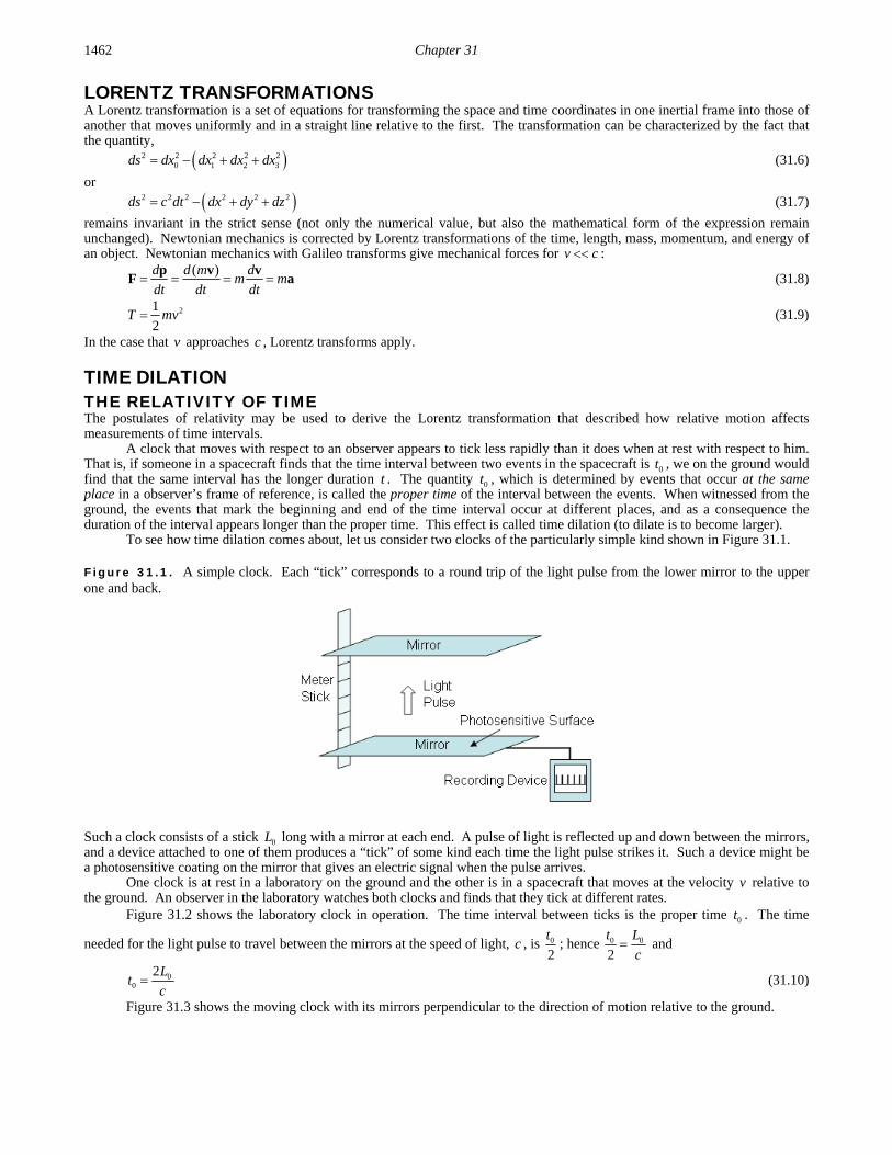
Chapter 31 1462
LORENTZ TRANSFORMATIONS A Lorentz transformation is a set of equations for transforming the space and time coordinates in one inertial frame into those of another that moves uniformly and in a straight line relative to the first. The transformation can be characterized by the fact that the quantity,
2 2 2 2 20 1 2 3ds dx dx dx dx (31.6)
or
2 2 2 2 2 2ds c dt dx dy dz (31.7)
remains invariant in the strict sense (not only the numerical value, but also the mathematical form of the expression remain unchanged). Newtonian mechanics is corrected by Lorentz transformations of the time, length, mass, momentum, and energy of an object. Newtonian mechanics with Galileo transforms give mechanical forces for v c :
( )d d m d
m mdt dt dt
p v v
F a (31.8)
21
2T mv (31.9)
In the case that v approaches c , Lorentz transforms apply. TIME DILATION THE RELATIVITY OF TIME The postulates of relativity may be used to derive the Lorentz transformation that described how relative motion affects measurements of time intervals.
A clock that moves with respect to an observer appears to tick less rapidly than it does when at rest with respect to him. That is, if someone in a spacecraft finds that the time interval between two events in the spacecraft is 0t , we on the ground would find that the same interval has the longer duration t . The quantity 0t , which is determined by events that occur at the same place in a observer’s frame of reference, is called the proper time of the interval between the events. When witnessed from the ground, the events that mark the beginning and end of the time interval occur at different places, and as a consequence the duration of the interval appears longer than the proper time. This effect is called time dilation (to dilate is to become larger).
To see how time dilation comes about, let us consider two clocks of the particularly simple kind shown in Figure 31.1.
Figure 31.1. A simple clock. Each “tick” corresponds to a round trip of the light pulse from the lower mirror to the upper one and back.
Such a clock consists of a stick 0L long with a mirror at each end. A pulse of light is reflected up and down between the mirrors, and a device attached to one of them produces a “tick” of some kind each time the light pulse strikes it. Such a device might be a photosensitive coating on the mirror that gives an electric signal when the pulse arrives.
One clock is at rest in a laboratory on the ground and the other is in a spacecraft that moves at the velocity v relative to the ground. An observer in the laboratory watches both clocks and finds that they tick at different rates.
Figure 31.2 shows the laboratory clock in operation. The time interval between ticks is the proper time 0t . The time
needed for the light pulse to travel between the mirrors at the speed of light, c , is 0
2
t; hence 0 0
2
t L
c and
00
2Lt
c (31.10)
Figure 31.3 shows the moving clock with its mirrors perpendicular to the direction of motion relative to the ground.

Relativity 1463
Figure 31.2. A light-pulse clock at rest on the ground as seen by an observer on the ground. The dial represents a conventional clock on the ground.
The time interval between ticks is t. Because the clock is moving, the light pulse, as seen from the ground, follows a
zigzag path. On its way from the lower mirror to the upper one in the time 2
t, the pulse travels a horizontal distance of
2
tv and
a total distance of 2
tc . Since 0L is the vertical distance between the mirrors,
2 2
202 2
t tc L v
(31.11)
2
2 2 204
tc v L (31.12)
22
02 02 2 2
22
24
1
LLt
c v vc
c
(31.13)
0
2
2
2
1
L
ctvc
(31.14)
But 02L
c is the time interval 0t between ticks on the clock on the ground, as in Eq. (31.10), and so the time dilation
relationship is:
0
2
21
tt
vc
(31.15)
wherein the parameters are:
0t = time interval on clock at rest relative to an observer
t = time interval on clock in motion relative to an observer v = speed of relative motion c = speed of light
Because the quantity 2
21
v
c is always smaller than 1 for a moving object, t is always greater than 0t . The moving clock
in the spacecraft appears to tick at a slower rate than the stationary one on the ground, as seen by an observer on the ground. Exactly the same analysis holds for measurements of the clock on the ground by the pilot of the spacecraft. To him, the
light pulse of the ground clock follows a zigzag path that requires a total time t per round trip. His own clock, at rest in the spacecraft, ticks at intervals of 0t . He too finds that
Figure 31.3. A light-pulse clock in a spacecraft as seen by an observer on the ground. The mirrors are parallel to the direction of motion of the spacecraft. The dial represents a conventional clock on the ground.

Chapter 31 1464
0
2
21
tt
vc
(31.16)
so the effect is reciprocal: Every observer finds that clocks in motion relative to him tick more slowly than clocks at rest relative to him.
The Lorentz transformation of time, length, mass, momentum, and energy which are significant when v approaches c can be derived by a similar procedure [2]. The Lorentz transformations are:
0
2
21
tt
vc
(31.17)
2
21o
vl l
c (31.18)
0
2
21
mm
vc
(31.19)
0
2
21
m vp
vc
(31.20)
2
2 0
2
21
m cE mc
vc
(31.21)
2 2 4 2 20E m c p c (31.22)
When speaking of the relativity of a frame of reference or simply of relativity, one usually means that there exist identical physical processes in different frames of reference. According to the generalized Galilean principle of relativity identical processes are possible in all inertial frames of reference related by Lorentz transformations. On the other hand, Lorentz transformations characterize the uniformity of Galilean spacetime. THE RELATIVITY PRINCIPLE AND THE COVARIANCE OF EQUATIONS IN GALILEAN OR EUCLIDEAN SPACETIME AND RIEMANN SPACETIME From the geometrical point of view the theory of space and time naturally divides into the theory of uniform, Galilean, space and the theory of non-uniform, Riemannian, space.
Galilean space is of maximal uniformity. This means that in it:
(a) All points in space and instants in time are equivalent
(b) All directions are equivalent, and
(c) All inertial systems, moving uniformly and in a straight line relative to one another, are equivalent (Galilean principle of relativity).
The uniformity of space and time manifests itself in the existence of a group of transformations which leave the four-dimensional interval between two points (distance) invariant. The expression for this interval plays an important part in the theory of space and time because its form is directly related to the form taken by the basic laws of physics, viz. the law of motion of a free mass-point and the law of propagation in free space of the front of a light wave.
The indications (a), (b) and (c) of the uniformity of Galilean space are related to the following transformations: (a) To the equivalence of all points and instants corresponds to the transformation of displacing the origins of the
spatial coordinates and of time; the transformation involves four parameters, namely, the three space coordinates and the time coordinate of the origin.
(b) To the equivalence of all directions corresponds to the transformation of rotating the spatial coordinate axes; this involves three parameters, the three angles of rotation.
(c) To the equivalence of inertial frames corresponds to a change from one frame of reference to another moving uniformly in a straight line with respect to the first; this transformation involves three parameters, the three components of relative velocity.
The most general transformation involves ten parameters. This is the Lorentz transformation. It is well known that in a space of n dimensions the group of transformations which leave invariant the expression for the squared distance between
infinitely near points, can contain at most 11
2n n parameters. If there is a group involving all 1
12
n n parameters then the

Relativity 1465
space is of maximal uniformity; it may be a space of constant curvature, or, if the curvature vanishes, a Euclidean or pseudo-Euclidean space.
In the case of spacetime, the number of dimensions is four and therefore the greatest possible number of parameters is ten. This is also the number of parameters in the Lorentz transformation, so that Galilean space, to which the transformation relates, is indeed of maximal uniformity. It is customary to call the theory based on the Lorentz transformations the special theory of relativity. More precisely, the subject of that theory is the formulation of physical laws in accordance with the properties of Galilean space.
A formulation of the principle of relativity given supra, which together with the postulate that the velocity of light has a limiting character, may be made the basis of relativity theory. We shall now investigate in more detail the question of the connection of the physical principle of relativity with the requirement that the equations be covariant.
In the first place, we shall attempt to give a generally covariant formulation of the principle of relativity, without as yet making this concept more precise. In its most general form, the principle of relativity states the equivalence of the coordinate systems (or frames of reference) that belong to a certain class and are related by transformations of the form: 0 1 2 3' , , ,x f x x x x (31.23)
which may be stated more briefly as: 'x f x (31.24)
It is essential to remember that, in addition to the group of permissible transformations, the class of coordinate systems must be characterized by certain supplementary conditions. Thus, for instance, if we consider Lorentz transformations, it is self-evident that these linear transformations must connect not any arbitrary coordinates, but only the Galilean coordinates in two inertial reference frames. To consider linear transformations between any other (non-Galilean) coordinates has no sense, because the Galilean principle of relativity has no validity in relation to such artificial linear transformations. On the other hand, if one introduces any other variables in place of the Galilean coordinates, a Lorentz transformation can evidently be expressed in terms of these variables, but then the transformation formulae will have a more complicated form.
The formulation of the principle of relativity based on the equivalence of reference frames depends on the ability to call two reference frames x and 'x physically equivalent if phenomena proceed in the same way in them. Specifically, if a possible process is described in the coordinates x by the functions: 1 2, , ..., nx x x (31.25)
then there is another possible process which is describable by the same functions 1 2' , ' , ..., 'nx x x (31.26)
in the coordinates 'x . Conversely any process of the form Eq. (31.26) in the second system corresponds to a possible process of the form Eq. (31.25) in the first system. Thus, a relativity principle is a statement concerning the existence of corresponding processes in a set of reference frames of a certain class wherein the corresponding systems are accepted as equivalent. It is clear from this definition that both the principle of relativity itself and the equivalence of two reference frames are physical concepts, and validity of either involves a definite physical hypothesis rather than convention. In addition, it follows that the very notion of a “principle of relativity” becomes well defined only when a definite class of frames of reference has been singled out. In the usual theory of relativity, this class is that of inertial systems.
The functions Eq. (31.25) or Eq. (31.26) describing a physical process will be called field functions or functions of state. In a generally covariant formulation of the equations describing physical processes the components g of the metric tensor must be included among the functions of state such as the collection of field functions: , ,F x j x g x (31.27)
i.e. the electromagnetic field, the current vector, and the metric tensor, respectively. The requirement for the formulation of a principle of relativity that in two equivalent reference frames corresponding phenomena should proceed in the same way applies equally to the metric tensor. Thus, if we compare two corresponding phenomena in to physically equivalent reference frames, then for the first phenomenon, described in the old coordinates, not only the components of electromagnetic field and of current density, but also the components of the metric tensor must have the same mathematical form as for the second phenomenon described in the new coordinates.
Further conclusions depend on whether the metric is assumed to be fixed or whether phenomena that influence the metric are considered. In the usual theory of relativity, it is assumed that the metric is given, and it does not depend on any physical processes. This is also the case for the generally covariant formulation of the theory of relativity. As long as the assumption remains in force that the character of spacetime is Galilean and the g are introduced only to achieve general covariance, these quantities will depend only on the choice of coordinate system, not on the nature of the physical process discussed. They are functions of state only in a formula sense. In the theory of gravitation on the other hand, a different assumption is made concerning the nature of spacetime. There the g are functions of state, not only in a formal sense, but in fact: they describe a certain physical field, namely the field of gravitation.
To give a definite meaning to the principle of relativity in such circumstances, it is essential to specify more closely not only the class of coordinate systems, but also the nature of the physical processes for which the principle is being formulated. Starting from the assumption that the metric is fixed (“rigid”), or that it may be considered as fixed for a certain class of physical processes, consider the above definition of corresponding phenomena in two physically equivalent coordinate systems, wherein all field functions, including the components of the metric tensor, must have the same mathematical form for the first process described in the old coordinates as for the second process described in the new coordinates. If the g are independent of the nature of the physical phenomenon, then a distinction must be made between the first and second process relative to those quantities, and only transformations of the coordinates need to be considered. Thus, the quantities

Chapter 31 1466
g x and ' 'g x (31.28)
will be connected by the tensor transformation rule, and the requirement of the relativity principle that they should have one and the same mathematical form reduces (for infinitesimal coordinate transformations) to the equations 0g .
The most general class of transformations that satisfies these equations contains 10 parameters and is possible only in uniform spacetime, where the relation, , ( )R K g g g g (31.29)
is valid. (A space in which the curvature tensor ,R has the form of Eq. (31.29) is called a space of constant curvature; it is a
four-dimensional generalization of Friedmann-Lobachevsky space. The constant K is called the constant of curvature.) If in these relations, K is zero, the spacetime is Galilean and the transformations in questions are Lorentz transformations, except when other (non-Galilean) coordinates are used.
Thus, with the rigidity assumption for the metric, the principle of relativity implies the uniformity of spacetime. And, if the additional condition 0K holds, we obtain a Galilean metric in appropriate coordinates. The relativity principle in general form then reduces to the Galilean relativity principle. As for the condition 0K , it results in an additional uniformity of spacetime. If the scale of the Galilean coordinates is changed, then the scale of the elementary interval changes in the same proportion. This property implies in turn that there is no absolute scale for spacetime, unlike the absolute scale that exists for velocities in terms of the velocity of light. The absence of an absolute scale for spacetime leads conversely to the equation
0K . Furthermore, taking into account phenomena that may influence the metric gives rise to the possibility that under certain
conditions the principle of relativity will be valid in non-uniform space also. In this case, it is necessary that the motion of the masses producing the non-uniformity be included in the description of the phenomena.
It can be shown that under the assumption that spacetime is uniform at infinity (where it must be Galilean), a class of coordinate systems exist that are analogous to inertial systems and defined up to a Lorentz transformation. A principle of relativity will hold with respect to this class of coordinate systems in the same form as in the usual theory of relativity, despite the fact that at a finite distance from the masses the space is non-uniform. However, ultimately, this relativity principle is also a result of uniformity forced by the boundary conditions that require uniformity at infinity.
Since the greatest possible uniformity is expressed by Lorentz transformations, there is no more general principle of relativity than that discussed in ordinary relativity theory. Moreover, there cannot be a general principle of relativity, as a physical principle, which would hold with respect to arbitrary frames of reference. In order to make this fact clear, it is essential to distinguish sharply between a physical principle that postulates the existence of corresponding phenomena in different frames of reference and the simple requirement that equations should be covariant transforming from one frame of reference to another. It is clear that a principle of relativity implies a covariance of equations, but the converse is not true: covariance of differential equations is also possible when no principle of relativity is satisfied.
Covariance of equations in itself is in no way the expression of any kind of physical law. For instance, consider the mechanics of systems of mass-points. Lagrange’s equations of the second kind are covariant with respect to arbitrary transformations of the coordinates. However, they do not express any new physical law compared to, for example, Lagrange’s equations of the first kind, which are stated in Cartesian coordinates and are not covariant. In the case of Lagrange’s equations, covariance is achieved by introducing the coefficients of the Lagrangian as new auxiliary functions considered as a quadratic expression, but not necessarily homogeneous in the velocities.
Independently considering that not all laws of nature reduce to differential equations, even fields described by differential equations not only require these equations for their definitions, but also all kinds of initial, boundary, and other conditions. These conditions are not covariant. Therefore, the preservation of their physical content requires a change in their mathematical form and, conversely, preservation of their mathematical form implies a change of their physical content. But, the realization of a process with a new physical content is an independent question that cannot be solved a priori. If “corresponding” physical processes within a given class of reference systems are possible, then a principle of relativity holds. In the opposite case, it does not. It is clear, however, that such a model representative of physical processes, and in particular such a model representative of the metric, is possible at most for a narrow class of reference systems of limited number. This argument shows once again (without invoking the concept of uniformity) that a general principle of relativity, as a physical principle, holding in relation to arbitrary frames of reference, is impossible.
A desire to find a general principle of relativity is unnecessary as a basis of the requirement of the covariance of the equations. The covariance requirement can be justified independently. It is a self-evident, purely logical requirement that in all cases in which the coordinate system is not fixed in advance, equations written down in different coordinate systems should be mathematically equivalent. The class of transformations with respect to which the equations must be covariant must correspond to the class of coordinate systems considered. Thus, if one deals with inertial systems related by Lorentz transformations and if Galilean coordinates are used, it is sufficient to require covariance with respect to Lorentz transformations. If, however, arbitrary coordinates are employed, it is necessary to demand general covariance.
It should be noted that covariance of coordinate systems acquires definite physical meaning if, and only if, a principle of relativity exists for the class of reference frames used. Such is the covariance with respect to Lorentz transformations. This concept was so useful in the formulation of physical laws because it contains concrete temporal and geometric elements (rectilinearity and uniformity of motion) and also dynamic elements (the concept of inertia in the mechanical and the electromagnetic sense). Because of this, it is related to the physical principle of relativity and itself becomes concrete and physical.

Relativity 1467
However, if arbitrary transformations are considered rather than the Lorentz transformations, one ceases to single out that class of coordinate systems relative to which the principle of relativity exists, and by doing this one destroys the connection between physics and the concept of covariance. There remains a purely logical side to the concept of covariance as a consistency requirement on equations written in different coordinate systems. Naturally this requirement is necessary, and it can always be satisfied.
In dealing with classes of reference frames that are more general than that relative to which a principle of relativity holds, the necessity arises of replacing the explicit formulation of the principle by some other statement. The explicit formulation consists of indicating a class of physically equivalent frames of reference. The new formulation must express those properties of space and time by which the principle of relativity is possible. With the assumption of a rigid metric this is achieved by introducing an additional Eq. (31.29). With the additional assumption of the absence of a universal scale ( 0K ) these equations lead to a generally covariant formulation of the theory of relativity, without any alteration of its physical content. The Galileo-Lorentz principle of relativity is then maintained to its full extent.
The very possibility of formulating the ordinary theory of relativity in a general covariant form clearly demonstrates the difference between the principle of relativity as a physical principle and the covariance of the equations as a logical requirement. In addition, such a formulation opens the way to generalizations based on a relaxation of the assumption of a rigid metric. This relaxation provides the possibility of replacing the supplementary conditions Eq. (31.29) by others that reflect better the properties of space and time corresponding to the theory of gravitation.
Universal gravitation does not fit into the framework of uniform Galilean space because the gravitational mass of a body as well as the inertial mass depends on its energy. In the latter case, Einstein felt that it was possible to eliminate the effects of gravity by transforming to an accelerating frame of reference that defined his “Equivalence Principle.” A theory of universal gravitation is derived in the Gravity section wherein Euclidean, or rather pseudo-Euclidean, geometry is abandoned in favor of the geometry of Riemann. But the derivation does not involve the traditional approach based on the Equivalence Principle; rather it is based on Eq. (31.2).
In Riemannian geometry, the coefficients g of the quadratic form for the squared infinitesimal distance are mechanics
functions. These functions establish a law regarding their transformation from one coordinate frame to another based on their definition as coefficients of a quadratic form, together with the condition that this form is an invariant. Thus, a transformation of the coordinates is accompanied by a transformation of the metric g according to this law. The set of quantities g is called
the metric tensor. With the introduction of a metric tensor, expressions can be formed that are covariant with respect to any coordinate
transformation. Nothing other than the covariance of equations is implicit in the metric tensors that may be obtainable from a particular one (e.g. from the Galilean tensor) by coordinate transformation. But, metric tensors of a more general form that cannot be transformed into one another by coordinate transformations are fundamentally different. In each case, the metric tensor will express not only properties of the coordinate system but also properties of space, and the latter can be related to the phenomenon of gravitation. It is shown below that the origin of gravity is the relativistic correction of spacetime itself as opposed to the relativistic correction of mass, length, and time of objects of inertial frames in constant relative motion. The production of a particle having an inertial and gravitational mass from a photon traveling at the speed of light requires time dilation and length contraction of spacetime. The present theory of gravity also maintains the constant maximum speed of light for the propagation of any form of energy including the gravitational field.
Having clarified the concept of covariance as applied to Riemannian geometry, consider it together with the previously discussed concept of the uniformity of space. As was shown above, the property of uniformity in Galilean space manifests itself in the existence of transformations that leave unchanged the expression for the four-dimensional distance between two points. More precisely, these transformations leave unchanged the coefficients of this expression, i.e. the quantities g . g are
functions of the coordinates which means that the mathematical form of these functions is unchanged: The dependence of the new g on the new coordinates has the same mathematical form as that of the old g on the old coordinates. In the general
case of Riemannian geometry, there are no transformations that leave the g unchanged because Riemannian space is not
uniform. One deals with transformations of coordinates accompanied by transformations of the g , and neither such a
combined transformation nor covariance with respect to it has any relation to the uniformity or non-uniformity of space. The geometrical properties of real physical space and time correspond not to Euclidean but to Riemannian geometry.
Any deviation of geometrical properties from their Euclidean, or to be precise, pseudo-Euclidean form appears in Nature as a gravitational field. The geometrical properties are inseparably linked with the distribution and motion of ponderable matter. This relationship is mutual. On the one hand the deviations of geometrical properties from the Euclidean are determined by the presence of gravitating masses, on the other, the motion of masses in the gravitational field is determined by these deviations. In short, masses determine the geometrical properties of space and time, and these properties determine the movement of the masses. The description of the gravitational field demands the introduction of no functions other than the metric tensor itself which is uniquely determined by the presence and motion of matter. Differing from other kinds of forces, gravity which influences the motion of the matter by determining the properties of spacetime, is itself described by the metric of spacetime. For this principle of relativity, the class of coordinate systems relative to which the principle of relativity exists is the spherical coordinate systems. Spherical harmonic coordinates arise naturally due to the spherical symmetry of the particle production (energy/matter conversion) event and its effect on spacetime and provide the connection between physics and the concept of covariance as shown in the Gravity section. The corresponding metric is the Schwarzschild metric derived in the Gravity section.

Chapter 31 1468
The Schwarzschild metric gives the relationship whereby matter causes relativistic corrections to spacetime that determines the curvature of spacetime and is the origin of gravity. The correction is based on the boundary conditions that no signal can travel faster that the speed of light including the gravitational field that propagates following particle production from a photon wherein the particle has a finite gravitational velocity given by Newton’s Law of Gravitation. The spacetime contraction during particle production is analogous to Lorentz length contraction and time dilation of an object in one inertial frame relative to another moving at constant relative velocity. In the former case, the corresponding correction is a function of the square of the ratio of the gravitational velocity to the speed of light. In the latter case, the corresponding correction is a function of the square of the ratio of the relative velocity of two inertial frames to the speed of light. Thus, the relativity principle for both Euclidean and Riemannian geometries is based on the light wave front propagation equation, specifically Eq. (31.2).
REFERENCES 1. S. Kak, “Moving observers in an isotropic universe,” International Journal of Theoretical Physics, Vol. 46, (2007). 2. A. Beiser, Concepts of Modern Physics, Fourth Edition, McGraw-Hill Book Company, New York, (1978), pp. 2-40. 3. V. Fock, The Theory of Space, Time, and Gravitation, The MacMillan Company, (1964). 4. J. Bailey et al., “Final report on the CERN muon storage ring including the anomalous magnetic moment and the electric
dipole moment of the muon, and a direct test of relativistic time dilation, Nuclear Physics B150, (1979), pp. 1-75. 5. P. Sprangle, A. T. Drobot, “The linear and self-consistent nonlinear theory of the electron cyclotron maser instability,” IEEE
Transactions on Microwave Theory and Techniques, Vol. MTT-25, No. 6, June, (1977), pp. 528-544. 6. E. Giannetto, The rise of special relativity: Henri Poincaré’s works before Einstein. Atti del 18 Congresso di Storia della
Fisica e dell’Astronomia, (1998). 7. H. Poincaré, “L’etat actuel et l’avenir de la physique mathematique,” Bulletin des sciences mathematiques, Vol. 28, (1904),
pp. 302-324; quoted in Whittaker (1987), p. 30. 8. E. Whittaker, A History of the Theories of Aether and Electricity, Vol. 2, Modern Theories, Chapter 2, “The Relativity
Theories of Poincaré and Lorentz,” Nelson, London, (1987), Reprinted, American Institute of Physics, pp. 30–31.

1469
Chapter 32 GRAVITY
QUANTUM GRAVITY OF FUNDAMENTAL PARTICLES The attractive gravitational force has been the subject of investigation for centuries. Traditionally, gravitational attraction has been investigated in the field of astrophysics applying a large-scale perspective of cosmological spacetime, as distinguished from currently held theories of atomic and subatomic structure. However, gravity originates on the atomic scale. In Newtonian gravitation, the mutual attraction between two particles of masses 1m and 2m separated by a distance r is:
1 22
m mG
rF (32.1)
where G is the gravitational constant, its value being 11 2 2 6.67 10X Nm kg . Although Newton’s theory gives a correct
quantitative description of the gravitational force, the most elementary feature of gravitation is still not well defined. What is the most important feature of gravitation in terms of fundamental principles? By comparing Newton’s second law, mF a (32.2) with his law of gravitation, we can describe the motion of a freely falling object by using the following equation:
3i g
GMm m
ra r (32.3)
where im and gm represent respectively the object’s inertial mass (inversely proportional to acceleration) and the gravitational
mass (directly proportional to gravitational force), M is the gravitational mass of the Earth, and r is the position vector of the
object taken from the center of the Earth. The above equation can be rewritten as:
2
a g
i
m GM
m r
(32.4)
Extensive experimentation dating from Galileo Galilei’s Pisa experiment to the present has shown that irrespective of the object chosen, the acceleration of an object produced by the gravitational force is the same, which from Eq. (32.4) implies that the value of /g im m should be the same for all objects. In other words, we have
universal constantg
i
m
m (32.5)
the equivalence of the gravitational mass and the inertial mass. The fractional deviation of Eq. (32.5) from a constant is experimentally confirmed to less 111 10X [1]. In physics, the discovery of a universal constant often leads to the development of an entirely new theory. From the universal constancy of the velocity of light, c, the special theory of relativity was derived; and from Planck’s constant, h, the quantum theory was deduced. Therefore, the universal constant /g im m should be the key to
the gravitational problem. The theoretical difficulty with Newtonian gravitation is to explain just why relation, Eq. (32.5), exists implicitly in Newton’s theory as a separate law of nature besides Eqs. (32.1) and (32.2). Furthermore, discrepancies between certain astronomical observations and predictions based on Newtonian celestial mechanics exist, and they apparently could not be reconciled until the development of Einstein’s theory of general relativity which can be transformed to Newtonian gravitation on the scale in which Newton’s theory holds.
General relativity is the geometric theory of gravitation developed by Albert Einstein, whereby he intended to incorporate and extend the special theory of relativity to accelerated frames of reference. Einstein’s theory of general relativity is based on a flawed dynamic formulation of Galileo Galilei’s law. Einstein took as the basis to postulate his gravitational field equations a certain kinematical consequence of a law, which he called the “Principle of Equivalence,” which states that it is impossible to

Chapter 32 1470
distinguish a uniform gravitational field from an accelerated frame. However, the two are not equivalent since they obviously depend on the direction of acceleration relative to the gravitating body and the distance from the gravitating body since the gravitational force is a central force. (In the latter case, only a line of a massive body may be exactly radial, not the entire mass.) And, this assumption leads to conflicts with special relativity. The success of Einstein’s gravity equation can be traced to a successful solution which arises from assumptions and approximations whereby the form of the solution ultimately conflicts with the properties of the original equation; no solution is consistent with the experimental data in the case of the possible cosmological solutions of Einstein’s general relativity. Furthermore, Einstein’s general relativity is a partial theory in that it deals with matter on the scale of celestial objects, but not on an atomic scale. And, it fails on the cosmological scale. All gravitating bodies are composed of matter and are collections of atoms that are composed of fundamental particles such as electrons, which are leptons, and quarks, which make up protons and neutrons. Gravity originates from the fundamental particles.
Einstein’s theory has as its foundation that gravity is a force unique from electromagnetism. The magnetic force was unified with the Coulomb force by Maxwell. Lorentz derived the transformations named after him which formalize the origin of the magnetic force as a relativistic correction of the Coulomb force. The unification of electricity and magnetism by Maxwell permitted him to derive a wave equation that predicted the propagation of electromagnetic waves at the speed of light. Maxwell’s wave equation defines a four-dimensional spacetime and the speed of light as a maximum permitted according to the permeability and permittivity of spacetime. Minkowski originated the concept of a four-dimensional spacetime formally expressed as the Minkowski tensor [2]. The Minkowski tensor corresponds to the electromagnetic wave equation derived by Maxwell and can be derived from it [3]. Special relativity is implicit in the wave equation of electromagnetic waves that travel at the speed of light. As given in the Relativity section and the Equivalence of Inertial and Gravitational Masses Due to Absolute Space and Absolute Light Velocity section, the generalization of this metric to mass as well as charge requiring application of Lorentz transformations comprises the theory of special relativity invented by Poincaré in 1904 [4-6]1. The Lorentz transformations quantify the measurement of the increase in mass, length contraction, and time dilation in the direction of constant relative motion of separate inertial frames due to the finite maximum speed of light. The goal of Einstein, who worked on special relativity, was to generalize it to accelerated frames of reference as well as inertial frames moving at constant relative velocity. But, gravity is not a force separable from electromagnetism. The true origin of gravity is the relativistic correction of spacetime itself as opposed to the relativistic correction of mass, length, and time of objects of inertial frames in constant relative motion. The production of a massive particle from a photon with zero rest mass traveling at the speed of light requires time dilation and length contraction of spacetime. The present theory of gravity also maintains the constant maximum speed of light for the propagation of any form of energy. (Recently the speed of gravity has been measured to be the speed of light [7].) And, the origin of the gravitational force is also a relativistic correction. In the metric which arises due to the presence of mass, spacetime itself must be relativistically corrected as a consequence of the presence of mass in order that (i) the speed of light is constant and a maximum, (ii) the angular momentum of a photon, , is conserved, and (iii) the energy of the photon is conserved as mass. Spacetime must undergo time dilation and length contraction due to the production event. The event must be spacelike even though the photon of the particle production event travels at the speed of light and the particle must travel at a velocity less than the speed of light. The relativistically altered spacetime gives rise to a gravitational force between separated masses. Thus, the production of matter and its motion alters spacetime and the altered spacetime affects the motion of matter, which must follow geodesics.
When speaking of the relativity of a frame of reference or simply of relativity, one usually means that there exist identical physical processes in different frames of reference. According to the generalized Galilean principle of relativity identical processes are possible in all inertial frames of reference related by Lorentz transformations. On the other hand, Lorentz transformations characterize the uniformity of Galilean spacetime. Using the four-dimensional coordinates x for describing the events and the world-line in spacetime the separation of proper time between two events x and x dx is: 2d g dx dx
(32.6)
where g is the metric tensor which determines the geometric character of spacetime. For different coordinate systems, the
dx may not be the same, but the separation 2d remains unchanged. The metric g for Euclidean space called the
Minkowski tensor is:
1 In 1900, Lorentz conjectured that gravitation could be attributed to actions that propagate with the velocity of light. Poincaré, in a paper in July 1905 (submitted days before Einstein’s special relativity paper), suggested that all forces should transform according to Lorentz transformations. In this case, he notes that Newton’s Law of Gravitation is not valid and proposed gravitational waves that propagated with the velocity of light. Specifically, Poincaré pointed out that all forces must propagate with the finite light velocity, that interaction implies a time delay, and it is mediated by field waves. Thus, Poincaré made for the first time the hypothesis of the existence of gravitational waves [4].

Gravity 1471
2
2
2
1 0 0 0
10 0 0
10 0 0
10 0 0
c
c
c
(32.7)
In this case, the separation of proper time between two events x and x dx is: 2d dx dx
(32.8)
A spherically symmetrical system of mass 0m applies to the production of a particle which implies spherical coordinates
with the origin at 0. Thus, a family of curved surfaces, each with constant r, is a series of concentric spheres on which it is natural to adopt the coordinate r so that a sphere with constant r has area 24 r , and the metric on the surface of the sphere would then be: 2 2 2 2 2 2sinds r d r d (32.9) Such a definition of r is no longer the distance from the origin to the surface, because of the spacetime contraction caused by the mass 0m . The form of the outgoing gravitational field front traveling at the speed of light is:
r
f tc
(32.10)
Therefore the spatial metric should be expressed as
12 2 2 2 2 2 2sinds f r dr r d r d (32.11)
In addition, the existence of mass 0m also causes time dilation of spacetime such that the clock on each r-sphere is no
longer observed from each r-sphere to run at the same rate. That is, clocks slow down in a gravitational field [8]. Therefore, the general form of the metric due to the relativistic effect on spacetime due to mass 0m is:
12 2 2 2 2 2 2 22
1sind f r dt f r dr r d r d
c (32.12)
In the case where 0 0m , space would be flat which corresponds to:
11f r f r
(32.13)
Then the spacetime metric is the Minkowski tensor. In the case that the mass 0m is finite, the Minkowski tensor is corrected by
the time dilation and length contraction of spacetime. The creation of a particle from light requires the event to be spacelike; yet, particle production arises from a photon
traveling at the speed of light. At production, the particle must have a finite velocity called the Newtonian gravitational velocity (according to Newton’s Law of Gravitation) that may not exceed the speed of light. The Newtonian gravitational velocity must have an associated gravitational energy. The photon initially traveling at the speed of light undergoes particle production and must produce a gravitational field that travels at the speed of light. The gravitational energy associated with the field must have an inverse radius dependence according to the spreading wave. Since the gradient of the gravitational energy gives rise to the gravitational field, the gravitational field must have an inverse radius squared dependence. In order that the velocity of light does not exceed c in any frame including that of the particle having a finite Newtonian gravitational velocity, gv , the laboratory
frame of an incident photon, and that of a gravitational field propagating outward at the speed of light, spacetime must undergo time dilation and length contraction due to the production event. During particle production the speed of light as a constant maximum as well as phase matching and continuity conditions require the following form of the squared displacements due to constant motion along two orthogonal axes in polar coordinates:
22 2
gc v t ct (32.14)
22 2
gc ct v t (32.15)
2
2 2 1 gvt
c
(32.16)
Thus,
2
1 gvf r
c
(32.17)

Chapter 32 1472
(The derivation and result of spacetime time dilation is analogous to the derivation and result of special relativistic time dilation given by Eqs. (30.11-30.15).) Therefore, the general form of the metric due to the relativistic effect on spacetime due to mass
02 2 2
1 1 10 0 0 0 02
proper time
coordinate time 2 2 2C G G
u C
Gm
m e c e c Gm e c v v
m h c h c h c c
is:
12 2
2 2 2 2 2 2 2 22
11 1 sing gv v
d dt dr r d r dc c c
(32.18)
The gravitational energy of a particle during production given by Newton’s Law of Gravitation may be unified with the inertial and electromagnetic energies given by Planck’s equation and Maxwell’s equations, respectively. The physical basis is the law of Galileo that in the absence of a resistive medium all bodies fall equally fast, or, more accurately, with equal acceleration. The law of Galileo can be stated in generalized form as the law of the equality of inertial and gravitational mass. The equivalence of the Planck equation, electric potential, and the stored magnetic energies occurs for a transition state atomic orbital during pair production as shown in the Pair Production section. During particle production the transition state atomic orbital has a charge-density function given by
2( )
4 n
er r
r
(32.19)
where e is the fundamental charge. The corresponding mass-density function is:
02
( )4 n
mr r
r
(32.20)
where mass, 0m , is the rest mass of the particle produced. In both cases, the radius, nr , is the Compton wavelength bar, C ,
given by
*
0C r
m c (32.21)
Consider the gravitational radius, G or Gr , of an atomic orbital of mass, 0m , defined as:
02G G
Gmr
c (32.22)
where G is the Newtonian gravitational constant. Notice that as 0m increases the gravitational radius, Gr , increases (i.e. the
curvature of spacetime increases), and the radius of the transition state atomic orbital, *r , decreases. Remarkably, when *
G Cr r , the gravitational potential energy equals 20m c where 0m is the rest mass of the fundamental particle created as the
transition state atomic orbital becomes real. This is shown by equating the gravitational radius, Gr , to the Compton wavelength
bar, C , given by Eq. (29.22):
02
0c
Gm
c m c
(32.23)
Multiplication of both sides of Eq. (32.23) by 20m c and division of both sides by * gives:
20
* *
Gm c
(32.24)
Since / 2h :
20
* *
2
Gm hc
(32.25)
Since / 2C C and from Eqs. (27.3) and (27.5), *
hc
:
2 2
*0 0*
C
Gm Gm
r
(32.26)
The left-hand side of Eq. (32.26) is the gravitational potential energy and the right-hand side is the energy of the particle-production photon. Thus, from Eq. (28.11) and Eq. (32.26), the following energies are equivalent
2
2 * 00 *mag
C
GmE m c V E
(32.27)
where * is the angular frequency of the photon which forms the transition state atomic orbital, and * is also the spacetime resonance angular frequency for this particle. Furthermore, given

Gravity 1473
2 *0 *
hcE m c
(32.28)
It follows that
*
0 0
h h h
m c m v p (32.29a)
and in general,
h h
mv p (32.29b)
This equation is the de Broglie relationship; it must hold for matter and energy. In fact, this was de Broglie’s original insight [9] which led him to postulate the relationship named after him. The mass-energy which causes the gravitational radius, Gr , to
equal C is hereafter called the Grand Unification Mass-Energy which is equal to times the angular frequency of the photon
which becomes the transition state atomic orbital. This angular frequency is also the spacetime resonance angular frequency of the Grand Unification Mass-Energy as given by Eq. (28.13). The Grand Unification Mass-Energy is further equal to the corresponding electric potential, stored magnetic, and gravitational potential energy. The equality of radii unifies de Broglie’s equation, Planck’s equation, Maxwell’s equations, Newton’s equations, and Special and General Relativity, which comprise the fundamental laws of the Universe.
The Grand Unification Mass-Energy, um , can be expressed in terms of Planck’s constant.
2
2 2*
u uu u
C
Gm m cm c Gm
(32.30)
u
cm
G
(32.31)
The Grand Unification Mass-Energy, um , given by Eq. (32.31) is the Planck mass. From Eq. (28.11), the relationship of the
equivalent particle production energies (mass energy = Planck equation energy = electric potential energy = magnetic energy = gravitational potential energy) is 2 *
0 mag gravm c V E E (32.32a)
where 0m is the rest mass of a fundamental particle of the Planck mass um when the gravitational energy is the gravitational
potential energy given by Eq. (32.30). A corresponding general relationship of the equivalent particle production energies (mass energy = Planck equation energy = electric potential energy = magnetic energy = gravitational energy) is:
2 2 2 22 22 * 1 1 10 0 0
0 22 30 0 0
4 22C C CC
e e c Gme cm c
m h Gm
(32.32b)
where 0m is the rest mass of a fundamental particle. For particle production, the gravitational velocity, Gv , is defined as
0 0G
C
Gm Gmv
r
(32.33)
Substitution of the gravitational velocity, Gv , given by Eq. (32.33) and the Planck mass, um , given by Eq. (32.31) into Eq.
(32.32) followed by division by the speed of light squared gives the mass of a fundamental particle in terms of the Planck mass where:
02 2 2
1 1 10 0 0 00 22 2 2
C G Gu u u u
C
Gm
e c e c Gm e c v vm m m m m
h c h c h c c
(32.34)
The equivalence of the gravitational and inertial masses according to experiments and Eq. (32.32) prove that Newton’s Gravitational Law is exact on a local scale. The production of a particle requires that the velocity of each of the point masses of the particle is equivalent to the Newtonian gravitational escape velocity gv of the superposition of the point masses of the
antiparticle. According to Newton’s Law of Gravitation the eccentricity is one (Eqs. (35.17-35.22)) and the particle production trajectory is a parabola relative to the center of mass of the antiparticle. The correction to Newton’s Gravitational Law due to the relativistic effect of the presence of mass on spacetime may be determined by substitution of the gravitational escape velocity,
gv , given by [10]:
0 02 2g
C
Gm Gmv
r
(32.35)
into Eq. (32.18) for gv . The corresponding Newtonian gravitational radius is given by:
02
2g
Gmr
c (32.36)

Chapter 32 1474
In the case of the boundary conditions of Eq. (32.32), Eq. (32.35) and Eq (32.36), three families of leptons and quarks are predicted wherein each particle corresponds to a unique atomic orbital radius equal to its Compton wavelength bar. At particle production, a photon having a radius and a wavelength equal to the Compton wavelength bar of the particle forms a transition state atomic orbital of the particle of the same wavelength.
A fourth family is not observed. A pair of particles each of the Planck mass corresponding to the conditions of Eq. (32.22), Eq. (32.32), and Eq. (32.33), is not observed since the velocity of each of the point masses of the transition state atomic orbital is the gravitational velocity Gv that in this case is the speed of light; whereas, the Newtonian gravitational escape velocity
gv of the superposition of the point masses of the antiparticle would be 2 the speed of light (Eq. (32.35)). In this case, an
electromagnetic wave of mass energy equivalent to the Planck mass travels in a circular orbit around the center of mass of another electromagnetic wave of mass energy equivalent to the Planck mass wherein the eccentricity is equal to zero (Eq. (35.21)), and the escape velocity can never be reached. The Planck mass is a “measuring stick.” The extraordinarily high
Planck mass ( 82.18 10 c
X kgG
) is the unobtainable mass bound imposed by the angular momentum and speed of the
photon relative to the gravitational constant. It is analogous to the unattainable bound of the speed of light for a particle possessing finite rest mass imposed by the Minkowski tensor. It has a physical significance for the fate of blackholes as given in the Composition of the Universe section.
Eq. (32.34) gives the relationship between the mass of each fundamental particle and the ratio of the gravitational velocity Gv to the speed of light times the Planck mass, the mass at which the gravitational radius Gr is the Compton wavelength
bar and the production energy is equal to the gravitational potential energy given by Eq. (32.30). The square of the ratio of the gravitational escape velocity gv of each particle relative to the speed of light gives the corresponding spacetime contraction
according to Eqs. (32.17-32.18). During particle production, a particle having the gravitational escape velocity gv is formed
from a photon traveling at the speed of light. The spacetime contraction during particle production is analogous to Lorentz length contraction and time dilation of an object in one inertial frame relative to another moving at constant relative velocity. In the latter case, the correction is the square of the ratio of the relative velocity of two inertial frames to the speed of light according to Eqs. (31.17-31.18). The theory of the masses of fundamental particles is given in the Particle Production section, the Leptons section, and The Quarks section.
The resulting metric is valid for the external region of particles and spherically symmetric bodies comprised of fundamental particles such as the celestial bodies. The metric g for non-Euclidean space due to the relativistic effect on
spacetime due to mass 0m is:
02
1
02 2
22
2 22
21 0 0 0
210 1 0 0
10 0 0
10 0 0 sin
Gm
c r
Gm
c c rg
rc
rc
(32.37)
In this case, the separation of proper time between two events x and x dx is:
1
2 2 2 2 2 2 2 20 02 2 2
2 211 1 sin
Gm Gmd dt dr r d r d
c r c c r
(32.38)
The origin of gravity is fundamental particles, and the masses and fields from particles superimpose. So, 0m , the mass of a
fundamental particle, may be replaced by M, the sum of the masses of the particles which make up a massive body. In this case, Eq. (32.38) is equivalent to a modified version of the Schwarzschild metric [8 and footnote 7].
One interpretation of the relativistic correction of spacetime due to conversion of energy into matter and matter into energy is that spacetime contracts and expands, respectively, in the radial and time dimensions. Thus, matter-energy conversion can be considered to conserve spacetime. Also, since matter causes spacetime to deviate from flat or Euclidean, matter-energy conversion can be considered to curve spacetime. The result is that spacetime is positively curved to match the boundary condition of the positive curvature of particles during production. The two-dimensional nature of fundamental particles requires that the radial and time dimensions are distinct from the angular dimensions. The curvature of spacetime results from a discontinuity of matter having curvature confined to two spatial dimensions. This is the property of all matter as an atomic orbital. A space in which the curvature tensor has the following form: , ( )R K g g g g (32.39)

Gravity 1475
is called a space of constant curvature; it is a four-dimensional generalization of Friedmann-Lobachevsky space. The constant K is called the constant of curvature. Consider an isolated atomic orbital and radial distances, r, from its center. For r less than nr
there is no mass; thus, spacetime is flat or Euclidean. The curvature tensor applies to all space of the inertial frame considered; thus, for r less than nr , 0K . At nr r there exists a discontinuity of mass of the atomic orbital. This results in a discontinuity
of the metric tensor for radial distances greater than or equal to nr which defines the curvature tensor given by Eq. (32.39).
Gauss and Riemann [8, 11] developed the theory of curved spacetime and proposed that our Universe may be curved rather than flat. A generation later, Einstein formalized the ideas of Gauss, Riemann, and Clifford [8, 11, 12] that matter curved spacetime to give rise to a gravitational field2. Einstein proposed the principle of equivalence as the basis that gravity could be explained in terms of a spacetime metric that is different from Euclidean [8, 11]. According to Einstein’s theory of general relativity, his field equations give the relationship whereby matter determines the curvature of spacetime3, which is the origin of gravity. The definitive form of the equations are as follows4:
4
1 8
2
GR g R T
c
(32.40)
where R g R , R g R
, the left-half of Eq. (32.40) is Einstein’s Tensor G , and T is the stress-energy-
momentum tensor. Einstein proposed Eq. (32.40) starting with the assumption of the local equivalence of accelerated and gravitational inertial reference frames called the Principle of Equivalence. Einstein’s equation postulates that a conservative Riemannian tensor is proportional to a conservative stress energy momentum tensor wherein the proportionality constant contains Newton’s gravitational constant. The uniqueness of the radial and time dimensions for particle production (Eq. (32.32) and Eqs. (32.37-32.38)) and the corresponding effect on spacetime reveals a fatal flaw in Einstein’s gravity equations. The tensors cannot be conservative. All cosmological solutions of general relativity predict a decelerating Universe from a postulated initial condition of a “Big Bang” expansion [13]. The astrophysical data reveals an accelerating cosmos [14] that invalidates Einstein’s equation, as discussed in the Cosmology section. Recently Lieu and Hillman [15] and Ragazzoni et al. [16] have shown using the Hubble space telescope that the infinities in the quantum singularity, which became the Universe with the big bang, cannot be reconciled by invoking uncertainty on the Planck-time scale. Time is continuous rather than quantized, the concept of the big bang is experimentally fatally flawed.
It has been shown that the correct basis of gravitation is not according to Einstein’s equation (Eq. (32.40)); instead the origin of gravity is the relativistic correction of spacetime itself which is analogous to the special relativistic corrections of inertial parameters—increase in mass, dilation in time, and contraction in length in the direction of constant relative motion of separate inertial frames. On this basis, the observed acceleration of the cosmos is predicted as given in the Cosmology section.
The popular terms for these effects, general relativity and special relativity, respectively, are confusing at best. The special relativistic corrections of an object corresponding to Newton’s law of mechanics applied to inertial frames with constant relative motion are more appropriately named Newtonian Inertial Corrections or Newtonian Corrections of the First Kind. The gravitational relativistic corrections of spacetime, which correspond to Newton’s Laws of Gravitation applied to massive bodies are more appropriately named Newtonian Gravitational Corrections or Newtonian Corrections of the Second Kind. The nomenclature used herein will adhere to tradition, but it is implicit that Special Relativity refers to spacetime defined by the Minkowski tensor, and General Relativity refers not to Einstein’s equations but to the spacetime defined by the Schwarzschild metric wherein the physical basis for the latter is the time dilation and length contraction of spacetime due to particle production5. Furthermore, in the use of traditional nomenclature of the magnetic force as a relativistic correction of the Coulomb
2 It is easy to discuss two-dimensional surfaces since we live in a three-dimensional space. Gauss considered the problem of whether a being that lives in and measures only in a two dimensional surface and can not travel in a three dimensional space can determine whether the surface in which it exists is curved or flat. The solution is not obvious. “One cannot be sure of the true sights of Lu mountain, since one is on it.” Gauss found the solution that the two dimensional being could determine whether the surface on which it exists is curved by measuring the angle sum of a “geodesic triangle” on the surface. Euclidean plane geometry asserts that in a plane, the sum of the angles of a triangle add up to 180°. On the surface of a sphere, however, the sum of the angles of a “geodesic triangle” exceeds 180°. Gauss reasoned that the question of whether the three dimensional space in which we live is curved or flat could be resolved analogously. Gauss himself measured the angle sum of a triangle formed by three mountains as vertices, but failed to detect any departure from 180° within the limits of accuracy of his experiments. A generation later Einstein paraphrased this concept, “When a blind beetle crawls over the surface of the globe, he doesn’t realize that the track he has covered is curved. I was lucky enough to have spotted it.” 3 It is important to realize the distinction between the rationalization that the origin of gravity is by virtue of matter causing spacetime to be curved, and a physical basis consistent with Maxwell’s equations and special relativity that the origin of gravity is time dilation and length contraction of spacetime based on the speed of light which is a constant maximum for the propagation of any form of energy at particle production. The relativistic correction of spacetime may be viewed as matter causing spacetime to be curved, but this is a consequence rather than the cause of the origin of gravity. 4 Although historically Einstein is credited with Eq. (32.40), David Hilbert discovered the same form of the field equations days before Einstein. Einstein had reached his final version of general relativity after a slow road with progress but many errors along the way. In December 1915, he said of himself, “That fellow Einstein suits his convenience. Each year he retracts what he wrote the year before.” A reference describing the tremendous broad-based effort to develop the theory of general relativity in the early 20th century is the web site: http://www-history.mcs.st-andrews.ac.uk/HistTopics/General_relativity.html. Also see D. Overbye, “Einstein, Confused in Love, and Sometimes, Physics,” New York Times, August 31, 1999, F4. 5 The Schwarzschild metric was originally derived from Einstein’s field equations and is widely used in astrophysical calculations. This metric is widely regarded as a triumph of Einstein's theory of gravitation. Implicit in the Schwarzschild solution is a privileged system of coordinates. Yet, Einstein denied the existence of a privileged system of coordinates in all cases based on his view of the local method of discussing properties of space. The equivalence principle used by Einstein as the basis for Riemannian geometry of space is only valid locally. Einstein underestimated the importance of considering

Chapter 32 1476
space as a whole. Having obtained his equation based on the Principle of Equivalence, Einstein realized that the mass of the Universe would cause it to collapse. He would accept only a static Universe. Thus, he added a cosmological constant to his equation. This type of antigravity of spacetime was intended to exactly balance the tendency of matter to cause spacetime to collapse. But, according to his basic postulates, the absence of a gravitational
field signifies the absence of deviations of the geometry of spacetime from Euclidean, and therefore, also vanishing of the curvature tensor R and of its
invariant R. Also, the gravitational field will be absent if the mass tensor T is zero everywhere. Therefore, the equations T 0 and R 0 must
certainly be compatible, and this is only possible if the equations relating G R 1
2g R to T do not contain the term g . The cosmological
constant must be zero. This is also the case in order to obtain consistency with Newton’s Law of Gravitation in the same limit. After Hubble’s redshift observations in 1929 demonstrated the expansion of the Universe, the original motivation for the introduction of was lost. Nevertheless, has been reintroduced on numerous occasions when discrepancies have arisen between theory and observations, only to be abandoned again when these discrepancies have been resolved. Einstein abandoned the constant calling it the greatest mistake of his life. Einstein failed to notice two other tremendously important features of the Universe, which further undermines his view of a static Universe. A positively curved spacetime has a finite radius
based on the mass and energy. And, the Universe is converting about 1033 kilograms of matter into energy per second. He also failed to develop an atomic theory of gravity, which is the means to determine the impact of matter to energy conversion on the expansion of the Universe.
In Einstein’s equation in its original form, a conservative tensor (the divergence of the tensor is zero) which expresses the curvature of spacetime is equated with a conservative stress-energy-momentum tensor of matter. This approach conserves momentum, matter, and energy. The Schwarzschild metric given as Eq. (57.54) of Fock [17]:
1
22 2
2 2 2 2 2 2 2
2
2 2
sin
GM GMr r
GMc cds c dt dr r d dGM GM c
r rc c
(32.41)
is an exact solution of the Einstein’s equation based on a preferred system of coordinates. According to a theorem by Birkoff [18] the Schwarzschild metric is the only solution of Einstein’s gravity equations for the corresponding boundary conditions of a spherically symmetric time-independent or dynamic solution with zero cosmological constant for the metric of a space which is empty apart from a central spherical body.
The Schwarzschild metric is consistent with observations wherein the radius applies to distances between gravitating bodies. For example, it solves the precession of the perihelion of Mercury and the deflection of light in a gravitational field. However, Einstein’s equation with general coordinates has an infinite number of solutions, and none of the possible solutions are consistent with cosmological observations as shown in the Cosmology Section. These solutions are all conservative (the divergence of each metric tensor is zero). The Schwarzschild metric given by Eq. (32.41) is also conservative; whereas, the Schwarzschild metric in the form given by Eq. (32.38) is not conservative.
The Schwarzschild metric (Eq. (32.38)) gives the relationship whereby matter (energy) causes relativistic corrections to spacetime that determines the curvature of spacetime and is the origin of gravity. The Minkowski space is obtained in the limit of no mass at infinity. Eq. (32.41) may
be transformed into Eq. (32.38) by the substitution of the radial coordinate r with the reduced radial coordinate, r GM
c2.
The origin of gravity is fundamental particles, and the masses and fields from particles superimpose. The derivation of the correct form of the Schwarzschild metric (Eq. (32.38)) is based on contraction of spacetime during particle production that requires a privileged system of coordinates. Einstein’s approach to his equation conserves momentum, matter, and energy. Derivation of the Schwarzschild metric is based on the wave equation that conserves momentum, matter, and energy and additionally requires a maximum constant velocity for the propagation of any signal including a gravitational field at particle production. As a consequence of particle production the radius of the Universe contracts by 2 times the gravitational radius
of each particle with the gravitational radius given by Eq. (32.36) which applies to the observed leptons and quarks formed at the gravitational velocity vg
which is the escape velocity given by Eq. (32.35). Thus, Q, the mass-energy-to-expansion-contraction quotient of spacetime (Eq. (32.140)), is given by the ratio of the mass of a particle at production divided by T the period of the gravitational radius as given by Eq. (32.149) wherein the gravitational radius is the Newtonian gravitational radius given by Eq. (32.36). Thus, T is the period of the orbit of the particle relative to the antiparticle during production. By superposition, obtaining the correct solution of the Schwarzschild metric (Eq. (32.38)) requires that the radius of the metric (Eq. (32.41)) be replaced by the radius decreased by the gravitational radius of the central mass (Eq. (32.22) which applies to a particle of the Planck mass). The gravitational radius which gives the spacetime dilation at particle production may be considered the “effective thickness” of fundamental particles which are two dimensional.
It is shown in the Cosmology Based on the Relativistic Effects of Matter/Energy Conversion on Spacetime Section that a 3-sphere spatial geometry describes the Universe which is finite but has no boundary. The radius of the Universe oscillates harmonically between two finite radii. It expands as matter is transformed into energy, and it contracts as the radiation filled Universe reverts back to a matter filled Universe. Matter causes spacetime to become curved like a dimple on a ball, but in three spatial dimensions plus time. Consider such a dimple as shown in Figure 32.3 caused by the Sun which is converting 5 billion kg of matter into energy per second. If the conversion persisted indefinitely, the Sun would vanish. The local spacetime dimple would vanish also. Thus, spacetime must expand as matter is converted into energy. The same applies to the Universe as a whole. Due to matter converting to energy the radius of the Universe expands by 2 times the gravitational radius of the converted matter (Eq. (32.140)) with the
gravitational radius given by Eq. (32.36) wherein m0, the mass of a fundamental particle, is replaced by M, the sum of the masses of the particles which
make up the massive body). The Hubble constant is consistent with the experimental mass to energy conversion rate of the Universe calculated from the number of galaxies (400 billion) times the number of stars per galaxy (400 billion) times the average mass to energy conversion rate per star (5 billion kg / sec star). The Schwarzschild metric (Eq. (32.38)) is shown to explain all current cosmological observations as well as permit the derivation of an equation which correctly predicts the masses of fundamental particles. It is proposed that the Schwarzschild metric (Eq. (32.38)) is an exact description of reality
which has as its basis the gravitational velocity v
g of a massive object according to Newton’s Law of Gravitation and the constant maximum speed of
light. It provides that any discontinuities in the gravitational field caused by matter to energy conversion or vice versa must propagate as a front like a light wave in empty space. This equation does not conserve matter, energy, and momentum separately from spacetime. In this case, matter, energy, momentum, and spacetime are conserved as a totality. The wave equation conserves matter, energy, and momentum. It further provides for the conservation of these physical entities with spacetime and provides a unifying physical principle that gives an oscillating Universe as given in the Wave Equation Section.

Gravity 1477
force and now the origin of gravity as the relativistic correction of spacetime, magnetism and gravity should be considered more than corrections, rather they are fundamental relativistic effects.
PARTICLE PRODUCTION The equations which unify de Broglie’s Equation, Planck’s Equation, Maxwell’s Equations, Newton’s Equations, and Special and General Relativity define the mass of fundamental particles in terms of the spacetime metric. Eq. (32.32) (Eq. (32.48) infra.) gives the equivalence of particle production energies corresponding to mass, charge, current, and gravity according to the proportionality constants which are given in terms of a self-consistent set of units. This equivalence is a consequence of equivalence of the gravitational mass and the inertial mass together with special relativity. Charge is relativistically invariant; whereas, mass and spacetime are not. The fine structure constant is dimensionless and is the proportionality constant corresponding to the relativistic invariance of charge. Thus, it is absolute. All the other constants are not, and any property of mass-energy or spacetime is measurable only in terms of the remaining properties where the metrics and definitions of the properties are in terms of experiments which define a self-consistent circular system of units. In addition to the equivalence of particle production energies corresponding to mass, charge, current, and gravity according to the proportionality constants which are given in terms of a self-consistent set of units, general relativity further provides for the further proportional equivalence with the metric of spacetime of the same self-consistent system of units. The metric of spacetime is used to calculate the mass of the fundamental particles in terms of the same consistent system of units.
Satisfaction of the nonradiative boundary condition precludes emission of electromagnetic radiation. Continuity of boundary conditions requires that particle production gives rise to a gravitational field front which satisfies the same wave equation as electromagnetic radiation and travels at the speed of light. The charge and mass-density functions of an atomic orbital are interchangeable by interchanging the fundamental charge and the particle mass; thus, satisfaction of the boundary condition of no Fourier components of the current-density function which are synchronous with waves traveling at the speed of light also holds for the mass-density function. The transverse electric field of the photon of zero rest mass is replaced by a central electric and gravitational field and a particle and antiparticle. For Euclidean spacetime, the radius of the boundary condition is invariant because the velocity is perpendicular to the radius of the atomic orbital. (The radius of the boundary condition is not length-contracted by special relativistic effects.) However, the nonradiative boundary condition and the constancy of the speed of light must hold which requires relativistic corrections to spacetime.
Mass and charge are concomitantly created with the transition of a photon to a particle and antiparticle. Thus, the energies, which are equal to the mass energies apply for the proper time of the particle (antiparticle) given by general relativity, Eq. (32.38). The transition state from a photon to a particle and antiparticle pair comprises two concentric atomic orbitals called transition state atomic orbitals. The gravitational effect of a spherical shell on an object outside of the radius of the shell is equivalent to that of a point of equal mass at the origin. Thus, the proper time of the concentric transition state atomic orbital with radius *r (the radius is infinitesimally greater than that of the inner transition state atomic orbital with radius *r ) is given by the Schwarzschild metric, Eq. (32.38). The proper time applies to each point on the atomic orbital. Therefore, consider a general point in the xy-plane having Cr ; 0dr ; 0d ; 2sin 1 . Substitution of these parameters into Eq. (32.38) gives:
12 2
02 * 2
21
Gm vd dt
c r c
(32.42)
With 2 2v c , Eq. (32.42) becomes:
2 * 2
2 2 g g
c c
r vGM GMti ti ti ti
c r c c
(32.43)
where the gravitational radius, gr , and the gravitational velocity, gv , are given by Eqs. (32.35) and (32.36), respectively. The
production of a real particle from a transition state atomic orbital is a spacelike event in terms of special relativity wherein spacetime is contracted by the gravitational radius of the particle during its production. Thus, the coordinate time is imaginary as given by Eq. (32.43). On a cosmological scale, imaginary time corresponds to spacetime expansion and contraction as a consequence of the harmonic interconversion of matter and energy as given by Eq. (32.140). The left-hand side of Eq. (32.43) represents the proper time of the particle/antiparticle as the photon atomic orbital becomes matter. The right-hand side of Eq. (32.43) represents the correction to the laboratory coordinate metric for time corresponding to the relativistic correction of spacetime by the particle production event. Riemannian space is conservative, and only changes in the metric of spacetime during particle production must be considered. The changes must be conservative. For example, pair production occurs in the presence of a heavy body. A nucleus which existed before the production event only serves to conserve momentum but is not a factor in determining the change in the properties of spacetime as a consequence of the pair production event. The effect of this and other external gravitating bodies are equal on the photon and resulting particle and antiparticle and do not affect the boundary conditions for particle production. For particle production to occur, the particle must possess the escape velocity relative to the antiparticle where Eqs. (32.34), (32.48), and (32.140) apply.

Chapter 32 1478
Eq. (32.43) is valid in the case that gv c 6. The velocity of each mass-density element of the extended particle is
equivalent to the gravitational escape velocity gv of the mass of the antiparticle (Eq. (32.43)). According to Newton’s Law of
Gravitation the eccentricity is one and the particle production trajectory is a parabola relative to the center of mass of the antiparticle. The mass of each member of a lepton pair corresponds to an energy of Eq. (32.32). The electron and antielectron correspond to the Planck equation energy. The muon and antimuon correspond to the electric energy. And, the tau and antitau correspond to the magnetic energy. However, a pair of particles each of the Planck mass corresponding to the conditions of Eq. (32.22), Eq. (32.32), and Eq. (32.33), is not observed since the velocity of each of the point masses of the transition state atomic orbital is the gravitational velocity Gv that in this case is the speed of light; whereas, the Newtonian gravitational escape velocity
gv of the superposition of the point masses of the antiparticle would be 2 the speed of light (Eq. (32.35)). In this case, an
electromagnetic wave of mass energy equivalent to the Planck mass travels in a circular orbit around the center of mass of another electromagnetic wave of mass energy equivalent to the Planck mass wherein the eccentricity is equal to zero (Eq. (26.20)), and the escape velocity can never be reached. The relative velocity of Eq. (32.18) given by the velocity addition formula of special relativity for two photons corresponding to a particle and an antiparticle each of the Planck mass is c . In this case, the Compton wavelength bar is the gravitational radius given by Eq. (32.22) where the mass m is the Planck mass, and no matter can escape. Thus, for example, only three pairs of leptons are observed. And, a lepton having the Planck mass is not observed. From Eq. (32.43), the masses of fundamental particles are calculated in the Leptons and Quarks sections.
As stated in the Relativity section, to describe any phenomenon such as the motion of a body or the propagation of light, a definite frame of reference is required. A frame of reference is a certain base consisting of a defined origin and three axes equipped with graduated rulers and clocks. Given the unified relationships between the mass energy, the Planck equation energy, electric potential, magnetic energy, the gravitational potential energy, and the mass/spacetime metric energy given by Eqs. (32.32-32.34) and Eq. (32.48) infra., it is possible to reduce the graduated rulers and clocks to a clock alone. The units of measure are interdependent. Eqs. (32.32-32.34) and Eq. (32.48) infra which unify the energies also unify the relationships of the units of measurement. A measure of spacetime does not exist a priori. Thus, one must be defined. Based on the unification, only the metric of time need be set in the equations such that the other calculable parameters of matter and energy may be expressed relative to the time metric in terms of an internally consistent system of units such as the MKS units. The permeability of free space, 0 , is defined in terms of the MKS unit 2NA as
7 20 4 10 X NA (32.44)
The permeability of free space, 0 , and the permittivity of free space, 0 , are derived by converting the Coulombic force law
and the magnetic force law from CGS units to MKS units. In CGS units, the unit of charge is defined such that the Coulomb force equation is:
2 2
2 2
e esuF dynes k
r cm where 1k (32.45)
From the magnetic force per unit length law, 0 is given by the conversion of:
22
2 3 2
2 / sec/
/ sec
I esuF dynes cm k
rc cm where 1k (32.46)
to
2 2
0 2/
4
I AF dynes cm
r m
(32.47)
and defined exactly as 7 20 4 10 X NA . The experimental definition of charge in MKS units is based on the speed of light.
The Coulomb force law gives 0 in terms of the MKS charge; thus, 0 in terms of MKS units is based on the experimentally
measured speed of light. The speed of light is the conversion factor from time to length. Time can also be converted to inertial and gravitational mass and charge according to Eqs. (32.32-32.34) and Eq. (32.48) infra. MKS units are selected. In the case of MKS units, the time metric is the second which is substituted for the variable t of Eq. (32.43). (See Box 32.1.) Eq. (32.43) which gives the equivalence of time in the proper and coordinate frames according to a dimensionless correction factor provides a definition of the unit of time in terms of fundamental constants. And, the unification equation provides a superior means to define a self-consistent set of units based only on time where 2 *
0 mag grav spacetimem c V E E E (32.48a)
6 Eq. (32.42) becomes the special case where
2
00 0
2 *
21 1
gvv Gm
c c r c
when v0 v
g 0 c and
0 0 . No particle can form when the proper
time, 0, is not finite.

Gravity 1479
2 2 2 2 22 22 * 1 1 10 0 0
0 22 30 0 00
4 2 1 sec 22C
C C CC
e e c Gm ce c hm c
m h G Gmm
(32.48b)
where the mass, 0m , of the relationship containing the time ruler sec must be corrected for the energy of the particle fields
corresponding to neutrinos as given in the Leptons section. A superior measure of time is an atomic standard. Using Eq. (32.48b) all other standards are determined according to the metric of time defined by Eq. (32.43). BOX 32.1 DEFINITION OF TIME UNIT SEC, AND CALCULATION AND MEASUREMENT OF OBSERVABLES OVER ALL SCALES THEREUPON A unit of time may be defined arbitrarily in terms of how it is measured (such as the time for a defined number of “clicks” of a Cs 133 atom), but mass, charge, energy, spacetime, and other observables are not generalities. The result of unification is that each arises from and is dependent on the other and may be measured on this basis only. The relationships between observables depend on fundamental constants. So, generalities are lost after a clock is defined in terms of the constants. The relationships are circular since no phenomenon is independent of another.
The metric of time, sec, is defined by Eq. (36.2) in terms of fundamental constants and the electron mass with the implicit contraction of spacetime due to the formation of the electron from energy. Eq. (32.39) is equivalent to Eq. (36.2) which is the definition of the sec. However, the form given by Eq. (32.29) gives a method of experimentally determining the metric of time (sec) which does not require the measurement of the electron mass. The electron Compton wavelength, C , is equal to the
wavelength of the photon which gives rise to the electron, and the velocity of each mass-density element of the extended particle is equivalent to the gravitational escape velocity, gv , of the mass of the antiparticle (Eq. (32.43)). According to Newton’s Law
of Gravitation the eccentricity is one and the particle production trajectory is a parabola relative to the center of mass of the antiparticle. Both parameters, C and gv , may be measured independently of the electron mass. The resulting determination of
the unit of the metric of spacetime, sec, may be used to calculate the electron mass (Eq. (36.3)). Another example that follows from Eq. (32.48) with Eq. (28.15) is:
222 2
1
0
21
4 1 sec 2 2C
C
ce h
Gm
(32.1.1)
2 2 22
0
2
4 2 21 sec 1 0.9975 second
2 2C
c c
e G
(32.1.2)
which is based on the time definition of Eq. (36.2), but does not require knowledge of the electron mass for the determination of the unit sec.
The electron mass is not a fundamental constant since it can be derived in terms of the actual fundamental constants given in the Relationship of Spacetime, Matter, and Charge section. The electron mass is given by Eq. (36.3) wherein the time unit sec may be determined independently of any parameter measured directly on the electron. The production (annihilation) of a particle requires that spacetime contract (expand). The relationship of matter to energy conversion and space time expansion given by Eq. (32.140) is:
3
340 0 0
02
3.22 102 2 4 sec2g
m m m c kgQ X
r Gm Gcc
c
(32.1.3)
That is the conversion of 34 3.22 10 kgX of matter into energy results in the expansion of the 3-sphere Universe-(Riemannian
three-dimensional hyperspace plus time of constant positive curvature at each r-sphere) by one sec . Based on this result with the inherent time unit sec, the Universe is time harmonically oscillatory in matter energy and spacetime expansion and contraction with a minimum radius that is the gravitational radius. With the origin of gravity being the contraction of spacetime during particle production, the masses of particles and the cosmological parameters such as the Hubble constant, the age of the Universe, the observed acceleration of the expansion, the power of the Universe, the mass-density, the power spectrum of the Universe, the microwave background temperature, the uniformity of the microwave background radiation, the microkelvin spatial variation of the microwave background radiation, and the large scale structure of the Universe are given in terms of sec as the definition of the spacetime metric. The harmonic oscillation period, T , of the Universe given by Eq. (32.149) is:
54
193 3
2 2 10 2 23.10 10 secG U
G X kgr GmT X
c c c
(32.1.4)
where the mass of the Universe, Um , is approximately 54 2 10X kg . The mass of the Universe is a fundamental constant which
may be measured by internal consistency of the cosmological parameters. From Eq. (32.1.4), the time unit sec is given by the
time required for the Universe to complete 1
T of a cycle. Thus, the converse of the definition given by Eq. (36.2) holds—
cosmological observables each serve as a clock to give a measurement of and circularly define the time unit sec.

Chapter 32 1480
The laws of nature are self contained and self consistent such that any phenomena can be described only in terms of all the others, but cannot be described in isolation. A force is simply the change in energy with distance. When matter decays to energy, the energy content of spacetime increases and it expands. This can be thought of in terms of a corresponding force called the “Q force” after Eq. (32.140). The process can only be described in terms of its relationship to Maxwell’s equations and other first principles. The interdependencies are summarized in Eq. (32.48).
Eq. (32.48b) gives the circular relationships between matter, energy, and spacetime based on the definition of time given by Eq. (36.2). A unified theory can only provide the relationships between all measurable observables in terms of a clock defined according to those observables and used to measure them. The so defined “clock” measures “clicks” on an observable in one aspect, and in another, it is the ruler of spacetime of the Universe with the implicit dependence of spacetime on matter-energy conversion. In this case, fundamental physical constants and observables calculated in terms of the fundamental constants have no meaning except with regard to the definition of time in terms of the constants. Then all observables such as the excited states of atoms, ionization energies of atoms, chemical bond energies, scattering of electrons from atoms, nuclear parameters, cosmological parameters, etc. are given in terms of the definition of the sec (Eq. (36.2)) which is extremely close to the MKS second. Internal consistency is given with a high degree of precision over the scalar range of 85 orders of magnitude (mass of the electron to mass of the Universe). To achieve exact predictions of particle masses and cosmological parameters which requires the introduction of the spacetime metric as a fundamental constant, a slight modification of the experimental definition of the second may be required. Presently, all fundamental constants including masses are determined in a self-consistent manner involving definitions and measurements. With time defined by Eq. (36.2) and the Compton wavelength bar given by Eq. (32.21), the unit system will ultimately have to be revised according to Eq. (32.48b) which gives the exact relationships between the measurable constants. Then from the definition of the metric of time, sec, in terms of fundamental constants given by Eq. (36.2) and the relationships between the fundamental constants given by Eq. (32.48b), the periods of spacetime expansion (contraction) and particle decay (production) for the Universe are equal as shown in the Period Equivalence section, and the atomic, thermodynamic, and cosmological arrows of time discussed in the Arrow of Time and Entropy section are based on the same time unit.
For convenience, the masses of particles derived from Eq. (32.43) and given in the Leptons and Quarks sections as well as the cosmological parameters given in The Expanding Universe and the Microwave Background, The Period of Oscillation Based on Closed Propagation of Light, Equations of the Evolution of the Universe, Power Spectrum of the Cosmos, The Differential Equation of the Radius of the Universe, and Power Spectrum of the Cosmic Microwave Background sections are calculated based on the approximation of the sec to the MKS second wherein MKS units are used. However, the sec may be converted to MKS second based on the deviation of Eq. (36.2) from one second (also Eq. (32.1.2)). The accuracy of the conversion factor of 0.9975 second/sec is limited by the error in the value of the gravitational constant (See Box 32.2). A new system of units would eliminate the need for conversion and permit a more accurate determination of the constants including the definition of time based on internal consistency.
BOX 32.2 RELATIONSHIPS BETWEEN THE EARTH MEAN SOLAR DAY DEFINITION OF THE SECOND, THE DEFINITION OF SEC BASED ON PAIR PRODUCTION AND ITS EFFECT ON SPACETIME, AND THE DEFINITION OF SEC AND THE FUNDAMENTAL CONSTANTS The definition of the time unit sec is given in terms of the mass of the electron and fundamental constants in Eq. (36.2).
2
2 2
22 sec
Gm
mc c
(32.2.1)
Substitution of the MKS values for the fundamental constants and the electron mass for m including the correction due to the particle fields given by Eq. (36.15) into Eq. (32.2.1) gives sec 0.9975 MKS seconds . One scenario of how the MKS second (presently defined as the time required for 9,192,631,770 vibrations within the cesium-133 atom) evolved such that it matches the sec to within a ppt follows from Eq. (32.39).
12 2sec
2C C
ge
C
ivGm
(32.2.2)
The electron Compton wavelength, C , is equal to the wavelength of the photon which gives rise to the electron, and the
velocity of each mass-density element of the extended particle is equivalent to the gravitational escape velocity, gv , of the mass
of the antiparticle (Eq. (32.43)). According to Newton’s Law of Gravitation, the eccentricity is one and the particle production trajectory is a parabola relative to the center of mass of the antiparticle. In the case of particle production, Eq. (1.16) gives n nr (32.2.3)
Substitution of Eq. (32.2.3) into Eq. (32.2.2) gives:

Gravity 1481
12 2 sec
2 ge
r ri
vGm
r
(32.2.4)
which gives the definition of sec in terms of traveling the distance corresponding to one particle orbit at the gravitational velocity.
The Mean Solar Day (1956) definition of the time unit second was based on the day-night cycle of the Earth defined as the time for 1/86,400 th of a rotation of the Earth. This definition was the predecessor to the MKS definition of time which is also based on the second. The exact number, 86,400, permits the day-night cycle to be expressed in terms of 24 hours per day, 60 minutes per hour, and 60 second per minute. One method of advancing the definition of second is to develop a relationship between the fundamental constants and Newton’s Law of Gravitation regarding the Earth. The gravitational velocity of the Earth,
Egv , is:
421.1 10 /
Eg
GMv X m s
R (32.2.5)
where 66 10 R X m is the radius of the Earth, and 246 10 gM X k is the mass of the Earth. Eq. (32.2.5) is also the gravitational escape velocity. A Mean Solar Day definition of the second based on constants and gravity is:
12 2
/
2E
E Eg g g
L L L ms
K m v v (32.2.6)
where the fine structure constant, , is dimensionless, /L m is the angular momentum per unit mass over 2 radians, EgK is
the kinetic energy corresponding to the gravitational escape velocity, and the escape velocity, Egv , is given by Eq. (32.2.5).
/L m is given by / 2m L R v (32.2.7) Substitution of Eq. (32.2.7) into Eq. (32.2.6) gives:
12
/ 2
E EE
g gg
L m R vs
v vv
(32.2.8)
where the linear velocity of the Earth at the equator due to rotation is given by:
2 R
vT
(32.2.9)
where T is the period of rotation. From the Mean Solar Day (1956) definition 86,400 T s (32.2.10) Substitution of Eqs. (32.2.9) and (32.2.10) into Eq. (32.2.8) gives:
12
2/ 2 86, 400
E EE
g gg
RL m R s s
v vv
(32.2.11)
Substitution of Eq. (32.2.5) into Eq. (32.2.11) gives:
262
12 24 4
2 6 10 2
86, 400 86, 400 136 1.1 10 / 1.1 10 /
X mR
s s s sX m s X m s
(32.2.12)
This close identity may have played a role in choosing the number 86,400 in the definition of the second. Now consider the relationship between Eq. (32.2.8) and Eq. (32.2.2). In the case of pair production, the electron linear
velocity is the gravitational escape velocity, and the radius is the Compton wavelength bar, C , as given by Eqs. (32.2.2-32.2.4).
Thus, Eq. (32.2.8) may be written as
12
2 2/ 2 2
2E
g C C
g g g g g eg
C
vL m R v Ri s
v v v v v Gmv
(32.2.13)
where the imaginary number indicates that pair production is spacelike. Eq. (32.2.13) is identical to Eq. (32.2.2). Thus, the Mean Solar Day definition of the second and the definition of sec given by Eq. (32.2.2) are identical to the extent that Eq. (32.2.12) is identically the reciprocal of the fine structure constant. And, other equivalent parallels between Eq. (32.2.2) and (32.2.8) are given in terms of other fundamental constants using Eq. (32.48b) and (Eq. (33.21)) which give the relationships between the constants and the time unit sec.

Chapter 32 1482
ORBITAL MECHANICS Newton’s differential equations of motion in the case of the central field are: 2( ) ( )m r r f r (32.49)
(2 ) 0m r r (32.50) where ( )f r is the central force. The second or transverse equation, Eq. (32.50), gives the result that the angular momentum is constant, 2 constant /r L m (32.51) where L is the angular momentum. The central force equations can be transformed into an orbital equation by the substitution,
1u
r . The differential equation of the orbit of a particle moving under a central force is:
2
12 22
2
( )u
u f umL u
m
(32.52)
Because the angular momentum is constant, motion in only one plane need be considered; thus, the orbital equation is given in polar coordinates. The solution of Eq. (32.52) for an inverse square force,
2
( )k
f rr
(32.53)
is
0
1
1 cos
er r
e
(32.54)
2
2
Lm
me Ak
(32.55)
2
2
0 (1 )
Lm
mrk e
(32.56)
where e is the eccentricity and A is a constant. The equation of motion due to a central force can also be expressed in terms of the energies of the orbit. The square of the speed in polar coordinates is 2 2 2 2( )v r r (32.57) Since a central force is conservative, the total energy, E , is equal to the sum of the kinetic, T , and the potential, V , and is constant. The total energy is
2 2 21( ) ( ) constant
2m r r V r E (32.58)
Substitution of the variable 1
ur
and Eq. (32.51) into Eq. (32.58) gives the orbital energy equation.
2 2
2 12 2
1[( ) ] ( )
2
L um u V u E
m
(32.59)
Because the potential energy function ( )V r for an inverse square force field is:
( )k
V r kur
(32.60)
the energy equation of the orbit, Eq. (32.59),
2 2
22 2
1[( ) ]
2
L um u ku E
m
(32.61)
which has the solution
21
2
22 1/2
21 [1 2 ] cos
Lm k
mrL
Em km
(32.62)
where the eccentricity, e, is:
2
2 1/22
[1 2 ]L
e Em km
(32.63)

Gravity 1483
Eq. (32.63) permits the classification of the orbits according to the total energy, E, as follows: 0, 1E e ellipse 0, 0E e circle (special case of ellipse) 0, 1E e parabolic orbit (32.64) 0, 1E e hyperbolic orbit Since E T V and is constant, the closed orbits are those for which | |T V , and the open orbits are those for which | |T V . It can be shown that the time average of the kinetic energy, T , for elliptic motion in an inverse square field is 1/ 2 that of the time average of the potential energy, V : 1/ 2T V .
In Newtonian gravitation, the central force between two particles of masses 1m and 2m separated by a distance r is:
1 22
m mF G
r (32.65)
where G is the gravitational constant, its value being 11 2 2 6.67 10X Nm kg . The theoretical difficulty with Newtonian
gravitation is to explain just why Eq. (32.5) exists implicitly in Newton’s theory as a separate law of nature besides Eq. (32.1) and Eq. (32.2). Even so, Newtonian gravitation and mechanics was the first truly successful dynamics, and its most well-known application was in celestial mechanics. The verification of the prediction of the existence of Neptune marked the peak of the success of celestial mechanics, but the first real difficulty was also met here. It was first pointed out in 1850, based on astronomical observations, that there was a discrepancy between certain observations of the orbit of Mercury and the predictions made by Newtonian mechanics. According to Newton’s theory of gravitation, the Sun’s gravitational force acting on Mercury causes its orbit to be a closed ellipse. In fact it is not a precise ellipse: with every revolution, its major axis rotates slightly. The observed rate of Mercury’s precession (rotation) of the perihelion (major axis) is 1° 33'20" per century. This value ought to be due to the gravitational perturbations of all other planets and the effect of rotation of our Earth-based coordinate system. However, the value calculated from Newtonian mechanics is 1° 32'37" per century. The discrepancy between them of 1 33'20" 1 32 '37 43" (32.66) is extremely small, but it has been observed with a negligible amount of observational error, and it represents a tremendous outstanding problem for Newtonian mechanics. RELATIVISTIC CORRECTIONS OF NEWTONIAN MECHANICS AND NEWTONIAN GRAVITY Newtonian mechanics (Eqs. (32.2)) is corrected by Lorentz transformations of the time, length, mass, momentum, and energy of an object (Eqs. (30.17-30.22)). Similarly Newtonian gravitation is corrected by relativistic corrections of the metric. The Schwarzschild metric is relativistically correct and may be solved to provide the orbital equation. The force is central; therefore, the angular momentum per unit mass is constant. The transverse differential equation of motion in the case of the central field, (2 ) 0m r r (32.67) gives the result that the angular momentum is constant 2 constant /r L m (32.68)
where L is the component of the angular momentum of an orbiting body of mass m . Eq. (32.38) may be expressed as:
12 2 2
20 02 2 2
2 211 1 1
Gm Gmdt dr dr
c r d c c r d d
(32.69)
The relativistic correction for time is:
2
2 2 1 gvt
c
(32.70)
It has the same form as the special relativistic correction for time with gv in place of v . This correction may be determined by
considering an object of mass m orbiting an object of mass M . The gravitational force is central; thus the angular momentum is constant. Consider that a radial force is applied to increase the radius r of the object’s orbit with a change of its energy E . The angular momentum is conserved; thus,
2 2i f
i f
d dmr mr
dt dt
(32.71)

Chapter 32 1484
where i
d
dt
is the initial angular velocity, f
d
dt
is the final angular velocity, ir is the initial radius and fr is the final radius.
At fixed radius, 2dr is zero, but 2dt is finite. Applying the time relativistic correction given by Eq. (32.38) and Eqs. (32.14-32.17) gives the mass fm at fr with respect to the mass im of the inertial frame of ir as:
2
21i f
GMm m
rc
(32.72)
where r is the increase in the radius. The proper energy pE of the object is given by:
22
21i p
GMm c E
rc
(32.73)
The relativistic correction for energy is of the same form as the special relativistic correction for mass (Eq. (31.21)) with gv in
place of v .
2
2
1 g
Emc
v
c
(32.74)
where m is the coordinate mass of the orbiting body and E is the energy of the orbiting object. In the case that the gravitational velocity is much less than the speed of light ( gv c ), the gravitational energy gE converges to that given by Newton.
22
1 21
2
GME mc
rc
(32.75)
2 GMmE mc
r (32.76)
g
GMmE
r (32.77)
PRECESSION OF THE PERIHELION Combining Eq. (32.73) and Eq. (32.38) in terms of the time differentials gives:
2 2
21
GM dt E
rc d mc
(32.78)
Eq. (32.78) is herein derived from first principles. It is postulated in previous solutions [8, 11]. Having arrived at the basis for the orbital equation using the correct physics, the derivation follows from Fang and Ruffini [8]. Eqs. (32.69), (32.78) and (32.68) are the equations of motion of the geodesic, which give
2 2 24
2 22 2 2
21
Ldr r E GMm c
d L c c r r
(32.79)
The central force equations can be transformed into an orbital equation by the substitution, 1
ur
. The relativistically corrected
differential equation of the orbit of a particle moving under a central force is:
22 2
2 2 22 3
2 2 2 2
2 2E
m cdu m c GM GMc
u u ud L L c c
(32.80)
By differentiating with respect to , noting that u u gives
2
22 2 2
3 2
2
d u GM GMu u
d a c
(32.81)
where
L
am (32.82)
In the case of a weak field,
2
21
GMu
c
(32.83)
and the second term on the right-hand of Eq. (32.81) can then be neglected in the zero-order. In such a case the solution is

Gravity 1485
0 02cos
GMu A
a (32.84)
where A and 0 denote the constants of integration. The orbits of Eq. (32.84) are conic sections and are specified in terms of
eccentricity
2Aa
eGM
(32.85)
and perihelion distance
2
min 1
ar
GM e
(32.86)
If 1e , the orbits are bound and elliptical in shape. In the case for which the minor axis is parallel to 0 (i.e. 0 0 ), the
ellipse can be written as:
0 2
11 cos
GMu e
r a (32.87)
The correction to the elliptical orbits caused by the relativistic term 22
3 2
2
GMu
c
in Eq. (32.81) is calculated. The value of this
term is only about 710 for Mercury and far less for other planets, so that it is only necessary to calculate the lowest order corrections, called the post-Newtonian corrections. Substituting Eq. (32.87) into the second term on the right-hand side of Eq. (32.81), gives:
2
2 22 2 2
32 cos 1 cos
d u GM GMu e e
d a a
(32.88)
where 2
1GM
ca
. Let 0 1u u u . Then the equation for the first-order correction function 1u is:
2
2 2112 2
32 cos 1 cos
d u GMu e e
d a
(32.89)
This is an equation for forced oscillations. In Eq. (32.89), the only important term on the right-hand side is the first one, which is resonant, while the second non-resonant term will only cause a slight periodic variation in the position of the perihelion. Thus, after neglecting the non-resonant term, Eq. (32.87) becomes:
2
112 2
6cos
d u GMu e
d a
(32.90)
A solution can be obtained as:
1 2
3sin
GMeu
a (32.91)
The presence of a multiplicative factor in the solution causes a cumulative effect which can be observed clearly after a sufficiently large number of revolutions.
Using the above solution, by considering the relativistic correction up to the first order, the orbit is:
0 1 21 cos 3 sin
GMu u u e
a (32.92)
or
2
1 cos 1 3
aGMr
e
(32.93)
as is small. Perihelia occur when the cosine is unity; thus, they are given by the following condition:
1 3 2 n (32.94)
where n is any integer. This can be approximated as: 2 6n n (32.95) Therefore, the azimuth angle increases with increasing n , corresponding to a precession of the major axis of the ellipse. The
angular precession 1 per revolution is:
1 2
min
6
1
GM
c r e
(32.96)
and the centennial precession is:

Chapter 32 1486
2
min
6
1
GMN
c r e
(32.97)
where N is the number of revolutions per century. Only for the planets Mercury, Venus, and the Earth, and the asteroid Icarus, is minr small enough and M large enough
for to be measured. The results are as shown in Table 32.1. The large uncertainty in the measured precession of Venus arises from the near-circularity of the orbit ( e is only 0.0068), which makes it difficult to locate the precession. These results support that the Schwarzschild metric derived from Maxwell’s equations is the correct theory of gravitation. Table 32.1. Observed and theoretical angle of precession of the perihelion of Mercury, Venus, Earth, and Icarus.
Planet
Observed 100 (seconds of arc)
Theoretical 100 (seconds of arc)
Mercury Venus Earth Icarus
43.11 0.45 8.4 4.8 5.0 1.2 9.8 0.8
43.03 8.6 3.8 10.3
Other sources of precession must be ruled out in order to definitely assign the remaining precession to a Newtonian
correction based on the Schwarzschild metric. The most important source of some precession is the non-spherical symmetry of the Sun. If the Sun is slightly oblate, its gravitational potential would be:
2 2
2 2
3cos 11
2SunRGM
V Jr r
(32.98)
where 2J is the oblateness of the Sun. The corresponding rotation of the perihelion per revolution of the Sun is:
2
2min min
6
1 2 1
SunRGM MGJ
r e r e
(32.99)
The lack of data of 2J is the major limitation in determining the Sun’s contribution if any. Measurement of 2J from the visual
oblateness of the Sun is difficult, and the results are in dispute. Dicke and Goldenberg have claimed that this oblateness is as large as 5
2 5 10J X [8], corresponding to about 20% of the remaining precession. However, recent observations indicate that
the oblateness of the Sun is far less corresponding to 62 1.84 1.25 10J X . Inference of 2J by comparing results for
Mercury and Mars is also difficult. The effect for Mars is very small, and the influences of the asteroid belt on the orbit of Mars make the interpretation of a measured precession difficult. 2J should be directly measured by tracking a spacecraft that passes
close to the Sun. In one scenario, the spacecraft would be sent from the Earth to pass by Jupiter to obtain a “gravity assist.” Due to the Jupiter encounter, the spacecraft would be made to travel perpendicular to the ecliptic. After several years of flight, the spacecraft would pass by the Sun in less than a day and 2J would be estimated from that brief encounter.
DEFLECTION OF LIGHT The photon has of angular momentum, which must be conserved while light passes a gravitating body. In addition, particle production causes contraction of spacetime. According to the Schwarzschild metric matter causes relativistic corrections to the spacetime metric that determines the curvature of spacetime and is the origin of gravity. Due to conservation of angular momentum, Newtonian mechanics predicts the bending of the trajectory of light in a gravitational field. The deflection predicted by Newtonian gravitation is less than the experimental value, but closely matches the experimental value when relativistically corrected. As early as 1801, Soldner calculated the deflection of light in gravitational fields using Newtonian mechanics. Eq. (32.87) corresponds to unbound hyperbolic orbits if the eccentricity e exceeds unity. The asymptotes, where r , correspond to the angles shown in Figure 32.1 having the following relationship
1
2 2
(32.100)
where is the total Newtonian deflection of the ray, given by:
1
cose
(32.101)

Gravity 1487
which is equivalent to:
1 1
sin2 e (32.102)
Figure 32.1. The coordinate parameters of the deflection of light in the gravitational field of the Sun.
Using the speed of light c , Eq. (32.51) and L
am , the angular momentum per unit mass of the photon, a , is approximately
mina r c (32.103)
The eccentricity follows from Eq. (32.85) and Eq. (32.86).
2 22
min min
min
1 1c r c ra
eGMr GM GM
(32.104)
Since 2
min 1c r
GM , e is very large and is very small, so that we have approximately,
1 1 1
sin2 2 e
(32.105)
that is
2
min
2GM
c r (32.106)
For light grazing the surface of the Sun, min Sunr R and SunM M , giving:
0".875 (32.107) The Newtonian deflection must be corrected relativistically to calculate the true deflection . The results obtained in the
Precession of the Perihelion section can be applied to light propagation in gravitational fields wherein the gravitational mass of light is zero (rather than the rest mass of light is zero as typically given [8])7. Substitution of 0m in Eq. (32.81) gives
2
22 2
3d u GMu u
d c (32.108)
If 0M , the path of the light would be a straight line with the orbit equation,
0 0min
1cosu
r (32.109)
where minr and 0 are constants of integration. By making 0 0 , up to the first order correction, Eq. (32.108) gives:
2
22 2 2
min
3cos
d u GMu
d c r
(32.110)
which has the solution:
22 2
min min
1cos 1 sin
GMu
r c r (32.111)
7 According to standard general relativity, the solution of the deflection of light in a gravitational field requires that the gravitational mass of the photon be zero. To avoid an inconsistency with the equivalence principle, a hand-waving argument is offered wherein the parameter m in Eq. (32.81) which is unequivocally the gravitational mass somehow becomes the photon rest mass. As shown in the Cosmology section, since the gravitational field and the photon both travel at the speed of light, the photon cannot give rise to a gravitational field without violating causality. The zero rest mass argument is made further internally inconsistent by invoking special relativity to magically make the rest mass of the photon be zero, but special relativity absolutely requires that the speed of the photon be c for all inertial frames with the absence of a special frame. Specifically, the frame in terms of the historical data is that of an Earth observer, not a photon rest frame.

Chapter 32 1488
The asymptote is determined by taking r , namely,
22 2
min min
10 sin 1 cos
2 2
GM
r c r
(32.112)
Since 0 and 2
min
1GM
c r , the deflection is:
2
min
4GM
c r (32.113)
This is twice the unrelativistically corrected Newtonian value. For light grazing the Sun, 1".75 (32.114)
It is only possible to measure the deflection of light from a star during a total eclipse of the Sun. A comparison between the measured relative positions of the stars around the Sun during an eclipse and six months later (i.e. in the absence of the Sun’s gravitational field in the region), gives , the Sun’s deflection of light from these stars. has been measured for about 400 stars since 1919. The experimental results all lie within the limits 1".57-2".37 with a mean value of 1".89. These results disagree with the prediction of unrelativistically corrected Newtonian theory. But, the predicted and experimentally observed values agree quite well after general relativistic correction of Newton’s Law of Gravitation.
Observation of deflections is experimentally difficult. For example, the effect of the solar corona limits measurements of the star with min 2 Sunr R . Total eclipses of the Sun are not usually observable at locations where large telescopes are available.
The accuracy of the measurement is restricted by the size of the diffraction disc of the telescope (e.g. a 10 cm diameter telescope has a diffraction disc of about 65 10X arc). Moreover, exposures and developing made at different times give rise to systematic errors.
Recently, radiosources have been used for detecting the deflection of light. Since the precision of the direction measurements made by very long baseline interferometry can be very high compared to telescopes, the corresponding data is superior. For example, QSO 3C279 is occulted annually by the Sun. The deflection results are obtained by measuring the angle between 3C279 and 3C273 before and after an occultation. Some of these results are listed in Table 32.2. Table 32.2. The angle of deflection of the propagation of a light ray by a gravitating body.
Name of Observatory
Frequency (MHz)
Length of Baseline (km)
OWENSVALLEY
9602 1 1".7 0".20
GOLDSTONE 2388 21.566 1".82 0".24 0".17
GOLDSTONE HAYSTACK
7840 3899.22 1".80 0".2
NRAO 2695 8085
2.7
1".57 0".08
NRAO 2697 4993.8
1.41
1".87 0".3
In addition, radiosources 0119+11, 0116+08, and 0111+02 are collinear such that when the ecliptic of the Sun crosses 0116+08, 0119+11 and 0111+02 are each on one side of the ecliptic, making angles of 4° and 6° with the ecliptic, respectively. The Sun passes through the celestial region near 0116+08 in the first ten days of April. The effects of the corona are eliminated using two frequencies, 2695 and 8085 MHz. Fomaleont and Sramek have obtained the result 1".761 0".010 by measuring the change in the relative positions of the three radiosources using the 35 km baseline interferometry at NRAO when the Sun passed 0116+08.
COSMOLOGY The development of the cosmological solutions of Einstein’s general relativity with big bang theory are from Wald [13]. The failings of this theory and a discussion of solutions by the author of this book are given in this section in italicized text to distinguish the author’s work from that of Wald.
A space in which the curvature tensor ,R having the form:
, ( )R K g g g g (32.115)
is satisfied (with constantK ) is called a space of constant curvature; it is a four-dimensional generalization of Friedmann-Lobachevsky space. The constant K is called the constant of curvature. If in these relations K is zero, the spacetime is Galilean and the transformations in questions are Lorentz transformations, except when other (non-Galilean) coordinates are used. It can be shown [19] that any two spaces of constant curvature of the same dimension and metric signature which have equal values of

Gravity 1489
K must be (locally) isometric. Thus, our task of determining the possible spatial geometries of a hypersurface t will be
completed if we enumerate spaces of constant curvature encompassing all values of K. This is easily done. All positive values of K are attained by the 3-spheres, defined as the surfaces in four-dimensional flat Euclidean space R4 whose Cartesian coordinates satisfy 2 2 2 2 2x y z w R (32.116) In spherical coordinates, the metric of the unit 3-sphere is: 2 2 2 2 2 2sin sinds d d d (32.117)
The value 0K is attained by ordinary three-dimensional flat space. In Cartesian coordinates, this metric is 2 2 2 2ds dx dy dz (32.118) Finally, all negative values of K are attained by the three-dimensional hyperboloids, defined as the surfaces in a four-dimensional flat Lorentz signature spaces (i.e., Minkowski spacetime) whose global inertial coordinates satisfy 2 2 2 2 2t x y z R (32.119) In hyperbolic coordinates, the metric of the unit hyperboloid is: 2 2 2 2 2 2sinh sinds d d d (32.120)
The new possibilities for the global spatial structure of our Universe should be stressed. In prerelativity physics, as well as in special relativity, it was assumed that space had the flat structure given by the possibility 0K above. But even under the very restrictive assumptions of homogeneity and isotropy, the framework of general relativity admits two other distinct possibilities. The possibility of a 3-sphere spatial geometry is particularly interesting, as it is a compact manifold and thus describes a Universe which is finite but has no boundary. Such a Universe is called “closed,” while the Universes with noncompact spatial sections such as those given by flat and hyperboloid geometries are called “open.” (One could construct closed Universes with flat or hyperboloid geometries by making topological identifications, but it does not appear to be natural to do so.) Thus, an intriguing question raised by general relativity is whether our Universe is closed or open.
Consider isotropic observers orthogonal to the homogeneous hypersurfaces t . In this case, we may express the four-
dimensional spacetime metric abg as:
ab a b abg u u h t (32.121)
where for each t , abh t is the metric of either (a) a sphere, (b) flat Euclidean space, or (c) a hyperboloid, on t . We can
choose, respectively, either (a) spherical coordinates, (b) Cartesian coordinates, or (c) hyperbolic coordinates on one of the homogeneous hypersurfaces. We then “carry” these coordinates to each of the other homogeneous hypersurfaces by means of our isotropic observers; i.e., we assign a fixed spatial coordinate label to each observer. Finally, we label each hypersurface by the proper time, , of a clock carried by any of the isotropic observers. (By homogeneity, all the isotropic observes must agree on the time difference between any two hypersurfaces.) Thus, and our spatial coordinates label each event in the Universe.
Expressed in these coordinates, the spacetime metric takes the form:
2 2 2 2 2
2 2 2 2 2 2
2 2 2 2 2
sin sin
sinh sin
d d d
ds d a dx dy dz
d d d
(32.122)
where the three possibilities in the bracket correspond to the three possible spatial geometries. The metric for the spatially flat case could be made to look more similar to the other cases by writing it in spherical coordinates as: 2 2 2 2 2sind d d (32.123)
The general form of the metric, Eq. (32.122) is called a Robertson-Walker cosmological model. The assumptions of homogeneity and isotropy alone determine the spacetime metric up to three discrete possibilities of spatial geometry and arbitrary positive function a . Einstein’s equation can be solved for the spatial geometry and a . As shown infra the
result is that all possible solutions of Einstein’s equation are inconsistent with the observation that the expansion of the cosmos accelerates.

Chapter 32 1490
FAILED COSMOLOGICAL PREDICTIONS REVEAL EINSTEIN’S INCORRECT PHYSICAL BASIS OF GENERAL RELATIVITY Dynamical predictions for the evolution of the Universe according to Einstein’s equation based on the Equivalence Principle may be found by substituting the metric into Eq. (32.40). In the cases of spherical, flat, and hyperbolic geometries, the general evolution equations for homogeneous, isotropic cosmology are:
2
2 23 8 3
a k
a a
(32.124)
3 4 3a
Pa
(32.125)
where 1k for the 3-sphere, 0k for flat space, and 1k for the hyperboloid and is the (average) mass-density of
matter, da
ad
, and P is the pressure. The exact solutions of these equations for the cases of dust ( 0P ) and radiation
(3
P
) are given below in Table 32.3.
Table 32.3. Dust and Radiation Filled Robertson-Walker Cosmologies.
TYPE OF MATTER
“Dust” Radiation
SPATIAL GEOMETRY 0P 3
P
3-sphere, 1k 11 cos
2a C
1sin
2C
12 2
' 1 1 '
a CC
Flat, 0k 12
339
4
Ca
11244 'a C
Hyperboloid, 1k 1cosh 1
2a C
1sinh
2C
12 2
' 1 1 '
a CC
Consider some of the important qualitative properties of the solutions. The first striking result is that the Universe cannot be static, provided only that 0 and 0P . This conclusion follows immediately from Eq. (32.125) which tells us that a 0 . Thus, the Universe must always either be expanding ( 0a ) or contracting ( 0a ) (with the possible exception of an instant of time when expansion changes over to contraction). Note the nature of this expansion or contraction: The distance scale between all isotropic observers (in particular, between galaxies) changes with time, but there is no preferred center of expansion or contraction. Indeed, if the distance (measured on the homogeneous surface) between two isotropic observers at time is R , the rate of change of R is:
dR R da
v HRd a d
(32.126)
where aH
a
is called Hubble’s constant. (Note, however, that the value of H changes with time.) Eq. (32.126) is known
as Hubble’s law.
Note that v can be much greater than the speed of light if aH
a
is large enough. This represents a contradiction of
special relativity that no signal may travel faster than c , the speed of light, for any observer. The maximum expansion rate for a 3-sphere is 4 c which is given in Eq. (32.186). In this case a photon traveling at the speed of light may complete identically one revolution of the Universe per cycle as shown infra.

Gravity 1491
The expansion of the Universe in accordance with Eq. (32.126) has been confirmed by the observation of the redshifts of distant galaxies. The confirmation of this striking prediction of Einstein’s general relativity is regarded as a dramatic success of the theory. Unfortunately, the historical development of events clouded this success and recent data reveals a fatal flaw in the nature of the expansion. Einstein was sufficiently unhappy with the prediction of a dynamic Universe that he proposed a modification of his equation, the addition of a new term, as follows: 8ab ab abG g T (32.127)
where is a new fundamental constant of nature, called the cosmological constant. (It can be shown [20] that a linear combination of abG and abg is the most general two-index symmetric tensor which is divergence-free and can be constructed
locally from the metric and its derivatives up to second order; so, Eq. (32.127) gives the most general modification which does not grossly alter the basic properties of Einstein’s equation. If 0 , one does not obtain Newtonian theory in the slow motion, weak field limit; but if is small enough, the deviations from Newtonian theory would not be noticed.) With this additional one-parameter degree of freedom, static solutions exist, though they require exact adjustment of the parameters and are unstable, much like a pencil standing on its point. Thus, Einstein was able to modify the theory to yield static solutions. After Hubble’s redshift observations in 1929 demonstrated the expansion of the Universe, the original motivation for the introduction of was lost. Nevertheless, has been reintroduced on numerous occasions when discrepancies have arisen between theory and observations, only to be abandoned again when these discrepancies have been resolved. In the following, we shall assume that
0 . Given that the Universe is expanding, 0a , we know from Eq. (32.125) that 0a , so the Universe must have been
expanding at a faster and faster rate as one goes backward in time. Einstein’s equation predicts that the Universe must be decelerating for all time.
In fact, the opposite is observed experimentally [14].
If the Universe had always expanded at its present rate, then at the time 1aT H
a
ago, we would have had 0a . Since its
expansion actually was faster, the time at which a was zero was even closer to the present. Thus, under the assumption of homogeneity and isotropy, Einstein’s general relativity makes the prediction that at a time less than 1H ago, the Universe was in a singular state: The distance between all “points of space” was zero; the density of matter and the curvature of spacetime was infinite. This singular state of the Universe is referred to as the big bang.
Such a spacetime structure makes no physical sense. Furthermore, big bang theory requires the existence of a center of the Universe from which the Universe originated. No such point of origin is observed. Recently Lieu and Hillman [15] and Ragazzoni [16] have shown, using the Hubble space telescope, that the infinities in the quantum singularity that became the Universe with the big bang can not be reconciled by invoking uncertainty on the Planck-time scale. Time is continuous rather than quantized, the concepts of the graviton and the big bang are experimentally fatally flawed.
For many years it was generally believed that the prediction of a singular origin of the Universe was due merely to the
assumptions of exact homogeneity and isotropy, that if these assumptions were relaxed one would get a non-singular “bounce” at small a rather than a singularity. However, the singularity theorems of general relativity [21] show that singularities are generic features of cosmological solutions; they have ruled out the possibility of “bounce” models close to the homogeneous, isotropic modes.
In order to determine the qualitative predictions of Einstein’s general relativity for the future evolution of the Universe, it is useful to first obtain an equation for the evolution of the mass-density. Multiplying Eq. (32.124) by 2a , differentiating it with respect to , and then eliminating a via Eq. (32.125) gives an equation for the evolution of the mass-density.
3 0a
Pa
(32.128)
In the case of a dust filled Universe ( 0P ), the equation for the predicted evolution of the mass-density of the Universe is: 3 constanta (32.129)
which expresses conservation of rest mass, while in the case of a radiation filled Universe (3
P
)
4 constanta (32.130)
In this case, the explanation is that the energy density decreases more rapidly as a increases than by the volume factor 3a , since the radiation in each volume element does work on its surroundings as the Universe expands. (Alternatively, in terms of photons, the photon number density decreases as 3a , but each photon loses energy as 1a because of redshift.) Comparison of Eq. (32.129) and Eq. (32.130) shows that although the radiation content of the present Universe may be negligible, its contribution to the total mass-density far enough into the past ( 0a ) should dominate over that of ordinary matter.

Chapter 32 1492
In Einstein’s gravity equation, the Einstein tensor and the stress-energy-momentum tensor are each conservative. This forces conservation of curvature and conservation of mass-energy and momentum. Consequentially, a photon and a gravitational field with corresponding energies must each produce a gravitational field corresponding to the equivalent mass. However, for any kind of wave advancing with limiting velocity and capable of transmitting signals, the equation of front propagation is the same as the equation for the front of a light wave. If gravity propagates at the speed of light, light travels at c in all inertial frames, and light gives rise to a gravitation field, then an internal inconsistency arises regarding causality. Conservation of mass-energy and momentum under the law of the limiting propagation velocity based on Maxwell’s equations requires conservation of spacetime with matter-energy and momentum but nonconservation of curvature. Thus, the wave equation conserves matter, energy, and momentum. It further provides for the conservation of these physical entities with spacetime and provides a unifying physical principle that gives an oscillating Universe with predictions that are consistent with observation. Furthermore, in the calculation of the deflection of light by a gravitational field, the mass of the photon was set equal to zero in the Deflection of Light section at Eq. (32.108). The agreement of the observed deflection with that predicted with 0m confirms that the photon has zero gravitational mass.
The qualitative features of the future evolution of the Universe predicted by Einstein’s general relativity may now be
determined. If 0k or 1 , Eq. (32.124) shows that a never can become zero. Thus, if the Universe is presently expanding, it must continue to expand forever. Indeed, for any matter with 0P , must decrease as a increases at least as rapidly as 3a ,
the value for dust. Thus, 2 0a as a . Hence, if 0k , the “expansion velocity” a asymptotically approaches zero as , while if 1k we have 1a as .
However, if 1k , the Universe cannot expand forever. The first term on the right hand of Eq. (32.124) decreases with a more rapidly than the second term, and thus, since the left-hand side must be positive, there is a critical value, ca such that
ca a . Furthermore, a cannot asymptotically approach ca as because the magnitude of a is bounded from below on
account of Eq. (32.125). Thus, if 1k , then at a finite time after the big bang origin of the Universe, the Universe will achieve a maximum size ca and then will begin to recontract. The same argument as given above for the occurrence of a big bang of the
Universe now shows that a finite time after recontraction begins, a “big crunch” end of the Universe will occur. Thus, the dynamical equations of Einstein’s general relativity show that the spatially closed 3-sphere Universe will exist for only a finite span of time.
Let us now turn our attention to solving Eq. (32.124) and Eq. (32.125) exactly for the cases of dust and radiation. The most efficient procedure for doing this is to eliminate using Eq. (32.129) or, respectively, Eq. (32.130), and substitute into Eq. (32.124). The result for dust is:
2 0C
a ka
(32.131)
where 38
3
aC
is constant; and for radiation,
22
'0
Ca k
a (32.132)
where 48
'3
aC
. Given Eq. (32.129) (or Eq. (32.130)), Eq. (32.125) is redundant; so, the only first order ordinary
differential Eq. (32.131) (or, respectively, Eq. (32.132)) need be solved. The solutions for a are readily obtained by
elementary methods. These solutions for the six cases of interest are given in Table 32.3. Graphs of a versus for dust-
filled Robertson-Walker Universes are shown in Figure 32.2. Similar graphs are obtained for radiation-filled Robertson-Walker Universes. The solution for the dust-filled Universe with 3-sphere geometry was first given by Friedmann (1922) and is called the Friedmann cosmology, although in some references all the solutions in Table 32.3 are referred to as Friedmann solutions.

Gravity 1493
Figure 32.2. The dynamics of dust-filled Robertson-Walker Universes.
Solutions to Einstein’s general relativity yield multiple possible outcomes of a with regard to future evolution such
as whether our Universe is “open” or “closed,” i.e., whether it corresponds to the cases 0k , 1k , or the case 1k . If the Universe is open, it will expand forever, while if it is closed it will eventually recontract. The basic equations (Eq. (32.124) and
Eq. (32.125)) governing the dynamics of the Universe may be expressed in terms of Hubble’s constant, a
Ha
, and the
deceleration parameter, q , defined by:
2
aq a
a
(32.133)
Assuming 0P in the present Universe, gives:
2
22
8
3
G kcH
a
(32.134)
2
4
3
Gq
H
(32.135)
Defining as:
2
8
3
G
H
(32.136)
gives the result:
2
q
(32.137)
and the Universe is closed ( 1k ) if and only if 1 , i.e., 23
8c
H
G
.
Dynamical predictions for the evolution of the Universe according to Einstein’s equation are consistent with the
expansion of the cosmos; but are fatally flawed since they predict the possibility of an expansion velocity that greatly exceeds the speed of light such that a cosmology inconsistent with special relativity is possible, and all cosmological solutions of Einstein’s general relativity predict a decelerating Universe from a postulated initial condition of a “big bang” expansion [13]8. The astrophysical data reveal an accelerating cosmos [14], which invalidates Einstein’s equation. Furthermore, multiple solutions with dramatically different consequences are equally valid. The solutions to Einstein’s equation cannot account for the power spectrum of the cosmos or the nature or uniformity of the cosmic microwave background radiation. Einstein’s Universe is static with expanding dust, expanding radiation, or a static expanding mixture. In actuality, the Universe comprises predominantly matter which is undergoing conversion into radiation with a concomitant expansion of spacetime. The Einstein solutions predict the opposite of the actual evolution of the cosmos wherein radiation dominates in the early Universe with matter dominant later. The equations are derived infra. They reconcile the shortcomings of Einstein’s general relativity. The correct basis of gravitation is not according to Einstein’s equation (Eq. (32.40)); instead the origin of gravity is the relativistic correction of spacetime itself which is analogous to the special relativistic corrections of inertial parameters—increase in mass, dilation in time, and contraction in length in the direction of constant relative motion of separate inertial frames. As matter converts into energy spacetime undergoes expansion. On this basis, the observed acceleration of the expansion of the cosmos is predicted.
8 Some of the failings of the “Big Bang” model as well as an even more far-fetched model are given by Linde [22].

Chapter 32 1494
COSMOLOGY BASED ON THE RELATIVISTIC EFFECTS OF MATTER/ENERGY CONVERSION ON SPACETIME THE ARROW OF TIME AND ENTROPY The first principle laws are time symmetrical. They are equally valid for reverse time as they are for forward time. The principle of entropy was invented to provide an explanation for the direction of time as it pertains to macroscopic processes. And, it is not based on first principles. It does not provide an atomic arrow of time or provide insight into its existence. It is not clear whether entropy applies to the entire Universe, and the relationship of entropy to the observed large scale expansion of the Universe is not obvious.
The following retrospect of entropy is adapted from Levine [23]. Consider the spontaneous mixing of two different gases. In the mixing process, the molecules move according to Newton’s second law, Eq. (32.2). This law is symmetric with respect to time, meaning that if t is replaced by -t and v by -v, the law is unchanged. Thus, a reversal of all particle motions gives a set of motions that is also a valid solution of Newton’s equation. Hence it is possible for the molecules to become spontaneously unmixed, and this unmixing does not violate the laws of motion. However, motions that correspond to a detectable degree of unmixing are extremely improbable (even though not absolutely impossible). Although Newton’s laws of motion (which govern the motion of individual molecules) do not single out a direction of time, when the behavior of a very large number of molecules is considered, the second law of thermodynamics (which is a statistical law) tells us that states of an isolated system with lower entropy must precede in time states with higher entropy. The second law is not time-symmetric but
singles out the direction of increasing time; we have 0dS
dt for an isolated system, so that the signs of dS and dt are the same.
If someone showed us a film of two gases mixing spontaneously and then ran the film backward, we would not see any violation of mF a in the unmixing process, but the second law would tell us which showing of the film corresponded to how things actually happened. Likewise, if we saw a film of someone being spontaneously propelled out of a swimming pool of water, with the concurrent subsidence of waves in the pool, we would know that we were watching a film run backward; although tiny pressure fluctuations in a fluid can propel colloidal particles about, the Brownian motion of an object the size of a person is too improbable to occur.
The second law of thermodynamics singles out the direction of increasing time. The astrophysicist Eddington puts things
nicely with his statement that “entropy is time’s arrow.” The fact that 0dS
dt for an isolated system gives us the thermodynamic
arrow of time. Besides the thermodynamic arrow, there is a cosmological arrow of time. Spectral lines in light reaching us from other galaxies show wavelengths that are longer than the corresponding wavelengths of light from objects at rest (the famous red shift). This red shift indicates that all galaxies are moving away from us. Thus the Universe is expanding with increasing time, and this expansion gives the cosmological arrow. Many physicists believe that the thermodynamic and the cosmological arrows are directly related, but this question is still undecided [24].
Particle physicists feel that there is strong (but not conclusive) evidence that the decay of one of the elementary particles (the neutral K meson) follows a law that is not symmetric with respect to time reversal. Thus, they speculate that there may also be a microscopic arrow of time, in addition to the thermodynamic and cosmological arrows [25-27].
The second law of thermodynamics shows that S increases with time for an isolated system. Can this statement be applied to the entire physical Universe? Scientists use Universe to mean the system plus those parts of the world which interact with the system. In the present contexts, Universe shall mean everything that exists—the entire cosmos of galaxies, intergalactic matter, electromagnetic radiation, etc. Physicists in the late nineteenth century generally believed that the second law is valid for the entire Universe, but presently they are not so sure. Scientists make the point that experimental thermodynamic observations are on systems that are not of astronomic size, and hence they are cautious about extrapolating thermodynamic results to encompass the entire Universe. They feel that there is no guarantee that laws that hold on a terrestrial scale must also hold on a cosmic scale. Although there is no evidence for a cosmic violation of the second law, their experience is insufficient to rule out such a violation.
THE ARROW OF TIME The present theory provides an alternative explanation for the expanding Universe which unifies the microscopic, thermodynamic, and cosmological arrows of time.
Physical phenomena involve exchange of energy between matter and spacetime. The relationship between mass-energy and spacetime provides the arrow of time. The particle production equations which unify de Broglie’s Equation, Planck’s Equation, Maxwell’s Equations, Newton’s Equations, and Special and General Relativity, Eq. (32.48a) and Eq. (32.48b), give the equivalence of particle production energies corresponding to mass, charge, current, gravity, and spacetime according to the proportionality constants which are given in terms of a self-consistent set of units. As shown by Eq. (32.38), particle production requires radial length contraction and time dilation that results in the curvature of spacetime. Thus, the creation of mass from energy causes an infinitesimal contraction or collapse of spacetime much like a dimple in a plastic ball but in three dimensions plus time; whereas, the release of energy causes an expansion of spacetime. Time goes forward in the direction of lower energy states and greater entropy because these states correspond to an expansion of spacetime relative to the higher energy states of

Gravity 1495
matter. Expanded space corresponds to a smaller cross section for reverse time as opposed to forward time. Thus, the arrow of time arising on the subatomic and atomic level gives rise to the Second Law of thermodynamics;
In an isolated system, spontaneous processes occur in the direction of increasing entropy.
Stated mathematically: The entropy change, dS, which is equal to the change in heat, dq, divided by the temperature, T, is greater than zero.
0dq
dST
(32.138)
THE EXPANDING UNIVERSE AND THE MICROWAVE BACKGROUND The atomic arrow of time also applies to cosmology and provides for the expansion of spacetime on a cosmological scale. As fundamental particles, atoms, molecules, and macroscopic configurations of fundamental particles, atoms, and molecules release energy, spacetime increases. The superposition of expanding spacetime arising at the atomic level over all scales of dimensions from the atomic to the cosmological gives rise to the observed expanding Universe which continues to increase in entropy. However, due to conservation of mass-energy and spacetime as given by Eqs. (32.43), (32.48a), and (32.48b), the change in entropy of the Universe over all spacetime is zero.
0spacetime
dS (32.139)
Thus, regions of the world line of the Universe exist wherein entropy decreases. The implications that are developed supra. are that:
• The Universe is closed (it is finite but with no boundary) • The total matter in the Universe is sufficient to eventually stop the expansion and is less than that which would result in
permanent collapse (a 3-sphere Universe-Riemannian three-dimensional hyperspace plus time of constant positive curvature at each r-sphere), and
• The Universe is oscillatory in matter/energy and spacetime.
As shown in the Particle Production section, the gravitational equations with the equivalence of the particle production
energies require the conservation relationship of mass-energy, 2E mc , and spacetime, 3
34 3.22 10
4 sec
c kgX
G . Spacetime
expands as mass is released as energy which provides the basis of the atomic, thermodynamic, and cosmological arrows of time. Entropy and the expansion of the Universe are large scale consequences. It is further shown infra. that the Universe is closed independently of the total mass of the Universe, and different regions of space are isothermal even though they are separated by greater distances than that over which light could travel during the time of the expansion of the Universe. The Universe is oscillatory in matter/energy and spacetime with a finite minimum radius, the gravitational radius; thus, the gravitational force causes celestial structures to evolve on a time scale corresponding to the period of oscillation. The equation of the radius of the
Universe, , is 3 32
3
2 2cos
2
4 4
U U U
U
Gm cm cm tGmc cccG G
which predicts the observed acceleration of the expansion. The
calculated Hubble constant is 0 78.5 sec
kmH
Mpc
. Presently, stars and large-scale structures exist that are older than the
elapsed time of the present expansion as stellar and celestial evolution occurred during the contraction phase. The maximum
energy release of the Universe which occurs at the beginning of the expansion phase is 5
51 2.88 10
4U
cP X W
G .

Chapter 32 1496
Figure 32.3. Shown below are three increasing times in the evolution of an illustrative “star.” As the star converts matter into energy spacetime expands.
The amount of mass which is released as energy to cause spacetime to expand by one second can be calculated in the following way: Consider the conversion of an electron of mass em into energy 2
eE m c . Eq. (32.43) represents the relationship
between the equivalence of mass-energy conversion and the contraction/expansion of spacetime and gives the relativistic
factor gg
v
c , which divides the electron mass em and multiplies the electron proper time to give the corresponding
spacetime expansion. Thus, Q , the mass-energy-to-expansion-contraction quotient of spacetime is given by:
21 2 2 3
34
22
2
3.22 102 2 4 sec2 2
ee
eg
g e c e c e e
gg e ee
ec
mmGmv c
m c m c m c kgm ccQ Xv Gm Gm GGm
m cc c
(32.140a)
where and c are given by Eq. (36.1) of the Lepton section and Eq. (28.7), respectively.
Alternatively, Q may be calculated as follows: As a consequence of particle production the radius of the Universe contracts by 2 times the gravitational radius of each particle with the gravitational radius as given by Eq. (32.36) which applies to the observed leptons and quarks formed at the gravitational velocity gv which is the escape velocity given by Eq.
(32.35). Thus, Q the mass-energy-to-expansion-contraction quotient of spacetime is also given by the ratio of the mass of a particle at production divided by the period of the gravitational radius as given by Eq. (32.149) wherein the gravitational radius is the Newtonian gravitational radius is given by Eq. (32.36). Thus, is the period of the orbit of the particle relative to: the antiparticle during production. Then Q is given by:
3
340 0 0
02
3.22 102 2 4 sec2g
m m m c kgQ X
r Gm Gcc
c
(32.140b)
As shown infra. the Universe oscillates between the extremes of all matter and all energy. At the beginning of its expansion, the Universe is matter-filled with no observable electromagnetic radiation; thus, the Universe is not observable for earlier times. Also, the observer’s light sphere determines the limits of observation thereafter which begins at zero as contraction transitions to expansion; thus, the observable conversion rate is a percentage of the total. The observable mass to energy conversion rate of the Universe calculated from the number of galaxies (400 billion) times the number of stars per galaxy (400 billion) times the
average mass to energy conversion rate per star (5 billion kg / sec star) is 32 8 10 sec
kgX which is 2.5% of Q given by Eq.
(32.140). The time of the present expansion calculated from the observed Hubble constant and the maximum redshift is approximately 10 billion years [28]. Assuming the presently observed mass to energy conversion rate was approximately constant over this time, the amount of mass to energy released during this time is:
34 17 52 3.2 10 3.2 10 sec 1 10 sec
kgX X X X kg (32.141)

Gravity 1497
The mass of the Universe is approximately 54 2 10X kg [Eq. (32.147) with ref. 30-32]; thus, 0.5% of the maximum mass of the
Universe has been converted to energy. Thus, the present Universe is predominantly comprised of matter, and according to Eq. (32.141) the mass of the matter of the Universe is essentially a maximum. Given time harmonic behavior, the observable Universe is approximately at its minimum size. The wavefront of energy and spacetime from matter to energy conversion travel at the speed of light. Consider Eq. (32.43). At the present time in the cycle of the Universe, the world line of the expanding spacetime and the released energy are approximately coincident. In terms of Eq. (32.38), the proper time and the coordinate time are approximately equal. The ratio of the gravitational radius, gr given by Eq. (32.36), and the radius of the Universe equal
to one and the gravitational escape velocity given by Eq. (32.35) is the speed of light. And, Q, (Eq. (32.140)) is equal to the matter to energy conversion rate of the time harmonic expansion-contraction cycle of the entire Universe (versus the observable Universe) which permits light energy (photons) to propagate (escape the gravitational hole of the Universe).
When the gravitational radius gr is the radius of the Universe, the proper time is equal to the coordinate time (Eq. (32.43)),
and the gravitational escape velocity gv of the Universe is the speed of light.
The cosmic microwave background radiation dominates the total radiation density of the Universe. The microwave background spectrum obtained by COBE is well fitted by a blackbody with a temperature of 2.735 0.06 K , and the deviation from a blackbody is less than 1% of the peak intensity over the range 11 20 cm [33]. From the isothermal temperature of the ubiquitous microwave background radiation and the Stefan-Boltzmann law, the minimum size of the Universe is calculated. Presently, the mass to energy conversion rate of the Universe is approximately equal to Q, the mass-energy-to-expansion-contraction quotient of spacetime given by Eq. (32.140). At the present time in the cycle of the Universe, the world line of the expanding spacetime and the released energy are approximately coincident. In terms of Eq. (32.38), the proper time and the coordinate time are approximately equal. Therefore, the mass to energy conversion rate of the entire Universe is equated with Q. Thus, UP , the maximum power radiated by the Universe is given by Eqs. (32.27) and (32.140).
2
2 551
2
2
2.89 1042
e
cU
c
m c
GMc c
P X WGGM
c
(32.142)
The observable mass to energy conversion rate of the Universe calculated from the number of galaxies (400 billion) times the number of stars per galaxy (400 billion) times the average mass to energy conversion rate per star (5 billion kg / sec star) is
497.2 10 X W which is 2.5% of UP given by Eq. (32.142).
The Stefan-Boltzmann law [34] equates the power radiated by an object per unit area, R, to the emissivity, e, times the Stefan-Boltzmann constant, , times the fourth power of the temperature, 4T . 4R e T (32.143) The area, UA , of the Universe of radius is:
24UA (32.144)
The power radiated by the Universe per unit area, UR , is given by the ratio of Eq. (32.142) and Eq. (32.144:
5
51
2 2
2.89 1044 4U
cX WGR
(32.145)
The minimum radius of the Universe, min , is calculated in terms of the temperature of the cosmic microwave background
radiation by the substitution of Eq. (32.145) into Eq. (32.143):
527
min 2 4
27 11
min
8.52 104
8.52 109.01 10
cX m
Ge T
X mX light years
c
(32.146)
where 2.735 T K , 1e for a blackbody, and 8 2 4 5.67 10X Wm K . Given that the present expansion age is 10 billion
years [28] and that the power used to calculate Eq. (32.146) is an upper bound, the minimum radius of the Universe, min ,
given by Eq. (32.146) is equal to the gravitational radius of the Universe, gr , given by Eq. (32.36) and Eq. (32.38) where the
experimental mass of the Universe is 54 2 10X kg [Eq. (32.147) with ref. 30-32].
27 11
2
22.96 10 3.12 10 U
g
Gmr X m X light years
c (32.147)

Chapter 32 1498
Eq. (32.147) is consistent with the mass of the Universe being that which gives the ratio of the gravitational radius, gr , and the
radius of the Universe equal to one and the gravitational escape velocity given by Eq. (32.35) equal to the speed of light. The gravitational equation (Eq. (32.38)) with the equivalence of the particle production energies (Eqs. (32.48a) and
(32.48b)) permit the equivalence of mass-energy ( 2E mc ) and spacetime (3
34 3.22 10
4 sec
c kgX
G ). Spacetime expands as
mass is released as energy which provides the basis of the atomic, thermodynamic, and cosmological arrows of time. Entropy and the expansion of the Universe are large scale consequences. The Universe is closed independently of the total mass of the Universe. Because Eq. (32.140) gives a constant as the ratio of energy to spacetime expansion, the energy density is constant throughout the inhomogeneous Universe for a given r-sphere; thus, different regions of space are isothermal even though they are separated by greater distances than that over which light could travel during the time of the expansion of the Universe. The spacetime expansion and the energy released travel spherically outward at the speed of light. The sum of the spacetime expansion over all points in the Universe and the sum of the energy release over all points in the Universe are each equivalent to that of a point source at the observer’s position of magnitude equal to the corresponding sum. The cosmic microwave background radiation is an average temperature of 2.7°K, with deviations of 30 or so K in different parts of the sky representing slight variations in the density of matter. Peaks in the power spectrum from the temperature fluctuations of the cosmic microwave background radiation appear at certain values of of spherical harmonics [35] as shown in the Power Spectrum of the Cosmic Microwave Background section. The origin of the microwave background radiation (CMBR) as the power from the Universe rather than from a Big Bang creation event is demonstrated by the absence of the shadows in the CMBR required for the Big Bang model [36].
THE PERIOD OF OSCILLATION BASED ON CLOSED PROPAGATION OF LIGHT Mass-energy must be conserved during the harmonic cycle of expansion and contraction. The gravitational potential energy
gravE of the Universe follows that given by Eq. (32.26)
2U
grav
GmE
(32.148)
In the case that the radius of the Universe is the gravitational radius Gr given by Eq. (32.22), the gravitational potential
energy is equal to 2Um c which follows that given by Eq. (32.27)9. The gravitational velocity Gv is given by Eq. (32.33) wherein
an electromagnetic wave of mass-energy equivalent to the mass of the Universe travels in a circular orbit wherein the eccentricity is equal to zero (Eq. (35.21)), and the escape velocity from the Universe can never be reached. The wavelength of the oscillation of the Universe and the wavelength corresponding to the gravitational radius Gr must be equal. Both spacetime
expansion and contraction travel at the speed of light and obey the wave relationship given by Eq. (29.4). The wavelength is given in terms of the radius by Eq. (2.2). Thus, the harmonic oscillation period, UT , is:
54
19 113 3
2 2 10 2 23.10 10 sec 9.83 10 earsG U
U
G X kgr GmT X X y
c c c
(32.149)
where the mass of the Universe, Um , is approximately 54 2 10X kg [Eq. (32.147) with ref. 30-32]. Thus, the observed Universe
will expand as mass is released as photons for 11 4.92 10X years . At this point in its world line, the Universe will obtain its
maximum size and begin to contract.
EQUATIONS OF THE EVOLUTION OF THE UNIVERSE The Universe is oscillatory in matter/energy and spacetime with a finite minimum radius, the gravitational radius gr . The
minimum radius of the Universe, 300 billion light years [32], is larger than that provided by the current expansion, approximately 10 billion light years [28]; even though, presently the spacetime expansion and the released energy world lines are coincident as a consequence of the equality of Eq. (32.140) and the rate of matter to energy conversion. In terms of Eq. (32.38), the proper time and the coordinate time are approximately equal. Consequently, the radius of the Universe does not go negative during the contraction phase of the oscillatory cycle.
9 The ratio of
v
g to vG
is 2 . The total angle which is traversed twice in the generation of the atomic orbital of the electron as shown in the Atomic
Orbital Equation of Motion for = 0 Based on the Current Vector Field (CVF) section is 2 . Thus, 2 is also the ratio of the angular sum of the
rotations to generate the atomic orbital to the angle spanned by a great circle of the atomic orbital. 2 is the hypotenuse of the triangle having the sides
of radians corresponding to x-axis rotations and radians corresponding to y-axis rotations. Similarly, the result that
vg
vG
2 can be considered as
the projection of two degrees of freedom of a spherical wave to one at the speed of light.

Gravity 1499
The maximum excursion of the radius of the Universe, the amplitude, o , of the time harmonic variation in the radius
of the Universe, is given by the quotient of the total mass of the Universe and Q , the mass-energy-to-expansion-contraction, given by Eq. (32.140):
54
19 12 28 0 3
34
2 10 6.20 10 ec 1.97 10 1.86 10
3.22 10sec4
U Um m X kgX s X light years X m
kgcQ XG
(32.150)
where the conversion factor of space to time is the speed of light according to Minkowski’s tensor [8]. The equation for , the radius of the Universe is:
0 3
12 28
19 19
2 2cos cos
4
2 21.97 10 cos 1.86 10 cos
3.10 10 sec 3.10 10 sec
UU U
U U
U U
cmt tr r
cT TG
t tr X light years r X m
X X
(32.151)
where Ur is the average size of the Universe and UT is given by Eq. (32.149).
The Universe has a finite minimum radius equal to its gravitational radius gr according to Eq. (32.147) and a maximum
excursion of the radius given by Eq. (32.150). Therefore, the Universe has an average size which represents an offset of an oscillatory cycle of expansion and contraction. The average size of the Universe, Ur , is determined by substitution of Eq.
(32.147) into Eq. (32.151) with 0t .
12 11 12 28 0 1.97 10 3.12 10 2.28 10 2.16 10 U gr r X X light years X light years X m (32.152)
Substitution of Eq. (32.152) into Eq. (32.151) gives the radius of the Universe as a function of time.
03 3 3 32
3
28 28
11
12 12
22 2 2cos cos cos
2
4 4 4 4
22.16 10 1.86 10 cos
9.83 10
2.28 10 1.97 10 c
U U U U UU g
UU U
cm cm Gm cm cmt t tr r
Gmc c c cT T ccG G G G
tX X m
X yrs
X X
11
2os
9.83 10 rs
tlight years
X y
(32.153)
The expansion/contraction rate,
, is given by taking the derivative with respect to time of Eq. (32.153).
3
6
11
24 sin
2
23.77 10 sin
9.83 10 sec
U
tc
Gm
c
t kmX
X yrs
(32.154)
The expansion/contraction acceleration,
, is given by taking the derivative with respect to time of Eq. (32.154).
4
3
13
11 2 11
24 cos
2
2 27.64 10 cos 78.6 cos
9.83 10 sec 9.83 10 sec
UU
c tGmGmc
t km t kmX
X yrs X yrs Mpc
(32.155)

Chapter 32 1500
where 1 Megaparsec (Mpc) is 63.258 10X light years. Eq. (32.155) and Figure 32.5 are consistent with the experimental observation that the rate of the expansion of the Universe is increasing [37-39].
The time harmonic radius of the Universe is shown graphically in Figure 32.4. The time harmonic expansion/contraction rate of the radius of the Universe is shown graphically in Figure 32.5. Figure 32.4. The radius of the Universe as a function of time.
Figure 32.5. The expansion/contraction rate of the Universe as a function of time.
The Hubble constant defined by Eq. (32.126) is given by the ratio of the expansion rate given in units of sec
km divided by the
radius of the expansion in units of Mpc (1 Megaparsec (Mpc) is 63.258 10X light years). The radius of expansion is equivalent to the radius of the light sphere with an origin at the time point when the Universe stopped contracting and started to expand. Thus, the radius of Eq. (32.126) is given by the time of expansion times the speed of light, c . From Eq. (32.154), the Hubble constant is:
6 113
24 sin 22 3.77 10 sin
9.83 10 secU
tc t kmGm X
X yrscHct ct ct
(32.156)
For small t , the Hubble constant is also equivalent to the acceleration as given by Eq. (32.155). For 10 310 ; 3.069 10t light years ct X Mpc ,

Gravity 1501
10
6 11
3
2 10 3.77 10 sin
9.83 10 sec78.5
3.069 10 pc sec pc
yrs kmX
X yrs kmH
X M M
(32.157)
Thus, from Eqs. (32.156-32.157), the Hubble, 0H , constant is 0 78.5 sec
kmH
Mpc
. The experimental value is
0 80 17 sec
kmH
Mpc
[28], or more recently 0 72 8
sec
kmH
Mpc
[29]. The Hubble constant as a function of time is shown
graphically in Figure 32.6. Figure 32.6. The Hubble constant of the Universe as a function of time.
The mass of the Universe as a function of time, Um t , follows from the initial mass of 54 2 10X kg (based on internal
consistency with the size, age, Hubble constant, temperature, density of matter, and power spectrum of the Universe given herein) and Eq. (32.153). The positive definite harmonic function that matches the boundary conditions at the extrema is given by:
5711
3
2 21 cos 1 10 1 cos
22 9.83 10 rsU
UU
m t tm t X g
Gm X yc
(32.158)
The volume of the Universe as a function of time V t follows from Eq. (32.153).
3
3 3 32
3
3
30 30
11
24 4 2cos
23 34 4
4 22.16 10 1.86 10 cos
3 9.83 10 rs
U U U
U
Gm cm cm tV t t
Gmc cccG G
tV t X cm X cm
X y
(32.159)
The mass density of the Universe as a function of time U t is given by the ratio of the mass as a function of time given by Eq.
(32.158) and the volume as a function of time given by Eq. (32.159):
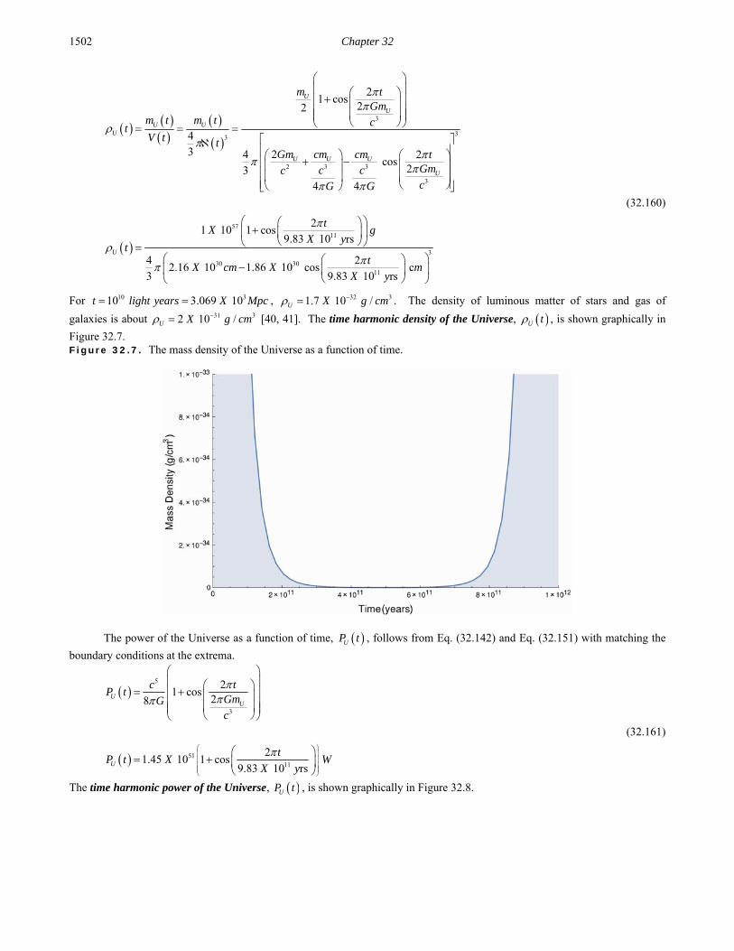
Chapter 32 1502
3
33
3 32
3
57 11
30
21 cos
22
43 24 2
cos23
4 4
21 10 1 cos
9.83 10 rs
42.16 10 1.86
3
U
U
U UU
U U U
U
U
m tGm
m t m t ctV t t
Gm cm cm tGmc cccG G
tX g
X yt
X cm X
3
30 11
2 10 cos c
9.83 10 rst
mX y
(32.160)
For 10 310 3.069 10t light years X Mpc , 32 31.7 10 /U X g cm . The density of luminous matter of stars and gas of
galaxies is about 31 32 10 /U X g cm [40, 41]. The time harmonic density of the Universe, U t , is shown graphically in
Figure 32.7. Figure 32.7. The mass density of the Universe as a function of time.
The power of the Universe as a function of time, UP t , follows from Eq. (32.142) and Eq. (32.151) with matching the
boundary conditions at the extrema.
5
3
51
11
21 cos
28
21.45 10 1 cos
9.83 10 rs
UU
U
c tP t
GmGc
tP t X W
X y
(32.161)
The time harmonic power of the Universe, UP t , is shown graphically in Figure 32.8.

Gravity 1503
Figure 32.8. The power of the Universe as a function of time.
The temperature of the Universe as a function of time can be derived from the Stefan-Boltzmann law. The Stefan-Boltzmann law (Eq. (32.143)) equates the power radiated by an object per unit area, R, to the emissivity, e, times the Stefan-Boltzmann constant, , times the fourth power of the temperature, 4T . The area of the Universe as a function of time, UA t ,
is approximately given by substitution of Eq. (32.153) into Eq. (32.144). (The Universe is a four-dimensional hyperspace of constant positive curvature at each r-sphere. In the case that the radius of the Universe is equal to the gravitational radius gr , the
area is given by Eq. (32.144); otherwise, the area of the sphere corresponding to the radius of the Universe is less than that given by Eq. (32.144). The proper area is given by solving Eq. (32.38) for the coordinate radius as a function of the proper radius followed by the substitution of the coordinate radius into Eq. (32.144)).
2
2 3 32
3
2
28 28 2
19
2 24 4 cos
2
4 4
24 2.16 10 1.86 10 cos
3.10 10 sec
U U UU
U
U
Gm cm cm tA t
Gmc cccG G
tA t X X m
X
(32.162)
The power radiated by the Universe per unit area as a function of time, UR t , is given by the ratio of Eq. (32.161) and Eq.
(32.162):
5
3
2
3 32
3
51 19
28 2
21 cos
28
2 24 cos
2
4 4
21.45 10 1 cos
3.10 10 sec
4 2.16 10 1.86 10
U
UU
U
U U U
U
U
c tGmG
P t cR tA t
Gm cm cm tGmc cccG G
tX W
XR t
X X
2
8 2 19
2cos
3.10 10 sect
mX
(32.163)

Chapter 32 1504
The temperature of the Universe as a function of time, UT t , follows from the Stefan-Boltzmann law (Eq. (32.143))
and Eq. (32.163).
1
4
5
31
42
3 32
3
5119
21 cos
28
2 24 cos
2
4 4
21.45 10 1 cos
3.10 10 sec
U
UU
U U U
U
U
c tGmGc
R tT t
eGm cm cm t
Gmc cccG G
e
tX
X
T t
1
4
2
28 28 2 19
8 2 4
24 2.16 10 1.86 10 cos
3.10 10 sec
5.67 10
W
tX X m
X
X Wm K
(32.164)
where the emissivity, e , for a blackbody is one, and 8 2 4 5.67 10X Wm K .
The Universe is a four-dimensional hyperspace of constant positive curvature at each r-sphere. The coordinates are spherical, and the space can be described as a series of spheres each of constant radius r whose centers coincide at the origin. The existence of the mass Um causes the area of the spheres to be less than 24 r and causes the clock of each r-sphere to run so
that it is no longer observed from other r-spheres to be at the same rate. The Schwarzschild metric given by Eq. (32.38) is the general form of the metric which allows for these effects. Fang and Ruffini [8] show that the time effect is equivalent to a gravitational redshift of a photon. The shifted wavelength due to the gravitational field of a mass Um is:
21 UGm
rc
(32.165)
Wien’s displacement law gives the relationship between temperature and wavelength [34].
3max 2.898 10 T X m K (32.166)
Thus, the temperature of the Universe as a function of time, UT t , is:

Gravity 1505
11 44
2
2 2
3
2 3 32
3
1 14
1 1
21 cos
22
1
2 2cos
2
4 4
UU
UU U
U
U
U
U U U
U
P tR t
T t tGm t Gm teec t c t
Gm tGm
cT t
Gm cm cm tc
Gmc cccG G
1
15 4
3
2
3 32
3
21 cos
28
2 24 cos
2
4 4
U
U U U
U
X
c tGmGc
Gm cm cm tGmc cccG G
e
(32.167)
1
27 11
28 28 11
51 11
20.74 10 1 cos
9.83 10 rs1
22.16 10 1.86 10 cos
9.83 10 rs
21.45 10 1 cos
9.83 10 rs
4 2.1
U
tX m
X yT t X
tX X m
X y
tX W
X y
1
4
2
28 28 11
8 2 4
26 10 1.86 10 cos
9.83 10 rs
5.67 10
tX X m
X y
X Wm K
(32.168)
The temperature of the Universe as a function of time, UT t , during the expansion phase is shown graphically in Figure 32.9.

Chapter 32 1506
Figure 32.9. The temperature of the Universe as a function of time during the expansion phase.
BOX 32.3 SIMPLIFIED SET OF COSMOLOGICAL EQUATIONS [42]
3
4 2Umc
QG T
2 4 2
U UG
U
Gm m c cT cr
c Q
where 2 /U T is the angular frequency of the Universe:
2
2
2U U
g
Gm m c cTr
c Q
Period of the Universe:
3
22
2G U Ur Gm m
Tc c Q
0 2Um ccT
Q
0 1 2 1 2 2 1 22
UU g
m c cTr r cT
Q
0 20.8627
1 2Ur
41 2 2 cos 2 1 2 2 cos 2 1 2 2 cos
2U
gU
m ct cT t Qr t
T T Q m
2 4 4
2 sin 4 sin 2 4 sinU U
d cT Q t Qt c c t
dt T m T m

Gravity 1507
3
3 33
2 3
32
11 cos 2
24 4
1 2 2 cos 23 3 2
41 cos
3
41 2 2 cos
UU
U
U
U
U
U
tm
m t Tt
m c tQ T
Qt
mQ
m c Qt
m
22 32
max 0 32 3 3 30
36 36
4 4U U U
U U tU g
m m mQt
m c r r cT
25
24 1 41 cos 1 cos 1 cos 2
8 2 4U
UU U
m cc Q Q tt t Qc t
G m m T T
2 48 2 44
3 2
2
1; 1; 5.6704 10
601
UU
U
R t kT t e Wm K
m t e cGc t
2 2
2
1 4 41 cos 1 cos2 1
4 42 4 1 2 2 cos1 2 2 cos
UU UU
U
UU
Q Qm t tm mm tG G
c t c QGm Q ttmc m
2
2 2 2
3
22
41 1 cos2
4 44 1 2 2 cos2
41 cos
2 4
1 2 2 cos
UUU
U
U
U
U
U
QtQc mP t
R tt m c Q
tQ m
Qt
mQ
m Qt
m
3 2 3
444 2
430 1 cos
4 41 cos 1 2 2 cos1
14 4
1 2 2 cos
UUU
U U
U
Qc Q tmk m
T tQ Qt tm m
Qt
m
3 23 2 3
4 2 3 4
3030
8U
U
m cc Q
k m T k

Chapter 32 1508
541 10 1 cos 2U
tm t kg
T
3
3 85 344.22 10 1 0.863 cos 2
3UU
tV t t mm
T
353 3
1 cos 2
2.37 10
1 0.863 cos 2
UUU
U
U
tTm t g
tV t mt
T
5
511 cos 2 1.444 10 1 cos 28U
U U
c t tt W
G T T
2
4UA
2
2
57 24 5.86 10 1 0.863 cos 2UU
tA t m
T
72 2
1 cos 2
2.46 10
1 0.863 cos 2
UUU
U
U
tTP t W
R tA t mt
T
1
4
1
4
1
2
1 cos 2
1.444
1 0.863 cos 2
UUU
U
tTR t
T t Ke
tT
1
4
2
1
4
1
2
2
1
1
1.444 1 cos 21
1 cos 21 0.863 cos 2
1 3.44 10
1 0.863 cos 2
UU
U
U
UU
U
R tT t
m t eGc t
tT
Kt
tT
Tt
T
0 max
1 1.1892 4.6391.444 3.089
1 0.502 0.3701 1.502U t UT t T K K K

Gravity 1509
COMPOSITION OF THE UNIVERSE In the case that lower-energy hydrogen, hydrinos, comprises the dark matter, all matter is ordinary (baryonic) matter, and the mass of the Universe is sufficient for it to be closed [30, 31]. Whereas, the standard theory of big bang nucleosynthesis explains the observed abundance of light elements (H, He, and Li) only if the present density of ordinary (baryonic) matter is less than 10 % of the critical value [43, 44]. Recently, the missing mass has been showed to be baryonic rather than strange matter [45]. According to classical physics (CP), the abundance of the lighter elements, H, He, and Li can be explained by neutron, proton, and electron production during the contraction phase and stellar nucleosynthesis during the contraction as well as the expansion phase of the expansion-contraction cycle. In the latter case, stellar and galaxy evolution occurred during the contraction phase as revealed by high-redshift radio galaxies and galaxies associated with extremely distant, luminous quasars that date back to the beginning of the expansion [46, 47]. The presence of metal lines in quasars demand a previous generation of stars (two generations for nitrogen) that is consistent with the stellar nucleosynthesis origin of the light elements [46].
The abundance of light elements for any r-sphere may be calculated using the power of the Universe as a function of time (Eq. (32.161)) and the stellar nucleosynthesis rates. During the contraction phase of the oscillatory cycle, the electron neutrino causes neutron production from a photon. Planck’s equation and special and general relativity define the mass of the neutron in terms of the spacetime metric as given in the Quarks section. The Planck equation energy, which is equal to the mass energy, applies for the proper time of the neutron given by general relativity (Eq. (32.38)) that is created with the transition of a photon to a neutron.
As discussed previously in the Quantum Gravity of Fundamental Particles section, ordinarily, a photon gives rise to a particle and an antiparticle. The event must be spacelike or annihilation would occur. The event must also conserve energy, momentum, charge, and satisfy the condition that the speed of light is a constant maximum. Eqs. (32.14-32.17) give the relationship whereby matter causes relativistic corrections to spacetime that determines the curvature of spacetime and is the origin of gravity. To satisfy the boundary conditions, particle production from a single photon requires the production of an antimatter particle as well as a particle. The transition state from a photon to a particle and antiparticle comprises two concentric atomic orbitals called transition state atomic orbitals. The gravitational effect of a spherical shell on an object outside of the radius of the shell is equivalent to that of a point of equal mass at the origin. Thus, the proper time of the concentric atomic orbital with radius *r (the radius is infinitesimally greater than that of the inner transition state atomic orbital with radius *r ) is given by the Schwarzschild metric, Eq. (32.38). The proper time applies to each point on the atomic orbital. Therefore, consider a general point in the xy-plane having Cr ; 0dr ; 0d ; 2sin 1 . Substitution of these parameters into Eq. (32.38)
gives:
12 2
02 * 2
21
Gm vd dt
c r c
(32.169)
with 2 2v c , Eq. (32.169) becomes
2 * 2
2 2
c
GM GMti ti
c r c
(32.170)
The coordinate time is imaginary because particle/antiparticle production is spacelike. The left-hand side of Eq. (32.170) represents the proper time of the particle/antiparticle as the photon atomic orbital becomes matter. The right-hand side of Eq. (32.170) represents the correction to the laboratory coordinate metric for time corresponding to the curvature of spacetime by the particle production event.
In contrast to the familiar particle production event involving production of particles in matter-antimatter pairs, it is possible to form a particle without production of the corresponding antimatter partner. During the contraction phase, electron neutrinos cause neutron production from photons. In this case, the event must also be spacelike or annihilation would occur. Similarly, the event must also conserve energy, momentum, charge, and satisfy the condition that the speed of light is a constant maximum. Eqs. (32.14-32.17) also apply. They give the relationship whereby matter causes relativistic corrections to spacetime that determines the curvature of spacetime and is the origin of gravity.
The electron neutrino is a special type of photon as given in the Neutrino section. It travels at the speed of light for all observers and is not a particle with non-zero rest mass. In addition, neutrinos have spin which must be conserved. To satisfy the boundary conditions, particle production from an electron neutrino and a photon requires the production of a single neutral particle, a neutron. In this case, the transition state only comprises a single transition state atomic orbital. The left-hand side of Eq. (32.170) represents the proper time of the neutron as the photon atomic orbital becomes matter. The right-hand side of Eq. (32.170) represents the correction to the laboratory coordinate metric for time corresponding to the relativistic correction of spacetime by the particle production. Thus, during the contraction phase of the oscillatory cycle, the electron neutrino causes neutron production from a photon, and the production of protons and electrons occurs by neutron beta decay.
Typically, antimatter and matter are created in the laboratory in equal amounts; yet, celestial antimatter is not observed. The reason is that electron neutrinos of only one type (electron neutrinos versus electron antineutrinos) exist at the initiation of spacetime contraction. Thus, spin conservation requires that antineutron production does not occur as a separate symmetrical reaction, and particle production from a neutrino and a photon prohibits production of the antimatter twin. From Eq. (38.6), the neutron mass is

Chapter 32 1510
1 1
2 427
2
1 2 2 (3)(3)(2 ) 1.674 10
1 sec 2ddu calculated
h chm X kg
c G
(32.171)
The neutron production reaction and the nuclear reaction for the beta decay of a neutron are:
1
1 1 0.7835
e
e
n
n H MeV
(32.172)
where e is the electron neutrino and e is the electron antineutrino. Eq. (32.172) predicts an electron neutrino background
which could account for the atmospheric neutrino anomaly [48]. From Eq. (32.172), the number of electrons exactly balances the number of protons. Thus, the Universe is electrically neutral.
Thus, the Universe is oscillatory in matter, energy, and spacetime without the existence of antimatter due to conservation of spin of the electron neutrino and the relationship of particle production to spacetime contraction. During the expansion phase, the arrow of time runs forward to lower mass and higher entropy states; whereas, during collapse, the arrow of time runs backwards relative to the case of the Universe in a state of expansion. Recent particle physics experiments demonstrate that the decay of kaons and antikaons follows a law that is not symmetric with respect to time reversal [39]. The data reveals that there is a microscopic arrow of time, in addition to the thermodynamic and cosmological arrows.
The Universe evolves to higher mass and lower entropy states. Thus, biological organisms such as humans, which rely on the spontaneity of chemical reactions with respect to the forward arrow of time cannot exist in the contracting phase of the Universe. And, compared to the period of the Universe, the origins of life occurred at a time very close to the beginning of the expansion of the Universe when the direction of the spontaneity of reactions changed to the direction of increasing entropy and the rate of the increase in entropy of the Universe was a maximum.
The origin of the microwave background radiation (CMBR) as the power from the Universe rather than from a Big Bang creation event is demonstrated by the absence of the shadows in the CMBR required for the Big Bang model [36]. As shown in the Power Spectrum of the Cosmic Microwave Background section, when the Universe reaches the maximum radius of the time harmonic variation in the radius of the Universe, (Eq. (32.150)), it is entirely radiation filled. Since the photon has no gravitational mass, the radiation is uniform. As energy converts into matter the power of the Universe may be considered negative for the first quarter cycle starting from the point of maximum expansion as given by Eq. (32.195), and spacetime contracts according to Eq. (32.140). The gravitational field from particle production travels as a light wave front. As the Universe contracts to a minimum radius, the gravitational radius given by Eq. (32.147), constructive interference of the gravitational fields occurs. The resulting slight variations in the density of matter are observed from our present r-sphere. As shown in the Power Spectrum of the Cosmic Microwave Background section, the cosmic microwave background radiation is an average temperature of 2.725 K, with deviations of 30 or so K in different parts of the sky representing these slight variations in the density of matter. By this mechanism, the production of particles over time from a photon-filled Universe gave rise to centers that eventually aggregated by gravitational attraction into a hierarchy of more massive structures to eventually form the large-scale structure of the cosmos.
Galaxies formed during the collapsing stage of the evolution of the Universe wherein the mass perturbations occurred due to gravity wave interference as demonstrated by the DASI and WMAP data as shown in the Power Spectrum of the Cosmic Microwave Background section. These perturbations resulted in collapsing gas clouds that formed quasars. Then each of these quasars erupted into a supernova and formed a blackhole. The expelled gas eventually formed galaxies. The observation of a blackhole in the center of each galaxy is consistent with the origin of galaxies from a quasar supernova [49, 50]. Furthermore, since angular momentum must be conserved in the rotation of the founding quasar and the resulting blackhole and galactic rotating stars, a linear relationship of the plot of the velocity of the outer stars of a given galaxy to the blackhole mass is expected. This ratio called sigma is indeed observed to be linear [49, 50].
The Universe is oscillatory with a finite minimum radius, the gravitational radius. Thus, stellar and celestial structures evolve on a time scale that is greater than the observed time of expansion. Stars exist which are older than the elapsed time of the present expansion as stellar evolution occurred during the contraction phase [51, 52]. Galaxy evolution also occurred during the contraction phase as revealed by high-redshift radio galaxies and galaxies associated with extremely distant, luminous quasars that date back to the beginning of the expansion [46, 47]. The Gemini Deep Deep Survey confirmed the predicted existence of old galaxies at the beginning of the expansion at 10 billion light years and further directly disprove the Big Bang theory of cosmology [53-55]. These results were confirmed by a spectroscopic redshift survey that probed the most massive and quiescent galaxies back at 10 billion light years [56, 57]. It was found that a significant fraction of the massive old galaxies observed over all of time since the expansion were in place in the early Universe. This is also shown by the Hubble Ultra Deep Field (HUDF) given in Figure 32.10. Recently, a definitive validation of the classical predictions was provided by the Keck survey for gravitationally lensed Ly emitters that found galaxies back at over 13 billion light years [58]. The absence of red dwarf stars that contain no metals is another indication of the ancient nature of the universe that is much older than the 10 billion years of expansion. Further confirmation of the older age of the universe is the existence of the brightest quasar in the early universe powered by the most massive black hole yet known [59] and that dust, a signature of an old galaxy, has been observed in a young universe [60].

Gravity 1511
Figure 32.10 . The Hubble Ultra Deep Field (HUDF) shows mature galaxies at the time of the beginning of the expansion of the Universe. The “Big Bang” is NOT observed. This image is a composite of two separate images taken by the Hubble’s Advanced Camera for Surveys (ACS) and the Near Infrared Camera and Multiobject Spectrometer (NICMOS), the result of over eleven and a half days of exposure. It contains an estimated ten thousand galaxies. Released on 9 March 2004. Courtesy of NASA, ESA, S. Beck with STScI and the HUDF Team.
In addition to fusion reactions in stars, hydrino transitions to lower energy hydrino states is a source of power contribution to the CMBR as well as a source of spacetime expansion as matter is converted into energy. As given in the Disproportionation of Energy States section, classical physical laws predict that atomic hydrogen may undergo a catalytic reaction with certain species, including itself, that can accept energy in integer multiples of the potential energy of atomic hydrogen, m · 27.2 eV, wherein m is an integer. The predicted reaction involves a resonant, nonradiative energy transfer from otherwise stable atomic hydrogen to the catalyst capable of accepting the energy. The product is H(1/p), fractional Rydberg states of atomic hydrogen called “hydrino atoms,” wherein n = 1/2, 1/3, 1/4,…, 1/p (p≤137 is an integer) replaces the well-known parameter n = integer in the Rydberg equation for hydrogen excited states. Each hydrino state also comprises an electron, a proton, and a photon, but the field contribution from the photon increases the binding energy rather than decreasing it corresponding to energy desorption rather than absorption. Since the potential energy of atomic hydrogen is 27.2 eV, m H atoms serve as a catalyst of 27.2 m eV for another ( 1m )th H atom (See BlackLight Process section). For example, a H atom can act as a catalyst for another H by accepting 27.2 eV from it via through-space energy transfer such as by magnetic or induced electric dipole-dipole coupling to form an intermediate that decays with the emission of continuum bands with short
wavelength cutoffs and energies of 22
91.213.6
m eV nm
m
. The continuum radiation band at 10.1 nm and going to longer
wavelengths for theoretically predicted transitions of H to lower-energy, so called “hydrino” state H(1/4), was observed only arising from pulsed pinch gas discharges comprising some hydrogen and oxygen as an oxide, first at BlackLight Power, Inc. (BLP) and reproduced at the Harvard Center for Astrophysics (CfA) [61-66]. HOH was shown to be the catalyst in these pinch plasma continua as well as in the 10-30 nm EUV continuum observed from plasma having essentially no field. The latter plasma was formed by igniting a solid fuel source of H and HOH catalyst by passing an ultra-low voltage, high current through the fuel to produce an explosive plasma [61]. Moreover, m H catalyst (Eqs. (5.48-5.61)) was identified to be active in astronomical sources such as the Sun, stars, and interstellar medium wherein the characteristics of hydrino product match those of the dark matter of the Universe [61]. Hydrogen continua from transitions to form hydrinos matches the emission from white dwarfs, provides a possible mechanism of linking the temperature and density conditions of the different discrete layers of the coronal/chromospheric sources, and provides a source of the diffuse ubiquitous EUV cosmic background with the 10.1 nm continuum matching the observed intense 11.0-16.0 nm band in addition to resolving other cosmological mysteries [61,65,67,68]. Given the seeding by the anisotropic gravitational forces in a contracting Universe, expansion of the Universe depends on the rate of energy release, which varies throughout the Universe; thus, clusters of galaxies, huge voids, and other large features which are observed [69-73] are caused by the interaction between the rate of energy release with concomitant spacetime expansion and gravitational attraction. Hydrogen-type atoms and molecules comprise most of the matter of the Universe. The distinction between hydrogen and hydrinos with respect to the interaction with electromagnetic radiation and release of energy by transitioning to lower energy states (See Disproportionation of Energy States section) also has an influence

Chapter 32 1512
on the formation of large voids and walls of matter. Lower-energy atomic hydrogen atoms, hydrinos, each have the same mass and a similar interaction as the neutron. According to Steinhardt and Spergel of Princeton University [74], these are the properties of dark matter that are necessary in order for the theory of the structure of galaxies to work out on all scales. The observation that galaxy clusters arrange themselves as predicted for cold dark matter except that the cores are less dense than expected is explained. Hydrinos further account for the observation that small halos of dark matter are evaporated when they approach larger ones and that dark matter is easily influenced by black holes, explaining how they grew so large.
Laboratory EUV continuum results [61] offer resolution to many otherwise inexplicable celestial observations with (a) the energy and radiation from the hydrino transitions being the source of extraordinary temperatures and power regarding the solar corona problem, the cause of sunspots and other solar activity, and why the Sun emits X-rays [65], (b) the hydrino-transition radiation being the radiation source heating the WHIM and behind the observation that diffuse H emission is ubiquitous throughout the Galaxy requiring widespread sources of flux shortward of 912 Å , and (c) the identity of dark matter being hydrinos.
Stars also comprise plasmas of hydrogen with surfaces comprised of essentially dense atomic hydrogen permissive of multi-body H interactions to propagate transition of H to H(1/(m +1)) wherein m H serves as the catalyst. Such transitions are predicted to emit EUV continuum radiation according to Eqs. (5.48-5.61). The emission from white dwarfs arising from an extremely high concentration of hydrogen is modeled as an optically thick blackbody of ~ 50,000 K gas comprising predominantly hydrogen and helium. A modeled composite spectrum of the full spectral range from 10 nm to >91.2 nm with an abundance He/H=10-5 from Barstow and Holberg [67] is shown in Figure 10 of Ref. [61]. Albeit, while white dwarf spectra can be curve fitted using stratification and adjustable He and H column densities and ionization fractions to remove some inconsistencies between optical and EUV spectra [75] and independent measurements of the latter, matching the spectrum at the short-wavelengths is problematic. Alternatively, combining the laboratory-observed emission continuum bands gives a spectrum with continua having edges at 10.1 nm, 22.8, nm, and 91.2 nm, a match to the white dwarf spectrum [61]. However, the proposed nature of the plasmas and the mechanisms are very different. The emission in our studies is assigned to hydrino transitions in cold-gas, optically-thin plasmas absent any helium. White-dwarf and celestial models may need revision and benefit from our discovery of high-energy H continua emission.
For example, there is no existing physical model that can couple the temperature and density conditions in different discrete regions of the outer atmosphere (chromosphere, transition region, and corona) of coronal/chromospheric sources [75]. Typically, the corona is modeled to be three orders of magnitude hotter than the surface that is the source of coronal heating seemingly in defiance of the second law of thermodynamics. Reconciliation is offered by the mechanism of line absorption and re-emission of the 2 13.6 m eV (Eq. (5.57)) continuum radiation. The 91.2 nm continuum to longer wavelengths is expected to be prominent (less attenuated than the 10.1 nm and 22.8 nm bands) and is observed in the solar extreme ultraviolet spectrum as shown in Figure 11 of Ref. [61] and Ref. [76] despite attenuation by the coronal gas. High-energy-photon excitation is more plausible than a thermal mechanism with T~106 given the 4000 K surface temperature and the observation of the CO absorption band at 4.7 m in the solar atmosphere wherein CO cannot exist above 4000 K [77]. Considering the 10.1 nm band as a source, the upper limit of coronal temperature based on excitation of about 106 K is an energy match. In addition to the temperature, another extraordinary observation is that although the total average energy output of the outer layers of the Sun is 0.01 % of the photospheric radiation, local transient events can produce an energy flux that exceeds the photospheric flux [78]. The energy source of the latter may be magnetic in nature, but identity of the highly ionizing coronal source is not established. Nor, has the total energy balance of the Sun been reconciled. The possibility of a revolutionary discovery of a new source of energy in the Sun based on a prior undiscovered process is an open question [79]. That m H catalyzed hydrino transitions occur in stars and the Sun [80] as evident by corresponding continua in its spectrum resolves the solar corona problem, the cause of sunspots and other solar activity, and why the Sun emits X-rays [65].
The laboratory EUV continuum results [61] have further implications for the resolution of the identity of dark matter and the identity of the radiation source behind the observation that diffuse H emission is ubiquitous throughout the Galaxy and widespread sources of flux shortward of 912 Å are required [81]. The identity of dark matter has been a cosmological mystery. It is anticipated that the emission spectrum of the extreme ultraviolet background of interstellar matter possesses the spectral signature of dark matter. Labov and Bowyer designed a grazing incidence spectrometer to measure and record the diffuse extreme ultraviolet background [81]. The instrument was carried aboard a sounding rocket, and data were obtained between 80 Å and 650 Å (data points approximately every 1.5 Å ). Several lines including an intense 635 Å emission associated with dark matter were observed [81] which has considerable astrophysical importance as indicated by the authors:
"Regardless of the origin, the 635 Å emission observed could be a major source of ionization. Reynolds (1983, 1984,
1985) has shown that diffuse H emission is ubiquitous throughout the Galaxy, and widespread sources of flux shortward of 912 Å are required. Pulsar dispersion measures (Reynolds 1989) indicate a high scale height for the associated ionized material. Since the path length for radiation shortward of 912 Å is low, this implies that the ionizing source must also have a large scale height and be widespread. Transient heating appears unlikely, and the steady state ionization rate is more than can be provided by cosmic rays, the soft X-ray background, B stars, or hot white dwarfs (Reynolds 1986; Brushweiler & Cheng 1988). Sciama (1990) and Salucci & Sciama (1990) have argued that a variety of observations can be explained by the presence of dark matter in the galaxy which decays with the emission of radiation below 912 Å .

Gravity 1513
The flux of 635 Å radiation required to produce hydrogen ionization is given by F H / 4.3 X 10413 photons cm2s1 , where 13 is the ionizing rate in units of 1013s1 per H atom. Reynolds (1986) estimates that in the immediate vicinity of the Sun, a steady state ionizing rate of 13 between 0.4 and 3.0 is required.
To produce this range of ionization, the 635 Å intensity we observe would have to be distributed over 7% - 54% of the sky." The 63.5 0.47 nm line [81] matches a hydrino transition predicted for H undergoing catalysis with H (m=1) as the catalyst giving rise to a concerted energy exchange of the total energy of 40.8 eV with the excitation of the He 1s2 to 1s12p1 transition. The predicted 63.3 nm emission associated with dark matter was observed with the addition of hydrogen to helium microwave plasma as shown previously [65,82]. An alternative assignment suggested by Labov and Bowyer [81] is the 63.0 nm line of O V requiring a large-scale non-thermal source of ionization. Continuum radiation from transitions to low-level hydrino states can provide this radiation. Indeed, the observation of the 63.3 nm line is also associated with the presence of an interstellar X-ray background.
The first soft X-ray background was detected and reported [83] about 25 years ago. Quite naturally, it was assumed that these soft X-ray emissions were from ionized atoms within hot gases. Labov and Bowyer also interpreted the data as emissions from hot gases. However, the authors left the door open for some other interpretation with the following statement from their introduction:
"It is now generally believed that this diffuse soft X-ray background is produced by a high-temperature component of the interstellar medium. However, evidence of the thermal nature of this emission is indirect in that it is based not on observations of line emission, but on indirect evidence that no plausible non-thermal mechanism has been suggested which does not conflict with some component of the observational evidence."
The authors also state "if this interpretation is correct, gas at several temperatures is present." Specifically, emissions
were attributed to gases in three ranges: 5.5 < log T < 5.7; log T = 6; 6.6 < log T < 6.8. Observations in the ultraviolet with HST and FUSE [84] and also XMM-Newton [85] confirm these extraordinary temperatures of diffuse intergalactic medium (IGM) and reveal that a large component of the baryonic matter of the Universe is in the form of WHIM (warm-hot ionized media) [84,85]. The mysteries of the identity of dark matter, the observed dark interstellar medium spectrum, the source of the diffuse X-ray background, and the source of ionization of the IGM [84,85] are resolved by the formation of hydrinos that emit EUV and X-ray continua depending on the state transition and conditions; the continua create highly ionized ions that emit ion radiation of non-thermal origin; the hydrino transition H to H(1/2) results in a 63.3 nm line [65,82], and He+ acting as a catalyst of 54.4 eV ( 2 27.2 eV ) pumps the intensity of helium ion lines such as the 30.4 nm line [63,65].
As shown in the Disproportionation of Energy States section, the products of the catalysis reactions (e.g. Eqs. (5.48-5.51)) have binding energies of 27.2 m eV , such that they may further serve as catalysts. Thus, further catalytic transitions may
occur: 1 1 1 1
, ,3 4 4 5
n and so on. Thus, lower-energy hydrogen atoms, hydrinos, can act as catalysts by resonantly and
nonradiatively accepting energy of 27.2 m eV from another H or hydrino atom (Eq. (5.24)). Such disproportionation reactions of hydrinos are predicted to give rise to features in the X-ray region. As shown by Eqs. (5.40-5.43) the reaction product of HOH
catalyst is Ha
H
4
. A likely transition reaction in hydrogen clouds containing H2O gas is the transition of a H atom to
17Ha
H
wherein Ha
H
4
serves as a catalyst to give a broad peak having a short wavelength cutoff at E 3481.6 eV ; 0.35625 nm . A
broad X-ray peak with a 3.48 keV cutoff was recently observed in the Perseus Cluster by NASA’s Chandra X-ray Observatory and by the XMM-Newton [86,87] that has no match to any known atomic transition. The 3.48 keV feature assigned to dark
matter of unknown identity by BulBul et al. [86] matches the 4 1 17H H Ha a a
H H H
transition and further confirms
hydrinos as the identity of dark matter. Evidence for EUV emission from hydrino transitions also comes from the interstellar medium (ISM) since it provides a
source of the diffuse ubiquitous EUV cosmic background. Specifically, the 10.1 nm continuum matches the observed intense 11.0-16.0 nm band [67,68]. Furthermore, it provides a mechanism for the high ionization of helium of the ISM and the excess EUV radiation from galaxy clusters that cannot be explained thermally [86]. Moreover, recent data reveals that X-rays from distant active galactic nuclei sources are absorbed selectively by oxygen ions in the vicinity of the galaxy [87]. The temperature of the absorbing halo is between 1 million and 2.5 million Kelvin, or a few hundred times hotter than the surface of the Sun. The corresponding energy range is 86 eV to 215 eV which is in the realm of the energy released for the transition of H to H(1/4). Additional astrophysical evidence such as the observation that a large component of the baryonic matter of the Universe is in the form of WHIM (warm-hot ionized media) in the absence of a conventional source and the match of hydrinos to the identity of dark matter was presented previously [65]. The latter case is further supported by observations of signature electron-positron annihilation energy.
Dark matter comprises a majority of the mass of the Universe as well as intra-galactic mass [90,91]. It would be

Chapter 32 1514
anticipated to concentrate at the center of the Milky Way galaxy due to the high gravity from the presence of a super massive blackhole at the center that emits gamma rays as matter falls into it. Since hydrinos are each a state of hydrogen having a proton nucleus, high-energy gamma rays impinging on dark matter will result in pair production. The corresponding observed characteristic signature being the emission of the 511 keV annihilation energy of pair production identifies dark matter as hydrino [92-94]. Another hydrino decay pathway for this radiation is given by Eq. (32.173). The interstellar medium [95-97], gamma-ray bursts [97,98], and solar flares [77,97,99] also emit 511 keV line radiation. The dominant source of positrons in gamma-ray bursts is likely pair production by photon on photons or on strong magnetic fields [97]. The solar-flare emission is likely due to production of radioactive positron emitters in accelerated charge interactions [97]; whereas, the diffuse 511 keV radiation by interstellar medium is consistent with the role of hydrino as dark matter in pair production from incident cosmic radiation [95-97].
The characteristic spectral signatures and properties of hydrino match those attributed to the dark matter of the Universe. The Universe is predominantly comprised of hydrogen and a small amount of helium. These elements exist in interstellar regions of space, and they are expected to comprise the majority of interstellar matter. However, the observed constant angular velocity of many galaxies as the distance from the luminous galactic center increases can only be accounted for by the existence of nonluminous weakly interacting matter, dark matter. It was previously accepted that dark matter exists at the cold fringes of galaxies and in cold interstellar space. This has since been disproved by the observation of Bournaud et al. [90,91] that demonstrated that galaxies are mostly comprised of dark matter, and the data persistently supports that dark matter probably accounts for the majority of the universal mass.
The best evidence yet for the existence of dark matter is its direct observation as a source of massive gravitational mass evidenced by gravitational lensing of background galaxies that does not emit or absorb light as shown in Figure 32.11 [100]. There has been the announcement of some unexpected astrophysical results that support the existence of hydrinos. In 1995, Mills published the GUTCP prediction [101] that the expansion of the Universe was accelerating from the same equations that correctly predicted the mass of the top quark before it was measured. To the astonishment of cosmologists, this was confirmed by 2000. Mills made another prediction about the nature of dark matter based on GUTCP that may be close to being confirmed. Bournaud et al. [90,91] suggest that dark matter is hydrogen in dense molecular form that somehow behaves differently in terms of being unobservable except by its gravitational effects. Theoretical models predict that dwarfs formed from collisional debris of massive galaxies should be free of nonbaryonic dark matter. So, their gravity should tally with the stars and gas within them. By analyzing the observed gas kinematics of such recycled galaxies, Bournaud et al. [90,91] have measured the gravitational masses of a series of dwarf galaxies lying in a ring around a massive galaxy that has recently experienced a collision. Contrary to the predictions of Cold-Dark-Matter (CDM) theories, their results demonstrate that they contain a massive dark component amounting to about twice the visible matter. This baryonic dark matter is argued to be cold molecular hydrogen, but it is distinguished from ordinary molecular hydrogen in that it is not traced at all by traditional methods, such as emission of CO lines. These results match the predictions of the dark matter being molecular hydrino. Figure 32.11 . Dark matter ring in galaxy cluster. This Hubble Space Telescope composite image shows a ghostly “ring” of dark matter in the galaxy cluster Cl 0024+17. The ring is one of the strongest pieces of evidence to date for the existence of dark matter, a prior unknown substance that pervades the Universe. Courtesy of NASA, M.J. Jee and H. Ford (Johns Hopkins University).

Gravity 1515
Additionally, astronomers Jee at al. [102] using data from NASA’s Hubble Telescope have mapped the distribution of dark matter, galaxies, and hot gas in the core of the merging galaxy cluster Abell 520 formed from a violent collision of massive galaxy clusters and have determined that the dark matter had collected in a dark core containing far fewer galaxies than would be expected if dark matter was collsionless with dark matter and galaxies anchored together. The collisional debris left behind by the galaxies departing the impact zone behaved as hydrogen did, another indication that the identity of dark matter is molecular hydrino. Moreover, detection of alternative hypothesized identities for dark matter such as super-symmetry particles such as neutalinos has failed at the Large Hadron Collider; nor, has a single event been observed for weakly interacting massive particles or wimps at the Large Underground Xenon (LUX) experiment [103]. The HADES search for dark matter eliminated the leading candidate, “Dark Photon” or U Boson, as a possibility. This failure also undermines the Standard Model of particle physics [104].
During the expansion phase, protons and electrons of hydrinos which comprises the dark matter annihilate to photons and electron neutrinos as given in the New “Ground” State section. To conserve spin (angular momentum) the reaction is:
1 He e
aH
p
(32.173)
where e is the electron neutrino. (A similar reaction to that of Eq. (32.173) is the reaction of a muon neutrino rather than an
electron antineutrino with a hydrino to give a gamma photon and a muon antineutrino.) Disproportionation reactions to the lowest-energy states of hydrogen followed by electron capture with gamma ray emission may be a source of nonthermal -ray
bursts from interstellar regions [105]. A branch of the decay path may also be similar to that of the 0 meson. Gamma and pair-production decay would result in characteristic 511 keV annihilation energy emission. This emission has been recently been identified with dark matter [106,107].
Furthermore, a very plausible source of nonthermal -ray bursts from interstellar regions [105] may be due to conversion of matter to photons of the Planck mass-energy, which may also give rise to cosmic rays. When the gravitational potential energy density of a massive body such as a blackhole equals that of a particle having the Planck mass as given by Eqs. (32.22-32.32), the matter may transition to photons of the Planck mass given by Eq. (32.31). In the case of the Planck mass, the gravitational potential energy (Eq, (32.30)) is equal to the Planck, electric, and magnetic energies which equal 2mc (Eq. (32.32)), and the coordinate time is equal to the proper time (Eqs. (32.33-32.34) and Eq. (32.43)). However, the particle corresponding to the Planck mass may not form since its gravitational velocity (Eq. (32.33)) is the speed of light. (The limiting speed of light eliminates the singularity problem of Einstein’s equation that arises as the radius of a blackhole equals the Schwarzschild radius. General relativity with the singularity eliminated resolves the paradox of the infinite propagation velocity required for the gravitational force in order to explain why the angular momentum of objects orbiting a gravitating body does not increase due to the finite propagation delay of the gravitational force according to special relativity [108]). Thus, it remains a photon. Even light from a blackhole will escape when the decay rate of the trapped matter with the concomitant spacetime expansion is greater than the effects of gravity that oppose this expansion. The annihilation of a blackhole may be the source of g-ray bursts. Gamma-ray bursts are the most energetic phenomenon known that can release an explosion of gamma rays packing 100 times more energy than a supernova explosion [109]. Cosmic rays are the most energetic particles known, and their origin is also a mystery [110]. In 1966, Cornell University’s Kenneth Greisen predicted that interaction with the ubiquitous photons of the cosmic microwave background would result in a smooth power-law cosmic-ray energy spectrum being sharply cutoff close to 195 10 X eV . However, in 1998, Schwarzschild reported [111] that the Akeno Giant Air Shower Array (AGASA) in Japan has collected data that show the cosmic-ray energy spectrum is extending beyond the Greisen-Zatsepin-Kuzmin (GZK) cutoff. According to the GZK cutoff, the cosmic spectrum cannot extend beyond 195 10 X eV , but AGASA, the world’s largest air shower array, has shown that the spectrum is extending beyond without any clear sign of cutoff. Similarly, the Utah Fly’s Eye had detected cosmic rays with energy up to 203 10 X eV [112,113]. Photons, each of the Planck mass, may be the source of these inexplicably energetic cosmic rays corresponding to tremendous power and concomitant spacetime expansion. The Planck mass conversion of matter into energy may also be the unprecedented X-ray power of the ultraluminous pulsar: NuSTAR [114]. The gamma ray burst energy may undergo energy down conversion by interaction with matter due to higher energy absorption and re-emission of lower energy gamma rays.
In addition to these novel mechanisms for the conversion of matter into energy, a light filled from a matter filled universe may be the result from a subtle change in the fundamental constants due to spacetime expansion to the maximum radius. There is evidence that with time evolution (spacetime expansion and contraction) the fine structure constant changes as an inherent property [115-118]. This would have a profound effect on stability and the inter-conversion rates of matter and energy. Matter filled universe may regard the maximum matter content, and light filled universe may regard the maximum light content wherein pure matter filled and pure light filled only regard one r-sphere at the extrema.
POWER SPECTRUM OF THE COSMOS The maximum energy release of the Universe given by Eq. (32.142) occurred at the beginning of the expansion phase, and the power spectrum is a function of the r-sphere of the observer. The power spectrum of the cosmos, as measured by the Las Campanas survey, generally follows the prediction of cold dark matter on the scales of 200 million to 600 million light-years. However, the power increases dramatically on scales of 600 million to 900 million light-years [50]. This discrepancy means that

Chapter 32 1516
the Universe is much more structured on those scales than current theories can explain. The Universe is oscillatory in matter/energy and spacetime with a finite minimum radius. The minimum radius of the Universe, 300 billion light years [32], is larger than that provided by the current expansion, approximately 10 billion light years [28]. The Universe is a four-dimensional hyperspace of constant positive curvature at each r-sphere. The coordinates are spherical, and the space can be described as a series of spheres each of constant radius r whose centers coincide at the origin. The existence of the mass Um causes the area
of the spheres to be less than 24 r and causes the clock of each r-sphere to run so that it is no longer observed from other r-spheres to be at the same rate. The Schwarzschild metric given by Eq. (32.38) is the general form of the metric that allows for these effects. Consider the present observable Universe that has undergone expansion for 10 billion years. The radius of the Universe as a function of time from the coordinate r-sphere is of the same form as Eq. (32.153). The average size of the Universe, Ur , is given as the sum of the gravitational radius, gr , and the observed radius, 10 billion light years.
10
11 10
11
10
3.12 10 10
3.22 10
U g
U
U
r r light years
r X light years light years
r X light years
(32.174)
The frequency of Eq. (32.153) is one half the amplitude of spacetime expansion from the conversion of the mass of Universe into energy according to Eq. (32.140). Thus, keeping the same relationships, the frequency of the current expansion function is the reciprocal of one half the current age. Substitution of the average size of the Universe, the frequency of expansion, and the amplitude of expansion, 10 billion light years, into Eq. (32.153) gives the radius of the Universe as a function of time for the coordinate r-sphere.
11 10
9
23.22 10 1 10 cos
5 10
tX light years X light years
X light years
(32.175)
The Schwarzschild metric gives the relationship between the proper time and the coordinate time (Eq. (32.38)). The infinitesimal temporal displacement, 2d , is:
2
2 2 2 2 2 2 22 2
2
2 11 sin
21
U
U
Gm drd dt r d r d
Gmc r cc r
(32.176)
In the case that 2 2 2 0dr d d , the relationship between the proper time and the coordinate time is:
2 22
21 UGm
d dtc r
(32.177)
2
21 UGm
tc r
(32.178)
1 grtr
(32.179)
The maximum power radiated by the Universe is given by Eq. (32.142) and occurs when the proper radius, the coordinate radius, and the gravitational radius gr are equal. For the present Universe, the coordinate radius is given by Eq. (32.174). The
gravitational radius is given by Eq. (32.147). The maximum of the power spectrum of a trigonometric function occurs at its frequency [119]. Thus, the coordinate maximum power according to Eq. (32.175) occurs at 95 10 X light years . The maximum
power corresponding to the proper time is given by the substitution of the coordinate radius, the gravitational radius gr , and the
coordinate power maximum into Eq. (32.179). The power maximum in the proper frame occurs at:
11 9
11
6
3.12 10 5 10 1
3.22 10
880 10
X light yearsX light years
X light years
X light years
(32.180)
The power maximum of the current observable Universe is predicted to occur on the scale of 6880 10 X light years . There is excellent agreement between the predicted value and the experimental value of between 600 million to 900 million light years [120].
THE DIFFERENTIAL EQUATION OF THE RADIUS OF THE UNIVERSE The differential equation of the radius of the Universe, , can be derived as a conservative simple harmonic oscillator having a restoring force, F , which is proportional to the radius. The proportionality constant, k , is given in terms of the potential energy, E , gained as the radius decreases from the maximum expansion to the minimum contraction.

Gravity 1517
2
Ek
(32.181)
The Universe oscillates between a minimum and maximum radius as matter is created into energy and then energy is converted to matter. At the minimum radius, the gravitational velocity, Gv , is given by Eq. (32.33) and the gravitational radius Gr , is given
by Eq. (32.22) wherein an electromagnetic wave of mass energy equivalent to the mass of the Universe travels in a circular orbit wherein the eccentricity is equal to zero (Eq. (35.21)), and the escape velocity from the Universe can never be reached. At this point in time, all of the energy of the Universe is in the form of matter, and the gravitational energy (Eq. (32.148)) is equal to
2Um c . Thus, the proportionality constant of the restoring force with respect to the radius is:
2 2
22
2
U U
G U
m c m cF k
r Gm
c
(32.182)
Considering the oscillation, the differential equation of the radius of the Universe, , follows from Eq. (32.182) as given by Fowles [121]:
2
2
2
2
2
0
0
UU
G
UU
U
m cm
r
m cm
Gm
c
(32.183)
The solution of Eq. (32.183) which gives the radius of the Universe as a function of time follows from Fowles [121]:
3 32
3
2cos
2
2 2cos
2
4 4
U Ug
G
U U U
U
cm cm tr
rQ Qc
Gm cm cm tGmc cccG G
(32.184)
The gravitation force causes the radius of Eq. (32.184) to be offset [121]. After Eq. (32.38), the force equations of general relativity give the offset radius, Ur . The minimum radius corresponds to the gravitational radius gr whereby the proper time is
equal to the coordinate time. The offset radius, Ur , is:
3
4
UU g
cmr r
cG
(32.185)
The expansion/contraction rate,
, is given by taking the derivative with respect to time of Eq. (32.184):
3
24 sin
2 U
tc
Gm
c
(32.186)
According to special relativity no signal may travel faster than c , the speed of light for any observer. The maximum expansion
rate for a 3-sphere is 4 c which is given in Eq. (32.186). The expansion/contraction acceleration,
, is given by taking the derivative with respect to time of Eq. (32.186).:
4
3
24 cos
2 UU
c tGmGmc
(32.187)
The Universe oscillates between the extremes of all matter and all energy. At the beginning of its expansion, the Universe is all matter with no electromagnetic radiation; thus, the Universe is not observable for earlier times. The observer’s light sphere determines the limits of observation thereafter. Furthermore, ancient stars and the large-scale structure of the cosmos comprising galactic superclusters and voids that could not have formed within the elapsed time of expansion are visible [50-57,69-73,122,123]. Recently, a uniform cosmic infrared background has been discovered which is consistent with the heating of dust with reradiation over a much longer period than the elapsed time of expansion [124]. The size of the Universe may be detected by observing the early curvature, the power spectrum, and the microwave background temperature. In the latter case, the power released as a function of time over the entire Universe is given by Eq. (32.161). The size of the Universe as a function of time is given by Eq. (32.153). The microwave background temperature corresponds to the power density over the entire Universe that is to within a few parts per million uniform on the scale of the entire Universe. Thus, the microwave background temperature as a function of time for each observer within his light sphere is given by Eq. (32.168).

Chapter 32 1518
The Hubble constant is given by the ratio of the expansion rate (Eq. (32.186)) given in units of sec
km and the radius of the
expansion (Eq. (32.126)) in units of Mpc (1 Megaparsec (Mpc) is 63.258 10X light years).
3
24 sin
2
U
tGm
cHct t
(32.188a)
Using
1616
1919
3.1358 101 3.1358 10 1
1
3.0857 101 3.0857 10 1
1
X sGyr X s
Gyr
X kmMpc X km
Mpc
(32.188b)
and 10 t Gyr , Eq. (32.188a) is given by:
19
16
10
3.0857 104 sin 2
983 1
3.1358 101
sin 2983
1229
1
10 sin 2
983 1229 78.5
10 1
t Gyr
t X kmGyr Mpc
HX s
tGyr
tGyrkm
ts MpcGyr
GyrGyrkm km
HGyrs Mpc s Mpc
Gyr
(32.188c)
The differential in the radius of the Universe due to its acceleration is given by: 21/ 2 t (32.189) The expansion of the light sphere due to the acceleration of the expansion of the cosmos given by Eq. (32.155) and Eq. (32.187) is shown graphically in Figure 32.12. The observed brightness of supernovae as standard candles is inversely proportional to their distance squared. As shown in Figure 32.12, increases by a factor of about three as the time of expansion increases from the midpoint to a time comparable to the elapsed time of expansion,
10 310 3.069 10t light years X Mpc . As an approximation, this differential in expanded radius corresponds to a decease in brightness of a supernovae standard candle of about an order of magnitude of that expected where the distance is taken as . This result is consistent with the experimental observation [37-39]. Recently, the BOOMERANG telescope [125] imaged the microwave background radiation covering about 2.5% of the sky with an angular resolution of 35 times that of COBE [33]. The image revealed hundreds of complex structures that were visible as tiny fluctuations—typically only 100 millionths of a degree (0.0001 °C)—in temperature of the Cosmic Microwave Background. Structures of about 1° in size were observed that are consistent with a Universe of nearly flat geometry since the commencement of its expansion. The data is consistent with a large offset radius of the Universe as given by Eq. (32.147) with a fractional increase in size (Eq. (32.153)) since the commencement of expansion about 10 billion years ago.

Gravity 1519
Figure 32.12. The differential expansion of the light sphere due to the acceleration of the expansion of the cosmos as a function of time.
Recently NASA announced Hubble Space telescope results taken on the most distant supernova ever at a distance of 10 billion light years [126,127]. The extraordinary brightness of this standard candle compared to other such closer supernovas indicates that the Universe accelerated from a stationary state 10 billion years ago. This result is in agreement with the predictions of Eqs. (32.15-32.154) and Figure 32.5 presented before 1995 which predated the startling discovery that the Universe is accelerating.
POWER SPECTRUM OF THE COSMIC MICROWAVE BACKGROUND The cosmic microwave background radiation (CMBR) corresponds to an average temperature of 2.725 K, with deviations of 30
K or so in different parts of the sky representing slight variations in the density of matter. Early detailed measurements of the anisotropy as well as the discovery of polarization of the CMBR were achieved by the Degree Angular Scale Interferometer (DASI) [35]. The angular power spectrum was measured in the range 100 900 , and peaks in the power spectrum from the temperature fluctuations of the cosmic microwave background radiation appear at certain values of of spherical harmonics [35]. Peaks were observed at 200 , 550 , and 800 with relative intensities of 1, 0.5, and 0.3, respectively. Many subsequent missions have confirmed these peaks and mapped other higher multipoles of the temperature and polarization fluctuations of the CMBR. These measurements are considered essential to cosmological models. The standard model is a piecemeal set of inferences about the evolution of the cosmos. First, there is an inflation piece wherein a random infinitesimally small region of an infinitesimally small Universe of essentially infinite energy density that for an unknown reason ballooned to relative gargantuan size instantaneously by an unknown mechanism and stopped for some unknown reason. It remains inexplicable why inflation doesn’t happen again at any point in the Universe. Gravity waves existed in whatever underwent inflation, but it is inexplicable whether matter, energy, gravity, known forces, or the current properties of spacetime held in the inflation state to manifest the gravity waves. After inflation stopped, for an unknown reason, there was a Big Bang with gravity-driven acoustic standing wave oscillations of the fireball plasma. Everything was created in the Big Bang as whatever it was expanded. But, rather than slow down, the Universe was observed to be accelerating in its expansion. So, at some point, dark energy took over; even though, there is no evidence of the identity of dark energy, and its mechanism of causing the accelerated expansion is unknown. The rate of the acceleration caused by dark energy cannot be predicted by the model. Another challenge is that the amount of mass of the Universe that is observable is only a small percentage based on gravity effects of the predominantly unseen mass of the Universe. Thus, nonbaryonic dark matter—exotic unidentified matter that exerts a gravitational attraction but has essentially no other interaction observed for normal matter such as absorption of light, is added as another parameter in the models. Many adjustable parameters were invented to try to meld the inhomogeneous pieces into continuity of the creation, appearance, behavior, and fate of the Universe.
The fluctuations in the CMBR are believed to be key since they are attributed to signatures from the early pieces, inflation and Big Bang. Specifically, the CMBR peaks are incorporated into adiabatic inflationary cosmology models wherein the at least 10 parameters are fully adjustable to fit the data supposedly corresponding to gravity waves during inflation, gravity-driven acoustic oscillations in the primordial plasma, and nonbaryonic dark matter. Yet, there is no guarantee that these occurred or that the CMBR is such a signature. There are many variants of the four-piece standard theory that are no more than models comprising conjectures about the state and occurrences of the early Universe. The four principle conjectures are not based on physical laws or mechanisms. Inflation occurred at infinitely faster than light speed that defies the laws of wave propagation of any kind. But, consider the gravity waves of inflation with the conjecture that the laws of gravity existed under the conditions of infinite energy density of unknown composition expanding at an near infinite rate as proposed. As given in the

Chapter 32 1520
Absolute Space Confirmed Experimentally section, there is no physical basis for a transverse light-speed propagating gravity field to comprise a gravity wave consistent with the absence of the direct experimental observation of gravity waves [128,129]. Next, consider the gravity-driven acoustic oscillations in the primordial Big Bang plasma. Acoustic waves are not observed in plasmas, and if the Sun were analogous to the primordial plasma, helioseismology data shows no resemblance to orderly spherical harmonic waves [130]. Such acoustic waves in plasma, if they could exist, could not seed the structure of the Universe since acoustic waves would have a propagation velocity far less than the speed of light. Acoustic waves would be perturbed by plasma instabilities due to electromagnetic forces that dominate plasma physics. Furthermore, standing waves are precluded in rapidly expanding plasma. Consider that these inflationary models require the assignment of dark matter, which is essentially all of the matter in the Universe, as exotic nonbaryonic matter. The identity of dark matter has been a cosmological mystery. Postulated assignments include neutrinos, but a detailed search for signature emissions has yielded nil [131]. The search for signatures by the Cryogenic Dark Matter Search (CDMS) developed to detect theorized Weakly Interacting Massive Particles (WIMPs) has similarly yielded nil [132,133]. Moreover, detection of alternative hypothesized identities for dark matter such as super-symmetry particles such as neutalinos has failed at the Large Hadron Collider; nor, has a single event been observed for weakly interacting massive particles or WIMPs at the Large Underground Xenon (LUX) experiment [103] or the upgrade Gran Sasso’s XENON1T [134]. China’s PandaX experiment and IceCube sterile neutrino detector recorded nil as well [134-136]. WIMP theory’s main competitor known as MACHO theory assigns the Dark Matter to Massive Compact Halo Objects (MACHOs) which rather than elusive subatomic particles comprises ordinary baryonic matter in the form of burned-out dark stars, stray planets, and other large, heavy, but dark objects that must be ubiquitous throughout the Universe. However, MACHO theory has also recently been ruled out based on lack of evidence of these dark objects observable by the brief ellipses caused by them moving in front of distant stars. Only a few such objects have been observed after exhaustively searching for over five years [132,133].
As given in the Disproportionation of Energy States section, since the potential energy of atomic hydrogen is 27.2 eV, m H atoms serve as a catalyst of 27.2 m eV for another ( 1m )th H atom to form hydrino to H(1/(m +1)). For example, a H atom can act as a catalyst for another H by accepting 27.2 eV from it via through-space energy transfer such as by magnetic or induced electric dipole-dipole coupling to form an intermediate that decays with the emission of continuum bands with short
wavelength cutoffs and energies of 22
91.213.6
m eV nm
m
. The recording of high-energy continuum radiation from hydrogen
as it forms hydrinos in the laboratory [61-66] has astrophysical implications such as hydrino being a candidate for the identity of dark matter and the corresponding emission being the source of high-energy celestial and stellar continuum radiation [61-66,67,68]. m H catalyst (Eqs. (5.48-5.61)) was shown to be active in astronomical sources [61]. Hydrogen continua from transitions to form hydrinos provides a possible mechanism of linking the temperature and density conditions of the different discrete layers of the coronal/chromospheric sources. EUV spectra of white dwarfs matches the continua for H(1/2), H(1/3), and H(1/4), and the 10.1 nm continuum is observed from interstellar medium. The hydrino continuum radiation matches the diffuse ubiquitous EUV and soft X-ray cosmic background [81,83] with the 10.1 nm continuum matching the observed intense 11.0-16.0 nm band, the radiation source behind the observation that diffuse H emission is ubiquitous throughout the Galaxy and widespread sources of flux shortward of 912 Å are required [81], and the source of ionization of the interstellar medium (ISM) wherein a large component of the baryonic matter of the Universe is in the form of WHIM (warm-hot ionized media) in the absence of a conventional source [84,85,87]. Moreover, recent X-ray absorption data reveals that the temperature of galactic halo gas is in the range of 86 eV to 215 eV which is in the realm of the energy released for the transition of H to H(1/4) [87]. Indirect emission from ions of nonthermal origin is a feature of the continuum radiation emitted from hydrino transitions in celestial sources as well as hydrogen pinch plasmas at oxidized electrodes and solid fuel plasmas in the laboratory [61].
Hydrogen is known to comprise about 95% of the visible matter of the Universe. Recently, the missing mass has been showed to be baryonic rather than strange matter [45] (See Composition of the Universe section). Astrophysical [90,91,100,102] and direct laboratory spectroscopic data [61-66] indicate that the dark matter is also hydrogen, but in a lower-energy state. Thus, it comprises ordinary baryonic matter. Hydrogen atoms in these states exert a gravitational force, but do not resonantly absorb photons. Lower-energy atomic hydrogen atoms, hydrinos, each have the same mass and a similar interaction as the neutron. According to Steinhardt and Spergel of Princeton University [74], these are the properties of dark matter that are necessary in order for the theory of the structure of galaxies to work out on all scales. Rather than curve fitting the peaks corresponding to the anisotropy in the CMBR, the data is predicted due to the time harmonic oscillation of the Universe due to the relationship between energy-matter (matter-energy) conversion and spacetime contraction (expansion) without requiring that the Universe is almost entirely comprised of exotic unidentified matter. A classical, closed-form solution of the CMBR using physical laws provides a rational alternative explanation to inflation-Big Bang-dark energy-exotic nonbaryonic dark matter cosmology.
Molecular hydrino possesses a magnetic moment and is EPR active. Dispersion of molecular hydrino in vacuum, gases, or liquids results in self-assembly of web structures (Figure 32.13A). Assembly mechanisms and natural phenomena that demonstrate fractal behavior such as crystal growth, fluid turbulence, and galaxy formation are ubiquitous in nature. The ability of molecular hydrino to self-assemble into webs provides an organizing mechanism to seed first gas clouds, galaxies, and then clusters of galaxies into a cosmic web wherein ordinary hydrogen and initially gravitational interactions are too weak to provide an organizing mechanism for celestial objects and the cosmic web structure (Figure 32.13B). In this process, the catalysis of H by at least another H to from hydrino with further reaction to molecular hydrino initiates the mass aggregation towards large scale cosmic structure.

Gravity 1521
Figures 32.13A-B . A. Molecular hydrino uniquely possesses an unpaired electron resulting in the ability to self-assemble into webs due to the corresponding magnetic attractive force. B. Fractal growth provides an organizing mechanism to seed first gas clouds, galaxies, and then clusters of galaxies into a cosmic web. (Courtesy of ESA.)
(A) (B)
When the Universe reaches the maximum radius corresponding to the maximum contribution of the amplitude, o , of
the time harmonic variation in the radius of the Universe, (Eq. (32.150)), it is entirely radiation-filled. Since the photon has no gravitational mass, the radiation is uniform. As energy converts into matter the power of the Universe may be considered negative for the first quarter cycle starting from the point of maximum expansion as given by Eq. (32.161), and spacetime contracts according to Eq. (32.140). The gravitational field from particle production travels as a light wave front. As the Universe contracts to a minimum radius, the gravitational radius given by Eq. (32.147), constructive interference of the gravitational fields occurs. The resulting slight variations in the density of matter are observed from our present r-sphere. The observed radius of expansion is equivalent to the radius of the light sphere with an origin at the time point when the Universe stopped contracting and started to expand.
Consider the effect of the expansion and contraction of the Universe on the unperturbed condition of uniform energy-matter density and a static Universe. The radius of the Universe time and spatially oscillates wherein the radius as a function of time is given by Eqs. (32.153) and (32.184). The Universe is a 3-sphere hyperspace of constant positive curvature that expands and contracts cyclically in all directions relative to an embedded space-time observer at his r-sphere. The harmonic oscillation of the radius of the Universe and thus its volume gives rise to delays and advances to light spheres of the continuum of r-spheres of the Universe that would otherwise propagate at relative velocity c. The gravitational field from particle production travels as a light wave front. As the radius of the Universe changes constructive interference of the gravitational fields occurs as the distance between r-spheres changes such that the fronts are advanced or delayed to interfere with each other. The resulting slight variations in the density of matter are observed from our present r-sphere. These variations would be observed as spherical harmonics corresponding to the spherical contraction and expansion in all directions. For each r-sphere, the angular variation in density corresponds to an angular distribution of the power of the Universe (Eq. (32.161)) and thus the temperature of the Universe according to the Stefan-Boltzmann law (Eq. (32.168)). These angular harmonic temperature variations are predominantly unpolarized, but posses a slight E-mode polarization and a lesser and B-mode polarization (Figure 32.14).

Chapter 32 1522
Figure 32.14. Color scale temperature variations and temperature variations of the E-mode and B-mode polarization of the CMBR of the Universe in degrees K . Courtesy of NASA, G. Hinshaw, et al.
The angular variation in temperature is given by the Fourier transform of the observer’s r-sphere temperature over the oscillatory period starting at matter formation at the initial time of contraction through the initiation of expansion to the present time in the expansion cycle. The temperature of the Universe at each r-sphere UT t as a function of time is given by Eq. (32.168). The
present r-sphere corresponds to a radial delta function 2
1( ( ) ( ))sphere
sphere
f r r rr
having the radius spherer . The temperature
variation T given by the spacetime Fourier transform of UT t in three dimensions in spherical coordinates plus time is given
[137,138] as follows:
22 2
( , , )
1( )
sin
exp 2 [cos cos sin sin cos( )] exp
U spheresphere
T s
T t r rr r drd d dt
i sr i t
(32.190)
With spherical symmetry [137],

Gravity 1523
22
1( , ) 4 ( )sinc( ) exp( )U sphere
sphere
T s T t r r sr r i t drdtr
(32.191)
( , ) 4 sinc( ) exp( )
( , ) 4 sinc exp( )140
U sphere
U
T s T t sr i t dt
T T t i t dt
(32.192)
where the Fourier wavenumber s is the multipole moment 2
due to the observable angular variations at the observer’s
(present) r-sphere due to radius, power, area, and temperature oscillations is all directions of the four-dimensional hyperspace of constant positive curvature. The corresponding angular multipole of the radius of the present expansion r-sphere after the half-
period of contraction sphere
is substituted for spherer . The spherical harmonic parameter sphere of the interference is given by the
ratio of the amplitude, o , of the time harmonic variation in the radius of the Universe, (Eq. (32.150)) divided by the observer’s
present r-sphere radius. The latter is given by the sum of ct (the light sphere due to light speed for 10 310 3.069 10t light years X Mpc ) and the differential in the radius of the Universe due to its acceleration is given by
Eq. (32.189) wherein
is given by Eq. (32.155). As shown in Figure 32.11 the differential in the radius of the Universe due to its acceleration is:
2
102 11 10
11 2
9
1 / 2
2 1 10 1 8.04 10 cos 1 10
2 9.83 10
4.02 10
t
X yrs light yearsX X yrs
X yrs yrs
X light years
(32.193)
The radius spherer of the currently observed Universe is, thus
10 9
9
10 4.02 10
14.02 10
spherer ct
light years X light years
X light years
(32.194)
The angular scale or spherical harmonic parameter sphere is:
12
0 010 9
1.97 10 140
10 4.02 10 spheresphere
X light years
r ct light years X light years
(32.195)
UT t given by Eq. (32.168) is a complicated function of ratios of sums of constants and trigonometric equations to different
exponents. However, from Figure 32.9, it can be appreciated that UT t during the contraction phase is represented to good
approximation by the equation:
12 10.01 5.98 10UT t X yrs t K (32.196)
Substitution of Eqs. (32.195) and (32.196) into Eq. (32.192) with the proper limits on the contraction time and considering the incremental solid angle gives:
12 1
/2
( , ) 0.01 5.98 10 sinc exp( ) 140
T
T
T X yrs t i t dt K
(32.197)
1112 1 9.83 10 rs
( ) 0.01 5.9 10 sinc 2 140
( ) 3sinc 140
X yT X yrs K
T K
(32.198)
The amplitude of the temperature fluctuations are dependent on the relative areas of the current r-sphere to that of the radius of the initiation of contraction. The scaling factor TsphereC is given by:

Chapter 32 1524
22 2
0
2
210542
123
2
10 2 10 1971.97 10
4
UTsphere
ctct t
m cCT
Q
ctlight yearsX kg
X light yearscG
(32.199)
Using Eq. (32.199), the correction of the temperature for the current r-sphere area relative to the maximum area gives:
( ) 3sinc 77sinc 140 140TsphereT C K K
(32.200)
The temperature variation is shifted by the relative position of the current light sphere with the limiting one. Specifically, the 0
shift is given by the ratio of the amplitude, o , of the time harmonic variation in the radius of the Universe (Eq. (32.150)),
divided by the present radius of the light sphere, 10 310 3.069 10ct light years X Mpc . Using Eq. (32.199), the shift is given by
54
3
12 0
0 10
2 10
2 1.97 10 4 19710
U
X kgm c c
T X light yearsQ Gct ct t ct light years
(32.201)
Substitution of the shift given by Eq. (32.201) into Eq. (32.200) gives the temperature variations in degrees K as a function of multipole moment :
( ) 77sinc 197 140
T K
(32.202)
for 0 . A plot of Eq. (32.202) is given in Figure 32.15. The predictions match the DASI observed amplitude of 77 K and the peaks at 200 , 550 , and 800 with relative intensities of 1, 0.5, and 0.3, respectively [35,139-142]. The plot of the
corresponding power spectrum comprising spherical harmonic coefficient 21
2
CK
amplitudes as a function of
multipole is shown in Figure 32.16. The power spectrum plot is the square of Eq. (32.202) made positive-definite by first adding the corresponding constant to it before squaring. The amplitude was normalized to 77 K squared. The experimental power spectrum of WMAP with the data of SPT and ACT [143], and best curve fit comprising spherical harmonic coefficient 21
2
CK
amplitudes as a function of multipole for the temperature variations of the CMBR of the Universe is shown
in Figure 32.16. There is excellent agreement between the predicted and experimental multipole temperature fluctuation curves. Figure 32.15. The temperature variations and temperature variations of the E-mode and B-mode polarization of the CMBR of the Universe in degrees K as a function of multipole moment .

Gravity 1525
Figures 32.16A-B. The power spectrum comprising spherical harmonic coefficient 21
2
CK
amplitudes as a
function of multipole for the temperature variations and temperature variations of the E-mode and B-mode polarization of the CMBR of the Universe. The experimental data points of BICEP2 [144,145] for the E-mode peak at 140 and the B-mode peak at 70 , 0.07
0.050.20r are superimposed. A. Plot over the range 0 2500 . B. Plot over the range 0 200 .
(A)
(B)

Chapter 32 1526
Figure 32.17. The experimental power spectrum of WMAP with the data of SPT and ACT [143] and best curve fit
comprising spherical harmonic coefficient 21
2
CK
amplitudes as a function of multipole for the temperature
variations of the CMBR of the Universe. Courtesy of NASA, G. Hinshaw, et al.
Polarized light is produced as correlation multipoles of the CMBR temperature fluctuations by Thompson scattering of the CMBR by stellar and interstellar medium plasma electrons (essentially ionized hydrogen) over the half period of contraction
11/ 2 4.92 10 earsUT X y plus the time of expansion 1010 t years . The phase shift corresponds to an opposite sign of the shift
of Eq. (32.202), an advance in the cosmic microwave background radiation temperature modulation rather than a delay:
E-mode ffThompson( ) 77sinc 197 140eT C K
(32.203)
wherein 0 and effC is the Thompson polarization constant that is a small fraction corresponding to the weakness of
Thompson scattering. The constant may be calculated from the temperature fluctuations, the blackbody electromagnetic radiation spectrum, and the plasma density of the Universe over the cycle from the commencement of contraction to the present r-sphere. The first peak is predicted at 140 which matches that observed by BICEP2 [144,145].
The polarization pattern of the Thompson scattered CMBR comprises a curl free component call E-mode since it is electric-field-like or gradient-mode with no handedness. Gravitational lensing causes E-mode polarization to convert to a gradient free component call B-mode since it is magnetic-field-like or curl-mode with handedness. Another mechanism to achieve polarized B-mode angular variations in the CMBR is based on the acceleration of the expansion of spacetime. The Universe is matter-filled at the transition time point from contraction to expansion. Thus, the light sphere propagates into a Universe that is much older and larger according to Eq. (32.153) with time equal to the elapsed time from the commencement of expansion. The light sphere expands at light speed, but into spacetime that is accelerating in its expansion. Due to the acceleration of the light-speed propagating light sphere, E-mode light experiences the same spacetime gradients as in the case of
gravitational lensing; consequently, E-mode is converted to B-mode polarization. The B-mode radiation is shifted by 2
relative
to the E-mode radiation. Thus, Eq. (32.203) gives the B-mode radiation pattern as:
1/2B-mode effThompson( ) 77sinc 197 70
140T r C K
(32.204)
for 0 . The first peak is predicted at 70 . The E-mode polarized radiation should be substantially less intense than fluctuations in the CMBR since it is Thompson scattered radiation. Furthermore, the B-mode radiation should been a fraction of the E-mode since the latter is converted from the former. Consider that the mode conversion by accelerating spacetime is limited by the relative extent of the acceleration. The ratio 1/2r of the amplitude T of the B-mode to E-mode components is given by the ratio of the differential radius due to acceleration and the radius due to light sphere expansion ct . Thus, using Eq.
(32.193), the ratio
1/2 B-mode
-mode
Tr
T E
is:
9 1/2
10
- mode 4.02 10 0.40
- mode 10
T B X light yearsr
T E ct light years
(32.205)
The ratio r of the amplitude 2T of the B-mode to E-mode power spectral components is:

Gravity 1527
2- mode
0.16- mode
T Br
T E
(32.206)
Substitution of Eq. (32.206) into Eq. (32.204) gives:
B-mode effThompson( ) 31sinc 197 70 140
T C K
(32.207)
BICEP2 [145] reports a value of 0.070.050.20r 70 that is in good agreement with predictions. The plots of the corresponding
E-mode and B-mode power spectra comprising spherical harmonic coefficient 21
2
CK
amplitudes as a function of
multipole are shown in Figure 32.16. The E-mode and B-mode power spectral plots are the square of Eqs. (32.203) and (32.207), respectively, each made positive-definite by first adding the corresponding constant to it before squaring. Each plot was normalized by the corresponding squared amplitude of the T plot. effThompsonC can be calculated, but for convenience it
was taken as the experimental ratio of E-mode ( )T to ( )T . The BICEP2 [145] experimental data points for the E-mode peak at
140 and the B-mode peak at 70 are shown. There is excellent agreement between the predicted and experimental multipole polarization temperature fluctuation curves.
The definitive form of the field equations of general relativity follow from the Schwarzschild metric (Eq. (32.38)) and can be expressed in terms of the contraction of spacetime by the special relativistic mass of a fundamental particle (Eq. (32.140)). The masses and charges of the fundamental particles are determined by the equations of the transition state atomic orbital herein derived where the nonradiative boundary condition and the constancy of the speed of light must hold which requires relativistic corrections to spacetime. Fundamental particles can decay or interact to form an energy minimum. Thus, each stable particle arises from a photon directly or from a decaying particle, which arose from a photon. The photon, and the corresponding fundamental particle, possess of angular momentum. Nuclei form as binding energy is released as the atomic orbitals of participating nucleons overlap. Atoms form as the potential energy of the fields of electrons and nuclei is released as the fields are partially annihilated. Molecules form as the energy stored in the fields of atoms is minimized. Planets and celestial bodies form as the gravitational potential energy is minimized. All of these energies correspond to forces, and the equations of the forces are given in the Unification of Spacetime, the Forces, Matter, and Energy section.
REFERENCES 1. E. G. Adelberger, C. W. Stubbs, B. R. Heckel, Y. Su, H. E. Swanson, G. Smith, J. H. Gundlach, Phys. Rev. D, Vol. 42, No.
10, (1990), pp. 3267-3292. 2. H. Minkowski’s interpretation of special relativity in terms of a four dimensional space time was presented in the form of a
lecture in Cologne, Germany in September 1908. An English translation, entitled “Space and Time,” can be found in the collection The Principle of Relativity, Dover, New York, 1952.
3. V. Fock, The Theory of Space, Time, and Gravitation, The MacMillan Company, (1964), pp. 14-15. 4. E. Giannetto, The rise of special relativity: Henri Poincaré’s works before Einstein. Atti del 18 Congresso di Storia della
Fisica e dell’Astronomia, (1998), pp. 171-207, [http://www.brera.unimi.it/old/Atti-Como-98/Giannetto.pdf]. 5. H. Poincaré, “L’etat actuel et l’avenir de la physique mathematique,” Bulletin des sciences mathematiques, Vol. 28, (1904),
pp.302-324; quoted in Whittaker (1987), p. 30. 6. E. Whittaker, A History of the Theories of Aether and Electricity, Vol. 2, Modern Theories, Chapter 2, “The Relativity
Theories of Poincaré and Lorentz,” Nelson, London, (1987), Reprinted, American Institute of Physics, pp. 30–31. 7. E. Fomalont, S. Kopeikin, “How fast is gravity,” New Scientist, Vol. 177, Issue 2377, Jan. 11, (2003), pp. 32. 8. L. Z. Fang, and R. Ruffini, Basic Concepts in Relativistic Astrophysics, World Scientific, (1983). 9. A. Beiser, Concepts of Modern Physics, Fourth Edition, McGraw-Hill Book Company, New York, (1978), pp. 88-89. 10. G. R. Fowles, Analytical Mechanics, Third Edition, Holt, Rinehart, and Winston, New York, (1977), pp. 154-155. 11. V. Fock, The Theory of Space, Time, and Gravitation, The MacMillan Company, (1964). 12. W. K. Clifford, The Common Sense of the Exact Sciences, Mathematical Papers, p. 21, presented to the Cambridge
Philosophical Society in 1870. 13. R. M. Wald, General Relativity, University of Chicago Press, Chicago, (1984), pp. 91-101. 14. N. A. Bahcall, J. P. Ostriker, S. Perlmutter, P. J. Steinhardt, Science, May 28, 1999, Vol. 284, pp. 1481-1488. 15. R. Lieu, L. W. Hillman, “The phase coherence of light from extragalactic sources—direct evidence against first order Planck
scale fluctuations in time and space,” Astrophysical Journal Letters, March 10, (2003). 16. R. Ragazzoni, M. Turatto, W. Gaessler, “The lack of evidence for quantum structure of spacetime at Planck scales,”
Astrophysical Journal, April 10, (2003), Vol. 587, L1-L4. 17. V. Fock, The Theory of Space, Time, and Gravitation, The MacMillan Company, (1964), pp. 209-215. 18. S. Weinberg, Gravitation and Cosmology: Principles and Applications of the General Theory of Relativity, John Wiley &
Sons, New York, (1972), Sect. 11/7, pp. 335 ff. 19. L. P. Eisenhart, Riemannian Geometry, Princeton: Princeton University Press, (1949). 20. D. Lovelock, “The Four Dimensionality of Space and the Einstein Tensor,” J. Math. Phys., Vol. 13, (1972), pp. 874-876.

Chapter 32 1528
21. R. M. Wald, General Relativity, University of Chicago Press, Chicago, (1984), Chp. 9 and Chp. 14. 22. A. Linde, “The Self Reproducing Inflationary Universe,” Scientific American Presents, Spring (1998), Vol. 9 pp. 98-104. 23. I. Levine, Physical Chemistry, McGraw-Hill Book Company, (1978). 24. T. Gold, Am. J. Phys., 30, 403 (1962). 25. R. S. Casella, Phys. Rev. Lett., 21, 1128 (1968). 26. R. S. Casella, Phys. Rev. Lett., 22, 554 (1969). 27. Y. Ne’eman, Int. J. Theoret. Phys., 3, 1 (1970). 28. W. L. Freeman, et. al., Nature, 371, pp. 757-762, (1994). 29. W. L. Freeman et. al., “Final Results from the Hubble Space Telescope Key Project to measure the Hubble constant,”
Astrophysical Journal, Vol. 553, May 20, (2001), pp. 47-72. 30. R. F. Mushotzky, Meeting of the American Astronomical Society, Phoenix, AZ, (January 4, 1994). 31. D. N. Schramm, Physics Today, April, (1983), pp. 27-33. 32. S. W. Hawking, A Brief History of Time, Bantam Books, Toronto, (1988), p. 11. 33. J. C. Mather, et. al., The Astrophysical Journal, 354, L37-L40, (1990). 34. A. Beiser, Concepts of Modern Physics, Fourth Edition, McGraw-Hill Book Company, New York, (1978), pp. 329-339. 35. N. W. Halverson, E. M. Leitch, C. Pryke, J. Kovac, J. E. Carlstrom, W. L. Holzapfel, M. Dragovan, J. K. Cartwright, B. S.
Mason, S. Padin, T. J. Pearson, M. C. Shepard, and A. C. S. Readhead, “DASI first results: a measurement of the cosmic microwave background angular power spectrum,” arXiv:astro-ph/0104489, 30 April, (2001).
36. R. Lieu, J. P. D. Mittaz, S-N Zhang, “The Sunyaev-zel’dovich effect in a sample of 31 clusters: a comparison between the X-ray predicted and WMAP observed cosmic microwave background temperature decrement,” The Astrophysical Journal, Vol. 648, (2006), pp. 176-199.
37. Science, Vol. 279, Feb., (1998), pp. 1298-1299. 38. Science News, Vol. 153, May, (1998), p. 344. 39. Science News, Vol. 154, October 31, (1998), p. 277. 40. R. M. Wald, General Relativity, University of Chicago Press, Chicago, (1984), pp. 114-116. 41. P. J. E. Peebles, J. Silk, Nature, Vol. 346, July, 19, (1990), p. 233-239. 42. Personal communication, Dr.-Ing. Günther Landvogt, Hamburg, Germany, January, (2003). 43. M. Davis, et. al., Nature, 356, (1992), pp. 489-493. 44. K. A. Olive, D. N. Schramm, G. Steigman, and T. P. Walker, Phys. Lett., B236, (1990), pp. 454-460. 45. F. Nicastro, A. Zezas, M. Elvis, S. Mathur, F. Fiore, C. Cecchi-Pestellini, D. Burke, J. Drake, P. Casella, “The far-ultraviolet
signature of the ‘missing’ baryons in the local group of galaxies,” Nature, Vol. 421, No. 13, pp. 719-721. 46. D. Stern, H. Spinrad, P. Eisenhardt, A. J. Bunker, S. Dawson, S. A. Stanford, R. Elston, “Discovery of a color-selected
quasar at 5.5z ,” Astrophysical Journal, Vol. 533, April 20, (2000), pp. L75-L78. 47. X. Fan, et al., “A survey of 5.8z quasars in the Sloan Digital Sky Survey I: discovery of three new quasars and the spatial
density of luminous quasars at 6z ,” Astrophysical Journal, December, (2001). 48. CERN Courier, June, (1996), p. 1. 49. L. Farrarese, D. Merritt, Astrophysical Journal, Vol. 539, (2000) p. L9. 50. K. Gebhardt, et al., Astrophysical Journal, Vol. 539, (2000) p. L13. 51. S. Flamsteed, Discover, Vol. 16, Number 3, March, (1995), pp. 66-77. 52. J. Glanz, Science, Vol. 273, (1996), p. 581. 53. http://www.eurekalert.org/pub_releases/2004-01/ci-ogi010504.php. 54. http://www.eurekalert.org/pub_releases/2004-01/nsf-ase010804.php. 55. http://www.gemini.edu/gdds/. 56. K. Glazebrook, R. G. Abraham, P. J. McCarthy, S. Savaglio, H-W Chen , D. Crampton, R. Murowinski, I. Jorgensen, K.
Roth, I. Hook, R. O. Marzke, R. G. Carlberg, “A high abundance of massive galaxies 3-6 billion years after the Big Bang,” Nature, Vol. 430, (2004) pp. 181-184.
57. A. Cimatti, E. Daddi, A. Renzini, P. Cassata, E. Vanzella, L. Pozzetti, S. Cristiani, A. Fontana, G. Rodighiero, M. Mignoli, G. Zamorani, “Old galaxies in the young Universe,” Nature, Vol. 430, (2004), pp. 184-187.
58. D. Stark, R. S. Ellis, J. Richard, J-P. Kneib, G. P. Smith, M. R. Santos, “A Keck survey for gravitationally lensed Ly emitters in the redshift range 8.5 < z < 10.4: New constraints on the contribution of low-luminosity sources to cosmic reionization,” The Astrophysical Journal, Vol. 663, No. 10, (2007), pp. 10-28.
59. X. Wu, F. Wang, X. Fan, W. Yi, W. Zuo, F. Bian, L. Jiang, I. D. McGreer, R. Wang, J. Yang, Q. Yang, D. Thompson, Y. Beletsky, “An ultraluminous quasar with a twelve-billion-solar-mass black hole at redshift 6.30”, Nature, Vol. 518, (2015), (7540): 512 DOI: 10.1038/nature14241.
60. D. Watson, L. Christensen, K .K. Knudsen, J. Richard, A. Gallazzi, M. J. Michalowski, "A dusty, normal galaxy in the epoch of reionization", Nature, March 2,(2015); http://dx.doi.org/10.1038/nature14164.
61. R. Mills, Y. Lu, “Mechanism of soft X-ray continuum radiation from low-energy pinch discharges of hydrogen and ultra-low field ignition of solid fuels,” submitted.
62. R. L. Mills, R. Booker, Y. Lu, “Soft X-ray Continuum Radiation from Low-Energy Pinch Discharges of Hydrogen,” J. Plasma Physics, Vol. 79, (2013), pp 489-507; doi: 10.1017/S0022377812001109.

Gravity 1529
63. R. L. Mills, Y. Lu, “Time-resolved hydrino continuum transitions with cutoffs at 22.8 nm and 10.1 nm,” Eur. Phys. J. D, Vol. 64, (2011), pp. 65, DOI: 10.1140/epjd/e2011-20246-5.
64. R. L. Mills, Y. Lu, “Hydrino continuum transitions with cutoffs at 22.8 nm and 10.1 nm,” Int. J. Hydrogen Energy, 35 (2010), pp. 8446-8456, doi: 10.1016/j.ijhydene.2010.05.098.
65. R. L. Mills, Y. Lu, K. Akhtar, “Spectroscopic observation of helium-ion- and hydrogen-catalyzed hydrino transitions,” Cent. Eur. J. Phys., 8 (2010), pp. 318-339, doi: 10.2478/s11534-009-0106-9.
66. A. Bykanov, “Validation of the observation of soft X-ray continuum radiation from low energy pinch discharges in the presence of molecular hydrogen,” http://www.blacklightpower.com/wp-content/uploads/pdf/GEN3_Harvard.pdf.
67. M. A. Barstow and J. B. Holberg, Extreme Ultraviolet Astronomy, Cambridge Astrophysics Series 37, Cambridge University Press, Cambridge, (2003).
68. R. Stern, S. Bowyer, “Apollo-Soyuz survey of the extreme-ultraviolet/soft X-ray background”, Astrophys. J., Vol. 230, (1979), pp. 755-767.
69. W. Sanders, et. al. Nature, 349, (1991), pp. 32-38. 70. R. P. Kirshner, A. J. Oemler, P. L. Schecter, and A. S. Schectman, AJ, (1983), 88,1285. 71. V. de Lapparent, V., M. J. Geller, and J. P. Huchra, ApJ, (1988), 332, 44. 72. A. Dressler, et. al., (1987), Ap. J., 313, L37. 73. S. A. Thomas, F. B. Abdalla, O. Lahav, “Excess clustering on large scales in the MegaZ DR7 Photometric Redshift Survey”,
Physical Review Letters, Vol. 106, (2011), pp. 241301-1-24310-4. 74. G. Musser, Scientific American, May, (2000), p. 24. 75. M. A. Barstow and J. B. Holberg, Extreme Ultraviolet Astronomy, Cambridge Astrophysics Series 37, Cambridge University
Press, Cambridge, (2003), Chp 8. 76. M. Stix, The Sun, Springer-Verlag, Berlin, (1991), Figure 9.5, p. 321. 77. Phillips, J. H., Guide to the Sun, Cambridge University Press, Cambridge, Great Britain, (1992), pp. 126-127. 78. M. Stix, The Sun, Springer-Verlag, Berlin, (1991), pp. 351-356. 79. http://nobelprize.org/nobel_prizes/physics/articles/bahcall/. 80. N. Craig, M. Abbott, D. Finley, H. Jessop, S. B. Howell, M. Mathioudakis, J. Sommers, J. V. Vallerga, R. F. Malina, “The
Extreme Ultraviolet Explorer stellar spectral atlas”, The Astrophysical Journal Supplement Series, Vol. 113, (1997), pp. 131-193.
81. S. Labov, S. Bowyer, "Spectral observations of the extreme ultraviolet background", The Astrophysical Journal, 371, (1991), pp. 810-819.
82. A. F. H. van Gessel, Masters Thesis: EUV spectroscopy of hydrogen plasmas, April (2009), Eindhoven University of Technology, Department of Applied Physics, Group of Elementary Processes in Gas Discharges, EPG 09-02, pp. 61-70.
83. S. Bower, G. Field, and J. Mack, "Detection of an anisotrophic soft X-ray background flux," Nature, Vol. 217, (1968), p. 32. 84. C. W. Danforth, J. M. Shull, “The low-z intergalactic medium. III. H I and metal absorbers at z<0.4”, The Astrophysical
Journal, Vol. 679, (2008), pp. 194-219. 85. N. Werner, A. Finoguenov, J. S. Kaastra, A. Simionescu, J. P. Dietrich, J Vink, H. Böhringer, “Detection of hot gas in the
filament connecting the clusters of galaxies Abell 222 and Abell 223”, Astronomy & Astrophysics Letters, Vol. 482, (2008), pp. L29-L33.
86. E. Bulbul, M. Markevitch, A. Foster, R. K. Smith, M. Loewenstein, S. W. Randall, “Detection of an unidentified emission line in the stacked X-Ray spectrum of galaxy clusters,” The Astrophysical Journal,Volume 789, Number 1, (2014).
87. A. Boyarsky, O. Ruchayskiy, D. Iakubovskyi, J. Franse, “An unidentified line in X-ray spectra of the Andromeda galaxy and Perseus galaxy cluster,” (2014), arXiv:1402.4119 [astro-ph.CO].
88. S. Bowyer, J. J. Drake, S. Vennes, “Extreme ultraviolet spectroscopy”, Ann. Rev. Astron. Astrophys., Vol. 38, (2000), pp. 231-288.
89. A. Gupta, S. Mathur, Y. Krongold, F. Nicastro, M. Galeazzi, “A huge reservoir of ionized gas around the Milky Way: Accounting for the missing mass?” The Astrophysical Journal Letters, Volume 756, Number 1, (2012), P. L8, doi:10.1088/2041-8205/756/1/L8.
90. F. Bournaud, P. A. Duc, E. Brinks, M. Boquien, P. Amram, U. Lisenfeld, B. Koribalski, F. Walter, V. Charmandaris, “Missing mass in collisional debris from galaxies”, Science, Vol. 316, (2007), pp. 1166–1169.
91 B. G. Elmegreen, "Dark matter in galactic collisional debris", Science, Vol. 316, (2007), pp. 32-33. 92. P. Jean, et al., “Early SPI/INTEGRAL measurements of 511 keV line emission from the 4th quadrant of the Galaxy”, Astron,
Astrophys., Vol. 407, (2003), pp. L55-L58. 93. M. Chown, “Astronomers claim dark matter breakthrough,” NewScientist.com, Oct. 3, (2003), http://www.newscientist.com/
article/dn4214-astronomers-claim-dark-matter-breakthrough.html. 94. C. Boehm, D. Hooper, J. Silk, M. Casse, J. Paul, “MeV dark matter: Has it been detected,” Phys. Rev. Lett., Vol. 92, (2004),
p. 101301. 95. G. H. Share, “Recent results on celestial gamma radiation from SMM”, Advances in Space Research, Vol.11, Issue 8,
(1991), pp. 85-94. 96. G. H. Share, R. L. Kinzer, D. C. Messina, W. R. Purcell, E. L. Chupp, D. J. Forrest, E. Rieger, “Observations of galactic
gamma-radiation with the SMM spectrometer”, Advances in Space Research, Vol. 6, Issue 4, (1986), pp. 145-148. 97. B. Kozlovsky, R. E. Lingenfelter, R. Ramaty, “Positrons from accelerated particle interactions,” The Astrophysical Journal,

Chapter 32 1530
Vol. 316, (1987), pp. 801-818. 98. E. P. Mazets, S. V. Golenetskii, V. N. Il’inskii, R. L. Aptekar’, Y. A. Guryan, “Observations of a flaring X-ray pulsar in
Dorado,” Nature, Vol. 282, No. 5739, (1979), pp. 587-589. 99. G. H. Share, E. L. Chupp, D. J. Forrest, E. Rieger in Positron and Electron Pairs in Astrophysics, ed. M. L. Burns, A. K.
Harding, R. Ramaty, “Positron annihilation radiation from Solar flares”, (1983), New York: AIP, pp. 15-20. 100. M. J. Jee, et al., “Discovery of a ringlike dark matter structure in the core of the galaxy cluster C1 0024+17,”
Astrophysical Journal, Vol. 661, (2007), pp. 728-749. 101. R. L. Mills, The Grand Unified Theory of Classical Quantum Mechanics, November 1995 Edition, HydroCatalysis
Power Corp., Malvern, PA, Library of Congress Catalog Number 94-077780, ISBN number ISBN 0-9635171-1-2, Chp. 22. 102. M. J. Jee, A. Mahdavi, H. Hoekstra, A. Babul, J. J. Dalcanton, P. Carroll, P. Capak, “A study of the dark core in A520
with the Hubble Space Telescope: The mystery deepens,” Astrophys. J., Vol. 747, No.96, (2012), pp. 96-103. 103. D. S. Akerib, et al., “First results from the LUX dark matter experiment at the Stanford Underground Research Facility”,
(2014), http://arxiv.org/abs/1310.8214. 104. G. Agakishiev, A. Balanda, D. Belver, A. Belyaev, J.C. Berger-Chen, A. Blanco, M. Böhmer, J.L. Boyard, P. Cabanelas,
S. Chernenko, A. Dybczak, E. Epple, L. Fabbietti, O. Fateev, P. Finocchiaro, P. Fonte, J. Friese, I. Fröhlich, T. Galatyuk, J.A. Garzón, R. Gernhäuser, K. Göbel, M. Golubeva, D. González-Díaz, F. Guber, M. Gumberidze, T. Heinz, T. Hennino, R. Holzmann, A. Ierusalimov, I. Iori, A. Ivashkin, M. Jurkovic, B. Kämpfer, T. Karavicheva, I. Koenig, W. Koenig, B.W. Kolb, G. Kornakov, R. Kotte, A. Krása, F. Krizek, R. Krücken, H. Kuc, W. Kühn, A. Kugler, A. Kurepin, V. Ladygin, R. Lalik, S. Lang, K. Lapidus, A. Lebedev, T. Liu, L. Lopes, M. Lorenz, L. Maier, A. Mangiarotti, J. Markert, V. Metag, B. Michalska, J. Michel, C. Müntz, L. Naumann, Y.C. Pachmayer, M. Palka, Y. Parpottas, V. Pechenov, O. Pechenova, V. Petousis, J. Pietraszko, W. Przygoda, B. Ramstein, A. Reshetin, A. Rustamov, A. Sadovsky, P. Salabura, T. Scheib, H. Schuldes, A. Schmah, E. Schwab, J. Siebenson, Yu.G. Sobolev, S. Spataro, B. Spruck, H. Ströbele, J. Stroth, C. Sturm, A. Tarantola, K. Teilab, P. Tlusty, M. Traxler, R. Trebacz, H. Tsertos, T. Vasiliev, V. Wagner, M. Weber, C. Wendisch, J. Wüstenfeld, S. Yurevich, Y. Zanevsky, “Searching a dark photon with HADES”, Physics Letters B, Vol. 731, (2014), p. 265 DOI: 10.1016/j.physletb.2014.02.035.
105. Hurley, K., et. al., Nature, 372, (1994), pp. 652-654. 106. M. Chown, “Astronomers claim dark matter breakthrough,” NewScientist.com, Oct. 3, (2003),
http://www.newscientist.com/ article/dn4214-astronomers-claim-dark-matter-breakthrough.html. 107. C. Boehm, D. Hooper, J. Silk, M. Casse, J. Paul, “MeV dark matter: Has it been detected,” Phys. Rev. Lett., Vol. 92,
(2004), p. 101301. 108. T. Van Flandern, “The Speed of Gravity—What the Experiments Say,” Physics Letters A, 250 (1998), pp. 1-11. 109. R. Cowen, Science News, May 9, (1998), p. 292. 110. M. Chown, New Scientist, May 10, (1997), p. 21. 111. B. Schwarzschild, Physics Today, Vol. 51, No. 10, October, (1998), pp. 19-21. 112. G. Taubes, “Pattern emerges in cosmic ray mystery,” Science, News Series, Vol. 262, No. 5140, (Dec. 10, 1993), p.
1649. 113. D. J. Bird, et al., “Evidence for correlated changes in the spectrum and composition of cosmic rays at extremely high
energies,” Physical Review Letters, Vol. 71, No. 21, (1993), pp. 3401-3404. 114. F. Harrison, “An ultraluminous X-ray source powered by an accrediting neutron star”, Nature, (2014),
dx.doi.org/10.1038/nature13791189. 115. J.K. Webb et al. (1999). "Search for Time Variation of the Fine Structure Constant". Physical Review Letters82 (5):
884–887. arXiv:astro-ph/9803165. Bibcode:1999PhRvL..82..884W. doi:10.1103/PhysRevLett.82.884. 116. M.T. Murphy et al. (2001). "Possible evidence for a variable fine-structure constant from QSO absorption lines:
motivations, analysis and results". Monthly Notices of the Royal Astronomical Society327 (4): 1208. arXiv:astro-ph/0012419. Bibcode:2001MNRAS.327.1208M. doi:10.1046/j.1365-8711.2001.04840.x.
117. J.K. Webb et al. (2001). "Further Evidence for Cosmological Evolution of the Fine Structure Constant".Physical Review Letters87 (9): 091301. arXiv:astro-ph/0012539. Bibcode:2001PhRvL..87i1301W. doi:10.1103/PhysRevLett.87.091301. PMID 11531558.
118. M.T. Murphy, J.K. Webb, V.V. Flambaum (2003). "Further Evidence for a Variable Fine-Structure Constant from Keck/HIRES QSO Absorption Spectra". Monthly Notices of the Royal Astronomical Society345 (2): 609. arXiv:astro-ph/0306483.Bibcode:2003MNRAS.345..609M. doi:10.1046/j.1365-8711.2003.06970.x.
119. W. McC. Siebert, Circuits, Signals, and Systems, The MIT Press, Cambridge, Massachusetts, (1986), pp. 597-603. 120. S. D. Landy, Scientific American, June, (1999), pp. 38-45. 121. G. R. Fowles, Analytical Mechanics, Third Edition, Holt, Rinehart, and Winston, New York, (1977), pp. 57-60. 122. C. Willott, “A monster in the early Universe,” Nature, Vol. 474, (2011), pp.583-584. 123. D.J. Mortlock,et al., “A luminous quasar at a redshift of z=7.085,” Nature, Vol. 474, (2011), pp. 616-619. 124. G. Musser, Scientific American, Vol. 278, No. 3, March, (1998), p. 18. 125. P. de Bernardis, et al., A flat universe from high-resolution maps of the cosmic microwave background radiation,
Nature,Vol. 404, (2000), p. 955; http://cmb.phys.cwru.edu/boomerang. 126. K. Sawyer, “Supernova observations bolster dark energy theory,” April 3, (2001), washingtonpost.com.

Gravity 1531
127. A. G. Riess, et. al. “The farthest known supernova: support for an accelerating universe and a glimpse of the epoch of deceleration,” Astrophysical Journal, Vol. 560, (2001), pp. 49-71.
128. B. P. Abbott, R Abbott, R. Adhikari, P. Ajith, B. Allen, G. Allen, R. S. Amin, S. B. Anderson, W. G. Anderson, M. A. Arain; et al., "LIGO: the Laser Interferometer Gravitational-Wave Observatory," Rep. Prog. Phys. 72 (2009) 076901 (25pp).
129. P. Shawhan, “Gravitational-wave astronomy: observational results and their impact,” Class. Quantum Grav., Vol. 27 (2010) 084017 (14 pp).
130. J. H. Phillips, Guide to the Sun, Cambridge University Press, Cambridge, Great Britain, (1992), pp. 58-67. 131. A. Davidsen, et al., “Test of the decaying dark matter hypothesis using the Hopkins ultraviolet telescope,” Nature, 351,
(1991), pp. 128-130. 132. W. Milan, “Shall the WIMPs Inherit the Universe,” SPACE.com, 28, February, 2000,
http://space.com/scienceastronomy/ generalscience/dark_matter_000228.html. 133. R. Abusaidi, et al., “Exclusion limits on the WIMP-nucleon cross section from the cryogenic dark matter search,”
Physical Review Letters, Vol. 84, No. 25, 19, June, (2000), pp. 5699-5703. 134. E. Gibney, “Dark-matter hunt fails to find the elusive particles, ”Nature, Vol. 551, (2017), pp. 153–154,
doi:10.1038/551153a. 135. E. Aprile et al., “First Dark Matter Search Results from the XENON1T Experiment,” Phys. Rev. Lett., Vol. 119, (2017),
pp. 181301-1-181301-6. 136. M. G. Aartsen et al. (IceCube Collaboration), “Searches for Sterile Neutrinos with the IceCube Detector,” Phys. Rev.
Lett., Vol. 117, (2016), pp. 071801-1-071801-9. 137. R. N. Bracewell, The Fourier Transform and Its Applications, McGraw-Hill Book Company, New York, (1978), pp.
252-253. 138. W. McC. Siebert, Circuits, Signals, and Systems, The MIT Press, Cambridge, Massachusetts, (1986), p. 415. 139. B. R. Oppenheimer, N. C. Hambly, A. P. Digby, S. T. Hodgkin, and D. Saumon, “Direct detection of galactic halo dark
matter,” Science, Vol. 292, 27, April, (2000), pp. 698-702. 140. M. Zaldarriaga, “Background comes to the fore,” Nature, Vol. 420, No. 6917, (2002), pp. 747-748. 141. E. M. Leitch, J. M. Kovac, C. Pryke, J. E. Carlstrom, N. W. Halverson, W. L. Holzapfel, M. Dragovan, B. Reddall, E. S.
Sandberg, “Measurement of the polarization with the Degree Angular Scale Interferometer,” Nature, Vol. 420, No. 6917, (2002), pp. 763-771.
142. J. M. Kovac, E. M. Leitch, C. Pryke, J. E. Carlstrom, N. W. Halverson, W. L. Holzapfel, “Detection of polarization in the cosmic microwave background using DASI,” Nature, Vol. 420, No. 6917, (2002), pp. 772-787.
143. G. Hinshaw, et al., “Nine-year Wilkinson Microwave Anisotropy Probe (WMAP) observations: Cosmological parameters results”, The Astrophysical Journal Supplement Series, Vol. 208. No.19, (2013), pp. 1-25.
144. H. C. Chiang, P. A. R. Ade, D. Barkats, J. O. Battle, E. M. Bierman, J. J. Bock, C. D. Dowell, L. Duband, E. F. Hivon, W. L. Holzapfel, V. V. Hristov, W. C. Jones, B. G. Keating, J. M. Kovac, C. L. Kuo, A. E. Lange, E. M. Leitch, P. V. Mason, T. Matsumura, H. T. Nguyen, N. Ponthieu, C. Pryke, S. Richter, G. Rocha, C. Sheehy, Y. D. Takahashi, J. E. Tolan, K. W. Yoon, “Measurement of cosmic microwave background polarization power spectra from two years of BICEP data”, The Astrophysical Journal, Vol. 711, pp. 1123-1140.
145. Bicep2 Collaboration – P. A. R. Ade, R. W. Aikin, D. Barkats, S. J. Benton, C. A. Bischoff, J. J. Bock, J. A. Brevik, I. Buder, E. Bullock, C. D. Dowell, L. Duband, J. P. Filippini, S. Fliescher, S. R. Golwala, M. Halpern, M. Hasselfield, S. R. Hildebrandt, G. C. Hilton, V. V. Hristov, K. D. Irwin, K. S. Karkare, J. P. Kaufman, B. G. Keating, S. A. Kernasovskiy, J. M. Kovac, C. L. Kuo, E. M. Leitch, M. Lueker, P. Mason, C. B. Netterfield, H. T. Nguyen, R. O’Brient, R. W. Ogburn IV, A. Orlando, C. Pryke, C. D. Reintsema, S. Richter, R. Schwarz, C. D. Sheehy, Z. K. Staniszewski, R. V. Sudiwala, G. P. Teply, J. E. Tolan, A. D. Turner, A. G. Vieregg, C. L. Wong, K. W. Yoon, “Bicep2 I: Detection of B-mode polarization at degree angular scales, http://arxiv.org/pdf/1403.3985.pdf.

1531
Chapter 33 UNIFICATION OF SPACETIME, THE FORCES, MATTER, AND ENERGY RELATIONSHIP OF SPACETIME AND THE FORCES Spacetime has an intrinsic impedance of . It provides a limiting speed of c for the propagation of any wave, including gravitational and electromagnetic waves. It further provides fields that match boundary conditions. Matter/energy acts on spacetime and spacetime acts on matter/energy. Thus, a spatial two-dimensional manifold of matter results in a gravitational field in spacetime; a three-dimensional spacetime manifold of current gives rise to a magnetic field in spacetime; a spatial two-dimensional manifold of charge gives rise to an electric field in spacetime. Thus, General Relativity and Maxwell’s Equations are valid on any scale. Furthermore, the existence of matter with a determined mass as a three-dimensional spacetime manifold that is charged maximizes the volume of spacetime to the surface area of matter. This gives an energy minimum of the resulting gravitational, electric, and magnetic fields.
Matter/energy are interchangeable and are, in essence, the same entity with different boundary values imposed by spacetime where the matter/energy has a reaction effect on spacetime. The intricacy of the action/reaction is evident in that all matter/energy obeys the four-dimensional wave equation, and the magnetic, electric, photonic, and gravitational fields can be derived as boundary value problems of the wave equation of spacetime where space provides the respective force fields for the matter/energy. That spacetime is four-dimensional is evident because the fundamental forces of gravity and electric attraction which are time dependent have a one-over-distance-squared relationship. This relationship is equivalent to the distance dependence of the area of a spherically symmetric wavefront which carries the forces. The force at the wavefront is nonradial and has an inverse r-dependence, traveling at the limiting speed of light provided by spacetime in accordance with Special Relativity.
The action/reaction relationships of the third fundamental force, the mechanical force, are given by Newton’s Laws. They provide the motion of matter including charged matter, which can give rise to gravitational, magnetic, and photonic fields. The action/reaction provided by forces in one inertial frame is given in a different inertial frame by the Lorentz transformations of Special Relativity, which are valid for Euclidean spacetime and are a consequence of the limiting speed of light. For example, the magnetic field in one inertial frame is given as electric field in another inertial frame as consequence of their relative motion. The presence of matter causes the geometry of spacetime to deviate from Euclidean, which is manifest as a gravitational field. The gravitational equation is derived for all scales from the present atomic orbital model where spacetime is Riemannian.
The provision of the equivalence of inertial and gravitational mass by the CP theory of fundamental particles permits the correct derivation of the General Theory. And, the former provision of the two-dimensional nature of matter permits the unification of atomic, subatomic, and cosmological gravitation. The unified theory of gravitation is derived by first establishing a metric.
A space in which the curvature tensor has the following form: , ( )R K g g g g (33.1)
is called a space of constant curvature; it is a four-dimensional generalization of Friedmann-Lobachevsky space. The constant K is called the constant of curvature. The curvature of spacetime will be shown to result from a discontinuity of matter having curvature confined to two spatial dimensions. This is the property of all matter as an atomic orbital. Consider an isolated atomic orbital and radial distances, r , from its center. For r less than nr there is no mass; thus, spacetime is flat or Euclidean.
The curvature tensor applies to all space of the inertial frame considered; thus, for r less than nr , 0K . At nr r there exists a
discontinuity of mass of the atomic orbital. This results in a discontinuity of the curvature tensor for radial distances greater than or equal to nr . The discontinuity requires relativistic corrections to spacetime itself. It requires radial length contraction and

Chapter 33 1532
time dilation that results in the curvature of spacetime. The gravitational radius gr of the atomic orbital and infinitesimal
temporal displacement in spacetime, which is curved by the presence of the atomic orbital are derived in the Gravity section. The Schwarzschild metric gives the relationship whereby matter causes relativistic corrections to spacetime that
determines the curvature of spacetime and is the origin of gravity. The separation of proper time between two events x and x dx given by the Schwarzschild metric is:
1
2 2 2 2 2 2 2 20 02 2 2
2 211 1 sin
Gm Gmd dt dr r d r d
c r c c r
(33.2)
Eq. (33.2) can be reduced to Newton’s Law of Gravitation for *
1gr
r , where *
cr
1 22
Gm m
rF (33.3)
where G is the Newtonian gravitational constant. Eq. (33.2) relativistically corrects Newton’s gravitational theory. In an analogous manner, Lorentz transformations correct Newton’s Laws of Mechanics. Maxwell’s Equations give the electromagnetic forces:
0
t
H
E (33.4)
0
t
E
H J (33.5)
0 E (33.6)
0 0 H (33.7)
Maxwell’s Integral Laws in Free Space are: Ampere’s Law
0
C S S
dd d d
dt H s J a E a (33.8)
Faraday’s Law
0
C S
dd d
dt E s H a (33.9)
Power flow is governed by the Poynting power theorem:
0 0
1 1( )
2 2t t
E H H H E E J E (33.10)
Newtonian mechanics gives mechanical forces for v c :
( )d d m d
m mdt dt dt
p v v
F a (33.11)
21
2T mv (33.12)
Special Relativity applies when v approaches c:
2E mc (33.13)
0
2
21
mm
vc
(33.14)
2
0 21
vl l
c (33.15)

Unification of Spacetime, the Forces, Matter, and Energy 1533
0
2
21
tt
vc
(33.16)
where the subscript denotes the value in the rest frame. The following equations are boundary conditions: 1 12 ( ) 2 n nnr r n (33.17)
where 1 is the allowed wavelength for 1n
1r is the allowed radius for 1n
For pair production: n For hydrogen: 1, 2,3, 4,...n
1 1 1
, , ,...2 3 4
n
ne n
vm r
(33.18)
The weak and strong nuclear forces are discussed in the Weak Nuclear Force: Beta Decay of the Neutron section and the
Strong Nuclear Force section. These forces are electromagnetic in nature. They arise as a minimization of the stored field energies. This also applies for the case of the force of the chemical bond as described in the Nature of the Chemical Bond section. RELATIONSHIP OF SPACETIME, MATTER, AND CHARGE In addition to the force laws, the nature of the Universe is determined by the following experimentally observed parameters:
• Four dimensional spacetime (the only dimensionality consistent with observations [1]); • The fundamental constants which comprise the fine structure constant; • Fundamental particles including photons have of angular momentum; • The Newtonian gravitational constant, G; • The mass of the Universe, and • The spin of the electron neutrino.
General Relativity gives the relationship between the proper time and the coordinate time of particle production.
2 * 2
2 2
c
GM GMti ti
c r c
(33.19)
The following boundary condition applies at the creation of matter from energy:
2 n nr n (33.20)
The particle production energies given in the Gravity section are the mass energy, the Planck equation energy, the electric potential energy, the magnetic energy, the gravitational potential energy, and the mass/spacetime metric energy1.
2 *0
2 2 2 2 22 22 * 1 1 10 0 0
0 22 30 0 00
4 2 1 sec 22
mag grav spacetime
C
C C CC
m c V E E E
e e c Gm ce c hm c
m h G Gmm
(33.21)
When om is the Grand Unification Mass or Planck mass, um ,
1 Eq. (33.21) is the relationship between matter and energy with an implicit physical basis for particle production. The current understanding of the
matter-energy relationship E m0c2 first recognized by Poincaré [2-4] is based on the derivation of the kinetic energy from Newton’s force equation [5]
or by applying special relativistic principles to conservation of energy and momentum during particle scattering [6]. These approaches have nothing to do
with particle production. Eq. (33.21) is the mass-energy for particle production and is the correct physics for the popular equation E m0c2 and the
version including relative motion given by Eq. (34.17).

Chapter 33 1534
22 *
*
0
uu mag
C
u
Gmm c V E
cm m
G
(33.22)
The gravitational velocity, Gv , is defined as:
0G
C
Gmv
(33.23)
Substitution of the gravitational velocity, Gv , given by Eq. (33.23) and the Planck mass, um , given by Eq. (33.22) into Eq.
(33.21) followed by division by the speed of light squared gives the particle mass in terms of the Planck mass.
02 2 2
1 1 10 0 0 00 22 2 2
C G Gu u u u
C
Gm
e c e c Gm e c v vm m m m m
h c h c h c c
(33.24)
The relationships between the fundamental constants are given by the equivalence of the particle production energies. The magnitude of the quantized angular momentum of the photon and fundamental particles is Planck’s constant bar, . The wave equation gives the relationship between the velocity, wavelength, and frequency of the wave.
2
v
(33.25)
When v c the radius at particle production is given by Eq. (29.22).
Co
rm c (33.26)
Substitution of Eq. (33.25) and (33.26) into Eq. (33.21) with v c gives the relationship between and the fundamental charge squared.
2* 1
0
21
0
21
0
4
4
4
C
C C
c eh
c e
ec
(33.27)
Thus, charge is quantized as a consequence of the quantization of the angular momentum of the photon. The relationship between the speed of light, c , and the permittivity of free space, 0 , and the permeability of free space, 0 , is:
0 0
1c
(33.28)
The fine structure constant, given by Eqs. (1.179) and (29.9), is the dimensionless factor that corresponds to the relativistic invariance of charge.
022
00 0
02
1 1
4 2 2
e ceh he
(33.29)
It is equivalent to one half the ratio of the radiation resistance of free space, 0
0
, and the hall resistance, 2
h
e. The radiation
resistance of free space is equal to the ratio of the electric field and the magnetic field of the photon (Eq. (4.10)). The Hall resistance is given by Eq. (26.46). Substitution of Eq. (33.28) into Eq. (33.27) gives the relationship for the radiation resistance of free space, .
02
0
4e
(33.30)
It provides a limiting speed of c for the propagation of any wave, including gravitational and electromagnetic waves and expanding spacetime.

Unification of Spacetime, the Forces, Matter, and Energy 1535
PERIOD EQUIVALENCE The Universe undergoes time harmonic expansion and contraction corresponding to matter/energy conversion. The equation of the radius of the Universe, , which is derived in the Gravity section is
3 32
3
2 2cos
2
4 4
U U U
U
Gm cm cm tm
Gmc cccG G
(33.31)
The gravitational equation (Eq. (31.38)) with the equivalence of the particle production energies (Eqs. (31.48a-31.48b)) permit
the equivalence of mass-energy ( 2E mc ) and spacetime (3
34 3.22 10
4 sec
c kgX
G ). Spacetime expands as mass is released as
energy according to Eq. (32.140) which provides the basis of the atomic, thermodynamic, and cosmological arrows of time. Q ,
the mass-energy-to-expansion-contraction quotient of spacetime is given by the ratio of the electron mass em and the electron
proper time wherein Eq. (32.43) gives the relativistic correction gg
v
c to give the corresponding spacetime expansion for
the conversion of matter into energy.
21 2 2 3
34
2
2
3.22 102 2 4 sec2 2
ee
eg
g e c e c e e
gg e ee
ec
mmGmv c
m c m c m m c c kgcQ Xv Gm Gm GGm
m cc c
(33.32)
From Eq. (33.31), the period of the expansion-contraction cycle of the radius of the Universe, T , is:
3
2 UGmT
c
(33.33)
It is herein derived that the periods of spacetime expansion/contraction and particle decay/production for the Universe are equal. It follows from the Poynting Power Theorem (Eq. (7.43)) with spherical radiation that the transition lifetimes are given by the ratio of energy and the power of the transition [7]. Magnetic energy is a Special Relativistic consequence of electric energy and kinetic energy. Thus, only transitions involving electric energy need be considered. The transition lifetime, , in the case of the electric multipole moment given by Jackson [7] as:
3
3lm nQ e r
(33.34)
is [7]
0
0
2 2
22
2 1 22
'
2 1 !!1 3 1
2 2 1 32 1
2 1 !!
l
l n
lm lm
energy
power
lh l l
e l krc lk Q Q
ll
(33.35)
where in the exemplary case of an excited state of atomic hydrogen nr is the radius of the electron atomic orbital which is 0na
(Eq. (33.17)). From Eq. (33.35), the transition lifetime is proportional to the ratio of 2
h
e, the Quantum Hall resistance, and ,
the radiation resistance of free space where:
0
0
(33.36)
The Quantum Hall resistance given in the Quantum Hall Effect section was derived using the Poynting Power Theorem. Also, from Eq. (33.35), the transition lifetime is proportional to the fine structure constant, ,
2
0
0
1
4
e
(33.37)
From Eq. (33.17) and Eq. (33.35), the lifetime of an excited state of a hydrogen atom is inversely proportional to the frequency of the transition. This is also the case for the Universe that is a 3-sphere Universe. (More explicitly, the Universe is a Riemannian three-dimensional hyperspace plus time with a constant positive curvature at each r-sphere). During an

Chapter 33 1536
electromagnetic transition, the total energy of the system decays exponentially. Applying Eqs. (2.119) and (2.120) to the case of exponential decay,
2
( )tt Th t e u t e u t
(33.38)
However, Eq. (33.19) determines that the coordinate time is imaginary because energy transitions are spacelike due to General Relativistic effects. For example, Eq. (36.2) gives the mass of the electron (a fundamental particle) in accordance with Eq. (33.19) :
12 2sec
2C C
ge
C
ivGm
(33.39)
where Newtonian gravitational velocity gv is given by Eq. (32.35). Replacement of the coordinate time, t , of Eq. (33.38) by the
spacelike time, it , gives:
2 2( ) Re cosi t
Th t te T
(33.40)
where the period is T. The periods of spacetime expansion/contraction and particle decay/production for the Universe are equal due to the Eq. (33.19) which determines the masses of fundamental particles, the equivalence of inertial and gravitational mass, the phase matching condition of mass to the speed of light and charge to the speed of light, and that the coordinate time is imaginary because energy transitions are spacelike due to general relativistic effects. From Eq. (33.19),
2
proper time gravitational wave condition gravitational mass phase matching
coordinate time electromagnetic wave condition charge/inertial mass phase matching
2
proper time
coordinate timegC
Gmvc
i ic
(33.41)
where Newtonian gravitational velocity, gv , is given by Eq. (32.35). Eq. (33.24) gives the ratio of Eq. (33.41) in terms of the
coordinate particle mass, 0m , and the Planck mass, um :
02 2 2
1 1 10 0 0 0 02
proper time
coordinate time 2 2 2C G G
u C
Gm
m e c e c Gm e c v v
m h c h c h c c
(33.42)
As fundamental particles, atoms, molecules, and macroscopic configurations of fundamental particles, atoms, and molecules release energy, spacetime increases. The superposition of expanding spacetime arising at the atomic level over all scales of dimensions from the atomic to the cosmological gives rise to the observed expanding Universe. The wavefront of energy and spacetime from matter to energy conversion travel at the speed of light. Consider Eq. (32.43). As given in the Gravity section, at the present time in the cycle of the Universe, the world line of the expanding spacetime and the released energy are approximately coincident. In terms of Eq. (32.38), the proper time and the coordinate time are approximately equal. The ratio of the gravitational radius, gr , given by Eq. (32.36), and the radius of the Universe are about equal to one and the
gravitational escape velocity given by Eq. (32.35) is the speed of light. And, Q , (Eq. (32.140)) is equal to the matter to energy conversion rate of the time harmonic expansion-contraction cycle of the Universe which permits light energy (photons) to propagate (escape the gravitational hole of the Universe).
When the gravitational radius gr is the radius of the Universe, the proper time is equal to the coordinate time (Eq. (31.43)),
and the gravitational escape velocity gv of the Universe is the speed of light.
Mass-energy must be conserved during the harmonic cycle of expansion and contraction. The gravitational potential
energy gravE of the Universe follows that given by Eq. (32.26).
2U
grav
GmE
r (33.43)

Unification of Spacetime, the Forces, Matter, and Energy 1537
In the case that the radius of the Universe r is the gravitational radius Gr given by Eq. (32.22), the gravitational potential energy
is equal to 2Um c which follows that given by Eq. (32.27). The gravitational velocity Gv is given by Eq. (32.33) wherein an
electromagnetic wave of mass-energy equivalent to the mass of the Universe travels in a circular orbit wherein the eccentricity is equal to zero (Eq. (35.21)), and the escape velocity from the Universe can never be reached. The wavelength of the oscillation of the Universe and the wavelength corresponding to the gravitational radius Gr must be equal. Electromagnetic energy and
gravitational mass obey superposition, and both spacetime expansion/contraction and electromagnetic energy corresponding to particle decay/production travel at the speed of light and obey the wave relationship given by Eq. (29.4). The wavelength is given in terms of the radius by Eq. (2.2). Thus, the harmonic oscillation period, T, is:
54
19 113 3
2 2 10 2 23.10 10 sec 9.83 10 earsG U
G X kgr GmT X X y
c c c
(33.44)
where the mass of the Universe, Um .
WAVE EQUATION The equation
2
22 2
10grad
c t
(33.45)
acquires a general character; it is more general than Maxwell’s equations from which Maxwell originally derived it. As a consequence of the principle of the existence of a universal limiting velocity one can assert the following: the differential equations describing any field that is capable of transmitting signals must be of such a kind that the equation of their characteristics is the same as the equation for the characteristics of light waves. In addition to governing the propagation of any form of energy, the wave equation governs fundamental particles created from energy and vice versa, the associated effects of mass on spacetime, and the evolution the Universe itself. The equation that describes the rotational motion of the charge-density wave of the electron given by Eqs. (1.56-1.65) is the wave equation, the relativistic correction of spacetime due to particle production travels according to the wave equation as given in the Gravity section, and the evolution of the Universe is according to the wave equation. The speed of light is the conversion factor from time to distance. Thus, the equation of the radius of the Universe, , (Eq. (33.31)) may be written as:
3 32
3
2 2cos
2 sec
4 4
U U U
U
Gm cm cmt
Gmc cc ccG G
(33.46)
which is a solution to the wave equation.
REFERENCES 1. M. Tegmark, “On the dimensionality of spacetime,” Class. Quantum Grav., Vol. 14, (1997), pp. L69-L75. 2. E. Giannetto, The rise of special relativity: Henri Poincaré’s works before Einstein. Atti del 18 Congresso di Storia della
Fisica e dell’Astronomia, (1998), pp. 171-207, [http://www.brera.unimi.it/old/Atti-Como-98/Giannetto.pdf]. 3. H. Poincaré, “L’etat actuel et l’avenir de la physique mathematique,” Bulletin des sciences mathematiques, Vol. 28, (1904),
pp.302-324; quoted in Whittaker (1987), p. 30. 4. E. Whittaker, A History of the Theories of Aether and Electricity, Vol. 2, Modern Theories, Chapter 2, “The Relativity
Theories of Poincaré and Lorentz,” Nelson, London, (1987), Reprinted, American Institute of Physics, pp. 30–31. 5. A. Beiser, Concepts of Modern Physics, Fourth Edition, McGraw-Hill Book Company, New York, (1978), pp. 27-30. 6. J. D. Jackson, Classical Electrodynamics, Second Edition, John Wiley & Sons, New York, (1975), pp. 525-532. 7. J. D. Jackson, Classical Electrodynamics, Second Edition, John Wiley & Sons, New York, (1975), pp. 758-763.

Chapter 33 1538

1539
Chapter 34 EQUIVALENCE OF INERTIAL AND GRAVITATIONAL MASSES DUE TO ABSOLUTE SPACE AND ABSOLUTE LIGHT VELOCITY NEWTON’S ABSOLUTE SPACE WAS ABANDONED BY SPECIAL RELATIVITY BECAUSE ITS NATURE WAS UNKNOWN Maxwell’s electrodynamic equations predict electromagnetic waves that travel at the speed of light c that is determined by the permittivity 0 and permeability 0 of free space such that
0 01/c (34.1)
Thus, if these spacetime properties were independent of the motion of emitters and observers, then, the speed of light is a constant. This result was proven by the Michelson-Morley experiment in 1887. The covariance or invariance of form of Maxwell’s electrodynamic equations under Lorentz transformations was shown by Lorentz and Poincaré before the formulation of special relativity. The various parameters , J , E , and B that are operated on in these equations transform in well-defined ways under Lorentz transformations such that the laws of electricity, magnetism, and electrodynamics have the same form independent of relative constant motion of observers. In 1904 [1-4], Poincaré achieved the similar covariance of the equations of Newton’s laws of mechanics under Lorentz transformation of the corresponding spatial-temporal and mechanical parameters with the invention of special relativity based on his two postulates [1]:
The principle of relativity, according to which the laws of physical phenomena should be the same, whether for an observer fixed, or for an observer carried along in a uniform movement of translation; so that we have not and could not have any means of discerning whether or not we are carried along in such a motion.
From all these results, if they are confirmed, would arise an entirely new mechanics, which would be, above all, characterized by this fact, that no velocity could surpass that of light. Poincaré added that consistency of the descriptions of different inertial reference frames implies that the limiting light velocity is invariant for inertial reference frames. Poincaré recognized that the inertia of material bodies would become infinite when one approached the velocity of light
and predicted the relationship of matter to energy: 2E mc [2]. He further pointed out that all forces must propagate with the finite light velocity, that interaction implies a time delay, and it is mediated by field waves. Thus, Poincaré made for the first time the hypothesis of the existence of gravitational waves [1]. He and others who worked on special relativity developed the principles and mathematics to make the laws of nature covariant, correctly modeled the propagation of light, particles, and forces including the gravitational force, and recognized the relationship between matter and energy. But, they did not realize or even consider the nature of the gravitational force or the relationship between matter-energy and spacetime. Nor, did they consider the implications of relativity as a description of the physical nature of spacetime. Relativity was developed for a Universe that was empty (devoid of matter and light) and infinite in extent. Yet, the Universe is not only filled with matter and light, it is also dynamic in the conversion of matter to light. Furthermore, it is finite rather than infinite, and its size is also dynamic and determined by the inter-conversion of matter to energy as shown in the Gravity section.
Shortcomings, problems, and paradoxes arise with special relativity. Since relativity is simply a set of postulates and mathematical rules for transformation of coordinates and mechanical parameters, it provides no physical basis for the conversion of matter into energy, the absolute loss of time in experiments such as those regarding the twin paradox, the equivalence of the inertial and gravitational masses, the masses of fundamental particles, and the limiting velocity c for the propagation of matter in the same sense that Maxwell’s equations do for electromagnetic-waves in terms like Eq. (34.1). Furthermore, the basis of

Chapter 34 1540
defining an inertial frame of reference based on relative motion ignores the kinetic energy of the objects in motion. Indeed, the potential for an infinite number of Universes with total kinetic energies from zero to infinities of infinite energy are all equally permissible. For example, a single celestial object could be translating at say 0.99999c relative to the balance of the objects of the Universe, or all of the celestial objects of the Universe could be translating at 0.99999c relative to the single object. In terms of special relativity, both situations are equivalent, simultaneously. But the kinetic energy inventory and mass-energy inventory is not conserved between the two cases. By selecting different inertial frames that are all equivalent under special relativity, the energy in the former case with 2310 objects weighting a total of 54
2 10X kg is:
23 23 210 10
2 2 2 011 0 2
2 2 0.999991
i ii i
m cE m c m c m c
cc
(34.2)
And, in the latter case the energy is:
23 23 210 10
2 2 201 012
2 2 0.999991
ii
i i
m cE m c m c m c
cc
(34.3)
corresponding to essentially zero kinetic energy in the first case compared to the equivalent of over two hundred times the rest
mass of the Universe mass or 54 2 70 0.5 2 10 9 10X kg c X J in the latter case!
The obvious question is how can the mass-energy of the Universe be increased up to arbitrary orders of magnitude by simply selecting an inertial frame? The set of equivalent inertial frames extends over an infinite range of kinetic energies relative to even one body for example. Since the Universe is finite and closed, and matter, energy, and spacetime are conserved these infinite possibilities for equivalent inertial frames for the Universe with its unique inventories is untenable1. The frames of reference regarding relative uniform motion are only convenient means to compare measurements in those frames when absolute values are not important in the determination, and it is not necessary to determine the relative rank of the frames (e.g. the stationary versus the moving one). These conditions may break down, and paradoxes arise that can only be resolved by abandoning the simplified frames of special relativity and invoking an absolute frame of reference.
Specifically, in addition to the lack of energy conservation and physical mechanism for many of its consequences, another problem that arises is the inability to determine which body is in motion when comparing relative motion in order to arrive at consistent predictions. The limitation in uniquely and unequivocally identifying inertial frames centrally impacts the ability to interpret and apply special relativity. This is particularly acute when objects initially in the same inertial frame separate and rejoin. A famous example is the case of the twin paradox. Here two twins separate and are rejoined with intervening periods of acceleration and reversal of physical displacement. A failure of special relativity is that upon rejoining the traveling twin is younger relative to the stationary twin in contradiction to his expectations since to him, it is the stationary twin who had been in motion. Although strained “resolutions” to the asymmetrical time dilation of the traveling twin have been put forward including a far-fetched one by Einstein regarding gravitational time dilation of the general relativity theory, none are tenable [5]. The fundamental impasse is inherent in the consideration that motion is arbitrarily relative. There must be an absolute frame for each object in order to conserve the mass/energy inventory of the Universe as well as resolve paradoxes such as the twin paradox.
To develop an understanding of spacetime that is described by relativity and to correct its deficiencies, it is insightful to consider the history of the laws of mechanics starting with Newton. The second law is represented by:
( )d d m d
m mdt dt dt
p v v
F a (34.4)
where m is the mass of the body, a is its acceleration relative to a certain frame of reference, and F is the resultant force acting on the body due to all other bodies that apply the force. Newton’s laws are valid in frames of reference called inertial frames, moving relative to each other with uniform velocities. Experimentally, the laws of physics are the same in all such inertial frames which provides a means to identify a frame as inertial. By this criterion, inertial frames are unaccelerating and nonrotating. Otherwise, all objects would be accelerating or rotating relative to some other frame. Such a reference frame must exist for all cases. Newton introduced the concept of absolute space to provide such an absolute frame for acceleration and rotation as well as uniform motion. According to Newton, acceleration and rotation relative to absolute space are detected by simple experiments. For example, an observer accelerated relative to the Earth sees the Earth accelerate in the opposite direction. Since there is no force acting on the Earth, the apparent acceleration is not a consequence of the Newton’s second law, rather it is due to the acceleration of the observer relative to absolute space. Another example is rotation wherein the object rotating relative to absolute space can be identified by the measurement of centrifugal forces. Thus, it can be appreciated that observations consistent with physical laws permit identifying acceleration and rotation relative to absolute space, but
1 Einstein’s interpretation of relativity predicts the existence of “parallel universes” each with a different energy inventories based on measurement as
basis of reality and eliminates inertial mass and Newton’s Second Law. This consequence may be considered the origin of the misguided interpretation of reality in terms of an observer’s measurement. This philosophy originally from Mach evolved into quantum mechanics theory with its inherent uncertainty principle involving simultaneity of infinite states for a single particle with a “collapse” into a single state with measurement. Thus, single-valued exact properties were deemed impossibilities due to perturbations with measurement, and the development of the theory became a discourse regarding measurement.
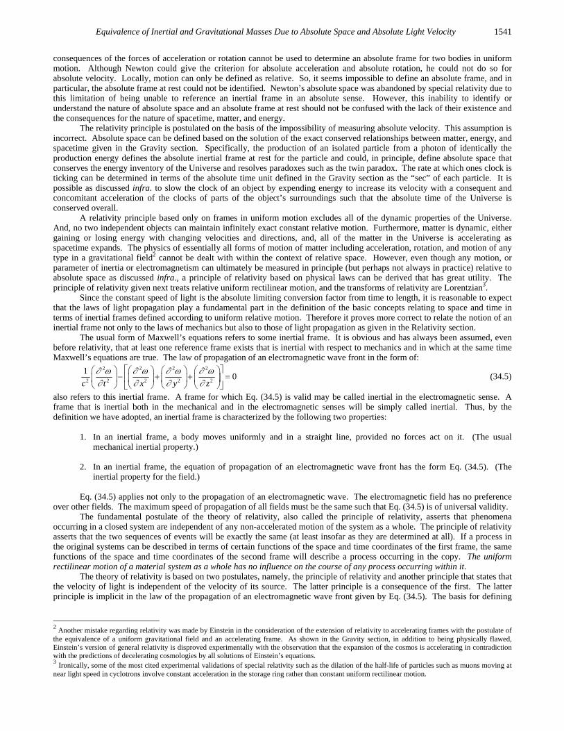
Equivalence of Inertial and Gravitational Masses Due to Absolute Space and Absolute Light Velocity 1541
consequences of the forces of acceleration or rotation cannot be used to determine an absolute frame for two bodies in uniform motion. Although Newton could give the criterion for absolute acceleration and absolute rotation, he could not do so for absolute velocity. Locally, motion can only be defined as relative. So, it seems impossible to define an absolute frame, and in particular, the absolute frame at rest could not be identified. Newton’s absolute space was abandoned by special relativity due to this limitation of being unable to reference an inertial frame in an absolute sense. However, this inability to identify or understand the nature of absolute space and an absolute frame at rest should not be confused with the lack of their existence and the consequences for the nature of spacetime, matter, and energy.
The relativity principle is postulated on the basis of the impossibility of measuring absolute velocity. This assumption is incorrect. Absolute space can be defined based on the solution of the exact conserved relationships between matter, energy, and spacetime given in the Gravity section. Specifically, the production of an isolated particle from a photon of identically the production energy defines the absolute inertial frame at rest for the particle and could, in principle, define absolute space that conserves the energy inventory of the Universe and resolves paradoxes such as the twin paradox. The rate at which ones clock is ticking can be determined in terms of the absolute time unit defined in the Gravity section as the “sec” of each particle. It is possible as discussed infra. to slow the clock of an object by expending energy to increase its velocity with a consequent and concomitant acceleration of the clocks of parts of the object’s surroundings such that the absolute time of the Universe is conserved overall.
A relativity principle based only on frames in uniform motion excludes all of the dynamic properties of the Universe. And, no two independent objects can maintain infinitely exact constant relative motion. Furthermore, matter is dynamic, either gaining or losing energy with changing velocities and directions, and, all of the matter in the Universe is accelerating as spacetime expands. The physics of essentially all forms of motion of matter including acceleration, rotation, and motion of any type in a gravitational field2 cannot be dealt with within the context of relative space. However, even though any motion, or parameter of inertia or electromagnetism can ultimately be measured in principle (but perhaps not always in practice) relative to absolute space as discussed infra., a principle of relativity based on physical laws can be derived that has great utility. The principle of relativity given next treats relative uniform rectilinear motion, and the transforms of relativity are Lorentzian3.
Since the constant speed of light is the absolute limiting conversion factor from time to length, it is reasonable to expect that the laws of light propagation play a fundamental part in the definition of the basic concepts relating to space and time in terms of inertial frames defined according to uniform relative motion. Therefore it proves more correct to relate the notion of an inertial frame not only to the laws of mechanics but also to those of light propagation as given in the Relativity section.
The usual form of Maxwell’s equations refers to some inertial frame. It is obvious and has always been assumed, even before relativity, that at least one reference frame exists that is inertial with respect to mechanics and in which at the same time Maxwell’s equations are true. The law of propagation of an electromagnetic wave front in the form of:
2 2 2 2
2 2 2 2 2
10
c t x y z
(34.5)
also refers to this inertial frame. A frame for which Eq. (34.5) is valid may be called inertial in the electromagnetic sense. A frame that is inertial both in the mechanical and in the electromagnetic senses will be simply called inertial. Thus, by the definition we have adopted, an inertial frame is characterized by the following two properties:
1. In an inertial frame, a body moves uniformly and in a straight line, provided no forces act on it. (The usual mechanical inertial property.)
2. In an inertial frame, the equation of propagation of an electromagnetic wave front has the form Eq. (34.5). (The
inertial property for the field.)
Eq. (34.5) applies not only to the propagation of an electromagnetic wave. The electromagnetic field has no preference over other fields. The maximum speed of propagation of all fields must be the same such that Eq. (34.5) is of universal validity.
The fundamental postulate of the theory of relativity, also called the principle of relativity, asserts that phenomena occurring in a closed system are independent of any non-accelerated motion of the system as a whole. The principle of relativity asserts that the two sequences of events will be exactly the same (at least insofar as they are determined at all). If a process in the original systems can be described in terms of certain functions of the space and time coordinates of the first frame, the same functions of the space and time coordinates of the second frame will describe a process occurring in the copy. The uniform rectilinear motion of a material system as a whole has no influence on the course of any process occurring within it.
The theory of relativity is based on two postulates, namely, the principle of relativity and another principle that states that the velocity of light is independent of the velocity of its source. The latter principle is a consequence of the first. The latter principle is implicit in the law of the propagation of an electromagnetic wave front given by Eq. (34.5). The basis for defining
2 Another mistake regarding relativity was made by Einstein in the consideration of the extension of relativity to accelerating frames with the postulate of the equivalence of a uniform gravitational field and an accelerating frame. As shown in the Gravity section, in addition to being physically flawed, Einstein’s version of general relativity is disproved experimentally with the observation that the expansion of the cosmos is accelerating in contradiction with the predictions of decelerating cosmologies by all solutions of Einstein’s equations. 3 Ironically, some of the most cited experimental validations of special relativity such as the dilation of the half-life of particles such as muons moving at near light speed in cyclotrons involve constant acceleration in the storage ring rather than constant uniform rectilinear motion.

Chapter 34 1542
inertial reference frames is Eq. (34.5) together with the fact of the uniform rectilinear motion of a body not subject to forces. The principle of relativity holds in the case that the reference frames are inertial.
It is appropriate to give a generalized interpretation of the law of wave front propagation and to formulate the following general postulate:
There exists a maximum speed for the propagation of any kind of action—the speed of light in free space.
This principle is very significant because the transmission of signals with greatest possible speed plays a fundamental part in the definition of concepts concerning space and time. The very notion of a definite frame of reference for describing events in space and time depends on the existence of such signals. The principle formulated above, by asserting the existence of a general upper limit for all kinds of action and signal, endows the speed of light with a universal significance, independent of the particular properties of the agency of transmission and reflecting a certain objective property of spacetime. This principle has a logical connection with the principle of relativity. For if there was no single limiting velocity, but instead different agents, e.g. light and gravitation, propagated in vacuum with different speeds, then the principle of relativity would necessarily be violated as regards at least one of the agents. The principle of the universal limiting velocity can be made mathematically precise as follows:
For any kind of wave advancing with limiting velocity and capable of transmitting signals, the equation of front
propagation is the same as the equation for the front of a light wave.
Thus, the equation:
2
22 2
10grad
c t
(34.6)
acquires a general character; it is more general than Maxwell’s equations from which Maxwell originally derived it. As a consequence of the principle of the existence of a universal limiting velocity one can assert the following: the differential equations describing any field that is capable of transmitting signals must be of such a kind that the equation of their characteristics is the same as the equation for the characteristics of light waves. In addition to governing the propagation of any form of energy, the wave equation governs fundamental particles created from energy and vice versa, the associated effects of mass on spacetime, and the evolution of the Universe itself. Specially, the equation that describes the electron dynamics of the rotational energy and angular momentum with 0 given by Eqs. (1.56-1.65) is the wave equation, the relativistic correction of spacetime due to particle production travels according to the wave equation as given in the Gravity section, and the evolution of the Universe is according to the wave equation as given in the Gravity section and the Unification of Spacetime, the Forces, Matter, and Energy section (Eqs. (33.45-33.46)). RELATIONSHIP OF THE PROPERTIES OF SPACETIME AND THE PHOTON TO THE INERTIAL AND GRAVITATIONAL MASSES LORENTZ TRANSFORMS BASED ON CONSTANT RELATIVE VELOCITY The magnetic force was unified with the Coulombic force by Maxwell. Lorentz derived the transformations named after him which formalize the origin of the magnetic force as a relativistic correction of the Coulomb force. The unification of electricity and magnetism by Maxwell permitted him to derive a wave equation, which predicted the propagation of electromagnetic waves at the speed of light (Eq. (34.1)). Maxwell’s wave equation defines a four-dimensional spacetime with the speed of light as a maximum permitted according to the permeability and permittivity of spacetime. Minkowski originated the concept of a four-dimensional spacetime formally expressed as the Minkowski tensor [6]. The Minkowski tensor corresponds to the electromagnetic wave equation derived by Maxwell and can be derived from it [7]. Special relativity is implicit in the wave equation of electromagnetic waves that travel at the speed of light. The generalization of this metric to mass as well as charge requiring application of Lorentz transformations to relative parameters comprises the theory of special relativity. The Lorentz transformations quantify the measurement of the increase in mass, length contraction, and time dilation in the direction of constant relative motion of separate inertial frames due to the finite maximum speed of light.
Using the principle that that light velocity is the constant maximum c in all inertial frames, the relationships between distances in two frames with one moving a constant velocity relative to the other are shown in the Relativity section to be [8] :
2 2
202 2
t tc L v
(34.7)
0
2
2
2
1
L
ctvc
(34.8)

Equivalence of Inertial and Gravitational Masses Due to Absolute Space and Absolute Light Velocity 1543
0
2
21
tt
vc
(34.9)
The Lorentz transformation of the other spatial-temporal and mechanical parameters that maintain the covariance of mechanical laws gives the following relationships between the parameters of inertial frames [8]:
2
0 21
vl l
c (34.10)
0
2
21
mm
vc
(34.11)
0
2
21
m vp
vc
(34.12)
Using the Lorentz transformation of the energy of particle production given by Eq. (34.49) gives:
2
2 0
2
21
m cE mc
vc
(34.13)
Squaring the energy given in Eq. (34.13) gives:
2 4
2 02
21
m cE
vc
(34.14)
The square of the Lorentz momentum given by Eq. (34.12) multiplied by 2c is:
2 2 2
2 2 02
21
m v cp c
vc
(34.15)
Subtracting 2 2p c from 2E gives:
22 40 22 4 2 2 2
2 2 2 2 40 002 2
2 2
1
1 1
vm c
cm c m v cE p c m c
v vc c
(34.16)
Thus, 2 2 4 2 2
0E m c p c (34.17)
MINKOWSKI SPACE When speaking of the relativity of a frame of reference or simply of relativity, one usually means that there exist identical physical processes in different frames of reference. According to the generalized Galilean principle of relativity, identical processes are possible in all inertial frames of reference related by Lorentz transformations. On the other hand, Lorentz transformations characterize the uniformity of Galilean spacetime. Using the four-dimensional coordinates x for describing the events and the world-line in spacetime the separation of proper time between two events x and x dx is:
2d g dx dx (34.18)
where g is the metric tensor which determines the geometric character of spacetime. For different coordinate systems, the
dx may not be the same, but the separation 2d remains unchanged. The metric g for Euclidean space called the
Minkowski tensor is:
2
2
2
1 0 0 0
10 0 0
10 0 0
10 0 0
c
c
c
(34.19)
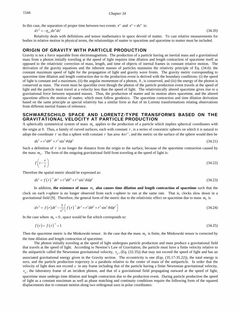
Chapter 34 1544
In this case, the separation of proper time between two events x and x dx is: 2d dx dx
(34.20)
Relativity deals with definitions and tensor mathematics in space devoid of matter. To cast relative measurements for bodies in relative motion in physical terms, the relationships of matter to spacetime and spacetime to matter must be included.
ORIGIN OF GRAVITY WITH PARTICLE PRODUCTION Gravity is not a force separable from electromagnetism. The production of a particle having an inertial mass and a gravitational mass from a photon initially traveling at the speed of light requires time dilation and length contraction of spacetime itself as opposed to the relativistic correction of mass, length, and time of objects of inertial frames in constant relative motion. The derivation of the gravity equations and the inherent masses of particles maintains the relativity principle of Eq. (34.6): the constant maximum speed of light for the propagation of light and gravity wave fronts. The gravity metric corresponding to spacetime time dilation and length contraction due to the production event is derived with the boundary conditions: (i) the speed of light is constant and a maximum, (ii) the angular momentum of a photon, , is conserved, and (iii) the energy of the photon is conserved as mass. The event must be spacelike even though the photon of the particle production event travels at the speed of light and the particle must travel at a velocity less than the speed of light. The relativistically altered spacetime gives rise to a gravitational force between separated masses. Thus, the production of matter and its motion alters spacetime, and the altered spacetime affects the motion of matter, which must follow geodesics. The spacetime contraction and time dilation derivation based on the same principle as special relativity has a similar form as that of its Lorentz transformations relating observations from different inertial frames of reference. SCHWARZSCHILD SPACE AND LORENTZ-TYPE TRANSFORMS BASED ON THE GRAVITATIONAL VELOCITY AT PARTICLE PRODUCTION A spherically symmetrical system of mass 0m applies to the production of a particle which implies spherical coordinates with
the origin at 0. Thus, a family of curved surfaces, each with constant r , is a series of concentric spheres on which it is natural to adopt the coordinate r so that a sphere with constant r has area 24 r , and the metric on the surface of the sphere would then be
2 2 2 2 2 2sinds r d r d (34.21)
Such a definition of r is no longer the distance from the origin to the surface, because of the spacetime contraction caused by the mass 0m . The form of the outgoing gravitational field front traveling at the speed of light is:
r
f tc
(34.22)
Therefore the spatial metric should be expressed as:
12 2 2 2 2 2 2sinds f r dr r d r d (34.23)
In addition, the existence of mass 0m also causes time dilation and length contraction of spacetime such that the
clock on each r-sphere is no longer observed from each r-sphere to run at the same rate. That is, clocks slow down in a gravitational field [9]. Therefore, the general form of the metric due to the relativistic effect on spacetime due to mass 0m is
12 2 2 2 2 2 2 22
1sind f r dt f r dr r d r d
c (34.24)
In the case where 0 0m , space would be flat which corresponds to:
11f r f r
(34.25)
Then the spacetime metric is the Minkowski tensor. In the case that the mass 0m is finite, the Minkowski tensor is corrected by
the time dilation and length contraction of spacetime. The photon initially traveling at the speed of light undergoes particle production and must produce a gravitational field
that travels at the speed of light. According to Newton’s Law of Gravitation, the particle must have a finite velocity relative to the antiparticle called the Newtonian gravitational velocity, gv , (Eq. (32.35)) that may not exceed the speed of light and has an
associated gravitational energy given in the Gravity section. The eccentricity is one (Eqs. (35.17-35.22)), the total energy is zero, and the particle production trajectory is a parabola relative to the center of mass of the antiparticle. In order that the velocity of light does not exceed c in any frame including that of the particle having a finite Newtonian gravitational velocity,
gv , the laboratory frame of an incident photon, and that of a gravitational field propagating outward at the speed of light,
spacetime must undergo time dilation and length contraction due to the production event. During particle production the speed of light as a constant maximum as well as phase matching and continuity conditions require the following form of the squared displacements due to constant motion along two orthogonal axes in polar coordinates:

Equivalence of Inertial and Gravitational Masses Due to Absolute Space and Absolute Light Velocity 1545
22 2
gc v t ct (34.26)
2
2 2 1 gvt
c
(34.27)
Thus,
2
1 gvf r
c
(34.28)
The derivation and result of spacetime time dilation is analogous to the derivation and result of special relativistic time dilation given by Eqs. (31.11-31.15) wherein the gravitational velocity replaces the relative velocity of two inertial frames in the Lorentz factor. The general form of the metric due to the relativistic effect on spacetime due to mass 0m is:
12 2
2 2 2 2 2 2 2 22
11 1 sing gv v
d dt dr r d r dc c c
(34.29)
The equivalence of the gravitational and inertial masses, according to experiments and Eqs. (34.49) and (34.67-34.68), prove that Newton’s Gravitational Law is exact on a local scale. The correction to Newton’s Gravitational Law due to the relativistic effect of the presence of mass on spacetime may be determined by substitution of the gravitational escape velocity,
gv , given by:
0 02 2g
C
Gm Gmv
r
(34.30)
into Eq. (34.29) for gv . The corresponding Newtonian gravitational radius is given by [10]:
02
2g
Gmr
c (34.31)
Thus, Eq. (34.29) can also be expressed as:
1
2 2 2 2 2 2 2 22
11 1 sing gr r
d dt dr r d r dr c r
(34.32)
In the case of the boundary conditions of Eqs. (34.48-34.49), Eq. (34.30) and Eq. (34.31), three families of leptons and quarks are predicted in the corresponding sections wherein each particle corresponds to a unique atomic orbital radius equal to its Compton wavelength bar. At particle production, a photon having a radius and a wavelength equal to the Compton wavelength bar of the particle forms a transition state atomic orbital of the particle of the same wavelength.
*Cr r
mc (34.33)
The resulting metric g for non-Euclidean space due to the relativistic effect on spacetime due to mass 0m with gv
given by Eq. (34.30) is
02
1
02 2
22
2 22
21 0 0 0
210 1 0 0
10 0 0
10 0 0 sin
Gm
c r
Gm
c c rg
rc
rc
(34.34)
In this case, the separation of proper time between two events x and x dx is:
1
2 2 2 2 2 2 2 20 02 2 2
2 211 1 sin
Gm Gmd dt dr r d r d
c r c c r
(34.35)
The Schwarzschild-type metric (Eq. (34.35)) gives the relationship whereby matter causes relativistic corrections to spacetime that determines the curvature of spacetime and is the origin of gravity.

Chapter 34 1546
The origin of gravity is fundamental particles, and the masses and fields from particles superimpose. So, 0m , the mass of a
fundamental particle, may be replaced by M , the sum of the masses of the particles which make up a massive body. In this case, Eq. (34.35) is equivalent to a modified version of the Schwarzschild metric that is conservative of matter, energy, and
spacetime and lacking the reduced radial coordinate, 2
GMr
c , and singularity issues of general relativity.
The Schwarzschild metric provides transforms of the spacetime and mass-energy parameters based on the effect of gravity in an analogous manner as the Minkowski tensor provides the Lorentz transforms for the corresponding inertial parameters. As shown in Eq. (32.70), the relativistic correction for time is:
2
21 g
tv
c
(34.36)
Then,
2
21 g
o
vl l
c (34.37)
The spacetime corrections have the same form as the special relativistic corrections for time and length with gv in place of v .
Consider the relationship between proper and coordinate mass derived in the Gravity section by considering an object of mass m orbiting an object of mass M . The gravitational force is central; thus the angular momentum is constant. Consider that a radial force is applied to increase the radius r of the object’s orbit with a change of its energy E . The angular momentum is conserved; thus,
2 2i f
i f
d dmr mr
dt dt
(34.38)
where i
d
dt
is the initial angular velocity, f
d
dt
is the final angular velocity, ir is the initial radius and fr is the final radius.
At fixed radius, 2dr is zero, but 2dt is finite. Applying the time relativistic correction given by Eq. (34.35) and Eqs. (34.26-34.28) gives the mass fm at fr with respect to the mass im of the inertial frame of ir as:
2
21i f
GMm m
rc
(34.39)
where r is the increase in the radius. The proper energy pE of the object is given by:
22
21i p
GMm c E
rc
(34.40)
The relativistic correction for energy is of the same form as the special relativistic correction for mass (Eq. (31.21)) with gv in
place of v .
2
2
1
p
g
Emc
v
c
(34.41)
where m is the coordinate mass of the orbiting body and E is the energy of the orbiting object. In the case that the gravitational velocity is much less than the speed of light ( gv c ), the gravitational energy gE converges to that given by Newton’s law of
Gravitation.
22
1 21
2p
GME mc
rc
(34.42)
2p
GMmE mc
r (34.43)
g
GMmE
r (34.44)

Equivalence of Inertial and Gravitational Masses Due to Absolute Space and Absolute Light Velocity 1547
PARTICLE PRODUCTION CONTINUITY CONDITIONS FROM MAXWELL’S EQUATIONS, AND THE SCHWARZSCHILD METRIC GIVE RISE TO CHARGE, MOMENTUM AND MASS The photon possesses electric and magnetic fields and the corresponding energies and momentum. The angular momentum of the photon given by:
41Re ( )
8dx
c m r E B* (34.45)
in the Photon section is conserved [11] during particle production. The energy due to the angular frequency of the photon according to Planck’s equation and those of its electric and magnetic fields match those of the particle to which it gives rise. The transition state has dimensions of the particle’s Compton wavelength bar such that the speed matches light speed at the photon’s frequency as a further constraint of Maxwell’s equations and the inherent special relativity. This limiting speed is set by the permittivity and permeability of spacetime. Spacetime undergoes time dilation and length contraction at the particle production event as a gravitation-field front propagates out as a light-wave front at light speed. The photon’s effect on spacetime and spacetime’s effect on the corresponding production particle then determine its inertial and gravitational mass 0m
and the fundamental charge e where the momentum and energies of the photon are continuous with those of the particle during the production event.
The photon to particle event requires a transition state that is continuous wherein the velocity of a transition state atomic orbital is the speed of light. The radius, r , is the Compton wavelength bar, C , given by Eq. (34.33). At production, the Planck
equation energy, the electric potential energy, and the magnetic energy are equal to 20m c .
The Schwarzschild metric gives the relationship whereby matter causes relativistic corrections to spacetime that determines the masses of fundamental particles. Substitution of Cr ; 0dr ; 0d ; 2sin 1 into the Schwarzschild
metric gives:
12 2
02 * 2
21
Gm vd dt
c r c
(34.46)
with 2 2v c , the relationship between the proper time and the coordinate time is:
2 * 2
2 2 g
c
vGM GMti ti ti
c r c c
(34.47)
When the atomic orbital velocity is the speed of light, continuity conditions based on the constant maximum speed of light given by Maxwell’s equations are mass energy = Planck equation energy = electric potential energy = magnetic energy = mass/spacetime metric energy. Therefore,
2 *o mag spacetimem c V E E (34.48)
2 2 22 22 * 1 1 0
0 22 30 0 0
4 1 sec 22C
C C C
e ce hm c
m Gmm
(34.49)
The continuity conditions based on the constant maximum speed of light given by the Schwarzschild metric are:
2
proper time gravitational wave condition gravitational mass phase matching
coordinate time electromagnetic wave condition charge/inertial mass phase matching
2
proper time
coordinate timegC
Gmvc
i ic
(34.50)
Each of the Planck equation energy, electric energy, and magnetic energy corresponds to a particle given by the relationship between the proper time and the coordinate time. The electron and down-down-up neutron correspond to the Planck equation energy. The muon and strange-strange-charmed neutron correspond to the electric energy. The tau and bottom-bottom-top neutron correspond to the magnetic energy. The particle must possess the escape velocity gv relative to the
antiparticle where gv c . According to Newton’s law of gravitation, the eccentricity is one and the particle production
trajectory is a parabola relative to the center of mass of the antiparticle. The masses of the three families of leptons and quarks are given in the corresponding sections. Exemplary relations between fundamental particles are shown in Table 34.1.

Chapter 34 1548
Table 34.1. The calculated relations between the lepton masses and neutron to electron mass ratio are given in terms of the dimensionless fine structure constant only and compared to experimental values from the 1998 CODATA and the Particle Data Group given in parentheses [12-13].
2
22 3
1 22
206.768282 1
2e
m
m
(206.76827)
21 3
2
12
16.8172 1 4
m
m
(16.817)
2
23 3
2
1 22
3477.24 1 4e
m
m
(3477.3)
2
2
2
1 2212 3
1838.671
1 22
N
e
m
m
(1838.68)
Consider pair production. The proper time of the particle is equated with the coordinate time according to the Schwarzschild metric corresponding to light speed. The special relativistic condition corresponding to the Planck energy (Eq. (34.49)) gives the mass of the electron [12-13]:
2
2 2
22 sec
Gm
mc c
(34.51)
1 1
2 431
29.0998 10
sec 2e
h cm X kg
c G
(34.52)
where 31 experimental 9.10945455 10em X kg . A clock is defined in terms of a self-consistent system of units used to measure the
particle mass. Presently the second is defined as the time required for 9,192,631,770 vibrations within the cesium-133 atom. The “sec” as defined in Eqs. (34.49) and (34.51) is a fundamental constant, namely, the metric of spacetime (it is almost identically equal to the present value of the MKS second for reasons explained in the Gravity section). A unified theory can only provide the relationships between all measurable observables in terms of a clock defined in terms of fundamental constants according to those observables and used to measure them. The so defined “clock” measures “clicks” on an observable in one aspect, and in another, it is the ruler of spacetime of the Universe with the implicit dependence of spacetime on matter-energy conversion as shown in the Gravity and Relationship of Matter to Energy and Spacetime Expansion sections.

Equivalence of Inertial and Gravitational Masses Due to Absolute Space and Absolute Light Velocity 1549
RELATIONSHIP OF MATTER TO ENERGY AND SPACETIME EXPANSION The Schwarzschild metric gives the relationship whereby matter causes relativistic corrections to spacetime. The limiting velocity c results in the contraction of spacetime due to particle production, which is given by 2 gr where gr is the
gravitational radius of the particle. This has implications for the expansion of spacetime when matter converts to energy. Q the mass/energy to expansion/contraction quotient of spacetime is given by the ratio of the mass of a particle at production divided by T , the period of production where:
3
340 0 0
02
3.22 102 2 4 sec2g
m m m c kgQ X
r GmT Gcc
c
(34.53)
The gravitational equations with the equivalence of the particle production energies (Eq. (34.49)) permit the conservation of
mass/energy ( 2E mc ) and spacetime (3
34 3.22 10
4 sec
c kgX
G ). With the conversion of 343.22 10 gX k of matter to energy,
spacetime expands by 1 sec. The photon has inertial mass and angular momentum, but due to Maxwell’s equations and the implicit special relativity it does not have a gravitational mass. The observed gravitational deflection of light is predicted as given in the Gravity section. COSMOLOGICAL CONSEQUENCES The Universe is closed (it is finite but with no boundary). It is a 3-sphere Universe-Riemannian three-dimensional hyperspace plus time of constant positive curvature at each r-sphere. The Universe is oscillatory in matter/energy and spacetime with a finite minimum radius, the gravitational radius. Spacetime expands as mass is released as energy which provides the basis of the atomic, thermodynamic, and cosmological arrows of time. Different regions of space are isothermal even though they are separated by greater distances than that over which light could travel during the time of the expansion of the Universe [14]. Presently, stars and large scale structures exist which are older than the elapsed time of the present expansion as stellar, galaxy, and supercluster evolution occurred during the contraction phase [15–21]. The maximum power radiated by the Universe, which
occurs at the beginning of the expansion phase, is 5
51 2.89 10
4U
cP X W
G . Observations beyond the beginning of the
expansion phase are not possible since the Universe was entirely matter filled. THE PERIOD OF OSCILLATION OF THE UNIVERSE BASED ON CLOSED PROPAGATION OF LIGHT Mass/energy is conserved during harmonic expansion and contraction. The gravitational potential energy gravE given by Eq.
(32.148) with 0 Um m is equal to 2Um c when the radius of the Universe r is the gravitational radius Gr (Eq. (32.22)). The
gravitational velocity Gv (Eq. (32.33) with Gr r and 0 Um m ) is the speed of light in a circular orbit wherein the eccentricity
is equal to zero and the escape velocity from the Universe can never be reached. The period of the oscillation of the Universe and the period for light to transverse the Universe corresponding to the gravitational radius Gr must be equal. The harmonic
oscillation period, T , is:
54
3 3
19 11
2 2 10 2 2
3.10 10 sec 9.83 10 ears
G UG X kgr Gm
Tc c c
X X y
(34.54)
where the mass of the Universe, Um , is approximately 54 2 10X kg . (The initial mass of the Universe of 54
2 10X kg is based
on internal consistency with the size, age, Hubble constant, temperature, density of matter, and power spectrum.) Thus, the observed Universe will expand as mass is released as photons for 11
4.92 10X years . At this point in its world line, the Universe will obtain its maximum size and begin to contract.

Chapter 34 1550
THE DIFFERENTIAL EQUATION OF THE RADIUS OF THE UNIVERSE Based on conservation of mass/energy ( 2E mc ) and spacetime (
334
3.22 104 sec
c kgX
G ), the Universe behaves as a simple
harmonic oscillator having a restoring force, F , which is proportional to the radius. The proportionality constant, k , is given in terms of the potential energy, E , gained as the radius decreases from the maximum expansion to the minimum contraction.
2
Ek
(34.55)
Since the gravitational potential energy gravE is equal to 2Um c when the radius of the Universe r is the gravitational radius Gr
2 2
22
2
U U
G U
m c m cF k
r Gmc
(34.56)
and, considering the oscillation, the differential equation of the radius of the Universe, is:
2 2
22
2
0U UU U
G U
m c m cm m
r Gmc
(34.57)
The maximum radius of the Universe, the amplitude, or , of the time harmonic variation in the radius of the Universe, is
given by the quotient of the total mass of the Universe and Q (Eq. (34.53)), the mass/energy to expansion/contraction quotient.
54
12 0 3 3
2 10 1.97 10
4 4
U Um m X kgr X light years
c cQG G
(34.58)
The minimum radius which corresponds to the gravitational radius, gr , given by Eq. (32.36) with 0 Um m is
27 11
2
22.96 10 3.12 10 U
g
Gmr X m X light years
c (34.59)
When the radius of the Universe is the gravitational radius, gr , the proper time is equal to the coordinate time by Eq. (34.47),
and the gravitational escape velocity gv of the Universe is the speed of light. The radius of the Universe as a function of time is
3 32
3
22 2cos cos
2 2
4 4
U U U U Ug
G U
cm cm Gm cm cmt tr
r Gmc cQ Q cc cG G
(34.60)
As shown in the Gravity section, Eq. (34.60) correctly predicts the observed size, age, Hubble constant, temperature, density of matter, power spectrum, large-scale structure, and acceleration rate of the expansion of the Universe. The latter astonishing observation was predicted years before it was observed [22]. THE PERIODS OF SPACETIME EXPANSION/CONTRACTION AND PARTICLE DECAY/PRODUCTION FOR THE UNIVERSE ARE EQUAL The period of the expansion/contraction cycle of the radius of the Universe, T , is given by Eq. (34.54). It follows from the Poynting power theorem with spherical radiation that the transition lifetimes are given by the ratio of energy and the power of the transition (Eq. (33.35)). Exponential decay applies to electromagnetic energy decay,
2
( )tt Th t e u t e u t
(34.61)
The coordinate time is imaginary because energy transitions are spacelike due spacetime expansion from matter to energy conversion. For example, the mass of the electron (a fundamental particle) is given by:
12 2sec
2C C
ge
C
ivGm
(34.62)
where gv is Newtonian gravitational velocity (Eq. (34.30)). When the gravitational radius gr is the radius of the Universe, the
proper time is equal to the coordinate time by Eq. (34.47), and the gravitational escape velocity gv of the Universe is the speed
of light. Replacement of the coordinate time, t , by the spacelike time, it , gives:
2 2
( ) Re cosi t
Th t e tT
(34.63)

Equivalence of Inertial and Gravitational Masses Due to Absolute Space and Absolute Light Velocity 1551
where the period is T (Eq. (34.54)). The continuity conditions based on the constant maximum speed of light (Maxwell’s equations) are given by Eqs. (34.48-34.49). The continuity conditions based on the constant maximum speed of light (Schwarzschild metric) are given by Eq. (34.50). The periods of spacetime expansion/contraction and particle decay/production for the Universe are equal because only the particles which satisfy Maxwell’s equations and the relationship between proper time and coordinate time imposed by the Schwarzschild metric may exist.
The general form of the light front wave equation is given by Eq. (34.5). The equation of the radius of the Universe, , may be written as:
3 32
3
2 2cos
2
4 4
U U U
U
Gm cm cmt
Gmc cc ccG G
(34.64)
which is a solution of the wave equation for a light wave front. Maxwell’s equations, Planck’s equation, the de Broglie equation, Newton’s laws, and special relativity, and gravity are unified. Classical physical laws apply on all scales wherein space is finite-absolute rather than infinite-relative4.
EQUIVALENCE OF THE GRAVITATIONAL AND INERTIAL MASSES The relationships of relativity and gravity have the same form with the interchange of the inertial and gravitational velocities (Compare Eqs. (34.7-34.17) with Eqs. (34.26), and (34.36-34.41)). The relationships are reciprocal due to the nature of absolute space that is produced or annihilated with particle annihilation or production, respectively. Due to the finite propagation time for signals set by the speed of light which is in turn set by the finite permeability and permittivity of free space the mechanics parameters are corrected by Lorentz transformations or their equivalent with the gravitational velocity replacing the constant kinetic velocity in the case of gravitating bodies.
Extensive experimentation dating from Galileo Galilei’s Pisa experiment to the present has shown that irrespective of the object chosen, the acceleration of an object produced by the gravitational force is the same, which from Eq. (32.4) implies that the value of /g im m should be the same for all objects. In other words, we have:
universal constantg
i
m
m (34.65)
the equivalence of the gravitational mass and the inertial mass. The fractional deviation of Eq. (34.65) from a constant is experimentally confirmed to less 111 10X [23]. The equivalence of the gravitational mass and the inertial mass is a conservation statement of the mass, energy, and spacetime of the Universe. The overall inventory is a constant with the inter-conversion related by the ratios of fundamental constants of spacetime.
At particle production, the outgoing gravitational field, traveling as a wave front, carries the change in the curvature of spacetime. The front must travel at light speed since the permittivity 0 and permeability 0 of free spacetime are and must
remain independent of curvature in order for the laws of physics to be covariant and the physics of the Universe to be conservative. Thus, any perturbation must travel at the speed of light c given by Eq. (34.1). The justification for Eq. (34.26) is the relativity principle based on Eq. (34.6) and the invariance of the light speed due to the invariance of the permittivity 0 and
permeability 0 of free spacetime.
From Eqs. (34.35) and (34.47-34.53), each r-sphere of the Universe comprising a finite, closed 3-sphere Universe-(Riemannian three-dimensional hyperspace plus time of constant positive curvature at each r-sphere) is determined by a clock
set by the conservation relationship of mass-energy, 2E mc , and spacetime, 3
34 3.22 10
4 sec
c kgX
G . Spacetime expands at
light speed as mass is released as energy which provides the basis of the atomic, thermodynamic, and cosmological arrows of time.
Consider the relationship (Eq. (34.41)) between gravitational mass gm and proper energy pE of a gravitating object
based on the absolute light speed and absolute space:
2
2
1
pg
g
Em c
v
c
(34.66)
4 The views that all phenomena in the universe are purely relative, the basis of gravity is the equivalence principle, and light has a wave-particle duality nature determined by the act of measurement were the seeds for the abandonment of the testable physical laws of Newton and Maxwell. Subsequent missteps of the interpretation of the electron as a nonphysical point-particle probability wave with intrinsic spin, the use of mathematics for circumventing intrinsic infinites while engendering the vacuum with infinities of virtual particles, and the pursuit of compactified extra dimensions, nonbaryonic dark matter and dark energy gave rise to the pure mathematics and the metaphysics of current quantum mechanics and string theory. This path has been a complete failure at achieving the goal of unification of the forces and laws of nature.
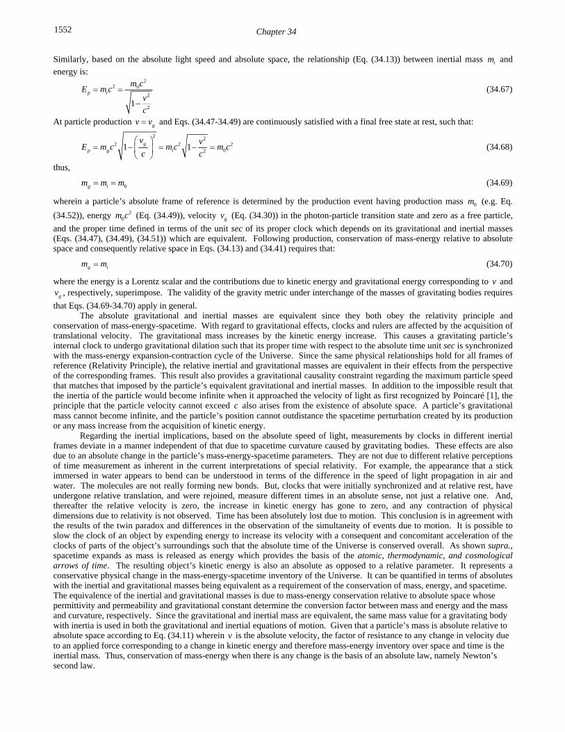
Chapter 34 1552
Similarly, based on the absolute light speed and absolute space, the relationship (Eq. (34.13)) between inertial mass im and
energy is:
2
2 0
2
21p i
m cE m c
vc
(34.67)
At particle production gv v and Eqs. (34.47-34.49) are continuously satisfied with a final free state at rest, such that:
2 2
2 2 202
1 1gp g i
v vE m c m c m c
c c
(34.68)
thus,
0g im m m (34.69)
wherein a particle’s absolute frame of reference is determined by the production event having production mass 0m (e.g. Eq.
(34.52)), energy 20m c (Eq. (34.49)), velocity gv (Eq. (34.30)) in the photon-particle transition state and zero as a free particle,
and the proper time defined in terms of the unit sec of its proper clock which depends on its gravitational and inertial masses (Eqs. (34.47), (34.49), (34.51)) which are equivalent. Following production, conservation of mass-energy relative to absolute space and consequently relative space in Eqs. (34.13) and (34.41) requires that:
g im m (34.70)
where the energy is a Lorentz scalar and the contributions due to kinetic energy and gravitational energy corresponding to v and
gv , respectively, superimpose. The validity of the gravity metric under interchange of the masses of gravitating bodies requires
that Eqs. (34.69-34.70) apply in general. The absolute gravitational and inertial masses are equivalent since they both obey the relativity principle and
conservation of mass-energy-spacetime. With regard to gravitational effects, clocks and rulers are affected by the acquisition of translational velocity. The gravitational mass increases by the kinetic energy increase. This causes a gravitating particle’s internal clock to undergo gravitational dilation such that its proper time with respect to the absolute time unit sec is synchronized with the mass-energy expansion-contraction cycle of the Universe. Since the same physical relationships hold for all frames of reference (Relativity Principle), the relative inertial and gravitational masses are equivalent in their effects from the perspective of the corresponding frames. This result also provides a gravitational causality constraint regarding the maximum particle speed that matches that imposed by the particle’s equivalent gravitational and inertial masses. In addition to the impossible result that the inertia of the particle would become infinite when it approached the velocity of light as first recognized by Poincaré [1], the principle that the particle velocity cannot exceed c also arises from the existence of absolute space. A particle’s gravitational mass cannot become infinite, and the particle’s position cannot outdistance the spacetime perturbation created by its production or any mass increase from the acquisition of kinetic energy.
Regarding the inertial implications, based on the absolute speed of light, measurements by clocks in different inertial frames deviate in a manner independent of that due to spacetime curvature caused by gravitating bodies. These effects are also due to an absolute change in the particle’s mass-energy-spacetime parameters. They are not due to different relative perceptions of time measurement as inherent in the current interpretations of special relativity. For example, the appearance that a stick immersed in water appears to bend can be understood in terms of the difference in the speed of light propagation in air and water. The molecules are not really forming new bonds. But, clocks that were initially synchronized and at relative rest, have undergone relative translation, and were rejoined, measure different times in an absolute sense, not just a relative one. And, thereafter the relative velocity is zero, the increase in kinetic energy has gone to zero, and any contraction of physical dimensions due to relativity is not observed. Time has been absolutely lost due to motion. This conclusion is in agreement with the results of the twin paradox and differences in the observation of the simultaneity of events due to motion. It is possible to slow the clock of an object by expending energy to increase its velocity with a consequent and concomitant acceleration of the clocks of parts of the object’s surroundings such that the absolute time of the Universe is conserved overall. As shown supra., spacetime expands as mass is released as energy which provides the basis of the atomic, thermodynamic, and cosmological arrows of time. The resulting object’s kinetic energy is also an absolute as opposed to a relative parameter. It represents a conservative physical change in the mass-energy-spacetime inventory of the Universe. It can be quantified in terms of absolutes with the inertial and gravitational masses being equivalent as a requirement of the conservation of mass, energy, and spacetime. The equivalence of the inertial and gravitational masses is due to mass-energy conservation relative to absolute space whose permittivity and permeability and gravitational constant determine the conversion factor between mass and energy and the mass and curvature, respectively. Since the gravitational and inertial mass are equivalent, the same mass value for a gravitating body with inertia is used in both the gravitational and inertial equations of motion. Given that a particle’s mass is absolute relative to absolute space according to Eq. (34.11) wherein v is the absolute velocity, the factor of resistance to any change in velocity due to an applied force corresponding to a change in kinetic energy and therefore mass-energy inventory over space and time is the inertial mass. Thus, conservation of mass-energy when there is any change is the basis of an absolute law, namely Newton’s second law.

Equivalence of Inertial and Gravitational Masses Due to Absolute Space and Absolute Light Velocity 1553
NEWTON’S SECOND LAW All matter is comprised of charged fundamental particles such as quarks and leptons. Charge is relativistically invariant. Consider a particle that acquires a finite constant velocity. In the case of the electron atomic orbital, the radius undergoes relativistic contraction in the direction of constant velocity relative to a stationary observer according to Eq. (34.10). Thus, as v approaches c , the radius goes to zero, and the Coulomb potential density along the axis of propagation goes to infinity (Eq. (1.261)). However, as the velocity increases, the electric field lines of the particle increase in density relative to the stationary observer in a direction perpendicular to the direction of motion of the particle. The field lines of a stationary proton, electron, and hydrogen atom are shown in Figure 1.32. The field lines in the lab frame follow from the relativistic invariance of charge as given by Purcell [24]. The relationship between the relativistic velocity and the electric field of a moving point charge at two velocities is shown schematically in Figures 34.1A and 34.1B.
Figure 34.1A. The electric field lines of a moving point
charge (1
3v c ).
The Lorentz correction to maintain the invariance of the field lines identically cancels the Lorentz contraction of the atomic orbital such that the Coulomb potential is unchanged. Thus, inertial mass is purely kinematics, except for radiation from moving charges and radiation reaction effects of charged particles given by Jackson [25] where these later effects also arise from Maxwell’s equations and special relativity. The inertial mass is related to the gravitational mass and the momentum of the photon corresponding to its electric and magnetic fields as well as the corresponding energies as given by Eq. (34.49) for the particle production event. Thereafter, the constant maximum velocity of the speed of light maintains that the relationships between parameters of observers moving at constant relative velocity are given by the Minkowski tensor. The inertial mass
arises from the impedance of spacetime of 02
0
4 377e
for the motion of light or matter at production according
to Eq. (34.49) wherein matter can be considered a special case of light from which it is formed. The resistance of mass to motion is thereafter based on absolute energy conservation. Thus, from Eq. (34.49), Newton’s force law can be derived.
20
2
2 2 220 0 0
3/2 3/2 3/22 22 2 2
2 2 2
11 2 1 2
2 21 1 1
m cd
vd mc m c m c mdE v dv ds dv dvcF
ds ds ds c ds c dt ds dtv v vc c c
(34.71)
Consider the invariant momentum given by Eq. (34.12). The time derivative is given by:
0 03/22 2
2 21 1
m v mdp d dv
dt dt dtv vc c
(34.72)
Comparison of Eq. (34.71) with Eq. (34.72) gives Newton’s force law (Eq. (34.4)).
0
2
21
m vd dF
dt dtvc
p (34.73)
Figure 34.1B. The electric field lines of a moving point
charge (4
5v c ).

Chapter 34 1554
Thus, the application of a force causes acceleration to a new final absolute velocity corresponding to the final absolute mass where the mass difference is the increased kinetic energy. Since the absolute-mass-energy of the source of force identically decreases by that of the increase of accelerated body, the mass-energy inventory of the Universe is conserved. This result is contrasted to the case in special relativity wherein there are infinites of inertial frames corresponding to infinities of different energy inventories. It is no more tenable that mass-energy can be created by simply selecting an alternative inertial frame, than matter can be created from the vacuum as predicted by the Heisenberg Uncertainty principle of quantum mechanics. Both have no basis in physical reality. In addition to restoring conservation to the Universe, the determination of absolute space resolves inconsistencies of special relativity such as the twin paradox as well as other confusing issues in the interpretation of special relativity.
RETURN TO THE TWIN PARADOX It was discussed supra. that the framers of special relativity were incorrect in their conclusion of the absence of an absolute frame based on their limited understanding of the nature of spacetime and their inability to identify such a frame. In fact, an absolute frame at rest exists for each particle at the moment of its creation from a photon wherein its absolute proper time is based on the time unit sec. Newton’s second law and Newton’s Law of Gravitation may be understood in terms of the nature of spacetime in the relationship of the photon and the corresponding particle. Spacetime has a limiting speed of light for the propagation of fields including the electromagnetic and gravitational fields with the requirement that the production of matter having inertial mass gives rise to the corresponding equivalent gravitational mass. Mass energy and spacetime are conserved, and the clocks for the transition of matter to energy and the expansion of the cosmos are absolute overall and are synchronized.
The production of a particle from a photon of identically the production energy defines the absolute inertial frame at rest for the particle. Since a typical laboratory object is comprised of trillions of trillions of particles, it is impossible to determine the kinetic energy inventory exactly. However, since the electromagnetic forces dominate the gravitational force by about forty orders of magnitude, and accelerated and hot particles typically thermalize by radiation and collisional exchange, the temperature of space at each r-sphere is a reasonable measure of the average kinetic energy inventory with space modeled as a blackbody as given in the Statistical Mechanics section. The current absolute temperature is about 4 K; thus, on average, the kinetic energy of the mass of the Universe can be assumed near rest relative to an absolute frame. Thus, the twin paradox is easily resolved in that the Earth is identifiable as a good approximation to an absolute frame at rest for near-light-speed space travel by the traveling twin5. For relative motion, the inertial frames are easily ranked based on relative expenditure of energy to increase the corresponding spaceship’s absolute energy. The kinetic energy imparted to the spaceship of the traveling twin causes its clock to slow down relative to the Earth-bound one’s to maintain the conservation of matter, energy, and spacetime of the Universe. Recall that the defined “clock” measures “clicks” in units of sec on an observable in one aspect, and in another, it is the ruler of spacetime of the Universe with the implicit dependence of spacetime on matter-energy conversion as shown in the Gravity and Relationship of Matter to Energy and Spacetime Expansion sections. Even though the twins are rejoined and their clocks read identically thereafter, the returning twin is younger since his proper absolute clock underwent dilation. His retarded clock was at the expense of advancing the clocks of parts of his surroundings in the expenditure of the energy required for the acceleration and deceleration of his spaceship. Overall, the absolute periods of particle decay/production (Maxwell’s equations) and spacetime expansion/contraction (Schwarzschild metric) for the Universe are equal and conserved. The synchronized periods are based on the corresponding continuity conditions given by Eq. (34.49) and Eq. (34.50), respectively, that arise from the relativity principle (Eq. (34.6)).
In summary, the relationship between inertial and gravitational mass is based on the result that only fundamental particles having an equivalence of the inertial and gravitational masses at particle production are permitted to exist since only in these cases are Maxwell’s equations and the conditions inherent in the Schwarzschild metric of spacetime satisfied simultaneously wherein space must be absolute. The equivalence is maintained for any velocity thereafter due to the absolute nature of space and the absolute speed of light. The invariant speed c is set by the permittivity and permeability of absolute space which determines the relativity principle based on propagation of fields and signals as light-wave fronts. The predicted twin-paradox result based on Poincaré’s postulates, Lorentz transforms, and absolute space has been verified by experiments in which extremely precise and accurate clocks are synchronized, divided into identical Earth-bound and traveling clocks, and the times of stationary members are compared with ones flown around the world on airplanes [8].
5 Other celestial objects will also suffice. A suitable practical object as a reference of absolute space at rest for relativistic astrophysical measurements is a bright celestial body that has a zero translational velocity within its r-sphere, or this component is corrected for. A point at rest on the surface of a given r-sphere including the expansion horizon corresponding to absolute space can be observed in approximation by identifying a Cepheid of the corresponding calculated age (distance) relative to the current r-sphere. Measurement of the change in angular diameter over its pulsation cycle when combined with spectroscopic radial velocity measurements, permits the distance to be determined very accurately in a quasi-geometrical way, and permits the zero-point of the Cepheid Period-Luminosity empirical law to be calibrated.

Equivalence of Inertial and Gravitational Masses Due to Absolute Space and Absolute Light Velocity 1555
ABSOLUTE SPACE CONFIRMED EXPERIMENTALLY The absolute nature of spacetime is confirmed by the observation that quasars do not exhibit time dilation [26-29]. The power spectra of quasars are identical at high and low redshift. Internal processes being time independent of redshift due to the expansion of spacetime is expected since time dilation arises from motion relative to an object’s absolute space and not relative to an arbitrary observer such as an Earth observer whose position has relatively receded at a corresponding velocity due to spacetime expansion. Furthermore, time dilation is not predicted due to an apparent relativistic motion due to expansion. Given that a quasar’s velocity relative to its absolute space is not expected to be substantial even though its velocity relative to an Earth observer corresponding to its redshift may be relativistic, the power spectrum that arises from internal emission processes is predicted not to show time dilation. This consequence of absolute space is unequivocally experimentally confirmed for quasars that are each essentially stationary relative to their absolute space [26-29]6.
In contrast, the ejected matter of a supernova is accelerated to close to light speed relative to its absolute space and is predicted to exhibit time dilation observable by the dilation of its spectral evolution. Indeed, observational results are inconsistent with the null, no time dilation, hypothesis at a confidence level of 99.0% [30].
In addition to providing for (i) the uniqueness of the energy inventory of the universe, (ii) the basis of inertial and gravitational masses and their equivalence, (iii) the restoration of Newton’s laws as well as their relationship to Maxwell’s equations, pillars of modern technological society, (iv) the resolution of the twin paradox, and (v) the predictions of the acceleration of the cosmic expansion and the mass of the top quark as well providing the means for calculating the masses of the other fundamental particles, the nature of absolute space and absolute light velocity resolves the observation of the absence of time dilation in quasars and its presence in supernovas. These results demonstrate that a hypothetical particle dubbed the Higgs boson whose properties are coupled to the 19 semiempirical parameters of the Standard Model requiring 32 significant figure precision to prevent nonsensical outcomes in the corresponding computer algorithms is not the basis of inertial mass. Such a mass conveying particle will not be observed in experiments performed at Fermi National Accelerator Laboratory (Fermilab), the Large Hadron Collider (LHC), or any future collider [31]. Recent Higgs hunt results from CERN of a 126 GeV boson match predictions for a high-energy neutron resonance predicted in the Intermediate Vector and Higgs Bosons section.
The nature of spacetime also has implications regarding the possibility of gravity waves analogous to electromagnetic waves. As shown in the Period Equivalence section, the only particles that can exist are those that obey the condition of period equivalence of spacetime expansion and contraction and electromagnetic decay such that matter-energy and spacetime are conserved. However, the natures of the electromagnetic and gravitational fields are distinct. Only matter-energy conversion is capable of causing a change to the curvature of spacetime and the corresponding gravitational field. Charges can emit photons that superpose to form an electromagnetic wave; whereas, gravitating bodies cannot emit a particle that similarly forms a transverse light-speed wave. Any oscillation or change in motion of a gravitating body must conserve the relationship between matter-energy and spacetime with a change in time dependent curvature propagating inwards and outwards during the corresponding phase of the period of periodic motion to maintain the conservation. The time dependent gravitational field fluctuations would only be experienced radially in the near field with no transverse time-dependent gravity wave effect in the far field consistent with the absence of the observation of gravity waves [32-33].
REFERENCES 1. E. Giannetto, The rise of special relativity: Henri Poincaré’s works before Einstein. Atti del 18 Congresso di Storia della
Fisica e Dell’Astronomia, (1998), pp. 171-207. 2. E. Giannetto, The rise of special relativity: Henri Poincaré’s works before Einstein. Atti del 18 Congresso di Storia della
Fisica e Dell’Astronomia, (1998), p. 179. 3. H. Poincaré, “L’etat actuel et l’avenir de la physique mathematique,” Bulletin des sciences mathematiques, Vol. 28, (1904),
pp. 302-324; quoted in Whittaker (1987), p. 30. 4. E. Whittaker, A History of the Theories of Aether and Electricity, Vol. 2, Modern Theories, Chapter 2, “The Relativity
Theories of Poincaré and Lorentz,” Nelson, London, (1987), Reprinted, American Institute of Physics, pp. 30–31. 5. S. Kak, “Moving observers in an isotropic universe,” International Journal of Theoretical Physics, Vol. 46, No. 5, (2007), pp.
1424-1430. 6. H. Minkowski's interpretation of special relativity in terms of a four dimensional space time was presented in the form of a
lecture in Cologne, Germany in September 1908. An English translation, entitled “Space and Time,” can be found in the collection The Principle of Relativity, Dover, New York, 1952.
7. V. Fock, The Theory of Space, Time, and Gravitation, The MacMillan Company, (1964), pp. 14-15. 8. A. Beiser, Concepts of Modern Physics, Fourth Edition, McGraw-Hill Book Company, New York, (1978), pp. 2-40. 9. L. Z. Fang, and R. Ruffini, Basic Concepts in Relativistic Astrophysics, World Scientific, (1983). 10. G. R. Fowles, Analytical Mechanics, Third Edition, Holt, Rinehart, and Winston, New York, (1977), pp. 154-155. 11. J. D. Jackson, Classical Electrodynamics, Second Edition, John Wiley & Sons, New York, (1975), pp. 739-779. 12. K. Hagiwara et al., Phys. Rev. D 66, 010001 (2002); http://pdg.lbl.gov/2002/s035.pdf. 13. P. J. Mohr and B. N. Taylor, “CODATA recommended values of the fundamental physical constants: 1998,” Reviews of
Modern Physics, Vol. 72, No. 2, April, (2000), pp. 351-495. 14. J. C. Mather, E. S. Cheng, A preliminary measurement of the cosmic microwave background spectrum by the Cosmic
6 There is no time dilation corresponding to any potential blue-shift in contraction either. The oscillation of the universe is evidenced by the parts-per-million angular-harmonic anisotropy in the microwave background radiation given in the Power Spectrum of the Cosmic Microwave Background section.
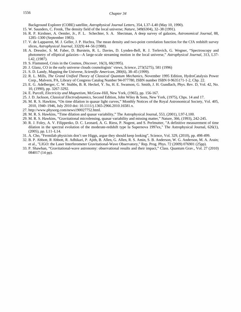
Chapter 34 1556
Background Explorer (COBE) satellite, Astrophysical Journal Letters, 354, L37–L40 (May 10, 1990). 15. W. Saunders, C. Frenk, The density field of the local universe; Nature, 349(6304), 32–38 (1991). 16. R. P. Kirshner, A. Oemler, Jr., P. L. Schechter, S. A. Shectman, A deep survey of galaxies, Astronomical Journal, 88,
1285–1300 (September 1983). 17. V. de Lapparent, M. J. Geller, J. P. Huchra, The mean density and two-point correlation function for the CfA redshift survey
slices, Astrophysical Journal, 332(9) 44–56 (1988). 18. A. Dressler, S. M. Faber, D. Burstein, R. L. Davies, D. Lynden-Bell, R. J. Terlevich, G. Wegner, “Spectroscopy and
photometry of elliptical galaxies—A large-scale streaming motion in the local universe,” Astrophysical Journal, 313, L37-L42, (1987).
19. S. Flamsteed, Crisis in the Cosmos, Discover, 16(3), 66(1995). 20. J. Glanz, CO in the early universe clouds cosmologists’ views, Science, 273(5275), 581 (1996) 21. S. D. Landy, Mapping the Universe, Scientific American, 280(6), 38–45 (1999). 22. R. L. Mills, The Grand Unified Theory of Classical Quantum Mechanics, November 1995 Edition, HydroCatalysis Power
Corp., Malvern, PA, Library of Congress Catalog Number 94-077780, ISBN number ISBN 0-9635171-1-2, Chp. 22. 23. E. G. Adelberger, C. W. Stubbs, B. R. Heckel, Y. Su, H. E. Swanson, G. Smith, J. H. Gundlach, Phys. Rev. D, Vol. 42, No.
10, (1990), pp. 3267-3292. 24. E. Purcell, Electricity and Magnetism, McGraw-Hill, New York, (1965), pp. 156-167. 25. J. D. Jackson, Classical Electrodynamics, Second Edition, John Wiley & Sons, New York, (1975), Chps. 14 and 17. 26. M. R. S. Hawkins, “On time dilation in quasar light curves,” Monthly Notices of the Royal Astronomical Society, Vol. 405,
2010, 1940–1946, July 2010 doi: 10.1111/j.1365-2966.2010.16581.x. 27. http://www.physorg.com/news190027752.html. 28. M. R. S. Hawkins, “Time dilation and quasar variability,” The Astrophysical Journal, 553, (2001), L97-L100. 29. M. R. S. Hawkins, “Gravitational microlensing, quasar variability and missing matter,” Nature, 366, (1993), 242-245. 30. R. J. Foley, A. V. Filippenko, D. C. Leonard, A. G. Riess, P. Nugent, and S. Perlmutter, "A definitive measurement of time
dilation in the spectral evolution of the moderate-redshift type Ia Supernova 1997ex," The Astrophysical Journal, 626(1), (2005), pp. L11–L14.
31. A. Cho, “Fermilab physicists don’t see Higgs, argue they should keep looking”, Science, Vol. 329, (2010), pp. 498-499. 32. B. P. Abbott, R Abbott, R. Adhikari, P. Ajith, B. Allen, G. Allen, R. S. Amin, S. B. Anderson, W. G. Anderson, M. A. Arain;
et al., "LIGO: the Laser Interferometer Gravitational-Wave Observatory," Rep. Prog. Phys. 72 (2009) 076901 (25pp). 33. P. Shawhan, “Gravitational-wave astronomy: observational results and their impact,” Class. Quantum Grav., Vol. 27 (2010)
084017 (14 pp).

1557
Chapter 35 THE FIFTH FORCE GENERAL CONSIDERATIONS The physical basis of the equivalence of inertial and gravitational mass of fundamental particles is given in the Equivalence of Inertial and Gravitational Masses Due to Absolute Space and Absolute Light Velocity section wherein spacetime is Riemannian due to a relativistic correction to spacetime with particle production. The Schwarzschild metric gives the relationship whereby matter causes relativistic corrections to spacetime that determines the curvature of spacetime and is the origin of gravity. Matter arises during particle production from a photon and comprises mass and charge confined to a two dimensional surface. Matter of fundamental particles such as an electron has zero thickness. But, in order that the speed of light is a constant maximum in any frame including that of the gravitational field that propagates out as a light-wave front at particle production, the production event gives rise to a spacetime dilation equal to 2 times the Newtonian gravitational or Schwarzschild radius
572
21.3525 10 e
g
Gmr X m
c of the particle according to Eqs. (32.36) and (32.140b) and the discussion at the footnote after
Eq. (32.40). For the electron, this corresponds to a spacetime dilation of 578.4980 10 X m or 652.8346 10 X s . Although the electron does not occupy space in the third spatial dimension, its mass discontinuity effectively “displaces” spacetime wherein the spacetime dilation can be considered a “thickness” associated with its gravitational field. Matter and the motion of matter effects the curvature of spacetime which in turn influences the motion of matter. Consider the angular motion of matter of a fundamental particle. The angular momentum of the photon is . An electron is formed from a photon, and it can only change its bound states in discrete quantized steps caused by a photon at each step. Thus, the electron angular momentum is always quantized in terms of . But this intrinsic motion comprises a two-dimensional current surface of the motion of the matter through space that may be positively curved, flat, or negatively curved. The first and second cases correspond to the bound and free electron, respectively. The third case corresponds to an extraordinary state of matter called a pseudoelectron given infra. Due to interplay between the motion of matter and spacetime in terms of their respective geometries, only in the first case are the inertial and gravitational masses of the electron equivalent. In the second case, the gravitational mass is zero. The experimental mass of the free electron measured by Witteborn [1] using a free fall technique is less than 0.09 em , where em is the inertial
mass of the free electron 319.109534 10 X kg consistent with the Classical Physics theoretical prediction. In the third case,
the gravitational mass is negative in the equations of extrinsic or translational motion. The negative gravitational mass of a fundamental particle is the basis of and is manifested as a fifth force that acts on the fundamental particle in the presence of a gravitating body in a direction opposite to that of the gravitational force with far greater magnitude1.
The two-dimensional nature of matter permits the unification of subatomic, atomic, and cosmological gravitation. The theory of gravitation that applies on all scales from quarks to cosmos as shown in the Gravity section is derived by first establishing a metric. A space in which the curvature tensor has the following form: , ( )R K g g g g (35.1)
is called a space of constant curvature; it is a four-dimensional generalization of Friedmann-Lobachevsky space. The constant
1 In the case of Einstein’s gravity equation (Eq. (32.40)), the Einstein Tensor G , is equal to the stress-energy-momentum tensor T . The only
possibility is for the gravitational mass to be equivalent to the inertial mass. A particle of zero or negative gravitational mass is not possible. However, it is shown in the Gravity section that the correct basis of gravitation is not according to Einstein’s equation Eq. (32.40); instead, the origin of gravity is the relativistic correction of spacetime itself which is analogous to the special relativistic corrections of inertial parameters—increase in mass, dilation in time, and contraction in length in the direction of constant relative motion of separate inertial frames. On this basis, the observed acceleration of the cosmos is predicted as given in the Cosmology section.

Chapter 35 1558
K is called the constant of curvature. The curvature of spacetime results from a discontinuity of matter having curvature confined to two spatial dimensions. This is the property of all matter at the fundamental-particle scale. Consider an isolated bound electron comprising an atomic orbital with a radius nr as given in the One-Electron Atom section. For radial distances, r ,
from its center with nr r , there is no mass; thus, spacetime is flat or Euclidean. The curvature tensor applies to all space of the
inertial frame considered; thus, for nr r , 0K . At nr r there exists a discontinuity of mass in constant motion within the
atomic orbital as a positively curved surface. This results in a discontinuity in the curvature tensor for radial distances nr . The
discontinuity requires relativistic corrections to spacetime itself. It requires radial length contraction and time dilation corresponding to the curvature of spacetime. The gravitational radius of the atomic orbital and infinitesimal temporal displacement corresponding to the contribution to the curvature in spacetime caused by the presence of the atomic orbital are derived in the Gravity section.
The Schwarzschild metric gives the relationship whereby matter causes relativistic corrections to spacetime that determines the curvature of spacetime and is the origin of gravity. The correction is based on the boundary conditions that no signal can travel faster than the speed of light including the gravitational field that propagates following particle production from a photon wherein the particle has a finite gravitational velocity given by Newton’s Law of Gravitation. The separation of proper time between two events x and x dx given by Eq. (32.38), the Schwarzschild metric [2-3], is:
1
2 2 2 2 2 2 2 20 02 2 2
2 211 1 sin
Gm Gmd dt dr r d r d
c r c c r
(35.2)
Eq. (35.2) can be reduced to Newton’s Law of Gravitation for gr , the gravitational radius of the particle, much less than *r , the
radius of the particle at production (*
1gr
r ), where the radius of the particle is its Compton wavelength bar ( *
cr ):
1 22
Gm mF
r (35.3)
where G is the Newtonian gravitational constant. Eq. (35.2) relativistically corrects Newton’s gravitational theory. In an analogous manner, Lorentz transformations correct Newton’s laws of mechanics.
The effects of gravity preclude the existence of inertial frames in a large region, and only local inertial frames, between which relationships are determined by gravity are possible. In short, the effects of gravity are only in the determination of the local inertial frames. The frames depend on gravity, and the frames describe the spacetime background of the motion of matter. Therefore, differing from other kinds of forces, gravity which influences the motion of matter by determining the properties of spacetime is itself described by the metric of spacetime. It was demonstrated in the Gravity section that gravity arises from the two spatial dimensional mass-density functions of the fundamental particles.
It is demonstrated in the One-Electron Atom section that a bound electron is a two-dimensional spherical shell—an
atomic orbital. On the atomic scale, the curvature, K, is given by 2
1
nr, where nr is the radius of the radial delta function of the
atomic orbital. The velocity of the electron is a constant on this two-dimensional sphere. It is this local, positive curvature of the electron that causes gravity due to the corresponding physical contraction of spacetime due to its presence as shown in the Gravity section. It is worth noting that all ordinary matter, comprised of leptons and quarks, has positive curvature. Euclidean plane geometry asserts that (in a plane) the sum of the angles of a triangle equals 180 . In fact, this is the definition of a flat surface. For a triangle on an atomic orbital the sum of the angles is greater than 180°, and the atomic orbital has positive curvature. For some surfaces the sum of the angles of a triangle is less than 180 ; these are said to have negative curvature.
sum of angles of triangles type of surface
> 180° positive curvature= 180° flat< 180° negative curvature
The measure of Gaussian curvature, K, at a point on a two-dimensional surface is:
1 2
1K
r r (35.4)
the inverse product of the radius of the maximum and minimum circles, 1r and 2r , which fit the surface at the point, and the radii
are normal to the surface at the point. By a theorem of Euler, these two circles lie in orthogonal planes. For a sphere, the radii of the two circles of curvature are the same at every point and are equivalent to the radius of a great circle of the sphere. Thus, the sphere is a surface of constant curvature;
2
1K
r (35.5)
at every point. In the case of positive curvature of which the sphere is an example, the circles fall on the same side of the surface, but when the circles are on opposite sides, the curve has negative curvature. A saddle, a cantenoid, a hyperboloid, and a

The Fifth Force
1559
pseudosphere are negatively curved. The general equation of a saddle is:
2 2
2 2
x yz
a b (35.6)
where a and b are constants. The curvature of the surface of Eq. (35.6) is:
22 2
2 2 4 4
1 1
4 4
x yK
a b a b
(35.7)
A saddle is shown schematically in Figure 35.1, a hyperboloid is shown in Figure 35.2, and a conic is shown in Figure 35.3. Figure 35.1. A saddle.
A pseudosphere is constructed by revolving the tractrix about its asymptote. For the tractrix, the length of any tangent measured from the point of tangency to the x-axis is equal to the height R of the curve from its asymptote—in this case the x-axis. The pseudosphere is a surface of constant negative curvature. The curvature, K
2
1 2
1 1K
r r R
(35.8)
given by the product of the two principal curvatures on opposite sides of the surface is equal to the inverse of R squared at every point where R is the equitangent. R is also known as the radius of the pseudosphere. A pseudosphere is shown schematically in Figure 35.4.
In the case of a sphere, surfaces of constant potential are concentric spherical shells. The general law of potential for
Figure 35.3. A conic.
Figure 35.2. A hyperboloid.
Figure 35.4. A pseudosphere.

Chapter 35 1560
surfaces of constant curvature is:
0 1 2 0
1 1 1
4 4V
r r R (35.9)
In the case of a pseudosphere the radii 1r and 2r , the two principal curvatures, represent the distances measured along the normal
from the negative potential surface to the two sheets of its evolute, envelop of normals (cantenoid and x-axis). The force is
given as the gradient of the potential that is proportional to 2
1
r in the case of a sphere.
All matter is comprised of fundamental particles, and all fundamental particles exist as mass confined to two spatial dimensions. The particle’s current surface is positively curved in the case of an atomic orbital, flat in the case of a free electron, and negatively curved in the case of an electron as a pseudosphere hereafter called a pseudoelectron. The effect of this “local” curvature on the non-local spacetime is to cause it to be Riemannian in the case of an atomic orbital, or hyperbolic, in the case of a pseudoelectron, as opposed to Euclidean in the case of the free electron. Each curvature is manifest as a gravitational field, a repulsive gravitational field, or the absence of a gravitational field, respectively. Thus, the spacetime is curved with constant spherical curvature in the case of an atomic orbital, or spacetime is curved with negative curvature in the case of a pseudoelectron.
Matter arises during particle production from a photon. The limiting velocity c results in the contraction of spacetime due to particle production. The contraction is given by 2 gr where gr is the gravitational radius of the particle. This has
implications for the physics of gravitation. By applying the condition to electromagnetic and gravitational fields at particle production, the Schwarzschild metric (SM) is derived from the classical wave equation, which modifies general relativity to include conservation of spacetime in addition to momentum and matter/energy. The result gives a natural relationship between Maxwell’s equations, special relativity, and general relativity. It gives gravitation from the atom to the cosmos. The Schwarzschild metric gives the relationship whereby matter causes relativistic corrections to spacetime that determines the curvature of spacetime and is the origin of gravity. The gravitational equations with the equivalence of the particle production energies permit the equivalence of mass-energy and the spacetime wherein a “clock” is defined which measures “clicks” on an observable in one aspect, and in another, it is the ruler of spacetime of the Universe with the implicit dependence of spacetime on matter-energy conversion. The masses of the leptons, the quarks, and nucleons are derived from this metric of spacetime.
The relativistic correction for spacetime dilation and contraction due to the production of a particle with positive curvature is given by Eq. (32.17):
2
1 gvf r
c
(35.10)
As shown in the Gravity section (Eq. (32.35)), the derivation of the relativistic correction factor of spacetime was based on the constant maximum velocity of light and a finite positive Newtonian gravitational velocity gv of the particle. The production of a
particle requires that the velocity of the particle is equivalent to the Newtonian gravitational escape velocity, gv , of the
antiparticle:
0 02 2g
C
Gm Gmv
r
(35.11)
From Eq. (35.22) and Eqs. (35.18-35.19), the eccentricity is one and the particle production trajectory is a parabola relative to the center of mass of the antiparticle. The right-hand side of Eq. (32.43) represents the correction to the laboratory coordinate metric for time corresponding to the relativistic correction of spacetime by the particle production event. Consider a Newtonian gravitational radius, gr , of each atomic orbital of the particle production event, each of mass 0m
02
2g
Gmr
c (35.12)
where G is the Newtonian gravitational constant. The substitution of each of Eq. (35.11) and Eq. (35.12) into the Schwarzschild metric Eq. (35.2) gives:
12 2
2 2 2 2 2 2 2 22
11 1 sing gv v
d dt dr r d r dc c c
(35.13)
and

The Fifth Force
1561
1
2 2 2 2 2 2 2 22
11 1 sing gr r
d dt dr r d r dr c r
(35.14)
respectively. The solutions for the Schwarzschild metric exist wherein the relativistic correction to the gravitational velocity gv
and the gravitational radius gr are of the opposite sign (i.e. negative). In these cases, the Schwarzschild metric (Eq. (35.2)) is:
12 2
2 2 2 2 2 2 2 22
11 1 sing gv v
d dt dr r d r dc c c
(35.15)
and
1
2 2 2 2 2 2 2 22
11 1 sing gr r
d dt dr r d r dr c r
(35.16)
The metric given by Eqs. (35.13-35.14) corresponds to positive curvature. The metric given by Eqs. (35.15-35.16) corresponds to negative curvature. The positive curvature of spacetime arises from the conversion of a photon traveling at light speed and having no gravitational mass into a bound particle-antiparticle pair such as an electron-positron pair each having its inertial rest mass relative to the corresponding particle’s absolute space (Equivalence of Inertial and Gravitational Masses Due to Absolute Space and Absolute Light Velocity section). The escape velocity is the gravitational velocity gv following a parabolic orbit with
both particles traveling to an unbound state with relative velocity with respect to the absolute space corresponding to the excess energy over the mass energy of the particles (Gravity section). Both free particles such as leptons and antileptons exist with zero curvature. Each zero-curvature particle is predicted to have a zero gravitational mass and a zero gravitational radius based on continuity of the spacetime metric relationships given by Eqs. (35.13-35.14).
The equations that govern the production and trajectories of fundamental particles (Quantum Gravity of Fundamental Particles section and Particle Production section) also apply to the mechanical equations of existing particles. Bound and free electrons are natural states for inverse-r potentials. Yet, a third extraordinary state is possible for the correspondence between the geometrical form of the mass and the intrinsic motion of particles and their effect on spacetime which in turn affects the extrinsic motion of the particles. Specifically, the particle may possess a negative gravitation radius and a corresponding imaginary velocity. The metric given by Eqs. (35.13-35.14) corresponds to positive curvature; whereas, the metric given by Eqs. (35.15-35.16) corresponds to the extraordinary case of negative curvature. Spacetime having positive curvature in turn affects the extrinsic motion of the negatively curved particle such as a one having mass and intrinsic motion confined to a negatively curved two-dimensional membrane in the form of a pseudosphere, pseudoelectron, to give rise to an imaginary translational velocity corresponding to a hyperbolic orbit along the gradient of the positive curvature. Thus, negative gravity (fifth force) can be created by forcing matter into negative curvature. A fundamental particle such as an electron with negative curvature, pseudoelectron, would experience a central but repulsive force with a gravitating body comprised of matter of positive curvature. In this case, the fifth force deflects the pseudoelectron upward such that the negatively curved electron has the translational kinetic energy that causes the coordinate and proper times to be equivalent according to the Schwarzschild metric. Masses and their effects on spacetime superimpose; thus, the metric corresponding to the Earth is given by substitution of the mass of the Earth, M , for 0m in Eqs. (35.11-35.16). The corresponding Schwarzschild metric Eq. (35.2) is:
1
2 2 2 2 2 2 2 22 2 2
2 1 21 1 sin
GM GMd dt dr r d r d
c r c c r
(35.17)
which is the gravitational mechanics equation that can be expressed in terms of the gravitational velocity gv and the gravitational
radius gr as given by Eqs. (35.13-35.16) with the mass being that of the Earth 245.98 10 M X kg .
POSITIVE, ZERO, AND NEGATIVE GRAVITATIONAL MASS The geometry of an electron’s 2-dimensional mass surface determines that the electron may have a gravitational mass different from its inertial mass. A bound electron comprising a positively curved mass with its intrinsic surface velocity corresponds to a positive gravitational mass equal to the inertial mass (e.g. particle production or a bound electron). An absolutely free electron comprising a flat surface corresponds to zero gravitational mass with inertial mass em . A pseudoelectron comprising negatively
curved mass with its intrinsic surface velocity corresponds to a negative gravitational mass with inertial mass em . Each case is
considered in turn infra. According to Newton’s Law of Gravitation, the production of a particle of finite mass gives rise to a gravitational
velocity of the particle that is essential in the determination of the particle masses as given in the Quantum Gravity of Fundamental Particles section and Particle Production section. The gravitational velocity of a gravitating body such as the Earth, the velocity of an existing particle, and the nature of its gravitational mass determines the energy, eccentricity, and trajectory of

Chapter 35 1562
the gravitational orbit of the particle. Consider the case of the equivalence of inertial and gravitational masses. The eccentricity, e, given by Newton’s differential equations of motion in the case of the central field (Eq. (32.49-32.50)) permits the classification of the orbits according to the total energy, E, and according to the orbital velocity, 0v , relative to the Newtonian
gravitational escape velocity, gv , as follows [4]. The same relationships hold for trajectories during particle production and
motion of existing particles: 0 1E e ellipse 0 0E e circle (special case of ellipse) (35.18) 0 1E e parabolic orbit 0 1E e hyperbolic orbit
2 20
0
21g
GMv v e
r ellipse
2 20
0
20g
GMv v e
r circle (special case of ellipse)
2 20
0
21g
GMv v e
r parabolic orbit (35.19)
2 20
0
21g
GMv v e
r hyperbolic orbit
Since E T V and is constant, the closed orbits are those for which | |T V , and the open orbits are those for which | |T V . It can be shown that the time average of the kinetic energy, T , for elliptic motion in an inverse square field is 1/ 2 that of the time average of the potential energy, V : 1/ 2T V .
In the case that a particle of inertial mass, m , is observed to have a speed, 0v , a distance from a massive object, 0r , and a
direction of motion makes that an angle, , with the radius vector from the object (including a particle) of mass, M, the total energy is given by:
2 20
0
1 1constant
2 2
GMm GMmE mv mv
r r (35.20)
The orbit will be elliptic, parabolic, or hyperbolic, according to whether E is negative, zero, or positive. Accordingly, if 2
0v is
less than, equal to, or greater than 0
2GM
r, the orbit will be an ellipse, a parabola, or a hyperbola, respectively. Since h, the
angular momentum per unit mass, is: 0 0/ sinh L m r v r v (35.21)
the eccentricity, e, from Eq. (32.63) may be written as:
2 2 2
2 1/20 00 2 2
0
sin2[1 ]
r vGMe v
r G M
(35.22)
The nature of the sign of the parameters 2gv and gr (Eqs. (35.13-35.16)) with the corresponding mechanics equations determine
the behavior of the electron of a given curvature in terms of the classification of the gravitational mass being positive, zero, or negative in the historical Newtonian or general relativistic view. In the last two cases, the inertial and gravitational masses are not equivalent. Consider the first case. The particle production equation (Eq. (32.43)) is for isolated particles at infinity wherein the gravitational and inertial masses are equal. A discontinuity in mass in positive curvature gives rise to a discontinuity in the positive curvature of spacetime that is the origin of gravity. Even at infinity relative to each other, each member of a production pair of particles is still in positive curvature due to the charge neutrality condition that requires that the field lines of one particle terminate on the other. The central field exists and maintains a positive curvature that maintains the equivalence of inertial and gravitational masses. The electric and magnetic fields of a particle are considered part of its inertial mass. This inertial mass is released as photons corresponding to the binding energy BE of the oppositely charged particle. So, the sum of the masses of
bound particles is less by 2BE
c. The gravitational mass also decreases by this amount since the released photons have no
gravitational mass as given in the Deflection of Light section. In a special case, a free electron can be maintained in the essential

The Fifth Force
1563
absence of fields and without spin angular momentum by cancellation with orbital angular momentum such that the curvature is no longer positive, and the inertial and gravitational masses are no longer equivalent.
Minkowski space applies to the free electron. In the Electron in Free Space section, a free electron is shown to be a two-dimensional plane wave—a flat surface. Because the gravitational mass depends on the positive curvature of a particle, a free electron has inertial mass but not gravitational mass. If the electric and magnetic fields are essentially eliminated from a region of vacuum space containing an electron such that the electron is completely free and unbound and the spin angular momentum is cancelled, it may be possible to measure an electron gravitational mass that is less than the inertial mass em . The gravitational
mass is zero in the limit of the electron being absolutely free. With the exclusion of electromagnetic fields and the cancelation of the spin angular momentum, Witteborn [1] experimentally measured the gravitational mass of the free electron using a free fall technique. The reported result was less than 0.09 em , where em is the inertial mass of the free electron 319.109534 10 X kg .
Thus, a free electron is not gravitationally attracted to ordinary matter, and the gravitational and inertial masses are not equivalent. Witteborn [1] explains the observation that free electrons floated in the drift tube by a postulated Schiff—Barnhill effect wherein the electrons in the metal of the drift tube fall in the Earth’s gravitational field to produce an electric field which identically balances the force of gravity on the free electrons in the drift tube. This explanation is untenable. The binding energy of electrons in metals is typically 5 eV; whereas, the gravitational potential energy over atomic dimensions is over 20 orders of magnitude less and is given by eE m gh where em is the mass of the electron, g is the acceleration of gravity, and h is
the metal internuclear spacing, about 1010 m . The positive nuclei weigh 4,000 times the mass of the electrons. And, this zero mass equivalent electrical force requires the achievement of a perfect Penning trap having 11 orders of magnitude strength match at six-figure accuracy using gravity as the source of trapping field by pure chance!
The reluctance to accept the experimental results of the free electron gravitational mass is that it would violate the Equivalence Principle and disprove general relativity2. This bias is evident in the presentation of the findings of the 2nd International Workshop on Antimatter and Gravity that took place on November 13–15, 2013 at the Albert Einstein Center for Fundamental Physics of the University of Bern. One of the main topics was on the results of the measurement of the gravitational mass of the free electron. The CERN Courier [5] reports:
“Free-fall experiments with charged particles are notoriously difficult because they must be carefully shielded from
electromagnetic fields. For example, the sagging of the gas of free electrons in metallic shielding induces an electric field that can counterbalance the effect of gravity. Indeed, measurements based on dropping electrons led to a value of the acceleration of gravity, g, consistent with zero (instead of g = 9.8 m/s2).”
Indeed the predicted gravitational mass of the free electron is zero.
Another reservation against the acceptance of the measurement of the zero gravitational mass of the free electron is that under the equivalence principle a perpetual motion scheme could be devised: (1) the free electron is formed with the application of a 13.6 eV photon to a hydrogen atom, (2) the proton and free electron are transported to infinity relative to the Earth, (3) the free electron binds with the proton to return the 13.6 eV photon, (4) the atom comprising a bound electron having a gravitational mass equivalent to the inertial mass falls to the Earth to net produce “free energy” from the added gravitational energy with the free electron now bound becoming gravitationally massive on the return trip. This scenario is an infinitely repeatable cycle; thus, it comprises perpetual motion. The reason why this is not the case is that it requires exactly the gravitation potential energy of the electron’s inertial mass to exclude all fields, cancel spin, and form an absolutely free electron. The gravitational energy to completely eliminate any electric field termination on its surface and cancel the spin angular momentum such at it is absolutely free is given by:
11 2 2 31 24
6
23 4
6.67 10 / 9.11 10 5.98 10
6.37 10
5.70 10 3.56 10
G
X N m kg X kg X kgGMmV
r X m
X J X eV
(35.23)
wherein 66.37 10 r X m is the radius of the Earth. Furthermore, it is possible to give the electron negative curvature to cause a fifth force with negative gravitational mass
behavior. Hereto, energy must be applied to form this state so no perpetual motion scheme is possible. The negative mass behavior can be modeled as a hyperbolic trajectory of a pseudoelectron. A particle comprising a gravitating body is the source of local spacetime curvature that is negative in the case of a pseudoelectron. In the presence of the large positive curvature of the Earth, the corresponding gravitational velocity is imaginary, the energy of the orbit of the pseudoelectron must always be greater than zero, the eccentricity is always greater than one, and the trajectory is a hyperbola (Eqs. (35.18-35.19) and (35.22)). The gravitational mass of the pseudoelectron behaves as negative and the inertial mass em is constant (e.g. equivalent to its mass
energy given by Eq. (33.13)). The trajectory of pseudoelectrons can be found by solving the Newtonian inverse-square gravitational force equations for the case of a repulsive force caused by pseudoelectron production. The trajectory follows from the Newtonian gravitational force and the solution of motion in an inverse-square repulsive field is given by Fowles [6]. The
2 The original Equivalence Principle put forth by Einstein was the equivalence of an accelerating inertial frame and a gravitational field that was shown to be incorrect and modified by others.

Chapter 35 1564
trajectory can be calculated rigorously by solving the orbital equation from the Schwarzschild metric (Eqs. (35.15-35.16)) for a two-dimensional spatial mass-density function of negative curvature which is repelled by the Earth. The rigorous solution is equivalent to that given for the case of a positive gravitational velocity given in the Orbital Mechanics section except that the gravitational velocity is imaginary and the magnitude is determined by the negative curvature.
In the case of a mass of negative curvature, Eq. (32.77) becomes
g
GMmE
r (35.24)
where M is the mass of the Earth and m is the gravitational mass of the pseudoelectron that is negative, different from its inertial mass, and depends on the negative curvature. The negative curvature is determined by the Gaussian curvature, K, at a point on a two-dimensional surface given by Eqs. (35.4-35.5) and (35.8). According to Eqs. (32.48), (32.140) and (32.43), matter, energy, and spacetime are conserved with respect to creation of the pseudoelectron which is repelled from a gravitating body (e.g. the Earth). The ejection of a pseudoelectron having a negatively curved mass surface from the Earth must result in an infinitesimal decrease in the radius of the Earth (e.g. r of the Schwarzschild metric given by Eq. (35.2) where 0m M is the
mass of the Earth, 245.98 10 X kg ). The amount that the gravitational potential energy of the Earth is lowered is equivalent to the total energy gained by the repelled pseudoelectron. As an offsetting contribution to the curvature inventory, the conversion of matter to energy to produce the photon that excites the pseudoelectron state causes spacetime expansion according to Eq. (32.140). Upon decay, the energy is available to be absorbed to increase the equivalent inertial and gravitational masses of matter in positive curvature. Momentum is also conserved for the pseudoelectron and Earth, wherein the latter gravitating body that repels the pseudoelectron, receives an equal and opposite change of momentum with respect to that of the electron. As a familiar example, causing a satellite to follow a hyperbolic trajectory about a gravitating body is a common technique to achieve a gravity assist to further propel the satellite. In this case, the energy and momentum gained by the satellite are also equal and opposite those lost by the gravitating body. Next, the mathematical structure, nature, and energies of the pseudoelectron will be elucidated.
DETERMINATION OF THE PROPERTIES OF ELECTRONS, THOSE OF CONSTANT NEGATIVE CURVATURE, AND THOSE OF PSEUDOELECTRONS
The candidates for a negatively curved electron state are shown in Figures 35.1-35.4. By rotating a curve in the xz-plane about the z-axis, an exemplary surface of revolution with constant Gaussian curvature having 1K is generated. Consider that the Cartesian coordinate curve profile is given by:
,0,c t x t z t (35.25)
parameterized by arc length
2 21x t z t (35.26)
The Gaussian curvature of the corresponding surface of revolution
, cos , sin ,f u v x u v x u v z u (35.27)
is then given by
, 1x u
K u vx u
(35.28)
Since 1K is a constant, Eq. (35.28) gives rise to the second-order differential equation:
0x t x t (35.29)
that is solved analytically to give:
t tx t ae be (35.30)
where a and b are constants to match boundary conditions. The corresponding function z is then calculated from Eq. (35.26) by numerical integration to give the surface shown in Figure 35.5 [7]. Alternatively, the analytical expressions are given by M. Spivak [8] for the case of a b :
2 sinht tx t a e e a t (35.31)
2 2
0
( ) 1 4 cosht
z t a tdt (35.32)

The Fifth Force
1565
wherein 0 2 1a and 1 cosh 1/ 2t a , so that 10 cosh 1/ 2a and 20 ( ) 1 4g t a . These are functions that can be expressed in terms of elliptic integrals with results shown in Figure 35.5.
A free electron avoids a singularity by having the current density approaching zero at the extrema. A nonphysical aspect of the candidate shown in Figure 35.5 having a negatively curved surface are the singularities at the extrema. In contrast, the pseudosphere (Figure 35.6) generated by rotating the tractrix about the asymptote avoids such a singularity and maintains current continuity at infinity. The mass goes to zero at the extrema at infinity since the corresponding area goes to zero, the current has an increasing azimuthal component at the extrema at infinity to maintain continuity, and relativistic effects cause the asymptotic span to be finite. Moreover, the constant radius R of the pseudosphere is permissive of a central force balance that is stable to radiation and conserves the electron angular momentum of as shown in the Fourier Transform of the Pseudoelectron Current Density section and the Force Balance and Electrical Energies of Pseudoelectron States section. The nature of a pseudoelectron comprising an autonomous electron with a bound photon to maintain its surface of constant negative curvature can be appreciated by comparing it to other photon-electron states and the nature of the unnormalized atomic orbital current density distribution shown in Figure 1.20 and the normalized one shown in Figure 1.21.
NATURE OF PHOTONIC SUPER BOUND HYDROGEN STATES AND THE CORRESPONDING CONTINUUM EXTREME ULTRAVIOLET (EUV) TRANSITION EMISSION AND SUPER FAST ATOMIC HYDROGEN
J. R. Rydberg showed that all of the spectral lines of atomic hydrogen were given by a completely empirical relationship:
2 2
1 1
f i
Rn n
(35.33)
where 1109,677 , 1, 2,3,..., 2,3, 4,...f iR cm n n and i fn n . Bohr, Schrödinger, and Heisenberg, each developed a theory
for atomic hydrogen that gave the energy levels in agreement with Rydberg's equation:
2
2 2
13.598
8no H
e eVE
n a n (35.34)
1, 2,3,...n (35.35)
where e is the elementary charge, o is the permittivity of vacuum, and Ha is the radius of the hydrogen atom. The Rydberg
equation is a simple integer formula that empirically represents the Rydberg series of spectral lines, the entire hydrogen spectrum given in terms of the differences between all of the principal energy levels of the hydrogen atom.
The excited energy states of atomic hydrogen are given by Eq. (35.35) for 1n in Eq. (35.34). The 1n state is the "ground" state for "pure" photon transitions (i.e. the 1n state can absorb a photon and go to an excited electronic state, but it cannot release a photon and go to a lower-energy electronic state). However, an electron transition from the ground state to a lower-energy state may be possible by a resonant nonradiative energy transfer such as multipole coupling or a resonant collision mechanism. Processes such as hydrogen molecular bond formation that occur without photons and that require collisions are common [9]. Also, some commercial phosphors are based on resonant nonradiative energy transfer involving multipole coupling [10]. Specifically, atomic hydrogen may undergo a catalytic reaction with certain atomized elements and ions which
Figure 35.5. The half-space surface rendering of a constant Gaussian curvature 1K . The complete surface comprises additionally the mirror image.
Figure 35.6. A pseudosphere showing rulings of the tractrix along the asymptote axis.

Chapter 35 1566
singly or multiply ionize at integer multiples of the potential energy of atomic hydrogen, 27.2 m eV wherein m is an integer. The predicted reaction involves a resonant, nonradiative energy transfer from otherwise stable atomic hydrogen to the catalyst capable of accepting the energy. The product is 1/H p , fractional Rydberg states of atomic hydrogen called "hydrino atoms"
wherein 1 1 1 1
, , ,...,2 3 4
np
( 137p is an integer) replaces the well-known parameter integern in the Rydberg equation for
hydrogen excited states.
The 1n state of hydrogen and the 1
integern states of hydrogen are nonradiative, but a transition between two
nonradiative states, say 1n to 1/ 2n , is possible via a nonradiative energy transfer. Hydrogen is a special case of the stable states given by Eqs. (35.34) wherein the corresponding radius of the hydrogen or hydrino atom is given by:
Har
p , (35.36)
where 1, 2,3,...p . In order to conserve energy, energy must be transferred from the hydrogen atom to the catalyst in units of 27.2 m eV , 1, 2,3, 4,....m (35.37)
and the radius transitions to Ha
m p. The catalyst reactions involve two steps of energy release: a nonradiative energy transfer to
the catalyst followed by additional energy release as the radius decreases to the corresponding stable final state. Thus, the general reaction is given by:
27.2 * 27.2 ( )
q rq H Hfast
a am eV Cat H Cat re H m eV
p m p
(35.38)
2 2* [( ) ] 13.6 27.2 ( ) ( )
H Ha aH H p m p eV m eV
m p m p
(35.39)
27.2 q r qfastCat re Cat m eV (35.40)
And, the overall reaction is:
2 2[( ) ] 13.6 ( )
H Ha aH H p m p eV
p m p
(35.41)
q , r , m , and p are integers.
* HaH
m p
has the radius of the hydrogen atom (corresponding to 1 in the denominator) and a
central field equivalent to m p times that of a proton, and
HaH
m p
is the corresponding stable state with the radius of
1
m p that of H . As the electron undergoes radial acceleration from the radius of the hydrogen atom to a radius of
1
m p
this distance, energy is released as characteristic light emission or as third-body kinetic energy. The emission may be in the form
of an extreme-ultraviolet continuum radiation having an edge at 2 2[( ) 2 ] 13.6 p m p m eV or 2 2
91.2
[( ) 2 ]nm
p m p m and
extending to longer wavelengths [11-17]. In addition to radiation, a resonant kinetic energy transfer from
* HaH
m p
to form
fast H may occur by an inverse Franck-Hertz mechanism [18] involving H atoms rather than electrons that are selective for H based on resonant dipole induction and H being the most efficient momentum acceptor having the least mass of any atom (See the Dipole-Dipole Coupling section). Subsequent excitation of these fast 1H n atoms by collisions with the background
gases followed by emission of the corresponding 3H n atoms gives rise to broadened Balmer emission. Fast H may also
arise from the production of fast protons that conserve the potential energy of the catalyst that is ionized during the energy transfer wherein the catalyst comprises a source of H such as HOH or nH ( n is an integer) catalyst. The fast protons recombine with electrons to give the characteristic Doppler broadened atomic H lines such as broadened Balmer alpha emission observed experimentally [19-25].
Visible photons and extremely high-energy photons, respectively, may excite the formation of photon bound, autonomous electron states such as spherical states in liquid media and inverse spherical states in vacuum or gas. The former case regards the formation of photon bonding of an atomic orbital current density function as given in the One Electron Atom section. In the latter case, a free electron is in a nonradiative bound state comprising geometry that is the inverse of a bound excited state. Specifically, a free electron may form an inverse spherical bound state of pseudospherical mass, charge, and surface current density bound by a trapped photon that travels along the two-dimensional electron surface as in the case of the

The Fifth Force
1567
excited states, but the photon field is repulsive rather than attractive, such that the direction of the centrifugal forces is also opposite the spherical case. Here, the energy to form the stable bound state is not due to a negative electrostatic potential. Rather, the binding energy is due to the negative gravitational potential energy that arises from the mass, charge, and current density surface in negative curvature. The pseudospherical electron state is referred to as a pseudoelectron. The formation of a pseudoelectron requires the presence of a gravitating body wherein the gravitational energy is conserved between the gravitating body and the pseudoelectron. Specifically, the positive curvature of spacetime due to the gravitating body is increased causing a more negative gravitational energy in response to the negative curvature contribution of the pseudoelectron that consequently experiences a force to eject it from the spacetime in proximity to the gravitating body. The change in positive curvature and corresponding gravitational field propagate as a light-like wave as in the case with particle production given in the Quantum Gravity of Fundamental Particles section.
NATURE OF PHOTON-BOUND AUTONOMOUS ELECTRON STATES As shown in the Free Electrons in Superfluid Helium are Real in the Absence of Measurement Requiring a Connection of
Ψ(x) to Physical Reality section, free electrons are trapped in superfluid helium as autonomous electron bubbles interloped between helium atoms that have been excluded from the space occupied by the bubble [26-29]. The surrounding helium atoms maintain the spherical bubble through van der Waals forces. Each spherical electron cavity comprises an atomic orbital that can act as a resonator cavity. The excitation of the Maxwellian resonator cavity modes by resonant photons forms bubbles with radii of reciprocal integer multiples of that of the unexcited n 1 state. The central force that results in a fractional electron radius compared to the unexcited electron is provided by the absorbed photon. Each stable excited state electron bubble that has a
radius of 1
integer
r may migrate in an applied electric field. The photo-conductivity absorption spectrum of free electrons in
superfluid helium and their mobilities predicted from the corresponding size and multipolarity of these long-lived bubble-like states with quantum numbers n , ℓ, and m
ℓ matched the experimental results of the 15 identified ions [26].
In addition to superfluid helium, free electrons also form bubbles devoid of any atoms in other fluids such as oils and liquid ammonia. In the operation of an electrostatic atomizing device, Kelly [30] observed that with plasma light irradiation the mobility of free electrons in oil increased by an integer factor rather than continuously. Certain metals such as alkali metals that have low ionization energy dissolve as ions and free electrons in liquid ammonia and certain other solvents. As in the case of free electrons in superfluid helium, ammoniated free electrons form cavities devoid of ammonia molecules having a typical diameter of 3-3.4 Å. The cavities are evidenced by the observation that the solutions are of much lower density than the pure solvent. From another perspective, they occupy far too great a volume than that predicted from the sum of the volumes of the metal and solvent. The electrolytically conductive solutions have free electrons of extraordinary mobility as their main charge carriers [31]. In very pure liquid ammonia the lifetime of free electrons can be significant with less than 1% decomposition per day. The confirmation of their existence as free entities is given by their broad absorption around 15,000 Å that can only be assigned to free electrons in the solution that is blue due to the absorption. In addition, magnetic and electron spin resonance studies show the presence of free electrons, and a decrease in paramagnetism with increasing concentration is consistent with spin pairing of electrons to form diamagnetic pairs.
In the case of vacuum, there is no solvent sphere; consequently, new physics may be observed with high energy irradiation of electrons, namely the formation of pseudoelectrons each comprising a pseudospherical charge and current density membrane held in force balance by a trapped photon. In the case of free electrons in a liquid medium such as superfluid helium, ammonia, or oil, the geometry is driven by minimization of the surface to volume ratio similar to the case with surface tension of bubble films. In contrast, the formation of a pseudoelectron depends on maximizing the negative gravitational potential energy that also results in the further minor energy contribution to stability of the minimization of the electric self-field energy. This occurs by maximizing the surface to volume ratio to diffuse the electric field. By both mechanisms, the energy stability is achieved by minimizing the pseudosphere volume (Eq. (35.100)) that also maximizes the curvature K of pseudoelectron having a 2R dependency where R is the pseudoelectron radius (Eq. (35.8)). In addition, the nature of the absorbed photon of the particular electronic state determines its stability or instability wherein the nature of the absorbed photon is dependent on the geometry or curvature of the electron comprising a 2-D current membrane, any nuclear field, and the energy of the state.
As shown by Eqs. (35.38-35.41), the photonic contribution to the central field of a hydrino is positive. Specifically, at the position of the electron, the photon field provides the equivalent of a positive integer increase to the central field of the proton (Eq. (5.27)) that gives rise to a radial monopole (Eq. (6.9)). Conversely, at the position of the electron, the excited state photon field comprises the superposition of two components, the negative equivalent of the central field of the proton and a positive reciprocal integer times the equivalent of the central field of the proton (Eqs. (2.12-2.17)). The opposing components give rise to the sum of a radial dipole (Eq. (2.25))) and a positive spherical and time harmonic monopole having the field equivalents of the fundamental charge and a fraction of the fundamental charge, respectively. The photonic central field of the pseudoelectron is purely negative; thus, the photon field gives rise to a corresponding pure radial monopole at the position of the electron. The stability of the pseudoelectron (Eqs. (35.72)) versus the instability of an electronic excited state (Eqs. (2.29-2.35)) arises from the different states having negative curvature versus positive curvature, respectively. The different geometries cause the corresponding current densities to be absent and possess Fourier components synchronous with waves traveling at the speed

Chapter 35 1568
of light, respectively, that determine stability to radiation as given in the Fourier Transform of the Pseudosphere Current Density section.
The radiative states comprise the hydrino intermediate (atomic hydrogen following energy transfer to a catalyst), excited states, and free electron states undergoing acceleration wherein the mechanism of charge acceleration may be generalized to all three cases. The nonradiative cases are hydrogen ( 1n state), hydrino states, spherical states in a liquid medium, these states with an absorbed photon, and free electrons at rest or constant velocity. The lifetime of the pseudoelectron state may be long as it is in the case of the continuum excited states of free electrons comprising a bound photon and negative gravitational potential energy to maintain the state with kinetic energy equal to ½ the excitation energy as shown in the Classical Physics of the de Broglie Relation section.
PSEUDOELECTRONS Surfaces shown in Figures 35.1-35.4 are candidates for a negatively curved electron state to produce the sought negative
gravitational force according to Eqs. (35.15-35.16). The boundary constraints are a surface of constant negative Gaussian curvature and capable of binding a photon and maintaining mechanical and electrical force balance with the relativistic photon field normal to the electron surface as given in the Equation of the Electric Field inside the Atomic Orbital section, relativistic invariance and total energy conservation of the equation of motion on the surface, and stability of the current to radiation. Let’s first solve the equivalent of the great circle current loop of the Atomic Orbital Equation of Motion for = 0 Based on the Current Vector Field (CVF) section in hyperbolic coordinates. By rotating a curve in the xz-plane about the z-axis, an exemplary surface of revolution with constant Gaussian curvature having 1K is generated. Consider that the alternative Cartesian coordinate curve profile given by Eqs. (35.25-35.30) for the case of 1a and 0b . Eq. (35.30) becomes:
tx t ae (35.42)
Using Eq. (35.26), Eq. (35.32) becomes:
2 2 1
0
1 1 cosht
t t tz t e dt e e (35.43)
replacing some variables gives the xz-cross section of a pseudosphere shown in Figure 35.6 having the equation:
2 1 11 coshz x
x (35.44)
A pseudosphere also called a tractroid, tractricoid, antisphere, or tractrisoid comprises a negative-Gaussian curvature surface 1K of revolution generated by a tractrix in the xy-plane about its asymptote, the z-axis. The pseudosphere of radius
0r is the image R [0, 2 [R having Cartesian parametric equations of:
2
sech cos
, sech sin
tanh
r u v
u v r u v
ru r u
r e (35.45)
for u , and v[0,2 ) . Alternatively, the pseudosphere can be expressed in Cartesian form as:
22 2
2 1 2 2 2sechx y
z R R x yR
(35.46)
A pseudoelectron shown in Figures 35.6 and 35.7 comprises a pseudospherical plane lamina of charge and current density comprising a minimum total energy surface having constant negative curvature of 1K . The pseudospherical membrane is bound by a photon. The absorbed photon of the pseudoelectron provides a repulsive central electric field that maintains the pseudoelectron in force balance between the centrifugal and corresponding electrostatic force wherein the directions of the centrifugal and electrostatic forces relative to the direction along the central radius are opposite those of hydrino and excited states, and negative binding energy is from the negative gravitational potential energy of the state of constant negative curvature.

The Fifth Force
1569
Figure 35.7. A representation of a pseudoelectron.
The pseudosphere is a solution of the sine-Gordon equation. Consider that the pseudosphere may be described as a map ,x u v
from a patch to the surface. If the map is parametrized by arclength along asymptotic lines, then the first fundamental
form for the pseudosphere is:
2 22cosdx dx du dudv dv I
(35.47)
Similarly, the second fundamental form is:
2
sindx dN dudv
II
(35.48)
Application of the Codazzi-Mainardi equations then yields [32]
2
1sinuv
(35.49)
which is the sine-Gordon equation that can be written as:
2 2
2 2sin 0
t x
(35.50)
The sine-Gordon equation also meets the prerequisite of being invariant under Lorentz transforms. The relevant Lorentz transforms are:
2
'vx
t tc
(35.51)
'x x vt (35.52)
'y y (35.53)
'z z (35.54)
wherein the inverse Lorentz transformations are given by interchanging the primed and unprimed variables and changing the sign of the velocity. The spacetime sine-Gordon equation (Eq. (35.50)) can be expressed in spacetime coordinates as:
sin 0tt xx (35.55)
Using the consideration that is a constant, Eq. (35.55) can be expressed in the primed coordinates using the following relationships of the time-coordinate:

Chapter 35 1570
' 't t t
dt
dt (35.56)
2' ' ' 't t t tt ttt t
(35.57)
The corresponding space-coordinate relationship is:
2' 'x x xx (35.58)
Using Eqs. (35.55-35.58), the transformed sine-Gordon equation is:
' ' ' ' 2
1sin 0t t x x
(35.59)
The equations of motion of matter and energy that are a solution of the sine-Gordon equation obey the laws of the universe wherein higher velocity gives rise to relativistic length contraction and mass increase of the electron mass density function as given in the Special Relativistic Effect on the Electron Radius and the Relativistic Ionization Energies section.
The sine-Gordon equation can be derived from the Lagrangian with the proper setting of the potential energy function. The general physical energy equations of the current and mass density of the electron are given by the classical Lagrangian that obeys the principle of least action corresponding to conservation of the total energy: u
uL U (35.60)
The corresponding general physical equations of motion are:
0uu
U
(35.61)
The function is the spacetime mass and current density function of the negatively curved electron. It is also the spacetime function of the photon field that is in phase with the electron density functions and maintains the force balance. The surface is equal energy, but not equipotential. The potential is given by: cosU (35.62) Considering one spatial and time dimension corresponding to one current loop the equation of motion becomes the sine-Gordon equation given by Eq. (35.50).
The sine-Gordon equation meets the prerequisite of being of the proper form for governing motion of mass and electromagnetic fields comprising a surface of negative curvature. The sine-Gordon equation is a hyperbolic, nonlinear wave equation in 1 + 1 dimensions having solutions of surfaces with constant negative Gaussian curvature K = −1, also called pseudospherical surfaces. The solutions ,x t of Eq. (35.50) determine the internal Riemannian geometry of surfaces of
constant negative scalar curvature R = −2, given by the line-element:
2 2 2 2 2sin cos2 2
ds dt dx
(35.63)
where the angle describes the embedding of the surface into Euclidean space R3 [33]. Another common terminology regarding the pseudosphere is the hyperboloid model of the hyperbolic plane wherein the hyperboloid is referred to as a pseudosphere since the hyperboloid can be thought of as a sphere of imaginary radius, embedded in a Minkowski space. Like the atomic orbital of centrally bound states, the pseudoelectron is stable to radiation; thus, it satisfies all of the boundary conditions.
FOURIER TRANSFORM OF THE PSEUDOELECTRON CURRENT DENSITY
Both the atomic excited state photon and the pseudoelectron photon have at least a component of negative radially directed central field that gives rise to a radiative electric dipole in the case of an excited state as shown by Fourier transform analysis in the Instability of Excited States section. However, in contrast to the atomic excited state electron, the radial field corresponds to a monopole, and the radiative stability of the pseudoelectron can be shown by the absence of Fourier components
/k c of the spacetime Fourier transform of the pseudoelectron current density function given by Eq. (35.72) with the constant current having angular frequency given by Eq. (35.85) integrated over the parameter u . Due to the constancy of the current that is required to maintain a constant total energy, the time dependent local current fluctuations are zero such that the corresponding Fourier transform is zero. Thus, radiative components /k c do not exist.
Consider the alternative pseudospherical Cartesian parametric equations of: cos sinx R u v (35.64)
sin siny R u v (35.65)

The Fifth Force
1571
1cos ln tan
2z R v v
(35.66)
for u (0,2 ) and v (0, ) . The Fourier transform of the pseudosphere K s may be obtained by expressing the Fourier
transform in pseudospherical coordinates using (Eqs. (35.64-35.66)) and the Jacobian:
2 cos ln tan sin2
vJ v R v v
(35.67)
The integrals over the parametric variables u and v are:
2
2
0 0
cos ln tan sin exp 2 cos sin2
vK s R v v isR u v dudv
(35.68)
The integration over u given by Mathematica is:
20
0
2 2 sin cos ln tan sin2
vK s R J sR v v v dv
(35.69)
The integration over v is not analytically computable by Mathematica. However, Eq. (35.69) may be integrated as a power series expansion about 0v :
2
2 2
2 4
2
5
11 2ln 2 2ln
4
12 3 2 4 2 ln812
192 4ln 256 32ln 12 2 ln
sR sRK s R
sR
O
(35.70)
Next, the constant time function must be considered. The constant current is given by the charge density multiplied by the constant angular frequency and a constant time function. The Fourier transform of a constant time function [34] is:
2 2
1
j ft j ftx t X f e df X t x t e dt
f
(35.71)
A very important theorem of Fourier analysis states that the Fourier transform of a product is the convolution of the individual Fourier transforms [35]. Treating the radial monopole due to the pseudoelectron photon-electron interface, the spacetime Fourier transform of the pseudoelectron current density function P s is given by the convolution of the Fourier transforms of
the current density alone (Eq. (35.70)) and the time function alone (Eq. (35.71)). The convolution of the frequency delta function of Eq. (35.71) with P s (Eq. (35.72)) replaces the frequency variable with zero and produces zero resultant:
0 0P s K s K s (35.72)
Thus, when the light-like condition of Eq. (Ap.I.43) is applied, the spacetime Fourier transform of the pseudoelectron current density function (Eq. (35.72)) is absent Fourier components /k c due to the absence of the equivalent of time and spherically harmonic current components of atomic electronic excited states. There are no time fluctuations of the current. Rather, it is constant in spacetime having zero as the corresponding Fourier transform.
FORCE BALANCE AND ELECTRICAL ENERGIES OF PSEUDOELECTRONS STATES
Unlike the case wherein photons are released spontaneously by minimization of the energy in a positive 2R field such as during emission of an excited state or during a hydrino transition corresponding to the inverse of an excited state, the potential energy and kinetic energy of the pseudoelectron are both positive. The total energy must be negative in order for the pseudoelectron to be stable, and the negative energy requirement for stability is satisfied when the negative gravitational energy exceeds the total energy according to Eq. (35.97).
The force balance of the pseudoelectron is provided by a trapped photon having an electric field at the inner pseudospherical surface corresponding to the electric potential given by Eqs. (35.74) and (35.77). The far-field of the free electron and the far-field of a pseudoelectron are each that of a point charge at the origin along the z-axis, the axis perpendicular to the plane of the free electron and the axis in the plane perpendicular to the asymptote of the pseudoelectron, respectively. The pseudoelectron (PE) transition is excited by a linearly polarized photon corresponding to zero angular momentum. The transition is similar to the spherical transition with 0m (Eq. (2.71)). Based on the symmetry of the pseudoelectron across
the plane perpendicular to the asymptote (yz-plane), the cross section is highest for the photon propagating along the z-axis. The angular dependence of the pseudoelectron excitation can be calculated by substituting the photon-e&mvf for the helium atom in

Chapter 35 1572
the elastic scattering of a free electron from helium as given in the Electron Scattering for Helium Based on the Atomic Orbital Model section. The photon electric field is predominantly forward scattered as shown by Eq. (8.57) and Figure 8.8.
The photon that maintains the force balance of the pseudoelectron exists only at the inner surface of the pseudoelectron described by a Dirac delta function such as given by Eq. (2.15) with the spherical radius replaced by the pseudospherical radius ,u vr (Eq. (35.45)). The charge, current, and angular momentum are finite integratable without incurring infinites at the
extrema of the asymptote such that the average electric field density due to the trapped photon is the same as that of a spherical excited electronic state. Specifically, the area A of the electron atomic orbital and the pseudoelectron are equivalent: 24A R (35.73) wherein R is the radius of the electron atomic orbital and also the pseudoelectron. A Gauss’s-law approach gives an average wherein the average electric field density due to the trapped photon matches that of a spherical excited electronic state.
20
ˆ,4photon
Zer u v
R
E r (35.74)
However, unlike the case of a sphere, the surface area of the pseudosphere is not independent of the position on the surface. The area element dA is
2 2sech tanh 2 sech tanhdA R u u dudv R u u du (35.75)
The normalized area element variation along the pseudosphere current loop is:
2 sech tanh
2
R u u dudA (35.76)
Thus, the normal electric field as a function of area position on the current loop of the pseudosphere is:
20
2 ˆ,4 sech tanhphoton
Zeu r u v
R u u du
E r (35.77)
wherein N is the pseudosphere surface normal vector and ,u vr is given by Eq. (35.45). The photon travels on the inner
surface of the pseudoelectron at light speed such that the relativistic electric field at each point of contact with the pseudoelectron is perpendicular to the tangent at that point and the radius R is tangential. The parameter-curve tangent vectors are:
2
sech cos sech cos
, sech sin , , sech sin
0sech
u v
rtanh u u v r u v
r u v rtanh u u v r u v r u v
r r u
e e (35.78)
Such a field is a solution to the sine-Gordon equation and is relativistically invariant. The set of perpendicular field lines extended to infinity form a catenoid that is a minimum surface, one having no mean curvature. The electric fields of the pseudosphere or anti-sphere are in the opposite direction than in the case of a bound electron having spherical geometry. The relativistic electric field is negative in sign and perpendicular to the pseudosphere radius ,u vr rather than being positive in
sign and directed along the spherical central radius. The standard unit normal vector field of the electric field shown in Figure 35.8 is:
2
2
sech 1 cos
ˆ , coth sech 1 sin
sech tanh
u v
u v u u v
u u
N e (35.79)

The Fifth Force
1573
Figure 35.8. A representation of the standard unit normal vector field of the electric field of a pseudoelectron.
The hyperbolic function of the photon electric field (Eq. (35.77)) that gives the outward directed force integrates or averages to 2 over one cycle. Thus, for the pseudosphere as a whole the electric force eleF is equivalent to that of a point charge
of e at the origin of a sphere having the pseudosphere radius. The photon is phase locked with the current, and the force due to the mass motion corresponding to the current balances the electric force due to the photon. The centrifugal force that is normal to the surface of the pseudosphere is given by the general equation of force of an object in rotation. The general force in a rotating system is [36]:
2
22centrifugal e e e e
d R d dRm m R m m R
dt dt dt
F (35.80)
In force balance between the electric and centrifugal forces, the overall frequency and radius R are constants such that Eq. (35.80) becomes:
centrifugal em R F (35.81)
The gravitational mass is zero for a free electron having zero net angular momentum such that it is completely unbounded. Otherwise, it is equivalent to an infinite excited state electron. The scalar angular momentum of a pseudoelectron due to the current is , and it is constant in force balance. Consider the generator functions of the pseudospherical surface that comprises the pseudoelectron current density function. A tractrix is a curve with the property that the radius hyperbolic R being the segment of the tangent line between the point of tangency and a fixed line called the asymptote is constant, and the revolution of the tractrix about the asymptote by 2 forms a pseudosphere. Both of the electric and centrifugal forces are only normal to the surface of the pseudosphere surface, also corresponding to being only normal to the tangent line. Consider the constancy of the integrated, time averaged angular momentum of along all current loops that possess hyperbolic geometry, the constancy of the angular momentum per unit mass of the pseudoelectron, and the effect of the variation of the cylindrical coordinate radii and the corresponding cross sectional area elements along the current path. The areal velocity as a function of the variable u is equal to one half the angular momentum per unit mass [37]:
2 e
dA u L
dt m m
(35.82)
The areal velocity as a function of the parameter u is given by the product of the frequency and times the differential cylindrical coordinate radius squared, the area element of Eq. (35.76):
2 sech tanh
2 2u
u u dudA uR
dt
(35.83)
Using Eqs. (35.82) and (35.83), the position dependent angular velocity u is given by [38]:
2 sech tanh
2 2 2u
e
u u duR
m
(35.84)
2
2
sech tanhuem R u u du
(35.85)
Using Eq. (35.81) and (35.85), the centrifugal force centrifugal uF becomes:

Chapter 35 1574
2
2
2
3
2 2 ˆsech tanh sech tanh
2 ˆsech tanh
centrifugal ee
e
u m Rm R u u du u u du
m R u u du
F N
N
(35.86)
wherein the radius is corrected for position as a function of the parameter u (Eq. (35.76)). The opposing electric force ele uF
follows from Eq. (35.77):
2
20
2 ˆ4 sech tanhele
Zeu
R u u du F (35.87)
Equating the outward electric force (Eq. (35.87)) to the inward centrifugal force (Eq. (35.86)) gives the pseudoelectron force balance equation:
2 2
3 20
2 2
sech tanh 4 sech tanhe
Ze
m R u u du R u u du
(35.88)
From the force balance equation:
2
02
4 o
e
aR
Ze m Z
(35.89)
where the Bohr radius 0a is given by Eq. (1.256) and Z is the effective charge that may be a rational positive number and
corresponds to the energy of the photon that determines the electric field strength of the trapped photon such as that given by Eqs. (5.26-5.28). The electric potential energy given by Eqs. (1.261) and (1.293) is:
222
0 204 1
e
ZZeV m c
R Z
(35.90)
The relativistic kinetic energy is (Eq. (1.291)):
2 20 02 2
1 11 1
11
e eT m c m cv Zc
(35.91)
The binding energy BE is given by the sum of the potential V energy and kinetic energy T , Eq. (1.293) with both contributions
positive:
2 2
2 2 20 0 02 2 2
111 1
1 1 1B e e e
Z ZE V T m c m c m c
Z Z Z
(35.92)
Consider equipotential, minimum energy surfaces with constant positive curvature such as those of spherical H ( 1n ), excited, and hydrino states. The self-field energy selfE is the energy in the electric fields E of the electron alone, eleE , given by (Eqs.
(1.263) and (AII.55)):
2
2 20 0 2
0
1 1
2 2 1self ele e
ZE E dv m c
Z
E (35.93)
The same self-energy considerations apply to spherical autonomous photon-bound electron states in liquid media. In contrast, the pseudoelectron exists in vacuum. Rather than the physical principles of spherical electron bubbles surrounded by species of a liquid, the opposite ones apply in vacuum. Here, each electron does not exist as an interloper in a cage of atoms or molecules wherein their interaction energy is disrupted. The binding energy of the pseudoelectron arises from the negative gravitational potential energy overcoming the positive potential, the kinetic, and the self-energy. The photon fields acting at the electron surface provide the negative central electrostatic force to balance the inward centrifugal force (Eq. (35.88)). The corresponding potential and kinetic energies are given by Eqs. (35.90) and (35.91), respectively. Next consider the self-energy in the pseudoelectron electric fields. The pseudospherical surface area to volume is twice that of the spherical case (Eqs. (35.73) and (35.103)). For a central field photon of a given energy and corresponding field strength (Eqs. (35.77) and (35.87)), the charge density is reduced by a factor of two by Gauss’ law. In this case the self-field energy selfE comprising the energy in the electric
fields E of the electron alone eleE is ¼ that given by Eq. (35.93):

The Fifth Force
1575
2
20 2
1
8 1self e
ZE pseudoelectron m c
Z
(35.94)
The total energy TE to form the pseudoelectron is the sum of the binding energy BE and self energy selfE given by Eqs. (35.92)
and (35.94), respectively:
22 2
2 2 20 0 02 2 2
9( ) 1( ) 1 1 ( ) 81 1
81 ( ) 1 ( ) 1 ( )T B self e e e
ZZ ZE E E m c m c m c
Z Z Z
(35.95)
Using Planck’s equation for the relationship of the photon’s energy to frequency, the photon energy of state Z is given by Eq. (35.95) is:
2
20 2
91
8 11
photon photon T e
ZE E m c
Z
(35.96)
wherein photon is the frequency of the photon that is trapped by the free electron to form the pseudoelectron state.
Since the electric potential, kinetic, and self-energies are positive, the total energy is positive with the negative binding energy provided by the negative gravitational energy provided by the state of negative curvature. In order for the total energy of the pseudoelectron to be negative and consequently energetically stable, the negative gravitational energy must be at least greater in magnitude than the total energy TE (Eqs. (35.95) and (35.96)). The minimum value of the mass M to radius R ratio of a
massive gravitating body for a photon central field equivalent of Z , for which the negative gravitational potential energy exceeds the positive total energy of the pseudoelectron photon, follows from Eqs. (35.95), (35.96), (32.1), (1.285), and (1.286):
2
2002 2
2 2
2
91
8 11 1
91 1
8
G T
ee
V E
ZGM mm c
R Z Z
GMZ Z
Rc
(35.97)
Eq. (35.97) can be solved reiteratively. There is no solution using the Newtonian gravitational constant 11 2 26.67 10 /G X N m kg , Earth mass 245.98 10 M X kg , Earth radius 66.37 10 R X m , and the limiting value of 1Z .
The ratio of the mass to the radius of the Earth is 179.39 10 /M
X kg mR
. Consider the lowest energy case with 1Z , then the
reiterative solution for the mass to radius ratio of the massive object to support the formation of pseudoelectrons is 179.39 10 /
MX kg m
R . Black holes are celestial objects that have such mass density and corresponding extreme gravitational
fields. Thus, the minimum energy photon to excite a stable pseudoelectron state is given Eqs. (35.96) and (35.97) is:
2 2
2 20 02 2
18
9 91 1
8 81 11 1
7.08 10 44.2
photon T e e
ZE E m c m c
Z
X J eV
(35.98)
The electric potential energy given by Eqs. (35.90) and (35.97) is:
2 2
2 2 180 02 2
4.36 10 27.2 1 1
e e
ZV m c m c X J eV
Z
(35.99)
The kinetic energy T given by Eqs. (35.91) and (35.97) is:
2 2 180 02 2
1 11 1 2.18 10 13.6
1 1e eT m c m c X J eV
Z
(35.100)
The binding energy BE given by Eqs. (35.92) and (35.97) is:

Chapter 35 1576
2 2
2 2 180 02 2
1 11 1 6.54 10 40.8
1 1B e e
ZE m c m c X J eV
Z
(35.101)
The self-field energy selfE comprising given by Eqs. (35.94) and Eq. (35.97) is:
2 2
2 2 190 02 2
1 15.45 10 3.4
8 81 1self e e
ZE m c m c X J eV
Z
(35.102)
Pseudoelectron production may be achieved by irradiating electrons having zero gravitational mass gm with photons of energy of
at least 44.2 eV in the presence of a black hole wherein the incident photons excite the electrons to pseudoelectrons.
Tri-Hydrogen Cation Electron Collision Pseudoelectron Mechanism In an alternative mechanism, pseudoelectrons may be formed by collision of free electrons with a partner that conserves
the total angular momentum of the partners as the pseudoelectron production energy is derived from electron kinetic energy as the electron kinetic energy converts to comprise the pseudoelectron excitation photon. The angular momentum conservation must occur between the incident free electron, the collision partner, and the leaving pseudoelectron. One mechanism for angular momentum conservation regards an incident free electron having zero net angular momentum due to cancelation of the intrinsic spin angular momentum by interaction of the electron spin and orbital angular momentum. The cancellation may be achieved in a high magnetic field and by a source of microwaves that causes the free electrons of a beam to undergo a transition to the ground spin state wherein the spin and orbital magnetic moments essentially cancel.
Alternatively, the tri-hydrogen cation ( H3 ) may serve as a means to convert incident electrons into pseudoelectrons due
to spin and orbital angular momentum exchange between the incident electron and the H3 ion and the product pseudoelectron,
H2, and a proton. As shown in Figures 35.9 and 35.10, the free electron has the geometry of a two-dimensional planar disc
and H3 has the geometry of an equilateral triangle inside of a circle.
Figure 35.9. The angular-momentum-axis view of the magnitude of the continuous mass(charge)-density function in the xy-plane of a polarized free electron propagating along the z-axis and the side view of this electron. For the polarized electron, the angular momentum axis is aligned along the direction of propagation, the z-axis.

The Fifth Force
1577
Figure 35.10. The equilateral triangular 3 1/H p MO formed by the superposition of three 2 1/H p -type ellipsoidal
MOs with the protons at the foci. (A)-(C) Oblique, top, and side views of the circular and equilateral triangular geometry. (D)-(E) Oblique and top views of the charge-density shown in color scale showing the ellipsoid surfaces and the nuclei (red, not to scale). (F) Cross sectional view with one proton cut away.
Two different nuclear spin configurations for H3 are possible, called ortho and para. Ortho- H
3 has all three proton
spins parallel, yielding a total nuclear spin of 3 / 2 . Para- H3 has two proton spins parallel while the other is anti-parallel,
yielding a total nuclear spin of 1/ 2. Similarly, H2 also has ortho and para states, with ortho-H2 having a total nuclear spin 1 and
para-H2 having a total nuclear spin of 0. When an ortho- H3 and a para-H2 collide, the transferred proton changes the total spins
of the molecules, yielding instead a para- H3 and an ortho-H2. Nuclear spin transfer and conservation may occur more readily
between a spin polarized electron and a nucleus. Electron-nuclear and nuclear-nuclear spin exchanges are exploited in creating spin-polarized nuclei for proton nuclear
magnetic resonance studies. In an exemplary method to form electron spin polarized rubidium atoms and transfer the spin to form nuclear spin polarized 129Xe [39], the polarizer may comprise a rubidium spin exchange optical pumping system such as one based on a fiber coupled laser diode array the produces circularly polarized light at the pumping cell [40,41]. The spin-polarized xenon-129 may undergo nuclear spin exchange to form hyperpolarization in proton spins. Paramagnetic spin catalysts, each comprising a species comprising a paramagnetic ion may spin polarize species comprising protons [42,43]. The nuclear spin polarization may be controlled by controlling the electron spin polarization by means such as laser or electron spin excitation with a specific energy and polarization to excite the spin polarized state that may transfer the electron spin polarization to a nucleus such as a proton to spin polarize a species comprising protons. A method called dynamic nuclear polarization (DNP) comprises electron spin resonance (ESR) excitation of an ESR active species in a magnetic field at its ESR resonance frequency wherein the spin polarized electron transfers the spin polarization to a nucleus to form a nuclear magnetic resonance polarization [44]. Conversely, due to time reversal symmetry of the spin exchange, such an exchange during a collision between an electron and H
3with spin conservation in the colliding species and the resulting products supports collisional pseudoelectron
production. Consider the event of an electron colliding with H
3 to form a pseudoelectron where the initial incident electron
possesses kinetic energy greater than that required for forming a pseudoelectron in the massive body’s gravitational field wherein the threshold energy for pseudoelectron production is given by Eqs. (35.97) and (35.98). The large mass difference between the electron and H
3 , and the large interaction cross section between the collisional partners may effectively stop the
electron during a collision wherein the ground spin state of a magnetically polarized electron may be formed from an interaction with irradiating microwaves. Then, the kinetic energy of the incident electron provides the photon to excite the pseudoelectron state.
The photon absorption mechanism of the transition of a free electron to a pseudoelectron states obeys selection rules based on conservation of the photon and electron angular momentum. Based on the vector multipolarity of the corresponding source currents and the quantization of the angular momentum of photons in terms of , the selection rules for the electric dipole transition after Jackson((Eq. (2.71)) are:

Chapter 35 1578
1
0, 1
0s
m
m
(35.103)
The transition is allowed by a collision that obeys the selection rules wherein the total angular momentum before and after the collision to form a pseudoelectron may be conserved between the colliding partners with electron-nuclear angular momentum exchange. A collisional partner for incident electrons having a total angular momentum of zero to form a pseudoelectron having an angular momentum of 1 according to the selection rules (Eq. (35.103)) is H
3 .
Pseudoelectrons may be formed from inelastic scattering of energetic electrons in H3 medium or from a H
3 molecular
ion beam wherein the electrons possess kinetic energy over the threshold of the pseudoelectron production energy. H3
generation may be achieved in hydrogen plasma hydrogen plasma. The H3 reactions are
H2 e H
2 2e (35.104)
H2+ H
2 H
3 H (35.105)
The pseudoelectron reaction is
H3 e E E
T H H2 e pe (35.106)
wherein ET is the threshold pseudoelectron production energy and pe designates pseudoelectron. The hydrogen plasma to
maintain an inventory of H3 may be found in celestial objects such as black hole jets. At elevated H
2 pressure such as above
0.01 mbar, H3 dominates the ion inventory [45]. H
3 may collide with electrons having zero total angular momentum. The
collision may occur in a region having a magnetic field to align the angular momentum vectors of the colliding partners that may also be polaized by microwaves. Black holes produce both high magnetic fields and microwaves.
Consider that incident electron e possesses a total angular momentum of 0 and that the incident magnetic-field aligned electron may collide with ortho- H
3 having a total nuclear spin of 3 / 2 to form para-H2 having a total nuclear spin of 0 and a
free proton that may a nuclear spin of 1/ 2 (Eq. (35.106)). The electron may transition to a pseudoelectron state having an angular momentum state comprising spin and orbital components such that the total angular momentum is 1 (Eq. (35.103)). The pseudoelectron transition may achieve conservation of angular momentum of the species before and after the collision by
momentum exchange between the incident e and H3 and the resulting e pe , H
2, and H . In this exemplary case, the
magnitude of the total angular momentum sum of the species before and after the collision to form a pseudoelectron is 3 / 2 .
Due to the equilateral symmetry (point group D3h
) there is no electronic polarization in H3 , and there are no unpaired electrons
in the product H2.
Alternatively, the incident electron e possesses a total angular momentum of 0, and the incident magnetic-field aligned electron may collide with ortho- H
2 having a total nuclear spin of 1 to form para-H2 having a total nuclear spin of 0. The
electron may transition a pseudoelectron state having to an angular momentum state comprising spin and orbital components such that the total angular momentum is 1 (Eq. (35.103)). The pseudoelectron transition may achieve conservation of angular momentum of the species before and after the collision by momentum exchange between the incident e and ortho- H
2 and the
resulting e pe and para- H2. In this exemplary case, the magnitude of the total angular momentum sum of the species before
and after the collision to form a pseudoelectron is 1. However, the reaction with the larger cross section involving energetic free electrons is given by Eq. (35.106)) [46].
There are natural phenomena that defy conventional explanation that comprise observable manifestations of fifth force effects. Relativistic electrons are ejected from the center of black holes that produce jets along the poles wherein the accretion disc has the strongest gravitational field (Figure 35.11). These ejected electrons are extraordinary since the gravitation field is so strong that even light can’t escape. Gama ray light has been observed at the poles where these jets originate. Pseudoelectrons may form in black holes by free electron absorption of high intensity gamma rays present therein. The strong magnetic field present may facilitate the transition of the abundant free electrons to their ground spin state to allow the transition to the gravitationally repulsive pseudoelectrons state. Alternatively, pseudoelectrons may form by the collision of high-energy electrons with H
3 , both present in abundances in black holes. The observed electron plasma jets emitted from black holes
comprising electrons moving at close to the speed of light are assigned to pseudoelectrons since no other physical mechanism is known to permit mass escape from a black hole.

The Fifth Force
1579
Figure 35.11 . Jet of electrons accelerated to near light speed from the center of black hole.
The black hole plasma jets have been implicated as the source of molecular hydrogen gas moving at extraordinary speeds of 1 million kilometers per hour observed at the locations in the galaxy where its jets are impacting regions of dense gas [47]. However, H2 is fragile in the sense that it is destroyed at relatively low energies. It is extraordinary that the molecular gas can survive being accelerated by jets of electrons moving at close to the speed of light. The paradox may be resolved by aspects of pseudoelectrons: fast H2 may be formed by the reaction of H
3 to H2 and H+ by high energy electron collision wherein the
colliding electron forms a pseudoelectron with momentum conservation in the collisional products, pseudoelectrons may have a low cross section for ionization and bond breakage of H2 during collisional momentum transfer, and a relativistic pseudoelectron may collide with H
3 to produce H+ and fast H2 (Eq. (35.106)).
REFERENCES 1. F. C. Witteborn, W. M. and Fairbank, Physical Review Letters, Vol. 19, No. 18, (1967), pp. 1049-1052. 2. V. Fock, The Theory of Space, Time, and Gravitation, The MacMillan Company, (1964). 3. L. Z. Fang, and R. Ruffini, Basic Concepts in Relativistic Astrophysics, World Scientific, (1983). 4. G. R. Fowles, Analytical Mechanics, Third Edition, Holt, Rinehart, and Winston, New York, (1977), pp. 154-155. 5. C. Amsler, CERN Courier, “Antigravity matters at WAG 2013”, March 2014. 6. G. R. Fowles, Analytical Mechanics, Third Edition, Holt, Rinehart, and Winston, New York, (1977), pp. 140-164. 7. http://demonstrations.wolfram.com/SurfacesOfRevolutionWithConstantGaussianCurvature/. 8. M. Spivak, A Comprehensive Introduction to Differential Geometry, Vol. 3, 3rd ed., Houston: Publish or Perish, 1999, Chp
3. 9. N. V. Sidgwick, The Chemical Elements and Their Compounds, Volume I, Oxford, Clarendon Press, (1950), p.1 10. M. D. Lamb, Luminescence Spectroscopy, Academic Press, London, (1978), p. 68. 11. R. Mills, J. Lotoski, Y. Lu. “Mechanism of Soft X-ray Continuum Radiation from Low-Energy Pinch Discharges of
Hydrogen and Ultra-low Field Ignition of Solid Fuels”, (2015), submitted. 12. R. L. Mills, Y. Lu, “Hydrino continuum transitions with cutoffs at 22.8 nm and 10.1 nm,” Int. J. Hydrogen Energy, 35
(2010), pp. 8446-8456, doi: 10.1016/j.ijhydene.2010.05.098. 13. R. L. Mills, Y. Lu, K. Akhtar, “Spectroscopic observation of helium-ion- and hydrogen-catalyzed hydrino transitions,” Cent.
Eur. J. Phys., 8 (2010), pp. 318-339, doi: 10.2478/s11534-009-0106-9. 14. R. L. Mills, Y. Lu, “Time-resolved hydrino continuum transitions with cutoffs at 22.8 nm and 10.1 nm,” Eur. Phys. J. D,
Vol. 64, (2011), pp. 65, DOI: 10.1140/epjd/e2011-20246-5.

Chapter 35 1580
15. R. L. Mills, R. Booker, Y. Lu, “Soft X-ray Continuum Radiation from Low-Energy Pinch Discharges of Hydrogen,” J. Plasma Physics, Vol. 79, (2013), pp 489-507; doi:10.1017/S0022377812001109.
16. A. Bykanov, “Validation of the observation of soft X-ray continuum radiation from low energy pinch discharges in the presence of molecular hydrogen,” http://www.blacklightpower.com/wp-content/uploads/pdf/GEN3_Harvard.pdf.
17. R. Mills J. Lotoski, “H2O-based solid fuel power source based on the catalysis of H by HOH catalyst”, Int’l J. Hydrogen Energy, Vol. 40, (2015), pp. 25-37.
18. A. Beiser, Concepts of Modern Physics, Fourth Edition, McGraw-Hill Book Company, New York, (1978), pp. 153-155. 19. K. Akhtar, J. Scharer, R. L. Mills, “Substantial Doppler broadening of atomic-hydrogen lines in DC and capacitively coupled
RF plasmas,” J. Phys. D, Applied Physics, Vol. 42, (2009), 42 135207 (2009) doi:10.1088/0022-3727/42/13/135207. 20. R. Mills, K. Akhtar, “Tests of features of field-acceleration models for the extraordinary selective H Balmer broadening
in certain hydrogen mixed plasmas,” Int. J. Hydrogen Energy, Vol. 34, (2009), pp. 6465-6477. 21. R. L. Mills, B. Dhandapani, K. Akhtar, “Excessive Balmer line broadening of water-vapor capacitively-coupled RF
discharge plasmas,” Int. J. Hydrogen Energy, Vol. 33, (2008), pp. 802-815. 22. R. Mills, P. Ray, B. Dhandapani, “Evidence of an energy transfer reaction between atomic hydrogen and argon II or helium
II as the source of excessively hot H atoms in RF plasmas,” Journal of Plasma Physics, (2006), Vol. 72, Issue 4, pp. 469-484. 23. J. Phillips, C-K Chen, K. Akhtar, B. Dhandapani, R. Mills, “Evidence of catalytic production of hot hydrogen in RF
generated hydrogen/argon plasmas,” International Journal of Hydrogen Energy, Vol. 32(14), (2007), 3010-3025. 24. R. L. Mills, P. C. Ray, R. M. Mayo, M. Nansteel, B. Dhandapani, J. Phillips, “Spectroscopic study of unique line broadening
and inversion in low pressure microwave generated water plasmas,” J. Plasma Physics, Vol. 71, Part 6, (2005), pp. 877-888. 25. R. L. Mills, K. Akhtar, “Fast H in hydrogen mixed gas microwave plasmas when an atomic hydrogen supporting surface was
present,” Int. J. Hydrogen Energy, 35 (2010), pp. 2546-2555, doi:10.1016/j.ijhydene.2009.12.148. 26. P. Weiss, Science News, Vol. 158, No. 14, September 30, (2000), p. 216. 27. P. Ball, Nature, http://helix.nature.com/nsu/000921/000921-1.html. 28. M. Chown, New Scientist, October 14, (2000), Vol. 168, Issue 2260, pp. 24, 33. 29. H. J. Maris, Journal of Low Temperature Physics, Vol. 120, (2000), p. 173. 30. Arnold J. Kelly, “Electrostatic Atomizing Device,” United States Patent No. 4,581,675, April 8, 1986. 31. F. A. Cotton, G. Wilkinson, Advanced Inorganic Chemistry A Comprehensive Text, Interscience Publishers, New York, NY,
(1962), pp. 193-194. 32. J. Lyons, H. Kippenhan, E. Wildforster, “Modeling soliton solutions to the sine-Gordon equation,” Dynamics at the
Horsetooth, Volume 2, (2010), pp. 1-5. 33. R. K. Bullough, P. J. Caudrey (Eds.), Solitons, Springer-Verlag, Berlin, (1980). 34. W. McC. Siebert, Circuits, Signals, and Systems, The MIT Press, Cambridge, Massachusetts, (1986), pp. 415-416. 35. G. O. Reynolds, J. B. DeVelis, G. B. Parrent, B. J. Thompson, The New Physical Optics Notebook, SPIE Optical
Engineering Press, (1990). 36. G. R. Fowles, Analytical Mechanics, Third Edition, Holt, Rinehart, and Winston, New York, (1977), pp. 117-135. 37. G. R. Fowles, Analytical Mechanics, Third Edition, Holt, Rinehart, and Winston, New York, (1977), pp. 146-147. 38. D.P. Hardin, E.B. Saff, “Discretizing manifolds via minimum energy points,” Notices of the AMS, Vol. 51, No. 10, pp.
1186-1194. 39. “Hyperpolarized Xe”, Optical Spin-Polarization & Magnetic Resonance, Department of Physics and Astronomy, University
of Utah, http://www.physics.utah.edu/~hpgas/production.html. 40. A. Zook, B. B. Adhyaru, C. R. Bowers, “High capacity production of >65% spin polarized xenon-129 for NMR spectroscopy
and imaging”, J Magn Reson, 2002 December, Vol. 159(2), pp. 175-182, https://www.ncbi.nlm.nih.gov/pubmed/12482697. 41. G. Navon, Y. Q. Song, T. Room, S. Appelt, R. E. Taylor, A. Pines, “Enhancement of Solution NMR and MRI with Laser-
Polarized Xenon”, Science, Vol. 27, 29 March, 1996, pp. 1848-1851. 42. C. Terenz, S. Bouguet-Bonnet, D. Canet, “Electron spin polarization transfer to ortho-H2 by interaction of para-H2 with
paramagnetic species: A key to a novel para → ortho conversion mechanism”, J. Phys. Chem. Lett., (2015), Vol. 6 (9), pp. 1611–1615, DOI: 10.1021/acs.jpclett.5b00518.
43. M. Matsumoto, J. H. Espenson, “Kinetics of the interconversion of parahydrogen and orthohydrogen catalyzed by paramagnetic complex ions”, J. Am. Chem. Soc., (2005), Vol. 127 (32), pp. 11447–11453, DOI: 10.1021/ja0524292.
44. A. J. Rossini, A. Zagdoun, M. Lelli, A. Lesage, C. Coperet, L. Emsley, “Dynamic Nuclear Polarization Surface Enhanced NMR Spectroscopy, Accounts of Chemical Research, Vol. 46, No. 9, (2013), pp. 1942–1951.
45. I. Mendez, F. J. Gordillo-Vazquez, V. J. Herrero, I. Tanarro, “Atom and ion chemistry in low pressure hydrogen DC plasmas”, J. Phys. Chem. A, (2006), Vol. 110, pp. 6060-6066.
46. H. Tawara, Y. Itikawa, H. Nishimura, M. Yoshino, “Cross sections and related data for electron collisions with hydrogen molecules and molecular ions, J. Phys. Chem. Ref. Data, Vol. 19, No. 3, (1990), pp. 617-636.
47. C. Tadhunter, R. Morganti, M. Rose, J. B. R. Oonk, T. Oosterloo, “Jet acceleration of the fast molecular outflows in the Seyfert galaxy”, IC 5063. Nature, 2014; DOI: 10.1038/nature 13520.

1585
Chapter 36 LEPTONS Only three lepton particles can be formed from photons corresponding to the Planck equation energy, the potential energy, and the magnetic energy, where each is equal to the mass energy (Eq. (32.27)). As opposed to a continuum of energies, leptons arise from photons of only three energies. Each “resonant” photon can be considered to be the superposition of two photons—each possessing the energy given by Planck's equation, Eq. (32.28), which is equal to the mass energy of the lepton or antilepton, each possessing of angular momentum, and each traveling at the speed of light in the lab inertial frame.
At particle production, a photon having a radius and a wavelength equal to the Compton wavelength bar of the particle forms a transition state atomic orbital of the particle of the same wavelength. Eq. (32.43) equates the proper and coordinate times at particle production wherein the velocity of the transition state atomic orbital in the coordinate frame is the speed of light and the relationships between the mass energies given by Eq. (32.32) hold. To describe any phenomenon such as the motion of a body or the propagation of light, a definite frame of reference is required. A frame of reference is a certain base consisting of a defined origin and three axes equipped with graduated rules and clocks as described in the Relativity section. In the case of particle production wherein the velocity is the speed of light, only the time ruler need be defined. By defining a standard ruler for time in the coordinate frame, the mass of the particle is then given in terms of the self-consistent system of units based on the definition of the time ruler. The mass of the particle must be experimentally measured with the same time ruler as part of a consistent system of units. In the case that MKS units are used, the permeability of free space is a fundamental constant defined as exactly 7 1
0 4 10 X Hm . Similarly, the coordinate time (Eq. (36.2)) is defined as the “second1,” and the mass of the
particle is given in kilograms based on this definition of the “second” (See Particle Production section). The production of a real particle from a transition state atomic orbital is a spacelike event in terms of special relativity wherein spacetime is contracted by the gravitational radius of the particle during its production as given in the Gravity section. Thus, the coordinate time is imaginary as given by Eq. (32.43). On a cosmological scale, imaginary time corresponds to spacetime expansion and contraction as a consequence of the harmonic interconversion of matter and energy as given by Eq. (33.40).
The mass of each member of a lepton pair corresponds to an energy of Eq. (32.32). The electron and antielectron
1 Using an atom to define the unit of time is a means to set a more universal standard. Presently the second is defined as the time required for 9,192,631,770 vibrations within the cesium-133 atom. The “second” as defined in Eq. (36.2) is a fundamental constant, namely, the metric of spacetime. This definition gives the relationship of energy to matter conversion to spacetime contraction, and it sets the clock (ruler of time) to the conversion rate of matter into energy and the corresponding rate of spacetime expansion of the Universe. A theory that unifies all physics must ultimately be able to describe all observations in terms of the definition of time only. All other measurable parameters of matter, energy, charge, spacetime, etc. are ultimately expressed in terms of the unit of time. If coordinate time is defined by Eq. (36.2), then Eq. (32.43) gives the masses of “allowed particles” in terms of that definition. Eq. (32.39) gives another method of experimentally determining the metric of time (sec) which does not require the measurement of the electron mass.
The electron Compton wavelength C is equal to the wavelength of the photon which gives rise to the electron, and the velocity of each mass-density
element of the extended particle is equivalent to the gravitational escape velocity, vg
, of the mass of the antiparticle (Eq. (32.43)). Eq. (33.21) gives the
circular relationships between matter, energy, and spacetime based on this definition of time. A unified theory can only provide the relationships between all measurable observables in terms of a clock defined according to those observables and used to measure them.
In this case, fundamental physical constants and observables calculated in terms of the fundamental constants have no meaning except with regard to the definition of time in terms of the constants. Then all observables such as the excited states of atoms, ionization energies of atoms, chemical bond energies, scattering of electrons from atoms, nuclear parameters, cosmological parameters, etc. are given in terms of the definition of the “second” (Eq. (36.2) which is extremely close to the MKS second (See Box 32.1.). Internal consistency is given with a high degree of accuracy over the scalar range of 85 orders of magnitude (mass of the electron to mass of the Universe). To achieve exact predictions of particle masses and cosmological parameters that require the introduction of the spacetime metric as a fundamental constant, a slight modification of the experimental definition of the second may be required. Presently, all fundamental constants including masses are determined in a self-consistent manner involving definitions and measurements. Ultimately the unit system will have to be revised according to Eq. (33.21), which gives the exact relationships between the measurable constants.

Chapter 36 1586
correspond to the Planck equation energy. The muon and antimuon correspond to the electric energy. And, the tau and antitau correspond to the magnetic energy. It is shown that the masses are given by Eq. (32.43) and the relative masses differ in their specific function of the fine structure constant only. These functions are determined by relativistic coefficients given by Eq. (32.32) according to the kind of energy that is responsible for the respective level ( e , , ) of the particular particle within its family.
A neutrino/antineutrino pair is formed in each of three cases of lepton/anti-lepton production to conserve linear and angular momentum during the separation of the world lines of each particle and its antiparticle. The neutrino and antineutrino are photons that travel at velocity c and have energy, but are mass-less. Equations of such photons are given in the Neutrinos section. THE ELECTRON-ANTIELECTRON LEPTON PAIR From Eq. (32.43), when the gravitational radius gr (Eq. (32.36)) is equal to the radius of the transition state atomic orbital, the
corresponding gravitational velocity gv (Eq. (32.35)) is the speed of light c , and the proper time is equal to the coordinate time.
Thus, the special relativistic corrections to gr are the same as those of the transition state radius which gives the energy of the
particle equal to its mass times the speed of light squared as given by Eqs. (32.32a-32.32b). Consider the Planck energy equation, Eq. (32.28). The proper time is given by:
2
22
mc
(36.1)
In the lab frame, the relativistic correction of the radius in the derivation of the Planck's equation for the transition state atomic orbital (Eq. (29.12)) is . Substitution of (i) gr , the relativistically corrected gravitational radius (Eq. (32.36)) for gr , (ii)
the sec which is essentially the second—the definition for the coordinate time in MKS units, for ti, and (iii) the Compton wavelength bar for the radius r of the transition state atomic orbital, (Eq. (32.21)), into Eq. (32.43) gives:
2
2 2
22 sec e
e
Gm
m c c
(36.2)
The left-hand side of Eq. (36.2) is the general relativistic correction of the coordinate time. The special relativistic factor, (factored out of the square root), also follows from Eq. (32.34), from Eqs. (2.118) and (2.123), and from Eq. (5.45) of Fowles [1]. The mass of the electron/antielectron in MKS units based on the definition of the coordinate time in terms of the sec is:
11 1122 4
3122 2
9.0998 10 sec 2 2 sec
e u
h c hm m X kg
c G c
(36.3)
where um is the Planck mass given by Eq. (32.31) and 31 experimental 9.10945455 10em X kg [3-4].
With lepton production a particle of electrostatic charge e and an antiparticle of electrostatic charge e are produced. The corresponding fields travel at the speed of light and interact with each other. In order to conserve mass-energy, the electromagnetic fields of the particles must be included in the mass determination. The correction to the electron mass is given by Eq. (36.15). The corresponding lepton neutrinos carry any energy not accounted for as binding energy, kinetic energy, or carried by photons, and they further conserve linear and angular momentum including the angular momentum of the electromagnetic field fronts (Eq. (4.1)) which propagate at the speed of light to give the electrostatic fields of the particles as discussed in the Neutrinos section.
The difference between the calculated and experimental values of the electron mass is due to the very slight difference between the present MKS second and the definition of the corresponding time unit defined by Eq. (36.2). Eq. (33.21) gives the circular relationships between matter, energy, and spacetime based on the definition of time given by Eq. (36.2). Any fundamental constant is exactly given in terms of the other members of these relationships and may be determined to the experimental accuracy that they are known. An exact value for the imaginary time ruler ti given by Eq. (32.43) can be obtained by using Eq. (36.2) with the results of Eqs. (36.9-36.22).
1 2222
2
21 sec 1 0.9975(46714) MKS second
2 2e
h cm
c G
(36.4)
The accuracy of the conversion factor of 0.9975 second/sec is limited by the error in the value of the gravitational constant (See Boxes 32.1 and 32.2). A new system of units would eliminate the need for conversion and permit a more accurate determination of the constants including the definition of time based on internal consistency.

Leptons 1587
THE MUON-ANTIMUON LEPTON PAIR The muon (antimuon) decays to the electron (antielectron) and may be considered a transient resonance which decays to the stable lepton, the electron (antielectron). Given that the electron is “allowed” by the Planck energy equation (Eq. (32.28)) and that the proper time is given by general relativity (Eq. (32.38)), the muon (antimuon) mass can be calculated from the potential energy, V, (Eq. (32.27)) and the proper time relative to the electron inertial frame. In this case, the special relativistic corrections to gr are the inverse of those of the radius of the transition state atomic orbital, which gives the energy of the particle equal to its
mass times the speed of light squared as given by Eqs. (32.32a-32.32b). For the lab inertial frame, the relativistic correction of the radius of the transition state atomic orbital given by the potential energy equations (Eq. (29.10) and (29.11)) is 2 . For the electron inertial frame, the relativistic correction of the gravitational radius relative to the proper frame is the inverse, 2 . Furthermore, the potential energy equation gives an electrostatic energy; thus, the electron inertial time must be corrected by the relativistic factor of 2 relative to the proper time. (See the Special Relativistic Correction to the Ionization Energies section.) Multiplication of the right side of Eq. (32.43) by 2 and substitution of (i) em , the mass of the electron, for M, (ii) the sec which
is essentially the second—the definition for the coordinate time in MKS units, for ti, (iii) gr , the relativistically corrected
gravitational radius, for gr (Eq. (32.36)), and the Compton wavelength bar for the transition state atomic orbital radius r, (Eq.
(32.21)), into Eq. (32.43) gives the relationship between the proper time and the electron coordinate time:
2
2
22 2 sec eGm m
m c c
(36.5)
The mass of the muon/antimuon using the MKS second is:
1
328
2
11.8874 10
2 sece
m X kgc Gm
(36.6)
where 28 experimental 1.88355 10m X kg
[3].
THE TAU-ANTITAU LEPTON PAIR Given that the electron is “allowed” by the Planck energy equation (Eq. (32.28)) and that the proper time is given by general relativity (Eq. (32.38)), the tau (antitau) mass can be calculated from the magnetic energy (Eq. (32.27)) and the proper time relative to the electron inertial frame. For the lab inertial frame, the relativistic correction of the radius of the transition state
atomic orbital given by the magnetic energy equations (Eq. (29.14) and (29.15)) is 2 4
1
(2 ) 2. For the electron inertial frame,
the relativistic correction of the gravitational radius relative to the proper frame is the inverse, 2 4(2 ) . Furthermore, the transition state comprises two magnetic moments. For v c , the magnetic energy equals, the potential energy, equals the Planck equation energy, equals 2mc . The magnetic energy is given by the square of the magnetic field as given by Eqs. (1.154-1.162). The magnetic energy corresponding to particle production is given by Eq. (32.32). Because two magnetic moments are produced the magnetic energy (and corresponding photon frequency) in the proper frame is two times that of the electron frame. Thus, the electron time is corrected by a factor of two relative to the proper time. Multiplication of the right side of Eq. (32.43) by 2 and substitution of (i) em , the mass of the electron, for M , (ii) the sec which is essentially the second—the definition for
the coordinate time in MKS units, for ti , (iii) 2 4(2 ) gr , the relativistically corrected gravitational radius, for gr (Eq. (32.36)),
and the Compton wavelength bar for the transition state atomic orbital radius r , (Eq. (32.21)), into Eq. (32.43) gives the relationship between the proper time and the electron coordinate time:
2 4
2
2 (2 )2 2sec eGm m
m c c
(36.7)
The mass of the tau/antitau is:
1 2
3 327
2
1 13.1604 10
2 2sece
m X kgc Gm
(36.8)
where 27 2 experimental 3.1676 10 1776.9 /m X kg MeV c
[3].
In the case of the production of each lepton a nucleus is present during particle/antiparticle production to conserve momentum. A fourth particle/antiparticle pair can arise by the gravitational potential energy of Eq. (32.27). However, a pair of particles each of the Planck mass corresponding to the conditions of Eq. (32.22), Eq. (32.32), and Eq. (32.33) is not observed since the velocity of each of the point masses of the transition state atomic orbital is the gravitational velocity Gv that in this case
2 The special relativistic correction of the particle masses in the transition state given by Eq. (1.273) avoids the situation of encountering an infinite mass at light speed as given by Eq. (33.14).

Chapter 36 1588
is the speed of light; whereas, the Newtonian gravitational escape velocity gv of the superposition of the point masses of the
antiparticle would be 2 times the speed of light (Eq. (32.35)). In this case, an electromagnetic wave of mass energy equivalent to the Planck mass travels in a circular orbit around the center of mass of another electromagnetic wave of mass energy equivalent to the Planck mass wherein the eccentricity is equal to zero (Eq. (35.21)), and the escape velocity can never be
reached. The Planck mass is a “measuring stick.” The extraordinarily high Planck mass ( 82.18 10 c
X kgG
) is the
unobtainable mass bound imposed by the angular momentum and speed of the photon relative to the gravitational constant. It is analogous to the unattainable bound of the speed of light for a particle possessing finite rest mass imposed by the Minkowski tensor. It has a physical significance for the fate of blackholes as given in the Composition of the Universe section. RELATIONS BETWEEN THE LEPTONS Based on Eqs. (36.3), (36.6), and (36.8), the relations between the lepton masses which are independent of the definition of the imaginary time ruler ti given by Eq. (32.43) are [2] :
22 3
207.488002e
m
m
206.76827 (36.9)
21 3
16.7442
m
m
16.817 (36.10)
23 3
3474.34e
m
m
3477.3 (36.11)
The respective experimental lepton mass ratios according to the 1998 CODATA and the Particle Data Group are given in parentheses [3-4]. Eqs. (36.9-36.11) do not include the neutrino energies and the coulomb and magnetic field energies.
With lepton production a particle of electrostatic charge e and an antiparticle of electrostatic charge e are produced. The corresponding fields travel at the speed of light and interact with each other. In order to conserve mass-energy, the electromagnetic fields of the particles must be included in the mass determination. Consider the electron given by Eq. (36.3). The coulomb field of the electron and positron correspond to a potential energy. As given in the Positronium section (Eq. (30.5)), the potential energy V between the particle and the antiparticle having the radius 1r is,
2 2 2
18
0 1 0 0
2.18375 10 13.59 4 8
e Z eV X J eV
r a
(36.12)
The calculated ionization energy is 1
2V which is:
6.795 eleE eV . (36.13)
The experimental ionization energy is 6.795 eV . Eq. (36.12) may written in terms of the mass-energy of the electron:
2 2 2 2
2 18
0 1 0 0
2.18375 10 13.59 4 8 2 e
e Z eV m c X J eV
r a
(36.14)
Since the electron mass-energy is given by the Planck energy equation given by Eqs. (29.12) and (32.32), the special relativistic factor for the bound particle-antiparticle state relative to the particle-production transition state given in Eq. (36.14) is 2 . In addition, due to time dilation at v c relative to the velocity of the bound state, the frequency and thus the energy increases by 2 as given by Eq. (1.281). From Eqs. (1.281) and (36.14) the electron mass is corrected by a factor * of:
12
* 1 22
(36.15)
Similarly to the positron and following Eq. (36.12), the muon mass must be corrected due to the particle fields. Since the muon is given by the electrostatic coulomb energy equation given by Eqs. (28.9) and (32.32), the special relativistic factor for the bound particle-antiparticle state relative to the transition state frame given in Eqs. (28.9), (32.32), and (36.5) is corresponding to the relative radii where the corresponding potential energy is given by:
2 14 5 6.17671 10 3.85517 10
2V m c X J X eV
(36.16)
From Eq. (36.16) the muon mass is corrected by a factor * of:
1
* 12
(36.17)

Leptons 1589
From Eqs. (36.15) and (36.17), the ratio of the differential relativistic correction of the electron mass to that of the muon mass due to charge interactions is given by Eq. (1.281).
Similarly to the positron and following Eq. (36.12), the tau mass must be corrected due to the particle fields where the tau is given by the magnetic energy equation given by Eqs. (29.14) and (32.32). In this case, two magnetic dipoles are formed that are spin paired in order to conserve angular momentum. Since the particle and antiparticle are oppositely charged and the magnetic dipoles are antiparallel, the force is repulsive rather than attractive. In this case, the corresponding energy increases the mass of the tau and antitau since the corresponding special relativistic factor for the bound particle-antiparticle state relative to the transition state frame is negative. The magnitude is four times that of the electron correction corresponding to replacing the reduced mass in Eq. (36.12) by the mass (Eqs. (30.1-30.4) where the force is purely magnetic) and a factor of two corresponding to the interaction of two magnetic dipoles rather than electric monopoles as given by Eqs. (1.154-1.162). The corresponding potential energy is given by:
2 2 13 6 4 1.905 10 1.189 10 V m c X J X eV (36.18)
From Eq. (36.16) the tau mass is corrected by a factor * of:
1* 21 4
(36.19)
Based on Eqs. (36.3), (36.6), (36.15), and (36.17), the relation between the muon and electron masses (Eq. (36.9)) which is independent of the definition of the imaginary time ruler ti given by Eq. (32.43) including the contribution of the fields due to charge production of magnitude e is:
2
22 3
1 22
206.768282 1
2e
m
m
206.76827 (36.20)
Based on Eqs. (36.6), (36.8), (36.17), and (36.19), the relation between the tau and muon masses (Eq. (36.10)) which is independent of the definition of the imaginary time ruler ti given by Eq. (32.43) including the contribution of the fields due to charge production of magnitude e is:
21 3
2
12
16.8172 1 4
m
m
16.817 (36.21)
Based on Eqs. (36.3), (36.8), (36.15), and (36.19), the relation between the tau and electron masses (Eq. (36.11)) which is independent of the definition of the imaginary time ruler ti given by Eq. (32.43) including the contribution of the fields due to charge production of magnitude e is:
2
23 3
2
1 22
3477.24 1 4e
m
m
3477.3 (36.22)
For Eqs. (36.20-36.22), the respective experimental lepton mass ratios according to the 1998 CODATA and Particle Data Group tables are given in parentheses [3-4]. There is remarkable agreement. The corresponding lepton neutrinos carry any energy not accounted for as binding energy, kinetic energy, or carried by photons, and they further conserve linear and angular momentum including the angular momentum of the electromagnetic field fronts (Eq. (4.1)) which propagate at the speed of light to give the electrostatic fields of the particles as discussed in the Neutrinos section. X17 PARTICLE As shown in this section, the electron, muon, and tau masses are based on the relativistic corrections of the Planck, electric, and magnetic energies, respectively, as given in Eq. (32.48) wherein, the masses of the heavier leptons, the muon and tau are dependent on the first lepton’s mass, the electron mass, and each can be considered a relativistic effect of the electron mass. As shown in the Muonic Hydrogen Lamb shift section, the radiation reaction force RRF of muonic hydrogen comprises three terms
that follow from Eq. (2.135) and arise from lepton-photon-momentum transfer during the 2 21/2 1/2P S transition wherein the
photon couples with the three possible states of the electron mass corresponding to the three possible leptons. The radiation reaction force of relativistic origin is determined by the action on the electron mass with each mass hierarchy having a corresponding force component. Similarly, neutral mass-energy resonances arising from simultaneous satisfaction of Maxell’s equations and the spacetime particle-production condition (Eq. 32.43)) involve the higher mass-energy muon and tau leptons states and give rise to particles that may decay to an electron-positron pair ee . A resonance exists for the tau relativistic correction of the muon resonance of the electron mass given by the ratio of the muon to tau masses (Eq. (36.10)) times the mass

Chapter 36 1590
of the electron. The neutral electromagnetic production of the tau-to-muon resonance predicts a neutral particle of 16.744 times the mass of the electron-positron pair ee . Since the electron mass is 511 keV, the predicted mass is 17.11 MeV.
mX17 2
1
2
2
3
me 17.11MeV (36.23)
Krasznahorkay et al. have reported a particle of 17 MeV that decays to ee [5]. Specifically, when protons were fired at thin targets of lithium-7 to create unstable beryllium-8 nuclei that then decayed to pairs of electrons and positrons excess decays were observed at an opening angle of 140° between the e and e having a combined energy of approximately 17 MeV, which indicated that a small fraction of beryllium-8 nuclei each lost excess energy in the form of a new particle. Recently, a 17 MeV particle was also was evident by the discovery of a ee angular correlation of 115 ° and a combined energy of approximately 17 MeV from the decay of the 21 MeV excited nuclear state of helium-4 formed by the firing of 900 keV protons at helium-3 [6]. The authors speculate that the existence 17 MeV particle missed by the Standard Model regards a new so-called fifth force with further speculation that it has relevance to dark matter. Particles do not mediate forces; rather all forces are either electromagnetic in nature or arise from the curvature of spacetime. Furthermore, the identity of dark matter is hydrogen in lower chemical energy states [7].
REFERENCES 1. G. R. Fowles, Analytical Mechanics, Third Edition, Holt, Rinehart, and Winston, New York, (1977), p. 157. 2. Personal communication, Dr.-Ing. Günther Landvogt, Hamburg, Germany, February, (2003). 3. K. Hagiwara et al., Phys. Rev. D 66, 010001 (2002); http://pdg.lbl.gov/2002/s035.pdf. 4. P. J. Mohr and B. N. Taylor, “CODATA recommended values of the fundamental physical constants: 1998,” Reviews of
Modern Physics, Vol. 72, No. 2, April, (2000), pp. 351-495. 5. A. J. Krasznahorkay, M. Csatlós, L. Csige, Z. Gácsi, J. Gulyás, M. Hunyadi, I. Kuti, B. M. Nyakó, L. Stuhl, J. Timár, T. G.
Tornyi, Zs. Vajta, T. J. Ketel, A. Krasznahorkay, "Observation of anomalous internal pair creation in 8Be: A possible indication of a light, neutral boson", Physical Review Letters, Vol. 116, (2016), p. 42501.
6. A.J. Krasznahorkay, M. Csatlos, L. Csige, J. Gulyas, M. Koszta, B. Szihalmi, J. Timar, D.S. Firak, A. Nagy, N.J. Sas, A. Krasznahorkay, “New evidence supporting the existence of the hypothetic X17 particle”, (2019), arXiv:1910.10459 [nucl-ex].
7. R. Mills, J. Lotoski, Y. Lu, “Mechanism of soft X-ray continuum radiation from low-energy pinch discharges of hydrogen and ultra-low field ignition of solid fuels”, Plasma Science and Technology, Vol. 19, (2017), pp. 1-28.

Leptons 1591

1591
Chapter 37 PROTON AND NEUTRON Experimental evidence [1] indicates that the proton and neutron each comprise three charged fundamental particles called quarks and three massive photons called gluons. Each quark is found in combination with a gluon. It is demonstrated in the Excited States of the One-Electron Atom (Quantization) section and by Eq. (2.11) that photons trapped inside of an atomic orbital resonator cavity provide an effective charge at the two dimensional atomic orbital. A model of the nucleons which is consistent with experimentation and the present theory is a transition state atomic orbital of mass and charge comprised of three superimposed quasiparticles (quarks) held in force balance on a spherical two-dimensional shell by the corresponding matched photons (gluons) trapped inside of the atomic orbital. This model explains the experimental result that 1/3 of the total proton spin [2] is due to the spin angular momentum of the quarks and the remaining 2/3 is predicted to be due to quark orbital angular momentum. The neutron angular momentum is based on that of the proton. The magnetic moments calculated from the model as well as the masses of the quarks, gluons, and nucleons in simple closed-form equations containing fundamental constants only match the experimental values extraordinarily well. QCD depends on virtual particles and renormalization of intractable infinities and is incapable of such calculations.
The experimental radius of the proton is 151.3 10X m [3]: 15
1.3 10pr X m (37.1)
The Compton wavelength of the proton, ,C p , is:
15 , 1.3214 10C p
p
hX m
m c (37.2)
Substitution of Eq. (1.249) and using Eq. (1.256) yields:
15 , 1
21.3214 10o e
C pp
a mX m
m
(37.3)
It appears that ,C p pr . To test this assumption we proceed as follows. We know that a proton is comprised of three quarks
and three gluons (“trapped photons”). The quarks superimpose to form an atomic orbital of radius qr such that:
p qr r , and that (37.4)
" "p q g qm m m m , (37.5)
where qr is the radius of the quarks, qm is the rest mass of the quarks, "gm is the relativistic mass of the gluons, and "
qm is the
relativistic mass of the quarks. The proton is in the ground state and, 1, 1, ,2 2p p C pr (37.6)
The boundary condition for the quarks is:
, , 1, ,2 2 2 2n q n q p C pq nq p
h hr r
m v m c (37.7)
A solution to Eq. (37.7) is nqv c and 2
pq
mm
. When the quark velocity is the speed of light in the photon frame (gluon frame
in this case), the relativistic factor, , for the lab frame is 2 . (See the Special Relativistic Correction to the Ionization Energies section and the Spin Orbit Coupling section.) Thus, the mass of the quarks in the lab frame (the relativistic mass) is:

Chapter 37 1592
"2 2 2
pq p q
mm X m m
(37.8)
Furthermore, the (relativistic) mass of the gluons can be determined when:
" 11
2g p q pm m m m
(37.9)
The radius of the atomic orbital for nqv c is then:
, 1, , ,12 x o e
n q p C p C qp q p
a mhr r
m c m c m
(37.10)
where ,c q is the Compton wavelength bar for the quarks. This result is internally consistent and represents the solution of the
boundary value problem of the rest mass of the proton. The quark mass/charge functions and the gluon mass/charge functions must have the same angular dependence. Thus,
the force balance equation is:
2 2 2 2
2 20 1 0 14 4
q n eff q n eff
n n p p
m v Z e m v Z e
r r r r , where (37.11)
1
nq p
vm r
(37.12)
The result of the substitution of Eq. (37.12) in Eq. (37.11), 1, ,p C pr , and 2
pq
mm
is that 1
effZ , and n . Thus, effZ ,
the magnitude of the gluon field is 1 . The potential energy of the quarks is then:
1 2
2
0 14 2p
qp
meV c
r
(37.13)
Thus, the total energy of the proton is:
2 2 2 2 211
2 2p
q g p p
mE m c m c c m c m c
(37.14)
The neutron rest mass, nm , the rest mass for the neutron quarks, the Compton wavelength of the neutron, and the Compton
wavelength bar of the neutron quarks are obtained in a similar fashion,
150 , , 1,1
21.3196 10e
C n c q nn
a mX m r
m
(37.15)
2
nq
mm
(37.16)
" 11
2g n q nm m m m
(37.17)
QUARK AND GLUON FUNCTIONS Spherical harmonics are solutions to Laplace’s Equations in spherical coordinates, and the constant atomic orbital is also a solution. All matter and energy is a linear combination of these functions. Thus, matter is created as an atomic orbital with mass/charge being linear combinations of spherical harmonics and constant functions. And, photons whose electric fields are linear combinations of solutions to Laplace’s Equation, spherical harmonics and constant angular functions, can be trapped in the atomic orbital at the creation of matter from energy. (See the Excited States of the One-Electron Atom (Quantization) section and Hydrino Theory—BlackLight Process section for the equations of these photons.) The proton and the neutron are such hybrids of matter and energy. The proton and neutron can each be viewed as being comprised of a linear combination of three quarks possessing mass and charge and three gluons (photons) which hold the atomic orbital comprised of three quarks per nucleon in force balance on a spherical two-dimensional shell. The proton atomic orbital is comprised of two up quarks and a
down quark, and the neutron is comprised of two down quarks and an up quark where the charge of an up quark is 2
3e and the
charge of a down quark is 1
3e . Each quark is associated with its gluon where the quark mass/charge function has the same
angular dependence as the gluon mass/charge function. To be consistent with experimentation, we choose a solution that is a linear combination of the three spherical harmonic
functions, corresponding to = 1, and three constant atomic orbitals. This resultant function can be viewed as being comprised of three separate particles. The three functions are orthogonal, and the corresponding gluon potentials have the same angular dependence as each other and each quark where there exists a one to one correspondence between each quark and each gluon.

Proton and Neutron 1593
THE PROTON The proton functions can be viewed as a linear combination of three fundamental particles, three quarks, of
2
3e ,
2
3e ,
1
3e .
The magnitude of effZ of the radial gluon electric field for a proton is given by the solution of Eq. (37.11) as 1 , and
01 1
2 e
p
a mr
m
. The normalized quark mass-density function of a proton is:
,
2
,
1 1 1(1 sin sin ) (1 sin cos ) (1 cos )
2 3 3 3 4
C pp
C p
rm
(37.18)
The normalized charge-density function of the quarks of a proton is:
,
2
,
2 2 1(1 sin sin ) (1 sin cos ) (1 cos )
3 3 3 4
C p
C p
re
(37.19)
The gluons comprise three trapped orthogonal elliptical polarized photon atomic orbitals as given in the Equation of the Photon section and the Excited States of the One-Electron Atom (Quantization) section. Each gluon travels with the corresponding quark at v c (Eq. (37.7)) as a uniform component with a superimposed light speed spherical harmonic dependent component. The quark temporal mass/charge modulation is the same as that of an elliptically polarized photon with v c at any position on the nucleon surface according to the relativistic velocity addition formula. The gluons are inseparable from the corresponding quarks wherein the gluons provide the central field that maintains force balance. The potential function of the gluons of a proton is:
1
,20
3 3( , , ) (1 sin sin ) (1 sin cos ) 3(1 cos )
8 2 2 C p
er r
r
(37.20)
The radial electric field of the gluons of a proton is
1
0,3
10
2 3 3(1 sin sin ) (1 sin cos ) 3(1 cos )
4 2 2r C pp
e
aeE r
mrm
(37.21)
Recent experiments at the Thomas Jefferson National Accelerator Facility, using polarized electrons have shown that the proton charge may actually increase with distance from the center at certain radii [4-5] consistent with Eq. (37.19). The proton is shown in Figures 37.1 and 37.2.

Chapter 37 1594
Figure 37.1. The proton mass-density function in its inertial frame shown with the low and high mass-density proportional to red intensity and blue intensity, respectively. The proton is comprised of a linear combination of three orthogonal quarks, up,
up, and down, of equal mass, 1
3 2pm
, that form a two-dimensional spherical shell of mass having a radius of the Compton
wavelength of the proton. Each quark, in turn, comprises a constant function modulated by a spherically harmonic function. The quarks which have the properties of an energy-to-matter transition state spin about the z-axis at the speed of light. The
centrifugal force of each quark is balanced by the electric field of its gluon, a heavy photon, each of mass 1
12pm
, that is
phase-locked to the spinning quark and inseparable from it and exists at the radius of the quarks. The brightness corresponds to the intensity of the two-dimensional radial gluon field.
Figure 37.2. The proton charge-density function in its inertial frame shown with positive and negative charge-density proportional to red intensity and blue intensity, respectively. The proton is comprised of a linear combination of three orthogonal quarks, up, up, and down, of charge +2/3, +2/3, and -1/3, respectively, that form a two-dimensional spherical shell of charge having a radius of the Compton wavelength of the proton. Each quark, in turn, comprises a constant function modulated by a spherically harmonic function. The quarks, which have the properties of an energy-to-matter transition state, spin about the z-axis at the speed of light. The centrifugal force of each quark is balanced by the electric field of its gluon, a heavy photon, that is phase-locked to the spinning quark, is inseparable from it, and exists at the radius of the quarks.

Proton and Neutron 1595
THE NEUTRON The neutron functions can be viewed as a linear combination of three fundamental particles, three quarks, of charge
2
3e ,
1
3e ,
and 1
3e . The magnitude of effZ of the radial gluon electric field for a neutron is given by the solution of Eq. (37.11) as 1 ,
and 01 1
2 e
n
a mr
m
where nm is the rest mass of the neutron. The normalized quark mass-density function of a neutron is:
,
2
,
1 1 1(1 sin sin ) (1 sin cos ) (1 cos )
2 3 3 3 4
C nn
C n
rm
(37.22)
The normalized charge-density function of the quarks of a neutron is:
,
2
,
2 1 1(1 sin sin ) (1 sin cos ) (1 cos )
3 3 3 4
C n
C n
re
(37.23)
The gluons comprise three trapped orthogonal elliptical polarized photon atomic orbitals as given in the Equation of the Photon section and the Excited States of the One-Electron Atom (Quantization) section. The gluons travel with the quarks at v c (Eq. (37.15)); thus, the gluons provide the central field that maintains force balance. The potential function of the gluons of a neutron is:
1
,20
3( , , ) (1 sin sin ) 3(1 sin cos ) 3(1 cos )
8 2 C n
er r
r
(37.24)
The radial electric field of the gluons of a neutron is:
1
0,3
10
2 3(1 sin sin ) 3(1 sin cos ) 3(1 cos )
4 2r C nn
e
aeE r
mrm
(37.25)
The neutron is shown in Figures 37.3 and 37.4.

Chapter 37 1596
Figure 37.4. The neutron charge-density function in its inertial frame shown with positive and negative charge-density proportional to red intensity and blue intensity, respectively. The neutron is comprised of a linear combination of three orthogonal quarks, up, down, and down, of charge +2/3, -1/3, and -1/3, respectively, that form a two-dimensional spherical shell of charge having a radius of the Compton wavelength of the neutron. Each quark, in turn, comprises a constant function modulated by a spherically harmonic function. The quarks that have the properties of an energy-to-matter transition state spin about the z-axis at the speed of light. The centrifugal force of each quark is balanced by the electric field of its gluon, a heavy photon, that is phase-locked to the spinning quark, is inseparable from it, and exists at the radius of the quarks.
Figure 37.3. The neutron mass-density function in its inertial frame shown with the low and high mass-density proportional to red intensity and blue intensity, respectively. The neutron is comprised of a linear combination of three
orthogonal quarks, up, down, and down, of equal mass, 1
3 2nm
,
that form a two-dimensional spherical shell of mass having a radius of the Compton wavelength of the neutron. Each quark, in turn, comprises a constant function modulated by a spherically harmonic function. The quarks which have the properties of an energy-to-matter transition state spin about the z-axis at the speed of light. The centrifugal force of each quark is balanced by the electric field of its gluon, a heavy
photon, each of mass 1
12nm
, that is phase-locked to the
spinning quark and inseparable from it and exists at the radius of the quarks. The brightness corresponds to the intensity of the two-dimensional radial gluon field.
MAGNETIC MOMENTS The spatial-temporal current and corresponding angular momentum distributions of the proton and the neutron give rise to magnetic dipole and quadrupole moments. It is demonstrated in the derivations of the magnetic moments that follow that 1/3 of the total angular momentum of the proton is due to the spin angular momentum of the quarks and the remaining 2/3 is due to the quark orbital angular momentum. The spin contribution has been confirmed experimentally [2]. Then, the neutron angular momentum follows from that of the proton and the angular momentum change due to conversion of an up quark/gluon to a down quark/gluon. PROTON MAGNETIC MOMENT The proton is comprised of three orthogonal mass functions—spherical harmonics with = 1; these are the quarks. In addition, the proton is comprised of three “trapped orthogonal photons” called gluons of the same angular dependence as the quarks. Each gluon is in phase with a quark. The combination of a quark and its associated gluon is hereafter referred to as a quark/gluon. The projection of the quark/gluon angular momentum onto the z-axis is given by the sum of the independent projections. The angular momentum of the photon is , and the proton is generated from a photon as demonstrated in the Neutron and Proton Production section. Thus, the of angular momentum of the production photon is conserved in the sum of the magnitude of the angular momentum of the three quarks, and the magnitude of the angular momentum of each quark held in
force balance by the corresponding gluon is 3
. As demonstrated in the Orbital and Spin Splitting section, the z component of

Proton and Neutron 1597
the angular momentum of an excited state electron atomic orbital corresponding to a multipole of order ( , m ) is:
zL m (37.26)
Thus, the z projection of the angular momentum of a quark/gluon corresponding to 1m is 3
. In the case that the two
orthogonal up quark/gluons each of charge 2
3 are in the xy-plane with 1m and the down quark/gluon of charge
1
3 is along
the z-axis, the magnetic moment is aligned along the z-axis. The former is time independent and the latter corresponds to a time-harmonic current-density wave. Thus, 1/3 and 2/3 of the total proton angular momentum is associated with quark spin and quark orbital angular momentum, respectively.
The magnetic moment is defined [6] as:
charge X angular momentum
2 X mass (37.27)
The down quark corresponding to quantum number 0m has no magnetic projection on the z-axis that couple to an
electromagnetic field. From Eq. (37.7), the mass of the quark function comprising the superposition of the three quarks is 2
pm
and the charge of each up quark is 2
3e . The angular momentum of Eq. (37.27) for the proton is the sum of the z projections of
the two up quarks1 thus,
1 1 2
3 3 3zL (37.28)
Therefore, the magnetic moment of the proton p given by the sum of the contributions due to each quark of angular
momentum 3
is:
2 1 2 1 2 243 3 3 3 3 3 2 2.792539 2
2 2 22 2 2
p Np p p p
e e e em m m m
(37.29)
where N is the nuclear magneton 2 p
e
m
. The experimental magnetic moment of the proton is 2.79268p N .
NEUTRON MAGNETIC MOMENT The neutron is unstable and undergoes beta decay with a half-life of 12 minutes. Thus, the neutron can be viewed as the sum of an electron, a proton, and the beta decay energy. (The calculation of the energy of beta decay of a neutron is given below.) The magnetic moment of a neutron can be calculated as the sum of the following: N , the magnetic moment of a constant atomic
orbital of charge e corresponding to the beta particle at the initial radius of the neutron, 4
29 N , the magnetic moment of a
proton, and the magnetic moment associated with changing an up quark/gluon to a down quark/gluon [See Quark and Gluon Functions of the Proton and Neutron section]. The contribution due to the transformation of an up quark/gluon to a down quark/gluon is determined as follows:
The fractional change in the quark functions equals the fractional change in the gluon function where:
3 / 2 1
3 3 3 / 2 5
(37.30)
Substitution of the equation for the time-averaged angular-momentum density, m, of a photon (Eq. (4.1)).
1Re ( )
8 c m r E B* (37.31)
into the vector identity:
1 The projection of the angular momentum is analogous to that of a globe, where I 2
3mr 2 , spinning about some axis [7].

Chapter 37 1598
A B C B A C C A B (37.32)
gives
1Re
8 c m E r B* B* r E (37.33)
The first term of Eq. (37.33) is zero wherein the electric field is radial and the magnetic field is transverse. Using the relationship between the photon electric and magnetic fields from Appendix V ( * B B E in cgs units):
1 1Re Re
8 8c c m E r E r E E (37.34)
The gluon is a photon that is phase-matched to a quark. The quark/gluon is analogous to the case of an absorbed photon and the corresponding electron in an excited state as described in the Excited States of the One-Electron Atom (Quantization) section. From Eq. (37.27), Eq. (37.30), and Eq. (37.34), the contribution to the change in the magnetic moment of the nucleon from the quark/gluon function is proportional to the dot product of the change in the electric field of the quark/gluon,
1 1 1
5 5 25 (37.35)
The contribution to the change in the nucleon magnetic moment from a quark/gluon with = 1 is a factor of three times greater than that of a constant angular distribution of mass ( = 0). The integral of the dot product of the modulation functions (spherical harmonic functions) of each quark/gluon function with itself over all space for all three orthogonal quark/gluons is one, and the integral of the modulation function of the mass of each quark/gluon over the nucleon is zero. The change of an up quark/gluon to a down quark/gluon involves one of the three where = 1. With the mass of parameter of Eq. (37.27) equal to one third the mass of the nucleon, the contribution to the change in the magnetic moment due to the transformation of an up quark/gluon to a down quark/gluon is:
1
3 25 NX X (37.36)
The sum of the three components, the magnetic moment of the neutron, n , is:
4 3
1 2 1.912539 25n N N
(37.37)
The direction of the positive z-axis is taken as the spin part of the magnetic moment. The experimental magnetic moment of the neutron is 1.913043n N .
NEUTRON AND PROTON PRODUCTION Eq. (32.43) equates the proper and coordinate times in the special case that the velocity of the transition state atomic orbital in the coordinate frame is the speed of light. In this case, the mass of the particle is given by defining a standard ruler for time in the coordinate frame whereby the mass of the particle must be experimentally measured with the same time ruler as part of a consistent system of units. In the case that MKS units are used, the coordinate time is defined as the sec which is essentially the MKS second (See Leptons section.), the permeability of free space is defined as 7 1
0 4 10 X Hm , and the mass of the
particle is given in kilograms. The production of a real particle from a transition state atomic orbital is a space-like event in terms of special relativity wherein spacetime is contracted by the gravitational radius of the particle during its production as given in the Gravity section. Thus, the coordinate time is imaginary as given by Eq. (32.43).
The considerations for the production of leptons and baryons are the same as those for leptons as described in the Leptons section. Consider the relativistic corrections of the variables of the relationship between the proper and coordinate times, Eq. (32.43), for the production of a neutral particle/antiparticle pair, each comprised of three quarks and three gluons of equivalent mass. The charges of each set of three quarks must sum to zero and the lowest energy nonuniform spherical
harmonics are those corresponding to = 1 ; thus, the charges are 1
3 ,
1
3 , and
2
3 for the neutron quarks and
1
3 ,
1
3 ,
2
3
for the antineutron quarks. The neutron possesses three quarks of total mass 2
nm
(Eq. (37.16)); thus, the mass of each quark is:
1 (3)2n
q
mm
(37.38)
The quarks/gluons possess magnetic stored energy. Concomitant with the “capture” of the gluons by the quark resonator cavity, the magnetic flux of the gluons is “captured.” To conserve the total quark angular momentum, , the flux is trapped in quanta of the magnetic quantum of flux (See Electron g factor section.). The quark/gluon velocity is v c ; thus, the stored magnetic energy is 2
nm c (Eqs. (29.14) and (29.15) with em replaced by nm ). The mass (energy) released due to magnetic flux “capture”
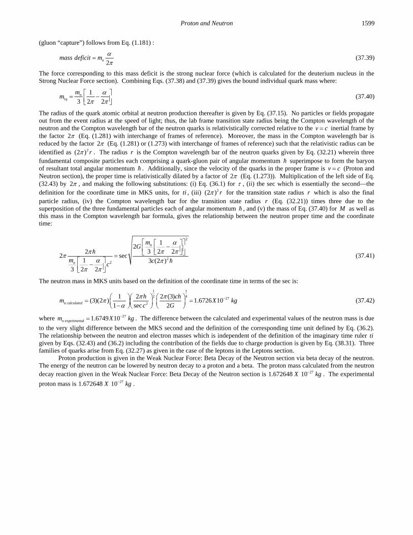
Proton and Neutron 1599
(gluon “capture”) follows from Eq. (1.181) :
2nmass deficit m
(37.39)
The force corresponding to this mass deficit is the strong nuclear force (which is calculated for the deuterium nucleus in the Strong Nuclear Force section). Combining Eqs. (37.38) and (37.39) gives the bound individual quark mass where:
1
1
3 2 2n
q
mm
(37.40)
The radius of the quark atomic orbital at neutron production thereafter is given by Eq. (37.15). No particles or fields propagate out from the event radius at the speed of light; thus, the lab frame transition state radius being the Compton wavelength of the neutron and the Compton wavelength bar of the neutron quarks is relativistically corrected relative to the v c inertial frame by the factor 2 (Eq. (1.281) with interchange of frames of reference). Moreover, the mass in the Compton wavelength bar is reduced by the factor 2 (Eq. (1.281) or (1.273) with interchange of frames of reference) such that the relativistic radius can be identified as 2(2 ) r . The radius r is the Compton wavelength bar of the neutron quarks given by Eq. (32.21) wherein three fundamental composite particles each comprising a quark-gluon pair of angular momentum superimpose to form the baryon of resultant total angular momentum . Additionally, since the velocity of the quarks in the proper frame is v c (Proton and Neutron section), the proper time is relativistically dilated by a factor of 2 (Eq. (1.273)). Multiplication of the left side of Eq. (32.43) by 2 , and making the following substitutions: (i) Eq. (36.1) for , (ii) the sec which is essentially the second—the definition for the coordinate time in MKS units, for ti , (iii) 2(2 ) r for the transition state radius r which is also the final particle radius, (iv) the Compton wavelength bar for the transition state radius r (Eq. (32.21)) times three due to the superposition of the three fundamental particles each of angular momentum , and (v) the mass of Eq. (37.40) for M as well as this mass in the Compton wavelength bar formula, gives the relationship between the neutron proper time and the coordinate time:
2
22
12
3 2 222 sec
1 3 (2 )3 2 2
n
n
mG
m cc
(37.41)
The neutron mass in MKS units based on the definition of the coordinate time in terms of the sec is:
1 1
2 427
n 2
1 2 2 (3)(3)(2 ) 1.6726 10
1 sec 2calculated
h chm X kg
c G
(37.42)
where 27 n experimental 1.6749 10m X kg . The difference between the calculated and experimental values of the neutron mass is due
to the very slight difference between the MKS second and the definition of the corresponding time unit defined by Eq. (36.2). The relationship between the neutron and electron masses which is independent of the definition of the imaginary time ruler ti given by Eqs. (32.43) and (36.2) including the contribution of the fields due to charge production is given by Eq. (38.31). Three families of quarks arise from Eq. (32.27) as given in the case of the leptons in the Leptons section.
Proton production is given in the Weak Nuclear Force: Beta Decay of the Neutron section via beta decay of the neutron. The energy of the neutron can be lowered by neutron decay to a proton and a beta. The proton mass calculated from the neutron decay reaction given in the Weak Nuclear Force: Beta Decay of the Neutron section is 27
1.672648 10X kg . The experimental
proton mass is 27 1.672648 10X kg .

Chapter 37 1600
INTERMEDIATE VECTOR AND HIGGS BOSONS The only fundamental matter particles that can exist are the three leptons, three sets of quarks, and their antiparticles. However, linear combinations of these fundamental particles may comprise more complicated species beyond neutrons and protons. Particle energies in collisions may exceed the particle production energies and consequently exceed the corresponding spacetime resonance frequencies during particle production and decay reactions. The relationship between proper and coordinate time has higher order or over-energy resonances due to the same principles regarding the relationship between proper and coordinate time that is the basis of production of the fundamental particles. Then, an increase in the intensity of particle reactions events is predicted at the over-energy resonance frequencies. However, the associated peak at the resonance energy does not represent a new fundamental particle. Nor, does this phenomenon have any association with mediating forces such as the weak nuclear force or the conveyance of inertial mass. The former is due to the electromagnetic force and the latter is due to the absolute nature of spacetime and the conservation of matter, energy, and spacetime with satisfaction of Maxwell’s equations and the conditions inherent in the Schwarzschild metric of spacetime required for particle production.
The additional resonances can be predicted by applying these principles to energy exceeding the production energy of a given particle. Specifically, using the spatial dimensions and the velocity at the electron production event, the scaling factor between the proper and coordinate time is given by Eq. (34.62) wherein the latter is imaginary because energy transitions are spacelike due to spacetime expansion from matter to energy conversion:
12 2sec
2C C
ge
C
ivGm
(37.43)
where gv is Newtonian gravitational velocity (Eq. (34.30)). Consider the muon that is a lepton arising from a resonance
involving the electron wherein in addition to pair production, the latter is a product of beta decay. The correction between proper and coordinate time based on the Coulombic potential as the basis of the muonic production energy is 2 (Eqs. (36.5) and (1.281)), and further applying Eq. (34.62) , the resonance coupling factor Cg is:
12Cg (37.44)
Using the relationship between the proper time and the electron coordinate time for the Coulomb potential energy as the production energy, the mass of the muon/antimuon using the MKS second is (Eqs. (36.5-36.6)):
1
328
2
11.8874 10 0.10587
2 sece
m X kg GeVc Gm
(37.45)
Applying resonance coupling factor Cg (Eq. (37.44)) to the muon production mass (Eq. (37.45)) having its inherent lepton
member, the electron, gives an over-energy resonance 0ZE at:
0
1
31 1
2
12 2 0.10587 91.16
2 secCZ
e
E g m GeV GeVc Gm
(37.46)
Experimentally, the event excess called the intermediate vector boson 0Z occurs at 91.1876 GeV [8]. This signature is deemed a manifestation of the weak force regarding an ad hoc postulated Standard Model treatment of beta decay.
In contrast, based on Maxwell’s equations and the conditions inherent in the Schwarzschild metric of spacetime required for particle production, the neutron mass is given by Eq. (37.42) in terms of fundamental constants and MKS units based on the definition of the coordinate time in terms of the sec. An over-energy absolute spacetime resonance of the electrically neutral neutron 0H
E due to the relationship between proper and coordinate time given by Eq. (37.43) is predicted at:
0
1 1
2 41 1 1
2
1 2 2 (3)(3)(2 ) 0.93956536 128.75
1 sec 2nH
h chE m GeV GeV
c G
(37.47)
High-energy proton-proton collisions that produce neutron-antineutron pairs decay to two gamma ray photons or correspondingly two pairs of electron-positron or muon-antimuon pairs. Such an excess of events at 126 GeV has recently been announced by CERN [9]. Specifically, the corresponding excess of events at the neutron over-energy spacetime resonance energy has been announced as the discovery the Higgs boson 0H that conveys mass to particles according to an ad hoc postulate of the Standard Model. However, there is no physical evidence that this slight excess of events at 126 GeV conveys mass to particles, and the energy of the excess events deemed the Higgs boson cannot and was not directly observed as a real particle due to the extraordinarily small mean lifetime of the resonance.
As given in the Weak Nuclear Force: Beta Decay of the Neutron section, a proton is formed via beta decay of the neutron. This requires the initial step of the conversion of a down quark to an up quark having charges -2/3 and +1/3, respectively, with the concomitant formation of an electron of the lepton family having a charge of -1. Considering that the

Proton and Neutron 1601
transition occurs on a time scale of 2510 s , the radius of the baryon is unchanged, and the energy change is that of electric energy decrease given by Eq. (1.170). Using 1/3, the magnitude of the change in charge normalized to that of the proton, and
22
, the relativistic correction term of the neutron production condition of Eq. (37.41) with the equivalence of the correction
for charge and mass density since they are interchangeable by the ratio /e m , an over-energy resonance W
E corresponding to
0ZE of Eq. (37.46) is predicted at:
12 2
32 212
221
1 1 11 1 2 2 1 1 2
3 32 sec
1 2 0.10587 1 1 2 80.51
3
CWe
E g mc Gm
GeV GeV
(37.48)
Then, by the symmetry of antiparticles, the positron decay of the antineutron corresponds to W . Experimentally, the event excess called the intermediate vector bosons W occurs at 80.423 GeV [8]. These particles convey the weak nuclear force according to an ad hoc postulate of the Standard Model that seems nonsensical since each weighs 80 times the mass of the neutron. There is no physical evidence that these particles produce a nuclear force. Moreover, the intermediate vector bosons W are not real particles in that they cannot and were not directly observed since the experimental mean lifetime of the resonance is 253.076 10 X s [10]. Similarly the experimental mean lifetime of the 0Z spacetime resonance is
252.6379 10 X s [11].
REFERENCES 1. R. Hasty et al., “Strange magnetism and the anapole structure of the proton,” Science, Vol. 290, (2000), pp. 2117-2119. 2. E. S. Ageev et al., “Measurement of the spin structure of the deuteron in the DIS region,” Phys. Lett. B, Vol. 612, (2005), pp.
154-164. 3. K. K. Seth, D. J. Hughes, R. L. Zimmerman, R. C. Grant, “Nuclear radii by scattering of low-energy neutrons,” Phys. Rev.,
Vol. 110, No. 3, (1958), pp. 692-700. 4. P. Weiss, “New probe reveals unfamiliar inner proton,” Science News, Vol. 159, May, 5, (2001), p. 277. 5. M. K. Jones, et al., “ /
p pE MG G ratio by polarization transfer in ep ep
,” Physical Review Letters, Vol. 84, No. 7, February,
14, (2000), pp. 1398-1402. 6. D. A. McQuarrie, Quantum Chemistry, University Science Books, Mill Valley, CA, (1983), pp. 238-241. 7. G. R. Fowles, Analytical Mechanics, Third Edition, Holt, Rinehart, and Winston, New York, (1977), pp. 195-196. 8. K. Hagiwara, et al., (Particle Data Group), Phys Rev. D, Vol. 66, 010001, (2002) (URL:http://pdg.lbl.gov). 9. “CERN experiments observe particle consistent with long-sought Higgs boson,” CERN press release, 4 July 2012,
http://press.web.cern.ch/press/PressReleases/Releases2012/PR17.12E.html. 10. http://www.wolframalpha.com/input/?i=W+boson. 11. http://www.wolframalpha.com/input/?i=Z+boson.

Chapter 37 1602

1603
Chapter 38 QUARKS Only three quark families can be formed from photons corresponding to the Planck equation energy, the potential energy, and the magnetic energy, where each is equal to the mass energy (Eq. (32.27)). As opposed to a continuum of energies, fundamental quark families arise from photons of only three energies. The considerations for the production of baryons are described in the Neutron and Proton Production section. Consider the relativistic corrections of the variables of the relationship between the proper and coordinate times, Eq. (32.43), for the production of three types of neutral baryon/antibaryon pairs, each comprised of three quarks and three gluons. The charges of each set of three quarks must sum to zero and the lowest energy nonuniform
spherical harmonics are those corresponding to = 1; thus, the charges are 1
3 ,
1
3 , and
2
3 for the baryon quarks and
1
3 ,
1
3 ,
2
3 for the antibaryon quarks. The radius of the quark atomic orbital at baryon production and thereafter follows from by
Eq. (37.15). The baryon possesses three quarks of total mass 2
Bm
(Eq. (37.16)); thus, the mass of each quark is:
1 (3)2B
q
mm
(38.1)
The quarks/gluons possess magnetic stored energy. Concomitant with the “capture” of the gluons by the quark resonator cavity, the magnetic flux of the gluons is “captured.” To conserve the total quark angular momentum, , the flux is trapped in quanta of the magnetic quantum of flux (See Electron g Factor section.). The quark/gluon velocity is v c ; thus, the magnetic stored energy is 2
Bm c (Eq. (29.14) and (29.15) with em replaced by Bm ). The mass (energy) released due to magnetic flux “capture”
(gluon “capture”) follows from Eq. (1.181).
2Bmass deficit m
(38.2)
The force corresponding to this mass deficit is the strong nuclear force (which is calculated for the deuterium nucleus in the Strong Nuclear Force section). Combining Eqs. (38.1) and (38.2) gives the bound individual quark mass:
1
1
3 2 2B
q
mm
(38.3)
No particles or fields propagate out from the event radius at the speed of light; thus, the lab frame transition state radius being the Compton wavelength of the neutron and the Compton wavelength bar of the neutron quarks is relativistically corrected relative to the v c inertial frame by the factor 2 (Eq. (1.281) with interchange of frames of reference). Moreover, the mass in the Compton wavelength bar is reduced by the factor 2 (Eq. (1.281) or (1.273) with interchange of frames of reference) such that the relativistic radius can be identified as 2(2 ) r . The radius r is the Compton wavelength bar of the neutron quarks given by Eq. (32.21) wherein three fundamental composite particles each comprising a quark-gluon pair of angular momentum superimpose to form the baryon of resultant total angular momentum . Additionally, since the velocity of the quarks in the proper frame is v c (Proton and Neutron section), the proper time is relativistically dilated by a factor of 2 (Eq. (1.273)). Multiplication of the left side of Eq. (32.43) by 2 , and making the following substitutions: (i) Eq. (36.1) for , (ii) the sec which is essentially the second—the definition for the coordinate time in MKS units, for ti , (iii) 2(2 ) r for the transition state radius r which is also the final particle radius, (iv) the Compton wavelength bar for the transition state radius r (Eq. (32.21))

Chapter 38 1604
times three due to the superposition of the three fundamental particles each of angular momentum , gives the relationship between the neutron proper time and the coordinate time:
2
2
12
3 2 222 sec
1 3 (2 )3 2 2
B
B
mGM
m cc
(38.4)
The mass of each member of a quark pair corresponds to an energy of Eq. (32.32) where the production state goes through the corresponding neutron comprising quarks and gluons. The down-down-up neutron (ddu) and anti-ddu correspond to the Planck equation energy. The strange-strange-charm neutron (ssc) and anti-ssc correspond to the electric energy. And, the bottom-bottom-top neutron (bbt) and anti-bbt correspond to the magnetic energy. It is shown that the masses are given by Eq. (32.43) and the relative masses differ in their specific function of the fine structure constant only. These functions are determined by relativistic coefficients in Eq. (38.4) given by Eq. (32.32) according to the kind of energy that is responsible for the respective level ( ddu , ssc , bbt ) of the particular particle within its family. DOWN-DOWN-UP NEUTRON (DDU) The down-down-up neutron is comprised of a down, down, and an up quark where the charge of a down quark is
1
3e , and the
charge of an up quark is 2
3e . The mass of the down-down-up neutron corresponds to the Planck equation energy given by Eq.
(32.28). Substitution of the mass of Eq. (38.3) for M as well as this mass in the Compton wavelength bar formula, gives the relationship between the down-down-up neutron proper time and the coordinate time:
2
22
12
3 2 222 sec
1 3 (2 )3 2 2
ddu
ddu
mG
m cc
(38.5)
The neutron mass in MKS units based on the definition of the coordinate time in terms of the sec is:
1 1
2 4
2
1 2 2 (3)(3)(2 )
1 sec 2ddu calculated
h chm
c G
(38.6)
27 1.6726 10ddu calculatedm X kg (38.7)
27 exp 1.6749 10ddu erimentalm X kg (38.8)
The difference between the calculated and experimental values of the neutron mass is due to the very slight difference between the MKS second and the definition of the corresponding time unit defined by Eq. (36.2) and the slight contribution due to the field energies of the quarks’ charges. The relation between the ddu neutron and electron masses which is independent of the definition of the imaginary time ruler ti given by Eqs. (32.43) and (36.2) including the contribution of the fields due to charge production is given by Eq. (38.31). STRANGE-STRANGE-CHARM NEUTRON (SSC) The strange-strange-charm neutron is comprised of a strange, strange, and a charm quark where the charge of a strange quark is
1
3e , and the charge of a charm quark is
2
3e . Given that the down-down-up neutron is a solution to Eq. (38.4), other
solutions follow from this solution and the other energy solutions. Consider the case of the potential energy. Given that the down-down-up neutron is “allowed” by the Planck energy
equation (Eq. (32.28)) and that the proper time is given by general relativity (Eq. (32.38)), the strange-strange-charm neutron mass can be calculated from the potential energy, V , (Eq. (32.27)) and the proper time relative to the down-down-up neutron inertial frame.
Baryons comprised of charm and strange quarks (antiquarks) decay to baryons of up and down quarks (antiquarks) and may be considered a transient resonance which decays to the stable baryons, the neutron or proton (antineutron or antiproton). For the lab inertial frame, the relativistic correction of the radius of the transition state atomic orbital given by the potential energy equations (Eq. (29.10) and (29.11)) is 2 . As shown in the Muon-Antimuon Lepton Pair section, for the down-down-up neutron inertial frame, the relativistic correction of the gravitational radius gr (Eq. (32.36)) relative to the proper frame is the
inverse, 2 . Furthermore, the potential energy equation gives an electrostatic energy; thus, the down-down-up neutron inertial time must be corrected by the relativistic factor of 2 relative to the proper time. (See the Special Relativistic Correction to the Ionization Energies section.) Multiplication of the right side of Eq. (38.4) by 2 and substitution of (i) gr , the relativistically

Quarks 1605
corrected gravitational radius for gr (Eq. (32.36)), and (ii) ddum , the mass of the down-down-up neutron, for M into Eq. (38.4)
gives the relationship between the proper time and the down-down-up neutron coordinate time:
2
22
12
3 2 222 2 sec
1 3 (2 )3 2 2
sscddu
ssc
mG m
m cc
(38.9)
The strange-strange-charm neutron mass in MKS units based on the definition of the coordinate time in terms of the sec is:
1233
2 2
1 2 (3)(3)(2 )
1 sec 2ssc calculatedddu
h chm
c m G
(38.10)
27 2 4.89 10 2.74 /ssc calculatedm X kg GeV c (38.11)
The observed mass of the hyperon that contains three strange quarks (sss) is [1]: 21673 /m MeV c
(38.12)
Thus, an estimate for the dynamical mass of the strange quark, sm , is:
2
21673 /558 /
3 3s
m MeV cm MeV c
(38.13)
The dynamical mass of the charm quark, cm , has been determined by fitting quarkonia spectra, and from the observed masses of
the charm pseudoscalar mesons 0 1865D and 1869D [2]:
21.580 /cm GeV c (38.14)
Thus, 2 2
exp 2 2(558 / ) 1580 /ssc erimental s cm m m MeV c MeV c (38.15)
2exp 2.70 /ssc erimentalm GeV c (38.16)
Eqs. (38.11) and (38.16) are in agreement. BOTTOM-BOTTOM-TOP NEUTRON (BBT) The bottom-bottom-top neutron is comprised of a bottom, bottom, and a top quark where the charge of a bottom quark is
1
3e ,
and the charge of a top quark is 2
3e . Given that the down-down-up neutron is a solution to Eq. (38.4), other solutions follow
from this solution and the other energy solutions. Consider the case of the magnetic energy. Given that the down-down-up neutron is “allowed” by the Planck energy
equation (Eq. (32.28)) and that the proper time is given by general relativity (Eq. (32.38)), the bottom-bottom-top neutron mass can be calculated from the magnetic energy (Eq. (32.27)) and the proper time relative to the down-down-up neutron inertial frame. As given in the Proton and Neutron section for the neutron and proton, the bottom-bottom-top neutron and the antibottom-bottom-top neutron radius, r , is given by the Compton wavelength:
,
C bbtbbt
hr
m c (38.17)
Furthermore, the transition state comprises two magnetic moments. For v c , the magnetic energy equals the potential energy, equals the Planck equation energy, equals 2mc . The magnetic energy is given by the square of the magnetic field as given by Eqs. (1.154-1.162). As in the case of the tau-mass calculation given in the Leptons sections, the magnetic energy corresponding to particle production is given by Eq. (32.32). Because two magnetic moments are produced, the magnetic energy (and corresponding photon frequency) in the proper frame is two times that of the down-down-up neutron frame. Thus, the down-down-up neutron time is corrected by a factor of two relative to the proper time. Both the bottom-bottom-top neutron and the antibottom-bottom-top neutron undergo and exit the production event with a radius given by Eq. (38.17). Whereas, in the case of tau-antitau production given in the Leptons section, the radius of the lepton and antilepton increased symmetrically to produce lepton plane waves at infinity relative to each other. Thus, in the lab frame, the gravitational radius gr (Eq. (32.36)) is not
corrected by 2(2 ) . Furthermore, a mutual central magnetic field exists for the particles of fixed radius. The corresponding electrodynamic special relativistic correction is given by Eqs. (1.241-1.260) where the mass of each particle in Eq. (1.255) is
bbtm . Thus, as a consequence of the mutual magnetic dipole interaction, the mass bbtm is replaced by the corresponding reduced
mass bbt of the two baryonic magnetic dipoles:
2bbt
bbt
m (38.18)
Furthermore, for the lab inertial frame, the relativistic correction of the radius of the transition state atomic orbital given by the

Chapter 38 1606
magnetic energy equations (Eq. (29.14) and (29.15)) is 4
1
. As shown in the Tau-Antitau Lepton Pair section, for the down-
down-up neutron inertial frame, the relativistic correction of the gravitational radius gr relative to the proper frame is the
inverse, 4 . Multiplication of the right side of Eq. (38.4) by 2 and substitution of (i) ddum , the mass of the down-down-up
neutron, for M , (ii) 4gr , the relativistically corrected gravitational radius for gr (Eq. (32.36)), and (iii) the reduced mass bbt
(Eq. (38.18)) for bbtm into Eq. (38.4) gives the relationship between the proper time and the down-down-up neutron coordinate
time:
4
22
12
3 2 222 2sec
1 3 2(2 )3 2 2
bbtddu
bbt
mG m
m cc
(38.19)
The bottom-bottom-top neutron mass in MKS units based on the definition of the coordinate time in terms of the sec is:
1233
2 4
1 2 2 (3)(3)(2 )
1 2secbbt calculatedddu
h chm
c m G
(38.20)
25 2 3.50 10 196 /bbt calculatedm X kg GeV c
The dynamical mass of the bottom quark, bm , has been determined by fitting quarkonia spectra; and from the observed masses
of the bottom pseudoscalar mesons 0 5275B and 5271B [2]:
24.580 /bm GeV c (38.21)
Thus, the predicted dynamical mass of the top quark based on the dynamical mass of the bottom quark is: 2 2
2 196 / 2(4.580 / )t calculated bbt calculated bm m m GeV c GeV c (38.22)
2 187 /t calculatedm GeV c
Considering all jets, the CDF collaboration determined the mass of the top quark to be 2186 10 /GeV c [3]. All other hadrons comprise linear combinations of the fundamental quarks.
RELATIONS BETWEEN MEMBERS OF THE NEUTRON FAMILY AND THE LEPTONS As shown in the Leptons section (Eqs. (36.9-36.11)), the mass ratios of the members of the lepton family are based solely on the fine structure constant . Based on Eqs. (36.3), (38.6), (38.10), and (38.20), the relations between the electron and neutron masses which are independent of the definition of the imaginary time ruler ti given by Eq. (32.43) are [4]:
212 3
1838.061
N
e
m
m
1838.68 (38.23)
1
3
2
1 12.926
2 3ssc ssc
ddu N
m m
m m
(38.24)
12 3
2
271.8bbt
ssc
m
m
(38.25)
1
3
4
1210
12bbt bbt
ddu N
m m
m m
(38.26)
The respective experimental neutron/electron mass ratio according to the 1998 CODATA is given in parentheses [5]. Remarkably, all of the quarks as well as leptons are related by the fine structure constant only which demonstrates that the masses arise as a consequence of special relativity. This result is analogous to the magnetic field that is a special relativistic consequence of the electric field.
Eq. (38.23) does not include the electron neutrino energy or the coulomb and magnetic field energies. As shown in the Relations Between the Leptons section, in order to conserve mass-energy, the electromagnetic fields of the particles must be included in the mass determination. The correction * to the electron mass given by Eq. (36.15) is:
12
* 1 22
(38.27)
Similar to the electron-positron pair, the ddu-neutron-anti-ddu-neutron pair depends on the Plank energy equation. The latter is exceptional in that the radius of the charged quarks does not change following particle production. Since the energy in the electrostatic fields of the electron-positron pair are released as photons during binding and photons have no gravitational mass as

Quarks 1607
shown in the Gravity section, the relativistic correction decreases each lepton mass as shown in Eq. (36.15). However, in the case of the neutron, the electrostatic field, for radial distance greater than the radius of the quarks, is zero, and the gluons result in a relativistically corrected quark mass as given in the Proton and Neutron section. In this case, the corresponding correction
* has the opposite sign as that of Eq. (38.27) and is given by:
12
* 1 22
(38.28)
Substitution of the relationship between the definition of the imaginary time ruler ti given by Eq. (36.4) and the correction due to the contribution of the fields due to charged quark production given by Eq. (38.28) into Eq. (38.6) gives the ddu neutron mass as:
1 1 122 4
2
1 2 2 (3)(3)(2 ) 1 2
1 0.9975(46714) MKS second 2 2ddu calculated
h chm
c G
(38.29)
27 1.6749 10ddu calculatedm X kg (38.30)
To the appropriate number of significant figures, there is good agreement with the experimental value of 27
experimental 1.6749 10ddum X kg .
Based on Eqs. (36.3), (38.6), (38.27), and (38.28), the relation between the ddu neutron and electron masses (Eq. ((38.23)) which is independent of the definition of the imaginary time ruler ti given by Eq. (36.43) including the contribution of the fields due to charge production is:
2
2
2
1 2212 3
1838.671
1 22
N
e
m
m
1838.68 (38.31)
The experimental ddu neutron-electron mass ratio according to the 1998 CODATA given in parentheses matches the predicted value very well.
REFERENCES 1. I. S. Hughes, Elementary Particles, Cambridge University Press, (1972), pp. 124-125. 2. I. R. Kenyon, Elementary Particle Physics, Routledge & Kegan Paul, London, (1987), p.196. 3. K. Hagiwara et al., Phys. Rev. D66, 010001 (2002); http://pdg.lbl.gov; http://pdg.lbl.gov/2002/topquark_q007.pdf. 4. Personal communication, Dr.-Ing. Günther Landvogt, Hamburg, Germany, February, (2003). 5. P. J. Mohr and B. N. Taylor, “CODATA recommended values of the fundamental physical constants: 1998,” Reviews of
Modern Physics, Vol. 72, No. 2, April, (2000), pp. 351-495.

Chapter 38 1608

1609
Chapter 39 NUCLEAR FORCES AND RADIOACTIVITY THE WEAK NUCLEAR FORCE: BETA DECAY OF THE NEUTRON BETA DECAY ENERGY The nuclear reaction for the beta decay of a neutron is: 1 1
en H (39.1)
where e is the electron antineutrino. The beta decay energy, E , can be calculated from conservation of mass-energy
n p eE E E E (39.2)
where nE , pE , and eE are the mass-energy of the neutron, proton, and electron. Thus,
2 ( ) 0.7824beta decay n P eE m m m c MeV (39.3)
The experimental value is 0.782 MeV [1].
Neutron decay results in the change of the nuclear moment from that of a neutron 4 3
1 29 25 N
to that of a
proton 4
( 2 )9 N where these terms were determined in the Magnetic Moment section. The radii of the proton and the neutron
are the corresponding Compton wavelengths given by Eqs. (37.3) and (37.15), respectively:
150 , 1
21.32141 10e
C p pP
a mX m r
m
(39.4)
150 , 1
21.31959 10e
C n nN
a mX m r
m
(39.5)
The beta decay energy can be calculated from the magnetic, electric, and kinetic energy transformations which occur during the decay. The energy components are the sum of the following:
• the release of magE , the magnetic energy stored in one N , since the corresponding beta particle no longer contains the
magnetic fields of the gluons at a radius of ,C p , the radius of the proton, following beta decay;
• minus magE (gluon), the energy to change the gluon field corresponding to a down quark to that corresponding to an up
quark; • minus eleE , the electric energy stored in the electric field of the proton;
• minus , ,,C n C pvE , the electric potential energy change in going from the radius of the neutron to that of the proton;
• plus T , the initial kinetic energy of the electron in its frame at production with v c at a radius of the electron
Compton wavelength bar.
The magnitude of the beta decay energy contributions are given as follows:

Chapter 39 1610
From the Strong Nuclear Force section, and using Eq. (37.39) with Eqs. (33.13) and (39.40), magE is given by:
2 6 1.089727 10
2mag pE m c X eV
(39.6)
Since the change in the magnetic moment contribution of quark/gluon function is 3
25 (Eq. (37.36)) and the change in the energy
stored in the magnetic field is proportional to the change in magnetic moment squared (Eq. (1.154)), magE (gluon) is given by:
2
43( ) 1.569207 10
25mag magE gluon E X eV
(39.7)
where magE is given by Eq. (39.6). From Eqs. (1.264) and (39.5), eleE is given by:
2
5
0 ,
5.456145 108ele
C n
eE X eV
(39.8)
From Eqs. (1.261), (39.4), and (39.5), , ,,C n C pvE is given by:
, ,
2
,
0 , ,
1 11502.2
4C n C pv
C n C p
eE eV
(39.9)
From the Creation of Matter from Energy and Pair Production sections, and using Eq. (1.35), T is given by:
22
2 2 5 22
01
1 1 1 12.555017 10
2 2 2 22
2
ee e
e CN e
N
mT mv m m c X eV
mm a m
m
(39.10)
wherein the electron Compton wavelength bar is given by Eq. (28.7). The beta decay energy, E , given by the sum of the
energies of Eqs. (39.6-39.10) is:
, ,,( )
0.7824
C n C pmag mag ele vE E E gluon E E T
E MeV
(39.11)
The calculated result is in good agreement with Eq. (39.3). Then the weak force is the negative gradient of the weak energy given by Eq. (39.11). NEUTRINOS Photons carry of angular momentum in their electric and magnetic fields as shown in the Photon section. All electronic
transitions require of angular momentum photons. Nuclear reactions such as beta decay require emission of neutrinos with 2
of angular momentum. Thus, they may be photons with different electric and magnetic fields that give 2
of angular
momentum. Then different trigonometric functions of the electric and magnetic fields would correspond to the different flavor neutrinos, the energy of each would depend on its frequency since the speed is light speed, and the cross sections would depend on the particular fields and energy.
To conserve energy and linear and angular momentum an electron antineutrino, e , is emitted with the beta particle. The
antineutrino is a unique elliptically polarized photon that has handedness (the neutrino and antineutrino have opposite handedness), is massless, and travels at the speed c . Consider the photon atomic orbital given in the Equation of the Photon section. It may comprise magnetic and electric field lines basis elements that are constant in magnitude as a function of angle over the surface. Or, the magnitude may vary as a function of angular position ( , ) on the atomic orbital which corresponds to an elliptically polarized photon. The general photon equation for the electric field is
0, 02
0
11 , Re ,
4 2nim tm
photon
eY Y e r
r n
E (39.12)
For the particle-production or emission event, photonr is the radius of the photon atomic orbital which is equal to Hna , the
change in electron atomic orbital radius given by Eq. (2.21), is the photon wavelength which is equal to , the change in
the de Broglie wavelength of the atomic orbital given by Eqs. (2.21), (1.34), and (1.38), and 2
n
c
is the photon angular
velocity which is equal to , the change in atomic orbital angular velocity given by Eqs. (2.21). The magnetic field photon

Nuclear Forces and Radioactivity 1611
atomic orbital is given by Eqs. (4.14) and (4.2). The nature of the unique elliptically polarized photon atomic orbital which is the antineutrino (neutrino) is determined by the nature of quark/gluon functions and the change in the quark/gluon angular harmonic functions during the transition from a neutron to a proton (proton to a neutron) with the emission of a beta particle (positron). A free quark or a free gluon is not a stable state of matter, and both are precluded from existence in isolation. Quarks and gluons can only exist in pairs, each comprising a quark and a gluon. In the case of beta decay, a down quark/gluon is converted to an up quark/gluon. Energy and linear momentum are conserved by the emission of an electron antineutrino, e ,
with the beta particle where the maximum energy of the antineutrino is that of the mass deficit. To conserve angular momentum, the electric field, E , of the electron antineutrino has an angular dependence given by a harmonic function squared
corresponding to the change between the initial and final quark/gluon functions where the electric field of each gluon and its corresponding quark are radial and Eq. (37.34) applies.
2
2
Re , 12
1 cos 2 cos Re 1 Re 1
2 2 2 2
n
n n
i tm
i t i t
Y e r
e r e r
E
(39.13)
where 1 and the power is given by Eq. (4.16). In contrast, the electric field of a photon corresponding to electronic transitions (Eq. (39.12)) is given by the sum of a constant function plus a spherical harmonic modulation function which
averages to zero over a period. The angular momentum of an antineutrino (neutrino) is 2
(2
)
41Re ( )
8 2dx
c m r E B*
(39.14)
compared to that of a photon corresponding to an electronic transition of (Eq. (4.1)). The matrices to generate the electric and magnetic vector fields (e&mvf) of neutrinos are the same as those of the right-
and left-circularly-polarized and linearly-polarized photons with the exception that the magnitude of the basis element field is not constant over the spherical surface, but is modulated by a trigonometric function squared. The right- and left- 2cos or
2sin -polarized neutrinos are mirror images of opposite spin corresponding to a neutrino-antineutrino pair. The right-hand-2cos -polarized neutrino ( 2RHC P ) is given by:
20 0
20
Red
'
& cos '
'
1 cos 1 cos sin
2 2 2 2 2 01 cos 1 cos sin
cos cos2 2 2 2 2
sinsin sin
cos2 2
photon n
n
x
e mvf E B y
z
r r E r
r
0
Blue
cos
0
sin
n
n
r
B
r
(39.15)
The 2RHC P neutrino-e&mvf that is generated by the rotation of the great-circle basis elements in the xz- and yz-planes about
the , ,0x y zi i i -axis by 2
corresponding to the output of the matrix given by Eq. (39.15) is shown in Figure 39.1 wherein the
magnitude of each field line is according to 2cos .

Chapter 39 1612
Figure 39.1. The field-line pattern given by Eq. (39.15) from three orthogonal perspectives of a 2RHC P neutrino-e&mvf corresponding to the first great circle magnetic field line and the second great circle electric field line shown with 6 degree increments of the angle . (Electric field lines red; Magnetic field lines blue).
The corresponding antineutrino, the left-hand- 2cos -polarized neutrino ( 2LHC P ), is given by is given by:
20 0
2
'
& cos '
'
1 cos 1 cos sin
2 2 2 2 2 01 cos 1 cos sin
cos cos2 2 2 2 2
sinsin sin
cos2 2
photon n
n
x
e mvf E B y
z
r r r
r
Red Blue
cos
0
sin
n
n
r
r
(39.16)
The 2LHC P neutrino-e&mvf that is generated by the rotation of the great-circle basis elements in the xz- and yz-planes about
the , ,0x y zi i i -axis by 2
corresponding to the output of the matrix given by Eq. (39.16) is shown in Figure 39.2.
Figure 39.2. The field-line pattern given by Eq. (39.16) from three orthogonal perspectives of a 2LHC P neutrino-e&mvf corresponding to the first great circle magnetic field line and the second great circle electric field line shown with 6 degree increments of the angle . (Electric field lines red; Magnetic field lines blue).

Nuclear Forces and Radioactivity 1613
Based on the invariance of the field lines under Gauss’ Integral Law as given in the Photon section, the spatial distribution of the field lines of a cosine-squared neutrino (Eq. (39.13)) in the inertial frame for the stationary observer or laboratory frame is shown in Figure 39.3.
Figure 39.3. The electric (red) and magnetic (blue) field lines of a cosine-squared neutrino given by Eq. (39.13) as seen along the axis of propagation in the lab inertial reference frame at a fixed time. A and B. Views transverse to the axis of propagation, the z-axis, wherein 2 neutrinor . C and D. Off z-axis views showing field aspects both along and transverse to the
axis of propagation.
Eq. (39.13) is the equation of the neutrino’s electric field in its frame. The neutrinos fields called the neutrino electric and magnetic vector field (neutrino-e&mvf) follows from that of the photon. Eq. (25) of Appendix V: Analytical-Equation Derivation of the Photon Electric and Magnetic Fields which gives the laboratory-frame relationship of the fields and the angular momentum then becomes:
2
3 2 2 40 0
0 0
1 22 sin 2 cos sin
8 4 2 2photon
Er d
c
(39.17)
22
3 20 0
0 0
2 1 cos 2 1 cos 2sin 2
32 2 2 2photon
Er d
c
(39.18)
2
3 2 2 30 0
0 0
2sin 2 1 cos 2 cos 2 cos 2
256 2photon
Er d
c
(39.19)
Using the wave equation relationship and the relationship between the wavelength and the radius of the photon-e&mvf given by Eq. (21) and Eq. (22) of Appendix V, respectively, gives
2 2
2 40 020 0
40 2 2 2 3
0 0
sin 2 sin 2 cos 2
128 2sin 2 cos 2 sin 2 cos 2
d dE
c
d d
(39.20)
The integrals by Lide [2] give
3
0 0
2 4 420 0
400 0
3
0
1 sin 2sin 4
2 8 6
sin 2 cos 264sin8
128 8 10 2
1cos 2
5
Ec
d
(39.21)
2 4
20 04 0
0 0 0
1sin 2 cos 2 2
128 2 8 30 2
Ec
(39.22)

Chapter 39 1614
2 4
0 04
0 0 0128 2 8 2
Ec
(39.23)
2 50
40
3
1024 2
Ec
(39.24)
Thus,
4
20 00 5 5
512 512
3 3E
c c
(39.25)
which has the required MKS units of 1Vm . From Plank’s law, the energy is given by:
2 50
40
3
2 1024
EE L c
(39.26)
In the case of Eq. (39.13), a neutrino of a different flavor can also have an electric field in its frame of:
2
2
Re , 12
1 cos 2 sin Re 1 Re 1
2 2 2 2
n
n n
i tm
i t i t
Y e r
e r e r
E
(39.27)
The right-hand- 2sin -polarized neutrino ( 2RHS P ) is given by:
20 0
2
Red
'
& sin '
'
1 cos 1 cos sin
2 2 2 2 2 01 cos 1 cos sin
sin cos2 2 2 2 2
sinsin sin
cos2 2
photon n
n
x
e mvf E B y
z
r
r r r
r
Blue
cos
0
sin
n
nr
(39.28)
The 2RHS P neutrino-e&mvf that is generated by the rotation of the great-circle basis elements in the xz- and yz-planes about
the , ,0x y zi i i -axis by 2
corresponding to the output of the matrix given by Eq. (39.28) is shown in Figure 39.4.
Figure 39.4. The field-line pattern given by Eq. (39.28) from three orthogonal perspectives of a 2RHS P neutrino-e&mvf corresponding to the first great circle magnetic field line and the second great circle electric field line shown with 6 degree increments of the angle . (Electric field lines red; Magnetic field lines blue).

Nuclear Forces and Radioactivity 1615
The corresponding antineutrino, the left-hand- 2sin -polarized neutrino ( 2LHS P ), is given by is given by:
20 0
2
'
& sin '
'
1 cos 1 cos sin
2 2 2 2 2 01 cos 1 cos sin
sin cos2 2 2 2 2
sinsin sin
cos2 2
photon n
n
x
e mvf E B y
z
r r r
r
Red Blue
cos
0
sin
n
n
r
r
(39.29)
The 2LHS P neutrino-e&mvf that is generated by the rotation of the great-circle basis elements in the xz- and yz-planes about
the , ,0x y zi i i -axis by 2
corresponding to the output of the matrix given by Eq. (39.29) is shown in Figure 39.5.
Figure 39.5. The field-line pattern given by Eq. (39.29) from three orthogonal perspectives of a 2LHS P neutrino-e&mvf corresponding to the first great circle magnetic field line and the second great circle electric field line shown with 6 degree increments of the angle . (Electric field lines red; Magnetic field lines blue).
The spatial distribution of the field lines of a sine-squared neutrino (Eq. (39.27)) in the inertial frame for the stationary
observer or laboratory frame is shown in Figure 39.6.

Chapter 39 1616
Figure 39.6. The electric (red) and magnetic (blue) field lines of a sine-squared neutrino given by Eq. (39.27) as seen along the axis of propagation in the lab inertial reference frame at a fixed time. A and B. Views transverse to the axis of propagation, the z-axis, wherein 2 neutrinor . C and D. Off z-axis views showing field aspects both along and transverse to the axis of
propagation.
In this case, Eq. (25) of Appendix V: Analytical-Equation Derivation of the Photon Electric and Magnetic Fields then becomes:
2
3 2 60 0
0 0
1 22 sin 2 sin
8 4 2 2photon
Er d
c
(39.30)
32
3 20 0
0 0
2 1 cos 2sin 2
32 2 2photon
Er d
c
(39.31)
2
3 2 2 30 0
0 0
2sin 2 1 3cos 2 3cos 2 cos 2
256 2photon
Er d
c
(39.32)
Using the wave equation relationship and the relationship between the wavelength and the radius of the photon-e&mvf given by Eq. (21) and Eq. (22) of Appendix V, respectively, with the integral by Lide [2] gives
2 2
2 40 020 0
40 2 2 2 3
0 0
sin 2 3 sin 2 cos 2
128 23 sin 2 cos 2 sin 2 cos 2
d dE
c
d d
(39.33)
Using the integral #322 and #320 of Lide [2] gives
3
0 0
2 4 420 0
400 0
3
0
1 sin 2sin 4 3
2 8 6
sin 2 cos 23 64sin8
128 8 10 2
1cos 2
5
Ec
d
(39.34)
2 4
20 04 0
0 0 0
3 1sin 2 cos 2 2
128 2 8 30 2
Ec
(39.35)
2 4
0 04
0 0 0
3
128 2 8 2
Ec
(39.36)
2 50
40
7
1024 2
Ec
(39.37)

Nuclear Forces and Radioactivity 1617
Thus,
4
20 00 5 5
512 512
7 7E
c c
(39.38)
Due to its unusual angular momentum, the antineutrino and neutrino interact extremely weakly with matter. Essentially, it only has a finite cross-section for processes which involve transitions of two fundamental particles simultaneously. Such cases include beta decay, inverse beta decay, and the hydrino decay reaction (Eq. (32.173)).
1 He e
aH
p
(39.39)
where e is the electron neutrino and e is the electron antineutrino. There are three classes of neutrinos (antineutrinos)
corresponding to the electron (antielectron), muon (antimuon), and tau (antitau) as described in the Leptons section. Each flavor corresponds to its multipolarity and polarization, 2cos , 2sin , and the superposition of 2cos and 2sin . Its particle versus antiparticle type corresponds to its handedness. The determination of the flavor and type assignment can be determined by the multipolarity and polarization and handedness of the particle reaction that gives rise to the neutrino that conserves theses aspects as well as energy and linear momentum. The energy of the electric and magnetic fields given by Eq. (1.154) and Eq. (1.263), respectively, equals the energy given by the Planck equation (Eq. (4.8)). The multipolarities and polarizations of photons of visible light change upon interacting with a dichroic material through which they propagate. Similar to dichroism, interconversion of neutrinos may be possible via interaction with matter that causes corresponding changes in multipolarities and polarizations.
Thus, neutrinos are each a photon that has an exceptional 2
angular momentum in its electric and magnetic fields giving
rise to an intrinsic weak interaction limited to nuclei, travels at the speed of light, and can change polarization in condensed matter in a manner that may appear as “oscillation between flavors”. Light speed is characteristic of and identifies photons. Neutrinos have been confirmed to be photons by the measurement of the neutrino velocity with the OPERA detector to be the speed of light to within a relative difference of 52.48 0.28 0.30 10sat sys X [3]. Moreover, the speeds of photons and
neutrinos are identical within a part per billion from the coincidence of optical and neutrino detection of supernova 1987A [4]. THE STRONG NUCLEAR FORCE THE DEUTERIUM NUCLEUS The bonding in multi-nucleon nuclei involves the superposition of the quark and gluon functions of the constituent nucleons to form the nuclear version of atomic orbitals wherein the gluons provide the central force and the quarks comprise the two-dimensional current-density surfaces. The nuclear bonding gives rise to spherical shells comprising equipotential minimum-energy surfaces as a linear combination of the nucleons. For example, the deuterium nucleus is a minimum energy superposition of a neutron and a proton. Thus, the deuterium quark/gluon function is a spherical coordinate atomic orbital solution of Laplace’s equation (Eq. (I.44)). The neutron is electrically neutral; thus, no electric term arises in the energy calculation. The neutron and proton quarks of the same kind or flavor are indistinguishable and superimpose to form the deuterium atomic orbital. The gluon electric and magnetic fields of each nucleon superimpose with conservation of stored electric energy density (Eq. (1.263)) and stored magnetic energy density (Eq. (1.154)); however, gluon mass-energy is released as the proton and neutron gluon fields superimpose to provide the central field of the deuterium atomic orbital comprising the linear combination of quarks from both nucleons. The quark/gluons possess magnetic stored energy. Concomitant with the superposition of the neutron with the proton, the quark resonator cavity of the proton traps the magnetic flux of the neutron gluons, and the neutron quark resonator cavity captures the flux of the proton gluons. To conserve the total quark angular momentum of each nucleon, , the flux is trapped in quanta of the quantum of magnetic flux. As shown in the Quark and Gluon Functions of the Proton and Neutron section, the quark/gluon proper velocity is c . Therefore, the quark/gluon stored magnetic energy is 2
Pm c and 2Nm c for
the proton and the neutron, respectively (Eqs. (29.14) and (29.15) with em replaced by the nucleon mass). The energy released
due to the magnetic flux capture, the deuterium binding energy ( BindingE ), follows from Eq. (1.181) :
2
2 2Binding P NE m m c
(39.40)
2
2Binding P NE m m c
(39.41)
The calculated mass of deuterium is
1 2.014149 2e P NMass m m m AMU
(39.42)
The NIST experimental mass of deuterium is 2.0141017778 AMU [5].

Chapter 39 1618
NUCLEAR AND X-RAY MULTIPOLE RADIATION Using Maxwell’s equations, the essential features of multipole radiation in nuclei can be presented with simple arguments developed by Jackson [6]. By using Jackson’s Eq. (17.78) and the multipole coefficients (Jackson’s Eqs. (17.93) and (17.95)), the total power radiated by a multipole of order ( , m) is:
22 22
22 22
2 1( , )
[(2 1)!!]
2 1( , )
[(2 1)!!]
E m m
M m m
cP m k Q Q
cP m k M M
(39.43)
The transition probability (reciprocal mean life) is defined as the power divided by the energy of a photon:
1 P
(39.44)
Using the source structure given in the Proton and Neutron sections, the oscillating nuclear charge density of a nucleus comprised of many nucleons may be modeled as being of the form
3
3( , ),
(x)0,
m
eY
a
r a
r a
(39.45)
The corresponding electric multipole moment lmQ is:
3
3mQ ea
(39.46)
independent of m . Based on the spherical-shell structure of the nucleons, the divergences of the magnetizations is:
3
2( , ) ,1 r J
10,
m
g eY
a mcrc
M
r a
r a
(39.47)
where g is the effective g factor for the magnetic moments of the particles in the nuclear system, and /e mc is twice the Bohr magneton for those particles. The sum of magnetic multipole moments is:
2
2m m
gM M ea
mca
(39.48)
The definitions of the multipole moments mQ and mQ given by Jackson’s Eq. (17.94) are:
* 3m mQ r Y d x (39.49)
* 3
1m m
ikQ r Y d x
r M
(39.50)
Using Eqs. (39.48) and (39.50) gives:
2lm lmQ g Q
mc
(39.51)
Since the energies of radiative transitions in nuclei are always very small compared to the rest energies of the particles involved (i.e. 2mc ), mQ is always completely negligible compared to mQ . However, using Eqs. (39.43), (39.44), and (39.46), the
transition probability for electrical multipole transitions of order are:
22
22
1 2 1 3( )
( ) [(2 1)!!] 3E
eka
c
(39.52)
Using Eqs. (39.43), (39.44), (39.48), and (39.50–39.52), the transition probability for magnetic multipoles is:
2
22
1 123( ) ( )
3
g
mca
(39.53)
In the long-wavelength limit ( 1)ka , the transition rate predicted by Eq. (39.52) falls of rapidly with increasing multipole
order, for a fixed frequency due to the 2( ) lka factor in the transition probability. Consequently, the lowest nonvanishing

Nuclear Forces and Radioactivity 1619
multipole will generally be the only one having a significant rate in the radioactive decay. Omitting numerical factors of relative order (1/ ) , the ratio of transition probabilities for successive orders of either electric or magnetic multipoles of the same frequency is:
1 2
1 2
( 1) ( )
4( )
ka
(39.54)
The transition rates of electric dipole transitions of single-electron-excited-state atoms were given in the State Lifetimes and Line Intensities section. Consider an Auger transition due to a multipole central field created by an inner shell vacancy. The dimensions of the source due to the initial to final state current may be taken as having the same multipolarity as the central field and can be approximated as 0( / Z),a a where 0a is the Bohr radius and Z is the nuclear charge. The energy of any atomic
transition obeys, the relationship:
2
2
0
Ze
a
(39.55)
where the right-hand side of Eq. (39.55) only holds for one electron atoms as shown in the One-Electron Atom section, Two-Electron Atoms section, and Three- Through Twenty-Electron Atoms section. Thus, an estimate of ka is given by:
Zka
(39.56)
where is the fine structure constant. According to Eq. (39.54) the transition rates of successive multipoles have the ratio 2( Z) . Using 1
0 / Z ( / Z)a a mc in Eq. (39.53), the magnetic th multipole transition rate is about a factor of 2( Z)
smaller than the corresponding electric multipole rate. The electric dipole transitions are predicted to be the most intense, with
electric quadrupole and magnetic dipole transitions a factor 2Z weaker. Competition from transitions other than that of the
lowest-order electric multipole is only possible with X-ray transitions in heavy elements. Eq. (39.52) can be used to characterize radiative transitions in atomic nuclei as well, but the values of ka cover a wide
range because nuclear radiative transition energies vary greatly (from ~10 keV to several MeV). Consequently, for a given multipole order, the transition probabilities (or mean lifetimes) will range over many orders of magnitude depending on the energy release, overlapping the multipoles on either side. However, because of the strong dependency on , rate behavior at a fixed energy release can be obtained from Eqs. (39.52) and (39.53) that is useful in cataloging nuclear multipole transitions. Using Eq. (39.52) with the proton charge e and 135.6 x10a cm (nuclear radius appropriate to mass number A 100 ), a log-log plot of lifetimes of electric multipole transitions versus energy is shown in Figure 39.7. Although the curves tend to converge at high energies, the predicted lifetimes for different multipoles at the same energy differ by factors typically of order
510 that is permissive of assigning multipole orders. The experimentally observed lifetime-energy diagram [7] shows broad, but well-defined, bands lying in the vicinity of the straight lines shown in Figure 39.7. With Eq. (39.46) being an upper bound on the multipole moment, there is a general tendency for the corresponding estimate given by Eq. (39.52) to serve as a lower bound on the lifetime. But, for certain so-called “enhanced” electric quadrupole transitions the lifetimes can be much as 100 times shorter than those shown in Figure 39.7. Figure 39.7. Log-log plot of lifetimes of electric multipole transitions versus energy from Eq. (39.52).

Chapter 39 1620
Using a typical nucleon g factor of g~3 and source size of 1/3 131.2 10 a R A X cm in Eq. (39.53), the relationship between magnetic and electric multipoles of the same order is:
2/3
1 0.3 1
( ) A ( )M E
(39.57)
Since the numerical factor 2/3
0.3
A ranges from 2 -2 4 10 0.8 10 20 250X to X for A , given multipole order electric transitions
are predicted to be 25-120 times more intense than the magnetic transitions. For most multipoles, this relationship is experimentally confirmed. But, for 1 , there are special circumstances in nuclei at least at low energies whereby strongly attractive, charge-independent forces inhibit electric dipole transitions. In these cases, Eq. (39.57) does not hold, and magnetic dipole transitions are far commoner and equally intense as electric dipole transitions. The weak and strong nuclear forces given in the Beta Decay section and the Strong Nuclear Force section, respectively, are examples of where the magnetic energy is dominant and Eq. (39.57) with Eq. (39.46) does not apply.
Based on selection rules corresponding to conservation of angular momentum in the initial and final states and the radiation of multipolarity as shown in the Selection Rules section, a transition between two quantum states involving a mixture of multipoles, such as magnetic , ( 2),... pole and electric ( 1), ( 3),... pole, can occur. In the long-wavelength limit, only the lowest multipole of each type is significant. Combining the ratios (39.105) and (39.106) gives the relative transition rates of electric ( 1) pole to magnetic pole (most commonly used for 1 ):
21 1/3
1
( 1) A
[ ( )] 200M
E E
(39.58)
where E is the photon energy in MeV. For energetic transitions in heavy elements, the electric quadrupole amplitude is ~5 per cent of the magnetic dipole amplitude. If, there is an enhancement of the effective quadrupole moment by a factor of 10 as observed in the rare earth and transuranic nuclei, the electric quadrupole transition competes favorably with the magnetic dipole transition. Even for energetic transitions, a magnetic 1 pole never comes close to competing with an electric pole
because for a mixture, the ratio of transition rates is:
1 2
1
( 1)
600( )M
E
E
(39.59)
In addition to emission, resonant absorption of nuclear radiation is possible. The gluon fields of a nucleon such as a proton or a neutron are given in the Proton and Neutron section. A resonant photon having gamma-ray energy and of angular momentum in its electric and magnetic fields (Eq. (4.1)) can cause an excited nuclear state with a corresponding source-current component induced in the quarks of the same multipolarity as that of the gamma ray. The process is akin to that of the formation of an excited atomic state as given in the Excited States of the One-Electron Atom (Quantization) section. The absorption of a gamma ray gives rise to a trapped-photon standing wave inside the resonator cavity provided by the quarks of the nucleon. Both the photon standing wave and the source current to which it is phase-matched are spherical and time harmonics. The resonant absorption of gamma rays is the Mössbauer Effect. The nuclear size may increase or decrease depending on the effect of the excitation on the strong nuclear force via the absorbed photon field superposing with the gluon field. Similarly to the case of excited atomic states given in the Excited States of the One-Electron Atom (Quantization) section, the change in the total nucleon binding energy corresponding to the strong nuclear force is equal to the energy of the gamma ray, and the angular frequency change of the quark source current matches that of the gamma ray.
K-CAPTURE The nuclear charge produces a high electric field at the radius of the inner shell electrons of heavy atoms. In addition, the nuclear magnetic moment of a nucleus produces a magnetic field at these positions that is substantial. The electron can also produce a magnetic field at the nucleus due to its spin and orbital angular momentum as shown in the Atomic Orbital Equation of Motion For = 0 Based on the Current Vector Field (CVF) and Orbital and Spin Splitting sections. Thus, in addition to nuclear radiation from the nuclear source current directly, Eq. (39.52) also can be applied to the case of K capture. Here,
' 2| |lm lmQ Q and ' 2| |lm lmM M are, respectively, the magnitudes of the electric and magnetic multipole moments between the
electron and the nucleus, which correspond to equivalent multipole components of the two dimensional current-density functions of the electron and the nucleus.

Nuclear Forces and Radioactivity 1621
ALPHA DECAY
ELECTRON TRANSMISSION AND REFLECTION AT A POTENTIAL ENERGY STEP [8] The electron in free space has its charge-density in a two-dimensional plane as given in the Electron in Free Space section. Electron transition and reflection can be modeled as a plane wave at a potential energy barrier. An electron of total energy E is incident at an angle i upon a potential energy barrier of height BV as shown in Figure 39.8. The incident and transmitted
electron wave vectors are shown in Figure 39.9a. Figure 39.8. An electron plane wave of wave vector ik
incident at an angle i upon a potential barrier of height BV .
The kinetic energy of an incident electron (region 1) is:
2 * 2 2 2 * 21 1/ 2 / 2 ,ix iy iE m k k m k (39.60)
where, *m is the electron effective mass, ixk and iyk are the components of the incident electron wave vector normal and
parallel to the boundary, respectively, and ik , is the magnitude of the incident electron wave vector which is given by
1/2*12 /ik m E (39.61)
The incident and reflected electron wave vectors are shown in Figure 39.9b. The kinetic energy of a transmitted electron (region 2) is:
2 * 2 2 2 * 22 2/ 2 / 2 ,B tx ty tE V m k k m k
(39.62)
where txk and tyk are the components of the transmitted electron wave vector normal and parallel to the boundary, respectively,
and tk is the magnitude of the transmitted wave vector which is given by:
1/2*22 /t Bk m E V (39.63)
The phase of the transmitted electron along the boundary must be identical to that of the incident electron wave. This requirement of the continuity of the instantaneous phase at a boundary is commonly referred to as “phase matching.” For the transmitted electron wave, the component of the wave parallel to the boundary is
ty iyk k (39.64)
The transmitted wave vector normal to the boundary can be obtained by combining Eqs. (39.61), (39.63), and (39.64). The result is:
1/2* * 2 2 2 * 22 1 2/ 2 /tx ix iy iv Bk m m k k k m V (39.65)
The kinetic energy of the reflected electron wave (region 1) is:
2 * 2 2 2 * 21 1/ 2 / 2rx ry rE m k k m k (39.66)
where rxk and ryk are the components of the reflected electron wave vector normal and parallel to the boundary, respectively,
and rk , is the magnitude of the reflected wave vector which is given by:
1/2*12 /rk m E (39.67)
Figure 39.9. Electron wave-vector components in the parallel (y) and perpendicular (x) directions to the potential barrier for (a) incident and transmitted electron plane waves and (b) incident and reflected electron plane waves.

Chapter 39 1622
The requirement that the reflected wave also be phase-matched to the incident wave means that
ry iyk k (39.68)
Since the kinetic energy of a reflected electron is the same as that of an incident electron, then
rx ixk k (39.69)
and thus implies the angle of reflection, r , is equal to the angle of incidence, i . That is:
r i (39.70)
Equation (39.64) represents the equivalent of Snell’s law for electrons. It can be rewritten as: sin sint t i ik k (39.71)
In terms of the electron energies, Eq. (39.64) becomes:
1/2*1
*2
sin
sint i
i t B
k m E
k m E V
(39.72)
For isotropic materials, the electron-allowed wave-vector surfaces are spheres. For an electron wave obliquely incident upon an infinitely thick potential barrier as shown in Figure 39.8, the allowed wave-vector surfaces may be depicted as shown in Figure 39.10.
Figure 39.10. Allowed wave-vector surfaces for the incident and reflected electron plane wave vectors and for the transmitted plane wave vector.
In general the radius of the allowed wave vector surface is:
1/2*2 / ,k m E V (39.73)
where E V is the kinetic energy of the electron. The onset of total internal reflection occurs when 90t . This happens
when the angle of incidence is equal to the critical angle, ic . Thus from Eq. (39.72), the critical angle is:
1 21 * *2 1sin / 0
0 0
B B
ic
B
m E V m E for E V
for E V
(39.74)
For an electron wave incident at an angle greater than ic , the wave is totally internally reflected for an infinitely thick barrier.
At steady state, all of the electron current is reflected back into region 1. The electron wave function decays exponentially into region 2. If the kinetic energy 0BE V , then total internal reflection occurs for any angle of incidence including normal
incidence. This is in contrast to the electromagnetic case where total internal reflection can never occur at normal incidence due to the non-zero value of the minimum (free-space) wave-vector magnitude.

Nuclear Forces and Radioactivity 1623
TRANSMISSION (TUNNELING) OUT OF A NUCLEUS—ALPHA DECAY [9] Fundamental particles can demonstrate a phenomenon known as tunneling—they can overcome a potential energy barrier greater than that of their total energy. This is possible because the fundamental particles are extended such that a part of the particle that extends to a region of opposite potential energy as the rest can contribute sufficiently to the total energy of the particle to exceed that required for the particle to transverse the barrier. An example is the transmission of alpha particles from a nucleus.
Consider the equation for the propagation of the electron in free space, a two-dimensional plane, given by the plane wave equation Eq. (3.1):
0zik z
E E e (39.75)
In the case where electrons of kinetic energy K are incident on a rectangular potential barrier whose height BV is greater than
K . V is substituted for BV and K is substituted for E and the wave vector given by Eq. (39.63) becomes imaginary. An
approximate value of T , the transmission probability—the ratio between the number of electrons that pass through the barrier and the number that arrive, is given by
2
0
ET
E
(39.76)
From Eqs. (39.63), (39.75), and (39.76) the transmission probability is: 22k LT e (39.77) where
2
2m V Kk
(39.78)
and L is the width of the barrier. Eqs. (39.77) and (39.78) were derived for electrons. However, protons and neutrons are also two-dimensional in nature, and alpha particles are comprised of protons and neutrons. Thus, the model applies to alpha particles. Furthermore, Eqs. (39.77) and (39.78) were derived for electrons incident on a rectangular potential barrier; whereas, an alpha particle inside a nucleus is faced with a barrier of varying height, as shown in Figure 39.11. Figure 39.11. The potential energy of an alpha particle as a function of its distance from the center of the nucleus.
Eqs. (39.77) and (39.78) can be adapted to the case of a nuclear alpha particle. The first step is to rewrite Eqs. (39.77) and (39.78) in the form:
2ln 2T k L (39.79)
and then express them as the integral:
02 20
ln 2 2L R
RT k x dx k x dx (39.80)
where 0R is the radius of the nucleus and R is the distance from its center at which V K . The kinetic energy K is greater
than the potential energy V for x R ; so, if it can get past R , the alpha particle will have permanently escaped from the nucleus.
The electrical potential energy of an alpha particle at the distance x from the center of a nucleus of charge Ze is given by:
2
0
2
4
ZeV x
x
(39.81)
Here Ze is the nuclear charge minus the alpha-particle charge of 2e ; thus, Z is the atomic number of the daughter nucleus. We therefore have

Chapter 39 1624
1 21 2 2
2 20
2 2 2
4
m V K m Zek K
x
(39.82)
Since V K when x R ,
2
0
2
4
ZeK
x (39.83)
and we can express 2k in the form:
1 2 1 2
2 2
21
mK Rk
x
(39.84)
Hence
02ln 2
R
RT k x dx
(39.85)
0
1/21/2
2
1/2 1/2 1/21/21 0 0 0
2
122
22 cos 1
R
R
RdxmK
x
R R RmKR
R R R
(39.86)
Because the potential barrier is relatively wide, oR R , and
1/2 1/21 0 0
1/2
0
cos2
1 1
R R
R R
R
R
(39.87)
with the result that
1/21/2
02
2ln 2 2
2
RmKT R
R
(39.88)
From the Eq. (39.83)
2
0
2
4
ZeR
K
(39.89)
and so
1/2 1/221/2 1/2 1/2
00 0
4ln
2
e m e mT Z R ZK
(39.90)
The result of evaluating the various constants in Eq. (39.90) is
1/2 1/2 1/20ln 2.97 3.95T Z R ZK (39.91)
where K (alpha-particle kinetic energy) is expressed in MeV, oR (the nuclear radius) is expressed in fermis ( 151 10fm m ),
and Z is the atomic number of the nucleus minus the alpha particle. The decay probability per unit time, , can be expressed as the product of the number of times per second, , that an alpha particle within the nucleus strikes the potential barrier and the probability, T , that a particle will be transmitted through the barrier. And, can be expressed as the alpha particle velocity divided by the nuclear distance. Thus, the decay constant, , is given by
02
vT T
R
(39.92)
Taking the natural logarithm of both sides and substituting for the transmission probability T , gives:
1/2 1/2 1/20
0
ln ln 2.97 3.952
vZ R ZK
R
(39.93)

Nuclear Forces and Radioactivity 1625
To express Eq. (39.93) in terms of common logarithms, we note that:
10 10
10
log logln
log 0.4343
A AA
e
(39.94)
and so
1/2 1/2 1/2
10 10 00
log log 0.4343 2.97 3.952
vZ R ZK
R
(39.95)
1/2 1/2 1/210 0
0
Alpha Decay Constant log 1.29 1.722
vZ R ZK
R
(39.96)
Figure 39.12 Plot of 1/2
10log versus ZK for a number of alpha-radioactive nuclides.
The straight line fitted to the experimental data has the 1.72 slope predicted throughout the entire range of decay constants that is in excellent agreement with the experimental data. We can use the position of the line to determine oR , the nuclear radius.
The result agrees with the results obtained from nuclear scattering experiments [9]. This approach thus constitutes an independent means of determining nuclear sizes.
REFERENCES 1. D. R. Lide, CRC Handbook of Chemistry and Physics, 79th Edition, CRC Press, Boca Raton, Florida, (1998-9), pp. 11-42. 2. D. R. Lide, CRC Handbook of Chemistry and Physics, 79th Edition, CRC Press, Boca Raton, Florida, (1998-9), pp. A-38 to
A-40. 3. T. Adam, et. al., “Measurement of the neutrino velocity with the OPERA detector in the CNGS beam”, Sept., (2011),
http://arxiv.org/abs/1109.4897. 4. L. M. Krauss, S. Tremaine, “Test of the weak equivalence principle for neutrinos and photons”, Phys. Rev. Lett., Vol. 60,
(1988), pp. 176-177. 5. http://physics.nist.gov/cgi-bin/Compositions/stand_alone.pl?ele=H&ascii=html&isotype=some. 6. J. D. Jackson, Classical Electrodynamics, Second Edition, John Wiley & Sons, New York, (1975), pp. 758-763. 7. M. Goldhaber, J. Weneser, Annual Review of Nuclear Science, Vol. 5, ed., J. G. Beckerley, Annual Reviews, Stanford
(1955), pp. 1-24. 8. T. K. Gaylord, K. F. Brennan, J. Appl. Phys., Vol. 65 (2), (1989), pp. 814-820. 9. A. Beiser, Concepts of Modern Physics, Fourth Edition, McGraw-Hill, New York, (1987), pp. 462-467.

Chapter 39 1626

1627
Chapter 40 RETROSPECT: THE SCHRÖDINGER WAVE FUNCTION IN VIOLATION OF MAXWELL’S EQUATIONS The Schrödinger equation implicitly postulates time harmonic motion of the spatial charge function of the electron. A wave equation was assumed, and time-harmonic motion was eliminated by Schrödinger [1], by substituting de Broglie waves, kinetic and potential energy relationships, and the equation, v f (40.1) The solution to the Schrödinger equation is a wave function ( )x . An interpretation of ( )x is required. Schrödinger postulated that ( )x represents the amplitude of the particle in some sense, and because the intensity of a wave is the square of the amplitude the “intensity of the particle” is proportional to *( ) ( )x x [ *( )x is the complex conjugate of ( )x ]. A controversy arose over the meaning of intensity. Schrödinger considered *( ) ( )e x x to be the charge-density or *( ) ( )e x x to be the amount of charge between x and x dx . Thus, he presumed the electron to be spread all over the region. The electron has kinetic energy and angular momentum and energy must be conserved; thus, the motion of an electron must be time harmonic. It is demonstrated in the One-Electron Atom section that emission of electromagnetic radiation occurs if the spacetime Fourier transform possesses waves that are synchronous with waves traveling at the speed of light. It is demonstrated below that the Schrödinger wave equations have such components; thus, they must radiate. That no radiation is observed demonstrates the invalidity of these equations as an accurate description of an electron.
The angular functions of Schrödinger wave equations are spherical harmonics and their spacetime Fourier transform is given in the One-Electron Atom section (Spacetime Fourier Transform of the Electron Function) as the transforms of ( )g ,
( )h , and ( )k t . The radial solutions (solutions which are a function of the radial variable r) are of the form of r raised to a power times a negative exponential of r. Thus, it is appropriate to take the spacetime Fourier transform of the general solution for psi squared times a time harmonic function (which is proportional to /qdr dt ) and apply Haus' nonradiative condition [2]. The most fundamental solution is chosen for analysis. Additional powers of the radial functions would give rise to convolution integrals in Fourier space and additional terms that do not go to zero. The same applies to additional linear terms. It is only
necessary to demonstrate that one component does not vanish for kc
.
The spacetime Fourier transform of the radial function 0/( ) r af r re follows: With spherical symmetry [3]:
2( ) 4 ( )sinc(2 )G s g r sr r dr
(40.2)
0 2/( ) 4 sinc(2 )r aG s re sr r dr
(40.3)
Using the definition of the function:
sin
x
Sinc xx
(40.4)

Chapter 40 1628
Eq. (40.3) becomes:
03 / sin 24 r a srdr
r esr
(40.5)
02 /4sin 2r ar e srdr
s
(40.6)
Let
' '
2 2
r drr and dr
(40.7)
23
0
1 '( ) ' exp( )sin ' '
2 2
rG s r sr dr
s a
(40.8)
From Bateman [4]:
1 2 12
2 20
1sin( ) ! 1
2 1
nn m
mn x
m
n yx e xy dx n
my
(40.9)
Let
0
1, , , 2
2x r s y n
a
(40.10)
and apply Eq. (40.9) to Eq. (40.8).
3
2 112 0
23 300 2
00
1321 ' 1
( ) ' exp sin ' ' 2! 112 12 2 2 1
22
mm
m
ar sG s r sr dr
ms a ss aa
(40.11)
In Appendix I, the Fourier transforms of the angular functions are given by Eqs. (26) and (27), and the Fourier transform of the time harmonic function is given by Eq. (34). By Eq. (35), the complete spacetime Fourier transform of a Schrödinger wave equation, ( , , , )W s , is the convolution of Eqs. (40.11), (26), (27), and (34) where:
3
2 11023
02
00
2( 1)12
21
2( 1)1
1321
( , , , ) 2! 112 12 1
22
1 1( 1) sin 2 !2 2
2( 1)! !cos 2
( 1) sin2
(
mm
m
a sW s
mss aa
s
22
1
1 12 !2 2
1)! !cos 2
1( ) ( )
4 n n
s
(40.12)
This transform has components n kc
that are not zero and are synchronous with waves traveling at the speed of light. Thus, a
charge-density function given by the Schrödinger wave equation must radiate in accordance with Maxwell’s Equations.
REFERENCES 1. D. A. McQuarrie, Quantum Chemistry, University Science Books, Mill Valley, CA, (1983), pp. 78-79. 2. H. A. Haus, “On the radiation from point charges,” American Journal of Physics, 54, (1986), pp. 1126-1129. 3. R. N. Bracewell, The Fourier Transform and Its Applications, McGraw-Hill Book Company, New York, (1978), pp. 252-
253. 4. H. Bateman, Tables of Integral Transforms, Vol. III, McGraw-Hill, New York, (1954), p. 72.

1629
Chapter 41 RETROSPECT: CLASSICAL ELECTRON RADIUS Electron scattering from neutral atoms and the classical electron radius are tests of the nature of bound electrons as atomic orbitals of the classical model as opposed to point particles of the Schrödinger-Born model.
Electron scattering experiments support the nature of bound electrons as atomic orbitals of the classical model, and the data is inconsistent with the probability point particle model of Schrödinger and Born. Consider the case given in the Classical Photon and Electron Scattering section wherein experimental results by Bromberg [1] were presented. Quoting from Bromberg [1], “At smaller angles; however, the Born approximation calculation fails utterly, the experimental curve rising much more steeply than the theoretical.” This point is explicitly demonstrated in Figure 8.6. In contrast, the closed form function (Eqs. (8.57) and (8.58)) for the elastic differential cross section for the elastic scattering of electrons by helium atoms is in agreement with the data of Bromberg as demonstrated in Figure 8.7. In principle, Quantum mechanics cannot adequately describe the results of electron scattering from neutral atoms or the results of the Davidson-Germer experiment. An assembly of point particles cannot give rise to neutral scattering in the absence of the violation of Special Relativity. Otherwise, an internal inconsistency arises—namely violation of the Uncertainty Principle. Rutherford scattering would be predicted from a point particle model.
Furthermore, the radius of the electron according to quantum mechanics is zero; whereas, the minimum classical electron radius is the Compton wavelength bar as required by conservation of mass-energy and relativity as shown in the Gravity section. The electron must spin in one dimension and give rise to a Bohr magneton, B ,
24 1 9.274 10
2Be
eX JT
m
, (41.1)
The magnetic energy corresponding to the magnetic moment of Eq. (41.1) is:
2
2 20
1sin
2magE H r drd d
(41.2)
3
( 2cos sin ) 2 r n
e
efor r r
m r H i i
(41.3)
which in the present case is infinity (by substitution of 0r for the model that the electron is a point particle) not the required 2mc . This interpretation is in violation of Special Relativity [2].
Eq. (29.14) of the Pair Production section gives the magnetic energy correctly as 2mc . The “effective” atomic orbital radius to be used to calculate the cross section for pair production using the electric energy of Eq. (29.10) and Eq. (29.11) is the classical electron radius, 2 13
2.82 10 ( )o ca X cm CGS units (41.4)
15 2.82 10 ( )X m MKS units
2 2
0 04
eV
a
(41.5)
2eV m c (41.6)
Based on Eqs. (41.5) and (41.6), , the geometric cross section of the electron can be derived using the classical electron radius.
22
2e
e
m c
(41.7)

Chapter 41 1630
2
C
(41.8)
From the geometric cross section of the electron, the equation for radiation scattering follows from the equation for radiation by a Hertzian dipole where:
22
2
8 8( )
3 3o oe
eI I I CGS units
m c
(41.9)
Electron-proton force balance exists and the atomic orbital is nonradiative. Mechanics and electrodynamics can both be satisfied simultaneously to achieve these conditions of force balance with cancellation of all radiation fields. Directional antennae arrays are designed using identical principles of achieving cancellation of desired radiation fields. For the electron atomic orbital,
2
22 2
1( , , , ) 0r t
v t
(41.10)
And, the Fourier transform of the atomic orbital is zero when:
22
2 0kc
(41.11)
In contrast, the electron described by a Schrödinger one-electron wave function would radiate. (See The Schrödinger Wavefunction in Violation of Maxwell’s Equation section).
Furthermore, the correct prediction of the elastic scattering of electrons by helium atoms wherein the electron radius is a crucial parameter (Eq. (8.57)), the results of the Stern-Gerlach experiment, the results of the Davidson-Germer experiment, as well as the correct derivation of the electron (fluxon) g factor, the resonant line shape, the Lamb, Shift, spin-orbit coupling energies, and the excited state spectrum of hydrogen wherein the correspondence principle holds are direct verifications that the electron is an atomic orbital with the calculated radius. Quantum mechanics has failings in each of these cases.
Two-dimensional distributions are common in classical physics. A two-dimensional discontinuity in surface current gives rise to a magnetic field; a discontinuity in surface charge gives rise to an electric field. Ampere’s and Gauss’ Laws also apply in the present theory with respect to the electron. Furthermore, a two-dimensional discontinuity in mass according to the classical model gives rise to a gravitational field which is consistent with General Relativity which leads to the correct prediction of the masses of leptons (Leptons section), the quarks (Quarks section), and the classical electron radius as given in Eq. (29.14) of the Pair Production section wherein the magnetic energy is correctly given as 2
em c as shown previously.
Furthermore, Born postulated that the electron is a one dimensional delta function—zero volume and infinite mass-density. The Schrödinger solutions for the hydrogen atom exclude the existence of energy levels below the “ground” state
corresponding to 1
integern in the Rydberg formula [3]:
2 2
1 1
f i
Rn n
(41.12)
where 110,967,758 R m , 1 1 1
, , ,....,2 3 4
n and i fn n . The data given in the Foreword section and the Astrophysics section
proves that the Schrödinger-Born model is incorrect because it is clearly inconsistent with the experimental findings. The two-dimensional function given for a bound electron in the One-Electron Atom section and for a free electron in the Electron in Free Space section is the correct description of the electron. Also, the two-dimensional function given in the Photon Equation section is the correct description for electromagnetic radiation that can give rise to the electron. The models of classical physics are supported by the close agreement between experimental observation and theoretical predictions.
REFERENCES 1. P. J. Bromberg, “Absolute differential cross sections of elastically scattered electrons. I. He, N2, and CO at 500 eV,” The
Journal of Chemical Physics, Vol. 50, No. 9, (1969), pp. 3906-3921. 2. A. Pais, “George Uhlenbeck and the discovery of electron spin,” Physics Today, 40, (1989), pp. 34-40 3. J. A. Maly, J. Vavra, Fusion Tech., Vol. 24, Nov. (1993), pp. 307-318.

1631
Chapter 42 RETROSPECT: WAVE-PARTICLE DUALITY
[My father] said, “I understand that they say that light is emitted from an atom when it goes from one state to another, from an excited state to a state of lower energy.”
I said, “That’s right.” “And light is kind of a particle, a photon, I think they call it.” “Yes.” “So if the photon comes out of the atom when it goes from the excited to the lower state, the photon must
have been in the atom in the excited state.” I said, “Well no.” He said, “Well, how do you look at it so you can think of a particle photon coming out without it having been
there in the excited state?” I thought a few minutes, and I said, “I’m sorry; I don’t know. I can’t explain it to you.” -Richard P. Feynman, The Physics Teacher (September 1969).
Many great physicists rejected Quantum Mechanics. Feynman also attempted to use first principles including Maxwell’s Equations to discover new physics to replace quantum mechanics [1]. Other great physicists of the 20th century searched. “Einstein [...] insisted [...] that a more detailed, wholly deterministic theory must underlie the vagaries of quantum mechanics [2].” He felt that scientists were misinterpreting the data. In fact, this is the case. Experiments by the early part of the 20th century had revealed that both light and electrons behave as waves in certain instances and as particles in others. This was unanticipated from preconceptions held regarding the nature of light and the electron. Early 20th century theoreticians proclaimed that light and atomic particles have a wave-particle duality that was unlike anything in our common everyday experience. The wave-particle duality is the central mystery of quantum mechanics–the one to which all others could ultimately be reduced. Consider the two-slit experiment. A gun (obeying classical physics) sprays bullets towards a target. Before they reach the target, they must pass through a screen with two slits. The pattern they make shows how their probability of arrival varies from place to place. They are more likely to strike directly behind the one slit that they went through as shown in Figure 42.1. The pattern happens to be simply the sum of the patterns for each slit considered separately: if half the bullets were fired with only the left slit open and then half were fired with just the right slit open, the result would be the same.
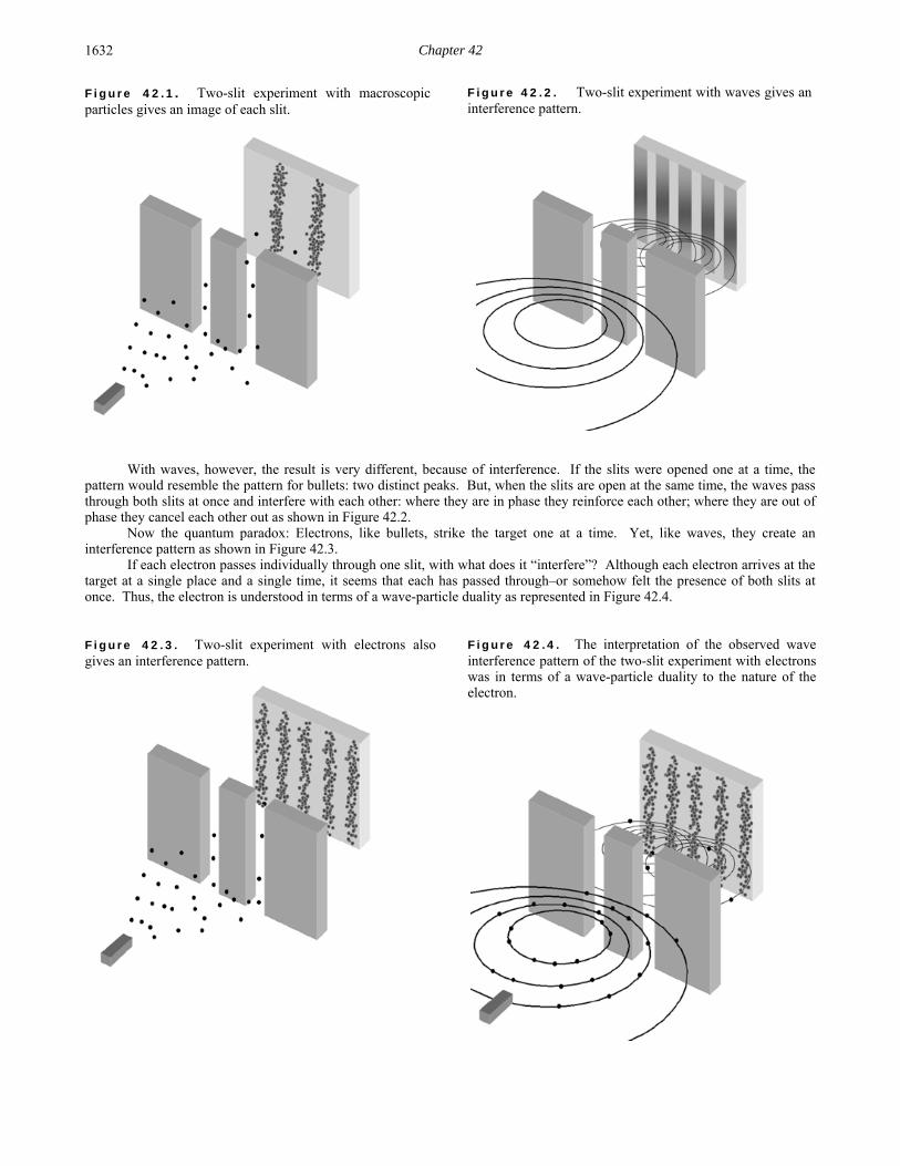
Chapter 42 1632
Figure 42.1. Two-slit experiment with macroscopic particles gives an image of each slit.
With waves, however, the result is very different, because of interference. If the slits were opened one at a time, the
pattern would resemble the pattern for bullets: two distinct peaks. But, when the slits are open at the same time, the waves pass through both slits at once and interfere with each other: where they are in phase they reinforce each other; where they are out of phase they cancel each other out as shown in Figure 42.2.
Now the quantum paradox: Electrons, like bullets, strike the target one at a time. Yet, like waves, they create an interference pattern as shown in Figure 42.3.
If each electron passes individually through one slit, with what does it “interfere”? Although each electron arrives at the target at a single place and a single time, it seems that each has passed through–or somehow felt the presence of both slits at once. Thus, the electron is understood in terms of a wave-particle duality as represented in Figure 42.4. Figure 42.3. Two-slit experiment with electrons also gives an interference pattern.
Figure 42.2. Two-slit experiment with waves gives an interference pattern.
Figure 42.4. The interpretation of the observed wave interference pattern of the two-slit experiment with electrons was in terms of a wave-particle duality to the nature of the electron.

Retrospect: Wave-Particle Duality 1633
The mistake in the direction of the development of the theory of light and the atom occurred when theoreticians concluded: The laws of physics that are valid in the macroworld do not hold true in the microworld of the atom. In contrast, as shown in previous chapters classical physics was applied correctly to solve the structures of the electron and photon demonstrating that the laws of physics that are valid in the macroworld do hold true in the microworld of the atom. The predictions, which arise from the equations of light and atomic particles, are completely consistent with observation, including the wave-particle duality of light and atomic particles as shown explicitly in the Classical Photon and Electron Scattering section. Furthermore, the quantization of atomic energy levels arises classically without invoking new physics. Continuous motion such as electronic transitions between quantized states and translational motion restores continuity and causality with the continuous nature of spacetime itself restored consistent with first principles and observation. The postulates and mathematical constructs of quantum mechanics are erroneous. Physical laws apply to the atomic scale in refutation to quantum mechanics.
Maxwell unified electricity and magnetism by proposing the existence of electromagnetic waves that travel at the velocity c . In 1888, Hertz showed that electromagnetic waves exist and behave exactly as Maxwell had predicted—they had electric and magnetic components, and they could be reflected, refracted, and diffracted. Toward the end of the 19th century, many physicists believed that all of the principles of physics had been discovered. The accepted principles, now called classical physics, included laws relating to Newton’s mechanics, Gibbs’ thermodynamics, LaGrange’s and Hamilton’s elasticity and hydrodynamics, Maxwell-Boltzmann molecular statistics, and Maxwell’s Equations. However, the discovery that the intensity of blackbody radiation goes to zero, rather than infinity as predicted by the prevailing laws of electromagnetism, led theoreticians to question the validity of Maxwell’s Equations on the atomic scale. In 1900, Planck made the revolutionary assumption that energy levels were quantized, and that atoms of the blackbody could emit light energy only in amounts given by h , where is the radiation’s frequency and h is a proportionality constant (now called Planck’s constant). This assumption does not conflict with the notion that light is a wave. However, Hertz’s experiments with light further revealed that photoelectrons were emitted from illuminated metals, and the photoelectron energy increases with the frequency of incident light and not its intensity. Einstein explained this photoelectron effect by proposing that light of a given frequency is composed of individual photons whose energy is proportional to that frequency according to Planck’s relationship1. Einstein’s proposal that light has a particle nature in that it travels through space as distinct photons2 is opposed to the wave view whereby light waves spread out from a source, and the energy is spread continuously throughout the wave pattern. Thus, light has since been regarded as both a wave and a particle which exhibits one feature or the other during observation but never both simultaneously. Early 20th century theoreticians proclaimed that light has a wave-particle duality that was unlike anything in our common everyday experience [3].
A similar course arose in the development of the model of the atom. J. J. Balmer showed, in 1885, that the frequencies for some of the lines observed in the emission spectrum of atomic hydrogen could be expressed with a completely empirical relationship. This approach was later extended by J. R. Rydberg, who showed that all of the spectral lines of atomic hydrogen were given by the equation:
2 2
1 1
f i
Rn n
(42.1)
where 110,967,758 R m , 1, 2,3,...fn , 2,3,4,...in , and i fn n . Niels Bohr, in 1913, developed a theory for atomic
hydrogen based on an unprecedented postulate of stable circular orbits that do not radiate. Although no explanation was offered for the existence of stability for these orbits, the results gave energy levels in agreement with Rydberg’s equation. Bohr’s theory was a straightforward application of Newton’s laws of motion and Coulomb’s law of electric force—both pillars of classical physics and is in accord with the experimental observation that atoms are stable. However, it is not in accord with electromagnetic theory—another pillar of classical physics, which predicts that accelerated charges radiate energy in the form of electromagnetic waves. An electron pursuing a curved path is accelerated and therefore should continuously lose energy, spiraling into the nucleus in a fraction of a second. The predictions of electromagnetic theory have always agreed with experiment, yet atoms do not collapse. To the early 20th century theoreticians, this contradiction could mean only one thing: The laws of physics that are valid in the macroworld do not hold true in the microworld of the atom. In 1923, de Broglie suggested
that the motion of an electron has a wave aspect—h
p . This concept seemed unlikely according to the familiar properties of
electrons such as charge, mass and adherence to the laws of particle mechanics. But, the wave nature of the electron was confirmed by Davisson and Germer in 1927 by observing diffraction effects when electrons were reflected from metals. Schrödinger reasoned that if electrons have wave properties, there must be a wave equation that governs their motion. And in 1926, he proposed the Schrödinger equation, H E , where is the wave function, H is the wave operator, and E is the energy of the wave. This equation, and its associated postulates, is now the basis of quantum mechanics, and it is the basis for the worldview that the atomic realm including the electron and photon cannot be described in terms of “pure” wave and “pure” particle but in terms of a wave-particle duality. The wave-particle duality based on the fundamental principle that physics on an atomic scale is very different from physics on a macroscopic scale is central to present day atomic theory [4]. 1 In 1900, Planck made the revolutionary assumption that energy levels were quantized, and that atoms of the blackbody could emit light energy only in amounts given by h , where is the radiation’s frequency and h is a proportionality constant (now called Planck’s constant). This assumption also led to our understanding of the photoelectric effect and ultimately to the concept of light as a particle called a photon. 2 This view was first proposed by Newton. Einstein was the founder of the erroneous wave-particle duality concept that’s the source of “weirdness” in quantum mechanics.

Chapter 42 1634
The hydrogen atom is the only real problem for which the Schrödinger equation can be solved without approximations; however, it only provides three quantum numbers–not four. Nevertheless, the application of the Schrödinger equation to real problems has provided useful approximations for physicists and chemists. Schrödinger interpreted *( ) ( )e x x as the charge-density or the amount of charge between x and x dx ( * is the complex conjugate of ) wherein he pictured the electron to be spread over large regions of space. Three years after Schrödinger’s interpretation, Max Born, who was working with scattering theory, found that this interpretation led to inconsistencies and he replaced the Schrödinger interpretation with the probability of finding the electron between x and x dx as:
( ) *( )x x dx (42.2)
Born’s interpretation is generally accepted. Nonetheless, interpretation of the wave function is a never-ending source of confusion and conflict. Many scientists have solved this problem by conveniently adopting the Schrödinger interpretation for some problems and the Born interpretation for others. This duality allows the electron to be everywhere at one time—yet have no volume. Alternatively, the electron can be viewed as a discrete particle that moves here and there (from 0r to r ), and
* gives the time average of this motion. According to the quantum mechanical view, a moving particle is regarded as a wave group. To regard a moving particle
as a wave group implies that there are fundamental limits to the accuracy with which such “particle” properties as position and momentum can be measured. Quantum mechanics predicts that the particle may be located anywhere within its wave group
with a probability 2 . An isolated wave group is the result of superposing an infinite number of waves with different
wavelengths. The narrower the wave group is, the greater range of wavelengths involved. A narrow de Broglie wave group thus means a well-defined position ( x smaller) but a poorly defined wavelength and a large uncertainty p in the momentum of the particle the group represents. A wide wave group means a more precise momentum but a less precise position. The infamous Heisenberg Uncertainty Principle is a formal statement of the standard deviations of properties implicit in the probability model of: fundamental particles.
2
x p
(42.3)
According to the standard interpretation of quantum mechanics, the act of measuring the position or momentum of a quantum mechanical entity collapses the wave-particle duality because the principle forbids both quantities to be simultaneously known with precision. (The Resonant Line Shape and Lamb Shift section discusses the erroneous nature of the Uncertainty Principle.) THE WAVE-PARTICLE DUALITY IS NOT DUE TO THE UNCERTAINTY PRINCIPLE Quantum entities can behave like particles or waves, depending on how they are observed. They can be diffracted and produce interference patterns (wave behavior) when they are allowed to take different paths from some source to a detector—in the usual example, electrons or photons go through two slits and form an interference pattern on the screen behind. On the other hand, with an appropriate detector put along one of the paths (at a slit, say), the quantum entities can be detected at a particular place and time, as if they are point-like particles. But any attempt to determine which path a quantum object takes destroys the interference pattern. Richard Feynman described this as the central mystery of quantum physics.
Bohr called this vague principle “complementarity,” and explained it in terms of the uncertainty principle, put forward by Werner Heisenberg, his postdoc at the time. In an attempt to persuade Einstein that wave-particle duality is an essential part of quantum mechanics, Bohr constructed models of quantum measurements that showed the futility of trying to determine which path was taken by a quantum object in an interference experiment. As soon as enough information is acquired for this determination, the quantum interferences must vanish, said Bohr, because any act of observing will impart uncontrollable momentum kicks to the quantum object. This is quantified by Heisenberg’s uncertainty principle, which relates uncertainty in positional information to uncertainty in momentum—when the position of an entity is constrained, the momentum must be randomized to a certain degree.
More than 60 years after the famous debate between Niels Bohr and Albert Einstein on the nature of quantum reality, a question central to their debate—the nature of quantum interference—has resurfaced. The usual textbook explanation of wave-particle duality in terms of unavoidable “measurement disturbances” is experimentally proven incorrect by an experiment reported in the September 3, 1998 issue of Nature [5] by Durr, Nonn, and Rempe. Durr, Nonn, and Rempe report on the interference fringes produced when a beam of cold atoms is diffracted by standing waves of light. Their interferometer displayed fringes of high contrast—but when they manipulated the electronic state within the atoms with a microwave field according to which path was taken, the fringes disappeared entirely. The interferometer produced a spatial distribution of electronic populations that were observed via fluorescence. The microwave field canceled the spatial distribution of electronic populations. The key to this new experiment was that although the interferences are destroyed, the initially imposed atomic momentum distribution left an envelope pattern (in which the fringes used to reside) at the detector. A careful analysis of the pattern demonstrated that it had not been measurably distorted by a momentum kick of the type invoked by Bohr, and therefore that any locally realistic momentum kicks imparted by the manipulation of the internal atomic state according to the particular path of the atom are too small to be responsible for destroying interference.
Durr et al. conclude that the “Heisenberg Uncertainty relationship has nothing to do with wave-particle duality” and further conclude that the phenomenon is based on entanglement and correlation. Their interpretation of the principles

Retrospect: Wave-Particle Duality 1635
of the experiment is that directional information is encoded by manipulating the internal state of an atom with a microwave field, which entangles the atom’s momentum with its internal electronic state. Like all such entangled states, the constituent parts lose their separate identity. But the attachment of a distinguishable electronic label to each path means that the total electronic-plus-path wavefunction along one path becomes orthogonal to that along the other, and so the paths can’t interfere. By encoding information as to which path is taken within the atoms, the fringes disappear entirely. The internal labeling of paths does not even need to be read out to destroy the interferences: all you need is the option of being able to read it out.
According to Durr et al., the mere existence of information about an entity’s path causes its wave nature to disappear. But, correlations are observations about relationships between quantities and do not cause physical processes to occur. The existence of information about an entity’s path is a consequence of the manipulation of the momentum states of the atoms which resulted in cancellation of the interference pattern. It was not the cause of the cancellation. The cancellation is predicted by classical atomic theory.
The explanation for the loss of interference in which-way experiments that endured and is present in essentially all quantum physics textbooks is that based on Heisenberg’s position-momentum uncertainty relation. This has been illustrated in famous gedanken experiments like Einstein’s recoiling slit [6] or Feynman’s light microscope [7]. In the light microscope, electrons are illuminated with light immediately after they have passed through a double slit with slit separation d . A scattered photon localizes the electron with a position uncertainty of the order of the light wavelength, lightz . Owing to Heisenberg’s
position-momentum uncertainty relation, this localization must produce a momentum uncertainty of the order of /z lightp h .
This momentum uncertainty arises from the momentum kick transferred by the scattered photon. For light d , which-way
information is obtained, but the momentum kick is so large that it completely washes out the spatial interference pattern. The issue of whether momentum kicks are necessary to explain the two-slit experiment is revisited. Obviously,
momentum is involved, because a diffraction pattern is a map of the momentum distribution in the experiment. But how is it involved? Is it everything, as Bohr would have claimed?
This is the question addressed by Durr et al. [5] who report on a which-way experiment with an atom interferometer wherein an incoming beam of atoms passes through two separated standing wave light beams. The detuning of the light frequency from the atomic resonance, light atom , is large so that spontaneous emission can be neglected. The light fields
each create a conservative potential U for the atoms, the so-called light shift, with /U I , where I is the light intensity. In a standing wave, the light intensity is a function of position where,
20 cos lightI z I k z (42.4)
where lightk is the wavevector of the light. Hence the light shift potential takes the form of:
20 cos lightU z U k z (42.5)
with 0 0 /U I .
The atoms are Bragg-reflected from this periodic potential, if they enter the standing light wave at a Bragg angle. This process is similar to Bragg reflection of X-rays from the periodic structure of a solid-state crystal, but with the role of matter and light exchanged. The light creates the periodic structure, from which the matter wave is reflected.
The scheme of the interferometer is shown in Figure 42.5. The standing light wave splits the incoming atomic beam A into two beams, a transmitted beam C and a first-order Bragg-reflected beam B. The angle between the beams B and C corresponds to a momentum transfer of exactly 2 lightk as determined by the spatial period of ( )U z . By varying the light
intensity, the fraction of reflected atoms can be adjusted to any arbitrary value. Durr et al. tune the reflectivity of the beam splitter to about 50%.

Chapter 42 1636
Figure 42.5. Scheme of the atom interferometer. The incoming atomic beam A is split into two beams: beam C is transmitted and beam B is Bragg-reflected from a standing light wave. The beams are not exactly vertical because a Bragg condition must be fulfilled. After free propagation for a time sept , the beams are displaced by a distance d . Then the beams are
split again with a second standing light wave. In the far field, a spatial interference pattern is observed.
After switching off the first standing light wave, the two beams are allowed to propagate freely for a time interval sept .
During this time, beam B moves a horizontal distance / 2d to the left, and beam C moves / 2d to the right. The longitudinal velocities (direction normal to the standing light wave of Figure 42.5) of the two beams are not affected by the light field. Then a second standing light wave is switched on, which also serves as a 50% beam splitter. Now two atomic beams D and E are traveling to the left, while beams F and G are traveling to the right. In the far field, each pair of overlapping beams produces a spatial interference pattern. The fringe period is the same as in a double-slit experiment with slit separation d as given in Two-Beam Interference section. The intensity is given by Eq. (8.23) :
2 2 2 22 x 2 x(x) 16 sinc cos
a dI a C
f f
(42.6)
From Eq. (42.6), it is clear that the resulting pattern has the appearance of 2cosine fringes of period /f d with an envelope
2sinc 2 x /a f where f is the focal length and a is the slit width. In the present case, the envelope of the fringe pattern is
given by the collimation properties of the initial atomic beam A. Note that Eq. (42.6) corresponds to an amplitude transmission of a plane wave. The bound unpaired electron of each 85Rb atom behaves as a plane wave of wavelength /h p as shown in the Free Electron section. The relevant wavelength of Eq. (42.6) is the de Broglie wavelength associated with the momentum of the atoms (Eq. (1.38)) which is transferred to the electrons through atomic interactions.
The atomic position distribution is observed by exciting atoms with a resonant laser and detecting the fluorescence photons. The observed far-field position distribution is a picture of the atomic transverse momentum distribution after the interaction. The pattern is given by Eq. (42.6). The pattern may be altered by application of microwave pulses which transfer momentum to the electrons of the 85Rb atoms which add vectorially to that transferred from the interactions with the standing light field and atomic interactions.
Microwave pulses are now added to manipulate the two internal electronic states of the atom according to whether it moved along pathway B or C. A simplified level scheme of 85Rb is shown in Figure 42.6. The manipulation of internal states by two microwave fields which each apply a / 2 pulse is shown in Figure 42.7. Rabi oscillations between states 2 and 3
can be induced by applying a microwave field of about 3 GHz. To describe the manipulation of the two internal electronic states of the atom, we first investigate the properties of a single Bragg beam splitter.

Retrospect: Wave-Particle Duality 1637
Figure 42.6. Simplified level scheme of 85Rb . The
excited state 23/25 P is labeled e . The ground state
21/25 P is split into two hyperfine states with total angular
momentum 2F and 3F , which are labeled 2 and 3 ,
respectively. The standing light wave has angular frequency
light .
The frequency of the standing light wave, light is tuned halfway between the 2 e and 3 e transitions. Hence
the detunings from these transitions, 2e , and 3e , have the same absolute value but opposite sign. The reflectivity of the beam
splitter, that is, the probability of reflecting an atom, depends on 0Braggt X U , and it is independent of the internal state.
However, the amplitude of the wavefunction experiences a phase shift which depends on the internal atomic state. A simple analogy for this phase shift can be found in light optics: a light wave reflected from an optically thicker medium experiences a phase shift of , while reflection from an optical thinner medium or transmission into an arbitrary medium does not cause any phase shift. This argument also applies in atomic optics: in the present experiment, an atom in 2 sees a negative
light shift potential (because 2 0e ), corresponding to an optically thicker medium, while an atom in 3 sees a positive
potential (because 3 0e ), corresponding to an optically thinner medium. Hence an atom will experience a phase shift only
if it is reflected in 2 .
This phase shift can be converted into a population difference between the hyperfine levels. For that purpose, two microwave / 2 pulses resonant with the hyperfine transition are applied. They form a Ramsey scheme as shown in Figure 42.7. The atom is initially prepared in state 2 . Then a / 2 microwave pulse is applied, converting the beam into an equal
mixture of internal states of 2 3 . After this, each atom interacts with the standing light wave. As explained above, each
atom will experience a phase shift only if it is reflected and in state 2 . Thus the internal state of the reflected beam is
changed to an equal mixture of internal states of 3 2 , while the internal state of the transmitted beam is not affected. As a
result, the momentum of each atom is a superposition of the internal and external degree of freedom of the atom which is specific to the path. The state vector of the system becomes:
3 2 3 2B C (42.7)
where B and C describe the center-of-mass motion for the reflected and transmitted beams (see Figure 42.5),
respectively. The second microwave pulse action on both beams (the transmitted and the reflected), converts the internal state of the transmitted beam to state 3 , while the reflected beam is converted to state - 2 . Thus, the state vector after the pulse
sequence shown in Figure 42.7 becomes: 2 3B C (42.8)
Eq. (42.8) shows that the internal state is correlated with the way taken by the atom. The which-way information can be read out later by performing a measurement of the internal atomic state. The result of this measurement reveals which way the atom took: if the internal state is found to be 2 , the atom moved along beam B, otherwise it moved along beam C.
After considering a single beam splitter, now consider the complete interferometer. Sandwiching the first Bragg beam splitter between two / 2 microwave pulses produces a reflected and transmitted beam each of a single internal atomic state, as described above. We note that the second Bragg beam splitter does not change the internal state. No fringes are
Figure 42.7. Scheme of the manipulation of internal states of 85Rb by two microwave fields which each apply a
/ 2 pulse. The standing light wave with angular frequency
light induces a light shift for both ground states, which is
given as a function of position. The beam splitter produces a phase shift that depends on the internal and external degree of freedom. A Ramsey scheme, consisting of two microwave
/ 2 pulses, converts this phase shift into a population difference.

Chapter 42 1638
experimentally observed in this case. The data is recorded with the same parameters with the only difference being that two microwave pulses are added to produce a single internal atomic state according to the particular path of the atom. Atoms in both hyperfine states are detected. The interference pattern is also not observed when only atoms in state 2 or only atoms in state
3 are detected. Of course, the absolute size of the signal is reduced by a factor of two in these cases. The key to this new
experiment is that although the interferences are destroyed, the initially imposed atomic momentum distribution leaves an envelope pattern (in which the fringes used to reside) at the detector. A careful analysis of the pattern finds that it has not been measurably distorted by a momentum kick of the type invoked by Bohr, and therefore that any locally realistic momentum kicks imparted by the manipulation of the internal atomic state according to the particular path of the atom are too small to be responsible for destroying interference.
In order to investigate why the interference is lost, we consider the state vector for the interaction sequence used which causes the disappearance of the fringes. The state vector after the interaction with the first beam splitter sandwiched between the two microwave pulses is given by Eq. (42.8). The second beam splitter transforms this state vector into a left peak and a right peak given by:
2 3left D E (42.9)
and
2 3right F G (42.10)
where the sign of F is positive due to the phase shift during the reflection from the second beam splitter. Each peak is a
superposition of atoms which follow separate paths and comprise atoms of a single internal state. In each case atoms which interfere have internal states which are orthogonal; thus, in the far field, the atomic position distribution under each peak of the envelope is given by the superposition of two single slit patterns rather than the double slit pattern in the absence of the application of the / 2 microwave pulses. In the far field, the amplitude of the atomic position distribution under each peak of the envelope (x) is the sum of the independent Fraunhofer planes and the intensity of the atomic position distribution under
each peak of the envelope 2 (x) is given by:
22 2 x(x) 2 sinc
f
kaaC
(42.11)
where f is the focal length and a is the slit width. In the present case, the envelope of the fringe pattern is given by the collimation properties of the initial atomic beam A.
A dramatic change in the spatial momentum distribution occurs when adding the microwave fields to the interferometer that manifests itself as loss of interference; even though, the microwave itself does not transfer enough momentum to the atom to wash out the fringes according to the Heisenberg Uncertainty Principle. The addition of the microwave fields modifies the probability for momentum transfer by the light fields. This modification of the momentum transfer probability is due to the manipulation of the internal atomic state according to the particular path of the atom. The disappearance of interference is explained by classical physics. In addition to the invalidation of the HUP as the basis of the wave particle duality, the other aspect of the HUP, the measurement-disturbance relationship of the HUP, has been tested for the first time and experimentally disproved [L. A. Rozema, A. Darabi, D. H. Mahler, A. Hayat, Y. Soudagar, A. M. Steinberg, “Violation of Heisenberg’s Measurement-Disturbance Relationship by Weak Measurements,” Phys. Rev. Lett., 109 (2012), 100404.]. INCONSISTENCIES OF QUANTUM MECHANICS Quantum mechanics failed to predict the results of the Stern-Gerlach experiment which indicated the need for an additional quantum number. Quantum electrodynamics was proposed by Dirac in 1926 to provide a generalization of quantum mechanics for high energies in conformity with the theory of Special Relativity and to provide a consistent treatment of the interaction of matter with radiation. From Weisskopf [8], “Dirac’s quantum electrodynamics gave a more consistent derivation of the results of the correspondence principle, but it also brought about a number of new and serious difficulties.” Quantum electrodynamics; (1) does not explain nonradiation of bound electrons; (2) contains an internal inconsistency with Special Relativity regarding the classical electron radius–the electron mass corresponding to its electric energy is infinite; (3) it admits solutions of negative rest mass and negative kinetic energy; (4) the interaction of the electron with the predicted zero-point field fluctuations leads to infinite kinetic energy and infinite electron mass; (5) Dirac used the unacceptable states of negative mass for the description of the vacuum; yet, infinities still arise. In 1947, Lamb discovered a 1000 MHz shift between the 2
1/2S state and the 21/2P state of
the hydrogen atom. This so called Lamb Shift marked the beginning of modern quantum electrodynamics. In the words of Dirac [9], “No progress was made for 20 years. Then a development came initiated by Lamb’s discovery and explanation of the Lamb Shift, which fundamentally changed the character of theoretical physics. It involved setting up rules for discarding ...infinities...” Renormalization is presently believed to be required of any fundamental theory of physics [10]. However, dissatisfaction with renormalization has been expressed at various times by many physicists including Dirac [11]. who felt that, “This is just not sensible mathematics. Sensible mathematics involves neglecting a quantity when it turns out to be small—not neglecting it just because it is infinitely great and you do not want it!”
Modern quantum mechanics has encountered several obstacles that have proved insurmountable as pointed out previously in the General Considerations section and the Classical Electron Radius section. It is not based on physical laws, and
Retrospect: Wave-Particle Duality 1639
is not predictive as discussed previously [8, 12–24]. SQM has never dealt with the nature or structure of fundamental particles. They are treated as zero-dimensional points that occupy no volume and are everywhere at once. This view is impossible since occupying no volume would preclude their existence; the inherent infinities are not observed nor are they possible, and the possibility of a particle being everywhere at once violates all physical laws including conservation of energy and causality. Furthermore, it leads to certain philosophical interpretations [25] which are not sensible. Some conjure up multitudes of Universes including “mind” Universes; others require belief in a logic that allows two contradictory statements to be true. The question addressed is whether the Universe is determined or influenced by the possibility of our being conscious of it. The meaning of quantum mechanics is debated, but the Copenhagen interpretation is predominant. Its asserts that “what we observe is all we can know; any speculation about what a photon, an atom or even a SQUID (Superconducting Quantum Interference Device) really is or what it is doing when we are not looking is just that speculation [26].” According to this interpretation every observable exists in a state of superposition of possible states, and observation or the potential for knowledge causes the wavefunction corresponding to the possibilities to collapse into a definite one. As shown by Platt [27] in the case of the Stern-Gerlach experiment, “the postulate of quantum measurement [which] asserts that the process of measuring an observable forces the state vector of the system into an eigenvector of that observable, and the value measured will be the eigenvalue of that eigenvector.”
According to the Zeno no-go theorem which is a consequence of the postulate of quantum measurement, observation of an atom collapses its state into a definite; thus, transitions cannot occur under continuous observation. Recently, it has become possible to test this postulate via an experiment involving transitions of a single atom, and the results are inconsistent with the predictions. Quoting from the caption of Figure 10 of the article, by Dehmelt [28],
“Shelving” the Ba+ optical electron in the metastable D level. Illuminating the ion with a laser tuned close to its resonance line produces strong resonance fluorescence and an easily detectable photon count of 1600 photons/sec. When later an auxiliary, weak Ba+ spectral lamp is turned on, the ion is randomly transported into the metastable 5/2D
level for 30-s lifetime and becomes invisible. After dwelling in this shelving level for 30 s on average, it drops down to the S ground state spontaneously and becomes visible again. This cycle repeats randomly. According to the Zeno no-go theorem, no quantum jumps should occur under continuous observation.
The Copenhagen interpretation equally applies to witnessing the presence of the moon. According to quantum
mechanics the moon is not there until it is observed. Since the act of measuring is relative to each individual observer and it is “entangled” with each observer, the “collapse” must result in different realities for different observers of presumably the same object. Thus, Man’s consciousness has a special position in the most popular interpretation of quantum mechanics as the engine of reality and individualism results in the conjuring up of multitudes of Universes including parallel “mind” Universes [25].
Of course this is nonsense and is a consequence of the mistake of originally postulating that fundamental particles are probability waves rather than real. Furthermore, the brain obeys the same physical laws as the rest of the matter of the Universe. Sodium, potassium, and chloride ions in the brain are obtained from the ambient environment are constantly being interchanged with that environment. The same rules apply irrespective of where that matter is found. In fact, the phenomena of the ability of the brain to reason and to produce a state called consciousness has nothing to do with god-like properties unique to humans that are deeply seated in quantum folklore. Rather, it can be traced to simple properties of excitable neurons, their organization, and simple thermodynamic principles exploited by biological systems to more or lesser extents over millions of years of evolution.
At the most fundamental level, a conscious being is made of energy, quarks, gluons, electrons, atoms, molecules, etc. that originate from and are part of the Universe. For example, the elements of humans other than hydrogen originate in stars. Therefore, in broader terms, the physics of the Universe dynamically gives rise to a conscious being, and it is implicit that the Universe is aware of itself. Then, distinctions exist between animate beings and inanimate objects that must follow first principles. Consciousness, the ability of a chemical reaction to be aware of itself arises from the relationship of energy changes to entropy. If the brain chemistry of conscious beings behaved as typical chemical reactions following an arrow of time according to typical enthalpy and concomitant entropy changes, then any information stored and processed by the brain would decrease over time, and consciousness would not be possible. The brain chemistry comprising ion channel conductance changes, ion flows, ion pump activity, metabolic reactions, etc., comprise an energy state in opposition to the thermodynamic arrow of time. Living beings produce negative entropy at the expense of their surroundings. In other words, consciousness is achieved against the arrow of time discussed in the Arrow of Time and Entropy section by increasing the entropy of the surroundings to offset its relatively low entropic state. Consciousness is shaped by and requires the environment with which the brain interacts and depends for a source of energy and materials to maintain the local-temporal high entropic state relative to its surroundings.
A previous publication [29-30] showed that the brain is governed by the entropy principle of thermodynamics whereby the wet-chemistry-based system comprising excitable neurons arranged in a spatial-temporal hierarchy of ensembles in a dynamical state of activation and connectivity dependent on present and past activation rates, influenced by past and present input from the environment, achieves a state representative of a predominant configuration, the most probable state in time. The brain must be active continuously as a predominant configuration. This time-dependent state based on the second law of thermodynamics and comprising representations of aspects of the physical Universe is the basis of consciousness.
In addition to exploiting the second law of thermodynamics with the formation of a predominant configuration, the brain has evolved to exploit several fundamental signal processing principles to achieve consciousness. For example, the brain
Chapter 42 1640
functions as an analog Fourier processor which transduces and processes information representative of physical characteristics or representations of physical characteristics as Fourier series in Fourier space. The brain also exploits time using spatial segregation of stored information as a means to encode context of the physical characteristics of the information. Specific time delays arising from the spatial separation of propagating signals correspond to modulation of the Fourier series at corresponding frequencies to encode the context. The brain associates information by exploiting the principle that cascaded stages such as association neurons give rise to delayed Gaussian filters. And, filtered signals may be associated based on the physics of energy exchange between two or more harmonic states. Given the evolutionary ascension of multicellular organisms each producing negative entropic states and having specialized cells with excitable membranes, the progress to consciousness and intelligence was inevitable. The first-principles-based theory of the signal processing mechanism of the brain and the origin of consciousness was published previously with a means to computer-simulate these phenomena [29-30].
Specifically, a method and system for pattern recognition and processing involving processing information in Fourier space was reported [29-30]. The theoretical results given previously are that (1) action potentials carry information with digital and analog aspects that allows the brain to operate as a Fourier processor in Fourier space with encoding of context in the structure of transducers mapping one-to-one with corresponding structural elements of the memory, (2) an ensemble of interlinked neurons can filter information as delayed Gaussian filters, (3) the neuronal ensembles propagating cascaded action potentials may couple with Poison probability to form associations of information encoded in the action potentials, (4) ensembles of neurons as delayed Gaussian filters may order format information by forming associations of the corresponding filtered action potentials with memory elements, and (5) a predominant configuration of activation may arise that is analogous to that of interacting quantum levels with partition of energy as given by statistical thermodynamics. These aspects are modeled such that a simulation may be programmable on digital processing systems.
This novel approach anticipates the signal processing action of an ensemble of neurons as a unit and intends to simulate aspects of brain that give rise to capabilities such as intelligence, pattern recognition, reasoning, and ultimately consciousness that have not been reproduced with past approaches such as neural networks that are based on individual simulated “neuronal units.” Information representative of physical characteristics or representations of physical characteristics is transformed into a Fourier series in Fourier space within an input context of the physical characteristics that is encoded in time as delays corresponding to modulation of the Fourier series at corresponding frequencies. Associations are formed between Fourier series by filtering the Fourier series and by using a spectral similarity between the filtered Fourier series to determine the association based on Poissonian probability. The associated Fourier series are added to form strings of Fourier series. Each string is ordered by filtering it with multiple selected filters to form multiple time order formatted subset Fourier series, and by establishing the order through associations with one or more initially ordered strings to form an ordered string. Associations are formed between the ordered strings to form complex ordered strings that relate similar items of interest. The components of the system based on the algorithm are active based on probability using weighting factors based on activation rates. The probabilistic activation, based on past activation rates, gives rise to a system state akin to a time-dependent predominate configuration of statistical thermodynamics that can be associated with consciousness. THE ASPECT EXPERIMENT—NO SPOOKY ACTIONS AT A DISTANCE In addition to the interpretation that photons, electrons, neutrons, and even human beings [25] have no definite form until they are measured, a more disturbing interpretation of quantum mechanics is that a measurement of a quantum entity can instantaneously influence another light years away. Einstein argued that a probabilistic versus deterministic nature of atomic particles leads to disagreement with Special Relativity. In fact, the nonlocality result of the Copenhagen interpretation violates causality. As a consequence of the indefinite nature of the Universe according to quantum mechanics and the implied Uncertainty Principle, Einstein, Podolsky, and Rosen (EPR) in a classic paper [31] presented a paradox which led them to infer that quantum mechanics is not a complete theory. They concluded that the quantum-mechanical description of a physical system should be supplemented by postulating the existence of “hidden variables,” the specification of which would predetermine the result of measuring any observable of the system. They believed the predictions of quantum mechanics to be correct, but only as consequences of statistical distribution of the hidden variables. But, Bell [32] showed that in a Gedanken experiment of Bohm [34] (a variant of that of EPR) no local hidden-variable theory can reproduce all of the statistical predictions of quantum mechanics. Thus, a paradox arises from Einstein’s conviction that quantum-mechanical predictions concerning spatially separated systems are incompatible with his condition for locality unless hidden variables exist. Bell’s theorem provides a decisive test of the family of local hidden-variable theories (LHVT). In a classic experiment involving measurement of coincident photons at spatially separated detectors, Aspect [34] showed that local hidden-variable theories are inconsistent with the experimental results. Although Aspect’s results are touted as a triumph of the predictions of quantum mechanics, the correct coincidence rate of detection of photons emitted from a doubly excited state of calcium requires that the z component of the angular momentum is conserved on a photon pair basis. As a consequence, a paradox arises between the deterministic conservation of angular momentum and the Uncertainty Principle. The prediction derived from the quantum nature of the electromagnetic fields for a single photon is inconsistent with Aspect’s results, and Bell’s theorem also disproves quantum mechanics. However, the results of Aspect’s experiment are predicted by classical physics wherein locality and causality hold.
The Aspect experiment is often invoked as the proof of the quantum-mechanical nature of reality [34-42]. According to the quantum explanation of the Aspect experiment [34], the polarization of each photon of a pair is not determined until a measurement is made, and the act of measuring the polarization of one photon causes an action at a distance with regard to the measurement of the polarization of the other member of a given pair. These results are interpreted as proof of a spooky action at

Retrospect: Wave-Particle Duality 1641
a distance. Thus, information travels faster than the speed of light in violation of Special Relativity, or nonlocality and noncausality are implicit.
Bell’s theorem is a simple proof of statistical inequalities of expectation values of observables given that quantum statistics are correct and that the physical system possesses “hidden variables.” Classical physics does not possess hidden-variables. It is deterministic, and Bell’s theorem does not apply to it. The correct interpretation of the results of the Aspect experiment follows from a classical derivation from the physical nature of excited-state atoms and the corresponding emitted photons. The expectation value of the coincidence rate at separated randomly oriented polarization analyzers for pairs of photons emitted from a doubly excited state atom is derived from the equation of the photon which appears in the Equation of the Photon section.
Aspect [34] reports the measurement of polarization correlation (coincidence count rate) of visible photons ( 1 551.3 nm ; 2 422.7 nm ) emitted in a 0 1 0J J J calcium atomic cascade
2 1 1 2 10 1 04 4 4 4 p S s p P s S . The calcium atoms were selectively pumped to the upper level of the cascade from the ground
state by the two photon absorption via two lasers, a single-mode krypton ion laser and a cw single-mode Rhodamine 6G dye laser tuned to the resonance for the two photon process. The fluorescent light was collected by lenses and made incident on two detectors–one at position -z and the other at position +z relative to the emitting calcium atoms. The polarizers were independently rotated in the xy-plane, and the coincidence count rate was measured.
The equation for the transmission of an electromagnetic wave through a barrier as given in any text of classical electrodynamics such as that of Kong [43] is: zi z
T iTE e kE (42.12)
where TE is the transmitted wave, iE is the incident wave, and T is the transmission coefficient. For a wave that propagates at
an angle with respect to the z-axis, the transmitted photon is given by a sum of equations of the form of Eq. (42.12) for each vector component. Using the convention of Horne [39], the vector transmission efficiencies (coefficients) can be written in matrix form with a matrix corresponding to each linear polarizer. In a basis of linear polarizations along 1x and 1y in the
coordinates of photon 1, the most general linear polarizer with axis along 1x is described by an efficiency matrix
1
11
0
0M
m
(42.13)
where 1M is the probability of transmitting an 1x linearly polarized photon and 1
m is the probability of transmitting a 1y
linearly polarized photon (leakage). In the ideal case 1 1M and 1 0m . If the polarizer is not parallel to the 1x -axis but
rotated in the plane perpendicular to the interdetector axis by an angle 1 from 1x , and 1 is expressed in the basis of right
hand circular (RHC) and left hand circular (LHC) photon states formed from 1x and 1y , then the elementary transformations
give the elements of 1 as a function of 1 in matrix form:
1
1
21 1 1 1
1 ' '11 1 1 1 1 1
21 1
1,
2
iM m M m
M miM m
e
e
(42.14)
where '11 1 is defined as the expectation value of the transmission of the photon 1 with polarization 1 , 1 1 are
RHC and LHC, respectively, and the angle between polarizer 1 ( 1P ) and 1x is:
1 1 (42.15)
Similarly, 2 , the efficiency matrix as a function of 2 of the second polarizer ( 2P ) in the circular polarization basis of
photon 2, is
2
2
22 2 2 2
2 ' '12 2 2 2 2 2
22 2
1,
2
iM m M m
i M mM m
e
e
(42.16)
where the angle between polarizer 2 and the x-polarization of photon 2 (i.e. the angle between 2P and 2x ) is:
2 2 (42.17)
The efficiency matrix for coincidence transmission of photon 1 and photon 2 is given by the product of their independent probabilities, 1 2 . The normalized coincidence counting rate is
1 2
0
f
f
Tr pR
R Tr Ip (42.18)

Chapter 42 1642
The normalized coincidence counting rate with polarizer 2 removed, 1
0
R
R, is
1
1
0
f
f
Tr pR
R Tr Ip (42.19)
The normalized coincidence counting rate with polarizer 1 removed, 2
0
R
R, is:
2
2
0
f
f
Tr pR
R Tr Ip
(42.20)
where I is the identity matrix and fp is the probability that photon 1 and photon 2 have the same polarization and is a function
of solid angle of the projection of the propagation vector of each photon onto the z-axis. In terms of Eq. (42.12), fp
corresponds to the vector correlated electric field incident on the opposed detectors. It is given by the normalized electric field of photons of matched momentum projected onto the z-axis over the solid angle of the detectors.
The Excited States of the One-Electron Atom (Quantization) section gives the method to calculate the Einstein A coefficient in terms of the electric field based on classical electrodynamics that is applicable to each photon of the two photon
0 1 0J J J cascade of calcium. The Excited States of Helium section further applies the dependence of the
transition energy, and Jackson [44] applies the transition probability, on the integral of the product of the multipole of the photon, , ,p
l mX , and the initial, , ,il mX , and final, , ,f
l mX , states as is the case with classical electrodynamics
calculations involving antennas. The transition probability 1
is given by the power of the transition divided by the energy:
1
Re *1 2ddpower
energy
E HS
(42.21)
The distribution of multipole radiation and the multipole moments of the electron for absorption and emission are given in the Excited States of the One-Electron Atom (Quantization) section and in Jackson [44]. The electric-field amplitude of the emitted photon follows from that given in the Equation of the Photon section.
Horne postulates the emission as a plane wave which is replaced by a spherical multipole expansion. The spherical multipole expansion of a plane wave such as given in Jackson [45] is consistent with the Green Function as the function which corresponds to the superposition of an ensemble of photons given classically by Eqs. (4.18-4.23). Using classical Eqs. (2.64-2.65), the projection of the photon pair propagation vector onto the axis perpendicular to the plane of each detector gives a factor of one corresponding to the conservation of angular momentum for each photon pair times a solid angle correction. The result for the numerator of Eq. (42.18) is:
' '
1 1 2 2
' ' 1 ' 2 ' ' '1 2 1 1 2 2 1 1 2 2 1 2 1 2, , , * ,fTr p g g
(42.22)
where ' '1 2 1 2, * ,g g is a factor corresponding to the solid angle.
Eq. (42.22) is equivalent to Eq. (5.17) of Horne. To obtain this result, Horne suppressed the integration over 1d and
2d as well as the explicit dependence on the photon propagation vectors, 1k and 2k , respectively. (The integration was also
suppressed over frequency space as well as the explicit dependence on the photon propagation vectors, 1k and 2k in the case
that QED holds.) This is only valid if the z component of angular momentum is conserved on a photon by photon basis such that the polarization correlation distribution function is independent of angle. Otherwise, it cannot be removed from the integral. HORNE’S CALCULATION IS NOT CONSISTENT WITH THE QUANTUM-MECHANICAL NATURE OF THE ELECTROMAGNETIC FIELDS FOR A SINGLE PHOTON as described below.
Substitution of the Eq. (42.14) and (42.15) and the results of solid angle term of Eq. (42.22) into Eq. (42.18) gives the normalized coincidence count rate.
1 1 2 2 1 1 2 2
10
1 1cos 2
4 4M m M m M m M m
RF
R
(42.23)
where the solid angle factor, 1F , for the 0 1 0 electric dipole cascade is:
1
2 2 21 1 2 3
12
2F G G G
(42.24)
The normalized coincidence count rate with polarizer 2 removed, 1
0
R
R, is:

Retrospect: Wave-Particle Duality 1643
1 11
0
1
2 M m
R
R (42.25)
The normalized coincidence count rate with polarizer 1 removed, 2
0
R
R, is:
2 22
0
1
2 M m
R
R (42.26)
The transmittances iM and i
m of the polarizers (i=1 or 2) for light polarized parallel or perpendicular to the polarization axis
were measured by Aspect [34]:
1 1
2 2
0.971 0.005, 0.029 0.005,
0.968 0.005, 0.028 0.005
M m
M m
(42.27)
And, the solid angle factor, 1F , for the 0 1 0 electric dipole cascade which accounts for the solid angles subtended by the
collecting lenses of the Aspect experiment is: 1 2 0.984F F (42.28)
Substitution of the Eqs. (42.27) and (42.28) into Eq. (42.23) gives the normalized coincidence count rate as a function of the relative angle between the polarizers.
0
0.2490 0.2178cos 2R
R
(42.29)
ASPECT EXPERIMENTAL RESULTS ARE PREDICTED CLASSICALLY The sequence of events based on physical laws for Aspect’s measurement of the polarization correlation (coincidence count rate) of visible photons ( 1 551.3 nm ; 2 422.7 nm ) emitted in a 0 1 0J J J calcium atomic cascade
2 1 1 2 10 1 04 4 4 4 p S s p P s S is shown in Figures 42.8A-E.
The expectation value of the coincidence rate at separated randomly oriented polarization analyzers for pairs of photons emitted from a doubly-excited state atom was derived from the equation of the photon in Eqs. (42.12-42.29). Rather than a point
that obeys a probability-density wave, the photon is an extended particle with a radius given by 2
r
wherein is the
wavelength of the photon. Consequently, the photon’s electric field vector has a projection onto the axis of each rotated polarizer’s axis. Angular momentum of the doubly excited-state atom is conserved by emitting photons of the same linear polarization in opposite directions. Thus, the photon polarization is exactly correlated based on physics. Based on these
physical attributes of the emitted photons, the normalized coincidence count rate,
0
R
R
, as a function of the relative polarizer
orientation, , given by Eq. (42.29) matches with the results of Aspect [34] as shown in Figure 42.9. A computer simulation is given in Ref. [46].

Chapter 42 1644
Figure 42.8. (A) Calcium atoms were selectively pumped to the upper level of the cascade from the ground state by a two photon absorption via two lasers (blue beam). The fluorescent light was collected by lenses and made incident on two detectors (smooth plates)—one at position -z and the other at position +z relative to the emitting calcium atoms (blue sphere). The polarizers (plates with lines along each optical axis) were independently rotated in the xy-plane, and the coincidence count rate was measured (box connected to both detectors). (B) The source current of the doubly-excited state atom gives rise to electromagnetic fields that become emitted photons in opposite directions wherein the radius of each photon is given by the ratio of the speed of light to the velocity change of the excited state electron upon de-excitation. (C) The plane (green) of polarization of each photon pair is exactly correlated to conserve the angular momentum of the excited state. (D) The transmittance of each photon at each detector depends on the alignment or angle of the plane of polarization of the photons (random but matched) and the axis of each polarizer (rotated relative to each other by the experimenter). When the polarizers are parallel, the photons are both transmitted if each is sufficiently aligned with the polarizer. (E) Or, both are blocked if the transmittance is low due to a condition of crossed polarization of each photon and polarizer. Intermediate cases depend on the relative angle of each photon and its polarizer as shown in (C).

Retrospect: Wave-Particle Duality 1645
Figure 42.9 . The normalized coincidence count rate as a function of the relative polarizer orientation as given by Eqs. (42.23), (42.24), and Eq. (42.29) (solid curve) with the results of Aspect [34] (•) match. This result is based on the physical treatment of the photon as an extended particle that obeys Maxwell’s equations with conservation of angular momentum of the doubly-excited state calcium atom and the corresponding emission of two photons of the same linear polarization in opposite directions.
ASPECT EXPERIMENTAL RESULTS ARE NOT PREDICTED BY QUANTUM MECHANICS Eq. (5.17) of Horne (same as Eq. (42.22)) is the sum over the product of the transmission efficiencies of photon pairs of identical polarization at two independent detectors and a correction for the solid angle of the detectors for the photon pairs emitted from a remote isotropic source. The probability integral over momentum space was “suppressed” and set equal to one. Thus, the calculation is a deterministic equation. It does not correspond to the equation for coincident detection predicted by quantum mechanics. According to Jackson [47]:
For a multipole with a single m value, xM and yM vanish, while a comparison of (17.67) and (17.60) shows that:
zdM m dU
dr dr (17.68)
independent of r . This has the obvious quantum interpretation that the radiation from a multipole of order ( , )l m carries off m units of z component of angular momentum per photon of energy . Even with a superposition of different m values, the same interpretation of (17.67) holds, with each multipole of definite m contributing incoherently its share of the z component of angular momentum. Now, however the x and y components are in general nonvanishing, with multipoles of adjacent m values contributing in a weighed coherent sum. The behavior continued in (17.64) and exhibited explicitly in (17.65)-(17.67) is familiar in the quantum mechanics of a vector operator and its representation with respect to basis states of 2J and *zJ . The angular momentum of multipole fields affords a classical example of this behavior, with
the z component being diagonal in the ( , )l m multipole basis and the x and y components not. The characteristics of the angular momentum just presented hold true generally, even though our example (17.57) was
somewhat specialized. For a superposition of both electric and magnetic multipoles of various ( , )l m values, the angular momentum expression (16.63) is generalized to:
* *' ' ,2
,', '
' * *' ' ,
1Re ', ' , ', ' , *
8
', ' , ', ' , *
M
L X X
L X n X
E E M M l m l ml ml m
l lE M M E l m l m
da l m a l m a l m a l m d
dr k
i a l m a l m a l m a l m d
(17.69)
The first term in (17.69) is of the same form as (17.63) and represents the sum of the electric and magnetic multipoles separately. The second term is an interference between electric and magnetic multipoles. Examination of the structure of its angular integral shows that the interference is between electric and magnetic multipoles whose l values differ by unity. This is a necessary consequence of the parity properties of the multipole fields (see below). Apart from this complication
of interference, the properties of d
dr
M are as before.
The quantum-mechanical interpretation of (17.68) concerned the z component of angular momentum carried off by each

Chapter 42 1646
photon. In further analogy with quantum mechanics, we would expect the ratio of the square of the angular momentum to the square of the energy to have the value,
2 2 22
2 2 2
1qx y z q
M M M l lM
U U
(17.70)
But from (17.60) and (17.65)-(17.67), the classical result for a pure ( , )l m multipole is:
2 2 2
2 2 2
czMM m
U U (17.71)
The reason for this difference lies in the quantum nature of the electromagnetic fields for a single photon. If the z component of angular momentum of a single photon is known precisely, the uncertainty principle requires that the other components be uncertain, with mean square values such that (17.70) holds. On the other hand, for a state of the radiation field containing many photons (the classical limit) the mean square values of the transverse components of angular momentum can be made negligible compared to the square of the z component. Then the classical limit (17.71) applies. For a ( , )l m multipole field containing N photons it can be shown* that:
2
2 2 2
2 2 2
1
qM N N m Nl l m
NU N (17.72)
This contains (17.70) and (17.71) as limiting cases.
Consider the quantum nature of the electromagnetic fields for a single photon. According to Eqs. (17.70-17.72) of Jackson, photon pairs cannot have identical z components of angular momentum; therefore, each pair cannot have identical polarization. Each quantum-mechanical photon is a superposition of RHC, LHC, linear, and elliptic polarization. And, in the case of Quantum Electrodynamics (QED), each photon is also a superposition over frequency space. In the quantum-mechanical case Eq. (17.71) of Jackson applies–the z component of angular momentum is conserved on the average of many photons. Probability applies to the emission of a pair of photons of identical polarizations (the correlation of polarizations cannot be one ( , 1P A B )) as well as to the detection of the photons of equal polarizations. Furthermore, QED requires that the probability
associated with emission as well as detection applies to a distribution of photon wavelengths with expectation values of
1 551.3 nm and 2 422.7 nm . The coincidence count rate is a function of the dot product of the electric field vector of each
photon pair having correlated polarization onto the z-axis, and the probability of detection of the separate members of each pair at the separate detectors where the associated probabilities are independent. Thus, the probability of detecting a coincident event is given by the product of their independent probabilities. The quantum nature of the electromagnetic fields for a single photon requires a fp of Eq. (42.18) that includes all distributions. Thus, the coincident rate predicted by quantum mechanics is
less than the experimental rate. The extent of the error, which is a function of the relative angle of the polarizers, is given by Bell’s theorem. BELL’S THEOREM TEST OF LOCAL HIDDEN VARIABLE THEORIES (LHVT) AND QUANTUM MECHANICS Using the convention of Clauser and Horne [37, 39], consider an ensemble of correlated pairs of photons emitted from the 0 1 0 cascade of excited state calcium atoms each moving so that one enters polarizer 1 ( 1P ) and the other polarizer 2 ( 2P ),
where 1 and 2 are adjustable angles of polarizer 1 and 2. In each polarizer a photon is recorded as +1 corresponding to RHC
and LHC polarized, respectively. Let the results of these selections be represented by A a and B b , each of which equals +1
according as the RHC or LHC is recorded. Suppose now that a statistical correlation of A a and B b is due to information carried by and localized within each
photon, and that at some time in the past the photons constituting one pair were in contact and in communication regarding this information. The information is quantum mechanical or is part of the content of a set of hidden variables, denoted collectively by . The results of the two polarization outcomes are then to be functions ,A a and ,B b . Locality reasonably requires
,A a to be independent of the parameter b and ,B b to be likewise independent of a , since the two outcomes may occur
at an arbitrarily great distance from each other. Finally, since the pair of photons is generally emitted by a source in a manner physically independent of the adjustable parameters a and b , we assume that the normalized probability distribution
characterizing the ensemble is independent of a and b . The requirement that the expectation value of a and b is equal to one ( , 1E a b ) (on the average, the polarization of photons incident on each polarizer are equal) implies , ,B a A a .
Defining the correlation function ( , ) ( , ) ( , ( )P a b A a B b d where is the total space, generalization of Bell’s
theorem gives

Retrospect: Wave-Particle Duality 1647
, , ( , ) ( , ( , ) ( , ( )
( , ) ( , 1 ( , ) ( , ( )
1 ( , ) ( , ( )
1 ( , ) ( , ( )
P a b P a c A a B b A a B c d
A a B b B b B c d
B b B c d
B b B c d
(42.30)
In the case of the 0 1 0 cascade, the coincidence count rate, ,R a b , replaces the correlation function, ,P a b , of the
generalization of Bell’s theorem which then yields the following inequalities [34]:
1 2
0
, , ' ', ', ' ' '1 0
R R R R R RS
R
a b a b a b a b a b
(42.31)
where ,R a b is the rate of coincidences with polarizer 1 in orientation a and polarizer 2 in orientation b , 1 'R a is the
coincidence rate with polarizer 2 removed and polarizer 1 in orientation 'a , 2 'R b is the coincidence rate with polarizer 1
removed and polarizer 2 in orientation 'b , and 0R is the coincidence rate with the two polarizers removed. The maximum
violation of Bell’s inequalities (Eq. (42.31)) is predicted by substituting Eqs. (42.23-42.26) into Eq. (42.31) and by taking derivatives with respect to the orientation angles and setting them equal to zero [39]. Assuming the rotational invariance of ,R a b , the inequalities (Eq. (42.31)) contract to [34] :
0
22.5 67.5 10
4
R R
R
(42.32)
The calculated value, cal , from Eqs. (42.23) and Eq. (42.32) is:
2 25.8 10 0.2 10cal X X (42.33)
The experimental value, exp , is [34]:
2 2exp 5.72 10 0.43 10X X (42.34)
The experimental value is in agreement with the calculated value and violates the inequality of Eq. (42.32) by 13 standard deviations. From Eq. (42.23) and Eq. (42.31), the inequality parameter, calS , corresponding to orientations:
1 2
0
22.5 67.5 22.5 22.5 44.8 67.51 0
R R R R R RS
R
(42.35)
is 0.118 0.005calS (42.36)
The experimental value, expS , is [34]:
exp 0.126 0.014S (42.37)
The experimental value is in agreement with the calculated value and violates the inequality of Eq. (42.31) by 9 standard deviations. These results refute LHVT and quantum mechanics because both theories require a distribution function of correlated angular momentum. Only classical physics correctly predicts the coincidence count rate as a function of the relative orientation of the polarizers.
A fundamental difference exists between classical physics versus quantum mechanics and quantum electrodynamics (QED). In the case of classical physics, Eq. (17.70) of Jackson applies–the z component of angular momentum is conserved on a photon by photon basis. Whereas, in the quantum mechanical case, Eq. (17.71) of Jackson–the z component of angular momentum is conserved on the average of many photons. The photon is the cause of quantization in the deterministic classical physics; whereas, quantization arises from the expectation values of probability distribution functions in quantum mechanics and QED. Bell’s theorem accepts quantum-mechanical statistics and hidden variables as correct simultaneously. The resulting inequalities predicted for the measurement of two spatially separated observables that were historically in communication with the condition that local hidden variables theories (LHVT) are correct is inconsistent with experimental results. Thus, the data refute LHVT. Furthermore, the calculation of Horne is not quantum mechanical, the implicit physics is deterministic with the statistics of the measurement associated with two independent, inefficient detectors. For a true quantum-mechanical and QED calculation, the z component of angular momentum is only conserved on average over momentum space, and in the case of QED, the z component of angular momentum is only conserved on average over momentum space as well as over a continuum of frequencies centered about the expectation values of 1 and 2 . (The expectation value of the z component of angular
momentum must include an integral over all momentum space and over all frequency space.) Bell’s inequalities apply not only

Chapter 42 1648
to LHVT, but also to quantum mechanics and QED. Consider the consequences of the postulate of quantum mechanics that photon momentum has a distribution function, and the change in the z component of angular momentum is zero on the average of many emission events. The associated average momentum distribution function is equivalent to a hidden variable distribution function in Eqs. (42.18) and (42.30). The observed coincidence count rate of Aspect [34] is equal to that predicted classically from the statistics of measurement at an inefficient detector only. The additional finite distribution function required in the case of quantum mechanics and QED results in incorrect predictions as demonstrated in the Bell’s Theorem Test of Local Hidden Variable Theories (LHVT) and Quantum Mechanics section. The observed results disprove LHVT, quantum mechanics, and QED and support classical physics that is deterministic, not statistical.
As a further consideration discussed by Mills [12], Bell’s theorem is just an inequality relationship between ARBITRARY probability-density functions with certain assumptions about independence, expectation value equal to one, etc. wherein an additional probability distribution function is introduced which may represent local hidden variables or something else for that matter. And, the initial functions may correspond to quantum mechanical statistics or something else for that matter. Standard probability rules are accepted such as the probability of two independent events occurring simultaneously is the product of their independent probabilities. What is calculated and plugged into the formula for the functions and whether the substitutions are valid are the issues that determine what Bell’s inequality tests when compared with data. Historically, Bell’s inequality is a simple proof of statistical inequalities of expectation values of observables given that quantum statistics is correct and that the physical system possesses “hidden variables.” However, if deterministic statistics are actually calculated and quantum statistics is equivalent to deterministic statistics (e.g. detection of a wave at an inefficient detector) but possesses further statistics based on the probability nature of the theory (statistical conservation of photon angular momentum), then Bell’s inequality actually tested and confirmed determinism versus quantum theory when compared to the data.
The arbitrary nature of Bell’s probability inequality equation has fundamental ramifications regarding its validity in the first place as pointed out by Mills [12]. Hess and Phillips [48] have recently published on the results of considering the arbitrary assumptions Bell proposed in his probability inequality equation. In addition to the assumption that hidden variables exist, Bell tacitly made a variety of other assumptions such as the assumption that the proposed hidden variables are governed by a single probability measure independent of the analyzer settings. Hess and Phillips show that the mathematical model of Bell excludes a large set of local hidden variables and a large variety of probability densities such as time correlated parameters and generalized probability density. Their extended space of local hidden variables does permit deviation of the quantum result and is consistent with all known experiments. The results of Hess and Phillips further eliminates the need to default to spooky actions at a distance to explain the results of EPR experiments. WHEELER: BACK TO REALITY NOT BACK TO THE FUTURE Another version of the Aspect experiment called Wheeler’s delayed-choice gedanken experiment has been realized according to a group comprising Aspect and others [49, 50]. It involves the single-photon detection of the random input of orthogonally polarized photons at two independent output detectors. When an electro-optical modulator (EOM) is not active each photons can be assigned to a specific path of an interferometer at the corresponding detector that is determined by the input polarization. But, the path is presumed unknown when the EOM is activated after a given photon has entered the interferometer. In the EOM-not-active case, the output at each detector is random and equal over many photons, but in the EOM-active case, output is observed at only one detector. Furthermore, when the relative path length of the two paths of the interferometer is varied to cause a correspondingly proportional phase angle, photon detection is then observed to occur at both detectors wherein the output demonstrates a modulation having a trigonometric dependence on the phase angle with a relative phase angle of between the output of the two orthogonal detectors. The EOM-not-active output is recognized as the expected classical result with adherence to causality with each photon propagating along a single path and detected by the corresponding detector wherein the path and detector are determined by the input polarization state of the single photon. The phase independence is interpreted as due to the possession of knowledge of each single-photon propagation path based on the measurement of the corresponding detector output. The knowledge, in turn, determines the photon path, and with single-path propagation, interference associated with phase dependency is not deemed possible. Conversely, in the EOM-active case, the absence of knowledge determines that each photon must travel along two paths simultaneously, even when the device is activated when the photon is traveling at light speed along a path in route to the corresponding detector. Thus, the EOM-active results are interpreted as being due to each single photon traveling at light speed through the two possible paths simultaneously requiring that it had to first go back in time after the EOM was turned on and change history from one path to two-path propagation. The subsequent inference from the dual-flight path of the single photon explains the inference. This metaphysical interpretation is despite the authors’ contradictory view on “the intuitive image that a single particle cannot be detected simultaneously in the two paths of the interferometer [49].” In reality, these results can be explained in terms of classical physical laws based on the nature of the photon and the hardware of the experiment. The experimental device is shown in Figure 42.10. Linearly polarized single photons emitted by a single N-V color center are transmitted by a polarization beamsplitter ( inputBS ) to an interferometer having two spatially
separated paths 1 and 2 associated with orthogonal S and P polarizations, respectively, wherein the propagation path is determined by the initial state of the two permitted orthogonal polarization states of each single photon. The tiltable output beamsplitter outputBS comprises the combination of (i.) a half-wave plate that interchanges the S or P polarization state, (ii.) a
second polarization beamsplitter 'BS that merges the propagation paths, (iii.) an EOM that is randomly in an open or half-wave-plate state for each photon according to the output voltage of a quantum random number generator (QRNG) ( 0EOMV or

Retrospect: Wave-Particle Duality 1649
EOMV V , respectively) wherein the input polarizations are rotated by 45 when the EOM is in the active state ( EOMV V )
since the EOM optical axis is at 22.5 from the input polarizations, and (iv.) a Wollaston prism (WP) aligned such that the initial S or P polarization state associated with each separate path 1 or 2 is selectively transmitted to detector 1D or 2D , respectively.
Figure 42.10. A schematic of the single-photon, two-path interferometer that operates in EOM-not-active and EOM-active modes to give different detection statistics at two independent output detectors that are selective for a given path of propagation determined by the initial linear polarization state of the single photon.
Now, the results of the Aspect group can be predicted based on the physics of the optical components and the nature of linearly polarized single photons wherein each is comprised of inseparable right hand circular polarized (RHCP) and left hand circular polarized (LHCP) components that must conserve the of angular momentum associated with its electric and magnetic
fields as given by Eq. (4.1). The EOM rotates the RHCP and LHCP components to tilt the angle of linear polarization by 4
with a relative phase angle of between the components. As the beam splitter 'BS is tilted the orientation and path length changes by z which corresponds to the tilt-phase angle : k z (42.38) Then, the WP adds the two components to give an output having the appearance of interference between separate linearly polarized photons or a linear combination of circular polarized photons when there is a relative tilt-phase angle between the original RHCP and LHCP components. As shown infra. the predicted modulated output at the polarization-selective detectors matches the observed modulated output shown in Figure of the Aspect group [49].
Consider the components of the input photon linearly polarized along the y-axis as given in the Equation of the Photon section. Since the photon is an extended particle comprised of spatially varying fields, the action of the EOM and WP for the transmission of the oppositely rotating RHCP or LHCP components for the determination of the detection statistics depends on the orientation and the corresponding tilt-phase of the beam splitter 'BS . The components having a dependency on the relative tilt-phase angle are:
RHCP component sin xE a t kz (42.39)
cos yE a t kz (42.40)
LHCP component sin xE a t kz (42.41)
cos yE a t kz (42.42)
To conserve angular momentum during the response to the EOM, the vectors of the oppositely polarized photon components
rotate in the opposite directions corresponding to a relative phase angle of corresponding to 2
per component:
RHCP component sin xE a t kz (42.43)
cos yE a t kz (42.44)
LHCP component sin xE a t kz (42.45)
cos yE a t kz (42.46)
At the WP, the superposition is sin sin xE a t kz a t kz (42.47)
Chapter 42 1650
cos cos yE a t kz a t kz (42.48)
Next, consider the components of the input photon linearly polarized along the x-axis: RHCP component
cos xE a t kz (42.49)
sin yE a t kz (42.50)
LHCP component cos xE a t kz (42.51)
sin yE a t kz (42.52)
The action of the EOM on the opposite circular polarized component vectors is antisymmetrical about the axes with the interchange of initial direction of the linear polarization from yE to xE . Again, to conserve angular momentum during the
response to the EOM, the vectors of the oppositely polarized photon components rotate in the opposite directions corresponding
to a relative phase angle of corresponding to 2
per component. In addition, for the initially x-polarized case, there is a
change to the opposite parity for the xE (RHCP) and yE (LHCP) components corresponding to the electric-dipole selection
rules with the rotated photon field vector having a projection in the opposite direction as that of the initially y-axis-polarized case [51]:
RHCP component cos xE a t kz (42.53)
sin yE a t kz (42.54)
LHCP component cos xE a t kz (42.55)
sin yE a t kz (42.56)
At the WP, the superposition is cos cos xE a t kz a t kz (42.57)
sin sin yE a t kz a t kz (42.58)
With a tilt-phase angle 0, 2 n where n is an integer, the WP output is totally xE giving rise to the maximum output at 2D
only, and with a phase angle n where n is an integer, the WP output is totally yE giving rise to the maximum output at
1D only. Thus, the detection rate corresponding to the detection probabilities at the outputs 1 and 2 are given by an equation of
the same form as that of the Aspect experiment give by Eq. (42.29). The normalized the EOM-active 2D and 1D count rates,
2 R and 1 R , as a function of the tilt-phase angle are:
2
1/ 20
0.5 0.5cos 2
R
R (42.59)
1
1/ 20
0.5 0.5cos 2
R
R (42.60)
where the angular variable of 1/ 2 0.5 corresponds to the effect of the rotation of the EOM and 0R is the total EOM-not-
active count rate (sum of 2D and 1D count rates). Without the antisymmetrical rotational effect of the EOM, the detection rates
at the orthogonal detectors for random xE and yE polarized input is constant as a function of . This is because the output at
each detector over time is due to the superposition of two sets of RHCP and LHCP components, each comprised of xE and yE
components wherein only one term of each of the latter is phase dependent. The phase independent term of each xE and yE
component gives an equal detection contribution at both detectors corresponding to the detection of circularly polarized light at the detectors, and the phase-dependent terms statistically balance since the sum of the phase dependency at each detector is unity ( 2 2cos sin ). That is, the crossover between xE input to yE output with 2D detection is statistically balanced by yE input
to xE output with 1D detection such that the detection rate at both detectors is constant, independent of phase angle. Thus, the
normalized EOM-not-active 2D and 1D count rates, 2 R and 1 R , as a function of the tilt-phase angle are:
2
0
0.25 0.25 0.25cos 2 0.25 0.25 0.25cos 2 10.5
R
R
(42.61)
1
0
0.25 0.25 0.25cos 2 0.25 0.25 0.25cos 2 10.5
R
R
(42.62)

Retrospect: Wave-Particle Duality 1651
The predicted results are shown in Figure 42.11. Figure 42.11. The normalized 2D (red curve) and 1D (blue curve) count rates, 2 R and 1 R , as a function of the tilt-
phase angle . (A) EOM-active count rates as given by Eqs. (42.59) and (42.60), respectively. (B) EOM-not-active count rates as given by Eqs. (42.61) and (42.62), respectively. These results are based on the physical treatment of the linearly polarized single photon comprised of RHCP and LHCP components that obey conservation of angular momentum at the EOM.
(A)
(B)
These physical results match the experimental observations of the Aspect group [49] without requiring the photon traveling back in time, changing history, and being in two places at the same time. Physics is restored, and an EOM is not a time machine. SCHRÖDINGER “BLACK” CATS A recent report in New York Times [52] entitled “Physicists Put Atom in 2 Places at Once” states, “a team of physicists has proved that an entire atom can simultaneously exist in two widely separated places.” The article further states, “In the quantum ‘microscale’ world, objects can tunnel magically through impenetrable barriers. A single object can exist in a multiplicity of forms and places. In principle, two quantum-mechanically ‘entangled’ objects can respond instantly to each other’s experiences, even when the two objects are at the opposite ends of the Universe.” (This quantum mechanical prediction of the Spooky Actions at a Distance was disproved in the previous sections—Aspect Experiment-No Spooky Action at a Distance and Bell’s Theorem Test of Local Hidden Variable Theories (LHVT) and Quantum Mechanics). Experimentally, interference patterns were observed by Monroe et al. [53] for a single 9Be ion in a trap in a continuous Stern-Gerlach experiment. The phenomenon is similar to that of the Aharonov-Bohm Effect which was erroneously interpreted as interference of electron wave-functions as given in the Aharonov-Bohm Effect section. In this case, the erroneous interpretation of the experimental observation was that the ion wave-function interfered with itself wherein the ion was at two separate places at the same time corresponding to a wave function state called a “Schrödinger cat” state [52-54]. According to Monroe et al. [53],
“A ‘Schrödinger cat’-like state of matter was generated at the single atom level. A trapped 9Be ion was laser-cooled to the zero-point energy and then prepared in a superposition of spatially separated coherent oscillator states. This state was created by application of a sequence of laser pulses, which entangles internal (electronic) and external (motional) states of the ion. The ‘Schrödinger cat’ superposition was verified by detection of the quantum mechanical interference between the

Chapter 42 1652
localized wave packets. This mesoscopic system may provide insight into the fuzzy boundary between the classical and quantum worlds by allowing controlled studies of quantum measurement and quantum decoherence.”
The “Schrödinger cat” state analysis relies on the postulate that the Pauli Exclusion Principle applies to Rabi states wherein a rotation of the magnetic moment of the unpaired electron of an RF-trapped 9Be ion is represented by a linear
combination of spin 1/2 (i
) and spin -1/2 (i
) states. Three steps of rotation of the spin magnetic moment by a time
harmonic field provided by pairs of copropagating off-resonant laser beams which drove two-photon-stimulated Raman magnetic resonance transitions were each separated by displacement laser pulses which excited a resonant translational harmonic oscillator level of the trapped ion by coupling only with the
i state. According to Monroe, “this selectivity of the
displacement force provides quantum entanglement of the internal state with the external motional state. Although the motional state can be thought of as nearly classical, its entanglement with the internal atomic quantum levels precludes any type of semiclassical analysis.” The interference was detected by exciting a fluorescent transition, which only appreciatively coupled to
the i
state. Thus, the fluorescence reading was proportional to the probability P the ion was in state i
. The
“Schrödinger cat” superposition was supposedly verified by detection of the quantum mechanical interference between the localized wave packets.
However, the interference arises not from the existence of the ion at two places at once. The positively charged ion was excited to a time harmonic translational energy state, and the spin quantization axis was defined by an applied 0.20 mT
magnetostatic field at an angle of 4
with respect to the x-axis of the RF-trap. The frequency of the energy to “flip” the spin
state was equivalent to the projection of that of the translational harmonic oscillator onto the spin axis
2cos 11.2 0.5 5.605 2 4
spinmagx
EMHz MHz
h
(42.63)
given by Eqs. (42.70-42.73), infra. Thus, interference occurred between the Stern-Gerlach transition and the synchrotron radiation corresponding to the charged harmonic oscillator. Since the displacement beams affected only motion correlated
with the i
state, a rotation of the magnetic moment such that 0 with application of the displacement beams gives rise to a
phase shift of the interference pattern. EXPERIMENTAL APPROACH A classical approach to the description of the experiment and the results of Monroe [53] are given herein. The corresponding description according to a “Schrödinger cat” state is given by Monroe [53].
A single 9Be ion was confined in a coaxial-resonator radio frequency (RF)-ion trap [55] that provided harmonic
oscillation frequencies of , , / 2 11.2, 18.2, 29.8 x y z MHz along the principal axes of the trap. The ion was laser-
cooled to the quantum ground state of motion [56], and then the electronic and motional states were coherently manipulated by applying pairs of off-resonant laser beams, which drove two-photon stimulated Raman transitions. The two internal states of
interest were the stable 21/2 2, 2FS F m and 2
1/2 1, 1FS F m hyperfine ground states (denoted by i
and i
,
respectively), separated in frequency by / 2 1.250 HF GHz . Here, F and Fm are quantum numbers representing the total
internal angular momentum of the atom and its projection along a quantization axis. The Raman beams were detuned by 12 GHz from the 2
1/2 2, 2FP F m excited state, which acted as the virtual level, providing the Raman coupling. The
external motional states were characterized by the quantized vibrational harmonic oscillator states e
n in the x dimension,
separated in frequency by / 2 11.2 x MHz .
When the Raman beam difference frequency was tuned near HF and the “carrier beams” a and b were applied, the
magnetic moment of the ion was rotated away from the spin axis as described by Slichter [57]. By adjusting the exposure time
of the carrier beams, for example, the electronic state was “flipped”—a i
to i
transition by a -pulse or rotated into the
x'y'-plane (the plane perpendicular to the spin axis) of the rotating coordinate system by a 2
-pulse. Transitions on the carrier
did not significantly affect the state of motion, because beams a and b were copropagating. When the Raman beam difference frequency was tuned near x , and the “displacement” beams b and c of were applied, the displacement beams produced a
“walking wave” pattern whose time-dependent dipole force resonantly excited the harmonic motion. According to Monroe [53], this force promoted an initial zero-point state of motion 0
e to a coherent state expressed as:
2
1/2exp2 !
n
e enn
n
(42.64)
where ie is a dimensionless complex number that represents the amplitude and phase of the motion in the harmonic potential. The probability distribution of vibrational levels in a coherent state is Poissonian with mean number of vibrational

Retrospect: Wave-Particle Duality 1653
quanta 2n (42.65)
The coherent state of motion is much like classical motion in a harmonic potential with amplitude 02 x (42.66)
where
1/2
0 7.1 2 x
x nmM
(42.67)
was the root mean square Gaussian amplitude of the oscillating ion and M was the mass of the ion. The polarizations of the three Raman beams, a, b, and c produced , / , and couplings, respectively, with
respect to a quantization axis defined by an applied 0.20 mT magnetic field which was at an angle of 4
with respect to the x-
axis of the RF-trap. As a result, the displacement beams (b and c) affected only the motional state correlated with the i
state,
because the polarized beam c could not couple the i
state to any virtual 21/2P states.
The energy to flip the orientation of the atomic orbital due to its magnetic moment of a Bohr magneton, B , given by Eq.
(1.227) is:
22
spinmag B
gE B (42.68)
where
2B
e
e
m
(42.69)
In the case that the magnetic flux density was 0.2 mT , the energy was:
24 3 272 2 1.00116 9.2741 10 0.2 10 3.714 10 spinmag B
JE g T J
T
B (42.70)
The resonance frequency is given by Planck’s equation
27
73.714 10 3.522 10 5.605
spinmagE J rads
MHzs
(42.71)
As demonstrated by Eq. (42.97) and Eq. (42.98), infra., energy is exchanged between the harmonic oscillator state and the spin state according to the dot product of the wavenumber vector of the spin transition and the harmonic displacement vector
2 2, cos 0.54
l k u (42.72)
Because the positively charged ion was excited to a time harmonic translational energy state along the x-axis, and the spin
quantization axis was defined by an applied 0.20 mT magnetostatic field at an angle of 4
with respect to the x-axis of the RF-
trap the frequency of the energy to “flip” the spin state was equivalent to the projection of that of the translational harmonic oscillator onto the spin axis
2cos 11.2 0.5 5.605 2 4
spinmagx
EMHz MHz
h
(42.73)
Each Raman beam contained 1 mW of power at 313 nm . This resulted in a two-photon Rabi frequency of
250 2
kHz
for the copropagating Raman carrier beams a and b, or a -pulse exposure time of about 1 s . The
displacement Raman beams (b and c) were applied to the ion in directions such that their wave vector difference dk pointed nearly along the x-axis of the trap. Motion in the y or z dimensions was therefore highly insensitive to the displacement beams.
When the displacement beams were applied to a zero-point translational state (correlated with the i
state) for time on
average a harmonic oscillator state of amplitude, d (42.74)
was created. Here, 0.205 is the Lamb-Dicke parameter and 300 2
d kHz
is the coupling strength of the displacement
beams. After each preparation cycle (described below), which spin state (i
or i
) the ion occupied was detected
independent of its state of motion. This was accomplished by applying a few microwatts of -polarized light (“detection”
beam d) resonant with the cycling 23/2 3, 3Fi
P F m transition [radiative linewidth 19.4 2
MHz at wavelength

Chapter 42 1654
313 nm ] and observing the resulting ion fluorescence. Because this radiation does not appreciably couple to the i
state, the fluorescence reading was proportional to the probability P the ion was in state i
. The experiment was
continuously repeated—cooling, state preparation, detection—while slowly sweeping the harmonic oscillator phase . STATE PREPARATION AND DETECTION The ion was first laser-cooled so that the 0x ei
n state was occupied about 95% of the time. Then, five sequential pulses of
Raman beams were applied. In step 1, a 2
-pulse on the carrier rotated the magnetic moment into the plane perpendicular to the
spin axis (z'-axis) in a coordinate system which rotates around the z'-axis. The moment precessed about the x'-axis of the rotating coordinate frame described by Slichter [57]. The precessing moment had a time averaged projection onto the z'-axis
equivalent to an equal superposition of states 0ei
and 0ei
. In step 2, the displacement beams excited the motion
correlated with the i
component to a harmonic oscillator state /2i
ee . In step 3, a -pulse rotated the magnetic moment
in the plane perpendicular to the spin axis such that the moment precessed about the negative x'-axis of the rotating coordinate
frame described by Slichter [57]. The precessing moment was equivalent to the swap of the superposition of states 0ei
and
ein produced in step 1 to give component states
ein and 0
ei . In step 4, the displacement beams excited the
motion correlated with the i
component to a second harmonic oscillator state /2i
ee . In step 5, a final
2
-pulse on the
carrier rotated the magnetic moment to the spin axis to give ei
n , the initial spin state excited to an oscillator state of
quantum number n , or ei
n , the flipped spin state excited to an oscillator state of quantum number n . In the absence of
interference between the oscillatory state and the spin state, ei
n and ei
n occur with equal probability. The relative
phases of the above steps were determined by the phases of the RF difference frequencies of the Raman beams which were easily controlled by phase-locking RF sources. The experiment was continuously repeated—cooling, state preparation,
detection—while slowly sweeping the harmonic oscillator phase . The relative populations of i
and i
depended on the
phase difference between the two oscillator states because of the interference of these states, and each coupled (interfered)
with the Stern-Gerlach transition. The state ei
n underwent a transition to the higher energy spin state i
by coupling to
the energy of the oscillator state. The amplitude of the oscillation, , given by Eq. (42.74) is modulated by the interference
between the displacement beam of step 2 having a phase 2
and step 4 having a phase
2
. The resultant amplitude, , of
the oscillation as a function of harmonic oscillator phase 2
was given by:
2 2
2 2 sin2
i ie e
(42.75)
where the probability (Eq. (42.106), infra.) of detecting the i
was 2
out of phase with the probability of the ion
oscillatory state e
n because the spin flip to the higher energy state occurred—i i
. The interference of the oscillator
states with the Stern-Gerlach transition was measured by detecting the probability P that the ion was in the i
state for a
given value of . The magnitude of the harmonic oscillator state was controlled by the duration of the applied displacement beams (Eq. (42.74)) in steps 2 and 4. The phase of the harmonic oscillator state was controlled by the phase of the applied displacement beams in steps 2 and 4. Monroe et al. report [53] on average the detection of one photon per measurement cycle
when the ion was in the i
state. The data represented an average of about 4000 measurements, or 1 second of integration.
The physical behavior of a large number of continuous Stern-Gerlach experiments (an ensemble) each detecting the spin state of a harmonic oscillating RF-trapped ion is equivalent to that of the interaction of ultrasound with Mössbauer gamma rays (interference of an electronic transition and an oscillator transition). Consider the Lamb-Mössbauer formula for the absorption of a ray of energy E by a nucleus in a crystal given by Maradudin [58] where,
2
02 2
0
1144
m
i l i lE
amn
n m
m e n n e meE
Z E E E E
p p
R R
(42.76)

Retrospect: Wave-Particle Duality 1655
In this equation, 0E is the energy difference between the final and initial nuclear states of the absorbing nucleus, mE and nE are
the energies of the eigenstates m and n of the crystal, respectively, is the natural width of the excited state of the nucleus,
p is the momentum of the ray, lR is the instantaneous position vector of the absorbing nucleus, Z is the crystal’s partition
function, 1T k , and 0 is the resonance absorption cross section for the absorbing nucleus. By expressing the
denominator of Eq. (42.76) as an integral, Eq. (42.76) is equivalent to:
0
1exp ; exp ;0
2i t t
a E dte i l t i l
k u k u (42.77)
wherein the position vector lR is
l l l R x u (42.78)
For, Eq. (42.78), lx is the position vector of the mean position of the absorbing nucleus, and lu is its displacement from the
mean position. Eq. (42.77) follows from Eq. (42.76) with the following substitutions:
1
p k
(42.79)
0E E (42.80)
2
(42.81)
and ;l tu denotes the Heisenberg operator,
; ;0t t
i H i H
l t e l e u u (42.82)
where H is the Hamiltonian. The angular brackets in Eq. (42.77) denote an average over the canonical ensemble of the crystal.
The probability P that the ion of the experiments of Monroe et al. [53] was in the i
state for a given value of is
herein derived from the correlation function for the statistical average of large number of continuous Stern-Gerlach experiments (an ensemble) each detecting the spin state of a harmonic oscillating RF-trapped ion which is equivalent to that of the interaction of ultrasound with Mössbauer gamma rays. From Eq. (42.77), the correlation function Q t of acoustically modulated gamma
ray absorption by Mössbauer nuclei is
exp ; exp ;0Q t i l t i l k u k u (42.83)
In the present case, the position vector is given by Eq. (42.78) where lx is the position vector of the mean position of the
trapped ion, and lu is its displacement from the mean position. In this case, p and k of Eq. (42.79) are the momentum and the
wavenumber, respectively, of the ion corresponding to the spin flip, E of Eq. (42.80) is the energy of the harmonic oscillator,
0E is the difference in energy between the i
and i
states, and ;l tu of Eq. (42.82) is:
; ;0t t
i E i E
l t e l e u u (42.84)
The matrix elements of Eq. (42.83) are calculated by using the theorem [59]:
1,
2 if , , , , 0A BA B A Be e e e A B A A B B (42.85)
For a harmonic oscillator, the commutator of ;l tk u and ;0lk u is a c number; thus,
exp ; exp ;0
1 exp ; ;0 exp ; , ;0
2
Q t i l t i l
i l t l l t l
k u k u
k u u k u k u (42.86)
Since the correlation function applies to an ensemble of harmonic oscillator states, the first thermodynamic average can be simplified as follows:
21exp ; ;0 exp ; ;0
2i l t l l t l k u u k u u (42.87)
This theorem is known in lattice dynamics as Ott’s theorem [60] or sometimes as Bloch’s theorem [61]. Using the time independence of the harmonic potential, Eq. (42.87) is:
2 2 21 1 1
exp ; ;0 exp ; ;02 2 2
l t l l t l k u u k u k u (42.88)

Chapter 42 1656
2 exp l k u (42.89)
Substitution of Eqs. (42.87-42.89) into Eq. (42.86) gives
2 1exp ; exp ; , ;0
2Q t l t l t l
k u k u k u (42.90)
Expanding ;l tu in terms of the normal coordinates of the harmonic potential and the phonon operators of that harmonic
potential gives:
1
2†
1
2
;2
s s
si t i t
s ssl
s
B lu l t b e b e
M
(42.91)
where labels the Cartesian components, lM is the mass of the ion in the l th experiment, s is the frequency of the s th
normal mode, sB l is the associated unit eigenvector, and †sb and sb are the phonon creation and destruction operators for the
s th normal mode. By use of the coordinate expansion, the exponential of the correlation function appearing in Eq. (42.90) can be written as
12
21
2
12
21
2
; ;0
12 2 2
0 11 2
2 2
k u k u
i tsi ts
s ss
s
i tsi ts
s s
s
s
s
ec e
l t l
ec e
s
i ti t
s n s sns
s
e e
e
eJ c J c e
(42.92)
where the following substitutions were made:
1 s
s kTs
s
ne
n
(42.93)
1
1ss
kT
n
e
(42.94)
2
22
21
s
s
skT
sl s kT
k B l ec
Me
(42.95)
and where the Bessel function relationship [62]:
11
2x y y n
nn
e J x y
(42.96)
was used. sn is the mean number of phonons in the s th mode at temperature T . In the case of Monroe’s experiments [53], the
correlation function for the exchange of energy between a harmonic oscillator state and a spin state was independent of time—not a function of si te and si te . Thus, the time dependent factors are dropped in Eq. (42.92), and combining Eqs. (42.90-42.92) and Eq. (42.92) gives the correlation function as
2 2 20exp 2s s s
s
Q c c J c (42.97)
For the experiment of Monroe et al. [53], the ion was laser-cooled so that the 0x ein state was occupied about 95% of the
time; thus, the partition function of Eq. (42.76) is equal to one. Eq. (42.95) is
2
2
2
s
ss
k B lc
M
(42.98)
The harmonic frequency was s x with 1s in Eq. (42.92) where the sum is over the ensemble of translational harmonic
oscillator modes for a series of “Schrödinger cat” state experiments—each a specific Raman beam pulse sequence with measurement; therefore, the correlation function is
2 2 20exp 2s s sQ c c J c (42.99)

Retrospect: Wave-Particle Duality 1657
Monroe et al. [53] measured the probability of spin state i
as a function of the phase angle of the displacement lasers of steps
2 and 4. The probability P of detecting the i
state as a function of phase angle, , can be derived from the correlation
function, Eq. (42.99). The expansion of the Bessel function is:
2
0
2 2
00 0
4
2 ! 1
4 4
! !! 1
m
m
m m
m m
x
xJ x
m m
x x
J xm mm m
(42.100)
where 1 !m m was used. The probability distribution function of vibrational levels in a coherent state is Poissonian. The
probability [63] of a spin flip with the emission of m phonons is:
2 22 2
! ! !
mm n m
m
en e eP
m m m
(42.101)
with mean number of vibrational quanta 2n (Eq. (42.65)). The probability P can be derived by factoring Eq.
(42.101) from the Bessel function of the correlation function (Eq. (42.99)) and its expansion which follows from Eq. (42.100).
2
2
2
00
2 2
2
00 0
4 ;! !
14 4! ! ! !
m
m
m m
m
m m
x
J xm m
x xe
J xm m m me
(42.102)
Combining Eq. (42.101) and Eq. (42.102) demonstrates that the probability P is proportional to:
2
0
4
!
m
m
x
P xm
(42.103)
Let 2x y , then the change of variable in Eq. (42.103) is:
/22
0 0
44! !
mm
m m
xx
P ym m
(42.104)
Let ' / 2m m , then the change of variable in Eq. (42.104) is:
/2 '2 2
0 0
4 4
! 2 ' !
m m
m m
x x
P ym m
(42.105)
The series expansion of cos x is:
2
0
cos2 !
m
m
xx
m
(42.106)
Combining Eq. (42.99) and Eqs. (42.103-42.106) gives the probability P proportional to:
2cos 2 sP c (42.107)
where 2sy x c . The quantization axis was at an angle of
4
with respect to the x-axis. From Eqs. (42.65-42.67), Eq.
(42.75), and Eq. (42.98),

Chapter 42 1658
2 2 2sin2sc (42.108)
Combining Eq. (42.107) and Eq. (42.108) gives the probability P proportional to:
2cos 2 sin2
P
(42.109)
Combining Eq. (42.99), Eq. (42.108), and Eq. (42.109) gives the probability P proportional to:
2 2 2 2 21 cosexp sin cos 2 sin exp cos 2 sin
2 2 2P
(42.110)
The rotation of the magnetic moment with RF fields such that 0 with application of the displacement beams is equivalent to a phase shift of the correlation function given by Eq. (42.83).
exp exp ; exp ;0Q t i i l t i l k u k u (42.111)
Thus, Eq. (42.110) is phase shifted.
2 21 cos, exp cos 2 sin
2 2P
(42.112)
The probability of detecting either i
or i
is one. The initial state of the ion for each cycle is i
. Consider the
2
-pulses (steps 2 and 5). In the absence of interference between the oscillator states and the Stern-Gerlach transition with
0 , the probability of detecting i
or i
is the same—1/2. However, with interference, the spin flip to the higher energy
state occurs, i i
. The probability of detecting i
with interference is given by 1/2 minus the probability function, Eq.
(42.112), normalized to 1/2. The probability function for the detection of i
with interference as a function of phase angle, ,
harmonic oscillator amplitude, , and phase shift, , is:
2 21 cos
1 exp cos 2 sin2 2
,2
P
(42.113)
The plot of the probability P of detecting the i
state as a function of phase angle, , harmonic oscillator amplitude, ,
and phase shift, , using the values of the curve fit parameters of Monroe et al. [53] are given in Figures 42.12 and 42.13.
Monroe et al. report [53] on average the detection of one photon per measurement cycle when the ion is in the i
state. The
data represented an average of about 4000 measurements, or 1 second of integration.

Retrospect: Wave-Particle Duality 1659
Figure 42.12. The plot of the probability P (Eq. (42.113)) of detecting the i
state as a function of phase angle, ,
for the harmonic oscillator amplitude, , and phase shift, 0 . Curves in (A) to (D) represent experiments with various values of (2, 3, 5, and 15 s, respectively). The curves are fits of the measurements to the values of Monroe et al. [53] for the parameter of =0.84, 1.20, 1.92, and 2.97, respectively.

Chapter 42 1660
Figure 42.13. The plot of the probability P (Eq. (42.113)) of detecting the i
state as a function of phase angle, ,
for the harmonic oscillator amplitude, 1.5 , and phase shift, . Curves in (A) to (C) are fits of the measurements to the values of Monroe et al. [53] for the parameter of =1.03 , 0.48 , and 0.06 , respectively.
These results confirm that classical physics predicts the interference patterns observed by Monroe et al. [53] for a single
9Be ion in a trap in a continuous Stern-Gerlach experiment without the requirement of Monroe [53] or Browne [52], “that an entire atom can simultaneously exist in two widely separated places.” SCHRÖDINGER FAT CATS—ANOTHER FLAWED INTERPRETATION In 1935, Schrödinger [65] proposed a famous thought experiment in an attempt to demonstrate the limitations of quantum mechanics. He proposed a preposterous situation predicted by quantum mechanics in which a cat is put in a quantum superposition of alive and dead states. Believing in the validity of quantum mechanics has repetitively caused theoreticians to misinterpret and misrepresent physical observations as supporting such notions that lie outside the bounds of common sense or physical reality. For example, a recent report in The New York Times [64] entitled “Here, There and Everywhere: A Quantum State of Mind” states, “Physicists at Delft University of Technology have put a 5-micrometer-wide loop of superconducting wire into a ‘quantum superposition’ of two contradictory possibilities: in one, the current flows clockwise; in the other, current flows counterclockwise.” The article further states, “In the realm of atoms and smaller particles, objects exist not so much as objects as mists of possibilities being here there and everywhere at the same time–and then someone looks and the possibilities suddenly collapse into definite locations.” The experiment was a simplified version of the concept of Schrödinger’s cat.
Instead of a cat, Friedman et al. [66], a Stony-Brook group working separately from the researchers at Delft, used a small square loop of superconducting wire linked to a SQUID (Superconducting Quantum Interference Device). A SQUID comprises a superconducting loop with a Josephson junction, a weak link that causes magnetic flux to be linked in integer units of the magnetic flux quantum. When the loop is placed in an external magnetic field, the loop spontaneously sets up an electrical current to cancel the field or generate an additional magnetic field, adjusting the magnetic field to a unit of the magnetic flux quantum, one of the allowed values. In the experiment of Friedman et al. [66], the loop was placed in a magnetic field equal to one half of the first allowed value, a magnetic flux quantum. Thus, the loop could set up either a current to raise the field strength to the first allowed value, or with equal probability, a current of equal magnitude flowing in the opposite direction to cancel out the external field. A pulse of microwaves was applied at the frequency to cause a transition of the magnetic moment of the current loop as an entirety. The absorption of microwaves caused the magnetic state of the SQUID to change and the current to reverse its direction.
Experimentally, a measurement always gave one of the two possible answers, clockwise or counterclockwise, never a zero cancellation. A difference in energy at which the flip transition occurred between the two possibilities was detected by a group led by J. Lukens and J. Friedman at the State University of New York (SUNY) [66]. A simple explanation was that the microwaves simply flipped the current direction which had an energy bias in one direction versus the opposite based on the corresponding presence or absence of a magnetic flux quantum within the SQUID. Rather, they interpreted the results as

Retrospect: Wave-Particle Duality 1661
experimental evidence that a SQUID can be put into a superposition of two magnetic flux states: one corresponding to a few microamperes of current flowing clockwise and the other corresponding to the same amount of current flowing anticlockwise. “Just as the cat is neither alive nor dead but a ghostly mix of the two possibilities, the current flows neither clockwise or counterclockwise, but is a mix of the two possibilities [64].” According to Friedman, “we can have two of these macroscopically well-defined states at the same time. Which is something of an affront to our classical intuitions about the world [64].”
Current running in both directions simultaneously is nonsensical. Current is a vector and must have only one direction. The energy difference observed by Friedman et al. can be explained CLASSICALLY. The experimental apparatus comprised a small SQUID coupled to a large current loop. A second SQUID magnetometer read the flux state of the first sample SQUID. The energy difference was not due to superposition of flux states. Rather, it was due to the nature of the electron which carries the superconducting current and links flux in units of the magnetic flux quantum. Consequently, the sample SQUID linked zero or one magnetic flux quantum. When excited by electromagnetic radiation of a resonant frequency, individual electrons undergo a spin-flip or Stern-Gerlach transition corresponding to a reversal of the electron magnetic moment, angular moment, and current. The Stern-Gerlach transition energies of electrons superimpose. The energy difference observed by Friedman et al. matches the energy corresponding to the flux linkage of the magnetic flux quantum by the ensemble of superconducting electrons in their entirety with a reversal of the corresponding macroscopic current. The linkage was caused by high power microwave excitation of a Stern-Gerlach transition of the magnetically biased loop which caused a concomitant change in the flux state of the separately magnetically biased sample SQUID. In this case, the microwave frequency was kept constant, and the bias flux of the loop was scanned at a fixed magnetic bias of the sample SQUID until the resonance with the superposition of the Stern-Gerlach transitions of the superconducting electrons in their entirety was achieved. SUPERCONDUCTING QUANTUM INTERFERENCE DEVICE (SQUID) The electron possesses an angular momentum of . As shown in the Electron g Factor section, the electron angular momentum comprises kinetic and vector potential components. Angular momentum is conserved in the presence of an applied magnetic field when the electron links flux in units of the magnetic flux quantum, .
0 2
h
e (42.114)
This occurs when the electron rotates by 2
radians about an axis perpendicular to the axis parallel to the magnetic flux lines.
This electron rotation corresponds to an 2
magnitude, 180 rotation of the electron’s angular momentum vector. In the case
that the electrons carry current, this change in momentum of a given current-carrying electron increases or decreases the current depending on the vector projection of the momentum change onto the direction of the current. Recently, it has been demonstrated that 50-nm-diameter rings of InAs on a GaAs surface can host a single circulating electron in a pure quantum state, that is easily controlled by magnetic fields and voltages on nearby plates. The electrons were observed to link flux in the unit of the magnetic flux quantum with a gain in a unit of angular momentum in a specific direction with the linkage [67] as given in the Aharonov-Bohm Effect section. Since the electron links flux in units of the magnetic flux quantum, the magnetic flux that links a superconducting loop with a weak link called a Josephson junction is the magnetic flux quantum. The factor of 2e in the denominator of the magnetic flux quantum (Eq. (42.114)) has been erroneously interpreted [68] as evidence that Cooper pairs are the superconducting current carriers which is central to the BCS theory of superconductors. However, single electrons, not electron pairs, are the carriers of the superconducting current.
The supercurrent and the linkage of flux is dissipationless; thus, the general form of the equation for the energy of a Josephson junction is a harmonic function as given by Fowles [69]. Each electron links flux only in units of the magnetic flux quantum, , given by Eq. (42.114). Thus, the parameter in terms of the applied flux, , that corresponds to the natural
frequency of a harmonic oscillator is the magnetic flux quantum, . From Friedman et al. [66]:
The simplest SQUID (the radio frequency (r.f.) SQUID) is a superconducting loop of inductance L broken by a Josephson junction with capacitance C and critical current cI . In equilibrium, a dissipationless supercurrent can flow
around this loop, driven by the difference between the flux that threads the loops and the external flux x applied to
the loop. The dynamics of the SQUID can be described in terms of the variable and are analogous to those of a
particle of “mass” C (and kinetic energy 21
2C ) moving in a one-dimensional potential given by the sum of the
magnetic energy of the loop and the Josephson coupling energy of the junction.
2
00
21cos 2
2x
LU U
(42.115)
where 0 is the flux quantum,

Chapter 42 1662
20
0 24U
L
(42.116)
and
0
2 CL
LI
(42.117)
For the parameters of our experiment, this is a double-well potential separated by a barrier with a height depending on
cI . When 0
2x
the potential is symmetric. Any change in x then tilts the potential [...].
In the experiment of Friedman et al. [66], the flux state of the sample SQUID was zero or one fluxon. A static current
flowed either clockwise or counterclockwise around the loop to cancel or augment x such that an allowed fluxon state was
maintained. EXPERIMENTAL APPROACH The SUNY experiment was a macroscopic Stern-Gerlach experiment on a macroscopic current loop coupled to a small d.c. SQUID (sample SQUID). The SQUID and the current loop were independently biased with externally applied flux. From Friedman et al. [66]:
The SQUID used in these experiments was made up of two / /xNb AlO Nb tunnel junctions in parallel as shown in
Figure 42.14. This essentially acts as a tunable junction in which cI can be adjusted with a flux . .xd c applied to the
small loop of the d.c. SQUID. Another flux x applied to the loop tuned the tilt of the potential wherein . .xd c tuned
the barrier height 0U at 0 . The SQUID was biased such that it was in a zero or one fluxon state. A separate d.c.
SQUID inductively coupled to the sample acted as a magnetometer, measuring the flux state of the sample SQUID: zero or one fluxon. The sample SQUID used in the experiments was characterized by the following three energies:
the charging energy
2
9.0 2c
eE mK
C (42.118)
the inductive energy
20 645
2LE KL
(42.119)
and a tunable Josephson coupling energy
0 . . . .
0 0
cos 76 cos2
xd c xd cJ cE I K
(42.120)
The angular frequency of the plasma, J , associated with these parameters was 11 11.5 1.8 10 (24 29 )X rad s GHz
depending on the value of . .xd c . The fact that , c L JE E E confirms that flux was the proper basis to describe the SQUID’s
dynamics. The sample was encased in a PdAu radiation shield with a coaxial cable entering the shield to provide for the controlled
application of external microwaves. The apparatus was carefully filtered and cooled to about 40 mK in a dilution refrigerator.
The flux x tilted the potential from being symmetric at 0
2x
according to Eq. (42.115). It was varied over the
range 0 00 0 011.5 < < 15.5
2 2m m
. The barrier height 0U was varied over the range 08.559 9.117 K U K .
The SQUID was established in one state and excited with a pulse of high power 96.0 (4.61 )GHz K microwaves as x was
scanned. The values of x at which photon absorption occurred with a change of flux state of the SQUID was recorded at a
fixed barrier height 0U . The experiment was repeated with 0U changed.
The system was initially prepared in a zero or one fluxon state with an energy barrier 0U and a tilt energy .
Millisecond pulses of 96 GHz microwave radiation at a fixed power were then applied. When the energy difference between the initial and final states matched the resonance frequency as was varied for a given 0U , the system had an appreciable
probability of changing flux state which was detected by the magnetometer. The experiment was repeated for different values of
0U .

Retrospect: Wave-Particle Duality 1663
Figure 42.14 . The experimental set-up.
DATA The probability of the sample SQUID making a flux state transition when a millisecond pulse of 96.0 (4.61 )GHz K
microwaves was applied was recorded as shown in Figure 42.15. For each 0U , two peaks were observed as x was varied.
As the energy barrier 0U was reduced, the observed peaks moved closer together and then separated without crossing. For
0 9.117 U K (thick solid curve), the right peak corresponds to level 0 which has a greater relative amplitude than the left
peak which corresponds to level 1 . When 0U was decreased to 8.956 K (dotted curve), the peaks moved closer, and the
asymmetry disappeared. As the barrier was decreased further (8.797 K is the dashed curve), the peaks moved apart again, and the asymmetry reappeared. But, in this case, the left larger peak corresponded to level 0 . Thus, with a barrier change of about
2 0.14 X K , the two levels passed through the point at which the levels were symmetrical according to Eq. (42.115) at about
0 8.956 U K and changed roles without actually intersecting. The insert shows the position of the peaks in the main figure
(as well as other peaks) in the 0 xU plane. Two examples of the convergence and divergence of the peaks in the 0 xU
plane at point where the levels were symmetrical according to Eq. (42.115) were observed. The dashed line in the insert represents the locus of points where the calculated top of the energy barrier was 96 GHz above state i . All of the data lies to
the left of the dashed line and therefore, corresponds to levels that are below the top of the barrier according to Eq. (42.115). Figure 42.15. The probability switchP of making a flux state transition when a millisecond pulse of 96-GHz microwave
radiation is applied. For clarity, each curve is shifted vertically by 0.3 relative to the previous one. The insert shows the position of the observed peaks in the 0 xU plane. This image reproduced with permission from Nature.
The inductance L and the impedance /Z L C of the loop, and the Josephson coupling parameter L of the sample
SQUID were measured independently. The values were 240 15 L pH , 48.0 0.1 Z , and 2.33 0.01L . The energy

Chapter 42 1664
levels of the flux states 0 and 1 levelE as a function of relative to their mean energy 0 ,mean xE U using the
experimentally measured L, Z, and L are shown in Figure 42.16. At the middle at which point the levels were symmetrical
according to Eq. (42.115), the two levels have a splitting of about 0.14 K in energy and the upper level is about 0.14 K below the top of the energy barrier as calculated from Eq. (42.115). Figure 42.16. Energy of the measured peaks relative to the calculated mean of the two levels as a function of . This image reproduced with permission from Nature.
The quantum dynamics of the SQUID was determined by the flux through the loop, a collective phenomenon representing the superposition of about 1010 electrons acting in tandem. Since the experimental temperature was about 500 times smaller than the superconducting gap, almost all of the microscopic degrees of freedom were frozen out, and only the collective flux transition retained any dynamic relevance. The flux states 0 and 1 differed in flux by 0 and differed in
current by 2 3 A . Given the geometry of the SQUID this corresponded to a local magnetic moment of 1010 B .
QUANTUM INTERPRETATION According to quantum theory, a superposition of fluxoid states 0 and 1 would manifest itself in an anticrossing defined as
the lifting of the degeneracy of the energy levels of the two states at the point at which the states would be degenerate in the absence of coherence. Coherent tunneling lifts the degeneracy so that at the degeneracy point, the energy eigenstates are the
symmetric and antisymmetric superposition of flux-basis states: 10 1
2 and 1
0 12
. The energy difference E
between the two states is given approximately by
2 2 E (42.121) where
is known as the tunnel spitting. For a given 0U , Eq. (42.115) predicts that two peaks would be observed as is
varied by varying x . It further predicts that the peak separation should decrease and cross as the experiment is repeated for
different values of 0U . The lifting of degeneracy or splitting was anticipated to be observed as a decrease in peak separation
and a reversal of the flux states in the 0 xU plane without crossing. Friedman et al. sought to demonstrate the existence of
such a splitting to support the notion of superposition of flux states corresponding to clockwise and counterclockwise currents simultaneously. CLASSICAL INTERPRETATION Two sets of peaks are given by Eq. (42.115) which is derived from CLASSICAL PHYSICS. The nondegeneracy of the energy levels and the absence of crossing of the peaks was due to the linkage of flux by the electrons of the supercurrent.
As given in the Electron g Factor section (Eq. (1.164)), the angular momentum of the electron in the presence of an applied magnetic field is ( )em e L r v A (42.122)
where A is the vector potential of the external field evaluated at the location of the electron. Conservation of angular
momentum of the electron permits a discrete change of its “kinetic angular momentum” ( )mr v by the field of 2
, and

Retrospect: Wave-Particle Duality 1665
concomitantly the “potential angular momentum” ( )er A must change by 2
. To conserve angular momentum in the
presence of an applied magnetic field, the electron magnetic moment can be parallel or antiparallel to an applied field as
observed with the Stern-Gerlach experiment, and the flip between orientations (a rotation of 2
) is accompanied by the
“capture” of the magnetic flux quantum by the electron. According to Eq. (1.168), the energy to flip the orientation of the atomic orbital due to its magnetic moment of a Bohr
magneton, B , is
2spin momentmag BE B (42.123)
where
2B
e
e
m
(42.124)
The energy change corresponding to the “capture” of the magnetic flux quantum is derived below. From Eq. (1.171), the energy stored in the magnetic field of the electron is:
2 2
02 3( )mag
e n
eE
m r
(42.125)
The atomic orbital is equivalent to a Josephson junction which can trap integer numbers of fluxons where the quantum of
magnetic flux is 2
h
e . Thus, Eq. (1.181) gives:
22
fluxonmag BE B
(42.126)
The principal energy of the transition of reorientation of the atomic orbital is given by Eq. (1.168). And, the total energy of the flip transition is the sum of Eq. (1.181), the energy of a fluxon treading the atomic orbital and Eq. (1.168), the energy of reorientation of the magnetic moment (Eqs. (1.226-1.227)). Considering only the magnetic energy term,
22
spinmag B BE B B
(42.127)
2(1 )2
spinmag BE B
(42.128)
spinmag BE g B (42.129)
The spin-flip transition can be considered as involving a magnetic moment of g times that of a Bohr magneton. The g factor is
redesignated the fluxon g factor as opposed to the anomalous g factor. The value of 2
g considering only the first term is
1.00116. The experimental value is 1.00116. (See Eqs. (1.236-1.237)). The energy difference of the flux states 0 and 1 was not the tunnel spitting energy sought by Friedman et al. to
support the notion of superposition of flux states corresponding to clockwise and counterclockwise currents simultaneously. The microwaves simply flipped the current direction which had an energy bias in one direction versus the opposite based on the corresponding presence or absence of a magnetic flux quantum within the SQUID. The energy difference was due to the linkage of flux by the current carrying superconducting electrons with a reversal of the current direction and a corresponding change in the flux state of the sample SQUID. The loop and SQUID transition resulted from a Stern-Gerlach transition of a magnetic moment of 1010 B that was equivalent to the superposition of 1010 electrons. The macroscopic spin-flip occurred by the
absorption of high power microwave energy at the 96 GHz resonance frequency of the equivalent macroscopic magnetic
moment. The energy of the 1010 electrons linking flux of 0
1
2 is calculated from Eq. (42.126) by determining the magnetic
flux due to 1010 electrons. The magnetic moment of 1010 electrons, , is given by the number of electrons times a Bohr magneton B of magnetic
moment per electron. 1010 B (42.130)
The magnetic moment is equal to the current of the loop I times the area of the loop A . 1010 B IA (42.131)
The magnetic flux B is given by one half the magnetic flux quantum divided by the area of the loop which is given by Eq.
(42.131).

Chapter 42 1666
0 0 0
10
1 1 12 2 2
10 B
BA
I I
(42.132)
The energy of the 1010 electrons linking flux of 0
1
2 by reversing the direction of supercurrent is calculated from Eq. (42.126)
and Eq. (42.132) wherein the energy is one half that given by Eq. (42.126) because the flux state of the loop is initially biased at about the symmetrical point.
0 0
10 10 10010
1 12 210 10 10
102 2 2 4fluxon
mag B B BB
E B I
I I
(42.133)
The linkage of 0
1
2 occurs when the electron rotates by
2
radians about an axis perpendicular to the axis parallel to the
magnetic flux lines. This electron rotation corresponds to an 2
magnitude, 180 rotation of the electron’s angular momentum
vector. Since the electrons carry current, this reversal in momentum reverses the current according to the vector projection of the momentum change onto the direction of the current. Since the current reverses direction when a magnetic fluxon treads the loop of the SQUID, the current I is given by one half of the critical current cI . The critical current cI may be calculated from
the Josephson coupling parameter L of the sample SQUID given by Eq. (42.117) using the independently measured value of
2.33 0.01L and the inductance 240 15 L pH .
0012
2.333.2
2 2 240 10 L
CI AL H
(42.134)
Substitution of one half cI given by Eq. (42.134) into Eq. (42.133) gives the energy difference between the flux states.
00 0
2
000 2 12
1 1 1 1
2 2 2 4 2 4 2
2.330.012 0.139
4 4 4 240 10
fluxon cmag c c
fluxon Lmag
IE I I
E meV KL H
(42.135)
Using Eqs. (42.115-42.117), the Josephson coupling energy of the junction JU can be written in a form that is similar to that
given by Eq. (42.135). From Eq. (42.115),
0 cos 2J LU U
(42.136)
Substitution of Eq. (42.116) for 0U and Eq. (42.117) for L gives
2 20 0 0
0 2 20
2cos 2 cos 2 cos 2 cos 2
4 4 2
C CJ L L
LI IU U
L L (42.137)
The SQUID links flux in integer units of the magnetic flux quantum; thus, the Josephson coupling energy of the junction JU is
0
2C
J
IU
(42.138)
The switch between Stern-Gerlach states is predicted to be Lorentz with a maximum transition intensity or probability at the energy level of 96 GHz difference between the states. The energy of the magnetic level 0 or 1 was tuned by the flux
. .xd c which was tilted by flux x applied to the large current loop. In the case that the flux . .xd c corresponded to an energy
level above the symmetrical case according to Eq. (42.115), the initial flux state 0 underwent a transition to the state 1 at a
higher flux x than in the case that 1 under went a transition to the state 0 . In the case that the flux . .xd c corresponded to
an energy level above the symmetrical case according to Eq. (42.115), the situation was reversed. The states were nondegenerate at the symmetrical point according to Eq. (42.115) because an energy bias existed based on the presence or

Retrospect: Wave-Particle Duality 1667
absence of a magnetic flux quantum within the SQUID. Consequently, the energy difference of the peaks decreased to a minimum as the symmetrical point was approached, reversed assignments without crossing, and separated again. The data demonstrate a difference in the energies of the flux states even at the point at which they were symmetrical according to Eq. (42.115). The difference was due to linking of flux by the superconducting electrons. The transition probability of state 0 to
the state 1 occurred with slightly greater probability than the later since the potential energy of the state 0 was greater than
of the state 1 . Thus, the intensity ratios of the peaks reversed also with the interchange of the assignments of the peaks as
shown in Figure 42.15.
The energy of the 1010 electrons linking flux of 0
1
2 is equivalent to the energy difference of the flux states 0 and
1 of about 0.14 K measured by Friedman et al as shown in Figure 42.16. The energy of the highest energy level is
predicted to be about 0.14 K below that given by Eq. (42.115) since the SQUID is biased by about 0
1
2 with flux . .xd c
which is perturbed by flux x . The measured value of about 0.14 K is in good agreement with the predicted value.
The phenomenon observed by Friedman et al. [66] is similar to that of the Aharonov-Bohm Effect and the results of Monroe et al. [53] given in the Aharonov-Bohm Effect section and the Schrödinger “Black” Cats section, respectively. In the first case, the results of a damped harmonic oscillatory behavior of the ratio of the change in resistance and the resistance as a function of the flux applied to a current loop was erroneously interpreted as interference of electron wave-functions. The results were due to the linkage of flux by electrons in units of the magnetic flux quantum. In the latter case, the results were erroneously interpreted as demonstrating that an entire atom can simultaneously exist in two widely separated places and interfere with itself. The results were due to an interference between an oscillatory translational mode and a Stern-Gerlach transition of the electron of a trapped charged ion. Similarly, the SUNY results confirm that classical physics predicts the splitting or difference in energy between flux states observed by Friedman et al. The behavior of a biased SQUID coupled to a biased macroscopic loop having the possibility of either clockwise or counterclockwise current that is interchanged by a Stern-Gerlach experiment is predicted quantitatively. The prediction is without the requirement of Friedman et al. [66] or Chang [64], that “Physicists have put a loop of superconducting wire into a ‘quantum superposition’ of two contradictory possibilities: in one, the current flows clockwise; in the other, current flows counterclockwise.”
CLASSICAL ALL THE WAY UP Since a SQUID is quantized in its excited-energy states according to the magnetic flux quantum imposed by the intrinsic z-
component of angular momentum of each electron of 2
, it can be integrated into instrumentation that has unique capabilities
such as extreme measurement sensitivity or control via exploiting this quantization. For example, SQUID magnetometers employ a resonant RF tank circuit that is inductively coupled to the SQUID as the primary flux-sensing component that has extreme sensitivity due to the flux quantization of the measured field at the fine level of the magnetic flux quantum 0 . The
characteristic frequency of a SQUID based on the Josephson effect called the Josephson constant is precisely reproducible independent of device design, material, measurement setup, etc. The recommended value is [70]:
2
0.483597879 /J
eK GHz V
h (42.139)
No correction terms are required in a practical implementation of using the Josephson effect and constant as a standard for calibrating or defining the volt by an exact voltage-to-frequency conversion, combined with the cesium-133 time reference, as decided by the 18th General Conference on Weights and Measures. Typically an array of several thousand or tens of thousands of junctions are used, excited by microwave signals between 10 and 80 GHz depending on the array design [71]. A Josephson junction qbit is another device comprising a SQUID. The qbit, in principle, can accept energy in quantized units from an excited resonator. Conversely, by exploiting the SQUID quantization of energy levels, the qbit is also permissive of driving systems, even macroscopic systems, with quantized excitation when such as system is capable of quantized resonances. The resonance energy exchanges between the energy levels of the two systems, qbit and macroresonator, may occur when the pair are tuned to be coupled. Familiar quantized macrodevice candidates are lasers, masers, resonators, and waveguides. The list of candidate quantization-capable devices may even be extended to those that employ mechanical with optoelectronic elements that are inherently quantized. Both of the resonantly coupled systems must obey the same physical laws in order to exchange energy. Such a classical-physics based tunable resonance energy coupling between qbit and an optoelectronics-mechanical macrodevice has been achieved experimentally [72] again demonstrating that classical physics applies to all levels, atomic to macroscale. Lacking the knowledge of the classical solutions and behavior of electrons, the device has been mischaracterized in terms of quantum mechanics.
Recently O’Connell et al. [72] claimed to have achieved a quantum state of motion for a mechanical object by causing a Josephson junction qbit to be entangled with a macroscopic mechanical resonator and thereby extending, in their opinion, the weird rules of quantum mechanics such as zero-order vibration and entanglement to the macroworld. In reality, O’Connell’s team has only shown that classical physics applies to the macroworld by a mechanism that also proves that it applies to the

Chapter 42 1668
atomic scale; moreover, zero-order vibration is experimentally shown to be nonexistent. Based on the experimental data provided [72], it is easy to confirm that the device that they fabricated and tested is no more than a variant of a SQUID, a known macrodevice. However, it uniquely exploits piezoelectricity to form the weak link of a superconducting loop to enable the device. Specifically, the device comprised a superconducting microwave circuit having a circuit element of a capacitor with aluminum electrodes filled with an AlN piezoelectric dielectric wherein the assembly was attached only by aluminum leads such that it was mechanically free to vibrate by contraction and expansion of the piezoelectric layer. The mechanical resonator produced and responded to an electric field due to the correspondence between the mechanical distortion manifested as vibration and the piezoelectric field. The constraint of quantized flux linkage in units of the magnetic flux quantum, 0 / 2h e ,
correspondingly quantized the mechanical vibrational frequency. The circuit dimensions and resonant circuit including excitation electronics were typically of those of prior SQUIDs.
As shown in the exemplary corresponding sections regarding macrocurrent loops that comprise SQUIDs and demonstrate the Aharonov-Bohm Effect, the physics of single electrons can be manifest on the macroscale when the metal becomes a superconductor. The operating temperature of 25 mK of O’Connell et al. [72] was well below critical temperature cT of Al
(1.175 K) [73]. The piezoelectric vibration of their mechanical resonator gives rise to an oscillatory electric field that carries an electric displacement current in the dielectric and acts as a weak link of a superconducting current loop. Thus, the piezoelectric device comprises a SQUID with a characteristic resonance frequency for linkage of flux in quantized units of the magnetic flux quantum. The resonance frequency may be determined from the magnetic flux quantum, 0 / 2h e , the corresponding
fundamental charge that carries the linkage current, 2e , and the measured inductance of the circuit element, 1.043 mL H :
150
6 19
2.0678506 10 6.187
2 1.043 10 2 1.6021892 10
X Wbf GHz
L e X H X C
(42.140)
This frequency is shifted slightly due to the other RLC components of the circuit. The mechanical frequency of vibration is given by
9
9100 /6
2 2((150 130 330 130) 10 )
v m sf GHz
t X m
(42.141)
where v is the average sound speed and t is the resonator thickness that is also the length of the displacement current and weak link portion of the superconducting loop. The existence of a mechanical frequency that can support the quantized SQUID resonance frequency is a necessary condition for the operation of the circuit element as a quantized macrodevice.
O’Connell et al. [72] experimentally measured the reactive and resistive microwave circuit elements according to their inductance, capacitance, and resistance, and performed classical circuit analysis. An open circuit condition between the two SQUIDS was achieved via detuning the qbit to cause an impendence mismatch between them. Then, O’Connell et al. [72] applied microwaves to the first mechanical SQUID independently of the second (qbit) and demonstrated that the first was excited in a quantized manner. This independent quantized excitability feature of the resonator shown experimentally with classical direct microwave excitation of the mechanical resonator disproved entanglement. Furthermore, no RF reactive signal was detectable in the qbit when it was set to interact with the mechanical SQUID in its “ground” vibrational state. This confirmed that the mechanical vibrator was at rest; otherwise, an electric field must be generated based on the correspondence of the mechanical vibration and the piezoelectric oscillatory electric field. That is, a reactive electric field must be present for a vibrating oscillator, and it was absent. Moreover, no motion is possible in the “ground” state of vibration. The mechanical resonator element comprises a SQUID that links flux only with the corresponding required vibrational excitation. Conversely, since the flux of the SQUID ground state is known to be zero, the corresponding state of the mechanical resonator must be in the rest state. Thus, zero order vibration was proved to be nonexistent.
Conversely to uncoupled measurements, the qbit SQUID tank circuit microwave excitation and flux bias were tuned to impedance match the mechanical SQUID resonance to cause exchange of quanta of energy determined by the quantized flux linkage of each SQUID. The excitations, exchange behavior with tuning, transition times, cross-sections, and dynamic coupling involving linear combinations of the SQUID energy states matched those predicted by classical circuit modeling. Thus, classical laws were shown to apply on the macroscale based on their validity on the atomic scale. In future experiments, the classical behavior of the mechanical resonator circuit comprising a SQUID can be further confirmed by the testing of the predicted effect of flux bias on the resonance behavior uncoupled and coupled to the qbit. This will provide more insight into the linkage of classical physics between different orders of magnitude of scale.

Retrospect: Wave-Particle Duality 1669
FREE ELECTRONS IN SUPERFLUID HELIUM ARE REAL IN THE ABSENCE OF MEASUREMENT REQUIRING A CONNECTION OF x TO PHYSICAL REALITY A challenge to the fundamental foundations of quantum mechanics has arisen based on experiments of free electrons injected into superfluid helium [12]. From the time of its inception, the quantum mechanical meaning of the electron wave function has been enigmatic, debated, and fluid. A now popular interpretation is a zero or one-dimensional point in an all-space probability-wave function x that only becomes “real” by act of measurement. However, the behavior of free electrons in superfluid
helium has again forced the issue of the meaning of the wavefunction and its connection with reality. Electrons form bubbles in superfluid helium, which reveal that the electron is real and that a physical interpretation of the wavefunction is necessary. Furthermore, when irradiated with low energy light, the electrons carry increased current at different rates as if they exist with at least 15 different sizes.
Interpretations of quantum mechanics such as hidden variables, multiple worlds, consistency rules, and spontaneous collapse have been put forward in an attempt to base the theory in reality. The Copenhagen interpretation asserts that what we observe is all we can know; any speculation about what an electron, photon, atom, or other atomic-sized entity really is or what it is doing when we are not looking is just that—speculation. The postulate of quantum measurement asserts that the process of measuring an observable forces it into a state of reality. In other words, reality is irrelevant until a measurement is made. In the case of electrons in helium, the fallacy with this position is that the “ticks” (migration times of electron bubbles) reveal that the electron is real before a measurement is made. Maris and other experimental physicists believe that the data on electrons in liquid helium reveals that the electron is real and physical and exposes a fundamental flaw in quantum theory [74–76]. Physicists have always been content to think of the wave function, the immeasurable entity which describes quantum systems, as a mathematical device with observable consequences. The time has come for the idea to be grounded in reality. For the electron bubbles in helium, Maris’ position is that the size of the bubble is determined by how much of the wave function is trapped inside the bubble. “If there is no part of the wave function inside the bubble, the bubble will collapse. This makes the wave function seem to be a tangible object. Theoreticians are going to have to address the question: what is a wave function? Is it a real thing, or just a mathematical convenience? [74]”
In the 111 years since its discovery, there has been no evidence whatsoever that the electron is divisible. But, in order to explain the increase in conductivity of free electrons in superfluid helium when irradiated with low energy light and the observation of an unexpected plethora of exotic negative charge carriers in superfluid helium with mobilities greater than that of the normal electron Maris has proposed [77] that the electron breaks into equal-sized fragments which he calls “electrinos.” According to Maris, this process of division of the electron may continue to such that the electron breaks into two and then the 1/2 electrons may divide into two forming 1/4 electrons, and the process may repeat indefinitely. Maris argues that the Schrödinger equation solution of the wavefunction of the 1p state, an excited state, will break into two following the 1s to 1p transition of an electron in superfluid helium. This result is a consequence of the localization of the maximum electron probability density, x , in the extremes of the dumb-bell shaped 1p orbital with the existence of a node at the center of the
orbital. Maris likens x to a physical electron density bubble. The large differences in time scales of the motion of the
electron and the motion of the bubble wall means that the Franck-Condon principle should apply and that the wave function of the electron will deform adiabatically (Born-Oppenheimer principle) at this node to result in electron fission. Following the break, one half of the electron’s wave function is trapped in each of the two daughter bubbles. As the wave function is the essence of an electron, the electron splits into two. One piece acquires all of the charge and the other is neutral.
Of course the electron cannot break into two or more pieces, and x can not be an electron density function based on
scattering experiments as pointed out by Max Born who formulated the currently accepted probability wave interpretation of
x . The physical explanation for the free-electron photoconductivity and mobility observations is provided by the nature of
the free electron as an atomic orbital in liquid helium and by the nature of its excited states. The nature of these states follows from the solution of the bound electron and its excited states given in One-Electron Atom and the Excited States of the One-Electron Atom (Quantization) sections, respectively. Free electrons in liquid helium form physical hollow bubbles that serve as resonator cavities that transition to long-lived metastable states of fractional (1/integer) sizes that migrate at different rates when an electric field is applied as shown in Figure 42.17. The predicted behavior for allowed fractional-principal-quantum-energy states of the electron in liquid helium matches the formerly inexplicable photoconductivity and mobility observations.

Chapter 42 1670
Figure 42.17. Free electrons in liquid helium form physical hollow bubbles that serve as resonator cavities that transition to fractional (1/integer) sizes and migrate at different rates when an electric field is applied. (A) Free electrons are trapped in superfluid helium as autonomous hollow electron bubbles. (B) Photons are absorbed by the bubble-like atomic orbital that serve as resonator cavities. (C) The excitation of the Maxwellian resonator cavity modes by resonant photons form long-lived states having quantum numbers n , , and m with radii of reciprocal integer multiples that of the unexcited 1n state. (D-F) The
normal bubble (F) with the radius, r1, and each stable excited state electron bubble with radius 1r
int eger (D-E) may migrate in an
applied electric field, and the time of flight to a detector decreases with the size of the bubble. The absorption spectrum of free electrons in superfluid helium and their mobilities predicted from the corresponding size and multipolarity of these bubble-like states with quantum numbers n , , and m matched the experimental results of 15 identified ions.
Specifically, free electrons are trapped in superfluid helium as autonomous electron bubbles interloped between helium atoms that have been excluded from the space occupied by the bubble. The surrounding helium atoms maintain the spherical bubble through van der Waals forces. The bubble-like “wavefunction” called an atomic orbital can act as a resonator cavity. The excitation of the Maxwellian resonator cavity modes by resonant photons form bubbles with radii of reciprocal integer multiples of that of the unexcited 1n state. The central force that results in a fractional electron radius compared to the unexcited
electron is provided by the absorbed photon. Each stable excited state electron bubble which has a radius of 1
integer
r may
migrate in an applied electric field. Superfluid helium is an ideal medium to study individual trapped electrons in much the same way that individual ions may be studied in Penning traps. An equation for the electron bubble mobility is based on a well known roton-bubble momentum transfer cross section using the geometrical cross section and the multipolarity of the different electron states. Experiments to study the effect of light on ion mobility have been conducted [12, 74]. The photo-conductivity absorption spectrum of free electrons in superfluid helium and their mobilities predicted from the corresponding size and multipolarity of these long-lived bubble-like states with quantum numbers n , , and m matched the experimental results of the
15 identified ions. Electrons bubbles in superfluid helium reveal that the electron is real and that a physical interpretation of the wavefunction is necessary. The concept of probability waves of quantum mechanics must be abandoned and atomic theory must be based in reality.

Retrospect: Wave-Particle Duality 1671
STABILITY OF FRACTIONAL-PRINCIPAL-QUANTUM STATES OF FREE ELECTRONS IN LIQUID HELIUM Photon absorption occurs as an excitation of a resonator mode; consequently, the hydrogen atomic energy states are quantized as a function of the parameter n as shown in the Excited States (Quantization) section. Each value of n corresponds to an allowed transition caused by a resonant photon that excites the transition of the atomic orbital resonator cavity. In the case of free electrons in superfluid helium, the central field of the proton is absent; however, the electron is maintained as an atomic orbital by the pressure of the surrounding helium atoms. In this case, rather than the traditional integer values (1, 2, 3,...,) of n , values of reciprocal integers are allowed according to Eq. (2.2) where both the radii and wavelengths of the states are reciprocal integer multiples of that of the 1n state and correspond to transitions with an increase in the effective central field that decreases the radius of the atomic orbital. In these cases, the electron undergoes a transition to a nonradiative higher-energy state. The trapped photon electric field which provides force balance for the atomic orbital is a solution of Laplace’s equation in spherical coordinates and is given by Eq. (42.144).
In each case, the “trapped photon” is a “standing electromagnetic wave” which actually is a circulating wave that propagates around the z-axis, and its source current superimposes with each great circle current loop of the atomic orbital. The time-function factor, ( )k t , for the “standing wave” is identical to the time-function factor of the atomic orbital in order to satisfy the boundary (phase) condition at the atomic orbital surface. Thus, the angular frequency of the “trapped photon” has to be identical to the angular frequency of the electron atomic orbital, n , given by Eq. (1.36). Furthermore, the phase condition
requires that the angular functions of the “trapped photon” have to be identical to the spherical harmonic angular functions of the
electron atomic orbital. Combining ( )k t with the -function factor of the spherical harmonic gives ni m te for both the electron and the “trapped photon” function. The angular functions in phase with the corresponding photon functions are the spherical harmonics. The charge-density functions including the time-function factor (Eq. (1.27-1.29)) are: = 0
002
( , , , ) [ ( )] , ,8
mn
er t r r Y Y
r
(42.142)
≠ 0
002
( , , , ) [ ( )] , Re ,4
nim tm
n
er t r r Y Y e
r (42.143)
where ,mY are the spherical harmonic functions that spin about the z-axis with angular frequency n with 00 ,Y the
constant function and Re , cos cos nim tm m
nY e P m m t . The solution of the “trapped photon” field of electrons
in helium that is analogous to those of hydrogen excited states given by Eq. (2.15) is
0 , , 02
1 1, Re ,
4
nim tm
r photon n m n ro
e naC Y Y e r r
nrE i (42.144)
1 1 1 1
1, , , ,...,2 3 4
np
0,1, 2,..., 1n , 1,...,0,...,m In Eq. (42.144), a is the radius of the electron in helium without an absorbed photon. C is a constant expressed in terms of an equivalent central charge. It is determined by the force balance between the centrifugal force of the electron atomic orbital and the radial force provided by the pressure from the van der Waals force of attraction between helium atoms given infra. For fractional quantum energy states of the electron, photon , the two-dimensional surface charge density due to the
“trapped photon” at the electron atomic orbital, follows from Eqs. (5.27) and (2.11).
002
1, Re , ( )
4 ( )
nim tm
photon nn
eY Y e r r
r n
1 1 11, , , ,...,
2 3 4n (42.145)
And, electron , the two-dimensional surface charge density of the electron atomic orbital is
002
, Re , ( )4 ( )
nim tmelectron n
n
eY Y e r r
r (42.146)
The superposition of photon (Eq. (42.145)) and electron , (Eq. (42.146)) where the spherical harmonic functions satisfy the
conditions given in the Bound Electron “Atomic Orbital” section gives a radial electric monopole represented by a delta function.
002
1, Re , ( )
4 ( )
nim tmphoton electron n
n
eY Y e r r
r n
1 1 11, , , ,...,
2 3 4n (42.147)
The radial delta function does not possess spacetime Fourier components synchronous with waves traveling at the speed of light [78–80]. Thus, the fractional quantum energy states are stable as given in the Boundary Condition of Nonradiation and the Radial Function—the Concept of the “Atomic Orbital” section. The speed of light in vacuum c is given by

Chapter 42 1672
0 0
1c
(42.148)
where o is the permeability of free-space and 0 is the permittivity of free-space. The wavenumber is given by:
0 0
2vacuumk
(42.149)
The speed of light in a medium such as superfluid helium v is given by:
0
1v
(42.150)
where o is the permeability of free-space and is the permittivity of the medium. The wavenumber is given by:
0
2mediumk
(42.151)
The ratio of the wavenumber in vacuum and the wavenumber in superfluid helium is given by:
0
0 0
2
2helium helium
vacuum
vacuum
k
k
(42.152)
The frequency of the photon in free space and in helium at the electron must be the same. Thus,
0
helium vacuumk k
(42.153)
Since 0 , the wavenumber in helium is greater than the wavenumber in vacuum. Thus, a photon traveling in liquid helium
may excite a mode in an electron bubble which is nonradiative. In this case, spacetime harmonics of n kc
or n
o
kc
for
which the Fourier transform of the current-density function is nonzero do not exist. Radiation due to charge motion does not occur in any medium when this boundary condition is met.
As discussed infra., the phenomenon of photon absorption by electrons in superfluid helium to give rise to an increase in conductivity is temperature dependent. This temperature dependence may be explained on the basis of the loss of viscosity of superfluid helium that is permissive of an electron supercurrent. That is, at 1.7 K, the viscosity is sufficiently close to zero such that the angular current of the electron may propagate without energy loss. Roton scattering dominates over phonon scattering at this temperature and below [81]. Then, the two dimensional surface charge due to a “trapped photon” at the electron atomic orbital of a free electron in helium is given by Eq. (42.147) such that the corresponding state is stable. Resonant photon absorption may occur between these stable states. The central force which results in a fractional electron radius compared to the unexcited electron is provided by the absorbed photon as discussed in the Ion Mobility Results in Superfluid Helium Match Predictions section. ION MOBILITY RESULTS IN SUPERFLUID HELIUM MATCH PREDICTIONS Experiments to study the effect of light on ion mobility have been conducted by Northby and Sanders [82, 83], Zipfel and Sanders [84, 85], and Grimes and Adams [86, 87]. For example, in the Northby and Sanders experiments [82, 83], ions were introduced into the liquid from a radioactive source, and had to pass through two grids in order to reach the detector. The voltages on the grids were varied in time in a way such that normal negative ions could not reach the detector. It was found that when the liquid was illuminated, a small ion current reached the detector. Thus, they observed an increase in ion mobility under illumination, but recognized that the origin of the effect was unclear. It appears that the absorption of a photon by an electron bubble or atomic orbital in superfluid helium provides a natural explanation for the majority of the photo-conductivity results. The photon absorption is determined by the correspondence principle—the conservation of the of angular momentum of the free space photon and the equivalent change in the angular momentum of the electron upon excitation. Thus, the radius of
the electron following the absorption of a resonant photon is given by 1
integern times that of the original radius.
1r nr (42.154)
where 1
integern and 1r is the radius of the electron in superfluid helium which has not absorbed a photon. This radius is
determined by a force balance between the van der Waals pressure (force per unit area) of superfluid helium and the centrifugal force of the electron. The latter is given by
2
12
1 14e
centrifugal
m
r r
vF (42.155)

Retrospect: Wave-Particle Duality 1673
where 2
14em
r is the mass density of the atomic orbital and 1v is given by Eq. (1.35). The radius 1r can be determined from the
photo-conductivity experiments of Zipfel and Sanders [85]. At zero pressure a photo-conductivity peak was observed at approximately 0.5 eV . From Eqs. (2.18-2.22), the change in the frequency of the electron which matches the frequency of the exciting photon is given by:
2 2
1
11photon
em r n
(42.156)
where 1
integern . The radius 1r is given by
1 2
11
e photon
rm n
(42.157)
The relationship between energy and angular frequency of a photon is given by Planck’s equation. photonE (42.158)
The angular frequency corresponding to a photon of 0.5 eV is:
20
148.0 10 7.6 10 / secphoton
Jrad
(42.159)
In the case that 0.5 eV is the lowest energy transition for an electron in superfluid helium, the 1
12
n n transition
corresponds to 1
2n in Eq. (42.156). From Eq. (42.156) and Eq. (42.159), the radius 1r is:
101 214
11 6.7 10 6.7
7.6 10 / sec 12
e
r mm rad
Å (42.160)
where 1
2n . Comparing the case of the electron of a hydrogen atom to the case of an electron in helium, no initial central
Coulomb field due to a proton is present, and the electron increases in kinetic energy upon photon absorption. Thus, the energy required to cause a transition in the latter case is twice that of the former. The photon stores energy in the electric field of the resonator mode and increases the potential energy of the electron. The potential is the sum of the binding energy and the kinetic energy. The corresponding photon wavelength that will be absorbed by the electron is 2.5 m .
The radius calculated in Eq. (42.160), is an approximation since the energy due to the pressure volume work and the surface energy change of the bubble were neglected. The former is given by:
3 31
4
3 nP dV r r P (42.161)
where P is the applied pressure, the integral is over the volume of the bubble, and 1r and nr are the initial and final radii of the
electron bubble. The latter is given by
2 214 ndA r r (42.162)
where is the surface energy of helium per unit area, the integral is over the surface of the bubble, and 1r and nr are the initial
and final radii of the electron bubble. The contribution of these terms can be estimated by comparing the next experimental photo-conductivity peak at higher energy compared to the prediction given by Eqs. (42.156) and (42.158). Northby and Sanders [82, 83] found that in the range of 0.7 eV to 3 eV the photo-induced current had a peak when the photon energy was 1.21 eV at zero pressure. Zipfel and Sanders [84, 85] confirmed the peak at 1.21 eV . In experiments similar to those of Northby and Sanders [82, 83], Zipfel and Sanders [84, 85] made measurements of the photo-conductivity as a function of pressure up to 16 bars. The photo-conductivity peak detected by Northby and Sanders [82, 83] was found to shift to higher photon energies as the pressure increased. This is expected since the radius of the normal electron decreases and the corresponding initial angular frequency increases with increasing pressure. Thus, the transition angular frequencies and energies increase (Eq. (42.156)).
The next higher energy transition for an electron in superfluid helium is 1
13
n n . The transition energy
corresponds to 1
3n in Eqs. (42.156) and (42.158). The calculated energy neglecting the energy due to the pressure volume
work and the surface energy change of the bubble is:

Chapter 42 1674
2 2
2 2 22 101
1 11 1 1.3
1 16.7 10 3 3
photone e
E eVm r m m
(42.163)
where 1r is given by Eq. (42.160). Given the experimental uncertainty of the energy of the lowest energy transition, 1.21 eV ,
this result confirms that the contributions due to pressure volume work and the surface energy change of the bubble may be neglected.
In the experiments of Northby and Sanders [82, 83], Zipfel and Sanders [84, 85], and Grimes and Adams [86, 87], it was noted that the photo-conductivity effect was absent above a critical temperature. This temperature was approximately 1.7 K at zero pressure, and decreased to 1.2 K at 20 bars. Roton scattering dominates over phonon scattering at 1.7 K and below [81]. The photo-conductivity signal disappears because of phonon excitation of the bubble motion which causes the excited electron state to decay. As the pressure is increased, the roton energy gap goes down, and so the phonon scattering increases. Thus, it is to be expected that the critical temperature decreases with increasing pressure.
Each stable excited state electron bubble, which has a radius of 1
integer
r may migrate in an applied electric field. The
bubble may be scattered by rotons, phonons, and 3He impurities. At temperatures less than 1.7 K, roton scattering dominates [81]. An equation for the electron bubble mobility is derived by Baym, Barrera, and Pethick [88] in terms of the roton-bubble momentum transfer cross section by calculating the rate of roton-bubble momentum transfer using a statistical mechanical
approach. In the case of an elementary excitation k
scattered by the bubble with a differential cross section ,k and
obeying 'k k
, their result may be written,
2
42
06
g T
e nk v k k dk (42.164)
where is the bubble mobility, n is the distribution function of the excitation, gv k is the group velocity of the excitation,
and T k is the momentum-transfer cross section defined by:
1 cos ,T k k d (42.165)
Schwarz and Stark [81] made the reasonable assumption that T k is a weak function of 0k k . Because of the strong
minimum at 0 1.91k Å-1 in the roton energy spectrum, Eq. (42.164) then gives to a good approximation:
2 25 4 1 1
40 0 0
3 3.38 10 secexp / exp 8.65 /B
T T
e m Vk T K T
k k k
(42.166)
where / 8.65 0.04 Bk K is the roton energy gap derived from neutron scattering [89]. Schwarz and Stark [81] propose that
the roton de Broglie wavelength corresponding to 0 1.91k Å-1 is 0 3.3 Å, which is small compared with 0T k
; thus,
the collision cross section may be nearly geometrical. Although the roton carries a great deal of energy and momentum, its
effective mass is much less than that of the ion. Assume that the scattering is elastic, then 'k k
is satisfied. They conclude a
hard-sphere cross section given by:
2
0T rk a a (42.167)
where a is the radius of the ion and ra is the effective collision radius of the roton. Using experimental values for a and
T k , they find that
3.7 0.2ra Å (42.168)
They surmise from this that the roton is localized within a region of radius 3.7 4.0 Å, and that it interacts strongly with any disturbance, which penetrates this region. They point out that 3.7 4.0 Å is only slightly larger than the nearest neighbor distance in liquid helium [90] and that a roton may thus be pictured as a highly correlated motion of an energetic 4He atom and its nearest neighbors only. The geometric cross-section of the normal electron bubble e is given as:
21e r (42.169)
where 1r is the radius of the unexcited electron bubble given by Eq. (42.160). From Eq. (42.160) and Eqs. (42.166-42.169), the
mobility of the normal electron bubble is given by
2 25 4 1 1
2 24 10 100 1
3 3.38 10 secexp / exp 8.65 /
3.7 10 6.7 10 B
r
e m Vk T K T
k a r m m
(42.170)

Retrospect: Wave-Particle Duality 1675
At 1 K , Eq. (42.170) gives 2 1 15.7 c secm V for the mobility of the normal electron bubble ( 1n ), which is in reasonable
agreement with the experimental value of 2 1 15 c secm V [77, 91]. The normal electron bubble has a uniform constant spherical charge density. This charge density may be modulated by a
time and spherically harmonic function as given by Eq. (42.143). In the case of excited state electron bubbles, the contribution to the roton scattering cross section given by Eq. (42.165) is larger than the geometric cross section given in Eq. (42.169) where the radius is given by Eq. (42.154). In this case, T k given by Eq. (42.165) follows the derivation of Baym, Barrera, and
Pethick [88] where the spherical harmonic angular function causes a gain in the scattering cross section that may be modeled after that of a Hertzian dipole antenna. The radiation power pattern of a Hertzian dipole is given by Shen and Kong [92]. The radiation power pattern is
21ˆRe sin
2 2 4
k I z
r
S E H r (42.171)
where I is the current, z is the length of the dipole, and is the impedance of free space. The antenna directive gain
,D is defined as the radiation of the Poynting power density rS over the power P , divided by the area of the sphere:
22
3, sin
/ 4 2rS
DP r
(42.172)
The plot of ,D given by Eq. (42.172) is known as the gain pattern. The directivity of an antenna is defined as the value of
the gain in the direction of its maximum value. For the Hertzian dipole the maximum of 1.5 occurs at 2
. Thus, the
directivity of a Hertzian dipole is 1.5 . The spherical harmonic angular functions are
,
2 1 !, cos cos
4 !m im m im
m m
mY P e N P e
m
(42.173)
where is the normalization constant given by
,
2 1 !
4 !m
mN
m
(42.174)
In the case of excited states, ,k of Eq. (42.165) is
2 20 00 .2 2
0,0
cos,
cos
im
m im
P e d Nk k k
NP e d
(42.175)
For excited states, the geometric cross-section of the electron bubble e is then given as
2, ,e n mnr
(42.176)
where
,, , 1
0,0
mn m
Nr nr
N
(42.177)
1r is the radius of the unexcited electron bubble given by Eq. (42.132) and 1
integern . The angular parameters ,
0,0
mN
N are given
with the first few spherical harmonics in Table 42.1. In this case, T k is given by Eq. (42.165) where 1r is replaced by , ,n mr
(Eq. (42.177)). The roton scattering cross section given by the hard-sphere cross section is then:
2
0 , ,T n m rk r a (42.178)
where ra is the effective collision radius of the roton given by Eq. (42.168). From Eq. (42.170) and Eqs. (42.173-42.178), the
mobilities of electron bubbles are given by:
2
240 , ,
25 4 1 1
2
,10 10
0,0
3exp /
3.38 10 sec exp 8.65 /
3.7 10 6.7 10
B
r n m
m
ek T
k a r
m VK T
Nm n m
N
(42.179)

Chapter 42 1676
where 1
integern . The mobility of an excited state electron bubble having a fractional principal quantum number (
1
integern )
relative to the normal electron bubble as a function of quantum numbers n , , and m is given in Table 42.2. The temperature
dependence of the mobility predicted by Eq. (42.179) is in good agreement with the data of Ihas [91] and the plots of Maris [77].
Table 42.1. The first few spherical harmonics and ,
0,0
mN
N of Eq. (42.174) as a function of , and m .
_______________________________________________________________________________________________________________
Spherical Harmonics
m
Y
m ,
0,0
mN
N
_______________________________________________________________________________________________________________
00 1/2
1
4Y
0 0 1
1/2
01
3cos
4Y
1 0 3
1/2
11
3sin
8iY e
1 1 3
2
1/2
11
3sin
8iY e
1 -1
3
2
1/2
0 22
53cos 1
16Y
2 0 5
4
1/2
12
15sin cos
8iY e
2 1 15
2
1/2
12
15sin cos
8iY e
2 -1
15
2
1/2
2 2 22
15sin
32iY e
2 2 15
8
1/2
2 2 22
15sin
32iY e
2 -2
15
8
_____________________________________________________________________________________________________________

Retrospect: Wave-Particle Duality 1677
Table 42.2. The mobility of an excited state electron bubble having a fraction principal quantum number (1
integern )
relative to the normal electron bubble as a function of quantum numbers n , , and m given by Eq. (42.179). The peaks that
appear in Figure 42.18 and Table 42.3 are indicated.
n 0 1 0m 1 1m 2 0m 2 1m
2 2m
1
2
2.21 peak # 8
1.22 peak # 3
1.81 peak # 5
1
3
3.12 peak # 10
1.92 peak # 6
2.66 2.86 1.14 peak # 2
2.41
1
4
3.81 peak # 11
2.52 peak # 9
3.33 3.54 1.60 peak # 4
3.06
1
5
4.33 peak # 12
3.03 3.86 4.07 2.03 peak # 7
3.59
1
6
4.74 peak # 13
3.47 4.28 4.49 2.41 4.02
1
7
5.07 peak # 14
3.83 4.63 4.83 2.75 4.38
1
8
5.34 peak # 15
4.15 4.93 5.12 3.06 4.68
1
9
5.57 peak # 15
4.42 5.17 5.35 3.34 4.94
1
10
5.76 peak # 15
4.66 5.38 5.56 3.59 5.16
1
11
5.92 peak # 15
4.87 5.56 5.73 3.82 5.35
1
12
6.07 peak # 15
5.05 5.72 5.88 4.02 5.52
1
100
7.75 peak # 15
7.55 7.69 7.72 7.29 7.65
Using time-of-flight, Doake and Gribbon [93] detected negatively-charged ions that had a mobility substantially higher
than the normal electron bubble negative ion. This ion, which has become known as the “fast ion,” was next seen in another time-of-flight experiment by Ihas and Sanders in 1971 [94]. They showed that the fast ion could be produced by an or source, or by an electrical discharge in the helium vapor above the liquid. In addition, they reported the existence of two additional negative carriers, referred to as “exotic ions,” that had mobilities larger than the mobility of the normal negative ion, but less than the mobility of the fast ion. These exotic ions were detected only when there was an electrical discharge above the liquid surface. In a paper the following year [95], Ihas and Sanders reported on further experiments in which at least 13 carriers with different mobilities were detected. The experimental details are described in the thesis of Ihas [91]. Eden and McClintock [96, 97] also detected as many as 13 ions with different mobilities. Both Ihas and Sanders and Eden and McClintock put forward a number of proposals to explain the exotic ions, but all of these proposals were shown to be unsatisfactory by Maris [77]. It is significant that the exotic ions appear only when an electrical discharge takes place close to the free surface of the liquid. Under these conditions, the electrons that enter the liquid and form bubbles may absorb light emitted from the discharge. Thus, it is natural to consider the possibility that the exotic ions are electron bubbles in fractional energy states.
Following a pulse discharge with an electric field applied to superfluid helium, Ihas [91] recorded ion peaks using time of flight. Fifteen ion peaks recorded by Ihas and Sanders are identified in Figure 42.18. The mobilities relative to the normal electron bubble ( 1n ) are given in Table 42.3. The assignments of the mobilities of excited state electron bubbles having
fractional principal quantum number (1
integern ) relative to the normal electron bubble as a function of quantum numbers n ,
, and m are also given in Table 42.3 based on the theoretical values given in Table 42.2. The agreement between theory and
experiment is excellent.

Chapter 42 1678
Figure 42.18. Data trace from Ihas [91] showing the detected ion signal as a function of time. N and F denote the normal and fast ion peaks. The peaks labeled 1 to 15 are assigned in Table 42.3. For a description of experimental condition see Ihas [91].
Table 42.3. The migration times and experimental mobilities of the 15 ion peaks shown in Figure 42.18 relative to the normal ion with their assignments to excited state electron bubbles with quantum numbers n , , and m and theoretical
mobilities given in Table 42.2.
Peak # Migration Time
(Arbitrary Units)
Mobility Relative to
Peak #1
Theoretical Mobility
Relative to Peak #1
Assignment n , , and m .
1 9.8 1.00 1 1 0 0n m
2
8.2
1.20
1.14
12 1
3n m
3
7.6
1.29
1.22
11 0
2n m
4
6.2
1.58
1.6
12 1
4n m
5
5.4
1.81
1.81
11 1
2n m
6
5
1.96
1.92
11 0
3n m
7
4.85
2.02
2.03
12 1
5n m
8
4.35
2.25
2.21
10 0
2n m
9
3.9
2.51
2.52
11 0
4n m
10
3.3
2.97
3.12
10 0
3n m
11
2.8
3.50
3.81
10 0
4n m
12
2.1
4.67
4.33
10 0
5n m
13
2
4.90
4.74
10 0
6n m
14
1.8
5.44
5.07
10 0
7n m
15
1.3
7.54
7.75
10 0
100n m

Retrospect: Wave-Particle Duality 1679
Peaks 14-15 of Figure 42.18 and Table 42.3 represent a band with a cutoff at a migration velocity of about 7.5 times the
velocity of the normal ion as 1
integern approaches zero (
1
100n was used to calculate this limiting case). The electron
radius is predicted to decrease such that the effective collision radius of the roton determines the maximum mobility as given by Eq. (42.179). The theoretically predicted maximum of electron bubble mobility of about seven times that of the normal ion is
confirmed by the Ihas data [91] where the band comprising peaks 14-15 correspond to 1
7n . Furthermore, Eden and
McClintock [96] and Doake and Gribbon [93] measured the drift velocity as a function of applied electric field. The fast ion showed a slope of the drift velocity versus applied electric field of about seven times that of the normal ion. Thus, these results agree with the data of Ihas and with theoretical predictions.
The agreement between the experimental data and theoretical mobilities is excellent. The existence of multiple peaks under the fast peak such as peak #14 and #15 of Figure 42.18 is also supported by the data of Eden and McClintock [96] because the peak of highest mobility split into the two peaks at higher fields.
In summary, the photo-conductivity absorption spectrum of free electrons in superfluid helium and their mobilities predicted from the corresponding bubble-like wavefunctions matched the experimental results of the 15 identified ions. The data support the existence of fractional-principal-quantum-energy states of free electrons in superfluid helium. The implications to atomic hydrogen states were discussed previously [98]. These results also have implications that the concept of probability waves of quantum mechanics must be abandoned and atomic theory must be based in reality.
In addition to superfluid helium, free electrons also form bubbles devoid of any atoms in other fluids such as oils and liquid ammonia. In the operation of an electrostatic atomizing device Kelly [99] observed that the mobility of free electrons in oil increased by an integer factor rather that continuously. Above the breakdown of the discharge device, the slope of the current versus electric field was discontinuous. It shifted to one half that before breakdown. This corresponds to a higher mobility of electrons to the grounded electrode of a triode of the atomizer, with a concomitant reduction in charging of the moving oil and the corresponding charged fluid current at the outlet of the dispersion device. As in the case of the discharge effect on the mobility of free electrons in superfluid helium, the breakdown current is a light source which excites the electron to
transition from the 1n to the 1
2n state given by Eq. (42.154). Excitation of electrons to fractional states is a method to
increase their mobility to more effectively charge a fluid in order to form a dispersed fluid. The apparatus patented by Kelly [99] may be improved by a modification to include a source of light to cause the electron transitions to fractional states.
Alkali metals, and to a lesser extent other metals such as Ca , Sr , Ba , Eu , and Yb are soluble in liquid ammonia and certain other solvents. The electrolytically conductive solutions have free electrons of extraordinary mobility as their main charge carriers [100]. In very pure liquid ammonia the lifetime of free electrons can be significant with less than 1% decomposition per day. The confirmation of their existence as free entities is given by their broad absorption around 15,000 Å that can only be assigned to free electrons in the solution that is blue due to the absorption. In addition, magnetic and electron spin resonance studies show the presence of free electrons, and a decrease in paramagnetism with increasing concentration is consistent with spin pairing of electrons to form diamagnetic pairs. As in the case of free electrons in superfluid helium, ammoniated free electrons form cavities devoid of ammonia molecules having a typical diameter of 3-3.4 Å. The cavities are evidenced by the observation that the solutions are of much lower density than the pure solvent. From another perspective, they occupy far too great a volume than that predicted from the sum of the volumes of the metal and solvent. An understanding of the structure of free electrons in other fluids such as liquid ammonia may further lead to means to control the electron mobility and reactivity by controlling the fractional state using light. ONE DIMENSION GRAVITY WELL—ANOTHER FLAWED INTERPRETATION Nesvizhevsky et al. [101] claim that they created a potential well for falling neutrons formed by the Earth’s gravitational field and a horizontal mirror. According to Nesvizhevsky et al., “we now consider how to demonstrate that bound states exist for neutrons trapped in the Earth’s gravitational field. The gravitational field alone does not create a potential well, it can only confine particles by forcing them to fall along field lines. We need a second ‘wall’ to create the well.” Supposedly, a neutron falling in the Earth’s gravitational field hits the bottom mirror, is reflected, and the neutron wavefunction interferes with itself. The self-interference creates a standing wave in the neutron density: the probability of finding a neutron at a given height exhibits maxima and minima along the vertical direction which is a function of the quantum number of the bound states. The quantum mechanical probability wave problem is solved as a particle on a box or one-dimensional well problem [102].
Nesvizhevsky et al. [101] give the standing waves as asymmetric sinusoidal waves—the claimed distortion due to the argument that “the gravitational field is much softer than an infinite sharp wall; as a result, the gravitational well extends in the opposite direction to the gravity with increasing quantum number.”3 Consequently, the neutron wavefunctions are deformed upwards, and the energy differences between states become very slightly smaller as the quantum numbers increase. For example, the energy of the n=1 state is 1.4 peV, and that of the n=4 state is 4.1 peV, rather than 5.6 peV for a linear relationship. 3 How the particle “knows” that “the field extends beyond the reflecting barrier” is not addressed. Nor is the internal inconsistency that the Standard Model attributes the force of gravity to exchange of gravitons and not to a classical field. Ironically, even though gravity is a ubiquitous force, gravitons have never been observed after 70 years of searching. In addition, quantum electrodynamics requires that the vacuum be filled with an infinite number of virtual particles that occupy quantum states. The consequences such as the prediction of an infinite cosmological constant and the failure of quantum mechanics to provide a successful quantum gravitational theory are also not addressed. See Mills article [12].

Chapter 42 1680
For comparison, the classical potential energy V of a neutron lifted a height of 15 z m against the Earth’s gravitational field is given by:
27 2 6 121.67 10 9.8 / 15 10 1.5 10 1.5 nV m gz kg m s m eV peV (42.180)
where nm is the mass of the neutron and g is the acceleration due to gravity.
Nesvizhevsky et al. [101] directed ultracold neutrons with a horizontal velocity of 10 /m s through a parallel plate channel wherein the top plate was a neutron absorber and the bottom plate was a neutron mirror. The neutrons were selected by a collimator that projected the neutrons at a slightly upward angle such that they followed a parabolic trajectory in the Earth’s gravitational field. The neutron’s vertical velocity at the peak height of the parabola corresponded to classical result of zero, and increased as the neutron fell to the bottom mirror. The vertical velocity component was limited by the variable height of the vertical neutron absorber. For example, a vertical velocity of -21.7 X10 /m s corresponded to a parabolic height of 15 z m wherein the kinetic energy K given by:
22 27 21/ 2 1.67 10 1.7 10 / 1.5 nK m v kg m s peV (42.181)
was converted to gravitational potential energy given by Eq. (42.180). The neutron as well as the proton and electron are fundamental particles with a de Broglie wavelength. They
demonstrate interference patterns during diffraction as given in the Electron Scattering by Helium section. The observed far-field position distribution is a picture of the particle’s transverse momentum distribution after the interaction. The momentum
transfer is given by k where k is the wavenumber (2
). The relevant wavelength lambda is the de Broglie wavelength
associated with the momenta of the particles which is transferred through interactions. An example is the interference pattern for rubidium atoms given in the Wave-Particle Duality is Not Due to the Uncertainty Principle section. Also see the Electron in Free Space section.
The de Broglie wavelength is given by:
n
h h
p m v (42.182)
where h is Planck’s constant, nm is the mass of the neutron, and v is the neutron velocity in the direction of the wavelength. In
the Nesvizhevsky experiment, a neutron with an initial vertical velocity of -21.7 X10 /m s has zero velocity at the top of the parabolic trajectory. The corresponding velocity of the falling neutron at the mirror before reflection is negative
-21.7 X10 /m s , and after reflection, it is positive -21.7 X10 /m s . The de Broglie wavelength of the neutron in the vertical direction corresponding to the momentum acquired by falling from the top of the trajectory and undergoing momentum reversal at the mirror is given by
-34-6
-27 -2
6.63 1011.7 10 12
2 (2) 1.67 10 1.7 10 /n
h h J sm m
p m v kg m s
(42.183)
which is less than 15 z m corresponding to the initial vertical velocity of -21.7 X10 /m s .
The time scale for the collision of a neutron with the bottom mirror was much less than the transit time tt of the neutron
through the slits which is given by the ratio of the channel length ( 0.1 m ) and the horizontal speed ( 10 /m s ).
0.1
0.01 10 /t
mt s
m s (42.184)
The time scale dt for the fall of a neutron with a parabolic height of 15 z m was also much less than the transit time of a
neutron through the slits.
-6
-32
2 15 10 21.7 10
9.8 /d
mzt s
g m s
(42.185)
The interaction scale in the vertical direction is the de Broglie wavelength for the neutron-mirror collision; thus, neutron transmission through the slits is limited by the height of the absorber relative to the de Broglie wavelength. The de Broglie wavelength is inversely proportional to the initial velocity (Eq. (42.183)). And, from Eqs. (42.180) and (42.181) the parabolic height increases as 2v . Then, the slit-width for transmission threshold 1z is the de Broglie wavelength that equals the parabolic
height corresponding to the initial kinetic energy. The de Broglie wavelength is larger than the slit width for widths less than
1z , and the opposite relationship occurs for slits wider than 1z . The velocity given by equating the initial kinetic energy (Eq.
(42.181)) and the corresponding gravitational potential energy (Eq. (42.180)) is:
12v gz (42.186)
The corresponding de Broglie wavelength given by Eqs. (42.183) and (42.186) is:
2/3
1/3
1
112.6
2 n
hz g m
m
(42.187)
Nesvizhevsky et al. [101] flowed neutrons between the mirror below and the absorber above and recorded the

Retrospect: Wave-Particle Duality 1681
transmission N (counts/s) as a function of the width z of the slit formed by the mirror and the absorber. Thus, the width z acted as a vertical velocity selector. The expected classical prediction is that there is some transmission at a slit width greater that of the neutron cross section for neutrons propagating with no vertical velocity component. This was in fact observed. For neutrons with a vertical velocity component, no transmission of neutrons is expected until the slit width is greater than the vertical de Broglie wavelength corresponding to momentum reversal at the mirror. This is due to the interaction of the reflected neutrons with the absorber with a separation less than this length. From Eq. (42.187), the slit height at which neutrons are predicted to be transmitted is about 13 m . This was exactly what was observed. At this point, the detection rate N should increase as a linear function of the slit width corrected for any changes in the vertical component of the neutron velocity due to changes in the acceptance angle for neutrons. Nesvizhevsky et al. [101] give a correction factor of 0.5z to N due to the increase in the accepted spread of velocities. Thus, the classically predicted transmission as a function of slit width z is:
1.5
1N c z z (42.188)
where c is a constant dependent on the neutron flux and 1z is the vertical de Broglie wavelength given by Eq. (42.187). There
was remarkable agreement between the experimental data of Nesvizhevsky et al. and the classical prediction given by Eq. (42.188).
In contrast, the experimental data did not match critical predictions of quantum mechanics. According to Nesvizhevsky et al. [101], “we expect a stepwise dependence of N as a function of z . If z is smaller than the spatial width of the lowest quantum state, then N should be zero. When z is equal to the spatial width of the lowest quantum state, then N should increase sharply. Further increase in z should not increase N as long as z is smaller than the spatial width of the second quantum state. Then N should again increase stepwise.” In contrast to these predictions, some transmission was observed at a slit width of an order of magnitude less than that of the predicted transmission threshold. Also, no stepwise transmission between quantum states was observed. Nesvizhevsky et al. [101] erred by not considering the vertical de Broglie wavelength in the cutoff for transmission.
Moreover, at sufficiently large slit width z , Nesvizhevsky et al. [101] predict that the classical dependence N z should be approached. Their data shows that their erred classical prediction actually coincides with the data at the n=3 state—a far cry from the point at which the quantum and classical results are expected to coincide based on the one-dimensional-well problem of quantum mechanics. (The two are not to converge until the quantum number n becomes very large and approaches infinity [103].) Their results further point to the tendency to misinterpret data in order to support quantum theory when in fact the data disproves it. PHYSICS IS NOT DIFFERENT ON THE ATOMIC SCALE The central feature of nature is that all particles (atomic-size particles and macroscopic particles) obey the same physical laws. Whereas Schrödinger postulated the boundary condition: “ 0 as r ,” which leads to a purely mathematical model of the electron, the boundary condition in classical physics was derived from Maxwell’s equations by Haus [78]:
For non-radiative states, the current-density function must not possess spacetime Fourier components that are synchronous with waves traveling at the speed of light.
Application of the latter boundary condition leads to an entirely different model of particles, atoms, molecules, and to a very different concept of the nature of the physical Universe. The classical physical laws are unified and are shown to apply on all scales.
The seemingly esoteric wave-particle duality of light and particles including the experimentally observed de Broglie relationship can be simply understood in terms of first principles. The independent variables of four-dimensional spacetime, the fundamental constants comprising the fine structure constant, ,
2
0
1
4o e
(42.189)
the gravitational constant, G, the mass of the Universe, and the spin of the electron neutrino determine the nature of the Universe as shown in particular in the Gravity section and the Unification of Spacetime, the Forces, Matter, and Energy section. Photons and fundamental particles which arise from photons possess of angular momentum and are two-dimensional. As a consequence of this nature with first principle laws, absorption and emission of photons occurs in units or quanta of energy according to the Planck equation as described in particular in the One-Electron Atom section. Photons and electromagnetic fields arise from fundamental particles as given in the Photon Equation section and superimpose due to the linearity of Maxwell’s Equations and spacetime. Interference patterns, surface waves, diffraction, reflection, standing waves, and/or corpuscular behavior can be observed depending on the means of observation. These phenomena are explained according to first principles [104].
The wave-particle duality of the photon can be understood in terms of classical physics from the equation of the photon (Eq. (4.14)), a two-dimensional atomic orbital, given in the Photon Equation section. This function provides a photon angular momentum of , an energy given by the Planck relationship, a solution to the wave equation and Maxwell’s Equations, a velocity of c , a zero rest mass, and linearly, circularly, or elliptically polarized light. Furthermore, photons superimpose in space and time to give a spherical wave described by the Green Function (Eq. (4.23)) which is consistent with the Airy pattern
Chapter 42 1682
(Eq. (8.23)) in double slit diffraction experiments. The wave-particle duality of the electron can be understood in terms of classical physics from the equation of the bound
electron, a two-dimensional atomic orbital, given in the One-Electron Atom section and from the equation of the free electron given in the Electron in Free Space section. In both cases, the electron has an electric field equivalent to a point charge, e , has mass, em , the electron wavelength is given by the de Broglie relationship, the angular momentum of the electron is (Two
possible orientations are possible in a magnetic field as observed in the Stern-Gerlach experiment, and the energy of the flip transition is proportional to the electron (fluxon) g factor (Eq. (1.227))). The ionized electron has its electron density in a plane (Eq. (3.7)), and the superposition of electrons provides a plane wave having the de Broglie wavelength which is consistent with the Davidson-Germer experiment given in the Electron Scattering by Helium section. Furthermore, the correct prediction of the elastic scattering of electrons by helium atoms given in the Electron Scattering by Helium section wherein the electron radius is a crucial parameter (Eq. (8.57)), and the excited state spectrum of hydrogen given in the Excited States of the One-Electron atom (Quantization) section (wherein the correspondence principle holds) are direct verifications that the electron is an atomic orbital with the calculated radius.
Atoms are stable according to classical principles as shown in the Spacetime Fourier Transform of the Electron Function section, Appendix I, and the Stability of Atoms and Hydrinos section. The infinities of quantum electrodynamics are removed at once by having a finite electron radius as given in the One-Electron Atom section and the Electron in Free Space section. In addition, the Lamb Shift is due to conservation of energy and linear momentum and arises from the radiation reaction force between the electron and the photon as given in the Resonant Line Shape and Lamb Shift section. The negative result of the Michelson-Morley experiment rendered untenable the hypothesis of the ether by demonstrating that the ether had no measurable properties. And, the more recent related concepts of vacuum fluctuations, vacuum polarization, and virtual particles which are a source of infinities have no basis in physical reality; so, they are discarded.
REFERENCES 1. F. Dyson, “Feynman’s proof of Maxwell equations,” Am. J. Phys., Vol. 58, (1990), pp. 209-211. 2. J. Horgan, “Quantum Philosophy,” Scientific American, July, (1992), p. 96. 3. A. Beiser, Concepts of Modern Physics, Fourth Edition, McGraw-Hill, New York, (1987), pp. 44-86. 4. A. Beiser, Concepts of Modern Physics, Fourth Edition, McGraw-Hill, New York, (1987), pp. 87-117. 5. S. Durr, T. Nonn, G. Rempe, Nature, September 3, (1998), Vol. 395, pp. 33-37. 6. N. Bohr, in Albert Einstein: Philosopher-Scientist (ed. Schilpp, P.A.) 200-241 (Library of Living Philosophers, Evanston,
1949); reprinted in Quantum Theory and Measurement (eds. J. A. Wheeler, and W. H. & Zurek) 9-49 (Princeton University Press 1983).
7. R. Feynman, R. Leighton, M. Sands, in Feynman Lectures on Physics, Vol. III, Ch. I (Addison Wesley, Reading, 1965). 8. V. F. Weisskopf, Reviews of Modern Physics, Vol. 21, No. 2, (1949), pp. 305-315. 9. P. A. M. Dirac, From a Life of Physics, ed. A. Salam, et al., World Scientific, Singapore, (1989). 10. P. W. Milonni, The Quantum Vacuum, Academic Press, Inc., Boston, p. 90. 11. P. A. M. Dirac, Directions in Physics, ed. H. Hora and J. R. Shepanski, Wiley, New York, (1978), p. 36. 12. R. Mills, The Nature of Free Electrons in Superfluid Helium—a Test of Quantum Mechanics and a Basis to Review its
Foundations and Make a Comparison to Classical Theory, Int. J. Hydrogen Energy, Vol. 26, No. 10, (2001), pp. 1059-1096. 13. R. L. Mills, “Classical Quantum Mechanics,” Physics Essays, Vol. 16, No. 4, (2003), pp. 433-498; posted with spreadsheets
at http://www.blacklightpower.com/techpapers.shtml. 14. R. L. Mills, “Physical Solutions of the Nature of the Atom, Photon, and Their Interactions to Form Excited and Predicted
Hydrino States,” Phys. Essays, Vol. 20, No. 3, (2007), pp.403-460. 15. R. L. Mills, “Exact Classical Quantum Mechanical Solutions for One- Through Twenty-Electron Atoms,” Phys. Essays, Vol.
18, No. 3 (2005), 321-361. 16. R. L. Mills, “The Nature of the Chemical Bond Revisited and an Alternative Maxwellian Approach,” Physics Essays, Vol.
17, (2004), pp. 342-389, posted with spreadsheets at http://www.blacklightpower.com/techpapers.shtml. 17. R. L. Mills, “Maxwell’s Equations and QED: Which is Fact and Which is Fiction,” Physics Essays, Vol. 19, (2006), pp. 225-
262. 18. R. L. Mills, “Exact Classical Quantum Mechanical Solution for Atomic Helium Which Predicts Conjugate Parameters from
a Unique Solution for the First Time,” Phys. Essays, Vol. 21, No. 2, (2008), pp.103-141. 19. R. L. Mills, “The Fallacy of Feynman’s Argument on the Stability of the Hydrogen Atom According to Quantum
Mechanics,” Annales de la Fondation Louis de Broglie, Vol. 30, No. 2, (2005), pp. 129-151; posted at http://www.blacklightpower.com/theory/theory.shtml.
20. R. Mills, “The Grand Unified Theory of Classical Quantum Mechanics,” Int. J. Hydrogen Energy, Vol. 27, No. 5, (2002), pp. 565-590.
21. R. Mills, “The Hydrogen Atom Revisited,” Int. J. of Hydrogen Energy, Vol. 25, Issue 12, (2000), pp. 1171-1183. 22. P. Pearle, Foundations of Physics, “Absence of radiationless motions of relativistically rigid classical electron,” Vol. 7, Nos.
11/12, (1977), pp. 931-945. 23. H. Wergeland, “The Klein Paradox Revisited,” Old and New Questions in Physics, Cosmology, Philosophy, and Theoretical
Biology, A. van der Merwe, Editor, Plenum Press, New York, (1983), pp. 503-515.

Retrospect: Wave-Particle Duality 1683
24. F. Laloë, “Do we really understand quantum mechanics? Strange correlations, paradoxes, and theorems,” Am. J. Phys. 69 (6), June 2001, 655-701.
25. J. Horgan, “Quantum Philosophy,” Scientific American, Vol. 276, July, (1992), pp. 94-104. 26. J. Horgan, “Quantum Philosophy,” Scientific American, Vol. 267, July, (1992), p. 101. 27. D. E. Platt, Am. J. Phys., 60 (4), April, 1992, pp. 306-308. 28. H. J. Dehmelt, American Journal of Physics, Vol. 58, No. 1, January, (1990). pp. 17-27. 29. R. L. Mills, US Patent Application No. 09/220,970, “A Method and System for Pattern Recognition and Processing” filed
December 23, 1998; R. L. Mills, International Patent Application No. PCT/US98/27624, “A Method and System for Pattern Recognition and Processing,” filed December 23, 1998.
30. R. L. Mills, “Novel Method and System for Pattern Recognition and Processing Using Data Encoded as Fourier Series in Fourier Space,” International Scientific Journal Engineering Applications of Artificial Intelligence, Vol. 19, (2006), pp. 219-234.
31. A. Einstein, B. Podolsky, N. Rosen, Phys. Rev., Vol. 47, (1935), p. 777. 32. J. S. Bell, Physics, Vol. 1, (1965), p. 195. 33. D. Bohm, Quantum Theory, Prentice-Hall, Inc., Englewood Cliffs, NJ, (1951), p. 614. 34. A. Aspect, P. Grangier, R. Gerard, Phys. Rev. Lett., Vol. 47, No. 7, (1981), pp. 460-463. 35. A. Aspect, P. Grangier, R. Gerard, Phys. Rev. Lett., Vol. 49, No. 2, (1982), pp. 91-94. 36. A. Aspect, J. Dalibard, R. Gerard, Phys. Rev. Lett., Vol. 49, No. 25, (1982), pp. 1804-1807. 37. J. F. Clauser, et al., Phys. Rev. Lett., Vol. 23, No. 15, (1969), pp. 880-884. 38. J. F. Clauser, M. Horne, Physical Review D, Vol. 10, No. 2, (1974), pp. 526-535. 39. M. A. Horne, “Experimental Consequences of Local Hidden Variable Theories,” thesis, Boston University, (1969). 40. N. D. Mermin, Physics Today, April , (1995), pp. 38-47. 41. N. D. Mermin, Physics Today, June, (1994), pp. 9-11. 42. N. D. Mermin, Physics Today, June, (1990), pp. 9-11. 43. J. A. Kong, Electromagnetic Wave Theory, Second Edition, John Wiley & Sons, Inc., New York, (1990). 44. J. D. Jackson, Classical Electrodynamics, Second Edition, John Wiley & Sons, New York, (1975), pp. 752-763. 45. J. D. Jackson, Classical Electrodynamics, Second Edition, John Wiley & Sons, New York, (1975), pp. 739-779. 46. Maya modeling of R. Mills’ theory by B. Holverstott in “Computer Simulation of The Aspect Experiment—No Spooky
Actions at a Distance,” posted at www.blacklightpower.com. 47. J. D. Jackson, Classical Electrodynamics, Second Edition, John Wiley & Sons, New York, (1975), pp. 750-751. 48. K. Hess, W. Phillips, “Bell’s theorem and the problem of decidability between the views of Einstein and Bohr,” PNAS, Vol.
98, No. 25, December, (2000), pp. 14228-14233. 49. V. Jacques, E. Wu, F. Grosshans, F. Treussart, P. Grangier, A. Aspect, J-F. Roch, “Experimental realization of Wheeler’s delayed-
choice gedanken experiment,” Science, Vol. 315, (2007), pp. 966-968. 50. A. Miller is acknowledged for bringing to my attention Wheeler’s delayed-choice gedanken experiment and its significance to the
quantum mechanical theory community, March, 2008. 51. J. D. Jackson, Classical Electrodynamics, Second Edition, John Wiley & Sons, New York, (1975), pp. 751-752. 52. M. W. Browne, “Physicist Put Atom in Two Places at Once,” New York Times, Tuesday, May 28,1996, pp. B5-B6. 53. C. Monroe, D. M. Meekhof, B. E. King, D. J. Wineland, Science, Vol. 272, (1996), pp. 1131-1135. 54. G. Taubes, Science, Vol. 272, (1996), p. 1134. 55. S. R. Jefferts, C. Monroe, E. W. Bell, D. J. Wineland, Physical Review A, Vol. 51, No. 4, (1995), pp. 3112-3116. 56. C. Monroe, D. M. Meekhof, B. E. King, S. R. Jefferts, W. M. Itano, D. J. Wineland, Physical Review Letters, Vol. 75, No.
22, (1995), pp. 4011-4014. 57. C. P. Slichter, Principles of Magnetic Resonance, Harper & Row, New York, (1963), pp. 1-44. 58. A. A. Maradudin, Rev. Mod. Phys., Vol. 36, (1964), pp. 417-432.2. 59. A. Messiah, Quantum Mechanics, Vol. I, North-Holland Publishing Company, Amsterdam, (1961), p. 442. 60. H. Ott, Ann. Physik, Vol. 23, (1935), p. 169. 61. F. Bloch, Z. Physik, Vol. 74, (1932), p. 295. 62. G. N. Watson, Bessel Functions, Cambridge University Press, Cambridge, (1944), p. 14. 63. R. V. Hogg, E. A. Tanis, Probability and Statistical Inference, MacMillan Publishing Co., Inc., New York, (1977), pp. 78-
82. 64. K. Chang, The New York Times, Tuesday, July 11, 2000, p. F3. 65. E. Schrödinger, “Die gegenwärtige situation in der quantenmechanik,” Naturwissenschaften, Vol. 23, (1935), pp. 807-812,
823-828, 844-849. 66. J. R. Friedman, V. Patella, W. Hen, S. K. Tolpygo, J. E. Lukens, “Quantum superposition of distinct macroscopic states,”
Nature, Vol. 406, July, 6, (2000), pp. 43-45. 67. A. Lorke, R. J. Luyken, A. O. Govorov, J. P. Kotthaus, J. M. Garcia, P. M. Petroff, Phys. Rev. Lett., Vol. 84, March 6,
(2000), p. 2223. 68. C. E. Gough, M. S. Colclough, E. M. Forgan, R. G. Jordan, M. Keene, C. M. Muirhead, A. I. M. Rae, N. Thomas, J. S.
Abell, S. Sutton, Nature, Vol. 326, (1987), P. 855. 69. G. R. Fowles, Analytical Mechanics, Third Edition, Holt, Rinehart, and Winston, New York, (1977), pp. 62-66.

Chapter 42 1684
70. D. R. Lide, CRC Handbook of Chemistry and Physics, 86th Edition, CRC Press, Taylor & Francis, Boca Raton, (2005-6),
pp. 1-1 to 1-6.
71. Burroughs, Charles J.; Benz, Samuel P. (1999-06-01), "1 volt DC programmable Josephson voltage standard", IEEE
Transactions on Applied Superconductivity, Vol. 9 (3), pp. 4145–4149, ISSN 1051-8223.
72. A. D. O’Connell, M. Hofheinz, M. Ansmann, R. C. Bialczak, M. Lenander, E. Lucero, M. Neeley, D. Sank, H. Wang, M.
Weides, J. Wenner, J. M. Martinis, A. N. Cleland, “Quantum ground state and single-phonon control of a mechanical
resonator”, Nature, Vol. 464, (2010), pp. 697-703.
73. D. R. Lide, CRC Handbook of Chemistry and Physics, 86th Edition, CRC Press, Taylor & Francis, Boca Raton, (2005-6), p.
12-57. 74. P. Weiss, Science News, Vol. 158, No. 14, September 30, (2000), p. 216. 75. P. Ball, Nature, http://helix.nature.com/nsu/000921/000921-1.html. 76. M. Chown, New Scientist, October 14, (2000), Vol. 168, Issue 2260, pp. 24, 33. 77. H. J. Maris, Journal of Low Temperature Physics, Vol. 120, (2000), p. 173. 78. H. A. Haus, “On the radiation from point charges,” Am. J. Phys., 54, (1986), pp. 1126-1129. 79. T. A. Abbott, D. J. Griffiths, , Am. J. Phys., Vol. 153, No. 12, (1985), pp. 1203-1211. 80. G. Goedecke, Phys. Rev., 135B, (1964), p. 281. 81. K. W. Schwarz, R. W. Stark, Phys. Rev. Lett., Vol. 22, No. 24, (1969), pp. 1278-1280. 82. J. A. Northby, Ph.D. thesis, University of Minnesota, 1966, (unpublished). 83. J. A. Northby, T. M. Sanders, Phys. Rev. Lett., Vol. 18, (1967), p. 1184. 84. C. L. Zipfel, Ph.D. thesis, University of Michigan, 1969, unpublished. 85. C. L. Zipfel, T. M. Sanders, in Proceedings of the 11th International Conference on Low Temperature Physics, edited by J.
F. Allen, D. M. Finlayson, and D. M. McCall (St. Andrews University, St. Andrews, Scotland, (1969), p. 296. 86. C. C. Grimes, G. Adams, Phys. Rev., Vol. B41, (1990), p. 6366. 87. C. C. Grimes, G. Adams, Phys. Rev., Vol. B45, (1992), p. 2305. 88. G. Baym, R. G. Barrera, C. J. Pethick, Phys. Rev. Letters, Vol. 22, No. 1, (1969), pp. 20-23. 89. D. G. Henshaw, A. D. B. Woods, Phys. Rev. Lett., Vol. 121, (1961), p. 1266. 90. F. London, Superfluids (Dover Publications, New York, 1964), Vol. III. 91. G. G. Ihas, Ph.D. thesis, University of Michigan, 1971. 92. L. C. Shen, J. A. Kong, Applied Electromagnetism, Brooks/Cole Engineering Division, Monterey, CA, (1983), pp. 210-215. 93. C. S. M. Doake, P. W. F. Gribbon, Phys. Lett., Vol. 30A, No. 4, (1969), pp. 251-253. 94. G. G. Ihas, T. M. Sanders, Phys. Rev. Lett., Vol. 27, (1971), p. 383. 95. G. G. Ihas, T. M. Sanders, in Proceedings of the 13 th International Conference on Low Temperature Physics, editors K. D.
Timmerhaus, W. J. O’Sullivan and E. F. Hammel, Plenum, New York, (1972), Vol. 1, p. 477. 96. V. L. Eden, P. V. E. McClintock, Phys. Lett., Vol. 102A, No. 4, (1984), pp. 197-200. 97. V. L. Eden, M. Phil. thesis, University of Lancaster, 1986. 98. R. Mills, P. Ray, B. Dhandapani, W. Good, P. Jansson, M. Nansteel, J. He, A. Voigt, “Spectroscopic and NMR Identification
of Novel Hydride Ions in Fractional Quantum Energy States Formed by an Exothermic Reaction of Atomic Hydrogen with Certain Catalysts,” European Physical Journal-Applied Physics, Vol. 28, (2004), pp. 83-104.
99. Arnold J. Kelly, “Electrostatic Atomizing Device,” United States Patent No. 4,581,675, April 8, 1986. 100. F. A. Cotton, G. Wilkinson, Advanced Inorganic Chemistry A Comprehensive Text, Interscience Publishers, New York,
NY, (1962), pp. 193-194. 101. V. V. Nesvizhevsky, H. G. Borner, A. K. Petukhov, H. Abele, S. Baebler, F. J. Rueb, T. Stoferele, A. Westphal, A. M.
Gagarski, G. A. Petrov, A. V. Strelkov, “Quantum states of neutron’s in the Earth’s gravitational field,” Nature, Vol. 415, (2002), pp. 297-299.
102. D. A. McQuarrie, Quantum Chemistry, University Science Books, Mill Valley, CA, (1983), pp 77-101. 103. A. Beiser, Concepts of Modern Physics, Fourth Edition, McGraw-Hill, New York, (1987), pp. 147-149. 104. M. B. James, D. J. Griffiths, Am. J. Phys., 60 (4), April, (1992), pp. 309-313.

1685
Appendix I NONRADIATION CONDITION DERIVATION OF THE CONDITION FOR NONRADIATION The condition for radiation by a moving point charge given by Haus [1] is that its spacetime Fourier transform does possess components that are synchronous with waves traveling at the speed of light. Conversely, it is proposed that the condition for nonradiation by an ensemble of moving charge that comprises a charge-density function is that its spacetime Fourier transform does NOT possess components that are synchronous with waves traveling at the speed of light. The Haus derivation applies to a moving charge-density function as well because charge obeys superposition. The Haus derivation is summarized below. The Fourier components of the current produced by the moving charge are derived. The electric field is found from the vector equation in Fourier space (k, -space). The inverse Fourier transform is carried over the magnitude of k . The resulting
expression demonstrates that the radiation field is proportional to ( , )c
J n where ( , )J k is the spacetime Fourier transform
of the current perpendicular to k and | |k
k
n . Specifically,
0
0
, , ,2 2
icd c
d d X X ec
n r
E r n n J n (1)
The field ,2
dE r is proportional to ,
c
J n , namely, the Fourier component for which c
k . Factors of that
multiply the Fourier component of the current are due to the density of modes per unit volume and unit solid angle. An unaccelerated charge does not radiate in free space, not because it experiences no acceleration, but because it has no Fourier
component ,c
J n .
SPACETIME FOURIER TRANSFORM OF THE ELECTRON FUNCTION The electron charge-density (mass-density) function is the product of a radial delta function
2
1( ( ) ( ))nf r r r
r , two angular
functions (spherical harmonic functions), and a time-harmonic function. The spacetime Fourier transform of the spherical current membrane in three dimensions in spherical coordinates plus time is given [2, 3] as follows:
2
2
0 0 0 0
( , , ) ( , , , )exp( 2 [cos cos sin sin cos( )])exp( ) sinM s r t i sr i t r d d drdt
(2)
With circular symmetry [2]
20
0 0 0
( , ) 2 ( , , ) 2 sin sin exp 2 cos cos sin expM s r t J sr i sr r i t d drdt
(3)
With spherical symmetry [2],
2
0 0
( , ) 4 ( , )sinc(2 ) exp( )M s r t sr r i t drdt
(4)

Appendix I 1686
The functions that model the electron charge density are separable. ( , , , ) ( ) ( ) ( ) ( )r t f r g h k t (5) The atomic orbital function is separable into a product of functions of independent variables, , , ,r and t . The radial function,
that satisfies the boundary condition is a delta function. The time functions are of the form i te , the angular functions are spherical harmonics, sine or cosine trigonometric functions or sums of these functions, each raised to various powers. The spacetime Fourier transform is derived of the separable variables for the angular space function of sin and sin . It follows from the spacetime Fourier transform given below that other possible spherical harmonic angular functions give the same form
of result as the transform of sin and sin . Using Eq. (4), ( )F s , the space Fourier transform of 2
1( ) ( )nf r r r
r is given as
follows:
22
0
1( ) 4 ( )sinc(2 )nF s r r sr r dr
r
(6)
( ) 4 sinc(2 )nF s sr (7)
The subscript n is used hereafter; however, the quantization condition appears in the Excited States of the One-Electron Atom (Quantization) section. Quantization arises as “allowed” Maxwellian solutions corresponding to a resonance between the electron and a photon.
Using Eq. (3), 1
1 ( , )G s , the space Fourier transform of ( ) sing is given as follows where there is no dependence on :
1 21 0
0 0
( , ) 2 sin 2 sin sin exp 2 cos cos sinG s J sr i sr r d dr
(8)
1 2 21 0
0 0
( , ) 2 sin 2 sin sin cos 2 cos cosG s r J sr sr d dr
(9)
From Luke [4] and Abramowitz and Stegun [5]:
2 2
0 0
1 11 12 22 ! 1 2 ! !
n nn n
v v
n n
z z
J z z zn v n n v n
(10)
Let 2 sin sinz sr (11) With the substitution of Eqs. (11) and (10) into Eq. (9),
2
1 2 21
0
( 1) sin sin( , ) 2 sin cos(2 cos cos )
! !
nn
n
srG s r sr d dr
n n
(12)
2
2 11 21
00 0
1 sin, 2 sin cos 2 cos cos
! !
n n
n
n
srG s r sr d dr
n n
(13)
2( 1)11 2 21
1
( 1) sin, 2 sin cos(2 cos cos )
( 1)!( 1)!
nnn
n
srG s r sr d dr
n n
(14)
From Luke [6], with Re(υ) > 1
2 :
2
0
12
cos cos sin1 12 2
zJ z z d
(15)
Let 2 cosz sr and n (16) Applying the relationship, the integral of a sum is equal to the sum of the integrals to Eq. (14), and transforming Eq. (14) into the form of Eq. (15) by multiplication by:
1 1cos
2 21
1 1cos
2 2
sr
sr
(17)

Nonradiation Condition 1687
and by moving the constant outside of the integral gives:
2( 1)11 2 21
10 0
1 1cos
( 1) sin 2 2( , ) 2 sin cos(2 cos cos )
1 1( 1)!( 1)! cos2 2
srsr
G s r sr d drsr
(18)
2( 1)11 2 21
10 0
1 1cos
( 1) sin 2 2, 2 sin cos(2 cos cos )
1 1( 1)!( 1)! cos2 2
srsr
G s r sr d drsr
(19)
Applying Eq. (15),
2( 1)1
1 21
10
1 1( 1) sin 2 2
, 2 2 cos( 1)!( 1)! cos
srG s r J sr dr
sr
(20)
Collecting the r raised to a power terms, Eq. (20) becomes,
2( 1)111
1
1 1( 1) sin 2 2
( , ) 2 (2 cos )( 1)!( 1)! cos
sG s r J sr dr
s
(21)
Let ' '
; 2 cos 2 cos
r drr dr
,
2( 1)111
1
1 1( 1) sin 2 2
( , ) 2 ' ( ') '( 1)!( 1)! cos 2 cos
sG s r J sr dr
s
(22)
Consider the Hankel transform formula from Bateman [7]:
1 1 12 2 2
11 2
1 1
( )
( )
12
2
r J rs dr
s r rs J rs dr
s J s s s J s
H H
(23)
where the radius is normalized to the dimensionless parameter r that satisfies the conditions,
1
2 , 0 1
0, 1
1Re
2
r r
r
(24)
By applying Eq. (23), Eq. (22) becomes,
2( 1) 1111 1 2
11 1
1 1( 1) sin 12 2
( , ) 2 2( 1)!( 1)! 2cos 2 cos
J s ssG s s
s J ss
H
H (25)
By collecting power terms of s gives
2( 1) 111 1 221 1 12
1
1 1( 1) sin 12 2
( , ) 2 2( 1)!( 1)! 2cos 2
G s s J s s s J s
H H (26)
Next, 11 ( , )H s , the space Fourier transform of h() sin , is considered wherein the radius is normalized to the
dimensionless parameter r as given in Eq. (24). Using Eq. (2) 11 ( , )H s is
2 1
1 21
0 0 0
( , ) sin exp( 2 [cos cos sin sin cos( )]) sinH s i sr r drd d
(27)
By setting

Appendix I 1688
(s,,,,) 2s[coscos sinsin cos( )] (28) Eq. (28) simplifies to:
2 1
1 21
0 0 0
( , , ) sin sin i rH s e r drd d
(29)
Following the radial integration [8], 11 ( , )H s is:
2
11 2 3 3 2 3
0 0
2cos sin 2sin cos 2cos 2sin 2( , , ) sin sinH s i d d
(30)
Based on the spatial similarity of h() sin and g() sin , the respective Fourier transforms are similar and considered nonzero since the inverse Fourier transforms are the original trigonometric functions.
The time Fourier transform of ( ) Re{exp( )}nq t i t is given as follows [3]:
0
1 1( ) cos exp( ) [ ( ) ( )]
2 2n n nQ t i t dt
(31)
where n is the angular frequency given by Eq. (1.36) corresponding to the frequency of a potentially emitted photon as given in
Chp. 2. A very important theorem of Fourier analysis states that the Fourier transform of a product is the convolution of the
individual Fourier transforms [9]. By applying this theorem, the spacetime Fourier transform of an atomic orbital, ( , , )mM s
is of the following form:
( , , ) ( ) ( , ) ( , , ) ( )m m mM s F s G s H s Q (32)
Therefore, the spacetime Fourier transform, 11 ( , , )M s , is the convolution of Eqs. (7), (26), and (30-31).
1 11 1
2( 1)1
2
1 1 11 22
1 1
( , , ) 4 sinc(2 ) ( , )
1 1( 1) sin 2 2
( 1)!( 1)! cos 22 2
12
2
1[ ( ) (
4
n
n n
M s sr H s
s J s s s J s
H H
)]
(33)
The spherical harmonics functions are: ,, cosm m im
mY N P e (34)
Generalizing the exemplary functions sin and sin , the Fourier transforms of the spherical harmonics expressed in terms of the respective integrals are given by:
2, 0
0 0
( , ) 2 cos 2 sin sin exp 2 cos cos sinm mmG s N P J sr i sr r d dr
(35)
and
2
2
0 0 0
( , , ) exp( 2 [cos cos sin sin cos( )]) sinm imH s e i sr r d d dr
(36)
In the general case, the spacetime Fourier transform, ( , , )mM s , is the convolution of Eqs. (7), (31), and (35-36).
1
( , , ) 4 sinc(2 ) ( , ) ( , , ) [ ( ) ( )]4
m m mn n nM s sr G s H s
(37)
wherein ( , )mG s and ( , , )mH s
are the spherical-coordinate Fourier transforms of , cosmmN P and ime , respectively.
The condition for nonradiation of a moving charge-density function is that the spacetime Fourier transform of the current-density
function must not have waves synchronous with waves traveling at the speed of light, that is synchronous with n
c
or
synchronous with 0
n
c
where is the dielectric constant of the medium. The Fourier transform of the charge-density
function of the atomic orbital (membrane bubble of radius r ) is given by Eq. (37). In the case of time-harmonic motion, the current-density function is given by the time derivative of the charge-density function. Thus, the current-density function is given by the product of the constant angular velocity and the charge-density function. The Fourier transform of the current-density function of the atomic orbital is given by the product of the constant angular velocity and Eq. (37). Consider the radial

Nonradiation Condition 1689
and time parts of ( , , )mK s , the Fourier transform of the current-density function, where the angular transforms
( , ) ( , , )m mG s H s are taken as not zero:
1sin(2 )
( , , ) 4 ( , ) ( , , ) [ ( ) ( )]2 4
m m mnn n n
n
srK s G s H s
sr
(38)
For the case that the current-density function is constant corresponding to 00 ,Y , the proceeding factor n of the RHS of Eq.
(38) is zero. For time harmonic motion, with angular velocity, , Eq. (38) is nonzero only for n ; thus, s
becomes finite only for the corresponding wavenumber, ns . The relationship between the radius and the wavelength is:
n n nv f (39)
2n n n n nv r f f (40)
2 n nr (41)
Radiation of the bound electron requires an excited state wherein a potentially emitted photon circulates along the atomic orbital at light speed. The nature of an excited state as shown in the Excited States of the One-Electron Atom (Quantization) section is a superposition of an electron and a photon comprising two-dimensional shells of current and field lines, respectively, at the same radius as defined by nr r 1. Due to the further nature of the photon possessing light-speed angular motion, the electron
motion and corresponding spatial and temporal parameters may be considered relative to light-speed for the laboratory frame of the electron’s constant angular velocity. A radial correction exists due to Special Relativistic effects. Consider the wave vector of the sinc function. When the velocity is c corresponding to a potentially emitted photon, n n n n s v s c (42)
the relativistically corrected wavelength given by Eq. (1.279) is2: n nr (43)
The charge-density functions in spherical coordinates plus time are given by Eqs. (1.27-1.29). In the case of Eq. (1.27), the wavelength of Eq. (42) is independent of ; whereas, in the case of Eqs. (1.28-1.29), the wavelength in Eq. (42) is a function of sin . Thus, in the latter case, Eq. (43) holds wherein the relationship of wavelength and the radius as a function of are given by sin sinn nr .
Substitution of Eq. (43) into the sinc function (Eq. (38)) results in the vanishing of the entire Fourier transform of the
current-density function. Thus, spacetime harmonics of n kc
or
0
n kc
do not exist for which the Fourier transform of
the current-density function is nonzero. Radiation due to charge motion does not occur in any medium when this boundary condition is met. Note that the boundary condition for the solution of the radial function of the hydrogen atom with the Schrödinger equation is 0 as r . Here, however, the boundary condition is derived from Maxwell’s equations: For non-radiative states, the current-density function must not possess spacetime Fourier components that are synchronous with waves traveling at the speed of light. An alternative derivation to that of Haus [1] considering the macro-Maxwellian case and boundary conditions that provides acceleration without radiation is given by Abbott [10]. NONRADIATION BASED ON THE ELECTROMAGNETIC FIELDS AND THE POYNTING POWER VECTOR A point charge undergoing periodic motion accelerates and as a consequence radiates power P according to the Larmor formula:
2
23
0
1 2
4 3
eP a
c (44)
where e is the charge, a is its acceleration, 0 is the permittivity of free space, and c is the speed of light. Although an
accelerated point particle radiates, an extended distribution modeled as a superposition of accelerating charges does not have to radiate [1, 10-13]. An ensemble of charges, all oscillating at the same frequency, create a radiation pattern with a number of 1 Note that the equations of exited state photons given by Eq. (2.15) are not the macro-Maxwellian spherical resonator cavity solutions. The latter is the superposition of many photons comprising a three-dimensional electromagnetic wave in the cavity with the associated macro-boundary conditions. Haus [1] does not address the quantization of single-photon radiation of a bound state that conserves the angular momentum of the photon and single bound electron based on their respective natures. However, the superposition of many photons obeying the quantization condition on a single electron converges to the macro-Maxwellian result. Haus considers an example of rectilinear oscillation of a free point charge that would radiate many photons of many frequencies. It is the macro-Maxwellian case and boundary conditions that Haus addresses in his paper [1] on radiation from point charges. Since Maxwell’s equations are obeyed on all scales, the converse of the condition for radiation gives rise to the condition of nonradiation of the bound electron. 2 In the frame synchronous with waves traveling at the speed of light, the lab-frame electron motion is on a sphere with a radius contracted by the factor 2 . The derivation is given in the Special Relativistic Effect on the Electron Radius and the Relativistic Ionization Energies section. With the wavelength in the speed of light frame given by Eq. (43), the relativistic invariance of the angular momentum of the electron of (Eq. (1.37)) provides
that the corresponding relativistic electron mass (integral of the mass density over the surface) is 2e
m .

Appendix I 1690
nodes. The same applies to current patterns in phased array antenna design [14]. It is possible to have an infinite number of charges oscillating in such as way as to cause destructive interference or nodes in all directions. The electromagnetic far field is determined from the current distribution in order to obtain the condition, if it exists, that the electron current distribution given by Eq. (49) must satisfy such that the electron does not radiate.
The charge-density functions of the electron atomic orbital in spherical coordinates plus time are given by Eqs. (1.27-
1.29). For = 0, 28 n
eN
r
, and the charge-density function is:
= 0
002
( , , , ) [ ( )] , ,8
mn
n
er t r r Y Y
r
(45)
The equipotential, uniform or constant charge-density function (Eq. (1.27) and Eq. (49)) further comprises a current pattern given in the Atomic Orbital Equation of Motion for = 0 Based on the Current Vector Field (CVF) section. It also corresponds to the nonradiative 1n , = 0 state of atomic hydrogen and to the spin function of the electron. The current-density function is given by multiplying Eq. (47) by the modulation frequency corresponding to the constant angular velocity n . There is
acceleration without radiation, in this case, centripetal acceleration. A static charge distribution exists even though each point on the surface is accelerating along a great circle. Haus’ condition predicts no radiation for the entire ensemble. The same result is trivially predicted from consideration of the fields and the radiated power. Since the current is not time dependent, the fields are given by: H J (46) and 0 E (47) which are the electrostatic and magnetostatic cases, respectively, with no radiation.
In cases of orbitals of heavier elements and excited states of one electron-atoms and atoms or ions of heavier elements that are not constant as given by Eqs. (1.28-1.29), the constant spin function is modulated by a time and spherical harmonic function. The modulation or traveling charge-density wave corresponds to an orbital angular momentum in addition to a spin angular momentum. These states are typically referred to as p, d, f, etc. orbitals and correspond to an quantum number not equal to zero. Haus’ condition also predicts nonradiation for a constant spin function modulated by a time and spherically harmonic orbital function. However, in the case that such a state arises as an excited state by photon absorption, it is radiative due to a radial dipole term in its current-density function since it possesses spacetime Fourier transform components synchronous with waves traveling at the speed of light as given in the Instability of Excited States section.
The nonradiation condition given by Eqs. (38) and (42-43) may be confirmed by determining the fields and the current distribution condition that is nonradiative based on Maxwell’s equations.
For ≠ 0, 24 n
eN
r
. The charge-density functions including the time-function factor are:
≠ 0
002
( , , , ) [ ( )] , Re ,4
nim tmn
er t r r Y Y e
r
(48)
where Re , cos cosnim tm mnY e P m m t . In the cases that 0m , Eqs. (1.28-1.29) and Eq. (48) is a spherical
harmonic traveling charge-density wave of quantum number m that moves on the surface of the atomic orbital about the z-axis at angular frequency n and modulates the atomic orbital corresponding to 0 at nm . Since the charge is modulated time
harmonically about the z-axis with the frequency nm and the current-density function is given by the time derivative of the
charge-density function, the current-density function is given by the normalized product of the constant modulation angular velocity and the charge-density function. The first current term of Eq. (48) is static. Thus, it is trivially nonradiative. The current due to the time dependent term is
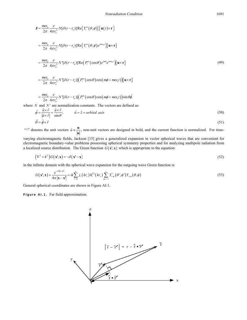
Nonradiation Condition 1691
2
2
2
2
2
[ ( )]Re ,2 4
[ ( )]Re ,2 4
'[ ( )]Re cos2 4
'[ ( )] cos cos2 4
'[ ( )] cos2 4
n
n
mnn
n
im tmnn
n
im tm imnn
n
mnn n
n
mnn
n
m eN r r Y t
r
m eN r r Y e
r
m eN r r P e e
r
m eN r r P m m t
r
m eN r r P
r
J u r
u r
u r
u r
ˆcos sinnm m t
(49)
where N and 'N are normalization constants. The vectors are defined as:
ˆ ˆ ˆ ˆˆ ˆ ˆ; ˆ ˆ sin
u r u ru z orbital axis
u r
(50)
ˆ ˆ r (51)
“^” denotes the unit vectors u u
u, non-unit vectors are designed in bold, and the current function is normalized. For time-
varying electromagnetic fields, Jackson [15] gives a generalized expansion in vector spherical waves that are convenient for electromagnetic boundary-value problems possessing spherical symmetry properties and for analyzing multipole radiation from a localized source distribution. The Green function ,G x' x which is appropriate to the equation:
2 2 ,k G x' x x' x (52)
in the infinite domain with the spherical wave expansion for the outgoing wave Green function is:
1 *, ,
0
, ', ' ,4
ik
m mm
eG ik j kr h kr Y Y
x x'
x' xx x'
(53)
General spherical coordinates are shown in Figure AI.1. Figure AI.1. Far field approximation.
Appendix I 1692
Jackson [15] further gives the general multipole field solution to Maxwell’s equations in a source-free region of empty space with the assumption of a time dependence i te .
, ,,
, ,,
, ,
, ,
E m M mm
E m M mm
ia m f kr a m g kr
k
ia m f kr a m g kr
k
B X X
E X X
(54)
where the cgs units used by Jackson are retained in this section. The radial functions f kr and g kr are of the form:
1 1 2 2g kr A h A h (55)
,mX is the vector spherical harmonic defined by:
, ,
1, ,
1m mY
X L
(56)
where
1
i L r (57)
The coefficients ,Ea m and ,Ma m of Eq. (54) specify the amounts of electric , m multipole and magnetic , m
multipole fields, and are determined by sources and boundary conditions as are the relative proportions in Eq. (55). Jackson gives the result of the electric and magnetic coefficients from the sources as:
2
* 34, ,
1m
E
k ika m Y rj kr j kr ik r j kr d x
r ci
r J
M (58)
and
2
* 34, ,
1
mM
ka m j kr Y d x
c
JL
M (59)
respectively, where the distribution of charge , t x , current , tJ x , and intrinsic magnetization , txM are harmonically
varying sources: te x , te J x , and te xM . From Eq. (49), the charge and intrinsic magnetization terms are zero.
Also, the current , tJ x is in the direction; thus, the ,Ea m coefficient given by Eq. (58) is zero since 0 r J .
Substitution of Eq. (49) into Eq. (59) gives the magnetic multipole coefficient ,Ma m :
22
* 3
ˆ( ) , sin2 44
, ,1
mnn
m nM
m eN r r Y
rka m j kr Y d x
c
L
(60)
wherein the separable time harmonic function of the current is considered separately in Eq. (81). Each mass-density element of the electron moves about the z-axis along a circular orbit of radius sinnr in such a way that , changes at a constant rate. That
is t at time t where nm is the constant angular modulation frequency given in Eq. (49), and
( ) sin cos sin sinn nr t r t r t i j (61)
is the parametric equation of the circular orbit. The relationships between the Cartesian ( ijk ) and spherical ( r e e e ) coordinates
are [16]:
sin cos sin sin cos
cos cos cos sin sin
sin cos
r
e i j k
e i j k
e i j
(62)
The selection rules (Eq. (2.86)) for the conservation of angular momentum must be satisfied during the emission of a single photon of angular momentum :
1 (63)
The photon’s angular momentum given by Eq. (4.1) is:
41Re ( )
8dx
c m r E B* (64)
requiring a matching change in the electron’s angular momentum. With emission, the radius must decrease in order to conserve

Nonradiation Condition 1693
the photon’s energy
E (65)
and the electron’s energy in the inverse-radius Coulomb potential:
2
04
ZeV
r
(66)
The radial electric dipole current for a potentially emitted photon for the selection-rule condition of Eq. (2.86) given by Eq. (2.90) is
cos sinrJ J r
J k e er
(67)
Then, for radiation to occur from the rotating spherical harmonic current (Eq. (49)) while obeying the selection rules and the requirement of an allowed azimuthal-only B (Eq. (2.102)) pertaining to the emission of a single photon, the radiated magnetic field must have e only dependence. Further given Jackson’s Eq. (16.84-16.89) [15] for the relationship of ,Ma m to B , the
components of L in Eq. (60) are restricted to those in the xy-plane, the xL and yL components. It can easily be appreciated that
this result also arises from application of L J to Eq. (67) with the use of the vector identity given by Eq. (16.90) of Jackson [15]: i L J r J (68)
Then, the nonradiation condition tests whether the components of the rotating spherical harmonic current that are parallel to those of Eq. (67) give rise to radiation.
Jackson gives the operator in the xy-plane corresponding to the current motion in this plane and the relations for ,mY [15]:
cotix yL L iL e i
(69)
1, 1 ,m mL Y m m Y (70)
Using Eq. (69), L J of Eq. (59) is
, sin cot , sin
, cot sin sin cot ,
m i m
i m i m
L Y e i Y
e Y i e i Y
(71)
Using Eq. (70) in Eq. (71) gives:
1, sin , cos sin 1 ,m i m mL Y e Y m m Y (72)
The spherical harmonic is given as
,
!2 1, cos cos
4 !m m im m im
m
mY P e N P e
m
(73)
Thus, Eq. (72) is given as:
11, , 1, sin cos cos sin 1 cos i mm i m im mm mL Y e N P e m m N P e
(74)
Substitution of Eq. (74) into Eq. (60) gives:
2
2
,
* 3
11, 1
,21
cos cos
, ( )
sin 1 cos
nM
n
i m imm
mn
i mmm
k ea m N
rc
e N P e
j kr Y r r d x
m m N P e
(75)
Substitution of *, 1 ,mm mY Y and Eq. (73) into Eq. (75) and integration with respect to dr gives:

Appendix I 1694
2
,2
,
0 0 11, 1
,21
cos cos
1 cos sin
sin 1 cos
nM n
i m imm
m m imm
i mmm
eka m Nj kr
c
e N P e
N P e d d
m m N P e
(76)
The integral in Eq. (76) separated in terms of d and d is:
2
, 2
,
0 01, 1
,21
cos cos
1 cos sin
sin 1 cos
nM n
mm
m m im
mm
eka m Nj kr
c
N P
N P d e d
m m N P
(77)
Consider that the d integral is finite and designated by , then Eq. (77) is given as:
22
0
,21
inM n
eka m Nj kr e d
c
(78)
From Eq. (54), the far fields are given by:
,
,
,
,
M m
M m
ia m g kr
ka m g kr
B X
E X
(79)
where ,Ma m is given by Eq. (78).
The power density P t given by the Poynting power vector is:
P t E H (80)
For a pure multipole of order , m , the time-averaged power radiated per solid angle ,dP m
d
given by Eqs. (16.74) and
(16.75) of Jackson [15] is:
22
,2
,,
8 M m
dP m ca m
d k
X
(81)
where ,Ma m is given by Eq. (78).
The modulation function , ,mY is a traveling charge-density wave that moves time harmonically on the surface of
the atomic orbital, spins about the z-axis with frequency n , and modulates at nm corresponding to the term nm t in Eq. (49).
The independent variable is also a term of the argument of the spherical harmonic function as shown in Eq. (49). Consider the entire potentially radiating surface and the single quantized potentially emitted photon that carries all of the conserved angular momentum of and energy given by Planck’s equation. The time dependence of the power is eliminated in Eq. (81), but the boundary condition of the azimuthal spatial integral for ,Ma m over its dependence can also be evaluated in Eqs. (78) and
(81) according to the source current’s space and time dependence using a substitution of variable for . From the azimuthal dependency of the source current corresponding to one period, Eq. (78) that can be written as:
2
0
, cos21
nvT
nM n
eka m Nj kr ks ds
c
(82)
where s is the distance along a current path with the corresponding limit of integration being the angular displacement of the
rotating modulation function during one period nT at the linear velocity in the direction of v , and k is the wavenumber
corresponding to the angular frequency. Thus,

Nonradiation Condition 1695
2
, sin21
nM n n
eka m Nj kr kvT
c
(83)
2
, sin21
nM n
eka m Nj kr ks
c
(84)
In the case that k is the light-like 0k , then /nk c , and the sin ks term in Eq. (84) vanishes for,
nR cT (85)
1nRT c (86)
Rf c (87)
Here n refers to Eq. (48) regarding the angular frequency given by Eq. (1.36) corresponding to the frequency of a potentially
emitted photon as given in Chp. 2. Thus, n n ns vT R r (88)
as given by Eq. (1.279) which is identical to the Haus condition for nonradiation given by Eq. (43), and the photon emission condition given by Eq. (88) is equivalent to that of Eq. (67). Then, the multipole coefficient ,Ma m is zero as it also has to be
according to Eq. (78). For the condition given by Eq. (88), the time-averaged power radiated per solid angle ,dP m
d
given by
Eqs (81) and (84) is zero. There is no radiation.
REFERENCES 1. H. A. Haus, “On the radiation from point charges,” American Journal of Physics, 54, (1986), pp. 1126-1129. 2. R. N. Bracewell, The Fourier Transform and Its Applications, McGraw-Hill Book Company, New York, (1978), pp. 252-
253. 3. W. McC. Siebert, Circuits, Signals, and Systems, The MIT Press, Cambridge, Massachusetts, (1986), p. 415. 4. Y. L. Luke, Integrals of Bessel Functions, McGraw-Hill, New York, (1962), p.22. 5. M. Abramowitz, I. Stegun (3rd Printing 1965), p. 366, Eq. 9.1.10, and p. 255, Eq. 6.1.6. 6. Y. L. Luke, Integrals of Bessel Functions, McGraw-Hill, New York, (1962), p.30. 7. H. Bateman, Tables of Integral Transforms, Vol. III, McGraw-Hill, New York, (1954), p. 33. 8. Personal communication from M. Nansteel February 2011, confirmed by Mathematica by J. Lotoski. 9. G. O. Reynolds, J. B. DeVelis, G. B. Parrent, B. J. Thompson, The New Physical Optics Notebook, SPIE Optical Engineering
Press, (1990). 10. T. A. Abbott, D. J. Griffiths, Am. J. Phys., Vol. 53, No. 12, (1985), pp. 1203-1211. 11. P. Pearle, Foundations of Physics, “Absence of radiationless motions of relativistically rigid classical electron,” Vol. 7, Nos.
11/12, (1977), pp. 931-945. 12. G. Goedecke, Phys. Rev 135B, (1964), p. 281. 13. J. Daboul and J. H. D. Jensen, Z. Physik, Vol. 265, (1973), pp. 455-478. 14. L. C. Shi, J. A. Kong, Applied Electromagnetism, Brooks/Cole Engineering Division, Monterey, CA, (1983), pp. 170-209. 15. J. D. Jackson, Classical Electrodynamics, Second Edition, John Wiley & Sons, New York, (1975), pp. 739-779. 16. G. R. Fowles, Analytical Mechanics, Third Edition, Holt, Rinehart, and Winston, New York, (1977), p. 35.

Appendix I 1696

1697
Appendix II STABILITY AND ABSENCE OF SELF INTERACTION AND SELF ENERGY STABILITY Quantum mechanics does not provide for the stability of matter. The Schrödinger and Dirac solutions violate Maxwell’s equations [1-3] and the textbook argument for stability based on the Heisenberg Uncertainty Principle is false [4-5]. Dirac originally attempted to solve the bound electron physically with stability with respect to radiation according to Maxwell’s equations with the further constraints that it was relativistically invariant and gave rise to electron spin [74]. He and many founders of QM such as Sommerfeld, Bohm, and Weinstein wrongly pursued a planetary model, were unsuccessful, and resorted to the current mathematical-probability-wave model that has many problems [2, 5-18] such as violation of causality and locality, negative kinetic energy states, violation of conservation of energy as shown by the Klein Paradox with an infinite self energy in the electric and magnetic fields as well as instability to radiation.
In contrast, the atomic orbital is stable to radiation as given in Appendix I, and the current pattern is a uniform, minimum-energy equipotential surface, 0
0 ,Y , that gives rise to electron spin. The uniformity proof of the current density
and the corresponding angular momentum that gives rise to electron spin is derived in the Atomic Orbital Equation of Motion For = 0 Based on the Current Vector Field (CVF) section. The atomic orbital geometry and its intrinsic angular momentum of are relativistically invariant as given in the Classical Physics of the de Broglie Relation section and Special Relativistic Correction to the Ionization Energies section, respectively. Furthermore, the centrifugal and Coulombic force-densities that are in balance according to Eq. (1.253) are enormous. From Eqs. (1.35), (1.253), and (1.259), the equivalent pressure HP is:
2 2
12 22 3 5
1 1
12.33 10
4 4He e H
P X N mr m r m a
(1)
This is equivalent to twenty million atmospheres. But, even given the incredible forces of the bound atomic orbital, the energy state can be altered by atomic events such as a resonant collision or the absorption of a resonant photon to form an excited state; whereas, non-resonant collisions and photons cannot change the energy state. Only resonant photons are emitted or absorbed according to the Maxwellian-based conservation rules given in the Excited States section and the Equation of the Photon section to result in an energy state change. No states exist between the resonant states. Moreover, state stability to minor perturbations is an inherent electron property.
Specifically, the electron can only exist as a particle that has mass me with a total magnitude of intrinsic angular momentum of based on the physical laws and constants of the universe (Eqs. (36.1-36.4)). Only specific masses that obey the physical laws of Maxwell’s equations and those of spacetime while satisfying the conservation conditions can exist. The possible particles can be inter-converted, but not broken into smaller particles that do not satisfy these conditions. (See Introduction, Table I.1, and Chapters 32-38.) Chapter 36 (Leptons) provides the conditions for the creation of an electron from a photon that alters spacetime corresponding to a gravitational field contribution. Leptons such as the electron are indivisible, perfectly conducting, and possess an inalienable of intrinsic angular momentum such that any inelastic perturbation involves the entire particle wherein the intrinsic angular momentum remains unchanged. Bound state transitions are allowed involving the exchange of photons between states, each having of angular momentum in their fields. Thus, changes in electron state involve photons that carry the quantized conserved energy and of angular momentum in their fields. A physical approach to solving the structure of the bound electron was followed in Chapter 1 and Appendix I based on the principles of radiation and the corresponding electron state change. These properties maintain the stability of a bound electron to perturbations that do not cause a transition between states and provide that the integral of the physical properties such as the angular momentum of and

Appendix II 1698
energies in the inverse r-squared electric field originating at the nucleus over the entire electron match the boundary conditions. Consequently, the electron atomic orbital behaves as if it has rigidity based on the integrated conserved angular momentum of as well as kinetic energy T wherein T is one-half the magnitude of the potential eV as required for an inverse-squared force
wherein eV is the source of T . Based on the same physical principles, molecular orbitals are stable to non-state-changing
perturbations as given in Chapter 11. It was shown in the Electron g Factor section that as a requirement of the conservation of the electron’s intrinsic angular
momentum corresponding to spin, the magnetic momentum of the electron can only be parallel or antiparallel to an applied magnetic field, and it must link flux in units of the magnetic flux quantum that is the origin of the electron g factor. Similarly, in order to maintain the electron’s intrinsic angular momentum with photon induced states that conserve the photon’s orbital angular momentum by inducing a time harmonic orbital distribution in the electron current, the electron orbital angular momentum integrates to zero over each cycle (Eqs. (1.72) and (1.76)). Moreover, the electron’s velocity changes in at least one of magnitude and direction during a transition. Then, further considering photons that change the electron’s orbital angular momentum and those that don’t, all excited state photons carry angular momentum in their electric and magnetic fields only in quantized units of (Equation of the Photon section) with a corresponding energy of due to the inalienable electron intrinsic angular momentum of . The electron atomic orbital cannot change its state in a continuous manner. Rather any change is quantized (Excited States of the One-Electron Atom (Quantization) section). This condition also applies to any state change mediated by a collision as well as those mediated by photons wherein the collision creates the resonant photon of the excited state with angular momentum and energy conserved. Thus, any potential self interaction of the elements of the current density distribution of the bound electron associated with its intrinsic angular momentum (Atomic Orbital Equation of Motion For = 0 Based on the Current Vector Field (CVF) section) requires the emission of a photon having an angular momentum that is a fraction of and a commensurate fractional change in the electron’s intrinsic angular momentum. This possibility is not allowed as a condition for the existence of the electron.
Furthermore, any allowed self interaction is a radiation-reaction type wherein k is also the lightlike 0k such that /nk c . Any such light-like interaction can only be central. Since the velocity of each point of the electron is the same, the
current of the atomic orbital is confined to a two-dimensional shell in the v c frame as well as the lab frame as given by Eq. (1.280). Since the current is orthogonal to the radial vector at the same radius for each great circle current density element, there is no self interaction. However, as shown in the Electron in Free Space section a radiation-reaction force results when the current is confined to a plane lamina. This force and the conservation of the angular momentum of the free electron and the photon in quantized units of gives rise to the de Broglie relationship as shown in the Classical Physics of the de Broglie Relationship section.
There is no electrostatic self-energy as shown infra, and there is also no magnetic self-energy for the bound electron according to Maxwell’s equations. The magnetic moment is invariant for all states as given in the Special Relativistic Correction to the Ionization Energies section, and the surface current is the source of the discontinuous field that does not exist inside of the electron as given by Eq. (1.136).
( )a bX n H H K (2)
No energy term is associated with the magnetic field unless another source of magnetic field is present. SELF INTERACTION In addition to the electrodynamic interaction between the electron and the nucleus, the self interaction of the electron must be considered in the derivation of Eq. (1.253). The bubble-like geometry of the atomic orbital requires the presence of the proton; otherwise, the electron would exist in the free-electron geometry. As given in the Free Electron section, a free electron comprises a two-dimensional planar lamina with field lines that are discontinuous and orthogonal from opposite surfaces of the lamina such that the Maxwellian condition
1 20
n E E (3)
is satisfied where n is the radial normal unit vector, 1E and 2E are the electric field vectors that are discontinuous at the
opposite surfaces, and is the charge density of the electron corresponding to a total charge of e . There is no self interaction for the free electron that behaves as a two-dimensional perfect conductor. Consider the transformation of the electron’s field lines during binding due to the central field of the proton. The spherical symmetry requires that the field lines of the proton and the bound electron are radial. In order to minimize the energy, the continuous charge density function is a two-dimensional equipotential energy surface with an electric field that is strictly normal-radial (Eq. (2.11)) for 1r r according to Gauss’ law and
Faraday’s law given in the Gauss’ Law in Two Dimensions Equates a Discontinuous Field Due to a Discontinuous Charge Layer Source section. The relationship between the electric field equation and the electron source charge-density function is also given by Eq. (3), Maxwell’s equation in two dimensions [19-21]. As shown in Figure 1.32, 1E , the electric field inside of the atomic
orbital, is zero, 2E , the electric field outside of the atomic orbital, is equivalent to that of a point charge at the origin, and is
the surface charge density corresponding to a total charge of e .

Stability and Absence of Self Interaction and Self Energy 1699
Eq. (3) applies to a perfect conductor. The electron is a perfect conductor, and zero field inside of a perfect conductor is confirmed experimentally. This relation shows that only a 2-D geometry meets the criterion for a fundamental particle and is required for particle production in order to satisfy Maxwell’s equations, special and general relativity, and other first principles such as conservation of energy and momentum as shown in the Gravity, Leptons, and Quarks sections. 2-D is the non-singularity geometry, which is no longer divisible. It is the dimension from which it is not possible to lower the dimensionality without encountering intrinsic field infinities. In this case, there is no electrostatic self interaction since the corresponding potential is discontinuous radially across the surface according to Faraday’s law in the electrostatic limit, and the field is discontinuous, normal, and radial to the charge according to Gauss’ law [19-21]. Thus, only the continuous current density function need be considered. GAUSS’ LAW IN TWO DIMENSIONS EQUATES A DISCONTINUOUS FIELD DUE TO A DISCONTINUOUS CHARGE LAYER SOURCE Haus [19], Jackson [20], and Stratton [21], give the derivation for Gauss’ law in two dimensions. In the electrostatic limit, the pertinent laws are Faraday’s law without magnetic induction and Gauss’ law. The corresponding continuity conditions are:
0 a bn E E (4)
0 0a b
s n E E (5)
where n is the normal unit vector, aE and bE are the electric field vectors that are discontinuous at the opposite surfaces, and
s is the discontinuous two-dimensional surface charge density. The contour enclosing the integration surface over which
Faraday’s law is integrated to obtain Eq. (4) and the integration volume used to obtain Eq. (5) from Gauss’ law are shown in Figures AII.1 and 2, respectively. Figure AII.1. The differential contour intersecting the surface charge density enclosing the integration surface over which Faraday’s law is integrated to obtain Eq. (4) (positive charge is shown by convention).
Figure AII.2. The differential integration volume enclosing the surface charge density having normal n used to obtain Eq. (5) from Gauss’ law.
The conditions that the tangential components of the electric field on either side of the interface are the same according to Eq. (4) requires that the potential is continuous over a surface of discontinuity even if that surface carries a surface charge density. Specifically, as shown for the integration of E around the contour in Figure AII.1, the contributions from A B cancel those from ' 'B A . Thus, the line integral of E from 'A A must be the same as that from 'B B .
'' '
constantA B
A AA B
d d E s E s (6)
If the potential difference across the surface of discontinuity is constant, then the tangential component of E is continuous. Furthermore, since the thickness of the layer 0h , any finite constant potential requires that E is infinite. To avoid this infinity, the continuity condition on is required to be 0a b (7) From Haus [19]:
“Continuity of tangential E is equivalent to continuity of .” To determine the Gauss’ law jump condition through the surface of discontinuity, Gauss’ law is integrated over the

Appendix II 1700
volume shown intersecting the surface in Figure AII.2. The resulting continuity condition (Eq. (5)) is given in terms of the potential using the electrostatic limit where:
E (8)
Eqs. (3) and (5) become
0
a b s
n (9)
From Haus [91]: “At a surface of discontinuity that carries a surface charge density, the normal derivative of the potential is discontinuous.”
SELF FORCE DUE TO A LAYER OF CHARGE WITH NONZERO THICKNESS It is shown by Purcell [22] that a self force does arise in the case of a charge layer that has thickness which is an inescapable problem for the quantum mechanical electron; whereas, the two-dimensional electron atomic orbital has no self interaction. Following the example given by Purcell, consider a spherical surface such as that of a balloon of radius 10 cm charged with about 104 10X additional electrons. Each additional electron is stuck to a rubber molecule that fixes it to the balloon surface where the separation between electrons is about 410 cm . The electric field inside of the sphere is zero according to Gauss’ law since there is no charge here. Outside of the sphere, the electric field given by Gauss’ law is:
2
2 2 20 0
4 57.6
4 4
Q R V m
r r r
r rE i i (10)
where the total charge on the sphere of radius 0.01 R m and the charge density 6 25.10 10 /X C m is 96.41 10 Q X C .
In the case of a two dimensional layer of charge, there is no self force since there is no self charge for this field to act on. But, in the case that the charges of the layer are distributed such that there is a radial distribution, there exists a corresponding radial self force. A fundamental particle is two dimensional, but the layer of the charged balloon and other such charged surfaces cannot be two dimensional and must have finite thickness.
Regarding aggregates of charges on macroscopic objects Purcell [22] states that “real charge layers do not have zero thickness.” He obviously missed the implications for electrons as fundamental particles, even though the absence of self interaction at each radial position was involved in his derivation. And, he states that the self energy corresponding to self force is eliminated “when we replace the actual distribution of discrete elementary charges (the electrons on the rubber balloon) by a perfectly continuous charge distribution [23].”
Purcell uses Gauss’ law in two dimensions as well as Newton’s third law to conclude that there cannot be any charge-charge interaction for charges at the same radial position. According to Purcell, the force within of any two-dimensional spherical shell must be zero. “Coulomb repulsion between charges in the patch is just another example of Newton’s law; the patch as a whole cannot push on itself.” Purcell gives the force on each nth shell as n nd dq dA F E E (11)
where the electric field E is external to the shell—not from the shell itself. Purcell affirms that the correct form of Gauss’ law for the two-dimensional spherical shell is:
1 20
n E E (12)
and that the proper form in the case of the charge layer of finite thickness is:
0
E
(13)
The radial distribution of charge is the source of external field to act on each shell of increasing radius wherein the original charge layer given in Eq. (3) is now considered to have thickness and is modeled as series of radial subshells corresponding to a radial charge density distribution shown in Figure AII.3.

Stability and Absence of Self Interaction and Self Energy 1701
Figure AII.3. Charge pushes against charge in the radial direction such that within the charge layer of density x ,
E x dx E x dx .
Consider that the field is continuously increasing from 1 0 rE i to that at the radius of the largest shell now redefined as R:
2
2 2 20 0 0
4
4 4
Q R
R R
r rE i i (14)
The total force per unit area 'F on the three-dimensional layer of radial thickness 0x is:
0
0
'x
dx F E (15)
Using Eq. (13) gives dE, the change in E through each increment in the radial direction, dx, as dx . Thus, dx in Eq. (15) may be replaced with dE to give:
2
22 2 2
0 0 0 00
1 1 10 0
2 2 2 4 4
EQ Q
dE ER R
F E (16)
where Eq. (10) was used. The self force per unit area of a three-dimensional layer of charge is then proportional to the average of the field inside and outside of the layer of charge which is zero and given by Eq. (10), respectively. Here, the charge density given by Purcell is:
0
0
x
dx (17)
This usage is misleading and should not be confused with a two-dimensional charge density according to Eq. (3). In the case of the charged balloon, the force per unit area is:
2
7 2
0
1' 1.66 10 /
2X N m
F (18)
An expression similar to that given Eq. (16) arises when using Coulomb’s law to calculate the field of a spherical layer of charge at the radius of the shell. The calculation of the field inside of the shell alone implies that the layer must have thickness
so that the field of 1
2Q and self interaction applies. This situation does not arise if Coulomb’s law is applied correctly for
regions outside of a two-dimensional charge discontinuity as given in the Conditions for the Absence or Presence of a Self Force Using Coulomb’s Law section.
Quantum mechanics is internally inconsistent. Electron shielding or self interaction of the electron cloud is ignored in cases involving one electron such as H and 2H , but electron-electron repulsion terms as well as shielding are considered in
multielectron problems such as He and 2H ; even though, the charge densities occupy the same space whether there is one or
more electrons—the only difference being the magnitude. The electron cloud model is also mandatory to achieve neutral scattering despite the internal inconsistency with scattering experiments that the momentum transfer is with the entire mass of the electron as pointed out by Max Born. The subsequent probability-wave model violates special relativity and causality by requiring a point electron to be over all space at once, weighted according to a “guiding” probability density function.
The electron spread over all space must interact with itself since Gauss’ law applied to the volumetric charge density

Appendix II 1702
gives rise to a radial electric field from zero to infinity. Consequently, there is the inescapable problem that the electron cloud is unstable, not to mention the nonphysical nature of the infinities in the electric and magnetic fields of the point electron manifested as a probability cloud distribution. CONDITIONS FOR THE ABSENCE OR PRESENCE OF A SELF FORCE USING COULOMB’S LAW Following the derivation by Fowles [24] for the inverse r-squared gravitational force on a point test mass due to a shell of mass, the electric force of a spherical shell of charge on a test charge q is derived using Coulomb’s law, which is also an inverse r-squared force. The charge-density is integrated over the spherical surface rather than the mass, but the results are of the same form. The Coulomb derivation is also given by Nansteel [25]. Figure AII.4. Coordinates for calculating the field of a spherical shell of charge e of zero thickness.
The shell of zero thickness, total charge e , and radius a shown in Figure AII.4 has a uniform, two-dimensional charge density of:
24
e
a
(19)
centered on the origin O. Based on symmetry, the r-axis is defined as the z-axis, and the azimuthal directions are defined as the xy-plane.
The incremental force dF on the test charge at point P on the z-axis at a distance r from the center O of the spherical shell due to the incremental charge dA at a point Q of the shell is given by:
30
1
4
q dAd
u
F u (20)
where the test charge may lie inside ( r a ) or outside ( r a ) of the 2-D sphere and the force at r a is given by r a since
Coulombs and Gauss’ laws are only defined outside of the charge that is the source of the field, the angle POQ between the z-
axis and point Q is defined as , u is the vector PO
, u u , and the area increment dA on the surface at Q is given by:
2 sindA a d d (21)
where is the azimuthal angle about the z-axis. The vector projections of u from the triangle POQ are:
cos sinr a a z xyu i i (22)
where zi is the unit vector along the z-axis and xyi is the unit vector lying in the plane of POQ and perpendicular to the z-axis.
With the substitution of Eq. (22) into Eq. (20) the incremental force on the test charge is:
2
30
sincos sin
4
q ad r a a d d
u
z xyF i i (23)
and the total force is
2
3
2
0 0 0
sincos sin
4Spherical Shell
q ad r a a d d
u
z xyF F i i (24)
Due to symmetry the azimuthal forces cancel out over each circular integral:
2
0
0d
xyi (25)
Thus, the force is only a function of :

Stability and Absence of Self Interaction and Self Energy 1703
2
30 0
sin cos
2
r aq ad
u
zF i (26)
The integration variable may be changed to u by obtaining the scalar by squaring Eq. (22):
2 22 cos sinu r a a (27)
and then differentiating with respect to :
2 2 cos sin 2 sin cosudu r a a d a a d (28)
Then,
2 2sin cos sin cos sin sinudu ra a d a d ra d (29)
From triangle POQ, the law of cosines gives: 2 2 22 cosu r ur a (30) where cos cosr a u (31) Substitution of Eq. (31) into Eq. (30) gives:
2 2 22 cosu r r r a a (32)
2 2 2
cos2
u r ar a
r
(33)
Multiplication of the right-hand side of Eq. (33) by 1u
u gives:
2 2 2
cos2
r u ar a u
ru
(34)
Substitution of Eqs. (29) and (34) into Eq. (26) gives
2
20
q aI r
r
zF i (35)
where
2
1
4
r a
u r a
r a r aI r du
a u
(36)
Evaluation of Eq. (36) for I r gives
1 1
4 4
1 1 2 2 2 1
4 4
u r a
u r a
r a r a r a r a r a r aI r u r a r a
a u a r a r a
r a r a a a aa a
(37)
Thus, the force on the test charge given by Coulomb’s law is:
2
0
1,
40,
r arqe
r a
zF i (38)
which is the field of a point charge at the origin for radial distances greater than or equal to the radius. This result is consistent with Gauss’ and Faraday’s laws at a two-dimensional layer of charge given by Eq. (3). Then, I r increases by unity as the test
charge is moved from the inside of the sphere ( r a ) to outside ( r a ). But, the behavior of I r :
1,
0,
r a
I r
r a
(39)

Appendix II 1704
suggests the definition
0 0
1 1lim lim
2 2r a r aI a I r I r
(40)
for the case that the test charge lies at the spherical shell. The corresponding force is:
2
2
0
1,
1,
24
0,
r ar
qe r aa
r a
zF i (41)
in conflict with the result of Eq. (3). Although, mathematically Eq. (24) leads to the result of Eq. (41), it is nonphysical, applicable to a charged insulator. To achieve a minimum energy for the bound electron, a perfect conductor, the electric field lines are radial from the surface. The Eq. (38) result is obtained trivially by application of Gauss’ law. A perfectly conducting cavity acts as a Faraday cage wherein experimentally the field inside is zero since the interior contains no charge. The following Gauss-law result holds,
0S V
dA dV
E (42)
2
0
00
4 nr rE i (43)
For a two-dimensional spherical shell that is a perfect conductor the field inside of the spherical cavity, or any hollow conductor for that matter, is zero as shown by Bueche [26]. Thus, the integral given by Eq. (24) is trivially zero since there is no remote action1 of any surface point on another2. Using Eq. (3), the field is given by Eq. (38).
In contrast to the bound-electron case, an ensemble of point charges that are on the surface of a spherical shell insulator gives rise to the result of Eq. (41) with an inherent self interaction due to the remote action of each other surface point charge on any given point charge. An additional self interaction arises when the spherical layer of point charges possesses thickness. A charge density of nonzero thickness is of the form considered by Purcell with:
0
0
2
2
xa
xa
dx
(44)
Specifically, for a linear radial distribution, Gauss’ law gives the force as:
0
0
0 , 2
a
xSpherical Shell r a a
ex
E dA dx
(45)
2
0
24
e
E a
(46)
Thus,
2
0
1
2 4
eE
a (47)
And, the corresponding force on the test charge q at r a is:
2
0
1
2 4
qeF qE
a (48)
This result is also equivalent to the self force given by Purcell in Eq. (16). It is also important to notice that the electric field in both cases is a continuous function of the radial displacement dx such that the final force with the test charge outside of the charge layer is equivalent to that given by Eq. (38) with the exception that the radius includes the thickness of the layer. The caution of confusing the use of as defined in Eqs. (12) and (19) with that given in Eqs. (17) and (44) was also discussed in the Self Force Due to a Layer of Charge with Nonzero Thickness section. 1 Remote action refers to that of a point with a different , from a selected point. 2 The same result arises with the consideration of the cancellation of the bound electron’s field by that of the proton.

Stability and Absence of Self Interaction and Self Energy 1705
In the case that the test charge is a proton at the origin and the charge layer is the electron cloud of the hydrogen atom according to quantum mechanics, the factor of 1/2 must also be considered with the requirement that field lines of the proton end on the electron charge. The proton’s field is continuous and must end in a continuous manner throughout the electron cloud, which results in an infinite-body problem to solve for the form of the cloud and the corresponding energy. Another fatal flaw in quantum mechanics is the corresponding self energy. This problem does not arise in the case of the electron atomic orbital as shown in the Self Energy section. SELF ENERGY The force balance equation can also be arrived at by the familiar minimization of the energy, which demonstrates the absence of a self-energy term for the atomic orbital and the presence of an infinite term for the quantum mechanical solutions. The atomic orbital electron kinetic energy 1T obtained by integration over the mass density at spherical position 'r r (Eq. (1.27)) is:
2
2 2 21 2 2
2
0 0 0
1 1 1' sin
2 4 ' 2 2e
ee
mT v r r r drd d m v
r m r
(49)
where the velocity is given by Eq. (1.35). The electron atomic orbital is a two-dimensional equipotential energy surface at spherical position 'r r . The potential energy is given by integrating Poisson’s equation over the continuous two-dimensional surface charge density given by Eq. (1.27) at the equipotential due to the proton at spherical position 'r r where the electric field of the electron is strictly normal-radial (Eq. (2.11)) for 1r r according to Gauss’ law, and the potential is continuous
across the surface according to Faraday’s law in the electrostatic limit.
2
22
0 0
2
0 0 0
' sin4 4 ' 4
Ze e ZeV r r r drd d
r r r
(50)
And, the energy due to the electrodynamic interaction of the electron and the proton 2T due to their relative motion given by Eq.
(1.35) is
2
22 2
1 1
2 2T mv
mr
(51)
The total energy E is the sum of Eqs. (49-51).
2 2 2
1 2 2 20
1 1
2 4 2e
ZeE T V T
m r r mr
(52)
Then, the minimum energy is obtained by taking the derivative of Eq. (52) and setting it to zero, which is
2 2 2
3 2 304e
Ze
m r r mr
(53)
Eq. (53) can be written in terms of the densities:
2 2
12 2 2 2 3
1 1 1 0 1 1 1
1
4 4 4 4em v e Ze
r r r r r mr
(54)
where 1Z and pm m for the hydrogen atom. Then, Eq. (54) is the same as Eq. (1.253).
As shown in Figure 1.32, the electric field of the proton alone is over all space, and the electric field of the bound electron alone is finite only for 1r r . The radius goes to infinity in the case of the ionized or free electron, and the
corresponding charge and current density functions are given in the Free Electron Section. During binding of the free electron which is a two-dimensional disc lamina, the electron charge distribution becomes that of a 2-D uniform spherical shell of charge, and the electric field of the electron superimposes and cancels part of that of the proton for 1r r as shown in Figure 1.32. The
energy in the electric fields of each of the proton and the electron alone is given as
20
0
1
2eleE dv
E (55)
where E is the electric field of each independently. The binding energy of the hydrogen atom, which is released as photons is given as the change in the electric field energy due to the change in the electric field due to the superposition of the fields of the electron and proton.

Appendix II 1706
1
1
2 2
2 20 0 02 2
0 00
2 2
20 0 1
21 1 1( ) sin
2 2 4 2 4
8 8
r r
ele
r
e eT E dv dv r drd d
r r
e edr
r r
E
(56)
For 1 Hr a as given by Eq. (1.260),
2
0
13.5984 8 H
elee
T E eVa
(57)
In the case of nuclear charge Z , eleE increases by a factor of Z , and the radius given by Eq. (1.260) is 1Ha
rZ
. These
substitutions in Eq. (57) give Eq. (1.264). Eq. (57), matches the experimental binding energy. In contrast, the corresponding energy does not match in the case of
the solutions of the Schrödinger equation. Even if it is assumed that the electron is everywhere at once in order to achieve electroneutrality, which is impossible, the energy stored in the electric field of the electron does not match the binding energy since the average radius of the hydrogen atom in this case is 3/2 the Bohr radius. Even more problematic is that the self-energy in the quantum mechanical electron is infinite wherein the radius in Eq. (56) goes to zero as given by Purcell [27].
REFERENCES 1. V. F. Weisskopf, Reviews of Modern Physics, Vol. 21, No. 2, (1949), pp. 305-315. 2. P. Pearle, Foundations of Physics, “Absence of radiationless motions of relativistically rigid classical electron,” Vol. 7, Nos.
11/12, (1977), pp. 931-945. 3. R. L. Mills, “The fallacy of Feynman’s argument on the stability of the hydrogen atom according to quantum mechanics,”
Annales de la Fondation Louis de Broglie, Vol. 30, No. 2, (2005), pp.129-151; posted at http://www.blacklightpower.com/techpapers.shtml.
4. E. H. Lieb, “The stability of matter,” Reviews of Modern Physics, Vol. 48, No. 4, (1976), pp, 553-569. 5. R. L. Mills, “The fallacy of Feynman’s argument on the stability of the hydrogen atom according to quantum mechanics,”
Annales de la Fondation Louis de Broglie, Vol. 30, No. 2, (2005), pp. 129-151; posted at http://www.blacklightpower.com/techpapers.shtml.
6. F. Laloë, “Do we really understand quantum mechanics? Strange correlations, paradoxes, and theorems,” Am. J. Phys. 69 (6), June 2001, 655-701.
7. R. L. Mills, “Classical quantum mechanics,” Physics Essays, Vol. 16, No. 4, December, (2003), pp. 433-498; posted at http://www.blacklightpower.com/techpapers.shtml.
8. R. L. Mills, “Exact classical quantum mechanical solutions for one- through twenty-electron atoms,” Phys. Essays, Vol. 18, No.3 (2005), 321-361.
9. R. L. Mills, “The Nature of the chemical bond revisited and an alternative Maxwellian approach,” Physics Essays, Vol. 17, (2004), pp. 342-389; posted at http://www.blacklightpower.com/techpapers.shtml.
10. R. L. Mills, “Exact classical quantum mechanical solution for atomic helium which predicts conjugate parameters from a unique solution for the first time,” Phys. Essays, Vol. 21, No. 2, (2008), pp. 103-141.
11. R. L. Mills, The Grand Unified Theory of Classical Quantum Mechanics, May 2005 Edition posted at http://www.blacklightpower.com/theory/bookdownload.shtml.
12. R. L. Mills, “The Grand Unified Theory of Classical Quantum Mechanics,” Int. J. Hydrogen Energy, Vol. 27, No. 5, (2002), pp. 565-590.
13. R. L. Mills, “The nature of free electrons in superfluid helium--a test of quantum mechanics and a basis to review its foundations and make a comparison to classical theory,” Int. J. Hydrogen Energy, Vol. 26, No. 10, (2001), pp. 1059-1096.
14. R. L. Mills, “The hydrogen atom revisited,” Int. J. of Hydrogen Energy, Vol. 25, Issue 12, December, (2000), pp. 1171-1183. 15. R. L. Mills, “Maxwell’s equations and QED: Which is fact and which is fiction,” Physics Essays, Vol. 19, No. 2, (2006),
225-262S. 16. V. F. Weisskopf, Reviews of Modern Physics, Vol. 21, No. 2, (1949), pp. 305-315. 17. A. Einstein, B. Podolsky, N. Rosen, Phys. Rev., Vol. 47, (1935), p. 777. 18. H. Wergeland, “The Klein Paradox Revisited,” Old and New Questions in Physics, Cosmology, Philosophy, and Theoretical
Biology, A. van der Merwe, Editor, Plenum Press, New York, (1983), pp. 503-515. 19. H. A. Haus, J. R. Melcher, “Electromagnetic Fields and Energy,” Department of Electrical Engineering and Computer
Science, Massachusetts Institute of Technology, (1985), Sec. 5.3. 20. J. D. Jackson, Classical Electrodynamics, Second Edition, John Wiley & Sons, New York, (1975), pp. 17-22. 21. J. A. Stratton, Electromagnetic Theory, McGraw-Hill Book Company, (1941), p. 195. 22. E. Purcell, Electricity and Magnetism, McGraw-Hill, New York, (1985), pp. 29-31. 23. E. Purcell, Electricity and Magnetism, McGraw-Hill, New York, (1985), p. 33. 24. G. R. Fowles, Analytical Mechanics, Third Edition, Holt, Rinehart, and Winston, New York, (1977), pp. 138-140.

Stability and Absence of Self Interaction and Self Energy 1707
25. M. Nansteel, available at http://www.blacklightpower.com/pdf/Electrical_Field_Due_to_Spherical_Surface_Charge.pdf. 26. F. J. Bueche, Introduction to Physics for Scientists and Engineers, McGraw-Hill, New York, (1975), pp. 351-356. 27. E. Purcell, Electricity and Magnetism, McGraw-Hill, New York, (1985), pp. 31-33.

Appendix II 1708
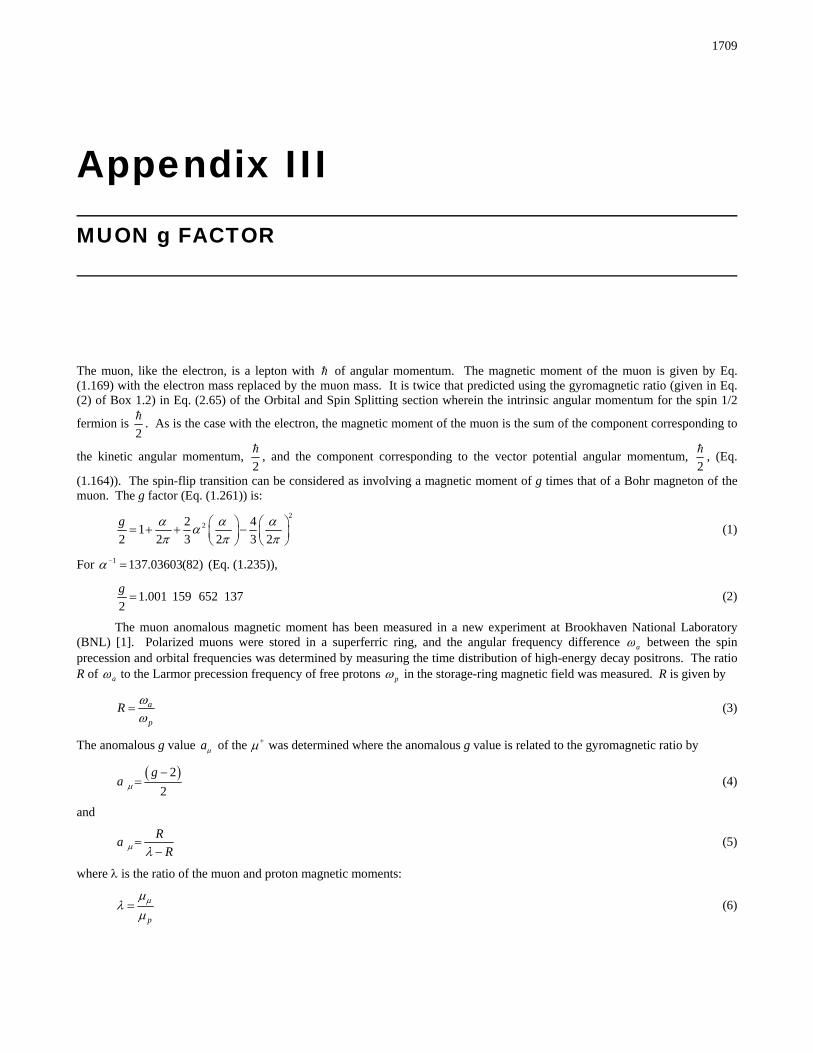
1709
Appendix III MUON g FACTOR The muon, like the electron, is a lepton with of angular momentum. The magnetic moment of the muon is given by Eq. (1.169) with the electron mass replaced by the muon mass. It is twice that predicted using the gyromagnetic ratio (given in Eq. (2) of Box 1.2) in Eq. (2.65) of the Orbital and Spin Splitting section wherein the intrinsic angular momentum for the spin 1/2
fermion is 2
. As is the case with the electron, the magnetic moment of the muon is the sum of the component corresponding to
the kinetic angular momentum, 2
, and the component corresponding to the vector potential angular momentum,
2
, (Eq.
(1.164)). The spin-flip transition can be considered as involving a magnetic moment of g times that of a Bohr magneton of the muon. The g factor (Eq. (1.261)) is:
2
22 41
2 2 3 2 3 2
g
(1)
For 1 137.03603(82) (Eq. (1.235)),
1.001 159 652 1372
g (2)
The muon anomalous magnetic moment has been measured in a new experiment at Brookhaven National Laboratory (BNL) [1]. Polarized muons were stored in a superferric ring, and the angular frequency difference a between the spin precession and orbital frequencies was determined by measuring the time distribution of high-energy decay positrons. The ratio R of a to the Larmor precession frequency of free protons p in the storage-ring magnetic field was measured. R is given by
a
p
R
(3)
The anomalous g value a of the was determined where the anomalous g value is related to the gyromagnetic ratio by
2
2
ga
(4)
and
R
aR
(5)
where is the ratio of the muon and proton magnetic moments:
p
(6)

Appendix III 1710
According to Carey et al. [1], “For polarized muons moving in a uniform magnetic field B
, which is perpendicular to the muon spin direction and to the plane of the orbit, and with an electric quadrupole field E
for vertical focusing, the angular frequency
difference, a , between the spin precession frequency s and the cyclotron frequency c is given by:
2
1
1ae
a am
B B E
(7)
The dependence of a on the electric field is eliminated by storing muons with the ‘magic’ 29.3, which corresponds to a muon momentum p 3.09 GeV /c . Hence measurement of a and of B determines a .”
Based on Lorentz covariance Jackson [2] gives the BMT equation which is the relativistic equation of motion for spin in uniform or slowly varying external fields. The rate of change of the component of spin s parallel to the velocity may be
determined from the BMT equation. This is the longitudinal polarization or net helicity of the particle. If is a unit vector in
the direction of v
c, the longitudinal polarization is s . It changes in time because s changes and also changes. The
BMT equation in cgs units gives:
1ˆ ˆ12 2
d e g g
dt mc
s s B E (8)
where s is the component of s perpendicular to the velocity. Eq. (8) demonstrates a remarkable property of a particle with g 2. In a purely magnetic field, the spin precesses in such a manner that the longitudinal polarization remains constant, whatever the motion of the particle. If the particle is relativistic ( 1), even the presence of an electric field causes the longitudinal polarization to change only very slowly, at a rate proportional to 2 times the electric field component perpendicular to v.
The “magic” given by Eq. (8) wherein the contribution to the change of the longitudinal polarization by the electric quadrupole focusing fields are eliminated occurs when:
1
02
g
(9)
where g is the muon g factor which is required to be different from the electron g factor in the standard model due to the
dependence of the mass dependent interaction of each lepton with vacuum polarizations due to virtual particles. For example, the muon is much heavier than the electron, and so high energy (short distance) effects due to strong and weak interactions are more important here [3]. Also, according to the BNL collaboration [1]:
“The hadronic contribution and uncertainty are dominated by the single vacuum polarization loop with hadrons present, which is determined from a dispersion relationship using data from annihilation to hadrons and from hadronic decay. A contribution from higher order hadronic vacuum polarization and light-by-light scattering must be included”
The BNL Muon (g-2) Collaboration [1] used a “magic” 29.3 which satisfied Eq. (9) identically for g2
; however, their
assumption that this condition eliminated the affect of the electrostatic field on a is flawed as shown below. The relativistic factor is given by:
2
1
1
(10)
where
v
c (11)
Substitution of Eq. (9) into Eq. (10) gives:
1
21
g
(12)
and
2
2 11
g
(13)

Muon g Factor 1711
From the BNL99 results and the average of the CERN and BNL97 results [1] an estimated value of 2
g is:
1.001165932
g (14)
Substitution of Eq. (14) into Eq. (12) gives the “magic” as:
29.3033176 (15)
and from Eq. (13),
0.999417544
(16)
As shown in the Electron g Factor section, in the case of an exact balance between the Lorentz force (Eq. (1.183)) and the electric force corresponding to the Hall voltage (Eq. (1.184)), the superconducting condition is met when:
Ev
B
(17)
which in cgs units is:
BvE B
c
(18)
Consider the case that the g factor for the muon and the electron are the same and the “magic” 29.3 selected by the BNL
Muon (g-2) Collaboration which satisfied Eq. (9) identically for 2
g (Eq. (1.229)) does not satisfy Eq. (9) for 2
eg given by the
experimental value (Eq. (27)). In this case, the second term of Eq. (8) contributes to a . With eg g and , the BMT
equation is:
1ˆ ˆ12 2
e eggd e
dt mc
s s B E (19)
Since B is parallel to s and since E and s are anti-parallel, the electric field from Eq. (18) is:
ˆ E B (20)
Figure AIII.1. Coordinate system of crossed electric field, xE , corresponding to the Hall voltage, magnetic flux, zB , due to
the applied field, the velocity, yv , in the direction, and s where BE .
Then
2
ˆ ˆ1 12 2
e eggd e
dt mc
s s B (21)
2
ˆ2 2
eegge
mc
s B (22)
2 ˆ12
ege
mc
s B (23)
In the case that eg g g , the term in E of Eq. (8)

Appendix III 1712
ˆ ˆ12
gd e
dt mc
s s B (24)
vanishes and a change in longitudinal polarization due to the finite electric term can be considered as an additional term to the
electron g factor which gives rise to an effective g factor corresponding to.2
g Comparison of Eq. (23) and Eq. (24) gives the
effective value of 2
g which is the predicted experimental value for 2
g :
21 12 2
eg g
(25)
21 12 2
eg g
(26)
Eq. (19), which gives the predicted experimental value for 2
g (Eq. (26)), corresponds to the experimental situation of the BNL
measurement of 2
g . The experimental value of 2
eg [4] is:
1.001 159 652 188(4)2
eg (27)
Substitution of 2
eg and given by Eq. (27) and Eq. (16), respectively, into Eq. (26) gives the calculated effective muon g
factor which is:
1.001 165 9232
g (28)
The calculated result based on the equivalence of the muon and electron g factors is in agreement with the result of Carey et al. [1]:
1.001 165 925 (15)2
g (29)
Rather than indicating an expanded plethora of postulated super-symmetry virtual particles which make contributions such as smuon-neutralino and sneutrino-chargino loops as suggested by Brown et al. [5], the deviation of the experimental value
of 2
g from that of the standard model prediction simply indicates that the muon g factor is identical to the electron g factor.
This could have been spotted immediately had the objectivity of the experimental design been given precedence over the assumption of the validity of the standard model. Given the ad hoc nonphysical nature of QED (See Refs. [6-7]) and the internal inconsistency of the theoretical basis of this experiment regarding using the classical BMT equation in a test of nonclassical QED, more scrutiny was especially warranted.
From Eqs. (26), (27), and (16), the difference between 2
g and 2eg
due to the finite electric term of Eqs. (8) and (19)
with eg g is:
21 0.00000627052 2 2
e eg g g
(30)
With the equivalence of the muon g factor and the electron g factor, the possibilities are limited for the occurrence of internal
consistency during the determination of 2
g using the BMT equation with the flawed assumption that 2 2
eg g . Consider the
case of Eq. (9) with eg g g and u with the corresponding “magic” given by Eqs. (10-13). An equation equivalent
to Eq. (30) that gives rise to an internally consistent experimental observation of an effective muon g factor corresponding to
u is:
2
1 20.0000062705
22
egg
g
g
(31)

Muon g Factor 1713
21 0.0000062705
2
eg
g (32)
where g is the muon anomalous g factor selected before the experiment to fix the “magic” , 0.0000062705 given by Eq.
(32) (also see Eq. (30)) is the difference between the projected experimental value of 2
g and the experimentally measured value
of 2
eg. The experimental value of
2eg
from Eq. (27) and the selected value of 2
g from Eq. (14) satisfy Eqs. (31-32) and are in
close agreement with the experimental value of 2
g determined by Carey et al. [1] (Eqs. (28-29)). The “magic” of BNL
which gave an internally consistent but misinterpreted result was most likely arrived at by trial and error. Consider the following
relationship between and 2
2
yg of the “magic” that follows from Eq. (32):
21
2
e
y
g
g (33)
where
22
2 2e
gg
(34)
and eg is the experimentally measured electron anomalous g factor and g is the projected experimental value of the muon
anomalous g factor based on g , the selected value the muon anomalous g factor to fix the “magic” . A plot of versus
2
2yg
from Eq. (33) is shown in Figure AIII.2.
Figure AIII.2. Plot of versus 2
2
g of the “magic” from Eq. (33).
Only a narrow range of values of 2
2
g about the value of
2
2
g measured by Carey et al. [1] are internally consistent.
Similar misinterpretations of data based on a bias towards quantum theory are described in the Schrödinger “Black” Cats section. For example, NIST claimed to have placed a 9Be ion in two places at once when in reality an applied magnetic field and a potential well were found which forced a resonance between an oscillatory and a Stern-Gerlach transition. And, the resulting interference pattern in the fluorescence emission was misinterpreted as indicating that the ion was in two widely separated positions simultaneously [8]. The BNL experiment should be repeated to determine the dependence of a on the “magic” . The current BNL results and classical theory support the equivalence of the electron and muon g factors.

Appendix III 1714
EXPERIMENTAL DETERMINATION OF THE PROPER [9] The angular frequency difference between the spin procession frequency and the cyclotron frequency, [4], is:
2
1
1ae
a amc
B B E
(35)
Introducing the velocity ratio, , and g,
2
22
1 , 11 2
ga
(36)
yields
2
11
2 2ae g g
mc
B B E
(37)
The unique value of for which the term in E vanishes is * :
*2
1
2
g
(38)
For *
**2
11a
e
mc
B
(39)
Taking the magnitude results in
**2
11a
eB
mc
(40)
The experimental measurement of the frequency difference for various allows the graphical determination of * , (See Figure AIII.3), with no assumption regarding g. Figure AIII.3. Plot of the experimental measurement of the frequency difference for various which allows the graphical determination of * .
*
a()
B11mce
2
REFERENCES 1. R. M. Carey et al., Muon (g-2) Collaboration, “New measurement of the anomalous magnetic moment of the positive muon,”
Phys. Rev. Lett., Vol. 82, (1999), pp. 1632-1635. 2. J. D. Jackson, Classical Electrodynamics, Second Edition, John Wiley & Sons, New York, (1975), pp. 556-560. 3. G. P. Lepage, Theoretical advances in quantum electrodynamics, International Conference on Atomic Physics, Atomic
Physics Proceedings, Singapore, World Scientific, Vol. 7, (1981), pp. 297-311. 4. R. S. Van Dyck, Jr., P. Schwinberg, H. Dehmelt, “New high precision comparison of electron and positron g factors,” Phys.
Rev. Lett., Vol. 59, (1987), p. 26-29. 5. H. N. Brown et al., Muon (g-2) Collaboration, “Precise measurement of the positive muon anomalous magnetic moment,”
Phys. Rev. D62, 091101, (2000). 6. R. L. Mills, “Maxwell’s Equations and QED: Which is Fact and Which is Fiction,” Physics Essays, Vol. 19, (2006), pp. 225-
262. 7. R. L. Mills, “The Fallacy of Feynman's Argument on the Stability of the Hydrogen Atom According to Quantum
Mechanics,” Annales de la Fondation Louis de Broglie, Vol. 30, No. 2, (2005), pp. 129-151. 8. C. Monroe, D. M. Meekhof, B. E. King, D. J. Wineland, Science, Vol. 272, (1996), pp. 1131-1135. 9. M. Nansteel, BlackLight Power, Inc., Cranbury, NJ, Personal Communication, May, (2001).

1715
Appendix IV ANALYTICAL EQUATIONS TO GENERATE THE FREE ELECTRON CURRENT-VECTOR FIELD AND THE ANGULAR-MOMENTUM-DENSITY FUNCTION 0
0 ,
Y
ROTATION OF A GREAT CIRCLE IN THE XY-PLANE ABOUT THE ,0 ,x y zi i i -AXIS
BY 2 With the electron current in the counter clockwise direction, the Larmor precession of the angular momentum vector of the free
electron is about two axes simultaneously, the ,0 ,x y zi i i -axis and the laboratory-frame z-axis defined by the direction of the
applied magnetic field. The precessions are about the opposite axes with the current in the opposite direction. The motion generates CVFs equivalent to those of the bound electron given in the Atomic Orbital Equation of Motion for = 0 Based on the Current Vector Field (CVF) section. Over one time period, the first motion sweeps out the equivalent of a BECVF, and the rotation about the z-axis sweeps out the equivalent of an OCVF. The combined motions sweep out the equivalent of the convolution of the BECVF with the OCVF, a distribution having the angular momentum equivalent of 0
0 ( , ) Y of the bound
electron. The electron may flip between the two states wherein the BECVF, OCVF, and 00 ( , ) Y precession distributions
developed infra apply to both states, but the currents are opposite. Specifically, the Larmor precession of the free electron with the current in the counter clockwise direction corresponds to
the two superimposed independent time-harmonic rotations of the plane-lamina disc initially in the xy-plane. One is about the
,0 ,x y zi i i -axis by 2 wherein the angular momentum vector of the free electron that is perpendicular to the plane-lamina of its
current sweeps out a cone about the ,0 ,x y zi i i -axis. The plane-lamina is comprised of concentric great circle current loops
each of a radius given by the continuous variable for 00 . For each great circle, the first Larmor precession generates
the equivalent vector-field pattern as that of a BECVF. Simultaneously, the distribution corresponding to the first rotation
precesses or rotates about the laboratory z-axis defined by the applied magnetic field direction wherein the ,0 ,x y zi i i -axis
sweeps out a cone about the z-axis. Over one time period, the rotational motion about the z-axis generates the equivalent vector-field pattern as that of an OCVF of the bound electron. The combined motions over time generate the equivalent distribution and angular momentum as those of 0
0 ( , )Y of the bound electron given by the convolution of the OCVF with the BECVF.
The rotation of a great circle in the xy-plane about the ,0 ,x y zi i -axis by 2 generates a free electron BECVF
corresponding to the precession motion with its resultant angular momentum of 2 along the ,0 ,x y zi i i -axis having
components of xyL and zL . Equally valid is the substitution of the ,0 , x y zi i i -axis for the ,0 ,x y zi i -axis since the
corresponding orthogonal BECVFs have the same distribution and are simply related by a half cycle of precession motion about the z-axis. Both will be considered.

Appendix IV 1716
The BECVF corresponding to the ,0 ,x y zi i i -axis over 2 will be generated first following the procedure given in
Fowles [1] and using the matrices given by Eqs. (1.80-1.82). The rotational matrix about the ,0 ,x y zi i i -axis by ,
,0 ,
Rx y zi i i
, is given by:
,0 , 4 4y z yR R R R
x y zi i i
(1)
Then, using Eqs. (1) and Eqs. (1.81-1.82), the great circle basis elements and rotational matrix are given by: BECVF MATRICES (
,0 , Rx y zi i i
)
1 cos sin 1 cos
2 2 2 22' cos
sin sin' cos sin
2 2
' 01 cos sin 1 cos
2 2 2 22
x
y
z
(2)
Using Eq. (2), the BECVF matrix representation of the convolution is given by:
2
,0 , , ,00 1
lim
m
basisM
m
BECVF R GC mx y z x y zi i i i i i
(3)
wherein ,0 ,
Rx y zi i i
is the rotational matrix about the ,0 ,
Rx y zi i i
-axis, , ,0
basisGCx y zi i i
is the great circle basis element initially in
the xy-plane, and designates the convolution with the delta function of the infinitesimal incremental angle Mm . The
integral form of the convolution is
2
2
,0 , , ,00 10
lim
m
basisM
m
BECVF R GC m dx y z x y zi i i i i i
(4)
The integration gives the infinite sum of great circles that constitute the BECVF:
2
,0 , , ,00 1
lim
m
basisM
m
BECVF R m GCx y z x y zi i i i i i
(5)
The current pattern for the rotation of the xy-plane great circle about the ,0 ,x y zi i i -axis is shown in Figure IV.1 wherein is
varied from 0 to 2 .
Figure IV.1. The current pattern for the rotation of the xy-plane great circle about the ,0 ,x y zi i i -axis (Eqs. (2) and (5))
shown with 6 degree increments of from the perspective of looking along the z-axis. The great circle current loop that served as a basis element that was initially in the xy-plane is shown as red.

Analytical Equations to Generate the Free Electron Current-Vector Field and the Uniform Angular-Momentum-Density Function
1717
CONICAL SURFACES FORMED BY VARIATION OF The rotation of the free-electron disc having a continuous progression of larger current loops along forms two conical
surfaces over a period that join at the origin and face in the opposite directions along the ,0 ,x y zi i i -axis, the axis of rotation, as
shown in Figure IV.2. At each position of 0 , there exists a BECVF of that radius that is concentric to the one of
infinitesimally larger radius to the limit at 0 . The BECVF at each position generated over a period by the Larmor
precession about the ,0 ,x y zi i i - axis by 2 is given by Eqs. (2) and (5). The conical surfaces were generated by varying in
Eqs. (2) and (5). Figure IV.2. The two conical surfaces formed by rotation of the plane-lamina disc comprised of concentric great circles
about the ,0 ,x y zi i i -axis that join at the origin and face in the opposite directions along the axis of rotation, the ,0 ,x y zi i i -
axis.
ROTATION OF A GREAT CIRCLE IN THE XY-PLANE ABOUT THE ,0 , x y zi i i -AXIS
BY 2 Similarly, the Larmor precession of the free electron about the z-axis also corresponds to the time-harmonic rotation of the
plane-lamina disc about the ,0 , x y zi i i -axis by 2 . The Larmor precession of the plane-lamina comprised of concentric
great-circle current loops each of a radius given by the continuous variable for 00 generates the equivalent BECVF.
The rotational matrix about the ,0 , x y zi i i -axis by , ,0 ,
Rx y zi i i
, is given by
,0 , 4 4
y z yR R R Rx y zi i i
(6)
Then, using Eqs. (6) and Eqs. (1.81-1.82), the great circle basis elements and rotational matrix are given by

Appendix IV 1718
BECVF MATRICES (
,0 ,
R
x y zi i i)
1 cos sin 1 cos+ +
2 2 2 22' cos
sin sin' cos sin
2 2
' 01 cos sin 1 cos
+ +2 2 2 22
x
y
z
(7)
Using Eq. (7), the BECVF matrix representation of the convolution is given by:
2
,0 , , ,00 1
lim
m
basisM
m
BECVF R GC mx y z x y zi i i i i i
(8)
wherein ,0 ,
Rx y zi i i
is the rotational matrix about the ,0 ,
Rx y zi i i
-axis, , ,0
basisGCx y zi i i
is the great circle basis element initially in
the xy-plane, and designates the convolution with the delta function of the infinitesimal incremental angle Mm . The
integral form of the convolution is
22
,0 , , ,00 10
lim
m
basisM
m
BECVF R GC m dx y z x y zi i i i i i
(9)
The integration gives the infinite sum of great circles that constitute the BECVF:
2
,0 , , ,00 1
lim
m
basisM
m
BECVF R m GCx y z x y zi i i i i i
(10)
The current pattern for the rotation of the xy-plane great circle about the ,0 , x y zi i i -axis is shown in Figure IV.3 wherein is
varied from 0 to 2 .
Figure IV.3. The current pattern for the rotation of the xy-plane great circle about the ,0 , x y zi i i -axis (Eqs. (7) and (10))
shown with 6 degree increments of from the perspective of looking along the z-axis. The great circle current loop that served as a basis element that was initially in the xy-plane is shown as red.

Analytical Equations to Generate the Free Electron Current-Vector Field and the Uniform Angular-Momentum-Density Function
1719
CONICAL SURFACES FORMED BY VARIATION OF The rotation of the free-electron disc having a continuous progression of larger current loops along forms two conical
surfaces over a period that join at the origin and face in the opposite directions along the ,0 , x y zi i i -axis, the axis of rotation,
as shown in Figure IV.4. At each position of 0 , there exists a BECVF of that radius that is concentric to the one of
infinitesimally larger radius to the limit at 0 . The BECVF at each position generated over a period by the Larmor
precession about the ,0 , x y zi i i - axis by 2 is given by Eqs. (7) and (10). The conical surfaces were generated by varying
in Eqs. (7) and (10). Figure IV.4. The two conical surfaces formed by rotation of the plane-lamina disc comprised of concentric great circles
about the ,0 , x y zi i i -axis that join at the origin and face in the opposite directions along the axis of rotation, the ,0 , x y zi i i -
axis.
THE MOMENTUM-DENSITY FUNCTION 00 ( , ) Y
Each basis-element great circle of the plane lamina current-density function of the free electron at a position generates the BECVF that is perpendicular to the rotation axis used for the generation of the distribution of great circles. The rotation of a
great circle in the xy-plane about the ,0 ,x y zi i -axis by 2 generates a precessing free electron BECVF corresponding to a
Bohr magneton of magnetic moment about the z-axis as given in the Rotation of a Great Circle in the xy-Plane about the
,0 ,x y zi i i -Axis by 2 section. An OCVF is formed by the 2 rotation of a great circle perpendicular to the ,0 ,x y zi i -axis
about the z-axis. Using the same type of convolution of CVFs as in the Atomic Orbital Equation of Motion for = 0 Based on the Current Vector Field (CVF) section, the function 0
0 , Y corresponding to the motion of a free electron is obtained by
convolving the BECVF given by Eqs. (2) and (5) as the basis element with the OCVF. This operation is equivalent to incrementally rotating the BECVF about the z-axis by 2 .
Similarly, the rotation of a great circle in the xy-plane about the ,0 , x y zi i -axis by 2 generates the orthogonal
BECVF given in the Rotation of a Great Circle in the xy-Plane about the ,0 , x y zi i -Axis by 2 section. An OCVF is also
formed by the 2 rotation of a great circle perpendicular to the ,0 , x y zi i -axis about the z-axis. The function 00 , Y
corresponding to the motion of a free electron is obtained by convolving the BECVF given by Eqs. (7) and (10) as the basis element with the OCVF. This operation is equivalent to incrementally rotating the BECVF about the z-axis by 2 .

Appendix IV 1720
MATRICES TO VISUALIZE THE MOMENTUM-DENSITY OF 00 , Y FOR THE
COMBINED PRECESSION MOTION OF THE FREE ELECTRON ABOUT THE ,0 ,x y zi i i -
AXIS AND Z-AXIS The free BECVFs are given by Eqs. (2) and (5) and Eqs. (7) and (10). Consider the case of the 0
0 , Y momentum-density
pattern for the combined precessional motion of the free electron about the ,0 ,x y zi i i -axis and z-axis having the magnetic
moment of B on the z-axis. The free electron OCVF is given by rotating a basis-element great circle that is perpendicular to
the ,0 ,x y zi i i -axis about the z-axis by 2 . The transformation matrix to give the OCVF is generated by the combined rotation
of a great circle in the xy-plane about the y-axis by 4
then about the z-axis by . The coordinates of the great circle basis
element to generate the OCVF are given by the matrix that rotates a great circle in the xy-plane about the y-axis by 4
:
T
T Tcos cos', ', ' , sin , cos , sin ,0
42 2
yx y z R (11)
The OCVF is generated by rotating the basis element great circle given by Eq. (11) about the z-axis using zR over the span
of 2 . Using Eqs. (11) and Eq. (1.82), the great circle basis elements and rotational matrix are given by: OCVF MATRICES ( zR )
coscos sin 0' 2
' sin cos 0 sin
' cos 0 0 1
2
x
y
z
(12)
Using Eq. (12), the infinite sum of great circles representation of the OCVF is given by:
2
1 1, ,0 1 2 2
lim
m
basisz M
m
OCVF R m GCx y zi i i
(13)
The current pattern for the 2 rotation of the great circle perpendicular to the ,0 ,x y zi i i -axis about the z-axis is shown in
Figure IV.5 wherein is varied from 0 to 2 .
Figure IV.5. The current pattern given by Eqs. (12) and (13) shown with 6 degree increments of from the perspective of looking along the z-axis. The great circle current loop that served as a basis element that was initially in the xy-plane before applying Eq. (11) and then Eq. (12) is shown as red.

Analytical Equations to Generate the Free Electron Current-Vector Field and the Uniform Angular-Momentum-Density Function
1721
CONVOLUTION GENERATION OF 00 ( , ) Y
The great-circle distribution 00 ( , ) Y is generated by the convolution of either BECVF with the corresponding OCVF over a
2 span. The convolution operator treats each CVF independently and results in the placement of a BECVF at each great circle of the OCVF such that momentum density pattern over time matches the bound-electron current pattern 0
0 ( , )Y , the initial
angular momentum matches that of the great circle basis element of the OCVF, and the angular momentum rotates about the z-axis along the initial resultant angular momentum axis. This is achieved by rotating the orientation, phase, and vector-matched basis-element, the BECVF, about the same axis as that which generated the OCVF from the corresponding basis element great circle. Thus, the corresponding BECVF replaces the great circle basis element initially perpendicular to one of the orthogonal
axes such as the ,0 ,x y zi i i -axis and matches its resultant angular momentum of 2 along the ,0 ,x y zi i i -axis having
components of xyL and zL . Then, 00 ( , ) Y is generated by rotation of the BECVF about the z-axis by an infinite set of
infinitesimal increments of the rotational angle over the 2 span such that coverage of the spherical surface is complete. The corresponding convolution operator comprises an autocorrelation-type function that demonstrates the resulting azimuthal uniformity of the distribution when the orthonormality of the operator matrices is utilized as shown in the Azimuthal Uniformity Proof of 0
0 ( , ) Y section.
The operator to form 00 ( , ) Y comprises the BECVF convolution [2] of the rotational matrix of the great circles basis
element about the ,0 ,x y zi i i -axis with an infinite series of delta functions of argument of the infinitesimal angular increment
that is further convolved with the OCVF convolution of the rotational matrix of the great circles basis element about the z-axis with an infinite series of delta functions of argument of the infinitesimal angular increment. Using the BECVF matrix representation of its convolution operation (Eqs. (2) and (5)) and the OCVF matrix representation of its convolution operation (Eqs. (12) and (13)), the 0
0 ( , ) Y matrix representation of the convolution is given by:
2
1 1
, ,0 1 2 2
00 2
,0 , , ,0
0 1
lim
( , )
lim
m
basisz M
m
n
basisN
n
R GC m
Y OCVF BECVF
R GC n
x y z
x y z x y z
i i i
i i i i i i
(14)
where the commutative property of convolutions [2] allows for the interchange of the order of CVFs, but the rotational matrices are noncommutative [1]. The integral form of the convolution is:
22
1 1
, , 0 10 2 2
00 2
2
,0 , , ,0
0 10
lim
( , )
lim
m
basis OCVFz M
m
n
basis BECVFN
n
R GC m d
Y
R GC n d
x y z
x y z x y z
i i i
i i i i i i
(15)
2 2
2 20
0 1 2 1 2 1 2,0 , , ,00 01 1 0 0
( , ) lim lim
m n
basis OCVF BECVFz M N
m n
Y d d R R GC m n
x y z x y zi i i i i i (16)
The integration gives the infinite double sum of great circles that constitute 00 ( , ) Y :
2 2
0 0 ,0 , , ,0
0 01 1
( , ) lim lim
m n
OCVF BECVF basisz M N
m n
Y R m R n GCx y z x y zi i i i i i
(17)
The positions of the basis-element great circle over time comprises a continuous distribution. However, using Eq. (17), a discrete representation of the current distribution 0
0 ( , ) Y that shows a finite number of current elements over time can be
generated by showing the BECVF as a finite sum of the convolved great circle elements using Eqs. (2) and (5) and by showing the continuous convolution of the BECVF with the OCVF as a superposition of discrete incremental rotations of the position of the BECVF rotated according to Eqs. (12) and (13) corresponding to the matrix which generated the OCVF. In the case that the discrete representation of the BECVF comprises N great circles and the number of convolved BECVF elements is M , the representation of the azimuthally uniform current density function showing current loops is given by Eq. (18) and shown in Figures IV.6 and IV.7. The corresponding mass(momentum) density is also represented by Figures IV.6 and IV.7 wherein the

Appendix IV 1722
charge and mass are interchangeable by the conversion factor /em e . Computer modeling of the analytical equations to generate
the free electron current vector fields and the azimuthally uniform momentum-density function 00 , Y is available on the web
[3]:
m=M
m=1
2 2 cos sin 0
'
2 2' sin cos 0
'
0 0 1
2cos
1
2 2
m m
M Mx
m my
M M
z
nN
n
2 2 sin cos
1
2 22
2 2 sin sin
2 cos
2 2
2 2 2cos sin cos
1 1
2 2 2 22
n nN N
n nnN NN
n n nN N N
n=N
=1
cos
sin
0
(18)
Figures IV.6 and IV.7. Representations of the current pattern of the 0
0 ( , ) Y free electron motion over a period of both
precessional motions shown with 30 degree increments ( 12 N M in Eq. (18)) of the angle to generate the free electron BECVF corresponding to Eqs. (2) and (5) and 30 degree increments of the rotation of this basis element about the z-axis corresponding to Eqs. (12) and (13). The great circle current loop that served as a basis element that was initially in the xy-plane of each free electron BECVF is shown as red Figure IV.6 The perspective is along the z-axis. Figure IV.7 The perspective is along the x-axis.

Analytical Equations to Generate the Free Electron Current-Vector Field and the Uniform Angular-Momentum-Density Function
1723
MATRICES TO VISUALIZE THE MOMENTUM-DENSITY OF 00 , Y FOR THE
COMBINED PRECESSION MOTION OF THE FREE ELECTRON ABOUT THE ,0 , x y zi i i -AXIS AND Z-AXIS Consider the case of the 0
0 , Y momentum-density pattern for the combined precessional motion of the free electron about the
,0 , x y zi i i -axis and z-axis having the magnetic moment of B on the z-axis. The corresponding free BECVF is given by Eqs.
(7) and (10). The free electron OCVF is given by rotating a basis-element great circle that is perpendicular to the ,0 , x y zi i i -
axis about the z-axis by 2 . The transformation matrix to give the OCVF is generated by the combined rotation of a great circle
in the xy-plane about the y-axis by 4
then about the z-axis by . The coordinates of the great circle basis element to generate
the OCVF are given by the matrix that rotates a great circle in the xy-plane about the y-axis by 4
:
T
T Tcos cos', ', ' , sin , cos , sin ,0
42 2
yx y z R (19)
The OCVF is generated by rotating the basis element great circle given by Eq. (19) about the z-axis using zR over the span
of 2 . Using Eqs. (19) and Eq. (1.82), the great circle basis elements and rotational matrix are given by: OCVF MATRICES ( zR )
coscos sin 0' 2
' sin cos 0 sin
' cos 0 0 1
2
x
y
z
(20)
Using Eq. (20) and the procedure of Eqs, (3-5), the infinite sum of great circles that constitute the OCVF is given by:
2
1 1, ,0 1 2 2
lim
m
basisz M
m
OCVF R m GCx y zi i i
(21)
The current pattern for the 2 rotation of the great circle perpendicular to the ,0 , x y zi i i -axis about the z-axis is shown in
Figure IV.8 wherein is varied from 0 to 2 . Figure IV.8. The current pattern given by Eqs. (20) and (21) shown with 6 degree increments of from the perspective of looking along the z-axis. The great circle current loop that served as a basis element that was initially in the xy-plane before applying Eq. (19) and then Eq. (20) is shown as red.

Appendix IV 1724
The great-circle distribution 00 ( , ) Y is generated by the convolution of the BECVF with the OCVF over a 2 span. The
corresponding BECVF replaces the great circle basis element initially perpendicular to the ,0 , x y zi i i -axis and matches its
resultant angular momentum of 2 along the ,0 , x y zi i i -axis having components of xyL and zL . Then, 00 ( , ) Y is
generated by rotation of the BECVF, about the z-axis by an infinite set of infinitesimal increments of the rotational angle over the 2 span such that coverage of the spherical surface is complete and azimuthally uniform. Using the BECVF given by Eqs. (7) and (10), the OCVF given by Eqs. (20) and (21), and the procedure given by Eqs. (14-17), the infinite double sum of great circles that constitute 0
0 ( , ) Y is given by:
2 2
0 0 ,0 , , ,0
0 01 1
( , ) lim lim
m n
OCVF BECVF basisz M N
m n
Y R m R n GCx y z x y zi i i i i i
(22)
The positions of the basis-element great circle over time comprises a continuous distribution. However, using Eq. (22), a discrete representation of the current distribution 0
0 ( , ) Y that shows a finite number of current elements over time can be
generated by showing the BECVF as a finite sum of the convolved great circle elements using Eqs. (7) and (10) and by showing the continuous convolution of the BECVF with the OCVF as a superposition of discrete incremental rotations of the position of the BECVF rotated according to Eqs. (20) and (21) corresponding to the matrix which generated the OCVF. In the case that the discrete representation of the BECVF comprises N great circles and the number of convolved BECVF elements is M , the representation of the azimuthally uniform current density function showing current loops is given by Eq. (23). The corresponding mass(momentum) density is given by Eq. (23) wherein the charge and mass are interchangeable by the conversion factor /em e .
m=M
m=1
2 2 cos sin 0
'
2 2' sin cos 0
'
0 0 1
2cos
1
2 2
m m
M Mx
m my
M M
z
nN
2 2 sin cos
1
2 22
2 2 sin sin
2 cos
2 2
2 2 2cos sin cos
1 1
2 2 2 22
n nN N
n nnN NN
n n nN N N
n=N
n=1
cos
sin
0
(23)
Representations of the 0
0 ( , ) Y current pattern of the free electron motion over a period of both precessions shown with
30 degree increments ( 12 N M in Eq. (23)) of the angle to generate the free electron BECVF corresponding to Eqs. (7) and (10) and 30 degree increments of the rotation of this basis element about the z-axis corresponding to Eqs. (20) and (21) are equivalent to those shown in Figures IV.6 and IV.7. As shown in these figures, the distribution generated by the precessional motion of the free electron over time in the presence of an applied magnetic field matches that of 0
0 ( , )Y of the bound electron
given in the Atomic Orbital Equation of Motion for = 0 Based on the Current Vector Field (CVF) section.

Analytical Equations to Generate the Free Electron Current-Vector Field and the Uniform Angular-Momentum-Density Function
1725
AZIMUTHAL UNIFORMITY PROOF OF 00 ( , ) Y
By using the matrices to generate 00 ( , ) Y , it is shown to be azimuthally uniform about the z-axis. Consider the 0
0 ( , ) Y
convolution in summation form given by Eqs. (14) and (17):
2
1 1, ,0 1 2 2
'
' = lim
'
m
OCVF basisz M
m
x
y R m BECVF
z
x y zi i i (24)
wherein 1 1
, ,2 2
basisBECVFx y zi i i
is the distribution that replaced the great circle basis element of the OCVF distribution in the
convolution given by Eqs. (5), (11), (13), and (14), respectively. Consider the rotation of both sides of Eq. (24) about the y-axis
(Eq. (1.81)), the orthogonal axis to that which generated the OCVF, by 4
.
2
1 1, ,0 1 2 2
'
' = lim4 4
'
m
OCVF basisy y z M
m
x
R y R R m BECVF
z
x y zi i i (25)
The rotation of a sum is the same as the sum of the rotations
2
1 1, ,0 1 2 2
'
' = lim4 4
'
m
OCVF basisy y z M
m
x
R y R R m BECVF
z
x y zi i i (26)
When the distribution given by Eq. (21) having its C -axis along the z-axis is rotated about the y-axis by 4
, the resulting
distribution having the C -axis along the ,0 ,x y zi i i -axis is equivalent to the distribution given by Eq. (5) of matching C -axis.
Substitution of Eq. (5) into Eq. (26) gives:
2
1 1,0 , , ,0 1 2 2
'
' = lim4
'
m
OCVF basisy M
m
x
R y R m BECVF
z
x y zx y z
i i i i i i (27)
Substitution of Eq. (5) for BECVF gives:
2 2
,0 , ,0 , , ,0
0 01 1
'
' = lim lim4
'
m n
basisy M N
m n
x
R y R m R n GC
z
x y z x y z x y zi i i i i i i i i
(28)
Using the distributive property of the double sum gives:

Appendix IV 1726
2 2
,0 , ,0 , , ,0
0 01 1
'
' = lim lim4
'
m n
basisy M N
m n
x
R y R m R n GC
z
x y z x y z x y zi i i i i i i i i (29)
Rotation of the BECVF about its C -axis, the ,0 ,x y zi i i -axis, leaves the BECVF distribution unchanged.
1 1
, ,2 2
'
' =4
'
basisy
x
R y BECVF
z
x y zi i i (30)
Eq. (30) represents the properties of the distribution perpendicular to the z-axis since the distribution was rotated about the y-axis
to align the z-axis with the ,0 ,x y zi i i -axis. This result confirms that the distribution is uniform about the z-axis since the
1 1, ,
2 2
basisBECVFx y zi i i
that served to generate the distribution of 00 ( , ) Y is azimuthally uniform. Furthermore, as shown in the
Electron in Free Space section the angular momentum distribution swept out during a period of both precessional motions for each position of the free electron is equivalent that of the bound electron.
SPIN-FLIP TRANSITIONS Consider the momentum-density pattern for the combined precessional motion of the free electron about either the ,0 ,x y zi i i -
axis or the ,0 , x y zi i i -axis and z-axis. The corresponding free BECVFs are given by Eqs. (2) and (5) and Eqs. (7) and (10).
As shown in Figures IV.1 and IV.3, respectively, the great circle basis element is in the xy-plane and the counterclockwise
current together with the counter clockwise precession of the ,0 ,x y zi i i -axis or the ,0 , x y zi i i -axis about the z-axis gives rise
to a resultant angular momentum of 2 along the ,0 ,x y zi i i or ,0 , x y zi i i -axis having components of xyL and zL
and a corresponding magnetic moment of B on the z-axis. As shown in Figures IV.6 and IV.7, the corresponding distribution
over time due to both components of motion is equivalent to the current pattern and angular momentum of 00 ( , ) Y of the bound
electron. The electron may flip between the two spin states having the magnetic moment parallel to the z-axis or antiparallel to the z-axis. This spin flip transition corresponds to a reversal of the orientation of the electron magnetic moment with the applied magnetic field. The BECVFs, OCVF, and 0
0 ( , ) Y precession distributions developed supra apply to both states, but the
currents are opposite. Based on symmetry, the transition corresponds to a rotation of the distribution 00 ( , ) Y (designated
00 ( , ) zY ) given by Eqs. (17) and (22) about the x-axis using xR given by Eq. (1.80).
Using Eqs. (17) and (1.80) for the z to –z-axis spin transition, the infinite double sum of great circles that constitute the corresponding 0
0 ( , ) zY from flipping 00 ( , ) zY is given by:
0 00 0
2 2
,0 , , ,0
0 01 1
,0 , , ,0
0 0
( , ) ( , )
lim lim
lim lim
z x z
m n
OCVF BECVF basisx z M N
m n
OCVF BECVF basisz M N
Y R Y
R R m R n GC
R m R n GC
x y z x y z
x y z x y z
i i i i i i
i i i i i i
2 2
1 1
m n
m n
(31)
The positions of the basis-element great circle over time comprises a continuous distribution. However, using Eq. (31), a discrete representation of the current distribution 0
0 ( , ) zY that shows a finite number of current elements over time can be
generated by showing the BECVF as a finite sum of the convolved great circle elements using Eqs. (2) and (5) and by showing the continuous convolution of the BECVF with the OCVF as a superposition of discrete incremental rotations of the position of the BECVF rotated according to Eqs. (12) and (13) corresponding to the matrix which generated the OCVF. In the case that the

Analytical Equations to Generate the Free Electron Current-Vector Field and the Uniform Angular-Momentum-Density Function
1727
discrete representation of the BECVF comprises N great circles and the number of convolved BECVF elements is M , the representation of the flipped azimuthally uniform current density function showing current loops given by Eq. (32) is equivalent to that shown in Figures IV.6 and IV.7 but the current direction is reversed.
m=M
m=1
2 2cos sin 0
'
2 2' sin cos 0
'
0 0 1
2cos
1
2
m m
M Mx
m my
M M
z
nN
2 2 sin cos
1
2 2 22
2 2 sin sin
2 cos
2 2
2 2 2cos sin cos
1 1
2 2 2 22
n nN N
n nnN NN
n n nN N N
n=N
n=1
cos
sin
0
(32)
REFERENCES 1. G. R. Fowles, Analytical Mechanics, Third Edition, Holt, Rinehart, and Winston, New York, (1977), pp. 17-20. 2. W. McC. Siebert, Circuits, Signals, and Systems, The MIT Press, Cambridge, Massachusetts, (1986), pp. 261, 272, 286, 287,
290, 410, 569, 599. 3. Mathematica modeling of R. Mills’ theory by B. Holverstott in “Modeling the Analytical Equations to Generate the Free
Electron Current-Vector Field and the Uniform Angular-Momentum-Density Function 00 , Y ,” posted at
www.blacklightpower.com.

Appendix IV 1728

1729
Appendix V ANALYTICAL-EQUATION DERIVATION OF THE PHOTON ELECTRIC AND MAGNETIC FIELDS ANALYTICAL EQUATIONS TO GENERATE THE RIGHT-HANDED CIRCULARLY POLARIZED PHOTON ELECTRIC AND MAGNETIC VECTOR FIELD BY ROTATION OF THE GREAT-CIRCLE BASIS ELEMENTS ABOUT THE , ,0x y zi i i -AXIS BY
2
The right-handed circularly polarized (RHCP) photon electric and magnetic vector field (photon-e&mvf) is also generated following a similar procedure as that used to generate the atomic orbital in the Atomic Orbital Equation of Motion for 0 Based on the Current Vector Field (CVF) section using the rotational matrices given therein. The RHCP photon-e&mvf is generated by the rotation of the basis elements comprising the great circle magnetic field line in the xz-plane and the great circle
electric field line in the yz-plane about the , , 0x y zi i i -axis by 2
. A first transformation matrix is generated by the combined
rotation of the great circles about the z-axis by 4
then about the x-axis by where positive rotations about an axis are defined
as clockwise:
cos sin 04 4
' 0
' sin cos cos cos sin cos4 4
' sin
sin sin cos sin cos4 4
n
n
x
y r
z rRed Blue
cos
0
sin
n
n
r
r
(1)
The transformation matrix about , ,0x y zi i i is given by multiplication of the output of the matrix given by Eq. (1) by the matrix
corresponding to a rotation about the z-axis of 4
. The output of the matrix given by Eq. (1) is shown in Figure AV.1 wherein
is varied from 0 to 2
.

Appendix V 1730
Figure AV.1. The electric, magnetic, and combined field-line pattern given by Eq. (1) from perspective of looking along the z-axis corresponding to the first great circle magnetic field line and the second great circle electric field line shown with 6 degree increments of the angle . (Electric field lines red; Magnetic field lines blue).
The rotation matrix about the z-axis by 4
,
4
zR , is given by:
cos sin 04 4
sin cos 04 4 4
0 0 1
zR (2)
Thus,
cos sin 04 4
'
' sin cos cos cos sin4 4 4
'
sin sin cos sin cos4 4
z
x
y R
zRed Blue
cos0
cos 0
sinsin
n
n
nn
r
r
rr
(3)
Substitution of the matrix given by Eq. (2) into Eq. (3) gives:
Red
1 cos 1 cos sin
2 2 2 2 2 cos' 0
1 cos 1 cos sin' cos 0
2 2 2 2 2
' sinsinsin sin
cos2 2
n
n
nn
rx
y r
z rrBlue
(4)

Analytical Equation-Derivation of the Photon Electric and Magnetic Fields 1731
RedBlue
RedBlue
1 cos sincos sin1 cos sin
cos sin 2 2 22 2 2
'
1 cos sincos sin1 cos sin
' cos sin 2 2 22 2 2
'
n nn n
n nn n
r rr r
x
r ry r r
z
Red Blue
sin sincos cos sin cos cos sin
2 2n n n nr r r r
(5)
The RHCP photon-e&mvf that is generated by the rotation of the great-circle basis elements in the xz- and yz-planes about the
, ,0x y zi i i -axis by 2
corresponding to the output of the matrix given by Eq. (5) is shown in Figure AV.2.
Figure AV.2. The field-line pattern given by Eq. (5) from three orthogonal perspectives of a RHCP photon-e&mvf corresponding to the first great circle magnetic field line and the second great circle electric field line shown with 6 degree increments of the angle . (Electric field lines red; Magnetic field lines blue).
ANALYTICAL EQUATIONS TO GENERATE THE LEFT-HANDED CIRCULARLY POLARIZED PHOTON ELECTRIC AND MAGNETIC VECTOR FIELD BY ROTATION OF THE GREAT-CIRCLE BASIS ELEMENTS ABOUT THE , ,0x y zi i i -
AXIS BY 2
The left-handed circularly polarized (LHCP) photon electric and magnetic vector field (photon-e&mvf) is also generated following a similar procedure as that used to generate the atomic orbital in the Atomic Orbital Equation of Motion for 0 Based on the Current Vector Field (CVF) section using the rotational matrices given therein. The LHCP photon-e&mvf is generated by the rotation of the basis elements comprising the great circle magnetic field line in the xz-plane and the great circle
electric field line in the yz-plane about the , ,0x y zi i i -axis by 2
. A first transformation matrix is generated by the combined
rotation of the great circles about the z-axis by 4
then about the x-axis by where positive rotations about an axis are defined
as clockwise:

Appendix V 1732
cos sin 04 4
' 0
' sin cos cos cos sin cos4 4
' s
sin sin cos sin cos4 4
n
n
x
y r
z rRed Blue
cos
0
sinin
n
n
r
r
(6)
The transformation matrix about , ,0x y zi i i is given by multiplication of the output of the matrix given by Eq. (6) by the
matrix corresponding to a rotation about the z-axis of 4
. The output of the matrix given by Eq. (6) is shown in Figure AV.3
wherein is varied from 0 to 2
.
Figure AV.3. The electric, magnetic, and combined field-line pattern given by Eq. (6) from perspective of looking along the z-axis corresponding to the first great circle magnetic field line and the second great circle electric field line shown with 6 degree increments of the angle . (Electric field lines red; Magnetic field lines blue).
The rotation matrix about the z-axis by 4
,
4
zR , is given by:
cos sin 04 4
sin cos 04 4 4
0 0 1
zR (7)
Thus,
cos sin 04 4
'
' sin cos cos cos sin 4 4 4
'
sin sin cos sin cos4 4
z
x
y R
zRed Blue
cos0
cos 0
sinsin
n
n
nn
r
r
rr
(8)

Analytical Equation-Derivation of the Photon Electric and Magnetic Fields 1733
Substitution of the matrix given by Eq. (7) into Eq. (8) gives:
Red
1 cos 1 cos sin
2 2 2 2 2 cos' 0
1 cos 1 cos sin' cos 0
2 2 2 2 2
' sinsinsin sin
cos2 2
n
n
nn
rx
y r
z rrBlue
(9)
RedBlue
RedBl
1 cos sincos sin1 cos sin
cos sin 2 2 22 2 2
'
1 cos sincos sin1 cos sin
' cos sin 2 2 22 2 2
'
n nn n
n nn n
r rr r
x
r ry r r
z
ue
Red Blue
sin sincos cos sin cos cos sin
2 2n n n nr r r r
(10)
The LHCP photon-e&mvf that is generated by the rotation of the great-circle basis elements in the xz- and yz-planes about the
, ,0x y zi i i -axis by 2
corresponding to the output of the matrix given by Eq. (10) is shown in Figure AV.4.
Figure AV.4. The field-line pattern given by Eq. (10) from three orthogonal perspectives of a LHCP photon-e&mvf corresponding to the first great circle magnetic field line and the second great circle electric field line shown with 6 degree increments of the angle . (Electric field lines red; Magnetic field lines blue).

Appendix V 1734
GENERATION OF THE LINEARLY-POLARIZED PHOTON ELECTRIC AND MAGNETIC VECTOR FIELD The linearly polarized (LP) photon-e&mvf is generated by the superposition of the RHCP photon-e&mvf and the LHCP photon-e&mvf as shown in Figure AV.5. Figure AV.5. The field-line pattern given by Eqs. (5) and (10) from three orthogonal perspectives of a LP photon-e&mvf corresponding to the first great circle magnetic field line and the second great circle electric field line shown with 6 degree
increments of the angle about each of the , ,0x y zi i i - and , ,0x y zi i i -axes. (Electric field lines red; Magnetic field lines
blue).
PHOTON FIELDS IN THE LABORATORY FRAME Since the power flow, P, is governed by the Poynting power theorem given by:
( ) P E H (11)
and the time-averaged angular momentum density is given by Eq. (4.1), 41Re ( )
8dx
c m r E B* , it is apparent that the
photon propagation axis is along the E H -vector at the intersection point of the basis elements, the orthogonal great-circle electric and magnetic field lines. Consider the RHCP photon-e&mvf. The primary intersection occurs at the z-axis of the stationary xyz-coordinate system as shown in Figure 4.1. This point is also the initial position of the z'-axis of the x'y'z'-
coordinate system that is rotated about the , ,0x y zi i i -axis by 2
wherein the great-circle field lines are stationary with respect
to this system. Then, as the photon-e&mvf is generated by rotation of the basis elements about the , ,0x y zi i i -axis, the z' and -
z'-intersection of the two orthogonal great-circle field lines move along great quarter circles in the (-x+y+z)-octant and (+x-y-z)-
octant, respectively, each in a plane that is parallel with the z-and , ,0 x y zi i i -axes. Alternatively, the intersection point that
gives rise to the E H -vector of the RHCP photon-e&mvf is always on a quarter circle in a plane orthogonal to the 2
-rotational
axis, the , ,0x y zi i i -axis.
Consider the resulting curve formed by the intersection point of the basis elements, the orthogonal great-circle electric and magnetic field lines, when considering that the RHCP photon-e&mvf propagates through a plane perpendicular to the z-axis as shown in Figure 4.1. From this perspective using the coordinates shown in Figure 4.1, the two quarter circles add in time to give a trajectory that always follows a circle that initiates at (0,0,1) and ends at (0,0,-1). Additionally, since the density of the intersection points over the spherical surface in the (-x+y+z)-octant and (+x-y-z)-octant is constant, the pitch of the intersection point viewed along the z-axis is constant. It is shown infra, that the magnitude of the transverse electric and magnetic fields vary at twice the frequency along the z-axis as the circular rotation of the intersection point. When the vector projection on the transverse fields is superimposed on the manifold of circular rotation at constant pitch, the form is a right handed-helix. Thus, geometrically the set of all such intersection points over the spherical surface of the RHCP photon-e&mvf defines a parametric helical curve relative to the z-axis for the field lines when their projections in times are considered. The orthogonally-related electric and magnetic fields observed in the laboratory frame are transverse to the z-axis along this right-handed helical curve as shown infra, and the LHCP photon-e&mvf has the opposite handedness.
Consider the Fields Based on Invariance Under Gauss’ Integral Law section [1]. As shown in the Excited States of the One-Electron Atom (Quantization) section, since the linear velocity at each point along a great circle of the photon-e&mvf is c , the field on the spherical surface of the photon-e&mvf at each point is radially inward in its frame. In addition, this law requires that the electric and magnetic field lines are perpendicular to the direction of power flow, the direction of photon propagation,

Analytical Equation-Derivation of the Photon Electric and Magnetic Fields 1735
being the z-axis. The electric and magnetic field basis elements that transfer power according to E H are 2
out of phase in
the photon frame as shown in Figure 4.1 and must also be perpendicular in all frames that transfer power in order to conserve power transfer. The field vectors in a stationary laboratory frame are determined by the projection onto the two orthogonal axes in the transverse directions and one in the parallel direction relative to the propagation axis, the z-axis. Thus, the natural coordinates are Cartesian used infra wherein the transform is given by considering total field invariance under Gauss’ integral law.
Consider an observer at the origin of his frame with the photon propagating by at light-speed c along the z-axis relative to him as shown in Figure AV.6. Since the photon field is purely radial in its frame, and the observer sees the transverse component of this radial field with respect to the z-axis, the observer sees a field with a sin dependence over time along the z-axis wherein is the spherical coordinate with respect to the z-axis. This corresponds to the transverse projection of the radial photon field along the z-axis. In addition, the distribution of E and B fields on the spherical surface has a vector cos
dependence corresponding to an inversion center in the distribution formed by the , , 0x y zi i i -axis rotation by 2
and matching
the continuity condition of the transverse field. Thus the transverse electric field has the following trigonometric dependence:
0 cos sin xyE E i (12)
Using a trigonometric identity
1
cos sin sin 22
(13)
gives
0 sin 22 xy
E E i (14)
Since the magnetic field is perpendicular to the electric field according to Maxwell’s equations (Eqs. (4.2-4.3)), Eq. (4.10) follows from Eq. (14), and the magnetic field H is given by:
0 0z
0
sin 22 xy
E
H i i (15)
Figure AV.6. An observer at the origin of his frame with the photon-e&mvf stationary in its own frame propagating at light-speed c relative to the observer along its z-axis ( &photon e mvfz ) that is collinear to the z-axis of the observer, laboratoryz .
The photon-e&mvf, the electric and magnetic field lines make a helical trajectory relative to an observer who is passed at the light speed (Eqs. (4.10) and (4.11)). The transverse-plane-projected electric and magnetic fields rotate about the z-axis over a 2 angular span of the arguments of Eqs. (14) and (15) corresponding to the 2 photonz r span along the z-axis. The electric
and magnetic fields also rotate time harmonically transverse to and about the z-axis according to the time function ( )k t given by
( ) j tk t e (16)

Appendix V 1736
over the time span of one period, c
. For example, the spatial distribution of the fields of a right-handed circularly polarized
photon-e&mvf in the laboratory frame is shown in Figures 4.5 and 4.6. More specifically, Figure AV.7 shows the visualization of the fields in the laboratory frame for the observer shown in Figure AV.6. The rotation about the z-axis requires that the photon angular momentum is along the z-axis. Using the time-averaged angular momentum density give by Eq. (4.1), the direction of *E B is the z-axis, and the vector rotates at angular frequency about the z-axis in the direction of i (cylindrical
coordinates). Thus, the corresponding time-averaged integral of the unit-vector cross products of Eq. (4.1) is given by:
zi i i (17)
Figure AV.7. The electric (red) and magnetic (blue) field lines of a right-handed circularly polarized photon-e&mvf as seen in the lab inertial reference frame at a fixed time. A and B. Views transverse to the axis of propagation, the z-axis, wherein 2 photonr . C and D. Off z-axis views showing field aspects both along and transverse to the axis of propagation.
The corresponding photon-e&mvf equation in the lab frame is:
0zjk z j tE i e e E x y (18)
00
z zjk z j t jk z j tEi e e E i e e
H y x y x (19)
with a wavelength of
2c
(20)
The relationship between the photon atomic orbital radius and wavelength is:
2 photonr (21)
Using Eqs. (4.1), and (14-17) with
sinphotonr (22)
the electric and magnetic-field parameter 0E can be solved:
2 2
2 2 20 0
00 0 0 0
2
1sin sin 2 sin sin
8 4 photon
Er tr r r drd d dt
c
(23)
where Eq. (4.1) was converted to MKS units. The integration over the period and the surface gives:
2
3 2 20 0
0 0
1 22 sin 2 sin
8 4 2 photon
Er d
c
(24)
2
3 20 0
0 0
2 1 cos 2sin 2
32 2photon
Er d
c
(25)
Using the wave equation relationship and the relationship between the wavelength and the radius of the photon-e&mvf given by:

Analytical Equation-Derivation of the Photon Electric and Magnetic Fields 1737
Eq. (20) and Eq. (21), respectively, with the integral by Lide [2] gives:
2 4
2 20 04
00 0
1sin 4 sin 2 cos 2
32 2 8
Ec d
(26)
The second integral by Lide [1] gives:
2 4 3
0 04
0 0 0 0
sin 2
32 2 3
Ec
(27)
2 50
4064
Ec
(28)
Thus,
4
20 00 5 5
648E
c c
(29)
which has the required MKS units of 1Vm . From Plank’s law, the energy is given by:
2 50
4064
EE L c
(30)
The z-axial electric and magnetic fields cancel over time in agreement with relativistic effects of no field in the direction of propagation at light speed further satisfying required equivalence of the electric and magnetic stored energy given by Eqs. (1.263) and (1.154), respectively, and the energy given by Eq. (30) corresponding to the transverse field.
REFERENCES 1. E. Purcell, Electricity and Magnetism, McGraw-Hill, New York, (1965), pp. 156-167. 2. D. R. Lide, CRC Handbook of Chemistry and Physics, 79th Edition, CRC Press, Boca Raton, Florida, (1998-9), pp. A-38; A-
40.

Appendix V 1738

1739
Appendix VI THE RELATIVE ANGULAR MOMENTUM COMPONENTS OF ELECTRON 1 AND ELECTRON 2 OF HELIUM TO DETERMINE THE MAGNETIC INTERACTIONS AND THE CENTRAL MAGNETIC FORCE The vector orientations and the corresponding magnetic moments of two-electron atoms to determine the radius of the two bound electrons are given in the Two-Electron Atoms section. From the corresponding ground state, the momentum-vector orientations for the two possible types of excited spin states, singlet and triplet, as well as each of these states with and without orbital angular momentum in addition to spin angular momentum is determined from conservation of angular momentum and torque balance. The central magnetic force is derived and is used in the Excited States of Helium section to calculate all of the excited states of the helium atom. Similar forces arise in the interaction of multi-electron atoms as shown in the Three- Through Twenty-Electron Atoms section.
SINGLET EXCITED STATES WITH = 0 ( 12 11 1 s s ns )
Due to the relative motion of the charge-density elements of each electron of the helium atom, a radiation reaction force arises between the two electrons. This force given in Sections 6.6, 12.10, and 17.3 of Jackson [1] achieves the condition that the sum of the mechanical momentum and electromagnetic momentum is conserved. The magnetic central force F
mag is derived from the
Lorentz force which is relativistically corrected following the same procedure as given in the Two-Electron Atoms section. The magnetic force is derived by first determining the interaction of the two electrons due to the field of the outer electron 2 acting on the magnetic moments of electron 1 and vice versa. Insight to the behavior is given by considering the physics of a single bound electron in an externally applied uniform magnetic field as shown in the Resonant Precession of the Spin-1/2-Current-Density Function Gives Rise to the Bohr Magneton section and the physics of the binding of the two electrons of two-electron atoms given in the Two-Electron Atoms section. As discussed in the latter section, each of the two interacting electrons have two orthogonal components of angular momentum which give rise to a purely radial net magnetic force.
With 0 of the helium atom, the excited-state photon carries of angular momentum that gives rise to a spin state in electron 1 to balance the dipole current about the S
2-axis in electron 2 to achieve torque balance. Then, the electron source
current of electron 2 in the excited state is a constant function given by Eq. (1.27) that spins as a globe about an axis. The angular momentum,
2SL , of the atomic orbital due to rotation about an axis defined as the S2-axis at angular velocity 2 is given
by:
1
2 2
1
2 2
2 22
2 22 2 2 2
2
2
2 3S S
r
S S
re e ez z
r z dz
I m d m m rr
Li i (1)
where the 2Szi is the unit vector along the S
2-axis.

Appendix VI 1740
In the ground state, the magnetic moments of electrons 1 and 2 cancel as they are spin paired to form an energy minimum at the radius (i.e. 1 2r r ). As shown in the Exact Generation of 0
0 ( , )Y from the Atomic Orbital-cvf section, the atomic orbital
uniform current density function 00 ( , )Y comprises
4
(Eq. (1.127)) and
2
(Eq. (1.128)) components of angular momentum.
In the excited singlet state, these components of electron 2 spin in the plane perpendicular to the S2-axis and time-average to
zero. The spin state of electron 1 comprises a photon standing wave that is phase-matched to a spherical harmonic source current, a spherical harmonic dipole , sinmY with respect to the S-axis. The dipole spins about the S-axis at the angular
velocity given by Eq. (1.36) with of angular momentum. The intrinsic spin and photon angular momentum vectors are shown in Figure AVI.1.
In the stationary coordinate system of electron 2 (denoted by the axes labeled X, Y, and Z in Figure AVI.1A), the angular
momentum vector S2 of magnitude
2
3 is in the YZ-plane at an angle of
6
relative to the Z-axis. The Z-axis projection of:
S2 is
2 3
3 4 , and the Y-axis projection of S
2 is
2
3 2
.
In the stationary coordinate system of electron 1 (denoted by the axes labeled 'X , 'Y , and 'Z in Figure AVI.1B), the 4
of intrinsic angular momentum is along 'X , the 2
of intrinsic angular momentum is along 'Y , and the photon angular
momentum vector S1 of magnitude is in the ' 'Y Z -plane at an angle of
3
relative to the 'Y -axis. The 'Z -axis projection
of S1 is
3
4 , and the 'Y -axis projection of S
1 is
2
.
The torque from the corresponding magnetic moments given by Eq. (2.65) is balanced in the absence of Larmor precession for the angular momentum projections of electron 2 shown in Figure AVI.1A relative to those of electron 1 shown in
Figure AVI.1B. The 4
of intrinsic angular momentum of electron 1 'X is orthogonal to the other components such that there is
no net central force contribution. The 2
3 2
Y -axis projection of S
2 of electron 2 gives rise to a magnetic field corresponding to
2
3 2B in the direction of the
3
4 'Z -axis projection of S
1 of electron 1. The
2
of intrinsic angular momentum of electron 1
along 'Y and the 'Y -axis projection of S1 of
2
gives rise to a magnetic field corresponding to B in the direction of the
2 3
3 4
Z -axis projection of S2 of electron 2.
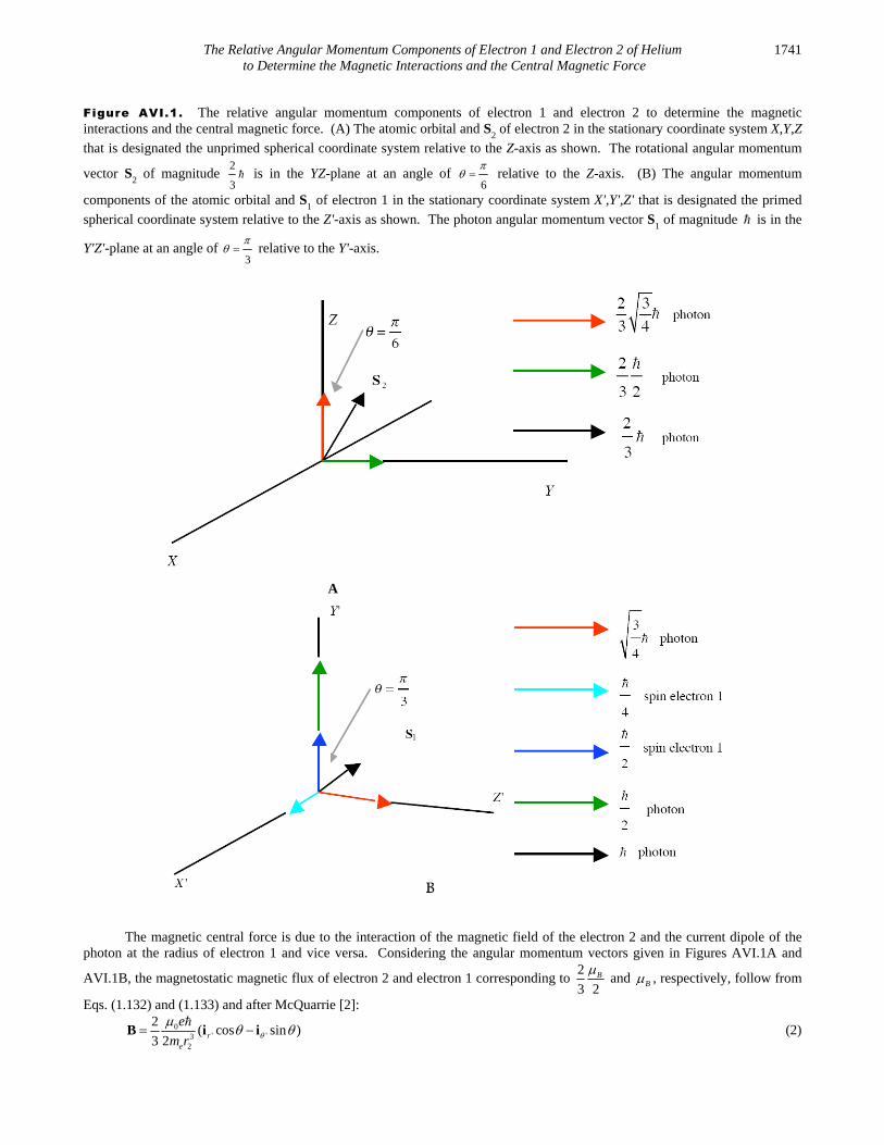
The Relative Angular Momentum Components of Electron 1 and Electron 2 of Helium to Determine the Magnetic Interactions and the Central Magnetic Force
1741
Figure AVI.1. The relative angular momentum components of electron 1 and electron 2 to determine the magnetic interactions and the central magnetic force. (A) The atomic orbital and S
2 of electron 2 in the stationary coordinate system X,Y,Z
that is designated the unprimed spherical coordinate system relative to the Z-axis as shown. The rotational angular momentum
vector S2 of magnitude
2
3 is in the YZ-plane at an angle of
6
relative to the Z-axis. (B) The angular momentum
components of the atomic orbital and S1 of electron 1 in the stationary coordinate system X',Y',Z' that is designated the primed
spherical coordinate system relative to the Z'-axis as shown. The photon angular momentum vector S1 of magnitude is in the
Y'Z'-plane at an angle of 3
relative to the Y'-axis.
A
The magnetic central force is due to the interaction of the magnetic field of the electron 2 and the current dipole of the photon at the radius of electron 1 and vice versa. Considering the angular momentum vectors given in Figures AVI.1A and
AVI.1B, the magnetostatic magnetic flux of electron 2 and electron 1 corresponding to 2
3 2B and B , respectively, follow from
Eqs. (1.132) and (1.133) and after McQuarrie [2]:
0' '3
2
2( cos sin )
3 2 re
e
m r B i i
(2)

Appendix VI 1742
3
( 2cos sin )2 r
e
e
m r B i i
(3)
where 0 is the permeability of free space ( 7 2 4 10 /X N A ) and the coordinates of the magnetic field due to electron 2 acting
on the magnetic moments of electron 1 is designated as the primed system and the magnetic field of electron 1 acting on the magnetic moments of electron 2 is designated as the unprimed system. It follows from Eq. (1.131), the relationship for the Bohr magneton, and relationship between the magnetic dipole field and the magnetic moment m [3] that Eqs. (1.132) and (1.133) are
the equations for the magnetic field due to a magnetic moment of one third of a Bohr magneton, 2
3 2B zm i and one Bohr
magneton, B zm i , respectively, where cos sin z ri i i . The spherical harmonic dipole , sinmY spins about the
S-axis at the angular velocity given by Eq. (1.36). Thus, angular velocity and linear velocity v projections onto each Z(Z')-axis are:
2
2
2 3ˆ
3 4 Zem r
i
(4)
2
2 3sin
3 4em r v i
(5)
'21
3ˆ
4 Zem r
i
(6)
'1
3sin
4em r v i
(7)
The Lorentz force density at each point moving at velocity v given by Eq. (7.10) is
2
24mag
e
r F v B (8)
Substitution of Eqs. (2-3), (5), and (7) into Eq. (8) while maintaining the designation of the coordinates of the magnetic field of electron 2 acting on the magnetic moments of electron 1 as the primed system and the coordinates of the magnetic field of electron 1 acting on the magnetic moments of electron 2 as the unprimed system gives:
0' ' '3
1 2
22 0
32 2
3 2sin cos sin
4 3 2
4 2 3sin 2cos sin
3 4 2
re e
mag
re e
e
m r m re
r e
m r m r
i i i
F
i i i
(9)
As shown in Eqs. (7.16-7.24), the relativistic form of Eq. (9) results in the equivalence of the velocity at the two radii; thus, r1
may be substituted for r2 in the velocity factor of the second term to give:
2 2' ' '0
2 2 32 1 2
22 2' '0
2 2 3 22 1 2
sin cos sin1 2 3
4 2 3 4 sin 2cos sin
sin cos sin1 2 3
4 2 3 4 2sin cos sin
r
mage r
r
e r
e
r r m r
e
r r m r
i i iF
i i i
i i
i i
(10)
The 'ri unit vector is transformed to ri by substituting with 2
in the second term of Eq. (10):
22 2' '0
2 2 32 1 2 2
2 22 2'0
2 2 32 1 2
2 20
2 22 1 2
sin cos sin1 2 32
4 2 3 42sin cos sin
sin cos sin cos1 2 3
4 2 3 4 2sin cos
1
4 2
r
mage
r
r
e
e
e
r r m r
e
r r m r
e
r r m r
i iF
i i
i i
i
'3
2 20
'2 2 32 1 2
2 3sin cos 2sin cos
3 4
1 2 3 1 sin 2 sin 2
4 2 3 4 2
r
re
e
r r m r
i i i
i i i
(11)

The Relative Angular Momentum Components of Electron 1 and Electron 2 of Helium to Determine the Magnetic Interactions and the Central Magnetic Force
1743
The magF i and 'magF i average to zero over the surface for 0 . The relativistic correction given by Eq. (7.23) is based on
quantized-angular-momentum conservation with the emission of a photon. The relativistic correction for the lightlike frame causes the circumferential distances on the surface to dilate to the radial dimension alone as given in the Two-Electron Atoms section. This causes the angular force to vanish since it averages to zero such that only the radial force remains. Since there is no net angular force on the electron, only the resultant radial force need be considered:
2 2
02 2 3
2 1 2
1 2 3
4 2 3 4mag re
e
r r m r
F i
(12)
Eq. (12) may be written in the form
2 2
02 2 3
2 1 2
1 21
4 2 3mag re
es s
r r m r
F i
(13)
where 1/ 2s and 3
( 1)4
s s is the historical designation of the spin-angular momentum magnitude. Then, the balance
between the centrifugal and electric and magnetic forces is given by the Eq. (9.10):
2 2 2 2
3 2 32 2 0 2 2
1 2 1( 1)
4 3 2e
e e
m v es s
r m r n r n m r
(14)
TRIPLET EXCITED STATES WITH = 0 ( 12 11 1s s ns
) For the 0 singlet state, the time-averaged spin angular momentum of electron 2 is zero. The 0 triplet state requires a further excitation to unpair the spin states of the two electrons. The angular momentum corresponding to the excited state is , and the angular momentum change corresponding to the spin-flip is also as given in the Magnetic Parameters of the Electron (Bohr Magneton) section. Then, the triplet state comprises spin interaction terms between the two electrons plus a contribution from the unpairing photon. As shown in the Resonant Precession of the Spin-1/2-Current-Density Function Gives Rise to the Bohr Magneton section, the electron spin angular momentum gives rise to a trapped photon with of angular momentum along an S-axis. Then, the spin state of each of electron 1 and 2 comprises a photon standing wave that is phase-matched to a spherical harmonic source current, a spherical harmonic dipole , sinmY with respect to the S-axis. The dipole spins about the S-
axis at the angular velocity given by Eq. (1.55) with of angular momentum. To conserve angular momentum, electron 2 rotates in the opposite direction about S, the axis of the photon angular momentum due to the spin, and this rotation corresponds
to 2
3 of angular momentum relative to S. The intrinsic spin and photon angular momentum vectors are shown in Figure
AVI.2.
In the stationary coordinate system of electron 2 (denoted by the axes labeled X, Y, and Z in Figure AVI.2A), the 4
of
intrinsic angular momentum is along X, the 2
of intrinsic angular momentum is along Y, and S
3, the photon angular
momentum vector due to spin interaction, is in the YZ -plane at an angle of 3
relative to the Y -axis. The Z -axis projection
of 3S is 3
4 , and the Y -axis projection of 3S is
2
.
Electron 2 is excited by the additional spin-unpairing photon. The angular momentum vector S4 of magnitude in the
XZ-plane is aligned in the plane perpendicular to S3 at an angle of
6
relative to the Z-axis. The Z-axis projection of S4 is
3
4 , and the X-axis projection of S
4 is
2
.
In order to conserve angular momentum, the rotational angular momentum vector of the singlet state S2 is now aligned in
the opposite direction to that of the photonic spin vector 3S . The angular momentum vector S2 of magnitude
2
3 is in the YZ-
plane at an angle of 6
relative to the Z -axis. The Z-axis projection of 2S is 2 3
3 4 , and the Y-axis projection of S
2 is
2
3 2
. Then, the total angular momentum along the Z-axis due to spin, unpairing, and rotation is:

Appendix VI 1744
3 3 2 3 4 3
4 4 3 4 3 4Z Z
S i i (15)
and the total angular momentum along the Y-axis comprising the sum of the initial 2
intrinsic angular momentum, the Y-axis
projection of S3 of
2
, and the Y-axis projection of S
2 of
2
3 2
is:
2 4
2 2 3 2 3 2Z Y
S i i
(16)
In the stationary coordinate system of electron 1 (denoted by the axes labeled X', Y', and Z' in Figure AVI.2B), the 4
of
intrinsic angular momentum is along X', the 2
of intrinsic angular momentum is along 'Y , and the photon angular momentum
vector 1S of magnitude is in the Y'Z'-plane at an angle of 3
relative to the Y'-axis. The Z'-axis projection of 1S is 3
4 ,
and the Y'-axis projection of S1 is
2
.
The torque from the corresponding magnetic moments is given by Eq. (2.65) are balanced in the absence of Larmor precession for the angular momentum projections of electron 2 shown in Figure AVI.2A relative to those of electron 1 shown in
Figure AVI.2B. The superposition of the 4
of intrinsic angular momentum of electrons 1 and 2 along X' and X, respectively,
each with a corresponding magnetic moment of 4
B (Eq. (2.65)) cancel the X-axis projection of S
4 of
2
with a corresponding
magnetic moment of 2
B . The 4
3 2
of total angular momentum of electron 2 along Y gives rise to magnetic field
corresponding to 4
3 2B in the direction of the
3
4 'Z -axis projection of S
1 of electron 1. The
2
of intrinsic angular
momentum of electron 1 along Y' and the Y'-axis projection of S1 of
2
gives rise to a total of with a magnetic field
corresponding to B in the direction of the 4 3
3 4 total Z-axis projection of electron 2.

The Relative Angular Momentum Components of Electron 1 and Electron 2 of Helium to Determine the Magnetic Interactions and the Central Magnetic Force
1745
Figure AVI.2. The relative angular momentum components of electron 1 and electron 2 to determine the magnetic interactions and the central magnetic force. (A) The atomic orbital and S
2, S
3, and S
4 of electron 2 in the stationary coordinate
system X,Y,Z that is designated the unprimed spherical coordinate system relative to the Z-axis as shown. The rotational angular
momentum vector S2 of magnitude
2
3 is in the YZ-plane at an angle of
6
relative to the –Z-axis. S3, the photon angular
momentum vector due to spin interaction, is in the YZ-plane at an angle of 6
relative to the Z-axis. S4, the photon angular
momentum vector due to spin unpairing, is in the XZ-plane at an angle of 6
relative to the Z-axis. (B) The angular
momentum components of the atomic orbital and S1 of electron 1 in the stationary coordinate system X',Y',Z' that is designated
the primed spherical coordinate system relative to the Z'-axis as shown. The photon angular momentum vector S1 of magnitude
is in the Y'Z'-plane at an angle of 3
relative to the Y'-axis.
A

Appendix VI 1746
B
For each electron, the magnetic field corresponding to a magnetic moment of B interacting with an aligned magnetic
momentum of 4 3
3 4 B gives the magnetic force for electron 2 that is twice that of the singlet states. The magnetic central force
is due to the interaction of the magnetic field of electron 2 and the current dipole of the photon at the radius of electron 1 and vice versa. Considering the angular momentum vectors given in Figures AVI.2A and AVI.2B, the magnetostatic magnetic flux
of electron 2 and electron 1 corresponding to 4
3 2B and B , respectively, follow from Eqs. (1.132) and (1.133) and after
McQuarrie [2]:
0' '3
2
4( cos sin )
3 2 re
e
m r B i i
(17)
3
( 2cos sin )re
e
m r B i i
(18)
where 0 is the permeability of free space ( 7 2 4 10 /X N A ) and the coordinates of the magnetic field due to electron 2 acting
on the magnetic moments of electron 1 is designated as the primed system and the magnetic field of electron 1 acting on the magnetic moments of electron 2 is designated as the unprimed system. The angular velocity and linear velocity v projections onto each Z(Z')-axis are:
2
2
4 3ˆ
3 4 Zem r
i
(19)
2
4 3sin
3 4em r v i
(20)
'21
3ˆ
4 Zem r
i
(21)
'1
3sin
4em r v i
(22)
The Lorentz force density at each point moving at velocity v is given by Eq. (8). Substitution of Eqs. (17-18), (20), and (22) into Eq. (8) while maintaining the designation of the coordinates of the magnetic field of electron 2 acting on the magnetic moments of electron 1 as the primed system and the coordinates of the magnetic field of electron 1 acting on the magnetic moments of electron 2 as the unprimed system gives

The Relative Angular Momentum Components of Electron 1 and Electron 2 of Helium to Determine the Magnetic Interactions and the Central Magnetic Force
1747
0' ' '3
1 2
22 0
32 2
3 4sin cos sin
4 3 2
4 4 3sin 2cos sin
3 4 2
re e
mag
re e
e
m r m re
r e
m r m r
i i i
F
i i i
(23)
From Eqs. (10-13), the magnetic force is:
2
2 32 2
4 1( 1)
4 3 2mag re
es s
r n m r F i
(24)
The force balance between the centrifugal and electric and magnetic forces given by Eq. (9.31) is:
2 2 2 2
3 2 32 2 0 2 2
1 4 1( 1)
4 3 2e
e e
m v es s
r m r n r n m r
(25)
SINGLET EXCITED STATES WITH ≠ 0 With 0 , the electron source current in the singlet excited state is the sum of constant and time-dependent functions where the latter, given by Eqs. (1.28-1.29), travels about the Z-axis in the case of electron 2. The corresponding angular momentum along
the rotational axis of 1
superimposes with the projection of the spin angular momentum of 3
4 . The vectors are in
opposite directions in order to conserve angular momentum during excitation. The intrinsic spin and photon angular momentum vectors are shown in Figure AVI.3.
In the stationary coordinate system of electron 2 (denoted by the axes labeled X, Y, and Z in Figure AVI.3A), the 4
of
intrinsic angular momentum is along X , the 2
of intrinsic angular momentum is along –Y, and S
3, the photon angular
momentum vector due to spin interaction, is in the XZ-plane at an angle of 6
relative to the –Z-axis. The Z-axis projection
of S3 is
3
4 , and the X-axis projection of S
3 is
2
. S4, the orbital angular momentum of
1
, is directed along the Z-axis
in the opposite direction of the Z-axis component of S3. Thus, in order to conserve angular momentum, the orbital angular
momentum vector S4 corresponding to the rotational angular momentum vector of the 0 singlet and triplet states is now
aligned in the opposite direction to that of the Z-axis component of the photonic spin vector S3, and the total angular momentum
along the Z-axis due to spin and orbital contributions is:
3
1 4 Z
S i
(26)
In the stationary coordinate system of electron 1 (denoted by the axes labeled X', Y', and Z' in Figure AVI.3B), the 4
of
intrinsic angular momentum is along X', the 2
of intrinsic angular momentum is along Y', and the photon angular momentum
vector S1 of magnitude is in the Y'Z'-plane at an angle of
3
relative to the Y'-axis. The Z'-axis projection of S1 is
3
4 ,
and the 'Y -axis projection of 1S is 2
. 2S , the orbital angular momentum of
1
, is directed along the –Z'-axis in the
opposite direction of the Z-axis component of S1. Thus, in order to conserve angular momentum, the orbital angular momentum
vector S2 is aligned in the opposite direction to that of the Z'-axis component of the photonic spin vector S
1, and the total angular
momentum along the Z'-axis due to spin and orbital contributions is:
'
3
4 1 Z
S i
(27)

Appendix VI 1748
The torque from the corresponding magnetic moments given by Eq. (2.65) are balanced in the absence of Larmor precession for the angular momentum projections of electron 2 shown in Figure AVI.3A relative to those of electron 1 shown in
Figure AVI.3B. The superposition of the 4
of intrinsic angular momentum of electrons 1 and 2 along X' and X, respectively,
each with a corresponding magnetic moment of 4
B (Eq. (2.65)) cancel the X -axis projection of S
3 of
2
with a corresponding
magnetic moment of 2
B . The 2
of total angular momentum of electron 2 along Y gives rise to magnetic field
corresponding to 2
B in the direction of the 3
4 1
total Z-axis projection of electron 1. The 2
of intrinsic angular
momentum of electron 1 along Y' and the Y'-axis projection of S1 of
2
gives rise to a total of with a magnetic field
corresponding to B in the direction of the 3
1 4
total Z-axis projection of electron 2.
Figure AVI.3. The relative angular momentum components of electron 1 and electron 2 to determine the magnetic interactions and the central magnetic force. (A) The atomic orbital and S
3 and S
4 of electron 2 in the stationary coordinate
system X,Y,Z that is designated the unprimed spherical coordinate system relative to the Z-axis as shown. S3, the photon
angular momentum vector due to spin interaction, is in the XZ-plane at an angle of 6
relative to the –Z-axis. S4, the orbital
angular momentum of 1
, is directed along the Z-axis in the opposite direction of the Z-axis component of S3. (B) The
angular momentum components of the atomic orbital and S1 of electron 1 in the stationary coordinate system X',Y',Z' that is
designated the primed spherical coordinate system relative to the Z'-axis as shown. The photon angular momentum vector S1 of
magnitude is in the Y'Z'-plane at an angle of 3
relative to the Y'-axis. S2, the orbital angular momentum of
1
, is
directed along the –Z'-axis in the opposite direction of the Z-axis component of S1.
X
Y
Z
S 4
A
6
S 3
4
2
photon
spin electron 2
spin electron 2
2
S 3
3
4 photon S 3
photon S 3
photon1
S 4

The Relative Angular Momentum Components of Electron 1 and Electron 2 of Helium to Determine the Magnetic Interactions and the Central Magnetic Force
1749
4
2
photon
photon
spin electron 1
spin electron 1
Z'
X'
Y'
3
B
3
4 photon
S 2
photon 1
S 2
S1 S 1
S1 2
S 1
The magnetic central force is due to the interaction of the magnetic field of the electron 2 and the current dipole of the
photon at the radius of electron 1 and vice versa. Considering the angular momentum vectors given in Figures AVI.3A and
AVI.3B, the magnetostatic magnetic flux of electron 2 and electron 1 corresponding to 2
B and B , respectively, follow from
Eqs. (1.132) and (1.133) and after McQuarrie [2]:
0' '3
2
( cos sin )2 r
e
e
m r B i i
(28)
3
( 2cos sin )2 r
e
e
m r B i i
(29)
where 0 is the permeability of free space ( 7 2 4 10 /X N A ) and the coordinates of the magnetic field due to electron 2 acting
on the magnetic moments of electron 1 is designated as the primed system and the magnetic field of electron 1 acting on the magnetic moments of electron 2 is designated as the unprimed system. The angular velocity and linear velocity v projections onto each Z(Z')-axis are:
2
2
3ˆ
1 4 Zem r
i
(30)
2
3sin
1 4em r
v i
(31)
'21
3ˆ
4 1 Zem r
i
(32)
'1
3sin
4 1em r
v i
(33)
The Lorentz force density at each point moving at velocity v is given by Eq. (8). Substitution of Eqs. (28-29), (31), and (33) into Eq. (8) while maintaining the designation of the coordinates of the magnetic field of electron 2 acting on the magnetic moments of electron 1 as the primed system and the coordinates of the magnetic field of electron 1 acting on the magnetic moments of electron 2 as the unprimed system gives
0' ' '3
1 2
22 0
32 2
3sin cos sin
4 1 2
4 3sin 2cos sin
1 4 2
re e
mag
re e
e
m r m re
r e
m r m r
i i i
F
i i i
(34)

Appendix VI 1750
From Eqs. (10-13), the magnetic force is
2
2 32 2
1( 1)
4 2 1mag re
es s
r n m r
F i
(35)
The magnetic force between the two electrons is given by the product of magnetic multipole coefficient ,Ma m given
by Eq. (9.49) and the sum of the relativistically corrected Lorentz force terms due to the spin angular and orbital angular
momenta of 1s s and 1
, respectively:
1/2 2
3
31 1 1 12 ( 1)
2 1 !! 2 2 1mag re
s sn m r
F i
(36)
The force balance between the centrifugal and electric and magnetic forces given by Eq. (9.52) is:
1/22 2 2 2
3 2 32 2 0 2
31 1 1 1 12 ( 1)
4 2 1 !! 2 2 1e
e e
m v es s
r m r n r n m r
(37)
TRIPLET EXCITED STATES WITH ≠ 0 With 0 , the electron source current in the singlet excited state is the sum of orbital and spin components. The
1
of
orbital angular momentum of electron 2 superimposes with the projection of the spin angular momentum that is twice that of the 0 singlet state. The vectors are in opposite directions in order to conserve angular momentum during excitation.
The 0 triplet state requires a further excitation to unpair the spin states of the two electrons. The angular momentum corresponding to the excited state is and the angular momentum change corresponding to the spin-flip is also as given in the Magnetic Parameters of the Electron (Bohr Magneton) section. Then, the triplet state comprises spin interaction terms between the two electrons plus a contribution from the unpairing photon. As shown in the Resonant Precession of the Spin-1/2-Current-Density Function Gives Rise to the Bohr Magneton section, the electron spin angular momentum gives rise to a trapped photon with of angular momentum along an S-axis. Then, the spin state of each of electron 1 and 2 comprises a photon standing wave that is phase-matched to a spherical harmonic source current, a spherical harmonic dipole , sinmY with
respect to the S-axis. The dipole spins about the S-axis at the angular velocity given by Eq. (1.36) with of angular momentum. To conserve angular momentum, the orbital angular momentum is in the opposite direction of each Z-axis component of S, the axis of the photon angular momentum due to spin and the axis of the photon angular momentum due to
unpairing, and the corresponding opposite current rotation corresponds to 1
2 1
of angular momentum relative to each
photon vector S. The intrinsic spin and photon angular momentum vectors are shown in Figure AVI.4.
In the stationary coordinate system of electron 2 (denoted by the axes labeled X, Y, and Z in Figure AVI.4A), the 4
of
intrinsic angular momentum is along X, the 2
of intrinsic angular momentum is along Y, and S
3, the photon angular
momentum vector due to spin interaction, is in the YZ-plane at an angle of 6
relative to the Z-axis. The Z-axis projection of
S3 is
3
4 , and the Y-axis projection of S
3 is
2
.
Electron 2 is excited by the additional spin-unpairing photon. The angular momentum vector 4S of magnitude in the
XZ-plane is aligned in the plane perpendicular to S3 at an angle of
6
relative to the Z-axis. The Z-axis projection of S4 is
3
4 , and the X-axis projection of S
4 is
2
.
In order to conserve angular momentum, the orbital angular momentum vector S2 corresponding to the rotational angular
momentum vector of the 0 singlet and triplet states state is now aligned in the opposite direction to that of the photonic spin

The Relative Angular Momentum Components of Electron 1 and Electron 2 of Helium to Determine the Magnetic Interactions and the Central Magnetic Force
1751
vectors S3 and S4
. S2, the orbital angular momentum of
1
, is directed along the –Z-axis in the opposite direction of the Z-
axis component of S3 and S4
. The total angular momentum along the Z-axis due to spin, unpairing, and orbital components is
3 3 3
24 4 1 4 1Z Z
S i i
(38)
and the total angular momentum along the Y-axis comprising the sum of the initial 2
intrinsic angular momentum and the Y-axis
projection of S3 of
2
is:
2 2 Z Y
S i i (39)
In the stationary coordinate system of electron 1 (denoted by the axes labeled X', Y', and Z' in Figure AVI.4B), the 4
of
intrinsic angular momentum is along X', the 2
of intrinsic angular momentum is along Y', and the photon angular momentum
vector S1 of magnitude is in the Y'Z'-plane at an angle of
3
relative to the Y'-axis. The Z'-axis projection of S1 is
3
4 ,
and the Y'-axis projection of S1 is
2
. Since the
3
4
'Z -axis projection of S
1 is one half that of the Z-axis component of S
3 and
S4, the orbital angular momentum S
2 is
1
2 1
and is directed along the –Z'-axis in the opposite direction of the Z-axis
component of S1. Thus, in order to conserve angular momentum, the orbital angular momentum vector of the triplet state S
2 is
aligned in the opposite direction to that of the Z'-axis component of the photonic spin vector S1, and the total angular momentum
along the Z'-axis due to spin and orbital contributions is
'
3 1
4 2 1 Z
S i
(40)
The torque from the corresponding magnetic moments given by Eq. (2.65) is balanced in the absence of Larmor precession for the angular momentum projections of electron 2 shown in Figure AVI.4A relative to those of electron 1 shown in
Figure AVI.4B. The superposition of the 4
of intrinsic angular momentum of electrons 1 and 2 along X' and X, respectively,
each with a corresponding magnetic moment of 4
B (Eq. (2.65)) cancel the X-axis projection of S
4 of
2
with a corresponding
magnetic moment of 2
B . The of total angular momentum of electron 2 along Y gives rise to magnetic field corresponding
to B in the direction of the 3 1
4 2 1
total Z-axis projection of electron 1. The 2
of intrinsic angular momentum of
electron 1 along Y' and the Y'-axis projection of S1 of
2
gives rise to a total of with a magnetic field corresponding to B in
the direction of the 3
24 1
total Z-axis projection of electron 2.

Appendix VI 1752
Figure AVI.4. The relative angular momentum components of electron 1 and electron 2 to determine the magnetic interactions and the central magnetic force. (A) The atomic orbital and S
2, S
3, and S
4 of electron 2 in the stationary coordinate
system X,Y,Z that is designated the unprimed spherical coordinate system relative to the Z-axis as shown. The orbital angular
momentum vector S2 of magnitude
1
is along the –Z-axis. S3, the photon angular momentum vector due to spin
interaction, is in the YZ-plane at an angle of 6
relative to the Z-axis. S4, the photon angular momentum vector due to spin
unpairing, is in the XZ-plane at an angle of 6
relative to the Z-axis. (B) The angular momentum components of the atomic
orbital and S1 of electron 1 in the stationary coordinate system X',Y',Z' that is designated the primed spherical coordinate system
relative to the Z'-axis as shown. The photon angular momentum vector S1 of magnitude is in the Y'Z'-plane at an angle of
3
relative to the Y'-axis. S2, the orbital angular momentum of
1
2 1
, is directed along the –Z'-axis in the opposite
direction of the Z-axis component of S1.

The Relative Angular Momentum Components of Electron 1 and Electron 2 of Helium to Determine the Magnetic Interactions and the Central Magnetic Force
1753
The magnetic central force is due to the interaction of the magnetic field of the electron 2 and the current dipole of the
photon at the radius of electron 1 and vice versa. Considering the angular momentum vectors given in Figures AVI.4A and AVI.4B, the magnetostatic magnetic flux of electron 2 and electron 1 corresponding to B and B , respectively, follow from
Eqs. (1.132) and (1.133) and after McQuarrie [2]:
0' '3
2
( cos sin )re
e
m r B i i
(41)
3
( 2cos sin )2 r
e
e
m r B i i
(42)
where 0 is the permeability of free space ( 7 2 4 10 /X N A ) and the coordinates of the magnetic field due to electron 2 acting
on the magnetic moments of electron 1 is designated as the primed system and the magnetic field of electron 1 acting on the magnetic moments of electron 2 is designated as the unprimed system. The angular velocity and linear velocity v projections onto each Z(Z') -axis are:
2
2
3ˆ 2
4 1 Zem r
i
(43)
2
32 sin
4 1em r
v i
(44)
'21
3 1ˆ
4 2 1 Zem r
i
(45)
'1
3 1sin
4 2 1em r
v i
(46)
The Lorentz force density at each point moving at velocity v is given by Eq. (8). Substitution of Eqs. (41-42), (44), and (46) into Eq. (8) while maintaining the designation of the coordinates of the magnetic field of electron 2 acting on the magnetic moments of electron 1 as the primed system and the coordinates of the magnetic field of electron 1 acting on the magnetic moments of electron 2 as the unprimed system gives

Appendix VI 1754
0' ' '3
1 2
22 0
32 2
3 1sin cos sin
4 2 1
4 32 sin 2cos sin
4 1 2
re e
mag
re e
e
m r m re
r e
m r m r
i i i
F
i i i
(47)
From Eqs. (10-13), the magnetic force is
2
2 32 2
12 ( 1)
4 2 1mag re
es s
r n m r
F i
(48)
The magnetic force between the two electrons is given by the product of magnetic multipole coefficient ,Ma m given
by Eq. (9.49) and the sum of the relativistically corrected Lorentz force terms due to the spin angular and orbital angular
momenta of 1s s and 1
, respectively:
1/2 2
3
31 1 1 12 2 ( 1)
2 1 !! 2 2 1mag re
s sn m r
F i
(49)
The force balance between the centrifugal and electric and magnetic forces given by Eq. (9.63) is
1/22 2 2 2
3 2 32 2 0 2
31 1 1 1 12 2 ( 1)
4 2 1 !! 2 2 1e
e e
m v es s
r m r n r n m r
(50)
REFERENCES 1. J. D. Jackson, Classical Electrodynamics, Second Edition, John Wiley & Sons, New York, (1975), pp. 236-240, 601-608,
786-790. 2. D. A. McQuarrie, Quantum Chemistry, University Science Books, Mill Valley, CA, (1983), pp. 238-241. 3. J. D. Jackson, Classical Electrodynamics, Second Edition, John Wiley & Sons, New York, (1975), p. 178.

ABOUT THE AUTHOR
Randell L. Mills received a Bachelor of Arts Degree in chemistry, summa cum laude and Phi Beta Kappa from Franklin & Marshall College and a Doctor of Medicine Degree from Harvard Medical School with a concentration on technology while also studying electrical engineering at the Massachusetts Institute of Technology. He is the Founder and President of Brilliant Light Power, Inc., based in the Princeton, New Jersey area that is developing technologies based on novel hydrogen chemistry. He has authored or co-authored over a hundred (100) articles and a book in this field. He is also active in a number of other areas of technology. He has received or filed patent applications in the following areas: (1) hydrino/SunCell power source; (2) computational chemical design technology; (3) magnetic resonance imaging; (4) Mossbauer cancer therapy; (5) Luminide class of drug delivery molecules; (6) genomic sequencing method, (7) artificial intelligence, and (8) fifth force technology. He is a member of the American Chemical Society.
ACKNOWLEDGMENTS Special thanks to H. Hlucha for reviewing the mathematics regarding spin, T. Bujnak, for writing the normalization algorithm, and to Dr. J. Farrell, Dr.-Ing. Günther Landvogt, and Dr. R. Engelmann for comments on past drafts of this manuscript, to B. Holverstott for work on the figures, and to the BlackLight Power, Inc. shareholders who made this work possible by their financial and moral support. Gratitude is also due to Beata Stepien, Samantha Ash, and John Lotoski for the arduous task of organizing this tome for publication.

Dr. Randell Mills holds a Doctor of Medicine degree from Harvard, a BA degree in Chemistry from Franklin and Marshall College, and studied Electrical Engineering at MIT. He is President, Chairman and CEO of BlackLight Power, Inc.
Dr. Mills has advanced the field generally known as Quantum Mechanics by deriving a new atomic theory of Classical Physics (CP) from first principles, which unifies Maxwell’s Equations, Newton’s Laws, and Einstein’s General and Special Relativity. The central feature is that physical laws hold over all scales, from the scale of subatomic particles to that of the cosmos.
From two basic equations, the key building blocks of organic chemistry have been solved, allowing the true physical structure and parameters of an infinite number of organic molecules up to infinite length and complexity to be obtained. These equations were also applied to bulk forms of matter, such as the allotropes of carbon, the solid bond of silicon and the semiconductor bond; as well as fundamental forms of matter such as the ionic bond and the metallic bond; and major fields of chemistry such as that of silicon, tin, aluminum, boron, coordinate compounds and organometallics.
“Mills’ theory explains the answers to some very old scientific questions, such as ‘what happens to a photon upon absorption’ and some very modern ones, such as ‘what is dark matter.’ ...Lastly, Mills has made an extremely important contribution to the philosophy of science. He has reestablished cause and effect as the basic principle of science.” Dr. John J. Farrell, former Chair of the Dept. of Chemistry, Franklin & Marshall College “Mills’ ingenious way of thinking creates in different physical areas astonishing results with fascinating mathematical simplicity and harmony. And his theory is strongly supported by the fact that nearly all these results are in comfortable accordance with experimental findings, sometimes with breathtaking accuracy.” Dr Günther Landvogt, Retired Scientist, Philips Research Lab “Dr. Mills has apparently completed Einstein’s quest for a unified field theory… without largesse from the US Government, and without the benediction of the US scientific priesthood.”
Shelby T. Brewer, former Assistant Secretary of Energy, former CEO of ABB Combustion Engineering, MS/Ph.D. MIT - Nuclear Engineering.
“Mills proposes such a basic approach to quantum theory that it deserves considerably more attention from the general scientific community than it has received so far. The new theory appears to be a realization of Einstein’s vision and a fitting closure of the “Quantum Century” that started in 1900...”
Dr. Reinhart Engelmann, Professor of Electrical Engineering, Oregon Graduate Institute of Science and Technology
Further, the Schwarzschild Metric is derived by applying Maxwell’s Equations to electromagnetic and gravitational fields at particle production. This modifies General Relativity to include the conservation of spacetime and gives the origin of gravity, the families and masses of fundamental particles, the acceleration of the expansion of the Universe (predicted by Dr. Mills in 1995 and since confirmed experimentally), and overturns the Big Bang model of the origin of the Universe.
Dr. Randell Mills holds a Doctor of Medicine degree from Harvard, a BA degree in Chemistry from Franklin and Marshall College, and studied Electrical Engineering at MIT. He is President, Chairman and CEO of Brilliant Light Power, Inc.
Quantum Mechanics has remained mysterious to all who have encountered it. Whereas Schrödinger postulated a boundary condition Ψ → 0 as r → ∞ resulting in a purely mathematical model of the hydrogen atom, CP was derived from known physics, i.e. Maxwell’s Equations. Under special conditions, an extended distribution of charge may accelerate without radiating energy. This leads to a physical model of subatomic particles, atoms, and molecules. Equations are closed-form solutions containing fundamental constants only and agree with experimental observations.