The government intervention in the pricing of wheat in the United ...
64
Atlanta University Center DigitalCommons@Robert W. Woodruff Library, Atlanta University Center ETD Collection for AUC Robert W. Woodruff Library 7-1-1985 e government intervention in the pricing of wheat in the United States and its global effects Solomon Odenore Usianeneh Atlanta University Follow this and additional works at: hp://digitalcommons.auctr.edu/dissertations Part of the Economics Commons is esis is brought to you for free and open access by DigitalCommons@Robert W. Woodruff Library, Atlanta University Center. It has been accepted for inclusion in ETD Collection for AUC Robert W. Woodruff Library by an authorized administrator of DigitalCommons@Robert W. Woodruff Library, Atlanta University Center. For more information, please contact [email protected]. Recommended Citation Usianeneh, Solomon Odenore, "e government intervention in the pricing of wheat in the United States and its global effects" (1985). ETD Collection for AUC Robert W. Woodruff Library. Paper 1485.
Transcript of The government intervention in the pricing of wheat in the United ...
Atlanta University CenterDigitalCommons@Robert W. Woodruff Library, AtlantaUniversity Center
ETD Collection for AUC Robert W. Woodruff Library
7-1-1985
The government intervention in the pricing ofwheat in the United States and its global effectsSolomon Odenore UsianenehAtlanta University
Follow this and additional works at: http://digitalcommons.auctr.edu/dissertations
Part of the Economics Commons
This Thesis is brought to you for free and open access by DigitalCommons@Robert W. Woodruff Library, Atlanta University Center. It has beenaccepted for inclusion in ETD Collection for AUC Robert W. Woodruff Library by an authorized administrator of DigitalCommons@Robert W.Woodruff Library, Atlanta University Center. For more information, please contact [email protected].
Recommended CitationUsianeneh, Solomon Odenore, "The government intervention in the pricing of wheat in the United States and its global effects"(1985). ETD Collection for AUC Robert W. Woodruff Library. Paper 1485.
ABSTRACT
DEPARTMENT OF ECONOMICS
USIANENEH5 SOLOMON ODENORE B.S.. Bowling Green State University, 1983
i" t.hB Pricing of Wheat in the United States
and Its Global Effects
Adviser: Dr. Fred Boadu
Thesis dated July 1985
This thesis was concerned with a quantification of the effects of
a government intervention in the pricing of wheat in the United States.
First, standard partial equilibrium comparative static analysis in the
Marshallian economic surplus framwork-welfare theory-was used to
calculate the net social loss in consumption, net social loss in
production, welfare gain of producers, and welfare gain of consumers.
Second, a Marshallian demand function-theory of consumer behavior-
was employed through the use of ordinary least squares techniques to
estimate the parameters in the aforementioned welfare theory. Lastly,
partial equilibrium market model-a linear model of price determination
in an isolated market-was used to show the diagrammatic effects of
equilibrium price.
It was found in this study that government intervention in the
pricing of wheat has a negative rate of protection on the domestic
consumption of wheat, i.e., the quantity of wheat consumed in this
country is substantial less than what it wou!d have been in the absence
of price distortions.
THE GOVERNMENT INTERVENTION IN THE PRICING OF WHEAT
IN THE UNITED STATES AND ITS GLOBAL EFFECTS
A THESIS
SUBMITTED TO THE FACULTY OF ATLANTA UNIVERSITY IN
PARTIAL FULFILLMENT OF THE REQUIREMENT FOR THE
DEGREE OF MASTERS OF ARTS
BY
SOLOMON 0. USIANENEH
DEPARTMENT OF ECONOMICS
ATLANTA, GEORGIA
JULY 1985
DEDICATION
This thesis is dedicated to my lovely wife Bernadine, for her support,
patience, and kindness. Her belief in a beautiful tomorrow has become my
daily source of strength; thus, I am able to do the things I do.
ACKNOWLEDGEMENT
The accomplishment of the task of writing this thesis would have
not been successful without the professional guidance of Dr. Fred Boadu.
I gratefully acknowledge and wholeheartedly appreciate his constructive
criticisms and assistance.
ii
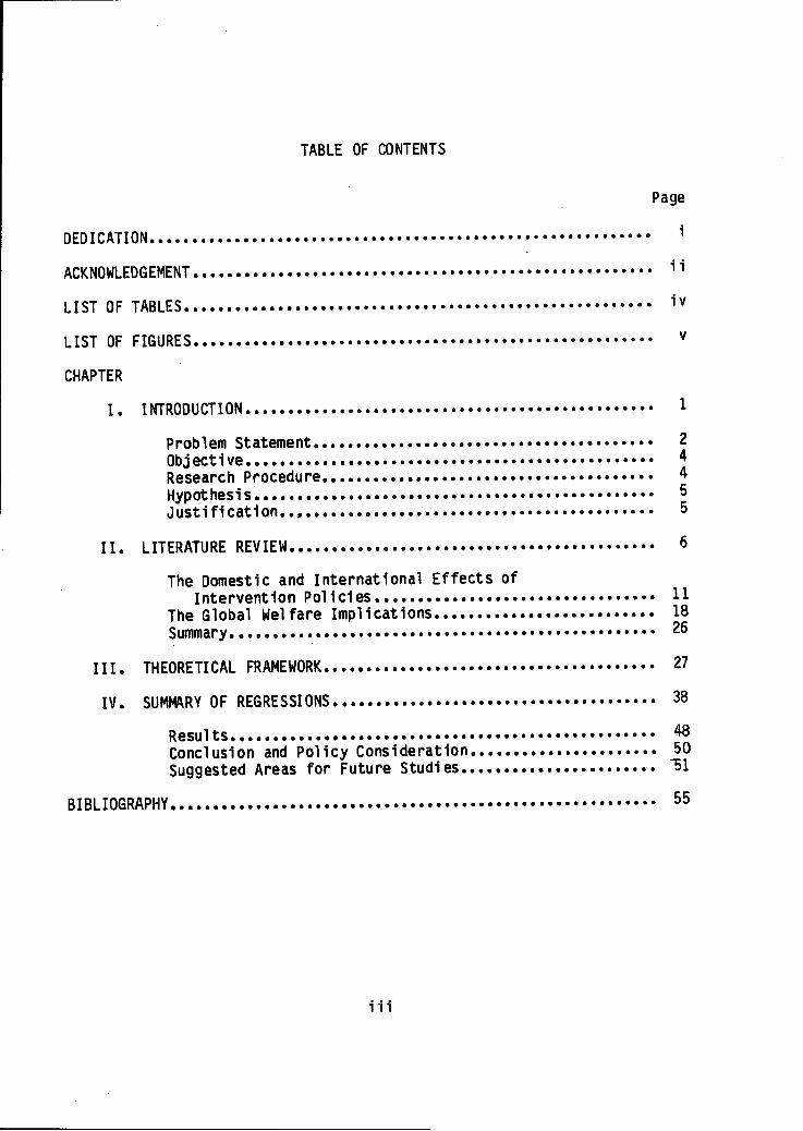
TABLE OF CONTENTS
Page
DEDICATION i
ACKNOWLEDGEMENT 11
LIST OF TABLES iv
LIST OF FIGURES v
CHAPTER
I. INTRODUCTION 1
Problem Statement 2Obj ect i ve 4Research Procedure 4Hypot hes i s 5J ust i fi cat i on.., 5
II. LITERATURE REVIEW 6
The Domestic and International Effects of
Intervention Policies 11The Global Welfare Implications 18
Summary 26
III. THEORETICAL FRAMEWORK 27
IV. SUMMARY OF REGRESSIONS 38
Resul ts 48Conclusion and Policy Consideration 50Suggested Areas for Future Studies "51
BIBLIOGRAPHY 55
iii
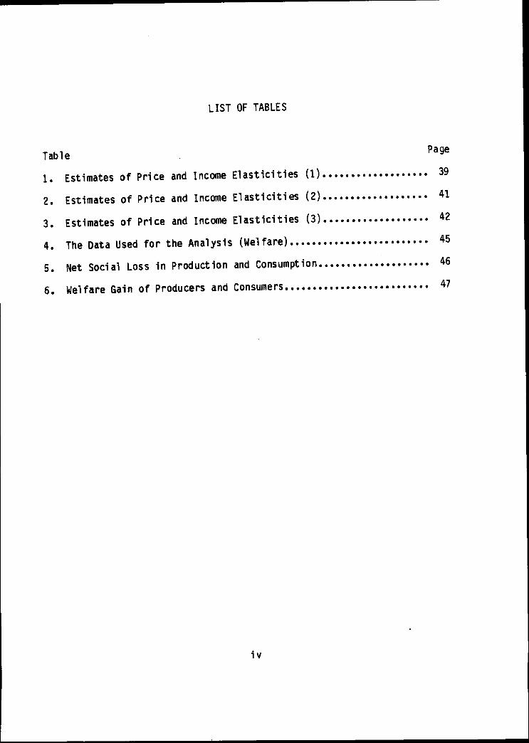
LIST OF TABLES
Table . Page
1. Estimates of Price and Income Elasticities (1) 39
2. Estimates of Price and Income Elasticities (2) 41
3. Estimates of Price and Income Elasticities (3) 42
4. The Data Used for the Analysis (Welfare) 45
5. Net Social Loss in Production and Consumption 46
6. Welfare Gain of Producers and Consumers 47
iv
LIST OF FIGURES
Figure
1. International Commodity Agreement 7
2. Partial Equilibrium Market Model 32
3. An Increase in Exogenous Parameter A 33
4. An Increase in Exogenous Parameter P 34
5. An Increase in Exogenous Parameter a 35
6. An Increase in Exogenous Parameter 6 36

CHAPTER I
INTRODUCTION
Price instability in the agricultural sector of the United States
has been an issue of long concern to farmers, economists and government
officials, and over the years, a great deal of effort has been made by
many economists to explain its effects. The focus has been on who loses
from these price changes.
Instability originates basically from two sources, namely, real and
policy induced ones.1 Natural random factors influence both supply and
demand of agricultural commodities. Production of farm products can be
affected by weather, technological change, and in some cases, by input
variability. Demand, on the other hand, varies in most cases, due to
fluctuating income and taste changes.
In response to the problem of price instability, one observes an
increase in legislation by authorities designed to protect the farm sector.
These range from "set-aside" schemes, to income support-deficiency payments,
and in some cases, direct subsidies are given to farmers. "In the United
States, target prices are established and farmers participating in "set-
aside" schemes receive deficiency payment amounting to the difference
between the target prices and the average market prices."2 Products under
ID. Heien, "Price Determination Process for Agricultural Sector Models,"American Journal of Agricultural Economics, 59 (1977), p. 126.
2d. G. Johnson, "World Agriculture, Commodity Policy, and PriceVariability." American Journal of Agricultural Economics, 56 (1975), p. 823.
-1-
-2-
this scheme are mainly foodgratns and feedgrains.3
In general, government intervenes in agricultural price-setting
mechanism in many different ways and for assorted reasons. For example,
export taxes on agricultural products provide government revenue and
help keep domestic prices low; and vary significantly, the authorities
provide these "set-aside" schemes, income support-deficiency payments
programs, and subsidies as measures to prevent competition from other
countries.
Problem Statement
Many countries—industrialized and developing—engage in protectionsim
as a tool against foreign competition even though it is well documented
that such practices led to price instability at the world market.4
Johnson, examining the International Wheat Agreement signed in
Washington on March 23, 1949-an agreement that fixed the price and the
quantity of wheat to be imported and exported—, stressed the problem
that such procedure creates. He has argued that such action, which is
against free trade, will increase fluctuations of wheat prices at world
market.5 There is, however, a body of literature that corroborates this
3d. G. Johnson, "World Agriculture, Commodity Policy, and PriceVariability," American Journal of Agricultural Economics, 56 (19/5). P»
4s. Y. Shei and R. L. Thompson, "The Impact of Trade Restrictions onPrice Stability in the World Wheat Market," American Journal of AgriculturalEconomics, 59 (1977), p. 629.
5h G. Johnson, "The Destabilizing Effect of International CommodityAgreements on the Prices of Primary Products," The Economic Journal, 3
(1950), p. 626.
-3-
view, namely, the more the degree of protectionism, the more the violent
fluctuations in prices at the world market.6
Bale and Lutz, addressing the distortions of prices of farm products
by government authorities, contend that such measure is disadvantageous
to the farm sector of the exporting country in terms of the realization of
full potential output.7
Wheat is a major exportable foodgrain of this country, and over the
years the quantities exported have continued to increase from 30,987 in
1979 to 48,011 in 1982 (in '000 metric tons).8
In recent years, it has also become an instrument used by government
authorities to achieve political objectives. This problem was manifested
during the Jimmy Carter Administration when an embargo was placed on the
sale of wheat to the Soviet Union, and was considered a problem because
the Soviet Union is a major market for wheat from this country.
The expanded use of economic sanctions in the world today suggest
that studies are needed that will allow us to predict future consequences.
Very little literature exists on the wheat market. This study is therefore
concerned with wheat market from the point of views of economic sanctions
6s. Y. Shei and R. L. Thompson, "The Impact of Trade Restrictions onPrice Stability in the World Wheat Market," American Journal of AgriculturalEconomics, 59 (1977), p. 632.
7M. D. Bale and E. Lutz, "Price Distortions in Agricultural and TheirEffects: An International Comparison." American Journal of Agricultural
Economics, 63 (1981), p. 21.
8world Wheat Statistics, International Wheat Council, London, 1984.
-4-
and protectionism, and attempts to provide empirical and quantified
evidence on the consequences of the latter.
Objective
The fundamental objective of this study is to evaluate the effects of
government intervention policies on the pricing of wheat in the United
States. This will be achieved through the following.
1) Identifying and quantifying various measures of consumer welfare,
including net social loss in production.
2) Measuring the parameters in the consumer welfare analysis by
estimating demand as a function of prices and income.
3) And using the results in (1) and (2) above to explain the domestic
and international ramifications.
Research Procedure
This study will begin with a detail review of the relevant literature
related to government intervention on the pricing policies in the United
States. This will cover historical perspective of protectionism, the
international and domestic effects, and the global welfare implications.
Based on the review, the important factors operating in the United
States and the world wheat market will be identified. The interactions
between the factors will be expressed in mathematical terms and estimated.
One of the postulates that will be made in this study is that world
price is equilibrium price. Mathematical and diagrammatic analysis will
-5-
be provided to show the effect of equilibrium price on the quantity of
wheat in this country.
Finally, the policy implications of all the results of the study will
be emphasized.
Hypothesis
Although government intervention in the pricing of wheat in this
country is of immense advantage to the farmers, it is undesirable in terms
of global welfare.
Justification
This study will make evident the dominant role that price plays in
the wheat market. It will also show that government distortions of wheat
prices result in a drastic reduction of the domestic consumption of wheat
in this country. The empirical evidence is designed to aid policy makers
towards formulating legislations that are prudent for the farm sector.
CHAPTER II
LITERATURE REVIEW
The literature review is divided into three sections: First, the
historical perspective of protectionism of wheat prices is traced; second,
the recent studies on this question with emphasis on international and
domestic effects are evaluated; and third, the global welfare implications
are given a detail consideration.
Johnson (1950), discussed the stated objectives of the International
Wheat Agreement signed in Washington on March 23, 1949—to assure supplies
of wheat to importing countries and markets for wheat to exporting countries
at equitable and stable prices.9 "These objectives were to be secured by
an agreement between the major importing and exporting countries fixing a
maximum quantity of wheat which the importing countries may be required
to buy from the exporting countries at an agreed minimum price, and which
the exporting countries may be required to sell to the importing countries
at an agreed maximum price."10
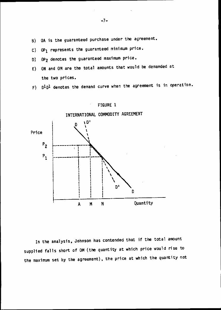
He represented diagrammatically the effect of the agreement on the
demand for the commodity as shown in Figure 1.
A) DO represents the demand curve as it would be in the absence of
any agreement.
9H. 6. Johnson, "The Destabilizing Effect of International CommodityAgreement on the Prices of Primary Products," The Economic Journal, 3 (1950),
p. 627.
10lbi-d.
-6-
-7-
B) OA is the guaranteed purchase under the agreement.
C) OPi represents the guaranteed minimum price.
D) OP2 denotes the guaranteed maximum price.
E) ON and OM are the total amounts that would be demanded at
the two prices.
F) DlDl denotes the demand curve when the agreement is in operation.
Price
FIGURE 1
INTERNATIONAL COMMODITY AGREEMENT
D
Quantity
In the analysis, Johnson has contended that if the total amount
supplied falls short of OM (the quantity at which price would rise to
the maximum set by the agreement), the price at which the quantity not
-8-
covered by the agreement would be higher than the price which would have
cleared the total supply if there had been no agreement. Similarly, the
opposite is true when the amount supplied exceeds ON. Thus it became
obvious that unless quantity variations remain within the OM-ON, and price
variations remain within the OPi - OP2 in which case the agreement would
have no effect on the market. The effect of the agreement would be to
increase fluctuations in prices.
In general therefore, it would seem that an agreement of the Interna
tional Wheat Agreement type would tend to make fluctuations in price more
violent than they would otherwise be.
It is interesting to note that Johnson successfully made the point
about the agreements and how they would increase fluctuations in prices.
However, there was nothing in his article that suggested an alternative.
It was in an attempt to find a workable model that the concept of duopoly
was developed.
McCalla (1966) has considered the market for wheat as a duopoly.11
He argued that only the United States and Canada possessed facilities
necessary to hold the stocks required to exert market power. He defined
market power as the willingness and ability to hold stocks.
He developed a model of duopoly pricing, and it was concerned with
pricing along the residual demand curve facing the duopolists. This he
A. F. McCalla, "A Duopoly Model of World Wheat Pricing," Journal of
Farm Economics, 58 (1966), pp. 711-727.
-9-
obtained by subtracting the supply curves of competing exporters and
producers from the world demand curve.
The point should be made that the results reached by McCalla in his
analysis can only be explained in line with the assumptions he made.
A) He assumed that wheat is a homogeneous commodity.
B) Each seller is aware of how the other will react to his own actions,
C) There is a price leadership and Canada 1s the leader.
D) There is a maximum price above which the second seller will not
follow the leader.
E) The leader has some minimum quantity he must sell and some
minimum price which he would rather hold than sell.
F) Both sellers wish to maximize exports.
What is apparent here is that these assumptions defined a set of
prices and quantities in which a solution was obtained. Based on this
analysis, it was McCalla's contention that because of the market power
possessed by Canada and the United States, the price formation in the
world wheat market would largely be determined by them.
This view contrasts with that of Alaouze, Watson and Sturgess
(1978) ,12 who rejected the concept of duopoly pricing as presented by
McCalla. They argued, first, that there was severe contraction in the
demand facing the duopolists, and it could lead to a breakdown of the
12c. M. Alaouze; A. S. Watson; and N. H. Sturgess, "Oligopoly Pricingin the World Wheat Market," American Journal of Agricultural Economics, 60
(1978), pp. 173-185.
-10-
duopoly. Second, an increase in the exportable surplus of one of the
suppliers would have a destabilizing influence on the duopoly. And lastly,
they argued that when duopoly pricing is consistently followed, the total
market share of the duopolists could not be maintained. A shift in the
residual demand curve toward the price axis, other things being equal,
could distort the market shares of the duopolists.
The authors, diagrammaticallly represented a triopoly model that
included the United States, Canada and Australia, and argued that this
formation was the only way the market shares of the duopolists could be
maintained. The inclusion of Australia—the third largest wheat exporter—
in the arrangement would render the possible shifts in the demand curve of
no effect.
The authors maintained that triopoly would enable the three major
exporters of wheat to retain their market shares and consequently allowed
them to determine the world wheat prices.
Carter and Schmitz (1979) disagreed with Alaouze, Watson and
Sturgess, and McCalla on the concepts of triopoly pricing and duopoly
pricing respectively.13 The major thrust of these concepts was that price
formation in the world wheat market was largely determined by the major
exporters. Carter and Schmitz argued that in light of the trade restric
tions that have been set up by the major wheat importers in the interna-
13c. Carter and A. Schmitz, "Import Tariffs and Price Formation inthe World Wheat Market," American Journal of Agricultural Economics, 61
(1979), pp. 517-521.
-11-
tional market, the effect of a duopoly or triopoly arrangement was
relatively minor. They maintained that world wheat prices are determined
by the major wheat importers. "It is the restrictive policies of the
importers (whether consciously or not) that are likely to result in a
welfare gain to importing countries greater than under free trade."1
The authors combined graphical analysis—optimum tariff solutions--
which were estimates, with actual price and compared them.
They recognized that the structure of the wheat market was more
complex than depicted in their analysis, but stressed that market power
on the part of importers of wheat was greater than the power attributed
to exporters by previous researchers.
This author accepts as true the key point made in the articles by
Alaouze, Watson and Sturgess, and McCalla, namely, that world wheat prices
are determined by the major wheat exporters. In fact, this point has to
hold true in light of the central premise of this study and the postulate
made earlier.
The Domestic and International Effects of Intervention Policies
In order to balance the very many areas that have to be covered in
this study, the international and domestic ramifications of protectionism
are considered.
14C. Carter and A. Schmitz, "Import Tariffs and Price Formation inthe World Wheat Market," American Journal of Agricultural Economics, 61
(1979), p. 519.
-12-
Bale and Lutz (1981) analyzed the effects of agricultural policies
in industrialized nations on their domestic economies, the world commodity
markets, and developing countries.15 They relied heavily on diagrammatic
representations to show that all the real and monetary effects of agricul
tural protectionism depended on the size of the tariff as well as on
supply and demand elasticities.
These graphs, first, depicted a situation of price protection both
in importing and exporting regions. Second, price distortions in a two-
region world model—importing and exporting—were represented. And
finally, transmission of supply instability due to price fixing was brought
to bear in the analysis.
It was the view of the authors that the argicultural protection
policies used in industrialized nations maintain output in inefficient
industries (as judged by world prices). The policies prohibit trade from
developing countries and create price instability at world market.
Finally, they stressed that agricultural protectionism in industrialized
countries is one of the major causes of mi sal located resources use.
In a more defined terms, using specific products, the authors went
ahead and compared price distortions between developed countries and
developing nations.
15m. D. Bale and E. Lutz, "Agricultural Protectionism in IndustrialNations and Its Global Effects: A Survey of Issues," World Bank Staff
Working Paper, No. 248.

-13-
Bale and Lutz (1981) discussed government intervention in the deter
mination of agricultural product prices.16 A comparison was made between
Japan, West Germany, France, and Great Britain, and Thailand, Egypt,
Argentina and Pakistan.
The real effects of agricultural price distortions were analyzed
using nominal protection coefficients. This was used to measure the
disparity between domestic output prices and world prices. The authors
also calculated:
- the change in rural employment;
- welfare gain of producers;
- the change in government revenue;
- welfare gain of consumers;
- net social loss in consumption;
- the change in foreign exchange earnings; and
- net social loss in production.
It was the contention of the authors that as a result of price
distortion, the levels of agricultural production in industrialized nations
were higher than they would be without intervention, whereas agricultural
output in developing countries was significantly smaller than what it
would be in the absence of distortions. The results also showed that
developing countries consume more and developed countries consume less
than they would in the absence of price intervention measures. In general,
16m. D. Bale and E. Lutz, "Price Distortions in Agriculture and Their
Effects: An International Comparison," American Journal of Agricultural
Economics, 63 (1981), pp. 8-21.
-14-
they found that the pricing policies caused a reduction in the exports
of developing countries, and a lessening of imports by the industrialized
nations.
The authors have maintained that because "incorrect" price signals
are being given to farmers, full potential in terms of allocation,
production, and consumption was not being realized.
The authors once again considered the effects of specific trade
intervention policies in importing and exporting countries. Bale and
Lutz (1979) examined the effects of different trade intervention
policies on international price instability.17
They worked with a two-region world model with one commodity, linear
supply and demand functions and additive random disturbances. The variance
in the world market price was taken as the standard against which variances
resulting from different forms of price intervention either by the
exporting or the importing country were compared.
It was calculated that a specific tariff imposed by the importing
country region would lower the foreign price and raise the domestic price,
but would have no effect on price variability in either of the two regions.
On the other hand, an ad valorem tariff imposed by the importing region
would increase the domestic price variance, while the price fluctuations
in the exporting region are reduced. A fixed quota effectively would
17M. D. Bale and E. Lutz, "The Effects of Trade Intervention onInternational Price Instability," American Journal of Agricultural Economics,
61 (1979), pp. 512-516.
-15-
separate the two regions so that no instability is transmitted from one
region to the other. By price fixing all domestically created instability
is exported.
They also considered a case where domestic producers in the importing
region are guaranteed a constant market share, i.e., the import quota is
a constant share of total domestic consumption. Such measure resulted in
the transmission of instability from the exporting to the importing region.
The resulting price variance in the importing region would exceed both the
free-trade and no-trade cases.
It was their contention, however, that the quantitative results
depended on the slopes of the supply and demand functions as well as the
size of the demand and supply disturbances.
Using mathematical analysis, with specific assumptions, Bhagwati
(1974) elaborated on how instability is transmitted from one country to
the other.*8 The analysis was concerned with an evaluation of trade inter
vention by authorities through price-fixing.
He used a two-country, one commodity, equilibrium model of trade to
show that price instability generated by random supply fluntuations in the
importing country can be simplified through price-fixing.
The demand in Country 1 and 2 was given by:
di = a-| - b^P + 6 i
i = 1, 2 and supply was given by Si = a ^ + e iP + e ^
18A. Bhagwati, "The Effects of Trade Interventions," The Economic
Journal, 24 (1974), p. 212.
-16-
i = 1, 2, where: d-j is demand in country i; Si is supply in Country i;
and P is price. The terms ai.bi.oi, &i are fixed parameters and ^ and
ei denotes random variables distributed as N (0,cr~<5i ) and (0,°- e^ )i
respectively. Under free trade, aggregate excess demand is zero, i.e.,
s di - z Si = 0
i i
The equilibrium price was found to be:
Pw = £ ai - a i + 6 i - ei / bi + B ii
and the variance of the free trade market price became:
°~~ Pw = l °~~ 5. + JJ~ e1 / (bi + Bi)2,
provided that $i and e i are distributed independently.
If the price in the importing country is fixed atF2» tne equilibrium
price in the exporting country becomes:
i
1 ■ 1, 2, and the price variance is
^~ P = °~ 6i + °" 62 + °" E2 + ^~ e2 ' (bl + h)Z
It was the contention of the author that because of the result of
price variance, as shown above, the instability in the improving country
is thus exported to the exporting country. He maintained that governments
-17-
seem interested in price stability, particularly for agricultural commodities.
Yet they are interested primarily in internal stability rather than in global
stability.
Still on the same question of price variability at the international
market, Shei and Thompson (1977) devised a simulation to show how different
regional policies affect the world market price.19
A thirteen-region quadratic programming model of world wheat trade
was utilized to simulate the effects of unanticipated quantity changes on
prices in the world wheat market. This simulation was done under different
degrees of trade restrictions.
Three scenarios characterized by different numbers of regions were
specified. These were the regions that permit price signals from inter
national markets.
As the number of countries whose wheat trade is price responsive
increases in the simulation, the percentage change in world price becomes
smaller. This was in response to a shock such as the United States1 export
control and unanticipated external factors.
It was the view of the authors that greater world market price
variability results as more countries prevent world price signals from
being reflected across their borders.
In order to provide some empirical evidence on the factors that create
instability at the world market, Zwart and Meike (1979), evaluated the
19S. Y. Shei and R. L. Thompson, "The Impact of Trade Restrictions onPrice Stability in the World Wheat Market," American Journal of AgriculturalEconomics, 59 (1977), p. 632.
-18-
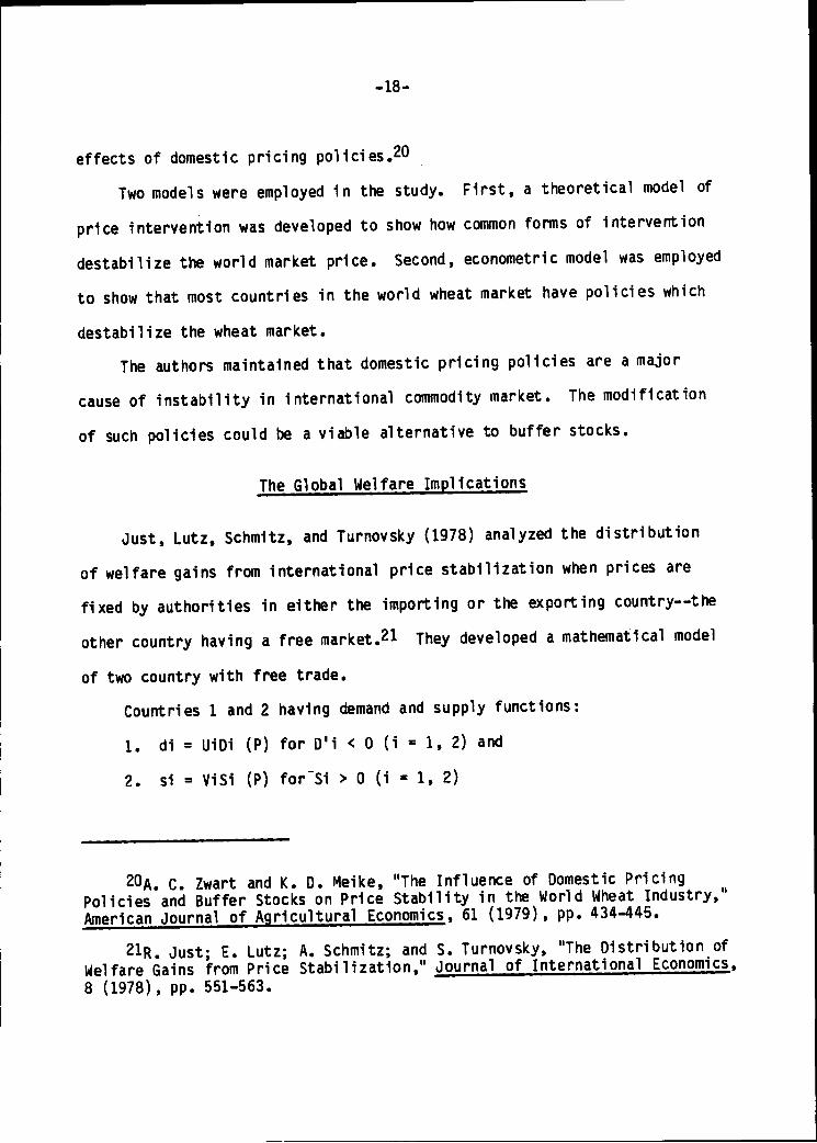
effects of domestic pricing policies.20
Two models were employed in the study. First, a theoretical model of
price intervention was developed to show how common forms of intervention
destabilize the world market price. Second, econometric model was employed
to show that most countries in the world wheat market have policies which
destabilize the wheat market.
The authors maintained that domestic pricing policies are a major
cause of instability in international commodity market. The modification
of such policies could be a viable alternative to buffer stocks.
The Global Welfare Implications
Just, Lutz, Schmitz, and Turnovsky (1978) analyzed the distribution
of welfare gains from international price stabilization when prices are
fixed by authorities in either the importing or the exporting country—the
other country having a free market.21 They developed a mathematical model
of two country with free trade.
Countries 1 and 2 having demand and supply functions:
1. di = UiDi (P) for D'i < 0 (i = 1, 2) and
2. si = ViSi (P) for'Si > 0 (1 - 1, 2)
2°A. C. Zwart and K. D. Meike, "The Influence of Domestic PricingPolicies and Buffer Stocks on Price Stability in the World Wheat Industry,American Journal of Agricultural Economics, 61 (1979), pp. 434-445.
2lR. Just; E. Lutz; A. Schmitz; and S. Turnovsky, "The Distribution ofWelfare Gains from Price Stabilization," Journal of International Economics,
8 (1978), pp. 551-563.
-19-
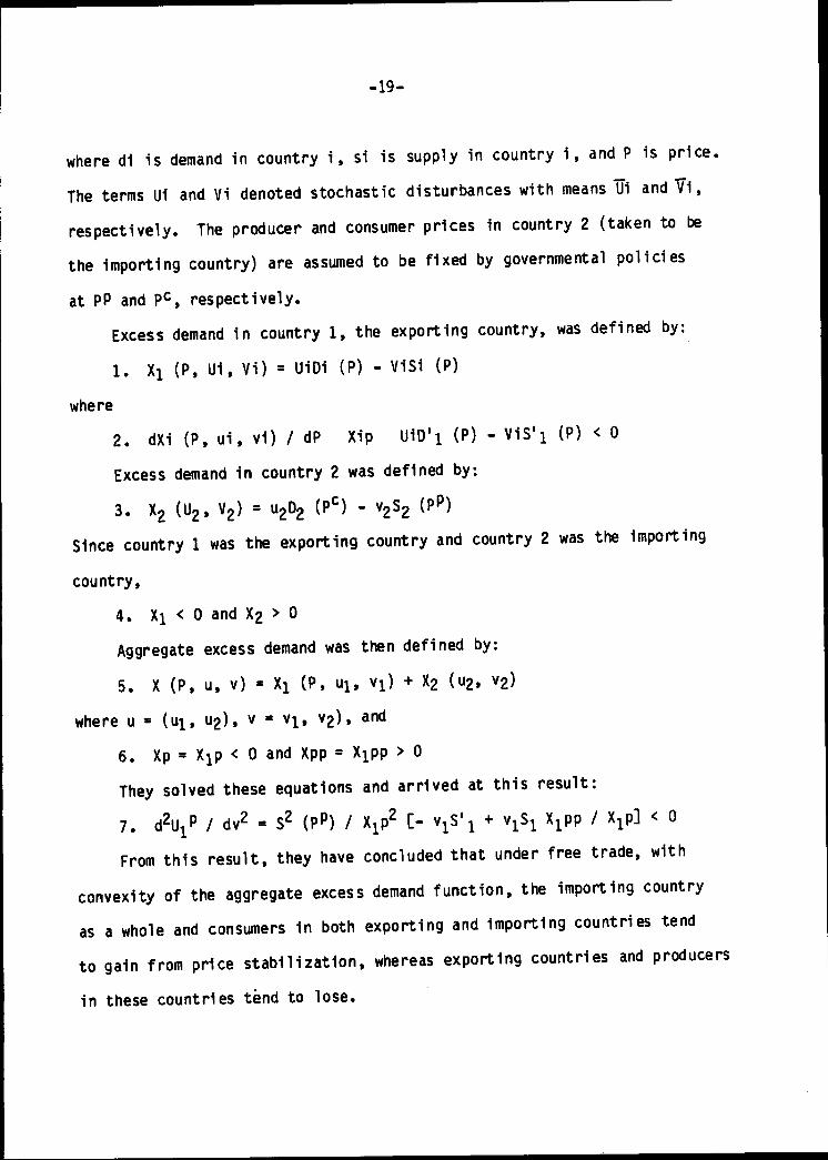
where di is demand in country i, si is supply in country i, and P is price.
The terms Ui and Vi denoted stochastic disturbances with means Hi and Vi,
respectively. The producer and consumer prices in country 2 (taken to be
the importing country) are assumed to be fixed by governmental policies
at PP and Pc, respectively.
Excess demand in country 1, the exporting country, was defined by:
1. XX (P, Ui, Vi) = UiDi (P) - ViSi (P)
where
2. dXi (P, ui, vi) / dP Xip UiD'i (P) - ViS'i (P) < 0
Excess demand in country 2 was defined by:
3. X2 (U2, V2) = u2D2 (Pc) - v2S2 (PP)
Since country 1 was the exporting country and country 2 was the importing
country,
4. Xi < 0 and X2 > 0
Aggregate excess demand was then defined by:
5. X (P, u, v) = Xi (P, ult vj) + X2 (u2, v2)
where u = (ui, u2), v = vlf v2), and
6. Xp ■ Xxp < 0 and Xpp - Xxpp > 0
They solved these equations and arrived at this result:
7. dV / dv2 = S2 (PP) / XlP2 [- v^'i + VlSx XlPP / XlP] < 0
From this result, they have concluded that under free trade, with
convexity of the aggregate excess demand function, the importing country
as a whole and consumers in both exporting and importing countries tend
to gain from price stabilization, whereas exporting countries and producers
in these countries tend to lose.
-20-
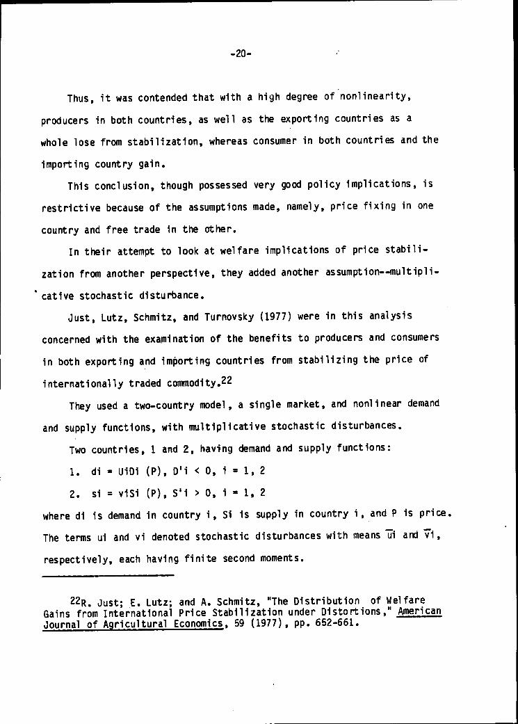
Thus, it was contended that with a high degree of nonlinearity,
producers in both countries, as well as the exporting countries as a
whole lose from stabilization, whereas consumer in both countries and the
importing country gain.
This conclusion, though possessed very good policy implications, is
restrictive because of the assumptions made, namely, price fixing in one
country and free trade in the other.
In their attempt to look at welfare implications of price stabili
zation from another perspective, they added another assumption—multipli
cative stochastic disturbance.
Just, Lutz, Schmitz, and Turnovsky (1977) were in this analysis
concerned with the examination of the benefits to producers and consumers
in both exporting and importing countries from stabilizing the price of
internationally traded commodity.22
They used a two-country model, a single market, and nonlinear demand
and supply functions, with multiplicative stochastic disturbances.
Two countries, 1 and 2, having demand and supply functions:
1. di * UiDi (P), D'i < 0, i = 1, 2
2. si = viSi (P), S'i > 0, i = 1, 2
where di is demand in country i, Si is supply in country i, and P is price.
The terms ui and vi denoted stochastic disturbances with means Hi and vi,
respectively, each having finite second moments.
22R. Just; E. Lutz; and A. Schmitz, "The Distribution of WelfareGains from International Price Stabilization under Distortions," AmericanJournal of Agricultural Economics, 59 (1977), pp. 652-661.
-21-
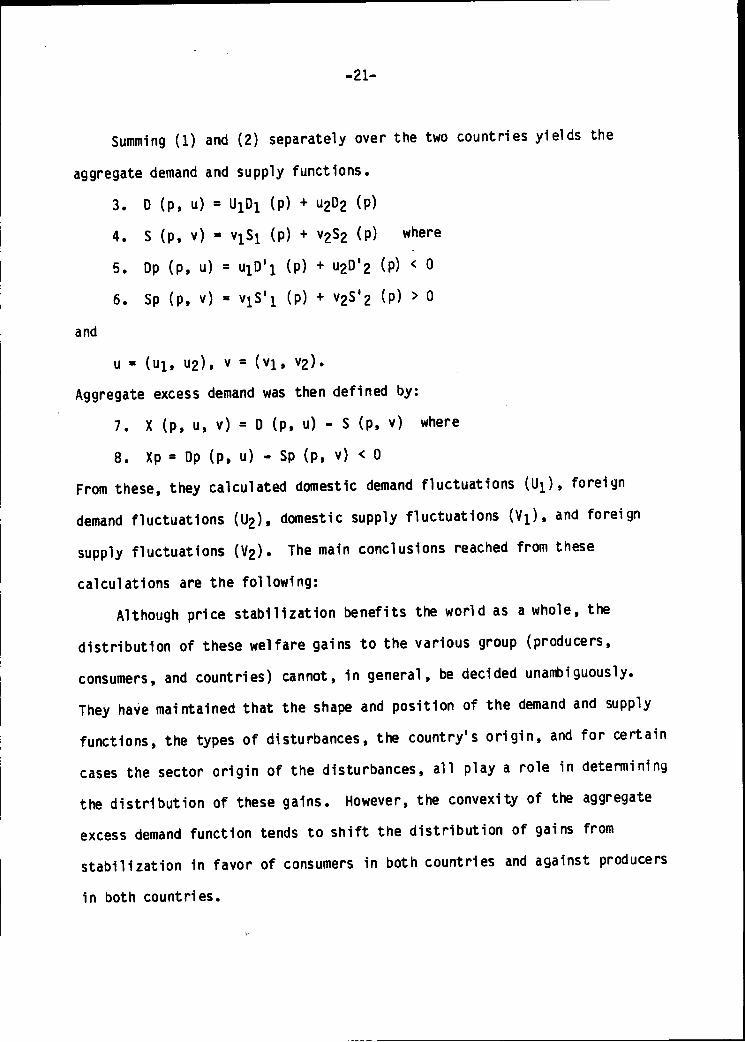
Summing (1) and (2) separately over the two countries yields the
aggregate demand and supply functions.
3. D (p, u) = UiDi (p) + u2D2 (p)
4. S (p, v) = v^i (p) + v2S2 (p) where
5. Dp (p, u) = UiD'i (p) + u2D'2 (p) < 0
6. Sp (p, v) = ViS'x (p) + v2S'2 (p) > 0
and
u ■ (ui, u2), v = (vi, v2).
Aggregate excess demand was then defined by:
7. X (p, u, v) = D (p, u) - S (p, v) where
8. Xp = Dp (p, u) - Sp (p, v) < 0
From these, they calculated domestic demand fluctuations (u"i), foreign
demand fluctuations (U2), domestic supply fluctuations (V^, and foreign
supply fluctuations (V2). The main conclusions reached from these
calculations are the following:
Although price stabilization benefits the world as a whole, the
distribution of these welfare gains to the various group (producers,
consumers, and countries) cannot, in general, be decided unambiguously.
They have maintained that the shape and position of the demand and supply
functions, the types of disturbances, the country's origin, and for certain
cases the sector origin of the disturbances, all play a role in determining
the distribution of these gains. However, the convexity of the aggregate
excess demand function tends to shift the distribution of gains from
stabilization in favor of consumers in both countries and against producers
in both countries.
-22-
Massell (1970) evaluating the same question—welfare implications of
international price stabilization—restricted his analysis to a single
market.23 He presented a diagrammatic and an analytical frameworks that
involved maximization of a producer's welfare function.
The welfare function contained as arguments the mean and variance
of income and was assumed to be increasing in the former argument and
decreasing in the latter. From the graphs, the author showed that producers
are able to compensate consumers so as to leave both groups better off from
price stability.
He contended that actual compensation was needed before it can be
concluded that price stability is preferred to price instability.
However, no attempt was made in the analysis to determine whether or
not price stabilization is socially desirable for individual trading
nations in the absence of either domestic or international compensation.
Sandrum (1975), considering welfare gains and price stabilization,
rejected the main point Massell made in his article.24 Massell's analysis
has the advantage that the expressions measuring the welfare gains from
stabilization can be calculated explicitly. Sandrum contended that much
relevant empirical work finds non-linear relationships, such as log-linear
functions, to be superior, in which case the Massell's results are
inapplicable.
23B. F. Massell, "Some Welfare Implications of International PriceStabilization," Journal of Political Economy, LXXVII (1970), pp. 404-417
r. M. Sandrum, "Welfare Gains from Price Stabilization," Canadian
Journal of Economics, 11 (1976), pp. 133-147.
-23-
Sandrum's analysis was also confined to a single market, but with
the assumption of multiplicative disturbances. He used the production
functions and utility functions which underly the market supply and demand
function, and evaluated the behavior of the supply side and the demand
side independently and mathematically.
He stressed that the distribution of welfare gains from introducing
a price stabilization scheme in a situation where the random disturbances
are multiplicative, differ from those obtained by previous authors. The
most important general difference is that the desirability of price
stabilization for either producers or consumers does not depend upon the
source of the price instability, but rather, upon the shapes of the deter
ministic components of the demand and supply curves. He maintained that if
one group benefits from having price stabilized, it will do so whether the
random price arises from stochastic disturbances in demand or in supply.
It was the author's view that producers gain from having either the
demand or supply disturbances stabilized if demand is elastic and supply
inelastic, while they lose in the reverse situation. Similarly, consumers
tend to gain if supply is elastic and demand is inelastic and be worse off
otherwise.
In order to evaluate the issue of welfare implications of grain price
stabilization, using a specific product, and from the point of view of an
exporting country, Konandreas (1978) restricted his analysis to the United
States; since the United States is an exporter of wheat.25
25p. l. Konandreas, "Implications of Grain Price Stabilization,"Canadian Journal of Economics, 32 (1978), pp. 501-517.
-24-
The model specified a United States domestic demand relationship for
food and feed use; a stock relationship and a foreign demand sector; these
were estimated by Ordinary and Two-Stage Least Squares methods.
The empirical study demonstrates that although the United States'
producers and consumers taken together benefit from policies which would
stabilize feed grain prices, this is not likely the case for wheat.
Finally, the central issue—who gains or who loses—is brought to bear
in this analysis.
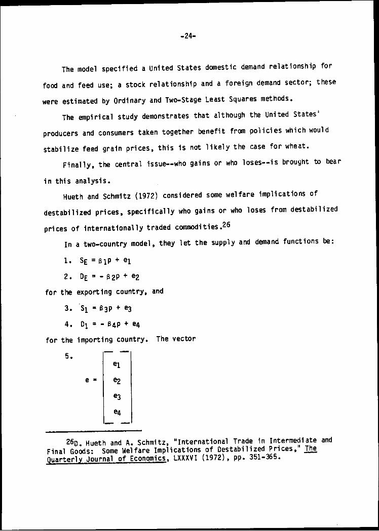
Hueth and Schmitz (1972) considered some welfare implications of
destabilized prices, specifically who gains or who loses from destabilized
prices of internationally traded commodities.26
In a two-country model, they let the supply and demand functions be:
1. Se a 3iP + ei
2. DE = - 32P + e2
for the exporting country, and
3. Si = B3P + e3
4. Oi - - B4P + e4
for the importing country. The vector
5.
e = e2
e4
26q. Hueth and A. Schmitz, "International Trade in Intermediate andFinal Goods: Some Welfare Implications of Destabilized Prices, TheQuarterly Journal of Economics, LXXXVI (1972), pp. 351-365.
-25-
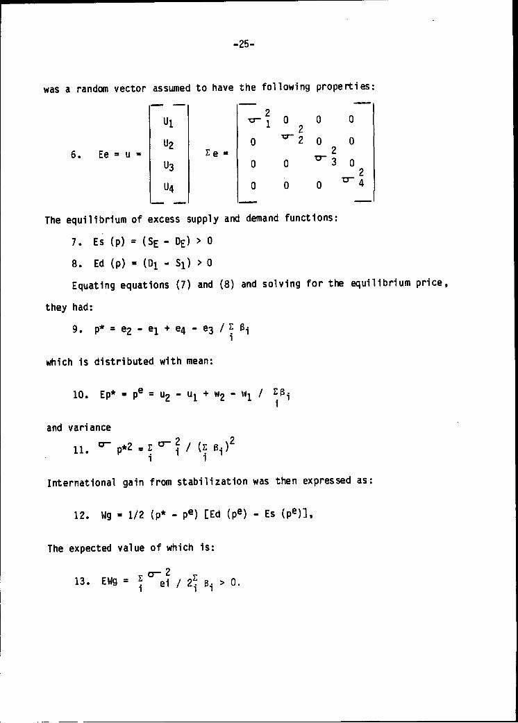
was a random vector assumed to have the following properties:
6. Ee = u =
"1
U2
U3
U4
1
10 ^
0 0
0 0 0
0 02
^3 02
4
The equilibrium of excess supply and demand functions:
7. Es (p) = (SE - DE) > 0
8. Ed (p) = (Di - Si) > 0
Equating equations (7) and (8) and solving for the equilibrium price,
they had:
9. p* " el + e4 " e3 / ? ei
which is distributed with mean:
10. Ep* = pe - u2 - uj + w2 - wx / 2S.
and variance
u. °-p*2aE°-2/ (j Bi)2
International gain from stabilization was then expressed as
12. Wg = 1/2 (p* - pe) [Ed (pe) - Es (pe)],
The expected value of which is:
13. EWg = * ei 0.

-26-
From these results, they have concluded that when one uses the
expected value of the change in producer and consumer surplus as a measure
of gain, price stabilization brought about a buffer stock, results in a
net gain to world consumers and producers. But actual compensation is
needed to obtain this result, and it must be at an international level.
It was also shown that in the absence of compensation, producers or
consumers in all countries do not gain or lose from price stability.
Summary
This literature review brings to focus the following pointsf
1. The major wheat exporting countries determine wheat prices
because of their capacity to hold stock;
2. Protectionism has global effects including fluctuation of prices
at the world market; and
3. The welfare implications show that whether or not an individual
country benefits from price stability depends on th source of the
instability; when the source of instability originates in only
one of the two countries considered, that country will always
prefer stabilized prices if domestic compensation is paid; price
instability is preferable for the country that does not contribute
to instability. If both countries contributes to price instability,
the results, with respect to which country gains from price
stabilization, are inconclusive. Finally, regardless of the source
or extent of the instability when international compensation is
paid, price stabilization is a desirable policy for both world
consumers and producers.

CHAPTER III
THEORETICAL FRAMEWORK
Three models are employed in the analysis of this paper. First,
standard partial equilibrium comparative static analysis in the Marshallian
economic surplus framework27--welfare theory—is used for the estimation
of the following.
Net social loss in production
NSLp = 1/2 (Qw - Q) (Pw - Pp) = 1/2 tp2nsV (1)
Net social loss in consumption
NSLc = 1/2 (Cw - C) (Pc - Pw) = 1/2 tc2 nd w; (2)
Welfare gain of producers
Gp = Q (pp - Pw) - NSLp; and (3)
Welfare gain of consumers
Gc = C (Pw - Pc) - NSLc
The variables are defined as follows:
Qw » Production at world price;
Q a production at domestic price;
Pw = World price;
Pp a Price received by farmers;
Pc = Price faced by domestic consumers;
27j. M. Currie; J. A. Martin; and A. Schmitz, "The Concept of EconomicsSurplus and Its Use in Economic Analysis," Economic Journal, 81 (1971),p. 743.
-27-
-28-
V ■ Value of production at Pp;
W - Value of consumption at Pc;
Cw ■ Consumption at world price;
C = Consumption at domestic price;
ns = Elasticity of supply;
nd = Elasticity of demand;
tc = Proportion of tariff at the consumer level; and
tp ■ Proportion of tariff at the producer level.
The proportion of tariff at the consumer level is defined as the
difference between the price faced by domestic consumers and the world
price. Also, the proportion of tariff at the producer level is defined as
the difference between the price at the producer level and the world price.
The following assumptions are made in this paper:
1) The United States is an exporter of wheat;
2) The demand function is linear and negatively sloped;
3) The supply function is linear and positively sloped;
4) World price is equilibrium price, and at this price the difference
between quantity supplied and demanded is zero; and
5) The quantity of wheat not exported is consumed domestically, i.e.,
the difference between the quantity produced, and the quantity
exported is domestically consumed.
Second, a Marshallian demand function28~theory of consumer behavior-
is employed through the use of Ordinary Least Squares Techniques to estimate
28J. H. Henderson and R. E. Quandt, Microeconomic Theory: A Mathematical Approach, Third Edition (New York"- McGraw-Hill Book, Inc., 1980).
-29-
the parameters in the aforementioned welfare theory.
The demand function gives the quantity of a commodity that a consumer
will buy as a function of the commodity prices and the consumer's income.29
Mathematically, this model can be represented as follows:
Qd = f(Plt P2, Y°) (5)
This relationship satisfies the general assumption that demand
functions are negatively sloped—the lower the price, the greater the
quantity demanded. However, this study assumes a multiplicative relation
ship of the following form:
Qdw ■ aoPalYa2 (6)
which upon logarithmic transformation yields:
Qdw = logao + ajlogP + a2logY + U (7)
Qdw = Quantity of wheat demanded;
ao = The constant which represents the intercept coefficient;
ai - The price coefficient defined to satisfy the price elasticity
interpretation;
a2 - The positive income coefficient, also defined to satisfy the
income elasticity interpretation; and
U » The error term.
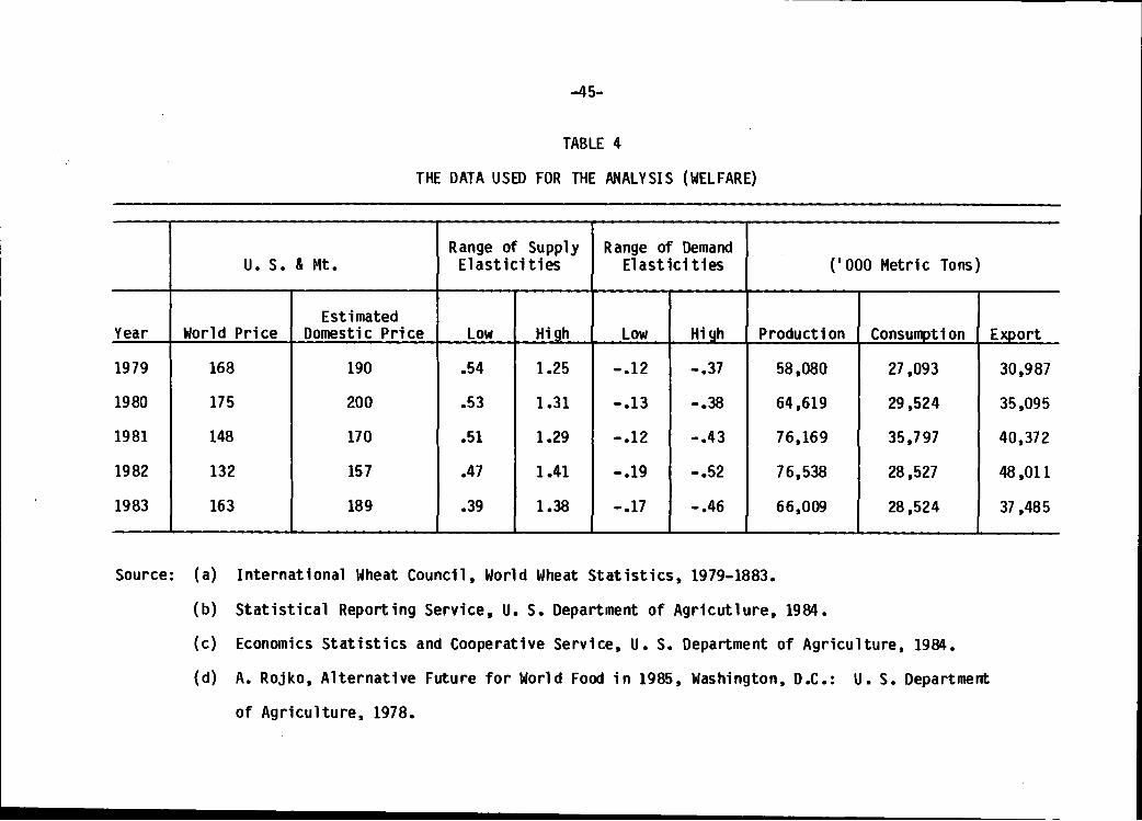
Third, it is found that the wheat prices in the United States are
greater than the equilibrium prices—world prices (Table 4). In order to
show the effects of equilibrium price on the quantity of wheat in this
29j. H. Henderson and R. E. Quandt, Microeconomic Theory: A Mathematical Approach, Third Edition (New York: McGraw-Hill Book, Inc., 1980).
-30-
country, partial equilibrium market model,30 i.e., a linear model of price
determination in an isolated market is employed.
The mathematical representations with defined parameters are as
follows:
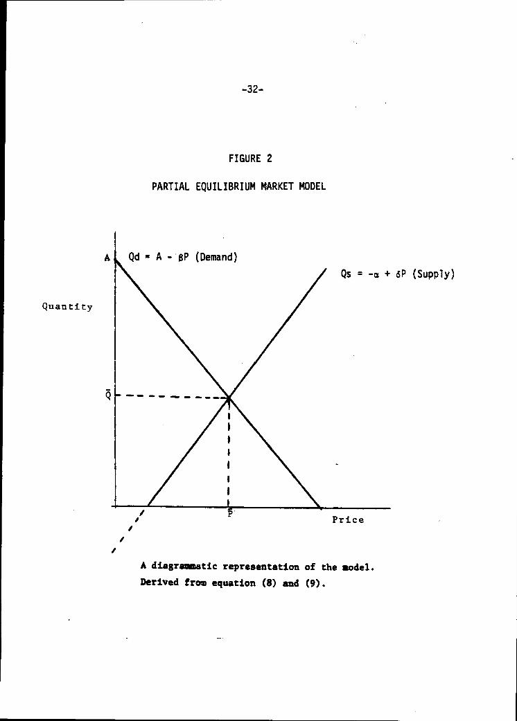
Qd - A - BP: The demand function (8)
Qs = -a + 6 P: The supply function (9)
A, 3 , a , and 6 are exogenous parameters defined to be greater than
zero.
Qd ■ Qs: The equilibrium condition.
(A - BP)-(-o + 6P): Setting Qd = Qs (10)
Thus, the equilibrium price:
•p =(A +a)/(g + 6) . p > 0 (11)
To obtain the equilibrium quantity, the equilibrium pice is substituted
into either the supply or demand equation.
Q" = A - B A+a /(B +6)=(A6- Ba)/(B + 6) * A6 > 6a (Ha)
The purpose of this exercise is to show how the equilibrium value of
an endogenous variable will change as a result of a change of any of the
exogenous parameters. This is done to depict the situation of wheat market
from the point of view of this country, and within the confines of
comparative-static analysis.
It was determined that the equilibrium price
"P =(A + a)/(B+ 6) , and (12)
30A. C. Chiang, Fundamental Methods of Mathematical Economics, SecondEdition (New York: McGraw-Hill Book, Inc., 1974).
-31-
since the emphasis is on the effect on quantity as a result of an increase
in price, the analysis is restricted to the equilibrium price result.
dT / 9A = 1 / 6 +• 6 : (13)
g-p / 3g - -(A + a) / (3 +6)2 (14)
3P" / 3o - 1 / B +■ « : <15)
3"p / 96= -(A + a) / (3 +- 6)2 (16)
Because A, 3, a, and 6 > 0, then
3P / 3A = 3"P / 3a > 0 and 3P" / 33 = 3P" / 3 6 < 0.
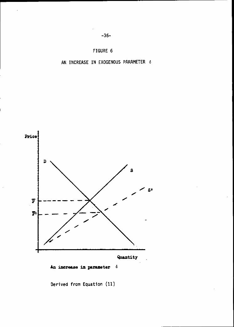
Diagrammatic representations (Figures 3, 4, 5 and 6) are provided to
delineate the effect on price, and consequently on quantity as a result
of a change in any of the exogenous parameters.
As evident on the graphs (Figures 3 and 5), increase in parameters A
and a will raise the level of prices. However, the increase in prices as
a result of a change in parameter a will consequently reduce the quantity
levels. From the point of view of this study, therefore, exogenous
parameter a then becomes income-support deficiency payment programs, "set-
aside" schemes, and subsidies; since these are the programs used by
authorities to distort the prices of agricultural commodities. These
results will remain vaild, regardless of specific values that the parameters
A, 3, a , and 6 take, as long as they satisfy the sign restriction.
This author proposes that the effect on quantity as a result of an
increase in parameters a will hold true in the wheat market of this country
because of the following:
-32-
FIGURE 2
PARTIAL EQUILIBRIUM MARKET MODEL
Qd ■ A - 8P (Demand)
Quantity
Qs = -o + 5P (Supply)
Price
A diagrammatic representation of the model.
Derived from equation (8) and (9).
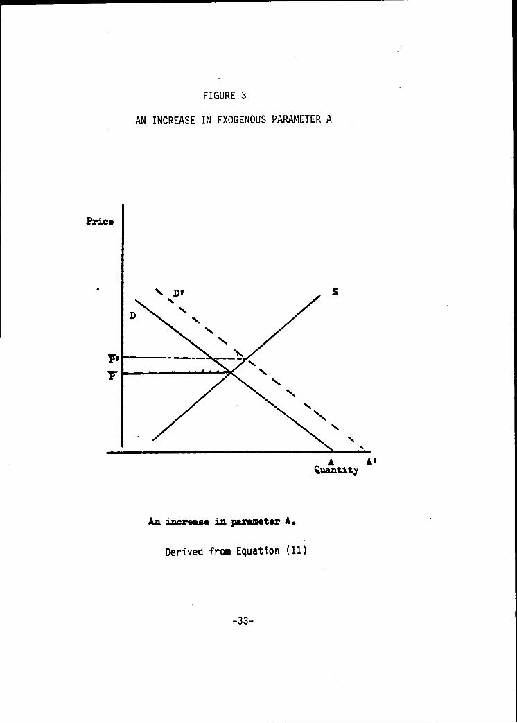
FIGURE 3
AN INCREASE IN EXOGENOUS PARAMETER A
Price
A A*Quantity
An increase in parameter A.
Derived from Equation (11)
-33-

FIGURE 4
AN INCREASE IN EXOGENOUS PARAMETER B
Price
Quantity
increase ia parameter 0
Derived from Equation (11)
-34-
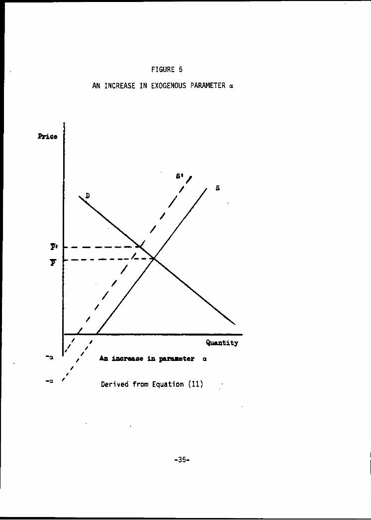
FIGURE 5
AN INCREASE IN EXOGENOUS PARAMETER a
Price
Quantity
-a
An increase in parameter a
Derived from Equation (11)
-35-
-36-
FIGURE 6
AN INCREASE IN EXOGENOUS PARAMETER <5
Price
S
7*
s«
Quantity
An increase in parameter
Derived from Equation (11)
-37-
1) Despite the fact that the United Stastes is a major wheat
exporter, it does not have the resources to monopolize the
world market price. This is solely because of the influence
exerted at the market by other major wheat exporters—Canada
and Australia.
2) For any individual country to have a considerable influence on
the world market, it must have a price that is commensurable
with the world price.
CHAPTER IV
SUMMARY OF REGRESSIONS
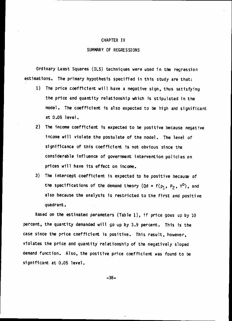
Ordinary Least Squares (OLS) techniques were used in the regression
estimations. The primary hypothesis specified in this study are that:
1) The price coefficient will have a negative sign, thus satisfying
the price and quantity relationship which is stipulated in the
model. The coefficient is also expected to be high and significant
at 0.05 level.
2) The income coefficient is expected to be positive because negative
income will violate the postulate of the model. The level of
significance of this coefficient is not obvious since the
considerable influence of government intervention policies on
prices will have its effect on income.
3) The intercept coefficient is expected to be positive because of
the specifications of the demand theory (Qd = f(pj, P2, Y°), and
also because the analysis is restricted to the first and positive
quadrant.
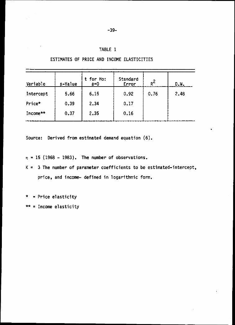
Based on the estimated parameters (Table 1), if price goes up by 10
percent, the quantity demanded will go up by 3.9 percent. This is the
case since the price coefficient is positive. This result, however,
violates the price and quantity relationship of the negatively sloped
demand function. Also, the positive price coefficient was found to be
significant at 0.05 level.
-38-
-39-
TABLE 1
ESTIMATES OF PRICE AND INCOME ELASTICITIES
Variable
Intercept
Price*
Income**
8-Value
5.66
0.39
0.37
t for Ho:
0=0
6.15
2.34
2.35
Standard
Error
0.92
0.17
0.16
R2
0.76
D.W.
2.48
Source: Derived from estimated demand equation (6).
n = 15 (1968 - 1983). The number of observations.
K = 3 The number of parameter coefficients to be estimated-intercept,
price, and income- defined in logarithmic form.
* = Price elasticity
** = Income elasticity
-40-
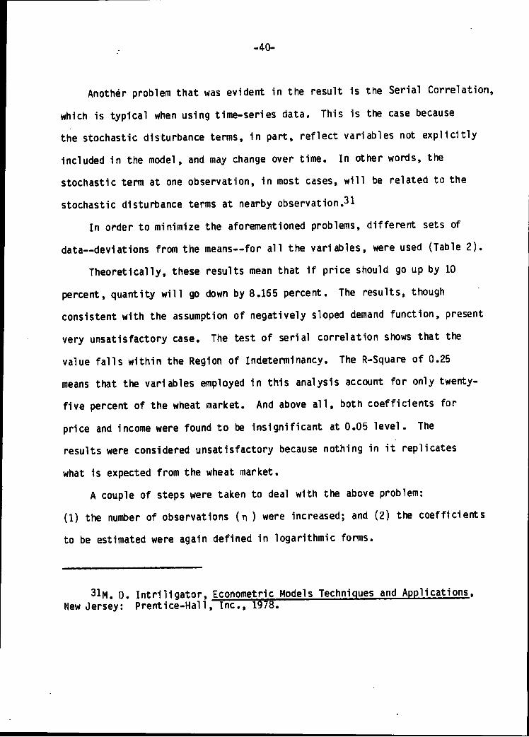
Another problem that was evident in the result is the Serial Correlation,
which is typical when using time-series data. This is the case because
the stochastic disturbance terms, in part, reflect variables not explicitly
included in the model, and may change over time. In other words, the
stochastic term at one observation, in most cases, will be related to the
stochastic disturbance terms at nearby observation.31
In order to minimize the aforementioned problems, different sets of
data—deviations from the means—for all the variables, were used (Table 2).
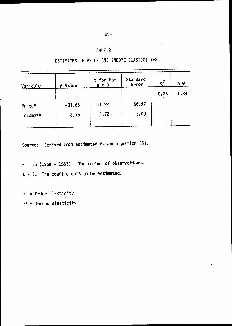
Theoretically, these results mean that if price should go up by 10
percent, quantity will go down by 8.165 percent. The results, though
consistent with the assumption of negatively sloped demand function, present
very unsatisfactory case. The test of serial correlation shows that the
value falls within the Region of Indeterminancy. The R-Square of 0.25
means that the variables employed in this analysis account for only twenty-
five percent of the wheat market. And above all, both coefficients for
price and income were found to be insignificant at 0.05 level. The
results were considered unsatisfactory because nothing in it replicates
what is expected from the wheat market.
A couple of steps were taken to deal with the above problem:
(1) the number of observations (n ) were increased; and (2) the coefficients
to be estimated were again defined in logarithmic forms.
31M. D. Intriiigator. Econometric Models Techniques and Applications,
New Jersey: Prentice-Hall, Inc., 1978.
-41-
TABLE 2
ESTIMATES OF PRICE AND INCOME ELASTICITIES
Variable 8 Value
t for Ho:
6 = 0
Standard
Error D.W
Price*
Income**
-81.65
8.75
-1.22
1.72
66.97
5.09
0.25 1.34
Source: Derived from estimated demand equation (6),
t) = 15 (1968 - 1983). The number of observations.
K = 3. The coefficients to be estimated.
* = Price elasticity
** = Income elasticity
-42-
TABLE 3
ESTIMATES OF PRICE AND INCOME ELASTICITIES
Variable
Intercept
Price*
Income**
6-Value
8.11
-.79
0.22
t
3
4
-2
1
for Ho:
= 0
.23
.00
.65
Standard
Error
1.92
0.39
0.21
R2
0.88
D
2
.W.
.12
Source: Derived from estimated demand equation (6).
n = 25. The number of observations (1958 - 1983).
K = 3. The parameter coefficient to be estimated; defined in
logarithmic form.
* = Price elasticity
** = Income elasticity
-43-
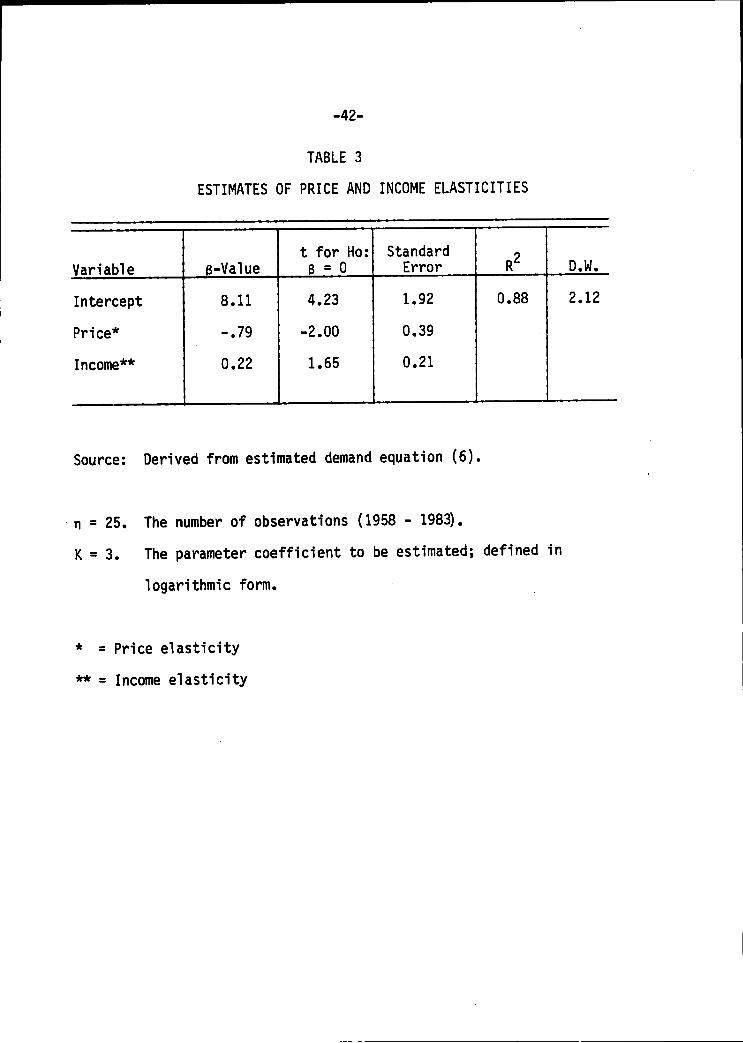
The estimated parameters (Table 3) show that if price should go up
by ten percent, the quantity demanded will go down by seventy-nine percent.
The coefficient for price, as shown by the results is negative. This
is as expected, and is consistant with the postulate of the model, namely,
negatively sloped demand curve—the lower the price, the greater the
quantity demanded. Also, the coefficient is found to be significant at
.05 level.
Although this value (-0.79) is greater than the elasticities used
in this study, it is deemed representatives of what is expected from the
wheat market, and consistent with the results of earlier studies in this
area.32
The income coefficent is positive as expected, but insignificant at
.05 level. This result brings to the open the central premise of this
study—protectionism. It is not certain if the dominance of government
intervention policies, as characterized by "set-aside" schemes, "deficiency
payment programs," and subsidies, have rendered income of no major effect
in the wheat market. However, the coefficient is found to be significant
at 0.1 level.
The R-square value is 0.88. This means that eighy-eight percent of
the wheat market is explained by the variables employed in this study.
It should also be stressed that this result is representative of earlier
32P. A. Carter, "Quotas and Pricing of Agricultural Commodities,"Canadian Journal of Economics, 13 (1976), p. 552.
-44-
studies on price distortions by authorities.33
The Oubin-Watson statistic shows that there is no problem of serial
correlation between the dependent and explanatory variables. These results
compare favorably with earlier studies on government intervention pricing
policies. Specifically, Bale and Lutz have contended that the quantitative
results of government intervention of agricultural products on prices
depended on the slopes of the supply and demand functions as well as on
the size of the demand and supply disturbances.34
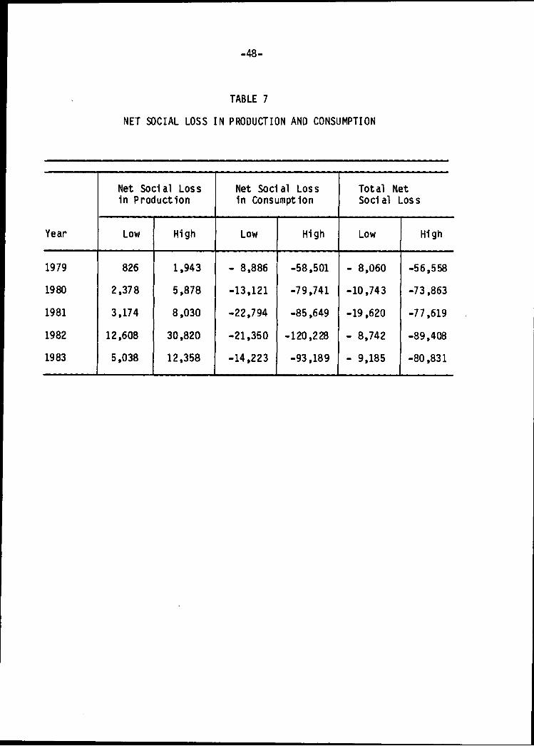
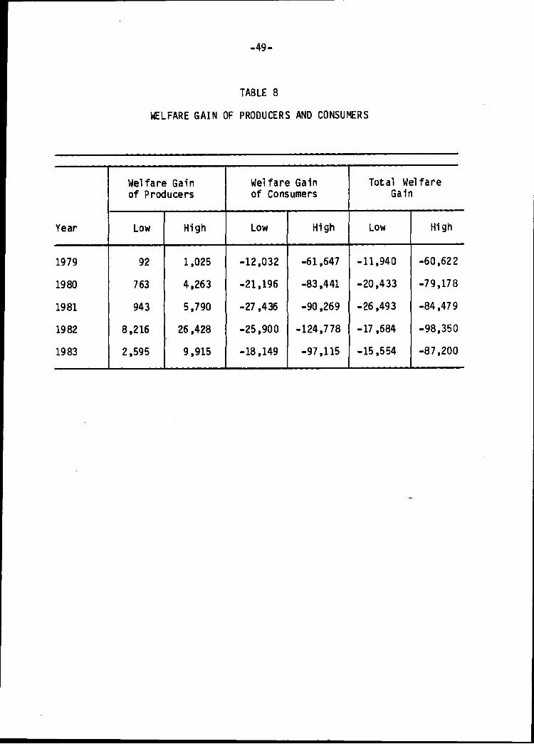
Welfare Measurement
In order to show the extent of the effects of protectionism on the
welfare of consumers, we reestimate the net social loss in consumption
and welfare gain of consumers, using the elasticity obtained in this study
(Table 3). As shown in Tables 7 and 8, the welfare implications were
underestimated by Rojko (Table 4). However, there is no contradiction
between the results of the two estimations.
33p. L. Konandreas, "Welfare Implication of Grain Price Stabilization,"Journal of Economics, 12 (1975), p. 511.
34m. D. Bale and E. Lutz, "The Effects of Trade Intervention onInternational Price Instability," American Journal of Agricultural
Economics, 61 (1979), p. 515.
-45-
TABLE 4
THE DATA USED FOR THE ANALYSIS (WELFARE)
Year
1979
1980
1981
1982
1983
U. S.
World Price
168
175
148
132
163
& Mt.
Estimated
Domestic Price
190
200
170
157
189
Range of Supply
Elasticities
Low
.54
.53
.51
.47
.39
High
1.25
1.31
1.29
1.41
1.38
Range of Demand
Elasticities
Low
-.12
-.13
-.12
-.19
-.17
High
-.37
-.38
-.43
-.52
-.46
('000 Metric Tons)
Production
58,080
64,619
76,169
76,538
66,009
Consumption
27,093
29,524
35,797
28,527
28,524
Export
30,987
35,095
40,372
48,011
37 ,485
Source: (a) International Wheat Council, World Wheat Statistics, 1979-1883.
(b) Statistical Reporting Service, U. S. Department of Agricutlure, 1984.
(c) Economics Statistics and Cooperative Service, U. S. Department of Agriculture, 1984.
(d) A. Rojko, Alternative Future for World Food in 1985, Washington, D.C.: U. S. Department
of Agriculture, 1978.
-46-
TABLE 5
NET SOCIAL LOSS IN PRODUCTION AND CONSUMPTION
Year
1979
1980
1981
1982
1983
2
3
12
5
Net Social Loss
in Production
Low
826
,378
,174
,608
,038
High
1,943
'5,878
8,030
30,820
12,358
i ■
Net Social Loss
in Consumption
n 'nnn n <
Low
- 8,886
-13,121
-22,794
-21,350
-14,223
; Dollars}-
High
-27,399
-38,356
-74,081
-62,525
-42,671
Total
Soci al
Low
- 8,060
-10,743
- 8,742
- 8,742
- 9,185
Net
Loss
High
-25,456
-32,478
-66,051
-31,705
-30,313
-47-
TABLE 6
WELFARE GAIN OF PRODUCERS AND CONSUMERS
Year
1979
1980
1981
1982
1983
Welfare Gain
of Producers
Low
92
763
943
8,216
2,595
High
1,025
4,263
5,790
26,428
9,915
Welfare Gain
of Consumers
n 'nnn u c
Low
-12,032
-21,196
-27,436
-25,900
-18,149
: nollars}-
High
-30,545
-46,431
-78,723
-67,075
-46,597
Total Welfare
Gain
Low
-11,940
-20,433
-26,493
-17,684
-15,554
High
-29,520
-42,168
-72,933
-40,647
-36,682
-48-
TABLE 7
NET SOCIAL LOSS IN PRODUCTION AND CONSUMPTION
Year
1979
1980
1981
1982
1983
Net Social Loss
in Production
Low
826
2,378
3,174
12,608
5,038
High
1,943
5,878
8,030
30,820
12,358
Net Social Loss
in Consumption
Low
- 8,886
-13,121
-22,794
-21,350
-14,223
High
-58,501
-79,741
-85,649
-120,228
-93,189
Total Net
Social Loss
Low
- 8,060
-10,743
-19,620
- 8,742
- 9,185
High
-56,558
-73,863
-77,619
-89,408
-80,831
-49-
TABLE 8
WELFARE GAIN OF PRODUCERS AND CONSUMERS
Year
1979
1980
1981
1982
1983
Welfare Gain
of Producers
Low
92
763
943
8,216
2,595
High
1,025
4,263
5,790
26,428
9,915
Welfare Gain
of Consumers
Low
-12,032
-21,196
-27,436
-25,900
-18,149
High
-61,647
-83,441
-90,269
-124,778
-97,115
Total Welfare
Gain
Low
-11,940
-20,433
-26,493
-17,684
-15,554
High
-60,622
-79,178
-84,479
-98,350
-87,200
CHAPTER V
SUMMARY
This study was concerned with a quantification of the effects of
government intervention in the pricing of wheat in the United States.
Standard partial equilibrium comparative static analysis in the Marshallian
economic surplus framework was used in the calculations of net social loss
in production and consumption, and welfare gain of producers and consumers.
The method of Ordinary Least Squares (OLS) was employed to estimate the
parameter coefficients in the aforementioned model.
In the analysis, world wheat price was assumed to be the equilibrium
price, and "partial market equilibrium"~a linar model--was used to
elaborate on the effect on quantity of a price greater than the equilibrium
price.
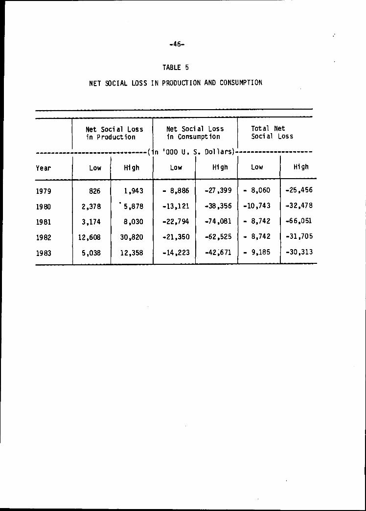
It was determined in this study that government intervention in the
pricing of wheat has a negative rate of protection on the domestic
consumption of wheat; i.e., the quantity of wheat consumed in this country
is substantially less than the quantity it would have been in the absence
of price distortions (Table 5).
Results
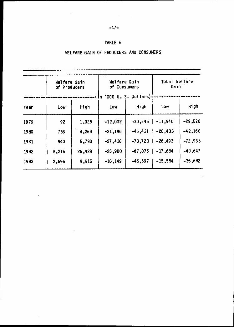
1) The intervention policies have positive rate of protection on
production (Table 6). As a result, the levels of production under
protectionism are higher than they would be in the absence of price
distortions.
-50-
-51-
2) The importing country's imports and domestic consumption of wheat will
both increase; a direct result of the pricing policies of the exporting
country.
3) The total net social loss and net welfare gain were both found to be
negative in this study. The results bring home the central issue in
this analysis, namely, that the problems created by protectionism far
exceed the benefits to the producers.
4) The net social loss in production turned out to be positive confirming
the main postulate of this study—a price greater than the equilibrium
price will reduce the quantity demanded. However, this result is a
constrast to the one stated earlier that production levels under
protectionism are higher than they would otherwise be.
The following reasons account for this discrepancy:
1) The wheat in the United States is a "special market." It is a market
where the interaction of forces of demand and supply are almost
absent. The market, to a greater extent, is characterized by the
dictates of government authorities.
2) The stockholding capacity of this country is another factor that
plays a very significant role in the wheat market. What is indubit
able in this analysis is that yearly demand has little or nothing to
do with yearly production. This is the justification for the effects
of the embargo which were neither seen on production nor on prices.
-52-
Conciusion and Policy Consideration
The key point evident in this study is that the loss to consumers as
a result of protectionism far exceed the benefits that accrue to the
producers. As a result, government authorities are spending enormous
amount of money to keep this program going. Bale and Lutz, analyzing
this problem, have said "In recent years, deficiency payment in the
United States have ranged from $800 million to $4 bill ion,...and one of
the causes of misallocated resources use."35
The considerable influence of government pricing policies, as mani
fested in "set-aside" schemes, deficiency payment programs, and subsidies
have bearings in the determination of the quantity demanded in the wheat
market. It is not certain if this influence is responsible for the
insignificance of income at 0.05 level.
Price was found to be the variable that was playing the dominant
role in the wheat market, thus confirming the following:
1) The government authorities of this country are able to prevent foreign
competition because of the substantial influence they have over price.
2) This influence on price is enhanced by hugh inventory—capacity to
hold stock—consequently enabling the retention of this country's
market share.
35M. D. Bale and E. Lutz, "Agricultural Protectionism in IndustrializedNations and Its Global Effects: A Survey of Issues," World Bank Staff
Working Paper, No. 248.
-53-
3) The major wheat exporters—Canada, the United States, and Australia
—as individual countries, do not have the resources to monopolize
the world market price.
4) For any individual country to have a considerable influence on the
world market, it must have a price that is commersurable with world
price.
It is always gratifying to be among the people who are doing their
best to provide the necessary information to help today's world into a
better tomorrow. This endeavor is considered expedient in view of the
quest for excellence which has become an obsession in today's world.
More than before, reliable information is needed in the fields of employ
ment, exports, imports, interest rate, inflation, investment, and a
variety of other issues for prudent legislation formulations and efficient
management. This paper, in all its facets and ramifications, is designed
to be of use, hopefully, in this area.
Suggested Areas for Future Studies
1) There are varied opinions about the shape of the supply and demand
functions of agricultural products. Economists doing studies in this
area have treated these functions on the basis of assumptions—linear
or nonlinear. Since the effectiveness of protectionism depends on
the slopes and elasticities of these functions, determining which of
the two is true will be a useful guide to future studies for the
farm sector.
-54-
2) The estimation of a linear relationship when the actual relationship
is nonlinear is a problem when using Ordinary Least Squares (OLS)
technique, particularly when testing for Serial Correlation (Dubin-
Watson). Like the case of the supply and demand functions, the
stochastic disturbance term has been left to assumptions--additive
or multiplicative—in studies relating to agricultural products.
This author considers this phenomenon a dangerous tendency, since
it is the value of Dubin-Watson that explains the "correlation"
between the dependent and explanatory variables.
Assuming that the nonlinear relationship is estimated by a linear
one, and the stochastic disturbance term is assumed to be additive, the
positive and negative errors would tend to "bunch" together.36 If, on
the other hand, the disturbance term is assumed to be multiplicative,
the results will be very different in a larger magnitude. Thus, deter
mining which of the two is the case will be valuable in many respects.
36M. D. Intriligator, Econometric Models, Techniques and Applications(New Jersey: Prentice-Hall, Inc., 1978).
BIBLIOGRAPHY
Alaouze, C. M.; Watson, A. S.; and Sturgess, N. H. "Oligopoly Pricing
in the World Wheat Market." American Journal of Agricultural
Economics, 60 (1978), pp. 173.185.
Bale, M. D. and Lutz, E. "Agricultural Protectionism in Industrial
Nations and Its Global Effects: A Survey of Issues." World BankStaff Working Paper. No. 248.
. "Price Distortions in Agricultural and Their Effects:An International Comparison." American Journal of Agricultural
Economics, 63 (1981), p. 21.
. "The Effects of Trade Intervention on InternationalPrice Instability." American Journal of Agricultural Economics, 61(1979), pp. 512-516.
Bhagwati, A. "The Effects of Trade Interventions." The Economic Journal.24 (1974), p. 212.
Carter, C. and Schmitz, A. "Import Tariffs and Price Formation in the
World Wheat Market." American Journal of Agricultural Economics,61 (1979), pp. 517-521.
Carter, P. A. "Quotas and Pricing of Agricultural Commodities." CanadianJournal of Economics. 13 (1976), p. 552.
Chiang, A. C. Fundamental Methods of Mathematical Economics. Second
Edition. New York: McGraw-Hill Book, Inc., 1974.
Currie, J. M.; Martin, J. A.; and Schmitz, A. "The Concept of Economics
Surplus and Its Use in Economic Analysis." Economic Journal. 81(1971), p. 743.
Heien, D. "Price Determination Process for Agricultural Sector Models,"American Journal of Agricultural Economics. 59 (1977), p. 126.
Henderson, J. H. and Quandt, R. E. Microeconomic Theory: A Mathematical
Approach. Third Edition. New "York: McGraw-Hill Book, Inc., 1980.
Hueth, D. and Schmitz. "International Trade in Intermediate and FinalGoods: Some Welfare Implications of Destabilized Prices." The
Quarterly Journal of Economics, LXXXVI (1972), pp. 351-365.
Intriligator, M. D. Econometric Models Techniques and Applications.New Jersey: Prentice-Hall, Inc., 1978.
-55-
-56-
Johnson, D. G. "World Agriculture, Commodity Policy, and Price
Variability." American Journal of Agricultural Economics, 56 (1975),
p. 823.
Johnson, H. G. "The Destabilizing Effect of International Commodity
Agreements on the Prices of Primary Products." The Economic Journal,
3 (1950), p. 626.
Just, R.; Lutz, E.; Schmitz, A.; and Turnovsky, S. "The Distribution of
Welfare Gains from Price Stabilization." Journal of International
Economics, 8 (1978), pp. 551-563.
. "The Distribution of Welfare Gains from Interna-
tional Price Stabilization under Distortions." Journal of Interna
tional Economics, 59 (1977), pp. 652-661.
Konandreas, P. L. "Implications of Grain Price Stabilization." Canadian
Journal of Economics, 12 (1975), p. 511.
_. "Implications of Grain Price Stabilization." Canadian
Journal of Economics, 32 (1978), pp. 501-517.
McCalla, A. F. "A Duopoly Model of World Wheat Pricing." Journal of
Farm Economics, 58 (1966), pp. 711-727.
Massell, B. F. "Some Welfare Implications of International Price
Stabilization." Journal of Political Economy, LXXVII (1970),
pp. 404-417.
Sandrum, R. M. "Welfare Gains from Price Stabilization." CanadianJournal of Economics, 11 (1976), pp. 133-147.
Shei, S. Y. and Thompson, R. L. "The Impact of Trade Restrictions on
Price Stability in the World Wheat Market." American Journal of
Agricultural Economics. 59 (1977), p. 629.
World Wheat Statistics. International Wheat Council, London, 1984.
Zwart, A. C. and Meike, K. D. "The Influence of Domestic Pricing Policies
and Buffer Stocks on Price Stability in the World Wheat Industry."
American Journal of Agricultural Economics, 61 (1979), pp. 434-445.