The Geometry of Resonance Tongues:

A Singularity Theory Approach

Henk W. Broer

Department of Mathematics

University of Groningen

P.O. Box 800

9700 AV Groningen

The Netherlands

Martin Golubitsky

Department of Mathematics

University of Houston

Houston, TX 77204-3476

USA

Gert Vegter

Department of Computing Science

University of Groningen

P.O. Box 800

9700 AV Groningen

The Netherlands

October 28, 2002

Abstract

Resonance tongues and their boundaries are studied for nondegenerate and(certain) degenerate Hopf bifurcations of maps using singularity theory meth-ods of equivariant contact equivalence and universal unfoldings. We recover thestandard theory of tongues (the nondegenerate case) in a straightforward wayand we find certain surprises in the tongue boundary structure when degenera-cies are present. For example, the tongue boundaries at degenerate singularitiesin weak resonance are much blunter than expected from the nondegenerate

1

theory. Also at a semi-global level we find ‘pockets’ or ‘flames’ that can beunderstood in terms of the swallowtail catastrophe.

Contents

1 Introduction 2

2 Zq Singularity Theory 9

3 Resonance domains 12

4 Nondegenerate Cases: Resonance Tongues 13

5 Degenerate Singularities when q ≥ 7 16

6 Conclusions 25

A Proofs of the Singularity Theory Theorems 30

B Proof of Theorem 5.3 41

1 Introduction

This paper focuses on resonance tongues obtained by Hopf bifurcation from a fixed

point of a map. More precisely, Hopf bifurcations of maps occur at parameter values

where the Jacobian of the map has a critical eigenvalue that is a root of unity e2πpi/q,

where p and q are coprime integers with q ≥ 3 and |p| < q. Resonance tongues

themselves are regions in parameter space near the point of Hopf bifurcation where

periodic points of period q exist and tongue boundaries consist of critical points in

parameter space where the q-periodic points disappear, typically in a saddle-node

bifurcation. We assume, as is usually done, that the critical eigenvalues are simple

with no other eigenvalues on the unit circle. Moreover, usually just two parameters

are varied; The effect of changing these parameters is to move the eigenvalues about

an open region of the complex plane.

2

Several Contexts

Resonance tongues arise in several different contexts, depending, for example, on

whether the dynamics is dissipative, conservative, or reversible. Generally, reso-

nance tongues are domains in parameter space, with periodic dynamics of a specified

type (regarding period of rotation number, stability, etc.). In each case, the tongue

boundaries are part of the bifurcation set. We mention here two standard ways that

resonance tongues appear.

Hopf Bifurcation from a Periodic Solution. Let

dX

dt= F (X)

be an autonomous system of differential equations with a periodic solution Y (t)

having its Poincare map P centered at Y (0) = Y0. For simplicity we take Y0 = 0, so

P (0) = 0. A Hopf bifurcation occurs when eigenvalues of the Jacobian matrix (dP )0

are on the unit circle and resonance occurs when these eigenvalues are roots of unity

e2πpi/q. Strong resonances occur when q < 5. Except at strong resonances, Hopf

bifurcation leads to the existence of an invariant circle for the Poincare map and an

invariant torus for the autonomous system. This is usually called a Naimark-Sacker

bifurcation. At weak resonance points the flow on the torus has very thin regions

in parameter space (between the tongue boundaries) where this flow consists of a

phase-locked periodic solution that winds around the torus q times in one direction

(the direction approximated by the original periodic solution) and p times in the

other.

Periodic Forcing of an Equilibrium. Let

dX

dt= F (X) +G(t)

be a periodically forced system of differential equations with 2π-periodic forcing G(t).

Suppose that the autonomous system has a hyperbolic equilibrium at Y0 = 0; That

is, F (0) = 0. Then the forced system has a 2π-periodic solution Y (t) with initial

condition Y (0) = Y0 near 0. The dynamics of the forced system near the point Y0 is

studied using the stroboscopic map P that maps the point X0 to the point X(2π),

3

where X(t) is the solution to the forced system with initial condition X(0) = X0.

Note that P (0) = 0 in coordinates centered at Y0. Again resonance can occur as a

parameter is varied when the stroboscopic map undergoes Hopf bifurcation with crit-

ical eigenvalues equal to roots of unity. Resonance tongues correspond to regions in

parameter space near the resonance point where the stroboscopic map has q-periodic

trajectories near 0. These q-periodic trajectories are often called subharmonics of

order q.

Background and sketch of results

The types of resonances mentioned here have been much studied; we refer to Takens

[35], Newhouse, Palis, and Takens [31], Arnold [2] and references therein. For more

recent work on strong resonance, see Krauskopf [28]. In general, these works study the

complete dynamics near resonance, not just the shape of resonance tongues and their

boundaries. Similar remarks can be made on studies in Hamiltonian or reversible

contexts, such as Broer and Vegter [15] or Vanderbauwhede [37]. Like in our paper,

many of these references some form of singularity theory is used as a tool.

The problem we address is how to find resonance tongues in the general setting,

without being concerned by stability, further bifurcation and similar dynamical issues.

It turns out that contact equivalence in the presence of Zq symmetry is an appropriate

tool for this, when first a Liapunov-Schmidt reduction is utilized, see Golubitsky,

Schaeffer, and Stewart [22, 23]. The main question asks for the number of q-periodic

solutions as a function of parameters, and each tongue boundary marks a change in

this number. In the next subsection we briefly describe how this reduction process

works. The singularity theory and analysis that is needed to study the reduced

equations is developed in Sections 2 and 5; the longer singularity theory proofs are

postponed to Section A.

It turns out that the standard, nondegenerate cases of Hopf bifurcation [2, 35] can

be easily recovered by this method. When q ≥ 7 we are able to treat a degenerate

case, where the third order terms in the reduced equations, the ‘Hopf coefficients’,

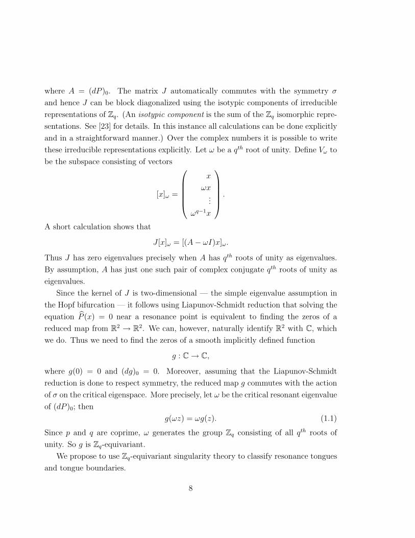
vanish. We find pocket- or flame-like regions of four q-periodic orbits in addition

to the regions with only zero or two, compare Figure 1. In addition, the tongue

boundaries contain new cusp points and in certain cases the tongue region is blunter

4

0.20.10

-0.4

-0.3

-0.2

-0.1

00.20.10

0.20.10

-0.3

-0.2

-0.1

0

-0.1

0.20.10

-0.3

-0.2

-0.1

0

-0.1

0 0.1 0.2 0.3

-0.6

-0.4

-0.2

0

0.2

0 0.1 0.2 0.3

Figure 1: Resonance tongues with pocket- or flame-like phenonmena near a degenerateHopf bifurcation through e2πip/q in a family depending on two complex parameters. Fixingone of these parameters at various (three) values yields a family depending on one complexparameter, with resonance tongues contained in the plane of this second parameter. Asthe first parameter changes, these tongue boundaries exhibit cusps (middle picture), andeven become disconnected (rightmost picture). The small triangle in the rightmost pictureencloses the region of parameter values for which the system has four q-periodic orbits.These phenomena are explained in Section 5.

than in the nondegenerate case. These results are described in detail in Section 5, also

compare Figure 2. Section 6 is devoted to concluding remarks and further questions.

Related Work

The geometric complexity of resonance domains has been the subject of many studies

of various scopes. Some of these, like the present paper, deal with quite universal

problems while others restrict to interesting examples. As opposed to this paper, often

normal form theory is used to obtain information about the nonlinear dynamics. In

the present context the normal forms automatically are Zq-equivariant.

5

Chenciner’s degenerate Hopf bifurcation. In [18, 19, 20] Chenciner considers

a 2-parameter unfolding of a degenerate Hopf bifurcation. Strong resonances to some

finite order are excluded in the ‘rotation number’ ω0 at the central fixed point. In

[20] for sequences of ‘good’ rationals pn/qn tending to ω0, corresponding periodic

points are studied with the help of Zqn-equivariant normal form theory. For a further

discussion of the codimension k Hopf bifurcation compare Broer and Roussarie [11].

The geometric program of Peckam et al. The research program reflected in

[29, 30, 33, 34] views resonance ‘tongues’ as projections on a ‘traditional’ parameter

plane of (saddle-node) bifurcation sets in the product of parameter and phase space.

This approach has the same spirit as ours and many interesting geometric properties

of ‘resonance tongues’ are discovered and explained in this way. We note that the

earlier result [32] on higher order degeneracies in a period-doubling uses Z2 equivariant

singularity theory.

Particularly we like to mention the results of [34] concerning a class of oscillators

with doubly periodic forcing. It turns out that these systems can have coexistence of

periodic attractors (of the same period), giving rise to ‘secondary’ saddle-node lines,

sometimes enclosing a flame-like shape. In the present, more universal, approach we

find similar complications of traditional resonance tongues, compare Figure 2 and its

explanation in Section 5.

Related work by Broer et al. In [14] an even smaller universe of annulus maps

is considered, with Arnold’s family of circle maps as a limit. Here ‘secondary’ phe-

nomena are found that are similar to the ones discussed presently. Indeed, apart

from extra saddle-node curves inside tongues also many other bifurcation curves are

detected.

We like to mention related results in the reversible and symplectic settings re-

garding parametric resonance with periodic and quasi-periodic forcing terms by Af-

sharnejad [1] and Broer et al. [3, 4, 7, 8, 9, 10, 12, 13, 15]. Here the methods use

Floquet theory, obtained by averaging, as a function of the parameters.

Singularity theory (with left-right equivalences) is used in various ways. First of all

it helps to understand the complexity of resonance tongues in the stability diagram. It

turns out that crossing tongue boundaries, which may give rise to instability pockets,

6

are related to Whitney folds as these occur in 2D maps. These problems already occur

in the linearized case of Hill’s equation. A question is whether these phenomena can

be recovered by methods as developed in the present paper. Finally, in the nonlinear

cases, application of Z2- and D2-equivariant singularity theory helps to get dynamical

information on normal forms.

Finding Resonance Tongues

Our method for finding resonance tongues — and tongue boundaries — proceeds as

follows. Find the region in parameter space corresponding to points where the map

P has a q-periodic orbit; that is, solve the equation P q(x) = x. Using a method due

to Vanderbauwhede (see [37, 38]), we can solve for such orbits by Liapunov-Schmidt

reduction. More precisely, a q-periodic orbit consists of q points x1, . . . , xq where

P (x1) = x2, . . . , P (xq−1) = xq, P (xq) = x1.

Such periodic trajectories are just zeroes of the map

P (x1, . . . , xq) = (P (x1)− x2, . . . , P (xq)− x1).

Note that P (0) = 0, and that we can find all zeroes of P near the resonance point by

solving the equation P (x) = 0 by Liapunov-Schmidt reduction. Note also that the

map P has Zq symmetry. More precisely, define

σ(x1, . . . , xq) = (x2, . . . , xq, x1).

Then observe thatPσ = σ P .

At 0, the Jacobian matrix of P has the block form

J =

A −I 0 0 · · · 0 0

0 A −I 0 · · · 0 0...

0 0 0 0 · · · A −I−I 0 0 0 · · · 0 A

7

where A = (dP )0. The matrix J automatically commutes with the symmetry σ

and hence J can be block diagonalized using the isotypic components of irreducible

representations of Zq. (An isotypic component is the sum of the Zq isomorphic repre-

sentations. See [23] for details. In this instance all calculations can be done explicitly

and in a straightforward manner.) Over the complex numbers it is possible to write

these irreducible representations explicitly. Let ω be a qth root of unity. Define Vω to

be the subspace consisting of vectors

[x]ω =

x

ωx...

ωq−1x

.

A short calculation shows that

J [x]ω = [(A− ωI)x]ω.

Thus J has zero eigenvalues precisely when A has qth roots of unity as eigenvalues.

By assumption, A has just one such pair of complex conjugate qth roots of unity as

eigenvalues.

Since the kernel of J is two-dimensional — the simple eigenvalue assumption in

the Hopf bifurcation — it follows using Liapunov-Schmidt reduction that solving the

equation P (x) = 0 near a resonance point is equivalent to finding the zeros of a

reduced map from R2 → R2. We can, however, naturally identify R2 with C, which

we do. Thus we need to find the zeros of a smooth implicitly defined function

g : C→ C,

where g(0) = 0 and (dg)0 = 0. Moreover, assuming that the Liapunov-Schmidt

reduction is done to respect symmetry, the reduced map g commutes with the action

of σ on the critical eigenspace. More precisely, let ω be the critical resonant eigenvalue

of (dP )0; then

g(ωz) = ωg(z). (1.1)

Since p and q are coprime, ω generates the group Zq consisting of all qth roots of

unity. So g is Zq-equivariant.

We propose to use Zq-equivariant singularity theory to classify resonance tongues

and tongue boundaries.

8

2 Zq Singularity Theory

In this section we develop normal forms for the simplest singularities of Zq-equivariant

maps g of the form (1.1). To do this, we need to describe the form of Zq-equivariant

maps, contact equivalence, and finally the normal forms.

The Structure of Zq Equivariant Maps. We begin by determining a unique

form for the general Zq-equivariant polynomial mapping. By Schwarz’s theorem [23]

this representation is also valid for C∞ germs.

Lemma 2.1 Every Zq-equivariant polynomial map g : C→ C has the form

g(z) = K(u, v)z + L(u, v)zq−1, (2.1)

where u = zz, v = zq + zq, and K,L are uniquely defined complex-valued function

germs.

Proof: It is known that every real-valued Zq-invariant polynomial h : C → R is a

function of u, v, w where w = i(zq − zq). Since

w2 = 4uq − v2,

it follows that invariant polynomials can be written uniquely in the form

h(z) = A(u, v) +B(u, v)w. (2.2)

Similarly, every Zq-equivariant polynomial mapping g : C → C is well known to

have the form

g(z) = K(z)z + L(z)zq−1,

where K and L are complex-valued invariant functions. Since

w = iv − 2izq and w = 2izq − iv

it follows thatwz = ivz − 2iuzq−1

wzq−1 = 2iuq−1z − ivzq−1.(2.3)

9

Thus we can assume that K and L are complex-valued invariant functions that are

independent of w.

Let Eu,v be the space of complex-valued map germs depending on u and v. Then

(2.1) implies that we can identify Zq-equivariant germs g with pairs (K,L) ∈ E2u,v.

When finding period q points, we are led by Liapunov-Schmidt reduction to a

map g that has the form (2.1) and satisfies K(0) = 0. By varying two parameters we

can guarantee that K(0) ∈ C can vary arbitrarily in a neighborhood of 0.

Zq Contact Equivalences. Singularity theory approaches the study of zeros of

a mapping near a singularity by implementing coordinate changes that transform

the mapping to a ‘simple’ normal form and then solving the normal form equation.

The kinds of transformations that preserve the zeros of a mapping are called con-

tact equivalences. More precisely, two Zq-equivariant germs g and h are Zq-contact

equivalent if

h(z) = S(z)g(Z(z)), (2.4)

where Z(z) is a Zq-equivariant change of coordinates and S(z) : C → C is a real

linear map for each z that satisfies

S(γz)γ = γS(z) (2.5)

for all γ ∈ Zq. A characterization of the function S is given in Lemma A.1

Normal Form Theorems In this paper we consider two classes of normal forms —

the codimension two standard for resonant Hopf bifurcation and one more degenerate

singularity that has a degeneracy at cubic order. These singularities all satisfy the

nondegeneracy condition L(0) 6= 0; we explore this case first.

Theorem 2.2 Suppose that

h(z) = K(u, v)z + L(u, v)zq−1

where K(0, 0) = 0.

q ≥ 5. If KuL(0, 0) 6= 0, then h is Zq contact equivalent to

g(z) = |z|2z + zq−1 (2.6)

10

with universal unfolding

G(z, σ) = (σ + |z|2)z + zq−1. (2.7)

q = 4. Let a = |Ku(0, 0)/L(0, 0)|. If L(0, 0) 6= 0 and a 6= 0, 1, then h is Z4 contact

equivalent to

g(z) = auz + z3

where 0 < a < 1 or 1 < a is a moduli parameter. The universal unfolding of g is

G(z) = (σ + au)z + z3 (2.8)

where σ ≈ 0 is complex.

q = 3. If L(0, 0) 6= 0, then the normal form for q = 3 is

g(z) = z2,

which has codimension two, and the universal unfolding of g is

G(z) = σz + z2. (2.9)

Theorem 2.3 Suppose that

h(z) = K(u, v)z + L(u, v)zq−1

where K(0, 0) = 0 = Ku(0, 0) and q ≥ 7. If Kuu(0, 0)L(0, 0) 6= 0, then h is Zq contact

equivalent to

g(z) = |z|4z + zq−1 (2.10)

with universal unfolding

G(z, σ, τ) = (σ + τ |z|2 + |z|4)z + zq−1, (2.11)

where σ, τ ∈ C.

The proofs of Theorems 2.2 and 2.3 are given in Section A.

11

3 Resonance domains

In this section we compute boundaries of resonance domains corresponding to uni-

versal unfoldings of the form

G(z) = b(u)z + zq−1. (3.12)

By definition, the tongue boundary is the set of parameter values where local bifurca-

tions in the number of period q points take place; and, typically, such bifurcations will

be saddle-node bifurcations. For universal unfoldings of the simplest singularities the

boundaries of these parameter domains have been called tongues, since the domains

have the shape of a tongue, with its tip at the resonance point. Below we show that

our method easily recovers resonance tongues in the standard least degenerate cases.

Then, we study a more degenerate singularity and show that the usual description of

tongues needs to be broadened.

Tongue boundaries of a p : q resonance are determined by the following system

zG = 0

det(dG) = 0.(3.13)

This follows from the fact that local bifurcations of the period q orbits occur at

parameter values where the system G = 0 has a singularity, that is, where the rank

of dG is less than two. Recalling that

u = zz v = zq + zq w = i(zq − zq), (3.14)

we prove the following theorem, which is independent of the form of b(u).

Theorem 3.1 For universal unfoldings (3.12), equations (3.13) have the form

|b|2 = uq−2

bb′+ bb′ = (q − 2)uq−3

(3.15)

Proof: Begin by noting that G(z) = 0 implies that

zG(z) = bu+ zq = 0.

12

Therefore,

zq = −bu and zq = −bu.

It follows that

v = −(b+ b)u and w = −i(b− b)u.

Hence, the identity v2 + w2 = 4uq implies

|b|2 = uq−2,

which is the first result to be shown.

Next we compute det(dG) = 0 by recalling that in complex coordinates

det(dG) = |Gz|2 − |Gz|2.

Observe that

|Gz|2 = (b+ b′u)(b+ b′u)

= |b|2 + (bb′+ bb′)u+ |b′|2u2

and

|Gz|2 = (b′z2 + (q − 1)zq−2)(b′z2 + (q − 1)zq−2)

= |b′|2u2 − (q − 1)(bb′+ bb′)u+ (q − 1)2uq−2.

Therefore,

0 = det(dG) = |b|2 + q(bb′+ bb′)u− (q − 1)2uq−2. (3.16)

The second equation in (3.15) now follows from (3.16) by applying the first equation

in (3.15), which has already been proved.

We now use (3.15) to determine tongue boundaries for the universal unfoldings

classified in Theorems 2.2 and 2.3.

4 Nondegenerate Cases: Resonance Tongues

Here we recover several classical results on the geometry of resonance tongues, in the

present context of Hopf bifurcation. To begin, we discuss weak resonances q ≥ 5,

13

where a q2− 1 cusp forms the tongue-tip and where the concept of resonance tongue

remains unchallenged. Note that similar tongues are found in the Arnold family of

circle maps [2], also compare Broer, Simo and Tatjer [14]. Then, we consider the

strong resonances q = 3 and q = 4, where we again recover known results on the

shape of the resonance domain. For a more complete discussion of the dynamics near

these resonance points, see Takens [35] or Arnold [2].

The Nondegenerate Singularity when q ≥ 5

We first investigate the nondegenerate case q ≥ 5 given in (2.7). Here

b(u) = σ + u

where σ = µ+ iν. We shall compute the tongue boundaries in the (µ, ν)-plane in the

parametric form µ = µ(u), ν = ν(u), where u ≥ 0 is a local real parameter.

Short computations show that

|b|2 = (µ+ u)2 + ν2

bb′+ bb′ = 2(µ+ u).

Then Theorem 3.1 gives us the following parametric representation of the tongue

boundaries:

µ = −u+q − 2

2uq−3

ν2 = uq−2 − (q − 2)2

4u2(q−3).

In this case the tongue boundaries at (µ, ν) = (0, 0) meet in the familiar q−22

cusp

ν2 ≈ (−µ)q−2. (4.17)

It is to this and similar situations that the usual notion of resonance tongue applies:

inside the sharp tongue a pair of period q orbits exists and these orbits disappear in

a saddle-node bifurcation at the boundary.

14

The Nondegenerate Singularity when q = 4

In this case by (2.8) we have that

b(u) = σ + au,

where with a a modulus parameter such that a > 0 and a 6= 1. Short computations

show that

|b|2 = (µ+ au)2 + ν2

bb′+ bb′ = 2a(µ+ au).

¿From (3.15) we obtain

µ =1− a2

au

ν2 =a2 − 1

a2u2.

These equations again give a parametric description of the resonance domain in the

(µ, ν) plane. When a > 1 we find tongue boundaries formed by the lines

µ = ±√a2 − 1ν.

So the tongues bound a wedge approaching a half line as a approaches 1. When

0 < a < 1 there are no tongue boundaries — period 4 points exist for all values of

(µ, ν).

The Nondegenerate Singularity when q = 3

In this case we have

b = σ.

Again we recover the familiar result that no tongues exist, but that period 3 points

exist for all values of (µ, ν).

More precisely, there is a period 3 trajectory, corresponding to a solution of (2.9),

for every σ 6= 0. To verify this point, set σ = reiθ. Then, set z = e−iθ/3y in (2.9)

obtaining:

ry + y2 = 0,

where r is real and positive. It follows that y = −r is a nonzero solution.

15

5 Degenerate Singularities when q ≥ 7

Tongue boundaries in the degenerate case

The next step is to analyze a more degenerate case, namely, the singularity

g(z) = u2z + zq−1,

when q ≥ 7. We recall from (2.11) that a universal unfolding of g is given by

G(z) = b(u)z + zq−1, where

b(u) = σ + τu+ u2. (5.18)

Here σ and τ are complex parameters, which leads to a real 4-dimensional parameter

space. As before, we set σ = µ + iν and consider how the tongue boundaries in the

(µ, ν)-plane depend on the complex parameter τ . In this discussion, we calculate the

tongue boundaries with computer assistance, using the parametric forms of µ and

ν given by Theorem 5.2 below. We will see that a new complication occurs in the

tongue boundaries for certain τ , namely, cusp bifurcations occur at isolated points

of the fold (saddle-node) lines. The interplay of these cusps is quite interesting and

challenges some of the traditional descriptions of resonance tongues when q = 7 and

presumably for q ≥ 7.

We recall that the tongue boundaries are determined by equations (3.13). For

the specific choice (5.18) for b it follows that the solution of these equations is the

discriminant set

DP = {(σ, τ) ∈ C× C | P (u, σ, τ) =∂P

∂u(u, σ, τ) = 0, for some u ∈ R}

of the polynomial P , defined by

P (u, σ, τ) = (u2 + τu+ σ)(u2 + τu+ σ)− uq−2.

Putting τ = α + iβ and σ = µ + iν, with α, β, µ, ν ∈ R, we obtain the following

expression for the family P :

P (u, α, β, µ, ν) = u4 − uq−2 + 2αu3 + (α2 + β2 + 2µ)u2+

2(αµ+ βν)u+ (µ2 + ν2).(5.19)

16

We try to obtain a parametrization of DP by solving the system of equations

P (u, α, β, µ, ν) =∂P

∂u(u, α, β, µ, ν) = 0, (5.20)

for µ and ν. This gives us a solution of the form

(µ, ν) = (µ(u, α, β), ν(u, α, β)),

which defines a curve in the (µ, ν)-plane, for fixed (α, β).

To this end we consider the solution set of (5.20) as a perturbation of the solution

set of the system

P0(u, α, β, µ, ν) =∂P0

∂u(u, α, β, µ, ν) = 0,

where

P0(u, σ, τ) = (u2 + τu+ σ)(u2 + τu+ σ) = P (u) + uq−2.

Lemma 5.1 The discriminant set of P0 is the hypersurface in R4 parametrized by

Γ0 : R× R2 → R4, with Γ0(u, α, β) = (α, β, µ0(u, α, β), ν0(u, α, β)) defined by

µ0(u) = −u(α + u),

ν0(u) = −βu.(5.21)

Proof: First we observe that every root of P0(u, σ, τ) = 0 has multiplicity at

least two, so P0(u, σ, τ) = 0 implies∂P0

∂u(u, σ, τ) = 0. Now P0(u, τ, σ) = 0 implies

µ = µ0(u, α, β) and ν = ν0(u, α, β), with µ0 and ν0 as in (5.21). This completes the

proof.

Theorem 5.2 The discriminant set of P is the union of the two hypersurfaces D±Pin R4 parametrized by Γ± : R× R2 → R4, with Γ± of the form

Γ±(u, α, β) = (α, β, µ0(u, α, β) +M±(u, α, β), ν0(u, α, β) +N±(u, α, β) ),

with

M±(u, α, β) =(q − 2)uq−3(α + 2u)± βu(q−2)/2

√

4D(u, α, β)− (q − 2)2uq−4

2D(u, α, β),

N±(u, α, β) =(q − 2)βuq−3 ∓ (α + 2u)u(q−2)/2

√

4D(u, α, β)− (q − 2)2uq−4

2D(u, α, β),

(5.22)

where

D(u, α, β) = (α + 2u)2 + β2.

17

Proof: We try to obtain a solution of (5.20) by perturbing the parametrization

(5.21) by putting

µ = µ0(u, α, β) +M,

ν = ν0(u, α, β) +N.

Plugging this into (5.20) yields the following system of equations for M and N :

M2 +N2 − uq−2 = 0,

2αM + 2βN + 4Mu− (q − 2)uq−3 = 0.

This system has two pairs of real solutions (M±(u, α, β), N±(u, α, β)) defined by

(5.22).

In the next subsection this parametrization is used to obtain pictures of the resonance

regions for various values of τ = α + iβ.

Degenerate tongue boundaries when q = 7.

Below we explore the tongue boundaries numerically for fixed τ . Note that the

discriminant set DP is invariant under the transformation (σ, τ) 7→ (σ, τ). Thus, we

may assume that Im(τ) ≥ 0. To perform these calculations, we set τ = ρe2πiθ, where

0 ≤ θ ≤ 0.5.

We use Mathematica to plot the curves given by Theorem 5.2 for various values

of τ . Fixing ρ = 0.1 we choose several representative values of θ ∈ (0, 0.5). In

Figure 2, left column, we consider θ = 0.01, 0.10 and 0.30, thereby traversing the

first quadrant, and see a resonance tongue that begins to rotate and bend. Inside the

cusped region there are two (locally defined) period 7 trajectories that annihilate each

other in a saddle-node bifurcation as the tongue boundary is crossed. This description

is consistent with the description of resonance tongues in the least degenerate case.

However, this description changes as τ nears the negative real axis.

In Figure 2, middle column, we consider θ = 0.42 and 0.44. At θ = 0.44, apart

from further bending of the tongue, we see that a small triangular ‘pocket’ or ‘flame’

has emerged from one of the tongue boundaries. This pocket is defined by two

cusps and a crossing of the boundary curve. Inside the pocket region, there are four

18

trajectories of period 7 points. The bending continues at θ = 0.45 where the two

cusps approach the tongue boundary, see Figure 2, right column.

Finally, we see in Figure 2 that by θ = 0.48, the two cusps and the tongue tip

have formed a triangle that has detached from the rest of the boundary. In the 4-

dimensional (σ, τ) parameter space, this geometry is reminiscent of catastrophes like

the swallowtail or elliptic umbilic — but in a Zq-equivariant setting. For τ near the

negative real axis this analysis refers to the boundary of the pocket region shown in

Figure 2 (right column) that surrounds the region of the four period 7 trajectories.

For this part of the boundary we find the expected thin resonance ‘tongue’ — but

that ‘tongue’ does not refer to the boundary between regions where period 7 points

exist and regions where they do not. In the next section we show that the four period

7 points occur for α arbitrarily close to 0.

19

-1.5 -1 -0.5 0

-0.3-0.2-0.1

00.10.2

-1.5 -1 -0.5 0

-0.8

-0.6

-0.4

-0.2

0-1.5 -1 -0.5 0

-0.8

-0.6

-0.4

-0.2

0

-0.6 -0.4 -0.2 0

-1

-0.8

-0.6

-0.4

-0.2

0-0.6 -0.4 -0.2 0

0.20.10

-0.4

-0.3

-0.2

-0.1

00.20.10

0.20.10

-0.3

-0.2

-0.1

0

-0.1

0.20.10

-0.3

-0.2

-0.1

0

-0.1

0.30.20.10

-0.2

-0.1

0

-0.1

0.30.20.10

-0.2

-0.1

0

-0.1

0 0.1 0.2 0.3

-0.6

-0.4

-0.2

0

0.2

0 0.1 0.2 0.3

τ-plane1

2

3

45

67

1

2

3

4

5

6

7

Figure 2: Top: the τ -plane. Frames 1–7: Resonance tongues in the σ-plane for variousvalues of τ = 0.1 e2πiθ. (1) θ = 0.01, (2) θ = 0.10, (3) θ = 0.30, (4) θ = 0.42, (5) θ = 0.44,(6) θ = 0.45, (7) θ = 0.48.

20

Four q-periodic orbits

Our pictures of the resonance regions for various values of τ suggest the existence of

a small ‘triangle’ in the σ-plane with interior points corresponding to the occurrence

of four real roots near 0 of the equation P (u, σ, τ) = 0. This triangle emerges for

τ -values near the negative real axis. In this section we show that this region exists

for τ -values arbitrarily near the origin. We do so by constructing a smooth curve in

parameter space, emerging from the origin, such that the equation P (u, σ, τ) = 0 has

four real roots near u = 0 for parameter values (σ, τ) on this curve.

To this end we observe that the ‘spine’ of the resonance region is the curve

parametrized by (5.21). This spine corresponds to parameter values (σ, τ) for which

the polynomial P0(u, σ, τ) has two double zeros. Indeed, a simple computation shows

that

P0(u,−αt− t2,−βt, α, β) = (u− t)2(

(u+ t+ α)2 + β2)

. (5.23)

We now define a curve in parameter space by making t and β dependent on α,

in such a way that four real zeros occur for parameters on this curve. Since our

experiments indicate that four small real roots occur for τ near the negative real axis

we put β = 0, and expect four real roots (where we have to restrict to α < 0 if q

is odd). Furthermore, the triangle enclosing σ-values for which four small real roots

are observed shrinks to size 0 as τ tends to 0. Therefore, our second guess is t = α2.

(In fact, we first tried t = α, but the corresponding curve tends to 0 via the region

of two small real roots).

Summarizing, we consider the one parameter family p(u, α) of polynomials in u,

defined by

p(u, α) = P (u,−α3 − α4,−α4, α, 0). (5.24)

In view of (5.23), this polynomial satisfies

p(u, α) = (u− α2 )2(u+ α + α2 )2 − uq−2.

Theorem 5.3

1. For sufficiently small α the polynomial p(·, α) has a pair u±(α) of distinct real

zeros near 0 ∈ R, satisfying

u±(α) = α2 ± αq−3 +O(αq−2), (5.25)

21

2. Moreover, for sufficiently small α there is an other pair U±(α) of distinct real zeros

near 0 ∈ R, satisfying

U±(α) = −α− α2 ± |α|q−4

2 +O(|α|q−3

2 ), (5.26)

for q odd, and α ≤ 0, and

U±(α) = −α− α2 ± αq−4

2 +O(αq−2

2 ), (5.27)

for q even.

The proof is contained in Appendix B.

Corollary 5.4 There are parameter values (σ, τ) arbitrarily near (0, 0) ∈ C× C for

which four period q trajectories exist.

Four Dimensional Geometric Structure

We derived the parametrization (5.22) of the discriminant set DP of the family P ,

given by (5.19). Using this parametrization, we obtained cross-sections of this singular

surface DP ; See Figure 2. In this section we show that DP is the pull-back (under a

singular map) of the product of the swallowtail and the real line.

To this end, consider the discriminant set of the model family Q : R4 → R, defined

by

Q(u, κ, λ, %, α) = u4 − uq−2 + 2αu3 + %u2 + λu+ κ. (5.28)

In fact, DP is the pull-back of DQ under the singular map ψ : R4 → R4, defined by

ψ(α, β, µ, ν) = (µ2 + ν2, αµ+ βν, α2 + β2 + 2µ, α, ). (5.29)

We note in passing that the map ψ : R4 → R4, given by (5.29), has rank 2 at 0 ∈ R4.

Its singular set is given by

S(ψ) = {(α, β, µ, ν) | β2µ− αβν + ν2 = 0},

and is diffeomorphic to the product of the real line and the Whitney umbrella W =

{(β, µ, ν) | β2µ+ ν2 = 0}. See also Figure 3.

22

β

µ

ν

Figure 3: The Whitney umbrella β2µ+ ν2 = 0.

The discriminant set DQ is the product of the real line and a swallowtail, locally

near 0 ∈ R4. This follows from the fact that Q is a versal unfolding of the function

u 7→ u4 − uq−2, which is right-equivalent to the function u4, locally near 0 ∈ R. A

universal unfolding of the latter function is Q : R× R3 → R, defined by

Q(u, κ, λ, %) = u4 + %u2 + λu+ κ.

Since the discriminant set of Q is a (standard) swallowtail-surface, it follows from

Singularity Theory that DQ is diffeomorphic to the product of the real line and this

swallowtail-surface.

To visualize DQ, we solve κ and λ from the equations

Q(u, κ, λ, %, α) =∂Q

∂u(u, κ, λ, %, α) = 0.

Thus we see that DQ is the singular surface in R4 parametrized by

(u, %, α) 7→ (κ, λ, %, α) = (−2%u−6au2−4u3+5u4, %u2+4au3+3u4−4u5, %, α), (5.30)

with (u, %, α) near (0, 0, 0) ∈ R3. In Figure 4 we depict this surface, and recognize

the swallowtail geometry.

23

α ≈ 0, % < 0 α ≈ 0, % = 0 α ≈ 0, % > 0

κ κ κ

λλ λ

Figure 4: The discriminant set of the family Q(u, κ, λ, %, α) = u4−u5 +2αu3 +%u2 +λu+κ

parametrized by (5.30), locally near 0 ∈ R4. This surface is the product of the real line anda swallowtail, near 0 ∈ R4. Top row: Cross-sections of DQ with planes (w,α) = (w0, α0).Bottom row: Cross-sections of DQ with hyperplanes α = α0.

Concluding Remarks for the Case q ≥ 7.

First, from the above description it is clear that the resonance domain generally is

more complicated than the familiar tongue. Globally speaking the resonance domain

is bounded by a saddle-node curve: ‘inside’ at least two q-periodic solutions exist

that annihilate each other at the outer boundary. The inner boundary again consists

of saddle-node curves, that meet at a cusp or at the ‘tongue tip’. Inside the pocket-

or flame-like triangular region four q-periodic orbits exist.

Second, the sharpness of the ‘tongue’ at the resonance (µ, ν) = (0, 0) in the central

24

singularity τ = 0 can be computed directly from equations (5.22); it is

ν ≈ (−µ)q−2

4 , (5.31)

which is a q−24

cusp. Note that the degenerate cusp is blunter than the q−22

cusp we

found in the standard nondegenerate case q ≥ 5, see (4.17). In the present unfolding,

for τ 6= 0 the ‘tongue’ tip will be a nondegenerate q−22

cusp, where the leading

coefficient depends on the value of τ.

Third, we comment on the scale of the present phenomena. From the numerical

experiments, we see that for θ near 0.5, the description of the local geometry covers

two scales — both of which are local. The secondary cusps and pockets or flames occur

on a small scale. On a larger scale the resonance domain looks like a rather blunt

cusp. These conclusions challenge the standard view of a sharp resonance tongue

when q ≥ 5. Compare this behavior to the case where τ is in the first quadrant, that

is, where 0 < θ < 0.25. In this case, the tongues near the degeneracy τ = 0 behave

very much like tongues in the nondegenerate case.

6 Conclusions

We have developed a method, based on Liapunov-Schmidt reduction and Zq equiv-

ariant singularity theory, to find period q resonance tongues in a Hopf bifurcation for

dissipative maps. We recovered the standard nondegenerate results [2, 35], but also

illustrated the method on the degenerate case q ≥ 7. We now address various issues

related to these methods and results, that we aim to pursue in future research.

First we like to get a better understanding of the way in which the four dimen-

sional geometry, in particular the swallowtail catastrophe and the Whitney umbrella,

determine the possible pockets or flames in the resonance tongues. Related to this,

we like to address the question of strong resonances q ≤ 6 in the degenerate case;

the present method can be adapted to these cases. To compute and visualize higher

dimensional resonance domains we envision applying a combination of analytic and

experimental techniques.

Second, our methods can be extended to other contexts, in particular, to cases

where extra symmetries, including time reversibility, are present. This holds both for

25

Liapunov-Schmidt reduction and Zq equivariant singularity theory. In this respect

Golubitsky, Marsden, Stewart, and Dellnitz [21], Knobloch and Vanderbauwhede [25,

27], and Vanderbauwhede [36] are helpful.

Third, there is the issue of how to apply our results to a concrete family of

dynamical systems. Golubitsky and Schaeffer [22] describe methods for obtaining the

Taylor expansion of the reduced function g(z) in terms of the Poincare map P and

its derivatives. These methods may be easier to apply if the system is a periodically

forced second order differential equation, in which case the computations again may

utilize parameter dependent Floquet theory.

For numerical experiments our results may be helpful in the following way. If the

third order ‘Hopf coefficients’ vanish at a specific parameter value, then, for nearby

parameter values, we expect resonance tongues as described in Section 5.

Finally, in this paper we have studied only degeneracies in tongue boundaries.

It would also be interesting to study low codimension degeneracies in the dynamics

associated to the resonance tongues. Such a study will require tools that are more

sophisticated than the singularity theory ones that we have considered here.

Acknowledgments We would like to thank Vincent Naudot, Michael Sevryuk,

Floris Takens, and Andre Vanderbauwhede for their help and suggestions. The re-

search of MG was supported in part by NSF Grant DMS-0071735.

References

[1] Z. Afsharnejad. Bifurcation geometry of Mathieu’s equation. Indian J. Pure

Appl. Math. 17 (1986) 1284–1308.

[2] V.I. Arnold, Geometrical Methods in the Theory of Ordinary Differential Equa-

tions, Springer-Verlag 1982.

[3] H.W. Broer, S.-N. Chow, Y. Kim & G. Vegter, A normally elliptic Hamiltonian

bifurcation, ZAMP 44, (1993), 389–432.

26

[4] H.W. Broer, S.-N. Chow, Y. Kim & G. Vegter, The Hamiltonian double-zero

eigenvalue, In: W.F. Langford, W. Nagata (eds.), Normal Forms and Homoclinic

Chaos, Waterloo 1992 , Fields Institute Communications, 4, (1995), 1–19.

[5] H.W. Broer, I. Hoveijn & M. van Noort, A reversible bifurcation analysis of the

inverted pendulum, Physica D , 112, (1998), 50–63.

[6] H.W. Broer, I. Hoveijn, M. van Noort & G. Vegter, The inverted pendulum: a

singularity theory approach, Journ. Diff. Eqns. 157, (1999), 120–149.

[7] H.W. Broer, I. Hoveijn, G.A. Lunter & G. Vegter, Resonances in a Spring–

Pendulum: algorithms for equivariant singularity theory, Nonlinearity, 11(5),

(1998), 1–37.

[8] H.W. Broer, I. Hoveijn, G.A. Lunter & G. Vegter, Bifurcations in Hamiltonian

systems: Computing singularities by Grobner bases. To appear Springer LNM,

2002

[9] H.W. Broer and M. Levi. Geometrical aspects of stability theory for Hill’s equa-

tions, Arch. Rational Mech. Anal. 131 (1995) 225–240.

[10] H.W. Broer, G.A. Lunter & G. Vegter, Equivariant singularity theory with dis-

tinguished parameters, two case studies of resonant Hamiltonian systems, Phys-

ica D , 112, (1998), 64–80.

[11] H.W. Broer and R. Roussarie, Exponential confinement of chaos in the bifur-

cation set of real analytic diffeomorphisms. In H.W. Broer, B. Krauskopf and

G. Vegter (Eds.), Global Analysis of Dynamical Systems, Festschrift dedicated to

Floris Takens for his 60th birthday. pp. 167–210. Bristol and Philadelphia IOP,

2001. ISBN 0 7503 0803 6.

[12] H.W. Broer and C. Simo. Hill’s equation with quasi-periodic forcing: resonance

tongues, instability pockets and global phenomena. Bol. Soc. Bras. Mat. 29 1998

253–293.

[13] H.W. Broer and C. Simo. Resonance tongues in Hill’s equations: a geometric

approach. J. Diff. Eqns. 166 (2000) 290–327.

27

[14] H.W. Broer, C. Simo, and J.-C. Tatjer. Toward global models near homoclinic

tangencies of dissipative diffeomorphisms. Nonlinearity 11 (1998) 667–770.

[15] H.W. Broer and G. Vegter. Bifurcational aspects of parametric resonance. Dy-

namics Reported, New Series 1 (1992) 1–51.

[16] H.W. Broer, G. Vegter, et al., Pulling back a Swallowtail through a Whitney

Umbrella. In preparation.

[17] J.W. Bruce and P.J. Giblin. Curves and Singularities. Cambridge University

Press, 1984.

[18] A. Chenciner, Bifurcations de points fixes elliptiques, I. Courbes invariantes,

Publ. Math. IHES 61 (1985), 67–127.

[19] A. Chenciner, Bifurcations de points fixes elliptiques, II. Orbites periodiques et

ensembles de Cantor invariants. Invent. Math. 80(1) (1985), 81–106.

[20] A. Chenciner, Bifurcations de points fixes elliptiques, III. Orbites periodiques de

“petites” periodes et elimination resonnantes des couples de courbes invariantes,

Publ. Math. IHES 66 (1988), 5–91.

[21] M. Golubitsky, J.E. Marsden, I. Stewart and M. Dellnitz. The constrained

Liapunov-Schmidt procedure and periodic orbits. In: J. Chadam, M. Golubitsky,

W. Langford and B. Wetton (Eds.), Pattern Formation: Symmetry Methods and

Applications, Fields Institute Communications, Vol. 4, 81–127, American Math-

ematical Society, Providence, 1996.

[22] M. Golubitsky and D.G. Schaeffer. Singularities and Groups in Bifurcation The-

ory: Vol. I , Applied Mathematical Sciences 51. Springer-Verlag, New York, 1985.

[23] M. Golubitsky, I.N. Stewart and D.G. Schaeffer. Singularities and Groups in

Bifurcation Theory: Vol. II. Applied Mathematical Sciences 69, Springer-Verlag,

New York, 1988.

[24] A. Hummel. Bifurcations of periodic points. PhD Thesis, University of Gronin-

gen, 1979.

28

[25] J. Knobloch and A. Vanderbauwhede. Hopf bifurcation at k-fold resonances in

equivariant reversible systems. In: P. Chossat (Ed.), Dynamics. Bifurcation and

Symmetry. New Trends and New Tools. NATO ASI Series C, Vol. 437, 167–179,

Kluwer Acad. Publ., Dordrecht, 1994.

[26] J. Knobloch and A. Vanderbauwhede. Hopf bifurcation at k-fold resonances in

conservative systems. In: H.W. Broer, S.A. van Gils, I. Hoveijn and F. Takens

(Eds.), Nonlinear Dynamical Systems and Chaos. Progress in Nonlinear Differ-

ential Equations and Their Application, Vol. 19, 155–170, Birkhauser Verlag,

Basel-Boston-Berlin, 1996.

[27] J. Knobloch and A. Vanderbauwhede. A general method for periodic solutions

in conservative and reversible systems. J. Dynamics Diff. Eqns. 8 (1996) 71–102.

[28] B. Krauskopf. Bifurcation sequences at 1:4 resonance: an inventory. Nonlinearity

7 (1994) 1073–1091.

[29] R.P. McGehee and B.B. Peckham, Determining the global topology of reso-

nance surfaces for periodically forced oscillator families. In W.F. Langford and

W. Nagata (eds.), Normal Forms and Homoclinic Chaos. Fields Institute Com-

munications 4 AMS 1995, 233–254.

[30] R.P. McGehee and B.B. Peckham, Arnold flames and resonance surface folds,

Int. J. Bifurcations and Chaos 6(2) (1996) 315–336.

[31] S.E. Newhouse, J. Palis, and F. Takens. Bifurcation and stability of families of

diffeomorphisms. Publ Math. I.H.E.S 57 (1983) 1–71.

[32] B.B. Peckham and I.G. Kevrekidis, Period doubling with higher-order degenera-

cies, SIAM J. Math. Anal. 22(6) (1991) 1552–1574.

[33] B.B. Peckham, C.E. Frouzakis and I.G. Kevrekidis, Bananas and banana splits:

a parametric degeneracy in the Hopf bifurcation for maps, SIAM. J. Math. Anal.

26(1) (1995) 190–217.

[34] B.B. Peckham and I.G. Kevrekidis, Lighting Arnold flames: Resonance in dou-

bly forced periodic oscillators. Nonlinearity 15 (2002) 405–428.

29

[35] F. Takens, Forced oscillations and bifurcations. In Applications of Global Analy-

sis I. Communications of the Mathematical Insitute Rijksuniversiteit Utrecht 3

(1974), 1–59.

Reprinted in H.W. Broer, B. Krauskopf and G. Vegter (eds.), Global Analysis of

Dynamical Systems, Festschrift dedicated to Floris Takens for his 60th birthday,

Institute of Physics Publishing 2001, 1–62.

[36] A. Vanderbauwhede. Hopf bifurcation for equivariant conservative and time-

reversible systems. Proc. Royal Soc. Edinburgh 116A (1990) 103–128.

[37] A. Vanderbauwhede. Branching of periodic solutions in time-reversible systems.

In: H.W. Broer and F. Takens (Eds.), Geometry and Analysis in Non-Linear

Dynamics. Pitman Research Notes in Mathematics, Vol. 222 97–113, Pitman,

London, 1992.

[38] A. Vanderbauwhede. Subharmonic bifurcation at multiple resonances. In: Pro-

ceedings of the Mathematics Conference (S. Elaydi et al., eds) World Scientific,

Singapore, 2000, 254–276.

A Proofs of the Singularity Theory Theorems

This section divides into three parts. In the short first part we complete our descrip-

tion of Zq-equivariant contact equivalence by describing the structure of the mappings

S satisfying the equivariance condition (2.5). The second part is devoted to deriving

explicit generators for the tangent space of a Zq-equivariant mapping under contact

equivalence. The last part uses the general ‘tangent space constant’ and ‘universal

unfolding theorems’ of equivariant singularity theory [22, 23] to derive the normal

form theorems in Section 2.

Lemma A.1 Every map germ S(z) : C→ C that satisfies (2.5) has the form

S(z)y = α(u, v, w)y + (ϕ(u, v, w)z2 + ψ(u, v, w)zq−2)y

where α, ϕ, ψ are complex-valued and have the form (2.2).

30

Proof: A real linear map from C to C can be written as y 7→ αy + βy where

α, β ∈ C. It follows that the linear map S(z) has the form

S(z)(y) = α(z)y + β(z)y.

The equivariance condition (2.5) implies that

α(γz) = α(z) and β(γz) = γ2β(z).

The equivariance condition on β(z) implies that

β(z) = ϕ(z)z2 + ψ(z)zq−2,

where ϕ and ψ are complex Zq-invariant functions. We may assume that α, ϕ, ψ are

functions of u, v, w that are affine linear in w. See (2.2).

Of course, since Z(z) is Zq-equivariant, it has the form

Z(z) = ζ(z)z + ξ(z)zq−1

where ζ and ξ are complex Zq-invariant functions. Thus Zq contact equivalences are

determined by five complex-valued Zq-invariant functions α, ϕ, ψ, ζ, ξ.

The Zq Tangent Space. Equivariant singularity theory has two main theorems

that are used to determine Zq-equivariant normal forms. Let T (g) be the ‘tangent

space’ of g, which we define formally in Definition A.2. The tangent space constant

theorem states that if p : C→ C is Zq-equivariant and

T (g + tp) = T (g)

for all t ∈ R, then g + p is contact equivalent to g. The universal unfolding theorem

states that if V = R{p1(z), . . . , pk(z)} is a complementary subspace to T (g) in the

space of germs of Zq-equivariant mappings, then

G(z, α1, . . . , αk) ≡ g(z) + α1p1(z) + · · ·+ αkpk(z)

is a universal unfolding of g.

The tangent space to a Zq-equivariant germ g is generated by infinitesimal versions

of S and Z in (2.4), as follows.

31

Definition A.2 The tangent space of g(z) consists of all germs of the form

d

dtgt(z)

∣

∣

∣

∣

t=0

where gt(z) is a one-parameter family of germs that are contact equivalent to g(z)

and g0 = g.

The assumption that gt is a one-parameter family of germs that are contact equiv-

alent to g means that

gt(z) = S(z, t)g(Z(z, t))

where S and Z satisfy the appropriate equivariance conditions. The assumption that

g0 = g allows us to assume that S(z, 0) = 1 and Z(z, 0) = z. When computing

the tangent space of g, linearity implies that we need consider only the deformations

defined by the five invariant functions functions in the general equivalence — three

coming from S(z) and two from Z(z). Thus

Lemma A.3 The tangent space T (g) is generated by 16 generators with coefficients

that are real-valued Zq-invariant functions of u and v. The first 12 generators are

obtained by multiplying each of the following three generators by 1, w, i, and iw:

g(z) z2g(z) zq−2g(z). (A.1)

The remaining four generators are:

(dg)z(z) (dg)z(iz) (dg)z(zq−1) (dg)z(iz

q−1). (A.2)

Proof: Lemma A.1, coupled with (2.2), states that the function S is generated by

six generators with coefficients that are functions of u and v. Lemma 2.1 states that

Z is generated by two generators. Using the chain rule in the differentiation required

by Definition A.2 leads to the last four generators.

Our next task is to compute the generators of T (g) using the identification of a Zqequivariant g(z) with the pair of complex-valued functions (K(u, v), L(u, v)) ∈ E2

u,v.

Proposition A.4 Let g be identified with the pair (K,L) ∈ E2u,v where K,L are

complex-valued functions. Then, in terms of (K,L), there are 12 generators of T (g).

The first eight generators are obtained by multiplying the four generators

(K,L) (uK + vL,−uL) (uq−2L,K) (uq−1L,−uK − vL)

32

by 1 and i. The last four generators are

(2uKu + qvKv, qL+ 2uLu + qvLv)

(i(2uq−1Lv + vKv),−i(2uKv + L+ vLv))

(2quq−1Kv + vKu + (q − 1)uq−2L,K + 2quq−1Lv + vLu)

(−i(vKu + 2uq−1Lu + (q − 1)uq−2L), i(K + 2uKu + vLu))

Proof: The generators associated to multiplication by S are easiest to determine.

Just compute

g(z) = Kz + Lzq−1, z2g(z) = uKz + Lzqz, zq−2g(z) = Kzq−1 + uq−2Lz

Using zqz = vz − uzq−1, we see that these generators correspond to:

(K,L), (uK + vL,−uL), (uq−2L,K). (A.3)

To determine the generators with a w factor, use (2.3) to compute

w(K,L) = i(vK + 2uq−1L,−2uK − vL). (A.4)

Using (A.4), it follows that

w(uK + vL,−uL) = i(uvK + (v2 − 2uq)L,−2u2K − uvL)

w(uq−2L,K) = i(2uq−1K + uq−2vL,−vK − 2uq−1L).

Note that

w(uK + vL,−uL) = iv(uK + vL,−uL)− 2iu2(uq−2L,K).

Thus, using (A.3), we see that this generator is redundant. Similarly,

w(uq−2L,K) = 2iuq−2(uK + vL,−uL)− iv(uq−2L,K).

So, this generator is also redundant.

To find the tangent space generators (A.2) corresponding to Z(z), we first compute

Kz = Kuz + qKvzq−1

Kz = Kuz + qKvzq−1

33

where K = K(u, v) is Zq-invariant. Similar formulae hold for L. The tangent space

generators from domain coordinate changes are

(dg)z(ζ(z)z) and (dg)z(ξ(z)zq−1) (A.5)

where

(dg)z(y) = gz(z)y + gz(z)y.

So we compute

gz = K +Kzz + Lzzq−1

= K + (Kuz + qKvzq−1)z + (Luz + qLvz

q−1)zq−1

= K + uKu + quq−1Lv + qKvzq + Luz

q.

Also

gz = Kzz + (q − 1)Lzq−2 + Lzzq−1

= (Kuz + qKvzq−1)z + (q − 1)Lzq−2 + (Luz + qLvz

q−1)zq−1

= Kuz2 + (quKv + (q − 1)L+ uLu + qLvz

q)zq−2

The first generator from (A.5) is

(dg)z(ζz) = gzζz + gzζz

= ζ(K + uKu + quq−1Lv + qKvzq + Luz

q)z+

ζ(Kuz2 + (quKv + (q − 1)L+ uLu + qLvz

q)zq−2)z

= ζ(K + uKu + quq−1Lv + qKvzq)z + ζuLuz

q−1+

ζuKuz + ζ(quKv + (q − 1)L+ uLu + qLvzq)zq−1

= ζ(K + uKu + quq−1Lv + qvKv)z + ζu(Lu − qKv)zq−1+

ζu(Ku − qLvuq−2)z + ζ(quKv + (q − 1)L+ uLu + qvLv)zq−1,

(A.6)

using zq = v − zq and zq = v − zq. Evaluating (A.6) with ζ = 1 and ζ = i yields the

two generators

(K + 2uKu + qvKv, (q − 1)L+ 2uLu + qvLv)

(i(K + 2quq−1Lv + qvKv),−i(2quKv + (q − 1)L+ qvLv))

34

Note that the form of these generators can be simplified by subtracting the generator

(K,L) from the first and (iK, iL) from the second (and then dividing by q).

The second generator from (A.5) is

(dg)z(ξzq−1) = gzξz

q−1 + gzξzq−1

= ξ(K + uKu + quq−1Lv + qKvzq + Luz

q)zq−1+

ξ(Kuz2 + (quKv + (q − 1)L+ uLu + qLvz

q)zq−2)zq−1

= ξqKvuq−1z + ξ(K + uKu + quq−1Lv + Luz

q)zq−1+

ξ((quKv + (q − 1)L+ uLu)uq−2 +Kuz

q)z + ξquq−1Lvzq−1

= ξ(qKv − Lu)uq−1z + ξ(K + uKu + quq−1Lv + vLu)zq−1+

ξ((quKv + (q − 1)L+ uLu)uq−2 + vKu)z + ξu(quq−2Lv −Ku)z

q−1.

(A.7)

Evaluating (A.7) with ξ = 1 and ξ = i yields the last two generators:

(2quq−1Kv + vKu + (q − 1)uq−2L,K + 2quq−1Lv + vLu)

(−i(vKu + 2uq−1Lu + (q − 1)uq−2L), i(K + 2uKu + vLu))

Derivations of the Normal Forms. We now present the proofs of Theorems 2.2

and 2.3.

Proof of Theorem 2.2:

Suppose that L(0) 6= 0. This case simplifies substantially because we can divide

g by L obtaining a new g, namely

g(z) = K(u, v)z + zq−1. (A.8)

For the g in (A.8), the 12 generators for the tangent space T (g) with real-valued

Zq-invariant coefficients of the form ϕ(u, v) are:

(K, 1) (iK, i) (K + 2uKu + qvKv, q − 1)

(uK + v,−u) (iuK + iv,−iu) (i(K + qvKv),−i(2quKv + q − 1))

(uq−2, K) (iuq−2, iK) (2quq−1Kv + (q − 1)uq−2 + vKu, K)

(uq−1,−uK − v) (iuq−1,−i(uK + v)) (−i((q − 1)uq−2 + vKu), i(K + 2uKu))

(A.9)

35

Next we compute the generators for the tangent space modulo (M2,M) where

M is the maximal ideal in Eu,v. Using K(0) = 0 and q ≥ 3, these generators are:

(K, 1) (iK, i) (K + 2uKu + qvKv, q − 1)

(v, 0) (iv, 0) (i(K + qvKv),−i(q − 1))

(uq−2, 0) (iuq−2, 0) ((q − 1)uq−2 + vKu, 0)

(0, 0) (0, 0) (−i((q − 1)uq−2 + vKu), 0)

(A.10)

The Case q ≥ 5.

Let K = au+ bv + · · · where a, b ∈ C. On substituting K into (A.10), we obtain

(au+ bv, 1) (i(au+ bv), i) (3au+ (q + 1)bv, q − 1)

(v, 0) (iv, 0) (i(au+ (q + 1)bv),−i(q − 1))

(0, 0) (0, 0) (av, 0)

(0, 0) (0, 0) (−iav, 0)

(A.11)

for the generators of T (g) modulo (M2,M).

We claim that (M, E) is contained in the tangent space. Using Nakayama’s

lemma, we need only show that (M, E) is contained in the tangent space modulo

(M2,M). Modulo (M2,M), (M, E) is generated as a real vector space by the six

vectors: (u, 0), (iu, 0), (v, 0), (iv, 0), (0, 1), (0, i). Note that the generators in (A.10)

give us (v, 0), (iv, 0) directly. We now show that when a 6= 0, the four generators that

do not have a uq−2 term in them already generate the remaining four vectors.

(u, 0) (iu, 0) (0, 1) (0, i)

aR aI 1

−aI aR 1

3aR 3aI q − 1

−aI aR −q + 1

(A.12)

The determinant of the 4 × 4 matrix in (A.12) is −q(q − 4)|a|2. Thus, when a 6= 0

and q 6= 4, T (g) = (M, E). It follows from the tangent space constant theorem that

g is Zq-equivalent to (2.6) and from the universal unfolding theorem that (2.7) is a

universal unfolding of (2.6).

36

The case q = 4

We compute the tangent space generators for this case. They are

(K, 1) (iK, i) (K + 2uKu + 4vKv, 3)

(uK + v,−u) (iuK + iv,−iu) (i(K + 4vKv),−i(8uKv + 3))

(u2, K) (iu2, iK) (8u3Kv + 3u2 + vKu, K)

(u3,−uK − v) (iu3,−i(uK + v)) (−i(3u2 + vKu), i(K + 2uKu))

(A.13)

We claim that (M2,M) ⊂ T (g) whenever |a| 6= 0, 1. To verify this claim, we

show that

(M2,M) ⊂ T (g) + (M3,M2)

and apply Nakayama’s Lemma. To verify the claim, set K = au + bv + · · · and

observe that modulo (M3,M2)

(u3,−uK − v) = (0,−v)

(iu3,−i(uK + v)) = (0,−iv)

u(8u3Kv + 3u2 + vKu, K) ≡ (auv, 0)

v(8u3Kv + 3u2 + vKu, K) ≡ (av2, 0)

u(−i(3u2 + vKu), i(K + 2uKu)) ≡ (−iauv, 0)

v(−i(3u2 + vKu), i(K + 2uKu)) ≡ (−iav2, 0)

Therefore, as long as a 6= 0, we have six of the ten vector space generators of (M2,M)

modulo (M3,M2) contained in T (g), namely,

(uv, 0), (iuv, 0), (v2, 0), (iv2, 0), (0, v), (0, iv).

Next note that modulo these six generators and (M3,M2), we have

(u2, 0) (iu2, 0) (0, u) (0, iu)

u(K, 1) aR aI 1

u(iK, i) −aI aR 1

(u2, K) 1 aR −aI(iu2, iK) 1 aI aR

37

The determinant of this 4× 4 matrix is (|a|2− 1)2). Thus, as long as |a| 6= 1, we have

verified the claim.

We can now compute the tangent space of g. Modulo (M2,M) there are six

generators of (M, E):

(u, 0), (iu, 0), (v, 0), (iv, 0), (0, 1), (0, i).

Modulo (M, E) we compute (A.13) obtaining:

(au+ bv, 1) (i(au+ bv), i) (3au+ 5bv, 3)

(v, 0) (iv, 0) (i(au+ 5bv),−3i)

(0, 0) (0, 0) (av, 0)

(0, 0) (0, 0) (0, 0)

Note that (v, 0) and (iv, 0) are always in T (g) and by taking appropriate multiples of

these vectors we can eliminate any term involving a v in the first component. Thus

T (g) = (M, E) plus linear combinations of the following vectors:

(u, 0) (iu, 0) (0, 1) (0, i)

(au+ bv, 1) aR aI 1

(i(au+ bv), i) −aI aR 1

(3au+ 5bv, 3)/3 aR aI 1

(i(au+ 5bv),−3i) −aI aR −3

It follows that when |a| 6= 0, 1, the tangent space

T (g) = (M2,M)⊕ R{(v, 0), (iv, 0), (0, i), (au, 1), (iau, 0)}.

Note that this tangent space does not change as long as a is fixed. It follows from

the tangent space constant theorem that g is Z4 contact equivalent to

g(z) = auz + z3

where |a| 6= 0, 1. Note that the codimension of T (g) is three.

Next we make an explicit change of coordinates so that a > 0. Compute

αg(βz) = αa|β|2βuz + αβ3z3.

38

By choosing α = β−3

we can preserve L = 1 and obtain

αg(βz) =|β|2

β2 auz + z3 = auz + z3,

where a > 0 and a 6= 1. Suppose a = reiθ; then choose β = e−iθ/2 so that a = r.

The universal unfolding of g is given by (2.8).

The Case q = 3

The case q = 3 is the simplest case of all. We begin by computing the generators

when q = 3. They are:

(K, 1) (iK, i) (K + 2uKu + 3vKv, 2)

(uK + v,−u) (iuK + iv,−iu) (i(K + 3vKv),−i(6uKv + 2))

(u,K) (iu, iK) (6u2Kv + 3u+ vKu, K)

(u2,−uK − v) (iu2,−i(uK + v)) (−i(2u+ vKu), i(K + 2uKu))

(A.14)

We claim that (M, E) is always contained in the tangent space of g. To verify the

claim, compute the generators in (A.14) modulo (M2,M), obtaining:

(K, 1) (iK, i) (K + 2uKu + 3vKv, 2)

(v, 0) (iv, 0) (i(K + 3vKv),−2i)

(u, 0) (iu, 0) (3u+ vKu, 0)

(0, 0) (0, 0) (−i(2u+ vKu), 0)

(A.15)

It is transparent that we obtain all of the generators of (M, E) modulo (M2,M). It

follows that T (g) = (M, E) — independent of K.

Proof of Theorem 2.3: We assume that K(0, 0) = Ku(0, 0) = 0 and that K =

cu2 + bv+ · · · . We claim that (M3 +M < v >,M) ⊂ T (g). We begin by computing

the generators in (A.9) modulo (M4 +M2 < v >,M2). Need q ≥ 6 here.

(K, 1) (iK, i) (K + 2uKu + qvKv, q − 1)

(uK + v,−u) (iuK + iv,−iu) (i(K + qvKv),−i(2quKv + q − 1))

(0, Kvv) (0, iKvv) (vKu, Kvv)

(0,−v) (0,−iv) (−ivKu, iKvv)

(A.16)

39

We can transform the generators in (A.16) to a new set of generators modulo (M4 +

M2 < v >,M2) by using the fact that (0, v), (0, iv), (K, 1), (iK, i) are in T (g). We

obtain:

(K, 1) (iK, i) ((2− q)K + 2uKu + qvKv, 0)

(u(K +K) + v, 0) (iu(K +K) + iv, 0) q(i(K + vKv),−2iuKv)

(0, 0) (0, 0) (vKu, 0)

(0, v) (0, iv) (−ivKu, 0)

(A.17)

Note that modulo (M4 +M2 < v >,M2)

u(u(K +K) + v, 0) = (uv, 0)

v(u(K +K) + v, 0) = (v2, 0

u(iuK + iv,−iu) = (iuv, 0)

v(iuK + iv,−iu) = (iv2, 0)

The remaining vector space generators of (M3 +M < v >,M) modulo (M4 +M2 <

v >,M2) are (u3, 0), (iu3, 0), (0, u), (0, iu). We can rewrite multiples of our 12 tangent

space generators in terms of these four basis vectors as:

(u3, 0) (iu3, 0) (0, u) (0, iu)

u(K, 1) cR cI 1

u(iK, i) −cI cR 1

((2− q)K + 2uKu + qvKv, 0) (6− q)cR (6− q)cIu(i(K + vKv),−2iuKv) −cI cR

Assuming that q ≥ 7 and c 6= 0, we have verified our claim.

Next, we compute the T (g). To do this, we compute the generators of T (g)

modulo (M3 +M < v >,M) obtaining

(cu2 + bv, 1) (i(cu2 + bv), i) ((2− q)K + 2uKu + qvKv, 0)

(v, 0) (iv, 0) (i(K + vKv), 0)

(0, 0) (0, 0) (0, 0)

(0, 0) (0, 0) (0, 0)

(A.18)

Since (v, 0) and (iv, 0) are always in the tangent space we can simplify the generators

to(cu2, 1) (icu2), i) ((6− q)cu2, 0)

(v, 0) (iv, 0) (icu2, 0)(A.19)

40

Since q ≥ 7 and c 6= 0, it follows that T (g) = (M2+ < v >, E). Since T (g) is

independent of all terms in g, we can use the tangent space constant theorem to

prove the existence of a Zq contact equivalence of g to the normal form cu2z + zq−1,

as long as c 6= 0. We can now rescale this equation so that c = 1. The universal

unfolding theorem gives us the desired universal unfolding.

B Proof of Theorem 5.3

The proof proceeds in several steps, each giving an approximation improving the one

from the preceding step.

Claim 1. There is a neighborhood V of (u, α) = (0, 0) and positive constant c such

that, for (u, α) ∈ V and p(u, α) = 0 we have |u| ≤ c|α|.

Suppose this claim does not hold, then there is a sequence (un, αn) tending to (0, 0),

such that (i) |un/αn| tends to infinity, and (ii) p(un, αn) = 0. Observe that p(un, αn) =

u4nQ(un, αn), with

Q(un, αn) = ( 1− t2n )(1 + tn + αntn)2 − uq−6,

where we put tn = αn/un. Since tn tends to 0, we see that Q(un, αn) tends to 1, and

hence we conclude that p(un, αn) 6= 0. This contradiction proves Claim 1.

Putting p(αu, α) = α4p1(u, α), with

p1(u, α) = (u− α)2(1 + u+ α)2 − αq−6uq−2,

the first claim allows us to conclude that we find all zeros of p(·, α) near 0 by con-

sidering the bounded zeros of p1(·, α). Since p1(u, 0) = u2(u + 1)2, we see that the

bounded zeros of p1(·, α) are near 0 or 1, for α near 0. We look for zeros near 0 in

Claims 2 and 3, and for zeros near 1 in Claim 4.

Claim 2. There is a neighborhood V of (u, α) = (0, 0) and a constant c > 0 such

that, for (u, α) ∈ V and p1(u, α) = 0, we have |u| ≤ c|α|.

The proof is similar to that of claim 1. So suppose this claim does not hold, then

there is a sequence (un, αn) tending to (0, 0), such that (i) |un/αn| tends to infinity,

41

and (ii) p1(un, αn) = 0. Observe that p1(un, αn) = u2nQ1(un, αn), with

Q1(un, αn) = (1− t2n)(1 + un + αn)2 − αq−6n uq−4

n .

Again tn = αn/un, so tn tends to 0. Since Q1(un, αn) tends to 1, we see that

p1(un, αn) 6= 0. This contradiction proves Claim 2.

In view of Claim 2 we put p1(αu, α) = α2p2(u, α), where

p2(u, α) = (u− 1)2(1 + α + αu)2 − α2q−10uq−2.

As before Claim 2 allows us to conclude that the zeros of p1(·, α) near 0 can be found

by looking for the bounded zeros of p2(·, α). Since p2(u, 0) = (u − 1)2, we see that

these bounded zeros are near 1.

Claim 3. There is a neighborhood V of (u, α) = (1, 0) and a constant c > 0 such

that, for (u, α) ∈ V and p2(u, α) = 0, we have |u− 1| ≤ cαq−5.

Again suppose the claim is false, then there is a sequence (un, αn) tending to (1, 0),

such that (i) |un − 1|/αq−5n tends to infinity, and (ii) p2(un, αn) = 0. Observe that

p2(un, αn) = (un − 1)2Q2(un, αn), with

Q2(un, αn) = (1 + αn + αnun)2 − tq−5n uq−2

n ,

where tn = αq−5n /(un − 1), so tn tends to zero. Therefore Q2(un, αn) tends to 1, and

hence p2(un, αn) 6= 0. This contradiction proves the claim.

In view of Claim 3, we observe that p2(1 + αq−5u, α) = α4p3(u, α), where

p3(u, α) = u2(1 + 2α + αq−4u)2 − (1 + αq−5u)q−2.

Since p3(u, 0) = u2 − 1, we see that for α near 0, the bounded solutions of p3(u, α)

are near u = ±1.

Claim 4. There is a neighborhood V± of (u, α) = (±1, 0) such that, for (u, α) ∈ V±,

the equation p3(u, α) = 0 has a unique solution u = ±1 + O(α). Outside V± there

are no bounded real solutions.

Indeed, since

p3(±1, 0) = 0,

∂p3

∂u(±1, 0) = ±2 6= 0,

42

the Implicit Function Theorem allows us to conclude that, for (u, α) near (±1, 0), the

equation p3(u, α) = 0 has a unique real solution u = ±1 +O(α).

The existence of a pair of zeros of the form (5.25) follows from Claims 2, 3 and 4.

Now we derive the existence of the second pair of real zeros, and derive its asymptotic

expansion for small negative α.

Claim 5. There is a neighborhood V of (u, α) = (−1, 0) and positive constant c such

that, for (u, α) ∈ V and p1(u, α) = 0 we have |u+ 1 + α| ≤ c|α|q/2−3.

Suppose this claim does not hold, then there is a sequence (un, αn) tending to (−1, 0),

such that|un + 1 + αn||αn|q/2−3

tends to infinity,

and

p1(un, αn) = 0.

Observe that 0 = p1(un, αn) = |αn|q−6Q(un, αn), with

Q(un, αn) =(un + 1 + αn)2

|αn|q−6(un − αn)2 + σuq−2

n ,

with

σ =

+1, if q is odd and α ≤ 0,

−1, otherwise.

Since Q(un, αn) tends to infinity, we have derived a contradiction, which proves the

claim.

To apply the result of Claim 5, we distinguish the cases in which q is odd and q is

even, respectively.

If q is odd, we see that αq−6uq−6 = (u − α)2(u + 1 + α)2 ≥ 0, so α ≤ 0 if u ≈ −1.

Therefore we put α = −γ2, and observe that

p1(−1 + γ2 + γq−6u,−γ2) = γ2q−12Q(u, γ),

where

Q(u, γ) = u2(−1 + 2γ2 + γq−6u)2 + (−1 + γ2 + γq−6u)q−2.

43

In particular, Q(u, 0) = u2 − 1, so, according to the Implicit Function Theorem,

the equation Q(u, γ) = 0 has two real solutions u = U±(γ) for small γ, satisfying

U±(γ) = ±1 +O(γ).

In view of Claims 1 and 5 these zeros correspond to the zeros U±(α) satisfying (5.26).

If q is even, we again apply Claim 5 and observe that

p1(−1− α + αq/2−3u, α) = αq−6Q(u, α),

where

Q(u, α) = u2(−1− 2α + αq/2−3u)2 − (−1− α + αq/2−3)q−2.

Again, Q(u, 0) = u2 − 1, so the Implicit Function Theorem gives us two unique

solutions u = U±(α) = −1− α± αq/2−2 +O(αq/2−1).

In view of Claims 1 and 5 these zeros correspond to the zeros U±(α) satisfying (5.27).

44