The GAMPL Procedure › documentation › onlinedoc › stat › 142 › hpg… · Figure 43.1shows...
75
SAS/STAT ® 14.2 User’s Guide The GAMPL Procedure
Transcript of The GAMPL Procedure › documentation › onlinedoc › stat › 142 › hpg… · Figure 43.1shows...
SAS/STAT® 14.2 User’s GuideThe GAMPL Procedure
This document is an individual chapter from SAS/STAT® 14.2 User’s Guide.
The correct bibliographic citation for this manual is as follows: SAS Institute Inc. 2016. SAS/STAT® 14.2 User’s Guide. Cary, NC:SAS Institute Inc.
SAS/STAT® 14.2 User’s Guide
Copyright © 2016, SAS Institute Inc., Cary, NC, USA
All Rights Reserved. Produced in the United States of America.
For a hard-copy book: No part of this publication may be reproduced, stored in a retrieval system, or transmitted, in any form or byany means, electronic, mechanical, photocopying, or otherwise, without the prior written permission of the publisher, SAS InstituteInc.
For a web download or e-book: Your use of this publication shall be governed by the terms established by the vendor at the timeyou acquire this publication.
The scanning, uploading, and distribution of this book via the Internet or any other means without the permission of the publisher isillegal and punishable by law. Please purchase only authorized electronic editions and do not participate in or encourage electronicpiracy of copyrighted materials. Your support of others’ rights is appreciated.
U.S. Government License Rights; Restricted Rights: The Software and its documentation is commercial computer softwaredeveloped at private expense and is provided with RESTRICTED RIGHTS to the United States Government. Use, duplication, ordisclosure of the Software by the United States Government is subject to the license terms of this Agreement pursuant to, asapplicable, FAR 12.212, DFAR 227.7202-1(a), DFAR 227.7202-3(a), and DFAR 227.7202-4, and, to the extent required under U.S.federal law, the minimum restricted rights as set out in FAR 52.227-19 (DEC 2007). If FAR 52.227-19 is applicable, this provisionserves as notice under clause (c) thereof and no other notice is required to be affixed to the Software or documentation. TheGovernment’s rights in Software and documentation shall be only those set forth in this Agreement.
SAS Institute Inc., SAS Campus Drive, Cary, NC 27513-2414
November 2016
SAS® and all other SAS Institute Inc. product or service names are registered trademarks or trademarks of SAS Institute Inc. in theUSA and other countries. ® indicates USA registration.
Other brand and product names are trademarks of their respective companies.
SAS software may be provided with certain third-party software, including but not limited to open-source software, which islicensed under its applicable third-party software license agreement. For license information about third-party software distributedwith SAS software, refer to http://support.sas.com/thirdpartylicenses.

Chapter 43
The GAMPL Procedure
ContentsOverview: GAMPL Procedure . . . . . . . . . . . . . . . . . . . . . . . . . . . . . . . . . 2938
PROC GAMPL Features . . . . . . . . . . . . . . . . . . . . . . . . . . . . . . . . . 2938PROC GAMPL Contrasted with PROC GAM . . . . . . . . . . . . . . . . . . . . . . 2939
Getting Started: GAMPL Procedure . . . . . . . . . . . . . . . . . . . . . . . . . . . . . . 2940Syntax: GAMPL Procedure . . . . . . . . . . . . . . . . . . . . . . . . . . . . . . . . . . 2947
PROC GAMPL Statement . . . . . . . . . . . . . . . . . . . . . . . . . . . . . . . . 2947CLASS Statement . . . . . . . . . . . . . . . . . . . . . . . . . . . . . . . . . . . . 2953FREQ Statement . . . . . . . . . . . . . . . . . . . . . . . . . . . . . . . . . . . . . 2954ID Statement . . . . . . . . . . . . . . . . . . . . . . . . . . . . . . . . . . . . . . . 2954MODEL Statement . . . . . . . . . . . . . . . . . . . . . . . . . . . . . . . . . . . . 2954OUTPUT Statement . . . . . . . . . . . . . . . . . . . . . . . . . . . . . . . . . . . 2963PERFORMANCE Statement . . . . . . . . . . . . . . . . . . . . . . . . . . . . . . 2964WEIGHT Statement . . . . . . . . . . . . . . . . . . . . . . . . . . . . . . . . . . . 2965
Details: GAMPL Procedure . . . . . . . . . . . . . . . . . . . . . . . . . . . . . . . . . . 2965Missing Values . . . . . . . . . . . . . . . . . . . . . . . . . . . . . . . . . . . . . . 2965Thin-Plate Regression Splines . . . . . . . . . . . . . . . . . . . . . . . . . . . . . . 2965Generalized Additive Models . . . . . . . . . . . . . . . . . . . . . . . . . . . . . . 2967Model Evaluation Criteria . . . . . . . . . . . . . . . . . . . . . . . . . . . . . . . . 2969Fitting Algorithms . . . . . . . . . . . . . . . . . . . . . . . . . . . . . . . . . . . . 2970Degrees of Freedom . . . . . . . . . . . . . . . . . . . . . . . . . . . . . . . . . . . 2972Model Inference . . . . . . . . . . . . . . . . . . . . . . . . . . . . . . . . . . . . . 2973Dispersion Parameter . . . . . . . . . . . . . . . . . . . . . . . . . . . . . . . . . . 2973Tests for Smoothing Components . . . . . . . . . . . . . . . . . . . . . . . . . . . . 2974Computational Method: Multithreading . . . . . . . . . . . . . . . . . . . . . . . . . 2974Choosing an Optimization Technique . . . . . . . . . . . . . . . . . . . . . . . . . . 2975
First- or Second-Order Techniques . . . . . . . . . . . . . . . . . . . . . . . 2975Technique Descriptions . . . . . . . . . . . . . . . . . . . . . . . . . . . . . 2977
Displayed Output . . . . . . . . . . . . . . . . . . . . . . . . . . . . . . . . . . . . . 2979ODS Table Names . . . . . . . . . . . . . . . . . . . . . . . . . . . . . . . . . . . . 2982ODS Graphics . . . . . . . . . . . . . . . . . . . . . . . . . . . . . . . . . . . . . . 2983
Examples: GAMPL Procedure . . . . . . . . . . . . . . . . . . . . . . . . . . . . . . . . . 2983Example 43.1: Scatter Plot Smoothing . . . . . . . . . . . . . . . . . . . . . . . . . 2983Example 43.2: Nonparametric Logistic Regression . . . . . . . . . . . . . . . . . . . 2989Example 43.3: Nonparametric Negative Binomial Model for Mackerel Egg Density . 2995
References . . . . . . . . . . . . . . . . . . . . . . . . . . . . . . . . . . . . . . . . . . . 3003
2938 F Chapter 43: The GAMPL Procedure
Overview: GAMPL ProcedureThe GAMPL procedure is a high-performance procedure that fits generalized additive models that are basedon low-rank regression splines (Wood 2006). This procedure provides powerful tools for nonparametricregression and smoothing.
Generalized additive models are extensions of generalized linear models. They relax the linearity assumptionin generalized linear models by allowing spline terms in order to characterize nonlinear dependency structures.Each spline term is constructed by the thin-plate regression spline technique (Wood 2003). A roughnesspenalty is applied to each spline term by a smoothing parameter that controls the balance between goodnessof fit and the roughness of the spline curve. PROC GAMPL fits models for standard distributions in theexponential family, such as normal, Poisson, and gamma distributions.
PROC GAMPL runs in either single-machine mode or distributed mode.
NOTE: Distributed mode requires SAS High-Performance Statistics.
PROC GAMPL FeaturesPROC GAMPL offers the following basic features:
� estimates the regression parameters of a generalized additive model that has fixed smoothing parametersby using penalized likelihood estimation
� estimates the smoothing parameters of a generalized additive model by using either the performanceiteration method or the outer iteration method
� estimates the regression parameters of a generalized linear model by using maximum likelihoodtechniques
� tests the total contribution of each spline term based on the Wald statistic
� provides model-building syntax in the CLASS statement and effect-based parametric effects in theMODEL statement, which are used in other SAS/STAT analytic procedures (in particular, the GLM,LOGISTIC, GLIMMIX, and MIXED procedures)
� provides response-variable options
� enables you to construct a spline term by using multiple variables
� provides control options for constructing a spline term, such as fixed degrees of freedom, initialsmoothing parameter, fixed smoothing parameter, smoothing parameter search range, user-suppliedknot values, and so on
� provides multiple link functions for any distribution
� provides a WEIGHT statement for weighted analysis
� provides a FREQ statement for grouped analysis
PROC GAMPL Contrasted with PROC GAM F 2939
� provides an OUTPUT statement to produce a data set that has predicted values and other observation-wise statistics
� produces graphs via ODS Graphics
Because the GAMPL procedure is a high-performance analytical procedure, it also does the following:
� enables you to run in distributed mode on a cluster of machines that distribute the data and thecomputations
� enables you to run in single-machine mode on the server where SAS is installed
� exploits all the available cores and concurrent threads, regardless of execution mode
For more information, see the section “Processing Modes” (Chapter 2, SAS/STAT User’s Guide: High-Performance Procedures).
PROC GAMPL Contrasted with PROC GAMBoth the GAMPL procedure and the GAM procedure in SAS/STAT software fit generalized additive models.However, the GAMPL procedure uses different approaches for constructing spline basis expansions, fittinggeneralized additive models, and testing smoothing components. The GAMPL procedure focuses onautomatic smoothing parameter selection by using global model-evaluation criteria to find optimal models.The GAM procedure focuses on constructing models by fitting partial residuals against each smoothingterm. In general, you should not expect similar results from the two procedures. The following subsectionssummarize the differences. For more information about the GAM procedure, see Chapter 42, “The GAMProcedure.”
Constructing Spline Basis Expansions
The GAMPL procedure uses thin-plate regression splines to construct basis expansions for each spline term,and each term allows multiple variables. The GAM procedure uses univariate or bivariate smoothing splinesto construct basis expansions, and each term allows only one or two variables. The thin-plate regressionsplines that PROC GAMPL uses are low-rank approximations to multivariate smoothing splines. The GAMprocedure also allows loess smoothers.
Fitting Generalized Additive Models
The GAMPL procedure fits a generalized additive model that has fixed smoothing parameters by using aglobal design matrix and a roughness penalty matrix. The GAM procedure uses partial residuals to fit againstsingle smoothing terms. For models that have unknown smoothing parameters, the GAMPL procedureestimates smoothing parameters simultaneously by optimizing global criteria such as generalized crossvalidation (GCV) and the unbiased risk estimator (UBRE). The GAM procedure estimates each smoothingparameter by optimizing the local criterion GCV one spline term at a time.
2940 F Chapter 43: The GAMPL Procedure
Distribution Families and Link Functions
The GAMPL procedure supports all the distribution families and all the link functions that the GAM proceduresupports. In addition, PROC GAMPL fits models in the negative binomial family. PROC GAMPL supportsany link function for each distribution, whereas PROC GAM supports only the canonical link for eachdistribution.
Testing Smoothing Components
The GAMPL procedure tests the total contribution for a spline term, including both linear and nonlineartrends. The GAM procedure tests the existence of nonlinearity for a spline term beyond the linear trend.
Model Inference
A global Bayesian posterior covariance matrix is available for models that are fitted by the GAMPL procedure.The confidence limits for prediction of each observation are available, in addition to componentwise confi-dence limits. For generalized additive models that are fitted by the GAM procedure, only the componentwiseconfidence limits are available, and they are based on the partial residuals for each smoothing term. Thedegrees of freedom for generalized additive models that are fitted by the GAMPL procedure is defined asthe trace of the degrees-of-freedom matrix. The degrees of freedom for generalized additive models thatare fitted by the GAM procedure is approximated by summing the trace of the smoothing matrix for eachsmoothing term.
Getting Started: GAMPL ProcedureThis example concerns the proportions and demographic and geographic characteristics of votes that werecast in 3,107 counties in the United States in the 1980 presidential election. You can use the data setsashelp.Vote1980 directly from the SASHELP library or download it from the StatLib Datasets Archive(Vlachos 1998). For more information about the data set, see Pace and Barry (1997).
The data set contains 3,107 observations and seven variables. The dependent variable LogVoteRate is thelogarithm transformation of the proportion of the county population who voted for any candidate. The sixexplanatory variables are the number of people in the county 18 years of age or older (Pop), the numberof people in the county who have a 12th-grade or higher education (Edu), the number of owned housingunits (Houses), the aggregate income (Income), and the scaled longitude and latitude of geographic centroids(Longitude and Latitude).
The following statements produce the plot of LogVoteRate with respect to the geographic locations Longitudeand Latitude:
%let off0 = offsetmin=0 offsetmax=0linearopts=(thresholdmin=0 thresholdmax=0);
proc template;define statgraph surface;
dynamic _title _z;begingraph / designwidth=defaultDesignHeight;
entrytitle _title;layout overlay / xaxisopts=(&off0) yaxisopts=(&off0);
contourplotparm z=_z y=Latitude x=Longitude / gridded=FALSE;

Getting Started: GAMPL Procedure F 2941
endlayout;endgraph;
end;run;
proc sgrender data=sashelp.Vote1980 template=surface;dynamic _title = 'US County Vote Proportion in the 1980 Election'
_z = 'LogVoteRate';run;
Figure 43.1 shows the map of the logarithm transformation of the proportion of the county population whovoted for any candidate in the 1980 US presidential election.
Figure 43.1 US County Vote Proportion in the 1980 Election
The objective is to explore the nonlinear dependency structure between the dependent variable and de-mographic variables (Pop, Edu, Houses, and Income), in addition to the spatial variations on geographicvariables (Longitude and Latitude). The following statements use thin-plate regression splines to fit ageneralized additive model:
2942 F Chapter 43: The GAMPL Procedure
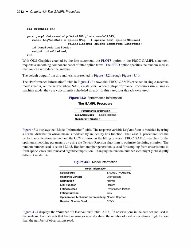
ods graphics on;
proc gampl data=sashelp.Vote1980 plots seed=12345;model LogVoteRate = spline(Pop ) spline(Edu) spline(Houses)
spline(Income) spline(Longitude Latitude);id Longitude Latitude;output out=VotePred;
run;
With ODS Graphics enabled by the first statement, the PLOTS option in the PROC GAMPL statementrequests a smoothing component panel of fitted spline terms. The SEED option specifies the random seed sothat you can reproduce the analysis.
The default output from this analysis is presented in Figure 43.2 through Figure 43.10.
The “Performance Information” table in Figure 43.2 shows that PROC GAMPL executed in single-machinemode (that is, on the server where SAS is installed). When high-performance procedures run in single-machine mode, they use concurrently scheduled threads. In this case, four threads were used.
Figure 43.2 Performance Information
The GAMPL ProcedureThe GAMPL Procedure
Performance Information
Execution Mode Single-Machine
Number of Threads 4
Figure 43.3 displays the “Model Information” table. The response variable LogVoteRate is modeled by usinga normal distribution whose mean is modeled by an identity link function. The GAMPL procedure uses theperformance iteration method and the GCV criterion as the fitting criterion. PROC GAMPL searches for theoptimum smoothing parameters by using the Newton-Raphson algorithm to optimize the fitting criterion. Therandom number seed is set to 12,345. Random number generation is used for sampling from observations toform spline knots and truncated eigendecomposition. Changing the random number seed might yield slightlydifferent model fits.
Figure 43.3 Model Information
Model Information
Data Source SASHELP.VOTE1980
Response Variable LogVoteRate
Distribution Normal
Link Function Identity
Fitting Method Performance Iteration
Fitting Criterion GCV
Optimization Technique for Smoothing Newton-Raphson
Random Number Seed 12345
Figure 43.4 displays the “Number of Observations” table. All 3,107 observations in the data set are used inthe analysis. For data sets that have missing or invalid values, the number of used observations might be lessthan the number of observations read.

Getting Started: GAMPL Procedure F 2943
Figure 43.4 Number of Observations
Number of Observations Read 3107
Number of Observations Used 3107
Figure 43.5 displays the convergence status of the performance iteration method.
Figure 43.5 Convergence Status
The performance iteration converged after 3 steps.
Figure 43.6 shows the “Fit Statistics” table. The penalized log likelihood and the roughness penalty aredisplayed. You can use effective degrees of freedom to compare generalized additive models with generalizedlinear models that do not have spline transformations. Information criteria such as Akaike’s informationcriterion (AIC), Akaike’s bias-corrected information criterion (AICC), and Schwarz Bayesian informationcriterion (BIC) can also be used for comparisons. These criteria penalize the –2 log likelihood for effectivedegrees of freedom. The GCV criterion is used to compare against other generalized additive models ormodels that are penalized.
Figure 43.6 Fit Statistics
Fit Statistics
Penalized Log Likelihood 2729.51482
Roughness Penalty 0.25787
Effective Degrees of Freedom 48.70944
Effective Degrees of Freedom for Error 3055.44725
AIC (smaller is better) -5361.86863
AICC (smaller is better) -5360.28467
BIC (smaller is better) -5067.59479
GCV (smaller is better) 0.01042
.
The “Parameter Estimates” table in Figure 43.7 shows the regression parameter and dispersion parameter esti-mates. In this model, the intercept is the only regression parameter because (1) all variables are characterizedby spline terms and no parametric effects are present and (2) the intercept absorbs the constant effect that isextracted from each spline term to make fitted splines identifiable. The dispersion parameter is estimated bymaximizing the likelihood, given other model parameters.
Figure 43.7 Regression Parameter Estimates
Parameter Estimates
Parameter DF EstimateStandard
Error Chi-Square Pr > ChiSq
Intercept 1 -0.576234 0.001803 102119.645 <.0001
Dispersion 1 0.010103 0.014287

2944 F Chapter 43: The GAMPL Procedure
The “Estimates for Smoothing Components” table is shown in Figure 43.8. For each spline term, theeffective degrees of freedom, the estimated smoothing parameter, and the corresponding roughness penaltyare displayed. The table also displays additional information about spline terms, such as the number ofparameters, penalty matrix rank, and number of spline knots.
Figure 43.8 Estimates for Smoothing Components
Estimates for Smoothing Components
ComponentEffective
DFSmoothingParameter
RoughnessPenalty
Number ofParameters
Rank ofPenalty
MatrixNumber of
Knots
Spline(Pop) 7.80559 0.0398 0.0114 9 10 2000
Spline(Edu) 7.12453 0.2729 0.0303 9 10 2000
Spline(Houses) 7.20940 0.1771 0.0370 9 10 2000
Spline(Income) 5.92854 0.7498 0.0488 9 10 2000
Spline(Longitude Latitude) 18.64138 0.000359 0.1304 19 20 2000
Figure 43.9 displays the hypothesis testing results for each smoothing component. The null hypothesis foreach spline term is whether the total dependency on each variable is 0. The effective degrees of freedom forboth fit and test is displayed.
Figure 43.9 Tests for Smoothing Components
Tests for Smoothing Components
ComponentEffective
DFEffective
DF for Test F Value Pr > F
Spline(Pop) 7.80559 8 1443.64 <.0001
Spline(Edu) 7.12453 8 153.94 <.0001
Spline(Houses) 7.20940 8 1213.94 <.0001
Spline(Income) 5.92854 7 43.17 <.0001
Spline(Longitude Latitude) 18.64138 19 1619.15 <.0001
Figure 43.10 displays the “Smoothing Component Panel” for all the spline terms used in the model. Itdisplays predicted spline curves and 95% Bayesian posterior confidence bands for each univariate splineterm.

Getting Started: GAMPL Procedure F 2945
Figure 43.10 Smoothing Component Panel
The preceding program contains an ID statement and an OUTPUT statement. The ID statement transfers thespecified variables (Longitude and Latitude) from the input data set, sashelp.Vote1980, to the output dataset, VotePred. The OUTPUT statement requests the prediction for each observation by default and saves theresults in the data set VotePred. The following run of the SGRENDER procedure produces the fitted surfaceof the log vote proportion in the 1980 presidential election:
proc sgrender data=VotePred template=surface;dynamic _title='Predicted US County Vote Proportion in the 1980 Election'
_z ='Pred';run;
Figure 43.11 shows the map of predictions of the logarithm transformation of the proportion of countypopulation who voted for any candidates in the 1980 US presidential election from the fitted generalizedadditive model.

2946 F Chapter 43: The GAMPL Procedure
Figure 43.11 Predicted US County Vote Proportion in the 1980 Election
Compared to the map of the logarithm transformations of the proportion of votes cast shown in Figure 43.1,the map of the predictions of the logarithm transformations of the proportion of votes cast has a smoothersurface.
Syntax: GAMPL Procedure F 2947
Syntax: GAMPL ProcedureThe following statements are available in the GAMPL procedure:
PROC GAMPL < options > ;CLASS variable < (options) >: : : < variable < (options) > > < / global-options > ;MODEL response < (response-options) > = < PARAM(effects) >
< spline-effects > < / model-options > ;MODEL events / trials = < PARAM(effects) > < spline-effects > < / model-options > ;OUTPUT < OUT=SAS-data-set > < keyword < =name > >. . . < keyword < =name > > < / options > ;PERFORMANCE performance-options ;FREQ variable ;ID variables ;WEIGHT variable ;
The PROC GAMPL statement and at least one MODEL statement are required. The CLASS statementcan appear multiple times. If a CLASS statement is specified, it must precede the MODEL statements.The following sections describe the PROC GAMPL statement and then describe the other statements inalphabetical order.
PROC GAMPL StatementPROC GAMPL < options > ;
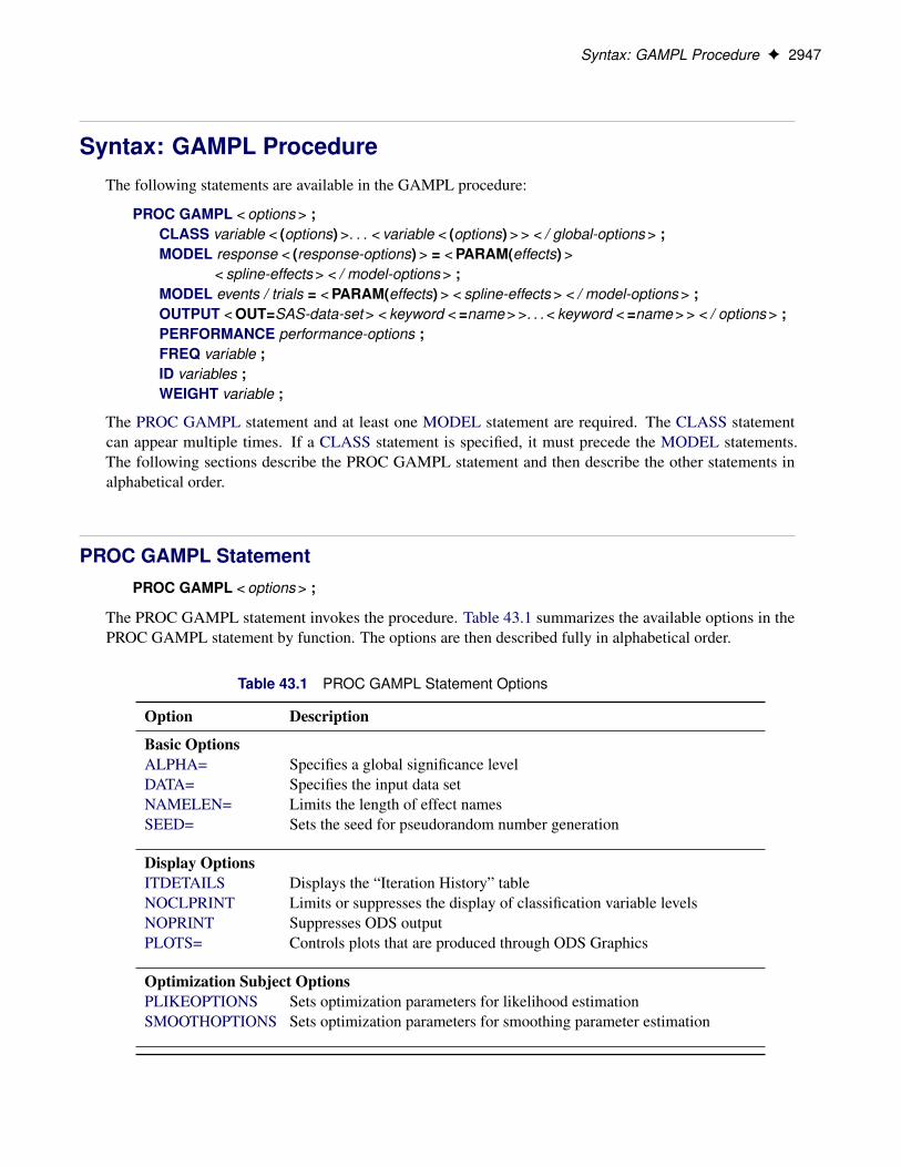
The PROC GAMPL statement invokes the procedure. Table 43.1 summarizes the available options in thePROC GAMPL statement by function. The options are then described fully in alphabetical order.
Table 43.1 PROC GAMPL Statement Options
Option Description
Basic OptionsALPHA= Specifies a global significance levelDATA= Specifies the input data setNAMELEN= Limits the length of effect namesSEED= Sets the seed for pseudorandom number generation
Display OptionsITDETAILS Displays the “Iteration History” tableNOCLPRINT Limits or suppresses the display of classification variable levelsNOPRINT Suppresses ODS outputPLOTS= Controls plots that are produced through ODS Graphics
Optimization Subject OptionsPLIKEOPTIONS Sets optimization parameters for likelihood estimationSMOOTHOPTIONS Sets optimization parameters for smoothing parameter estimation
2948 F Chapter 43: The GAMPL Procedure
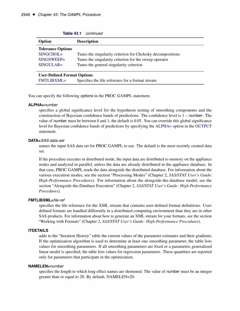
Table 43.1 continued
Option Description
Tolerance OptionsSINGCHOL= Tunes the singularity criterion for Cholesky decompositionsSINGSWEEP= Tunes the singularity criterion for the sweep operatorSINGULAR= Tunes the general singularity criterion
User-Defined Format OptionsFMTLIBXML= Specifies the file reference for a format stream
You can specify the following options in the PROC GAMPL statement.
ALPHA=numberspecifies a global significance level for the hypothesis testing of smoothing components and theconstruction of Bayesian confidence bands of predictions. The confidence level is 1 – number . Thevalue of number must be between 0 and 1; the default is 0.05. You can override this global significancelevel for Bayesian confidence bands of predictions by specifying the ALPHA= option in the OUTPUTstatement.
DATA=SAS-data-setnames the input SAS data set for PROC GAMPL to use. The default is the most recently created dataset.
If the procedure executes in distributed mode, the input data are distributed to memory on the appliancenodes and analyzed in parallel, unless the data are already distributed in the appliance database. Inthat case, PROC GAMPL reads the data alongside the distributed database. For information about thevarious execution modes, see the section “Processing Modes” (Chapter 2, SAS/STAT User’s Guide:High-Performance Procedures). For information about the alongside-the-database model, see thesection “Alongside-the-Database Execution” (Chapter 2, SAS/STAT User’s Guide: High-PerformanceProcedures).
FMTLIBXML=file-refspecifies the file reference for the XML stream that contains user-defined format definitions. User-defined formats are handled differently in a distributed computing environment than they are in otherSAS products. For information about how to generate an XML stream for your formats, see the section“Working with Formats” (Chapter 2, SAS/STAT User’s Guide: High-Performance Procedures).
ITDETAILSadds to the “Iteration History” table the current values of the parameter estimates and their gradients.If the optimization algorithm is used to determine at least one smoothing parameter, the table listsvalues for smoothing parameters. If all smoothing parameters are fixed or a parametric generalizedlinear model is specified, the table lists values for regression parameters. These quantities are reportedonly for parameters that participate in the optimization.
NAMELEN=numberspecifies the length to which long effect names are shortened. The value of number must be an integergreater than or equal to 20. By default, NAMELEN=20.

PROC GAMPL Statement F 2949
NOCLPRINT< =number >suppresses the display of the “Class Level Information” table if you do not specify number . If youspecify number , the values of the classification variables are displayed for only those variables whosenumber of levels is less than number . Specifying a number helps reduce the size of the “Class LevelInformation” table if some classification variables have a large number of levels.
NOPRINTsuppresses the generation of ODS output.
PLIKEOPTIONS(optimization-parameters)sets optimization parameters for either maximum or penalized likelihood estimation. For moreinformation about how to specify optimization-parameters, see the section “Optimization Parameters”on page 2950.
PLOTS < (global-plot-option) > < = plot-requests < (option) > >controls the plots that are produced through ODS Graphics. When ODS Graphics is enabled, PROCGAMPL produces by default a panel of plots of partial prediction curves or surfaces of smoothingcomponents.
ODS Graphics must be enabled before plots can be requested. For example:
ods graphics on;
proc gampl plots;model y=spline(x1) spline(x2);
run;
ods graphics off;
For more information about enabling and disabling ODS Graphics, see the section “Enabling andDisabling ODS Graphics” on page 607 in Chapter 21, “Statistical Graphics Using ODS.”
You can specify the following global-plot-option, which applies to the smoothing component plots thatthe GAMPL procedure generates:
UNPACK | UNPACKPANELsuppresses paneling. By default, multiple smoothing component plots can appear in some outputpanels. Specify UNPACK to get each plot individually.
You can specify the following plot-requests:
ALLrequests that all default plots be produced.
COMPONENTS < (component-option) >plots a panel of smoothing components of the fitted model. You can specify the followingcomponent-option:
COMMONAXESrequests that the smoothing component plots use a common vertical axis except for bivariatecontour plots. This option enables you to visually judge the relative effect size.

2950 F Chapter 43: The GAMPL Procedure
NONEsuppresses all plots.
SEED=numberspecifies an integer that is used to start the pseudorandom number generator for subset sampling fromobservations to form knots if necessary and for truncated eigendecomposition. If you do not specifythis option, or if number � 0, the seed is generated from the time of day, which is read from thecomputer’s clock.
SINGCHOL=numbertunes the singularity criterion in Cholesky decompositions. The default is 1E4 times the machineepsilon; this product is approximately 1E–12 on most computers.
SINGSWEEP=numbertunes the singularity criterion in sweep operations that determine collinearity between spline basisexpansions. The default is 1E–8.
SINGULAR=numbertunes the general singularity criterion that is applied in sweep and inversion operations. The default is1E4 times the machine epsilon; this product is approximately 1E–12 on most computers.
SMOOTHOPTIONS(optimization-parameters)specifies optimization parameters for smoothing parameter estimation. For more information abouthow to specify optimization-parameters, see the section “Optimization Parameters” on page 2950.
Optimization Parameters
You can specify optimization-parameters for both the PLIKEOPTIONS and SMOOTHOPTIONS options.Depending on the modeling context, some optimization parameters might have no effect. For parametric gen-eralized linear models or generalized additive models that have fixed smoothing parameters, any optimizationparameters that you specify in the SMOOTHOPTIONS option are ignored. For the performance iterationmethod, only the ABSFCONV=, FCONV=, and MAXITER= options are effective for PLIKEOPTIONS.The optimization algorithm is considered to have converged when any one of the convergence criteria thatare specified in optimization-parameters is satisfied. Table 43.2 lists the available optimization parametersfor both the PLIKEOPTIONS and SMOOTHOPTIONS options.
Table 43.2 Optimization Parameters
Option Description
ABSCONV= Tunes the absolute function convergence criterionABSFCONV= Tunes the absolute function difference convergence criterionABSGCONV= Tunes the absolute gradient convergence criterionFCONV= Tunes the relative function difference convergence criterionGCONV= Tunes the relative gradient convergence criterionMAXFUNC= Specifies the maximum number of function evaluations in any optimizationMAXITER= Chooses the maximum number of iterations in any optimizationMAXTIME= Specifies the upper limit of CPU time (in seconds) for any optimizationMINITER= Specifies the minimum number of iterations in any optimizationTECHNIQUE= Selects the optimization technique

PROC GAMPL Statement F 2951
You can specify the following optimization-parameters:
ABSCONV=r
ABSTOL=rspecifies an absolute function convergence criterion. For minimization, termination requires f . .k// �r , where is the vector of parameters in the optimization and f .�/ is the objective function. Thedefault value of r is the negative square root of the largest double-precision value, which serves only asa protection against overflow.
ABSFCONV=r < n >
ABSFTOL=r < n >specifies an absolute function difference convergence criterion. For all techniques except NMSIMP,termination requires a small change of the function value in successive iterations,
jf . .k�1// � f . .k//j � r
where denotes the vector of parameters that participate in the optimization and f .�/ is the objectivefunction. The same formula is used for the NMSIMP technique, but .k/ is defined as the vertex thathas the lowest function value and .k�1/ is defined as the vertex that has the highest function value inthe simplex. The optional integer value n specifies the number of successive iterations for which thecriterion must be satisfied before the process terminates. By default, ABSFCONV=0.
ABSGCONV=r < n >
ABSGTOL=r < n >specifies an absolute gradient convergence criterion. Termination requires the maximum absolutegradient element to be small,
maxjjgj .
.k//j � r
where denotes the vector of parameters that participate in the optimization and gj .�/ is the gradientof the objective function with respect to the jth parameter. This criterion is not used by the NMSIMPtechnique. The default value is r = 1E–8. The optional integer value n specifies the number ofsuccessive iterations for which the criterion must be satisfied before the process terminates.
FCONV=r < n >
FTOL=r < n >specifies a relative function difference convergence criterion. For all techniques except NMSIMP,termination requires a small relative change of the function value in successive iterations,
jf . .k// � f . .k�1//j
jf . .k�1//j� r
where denotes the vector of parameters that participate in the optimization and f .�/ is the objectivefunction. The same formula is used for the NMSIMP technique, but .k/ is defined as the vertex thathas the lowest function value and .k�1/ is defined as the vertex that has the highest function value inthe simplex.
The default value is r = 2��, where � is the machine precision. The optional integer value n specifies thenumber of successive iterations for which the criterion must be satisfied before the process terminates.

2952 F Chapter 43: The GAMPL Procedure
GCONV=r < n >
GTOL=r < n >specifies a relative gradient convergence criterion. For all techniques except CONGRA and NMSIMP,termination requires that the normalized predicted function reduction be small,
g. .k//0ŒH.k/��1g. .k//jf . .k//j
� r
where denotes the vector of parameters that participate in the optimization, f .�/ is the objectivefunction, and g.�/ is the gradient. For the CONGRA technique (where a reliable Hessian estimate, H,is not available), the following criterion is used:
k g. .k// k22 k s. .k// k2k g. .k// � g. .k�1// k2 jf . .k//j
� r
This criterion is not used by the NMSIMP technique. The default value is r = 1E–8. The optionalinteger value n specifies the number of successive iterations for which the criterion must be satisfiedbefore the process terminates.
MAXFUNC=n
MAXFU=nspecifies the maximum number of function calls in the optimization process. The default values are asfollows, depending on the optimization technique that you specify in the TECHNIQUE= option:
� TRUREG, NRRIDG, NEWRAP: n = 125
� QUANEW, DBLDOG: n = 500
� CONGRA: n = 1,000
� NMSIMP: n = 3,000
The optimization can terminate only after completing a full iteration. Therefore, the number of functioncalls that are actually performed can exceed n.
MAXITER=n
MAXIT=nspecifies the maximum number of iterations in the optimization process. The default values are asfollows, depending on the optimization technique that you specify in the TECHNIQUE option:
� TRUREG, NRRIDG, NEWRAP: n = 50
� QUANEW, DBLDOG: n = 200
� CONGRA: n = 400
� NMSIMP: n = 1,000
These default values also apply when n is specified as a missing value.

CLASS Statement F 2953
MAXTIME=rspecifies an upper limit of r seconds of CPU time for the optimization process. The default value is thelargest floating-point double representation of your computer. The time that you specify in this optionis checked only once at the end of each iteration. Therefore, the actual running time can be longer thanr .
MINITER=n
MINIT=nspecifies the minimum number of iterations. If you request more iterations than are actually needed forconvergence to a stationary point, the optimization algorithms might behave strangely. For example,the effect of rounding errors can prevent the algorithm from continuing for the required number ofiterations. By default, MINITER=0.
TECHNIQUE=keyword
TECH=keywordspecifies the optimization technique for obtaining smoothing parameter estimates and regressionparameter estimates. You can choose from the following techniques:
CONGRA performs a conjugate-gradient optimization.
DBLDOG performs a version of double-dogleg optimization.
NEWRAP performs a Newton-Raphson optimization with line search.
NMSIMP performs a Nelder-Mead simplex optimization.
NONE performs no optimization.
NRRIDG performs a Newton-Raphson optimization with ridging.
QUANEW performs a dual quasi-Newton optimization.
TRUREG performs a trust-region optimization
By default, TECHNIQUE=NEWRAP for the performance iteration (METHOD=PERFORMANCE),and TECHNIQUE=QUANEW for the outer iteration (METHOD=OUTER).
For more information, see the section “Choosing an Optimization Technique” on page 2975.
CLASS StatementCLASS variable < (options) >: : : < variable < (options) > > < / global-options > ;
The CLASS statement names the classification variables to be used as explanatory variables in the analysis.The CLASS statement must precede the MODEL statement. You can list the response variable for binarymodels in the CLASS statement, but this is not necessary.
The CLASS statement is documented in the section “CLASS Statement” (Chapter 3, SAS/STAT User’s Guide:High-Performance Procedures).

2954 F Chapter 43: The GAMPL Procedure
FREQ StatementFREQ variable ;
The variable in the FREQ statement identifies a numeric variable in the data set that contains the frequencyof occurrence of each observation. PROC GAMPL treats each observation as if it appeared f times, wherethe frequency value f is the value of the FREQ variable for the observation. If f is not an integer, then f istruncated to an integer. If f is less than 1 or missing, the observation is not used in the analysis. When you donot specify the FREQ statement, each observation is assigned a frequency of 1.
ID StatementID variables ;
The ID statement lists one or more variables from the input data set that are to be transferred to the outputdata set that you specify in the OUTPUT statement.
For more information, see the section “ID Statement” (Chapter 3, SAS/STAT User’s Guide: High-PerformanceProcedures).
MODEL StatementMODEL response < (response-options) > = < PARAM(effects) > < spline-effects > < / model-options > ;
MODEL events / trials = < PARAM(effects) > < spline-effects > < / model-options > ;
The MODEL statement specifies the response (dependent or target) variable and the predictor (independentor explanatory) effects of the model. You can specify the response in the form of a single variable or in theform of a ratio of two variables, which are denoted events/trials. The first form applies to all distributionfamilies; the second form applies only to summarized binomial response data. When you have binomial data,the events variable contains the number of positive responses (or events) and the trials variable contains thenumber of trials. The values of both events and (trials – events) must be nonnegative, and the value of trialsmust be positive. If you specify a single response variable that is in a CLASS statement, then the response isassumed to be binary.
You can specify parametric effects that are constructed from variables in the input data set and includethe effects in the parentheses of a PARAM( ) option, which can appear multiple times. For informationabout constructing the model effects, see the section “Specification and Parameterization of Model Effects”(Chapter 3, SAS/STAT User’s Guide: High-Performance Procedures).
You can specify spline-effects by including independent variables inside the parentheses of the SPLINE( )option. Only continuous variables (not classification variables) can be specified in spline-effects. Eachspline-effect can have at least one variable and optionally some spline-options. You can specify any numberof spline-effects. The following table shows some examples.

MODEL Statement F 2955
Spline Effect Specification Meaning
Spline(x) Constructs the univariate spline with x and usesthe observed data points as knots. The maximumdegrees of freedom is 10. PROC GAMPL uses anoptimization algorithm to determine the optimalsmoothing parameter.
Spline(x1/knots=list(1 to 10)) Constructs the univariate spline by using x1 and asupplied list of knots from 1 to 10. PROC GAMPLuses an optimization algorithm to determine theoptimal smoothing parameter.
Spline(x2 x3/smooth=0.3) Constructs the bivariate spline by using x2 and x3and a fixed smoothing parameter 0.3.
Spline(x4 x5 x6/maxdf=40) Constructs the trivariate spline by using x4, x5,and x6 and a maximum of 40 degrees of freedom.PROC GAMPL uses an optimization algorithm todetermine the optimal smoothing parameter.
Both parametric effects and spline effects are optional. If none are specified, a model that contains only anintercept is fitted. If only parametric effects are present, PROC GAMPL fits a parametric generalized linearmodel by using the terms inside the parentheses of all PARAM( ) terms. If only spline effects are present,PROC GAMPL fits a nonparametric additive model. If both types of effects are present, PROC GAMPL fitsa semiparametric model by using the parametric effects as the linear part of the model.
There are three sets of options in the MODEL statement. The response-options determine how the GAMPLprocedure models probabilities for binary data. The spline-options controls how each spline term formsbasis expansions. The model-options control other aspects of model formation and inference. Table 43.3summarizes these options.
Table 43.3 MODEL Statement Options
Option Description
Response Variable Options for Binary ModelsDESCENDING Reverses the response categoriesEVENT= Specifies the event categoryORDER= Specifies the sort orderREF= Specifies the reference category
Smoothing Options for Spline EffectsDETAILS Requests detailed spline informationDF= Specifies the fixed degrees of freedomINITSMOOTH= Specifies the starting value for the smoothing parameterKNOTS= Specifies the knots to be used for constructing the splineM= Specifies polynomial orders for constructing the splineMAXDF= Specifies the maximum degrees of freedomMAXKNOTS= Specifies the maximum number of knots to be used for constructing the splineMAXSMOOTH= Specifies the upper bound for the smoothing parameter

2956 F Chapter 43: The GAMPL Procedure
Table 43.3 continued
Option Description
MINSMOOTH= Specifies the lower bound for the smoothing parameterSMOOTH= Specifies a fixed smoothing parameter
Model OptionsALLOBS Requests all nonmissing values of spline variables for constructing spline
basis functions regardless of other model variablesCRITERION= Specifies the model evaluation criterionDISPERSION | PHI= Specifies the fixed dispersion parameterDISTRIBUTION | DIST= Specifies the response distributionFDHESSIAN Requests a finite-difference Hessian for smoothing parameter selectionINITIALPHI= Specifies the starting value of the dispersion parameterLINK= Specifies the link functionNORMALIZE Requests normalized spline basis functions for model fittingMAXPHI= Specifies the upper bound for searching the dispersion parameterMETHOD= Specifies the algorithm for selecting smoothing parametersMINPHI= Specifies the lower bound for searching the dispersion parameterOFFSET= Specifies the offset variableRIDGE= Specifies the ridge parameterSCALE= Specifies the method for estimating the dispersion parameter
Response Variable Options
Response variable options determine how the GAMPL procedure models probabilities for binary data.
You can specify the following response-options by enclosing them in parentheses after the response variable.
DESCENDING
DESCreverses the order of the response categories. If you specify both the DESCENDING and ORDER=options, PROC GAMPL orders the response categories according to the ORDER= option and thenreverses that order.
EVENT=‘category ’ | FIRST | LASTspecifies the event category for the binary response model. PROC GAMPL models the probabilityof the event category. The EVENT= option has no effect when there are more than two responsecategories.
You can specify any of the following:
‘category ’specifies that observations whose value matches category (formatted, if a format is applied) inquotation marks represent events in the data. For example, the following statements specify thatobservations that have a formatted value of ‘1’ represent events in the data. The probability thatis modeled by the GAMPL procedure is thus the probability that the variable def takes on the(formatted) value ‘1’.
MODEL Statement F 2957
proc gampl data=MyData;class A B C;model def(event ='1') = param(A B C) spline(x1 x2 x3);
run;
FIRSTdesignates the first ordered category as the event.
LASTdesignates the last ordered category as the event.
By default, EVENT=FIRST.
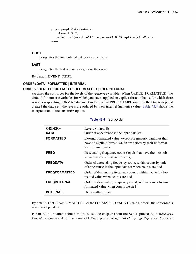
ORDER=DATA | FORMATTED | INTERNAL
ORDER=FREQ | FREQDATA | FREQFORMATTED | FREQINTERNALspecifies the sort order for the levels of the response variable. When ORDER=FORMATTED (thedefault) for numeric variables for which you have supplied no explicit format (that is, for which thereis no corresponding FORMAT statement in the current PROC GAMPL run or in the DATA step thatcreated the data set), the levels are ordered by their internal (numeric) value. Table 43.4 shows theinterpretation of the ORDER= option.
Table 43.4 Sort Order
ORDER= Levels Sorted ByDATA Order of appearance in the input data set
FORMATTED External formatted value, except for numeric variables thathave no explicit format, which are sorted by their unformat-ted (internal) value
FREQ Descending frequency count (levels that have the most ob-servations come first in the order)
FREQDATA Order of descending frequency count; within counts by orderof appearance in the input data set when counts are tied
FREQFORMATTED Order of descending frequency count; within counts by for-matted value when counts are tied
FREQINTERNAL Order of descending frequency count; within counts by un-formatted value when counts are tied
INTERNAL Unformatted value
By default, ORDER=FORMATTED. For the FORMATTED and INTERNAL orders, the sort order ismachine-dependent.
For more information about sort order, see the chapter about the SORT procedure in Base SASProcedures Guide and the discussion of BY-group processing in SAS Language Reference: Concepts.

2958 F Chapter 43: The GAMPL Procedure
REF=‘category ’ | FIRST | LASTspecifies the reference category for the binary response model. Specifying one response category asthe reference is the same as specifying the other response category as the event category. You canspecify any of the following:
‘category ’specifies that observations whose value matches category (formatted, if a format is applied) aredesignated as the reference.
FIRSTdesignates the first ordered category as the reference
LASTdesignates the last ordered category as the reference.
By default, REF=LAST.
Spline Options
DETAILSrequests a detailed spline specification information table.
DF=numberspecifies a fixed degrees of freedom. When you specify this option, no smoothing parameter selectionis performed on the spline term. If number is not an integer, then number is truncated to an integer.
INITSMOOTH=numberspecifies the starting value for a smoothing parameter. The number must be nonnegative.
KNOTS=methodspecifies the method for supplying user-defined knot values instead of using data values for constructingbasis expansions. You can use the following methods for supplying the knots:
LIST(list-of-values)specifies a list of values as knots for the spline construction. For a multivariate spline term, thelisted values are taken as multiple row vectors, where each vector has values that are orderedby specified variables. If the last row vector of knots contains fewer values than the number ofvariables, then the last row vector is ignored. For example, the following specification of a splineterm produces two actual knot vectors (k1 and k2) and the value 5 is ignored.
spline(x1 x2/knots=list(1 2 3 4 5))
Table 43.5 Knot Values for a Bivariate Spline with a Supplied List
x1 x2k1 1 2k2 3 4

MODEL Statement F 2959
EQUAL(n)specifies the number of equally spaced interior knots for every variable in a spline term. Twoboundary knots are automatically added to the knot list for each variable such that the totalnumber of knots is .n C 2/d , where d is the number of variables in the spline term. For amultivariate spline term, knot values for each variable are determined independently from thecorresponding boundary values. For example, if the boundary points for x1 are 1 and 5 and theboundary points for x2 are 2 and 6, then the following specification of a spline term producesnine actual knots (k1 — k9), which consist of two boundary knots and one interior knot for eachvariable.
spline(x1 x2/knots=equal(1))
Table 43.6 Knot Values for a Bivariate Spline with One Interior Knot
x1 x2k1 1 2k2 1 4k3 1 6k4 3 2k5 3 4k6 3 6k7 5 2k8 5 4k9 5 6
M=numberspecifies the order of the derivative in the penalty term. The number must be a positive integer. Thedefault is max.2; int.d=2/C 1/, where d is the number of variables in the spline term.
MAXDF=numberspecifies the maximum number of degrees of freedom. When a thin-plate regression spline is formed,the specified number is used for constructing a low-rank penalty matrix to approximate the penaltymatrix via the truncated eigendecomposition. The number must be greater than
�mCd�1d
�, where m is
the derivative order that is specified in the M= option. The default is 10 � d . For more information,see the section “Thin-Plate Regression Splines” on page 2965.
MAXKNOTS=numberspecifies the maximum number of knots if data points are used to form knots. If KNOTS=LIST(list-of-values) is not specified, PROC GAMPL forms knots from unique data points. If the number ofunique data points is greater than number , a subset of size number is formed by random samplingfrom all unique data points. The number cannot exceed the largest integer that can be stored on thegiven machine. By default, MAXKNOTS=2000.
MAXSMOOTH=numberspecifies the upper bound for the smoothing parameter. The default is the largest double-precisionvalue.

2960 F Chapter 43: The GAMPL Procedure
MINSMOOTH=numberspecifies the lower bound for the smoothing parameter. By default, MINSMOOTH=0.
SMOOTH=numberspecifies a fixed smoothing parameter. When you specify this option, no smoothing parameter selectionis performed on the spline term.
Model Options
ALLOBSrequests that all nonmissing values of the variables be specified in a spline term for constructing thespline basis functions, regardless of whether other model variables are missing.
CRITERION=criterionspecifies the model evaluation criterion for selecting smoothing parameters for spline-effects. You canspecify the following values:
GACV< (FACTOR=number | GAMMA=number ) >uses the generalized approximate cross validation (GACV) criterion to evaluate models.
GCV< (FACTOR=number | GAMMA=number ) >uses the generalized cross validation (GCV) criterion to evaluate models.
UBRE< (FACTOR=number | GAMMA=number ) >uses the unbiased risk estimator (UBRE) criterion to evaluate models.
The default criterion depends on the value of the DISTRIBUTION= option. For distributions thatinvolve dispersion parameters, GCV is the default. For distributions without dispersion parameters,UBRE is the default. For all three criteria, you can optionally use the FACTOR= option to specify anextra tuning parameter in order to penalize more for model roughness. The value of number mustbe greater than or equal to 1. For more information about the model evaluation criteria, see “ModelEvaluation Criteria” on page 2969.
DISPERSION=numberspecifies a fixed dispersion parameter for distributions that have a dispersion parameter. The dispersionparameter that is used in all computations is fixed at number ; it is not estimated.
DISTRIBUTION=keywordspecifies the response distribution for the model. The keywords and their associated distributions areshown in Table 43.7.

MODEL Statement F 2961
Table 43.7 Built-In Distribution Functions
DistributionDISTRIBUTION= Function
BINARY BinaryBINOMIAL Binary or binomialGAMMA GammaINVERSEGAUSSIAN | IG Inverse GaussianNEGATIVEBINOMIAL | NB Negative binomialNORMAL | GAUSSIAN NormalPOISSON Poisson
If you do not specify a link function in the LINK= option, a default link function is used. The defaultlink function for each distribution is shown in Table 43.8. You can use any link function shown inTable 43.9 by specifying the LINK= option. Other commonly used link functions for each distributionare shown in Table 43.8.
Table 43.8 Default and Commonly Used Link Functions
Default Other Commonly UsedDISTRIBUTION= Link Function Link Functions
BINARY Logit Probit, complementary log-log, log-logBINOMIAL Logit Probit, complementary log-log, log-logGAMMA Reciprocal LogINVERSEGAUSSIAN | IG Reciprocal square LogNEGATIVEBINOMIAL | NB LogNORMAL | GAUSSIAN Identity LogPOISSON Log
FDHESSIANrequests that the second-order derivatives (Hessian) be computed using finite-difference approximationsbased on evaluation of the first-order derivatives (gradient). This option might be useful if the analyticalHessian takes a long time to compute.
INITIALPHI=numberspecifies a starting value for iterative maximum likelihood estimation of the dispersion parameter fordistributions that have a dispersion parameter.
LINK=keywordspecifies the link function for the model. The keywords and the associated link functions are shownin Table 43.9. Default and commonly used link functions for the available distributions are shown inTable 43.8.

2962 F Chapter 43: The GAMPL Procedure
Table 43.9 Built-In Link Functions
LinkLINK= Function g.�/ D � D
CLOGLOG | CLL Complementary log-log log.� log.1 � �//IDENTITY | ID Identity �
INV | RECIP Reciprocal 1=�
INV2 Reciprocal square 1=�2
LOG Logarithm log.�/LOGIT Logit log.�=.1 � �//LOGLOG Log-log � log.� log.�//PROBIT Probit ˆ�1.�/
ˆ�1.�/ denotes the quantile function of the standard normal distribution.
MAXPHI=numberspecifies an upper bound for maximum likelihood estimation of the dispersion parameter for distribu-tions that have a dispersion parameter.
METHOD=OUTER | PERFORMANCEspecifies the algorithm for selecting smoothing parameters for spline-effects. You can specify thefollowing values:
OUTER specifies the outer iteration method for selecting smoothing parameters. For moreinformation about the method, see the section “Outer Iteration (Experimental)” onpage 2971.
NOTE: The outer iteration method is experimental in this release.
PERFORMANCE specifies the performance iteration method for selecting smoothing parameters.For more information about the method, see the section “Performance Iteration” onpage 2971.
By default, METHOD=PERFORMANCE.
MINPHI=numberspecifies a lower bound for maximum likelihood estimation of the dispersion parameter for distributionsthat have a dispersion parameter.
NORMALIZErequests normalized spline basis functions for model fitting. After the regression spline basis functionsare computed, each column is standardized to have a unit standard error. The corresponding penaltymatrix is also scaled accordingly. This option might be helpful when you have badly scaled data.
OFFSET=variablespecifies a variable to be used as an offset to the linear predictor. An offset plays the role of an effectwhose coefficient is known to be 1. The offset variable cannot appear in the CLASS statement orelsewhere in the MODEL statement. Observations that have missing values for the offset variable areexcluded from the analysis.
OUTPUT Statement F 2963
RIDGE=numberallows a ridge parameter such that a diagonal matrix H W Hi i D number is added to the optimizationproblem with respect to regression parameters:
min.y � Xˇ/0.y � Xˇ/C ˇ0S�ˇ C ˇ0Hˇ with respect to ˇ
By default, RIDGE=0. Specifying a small ridge parameter might be helpful if the model matrixX0XC S� is close to singular.
SCALE=DEVIANCE | MLE | PEARSONspecifies the method for estimating the scale and dispersion parameters. You can specify the followingvalues:
DEVIANCEestimates the dispersion parameter by using the deviance statistic.
MLEcomputes the dispersion parameter by maximizing the likelihood or penalized likelihood.
PEARSONestimates the dispersion parameter by using Pearson’s statistic.
By default, SCALE=MLE.
OUTPUT StatementOUTPUT < OUT=SAS-data-set >
< keyword < =name > >. . . < keyword < =name > > < / options > ;
The OUTPUT statement creates a data set that contains observationwise statistics that are computed after themodel is fitted. The variables in the input data set are not included in the output data set in order to avoid dataduplication for large data sets; however, variables that are specified in the ID statement are included.
If the input data set is distributed (so that accessing data in a particular order cannot be guaranteed), theGAMPL procedure copies the distribution or partition key to the output data set so that its contents can bejoined with the input data.
The computation of the output statistics is based on the final parameter estimates. If the model fit does notconverge, missing values are produced for the quantities that depend on the estimates.
You can specify the following syntax elements in the OUTPUT statement before the slash (/).
OUT=SAS-data-set
DATA=SAS-data-setspecifies the name of the output data set. If you omit this option, PROC GAMPL uses the DATAnconvention to name the output data set.
keyword < =name >specifies a statistic to include in the output data set and optionally assigns a name to the variable. Ifyou do not provide a name, the GAMPL procedure assigns a default name based on the keyword .
You can specify the following keywords for adding statistics to the OUTPUT data set:

2964 F Chapter 43: The GAMPL Procedure
LINP | XBETArequests the linear predictor � D x0ˇ. For observations in which only the response variable ismissing, values of the linear predictor are computed even though these observations do not affectthe model fit. The default name is Xbeta.
LOWERrequests a lower Bayesian confidence band value for the predicted value. The default name isLower.
PEARSON | PEARS | RESCHIrequests the Pearson residual, .y��/=
pV.�/, where � is the estimate of the predicted response
mean and V.�/ is the response distribution variance function. The default name is Pearson.
PREDICTED | PRED | Prequests predicted values for the response variable. For observations in which only the responsevariable is missing, the predicted values are computed even though these observations do notaffect the model fit. The default name is Pred.
RESIDUAL | RESID | Rrequests the raw residual, y � �, where � is the estimate of the predicted mean. The defaultname is Residual.
STDrequests a standard error for the linear predictor. The default name is Std.
UPPERrequests an upper Bayesian confidence band value for the predicted value. The default name isUpper.
You can specify the following options in the OUTPUT statement after the slash (/):
ALPHA=numberspecifies the significance level for the construction of Bayesian confidence bands in the OUTPUT dataset. The confidence level is 1 � number .
COMPONENTrequests componentwise statistics for all spline terms if LINP, LOWER, STD, or UPPER is specifiedas a keyword .
PERFORMANCE StatementPERFORMANCE < performance-options > ;
You can use the PERFORMANCE statement to control whether the procedure executes in single-machine ordistributed mode. The default is single-machine mode.
You can also use this statement to define performance parameters for multithreaded and distributed computing,and you can request details about performance results.
The PERFORMANCE statement is documented in the section “PERFORMANCE Statement” (Chapter 2,SAS/STAT User’s Guide: High-Performance Procedures).
WEIGHT Statement F 2965
WEIGHT StatementWEIGHT variable ;
The variable in the WEIGHT statement is used as a weight to perform a weighted analysis of the data.Observations that have nonpositive or missing weights are not included in the analysis. If a WEIGHTstatement is not included, then all observations that are used in the analysis are assigned a weight of 1.
Details: GAMPL Procedure
Missing ValuesAny observation that has missing values for the response, frequency, weight, offset, or explanatory variablesis excluded from the analysis; however, missing values are valid for response and explanatory variables ifyou specify the MISSING option in the CLASS statement. Observations that have a nonpositive weight or afrequency less than 1 are also excluded. For Poisson and negative binomial distributions, observations thathave a negative response value are excluded. For gamma and inverse Gaussian distributions, observationsthat have a nonpositive response value are excluded.
The estimated linear predictor and the fitted means are not computed for any observation that has missingoffset or explanatory variable values. However, if only the response value is missing, the linear predictor andthe fitted means can be computed and output to a data set by using the OUTPUT statement.
Thin-Plate Regression SplinesThe GAMPL procedure uses thin-plate regression splines (Wood 2003) to construct spline basis expansions.The thin-plate regression splines are based on thin-plate smoothing splines (Duchon 1976, 1977). Comparedto thin-plate smoothing splines, thin-plate regression splines produce fewer basis expansions and thus makedirect fitting of generalized additive models possible.
Thin-Plate Smoothing Splines
Consider the problem of estimating a smoothing function f of x with d covariates from n observations. Themodel assumes
yi D f .xi /C �i ; i D 1; : : : ; n
Then the thin-plate smoothing splines estimate the smoothing function f by minimizing the penalized leastsquares function:
nXiD1
.yi � f .xi //2 C �Jm;d .f /

2966 F Chapter 43: The GAMPL Procedure
The penalty term �Jm;d .f / includes the function that measures roughness on the f estimate:
Jm;d .f / D
Z� � �
Z X˛1C���C˛dDm
mŠ
˛1Š � � �˛d Š
�@mf
@x1˛1 ���@xd
˛d
�2dx1 � � � dxd
The parameter m (which corresponds to the M= option for a spline effect) specifies how the penalty is appliedto the function roughness. Function derivatives whose order is less than m are not penalized. The relation2m > d must be satisfied.
The penalty term also includes the smoothing parameter � 2 Œ0;1/, which controls the trade-off between themodel’s fidelity to the data and the function smoothness of f. When � D 0, the function estimate correspondsto an interpolation. When �!1, the function estimate becomes the least squares fit. By using the definedpenalized least squares criterion and a fixed � value, you can explicitly express the estimate of the smoothfunction f in the following form:
f�.x/ DMXjD1
�j�j .x/CnXi
ıi�m;d .kx � xik/
In the expression of f�.x/, ıi and �j are coefficients to be estimated. The functions �j .x/ correspondto unpenalized polynomials of x with degrees up to m � 1. The total number of these polynomials isM D
�mCd�1d
�. The function �m;d models the extra nonlinearity besides the polynomials and is a function
of the Euclidean distance r between any x value and an observed xi value:
�m;d .r/ D
8<:
.�1/mC1Cd=2
22m�1�d=2.m�1/Š.m�d=2/Šr2m�d log.r/ if d is even
�.d=2�m/
22m�d=2.m�1/Šr2m�d if d is odd
Define the penalty matrix E such that each entry Eij D �m;d .kxi � xj k/, let y be the vector of the response,let T be the matrix where each row is formed by �j .x/, and let � and ı be vectors of coefficients �j and ıi .Then you can obtain the function estimate f� from the following minimization problem:
min ky � T� � Eık2 C �ı0Eı subject to T0ı D 0
For more information about thin-plate smoothing splines, see Chapter 118, “The TPSPLINE Procedure.”
Low-Rank Approximation
Given the representation of the thin-plate smoothing spline, the estimate of f involves as many parameters asthe number of unique data points. Solving .�; ı/ with an optimum � becomes difficult for large problems.
Because the matrix E is symmetric and nonnegative definite, the eigendecomposition can be taken asE D UDU0, where D is the diagonal matrix of eigenvalues di of E, and U is the matrix of eigenvectors thatcorresponds to di . The truncated eigendecomposition forms QEk , which is an approximation to E such that
QEk D UkDkU0k
where Dk is a diagonal matrix that contains the k most extreme eigenvalues in descending order of absolutevalues: j Qd1j > � � � > j Qdkj. Uk is the matrix that is formed by columns of eigenvectors that correspond to theeigenvalues in Dk .
Generalized Additive Models F 2967
The approximation QEk not only reduces the dimension from n � n of E to n � k but also is optimal in twosenses. First, QEk minimizes the spectral norm kE � Fkk2 between E and all rank k matrices Fk . Second, QEkalso minimizes the worst possible change that is introduced by the eigenspace truncation as defined by
maxı¤0
ı0.E �Gk/ıkık2
where Gk is formed by any k eigenvalues and corresponding eigenvectors. For more information, see Wood(2003).
Now given E � QEk and QEk D UkDkU0k , and letting ık D U0kı, the minimization problem becomes
min ky � T� � UkDkıkk2 C �ı0kDkık subject to T0Ukık D 0
You can turn the constrained optimization problem into an unconstrained one by using any orthogonal columnbasis Z. One way to form Z is via the QR decomposition of U0kT:
U0kT D ŒQ1Q2��
R0
�Let Z D Q2. Then it is verified that
T0UkZ D R0Q01Q2 D 0
So for ık such that T0Ukık D 0, it is true that ık D Z Qı. Now the problem becomes the unconstrainedoptimization,
min ky � T� � UkDkZ Qık2 C � Qı0Z0DkZ Qı
Let
ˇ D
��Qı
�; X D ŒT W UkDkZ�; and S D
�0 00 Z0DkZ
�The optimization is simplified as
min ky � Xˇk2 C �ˇ0Sˇ with respect to ˇ
Generalized Additive Models
Generalized Linear Models
All probability distributions that the GAMPL procedure fits are members of an exponential family ofdistributions. For the specification of an exponential family, see the section “Generalized Linear ModelsTheory” in Chapter 45, “The GENMOD Procedure.”
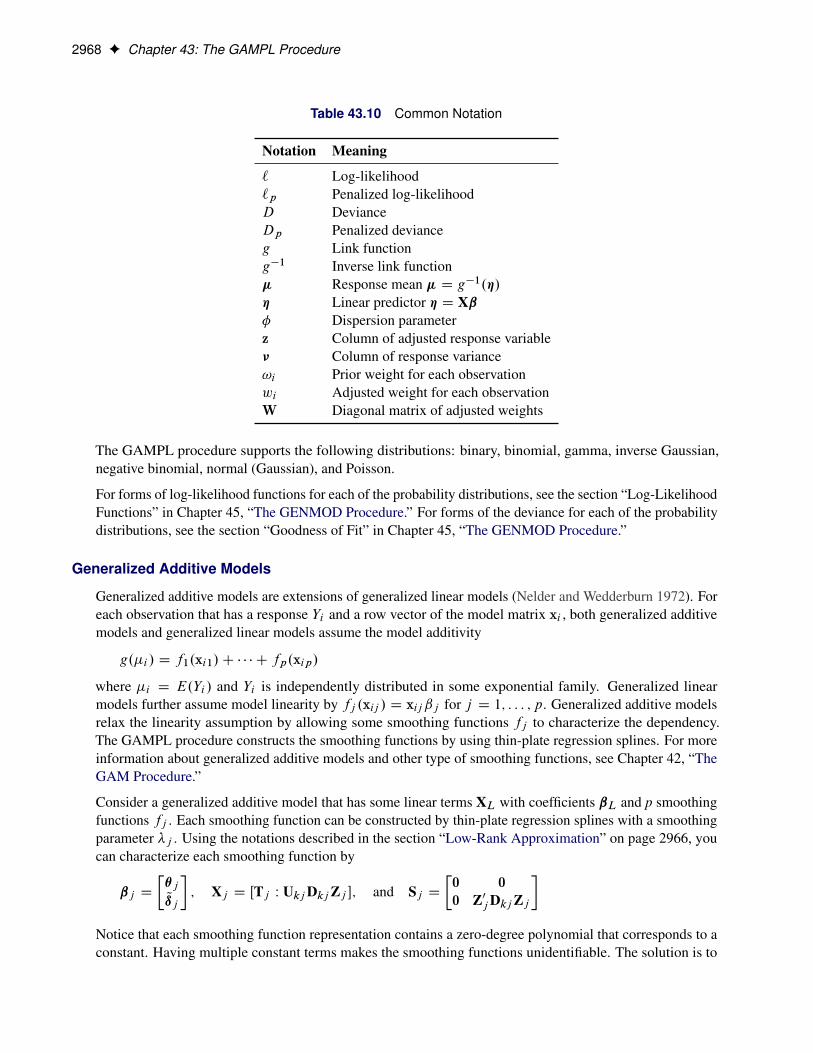
Table 43.10 lists and defines some common notation that is used in the context of generalized linear modelsand generalized additive models.
2968 F Chapter 43: The GAMPL Procedure
Table 43.10 Common Notation
Notation Meaning
` Log-likelihood`p Penalized log-likelihoodD DevianceDp Penalized devianceg Link functiong�1 Inverse link function� Response mean � D g�1.�/� Linear predictor � D Xˇ� Dispersion parameterz Column of adjusted response variable� Column of response variance!i Prior weight for each observationwi Adjusted weight for each observationW Diagonal matrix of adjusted weights
The GAMPL procedure supports the following distributions: binary, binomial, gamma, inverse Gaussian,negative binomial, normal (Gaussian), and Poisson.
For forms of log-likelihood functions for each of the probability distributions, see the section “Log-LikelihoodFunctions” in Chapter 45, “The GENMOD Procedure.” For forms of the deviance for each of the probabilitydistributions, see the section “Goodness of Fit” in Chapter 45, “The GENMOD Procedure.”
Generalized Additive Models
Generalized additive models are extensions of generalized linear models (Nelder and Wedderburn 1972). Foreach observation that has a response Yi and a row vector of the model matrix xi , both generalized additivemodels and generalized linear models assume the model additivity
g.�i / D f1.xi1/C � � � C fp.xip/
where �i D E.Yi / and Yi is independently distributed in some exponential family. Generalized linearmodels further assume model linearity by fj .xij / D xijˇj for j D 1; : : : ; p. Generalized additive modelsrelax the linearity assumption by allowing some smoothing functions fj to characterize the dependency.The GAMPL procedure constructs the smoothing functions by using thin-plate regression splines. For moreinformation about generalized additive models and other type of smoothing functions, see Chapter 42, “TheGAM Procedure.”
Consider a generalized additive model that has some linear terms XL with coefficients ˇL and p smoothingfunctions fj . Each smoothing function can be constructed by thin-plate regression splines with a smoothingparameter �j . Using the notations described in the section “Low-Rank Approximation” on page 2966, youcan characterize each smoothing function by
ˇj D
��jQıj
�; Xj D ŒTj W UkjDkjZj �; and Sj D
�0 00 Z0jDkjZj
�Notice that each smoothing function representation contains a zero-degree polynomial that corresponds to aconstant. Having multiple constant terms makes the smoothing functions unidentifiable. The solution is to

Model Evaluation Criteria F 2969
include a global constant term (that is, the intercept) in the model and enforce the centering constraint to eachsmoothing function. You can write the constraint as
10Xjˇj D 0
By using a similar approach as the linear constraint for thin-plate regression splines, you obtain the orthogonalcolumn basis Vj via the QR decomposition of X0j 1 such that 10XjVj D 0. Each smoothing function can bereparameterized as QXj D XjVj .
Let X D ŒXL W QX1 W � � � W QXp� and ˇ0 D Œˇ0L W ˇ01 W � � � W ˇ
0p�. Then the generalized additive model can be
represented as g.�/ D Xˇ. The roughness penalty matrix is represented as a block diagonal matrix:
S� D
26666666664
0 0 � � � 00 �1S1 � � � 0
: : ::::
::: �jSj:::
: : :
0 0 � � � �pSp
37777777775Then the roughness penalty is measured in the quadratic form ˇ0S�ˇ.
Penalized Likelihood Estimation
Given a fixed vector of smoothing parameters, � D Œ�i : : : �p�0, you can fit the generalized additive models bythe penalized likelihood estimation. In contrast to the maximum likelihood estimation, penalized likelihoodestimation obtains an estimate for ˇ by maximizing the penalized log likelihood,
`p.ˇ/ D `.ˇ/ �1
2ˇ0S�ˇ
Any optimization technique that you can use for maximum likelihood estimation can also be used forpenalized likelihood estimation. If first-order derivatives are required for the optimization technique, you cancompute the gradient as
@`p
@ˇD@`
@ˇ� S�ˇ
If second-order derivatives are required for the optimization technique, you can compute the Hessian as
@2`p
@ˇ@ˇ0D
@2`
@ˇ@ˇ0� S�
In the gradient and Hessian forms, @`=@ˇ and @2`=.@ˇ@ˇ0/ are the corresponding gradient and Hessian,respectively, for the log-likelihood for generalized linear models. For more information about optimizationtechniques, see the section “Choosing an Optimization Technique” on page 2975.
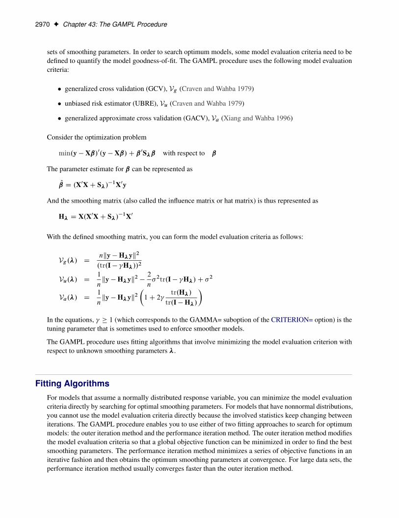
Model Evaluation CriteriaGiven a fixed set of smoothing parameters � in which each �i controls the smoothness of each spline term,you can fit a generalized additive model by the penalized likelihood estimation. There are infinitely many
2970 F Chapter 43: The GAMPL Procedure
sets of smoothing parameters. In order to search optimum models, some model evaluation criteria need to bedefined to quantify the model goodness-of-fit. The GAMPL procedure uses the following model evaluationcriteria:
� generalized cross validation (GCV), Vg (Craven and Wahba 1979)
� unbiased risk estimator (UBRE), Vu (Craven and Wahba 1979)
� generalized approximate cross validation (GACV), Va (Xiang and Wahba 1996)
Consider the optimization problem
min.y � Xˇ/0.y � Xˇ/C ˇ0S�ˇ with respect to ˇ
The parameter estimate for ˇ can be represented as
O D .X0XC S�/�1X0y
And the smoothing matrix (also called the influence matrix or hat matrix) is thus represented as
H� D X.X0XC S�/�1X0
With the defined smoothing matrix, you can form the model evaluation criteria as follows:
Vg.�/ Dnky �H�yk2
.tr.I � H�//2
Vu.�/ D1
nky �H�yk2 �
2
n�2tr.I � H�/C �
2
Va.�/ D1
nky �H�yk2
�1C 2
tr.H�/
tr.I �H�/
�In the equations, � 1 (which corresponds to the GAMMA= suboption of the CRITERION= option) is thetuning parameter that is sometimes used to enforce smoother models.
The GAMPL procedure uses fitting algorithms that involve minimizing the model evaluation criterion withrespect to unknown smoothing parameters �.
Fitting AlgorithmsFor models that assume a normally distributed response variable, you can minimize the model evaluationcriteria directly by searching for optimal smoothing parameters. For models that have nonnormal distributions,you cannot use the model evaluation criteria directly because the involved statistics keep changing betweeniterations. The GAMPL procedure enables you to use either of two fitting approaches to search for optimummodels: the outer iteration method and the performance iteration method. The outer iteration method modifiesthe model evaluation criteria so that a global objective function can be minimized in order to find the bestsmoothing parameters. The performance iteration method minimizes a series of objective functions in aniterative fashion and then obtains the optimum smoothing parameters at convergence. For large data sets, theperformance iteration method usually converges faster than the outer iteration method.

Fitting Algorithms F 2971
Outer Iteration (Experimental)
The outer iteration method is outlined in Wood (2006). The method uses modified model evaluation criteria,which are defined as follows:
Vog.�/ DnD�.�/
.n � tr.H�//2
Vou.�/ DD�.�/
n�2
n�2tr.I � H�/C �
2
Voa.�/ DD�.�/
nC2 tr.H�/P�
ntr.I �H�/
By replacing ky �H�yk2 with model deviance D�.�/, the modified model evaluation criteria relate to thesmoothing parameter � in a direct way such that the analytic gradient and Hessian are available in explicitforms. The Pearson’s statistic P� is used in the GACV criterion Voa.�/ (Wood 2008). The algorithm for theouter iteration is thus as follows:
1. Initialize smoothing parameters by taking one step of performance iteration based on adjusted responseand adjusted weight except for spline terms with initial values that are specified in the INITSMOOTH=option.
2. Search for the best smoothing parameters by minimizing the modified model evaluation criteria.The optimization process stops when any of the convergence criteria that are specified in theSMOOTHOPTIONS option is met. At each optimization step:
a) Initialize by setting initial regression parameters ˇ D fg. Oy/; 0; : : : ; 0g0. Set the initial dispersionparameter if necessary.
b) Search for the best regression parameters ˇ by minimizing the penalized deviance Dp (ormaximizing the penalized likelihood `p for negative binomial distribution). The optimizationprocess stops when any of the convergence criteria that are specified in the PLIKEOPTIONSoption is met.
c) At convergence, evaluate derivatives of the model evaluation criteria with respect to � by using@Dp=@ˇ, @2Dp=.@ˇ@ˇ0/, @ˇ=@�j , and @2ˇ=.@�j @�k/.
Step 2b usually converges quickly because it is essentially penalized likelihood estimation given thatDp D 2�.`max � `/C ˇS�ˇ
0. Step 2c contains involved computation by using the chain rule of derivatives.For more information about computing derivatives of Vog and Vou, see Wood (2008, 2011).
Performance Iteration
The performance iteration method is proposed by Gu and Wahba (1991). Wood (2004) modifies and stabilizesthe algorithm for fitting generalized additive models. The algorithm for the performance iteration method isas follows:
1. Initialize smoothing parameters � D f1; : : : ; 1g, except for spline terms whose initial values arespecified in the INITSMOOTH= option. Set the initial regression parameters ˇ D fg. Ny/; 0; : : : ; 0g0.Set the initial dispersion parameter if necessary.
2972 F Chapter 43: The GAMPL Procedure
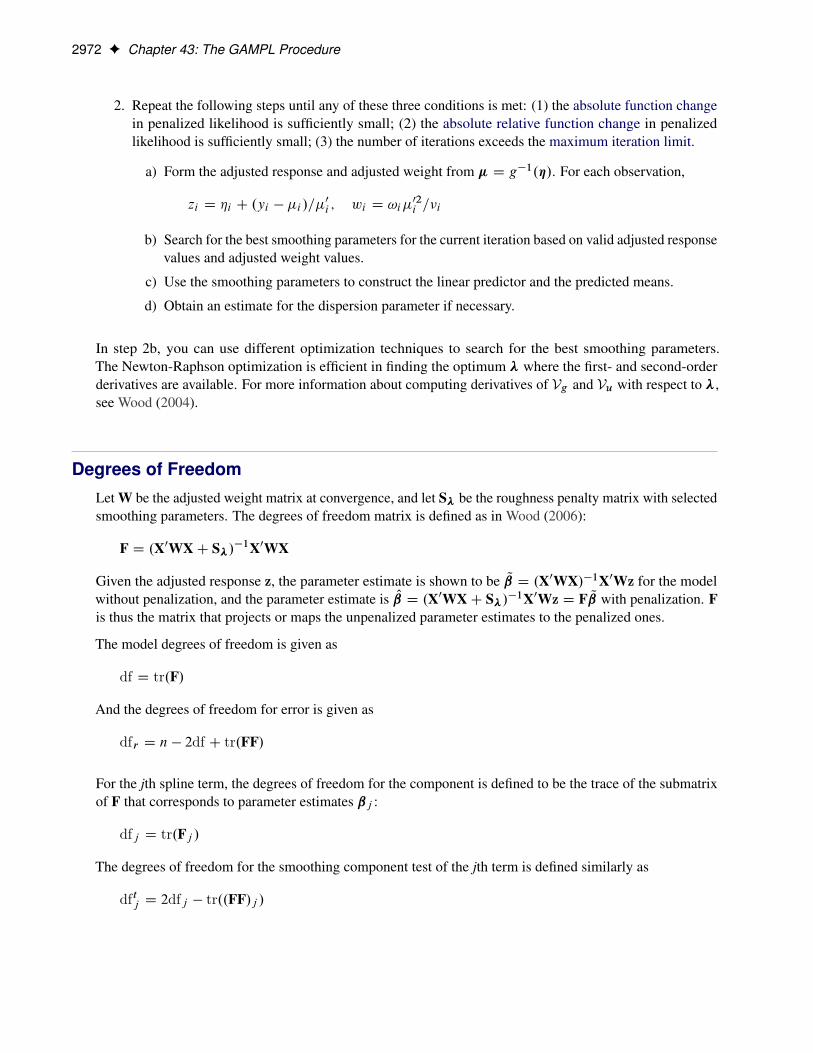
2. Repeat the following steps until any of these three conditions is met: (1) the absolute function changein penalized likelihood is sufficiently small; (2) the absolute relative function change in penalizedlikelihood is sufficiently small; (3) the number of iterations exceeds the maximum iteration limit.
a) Form the adjusted response and adjusted weight from � D g�1.�/. For each observation,
zi D �i C .yi � �i /=�0i ; wi D !i�
02i =�i
b) Search for the best smoothing parameters for the current iteration based on valid adjusted responsevalues and adjusted weight values.
c) Use the smoothing parameters to construct the linear predictor and the predicted means.
d) Obtain an estimate for the dispersion parameter if necessary.
In step 2b, you can use different optimization techniques to search for the best smoothing parameters.The Newton-Raphson optimization is efficient in finding the optimum � where the first- and second-orderderivatives are available. For more information about computing derivatives of Vg and Vu with respect to �,see Wood (2004).
Degrees of FreedomLet W be the adjusted weight matrix at convergence, and let S� be the roughness penalty matrix with selectedsmoothing parameters. The degrees of freedom matrix is defined as in Wood (2006):
F D .X0WXC S�/�1X0WX
Given the adjusted response z, the parameter estimate is shown to be Q D .X0WX/�1X0Wz for the modelwithout penalization, and the parameter estimate is O D .X0WXC S�/
�1X0Wz D F Q with penalization. Fis thus the matrix that projects or maps the unpenalized parameter estimates to the penalized ones.
The model degrees of freedom is given as
df D tr.F/
And the degrees of freedom for error is given as
dfr D n � 2df C tr.FF/
For the jth spline term, the degrees of freedom for the component is defined to be the trace of the submatrixof F that corresponds to parameter estimates ˇj :
dfj D tr.Fj /
The degrees of freedom for the smoothing component test of the jth term is defined similarly as
dftj D 2dfj � tr..FF/j /

Model Inference F 2973
Model InferenceWahba (1983) proposes a Bayesian covariance matrix for parameter estimates ˇ by interpreting a smoothingspline as a posterior mean. Nychka (1988) shows that the derived Bayesian posterior confidence limits workwell from frequentist viewpoints. The Bayesian posterior covariance matrix for the parameters is
Vˇ D .X0WXC S�/�1�2
The posterior distribution for ˇ is thus
ˇjy � N. O;Vˇ/
For a particular point whose design row is vector x, the prediction is x O and the standard error isp
xVˇx0.The Bayesian posterior confidence limits are thus�
x O ˙ z˛=2q
xVˇx0�
where z˛=2 is the 1 � ˛=2 quantile of the standard normal distribution.
For the jth spline term, the prediction for the component is formed by xj O, where xj is a row vector of zerosexcept for columns that correspond to basis expansions of the jth spline term. And the standard error for thecomponent is
qxjVˇx0j .
Dispersion ParameterSome distribution families (Gaussian, gamma, inverse Gaussian, and negative binomial) have a dispersionparameter that you can specify in the DISPERSION= option in the MODEL statement or you can estimatefrom the data. The following three suboptions for the SCALE= option in the MODEL statement correspondto three ways to estimate the dispersion parameter:
DEVIANCEestimates the dispersion parameter by the deviance, given the regression parameter estimates:
O� D
Pi Di .yi ; �i /
n � df
MLEestimates the dispersion parameter by maximizing the penalized likelihood, given the regressionparameter estimates:
O� D argmax�
`p. O; �/
The MLE option is the only option that you can use to estimate the dispersion parameter for thenegative binomial distribution.
PEARSONestimates the dispersion parameter by Pearson’s statistic, given the regression parameter estimates:
O� D
Pi !i .yi � �i /
2=�i
n � df
If the dispersion parameter is estimated, it contributes one additional degree of freedom to the fitted model.

2974 F Chapter 43: The GAMPL Procedure
Tests for Smoothing ComponentsThe GAMPL procedure performs a smoothing component test on the null hypotheses fj D 0 for the jthcomponent. In contrast to the analysis of deviance that is used in PROC GAM (which tests existence ofnonlinearity for each smoothing component), the smoothing component test used in PROC GAMPL tests forthe existence of a contribution for each smoothing component.
The hypothesis test is based on the Wald statistic. Define Xj as the matrix of all zeros except for columns thatcorrespond to basis expansions of the jth spline term. Then the column vector of predictions is Ofj D Xj O,and the covariance matrix for the predictions is Vj D XjVˇX0j . The Wald statistic for testing is
Tr D Of 0jVr�j Ofj D O0X0j .XjVˇX0j /
r�Xj O
where Vr�j is the rank-r pseudo-inverse of Vj . If Rj is the Cholesky root for X0jXj such that R0jR D X0jXj ,then the test statistic can be written as
Tr D O0R0j .RjVˇR0j /
r�Rj O
Wood (2012) proposes using the dftj degrees of freedom for test (which is defined in the section “Degrees ofFreedom” on page 2972) as the rank r. Because spline terms in fitted models often have noninteger degreesof freedom, the GAMPL procedure uses a rounded value of dftj as the rank:
r D
(bdftj c if dftj � bdftj c <D 0:05 or dftj < 1ddftj e otherwise
Let K be a symmetric and nonnegative definite matrix, and let its eigenvalues be sorted as d1 > d2 > � � � ;then the rank-r pseudo-inverse of K is formed by
Kr� D Uk
264d�11
: : :
d�1r
375U 0kwhere Uk are formed by columns of eigenvectors that correspond to the r eigenvalues.
Under the null hypothesis, the Wald statistic Tr approximately follows the chi-square distribution Tr � �2r .For an observed test statistic tr , the p-value for rejecting the null hypothesis is computed as P.�2r > tr/ ifthe dispersion parameter is constant, or P.Fr;dfr > tr/ with dfr error degrees of freedom if the dispersionparameter is estimated.
Be cautious when you interpret the results of the smoothing component test because p-values are computedby approximation and the test does not take the smoothing parameter selection process into account.
Computational Method: MultithreadingThreading is the organization of computational work into multiple tasks (processing units that can bescheduled by the operating system). Each task is associated with a thread. Multithreading is the concurrentexecution of threads. When multithreading is possible, you can realize substantial performance gainscompared to the performance you get from sequential (single-threaded) execution.
The number of threads that the GAMPL procedure spawns is determined by the number of CPUs on amachine and can be controlled in the following ways:

Choosing an Optimization Technique F 2975
� You can specify the number of CPUs in the CPUCOUNT= SAS system option. For example, if youspecify the following statement, the GAMPL procedure determines threading as if it were executingon a system that had four CPUs, regardless of the actual CPU count:
options cpucount=4;
� You can specify the NTHREADS= option in the PERFORMANCE statement to control the number ofthreads. This specification overrides the CPUCOUNT= system option. Specify NTHREADS=1 toforce single-threaded execution.
The GAMPL procedure allocates one thread per CPU by default.
The tasks that are multithreaded by the GAMPL procedure are primarily defined by dividing the data that areprocessed on a single machine among the threads—that is, the GAMPL procedure implements multithreadingthrough a data-parallel model. For example, if the input data set has 1,000 observations and PROC GAMPLis running with four threads, then 250 observations are associated with each thread. All operations thatrequire access to the data are then multithreaded. These operations include the following:
� variable levelization
� effect levelization
� formation of the initial crossproducts matrix
� truncated eigendecomposition
� formation of spline basis expansions
� objective function calculation
� gradient calculation
� Hessian calculation
� scoring of observations
� computing predictions for smoothing component plots
In addition, operations on matrices such as sweeps can be multithreaded if the matrices are of sufficient sizeto realize performance benefits from managing multiple threads for the particular matrix operation.
Choosing an Optimization Technique
First- or Second-Order Techniques
The factors that affect how you choose an optimization technique for a particular problem are complex.Although the default technique works well for most problems, you might occasionally benefit from tryingseveral different techniques.

2976 F Chapter 43: The GAMPL Procedure
For many optimization problems, computing the gradient takes more computer time than computing thefunction value. Computing the Hessian sometimes takes much more computer time and memory thancomputing the gradient, especially when there are many decision variables. Unfortunately, optimizationtechniques that do not use some kind of Hessian approximation usually require many more iterations thantechniques that use a Hessian matrix; as a result, the total run time of these techniques is often longer.Techniques that do not use the Hessian also tend to be less reliable. For example, they can terminate moreeasily at stationary points than at global optima.
Table 43.11 shows which derivatives are required for each optimization technique.
Table 43.11 Derivatives Required
Technique First-Order Second-Order
TRUREG x xNEWRAP x xNRRIDG x xQUANEW x -DBLDOG x -CONGRA x -NMSIMP - -
The second-order derivative techniques (TRUREG, NEWRAP, and NRRIDG) are best for small problems forwhich the Hessian matrix is not expensive to compute. Sometimes the NRRIDG technique can be faster thanthe TRUREG technique, but TRUREG can be more stable. The NRRIDG technique requires only one matrixwith p.p C 1/=2 double words, where p denotes the number of parameters in the optimization. TRUREGand NEWRAP require two such matrices.
The QUANEW and DBLDOG first-order derivative techniques are best for medium-sized problems forwhich the objective function and the gradient can be evaluated much faster than the Hessian. In general, theQUANEW and DBLDOG techniques require more iterations than TRUREG, NRRIDG, and NEWRAP, buteach iteration can be much faster. The QUANEW and DBLDOG techniques require only the gradient toupdate an approximate Hessian, and they require slightly less memory than TRUREG or NEWRAP.
The CONGRA first-order derivative technique is best for large problems for which the objective functionand the gradient can be computed much faster than the Hessian and for which too much memory is requiredto store the (approximate) Hessian. In general, the CONGRA technique requires more iterations thanQUANEW or DBLDOG, but each iteration can be much faster. Because CONGRA requires only a factor ofp double-word memory, many large applications can be solved only by CONGRA.
The no-derivative technique NMSIMP is best for small problems for which derivatives are not continuous orare very difficult to compute.
Each optimization technique uses one or more convergence criteria that determine when it has converged. Atechnique is considered to have converged when any one of the convergence criteria is satisfied. For example,under the default settings, the QUANEW technique converges if the value of the ABSGCONV= option isless than 1E–5, the value of the FCONV= option is less than 2 � �, or the value of the GCONV= option isless than 1E–8.
By default, the GAMPL procedure applies the NEWRAP technique to optimization for selecting smoothingparameters by using the performance iteration method. For the outer iteration method, the GAMPL procedure

Choosing an Optimization Technique F 2977
applies the QUANEW technique for selecting smoothing parameters.
Technique Descriptions
The following subsections provide details about each optimization technique and follow the same order asTable 43.11.
Trust Region Optimization (TRUREG)The trust region technique (TRUREG) uses the gradient g. .k// and the Hessian matrix H. .k//; thus,it requires that the objective function f . / have continuous first- and second-order derivatives inside thefeasible region.
The trust region technique iteratively optimizes a quadratic approximation to the nonlinear objective functionwithin a hyperelliptic trust region that has radius� and constrains the step size that corresponds to the qualityof the quadratic approximation. The trust region technique that PROC GAMPL uses is based on Dennis, Gay,and Welsch (1981); Gay (1983); Moré and Sorensen (1983).
The trust region technique performs well for small- to medium-sized problems, and it does not need manyfunction, gradient, and Hessian calls. However, if the computation of the Hessian matrix is computationallyexpensive, either the QUANEW technique or the CONGRA technique might be more efficient.
Newton-Raphson Optimization with Line Search (NEWRAP)The Newton-Raphson optimization with line search (NEWRAP) technique uses the gradient g. .k// and theHessian matrix H. .k//; thus, it requires that the objective function have continuous first- and second-orderderivatives inside the feasible region.
If second-order derivatives are computed efficiently and precisely, the NEWRAP technique can perform wellfor medium-sized to large problems, and it does not need many function, gradient, and Hessian calls.
This technique uses a pure Newton step when the Hessian is positive-definite and when the Newton stepreduces the value of the objective function successfully. Otherwise, a combination of ridging and line searchis performed to compute successful steps. If the Hessian is not positive-definite, a multiple of the identitymatrix is added to the Hessian matrix to make it positive-definite (Eskow and Schnabel 1991).
In each iteration, a line search is performed along the search direction to find an approximate optimum of theobjective function. The line-search technique uses quadratic interpolation and cubic extrapolation.
Newton-Raphson Ridge Optimization (NRRIDG)The Newton-Raphson ridge optimization (NRRIDG) technique uses the gradient g. .k// and the Hessianmatrix H. .k//; thus, it requires that the objective function have continuous first- and second-order derivativesinside the feasible region.
This technique uses a pure Newton step when the Hessian is positive-definite and when the Newton stepreduces the value of the objective function successfully. If at least one of these two conditions is not satisfied,a multiple of the identity matrix is added to the Hessian matrix.
Because the NRRIDG technique uses an orthogonal decomposition of the approximate Hessian, each iterationof NRRIDG can be slower than an iteration of the NEWRAP technique, which works with a Choleskydecomposition. However, NRRIDG usually requires fewer iterations than NEWRAP.

2978 F Chapter 43: The GAMPL Procedure
The NRRIDG technique performs well for small- to medium-sized problems, and it does not require manyfunction, gradient, and Hessian calls. However, if the computation of the Hessian matrix is computationallyexpensive, either the QUANEW technique or the CONGRA technique might be more efficient.
Dual Quasi-Newton Optimization (QUANEW)The dual quasi-Newton (QUANEW) technique uses the gradient g. .k//, and it does not need to computesecond-order derivatives, because they are approximated. It works well for medium-sized to moderatelylarge optimization problems, where the objective function and the gradient can be computed much fasterthan the Hessian. However, the QUANEW technique requires more iterations in general than the TRUREG,NEWRAP, and NRRIDG techniques, which compute second-order derivatives. The QUANEW techniqueprovides an appropriate balance between the speed and stability that are required for most generalized linearmodel applications.
The QUANEW technique that PROC GAMPL uses is the dual quasi-Newton technique, which updates theCholesky factor of an approximate Hessian.
In each iteration, a line search is performed along the search direction to find an approximate optimum. Theline-search technique uses quadratic interpolation and cubic extrapolation to obtain a step size ˛ that satisfiesthe Goldstein conditions (Fletcher 1987). One of the Goldstein conditions can be violated if the feasibleregion defines an upper limit of the step size. Violating the left-side Goldstein condition can affect thepositive-definiteness of the quasi-Newton update. In that case, either the update is skipped or the iterationsare restarted by using an identity matrix, resulting in the steepest descent or ascent search direction.
Double-Dogleg Optimization (DBLDOG)The double-dogleg optimization (DBLDOG) technique combines the ideas of the quasi-Newton and trustregion techniques. In each iteration, the double-dogleg technique computes the step s.k/ as the linearcombination of the steepest descent or ascent search direction s.k/1 and a quasi-Newton search direction s.k/2 :
s.k/ D ˛1s.k/1 C ˛2s
.k/2
The step must remain within a prespecified trust region radius (Fletcher 1987, p. 107). Thus, the DBLDOGsubroutine uses the dual quasi-Newton update but does not perform a line search.
The double-dogleg optimization technique works well for medium-sized to moderately large optimizationproblems, where the objective function and the gradient can be computed much faster than the Hessian.The implementation is based on Dennis and Mei (1979) and Gay (1983), but it is extended for dealingwith boundary and linear constraints. The DBLDOG technique generally requires more iterations than theTRUREG, NEWRAP, and NRRIDG techniques, which require second-order derivatives; however, each of theDBLDOG iterations is computationally cheap. Furthermore, the DBLDOG technique requires only gradientcalls for updating of the Cholesky factor of an approximate Hessian.
Conjugate Gradient Optimization (CONGRA)Second-order derivatives are not required by the CONGRA technique and are not even approximated. TheCONGRA technique can be expensive in function and gradient calls, but it requires only O.p/ memoryfor unconstrained optimization. In general, the technique must perform many iterations to obtain a precisesolution, but each of the CONGRA iterations is computationally cheap.
The CONGRA technique should be used for optimization problems that have large p. For the unconstrained orboundary-constrained case, the CONGRA technique requires only O.p/ bytes of working memory, whereasall other optimization techniques require order O.p2/ bytes of working memory. During p successive

Displayed Output F 2979
iterations that are uninterrupted by restarts or changes in the working set, the CONGRA technique computesa cycle of p conjugate search directions. In each iteration, a line search is performed along the searchdirection to find an approximate optimum of the objective function. The line-search technique uses quadraticinterpolation and cubic extrapolation to obtain a step size ˛ that satisfies the Goldstein conditions. One of theGoldstein conditions can be violated if the feasible region defines an upper limit for the step size.
Nelder-Mead Simplex Optimization (NMSIMP)The Nelder-Mead simplex technique does not use any derivatives and does not assume that the objectivefunction has continuous derivatives. The objective function itself needs to be continuous. This technique isquite expensive in the number of function calls, and it might be unable to generate precise results for p � 40.
The original Nelder-Mead simplex technique is implemented and extended to boundary constraints. Thistechnique does not compute the objective for infeasible points, but it changes the shape of the simplex andadapts to the nonlinearities of the objective function. This change contributes to an increased speed ofconvergence and uses a special termination criterion.
Displayed OutputThe following sections describe the output that the GAMPL procedure produces by default. The output isorganized into various tables, which are discussed in the order of their appearance.
Performance Information
The “Performance Information” table is produced by default. It displays information about the executionmode. For single-machine mode, the table displays the number of threads used. For distributed mode, thetable displays the grid mode (symmetric or asymmetric), the number of compute nodes, and the number ofthreads per node.
If you specify the DETAILS option in the PERFORMANCE statement, PROC GAMPL also produces a“Timing” table, which displays elapsed times (absolute and relative) for the main tasks of the procedure.
Data Access Information
The “Data Access Information” table is produced by default. For the input and output data sets, it displaysthe libref and data set name, the engine that was used to access the data, the role (input or output) of the dataset, and the path that the data followed to reach the computation.
Model Information
The “Model Information” table displays basic information about the model, such as the response variable,frequency variable, link function, and model category that the GAMPL procedure determines based onyour input and options. The “Model Information” table also displays the distribution of the data thatPROC GAMPL assumes. For information about the supported response distributions, see the section“DISTRIBUTION=keyword” on page 2960.
2980 F Chapter 43: The GAMPL Procedure
Number of Observations
The “Number of Observations” table displays the number of observations that are read from the input dataset and the number of observations that are used in the analysis. If a FREQ statement is present, the sum ofthe frequencies read and used is displayed. If the events/trials syntax is used, the number of events and trialsis also displayed.
Response Profile
The “Response Profile” table displays the ordered values from which the GAMPL procedure determines theprobability that is modeled as an event in binary models. For each response category level, the frequencythat is used in the analysis is reported. You can affect the ordering of the response values by specifyingresponse-options in the MODEL statement. For binary models, the note that follows the “Response Profile”table indicates which outcome is modeled as the event in binary models and which value serves as thereference category.
The “Response Profile” table is not produced for binomial (events/trials) data. You can find informationabout the number of events and trials in the “Number of Observations” table.
Class Level Information
The “Class Level Information” table lists the levels of every variable that is specified in the CLASS statement.You should check this information to make sure that the data are correct. You can adjust the order of theCLASS variable levels by specifying the ORDER= option in the CLASS statement. You can suppress the“Class Level Information” table completely or partially by specifying the NOCLPRINT= option in the PROCGAMPL statement.
If the classification variables use reference parameterization, the “Class Level Information” table also displaysthe reference value for each variable.
Specifications for Spline(spline-variables)
The “Specifications for Spline(spline-variables)” table displays basic information (such as number ofvariables, specified degrees of freedom, search range for the smoothing parameter, and so on) about howto construct a spline term that the GAMPL procedure uses to construct basis expansions and search for thesmoothing parameter. PROC GAMPL generates the “Specifications for Spline(spline-variables)” table onlywhen you specify the DETAILS option for a spline term.
Optimization Iteration History
For each iteration of the optimization, the “Iteration History” table displays the number of function evaluations(including gradient and Hessian evaluations), the value of the objective function, the change in the objectivefunction from the previous iteration, and the absolute value of the largest (projected) gradient element.The objective function that PROC GAMPL uses in the optimization is normalized by default to enablecomparisons across data sets that have different sampling intensity.
If you specify the ITDETAILS option in the PROC GAMPL statement, information about the parameterestimates and gradients in the course of the optimization is added to the “Iteration History” table.
For a parametric generalized linear model or for a generalized additive model that has fixed smoothingparameters, the “Iteration History” table displays information about regression parameter estimates and

Displayed Output F 2981
gradients. For a generalized additive model that has unknown smoothing parameters, the “Iteration History”table displays information about smoothing parameter estimates and gradients. If the performance iterationmethod is used, a column of performance iteration steps is added to the table.
Convergence Status
The convergence status table is a small ODS table that follows the “Iteration History” table in the defaultoutput. In the listing, this table appears as a message that indicates whether the optimization succeeded andwhich convergence criterion was met. If the optimization fails, the message indicates the reason for thefailure. If you save the convergence status table to an output data set, a numeric Status variable is added thatenables you to programmatically assess convergence. The values of the Status variable encode the following:
0 Convergence was achieved, or an optimization was not performed because TECHNIQUE=NONEwas specified.
1 The objective function could not be improved.
2 Convergence was not achieved because of a user interrupt or because a limit (such as the maximumnumber of iterations or the maximum number of function evaluations) was reached. To modifythese limits, see the MAXITER=, MAXFUNC=, and MAXTIME= options in the PROC GAMPLstatement.
3 Optimization failed to converge because function or derivative evaluations failed at the startingvalues or during the iterations or because a feasible point that satisfies the parameter constraintscould not be found in the parameter space.
Fit Statistics
The “Fit Statistics” table displays a variety of likelihood-based measures of fit in addition to the modelroughness measurement. All information criteria are presented in “smaller is better” form.
The calculation of the information criteria uses the following formulas, where df denotes the model degreesof freedom, f denotes the number of frequencies used, and ` is the log likelihood that is evaluated at theconverged estimates:
AIC D� 2`C 2df
AICC D��2`C 2dff=.f � df � 1/ when f > df C 2�2`C 2df.df C 2/ otherwise
BIC D� 2`C df log.f /
If no FREQ statement is specified, then f equals n, the number of observations that are used.
Parameter Estimates
The “Parameter Estimates” table displays the regression parameter estimates, their estimated (asymptotic)standard errors, chi-square statistics, and p-values for the hypothesis that the parameter is 0.
Estimates for Smoothing Components
The “Estimates for Smoothing Components” table displays a summary of the fitted spline terms, includingeffective degrees of freedom, smoothing parameters, roughness penalty values, number of parameters, rankof penalty matrix, and number of knots.
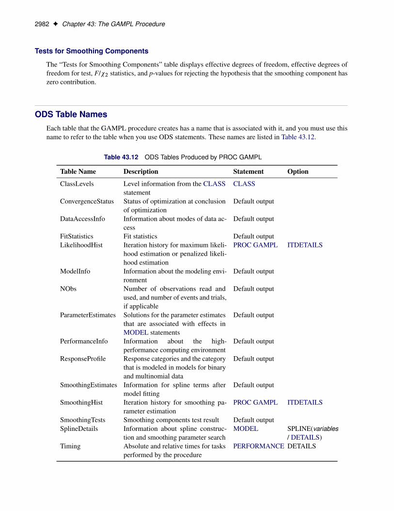
2982 F Chapter 43: The GAMPL Procedure
Tests for Smoothing Components
The “Tests for Smoothing Components” table displays effective degrees of freedom, effective degrees offreedom for test, F/�2 statistics, and p-values for rejecting the hypothesis that the smoothing component haszero contribution.
ODS Table NamesEach table that the GAMPL procedure creates has a name that is associated with it, and you must use thisname to refer to the table when you use ODS statements. These names are listed in Table 43.12.
Table 43.12 ODS Tables Produced by PROC GAMPL
Table Name Description Statement Option
ClassLevels Level information from the CLASSstatement
CLASS
ConvergenceStatus Status of optimization at conclusionof optimization
Default output
DataAccessInfo Information about modes of data ac-cess
Default output
FitStatistics Fit statistics Default outputLikelihoodHist Iteration history for maximum likeli-
hood estimation or penalized likeli-hood estimation
PROC GAMPL ITDETAILS
ModelInfo Information about the modeling envi-ronment
Default output
NObs Number of observations read andused, and number of events and trials,if applicable
Default output
ParameterEstimates Solutions for the parameter estimatesthat are associated with effects inMODEL statements
Default output
PerformanceInfo Information about the high-performance computing environment
Default output
ResponseProfile Response categories and the categorythat is modeled in models for binaryand multinomial data
Default output
SmoothingEstimates Information for spline terms aftermodel fitting
Default output
SmoothingHist Iteration history for smoothing pa-rameter estimation
PROC GAMPL ITDETAILS
SmoothingTests Smoothing components test result Default outputSplineDetails Information about spline construc-
tion and smoothing parameter searchMODEL SPLINE(variables
/ DETAILS)Timing Absolute and relative times for tasks
performed by the procedurePERFORMANCE DETAILS

Examples: GAMPL Procedure F 2983
By referring to the names of such tables, you can use the ODS OUTPUT statement to place one or more ofthese tables in output data sets.
ODS GraphicsStatistical procedures use ODS Graphics to create graphs as part of their output. ODS Graphics is describedin detail in Chapter 21, “Statistical Graphics Using ODS.”
Before you create graphs, ODS Graphics must be enabled (for example, by specifying the ODS GRAPH-ICS ON statement). For more information about enabling and disabling ODS Graphics, see the section“Enabling and Disabling ODS Graphics” on page 607 in Chapter 21, “Statistical Graphics Using ODS.”
The overall appearance of graphs is controlled by ODS styles. Styles and other aspects of using ODSGraphics are discussed in the section “A Primer on ODS Statistical Graphics” on page 606 in Chapter 21,“Statistical Graphics Using ODS.”
When ODS Graphics is enabled, the GAMPL procedure by default produces plots of the partial predictionsfor each spline term in the model. Use the PLOTS option in the PROC GAMPL statement to control aspectsof these plots.
PROC GAMPL assigns a name to each graph that it creates by using ODS. You can use these names to referto the graphs when using ODS. The names are listed in Table 43.13.
Table 43.13 Graphs Produced by PROC GAMPL
ODS Graph Name Plot Description PLOTS= Option
SmoothingComponentPanel Panel of multiple prediction curves DefaultCOMPONENTS
SmoothingComponentPlot Unpacked prediction curves PLOTS(UNPACK)PLOTS=COMPONENTS(UNPACK)
By default, prediction plots for each spline component are displayed in panels that contain at most six plots.If you specify more than six smoothing components, multiple panels are used. Use the PLOTS(UNPACK)option in the PROC GAMPL statement to display these plots individually.
Examples: GAMPL Procedure
Example 43.1: Scatter Plot SmoothingThis example shows how you can use PROC GAMPL to perform scatter plot smoothing.
The example uses the LIDAR data set (Ruppert, Wand, and Carroll 2003). This data set is used in manybooks and journals to illustrate different smoothing techniques. Scientists use a technique known as LIDAR

2984 F Chapter 43: The GAMPL Procedure
(light detection and ranging), which uses laser reflections to detect chemical compounds in the atmosphere.The following DATA step creates the data set Lidar:
title 'Scatter Plot Smoothing';data Lidar;
input Range LogRatio @@;datalines;
390 -0.05035573 391 -0.06009706 393 -0.04190091 394 -0.0509847396 -0.05991345 397 -0.02842392 399 -0.05958421 400 -0.03988881402 -0.02939582 403 -0.03949445 405 -0.04764749 406 -0.06038408 -0.03123034 409 -0.03816584 411 -0.07562269 412 -0.05001751414 -0.0457295 415 -0.07766966 417 -0.02460641 418 -0.07133184
... more lines ...
702 -0.4716702 703 -0.7801088 705 -0.6668431 706 -0.5783479708 -0.7874522 709 -0.6156956 711 -0.8967602 712 -0.7077379714 -0.672567 715 -0.6218413 717 -0.8657611 718 -0.557754720 -0.8026684;
In this data set, Range records the distance that light travels before it is reflected back to the source. LogRatiois the logarithm of the ratio of light that is received from two laser sources. The objective is to use scatterplot smoothing to discover the nonlinear pattern in the data set. SAS provides different methods (for examplelocal regression) for scatter plot smoothing. You can perform scatter plot smoothing by using the SGPLOTprocedure, as shown in the following statements:
proc sgplot data=Lidar;scatter x=Range y=LogRatio;loess x=Range y=LogRatio / nomarkers;pbspline x=Range y=LogRatio / nomarkers;
run;
Output 43.1.1 shows the scatter plot of Range and LogRatio and the smoothing curves that are fitted by localregression and penalized B-splines smoothing techniques.

Example 43.1: Scatter Plot Smoothing F 2985
Output 43.1.1 Scatter Plot Smoothing
Both scatter plot smoothing techniques show a significant nonlinear structure between Range and LogRatiothat cannot be easily modeled by ordinary polynomials. You can also use the GAMPL procedure to performscatter plot smoothing on this data set, as in the following statements:
proc gampl data=Lidar seed=12345;model LogRatio = spline(Range/details);output out=LidarOut pred=p;
run;
The “Specifications for Spline(Range)” table in Output 43.1.2 displays the specifications for constructingthe spline term for Range. The maximum degrees of freedom is 10, which sets the upper limit of effectivedegrees of freedom for the spline term to be 9 after one degree of freedom is absorbed in the intercept. Theorder of the derivative in the penalty is 2, which means the unpenalized portion of the spline term involvespolynomials with degrees up to 2.

2986 F Chapter 43: The GAMPL Procedure
Output 43.1.2 Spline Specification
Scatter Plot Smoothing
The GAMPL Procedure
Scatter Plot Smoothing
The GAMPL Procedure
Specifications for Spline(Range)
Number of Variables 1
Rank of Penalty Approximation 10
Order of Derivative in the Penalty 2
Maximum Number of Knots 2000
The “Fit Statistics” table in Output 43.1.3 shows the summary statistics for the fitted model.
Output 43.1.3 Fit Statistics
Fit Statistics
Penalized Log Likelihood 251.44124
Roughness Penalty 0.00000426
Effective Degrees of Freedom 9.99988
Effective Degrees of Freedom for Error 211.00000
AIC (smaller is better) -482.88271
AICC (smaller is better) -481.83512
BIC (smaller is better) -448.90148
GCV (smaller is better) 0.00654
The “Estimates for Smoothing Components” table in Output 43.1.4 shows that the effective degrees offreedom for the spline term of Range is approximately 8 after the GCV criterion is optimized with respect tothe smoothing parameter. The roughness penalty is small, suggesting that there is an important contributionfrom the penalized part of thin-plate regression splines beyond nonpenalized polynomials.
Output 43.1.4 Estimates for Smoothing Components
Estimates for Smoothing Components
ComponentEffective
DFSmoothingParameter
RoughnessPenalty
Number ofParameters
Rank ofPenalty
MatrixNumber of
Knots
Spline(Range) 7.99988 1.0000 4.263E-6 9 10 221
Because the optimal model is obtained by searching in a functional space that is constrained by the maximumdegrees of freedom for a spline term, you might wonder whether PROC GAMPL produces a much differentmodel if you increase the value. The following statements fit another model in which the maximum degreesof freedom is increased to 20:
proc gampl data=Lidar seed=12345;model LogRatio = spline(Range/maxdf=20);output out=LidarOut2 pred=p2;
run;

Example 43.1: Scatter Plot Smoothing F 2987
Output 43.1.5 displays fit summary statistics for the second model. The model fit statistics from the secondmodel are very close to the ones from the first model, indicating that the second model is not much differentfrom the first model.
Output 43.1.5 Fit Statistics
Scatter Plot Smoothing
The GAMPL Procedure
Scatter Plot Smoothing
The GAMPL Procedure
Fit Statistics
Penalized Log Likelihood 250.95136
Roughness Penalty 0.06254
Effective Degrees of Freedom 10.04384
Effective Degrees of Freedom for Error 209.03211
AIC (smaller is better) -481.87757
AICC (smaller is better) -480.82094
BIC (smaller is better) -447.74696
GCV (smaller is better) 0.00657
Output 43.1.6 shows that the effective degrees of freedom for the spline term of Range is slightly largerthan 8, which is understandable because increasing the maximum degrees of freedom expands the functionalspace for model searching. Functions in the expanded space can provide a better fit to the data, but they arealso penalized more because the roughness penalty value for the second model is much larger than the onefor the first model. This suggests that functions in the expanded space do not help much, given the nonlinearrelationship between Range and LogRatio.
Output 43.1.6 Estimates for Smoothing Components
Estimates for Smoothing Components
ComponentEffective
DFSmoothingParameter
RoughnessPenalty
Number ofParameters
Rank ofPenalty
MatrixNumber of
Knots
Spline(Range) 8.04384 23134.6 0.0625 19 20 221
The two fitted models are all based on thin-plate regression splines, in which polynomials that have degreeshigher than 2 are penalized. You might wonder whether allowing higher-order polynomials yields a muchdifferent model. The following statements fit a third spline model by penalizing polynomials that havedegrees higher than 3:
proc gampl data=Lidar seed=12345;model LogRatio = spline(Range/m=3);output out=LidarOut3 pred=p3;
run;
The fit summary statistics shown in Output 43.1.7 are close to the ones from the previous two models, albeitslightly smaller.

2988 F Chapter 43: The GAMPL Procedure
Output 43.1.7 Fit Statistics
Scatter Plot Smoothing
The GAMPL Procedure
Scatter Plot Smoothing
The GAMPL Procedure
Fit Statistics
Penalized Log Likelihood 249.79779
Roughness Penalty 9.440383E-9
Effective Degrees of Freedom 10.00000
Effective Degrees of Freedom for Error 211.00000
AIC (smaller is better) -479.59559
AICC (smaller is better) -478.54797
BIC (smaller is better) -445.61397
GCV (smaller is better) 0.00664
As shown in Output 43.1.8, the effective degrees of freedom for the spline term where polynomials withdegrees less than 4 are allowed without penalization is 8. The roughness penalty is quite small compared tothe previous two fits. This also suggests that there are important contributions from the penalized part of thethin-plate regression splines even after the nonpenalized polynomials are raised to order 3.
Output 43.1.8 Estimates for Smoothing Components
Estimates for Smoothing Components
ComponentEffective
DFSmoothingParameter
RoughnessPenalty
Number ofParameters
Rank ofPenalty
MatrixNumber of
Knots
Spline(Range) 8.00000 1.0000 9.44E-9 9 10 221
The following statements use the DATA step to merge the predictions from the three scatter plot smoothingfits by PROC GAMPL and use the SGPLOT procedure to visualize them:
data LidarPred;merge Lidar LidarOut LidarOut2 LidarOut3;
run;
proc sgplot data=LidarPred;scatter x=Range y=LogRatio / markerattrs=GraphData1(size=7);series x=Range y=p / lineattrs =GraphData2(thickness=2)
legendlabel="Spline 1";series x=Range y=p2 / lineattrs =GraphData3(thickness=2)
legendlabel="Spline 2";series x=Range y=p3 / lineattrs =GraphData4(thickness=2)
legendlabel="Spline 3";run;
Output 43.1.9 displays the scatter plot smoothing fits by PROC GAMPL under three different splinespecifications.

Example 43.2: Nonparametric Logistic Regression F 2989
Output 43.1.9 Scatter Plot Smoothing
Example 43.2: Nonparametric Logistic RegressionThis example shows how you can use PROC GAMPL to build a nonparametric logistic regression model fora data set that contains a binary response and then use that model to classify observations.
The example uses the Pima Indians Diabetes data set, which can be obtained from the UCI Machine LearningRepository (Lichman 2013). It is extracted from a larger database that was originally owned by the NationalInstitute of Diabetes and Digestive and Kidney Diseases. Data are for female patients who are at least 21 yearsold, are of Akimel O’otham (Pima Indian) heritage, and live near Phoenix, Arizona. The objective of thisstudy is to investigate the relationship between a diabetes diagnosis and variables that represent physiologicalmeasurements and medical attributes. Some missing or invalid observations are removed from the analysis.The reduced data set contains 532 records. The following DATA step creates the data set DiabetesStudy:
title 'Diabetes Study';data DiabetesStudy;
input NPreg Glucose Pressure Triceps BMI Pedigree Age Diabetes Test@@;datalines;
6 148 72 35 33.6 0.627 50 1 1 1 85 66 29 26.6 0.351 31 0 11 89 66 23 28.1 0.167 21 0 0 3 78 50 32 31 0.248 26 1 0

2990 F Chapter 43: The GAMPL Procedure
2 197 70 45 30.5 0.158 53 1 0 5 166 72 19 25.8 0.587 51 1 10 118 84 47 45.8 0.551 31 1 1 1 103 30 38 43.3 0.183 33 0 13 126 88 41 39.3 0.704 27 0 0 9 119 80 35 29 0.263 29 1 0
... more lines ...
1 128 48 45 40.5 0.613 24 1 0 2 112 68 22 34.1 0.315 26 0 01 140 74 26 24.1 0.828 23 0 1 2 141 58 34 25.4 0.699 24 0 17 129 68 49 38.5 0.439 43 1 1 0 106 70 37 39.4 0.605 22 0 01 118 58 36 33.3 0.261 23 0 1 8 155 62 26 34 0.543 46 1 0
;
The data set contains nine variables, including the binary response variable Diabetes. Table 43.14 describesthe variables.
Table 43.14 Variables in the DiabetesStudy Data Set
Variable DescriptionNPreg Number of pregnanciesGlucose Two-hour plasma glucose concentration in an oral glucose tolerance testPressure Diastolic blood pressure (mm Hg)Triceps Triceps skin fold thickness (mm)BMI Body mass index (weight in kg/(height in m)2)Pedigree Diabetes pedigree functionAge Age (years)Diabetes 0 if test negative for diabetes, 1 if test positiveTest 0 for training role, 1 for test
The Test variable splits the data set into training and test subsets. The training observations (whose Test valueis 0) hold approximately 59.4% of the data. To build a model that is based on the training data and evaluateits performance by predicting the test data, you use the following statements to create a new variable, Result,whose value is the same as that of the Diabetes variable for a training observation and is missing for a testobservation:
data DiabetesStudy;set DiabetesStudy;Result = Diabetes;if Test=1 then Result=.;
run;
As a starting point of your analysis, you can build a parametric logistic regression model on the training dataand predict the test data. The following statements use PROC HPLOGISTIC to perform the analysis:
proc hplogistic data=DiabetesStudy;model Diabetes(event='1') = NPreg Glucose Pressure Triceps
BMI Pedigree Age;partition role=Test(test='1' train='0');
run;
Output 43.2.1 shows the summary statistics from the parametric logistic regression model.

Example 43.2: Nonparametric Logistic Regression F 2991
Output 43.2.1 Fit Statistics
Diabetes Study
The HPLOGISTIC Procedure
Diabetes Study
The HPLOGISTIC Procedure
Fit Statistics
Description Training Testing
-2 Log Likelihood 295.79 176.90
AIC (smaller is better) 311.79 192.90
AICC (smaller is better) 312.24 193.65
BIC (smaller is better) 342.19 219.37
Output 43.2.2 shows fit statistics for both training and test subsets of the data, including the misclassificationerror for the test data.
Output 43.2.2 Partition Fit Statistics
Partition Fit Statistics
Statistic Training Testing
Area under the ROCC 0.8607 0.8547
Average Square Error 0.1452 0.1401
Hosmer-Lemeshow Test 0.9726 0.1487
Misclassification Error 0.2061 0.2178
R-Square 0.3438 0.2557
Max-rescaled R-Square 0.4695 0.3706
McFadden's R-Square 0.3197 0.2522
Mean Difference 0.3780 0.3605
Somers' D 0.7213 0.7093
True Negative Fraction 0.8702 0.8435
True Positive Fraction 0.6639 0.6182
The parametric logistic regression model is restricted in the sense that all variables affect the response instrictly linear fashion. If you are uncertain that a variable is an important factor and its contribution is linearin predicting the response, you might want to choose a nonparametric logistic regression model to fit the data.You can use PROC GAMPL to form a nonparametric model by including the spline transformation of eachexplanatory variable, as shown in the following statements:
proc gampl data=DiabetesStudy seed=12345;model Result(event='1') = spline(NPreg) spline(Glucose)
spline(Pressure) spline(Triceps)spline(BMI) spline(Pedigree)spline(Age) / dist=binary;
run;
Because the response variable Result is binary, the DIST=BINARY option in the MODEL statement specifiesa binary distribution for the response variable. By default, PROC GAMPL models the probability of thefirst ordered response category, which is a negative diabetes testing result in this case. The EVENT= optionspecifically requests that PROC GAMPL model the probability of positive diabetes testing results. The“Response Profile” table in Output 43.2.3 shows the frequencies of the response in both categories.

2992 F Chapter 43: The GAMPL Procedure
Output 43.2.3 Response Profile
Diabetes Study
The GAMPL Procedure
Diabetes Study
The GAMPL Procedure
Response Profile
OrderedValue Result
TotalFrequency
1 0 208
2 1 122
You are modeling the probability that Result='1'.
Output 43.2.4 lists the summary statistics from the nonparametric logistic regression model, which includespline transformations of all variables.
Output 43.2.4 Fit Statistics
Fit Statistics
Penalized Log Likelihood -130.55095
Roughness Penalty 3.20011
Effective Degrees of Freedom 25.85896
Effective Degrees of Freedom for Error 302.97752
AIC (smaller is better) 309.61970
AICC (smaller is better) 314.20203
BIC (smaller is better) 407.86031
UBRE (smaller is better) 0.14225
The “Tests for Smoothing Components” table in Output 43.2.5 shows approximate tests results. Althoughsome spline terms are significant, others are not. The null testing hypothesis is whether the total contributionfrom a variable is 0. So you can form a reduced model by removing those nonsignificant spline terms fromthe model. In this case, spline transformations for NPreg, Pressure, BMI, and Triceps are dropped from themodel because their p-values are larger than the 0.1 nominal level.
Output 43.2.5 Tests for Smoothing Components
Tests for Smoothing Components
ComponentEffective
DFEffective
DF for Test Chi-Square Pr > ChiSq
Spline(NPreg) 1.00001 1 0.0758 0.7831
Spline(Glucose) 1.00000 1 38.4662 <.0001
Spline(Pressure) 7.80438 8 10.2605 0.2472
Spline(Triceps) 1.00000 1 0.6343 0.4258
Spline(BMI) 8 8 11.8047 0.1601
Spline(Pedigree) 1.00002 1 8.5323 0.0035
Spline(Age) 5.05456 7 15.7671 0.0273

Example 43.2: Nonparametric Logistic Regression F 2993
The following statements use PROC GAMPL to fit a reduced nonparametric logistic regression model. TheOUTPUT statement requests predicted probabilities for both training and test data sets. The ID statementrequests that the Diabetes and Test variables also be included in the output data set so that you can use themto identify test observations and compute misclassification errors.
ods graphics on;proc gampl data=DiabetesStudy plots seed=12345;
model Result(event='1') = spline(Glucose)spline(Pedigree) spline(Age) / dist=binary;
output out=DiabetesStudyOut;id Diabetes Test;
run;
Output 43.2.6 shows the summary statistics from the reduced nonparametric logistic regression model. Thevalues of the information criteria are better than of the parametric logistic regression model.
Output 43.2.6 Fit Statistics
Diabetes Study
The GAMPL Procedure
Diabetes Study
The GAMPL Procedure
Fit Statistics
Penalized Log Likelihood -149.85765
Roughness Penalty 2.85613
Effective Degrees of Freedom 8.05242
Effective Degrees of Freedom for Error 320.61181
AIC (smaller is better) 312.96402
AICC (smaller is better) 313.41826
BIC (smaller is better) 343.55593
UBRE (smaller is better) -0.00230
In the “Estimates for Smoothing Components” table in Output 43.2.7, PROC GAMPL reports that theeffective degrees of freedom value for spline transformations of Glucose is quite close to 1. This suggestsstrictly linear form for Glucose. For Pedigree, the degrees of freedom value demonstrates a moderate amountof nonlinearity. For Age, the degrees of freedom value is much larger than 1. The measure suggests anonlinear pattern in the dependency of the response on Age.
Output 43.2.7 Estimates for Smoothing Components
Estimates for Smoothing Components
ComponentEffective
DFSmoothingParameter
RoughnessPenalty
Number ofParameters
Rank ofPenalty
MatrixNumber of
Knots
Spline(Glucose) 1.00000 9.032E10 2.711E-7 9 10 110
Spline(Pedigree) 1.51071 0.4383 0.5086 9 10 283
Spline(Age) 4.54171 69.8810 2.3475 9 10 42
The “Tests for Smoothing Components” table in Output 43.2.8 shows that all spline transformations aresignificant in predicting diabetes testing results.

2994 F Chapter 43: The GAMPL Procedure
Output 43.2.8 Tests for Smoothing Components
Tests for Smoothing Components
ComponentEffective
DFEffective
DF for Test Chi-Square Pr > ChiSq
Spline(Glucose) 1.00000 1 53.0363 <.0001
Spline(Pedigree) 1.51071 2 9.9354 0.0070
Spline(Age) 4.54171 6 23.0661 0.0008
The smoothing component panel (which is produced by the PLOTS option and is shown in Output 43.2.9)visualizes the spline transformations for the four variables in addition to 95% Bayesian curvewise confidencebands. For Glucose, the spline transformation is almost a straight line. For Pedigree, the spline transformationshows a slightly nonlinear trend. For Age, the dependency is obviously nonlinear.
Output 43.2.9 Smoothing Components Panel
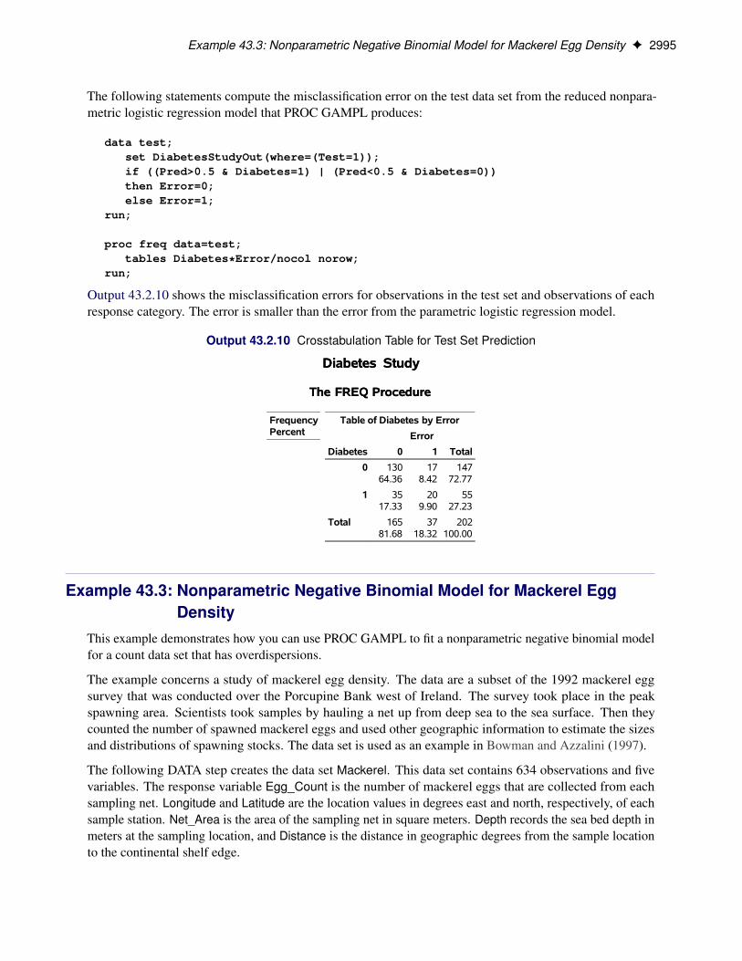
Example 43.3: Nonparametric Negative Binomial Model for Mackerel Egg Density F 2995
The following statements compute the misclassification error on the test data set from the reduced nonpara-metric logistic regression model that PROC GAMPL produces:
data test;set DiabetesStudyOut(where=(Test=1));if ((Pred>0.5 & Diabetes=1) | (Pred<0.5 & Diabetes=0))then Error=0;else Error=1;
run;
proc freq data=test;tables Diabetes*Error/nocol norow;
run;
Output 43.2.10 shows the misclassification errors for observations in the test set and observations of eachresponse category. The error is smaller than the error from the parametric logistic regression model.
Output 43.2.10 Crosstabulation Table for Test Set Prediction
Diabetes Study
The FREQ Procedure
Diabetes Study
The FREQ Procedure
FrequencyPercent
Table of Diabetes by Error
Diabetes
Error
0 1 Total
0 13064.36
178.42
14772.77
1 3517.33
209.90
5527.23
Total 16581.68
3718.32
202100.00
Example 43.3: Nonparametric Negative Binomial Model for Mackerel EggDensity
This example demonstrates how you can use PROC GAMPL to fit a nonparametric negative binomial modelfor a count data set that has overdispersions.
The example concerns a study of mackerel egg density. The data are a subset of the 1992 mackerel eggsurvey that was conducted over the Porcupine Bank west of Ireland. The survey took place in the peakspawning area. Scientists took samples by hauling a net up from deep sea to the sea surface. Then theycounted the number of spawned mackerel eggs and used other geographic information to estimate the sizesand distributions of spawning stocks. The data set is used as an example in Bowman and Azzalini (1997).
The following DATA step creates the data set Mackerel. This data set contains 634 observations and fivevariables. The response variable Egg_Count is the number of mackerel eggs that are collected from eachsampling net. Longitude and Latitude are the location values in degrees east and north, respectively, of eachsample station. Net_Area is the area of the sampling net in square meters. Depth records the sea bed depth inmeters at the sampling location, and Distance is the distance in geographic degrees from the sample locationto the continental shelf edge.

2996 F Chapter 43: The GAMPL Procedure
title 'Mackerel Egg Density Study';data Mackerel;
input Egg_Count Longitude Latitude Net_Area Depth Distance;datalines;0 -4.65 44.57 0.242 4342 0.83951411770 -4.48 44.57 0.242 4334 0.85919263360 -4.3 44.57 0.242 4286 0.89301528951 -2.87 44.02 0.242 1438 0.39564086914 -2.07 44.02 0.242 166 0.04000882373 -2.13 44.02 0.242 460 0.09742344630 -2.27 44.02 0.242 810 0.2362566569
... more lines ...
22 -4.22 46.25 0.19 205 0.118112082821 -4.28 46.25 0.19 237 0.1299908540 -4.73 46.25 0.19 2500 0.33465005365 -4.25 47.23 0.19 114 0.7181925823 -3.72 47.25 0.19 100 0.99446697780 -3.25 47.25 0.19 64 1.2639918431
;
The response values are counts, so the Poisson distribution might be a reasonable model. The statistic ofinterest is the mackerel egg density, which can be formed as
Density D E.Count/=Net_Area
This is equivalent to a Poisson regression that uses the response variable Egg_Count, an offset variablelog.Net_Area/, and other covariates.
The following statements produce the plot of the mackerel egg density with respect to the sampling stationlocation:
data Temp;set Mackerel;Density = Egg_Count/Net_Area;
run;
%let off0 = offsetmin=0 offsetmax=0linearopts=(thresholdmin=0 thresholdmax=0);
%let off0 = xaxisopts=(&off0) yaxisopts=(&off0);proc template;
define statgraph surface;dynamic _title _z;begingraph / designwidth=defaultDesignHeight;
entrytitle _title;layout overlay / &off0;
contourplotparm z=_z y=Latitude x=Longitude / gridded=FALSE;endlayout;
endgraph;end;
run;
proc sgrender data=Temp template=surface;dynamic _title='Mackerel Egg Density' _z='Density';
run;
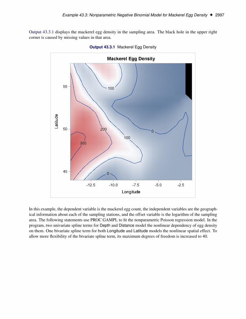
Example 43.3: Nonparametric Negative Binomial Model for Mackerel Egg Density F 2997
Output 43.3.1 displays the mackerel egg density in the sampling area. The black hole in the upper rightcorner is caused by missing values in that area.
Output 43.3.1 Mackerel Egg Density
In this example, the dependent variable is the mackerel egg count, the independent variables are the geograph-ical information about each of the sampling stations, and the offset variable is the logarithm of the samplingarea. The following statements use PROC GAMPL to fit the nonparametric Poisson regression model. In theprogram, two univariate spline terms for Depth and Distance model the nonlinear dependency of egg densityon them. One bivariate spline term for both Longitude and Latitude models the nonlinear spatial effect. Toallow more flexibility of the bivariate spline term, its maximum degrees of freedom is increased to 40.

2998 F Chapter 43: The GAMPL Procedure
data Mackerel;set Mackerel;Log_Net_Area = log(Net_Area);
run;
proc gampl data=Mackerel plots seed=2345;model Egg_Count = spline(Depth) spline(Distance)
spline(Longitude Latitude/maxdf=40)/ offset=Log_Net_Area dist=poisson;
output out=MackerelOut1 pred=Pred1 pearson=Pea1;run;
Output 43.3.2 displays the summary statistics from the Poisson model.
Output 43.3.2 Fit Statistics
Mackerel Egg Density Study
The GAMPL Procedure
Mackerel Egg Density Study
The GAMPL Procedure
Fit Statistics
Penalized Log Likelihood -2704.30290
Roughness Penalty 14.45972
Effective Degrees of Freedom 54.18388
Effective Degrees of Freedom for Error 578.23245
AIC (smaller is better) 5502.51384
AICC (smaller is better) 5512.84553
BIC (smaller is better) 5743.74311
UBRE (smaller is better) 6.58984
The “Tests for Smoothing Components” table in Output 43.3.3 shows that all spline terms are significant.
Output 43.3.3 Tests for Smoothing Components
Tests for Smoothing Components
ComponentEffective
DFEffective
DF for Test Chi-Square Pr > ChiSq
Spline(Depth) 8.00000 8 243.0414 <.0001
Spline(Distance) 7.95793 9 171.1765 <.0001
Spline(Longitude Latitude) 37.22594 39 4466.2848 <.0001
The smoothing component panel in Output 43.3.4 contains a contour for the spatial effect by Longitude andLatitude and two fitted univariate splines for Depth and Latitude, all demonstrating significantly nonlinearstructures.
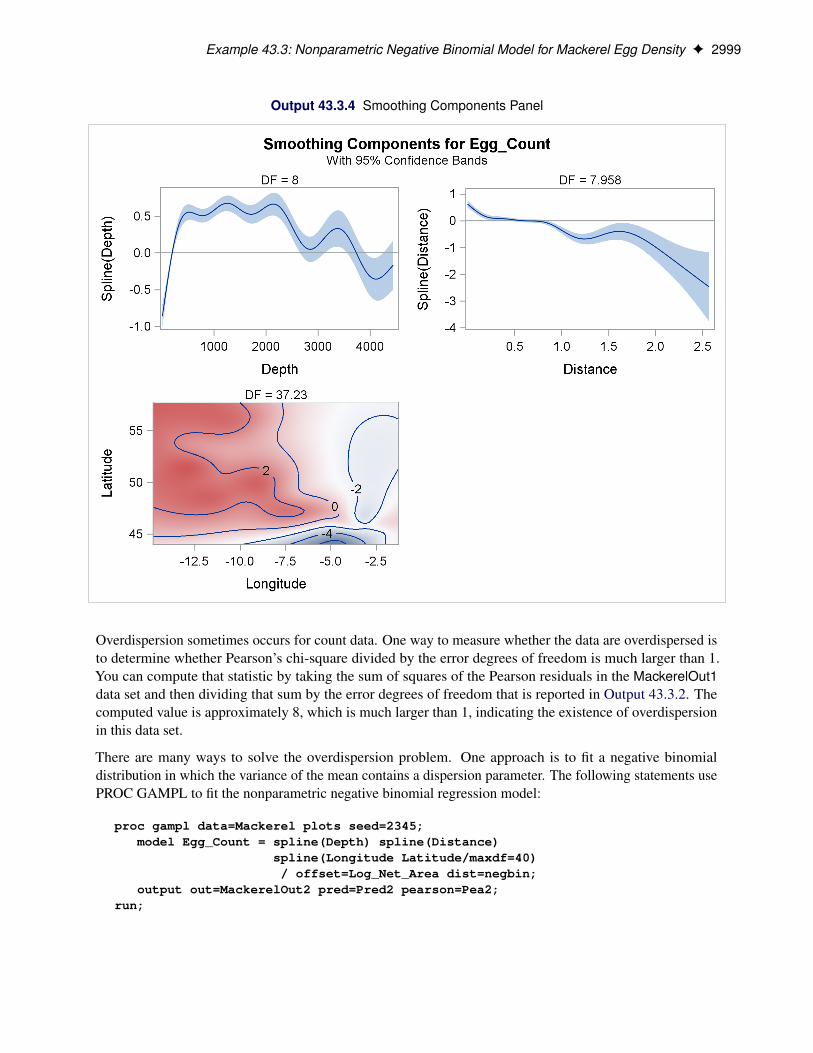
Example 43.3: Nonparametric Negative Binomial Model for Mackerel Egg Density F 2999
Output 43.3.4 Smoothing Components Panel
Overdispersion sometimes occurs for count data. One way to measure whether the data are overdispersed isto determine whether Pearson’s chi-square divided by the error degrees of freedom is much larger than 1.You can compute that statistic by taking the sum of squares of the Pearson residuals in the MackerelOut1data set and then dividing that sum by the error degrees of freedom that is reported in Output 43.3.2. Thecomputed value is approximately 8, which is much larger than 1, indicating the existence of overdispersionin this data set.
There are many ways to solve the overdispersion problem. One approach is to fit a negative binomialdistribution in which the variance of the mean contains a dispersion parameter. The following statements usePROC GAMPL to fit the nonparametric negative binomial regression model:
proc gampl data=Mackerel plots seed=2345;model Egg_Count = spline(Depth) spline(Distance)
spline(Longitude Latitude/maxdf=40)/ offset=Log_Net_Area dist=negbin;
output out=MackerelOut2 pred=Pred2 pearson=Pea2;run;

3000 F Chapter 43: The GAMPL Procedure
Output 43.3.5 displays the summary statistics from the negative binomial model. The model’s effectivedegrees of freedom is less than that of the Poisson model, even though the dispersion parameter costs oneextra degree of freedom to fit. The values of the information criteria are also much less, indicating a better fit.
Output 43.3.5 Fit Statistics
Mackerel Egg Density Study
The GAMPL Procedure
Mackerel Egg Density Study
The GAMPL Procedure
Fit Statistics
Penalized Log Likelihood -1559.27838
Roughness Penalty 17.31664
Effective Degrees of Freedom 43.04281
Effective Degrees of Freedom for Error 586.85164
AIC (smaller is better) 3187.32573
AICC (smaller is better) 3193.75239
BIC (smaller is better) 3378.95442
UBRE (smaller is better) 0.55834
The “Tests for Smoothing Components” table in Output 43.3.6 shows that all spline terms are significant.
Output 43.3.6 Tests for Smoothing Components
Tests for Smoothing Components
ComponentEffective
DFEffective
DF for Test F Value Pr > F
Spline(Depth) 8.00000 8 41.21 <.0001
Spline(Distance) 1.00010 1 8.33 0.0040
Spline(Longitude Latitude) 32.04271 37 1024.38 <.0001
The smoothing component panel in Output 43.3.7 contains a fitted surface and curves for the three splineterms. Compared to the Poisson model, the fitted surface and curves are smoother. It is possible thatthe nonlinear dependency structure becomes smoother after its partial variations are accounted for by thedispersion parameter.

Example 43.3: Nonparametric Negative Binomial Model for Mackerel Egg Density F 3001
Output 43.3.7 Smoothing Components Panel
Pearson’s chi-square divided by the error degrees of freedom for the negative binomial model is approximately1.5, which is close to 1. This suggests that the negative binomial model explains the overdispersion in thedata.
The following DATA step and statements visualize the contours of mackerel egg density for both Poisson andnegative binomial models:
data SurfaceFit;set Mackerel(keep=Longitude Latitude Net_Area Egg_Count);set MackerelOut1(keep=Pred1);set MackerelOut2(keep=Pred2);Pred1 = Pred1 / Net_Area;Pred2 = Pred2 / Net_Area;
run;
%let eopt = location=outside valign=top textattrs=graphlabeltext;proc template;
define statgraph surfaces;begingraph / designheight=360px;
layout lattice / columns=2;layout overlay / &off0;

3002 F Chapter 43: The GAMPL Procedure
entry "Poisson Model" / &eopt;contourplotparm z=Pred1 y=Latitude x=Longitude /
gridded=FALSE;endlayout;layout overlay / &off0;
entry "Negative Binomial Model" / &eopt;contourplotparm z=Pred2 y=Latitude x=Longitude /
gridded=FALSE;endlayout;
endlayout;endgraph;
end;run;
proc sgrender data=SurfaceFit template=surfaces;run;
Output 43.3.8 displays two fitted surfaces from the Poisson model and the negative binomial model, respec-tively.
Output 43.3.8 Fitted Surfaces from Poisson Model and Negative Binomial Model

References F 3003
References
Bowman, A. W., and Azzalini, A. (1997). Applied Smoothing Techniques for Data Analysis. New York:Oxford University Press.
Craven, P., and Wahba, G. (1979). “Smoothing Noisy Data with Spline Functions.” Numerical Mathematics31:377–403.
Dennis, J. E., Gay, D. M., and Welsch, R. E. (1981). “An Adaptive Nonlinear Least-Squares Algorithm.”ACM Transactions on Mathematical Software 7:348–368.
Dennis, J. E., and Mei, H. H. W. (1979). “Two New Unconstrained Optimization Algorithms Which UseFunction and Gradient Values.” Journal of Optimization Theory and Applications 28:453–482.
Duchon, J. (1976). “Fonctions-spline et espérances conditionnelles de champs gaussiens.” Annales scien-tifiques de l’Université de Clermont-Ferrand 2, Série Mathématique 14:19–27.
Duchon, J. (1977). “Splines Minimizing Rotation-Invariant Semi-norms in Sobolev Spaces.” In ConstructiveTheory of Functions of Several Variables, edited by W. Schempp and K. Zeller, 85–100. New York:Springer-Verlag.
Eskow, E., and Schnabel, R. B. (1991). “Algorithm 695: Software for a New Modified Cholesky Factorization.”ACM Transactions on Mathematical Software 17:306–312.
Fletcher, R. (1987). Practical Methods of Optimization. 2nd ed. Chichester, UK: John Wiley & Sons.
Gay, D. M. (1983). “Subroutines for Unconstrained Minimization.” ACM Transactions on MathematicalSoftware 9:503–524.
Gu, C., and Wahba, G. (1991). “Minimizing GCV/GML Scores with Multiple Smoothing Parameters via theNewton Method.” SIAM Journal on Scientific Computing 12:383–398.
Lichman, M. (2013). “UCI Machine Learning Repository.” School of Information and Computer Sciences,University of California, Irvine. http://archive.ics.uci.edu/ml.
Moré, J. J., and Sorensen, D. C. (1983). “Computing a Trust-Region Step.” SIAM Journal on Scientific andStatistical Computing 4:553–572.
Nelder, J. A., and Wedderburn, R. W. M. (1972). “Generalized Linear Models.” Journal of the RoyalStatistical Society, Series A 135:370–384.
Nychka, D. (1988). “Bayesian Confidence Intervals for Smoothing Splines.” Journal of the AmericanStatistical Association 83:1134–1143.
Pace, R. K., and Barry, R. (1997). “Quick Computation of Spatial Autoregressive Estimators.” GeographicalAnalysis 29:232–247.
Ruppert, D., Wand, M. P., and Carroll, R. J. (2003). Semiparametric Regression. Cambridge: CambridgeUniversity Press.
Vlachos, P. (1998). “StatLib—Datasets Archive.” http://lib.stat.cmu.edu/datasets/.

3004 F Chapter 43: The GAMPL Procedure
Wahba, G. (1983). “Bayesian ‘Confidence Intervals’ for the Cross Validated Smoothing Spline.” Journal ofthe Royal Statistical Society, Series B 45:133–150.
Wood, S. (2003). “Thin Plate Regression Splines.” Journal of the Royal Statistical Society, Series B65:95–114.
Wood, S. (2004). “Stable and Efficient Multiple Smoothing Parameter Estimation for Generalized AdditiveModels.” Journal of the American Statistical Association 99:673–686.
Wood, S. (2006). Generalized Additive Models. Boca Raton, FL: Chapman & Hall/CRC.
Wood, S. (2008). “Fast Stable Direct Fitting and Smoothness Selection for Generalized Additive Models.”Journal of the Royal Statistical Society, Series B 70:495–518.
Wood, S. (2011). “Fast Stable Restricted Maximum Likelihood and Marginal Likelihood Estimation ofSemiparametric Generalized Linear Models.” Journal of the Royal Statistical Society, Series B 73:3–36.
Wood, S. (2012). “On p-Values for Smooth Components of an Extended Generalized AdditiveModel.” Biometrika 1–8. http://biomet.oxfordjournals.org/content/early/2012/10/18/biomet.ass048.abstract.
Xiang, D., and Wahba, G. (1996). “A Generalized Approximate Cross Validation for Smoothing Splines withNon-Gaussian Data.” Statistica Sinica 6:675–692.
Subject Index
class levelGAMPL procedure, 2949, 2980
computational methodGAMPL procedure, 2974
convergence criterionGAMPL procedure, 2948, 2951, 2952
convergence statusGAMPL procedure, 2981
data access informationGAMPL procedure, 2979
degrees of freedomGAMPL procedure, 2972
dispersion parameterGAMPL procedure, 2973
displayed outputGAMPL procedure, 2979
distribution functionGAMPL procedure, 2960
effectname length (GAMPL), 2948
estimates for smoothing componentsGAMPL procedure, 2981
fit statisticsGAMPL procedure, 2981
fitting algorithmsGAMPL procedure, 2970
frequency variableGAMPL procedure, 2954
GAMPL procedure, 2937class level, 2949, 2980computational method, 2974convergence criterion, 2948, 2951, 2952convergence status, 2981data access information, 2979degrees of freedom, 2972dispersion parameter, 2973displayed output, 2979distribution function, 2960effect name length, 2948estimates for smoothing components, 2981fit statistics, 2981fitting algorithms, 2970function-based convergence criteria, 2951generalized additive models, 2967generalized linear models, 2967
gradient-based convergence criteria, 2951, 2952input data sets, 2948iteration history, 2980link function, 2961low-rank approximation, 2966model evaluation criteria, 2969model inference, 2973model information, 2979model options summary, 2955multithreading, 2964, 2974number of observations, 2980ODS Graphics, 2983ODS table names, 2982optimization technique, 2975outer iteration, 2971parameter estimates, 2981penalized likelihood estimation, 2969performance information, 2979performance iteration, 2971response level ordering, 2956response profile, 2980response variable options, 2956spline details, 2980tests for smoothing components, 2974, 2982thin-plate regression splines, 2965thin-plate smoothing splines, 2965user-defined formats, 2948weighting, 2965XML input stream, 2948
generalized additive modelsGAMPL procedure, 2967
generalized linear modelsGAMPL procedure, 2967
iteration historyGAMPL procedure, 2980
link functionGAMPL procedure, 2961
low-rank approximationGAMPL procedure, 2966
model evaluation criteriaGAMPL procedure, 2969
model inferenceGAMPL procedure, 2973
model informationGAMPL procedure, 2979
multithreading
GAMPL procedure, 2964, 2974
number of observationsGAMPL procedure, 2980
ODS GraphicsGAMPL procedure, 2983
ODS table namesGAMPL procedure, 2982
optimization techniqueGAMPL procedure, 2975
options summaryPROC GAMPL statement, 2947
outer iterationGAMPL procedure, 2971
parameter estimatesGAMPL procedure, 2981
penalized likelihood estimationGAMPL procedure, 2969
performance informationGAMPL procedure, 2979
performance iterationGAMPL procedure, 2971
response level orderingGAMPL procedure, 2956
response profileGAMPL procedure, 2980
response variable optionsGAMPL procedure, 2956
reverse response level orderingGAMPL procedure, 2956
spline detailsGAMPL procedure, 2980
tests for smoothing componentsGAMPL procedure, 2974, 2982
thin-plate regression splinesGAMPL procedure, 2965
thin-plate smoothing splinesGAMPL procedure, 2965
weightingGAMPL procedure, 2965
Syntax Index
ABSCONV optionPROC GAMPL statement, 2951
ABSFCONV optionPROC GAMPL statement, 2951
ABSGCONV optionPROC GAMPL statement, 2951
ABSGTOL optionPROC GAMPL statement, 2951
ABSTOL optionPROC GAMPL statement, 2951
ALLOBS optionMODEL statement (GAMPL), 2960
ALPHA= optionOUTPUT statement (GAMPL), 2964PROC GAMPL statement, 2948
CLASS statementGAMPL procedure, 2953
COMPONENT optionOUTPUT statement (GAMPL), 2964
CRITERION= optionMODEL statement (GAMPL), 2960
DATA= optionOUTPUT statement (GAMPL), 2963PROC GAMPL statement, 2948
DESCENDING optionMODEL statement (GAMPL), 2956
DETAILS optionMODEL statement (GAMPL), 2958
DF= optionMODEL statement (GAMPL), 2958
DISPERSION= optionMODEL statement (GAMPL), 2960
DISTRIBUTION= optionMODEL statement (GAMPL), 2960
FCONV optionPROC GAMPL statement, 2951
FDHESSIAN= optionMODEL statement (GAMPL), 2961
FMTLIBXML= optionPROC GAMPL statement, 2948
FREQ statementGAMPL procedure, 2954
FTOL optionPROC GAMPL statement, 2951
GAMPL procedure, 2947
CLASS statement, 2953FREQ statement, 2954ID statement, 2954MODEL statement, 2954OUTPUT statement, 2963PERFORMANCE statement, 2964PROC GAMPL statement, 2947syntax, 2947WEIGHT statement, 2965
GAMPL procedure, CLASS statement, 2953GAMPL procedure, FREQ statement, 2954GAMPL procedure, ID statement, 2954GAMPL procedure, MODEL statement, 2954
ALLOBS option, 2960CRITERION= option, 2960DESCENDING option, 2956DETAILS option, 2958DF= option, 2958DISPERSION= option, 2960DISTRIBUTION= option, 2960FDHESSIAN option, 2961INITIALPHI= option, 2961INITSMOOTH= option, 2958KNOTS= option, 2958LINK= option, 2961M= option, 2959MAXDF= option, 2959MAXKNOTS= option, 2959MAXPHI= option, 2962MAXSMOOTH= option, 2959METHOD= option, 2962MINPHI= option, 2962MINSMOOTH= option, 2960NORMALIZE option, 2962OFFSET= option, 2962ORDER= option, 2957RIDGE= option, 2963SCALE= option, 2963SMOOTH= option, 2960
GAMPL procedure, OUTPUT statement, 2963ALPHA= option, 2964COMPONENT option, 2964DATA= option, 2963keyword= option, 2963OUT= option, 2963
GAMPL procedure, PERFORMANCE statement,2964
GAMPL procedure, PROC GAMPL statement, 2947

ABSCONV option, 2951ABSFCONV option, 2951ABSFTOL option, 2951ABSGCONV option, 2951ABSGTOL option, 2951ABSTOL option, 2951ALPHA= option, 2948DATA= option, 2948FCONV option, 2951FMTLIBXML= option, 2948FTOL option, 2951GCONV option, 2952GTOL option, 2952ITDETAILS option, 2948MAXFUNC= option, 2952MAXITER= option, 2952, 2953MAXTIME= option, 2953NAMELEN= option, 2948NOCLPRINT option, 2949NOPRINT option, 2949PLIKEOPTIONS option, 2949plots(unpack) option, 2949PLOTS= option, 2949SEED= option, 2950SINGCHOL= option, 2950SINGSWEEP= option, 2950SINGULAR= option, 2950SMOOTHOPTIONS option, 2950TECHNIQUE= option, 2953
GAMPL procedure, WEIGHT statement, 2965GCONV option
PROC GAMPL statement, 2952GTOL option
PROC GAMPL statement, 2952
ID statementGAMPL procedure, 2954
INITIALPHI= optionMODEL statement (GAMPL), 2961
INITSMOOTH= optionMODEL statement (GAMPL), 2958
ITDETAILS optionPROC GAMPL statement, 2948
keyword= optionOUTPUT statement (GAMPL), 2963
KNOTS= optionMODEL statement (GAMPL), 2958
LINK= optionMODEL statement (GAMPL), 2961
M= optionMODEL statement (GAMPL), 2959
MAXDF= option
MODEL statement (GAMPL), 2959MAXFUNC= option
PROC GAMPL statement, 2952MAXITER= option
PROC GAMPL statement, 2952, 2953MAXKNOTS= option
MODEL statement (GAMPL), 2959MAXPHI= option
MODEL statement (GAMPL), 2962MAXSMOOTH= option
MODEL statement (GAMPL), 2959MAXTIME= option
PROC GAMPL statement, 2953METHOD= option
MODEL statement (GAMPL), 2962MINPHI= option
MODEL statement (GAMPL), 2962MINSMOOTH= option
MODEL statement (GAMPL), 2960MODEL statement
GAMPL procedure, 2954
NAMELEN= optionPROC GAMPL statement, 2948
NOCLPRINT optionPROC GAMPL statement, 2949
NOPRINT optionPROC GAMPL statement, 2949
NORMALIZE optionMODEL statement (GAMPL), 2962
OFFSET= optionMODEL statement (GAMPL), 2962
ORDER= optionMODEL statement (GAMPL), 2957
OUT= optionOUTPUT statement (GAMPL), 2963
OUTPUT statementGAMPL procedure, 2963
PERFORMANCE statementGAMPL procedure, 2964
PLIKEOPTIONS optionPROC GAMPL statement, 2949
PLOTS= optionPROC GAMPL statement, 2949
PROC GAMPL statement, see GAMPL procedure
RIDGE= optionMODEL statement (GAMPL), 2963
SCALE= optionMODEL statement (GAMPL), 2963
SEED= optionPROC GAMPL statement, 2950

SINGCHOL= optionPROC GAMPL statement, 2950
SINGSWEEP= optionPROC GAMPL statement, 2950
SINGULAR= optionPROC GAMPL statement, 2950
SMOOTH= optionMODEL statement (GAMPL), 2960
SMOOTHOPTIONS optionPROC GAMPL statement, 2950
syntaxGAMPL procedure, 2947
TECHNIQUE= optionPROC GAMPL statement, 2953
unpack optionPROC GAMPL statement, 2949
WEIGHT statementGAMPL procedure, 2965