The Fundamental Surplus

Lars Ljungqvist Thomas J. Sargent∗

June 10, 2016

Abstract

To generate big responses of unemployment to productivity changes, researchers have

reconfigured matching models in various ways: by elevating the utility of leisure, by

making wages sticky, by assuming alternating-offer wage bargaining, by introducing

costly acquisition of credit, by assuming fixed matching costs, or by positing govern-

ment mandated unemployment compensation and layoff costs. All of these redesigned

matching models increase responses of unemployment to movements in productivity by

diminishing the fundamental surplus fraction, an upper bound on the fraction of a job’s

output that the invisible hand can allocate to vacancy creation. Business cycles and

welfare state dynamics of an entire class of reconfigured matching models all operate

through this common channel.

Key words: Matching model, market tightness, fundamental surplus, unemployment,

volatility, business cycle, welfare state.

∗Ljungqvist: Stockholm School of Economics and New York University (email: lars.ljungqvist@hhs.se);Sargent: New York University and Hoover Institution (email: thomas.sargent@nyu.edu). We are grateful forexcellent research assistance by Isaac Baley, Cecilia Parlatore Siritto, and Jesse Perla. For their commentson earlier drafts we thank participants at the conference on Recursive Methods in Economic Dynamics, inHonor of 25 Years of [the treatise by] Stokey, Lucas, and Prescott, hosted by the Federal Reserve Bank ofMinneapolis, participants at the European Summer Symposium in International Macroeconomics (ESSIM)2015, and also Ross Doppelt, John Leahy, and Eran Yashiv. We thank Nicolas Petrosky-Nadeau and EtienneWasmer for inspiring us to add section 5.4, and Lawrence Christiano, Martin Eichenbaum and MathiasTrabandt for conducting the experiment in section 8.2. Ljungqvist’s research was supported by a grant fromthe Jan Wallander and Tom Hedelius Foundation.

1

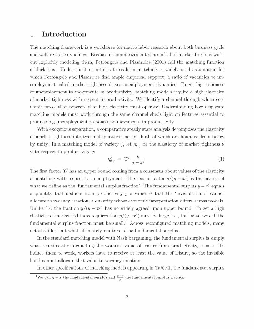
1 Introduction

The matching framework is a workhorse for macro labor research about both business cycle

and welfare state dynamics. Because it summarizes outcomes of labor market frictions with-

out explicitly modeling them, Petrongolo and Pissarides (2001) call the matching function

a black box. Under constant returns to scale in matching, a widely used assumption for

which Petrongolo and Pissarides find ample empirical support, a ratio of vacancies to un-

employment called market tightness drives unemployment dynamics. To get big responses

of unemployment to movements in productivity, matching models require a high elasticity

of market tightness with respect to productivity. We identify a channel through which eco-

nomic forces that generate that high elasticity must operate. Understanding how disparate

matching models must work through the same channel sheds light on features essential to

produce big unemployment responses to movements in productivity.

With exogenous separation, a comparative steady state analysis decomposes the elasticity

of market tightness into two multiplicative factors, both of which are bounded from below

by unity. In a matching model of variety j, let ηjθ,y be the elasticity of market tightness θ

with respect to productivity y:

ηjθ,y = Υj y

y − xj. (1)

The first factor Υj has an upper bound coming from a consensus about values of the elasticity

of matching with respect to unemployment. The second factor y/(y − xj) is the inverse of

what we define as the ‘fundamental surplus fraction’. The fundamental surplus y−xj equals

a quantity that deducts from productivity y a value xj that the ‘invisible hand’ cannot

allocate to vacancy creation, a quantity whose economic interpretation differs across models.

Unlike Υj , the fraction y/(y − xj) has no widely agreed upon upper bound. To get a high

elasticity of market tightness requires that y/(y−xj) must be large, i.e., that what we call the

fundamental surplus fraction must be small.1 Across reconfigured matching models, many

details differ, but what ultimately matters is the fundamental surplus.

In the standard matching model with Nash bargaining, the fundamental surplus is simply

what remains after deducting the worker’s value of leisure from productivity, x = z. To

induce them to work, workers have to receive at least the value of leisure, so the invisible

hand cannot allocate that value to vacancy creation.

In other specifications of matching models appearing in Table 1, the fundamental surplus

1We call y − x the fundamental surplus and y−xy the fundamental surplus fraction.

2

Table 1: Elasticities of market tightness and fundamental surpluses

Business cycle context Elasticity Key variables

Nash bargainingΥNash y

y − zz, value of leisure

(Hagedorn and Manovskii 2008)Sticky wage Υsticky y

y − ww, sticky wage

(Hall 2005). . . and a financial accelerator Υsticky y

y − w − kk, annuitized value of

(Wasmer and Weil 2004) credit search costsAlternating-offer bargaining Υsticky y

y − z − β(1− s)γγ, firm’s cost of delay

(Hall and Milgrom 2008) in bargaining �

Fixed matching cost ΥNash yy − z − β(r + s)H

H , fixed matching(Pissarides 2009) cost �

Welfare state context †

Unemployment insurance ΥNash yy − z − b

b, unemploymentbenefit

Layoff costs ΥNash yy − z − βsτ

τ , layoff tax �

� Other parameters are the discount factor β = (1 + r)−1, and the separation rate s.† Theories that attribute high European unemployment to productivity changes include a widened

earnings distribution in Mortensen and Pissarides (1999), higher capital-embodied technological

change in Hornstein et al. (2007), and shocks to human capital in Ljungqvist and Sargent (2007).

emerges after making other deductions from productivity. In a model with a sticky wage

w, the deduction is simply the wage itself, x = w, since the invisible hand cannot allocate

so much to vacancy creation that there remains too little to pay the wage. If there is also

costly acquisition of credit, as in Wasmer and Weil’s (2004) model of a financial accelerator,

an additional deduction needed to arrive at the fundamental surplus is the annuitized value

k of the average search costs for the formation of a unit that can post a vacancy, so here

x = w+k. Similarly, in the case of a layoff tax τ for which liability arises after the formation

of an employment relationship, the fundamental surplus under Nash bargaining is obtained

by deducting the value of leisure and also a value reflecting the eventual payment of the layoff

tax, x = z + βsτ , where the product of the discount factor β, match destruction probability

s, and the layoff tax τ is an annuity payment that has the same expected present value as

the layoff tax. In Hall and Milgrom’s (2008) model of alternating-offer wage bargaining, we

must deduct both the value of leisure and a quantity measuring a worker’s ability to impose

3

a cost of delay γ on the firm. When firms make the first wage offer, the fundamental surplus

is obtained by making deduction x = z + β(1 − s)γ (when it is assumed that a bargaining

firm-worker pair faces the same separation rate s before and after an agreement is reached).

This paper finds (1) that as a fraction of productivity, the fundamental surplus must be

small to produce high unemployment volatility during business cycles, and (2) that a small

fundamental surplus fraction also explains high unemployment coming from adverse welfare

state incentives. Within several matching models, we dissect the forces at work by presenting

closed-form solutions for steady-state comparative statics, and also by reporting numerical

simulations that confirm how those same forces also shape outcomes in stochastic models.

The following mechanical intuition underlies our findings. The fundamental surplus is an

upper bound on what the invisible hand can allocate to vacancy creation. A given change

in productivity translates into a larger percentage change in the fundamental surplus when

the fundamental surplus fraction is small. That induces the invisible hand to make resources

allocated to vacancy costs comove strongly with changes in productivity. The relationship

is immediate in a matching model with a sticky wage because a free-entry condition in

vacancy creation equates the expected cost of filling a vacancy to the expected present value

of the difference between a job’s productivity and the sticky wage. Consequently, a change in

productivity has a direct impact on resources devoted to vacancy creation. If those resources

are small relative to output, a given percentage change in productivity translates into a much

larger percentage change in resources used for vacancy creation and hence big responses of

unemployment to movements in productivity. The relationship is subtler but similar in other

matching models in which changes in productivity that have large effects on the fundamental

surplus must also affect the equilibrium amount of resources devoted to vacancy creation.

After setting forth a standard matching model in section 2, section 3 explains the role

of the fundamental surplus as an object uniting seemingly disparate matching models. We

derive steady-state comparative-statics expressions for the elasticity of market tightness with

respect to productivity in models of welfare states and business cycles in sections 4 and 5,

respectively. Section 6 discusses how the effects of the fundamental surplus are mediated

through the dynamics of wages and profits. Stochastic versions of business cycle models are

simulated in section 7. Section 8 demonstrates the usefulness of the fundamental surplus

in richer environments that embed matching models. Section 9 offers concluding remarks.

(Some computational details are relegated to an online appendix.)

We tell where important earlier accounts of the forces at work were incomplete or mislead-

ing. Rogerson and Shimer’s (2011) attribution of a low (high) elasticity of market tightness

4

to a high (low) elasticity of the wage with respect to productivity in Nash bargaining mod-

els identifies neither a necessary nor a sufficient condition. Hall’s (2005) sticky wage and

Hall and Milgrom’s (2008) use of special bargaining protocols to suppress a worker’s outside

value fail to imply a high elasticity of market tightness because they need not imply a small

fundamental surplus fraction. As astutely noted by Hagedorn and Manovskii (2008), a high

elasticity of market tightness requires that profits are small and elastic. We show that for

that to happen the fundamental surplus fraction must be small. Instead of stopping with

proximate causes cast in terms of endogenous outcomes (e.g., small and elastic profits), we

advocate focusing on primitives that determine the fundamental surplus. Failure to do in

earlier work has occasionally obscured ultimate causes. For example, a decomposition of

Petrosky-Nadeau and Wasmer (2013) assigns a multiplicative role to a financial accelerator

in the model of Wasmer and Weil (2004). We show that eliminating endogenous quantities

in favor of exogenous ones reveals how the fundamental surplus fraction in Table 1 is the

essential determinant. On a positive note, Mortensen and Nagypal (2007) combined several

forces in ways that are consistent with our argument that all components of productivity

that the ‘invisible hand’ cannot allocate to vacancy creation contribute to increasing the

elasticity of market tightness by diminishing the fundamental surplus fraction.

2 Preliminaries

To set the stage, we review key equations and equilibrium relationships for a basic discrete

time matching model.2 There is a continuum of identical workers with measure 1. Workers

are infinitely lived and risk neutral with discount factor β = (1 + r)−1. A worker wants

to maximize the expected discounted sum of labor income plus the value of leisure. An

employed worker gets labor income equal to the wage w and no leisure. An unemployed

worker receives value of leisure z > 0 and no labor income.

The production technology has constant returns to scale with labor as the sole input.

Each employed worker produces y units of output. Each firm employs at most one worker.

A firm incurs a vacancy cost c each period it waits to find a worker. While matched with a

worker, a firm’s per-period earnings are y − w. All matches are exogenously destroyed with

per-period probability s. Free entry implies that a new firm’s expected discounted stream of

vacancy costs plus earnings equals zero.

A matching function M(u, v) determines the measure of successful matches in a period,

2See Ljungqvist and Sargent (2012, section 28.3), or for a continuous time version, see Pissarides (2000).

5

where u and v are aggregate measures of unemployed workers and vacancies. The matching

function M is increasing in both arguments, concave, and homogeneous of degree 1. Homo-

geneity implies that the probability of filling a vacancy is q(v/u) ≡ M(u, v)/v. The ratio

θ ≡ v/u of vacancies to unemployed workers is called market tightness. The probability that

an unemployed worker will be matched in a period is θq(θ).

A firm’s values J of a filled job and V of a vacancy satisfy the Bellman equations

J = y − w + β [sV + (1− s)J ] , (2)

V = −c + β{q(θ)J + [1− q(θ)]V

}. (3)

After imposing the zero profit condition V = 0, equation (3) implies

J =c

βq(θ), (4)

which we can substitute into equation (2) to arrive at

w = y − r + s

q(θ)c . (5)

A worker’s values as employed E and as unemployed U satisfy the Bellman equations

E = w + β[sU + (1− s)E

], (6)

U = z + β{θq(θ)E + [1− θq(θ)]U

}. (7)

In the basic matching model, the match surplus S ≡ J + E − U is split between a

matched firm and worker according to Nash bargaining. The maximizers of Nash product

(E − U)φJ1−φ satisfy

E − U = φS and J = (1− φ)S , (8)

where φ ∈ [0, 1) measures the worker’s ‘bargaining power’. After solving equations (2) and

(6) for J and E, respectively, then substituting them into equations (8), we find that the

wage rate satisfies

w =r

1 + rU + φ

(y − r

1 + rU

). (9)

The annuity value of being unemployed, rU/(1+ r), can be obtained by solving equation (7)

6

for E − U and substituting this expression and equation (4) into equations (8):

r

1 + rU = z +

φ θ c

1− φ. (10)

Substituting equation (10) into equation (9) yields

w = z + φ(y − z + θc) . (11)

The two expressions (5) and (11) for the wage rate jointly determine the equilibrium

value of θ:

y − z =r + s + φ θ q(θ)

(1− φ)q(θ)c . (12)

The assumptions of identical workers/vacancies, risk neutrality, and constant returns to scale

in both production and matching imply that equilibrium market tightness θ does not depend

on composition of workers between those employed and those unemployed. In a steady state,

θ determines unemployment by the condition that the measure of workers laid off in a period,

s(1−u), must equal the measure of unemployed workers gaining employment, θq(θ)u, which

implies

u =s

s + θq(θ). (13)

We proceed under the assumption that the matching function has the Cobb-Douglas

form, M(u, v) = Auαv1−α, where A > 0, and α ∈ (0, 1) is the constant elasticity of matching

with respect to unemployment, α = −q′(θ) θ/q(θ).

3 Fundamental surplus as essential object

In equation (13), the derivative of steady-state unemployment with respect to market tight-

ness is

d u

d θ= −s [q(θ) + θ q′(θ)]

[s + θ q(θ)]2= −

[1 +

θ q′(θ)q(θ)

]u q(θ)

s + θ q(θ)= −(1− α)

u q(θ)

s + θ q(θ),

where the second equality uses equation (13) and factors q(θ) from the expression in square

brackets of the numerator, and the third equality is obtained after invoking the constant

elasticity of matching with respect to unemployment. So the elasticity of unemployment

7

with respect to market tightness is

ηu,θ = −(1− α)θ q(θ)

s + θ q(θ)= −(1 − α)

(1 − s

s + θ q(θ)

)= −(1− α) (1− u) , (14)

where the second equality is obtained after adding and subtracting s to the numerator, and

the last third equality invokes expression (13).

To shed light on what contributes to significant volatility in unemployment, we seek

forces that can make market tightness θ highly elastic with respect to productivity.

3.1 A decomposition of the elasticity of market tightness

After implicit differentiation of expression (12), we can compute the elasticity of market

tightness with respect to productivity as

ηθ,y =(r + s) + φ θ q(θ)

α(r + s) + φ θ q(θ)

y

y − z≡ ΥNash y

y − z. (15)

(See online appendix A.1.) This multiplicative decomposition of the elasticity of market

tightness is central to our analysis. Similar decompositions prevail in all of the reconfig-

ured matching models to be described below. The first factor ΥNash in expression (15), has

counterparts in other setups. A consensus about reasonable calibrations bounds its contri-

bution to the elasticity of market tightness. Hence, the magnitude of the elasticity of market

tightness depends mostly on the second factor in expression (15), i.e., the inverse of what in

section 1 we defined to be the fundamental surplus fraction.

Shimer’s (2005) critique is that for common calibrations of the standard matching model,

the elasticity of market tightness is too low to explain business cycle fluctuations. Shimer

noted that the average job finding rate θ q(θ) is large relative to the observed value of the

sum of the net interest rate and the separation rate (r+s). When combined with reasonable

parameter values for a worker’s bargaining power φ and the elasticity of matching with

respect to unemployment α, this implies that the first factor ΥNash in expression (15), is

close to its lower bound of unity. More generally, the first factor in (15) is bounded from

above by 1/α. Since reasonable values of the elasticity α confine the first factor, it is the

second factor y/(y− z) in expression (15) that is critical in generating movements in market

tightness. For values of leisure within a commonly assumed range well below productivity,

the second factor is not large enough to generate the observed high volatility of market

8

tightness. This is Shimer’s critique.

Shimer (2005, pp. 39-40) documented that comparisons of steady states described by

expression (15) provide a good approximation to average outcomes from simulations of an

economy subject to aggregate productivity shocks. We will derive some closed-form solutions

for steady states in other setups. These will shed light on the findings from stochastic

simulations to be reported in section 7.

3.2 Relationship to match surplus and outside values

The match surplus is the capitalized surplus accruing to a firm and a worker in the current

match. It is the difference between the present value of the match and the sum of the worker’s

outside value and the firm’s outside value. By rearranging equation (7) and imposing the

first Nash-bargaining outcome of equations (8), E −U = φS, the worker’s outside value can

be expressed as

U =z

1− β+

β

1− βθq(θ)φS =

z

1− β+ Ψm.surplus

u + Ψextrau , (16)

where the second equality decomposes U into three nonnegative parts: (1) the capitalized

value of choosing leisure in all future periods, z(1 − β)−1; (2) the sum of the discounted

values of the worker’s share of match surpluses in his or her as yet unformed future matches3

Ψm.surplusu =

r + s

r

θ q(θ)

r + s + θ q(θ)φS ; (17)

3Let Ψm.surplusn be the analogous capital value of an employed worker’s share of all match surpluses

over lifetime, including current employment. The capital values Ψm.surplusu and Ψm.surplus

n solve the Bellmanequations

Ψm.surplusu = 0 + β

{θq(θ)Ψm.surplus

n + [1− θq(θ)] Ψm.surplusu

},

Ψm.surplusn = ψ + β

{(1− s)Ψm.surplus

n + sΨm.surplusu

},

where ψ is an annuity that, when paid for the duration of a match, has the same expected present value asa worker’s share of the match surplus, E − U = φS:

∞∑t=0

βt(1 − s)tψ = φS =⇒ ψ = (r + s)βφS .

9

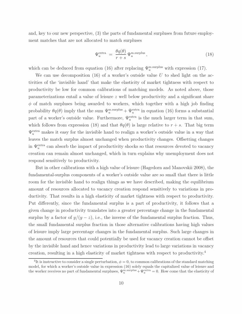
and, key to our new perspective, (3) the parts of fundamental surpluses from future employ-

ment matches that are not allocated to match surpluses

Ψextrau =

θq(θ)

r + sΨm.surplus

u , (18)

which can be deduced from equation (16) after replacing Ψm.surplusu with expression (17).

We can use decomposition (16) of a worker’s outside value U to shed light on the ac-

tivities of the ‘invisible hand’ that make the elasticity of market tightness with respect to

productivity be low for common calibrations of matching models. As noted above, those

parameterizations entail a value of leisure z well below productivity and a significant share

φ of match surpluses being awarded to workers, which together with a high job finding

probability θq(θ) imply that the sum Ψm.surplusu +Ψextra

u in equation (16) forms a substantial

part of a worker’s outside value. Furthermore, Ψextrau is the much larger term in that sum,

which follows from expression (18) and that θq(θ) is large relative to r + s. That big term

Ψextrau makes it easy for the invisible hand to realign a worker’s outside value in a way that

leaves the match surplus almost unchanged when productivity changes. Offsetting changes

in Ψextrau can absorb the impact of productivity shocks so that resources devoted to vacancy

creation can remain almost unchanged, which in turn explains why unemployment does not

respond sensitively to productivity.

But in other calibrations with a high value of leisure (Hagedorn and Manovskii 2008), the

fundamental-surplus components of a worker’s outside value are so small that there is little

room for the invisible hand to realign things as we have described, making the equilibrium

amount of resources allocated to vacancy creation respond sensitively to variations in pro-

ductivity. That results in a high elasticity of market tightness with respect to productivity.

Put differently, since the fundamental surplus is a part of productivity, it follows that a

given change in productivity translates into a greater percentage change in the fundamental

surplus by a factor of y/(y − z), i.e., the inverse of the fundamental surplus fraction. Thus,

the small fundamental surplus fraction in those alternative calibrations having high values

of leisure imply large percentage changes in the fundamental surplus. Such large changes in

the amount of resources that could potentially be used for vacancy creation cannot be offset

by the invisible hand and hence variations in productivity lead to large variations in vacancy

creation, resulting in a high elasticity of market tightness with respect to productivity.4

4It is instructive to consider a single perturbation, φ = 0, to common calibrations of the standard matchingmodel, for which a worker’s outside value in expression (16) solely equals the capitalized value of leisure andthe worker receives no part of fundamental surpluses, Ψm.surplus

u +Ψextrau = 0. How come that the elasticity of

10

Having described how the fundamental surplus supplements the concept of a worker’s

outside value, we now tell how the fundamental surplus relates to the match surplus. The

fundamental surplus is an upper bound on resources that the invisible hand can allocate

to vacancy creation. Its magnitude as a fraction of output is the prime determinant of

the elasticity of market tightness with respect to productivity.5 In contrast, although it is

directly connected to resources that are devoted to vacancy creation, a small size of the

match surplus relative to output has no direct bearing on the elasticity of market tightness.

Recall that in the standard matching model, the zero-profit condition for vacancy creation

implies that the expected present value of a firm’s share of match surpluses equals the average

cost of filling a vacancy. Since common calibrations award firms a significant share of match

surpluses, and since vacancy cost expenditures are calibrated to be relatively small, it follows

that equilibrium match surpluses must form small parts of output across various matching

models, regardless of the elasticity of market tightness in any particular model.

From an accounting perspective, match surpluses and firms’ profits emerge from fun-

damental surpluses. Hence, a small fundamental surplus fraction necessarily implies small

match surpluses and small firms’ profits. But, as we will show, the converse does not hold.

Small match surpluses and small firms’ profits need not imply small fundamental surpluses.

Therefore, the size of the fundamental surplus fraction is the only reliable indicator of the

magnitude of the elasticity of market tightness with respect to productivity, as conveyed by

expression (15).

Dynamics that are intermediated through the fundamental surplus occur in other pop-

ular setups, including those with sticky wages, alternative bargaining protocols and costly

acquisition of credit. For example, it matters little if the source of a diminished fundamental

surplus fraction is Hagedorn and Manovskii’s (2008) high value of leisure for workers, Hall’s

(2005) sticky wage, Hall and Milgrom’s (2008) cost of delay for firms that participate in

alternating-offer bargaining, or Wasmer and Weil’s (2004) upfront cost for firms to secure

credit. A small fundamental surplus fraction causes variations in productivity to have large

effects on resources devoted to vacancy creation either because workers insist on being com-

market tightness with respect to productivity remains low for such perturbed parameterizations where largefundamental surpluses only end up as firms’ profits which in an equilibrium are all used for vacancy creation?The answer lies precisely in the outcome that firms’ profits would then be truly large; therefore, even thoughvariations in productivity then affect firms’ profits directly, the percentage wise impact of productivity shockson such huge profits is negligible so market tightness and unemployment will hardly change. For furtherdiscussion of profits and fundamental surpluses, see section 6.

5We express the fundamental surplus as a flow value while the match surplus is typically a capitalizedvalue.

11

pensated for their losses of leisure, or because firms have to pay the sticky wage, or because

workers strategically exploit the firm’s cost of delay under an alternating-offer bargaining

protocol, or because firms must bear the cost of acquiring credit. Likewise, welfare state poli-

cies such as unemployment compensation and government-imposed layoff costs can reduce

the fundamental surplus fraction. We turn to welfare state policies next.

4 Fundamental surplus and welfare states

4.1 Unemployment compensation

We begin by considering a simplified version of Mortensen and Pissarides’ (1999) model of

workers who are heterogeneous in their skills and enjoy a welfare state safety net. Mortensen

and Pissarides make technological assumptions that imply that unemployed workers enter

skill-specific matching functions to match with vacancies at their skill levels. An important

assumption for Mortensen and Pissarides is that the value of leisure including unemploy-

ment compensation does not vary proportionately with workers’ skills. We incorporate these

features in our standard matching model by assuming that workers have different produc-

tivities y but a common value of leisure z, defined as a value that includes unemployment

compensation.

We set a value of leisure z = 0.6 and let workers’ productivities reside in the domain

[0.6, 1]. At the high-end of these productivities, z = .6 is a value of leisure within a range

typical of common calibrations of matching models. Following Mortensen and Pissarides

(1999), we assume that φ = α = 0.5, which is also a common calibration: workers’ bar-

gaining weight φ falls mid-range and equals the elasticity α of matching with respect to

unemployment, so that the Hosios efficiency condition is satisfied.

The model period is a day and the discount factor is β = 0.951/365, i.e., an annual

interest rate of 5 percent.6 A daily separation rate of s = 0.001 means that jobs last on

average 2.8 years. For the highest productivity level y = 1, we target an unemployment

rate of 5 percent, which by equation (13) implies that unemployed workers face a daily job

finding probability equal to θ q(θ) = 0.019, which means that the probability of finding a

job within a month is 44 percent. According to equilibrium expression (12), two parameters

6A short model period helps vacancy creation take place even at low values of the fundamental surplusfraction. Note that the lower bound on the average recruitment cost is attained when market tightness hasdropped so low that a vacancy encounters an unemployed worker with probability one, i.e., the recruitmentcost becomes certain and equals the one-period vacancy cost.

12

0.6 0.7 0.8 0.9 10

0.1

0.2

0.3

0.4

0.5

Rat

e

Productivity

Unemployment rate

Monthly job finding rate

0.6 0.7 0.8 0.9 10

0.1

0.2

0.3

0.4

0.5

Rec

ruitm

ent c

osts

as

a fr

actio

n of

fund

amen

tal s

urpl

us

Productivity

Equilibrium

Constant recruitment costs

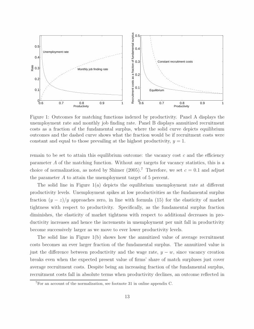
Figure 1: Outcomes for matching functions indexed by productivity. Panel A displays theunemployment rate and monthly job finding rate. Panel B displays annuitized recruitmentcosts as a fraction of the fundamental surplus, where the solid curve depicts equilibriumoutcomes and the dashed curve shows what the fraction would be if recruitment costs wereconstant and equal to those prevailing at the highest productivity, y = 1.

remain to be set to attain this equilibrium outcome: the vacancy cost c and the efficiency

parameter A of the matching function. Without any targets for vacancy statistics, this is a

choice of normalization, as noted by Shimer (2005).7 Therefore, we set c = 0.1 and adjust

the parameter A to attain the unemployment target of 5 percent.

The solid line in Figure 1(a) depicts the equilibrium unemployment rate at different

productivity levels. Unemployment spikes at low productivities as the fundamental surplus

fraction (y − z)/y approaches zero, in line with formula (15) for the elasticity of market

tightness with respect to productivity. Specifically, as the fundamental surplus fraction

diminishes, the elasticity of market tightness with respect to additional decreases in pro-

ductivity increases and hence the increments in unemployment per unit fall in productivity

become successively larger as we move to ever lower productivity levels.

The solid line in Figure 1(b) shows how the annuitized value of average recruitment

costs becomes an ever larger fraction of the fundamental surplus. The annuitized value is

just the difference between productivity and the wage rate, y − w, since vacancy creation

breaks even when the expected present value of firms’ share of match surpluses just cover

average recruitment costs. Despite being an increasing fraction of the fundamental surplus,

recruitment costs fall in absolute terms when productivity declines, an outcome reflected in

7For an account of the normalization, see footnote 31 in online appendix C.

13

the falling job finding probabilities in Figure 1(a). The dashed line in Figure 1(b) shows

the ratio of recruitment costs to the fundamental surplus required if these costs were to

have remained constant in absolute terms, and equal to those prevailing at the highest

productivity, y = 1.

Given our φ = 0.5 calibration (equal bargaining weights for workers and firms), the an-

nuitized match surplus as a fraction of the fundamental surplus is twice that of the solid

line in Figure 1(b), so it ranges from a mere 10 percent at high productivities to 100 percent

in the limit when productivity approaches the value of leisure. Hence, at the lower range

of productivities, recruitment costs are bound to fall with a drop in productivity. At low

productivity levels, the annuitized match surplus comprises almost the entire fundamental

surplus. Being unable to appropriate the value of a worker’s leisure, the “invisible hand”

has to let resources allocated to vacancy creation move with productivity. Together with

the fact that a given percentage change in productivity becomes so much larger as a per-

centage change of a small fundamental surplus (of which almost all is now allocated to the

match surplus), it follows that the elasticity of market tightness with respect to productivity

explodes as productivity approaches the value of leisure.

Mortensen and Pissarides (1999, p. 258) compare the unemployment schedule in Fig-

ure 1(a) to that for an economy with lower unemployment compensation parameterized as

a lower value of z – ‘Europe’ versus the ‘US’ – and conclude that “the relationship between

the unemployment rate and worker productivity is much more convex in the ‘European’ case

than in the ‘US’.” As we have shown, this outcome is a necessary consequence of a much

smaller fundamental surplus fraction in the economy with a higher value of z.

Next, Mortensen and Pissarides hypothesize that the widening unemployment difference

between Europe and the US after the late 1970s can be explained by ‘skill-biased’ technology

shocks, modeled as a mean preserving spread of the distribution of productivities across

workers. Figure 1(a) shows that moving workers to a lower range of productivities causes

a larger increase in unemployment than the decrease caused by moving workers to higher

productivities. Mortensen and Pissarides (1999, p. 259) add that such skill-biased shocks

“induce reductions in the participation rate like those observed in the major European

economies.” In our language, this occurs because the fundamental surplus becomes too

small or perhaps even negative, making vacancy creation shut down and market tightness

become zero in the matching functions for workers with low productivities.8

8Instead of assuming that individual workers are permanently attached to their productivity levels,Ljungqvist and Sargent (2007) formulate a matching model with skills that accumulate through work ex-

14

4.2 Layoff taxes

We assume that the government imposes a layoff tax τ on each layoff. Tax revenues are

returned as lump sum transfers to workers, but because they do not affect behavior, these

transfers do not appear in the expressions below. To promote transparency, we retain exoge-

nous job destruction and focus on how layoff taxes affect the elasticity of market tightness

with respect to productivity. We again find that the elasticity of market tightness with

respect to productivity depends on the size of the fundamental surplus fraction.

When liability for the layoff tax arises after the formation of an employment relationship,

Nash bargaining solution (8) continues to hold, i.e., a worker and a firm split match surpluses,

including a negative match surplus at a separation, S = −τ , according to their respective

bargaining powers

(1− φ)(E − U) = φJ . (19)

Hence, in the presence of a layoff tax, Bellman equations for the value J to a firm of a filled

job and the value E of an employed worker in expressions (2) and (6) become

J = y − w + β[−s(1− φ)τ + (1− s)J

](20)

E = w + β[s(U − φτ) + (1− s)E

], (21)

where we have imposed V = 0 so that vacancies break even in an equilibrium. The no-profit

condition for vacancies from expression (4) and the value of an unemployed worker from

expression (7) remain the same.

Paralleling the steps in section 2, we can derive two expressions that the equilibrium wage

must satisfy. (See online appendix A.2.) When equating those two expressions, we obtain

the following equation for equilibrium market tightness θ:

y − z − βsτ =r + s + φ θ q(θ)

(1− φ)q(θ)c . (22)

perience. They attribute high European unemployment to an increase in economic turbulence, modeled asskill loss at job separations, and to generous unemployment insurance that is paid as a fixed replacement ofa worker’s past earnings. If there are separate matching functions for all combinations of skill and benefitlevels, the counterpart in Ljungqvist and Sargent’s model to workers farthest to the left in Figure 1(a) wouldbe low-skilled, high-benefit unemployed workers, i.e., the lowest fundamental surplus fractions are associatedwith workers who have suffered skill loss and are now entitled to high benefits based on their past high earn-ings. Ljungqvist and Sargent also show how the adverse consequences of the presence of a set of low-skilled,high-benefit unemployed workers are diluted when these workers are assigned to matching functions withother workers associated with a larger fundamental surplus, e.g., if there is a single matching function forall unemployed workers.

15

After implicit differentiation, we can compute the elasticity of market tightness as

ηθ,y = ΥNash y

y − z − βsτ. (23)

The only difference between the elasticity of market tightness with a layoff tax (23) and the

earlier expression (15) without layoff taxes is that the fundamental surplus has an additional

deduction of βsτ . So long as the firm continues to operate, this is an annuity payment a

having the same expected present value as the layoff tax:

∞∑t=0

βt(1− s)ta =

∞∑t=1

βt(1− s)t−1s τ =⇒ a = βsτ , (24)

where the flow of annuity payments on the left side of the first equation starts in the first

period of operating and ceases when the job is destroyed, while the future layoff tax on the

right side occurs first after the initial period of operation. Since the “invisible hand” can

never allocate those resources to vacancy creation, it is appropriate to subtract this annuity

value when computing the fundamental surplus.

Some modelers have used the alternative assumption that firms are liable for the layoff

tax immediately upon being matched with unemployed workers regardless of whether em-

ployment relationships are eventually formed, e.g. see Millard and Mortensen (1997). Under

this assumption, online appendix A.3 derives the elasticity of market tightness as a two-

factor decomposition similar to expression (23). While details differ, the message remains

the same. Since the first factor of the decomposition is confined by a generally accepted

upper bound, a high elasticity of market tightness requires that the second factor be large,

i.e., that a properly defined fundamental surplus fraction be small.9

4.3 Fixed matching cost

In addition to a vacancy posting cost c per period, we now assume that a firm incurs a fixed

cost H when matching with a worker. It is instructive to compare outcomes to those from

9The first factor is bounded from above by max{α−1, (1 − α)−1}. The second factor involves the Nashbargaining shares, 1−φ and φ, for the following two reasons: (i) since the layoff tax must ex ante be financedout of the firm’s match surplus, the deduction from the fundamental surplus associated with the layoff tax isamplified by a smaller share 1−φ of the match surplus going to the firm; and (ii) because firms are liable forthe layoff tax after merely meeting unemployed workers, workers exploit that fact in bargaining. The latteritem (ii) brings an implicit interest cost, weighted by the worker’s bargaining power φ, to be deducted fromthe fundamental surplus as if the layoff tax had been incurred already at the beginning of the employmentrelationship. This resembles the upfront fixed matching cost in section 4.3.

16

layoff taxes.

If the firm incurs the cost H after bargaining with the worker (e.g., a training cost before

work commences), online appendix A.4 derives the elasticity of market tightness to be

ηθ,y = ΥNash y

y − z − β(r + s)H, (25)

which is almost identical to expression (23), which we derived for the case in which liability

for layoff taxes arises after the formation of employment relationships. The only difference

is that the fixed matching cost H is incurred at the start and the layoff tax τ at the end of

a match. Hence, the fundamental surplus under a fixed matching cost is further reduced by

an additional interest cost for the upfront expenditure, βrH .10

Beyond reaffirming Pissarides’s (2009) insight that the addition of a fixed matching cost

increases the elasticity of market tightness, our analysis thus adds the important refinement

that the quantitative importance of that fixed cost is inversely related to the ultimate size

of the fundamental surplus fraction.

5 Fundamental surplus and business cycles

5.1 Alternative calibration

To confront the Shimer critique, Hagedorn and Manovskii (2008) propose an alternative

calibration of a standard matching model that effectively places the economy at the left

end of our Figure 1(a). To illustrate, let the productivities 0.61, 0.63, and 0.65 in Figure

1(a) represent three different economies with homogeneous workers. For each economy, we

renormalize the efficiency parameter A in the matching function to make the unemployment

rate be 5 percent at the economy’s postulated productivity level. Figure 2 shows how the

steady-state unemployment rate would change if we were to perturb productivity around each

economy’s productivity level. Specifically, the elasticity of market tightness with respect to

productivity would be 65, 22, and 14 in an economy with productivity 0.61, 0.63 and 0.65,

respectively. According to formula (14) for the elasticity of unemployment with respect to

market tightness (evaluated at our calibration with α = 0.5), the corresponding elasticities

10Under the alternative assumption that the firm incurs the fixed matching cost before bargaining withthe worker, we derive a two-factor decomposition of the elasticity of market tightness in online appendix A.5.Two similarities emerge in comparison to the case of firms being liable for a layoff tax after merely meetingunemployed workers. The first factor of the decomposition is bounded from above by max{α−1, (1− α)−1}.The second factor involves the firm’s share 1− φ of the match surplus as in item (i) in footnote 9.

17

0.6 0.61 0.62 0.63 0.64 0.65 0.66 0.670

0.01

0.02

0.03

0.04

0.05

0.06

0.07

0.08

0.09

Une

mpl

oym

ent r

ate

Productivity

(65, 0.97) (22, 0.97) (14, 0.98)

Figure 2: Unemployment for three segments of the schedule in Figure 1(a), with A adjustedto generate 5 percent unemployment at productivities 0.61, 0.63 and 0.65, respectively, withthe elasticities of market tightness and of the wage rate, respectively, within parentheses(ηθ,y, ηw,y).

of unemployment with respect to productivity are roughly negative half those numbers for

the elasticity of market tightness with respect to productivity.

The relationship between unemployment and productivity in Figure 2 foretells our nu-

merical simulations of economies with aggregate productivity shocks in section 7.2. There

we replicate earlier findings that the empirical volatility of unemployment can be reproduced

under the Hagedorn-Manovskii calibration but not under the ‘common’ calibration of the

matching model underlying the Shimer critique as presented in section 3.1. As we have

demonstrated, what accounts for these different outcomes are the sizes of the fundamental

surplus fractions. However, as reported and challenged by Hagedorn and Manovskii (2008,

p. 1695), another “prominent explanation of the findings in Shimer (2005) is that the elas-

ticity of wages is too high in his model (0.964). The argument is then that an increase

in productivity is largely absorbed by an increase in wages, leaving profits (and, thus, the

incentives to post vacancies) little changed over the business cycle.” Adhering to that line

of reasoning, Rogerson and Shimer (2011, p. 660) emphasize that wages are rigid under the

calibration of “Hagedorn and Manovskii (2008), although it is worth noting that the authors

do not interpret their paper as one with wage rigidities. They calibrate ... a small value for

the workers’ bargaining power [φ = 0.052]. This significantly amplifies productivity shocks

18

...” Evidently, Figure 2 contradicts Rogerson and Shimer’s emphasis on wage rigidity be-

cause the elasticity of the wage with respect to productivity approximates 0.97 for all three

of our economies in Figure 2, where we assume a much higher worker bargaining weight

φ = 0.5, yet still obtain Hagedorn and Manovskii’s high elasticity of market tightness and

unemployment with respect to productivity.

Hagedorn and Manovskii (2008) make this point by taking their calibration and raising

a worker’s bargaining weight in a way that generates the same high wage elasticity as in a

common calibration of the matching model, while leaving unemployment very sensitive to

changes in productivity. The small fundamental surplus fraction in the Hagedorn-Manovskii

calibration governs these results. Hagedorn and Manovskii (2008) also perturb a common

calibration of the matching model by lowering a worker’s bargaining weight in a way that

yields the same low wage elasticity as in the Hagedorn-Manovskii calibration, while now

retaining the outcome that unemployment is insensitive to changes in productivity. That

happens because the fundamental surplus fraction remains high in a common calibration of

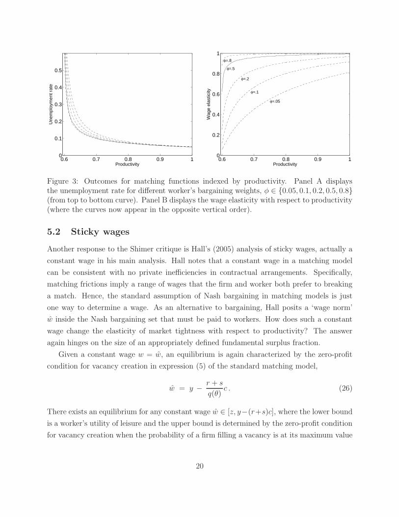
the matching model. We report outcomes from a similar exercise in Figures 3(a) and 3(b)

where we recompute our relationship between unemployment and productivity for different

values of a worker’s bargaining weight φ ∈ {0.05, 0.1, 0.2, 0.5, 0.8}. The solid line in Figure

3(a) with φ = 0.5 depicts the same curve that appeared in Figure 1(a). The corresponding

elasticities of wages with respect to productivity are depicted in Figure 3(b). We conclude

from Figure 3(a) that high responses of unemployment to changes in productivity occur only

at low fundamental surplus fractions. Figure 3(b) confirms that the Shimer critique of com-

mon calibrations does not hinge on a high wage elasticity and that the Hagedorn-Manovskii

result is not predicated on a low wage elasticity. We provide yet another perspective of these

issues in section 6.2.

In conclusion, we do not deny that common calibrations of the matching model and

the specific alternative calibration of Hagedorn and Manovskii (2008) are characterized by

high and low wage elasticities, respectively; but we do assert that the size of the calibrated

fundamental surplus fraction and not these wage elasticities is the important thing.11

11For a further discussion of the determinants of the wage elasticity, see online appendix B. Also, at theend of that appendix, we provide an explanation of why the wage elasticities in Figure 2 are higher thanthose for the solid line (φ = 0.5) in Figure 3(b).

19

0.6 0.7 0.8 0.9 10

0.1

0.2

0.3

0.4

0.5

Une

mpl

oym

ent r

ate

Productivity0.6 0.7 0.8 0.9 1

0

0.2

0.4

0.6

0.8

1

Wag

e el

astic

ity

Productivity

φ=.8

φ=.5

φ=.2

φ=.1

φ=.05

Figure 3: Outcomes for matching functions indexed by productivity. Panel A displaysthe unemployment rate for different worker’s bargaining weights, φ ∈ {0.05, 0.1, 0.2, 0.5, 0.8}(from top to bottom curve). Panel B displays the wage elasticity with respect to productivity(where the curves now appear in the opposite vertical order).

5.2 Sticky wages

Another response to the Shimer critique is Hall’s (2005) analysis of sticky wages, actually a

constant wage in his main analysis. Hall notes that a constant wage in a matching model

can be consistent with no private inefficiencies in contractual arrangements. Specifically,

matching frictions imply a range of wages that the firm and worker both prefer to breaking

a match. Hence, the standard assumption of Nash bargaining in matching models is just

one way to determine a wage. As an alternative to bargaining, Hall posits a ‘wage norm’

w inside the Nash bargaining set that must be paid to workers. How does such a constant

wage change the elasticity of market tightness with respect to productivity? The answer

again hinges on the size of an appropriately defined fundamental surplus fraction.

Given a constant wage w = w, an equilibrium is again characterized by the zero-profit

condition for vacancy creation in expression (5) of the standard matching model,

w = y − r + s

q(θ)c . (26)

There exists an equilibrium for any constant wage w ∈ [z, y−(r+s)c], where the lower bound

is a worker’s utility of leisure and the upper bound is determined by the zero-profit condition

for vacancy creation when the probability of a firm filling a vacancy is at its maximum value

20

of one, q(θ) = 1. After implicitly differentiating (26), we can compute the elasticity of market

tightness as

ηθ,y =1

α

y

y − w≡ Υsticky y

y − w. (27)

This equation for ηθ,y resembles the earlier one in (15). Not surprisingly, if the constant wage

equals the value of leisure, w = z, then the elasticity (27) is equal to that earlier elasticity

of market tightness in the standard matching model with Nash bargaining when the worker

has a zero bargaining weight, φ = 0. With such lopsided bargaining power, the equilibrium

wage would indeed be the constant value z of leisure.

From this similarity, we are reminded that the first factor in expression (15) can play

a limited role in magnifying the elasticity ηθ,y because it is bounded from above by the

inverse of the elasticity of matching with respect to unemployment, α. In (27) the bound is

attained. So again it is the second factor, the inverse of the fundamental surplus fraction,

that tells whether the elasticity of market tightness is high or low. The proper definition

of the fundamental surplus is now the difference between productivity and the stipulated

constant wage.

In Hall’s (2005) model, all of the fundamental surplus goes to vacancy creation (as also

occurs in the standard matching model with Nash bargaining when the worker’s bargaining

weight is zero). A given percentage change in productivity is multiplied by a factor y/(y − w)

to become a larger percentage change in the fundamental surplus. Because all of the funda-

mental surplus now goes to vacancy creation, there is a correspondingly magnified impact on

unemployment. Our interpretation is born out in numerical simulations of economies with

aggregate productivity shocks in section 7.1.

5.3 Alternating-offer wage bargaining

Hall and Milgrom (2008) proposed another response to the Shimer critique. They replaced

standard Nash bargaining with alternating-offer bargaining. A firm and a worker take turns

making wage offers. The threat is not to break up and receive outside values, but instead

to continue to bargain because that choice has a strictly higher payoff than accepting the

outside option. After each unsuccessful bargaining round, the firm incurs a cost of delay

γ > 0 while the worker enjoys the value of leisure z. There is a probability δ that the job

opportunity is exogenously destroyed between bargaining rounds, sending the worker to the

unemployment pool.

It is optimal for both bargaining parties to make barely acceptable offers. The firm

21

always offers wf and the worker always offers ww. Consequently, in an equilibrium, the first

wage offer is accepted. Hall and Milgrom assume that firms make the first wage offer.

In their concluding remarks, Hall and Milgrom (2008, p. 1673) choose to emphasize that

“the limited influence of unemployment [the outside value of workers] on the wage results

in large fluctuations in unemployment under plausible movements in [productivity].” But

it is more enlightening to emphasize that once again the key force is that an appropriately

defined fundamental surplus fraction is calibrated to be small. Without a small fundamental

surplus fraction, it matters little that the outside value has been prevented from influencing

bargaining. We illustrate this idea by computing the elasticity of market tightness with

respect to productivity.

After a wage agreement, a firm’s value of a filled job, J , and the value of an employed

worker, E, remain given by expressions (2) and (6) in the standard matching model. These

can be rearranged to become

E =w + β sU

1− β(1− s), (28)

J =y − w

1− β(1− s), (29)

where we have imposed a zero-profit condition on vacancy creation, V = 0, in the second

expression. Thus, using expression (28), the indifference condition for a worker who has just

received a wage offer wf from the firm and is choosing whether to decline the offer and wait

until the next period to make a counteroffer ww is

wf + β sU

1− β(1− s)= z + β

[(1− δ)

ww + β sU

1− β(1− s)+ δ U

]. (30)

Using expression (29), the analogous condition for a firm contemplating a counteroffer from

the worker isy − ww

1− β(1− s)= −γ + β(1− δ)

y − wf

1− β(1− s). (31)

After collecting and simplifying the terms that involve the worker’s outside value U ,

expression (30) becomes

wf

1− β(1− s)= z + β(1− δ)

ww

1− β(1− s)+ β

1− β

1− β(1− s)(δ − s)U. (32)

22

As emphasized by Hall and Milgrom, the worker’s outside value U has a small influence on

bargaining; when δ = s, the outside value disappears from expression (32). That is, under

continuing bargaining that ends only either with an agreement or with destruction of the

job, the outside value will matter only if the job destruction probability differs before and

after reaching an agreement. To strengthen Hall and Milgrom’s (2008) observation that

the outside value has at most a small influence under their bargaining protocol, we proceed

under the assumption that δ = s, so the two indifference conditions (32) and (31) become

wf = (1− β) z + β ww, (33)

y − ww = −(1− β) γ + β (y − wf) , (34)

where β ≡ β(1− s). Solve for ww from (34) and substitute into (33) to get

wf =(1− β)

[z + β(y + γ)

]1− β2

=z + β(y + γ)

1 + β. (35)

This is the wage that a firm would immediately offer a worker when first matched; the offer

would be accepted.12 In an equilibrium, this wage must also be consistent with the no-profit

condition in vacancy creation. Substitution of w = wf from expression (35) into the no-

profit condition (5) of the standard matching model results in the following expression for

equilibrium market tightness:

z + β(y + γ)

1 + β= y − r + s

q(θ)c. (36)

After implicit differentiation, we can compute the elasticity of market tightness as

ηθ,y =1

α

y

y − z − β γ, (37)

where the fundamental surplus is the productivity that remains after making deductions for

the value of leisure z and a firm’s discounted cost of delay βγ. The latter item captures the

worker’s prospective gains from his ability to exploit the cost that delay imposes on the firm.

What remains of productivity is the fundamental surplus that could potentially be extracted

12When firms make the first wage offer, a necessary condition for an equilibrium is that wf in expression(35) is less than productivity y, i.e., the parameters must satisfy z + βγ < y.

23

by the ‘invisible hand’ and devoted to sustaining vacancy creation in an equilibrium.

While Hall and Milgrom (2008, p. 1670) notice that their “sum of z and γ is . . . not

very different from the value of z by itself in . . . Hagedorn and Manovskii’s calibration” (as

studied in our section 5.1), they downplay this similarity and choose to emphasize differences

in mechanisms across Hagedorn and Manovskii’s model and theirs. But properly focusing

on the fundamental surplus tells us that it is their similarity that should be stressed – the

two models are united in requiring a small fundamental surplus fraction to generate high

unemployment volatility over the business cycle.

To summarize, we do not doubt that the alternative bargaining protocol of Hall and

Milgrom (2008) suppresses the influence of the worker’s outside value during bargaining. But

this outcome would be irrelevant had Hall and Milgrom not calibrated a small fundamental

surplus fraction.

5.4 A financial accelerator

Wasmer and Weil (2004) explore how a financial accelerator affects the elasticity of labor

market tightness with respect to productivity. They assume that matching in a credit market

precedes matching in the labor market. Credit matching determines equilibrium measures e

and f of entrepreneurs and financiers, respectively, the two inputs into a matching function

for the credit market. Matched entrepreneur-financier pairs then post vacancies in a matching

function for labor. As before, the labor market matching function matches vacancies with

workers. Filled jobs and the entrepreneur-financier matches that helped to create them are

exogenously destroyed with per-period probability s.

The credit market matching function has constant returns to scale. Credit market tight-

ness σ ≡ e/f determines the probability p(σ) (σp(σ)) that an entrepreneur (a financier) finds

a counterparty. Per-period credit market search costs of an entrepreneur and a financier

are denoted ε > 0 and κ > 0, respectively. A successfully matched entrepreneur-financier

pair immediately posts one vacancy in the matching function for the labor market. An

entrepreneur-financier pair shares the value of a vacancy according to Nash bargaining, ξ

and 1− ξ being the bargaining power of the entrepreneur and the financier, respectively. In

their main setup, Wasmer and Weil (2004) assume a sticky wage w in the labor market. The

key question ultimately to be studied is how the elasticity of labor market tightness differs

from that of Hall’s (2005) sticky wage model described above in section 5.2.

In an equilibrium, costly search in the credit market assumes a strictly positive value

24

of a vacancy in the labor market, V > 0. Nash bargaining awards the entrepreneur and

the financier ξV and (1 − ξ)V , respectively. Free entry on both sides of the credit market

ensures that the two parties expect to break even, so that the per-period search costs of an

entrepreneur and a financier equal their respective expected payoffs:

ε = p(σ)ξV and κ = σp(σ)(1− ξ)V. (38)

The zero expected profits conditions (38) imply that the equilibrium value of a vacancy

in the labor market equals total search costs in the credit market divided by the number

of entrepreneur-financier pairs formed, which is the average search cost incurred for the

formation of an entrepreneur-financier pair in the credit market:

V =ε

p(σ)+

κ

σp(σ)≡ K(σ). (39)

The zero expected profits conditions (38) also imply that equilibrium credit market tightness

σ is a function solely of relative bargaining powers and relative per-period search costs,

σ =1− ξ

ξ

κ

ε≡ σ�. (40)

The value of a vacancy continues to be given by equation (3), which can be solved for

the value of a filled job

J =1

βq(θ)

[c +

(1− β[1− q(θ)]

)K(σ�)

], (41)

where we have invoked equilibrium outcomes (39) and (40), i.e., V = K(σ�). Another

expression for the value J of a filled job is obtained by solving a pertinent version of Bellman

equation (2), namely,13

J = y − w + β(1− s)J ,

“forward” to obtain

J =y − w

β(r + s). (42)

The equilibrium value of labor market tightness θ adjusts to equate expressions (41) and

13Note that upon the destruction of a job in the Wasmer and Weil setup, the entrepreneur-financier pairalso breaks up so that the value of a vacancy V vanishes in the Bellman equation (2).

25

(42) for the value J of a filled job

q(θ)[y − w − (r + s)βK(σ�)

]= (r + s)

[c + (1− β)K(σ�)

]. (43)

After implicit differentiation, we can compute the elasticity of market tightness as

ηθ,y =1

α

y

y − w − k. (44)

where k ≡ (r + s)βK(σ�). Comparing (44) to the elasticity (27) that emerges from Hall’s

(2005) sticky wage model, we observe that (44) deducts another term k from the funda-

mental surplus, namely, the annuitized value of the average search costs incurred to form

an entrepreneur-financier pair.14 In the Wasmer and Weil setup, the invisible hand cannot

use these resources to pay for vacancy costs in the labor market, since they are required to

assure that entrepreneur-financier pairs on average earn zero expected profits from investing

in credit market search costs.15 16

14To have the same expected present value as the average search costs in the credit market, K(σ�), wecompute an annuity k with a stream that starts when an entrepreneur-financier pair matches with a worker,and ends at the job’s stochastic destruction:

∞∑t=0

βt(1− s)tk = K(σ�) =⇒ k = (r + s)βK(σ�) .

15Petrosky-Nadeau and Wasmer (2013, first equation on page 201) construe a multiplicative role of thefinancial accelerator in Wasmer andWeil’s model, as said to be represented by the second factor J/(J−K(σ�))in the following steady-state version of their expression for the elasticity of market tightness,

ηθ,y =1

α

J

J −K(σ�)

y

y − w.

Though, after invoking equilibrium expression (42) for the value J of a filled job, our expression (44) forthe elasticity reemerges. Hence, we conclude that there is no multiplicative role of the financial acceleratorbut rather, the annuitized value of the average search costs in the credit market simply diminishes thefundamental surplus.

16For the elasticity of market tightness under Nash-bargained wages in the Wasmer and Weil setup, seeonline appendix A.6 where we adopt the block-bargaining assumption of Petrosky-Nadeau and Wasmer’s(2013) extension, i.e., the entrepreneur and the financier form a block when bargaining with the worker.The resulting decomposition of the elasticity of market tightness for this setting resembles the case of a fixedmatching cost incurred by the firm before bargaining with the worker. (See footnote 10.)

26

6 Fundamental surpluses and profits

To shed further light on why a small fundamental surplus fraction is necessary for small

changes in productivity to have large effects on unemployment, we examine the chain of

causality that operates through the relative impact of productivity on firms’ profits. We

use the fact that, in an equilibrium, free entry into job creation implies that the expected

present value of a firm’s profits is related to the average vacancy expenditures for filling a

job. Except for models of layoff taxes, fixed matching costs, and a financial accelerator, all

our preceding derivations of analytical expressions for the elasticity of market tightness with

respect to productivity involve the equilibrium condition:17

c = β q(θ)y − w(y, θ)

1− β(1− s), (45)

where we have substituted expression (29), the value of a job expressed as the expected

present value of its profits, into break-even condition (4) for vacancy creation. For each

particular model, the equilibrium wage w(y, θ) is a nondecreasing function in productivity y

and market tightness θ.

Differentiating expression (45) with respect to y and θ yields

ηθ,y =1

α

[1− wy(y, θ)− wθ(y, θ)

d θ

d y

]y

y − w(y, θ), (46)

which is an alternative to our earlier formulas (15), (27) and (37) for the elasticity of matching

with respect to productivity. It is a decomposition into three multiplicative components. As

discussed above, the magnitude of the first component 1/α is restricted by a consensus about

what are reasonable estimates of the elasticity α. Delineated by square brackets, the second

component involves nonnegative derivatives of the wage and the positive derivative of market

tightness with respect to productivity. An upper bound of unity for the second component

would be attained if wy = wθ = 0. Thus, we conclude that a necessary condition for

expression (46) to be really large is that its third component is large, i.e., for any possibility

of market tightness to respond sensitively to small changes in productivity, a firm’s profit

relative to productivity, (y − w)/y, must be small.

Interpretations of the three multiplicative components in expression (46) are straight-

17The argument below can easily be modified so that the conclusions extend to the models of layoff taxes,fixed matching costs, and a financial accelerator.

27

forward. The second component is the fraction of an increment in productivity that is not

siphoned off to the wage but passed on to a firm’s profit. In relative terms, any change in

productivity that is passed on to profits translates into a greater percentage change in profits

by a factor of y/(y−w), i.e., the third component. The first component 1/α determines then

how these dynamics map into an elasticity of market tightness with respect to productivity,

where the free-entry condition in vacancy creation ensures that the relative change in a firm’s

profit is also the relative change in average vacancy expenditures for filling a job. The larger

such a relative change in vacancy expenditures caused by a change in productivity, the larger

is the elasticity of market tightness with respect to productivity.

To understand how these observations square with the all-important concept of the fun-

damental surplus fraction, we start by considering instances when the wage is invariant to

market tightness, and then proceed to studying outcomes under Nash bargaining.

6.1 Wage invariant to market tightness

If the wage w(y) is a function solely of productivity, expression (46) simplifies to become

ηθ,y =1

α[1− w′(y)]

y

y − w(y). (47)

In the case of a constant wage in section 5.2, w(y) = w and w′(y) = 0, this is immediately

seen to be our earlier expression (27). As already discussed, the firm’s profit then coincides

with the fundamental surplus.

Another example of a wage invariant to market tightness is the outcome under alternating-

offer bargaining in section 5.3 when the parameterization is such that outside values have no

influence on bargaining (δ = s). Under the assumption that firms formulate the first wage

offer, we can use equilibrium wage expression (35) to compute

w′(y) =β

1 + βand y − w(y) =

y − z − βγ

1 + β. (48)

Given the constancy of derivative w′(y) in (48), the second component of expression (47) is

also a constant (less than one). Hence, attaining a high elasticity of market tightness can

focus on making the third component large, i.e., making profit small. As compared to the

fundamental surplus identified in expression (37), we see that a firm’s profit y−w(y) in (47)

constitutes a constant fraction (1 + β)−1 of the fundamental surplus.

28

Thus, two common calibration targets are well aligned in these frameworks: (1) a high

elasticity of market tightness with respect to productivity chosen to generate business cy-

cle fluctuations, and (2) small profits chosen to be consistent with data on small vacancy

expenditures relative to output. Hitting both targets is helped by setting a sufficiently

high constant wage in the sticky-wage model, or a sufficiently high firm’s cost of delay in

bargaining in the alternating-offer bargaining model (for a given value of leisure).

Things get more complicated under Nash bargaining, to which we turn next. While a

small fundamental surplus fraction trivially implies small profits (because the former is an

upper bound on what the ‘invisible hand’ could ever allocate to vacancy creation and the

latter reflects what is actually allocated in an equilibrium), small profits are no longer a sure

indication of the size of the fundamental surplus fraction.

6.2 Wage under Nash bargaining

As discussed and refuted in section 5.1, a prominent explanation for the low elasticity of mar-

ket tightness with respect to productivity in common calibrations of the standard matching

model is that the elasticity of wages with respect to productivity is too high. Rogerson and

Shimer (2011) misattribute the success of Hagedorn and Manovskii (2008) in raising the

elasticity of market tightness to their calibration of a rigid wage. To supplement our earlier

numerical counterexamples and discussion of the steady-state comparative-statics expression

(15) for the elasticity of market tightness (as well as for the wage elasticity in online ap-

pendix B), our expression (46) for the elasticity of market tightness can be used to provide

yet another perspective on these issues.

For a given value of leisure z, recall that we generated different wage elasticities by varying

a worker’s bargaining weight φ. The striking finding is that the elasticity of market tightness

is almost invariant to such perturbations. In terms of expression (46), the explanation is

that varying a worker’s bargaining weight φ has countervailing effects on the second and

third components. Hagedorn and Manovskii (2008, p. 1696) summarize their explorations:

“What matters for the incentives to post vacancies is the size of the percentage changes of

profits in response to changes in productivity. These percentage changes are large if the

size of profits is small and the increase in productivity is not fully absorbed by an increase

in wages. In the standard [matching] model, conditional on the choice of z, the bargaining

parameter [φ] determines both the level and the volatility of wages. Thus, if we fix z and

raise [φ], wages rise and become more cyclical, meaning that profits become smaller but

29

less cyclical. These two opposing effects almost exactly cancel each other out. Thus, the

volatility of labor market tightness is almost independent of [φ] and is determined only by

the level of z.”

While our formula (46) cast in terms of endogenous quantities symptomizes these coun-

tervailing forces, it cannot tell us whether that invariant elasticity of market tightness is

low or high. But after evaluating formula (46), by invoking wage expression (11) and using

equilibrium condition (12) to eliminate intermediate variables, our earlier expression (15)

reemerges. Once again, it is abundantly clear that the elasticity of market tightness “is

determined only by the level of z,” or more properly, by the fundamental surplus fraction

(y − z)/y.

6.3 Profits under Nash bargaining

It is useful to compute the relationship of the fundamental surplus to a firm’s portion of the

match surplus, namely, a firm’s profits. After substituting Nash bargaining outcome (8) into

break-even condition (4) for vacancy creation, the equilibrium condition c = βq(θ)(1− φ)S

emerges, which when substituted into equilibrium condition (12) yields

S =1 + r

r + s+ φ θ q(θ)(y − z). (49)

In section 7, to study effects of alternative parameter values, we will draw isoquants for the

match surplus. So suppose that a parameterization in expression (49) has the same match

surplus as an alternative parameterization indexed by the superscript star, i.e., S = S�, so

that1 + r

r + s+ φ θ q(θ)(y − z) =

1 + r�

r� + s� + φ� θ� q�(θ�)(y − z�). (50)

Further, let the two parameterizations share the same interest rate, r = r�, and separation

rate, s = s�, and also let each matching function be calibrated to target the same unemploy-

ment rate, i.e., by expression (13), the job finding rates will be the same, θq(θ) = θ�q�(θ�),

so that expression (50) can be rearranged to read,

y − z

y − z�=

r + s+ φ θ q(θ)

r + s + φ� θ q(θ). (51)

To arrive at an analogous expression for isoprofit curves, we simply multiply the left and

right sides of expression (49) by (1− φ). Then, we follow the same steps as above, but now

30

for two parameterizations with the same value for a firm’s profits, (1 − φ)S = (1 − φ�)S�,

which yieldsy − z

y − z�=

1− φ�

1− φ

r + s+ φ θ q(θ)

r + s+ φ� θ q(θ). (52)

According to expressions (51) and (52), along an isoquant for the match surplus or for a

firm’s profits, a smaller fundamental surplus is associated with a lower worker’s bargaining

power. Could this be the reasoning underlying the common attributions of high elasticities

of market tightness to low elasticities of the wage with respect to productivity? (See section

5.1.) Although we are unaware of earlier such rationalizations, it is evidently true that hold-

ing the match surplus or a firm’s profits constant, the fundamental surplus (fraction) and

a worker’s bargaining power move in opposite directions. Hence, a higher fundamental sur-

plus fraction increases the elasticity of market tightness and the associated lower bargaining

power of a worker decreases the elasticity of the wage with respect to productivity.

But as the numerical analysis of the next section will illustrate, when we allow for the

match surplus to change across parameterizations, relationships between the elasticities of

market tightness and the wage vanish. Instead, expression (15) is back in full force, making

the fundamental surplus fraction the sole determinant of the elasticity of market tightness.

The quantitative analysis in section 7.2 demonstrates how small match surpluses or small

firms’ profits are unreliable indicators of the elasticity of market tightness in Nash bargaining

models.

7 Business cycles

To illustrate how a small fundamental surplus fraction is essential for generating ample unem-

ployment volatility over the business cycle in matching models, we turn to Hall’s (2005) spec-

ification with discrete time and a random productivity process. The monthly discount factor

β corresponds to a 5-percent annual rate and the value of leisure is z = 0.40. The elasticity of

matching with respect to unemployment is α = 0.235, and the exogenous monthly separation

rate is s = 0.034. Aggregate productivity takes on five values ys uniformly spaced around a

mean of one on the interval [0.9935, 1.00565], and is governed by a monthly transition prob-

ability matrix Π with probabilities that are zero except as follows: π1,2 = π4,5 = 2(1 − ρ),

π2,3 = π3,4 = 3(1 − ρ), with the upper triangle of the transition matrix symmetrical to the

lower triangle and the diagonal elements equal to one minus the sums of the nondiagonal

elements. The resulting serial correlation of y is ρ, which is parameterized to be ρ = 0.9899.

31

However, to facilitate our sensitivity analysis, we alter Hall’s model period from one month

to one day. (See online appendix C.) As mentioned in footnote 6, a shorter model period

fosters the existence of equilibria with vacancy creation.

7.1 Hall’s (2005) sticky wage model

As in Hall’s (2005) analysis of a constant wage, we postulate a fixed wage w = 0.9657,

which equals the flexible wage that would prevail at the median productivity level under

standard Nash bargaining (with equal bargaining weights, φ = 0.5). Figure 4(a) reproduces

Hall’s figures 2 and 4 for those two models. The solid line and the upper dotted line depict

unemployment rates at different productivities for the sticky-wage model and the standard

Nash-bargaining model, respectively.18 Unemployment is almost invariant to productivity

under Nash bargaining but responds sensitively under the sticky wage. The outcomes are

explained by differences in job-finding rates as shown by the dashed line and the lower

dotted line for the sticky-wage model and the standard Nash-bargaining model, respectively,

expressed at our daily frequency.19 Under the sticky wage, high productivity causes firms to

post many vacancies, making it easy for unemployed workers to find jobs, while the opposite

is true when productivity is low.

Starting from this verification of our conversion of Hall’s (2005) model into a daily fre-

quency, we conduct a sensitivity analysis of the choice of the fixed wage. The solid line in

Figure 4(b) shows how the average unemployment rate varies with the fixed wage w. Note

how a small range of wages spans outcomes from a very low to a very high average unem-

ployment rate. Small variations in a fixed wage close to productivity generate large changes

in the fundamental surplus fraction, (y − w)/y, which by free entry of firms map directly

into the amount of resources devoted to vacancy creation. The dashed line in Figure 4(b)

traces out the implications for the volatility of unemployment. The standard deviation of

unemployment is nearly zero at the left end of the graph when the job-finding probability

is almost one for all productivity levels. Unemployment volatility then increases for higher

constant wages until, outside of the graph at the right end, vacancy creation becomes so

18Unemployment is a state variable that is not just a function of the current productivity, as are all ofthe other variables, but depends on the history of the economy. But high persistence of productivity andthe high job-finding rates make the unemployment rate that is observed at a given productivity level be wellapproximated by expression (13) evaluated at the market tightness θ prevailing at that productivity (seeHall (2005, p. 59)).

19Our daily job-finding rates are roughly 1/30 of the monthly rates in Hall (2005, figures 2 and 4),confirming our conversion from a monthly to a daily frequency.

32

0.994 0.996 0.998 1 1.002 1.004 1.0061

2

3

4

5

6

7

8

9

Productivity

%

Unemployment rateJob finding rate

0.95 0.955 0.96 0.965 0.97 0.975 0.980

2

4

6

8

10

Fixed wage

%

mean(u)std(u)

Hall’s Fixed Wage

Figure 4: Outcomes in the sticky-wage model. Panel A displays unemployment rates anddaily job-finding rates at different productivities (given a fixed wage w = 0.9657), wherethe dotted lines with almost no slopes are counterparts from a standard Nash-bargainingmodel. Panel B displays the average unemployment rate and the standard deviation ofunemployment for different postulated values of the fixed wage.

unprofitable that average unemployment converges to its maximum of 100 percent and there

are no more fluctuations.

At Hall’s fixed wage w = 0.9657, Figure 4(b) shows a standard deviation of unemployment

equal to 1.80 percentage points, which is close to the target of 1.54 to which Hall (2005)

calibrated his model. Next, we will see how the standard Nash-bargaining model can attain

the same volatility of unemployment by elevating the value of leisure.

7.2 Hagedorn and Manovskii’s (2008) high value of leisure

Using Hall’s (2005) parameters but assuming standard Nash wage bargaining, we revisit the

analysis of Hagedorn and Manovskii (2008) by postulating a high value of leisure, z = 0.960,

and a low bargaining power of workers, φ = 0.0135. For those parameter values, we do indeed

obtain a high standard deviation of 1.4 percentage points for unemployment. To shed light

on the sensitivity of outcomes to the choice of parameters, Figure 5(a) depicts outcomes for

different constellations of z ∈ [0.4, .99] and φ ∈ [0.001, 0.5]. For each pair (z, φ), we adjust

the efficiency parameter A of the matching function to make the average unemployment rate

be 5.5 percent. As we would expect, a high value of leisure, i.e., a small fundamental surplus

fraction, is essential for obtaining large variations in market tightness and a high volatility

of unemployment.

33

As detailed in section 5.1 (and elaborated upon in online appendix B), Hagedorn and

Manovskii (2008) require a low bargaining power of workers to match the elasticity of

wages with respect to productivity. When we revisit their argument based on (z, φ) =

(0.960, 0.0135) in the otherwise same parametrized environment of Hall (2005), the resulting

wage elasticity of 0.44 is approximately the value to which Hagedorn and Manovskii cali-

brated their original analysis. Following the computational approach in Figure 5(a), Figure

5(b) provides a sensitivity analysis for the choice of parameter values (z, φ). The figure

verifies the necessity for a low φ to obtain a low wage elasticity.

Taken together, Figures 5(a) and 5(b) show how the low wage elasticity of Hagedorn

and Manovskii (2008) is incidental to and neither necessary nor sufficient to obtain a high

volatility of unemployment. Hence, earlier misinterpretations stressing the importance of

a rigid wage (Rogerson and Shimer 2011) should be set aside and replaced by the correct

statement that the fundamental surplus fraction must be small.

A deceptive first impression of Figure 5(c) is that the match surplus might also be closely

related to the elasticity of market tightness, because small match surpluses at values of

leisure close to one coincide with high standard deviations of unemployment in Figure 5(a).

But this outcome follows merely from the fact that the fundamental surplus is an upper

bound on resources that the invisible hand can allocate to vacancy creation and hence, when

the fundamental surplus becomes tiny at values of leisure close to one, the match surplus

must also become small. To appreciate the forces actually driving outcomes, we should

check if isoquants for the match surplus line up with isoquants for the standard deviation of

unemployment, as they clearly do for the fundamental surplus. The diagonal dashed line in

Figure 5(d) is the isoquant for the match surplus of Hall’s (2005) version of a Nash bargaining

model with parameter values z = 0.4 and φ = 0.5. Since Hall’s parameterization exemplifies

a common calibration of the standard matching model, it follows that the elasticity of market

tightness and the standard deviation of unemployment are small. However, to the northwest

along that same isoquant in Figure 5(d), there are other Hagedorn-Manovskii (2008) like

calibrations with the exactly same match surplus but with much higher standard deviations

of unemployment. This reasoning leads us to conclude that the size of the match surplus is

not a good indicator of the elasticity of market tightness.

A similar message is conveyed by the isoprofit curves in Figure 5(d): the three solid curves

with the middle one representing a firm’s profits in Hall’s (2005) Nash bargaining model.

Recall our discussion in the introduction of Hagedorn and Manovskii’s (2008) discerning

observation that profits need to be small and elastic for unemployment to respond sensitively

34

0

0.2

0.40.4

0.6

0.8

10

0.5

1

1.5

2

2.5

Flow value of leisureBargaining power

std(

u) in

%

Hagedorn − Manovskii

(a) Std of unemployment

0

0.2

0.40.4

0.60.8

1

0

0.2

0.4

0.6

0.8

1

Flow value of leisureBargaining power

Ela

stic

ity

Hagedorn − Manovskii

(b) Wage elasticity

00.1

0.20.3

0.40.4

0.6

0.8

10

100

200

300

400

Flow value of leisureBargaining power

Ave

rage

mat

ch s

urpl

us

(c) Match surplus

Bargaining power

Flo

w v

alue

of l

eisu

re

0 0.1 0.2 0.3 0.4 0.50.4

0.5

0.6

0.7

0.8

0.9

1

(d) Isoprofit curves (solid)

Figure 5: Outcomes in the Nash-bargaining model for different constellations of the value ofleisure z, and the bargaining power of workers φ. Panel (a) displays the standard deviationof unemployment in percentage points. Panel (b) shows the wage elasticity with respectto productivity. Panel (c) depicts the match surplus. In panel (d), the diagonal dashedline is an isoquant for the match surplus distilled from panel (c), the three solid lines areisoprofit curves, and the three dotted curves are isoquants for the standard deviation ofunemployment in panel (a).

35

to movements in productivity. Along the top two isoprofit curves or any higher ones not

shown in Figure 5(d), profits are held constant at relatively low levels. But for any such small

profits to be elastic also with respect to changes in productivity, i.e., for small profits to be

associated with high standard deviations of unemployment, the fundamental surplus fraction

must be small in Figure 5(d). We are again reminded that the fundamental surplus fraction

is the determinant of the elasticity of market tightness, and that small match surpluses or

small firms’ profits are unreliable indicators thereof.20

7.3 Hall and Milgrom’s (2008) alternating-offer bargaining

Finally, we turn to Hall and Milgrom’s (2008) model of alternating-offer wage bargaining as

another way to increase unemployment volatility in a matching framework. Except for the

wage formation process, their environment is the same as that of Hall (2005) but parame-

terized quite differently. It is important to stress one difference between Hall and Milgrom’s

parameterization and that of Hall (2005) because it plays an important role in setting the

fundamental surplus: they raised the value of leisure to z = 0.71 from Hall’s value of z = 0.40.

Section 5.3 taught us that the value of leisure and the firm’s cost of delay in bargaining (γ)

are likely to be critical determinants of the elasticity of market tightness with respect to

productivity and hence of the volatility of unemployment.

Hall and Milgrom (2008) choose instead to emphasize how much the outside value of un-

employment is suppressed in alternating-offer wage bargaining since disagreement no longer

leads to unemployment but instead to another round of bargaining. Hence, a key parame-

ter from Hall and Milgrom’s perspective is the exogenous rate δ at which parties break up

between bargaining rounds. Figure 6 shows how different constellations of (γ, δ) affect the

standard deviation of unemployment. For each pair (γ, δ), we adjust the efficiency parame-

ter A of the matching function to make the average unemployment rate be 5.5 percent. For

the record, Hall and Milgrom (2008) argue that productivity shocks are not the sole source

of unemployment fluctuations and consequently they lower their target standard deviation

of unemployment to 0.68 percentage points – a target attained with their parameterization

(γ, δ) = (0.27, 0.0055) and reproduced in Figure 6.

Figure 6 supports our earlier finding that the cost of delay γ together with the value of

leisure z are paramount for generating higher volatility of unemployment. Without a cost of

20The isoquant for the match surplus and the isoprofit curves in Figure 5(d) depict averages in ourstochastic specification of the Nash bargaining model. The steady-state expressions (51) and (52) providealmost perfect approximations to those outcomes.

36

0.240.260.280.30.322345 x 10

−3

0.5

1

1.5

2

2.5

Sep. while bargainingCost of delay

std(

u) in

%

Hall and Milgrom

Figure 6: The standard deviation of unemployment in percentage points for different con-stellations of firms’ cost of delay in bargaining (γ) and the exogenous separation rate whilebargaining (δ) in the alternating-offer bargaining model.

delay sufficiently high to reduce the fundamental surplus fraction, the exogenous separation

rate between bargaining rounds matters little.21

8 More complicated environments

To watch the fundamental surplus working its will in more complicated environments, we

investigate the roles of matching models in Hornstein et al. (2007) and Christiano et al.

(2015). For further details on our two explorations, see online appendix D.

8.1 A suite of welfare state policies

Hornstein et al. (2007) (henceforth HKV) put a matching function into a model with vintage

capital and use it to argue a substantial increase in European unemployment to an acceler-

ation in the rate of capital-embodied technological change �. HKV suggest that pre-1970

and post-1990 periods are characterized by � = 0.04 and � = 0.077, respectively, which

together with HKV’s assumptions about government policies for them explains why the un-

employment rate increased in post-1990 by over four percentage points in Europe but by

21To be specific, our formula (37) for the steady-state comparative statics is an approximation of theelasticity of market tightness at the rear end of Figure 6 where the exogenous rate δ at which parties breakup between bargaining rounds is equal to Hall and Milgrom’s (2008) assumed job destruction rate of 0.0014per day.

37

just one percentage point in the U.S.

In HKV’s framework, the formation of a job coincides with investing in a one-worker

machine with capital-embodied productivity at the frontier of an exogenously moving tech-

nology frontier at the time of investment. The two inputs into their single matching function

are homogeneous unemployed workers and vacant machines of different vintages. Matched

worker-machine pairs engage in Nash bargaining to set vintage-specific wage rates. All

worker-machine pairs are subject to exogenous separation shocks that return separated work-

ers and machines to the matching function. When the capital-embodied productivity of a

vintage falls too far behind the current technology frontier, the match surplus evaporates

and machines are scrapped.

HKV calibrate government policies to be more active in Europe than in the U.S.: un-

employment benefits bEU = 0.33 versus bUS = 0.05, which correspond to replacement rates

of 75% and 10% of average wages in pre-1970 (when � = 0.04) in Europe and the U.S.,

respectively; a layoff tax τEU = 0.45 in Europe, which is equivalent to one year of average

wages in pre-1970 (when � = 0.04) versus no layoff tax in the U.S.; and a pair of European

income and payroll taxes {24%, 21%} versus a U.S. pair {17%, 8%}. To generate balanced

growth paths, HKV assume that unemployment benefits b, layoff taxes τ , and the investment

cost for machines change at the economy’s growth rate.22

To understand how � affects unemployment outcomes, we compare with the forces at

work earlier in Figure 1(a). A higher � acts as an obsolescence shock because it shortens

the equilibrium lifespan of machines, leaving less time to recover the machine cost. Holding

other things the same, a shorter machine life also implies that the annuity value of the layoff

tax increases and that the fundamental surplus falls (in line with our discussion of expression

(23)). But other things are not the same – the fundamental surplus now shrinks faster with

the age of a machine since both the unemployment benefit and the layoff tax grow at the

economy’s growth rate, which has risen as a consequence of a higher � (while the vintage-

dependent output evolves over a machine’s lifespan in the same way as before). The implied

reduction in the fundamental surplus fraction can be thought of as a leftward movement along

the curve in a graph like Figure 1(a). Thus, HKV’s finding of a larger increase in European

unemployment is a manifestation of how welfare state policies had already diminished an

initial fundamental surplus fraction. Consequently, Europe was positioned farther to the

left along the curve in a graph like Figure 1(a) before the onset of higher capital-embodied

22To attain the same unemployment rate of 4% in both Europe and the U.S. in pre-1970, HKV assume asignificantly lower exogenous separation rate in Europe than in the U.S. which remain fixed over time.

38

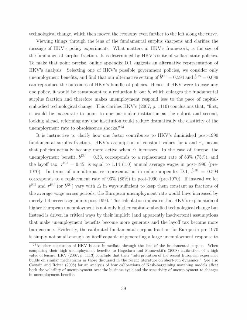
technological change, which then moved the economy even further to the left along the curve.

Viewing things through the lens of the fundamental surplus sharpens and clarifies the

message of HKV’s policy experiments. What matters in HKV’s framework, is the size of

the fundamental surplus fraction. It is determined by HKV’s suite of welfare state policies.

To make that point precise, online appendix D.1 suggests an alternative representation of

HKV’s analysis. Selecting one of HKV’s possible government policies, we consider only

unemployment benefits, and find that our alternative setting of bEU = 0.594 and bUS = 0.089

can reproduce the outcomes of HKV’s bundle of policies. Hence, if HKV were to ease any

one policy, it would be tantamount to a reduction in our b, which enlarges the fundamental

surplus fraction and therefore makes unemployment respond less to the pace of capital-

embodied technological change. This clarifies HKV’s (2007, p. 1110) conclusions that, “first,

it would be inaccurate to point to one particular institution as the culprit and second,

looking ahead, reforming any one institution could reduce dramatically the elasticity of the

unemployment rate to obsolescence shocks.”23

It is instructive to clarify how one factor contributes to HKV’s diminished post-1990

fundamental surplus fraction. HKV’s assumption of constant values for b and τ , means

that policies actually become more active when � increases. In the case of Europe, the

unemployment benefit, bEU = 0.33, corresponds to a replacement rate of 83% (75%), and

the layoff tax, τEU = 0.45, is equal to 1.14 (1.0) annual average wages in post-1990 (pre-

1970). In terms of our alternative representation in online appendix D.1, bEU = 0.594

corresponds to a replacement rate of 93% (85%) in post-1990 (pre-1970). If instead we let

bEU and τEU (or bEU) vary with � in ways sufficient to keep them constant as fractions of

the average wage across periods, the European unemployment rate would have increased by

merely 1.4 percentage points post-1990. This calculation indicates that HKV’s explanation of

higher European unemployment is not only higher capital-embodied technological change but

instead is driven in critical ways by their implicit (and apparently inadvertent) assumptions

that make unemployment benefits become more generous and the layoff tax become more

burdensome. Evidently, the calibrated fundamental surplus fraction for Europe in pre-1970

is simply not small enough by itself capable of generating a large unemployment response to

23Another conclusion of HKV is also immediate through the lens of the fundamental surplus. Whencomparing their high unemployment benefits to Hagedorn and Manovskii’s (2008) calibration of a highvalue of leisure, HKV (2007, p. 1113) conclude that their “interpretation of the recent European experiencebuilds on similar mechanisms as those discussed in the recent literature on short-run dynamics.” See alsoCostain and Reiter (2008) for an analysis of how calibrations of Nash-bargaining matching models affectboth the volatility of unemployment over the business cycle and the sensitivity of unemployment to changesin unemployment benefits.

39

the postulated increase in technological change.

8.2 Nash versus alternating-offer bargaining

Within a DSGE model with habit formation in preferences, adjustment costs in capital for-

mation, capacity utilization costs, Calvo sticky price frictions, and a Taylor rule for monetary

policy, Christiano et al. (2015) (henceforth CET) incorporate a matching model, either with

Nash bargaining or with Hall and Milgrom’s (2008) alternating-offer bargaining (AOB), to

study how labor markets respond to neutral and investment-specific technology shocks and

monetary policy shocks. CET show that their estimated Nash and AOB models equally

well account for patterns in the data and they “generate impulse response functions that are

virtually identical to each other.”

The principle difference in parameter estimates is the replacement rate from unemploy-

ment insurance: 0.88 in the Nash model versus 0.37 in the AOB model. CET find that

restricting the replacement rate in the Nash model to be the same as that of the AOB model

and then recalculating the impulse response functions “leads to a dramatic deterioration in

the performance of the Nash model. All of the quantity variables like hours worked, real

GDP as well as unemployment are now much less responsive to a monetary policy shock

. . . [there is] a similar pattern with respect to the technology shocks.” CET conclude that

“empirically plausible versions of the Nash model must assume a very high [replacement

rate].” We suggest that CET could have enlightened readers further by noting that what

underlies their finding is that a lower replacement rate enlarges the fundamental surplus

fraction and therefore diminishes the sensitivity of unemployment to shocks.

In response to our request, CET generously conducted what can be regarded as an obverse

perturbation of the AOB model, namely, cutting in half both its replacement rate 0.37 and

a firm’s cost of delay in bargaining, where the latter in CET’s framework is a firm’s cost

to make a counteroffer that is calibrated to 0.6 of a firm’s daily revenue per worker.24 As

expected, and in line with our analyses in sections 5.3 and 7.3, the perturbation of the AOB

model leads to a similarly dramatic deterioration in performance as that of the perturbed

Nash model; in fact, both models generate almost identical impulse response functions after

these perturbations. (See online appendix D.2.) So corresponding to CET’s finding about

the Nash model, we conclude that empirically plausible versions of the AOB model must

combine very high values of the replacement rate and of a firm’s cost to make a counteroffer.

24CET assume that it takes one day for a wage offer to be extended, alternatingly, by a firm or a worker.

40

The role of these high values is to diminish the fundamental surplus fraction and thereby

increase the sensitivity of unemployment to shocks.25

9 Concluding comments

The next time you see unemployment respond sensitively to small changes in productivity

in a model that contains a matching function, we hope that you will look for forces that

suppress the fundamental surplus, i.e., deductions from productivity before the ‘invisible

hand’ can allocate resources to vacancy creation.

The fundamental surplus fraction is the single intermediate channel through which eco-

nomic forces generating a high elasticity of market tightness with respect to productivity

must operate. Differences in the fundamental surplus explain why unemployment responds

sensitively to movements in productivity in some matching models but not in others. The

role of the fundamental surplus in generating that response sensitivity transcends diverse

matching models having very different outcomes along other dimensions that include the

elasticity of wages with respect to productivity, and whether or not outside values affect

bargaining outcomes.

For any model with a matching function, to arrive at the fundamental surplus take

the output of a job, then deduct the sum of the value of leisure, the annuitized values

of layoff costs and training costs and a worker’s ability to exploit a firm’s cost of delay

under alternating-offer wage bargaining, and any other items that must be set aside. The

fundamental surplus is an upper bound on what the “invisible hand” could allocate to

vacancy creation. If that fundamental surplus constitutes a small fraction of a job’s output,

it means that a given change in productivity translates into a much larger percentage change

in the fundamental surplus. Because such large movements in the amount of resources

that could potentially be used for vacancy creation cannot be offset by the invisible hand,

significant variations in market tightness ensue, causing large movements in unemployment.

In the standard matching model with common calibrations, unemployment responds

weakly to productivity shocks because the fundamental surplus fraction is large. There is no

way to glean this information from the match surplus. The fundamental surplus can be large

even when the match surplus is small, as it is commonly in matching models calibrated to be

25As demonstrated in section 4.3, CET’s assumption of a fixed matching cost also suppresses the funda-mental surplus fraction, but as in CET’s perturbation of the Nash model, we leave that parameter unchangedin the perturbed AOB model.

41

consistent with observations indicating that expenditures that can be construed as vacancy

costs are small; hence, the implied calibrated match surpluses must be small because firms

are also commonly calibrated to receive a significant share of match surpluses, a share that

firms use to finance the small vacancy costs. Consequently, given a small match surplus

in a worker’s current job as well as the discounted values of match surpluses expected to

accrue from future jobs, it follows that a worker’s outside value must mostly be made up of

something else. What matters is whether this something else also belongs to the fundamental

surplus. When it does, as in the standard matching model under common calibrations, the

invisible hand can, by diverting resources from workers’ outside values, mitigate the impact

of productivity changes on match surpluses and hence on resources allocated to vacancy

creation. This explains why a large fundamental surplus fraction attenuates the effects of

productivity changes on unemployment and why the usual manifestation of a small match

surplus is uninformative about this issue.

The insights from our analytical expressions in bare bone matching models help us to

understand unemployment responses in richer matching environments. As an example, we

reexamined Hornstein et al.’s (2007) matching model with vintage capital, which attributes

a large increase in European unemployment to an increase in capital-embodied technological

change. To complement the authors’ explanations based on shifts of and movements along

two endogenous curves of job creation and job destruction, respectively, we instead focused

on the exogenous determinants of the fundamental surplus. In doing so, we discovered

that the outbreak of European unemployment in their model is not really attributable to

a higher pace of technological change as Hornstein et al. had suggested but instead to

their implicit assumptions that unemployment benefits and the layoff tax had become more

onerous in post-1990. In another example, we reexamined how Christiano et al. (2015) embed

matching models in a DSGE framework to generate unemployment volatility. In addition

to the authors’ emphasis on the importance of a high replacement rate in unemployment

insurance in their Nash bargaining model, our exploration of the fundamental surplus fraction

uncovered the importance of a high combined value of the replacement rate and a firm’s cost

to make a counteroffer in their alternating-offer bargaining (AOB) model. This finding

challenges Christiano et al.’s interpretation of their estimation “result as indicating that the

replacement ratio does not play a critical role in the AOB model’s ability to account for

data.”

We conclude by emphasizing that the concept of the fundamental surplus unites analyses

of welfare state dynamics such as Hornstein et al. (2007), who mix various welfare state poli-

42

cies to diminish the fundamental surplus fraction, with analyses of business cycle dynamics

such as Mortensen and Nagypal (2007), who combine various approaches to diminish the

fundamental surplus fraction. Generating large movements in unemployment in the pres-

ence of welfare state policies, or getting large unemployment fluctuations over the business

cycle requires the same thing: that the fundamental surplus fraction must be small.26

References

Chodorow-Reich, Gabriel and Loukas Karabarbounis. 2015. The Cyclicality of the Oppor-

tunity Cost of Employment. Forthcoming in Journal of Political Economy.

Christiano, Lawrence J., Martin S. Eichenbaum, and Mathias Trabandt. 2015. Unemploy-

ment and Business Cycles. Forthcoming in Econometrica.

Costain, James S. and Michael Reiter. 2008. Business Cycles, Unemployment Insurance,

and the Calibration of Matching Models. Journal of Economic Dynamics and Control

32:1120–1155.

Hagedorn, Marcus and Iourii Manovskii. 2008. The Cyclical Behavior of Equilibrium Unem-

ployment and Vacancies Revisited. American Economic Review 98 (4):1692–1706.

Hall, Robert E. 2005. Employment Fluctuations with EquilibriumWage Stickiness. American

Economic Review 95 (1):50–65.

Hall, Robert E. and Paul R. Milgrom. 2008. The Limited Influence of Unemployment on the

Wage Bargain. American Economic Review 98 (4):1653–1674.

Hornstein, Andreas, Per Krusell, and Giovanni L. Violante. 2007. Technology–Policy Inter-

action in Frictional Labour-Markets. Review of Economic Studies 74:1089–1124.

26Extending a challenge that Chodorow-Reich and Karabarbounis (2015) presented to the matching lit-erature, suppose that movements in productivity are associated with offsetting comovements in primitivesthat affect deductions from productivity in the fundamental surplus. By arresting the fundamental surplusfraction, those offsetting changes would make unemployment unresponsive to productivity changes. WhileChodorow-Reich and Karabarbounis investigated only the consequences of a procyclical value of leisure,similar consequences would flow from procyclicality in, e.g., layoff costs, fixed matching costs, a firm’s costof delay in alternating-offer wage bargaining, and costs of credit acquisition.

43

Ljungqvist, Lars and Thomas J. Sargent. 2007. Understanding European Unemployment

with Matching and Search-Island Models. Journal of Monetary Economics 54:2139–2179.

———. 2012. Recursive Macroeconomic Theory, Third Edition. Cambridge, Mass.: MIT

Press.

Millard, Stephen P. and Dale T. Mortensen. 1997. The Unemployment and Welfare Effects

of Labor Market Policy: A Comparison of the USA and the UK. In Unemployment Policy:

Government Options for the Labor Market, edited by Dennis Snower and Guillermo de la

Dehesa. Cambridge, UK: Cambridge University Press.

Mortensen, Dale T. and Eva Nagypal. 2007. More on Unemployment and Vacancy Fluctu-

ations. Review of Economic Dynamics 10:327–347.

Mortensen, Dale T. and Christopher A. Pissarides. 1999. Unemployment Responses to ‘Skill-

Biased’ Technology Shocks: The Role of Labor Market Policy. Economic Journal 109:242–

265.

Petrongolo, Barbara and Christopher A. Pissarides. 2001. Looking into the Black Box: A

Survey of the Matching Function. Journal of Economic Literature 39 (2):390–431.

Petrosky-Nadeau, Nicolas and Etienne Wasmer. 2013. The Cyclical Volatility of Labor Mar-

kets under Frictional Financial Markets. American Economic Journal: Macroeconomics

5 (1):193–221.

Pissarides, Christopher A. 2000. Equilibrium Unemployment Theory, Second Edition. Cam-

bridge, Mass.: MIT Press.

———. 2009. The Unemployment Volatility Puzzle: Is Wage Stickiness the Answer? Econo-

metrica 77 (5):1339–1369.

Rogerson, Richard and Robert Shimer. 2011. Search in Macroeconomic Models of the Labor

Market. In Handbook of Labor Economics, Vol. 4A, edited by Orley Ashenfelter and David

Card. Amsterdam: Elsevier.

Shimer, Robert. 2005. The Cyclical Behavior of Equilibrium Unemployment and Vacancies.

American Economic Review 95 (1):25–49.

Wasmer, Etienne and Philippe Weil. 2004. The Macroeconomics of Labor and Credit Market

Imperfections. American Economic Review 94 (4):944–963.

44

For Online Publication

A Elasticities of market tightness

A.1 Standard matching model

The equilibrium expression (12) for market tightness can be rewritten as

1− φ

c(y − z) =

r + s

q(θ)+ φ θ . (53)

Implicit differentiation yields

d θ

d y= −

1− φc

−(−q′(θ) (r + s)

q(θ)2+ φ

) = −

(r + sq(θ)

+ φ θ

)1

y − z

−(α(r + s)θq(θ)

+ φ

)

=(r + s) + φ θ q(θ)

α(r + s) + φ θ q(θ)

θ

y − z≡ ΥNash θ

y − z, (54)

where the second equality is obtained after using equation (53) to rearrange the numerator,

while in the denominator, we invoke the constant elasticity of matching with respect to

unemployment, α = −q′(θ) θ/q(θ); the third equality follows from multiplying and dividing

by θ q(θ). The elasticity of market tightness is then given by (15).

A.2 Layoff taxes under Nash product (E − U)φJ1−φ

Bellman equations (20) and (21) can be solved for J and E to get

J =y − w − βs(1− φ)τ

1 − β(1− s), (55)

E =w + βs(U − φτ)

1 − β(1− s). (56)

The no-profit condition for vacancies from expression (4) and the value of an unemployed

worker from expression (7) remain the same.

After equating the right sides of expressions (4) and (55) and then rearranging, we find

45

that the equilibrium wage must satisfy

w = y − r + s

q(θ)c − βs(1− φ)τ . (57)

As compared to wage expression (5) in an economy without layoff taxes, the right side of

expression (57) has an additional negative term involving the layoff tax, namely, −βs(1−φ)τ .

However, the shared negative term −(r + s)c/q(θ) becomes less negative with a layoff tax

because, as we will show, market tightness falls, increasing the probability q(θ) of filling a

job. But as we shall also show, the former negative effect outweighs the latter positive one,

so the equilibrium wage falls when there are layoff taxes.

To obtain another useful equation for the equilibrium wage, use expressions (55) and (56)

to eliminate J and E from equation (19):

(1− φ)

{w + βs(U − φτ)

1 − β(1− s)− U

}= φ

y − w − βs(1− φ)τ

1 − β(1− s). (58)

After multiplying both sides by (1− β(1− s)) and simplifying, we find that the equilibrium

wage satisfies

w = (1− β)U + φ(y − (1− β)U

). (59)

Regarding the annuity value of being unemployed, (1 − β)U , we can follow the same steps

as in section 2 to arrive at expression (10), i.e.,

(1− β)U = z +φ θ c

1− φ. (60)

After using expression (60) to eliminate (1 − β)U in expression (59), and simplifying, we

obtain our second wage equation:

w = z + φ(y − z + θc) . (61)

While this expression for the wage is identical to the corresponding expression (11) for a

model without layoff taxes, it is now evaluated at a lower market tightness θ, and hence, the

equilibrium wage rate is lower with layoff taxes. To confirm this, we equate the right sides of

(57) and (61), and after rearranging, obtain the equilibrium expression for market tightness

in section 4.2:

y − z − βsτ =r + s + φ θ q(θ)

(1− φ)q(θ)c . (22)

46

Since the left side of (22) is lower than the left side of (12), it follows that market tightness

θ must be lower on the right side of the former expression than in the latter.

Paralleling the steps in appendix A.1, implicit differentiation of expression (22) yields

d θ

d y= ΥNash θ

y − z − βsτ. (62)

The elasticity of market tightness is then given by (23).

A.3 Layoff taxes under Nash product (E − U)φ(J + τ)1−φ

Under the alternative assumption that firms are liable for the layoff tax immediately upon

being matched with unemployed workers regardless of whether employment relationships are

eventually formed, the firm’s threat point is −τ and the Nash product to be maximized is

(E − U)φ(J + τ)1−φ so that the outcomes satisfy

E − U = φ(S + τ

)and J = (1− φ)S − φτ , (63)

i.e., a worker and a firm split match surpluses so that

(1− φ)(E − U − φτ) = φ(J + φτ) . (64)

Hence, as compared to expression (2), the Bellman equation for a firm’s value of a filled job

is modified, but the Bellman equation for the value of an employed worker continues to be

the same as expression (6), i.e.,

J = y − w + β[−s τ + (1− s)J

]E = w + β

[s U + (1− s)E

],

where we have imposed that V = 0 so that vacancies break even in an equilibrium. These

Bellman equations imply

J =y − w − βsτ

1 − β(1− s)(65)

E =w + βsU

1 − β(1− s). (66)

47

The no-profit condition for vacancies and the value of an unemployed worker continue to be

as in expressions (4) and (7).

After equating the right sides of expressions and (4) and (65) and rearranging, it follows

that the equilibrium wage satisfies

w = y − r + s

q(θ)c − βsτ . (67)

To obtain another equation for the equilibrium wage, use expressions (65) and (66) to elim-

inate J and E from equation (64),

(1− φ)

{w + βsU

1 − β(1− s)− U − φτ

}= φ

y − w − βsτ

1 − β(1− s)+ φτ . (68)

After multiplying both sides by (1− β(1− s)), and simplifying, we find that the equilibrium

wage satisfies

w = (1− β)U + φ

(y − (1− β)U + (1− β)τ

). (69)

To obtain an expression for (1− β)U , we can follow steps analogous to those in section 2 to

eliminate (E − U) and J in expression (64),

(1− φ)

{(1− β)U − z

β θ q(θ)− φτ

}= φ

{c

β q(θ)+ φτ

}, (70)

which after simplifications yields

(1− β)U = z +φ

1− φ

[θ c + β θ q(θ) τ

]. (71)

After using expression (71) to eliminate (1 − β)U in expression (69) and simplifying, we

obtain our second equation for the equilibrium wage:

w = z + φ{y − z + θ c +

[1− β (1− θ q(θ))

]τ}. (72)

Next, we equate the right sides of (67) and (72). After moving all terms that involve θ

to one side and collecting the remaining terms on the other side, we obtain the following

48

expression for equilibrium market tightness θ:

1− φ

c

{y − z − β(φr + s)

1− φτ

}=

r + s

q(θ)+ φ θ + φ β θ q(θ) τ/c . (73)

Implicit differentiation of expression (73) yields

d θ

d y= −

1− φc

−(−q′(θ) (r + s)

q(θ)2+ φ+ φ β q(θ) τ/c+ φ β θ q′(θ) τ/c

)

=

r + sq(θ)

+ φ θ + φ β θ q(θ) τ/c

α (r + s)θ q(θ)

+ φ+ (1− α)φ β q(θ) τ/c

(y − z − β(φr + s)

1− φτ

)−1

=r + s + φ θ q(θ)

[1 + βq(θ)τ/c

]α (r + s) + φ θ q(θ)

[1 + (1− α)βq(θ)τ/c

] θ

y − z − β(φr + s)1− φ

τ

≡ Υalt(τ/c

) θ

y − z − β(φr + s)1− φ

τ, (74)

where the second equality is obtained after using equation (73) to eliminate (1− φ)/c in the

numerator, while in the denominator, we twice invoke the constant elasticity of matching with

respect to unemployment, α = −q′(θ) θ/q(θ); and the third equality follows from multiplying

and dividing by θ q(θ). We can compute the elasticity of market tightness to be

ηθ,y = Υalt(τ/c

) y

y − z − β(φr + s)1− φ

τ. (75)

The factor Υalt(τ/c

)is bounded from above by max{α−1, (1 − α)−1}. Therefore, and as

before, a high elasticity of market tightness requires that the second factor appearing in

expression (75) be large, i.e., that the fundamental surplus fraction be small.27

27If workers’ bargaining weight φ is zero, the fundamental surplus in expression (75) equals that in (23),i.e., the fundamental surplus is reduced by the annuitized layoff tax, βsτ . But if workers’ bargaining weightwere to be raised, the fundamental surplus would be further reduced in (75) for two reasons as detailed infootnote 9.

49

A.4 Fixed matching cost after bargaining

Under the assumption that a fixed matching cost H is incurred after the firm and the

worker have bargained over the consummation of a match (e.g., a training cost before work

commences), the match surplus S becomes

S =

{ ∞∑t=0

βt(1− s)t [y − (1− β)U ]

}− H =

y − (1− β)U − (1− β(1− s))H

1− β(1− s). (76)

By Nash bargaining, the firm receives Sf and the worker Sw of that match surplus, as given

by

Sf = (1− φ)S and Sw = φS. (77)

A worker’s value as unemployed can be written as

U = z + β [θq(θ)Sw + U ] ,

which can be rearranged, and after invoking (77), to read

U =z + βθq(θ)

φ1− φ

Sf

1− β. (78)

From equations (76), (77) and (78), a firm’s match surplus can be deduced as

Sf = (1− φ)y − z − β(r + s)H

β(r + s) + βθq(θ)φ, (79)

where we have used β = (1 + r)−1 and 1− β(1− s) = β(r + s).

A firm’s match surplus must also satisfy the zero profit condition in vacancy creation,

c = βq(θ)Sf =⇒ Sf =c

βq(θ). (80)

The two expressions (79) and (80) for a firm’s match surplus jointly determine the equilibrium

value of θ:1− φ

c[y − z − β(r + s)H ] =

r + s

q(θ)+ φ θ . (81)

Paralleling the steps of implicit differentiation in appendix A.1, we arrive at the elasticity of

market tightness with respect to productivity as given by (25).

50

A.5 Fixed matching cost before bargaining

Under the assumption that the firm incurs the fixed matching cost before bargaining with

the worker, the match surplus S becomes

S =∞∑t=0

βt(1− s)t [y − (1− β)U ] =y − (1− β)U

1− β(1− s). (82)

Nash bargaining outcomes and a worker’s value as unemployed are still given by equations

(77) and (78), so we can use those expressions together with equation (82) to deduce a firm’s

match surplus as

Sf = (1− φ)y − z

β(r + s) + βθq(θ)φ. (83)

Given that the firm bears the fixed matching cost before bargaining with the worker, the

zero profit condition in vacancy creation becomes

c = βq(θ)[Sf −H ] =⇒ Sf =c

βq(θ)+ H . (84)

The two expressions (83) and (84) for a firm’s match surplus jointly determine the equilibrium

value of θ:1− φ

c

[y − z − β(r + s)

1− φH

]=

r + s

q(θ)+ φ θ + βθq(θ)φH/c . (85)

Paralleling the steps of implicit differentiation in appendix A.3, we can compute the elasticity

of market tightness with respect to productivity to be

ηθ,y = Υalt(H/c

) y

y − z − β(r + s)1− φ

H, (86)

where the factor Υalt(·) is defined in equation (74), and remains bounded from above by

max{α−1, (1− α)−1}. The second factor, the inverse of the fundamental surplus fraction, is

larger than in expression (25) for the case of a fixed matching cost after bargaining. Because

when the fixed matching cost is now incurred by the firm before bargaining, it means that

the cost must ex ante be financed out of the firm’s match surplus and hence, the associated

deduction from the fundamental surplus is amplified by a smaller share 1− φ of the match

surplus going to the firm.28

28The reason is the same as in item (i) of footnote 9 in the case of the firm being liable for a layoff taximmediately upon being matched with an unemployed worker.

51

A.6 Nash-bargained wages in the financial accelerator model

From the case of the firm incurring a fixed matching cost before bargaining in appendix A.5,

expression (83) for the firm’s match surplus remains the same under Nash-bargained wages in

the financial accelerator model (when assuming block-bargaining, i.e., the entrepreneur and

the financier form a block when bargaining with the worker). But the zero profit conditions

in vacancy creation are very different. While the fixed matching cost H in appendix A.5

was incurred by a firm upon matching with an unemployed worker, the average search cost

K(σ�) for the formation of an entrepreneur-financier pair in the credit market marks the

start of that pair’s quest to match with a worker in the labor market. Hence, the zero profit

condition becomes

K(σ�) = −∞∑t=0

βt[1− q(θ)

]tc +

∞∑t=1

βt[1− q(θ)

]t−1q(θ)Sf =

−c + βq(θ)Sf

1− β[1− q(θ)],

that is,

Sf =c

βq(θ)+

1− β[1− q(θ)]

βq(θ)K(σ�) . (87)

The two expressions (83) and (87) for a firm’s match surplus jointly determine the equilibrium

value of θ:

1− φ

c+ βrK(σ�)

[y − z − β(r + s)

1− φK(σ�)

]=

r + s

q(θ)+ φ θ + βθq(θ)φ

K(σ�)

c+ βrK(σ�). (88)

Paralleling the steps of implicit differentiation in appendix A.3, we can compute the elasticity

of market tightness with respect to productivity to be

ηθ,y = Υalt

(K(σ�)

c+ βrK(σ�)

)y

y − z − β(r + s)1− φ

K(σ�), (89)

where the decomposition resembles expression (86) for the case of a fixed matching cost

before bargaining. The earlier fixed matching cost H is replaced by the average search cost

K(σ�) for the formation of an entrepreneur-financier pair in the credit market. Though,

there is seemingly one difference regarding the argument of the first factor Υalt(·). While

the argument had been H divided by c, it is now K(σ�) divided by c + βrK(σ�). The

difference in denominators can be understood when viewing them as the per period cost of

a vacancy. In the case of a fixed matching cost, that per period cost is solely the vacancy

52

posting cost c. But in the financial accelerator model, there is also a credit search cost that

has to be incurred before posting a vacancy and therefore, there is an additional per period

cost associated with a vacancy in the form of an interest cost for the upfront credit search

cost, βrK(σ�).

B Wage elasticity in the standard matching model

To study the determinants of the elasticity of the wage with respect to productivity, we com-

pute the derivative of the wage rate w with respect to productivity y. First, we differentiate

wage expression (11) with respect to w, y, and θ,

dw = φ dy + φ c dθ

ordw

d y= φ

[1 + c

d θ

d y

]. (90)

Together with the derivative of market tightness with respect to productivity in (54), we

arrive at

dw

d y= φ

[1 + cΥNash θ

y − z

]= φ

[1 +

(1− φ) q(θ)

r + s + φ θ q(θ)ΥNash θ

]

= φ

[1 +

(1− φ) θ q(θ)

α(r + s) + φ θ q(θ)

]= φ

α(r + s) + θ q(θ)

α(r + s) + φ θ q(θ), (91)

where the second equality uses expression (53) to eliminate c/(y− z), and the third equality

invokes the definition of ΥNash in (54).29 The derivative (91) varies from zero to one as φ

varies from zero to one. At one extreme, we know that if workers have a zero bargaining

weight, φ = 0, the equilibrium wage equals the value of leisure, w = z, and hence, the wage

does not respond to changes in productivity, dw/dy = 0. At the other extreme, if firms

have a zero bargaining weight, φ = 1, workers reap all gains from productivity, w = y, and

hence, the wage responds one-for-one to changes in productivity, dw/dy = 1. But of course,

29Another approach to compute dw/dy (and dθ/dy) is to express the total differential of wage equations(5) and (11) in matrix form, [

q(θ) (w − y)q′(θ)1 −φ c

] [dwdθ

]=

[q(θ) dyφ dy

],

and then apply Cramer’s rule, followed by substitutions analogous to those above. As an alternative to anyone of the two wage equations, we can also use equation (53) in this calculation.

53

in the latter case, there would be no vacancy creation in the first place so no one would be

employed.

Next, we use equation (5) to derive an expression for the wage as a fraction of produc-

tivity:

w

y= 1 − r + s

q(θ)

c

y= 1 − (1− φ)(r + s)

r + s + φ θ q(θ)

y − z

y

=

[φ+ (1− φ) z/y

](r + s) + φ θ q(θ)

r + s + φ θ q(θ), (92)

where the second equality uses equation (53) to eliminate c/q(θ). In the Hagedorn-Manovskii

calibration with an extremely small fundamental surplus fraction, (y − z)/y ≈ 0, it follows

immediately from the second equality of expression (92) that w/y ≈ 1. This outcome is a

necessary consequence of the fact that if workers are to be willing to work the wage rate

cannot fall below z, nor can it exceed y if firms are to be motivated to post vacancies. As

discussed in section 3.1, within more common calibrations of the matching model φθq(θ) is

usually high relative to (r+ s), and hence, the third equality of expression (92) explains why

w/y can still be close to one even when the value of leisure is not close to productivity.

Using expressions (91) and (92), the elasticity of the wage with respect to productivity,

ηw,y ≡ (dw/dy)/(w/y), becomes

ηw,y = φα(r + s) + θ q(θ)

α(r + s) + φ θ q(θ)

r + s + φ θ q(θ)[φ+ (1− φ) z/y

](r + s) + φ θ q(θ)

. (93)

As just discussed, under the Hagedorn-Manovskii calibration, the second fraction in expres-

sion (93) must approximately equal one, and hence, the wage elasticity coincides with the

derivative of the wage with respect to productivity in expression (91). This observation

sheds light on how Hagedorn and Manovskii (2008) designed their calibration. The worker’s

bargaining weight φ in equation (91) is used to attain a target wage elasticity, while the fun-

damental surplus fraction, (y− z)/y, in equation (15) is used to attain a particular elasticity

of market tightness that via equation (14) is linked to a target elasticity of unemployment.

Therefore, as also argued by Hagedorn and Manovskii, the choice of wage elasticity is inci-

dental to the outcome that unemployment is highly sensitive to productivity changes, which

instead is driven by their calibration of a small fundamental surplus fraction.

As mentioned above, Hagedorn and Manovskii argue that the high wage elasticity in a

common calibration of the matching model can be lowered without changing the implica-

54

tion that unemployment is not very sensitive to productivity changes. Such a perturbed

calibration also involves modifying the wage elasticity by altering the worker’s bargaining

weight φ, though a complication is that both fractions in expression (93) are at play when

z << y. Nevertheless, within some bounds, the workers’ bargaining power can be lowered

in a common calibration of the matching model to reduce the wage elasticity substantially,

as argued by Hagedorn and Manovskii and illustrated by our Figure 3(b). And so long

as the fundamental surplus fraction is kept high, the elasticity of market tightness remains

low in equation (15) so that unemployment does not respond very much to productivity, as

illustrated in Figure 3(a).

Finally, for a given workers’ bargaining weight φ, we take the limit of the wage elasticity

as y approaches z, which also implies that a worker’s probability of finding a job θq(θ)

approaches zero:

limy→z,θq(θ)→0

ηw,y = limθq(θ)→0

[φ

α(r + s) + θ q(θ)

α(r + s) + φ θ q(θ)

]= φ . (94)

This limit is discernible in Figure 3(b) as productivity approaches z = 0.6. In Figure

2, we temporarily arrest this convergence by recalibrating three unemployment schedules

for φ = 0.5 to increase the efficiency parameter A in the matching function so that the

unemployment rate is 5 percent at productivities 0.61, 0.63, and 0.65, respectively. This

recalibration increases a worker’s probability of finding a job θq(θ), which by the logic of our

limiting calculation in expression (94) arrests the convergence to the limit described in (94)

and explains why all three wage elasticities in Figure 2 are approximately 0.97 as compared

to 0.83, 0.91, and 0.93 for productivities 0.61, 0.63 and 0.65, respectively, along the solid line

for φ = 0.5 in Figure 3(b).

C Adjustments to Hall’s (2005) parameterization

We alter Hall’s value of the vacancy cost because, regrettably, his calibration implies that

the job filling probability exceeds unity for all productivity levels except for the highest

one.30 By lowering the vacancy cost to c = 0.1, and making a corresponding adjustment of

30When eyeballing Hall’s (2005) Figure 2, there are two ways of inferring market tightness at the lowestproductivity level, for example. First, measures of vacancies and unemployment are v ≈ 0.025 and u ≈ 0.082.Second, the probability of finding a job is θq(θ) ≈ 0.38. Given Hall’s calibration of the efficiency parameterof the matching function, A = 0.947, both ways imply a market tightness of around 0.30 at the lowestproductivity level, which in turn implies a probability of filling a vacancy of q(θ) ≈ 1.25.

55

the efficiency parameter A of the matching function, we can preserve the same equilibrium

unemployment outcomes reported by Hall.31

To facilitate our sensitivity analysis, we also alter Hall’s model period from one month

to one day because a shorter model period fosters the existence of equilibria with vacancy

creation. (See footnote 6.) To accomplish our conversion from a monthly to a daily frequency,

we compute a daily version Π of the monthly transition probability matrix Π by minimizing

the sum of squared elements from the matrix operation (Π30 − Π) so that the monthly

transition probabilities implied by Π are close to those of Π. Because of the high persistence

in productivity, this target is approximated well with a daily value of ρ = 0.9996. Other

parameters that need to be converted are the efficiency parameter of the matching function

and the separation rate, now with daily values of A/30 and s/30, and also the discount factor

that becomes β1/30 at a daily frequency.

D Fundamental surplus in complex environments

D.1 Vintage-capital growth analysis

In Figure 7, the dashed and solid lines, meant to refer to stylized versions of Europe and

the U.S., respectively, are almost replicas of corresponding lines in panels A and B of Horn-

stein et al.’s (2007, hereafter HKV) figure 4. They depict steady-state unemployment rates

31As noted in section 4.1, aside from any targets for vacancy statistics, the joint parameterization of c andA is a choice of normalization. Specifically, given a calibration c and A with an associated market tightnessθ determined by equation (53), the same equilibrium unemployment rate and job finding probability can beattained with an alternative parameterization c = ζc and A = ζ1−αA, for any ζ ∈ (0, θα/A]. To verify this

claim, solve for the new market tightness θ from an appropriate version of equation (53),

1− φ

[ζc](y − z) =

r + s

[ζ1−αA]θ−α+ φ θ .

After multiplying both sides by ζ and comparing to equilibrium expression (53) for the initial parameteriza-

tion, the new solution satisfies θ = θ/ζ. At this new market tightness θ, the unemployment rate is unchanged

because the job finding probability is unchanged, θ[ζ1−αA]θ−α = θ Aθ−α = θ q(θ). The new probability of

filling a vacancy is [ζ1−αA]θ−α = ζAθ−α = ζ q(θ) ∈ (0, 1], where the bounds follow from the range for ζ.The value of a filled job remains unchanged, as can be verified from expression (4), the no-profit conditionin vacancy creation

J =c

β[ζ1−αA]θ−α=

ζc

β[ζ1−αA][θ/ζ]−α=

c

βAθ−α= J ,

where the second equality invokes the alternative parameterization c = ζc and the equilibrium outcomeθ = θ/ζ.

56

0.04 0.05 0.06 0.07 0.08 0.09

4

5

6

7

8

9

10

11

12

γ

Per

cent

A) Unemployment Rate

0.04 0.05 0.06 0.07 0.08 0.0910

20

30

40

50

60

70

γ

Wee

ks

B) Average Unemployment Duration

USEU − Fixed benefitsEU − Fixed replacement rate

Figure 7: Unemployment rates and average durations of unemployment for different rates ofcapital-embodied technological change �, where the dashed and solid lines refer to Europeand the U.S., respectively. The dotted horizontal lines depict what European outcomeswould be if the replacement rate in unemployment compensation had been kept constant(rather than the quantity bEU).

and average durations of unemployment at different rates of capital-embodied technological

change �. HKV suggest that pre-1970 and post-1990 are characterized by � = 0.04 and

� = 0.077, respectively, i.e., the leftmost ends of the panels vis-a-vis the dotted vertical lines.

Hence, starting from the same unemployment rate of 4% in pre-1970, panel A shows that

the unemployment rate increases in post-1990 by over four percentage points in Europe but

by just one percentage point in the U.S., with corresponding changes in average unemploy-

ment duration in panel B. These different outcomes are due to HKV’s assumptions about

government policies and also about exogenous separation rates that differ across Europe and

the U.S. but remain fixed over time.

HKV calibrate government policies to be more active in Europe than in the U.S.: un-

employment benefits bEU = 0.33 versus bUS = 0.05, which correspond to replacement rates

of 75% and 10% of average wages in pre-1970 (when � = 0.04) in Europe and the U.S.,

respectively; a layoff tax τEU = 0.45 in Europe, which is equivalent to one year of average

wages in pre-1970 (when � = 0.04) versus no layoff tax in the U.S.; and a pair of Euro-

pean income and payroll taxes {24%, 21%} versus a U.S. pair {17%, 8%}.32 To attain the

same 4% unemployment rate in pre-1970 (when � = 0.04), HKV assume a significantly

32To study balanced growth paths, HKV assume that unemployment benefits b and layoff taxes τ (as wellas the investment cost for machines) change at the economy’s growth rate.

57

0 0.1 0.2 0.3 0.4 0.5 0.60

0.02

0.04

0.06

0.08

0.1

0.12

Unemployment Benefit

Une

mpl

oym

ent R

ate

USEU

Figure 8: Unemployment rates for different unemployment benefits in pre-1970 (when � =0.04) in the U.S. (solid line) and Europe (dashed line).

lower exogenous separation rate in Europe than in the U.S. Based on these calibrations, the

steady-state outcomes in Figure 7 emerge when varying �. HKV (2007, p. 1110) also solve

their model for Europe by activating one government policy at a time and conclude that

“the technology–policy interaction is much starker when the three policies are considered

together; as � increases, if one estimated the total role of policy by merely summing the

effects of the individual policies, one would only account for less than one-third of the total

technology–policy interaction predicted by the model with all policies jointly considered.”

To make things more precise, we explain how we constructed Figure 7. Selecting one of

HKV’s possible government policies, we consider only unemployment benefits, and find that

our alternative setting of bEU = 0.594 and bUS = 0.089 can reproduce the outcomes of HKV’s

bundle of policies (as mentioned, the dashed and solid lines in Figure 7 are virtually the

same as those of HKV’s figure 4).33 It is instructive to examine how the unemployment rate

depends on pre-1970 benefits (when � = 0.04), as depicted in Figure 8. Following HKV,

we assume a much smaller exogenous separation rate in Europe than in the U.S. and hence

33With unemployment benefits as the sole policy, our algorithm for reproducing HKV’s unemploymentoutcomes is as follows. First, for each value of unemployment benefits, we find an exogenous separationrate that produces HKV’s targeted unemployment rate of 4% in pre-1970. Next, among all such pairsof benefits and exogenous separation rates, we select the pair that best reproduces HKV’s relationshipbetween unemployment and the exogenous rate of capital-embodied technological change (exhibited in panelA of HKV’s figure 4). While this algorithm induces us to lower HKV’s parameterization of the exogenousseparation rate in Europe from 0.0642 to 0.0356, it leaves HKV’s value for the U.S. unchanged at 0.2117.

58

the dashed line for Europe lies much below the solid line for the U.S. The vertical dotted

lines mark benefits, bUS and bEU, respectively, at which the U.S. and Europe attain the same

unemployment rate of 4% in pre-1970. A change to a higher � with its implied decline

in fundamental surplus fractions is like rightward movements along the curves in Figure 8.

Evidently, before 1970 Europe was poised to experience a larger increase in unemployment

because a higher benefit level had decreased its fundamental surplus fraction. Thus, what

matters is how far an economy is situated to the right along the curve in Figure 8 relative

to where the unemployment relationship becomes much steeper. This is a way of expressing

HKV’s observation cited above that “the technology–policy interaction is much starker when

[all] policies are considered together.”

It is instructive to investigate the role of a factor contributing to the diminished post-

1990 fundamental surplus fraction in HKV’s theory of the outbreak of high European un-

employment. Our HKV version in Figure 7 with a single policy of unemployment benefits,

bEU = 0.594, implies a replacement rate of 85% in pre-1970, while the same fixed quantity

bEU implies a higher replacement rate of more than 93% post-1990. If instead we let bEU

vary with � enough to keep the replacement rate constant at the value that prevails in

pre-1970, we obtain the equilibrium relationship presented by the dotted curve in Figure 7.

The resulting much smaller rise in European unemployment post-1990 suggests that HKV’s

explanation of higher European unemployment is not just about higher capital-embodied

technological change but instead must come from their implicit assumptions that unemploy-

ment benefits became more generous and that the layoff tax became more burdensome.34

If they had wanted to keep the unemployment benefit and the layoff tax policy constant

over time in relation to the average wage, HKV would have had to calibrate an even smaller

fundamental surplus fraction for pre-1970 Europe in order to generate a larger response of

unemployment to higher capital-embodied technological change post-1990.

D.2 DSGE analysis

Christiano et al. (2015, hereafter CET) report on a perturbation of their Nash model by

which the estimated replacement rate in unemployment insurance is cut by 58% from 0.88

34In HKV’s analysis of Europe, the unemployment benefit, bEU = 0.33, corresponds to a replacementrate of 75% (83%), and the layoff tax, τEU = 0.45, is equal to 1.0 (1.14) annual average wages in pre-1970(post-1990). To keep European policy unchanged over time in terms of the average wage, post-1990 valuesof the unemployment benefit and the layoff tax would have to be bEU = 0.295 and τEU = 0.40, respectively,resulting in a post-1990 European unemployment rate of merely 5.4%. Once again, unemployment outcomesin our augmented HKV analysis are very close to those of our HKV version with only unemployment benefits.

59

to 0.37, i.e., a reduction to the estimated level of their alternating-offer bargaining (AOB)

model. From the perspective of the fundamental surplus as argued in section 8.2, we re-

quested the authors to conduct a corresponding perturbation of their AOB model, namely,

to cut by 58% both the level of unemployment insurance (from the original replacement rate

of 0.37) and a firm’s cost to make a counteroffer (from an original fraction 0.6 of a firm’s daily

revenue per worker) at the postulated daily frequency of a firm and a worker, alternatingly,

making counteroffers. To keep the targeted unemployment rate at 5.5%, the vacancy posting

cost is adjusted.35

CET generously conducted the perturbation of their AOB model to compute impulse re-

sponse functions for a monetary policy shock, a neutral technology shock and an investment-

specific technology shock, respectively, as reported in Figures 9, 10 and 11. As CET had

found virtually identical impulse responses across their estimated Nash and AOB models,

we note that the perturbed models also generate almost identical impulse responses (when

comparing Figures 9, 10 and 11 for the perturbed AOB model to those of the perturbed

Nash model in Christiano et al. (2015, figures 4, 5 and 6)). As a result, both perturbed

models experience the same “dramatic deterioration in performance” as CET had found for

the perturbed Nash model. Seen through the lens of the fundamental surplus, those same

outcomes for the perturbed AOB model were to be expected. It is the common channel of

enlarged fundamental surplus fractions that mutes the elasticity of market tightness in both

models. For example, given a large fundamental surplus fraction in the AOB model, it is

immaterial that the alternative bargaining protocol of Hall and Milgrom (2008) suppresses

the influence of the worker’s outside value during bargaining.

35Initially, we sought to adjust the multiplicative efficiency parameter of the matching function to keep thetargeted unemployment rate at 5.5%, but the computation algorithm broke down because of poor numericalproperties when the resulting vacancy filling rate fell too close to zero. In any case, as shown in footnote 31,it is just a question of normalization whether we adjust the vacancy posting cost or the efficiency parameterof the matching function to target a particular unemployment rate.

60

05

10−

0.20

0.2

0.4

GD

P

05

10

−0.

10

0.1

0.2

0.3

Infla

tion

05

10

−0.

6

−0.

4

−0.

20

0.2

Fed

eral

Fun

ds R

ate

05

10

−0.

2

−0.

10

Une

mpl

oym

ent R

ate

05

10

−0.

10

0.1

0.2

0.3

Hou

rs

05

10

−0.

10

0.1

0.2

0.3

Rea

l Wag

e

05

10−

0.10

0.1

0.2

Con

sum

ptio

n

05

10

−0.

50

0.51

Inve

stm

ent

05

10

0

0.51

1.5

Job

Fin

ding

Rat

e

05

10

024

Vac

anci

es

05

10

0

0.51

Cap

acity

Util

izat

ion

Impu

lse

Res

pons

es to

a M

onet

ary

Pol

icy

Sho

ck

05

10

0

0.050.1

0.150.2

Rel

. Pric

e In

vest

men

t

95%

VA

R E

stim

ated

AO

BLo

wer

γ a

nd lo

wer

D

Figure 9: Impulse responses to a monetary policy shock in the AOB model. The dashedlines refer to the perturbed model in which the replacement rate in unemployment insuranceand a firm’s cost to make a counteroffer are both cut by roughly one half.

61

05

10

0

0.2

0.4

0.6

GD

P

05

10−

0.8

−0.

6

−0.

4

−0.

20In

flatio

n

05

10−

0.4

−0.

20

Fed

eral

Fun

ds R

ate

05

10

−0.

10

0.1

Une

mpl

oym

ent R

ate

05

10

0

0.1

0.2

0.3

0.4

Hou

rs

05

10−

0.4

−0.

20

0.2

0.4

Rea

l Wag

e

05

10

0.2

0.4

0.6

Con

sum

ptio

n

05

10

−0.

50

0.51

1.5

Inve

stm

ent

05

10

−1

−0.

50

0.51

Job

Fin

ding

Rat

e

05

10

−202

Vac

anci

es

05

10

−0.

50

0.5

Cap

acity

Util

izat

ion

Impu

lse

Res

pons

es to

a N

eutr

al T

echn

olog

y S

hock 0

510

−0.

3

−0.

2

−0.

10

Rel

. Pric

e In

vest

men

t

95%

VA

R E

stim

ated

AO

BLo

wer

γ a

nd lo

wer

D

Figure 10: Impulse responses to a neutral technology shock in the AOB model. The dashedlines refer to the perturbed model in which the replacement rate in unemployment insuranceand a firm’s cost to make a counteroffer are both cut by roughly one half.

62

05

10

0

0.2

0.4

0.6

GD

P

05

10

−0.

4

−0.

20

Infla

tion

05

10

−0.

20

0.2

0.4

Fed

eral

Fun

ds R

ate

05

10−

0.2

−0.

10

Une

mpl

oym

ent R

ate

05

10

0

0.2

0.4

Hou

rs

05

10

−0.

2

−0.

10

0.1

0.2

Rea

l Wag

e

05

10

0.2

0.4

0.6

Con

sum

ptio

n

05

10−

1

−0.

50

0.51

Inve

stm

ent

05

10−

101

Job

Fin

ding

Rat

e

05

10−

202

Vac

anci

es

05

10

0

0.51

Cap

acity

Util

izat

ion

Impu

lse

Res

pons

es to

an

Inve

stm

ent S

peci

fic T

echn

olog

y S

hock

05

10

−0.

6

−0.

4

−0.

2

Rel

. Pric

e In

vest

men

t

95%

VA

R E

stim

ated

AO

BLo

wer

γ a

nd lo

wer

D

Figure 11: Impulse responses to an investment-specific technology shock in the AOB model.The dashed lines refer to the perturbed model in which the replacement rate in unemploy-ment insurance and a firm’s cost to make a counteroffer are both cut by roughly one half.

63