1

The Fractional Fourier Transform and Its

Applications

Pao-Yen Lin

E-mail: r97942117@ntu.edu.tw

Graduate Institute of Communication Engineering

National Taiwan University, Taipei, Taiwan, ROC

Abstract

The Fractional Fourier transform (FrFT), as a generalization of the classical Fourier

Transform, was introduced many years ago in mathematics literature. The original

purpose of FrFT is to solve the differential equation in quantum mechanics. Optics

problems can also be interpreted by FrFT. In fact, most of the applications of FrFT

now are applications on optics. But there are still lots of unknowns to the signal

processing community. Because of its simple and beautiful properties in

Time-Frequency plane, we believe that many new applications are waiting to be

proposed in signal processing.

In this paper, we will briefly introduce the FrFT and a number of its properties. Then

we give one method to implement the FrFT in digital domain. This method to

implement FrFT is based on Discrete Fourier Transform (DFT). Generally speaking,

the possible applications of FT are also possible applications of FrFT. The possible

applications in optics and signal processing are also included in Chapter 5.

1 Introduction

Fourier analysis is one of the most frequently used tools is signal processing and

many other scientific fields. Besides the Fourier Transform (FT), time-frequency

representations of signals, such as Wigner Distribution (WD), Short Time Fourier

Transform (STFT), Wavelet Transform (WT) are also widely used in speech

processing, image processing or quantum physics.

Many years ago, the generalization of the Fourier Transform, called Fractional Fourier

Transform (FrFT), was first proposed in mathematics literature. Many new

applications of Fractional Fourier Transform are found today. Although it is

potentially useful, there seems to have remained largely unknown in signal processing

2

field. Recently, FrFT has independently discussed by lots of researchers. The purpose

of this paper is threefold: First, to briefly introduce the Fractional Fourier Transform

and its properties including the most important but simple interpretation as a rotation

in the time-frequency plane. Second, derive the Discrete Fractional Fourier Transform

and find the efficient ways to obtain the approximation of Continuous Fractional

Fourier Transform. Third, I give some important applications, that is, now widely

used in optics and signal processing.

2 Background

Because the Fractional Fourier Transform comes from the conventional Fourier

Transform, we first review the Fourier Transform in this chapter.

2.1 Definitions of Fourier Transforms

The definitions of Fourier Transforms depend on the class of signals. We simply

divide Fourier Transform into four categories:

a) Continuous-time aperiodic signal

b) Continuous-time periodic signal

c) Discrete-time aperiodic signal

d) Discrete-time periodic signal

The definitions in these categories are different but similar forms. Because in this

paper we don’t focus on conventional Fourier Transform, here we just list the

definitions in Table 1, where the multi-dimensional Fourier Transforms are also

defined in the similar form. There are many properties of Fourier Transform. But

different signal class leads to a different form of properties, so we omit the properties

of conventional Fourier Transform here.

3 Fractional Fourier Transform

3.1 Basic Concept of Fractional Transform

So far, we’ve seen the definitions of conventional Fourier Transform. Before formally

defining the Fractional Fourier Transform, we want to know that “What is a fractional

transform?” and “How can we make a transformation to be fractional?” First we see a

transformation T, we can describe the transformation as following:

T f x F u (1)

where f and F are two functions with variables x and u respectively. As seen, we can

say that F is a T transform of f. Now, another new transform can be defined as below:

3

T f x F u

(2)

We call T here the “α -order fractional T transform” and the parameter α is

called the “fractional order”. This kind of transform is called “fractional transform”.

Which satisfy following constraints:

1. Boundary conditions:

0T f x f u (3)

1T f x F u (4)

Table 1 The definitions of Fourier Transform and its inverse for four different

signal categories

Signal class Definition of Fourier Transform and its inverse

Continuous-time aperodic signal

2j ftX f x t e dt

2j ftx t X f e df

Continuous-time perodic signal

(Fourier series expansion, FS)

2

0

Tp

j kFtS kF s t e dt

2j kFt

k

s t F S kF e

Discrete-time aperodic signal

(Discrete-time Fourier Transform,

DTFT)

2j fnT

n

S f T s nT e

2

0

Fp

j fnTs nT S f e df

Discrete -time perodic signal

(Discrete Fourier Transform,

DFT)

1

2

0

Nj kFnT

n

S kF T s nT e

1

2

0

Nj kFnT

k

s nT F S kF e

4

2. Additive property:

T T f x T f x (5)

Now, we can briefly derive the form of Fractional Fourier Transform. We use the

eigenfunction of the Fourier Transform pairs to find the kernel of Fractional Fourier

Transform.

3.2 Definition of Fractional Fourier Transform

The eigenvalues and eigenfunctions of the conventional Fourier Transform are well

known. The two functions f and F are a Fourier Transform pair if:

exp 2F v f x i vx dx

(6)

exp 2f x F v i vx dv

(7)

In the operator notation we can write F f where denotes the

conventional Fourier Transform. And we can easily find that 2 f x f x

and 4 f x f x . The notation means doing the operator for

times. Consider the equation

2 24 2 1 / 2 0f x n x f x (8)

By taking its Fourier Transform, we have

2 24 2 1 / 2 0F v n v F v (9)

We can find that the solutions of Eq. (9), known as Hermite-Gauss functions, are the

eigenfunctions of the Fourier Transform operation. The normalized functions can

form an orthonormal set, these functions are given by

1 4

222 exp

2 !n nn

x H x xn

(10)

for 0,1,2,n . These functions satisfy the eigenvalue equation

n n nx x (11)

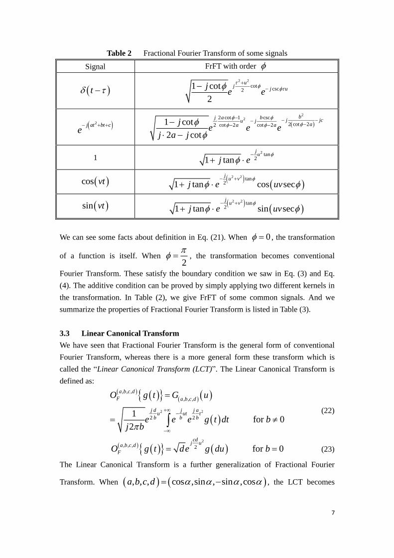
5

where 2in

n e are the eigenvalues of conventional Fourier Transform. Because

the Hermite-Gaussian functions form a complete orthonormal set , we can than

calculate the Fourier Transform by expressing it in terms of these eigenfunctions as

following:

0

n n

n

f x A x

(12)

n nA x f x dx

(13)

2

0

e in

n n

n

f x A x

(14)

The th order Fractional Fourier Transform shares the same eigenfunctions as the

Fourier Transform, but its eigenvalues are the th power of the eigenvalues of the

ordinary Fourier Transform:

2i n

n nx e x (15)

that is, the Fractional operator of order may be defined through its effect on the

eigenfunctions of the conventional Fourier operator.

If we define our operator to be linear, the fractional transform of an arbitrary function

can be expressed as:

2

0

i n

n n

n

f x x A e x

(16)

The definition can be cast in the form of a general linear transformation with kernel

,B x x by insertion of Eq. (13) into Eq. (16):

,f x x B x x f x dx

(17)

0

1 2 2 2

2

0

,

2 exp

2 22 !

n n n

n

i n

n nnn

B x x x x

x x

eH x H x

n

(18)

6

This can be reduced to a simpler form for 0 :

1 2

2 2

ˆexp 4 2,

sin

exp cot 2 csc cot

iB x x

i x xx x

(19)

where 2

and ˆ sgn sin . We see that for 0 and 2 , the

kernel reduces to 0 ,B x x x x and 2 ,B x x x x . These

kernels correspond to the 0th and 2th order Fractional Fourier Transform and as

mentioned we saw the results are f x and f x . Some essential properties are

listed below

1. The Fractional Fourier Transform operator is linear.

2. The first-order transform 1 corresponds to the conventional Fourier transform

and the zeroth-order transform 0 means doing no transform.

3. The fractional operator is additive, .

The kernel of the Fractional Fourier Transform can also be defined in the following

equation:

2 2

cot csc2

1 cotif is not a multiple of

2

, if is a multiple of 2

if + is a multiple of 2

t uj jutj

e

K t u t u

t u

(20)

And the Fractional Fourier Transform is defined by means of the transformation

kernel:

2 2

cot cot csc2 2

1 cotif is not a multiple of

2

if is a multiple of 2

if + is a multiple of 2

,

u tj j jutj

e x t e dt

t

t

X u x t K t u dt

(21)

7

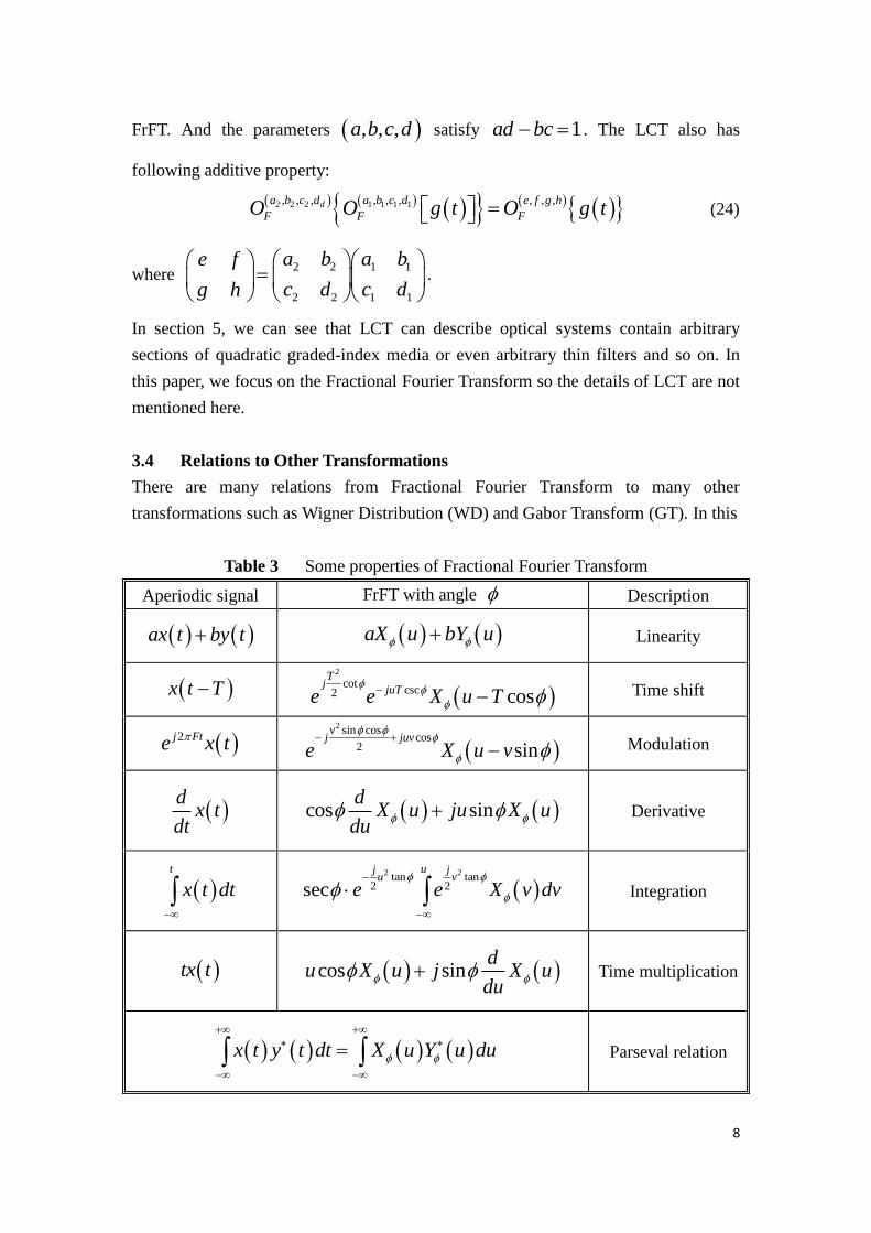
Table 2 Fractional Fourier Transform of some signals

Signal FrFT with order

t

2 2

cotcsc2

1 cot

2

uj

j uje e

2j at bt ce

222 cot 1 csc

2 cot 22 cot 2 cot 21 cot

2 cot

bj a bj jcu j

aa aje e e

j a j

1 2 tan

21 tanju

j e

cos vt

2 2 tan21 tan cos secj

u v

j e uv

sin vt

2 2 tan21 tan sin secj

u v

j e uv

We can see some facts about definition in Eq. (21). When 0 , the transformation

of a function is itself. When 2

, the transformation becomes conventional

Fourier Transform. These satisfy the boundary condition we saw in Eq. (3) and Eq.

(4). The additive condition can be proved by simply applying two different kernels in

the transformation. In Table (2), we give FrFT of some common signals. And we

summarize the properties of Fractional Fourier Transform is listed in Table (3).

3.3 Linear Canonical Transform

We have seen that Fractional Fourier Transform is the general form of conventional

Fourier Transform, whereas there is a more general form these transform which is

called the “Linear Canonical Transform (LCT)”. The Linear Canonical Transform is

defined as:

2 2

, , ,

, , ,

2 21

for 02

a b c d

F a b c d

j d j j au ut t

b b b

O g t G u

e e e g t dt bj b

(22)

2

, , , 2 for 0cd

j ua b c d

FO g t de g du b (23)

The Linear Canonical Transform is a further generalization of Fractional Fourier

Transform. When , , , cos ,sin , sin ,cosa b c d , the LCT becomes

8

FrFT. And the parameters , , ,a b c d satisfy 1ad bc . The LCT also has

following additive property:

2 2 2 1 1 1 1, , , , , , , , ,da b c d a b c d e f g h

F F FO O g t O g t (24)

where 2 2 1 1

2 2 1 1

a b a be f

c d c dg h

.

In section 5, we can see that LCT can describe optical systems contain arbitrary

sections of quadratic graded-index media or even arbitrary thin filters and so on. In

this paper, we focus on the Fractional Fourier Transform so the details of LCT are not

mentioned here.

3.4 Relations to Other Transformations

There are many relations from Fractional Fourier Transform to many other

transformations such as Wigner Distribution (WD) and Gabor Transform (GT). In this

Table 3 Some properties of Fractional Fourier Transform

Aperiodic signal FrFT with angle Description

ax t by t aX u bY u Linearity

x t T 2

cotcsc2 cos

Tj

juTe e X u T

Time shift

2j Fte x t

2 sin coscos

2 sinv

j juv

e X u v

Modulation

d

x tdt

cos sind

X u ju X udu

Derivative

t

x t dt

2 2tan tan

2 2sec

uj ju v

e e X v dv

Integration

tx t cos sind

u X u j X udu

Time multiplication

x t y t dt X u Y u du

Parseval relation

9

section, we introduce some relations between them. These relations are quite

important because many applications are based on them.

3.4.1 Relation to Wigner Distribution

The direct and simple relationship of the Fractional Fourier Transform to the Wigner

Distribution (WD) as well as to certain other phase-space distributions is perhaps its

most important and elegant property.

This property states that performing the th order Fractional Fourier Transform

operation corresponds to rotating the Wigner Distribution by an angle 2

in

the clockwise direction. The Wigner Distribution of a function is defined as:

,

2 2 exp 2

W f x W x v

f x x f x x j vx dx

(25)

,W x v can also be expressed in terms of F v , or indeed as a function of any

fractional transform of f x . There are some properties that are most relevant:

2

,f x W x v dv (26)

2

,F v W x v dx (27)

Total energy ,f x W x v dxdv (28)

Roughly speaking, ,W x v can be interpreted as a function that indicates the

distribution of the signal energy over space and frequency. Now, if ,fW x v denotes

the Wigner Distribution of f x , then the Wigner Distribution of the th order

Fractional Fourier Transform of f x , denoted by ,fW x v

is given by:

, cos sin , sin cosf fW x v W x v x v

(29)

Obviously, the Wigner Distribution of the th order Fractional Fourier Transform

of f x is obtained from ,fW x v by rotating it clockwise by an angle .

10

If we define the rotation operation R for two dimensional functions, corresponding

to a counterclockwise rotation by . Then Eq. (29) can be expressed as:

0W f R W f (30)

Because Fractional Fourier Transform and the rotation operators are additive with

respect to their parameters, we can easily generalize Eq. (30) to:

2 12 1W f R W f (31)

Now, we see Eq. (26) and Eq. (27), these functions can rewrite for the f v :

2

,fW x v dx f v (32)

Eq. (32) can again be rewritten by an operator , which is the Radon transform

evaluated at the angle . The Radon transform of a two-dimensional function is its

projection on an axis making angle with the 0x axis. Eq. (32) rewritten by

Radon transform is:

2

W f f v (33)

3.4.2 Relation to Chirp Transform

We begin this part by considering the following functions and their corresponding

Wigner distributions:

exp 2 ,c cf x j v x W x v v v (34)

,f x x c W x v x c (35)

2

2 1 0

2 1

exp 2 2

,

f x j b x b x b

W x v b x b v

(36)

The first of these results shows that the Wigner Distribution of a pure harmonic is a

line delta along cv v . The second one shows that the Wigner Distribution of a delta

function remains delta function along x c . The third one is chirp function, its

Wigner Distribution is a line delta making an angle 1

2tan b with the x axis.

11

Fig. 1 Wigner distribution of a chirp function

This is shown in Fig. 1.

Recall that in 3.4.1 we saw the effect of Fractional Fourier Transform is to rotate the

Wigner Distribution of a function. Thus we can suspect that a chirp function is the

0 domain representation of pure harmonics or delta function in other fractional

Fourier domains.

Now, by using the kernel in Eq. (19) we have the Fractional Fourier Transform of a

shift delta function 0 0cx x is

1 2

2 2

0 0

ˆexp 4 2

sin

exp cot 2 csc cotc c

jf x

j x x x x

(37)

Here we use 0cx denotes a constant to the 0x axis. For 1 2 , this

reduces to 0exp 2 cj vx , as expected. f x can be considered an

alternative representation of 0 0f x in the th fractional domain. Because

f x is the th order Fractional Fourier Transform of 0 0f x , from last

section, the Wigner Distribution of f x must be a rotated version of which of

0 0f x . This is shown as follows:

0 1 0 1 0, cos sin cW x x x x x (38)

Which we verify that the Wigner Distribution of 0 0cx x is also 0 0cx x

x

v

slope= 2b 1b

12

rotated by . So we can say that a delta function in the th domain,

0cx x , is a chirp function in the th domain.

Now, consider the identity:

0 0 0 0f x f x f x x x dx (39)

and we do the th order Fractional Fourier Transform on both sides, then we

obtain:

0 0f x f x x x dx

(40)

where 0x x is already given in Eq. (37). For special case when 1 ,

that is, the Fourier Transform of 0x x is the pure harmonic

1exp 2 exp 2j x x j fx , which is the kernel of conventional Fourier

Transform.

In fact, the representation of a signal in the th domain is what we call the th

order Fractional Fourier Transform of the signal in 0 (time or space) domain.

But generally, if the representation of a signal in th domain is known, we can find

its representation in the th by taking th order Fractional Fourier

Transform.

As the same in Eq. (39), we can also represent a signal in the th fractional

domain:

f x f x x x dx (41)

or we can represent it as a superposition of harmonics in the 1 th domain:

exp 2f x F v j v x dv (42)

where 1 1 0 1, and F f v x v v x . More generally, Eq. (42) can be

rewritten as the superposition of chirp function in other th domain:

,f x f x B x x dx (43)

where ,B x x is the kernel of th order Fractional Fourier

13

Transform. This is equivalent to finding the projection of f in the th domain

onto the basis function. Note that the representation of these basis functions in the

original th domain is chirp function.

3.4.3 Relation to Gabor Transform

Gabor Transform is one of the time-frequency analysis tools. It is a special case of the

Short-Time Fourier Transform (STFT), where the window function it uses is the

Gaussian function. The Gabor Transform can thus be written by

2( )

( )2 2, 1/2t t

j

fG t e e f d

(44)

If F u is the th order Fractional Fourier Transform of f x , ,fG t is

the Gabor Transform of f x and ,FG u v

is the Gabor Transform of F u .

Then it can be proved that ,fG t and ,FG u v

has the following relation:

, cos sin , sin cosF fG u v G u v u v

(45)

That is, we can find that, like the Wigner Distribution, the Fractional Fourier

Transform of parameter is equivalent to rotating the Gabor Transform in the

clockwise direction with angle . But why we use Gabor Transform instead of using

Wigner Distribution. That is because the Gabor Transform is a linear operator and we

(a)GT of s t (b)GT of r t (c)GT of f t (d)WD of f t

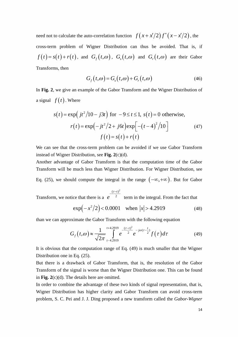
Fig. 2 The Gabor transforms (GTs) and the Wigner distribution (WDs) of s t ,

r t , and f t s t r t . Note that the WDF has the “cross-term problem”

but not the GT.

-10 0 10-10

0

10

-10 0 10-10

0

10

-10 0 10-10

0

10

-10 0 10-10

0

10

14

need not to calculate the auto-correlation function 2 2f x x f x x , the

cross-term problem of Wigner Distribution can thus be avoided. That is, if

f t s t r t , and ,fG t , ,sG t and ,rG t are their Gabor

Transforms, then

, , ,f s rG t G t G t (46)

In Fig. 2, we give an example of the Gabor Transform and the Wigner Distribution of

a signal f t . Where

2

22

exp 10 3 for 9 1, 0 otherwise,

exp 2 6 exp 4 10

s t jt j t t s t

r t jt j t t

f t s t r t

(47)

We can see that the cross-term problem can be avoided if we use Gabor Transform

instead of Wigner Distribution, see Fig. 2(c)(d).

Another advantage of Gabor Transform is that the computation time of the Gabor

Transform will be much less than Wigner Distribution. For Wigner Distribution, see

Eq. (25), we should compute the integral in the range , . But for Gabor

Transform, we notice that there is a

2( )

2

t

e

term in the integral. From the fact that

2exp 2 0.0001 when 4.2919x x (48)

than we can approximate the Gabor Transform with the following equation

24.2919 ( )

( )2 2

4.2919

1,

2

t t tj

f

t

G t e e f d

(49)

It is obvious that the computation range of Eq. (49) is much smaller that the Wigner

Distribution one in Eq. (25).

But there is a drawback of Gabor Transform, that is, the resolution of the Gabor

Transform of the signal is worse than the Wigner Distribution one. This can be found

in Fig. 2(c)(d). The details here are omitted.

In order to combine the advantage of these two kinds of signal representation, that is,

Wigner Distribution has higher clarity and Gabor Transform can avoid cross-term

problem, S. C. Pei and J. J. Ding proposed a new transform called the Gabor-Wigner

15

Transform (GWT). The question now becomes how to combine these two transforms?

We define a new time-frequency transform ,fC t called the Gabor-Wigner

Transform (GWT) that has the following relation with the Gabor Transform

( , )fG t and the Wigner Distribution ( , )fW t

, ( , ), ( , )f f fC t p G t W t (50)

where ,p x y is any function with two variables. It can be proved that ,fC t

also has the rotation relation with the Fractional Fourier Transform. By choosing

appropriate ,p x y , we can achieve our goals of combining the advantages of

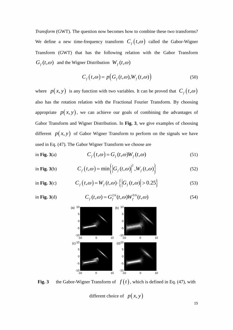
Gabor Transform and Wigner Distribution. In Fig. 3, we give examples of choosing

different ,p x y of Gabor Wigner Transform to perform on the signals we have

used in Eq. (47). The Gabor Wigner Transform we choose are

in Fig. 3(a) , ( , ) ( , )f f fC t G t W t (51)

in Fig. 3(b) 2

, min ( , ) , ( , )f f fC t G t W t (52)

in Fig. 3(c) , ( , ) ( , ) 0.25f f fC t W t G t (53)

in Fig. 3(d) 2.6 0.6( , ) ( , ) ( , )f f fC t G t W t (54)

Fig. 3 the Gabor-Wigner Transform of f t , which is defined in Eq. (47), with

different choice of ,p x y

-10 0 10-10

-5

0

5

10

-10 0 10-10

-5

0

5

10(a) (b)

-10 0 10-10

-5

0

5

10

-10 0 10-10

-5

0

5

10(c) (d)

16

We see that by choosing appropriate Gabor-Wigner Transform, we can have both high

clarity and avoid the cross-term problem.

3.4.4 Relation to Wavelet Transform

The kernels of Fractional Fourier Transform corresponding to different values of

can be regarded as a wavelet family. See the Eq. (19), by the change of variable

secy x , we can write the Fractional Fourier Transform of function f x as:

2 2

2

1 2

exp sinsec

exptan

yg y f C j y

y xj f x dx

(55)

We can take 1 2tan as the scale parameter. And the above equation is the wavelet

transform in which the wavelet family is obtained from the quadratic phase function

2expw x j x by scaling the coordinate and the amplitude by 1 2tan and

C , respectively.

This has recently been shown that the formulation of optical diffraction can be

expressed in a similar wavelet framework. In Chapter 5, we will discuss the filtering

at different Fractional Fourier domains. These operations can also be interpreted as

filtering at the corresponding wavelet transform domain.

3.4.5 Relation to Random Process

In this section, we simply derive the relation between Fractional Fourier Transform

and random process. First, we discuss the relation to stationary random process.

Suppose that g t is a stationary random process, and G u is the Fractional

Fourier Transform of g t . Then we can calculate the autocorrelation function of

G u by applying Eq. (21):

17

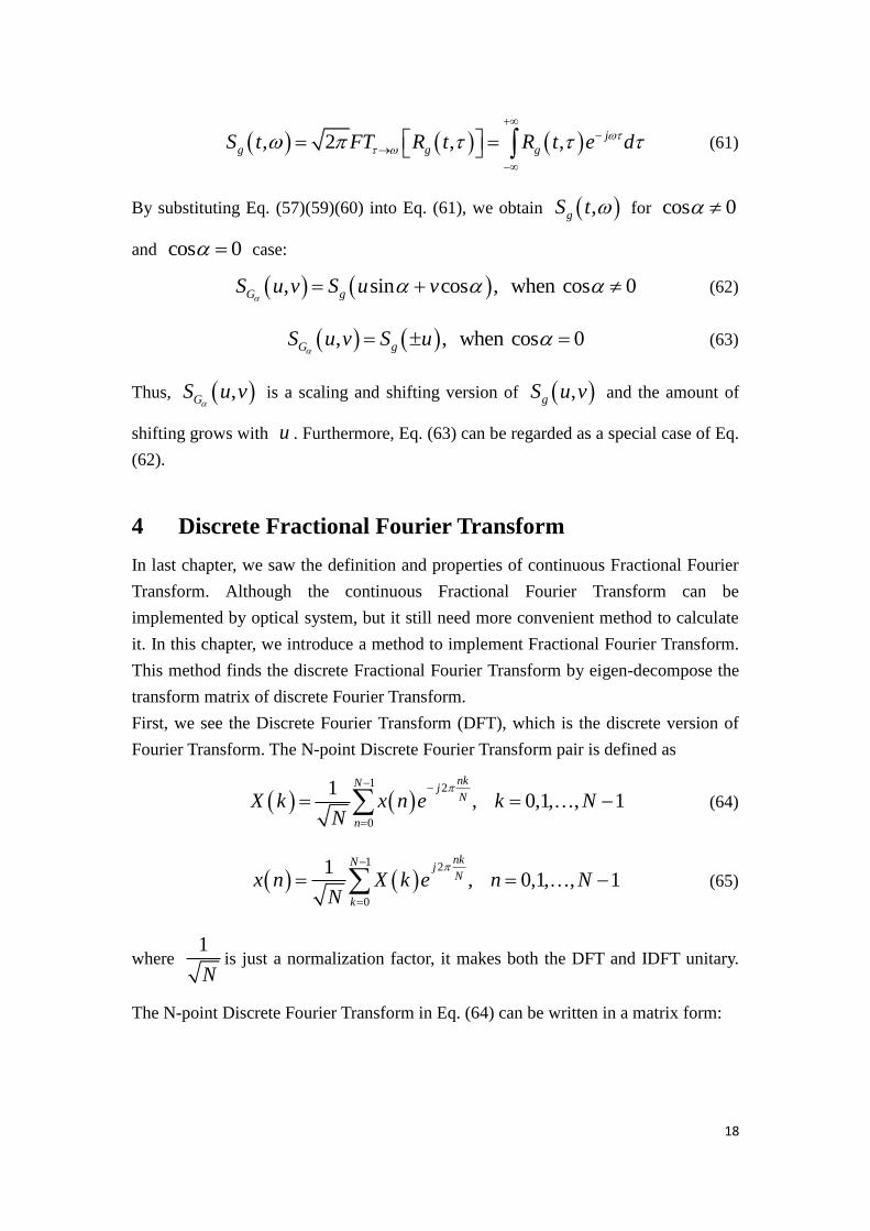
2 2

2 21 1

2 cot2 2 2

2

+ +csc csc cot

2 2 21 1

- -

, 2 2

1+cot=

4

G

ju u

jj u t j u t t t

R u E G u G u

e

e e e E g t g t dtdt

(56)

where 1 1gE g t g t R t t . And by variable changing, Eq. (56) can be

rewritten as

cot

sin cos,cos cos

ujuj

G g

eR u e R

(57)

Although we can see that in Eq. (57), ,GR u

is not stationary. But the amplitude

of ,GR u

is sec secgR . It is independent of u . So we can say that

G u is nearly stationary. Moreover, if g t is real, since GR is also real,

we can thus conclude that

arg , tanGR u u

(58)

So we can use the phase of ,GR u

to estimate the parameter of the

Fractional Fourier Transform.

Now we turn back to Eq. (57), note that this equation is only for cos 0 . For the

case when 1 2K , that is, cos 0 Eq. (57) cannot be applied. So we

get back to Eq. (56) which we applied that csc 1 sin 1 . Then we have

, , when 2 1 2G gR u S u H

(59)

, , when 2 3 2G gR u S u H

(60)

where H is some integer and gS u is the PSD of g t . The definition of

power spectral density of a signal is

18

, 2 , , j

g g gS t FT R t R t e d

(61)

By substituting Eq. (57)(59)(60) into Eq. (61), we obtain ,gS t for cos 0

and cos 0 case:

, sin cos , when cos 0G gS u v S u v

(62)

, , when cos 0G gS u v S u

(63)

Thus, ,GS u v

is a scaling and shifting version of ,gS u v and the amount of

shifting grows with u . Furthermore, Eq. (63) can be regarded as a special case of Eq.

(62).

4 Discrete Fractional Fourier Transform

In last chapter, we saw the definition and properties of continuous Fractional Fourier

Transform. Although the continuous Fractional Fourier Transform can be

implemented by optical system, but it still need more convenient method to calculate

it. In this chapter, we introduce a method to implement Fractional Fourier Transform.

This method finds the discrete Fractional Fourier Transform by eigen-decompose the

transform matrix of discrete Fourier Transform.

First, we see the Discrete Fourier Transform (DFT), which is the discrete version of

Fourier Transform. The N-point Discrete Fourier Transform pair is defined as

1 2

0

1, 0,1, , 1

nkN jN

n

X k x n e k NN

(64)

1 2

0

1, 0,1, , 1

nkN jN

k

x n X k e n NN

(65)

where 1

Nis just a normalization factor, it makes both the DFT and IDFT unitary.

The N-point Discrete Fourier Transform in Eq. (64) can be written in a matrix form:

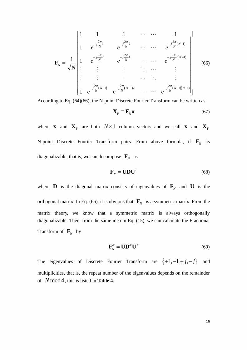
19

2 2 21 2 1

2 2 22 4 2 1

2 2 21 1 2 1 1

1 1 1 1

1

1 1

1

j j j NN N N

j j j NN N N

N

j N j N j N NN N N

e e e

e e e

N

e e e

F

(66)

According to Eq. (64)(66), the N-point Discrete Fourier Transform can be written as

NFX = F x (67)

where x and F

X are both 1N column vectors and we call x and F

X

N-point Discrete Fourier Transform pairs. From above formula, if NF is

diagonalizable, that is, we can decompose NF as

T

N F UDU (68)

where D is the diagonal matrix consists of eigenvalues of NF and U is the

orthogonal matrix. In Eq. (66), it is obvious that NF is a symmetric matrix. From the

matrix theory, we know that a symmetric matrix is always orthogonally

diagonalizable. Then, from the same idea in Eq. (15), we can calculate the Fractional

Transform of NF by

T

N

F UD U (69)

The eigenvalues of Discrete Fourier Transform are 1, 1, ,j j and

multiplicities, that is, the repeat number of the eigenvalues depends on the remainder

of mod4N , this is listed in Table 4.

20

Table 4 eigenvalue multiplicity of DFT matrix

N Mul. Of 1 Mul. Of 1 Mul. Of j Mul. Of j

4m 1m m m 1m

4 1m 1m m m m

4 2m 1m 1m m m

4 3m 1m 1m 1m m

If we let 2 N , and let matrix S

2 1 0 0 1

1 2cos 1 0 0

0 1 2cos 2 0 0

0 0 0 2cos 2 1

1 0 0 1 2cos 1

N

N

S

(70)

It can be easily shown that FS SF . Because S , with distinct eigenvalues,

commutes with F , the eigenvectors of S will be the desired set of eigenvectors of

F . Note that S is a real and symmetric matrix, so its eigenvectors will be real and

orthogonal. Now, we get back to Eq. (69). Because eigenvalues of F are

1, 1, ,j j , it can be written by

11

2 2

1 2 3 4

33

44

0 0 0

0 0 0

0 0 0

0 0 0

T

T

N T

T

j

j

I U

I UF U U U U

UI

UI

(71)

where is the order of discrete Fractional Fourier Transform and iU are given by

1) 1U is constructed by the eigenvectors v of matrix S which satisfy Fv v

2) 2U is constructed by the eigenvectors v of matrix S which satisfy Fv v

3) 3U is constructed by the eigenvectors v of matrix S which satisfy j Fv v

4) 4U is constructed by the eigenvectors v of matrix S which satisfy jFv v

21

5 Applications of Fractional Fourier Transform

A lot of applications of Fractional Fourier Transform have been proposed recently.

Although most of them are the application of the Fractional Fourier Transform to

optical problems, there still have many useful results for signal processing region. In

fact, applications of Fourier Transform may be applications of Fractional Fourier

Transform. In this chapter, I will introduce some applications of Fractional Fourier

Transform such as applications to optical system, applications for filter design,

applications for noise removal and so on.

5.1 Optics Analysis and its Implementation by Fractional Fourier Transform

Both Fractional Fourier Transform and Linear Canonical Transform can be used for

optical system analysis, but when we want to analysis combination of 2 or more

optical systems, it is more convenient to use Linear Canonical Transform. When we

use Linear Canonical Transform, we can use matrices multiplications to analyze the

combination of optical systems. However, if we use Fractional Fourier Transform, we

need to do the integral calculation.

5.1.1 Using FrFT/LCT to Represent Optical Components

a) Propagation through the cylinder lens with focus length f

Suppose the monochromatic light, with wavelength and it has the field

distribution iU x , enters to a cylinder lens with focus length f , thickness ,

and refractive index of . Then from the paraxial approximation, the output will

have the distribution as oU x as

2

2j x

j f

o iU x e e U x

(72)

If we ignore the constant phase, we find it just corresponds to the Linear Canonical

Transform with the parameters

1 0

2 1

a b

c d f

(73)

b) Propagation through the free space (Fresnel Transform) with length z

As the same assumption in a), the relation between input and output distribution when

light propagates through the free space with length z is

22j z

j s xz

o i

eU s e U x dx

j z

(74)

22

This is called the Fresnel Transform. Then, compare with Eq. (22), we find that if the

constant phase is ignored, it corresponds to the Linear Canonical Transform with

parameters as

1 2

0 1

a b z

c d

(75)

Besides a) and b), there are also other optical propagation can be represented by

Linear Canonical Transform.

5.1.2 Using FrFT/LCT to Represent the Optical Systems

According to 5.1.1, since Linear Canonical Transform can represent the 2 optical

operations described above, then we can use Linear Canonical Transform to represent

the optical systems composed of these two operations. We can follow the steps below:

1. For each component in the optical systems, find their parameters of Linear

Canonical Transform. Then each component can be represented by a parameter

matrix.

2. Then calculate the product of the parameter matrices, and we can obtain the

parameters of Linear Canonical Transform for the whole system.

In Fig. 4, we see that if a monochromatic light with wavelength propagate

through a free space with length 0d two lenses with focus length 1f and 2f , it can

be represented by Linear Canonical Transform with parameters as

0

1 2

0 2 0

00 1

1 2 1 2

1 0 1 01 2

2 1 2 10 1

1 2

2 1 11

a b d

f fc d

d f d

dd f

f f f f

(76)

Fig. 4 the implementation of LCT with 2 cylinder lenses and 1 free space

0d

0d

1f 2f

input output

23

Fig. 5 the implementation of LCT with 1 cylinder lens and 2 free spaces

5.1.3 Implementing FrFT/LCT by Optical Systems

By the same concept as 5.1.2, we can also use optical system to implement Linear

Canonical Transform. All the Linear Canonical Transform can be decomposed as the

combination of the chirp multiplication and chirp convolution and we can decompose

the parameter matrix into the following form

1 0 1 01 if 0

1 1 1 10 1

a b bb

d b a bc d

(77)

1 01 1 1 1

if 010 1 0 1

a b a c d cc

c d c

(78)

Thus, for the case that 0b , we can implement Linear Canonical Transform with

two cylinder lenses and one free space as Fig. 4. Similarly, for the case that 0c ,

we can implement Linear Canonical Transform with one cylinder lens and two free

spaces as Fig. 5. And from Eq. (73)(75)(77)(78), we can find the focus length of

lenses and the length of free spaces:

1 0 2

2 2 2for Fig. 4: , ,

1 1

b b bf d f

a d

(79)

0 1 1

2 1 2 12for Fig. 5: , ,

d ad f d

c c c

(80)

Then, the relation between input and output will have the relation as the following

equation

, , ,2exp

a b c d

o F i

Lg x j O g x

(81)

where L is the length of the whole system.

input output

1f

1d

0d

0d

0d

24

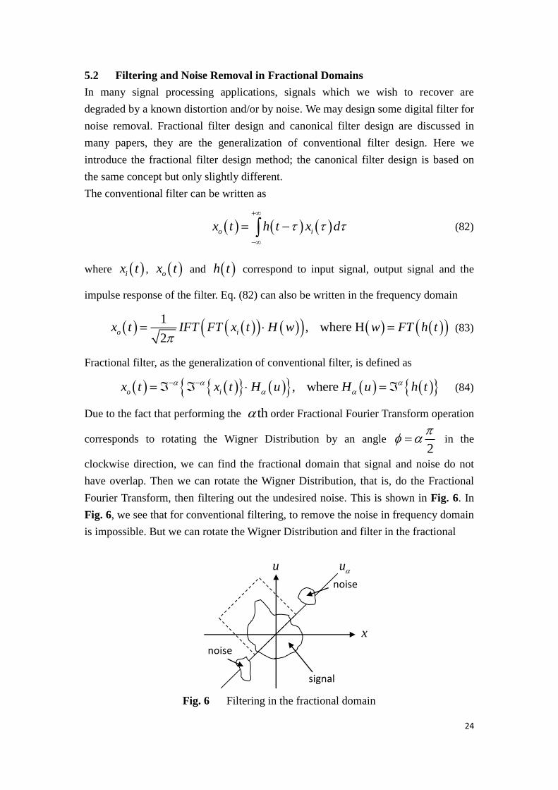
5.2 Filtering and Noise Removal in Fractional Domains

In many signal processing applications, signals which we wish to recover are

degraded by a known distortion and/or by noise. We may design some digital filter for

noise removal. Fractional filter design and canonical filter design are discussed in

many papers, they are the generalization of conventional filter design. Here we

introduce the fractional filter design method; the canonical filter design is based on

the same concept but only slightly different.

The conventional filter can be written as

o ix t h t x d

(82)

where ix t , ox t and h t correspond to input signal, output signal and the

impulse response of the filter. Eq. (82) can also be written in the frequency domain

1

, where H2

o ix t IFT FT x t H w w FT h t

(83)

Fractional filter, as the generalization of conventional filter, is defined as

, where o ix t x t H u H u h t

(84)

Due to the fact that performing the th order Fractional Fourier Transform operation

corresponds to rotating the Wigner Distribution by an angle 2

in the

clockwise direction, we can find the fractional domain that signal and noise do not

have overlap. Then we can rotate the Wigner Distribution, that is, do the Fractional

Fourier Transform, then filtering out the undesired noise. This is shown in Fig. 6. In

Fig. 6, we see that for conventional filtering, to remove the noise in frequency domain

is impossible. But we can rotate the Wigner Distribution and filter in the fractional

Fig. 6 Filtering in the fractional domain

u u

x

signal

noise

noise

25

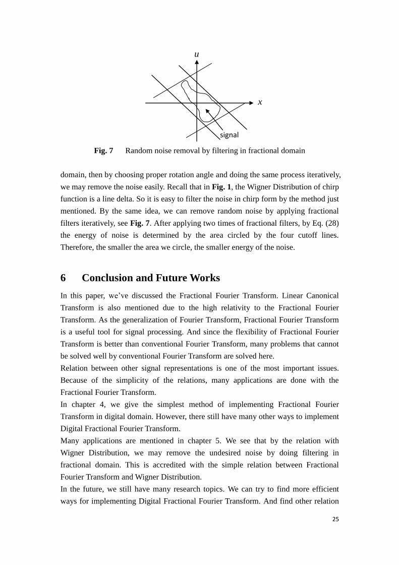
Fig. 7 Random noise removal by filtering in fractional domain

domain, then by choosing proper rotation angle and doing the same process iteratively,

we may remove the noise easily. Recall that in Fig. 1, the Wigner Distribution of chirp

function is a line delta. So it is easy to filter the noise in chirp form by the method just

mentioned. By the same idea, we can remove random noise by applying fractional

filters iteratively, see Fig. 7. After applying two times of fractional filters, by Eq. (28)

the energy of noise is determined by the area circled by the four cutoff lines.

Therefore, the smaller the area we circle, the smaller energy of the noise.

6 Conclusion and Future Works

In this paper, we’ve discussed the Fractional Fourier Transform. Linear Canonical

Transform is also mentioned due to the high relativity to the Fractional Fourier

Transform. As the generalization of Fourier Transform, Fractional Fourier Transform

is a useful tool for signal processing. And since the flexibility of Fractional Fourier

Transform is better than conventional Fourier Transform, many problems that cannot

be solved well by conventional Fourier Transform are solved here.

Relation between other signal representations is one of the most important issues.

Because of the simplicity of the relations, many applications are done with the

Fractional Fourier Transform.

In chapter 4, we give the simplest method of implementing Fractional Fourier

Transform in digital domain. However, there still have many other ways to implement

Digital Fractional Fourier Transform.

Many applications are mentioned in chapter 5. We see that by the relation with

Wigner Distribution, we may remove the undesired noise by doing filtering in

fractional domain. This is accredited with the simple relation between Fractional

Fourier Transform and Wigner Distribution.

In the future, we still have many research topics. We can try to find more efficient

ways for implementing Digital Fractional Fourier Transform. And find other relation

signal

u

x

26

between Fractional Fourier Transform and other signal representation. Moreover, try

to find new applications of Fractional Fourier Transform since most of the

applications now are optical applications.

7 References

[1] Haldun M. Ozaktas and M. Alper Kutay, “Introduction to the Fractional Fourier

Transform and Its Applications,” Advances in Imaging and Electron Physics, vol.

106, pp. 239~286.

[2] V. Namias, “The Fractional Order Fourier Transform and Its Application to

Quantum Mechanics,” J. Inst. Math. Appl., vol. 25, pp. 241-265, 1980.

[3] Luis B. Almeida, “The Fractional Fourier Transform and Time-Frequency

Representations,” IEEE Trans. on Signal Processing, vol. 42, no. 11, November,

1994.

[4] H. M. Ozaktas and D. Mendlovic, “Fourier Transforms of Fractional Order and

Their Optical Implementation,” J. Opt. Soc. Am. A 10, pp. 1875-1881, 1993.

[5] H. M. Ozaktas, B. Barshan, D. Mendlovic, L. Onural, “Convolution, filtering,

and multiplexing in fractional Fourier domains and their relation to chirp and

wavelet transforms,” J. Opt. Soc. Am. A, vol. 11, no. 2, pp. 547-559, Feb. 1994.

[6] A. W. Lohmann, “Image Rotation, Wigner Rotation, and the Fractional Fourier

Transform,” J. Opt. Soc. Am. 10,pp. 2181-2186, 1993.

[7] S. C. Pei and J. J. Ding, “Relations between Gabor Transform and Fractional

Fourier Transforms and Their Applications for Signal Processing,” IEEE Trans.

on Signal Processing, vol. 55, no. 10, pp. 4839-4850, Oct. 2007.

[8] Haldun M. Ozaktas, Zeev Zalevsky, M. Alper Kutay, The fractional Fourier

transform with applications in optics and signal processing, John Wiley & Sons,

2001.

[9] M. A. Kutay, H. M. Ozaktas, O. Arikan, and L. Onural, “Optimal Filter in

Fractional Fourier Domains,” IEEE Trans. Signal Processing, vol. 45, no. 5, pp.

1129-1143, May 1997.

[10] J. J. Ding, “Research of Fractional Fourier Transform and Linear Canonical

Transform,” Doctoral Dissertation, National Taiwan University, 2001.

[11] C. J. Lien, “Fractional Fourier transform and its applications,” National Taiwan

University, June, 1999.

[12] Alan V. Oppenheim, Ronald W. Schafer and John R. Buck, Discrete-Time Signal

Processing, 2nd

Edition, Prentice Hall, 1999.

[13] R. N. Bracewell, The Fourier Transform and Its Applications, 3rd

ed., Boston,

McGraw Hill, 2000.