‘The Formula That Killed Wall Street’?

The Gaussian Copula and the Material

Cultures of Modelling

Donald MacKenzie and Taylor Spears

June 2012

Authors’ address: School of Social & Political Science University of Edinburgh Chrystal Macmillan Building Edinburgh EH8 9LD Scotland email: frances.j.burgess@ed.ac.uk; taylor.spears@ed.ac.uk

2

Abstract This paper presents a predominantly oral-history account of the development of the

Gaussian copula family of models, which are used in finance to estimate the

probability distribution of losses on a pool of loans or bonds, and which were

centrally involved in the credit crisis. The paper draws upon this history to examine

the articulation between two distinct, cross-cutting forms of social patterning in

financial markets: organizations such as banks; and what we call ‘evaluation cultures’,

which are shared sets of material practices, preferences and beliefs found in multiple

organizations. The history of Gaussian copula models throws light on this articulation,

because those models were and are crucial to intra- and inter-organizational co-

ordination, while simultaneously being ‘othered’ by members of a locally dominant

evaluation culture, which we call the ‘culture of no-arbitrage modelling’. The paper

ends with the speculation that all widely-used derivatives models (and indeed the

evaluation cultures in which they are embedded) help to generate inter-organizational

co-ordination, and all that is special in this respect about the Gaussian copula is that

its status as ‘other’ makes this role evident.

3

Given how crucial mathematical models are to financial markets, surprisingly little

research has been devoted to how such models develop and why they develop in the

way that they do. The work on models by researchers on finance influenced by

science studies (work that forms part of the specialism sometimes called ‘social

studies of finance’) has focussed primarily on the ‘performativity’ (Callon 1998 and

2007) of models, in other words on the way in which models are not simply

representations of markets, but interventions in them, part of the way in which

markets are constituted. Models have effects, for example on patterns of prices.

However, vital though that issue is – we return to it at the end of this paper –

exclusive attention to the effects of models occludes the prior question of the

processes shaping how models are constructed and used.

This paper reports research begun by the first author in 2006 on a class of

models known as ‘Gaussian copulas’, which are used in finance to model losses on

pools of loans and to evaluate collateralized debt obligations (CDOs), which are

securities based on pools of debt. (The second author independently began research

in 2009 on the use of similar models by ratings agencies.) The original motivation

was to examine how the Gaussian copula family of models had developed and how

they were used, especially in investment banking. The reason for selecting those

models was that it was already clear in 2006 that (especially via their role in the

evaluation of CDOs) they were of considerable practical importance. In 2007,

however, that original research was overtaken by the outbreak of the credit crisis, a

crisis in which Gaussian copula models were implicated.

4

In February 2009, journalist Felix Salmon wrote that the Gaussian copula had

‘killed Wall Street’ and ‘devastated the global economy’. Its author, ‘math wizard …

David X. Li … won’t be getting [a] Nobel [prize] anytime soon’, wrote Salmon. ‘Li’s

Gaussian copula formula will go down in history as instrumental in causing the

unfathomable losses that brought the world financial system to its knees’ (Salmon 2009).

Although Salmon’s highly personalized focus on Li was, as we shall see, quite misplaced,

he was right to devote attention to Gaussian copulas. Their involvement in the most

serious economic crisis for the better part of a century had the effect of slowing our

research: it made it necessary to set aside our more general work on the history of the

Gaussian copula and concentrate on disentangling its role in the crisis, especially via its

use in rating agencies. With that work now completed (author ref., the findings of which

are briefly summarised in the penultimate section below), we return in this paper to the

original goal of examining the development of the Gaussian copula family of models and

their uses in investment banking.

Fortunately, we are able to control the ‘hindsight bias’ that arises from the

involvement of these models in the crisis by the fact that of the 95 interviews we are

drawing on, 29 took place before the onset of the crisis in July 2007. These 94 interviews

form the primary empirical basis of this paper; also drawn on is the extensive technical

literature on Gaussian copulas. We draw here primarily on the subset of interviews

(numbering 24) that were with ‘quants’, in other words specialists in financial modelling.

Those interviews took a broadly oral-history form: we led each interviewee through those

parts of their career that bore upon the Gaussian copula or similar models and their uses.

Because of the sensitivity of the topic, nearly all the interviews on which we draw have to

remain anonymous. The exception is our interview with the originator of the Gaussian

5

copula family of models, Oldrich Vasicek, conducted in October 2001 as part of an

earlier project (author ref.): given Vasicek’s specific role, anonymity is impossible. We

were unable to interview Salmon’s focus, David X. Li, but were able to put questions to

him by email. As with Vasicek, his role also makes anonymity impossible.

Our analytical focus is on the ‘material cultures’ of modelling.1 Of the two

words, our attention to the material is the more easily explained. Models are not

mathematical abstractions: their use involves material processes. This is the case

even for those models simple enough to be solved by mental arithmetic: the brain,

after all, is a material organ. In fact, though, no member of the Gaussian copula

family is simple enough to be solved in this way, and only one member of the family

(Vasicek’s original model) can be solved using only the mathematician’s traditional

tools of pencil, paper and mathematical tables. All other members require digital

computation, indeed extensive computation. This is not merely an incidental fact

about Gaussian copulas, but an important shaping factor, bearing, for example, on

their use in communication among participants in financial markets. In focussing on

the materiality of models, we are elaborating upon a theme already present in the

social-studies-of-finance literature of models, notably in the emphasis placed by

Beunza and Stark (2004) and Beunza and Muniesa (2005) on the role of the ‘spread

plot’ and other material representations of models, and the discussion by Lépinay

(2011) of their information-technology implementations and their bodily

communication.2

1 Space considerations mean that we focus in this introduction only on previous, broadly science-studies, work on models in finance, and do not attempt to review the wider science-studies literature on modelling, the best introduction to which remains Morgan and Morrison (1999). 2 Lépinay observes: ‘To illustrate problems involving mathematical derivatives, the fingers of each hand come together, and the fingertips of one hand touch the fingertips of the other like two electric

6

Our invocation of ‘cultures’ requires greater elaboration, even though in

invoking ‘culture’ we are following well-established usage in science studies. The

term has been employed there to capture the pervasive finding that scientific practices

(even within the same discipline at the same point in time) are not uniform: there are

different ‘local scientific cultures’ (Barnes, Bloor and Henry, 1996; Bloor 2011),

‘experimental cultures’ (Rheinberger, 1997), ‘epistemic cultures’ (Knorr Cetina,

1999), ‘epistemological cultures’ (Keller, 2002) and ‘evidential cultures’ (Collins,

2004).3 These science-studies usages, however, have – almost unnoticed4 – opened a

gap between our field and some of the connotations of ‘culture’ in the wider social

sciences, where the term is often taken informally to connote ‘issues of meaning,

symbols, values’, and is associated with an implicit theory of action as driven by

matters such as ‘the inescapable weight of habit’ rather than by ‘purposeful tinkering,

strategic aims and interests’.5 To invoke culture, in other words, can too easily be

read as implicitly invoking Garfinkel’s ‘cultural dope’: the person who ‘produces the

stable features of the society by acting in compliance with preestablished and

legitimate alternatives of action that the common culture provides’ (1967: 68).

poles with the same charge, unable to make contact as a result. Hands thus held tense in the shape of a bird’s beak place themselves one above the other and move along an imaginary plane following the movement of a curve. To express the option’s attempt to replicate [see our paper’s second section]… the grouped fingertips follow each other and are adjusted through little jolts’ (2011: 38). 3 Broadly similar invocations of ‘culture’ in the context not of science but of economic life include the ‘cultures of economic calculation’ of Kalthoff (2006) and the ‘calculative cultures’ of Mikes (2009). 4 As far as we are aware, Knorr Cetina (1999: 8-11) is the only published discussion of the relationship of a science-studies usage to wider usages of ‘culture’. 5 The quotations come from two of the three referees of (author ref.). The third referee commented in the similar vein that it was ‘unclear’ why something ‘should be called a “cultural” explanation at all if…turning to this form of evaluation was a perfectly rational thing to do’. Space considerations made it impossible to address those objections in that earlier article (author ref.), which therefore in its published version did not invoke ‘culture’.

7

Science-studies usages of ‘culture’ never invoke cultural dopes. However,

attention to the issue is needed when analyzing modelling, because the cultural dope

has a close relative: what one might call the ‘model dope’, the person who

unthinkingly accepts the outputs of a model. Model dopes are invoked routinely in

public discussion of financial markets, and in seminar presentations we have

encountered audiences utterly convinced that they must exist, indeed that they are

pervasive. However, empirically it is far from clear that model dopes do exist: the

contributions to the nascent social-studies-of-finance literature on modelling that have

addressed the issue have all failed to find them. Mars (1998; see Svetlova, 2012)

shows how securities analysts’ judgements of the value of shares are not driven by

spreadsheet models; rather, they adjust the inputs into these models to fit their ‘feel’

for the ‘story’ about the corporation in question. Svetlova (2009 and 2012) finds

similar flexibility in how models are used: they are ‘creative resources’, she reports,

rather than rules unambiguously determining action. Beunza and Stark find the

traders they study to be ‘[a]ware of the fallibility of their models and far from

reckless’, and fully reflexive: indeed, traders practise ‘reflexive modelling’, in which

models are used to infer others’ beliefs from patterns of prices. This should not

surprise us, point out Beunza and Stark: ‘why should we deny to financial actors the

capacity for reflexivity that we prize and praise in our own profession?’ (Beunza and

Stark, 2010:5).

In our research experience, the ‘model dope’ exists, but not as an actual

person: rather (in the form of, e.g., ‘sheet monkey’ or ‘F9 model monkey’) it is a

8

rhetorical device that actors deploy. 6 It is a way of describing someone as different

from oneself: a way of ‘othering’ them. There is no clear evidence in our research of

model-dope behaviour or beliefs. (For example, none of the 29 interviews we

conducted prior to the crisis contains anything approaching an unequivocal

endorsement of Gaussian copula models.) Any satisfactory notion of ‘culture’, it

seems to us, must treat the cultural dope and its local equivalents such as ‘sheet

monkey’ as forms of othering, not adequate conceptualizations of the actor. Nor are

‘cultures’ equivalent to sets of meanings, symbols and values: they encompass

practices, including the most material of practices. Ultimately, culture should be

treated as a verb, not a noun (it is unfortunate that use of the verb is currently

restricted to its biological sense): people do cultures, rather than culture existing as a

thing causing them to act as they do. Cultural essentialism is similarly quite wrong.

Culture is not a kind of ‘package’ that is ‘coherent inside and different from what is

elsewhere’ (Mol, 2002: 80). All cultures are heterogeneous; all change; all borrow

from elsewhere.

These, however, are very general considerations. The specific cultures within

finance on which we focus – ‘evaluation cultures’, we might call them, given that

determining the economic worth and risks of financial instruments is their core

activity – are at least partially shared sets of practices, preferences, forms of linguistic

or non-linguistic communication, and beliefs (including perhaps an ontology: a

distinctive set of beliefs about what ‘the economic world’ is made of). To count for

us as an evaluation culture, such a set must go beyond the boundaries of any particular 6 ‘Model monkey’ was the pejorative term used by traders in both the Chicago and London options markets to describe other traders who employed printed sheets of theoretical options prices. ‘F9 model monkey’ (Tett 2005) is a similarly pejorative term for a spread-sheet user, and refers to the use of the F9 key to initiate calculation or recalculation.

9

bank or other financial organization. Evaluation cultures ‘cross-cut’ organizations: as

indicated very schematically in figure 1, they are a different form of social

patterning.7 They offer, for example, a route to career advancement complementary to

internal promotions: those who gain a good reputation with their counterparts in other

banks can (very) profitably move. The resultant circulation of personnel, along with

industry meetings, training courses and other mechanisms, often make an evaluation

culture’s practitioners personally known to each other, even in a large financial centre

such as New York or London.8

What follows in this paper is, in part, a story of ‘organization’ trumping

‘culture’: a tale of a family of models that were widely judged inadequate (in

particular by the standards of a ‘locally’ hegemonic evaluation culture), but

nevertheless were – and still are – retained in use, because of the organizational costs

of abandoning them. Those costs, however, are in good part to do with the usefulness

of Gaussian copula models for communication and especially with the patterns of co-

ordinated behaviour that have arisen around the models. Any meaningful concept of

‘culture’, we posit, must view it as a form of and a resource for co-ordinated action,9

and this – we suggest – is the case for evaluation cultures in finance: precisely

because such cultures cross-cut organizations, they facilitate communication and

explicit or implicit co-ordination amongst organizations. For example, it is largely via

7 Figure 1 is of course not to be read too literally. Cultures do not have clear boundaries; nor indeed do organizations (see the delightful parable in Hines, 1988). 8 Beunza and Stark (2004) and Lépinay (2011) discover large differences in practices within the organizations they study, for example differences amongst trading ‘desks’ (subgroups). In our experience, intraorganizational differences of this kind are often manifestations of the intersection of evaluation cultures and organizations: e.g., the practices of the derivatives groups in a bank typically differ greatly from those of its ABS (asset-backed securities) desk, while the practices of the derivatives groups often quite closely resemble those of derivatives groups in other banks. 9 Note that co-ordination does not necessarily imply harmony or the absence of competition: the most bitterly contested football match is still an example of co-ordinated action.

10

evaluation cultures that trading strategies and ideas for trading diffuse amongst

organizations. In our experience (author refs.), what circulates are not fully-fledged

accounts of ideas and strategies but fragments of information (a shouted suggestion to

‘check out what’s going on in Cisco’, a price graph, the information that a well-

regarded hedge fund has bought specific bonds), fragments that make full sense only

to those who to some degree share an evaluation culture, and who will, for instance,

interpret a graph of relative prices in a similar way (see Beunza and Stark, 2010).

Also noteworthy in respect to the role of evaluation cultures in bridging between

organizations is the surprisingly high levels of trust that can exist between apparent

competitors: those in similar roles in other organizations who are pursuing similar

strategies (see Simon, Millo, Kellard and Engel, 2011).

The evaluation culture on which we mainly focus, which we call the culture of

no-arbitrage modelling, is sketched in the second section of this paper. In one

particular local context – the derivatives departments of investment banks – that

culture was and is hegemonic. (A ‘derivative’ is a contract or security the value of

which depends on the price or performance of an underlying asset such as a block of

shares or pool of loans.) We identify that culture’s ontology: it organizes its activities

around a set of probabilities (‘risk-neutral’ or ‘martingale’ probabilities) invisible to

others. We emphasize that culture’s close connections to hedging practices in

derivatives departments (practices utterly central to their work: see Lépinay, 2001),

but also note the presence of aesthetic as well as practical criteria for what counts as a

good model.

11

The third section of the paper describes the early history of the Gaussian

copula family of models. The fourth section of the paper moves to the work of

Salmon’s focus, David X. Li, showing how Li brought to bear an intellectual resource

from a mathematical culture different from that of no-arbitrage modelling (actuarial

science). The section also sketches differences between the two most important

organizational contexts in which Gaussian copulas were used: the credit rating

agencies (Moody’s, Standard & Poor’s and Finch, the focus of author ref.) and the

derivatives department of investment banks, our focus here.

The fifth section of the paper discusses in more detail the embedding of

Gaussian copula models in the practices of investment banking. It shows how the

copula approach mirrored mathematically the relevant organizational structures and

discusses how copula models were used for communication (also highlighting the

limitations in this respect that arose from the materiality of the implementations of the

Gaussian copula). The section goes on to examine the role of the Gaussian copula in

a process that is utterly crucial to the trading of derivatives such as CDOs, which can

involve considerable initial expenses (such as legal costs) but whose maturities

(typically five, seven or ten years) often lie beyond traders’ expected working lives, at

least in their current banks. That process is the achievement of what market

participants call ‘day-one P&L’: the present value of all the expected profit from a

derivative is credited to the trader (e.g., in the calculation of his or her bonus) at the

contract’s inception. (‘P&L’ is the abbreviation of profit and loss.)

The embedding of Gaussian copula models in communication and especially

in the achievement of day-one P&L helps explain the most striking paradox in its

12

history, explored in the paper’s sixth section. In our interviewing, we found that even

some of those who had made the most important technical contributions to the

development of the Gaussian copula family of models rejected those models (one

even denying that they counted as instances of a ‘model’), and that such models

repeatedly failed – not just during the credit crisis but also in an earlier 2005

‘correlation crisis’ – in the sense that a crucial work practice, the calibration of a

model (a term explained below) could not be completed. Nevertheless, Gaussian

copulas were – and are – still used; indeed, they are still canonical. (That paradox is

the methodological key to this entire paper. The very fact that participants do not

generally like Gaussian copulas throws their reasons for using them into clear focus.)

The seventh section then returns to the question posed by Salmon’s article,

enquiring into the extent to which the Gaussian copula family of models ‘killed Wall

Street’. An adequate answer, we posit, demands both a differentiated understanding

of that family of models and also, more importantly, a grasp of the fact that a model

never has effects ‘in itself’ but only via the material cultures and organizational

processes in which it is embedded. The eighth section is the article’s conclusion, and

it ends with the speculation that the role of Gaussian copula models in co-ordination

(manifest here precisely because quants have to give an account of why they keep

using the models despite disliking them) may be a more general phenomenon: that all

shared models in derivatives trading in investment banking are resources for co-

ordinating action.

The culture of no-arbitrage modelling

13

As Kuhn (1970) emphasized, scientific cultures often coalesce around exemplary

achievements. That latter role is played here by the theory of options developed by three

members of the nascent specialism of financial economics, all based in or around MIT:

Fischer Black, Myron Scholes and Robert C. Merton (Black and Scholes 1973; Merton

1973).10

An option is an example of a derivative: it is a contract or security that conveys a

right but not an obligation, for example to buy a set quantity of an underlying asset (such

as a block of shares) at a fixed price (the so-called ‘exercise price’) at a given future time.

One might expect that the price of an option should depend on expectations about

whether the price of the underlying asset is going to rise or fall. On the Black-Scholes-

Merton model, however, that is not so. The price of an option is determined by arbitrage,

in other words by the fact that the prices of two things that are worth the same – that are

entitlements to identical cash flows – must be equal, for if not there is an opportunity for

arbitrage, for riskless profit (one buys the cheaper thing and sells the dearer one, and

pockets the difference).

In developing this ‘no-arbitrage’ model, Black, Scholes and Merton used what

had by the early 1970s become the new specialism’s standard model of share-price

movements: geometric Brownian motion. (Brownian motion is the random movement of

tiny particles, for example of dust and pollen, that results from collisions with the

molecules of the gas or liquid in which they are suspended. The standard mathematical-

physics model of this had been imported into finance, with a simple modification to

10 Space considerations prevent discussion of the intellectual and institutional contexts that gave birth to modern financial economics: see Bernstein (1992), Mehrling (2005) and author ref.

14

remove the possibility of the prices of shares becoming negative, which is an

impossibility because of limited liability: the owners of a corporation’s shares cannot lose

more than their initial investment.) Given geometric Brownian motion and some other

simplifying assumptions (for example of a ‘frictionless’ market, in which both the

underlying asset and riskless bonds can be bought or sold without incurring brokers’ fees

or other transaction costs), Black, Scholes and Merton showed that it was possible to

create a perfect hedge for an option: a position in the underlying asset and in riskless

bonds that, if adjusted appropriately, would have the same payoff as the option whatever

the path followed by the price of the stock, and that furthermore was ‘self-financing’

(once the position was initially established, the necessary continuous adjustments could

be performed without requirement for additional capital). Since they have identical

payoffs, the price of the option must equal the cost of this perfect hedge (or ‘replicating

portfolio’ as it is often called), or else there is an opportunity for arbitrage. That simple

argument determines the price of the option exactly, and nowhere in the formula for that

price is there any reference to investors’ beliefs about whether the price of the underlying

asset was going to rise or fall. Also irrelevant to the price are investors’ preferences or

attitudes to risk (beyond the fact that they prefer more wealth to less), which was a

harbinger of what has become a striking difference between the culture of no-arbitrage

modelling and much of mainstream economics.11

The Black-Scholes-Merton model could have been taken simply as a surprising

result about the pricing of an unimportant security (options were nothing like as

important in the early 1970s as they were later to become). Indeed, that happened: the

11 When learning no-arbitrage modeling from textbooks and courses of the kind discussed below, the second author was struck by the absence of utility functions, a staple of his earlier education in economics.

15

editor of the economics journal in which Black and Scholes’s paper was published

initially rejected it because (as he said in a letter to Black) option pricing was too

specialized a topic (Gordon 1970). However, others within financial economics did

quickly take up and generalize Black, Scholes and Merton’s no-arbitrage model.

Particularly important was the work of Stanford University applied mathematician and

operations researcher, J. Michael Harrison, along with his colleague David M. Kreps and

a former Stanford PhD student, Stanley R. Pliska. Drawing upon ‘Strasbourg’ martingale

theory – an advanced area of probability theory not previously applied to finance – they

proved the two propositions about arbitrage-free, ‘complete’ markets that have become

known as the ‘fundamental theorems of asset pricing’.12

In so doing, Harrison, Kreps and Pliska provided what has become the dominant

mathematical framework in which the exemplary achievement of no-arbitrage modelling,

the Black-Scholes-Merton model, is a special case. Since that framework is at first sight

dauntingly abstract, let us explain some of its salient features using ‘the parable of the

bookmaker’, with which Martin Baxter and Andrew Rennie (quants at Nomura and

Merrill Lynch, respectively) introduced one of the earliest – and still perhaps the most

accessible – textbooks (Baxter and Rennie 1996). Imagine a race between just two horses,

and a bookmaker who knows the true probability of each horse winning: 0.25 for the first

horse, and 0.75 for the second. The bookmaker therefore sets the odds on the first horse

12 First, Harrison, Kreps and Pliska showed that a market is free of arbitrage opportunities if and only if there is an equivalent martingale measure, a way of assigning new, different probabilities (‘martingale’ probabilities) to the path followed by the price of an underlying asset such that the price of the asset (discounted back to the present at the riskless rate of interest) ‘drifts’ neither up nor down over time, and the price of the option or other ‘contingent claim’ on the asset is simply the expected value of its payoff under these probabilities, discounted back to the present. Second, that martingale measure is unique if and only if the market is complete, in other words if the securities that are traded ‘span’ all possible outcomes, allowing all contingent claims (contracts such as options whose payoffs depend on those outcomes) to be hedged with a self-financing replicating portfolio of the type introduced by Black, Scholes and Merton (Harrison and Kreps, 1979; Harrison and Pliska, 1981).

16

at ‘3-1 against’, and on the second at ‘3-1 on’. (Odds of ‘3-1 against’ mean that if a

punter bets $1 and wins, the bookmaker pays out $3 plus the original stake. ‘3-1 on’

means that if a bet of $3 is successful, the bookmaker pays $1 plus the original stake. In

this simplified parable, the adjustments to the odds necessary for the bookmaker to earn a

profit are ignored.)

Imagine, however, that ‘there is a degree of popular sentiment reflected in the bets

made’, for example that $5,000 has been bet on the first horse and $10,000 on the second

(Baxter and Rennie, 1996:1). Over the long run, a bookmaker who knows the true

probabilities of each outcome and sets odds accordingly will break even, no matter how

big the imbalance in money staked, but in any particular race he or she might lose heavily.

There is, however, quite a different strategy available to the bookmaker. He or she can

set odds not according to the actual probabilities but according to the amounts bet on each

horse: in this example, ‘2-1 against’ for the first horse, and ‘2-1 on’ for the second. Then,

‘[w]hichever horse wins, the bookmaker exactly breaks even’ (Baxter and Rennie,

1996:1). As a probability theorist would put it, by adopting this second strategy the

bookmaker has changed ‘the measure’, replacing the actual probabilities of each outcome

(a quarter and three-quarters) with probabilities that ensure no loss (a third and two-

thirds). Those latter probabilities are the analogue of the ‘martingale’ probabilities (see

note 12) invoked by Harrison, Kreps and Pliska.

The shift in measure from actual probabilities to ‘martingale’ probabilities (or

‘risk-neutral’ probabilities, as they are sometimes called) is a pervasive practice – both in

academic financial mathematics and (as discussed below) in the derivatives department of

investment banks – that can reasonably be called the ontology of no-arbitrage modelling.

17

Martingale or risk-neutral probabilities are simultaneously less real and more real than

actual probabilities: less real, in that they do not correspond to the actual probabilities of

events; more real in the sense that (at least in finance) those actual probabilities cannot be

determined, while martingale or risk-neutral probabilities can be calculated from

empirical data, the patterns of market prices. (A bookmaker cannot actually calculate the

true probabilities of the outcomes of a race, but can easily calculate how much punters

have bet with him or her on each horse.) As an interviewee put it, martingale or risk-

mutual probabilities ‘have nothing to do with the past [in other words, they are not based

on the statistical analysis of past events] or the future [they are not the actual probabilities

of events] but are simply the recoding of … prices’.

Socialization into the practices of no-arbitrage modelling was originally quite

localized: at MIT, Robert C. Merton taught a notoriously mathematically demanding

graduate course, described to us by two of his students. More recently, however, such

modelling has become the topic of textbooks such as Baxter and Rennie (1996), Duffie

(1996) or Joshi (2008), and part of the standard curricula of masters courses in

mathematical finance, such as that offered by New York University’s Courant Institute

and Imperial College London. Although such courses are certainly not exclusively

devoted to no-arbitrage modelling, it forms a central part of their curricula. The courses

are expensive (for example, in 2011, tuition fees for the Courant Institute’s degree were

$49,752, and Imperial’s degree cost £24,600),13 but students are willing to pay these large

fees because such courses can lead to well-paying jobs as ‘quants’ (modellers) in the

finance sector.

13 See http://www.quantnet.com/mfe-programs-rankings and http://www3.imperial.ac.uk/pgprospectus. On the practicalities of getting a job as a quant, see Joshi (n.d.).

18

Learning how to do no-arbitrage modelling has become essential for someone

who hopes to become a quant, because there is a rough correspondence between that

modelling and important aspects of financial practices, especially in the derivatives

departments of investment banks. The emphasis on hedging in Lépinay (2011) is

consistent with our interviews: despite the widespread impression of reckless risk-taking

that the credit crisis created, the standard practice of derivatives departments was and is

carefully to hedge their portfolios. Such hedging is incentivized by the way in which

traders are paid (see the discussion below of ‘day-one P&L’), and analyses of the

exposure of derivatives portfolios to the risks of changing prices, changing interest rates,

etc., are part of a daily routine that several interviewees described. The necessary

modelling is very demanding computationally, even when grids of hundreds or thousands

of interconnected computers are devoted to it. So the necessary risk-analysis programs

are typically run overnight, while during the trading day no-arbitrage modelling is applied

primarily in pricing (again, see Lépinay 2011 on ‘pricers’, which are software programs

that run the necessary models). In pricing, all the complication of no-arbitrage modelling

and martingale probabilities reduces to a simple precept: ‘price is determined by hedging

cost’ (McGinty, Beinstein, Ahluwalia and Watts, 2004: 20). It is the strategy of Black-

Scholes-Merton modelling writ large: determine the self-financing, continuously-adjusted

portfolio of more basic securities that will have the same payoff as the derivative,

whatever happens to the price of the underlying asset or assets; use that portfolio to hedge

the derivative; and use the cost of the portfolio as a guide to the price of the derivative.

(In actual practice, of course, the price quoted to an external customer will be greater than

that cost, the difference generating the bank’s profit and the trader’s hoped-for day-one

P&L.)

19

As the overnight computer runs indicate, the practices of hedging and pricing in

investment banking are based not on models as abstractions but on material

implementations. For example, using a model involves the practice that market

participants call ‘calibration’: finding the values of the model’s parameters that are the

best fit to patterns of market prices. Calibration is seldom if ever done ‘by hand’: the

computerized implementation of a model will involve an automatic feed of market prices,

the definition of the criterion of ‘best fit’, and an algorithm that searches for the

parameter values that best fit market prices. Calibration is a crucial part of the daily work

process: if it fails (as it sometimes did during episodes discussed below), it is a crisis for

that work, because automatic ‘pricers’ will not longer function and the appropriate

hedging ratios will no longer be generated.

The critical role of a no-arbitrage model as a guide to hedging generates for

traders a practical criterion of a good model. If they implement the hedges implied by the

model, the profitability of the resultant trading position should be ‘flat’ (constant),

indicating (e.g. to risk controllers) that the position’s risks are being controlled fully.

P&L should not ‘swing too much’, said an interviewee: ‘That is what it is always about’.

Nevertheless, not all judgements amongst models are purely pragmatic. An approach that

can encompass the modelling of a huge range of complex derivatives yet be boiled down

to the two simple theorems formulated by Harrison, Kreps and Pliska fits well with the

preferences for ‘elegance’ of many of those with advanced mathematical training. In the

middle of their textbook, for example, Baxter and Rennie, who have just recast the

derivation of the exemplary achievement, the Black-Scholes-Merton model, in the more

general framework of martingale theory, pause:

20

with a respectable stochastic model for the stock [geometric Brownian motion],

we can replicate any [derivative]. Not something we had any right to expect. …

Something subtle and beautiful really is going on under all the formalism …

Before we push on, stop and admire the view (Baxter and Rennie, 1996: 98).

By now, perhaps, the reader may feel this paper is a badly-telegraphed murder

mystery: the culprit is surely this strange, abstract culture. Not so. The Gaussian copula

family of financial models drew upon resources from that culture, but was never entirely

of that culture. It is time to turn to the history of Gaussian copula.

The origins of the Gaussian copula

The first of the Gaussian copula family of models in finance was developed between

1987 and 1991 by Oldrich Vasicek, a probability theorist and refugee from the Soviet

invasion of Czechoslovakia, who was hired in late 1968 by John McQuown, head of the

Management Science Department of Wells Fargo in San Francisco. McQuown was a

strong supporter of the new field of financial economics, hiring its leading figures such as

Fischer Black and Myron Scholes to work for the bank as consultants, and financing

annual conferences of the field at which Wells Fargo staff members such as Vasicek were

‘able to sit in and listen, wide-mouthed’ (Vasicek interview). Those conferences and his

work for the bank introduced Vasicek to the Black-Scholes-Merton model and to

Merton’s use of stochastic analysis (the theory of stochastic processes in continuous time),

which underpinned the model. In 1983, McQuown persuaded Vasicek (who had left

Wells Fargo to teach finance at the University of Rochester) to join him in a new venture,

a firm called Diversified Corporate Loans. McQuown’s idea was to enable banks to

21

diversify their typically ‘very ill-diversified’ loan portfolios (heavily concentrated in

specific geographical regions or particular industries) by swapping ‘loans that the bank

has on its books for participation shares’ in a much larger, better diversified, pool of loans

originated by many banks (Vasicek interview).

‘[I]t didn’t work’, says Vasicek – banks did not take up the idea – but the

modelling work he did in developing it had lasting effects. In order that the swap could

be negotiated, it was necessary to model the risks of both default on a loan to one specific

corporation and of multiple defaults in a large pool of loans to many corporations.

Financial economists had tackled the first of these problems, but not the second.14 It was

immediately clear to Vasicek that defaults on loans to different corporations could not

plausibly be treated as statistically independent events. As he put it in an unpublished

note, now in his private papers:

The changes in the value of assets among firms in the economy are

correlated, that is, tend to move together. There are factors common to all

firms, such as their dependence on [the] economy in general. Such

common factors affect the asset values of all companies, and consequently

the loss experience on all loans in the portfolio. (Vasicek, 1984: 9)

14 Black, Scholes and Merton – particularly Merton, in what has become known as the Merton or ‘structural’ model of a corporation’s debt (Merton 1974) – had shown how their options model could be applied to modelling the value of corporate debt, via the argument that a corporation’s shareholders in effect own an option on its assets. Imagine, for the sake of simplicity, that the corporation’s borrowing takes the form of a fixed sum (its ‘debt’) that must be paid in full on a given date. If, on that date, the corporation’s assets are worth more than its debt, the aggregate value of its shares is simply the difference between the two. If the assets are worth less than the debt, the shareholders, if economically rational, should allow the corporation to become bankrupt, and the value of its shares is then zero. That payoff structure is exactly the same as that enjoyed by the purchaser of an option to buy the firm’s assets at the fixed price of the firm’s debt (Merton, 1974: 452-54). That was the insight on which Vasicek built his work on the debt of individual corporations, work that eventually became the foundation of a successful company, San-Francisco-based KMV (now owned by the credit rating agency, Moody’s).

22

The task Vasicek set himself, therefore, was to model the value of a pool of loans to

multiple corporations, taking account of the correlation between changes in the values of

different firms’ assets. He was unable to find a general model that had an ‘analytical’

solution: i.e., one that did not involve computer simulation. He did, however, succeed in

formulating an analytically-solvable special case, which has become known as the

Vasicek or large homogeneous pool model.

The special case was a pool of equally-sized loans, all falling due at the same time,

each with the same probability of default, and with the same correlation between the

values of the assets of any pair of borrowers (these features are why the model is referred

to as a ‘homogeneous pool’ model). He showed that as n, the number of loans, becomes

very large the probability distribution of different levels of loss on the portfolio converges

to the expression given as equation 2 of Appendix 1 below, the equation that has been

used to generate Figures 2 and 3 of this paper.

The figures capture a crucial feature of all Gaussian copula models: the radical

differences in the shape of the probability distribution of losses at different correlation

levels. They are based on applying Vasicek’s model to a large pool of homogeneous

loans, each with a default probability of 0.02. (This corresponds roughly to a typical

estimate of the probability of a firm with a low investment-grade rating such as BBB

defaulting in the coming five years.) The expected level of loss on the pool is in all cases

the same in all the graphs: it is just the probability of default on any individual loan, 0.02.

If correlation is very low (e.g., 0.01), the probability distribution of losses on the portfolio

clusters tightly around this expected loss, while if correlation is higher the probability

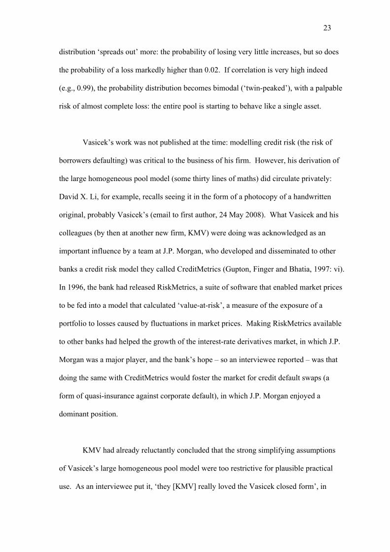
23

distribution ‘spreads out’ more: the probability of losing very little increases, but so does

the probability of a loss markedly higher than 0.02. If correlation is very high indeed

(e.g., 0.99), the probability distribution becomes bimodal (‘twin-peaked’), with a palpable

risk of almost complete loss: the entire pool is starting to behave like a single asset.

Vasicek’s work was not published at the time: modelling credit risk (the risk of

borrowers defaulting) was critical to the business of his firm. However, his derivation of

the large homogeneous pool model (some thirty lines of maths) did circulate privately:

David X. Li, for example, recalls seeing it in the form of a photocopy of a handwritten

original, probably Vasicek’s (email to first author, 24 May 2008). What Vasicek and his

colleagues (by then at another new firm, KMV) were doing was acknowledged as an

important influence by a team at J.P. Morgan, who developed and disseminated to other

banks a credit risk model they called CreditMetrics (Gupton, Finger and Bhatia, 1997: vi).

In 1996, the bank had released RiskMetrics, a suite of software that enabled market prices

to be fed into a model that calculated ‘value-at-risk’, a measure of the exposure of a

portfolio to losses caused by fluctuations in market prices. Making RiskMetrics available

to other banks had helped the growth of the interest-rate derivatives market, in which J.P.

Morgan was a major player, and the bank’s hope – so an interviewee reported – was that

doing the same with CreditMetrics would foster the market for credit default swaps (a

form of quasi-insurance against corporate default), in which J.P. Morgan enjoyed a

dominant position.

KMV had already reluctantly concluded that the strong simplifying assumptions

of Vasicek’s large homogeneous pool model were too restrictive for plausible practical

use. As an interviewee put it, ‘they [KMV] really loved the Vasicek closed form’, in

24

other words a model that yielded an analytical solution, one that could be expressed in the

form of relatively straightforward mathematical expressions (equations 1 and 2 in

Appendix 1). The practicalities of modelling a heterogeneous world meant, however, that

‘they were forced kicking and screaming … to eventually just go with the Monte Carlo’,

as this interviewee put it: in other words, to employ computer simulation. That, too, was

the path taken by the J.P. Morgan team with CreditMetrics. As in other applications of

Monte Carlo modelling (for the history of which see Galison, 1997), random numbers

were used to generate a very large number of ‘scenarios’, and the corporate defaults in

each of the scenarios were aggregated to form an estimate of the loss in that scenario,

with the probability distribution of different levels of loss on the overall pool calculated

by aggregating across all the scenarios. While that sounds very different from Vasicek’s

model with its analytical solution, CreditMetrics employed the same underlying model of

firms’ asset values: correlated geometric Brownian motion. Instead, however, of directly

employing the stochastic differential equations expressing correlated Brownian motion,

as Vasicek had done, CreditMetrics simply used correlated, normally distributed random

numbers to generate the scenarios used in the simulation (Gupton, Finger and Bhatia

1997). It was computationally far more complex, but in a sense conceptually simpler:

CreditMetrics could be understood, at least in outline, by anyone who could grasp the

idea of correlated, normally distributed, random numbers.

Broken hearts and corporate defaults

Both Vasicek’s large homogeneous pool and CreditMetrics were ‘one-period’ models:

even though the underlying stochastic processes took place in continuous time, all that

was modelled was whether corporations defaulted within a single, given time period, and

25

not when in that period they defaulted. It is at this point that David X. Li, the quant on

whom Salmon focuses his article, enters the story. Li was brought up in rural China

(where his family lived because of the Cultural Revolution), and moved to Canada in the

early 1990s for a Masters in Actuarial Science and a PhD in Statistics at the University of

Waterloo. After a session (1994-5) teaching actuarial science and finance at the

University of Manitoba, he became a risk manager at the Royal Bank of Canada and then

a quant in the Canadian Imperial Bank of Commerce, where he modelled ‘credit

derivatives’ such as the CDOs discussed below.

‘I was aware of Vasicek[‘s] work’, Li told the first author in an email message (24

May 2008), and admired its elegance but noted its limitations: ‘I found that was one of

the most beautiful math I had ever seen in practice. But that was a one period

framework’. The yields of a corporation’s bonds, or the prices of the new credit default

swaps, could however be used to model the ‘survival time’ of an individual corporation

(in other words, the time until it defaults). So, as Li put it in this email, ‘the problem

becomes how to specify a joint survival time distribution with marginal distribution [the

probability distribution of the survival time of each individual corporation] given’.

To address this problem, Li drew on a cultural resource not from financial

economics but from actuarial science and ultimately mathematical statistics: copula

functions. While at the University of Manitoba, Li had co-taught with the research

actuary Jacques Carriere. With the sponsorship of the Society of Actuaries, Carriere was

collaborating with Jed Frees of the University of Wisconsin and Frees’s doctoral student

Emiliano Valdez on the problem of the valuation of joint annuities, in particular annuities

26

in which payments would continue to be made to one spouse if the other died (email to

first author from Frees, 23 January 2012).

When pricing joint annuities and calculating the necessary capital reserves,

standard practice in the insurance industry was simply to assume that the deaths of a wife

and of a husband were statistically independent events. That greatly simplified the

calculation: ‘With this assumption, the probability of joint survival is the product of the

probability of survival of each life’ (Frees, Carriere and Valdez, 1996: 230). However, it

was already well-established empirically that there was a tendency for the death of one

spouse to increase the chances of death of the other, a phenomenon ‘often called the

“broken heart” syndrome’ (Frees, Carriere and Valdez, 1996: 230). To help solve the

problem of valuing joint annuities without relying on the assumption of independence,

Frees, Carriere and Valdez drew on work done almost forty years earlier by the Illinois

Institute of Technology mathematician, Abe Sklar. Sklar had introduced the notion of a

‘copula function’, a way of ‘coupling’ a set of marginal distribution functions (in the case

being examined by Frees and his colleagues, the function that specifies the probability

that the wife will die at or before a given age, and the separate function that specifies the

probability that the husband will die at or before another age) to form the ‘joint’ or

‘multivariate’ distribution function (which, in this case, specifies the probability that the

wife will die at or before a given age and the husband will die at or before another age):

see Appendix 2. The work by Frees and his colleagues was both mathematically

impressive (their paper won the 1998 Halmstad Prize of the Actuarial Education and

Research Fund) and of some practical importance: it showed that taking into account the

‘correlation’ between the mortality of a wife and a husband reduced the value of a joint

annuity by around 5 percent (Frees, Carriere and Valdez, 1996: 229).

27

Their work provided Li with the crucial link between his training in actuarial

science and the problems of credit derivatives modelling on which he was working: there

was a clear analogy between a person’s death and a corporation’s default, and the risks of

different corporations defaulting were known to be correlated to some degree, just as the

mortality risks of spouses were. Copula functions permitted Li to escape the limitation to

a single period of the large homogeneous pool model and CreditMetrics (Li, 1999 and

2000), while still drawing a direct connection between his new approach and

CreditMetrics (from January 1999 to March 2000 he worked in the RiskMetrics Group

spun out by J.P. Morgan). Viewed in the lens of Li’s work, the model of correlation in

Vasicek’s large homogeneous pool and in CreditMetrics was a Gaussian copula, in other

words a copula function that couples marginal distributions to form a multivariate normal

distribution function. Although other copula functions were discussed by Li and by

others also exploring the applicability of copula functions to insurance and finance (such

as a group of mathematicians at the Eidgenössische Technische Hochschule Zürich and

University of Zürich with strong links to the financial sector),15 this connection to

CreditMetrics – already a well-established, widely-used model – together with the

Gaussian’s simplicity and familiarity meant that as others took up the copula function

approach, the Gaussian copula had the single most salient role.

From the viewpoint of this paper, the most important modelling problem to which

the Gaussian copula was applied was the evaluation of collateralized debt obligations

(CDOs), securities based originally upon pools of debt instruments such as corporate

15 See Embrechts, McNeil and Straumann (1999), Frey and McNeil (2001) and Frey, McNeil and Nyfeler (2001).

28

bonds or loans to corporations (the somewhat later ABS CDOs, in which the pool

consisted of mortgage-backed securities, will be discussed in the penultimate section of

this paper).16 CDOs became popular from 1997 onwards (see author ref). The firm

(normally a large investment bank) creating a CDO would set up a legally-separate

‘special-purpose vehicle’ (a trust or special-purpose corporation), which would buy a

pool of bonds or loans, raising the money to do so by selling investors securities that were

claims on the cashflow generated from the pool. Crucially, the securities that were sold

were tranched: the lowest, equity tranche bore the first risk of losses caused by default on

the bonds or loans, and only once the holders of that tranche were ‘wiped out’ did losses

impact on the next-highest, mezzanine, tranche (see Figure 4). In a typical CDO, if

correlation was low, then only the holders of the equity tranche would be at substantial

risk of losing their investment. (The greater safety of higher tranches had the downside

that investors in them earned lower ‘spreads’: i.e., lower increments over a baseline

interest rate such as Libor, the London Interbank Offered Rate.) If, however, correlation

was very high (as in the 0.99 case in Figure 3), even the holders of the most senior

tranche were at risk. So modelling correlation was the most crucial problem in CDO

evaluation.

As noted above, Li’s work freed CDO modelling from its restriction to a single

time period. It did not, however, free it from the other chief limitation: that, in practical

problems, no ‘analytical’ solution akin to that of Vasicek’s large homogeneous pool

(equations 1 and 2 in Appendix 1) could be found, so Monte Carlo simulation was needed.

16 Gaussian copula models, especially CreditMetrics, were also used to analyze the risks of banks’ overall portfolios of loans, an application that became particularly important as the simple rules in the 1988 Basel Capital Accord for determining banks’ necessary minimum capital reserves were replaced (under ‘Basel II’) by credit risk models. Although that process of replacement was still not complete by the time of the outbreak of the credit crisis in 2007, it represents another possible connection between the Gaussian copula and the crisis that remains to be researched.

29

The consequences of this were very different in the two main contexts in which the

Gaussian copula was used. In the credit rating agencies – Moody’s, Standard & Poor’s

and Fitch – the task was to work out the probability of default for each tranche of a CDO,

or, in the case of Moody’s, the expected loss on the tranche. (Typically, the constructors

of a CDO aimed to get AAA ratings for the most senior tranches, and BBB ratings or

slightly higher than that for mezzanine tranches.) For working out a probability of

default, a one-period Monte Carlo model akin to CreditMetrics, running on a PC, was

judged perfectly adequate. For example, when Standard & Poor’s introduced such a

model in its new software system, CDO Evaluator, in November 2001, it reported that

the simulation time needed to run a hundred thousand scenarios on a PC was around two

and a half minutes (Bergman 2001). That was not a salient delay: CDOs are complicated

legal and cash-flow structures, and assessing those aspects of them would take far longer

than two minutes. Nor was moving beyond one-period models to Gaussian copulas in

Li’s sense seen in the rating agencies as an urgent priority. Standard & Poor’s made the

move only with version 3.0 of Evaluator, released in December 2005, while Fitch simply

kept using its one-period model, Vector, analyzing a multi-year CDO by running Vector

for the first year and then again for the second year, and so on. (Moody’s also seems to

have stuck with one-period Monte Carlo formulations, although our interviews do not

contain detailed information on practice at Moody’s in this respect.)

The situation in the other main context, investment banking, was quite different.

When CDOs first started to become a relatively large business, in the late 1990s,

evaluating a CDO on a ‘once and for all’ basis (akin to practice at the rating agencies)

was adequate (typically, the risks of all but the equity tranche were sold on to external

parties), and CreditMetrics or similar one-period models were judged up to the job. In

30

the early 2000s, however, new versions of CDOs became popular, of which the most

important were ‘synthetic’ single-tranche CDOs. Instead of consisting of a special-

purpose legal vehicle that bought a pool of debt instruments, these new CDOs were

simply bilateral contracts between an investment bank and a client (such as a more minor

bank or other institutional investor) that mimicked the returns and risks of a CDO tranche.

They became popular because there was heavy demand for the mezzanine tranches of

CDOs, which had an attractive combination of investment-grade credit ratings and

healthy ‘spreads’ (in other words, the ‘coupons’ or interest payments they offered were

set substantially above benchmark interest rates such as Libor). The mezzanine tranches,

however, formed only a small part of the structure of a traditional ‘cash’ CDO of the kind

shown in Figure 4, so mimicking them (without having to tackle the practical and legal

problems of assembling a cash CDO) was an attractive proposition.

The new synthetic single-tranche CDOs were typically constructed and sold by

the derivatives departments of global banks. To the staff in those departments, a single-

tranche CDO, like any derivative, was a product whose risks needed to be hedged, and

indeed it was via that hedging that the bank would make its profits. Unless the tranche

was completely wiped out by defaults on the debt instruments in the hypothetical pool,

the bank kept having to make coupon payments to the investors. To earn money to do so

– and mitigate what from the bank’s viewpoint was the risk of low levels of default – it

could, for example, ‘sell protection’ on (in other words, ‘insure’ against default) each

individual corporation in the pool, in what were becoming relatively well-developed

markets in such protection. Doing so was – very roughly – analogous to hedging an

option, and indeed (with the Black-Scholes-Merton model already familiar to banks’

derivatives departments) the hedge ratios that were needed were christened ‘deltas’.

31

(‘Delta’ is the term used in the options market for the partial derivative – in the calculus

sense of ‘derivative’ – of option value with respect to the price of the underlying asset,

which determines the size of hedge against changes in that price that is needed.) A

single-period CDO model such as CreditMetrics was poorly suited to the task of

determining deltas, so following Li’s work there was rapid, sustained interest in

investment banking in copula formulations.

The delta hedging of single-tranche CDOs and the calculation of other risk

parameters meant that the material constraints on Monte Carlo simulation were a major

issue for investment banks, not the minor one they were for rating agencies. Extracting

reliable estimates of a large set of partial derivatives such as a deltas from a Monte Carlo

copula model was vastly more time-consuming than using the model to price or to rate a

CDO tranche. In a situation in which the IT departments of many big banks were

struggling to meet the computational demands of the overnight runs – ‘some days,

everything is finished at 8 in the morning, some days it’s finished at midday because it

had to be rerun’, an interviewee told the first author in early 2007 – the huge added load

of millions of Monte Carlo scenarios was unwelcome. The requisite computer runs

sometimes even had to be done over weekends: an interviewee told the first author of one

bank at which the Monte Carlo calculation of deltas took over forty hours.

The innovative efforts of investment-bank quants were therefore focussed on

developing what were christened ‘semi-analytical’ versions of the Gaussian and other

copulas. These involved less radical simplifications than Vasicek’s model with its

‘analytical’ solution (equations 1 and 2 in Appendix 1), while being sufficiently tractable

mathematically that full Monte Carlo simulation was not needed and much faster

32

computational techniques such as numerical integration, Fourier transforms and recursion

sufficed. A commonly used simplification was introduced by, amongst others, Jean-Paul

Laurent and Jon Gregory of the French bank BNP Paribas.17 The simplification was to

assume that the correlations amongst the asset values or default times of the corporations

in a CDO’s pool all arose simply from their common dependence on one or more

underlying factors. Most common of all was to assume just one underlying factor, which

could be interpreted as ‘the state of the economy’. The advantage of doing this was that

given a particular value of the underlying factor, defaults by different corporations could

then be treated statistically independent events, simplifying the mathematics and greatly

reducing computation times. By the time Laurent and Gregory published their initially

private May 2001 BNP Paribas paper in the Journal of Risk, they were able to describe

this ‘one-factor Gaussian copula’ as ‘an industry standard’ (Laurent and Gregory, 2005:

2). ‘Factor reduction’ (as this was sometimes called) and other techniques developed by

other quants – such as, for example, the recursion algorithm introduced by the Bank of

America quants Leif Andersen, Jakob Sidenius and Susanta Basu (Andersen, Sidenius

and Basu, 2003) – made it possible for Gaussian copulas, and other copula models, to run

fast enough to be embedded in the hedging and risk management practices of investments

banks’ derivatives departments. Although such techniques might originally have been

proprietary, they quickly became common knowledge amongst investment bank quants.

People moved from bank to bank, carrying knowledge of models with them, and quants –

typically educated to PhD level or beyond – retained something of an academic habitus,

talking about their work to their peers, and seeking opportunities to publish it.

17 Broadly analogous factor models were also discussed at around this time by Rüdiger Frey and Alex McNeil of the Zürich group and Philipp Schönbucher of Bonn University (Frey and McNeil 2001; Schönbucher 2001).

33

Organization, communication and remuneration

CreditMetrics and later semi-analytical versions of the Gaussian copula always had rivals,

but none of them succeeded in displacing them.18 A Gaussian copula model was

relatively straightforward to implement, at least if one was content with a Monte Carlo

implementation such as J.P. Morgan’s CreditMetrics: ‘it was simple and everyone could

build it’, said an interviewee. J.P. Morgan was the dominant bank in the credit

derivatives market (see Tett 2009), and its embrace of Gaussian copulas helped cement

their canonical role: Morgan would simply supply Gaussian models to its clients, and

other investment banks started to do so too. True, the crucial parameters that were

needed in order to use Gaussian copula models, the correlations between the asset values

of pairs of corporations, were extremely difficult to determine: the market value of a

corporation’s assets is not directly observable (accounting conventions mean that it

cannot simply be determined from a firm’s balance sheet, and in any case those balance

sheets are published only quarterly at best). However, the Gaussian copula’s rivals also

had data problems,19 and early users of the Gaussian copula in banks employed a simple

18 Perhaps the most direct rival to CreditMetrics was CreditRisk+ (Credit Suisse First Boston, 1997). Instead of modelling changes in asset value, as CreditMetrics did, CreditRisk+ focussed simply on default, modelling defaults with a Poisson distribution with a variable mean default rate. CreditRisk+ did not explicitly model correlation: instead, the clustering of defaults was modelled via the volatility of default rates. CreditRisk+ had the advantage of not requiring Monte Carlo simulation, and was used reasonably widely by banks to calculate the capital reserves they needed to hold against risks in their loan book, but it does not seem to have been used much in the evaluation of CDOs: ‘CreditRisk+ was developed mostly for non-rated loans held in a “hold to maturity” account. CreditMetrics was developed for a trading situation’ (Nelken, 1999: 237). Credit Suisse also seems to have been less vigorous in promoting it than J.P. Morgan was in relation to CreditMetrics and other Gaussian copula models, with Gupton (2004: 122) commenting about CreditRisk+ that there was a ‘[l]ack of vendor support: Credit Suisse Financial Products does not actively support this as a product’. 19 Supporters of CreditMetrics and CreditRisk+ each criticized the lack of data from which the crucial parameter in the other model could be estimated. Thus Greg Gupton, at that point J.P. Morgan’s CreditMetrics product manager, told journalist Mark Parsley that ‘default-rate volatility measures’, the crucial input into CreditRisk+, ‘will be difficult to obtain because of the lack of default data’. John Chrystal of Credit Suisse Financial Products countered that ‘while correlation data is available for actively traded bonds, a correlation-based approach is not much use if you are looking at a retail loan portfolio with no price history’ (Parsley, 1997: 88).

34

‘fudge’: they used the easily calculated correlation between two corporations’ share

prices as a proxy for the unobservable correlation of the market values of their assets.

A structural feature of the organization of most investment banks also favoured

copula models. Edward Frees and Emiliano Valdez, who with Jacques Carriere had

introduced copula functions to actuarial science, had noted that copulas partitioned the

mathematical task into two separable parts: ‘Copulas offer analysts an intuitively

appealing structure, first for investigating univariate distributions and second for

specifying a dependence structure’ (Frees and Valdez, 1998: 20). The econometric

consequences of splitting the task in this way could be criticized (one interviewee argued

that: ‘if you have, for example, a maximum likelihood estimate of a two-parameter

statistical function then what you should not do is estimate the two parameters in a

sequential way … you will have a bias or a wrong estimate’), but the separation had the

advantage of mirroring how the trading of credit derivatives was usually organized.

Typically, investment banks had one ‘desk’ (trading team) dealing with ‘single-name’

derivatives such as credit default swaps (‘insurance’ against default by a particular

corporation, where the main issue mathematically at stake was a univariate distribution:

its default probability as a function of time) and a separate desk dealing with multi-name

credit derivatives such as CDOs, where mathematically specifying a dependence structure

was necessary.

That the copula approach in this sense mirrored mathematically the relevant

organizational structure was, of course, an advantage of all copula-function models, not

just the Gaussian copula. It was well known to quants that the Gaussian copula had the

unfortunate property of asymptotic ‘tail independence’: as the Zürich mathematicians

35

referred to above put it, ‘Regardless of how high a correlation we choose, if we go far

enough into the tail [the extremes of the distribution] extreme events appear to occur

independently in each margin’, and the Gaussian copula might therefore not ‘be able to

give sufficient weight to scenarios where many joint defaults occur’ (Embrechts, McNeil

and Straumann, 1999: 19; Frey, McNeil and Nyfeler, 2001:1-2). However, while the

Zürich group and others therefore advocated the use of non-Gaussian copula functions,

and such functions were sometimes used in investment banks’ internal modelling, the

Gaussian copula remained canonical, in part because of its use for communication

between banks. If traders in one bank (which for internal purposes used one non-

Gaussian copula) had to ‘talk using a model’ to traders in a different bank that used a

different copula, the Gaussian copula was the most convenient Esperanto: the common

denominator that made communication easy.

In using a model to communicate, an analogy between the Gaussian copula and

the Black-Scholes-Merton model quite consciously influenced participants’ practices.

The latter model could be used not simply to price an option, but to work out the level of

volatility consistent with a given option’s price.20 ‘Implied volatility’, calculated in this

way by running the Black-Scholes-Merton model ‘backwards’, had become a standard

feature of how participants in options markets talked about options, even of how they

negotiated prices. Two traders haggling over the price of an option could talk to each

other not in dollars but in implied volatilities, for example with one trader offering to buy

the option at an implied volatility of 20% and the other offering to sell it at 24%, and

perhaps splitting the difference at 22%.21 Indeed, this practice became sufficiently

20 See Beunza and Stark (2010) for a discussion in a different context of ‘backing out’ a parameter. 21 Other things being equal, the higher the price of an option the higher the implied volatility of the underlying asset.

36

widespread in the options market that prices were, and are, frequently quoted in implied

volatility levels.

A similar communicative practice developed around CDOs, especially from

around 2003-4 onwards, when new markets in what were in effect single-tranche

synthetic CDOs based on a standardized pool of underlying assets were created (the

reasons for their creation are briefly discussed below). These new ‘index’ markets, as

they were called, made ‘market prices’ of CDOs publicly available for the first time

(earlier CDOs had been ad hoc deals privately sold ‘over the counter’ to institutional

investors). They thus offered a new way of inferring correlation, the key parameter of

Gaussian copula models. Instead of trying directly to measure correlation – which was,

as noted, fraught with difficulties22 – a Gaussian copula could be run ‘backwards’ to

extract ‘implied correlation’ (the correlation level consistent with prices in the index

market), just as an options model could be run backwards in order to estimate implied

volatility. To do so necessitated a considerable simplification: the correlations of all pairs

of corporations in the ‘pool’ of the index in question had to be assumed to be identical.

Nevertheless, ‘implied correlation’ became a standard feature of how participants talked

about the ‘index markets’, and to our knowledge when they communicated in this way it

was always a Gaussian copula that was invoked. As in the case of options, the banks that

operated as marketmakers began to quote not just dollar prices but also the corresponding

levels of implied correlation. A quant who had worked on one of these trading desks in

22 After Li’s work, it became increasingly common to formulate models in terms of the correlation of corporation’s survival times, rather than the correlation of the values of their assets, and (in the case of corporations that have not defaulted) survival times are obviously not observable. Hull, Predescu and White (2005) demonstrate that if the conditions of a ‘structural’ model of default akin to Merton (1974) hold, the correlation of two corporations’ survival times is equal to the correlation of the values of their assets.

37

2003-4 told us how he ‘got a lot of pressure from my boss saying … “everyone is asking

me for implied correlation, why aren’t you doing that? You’re terrible.”’

The quant’s reluctance to provide implied correlations reflects the fact that there

were two obstacles to using them for communicating, and only the first was successfully

circumvented. That obstacle was that in the case of many index tranches, especially

mezzanine tranches, running a Gaussian copula model backwards often yielded not a

single correlation value consistent with the ‘spread’ on the tranche, but two values. In

other cases, the model would simply fail to calibrate: it could not reproduce market prices,

and no correlation value would be generated. In a widely circulated critique of existing

practices in respect to ‘implied correlations’ (‘compound correlations’, as they

rechristened them), a group of quants and traders at J.P. Morgan gave an example

concerning mezzanine tranches in one of the main index markets:

… for the traded spread of 227bp [i.e. 2.27% per annum], there are two

possible correlations, one in the 10-15% range, and another around 80%.

Moreover, if the spread on this tranche were over 335bp, there would be

no correlation that gives this spread, and hence no solution (McGinty et al.

2004: 25).

Instead, the J.P. Morgan team advocated that the market move in its communicative

practices from ‘compound correlation’ to what they called ‘base correlation’ (see

Appendix 3). Others in the market quickly saw the advantages of doing so:

communicating using ‘base correlations’ was just as easy, and the practical difficulties of

sometimes having two solutions and sometimes none were almost always avoided. The

38

switch was the final stage in the construction of what, by the time of the first interviews

drawn upon here, was (and still remains, as discussed below) the canonical model: the

Gaussian copula base correlation model.

The second difficulty faced by attempts to communicate – and especially to quote

prices – using correlations proved harder to circumvent, and its roots were again in the

materiality of modelling. Because the Gaussian copula models in practical use were at

best only semi-analytical, different implementations of them could yield different results.

For example, as one interviewee said: ‘There is your [numerical] integration routine. Do

you use a trapezium rule? Do you use Gauss[ian] quadrature? There are all sorts of

nuances.’ As another interviewee put it: ‘What is a single-factor Gaussian copula? …

The implementation is absolutely key. All it [the model] says is, integrate under here.

How you choose to integrate under this function is still open to [different]

implementations. So, yeah, everything will be slightly different.’

The contrast with the Black-Scholes-Merton model was sharp. Its solutions were

in effect fully analytical: sufficiently simple mathematically that different

implementations of them would not lead to results that differed by economically

meaningful amounts. So, for example, two traders could agree a deal ‘priced’ in levels of

implied volatility, and both their models would then output effectively the same dollar

price. With a semi-analytical Gaussian copula, however, two traders could agree on a

correlation level, but even if they were using what was in abstract ‘the same model’, its

different implementations would often produce different prices or spreads, stymieing the

consummation of the deal. As a quant told us in January 2007:

39

… everyone has agreed on this model [Gaussian copula base correlation], but …

let’s say you take two [implementations] built by two different quants. You put in

the same correlations and you might find your CDO price is quite different. … So

if you had 100 basis points [one percentage point] implied spread on a CDO

tranche, you might find that two different models would [output] 99 to 101, and

[the difference] could even be more than that in certain places. So when people

were initially quoting correlation, they found that it didn’t translate into being

tradable, because it still didn’t allow them to pin down the price enough.

In 2004, the J.P. Morgan team that was successfully pushing the idea of base

correlation also tried to tackle this problem of different implementations head on, and

sought to persuade others in the market for standardized indexed tranches all to use

Vasicek’s large homogeneous pool model, with its simple analytical solution (equations 1

and 2 in Appendix 1), as the way to move between correlation levels and prices:

We went out with ... a large-pool model, ‘cos I was hoping it was going to

be Black-Scholes … my hope was, you could almost have it as a quoting

mechanism, right, if everyone had the same model and they all agreed on

the same model it didn’t matter whether it was a good model or not. ...

[W]e could give someone the spreadsheet with it [the large-pool model] in.

So, here you are, there’s no add-ins [additional algorithms such as

implementations of numerical integration] or stuff, ... it’s just standard

sums that you can look into, understand how it works and run it again and

again and again. And we can give that [to market participants].

40

The effort did not succeed. J.P. Morgan’s advocacy of the large homogeneous

pool model for communication and for price quotation was misunderstood as

advocacy of the internal use of the model, for example as a means of calculating

deltas. The misunderstanding was perhaps wilful, because other global banks

were seeking to contest J.P. Morgan’s dominant position in the credit derivatives

market. The effort to achieve communicative consensus around the large-pool

model ‘was fairly successful in Europe’, said an interviewee, but ‘not very

successful in the U.S. where basically our, our sort of rival firms spun it as, “J.P.

Morgan has got an inaccurate model”’. Because the model assumed complete

homogeneity of the assets in a CDO’s pool, it implied exactly the same delta in

respect to each asset, and plainly that was a poor guide to hedging. As another

interviewee put it, market participants ‘all said, “deltas are rubbish”, so they

dropped the model.’

Because J.P. Morgan’s effort did not succeed, the use of the Gaussian

copula for purposes of communication never became as deeply entrenched as the

equivalent use of the Black-Scholes-Merton model in the options market. As an

interviewee said, ‘because the standardized [large homogeneous pool] model

failed, people had to drop correlation as a quotable’ in the standard index tranche

market, a process that was well underway at the time of the first interviews for

this research in 2006. Agreeing deals by agreeing correlation levels did not stop

completely, however, because it provided a point of stability in ad hoc

negotiations, especially amongst sophisticated participants. For example, a

manager of one of the leading hedge funds in this area told us:

41

… you can imagine that if you are having a negotiation with somebody,

and you get to the end of the day, and you can say, ‘I think we got a deal,’

what is it that you have a deal on? … What happens if, when you come in

the next morning, spreads [on the underlying assets] are fifty basis points

wider? … what’s the price? How can we agree that at 5 o’clock today we

are going to make a fair adjustment based on how the market changes for

when we get in tomorrow? Well, we can say, look, spreads are going to

move, dispersion is going to move, let’s just agree on what the implied

correlation is. We agree the implied correlation is 12%, you’re done.

As well as being partially embedded in communication amongst banks and hedge

funds, the Gaussian copula also played a pivotal role in a crucial organizational process:

determining traders’ bonuses. The critical issue here was how and when profit should be

‘booked’. My interviewees reported a universal desire amongst traders for the profits on

a credit derivatives deal (most of which lasted for between five and ten years) to be

recognized in their entirety as soon as the deal was done – as ‘day-one P&L’ – and so to

boost that year’s bonus as much as possible. (‘P&L’ is, as noted, profit and loss, the

crucial determinant of traders’ bonuses.) ‘Let’s say … you sell a deal for … 100 and it’s

really worth 95 [i.e. 95 percent of the sale price]’, said an interviewee. (His example of a

5 percent difference between the price of a deal and its value is probably unrealistically

small. Another interviewee told us that in the early years of the credit derivatives market

it was not unusual for traders to sell a deal ‘at par’ – 100 cents in the dollar – when their

‘bank[‘s] system would have told them that this was worth about 70 cents’. A single

trade ‘would make [$]20 million of P&L.’) Could the difference between price and value

be booked immediately as day-one P&L, or would ‘you have to accrue that profit and you

42

can only take, say it’s a ten-year deal, you can [only] take a tenth each year’? From the

trader’s viewpoint, gradual accrual over ten years was deeply unattractive: most traders

would have left the bank in question well before the ten years were up.

Being able to ‘book’ profit as day-one P&L depended upon having a credible

estimate of value, of how much a deal was ‘really worth’. Up until the bankruptcy of

Enron in 2001, banks had a great deal of discretion concerning whether and how to book

day-one P&L, but because the booking of day-one P&L in energy derivatives played a

significant role in the Enron scandal, the issue began to attract the attention of regulators

and auditors. In 2002, the Emerging Issues Task Force of the US Financial Accounting

Standards Board (FASB) began to examine ‘whether unrealized gains or losses may be

reported at inception of energy trading contracts’ (Emerging Issues Task Force, 2006: 3).

With the Securities and Exchange Commission making clear that the underlying issue did

not affect merely energy derivatives, with concern about the issue growing in Europe as

well, and with the collapse in 2002 of Enron’s auditors, Arthur Andersen, making the

surviving auditing firms aware just how big the dangers were, ‘booking’ moved to centre

stage.

The issue had three main aspects. The first was the observability of the prices or

mathematical parameters used in the calculation of P&L. The FASB’s Emerging Issues

Task Force (2006: 3) concluded that ‘a dealer profit, or unrealized gain or loss at

inception of the contract, may not be recognized unless it is evidenced by quoted market

prices or other current market transactions’. At the start of the 2000s, it would have been

hard credibly to claim that the crucial parameter in Gaussian copula models, correlation,

was observable: it could, at best, be estimated with difficulty. The ‘fudge’ employed in

43

the late 1990s – using the correlations between equity prices (share prices) instead of

correlations between asset values – was too easily contested. As a textbook put it: ‘There

is no theoretical equality between equity correlation and default time correlation. …

[E]quity derived correlations have no theoretical justification’ (Chaplin, 2005: 259-260).

The issue was, interviewees reported to me, a major spur for the development of the

standardized index tranche markets. Correlations ‘backed out’ from market prices in

those markets using a theoretical model were, in practice, agreed by auditors as having

been ‘observed’ from the viewpoint of permitting the booking of profits as day-one P&L.

The second aspect of the issue of ‘booking’ P&L concerns which model to use to

perform this ‘backing out’. Here, the fact that the Gaussian copula base correlation

model was a market standard provided a considerable incentive to keep using it, because

it avoided having to persuade accountants and auditors within the bank and auditors

outside it of the virtues of a different approach. In one bank, we did discover a radically

different model being used instead of a copula, but even there, the model’s developer

told me, ‘finance [i.e. internal accountants and auditors] do look at [Gaussian] base

correlations … for reference’. Furthermore, there was a need to maintain consistency

with the outputs of Gaussian copula models even when one was using a different model.

As this interviewee put it, ‘you have to show that you are matching the market, so that

means that you can match the prices of the … tranches that you see’, prices generally

arrived at by others’ use of the Gaussian copula. Important to this process was and is a

service called Totem, administered by Markit, the leading data provider for credit

derivatives. Each month, Totem sends trading desks a set of hypothetical CDOs to be

priced. The desk quant does the pricing, returns the result to Totem, and receives back

the prices set by all the trading desks using the service. So each bank can assess the

44

closeness of its pricing to the consensus (again, a consensus reached predominantly by

use of the Gaussian copula). ‘You do monthly submissions on [Totem], and as long as

that is showing a happy result [in other words prices close to the consensus] then

finance will be pleased’, said this interviewee.

The third main aspect of achieving day-one P&L was persuading a bank’s risk

controllers that a position was properly hedged and thus that the anticipated profit was

insulated from market fluctuations. The issue here is that deltas and other hedge ratios

are model-dependent. If a trader started to use a model substantially different from the

Gaussian copula, then a position that was properly hedged on that model would not look

properly hedged to risk controllers, unless the trader could succeed in the difficult task

of persuading them to stop using the market-standard model.

The most important role of a correlation model, another quant told the first author

in January 2007, is as ‘a device for being able to book P&L’, and this role sharply

constrained the choice of model available to him:

[Y]ou can’t say, I have the most fantastic model … I love this model and

this model tells me I have made this much money so I want to book this

much profit and pay my traders their bonuses. … You can’t do that, you

have to … to be able to say … I have a hundred-name portfolio which I

traded with a client and I’ve got [a] Gaussian copula base correlation

[model] which is market standard. I fit the model to the market. I then do

all these tricks to price my product, and now it [the model] tells me that I’ve

made x. [That] effectively allows me to do a ten-year trade and book P&L

45

today … without that people would be in serious trouble, all their traders

would leave and go to competitors.

Othering and the crises of the Gaussian copula

From the viewpoint of both communication and remuneration, therefore, the Gaussian

copula was hard to discard. For all its deep entrenchment, however, pervasive

dissatisfaction with the Gaussian copula was expressed by interviewees even in our

earliest interviews in 2006 (including from the quant whose explanation of why the

Gaussian copula had to be used has just been quoted). Indeed, the entire enterprise of

correlation modelling was quite often regarded with some scepticism: one of the leading

hedge funds in credit derivatives had in one of its conference rooms an abacus with the

label ‘Correlation Model’ (Beales 2007).23

One specific source of dissatisfaction with Gaussian copulas was a phenomenon

that market participants christened the ‘correlation skew’. If the Gaussian copula model

were an entirely correct representation, then when one applied it to the different tranches

of a CDO in order to ‘back out’ the implied correlation or base correlation, the correlation

figures that were produced should all be equal. They never were: in particular, the

implied correlation of the highest tranche (sometimes called ‘super-senior’) was always

higher than the correlation implied by the spreads on the mezzanine tranches. So instead

of a ‘flat’ correlation structure, there was a ‘correlation skew’.

23 When the first author visited the fund in May 2009, it had moved offices, and perhaps after the crisis irony no longer seemed appropriate. The abacus was no longer to be seen, but our interviewee confirmed it had been there.

46

There was a closely analogous phenomenon in the pricing of options: the

‘volatility skew’ (indeed, the term ‘correlation skew’ became common currency because

of the analogy). Again, if the Black-Scholes-Merton model were a correct representation,

then the implied volatility of all the options on the same underlying asset with the same

expiration date should be equal. In the early years of the use of the Black-Scholes-

Merton model in options markets, deviations from equality were relatively modest, but

after the 1987 stockmarket crash a systematic volatility skew appeared, and patterns of

prices have never returned to the postulates of the model. Although the topic is complex

(see author ref.), what has in essence happened is that market participants realized after

the 1987 crash that the model underestimated the probabilities of catastrophic events, and

they have adjusted their pricing accordingly.

In options there had thus been a phase (from around 1975 to summer 1987) in

which the Black-Scholes-Merton model was performative in what can be called the

‘Barnesian’ sense: its use helped generate patterns of prices consistent with the model

(see author ref., which invokes Barnes, 1988). The Gaussian copula, in its equivalent

‘pure’ form, never enjoyed an equivalent ‘Barnesian’ phase. The correlation skew

became manifest in 2003-4 with the creation of the market in standardized indexed

tranches, which provided market participants with easily-accessible data from which

implied correlations or base correlations could be backed out using the Gaussian copula.

Even before that, however, ‘in a qualitative sense people knew about the skew’, an

interviewee told us. ‘People knew that the senior tranches had not been priced with the

same correlation as … the junior tranches, because the spread would be like one basis

point [0.01 percent]’. In other words, pricing the most senior tranches using the

correlation level used to price the mezzanine tranches would leave the former with

47

hopelessly unattractive spreads. ‘A lot of this boils down to pretty basic stuff’, said

another interviewee:

Maybe the model says the super-senior tranche only pays [a spread of] three basis

points [0.03 percent], but who the hell is going to read through the whole of the

prospectus, figure out the risk, hire a lawyer to analyze the document, figure out

how to book it, get a model approval, da da da, for something that only pays three

basis points. They’re saying, ‘Look, I’m really not going to get out bed for

anything less than ten [basis] points.’ There is no science in that, it’s just

anything about ten sounds kind of good.

The existence of the correlation skew was not fatal to the use of the Gaussian

copula. In options markets, traders had learned to live with the volatility skew, by

continuing to use Black-Scholes-Merton but employing different inputs for the implied

volatility of options with different exercise prices. This ‘practitioner Black-Scholes’, as it

was sometimes called, might be logically inconsistent, but it was workable. When such

traders moved into credit derivatives, said an interviewee, ‘they were not at all shocked

by this. They said, “well, it just means that there is some kind of implied market …

skew”’. The CDO market proceeded in practice in the same way, using the market-

standard Gaussian copula base correlation model, but with different levels of base

correlation for different tranches. With the exception of the two crises to be discussed

below, that too was a workable way of proceeding. Indeed, as a quant put it to us in a

November 2008 interview, ‘the nice thing’ about the Gaussian copula base correlation

model ‘is that it fits the market exactly, or at least it used to’. (‘Used to’ refers to the

failures of calibration discussed below.) To ‘fit the market exactly’ meant that by using

48

the model with different levels of base correlation for each tranche, it was possible to

‘calibrate’ the model exactly: to find parameters that allowed it to reproduce precisely the

pattern of prices that prevailed in the market.

That quant, however, went on immediately to ‘other’ the Gaussian copula base

correlation model: ‘The bad thing is it’s not a model.’ That statement indicates a second

source of dissatisfaction with the Gaussian copula, at least amongst the quants

interviewed (traders, etc., typically did not give voice to this second source).24 All these

quants were perfectly well aware of the ad hoc fixes that were necessary to keep practices

involving the Black-Scholes-Merton model ‘working’. These, however, were fixes to

what they saw as a good model, indeed the paradigmatic good model: one in which prices

were imposed by arbitrage, and in which there was a well-defined risk-neutral or

martingale measure. The quant who told us that the Gaussian copula was ‘not a model’

went on to explain what he meant: ‘it doesn’t satisfy the law of one price [in other words,

the absence of arbitrage opportunities]. It … can give you inconsistencies and arbitrages

very easily. You’re not computing values … as expectations under some well-defined

measure.’

It is important to note that the quant who said this had made important technical

contributions to the development of the Gaussian copula family of models. Others were

even more critical. ‘Copulas are generally an early doodling activity in an area’, said

another quant in a January 2009 interview. ‘They are a simple trick to allow yourself to

preserve the marginals [default probabilities for individual corporations] and to induce

24 Other sources of dissatisfaction included the Gaussian copula’s asymptotic tail independence (see above) and the fact that copula models had static parameters (e.g., correlation levels that did not change with time).

49

some sort of coupling.’ Copulas ‘are perceived as a hack’, he said, despite having

‘superficially attractive properties like being able to perfectly reproduce markets’.

That these interviews took place in November 2008 and January 2009, after the

credit crisis, may cause the reader to suspect that this othering of the Gaussian copula was

tactical, an attempt by interviewees to distance themselves from it because of its role in

the crisis. However, one of our pre-crisis interviews contained a very similar critique of

the Gaussian copula, again from a quant who had contributed importantly to its technical

development. Right at the start of an interview in January 2007, without any prompting,

he distinguished between the Black-Scholes-Merton model – in which pricing is imposed

by arbitrage and ‘the price is something that is derived from a hedging strategy’ – and the

Gaussian copula, which was, he said, a case in which ‘a pricing model gives everyone a

consensus to all sort of use the same model, put in roughly the same inputs, and therefore

everyone kind of agrees on the same price’:

So, the thing that is very interesting on credit [derivatives] is … almost for

the first time in finance we have models which are not so robust and are

almost there as a kind of consensus, and that’s all very well until

something changes and something can change quite dramatically.

In retrospect, the first author’s thoughts have often gone back to that interview,

some six months before the first unequivocal symptoms of the coming catastrophe. Was

it a warning he missed? The interviewee, however, looked backwards in time for his

example of what he meant, not forwards. In May 2005, just over eighteen months prior

to the interview, the credit derivatives market had been rocked by its first major crisis: the

50

‘correlation crisis’, as market participants came to call it. The ultimate cause of the crisis

was the popularity, noted above, of synthetic single-tranche mezzanine CDOs. The major

banks that marketed these CDOs to their customers ended up buying lots of ‘protection’

(quasi-insurance against default) on mezzanine tranches, which left them with a market

exposure they did not want. That created the possibility of what appeared to be a

mutually beneficial trade between investment banks (saying to themselves, as one

interviewee put it, ‘we can’t have such a concentration of that risk’) and hedge funds,

looking to make profits: salespeople at banks could say to hedge funds ‘I could structure

a trade like this, it’s great value, look at the [price] history’.25

The way the trade worked was that investment banks would reduce their

unwanted exposure by selling hedge funds protection on the mezzanine tranches of

standardized indices similar in their composition to the single-tranche CDOs that the

banks had been marketing. The hedge funds would then sell protection on the lowest

tranches (the ‘equity’ tranches) of those indices, and the income they could earn by doing

so was greater than the expense of buying protection on mezzanine tranches from the

investment banks. By choosing appropriately the relative sizes of the mezzanine

protection bought and equity protection sold, the result was a delta-neutral position (that

is, a position hedged against improvements or deterioration in the perceived overall

creditworthiness of the corporations whose debts underpinned the index in question) that

would nevertheless make a consistent profit for the hedge fund. Even some banks seem

to have been tempted into the trade.

25 The interviewee in question was talking more generally, rather than about the specific trades discussed here.

51

In the terminology of correlation trading, however, the trade made the hedge

funds and banks taking part in it ‘long correlation’: they were exposed to correlation

levels falling. (High levels of correlation benefit those who have sold protection on

equity tranches because it makes outcomes more binary, as in the 0.99 case in figure 2.

The chance of catastrophe sufficiently serious to hit even the most senior tranches

increases, but the chance of little or no loss, and therefore an intact or almost intact equity

tranche, increases as well.) Put another way, the hedge funds were exposed to events that

would provoke concern about idiosyncratic risks; in other words, risks that affect just one

corporation or a very small number of corporations, because such risks endanger the

sellers of protection on equity while leaving the situation of mezzanine tranches almost

unchanged.

Idiosyncratic risk was precisely what manifested itself on 5 May 2005, when

Standard & Poor’s stripped General Motors and Ford of their investment-grade ratings,

reducing GM to BB and Ford to BB+. It was a noteworthy event, a ratings agency

having reduced the obligations of the great mass-market car companies of the 20th

century to ‘junk’. But it took place in generally benign economic conditions: it could

indeed be interpreted as an increase in a very specific risk. What appears then to have

happened, interviewees told us, was that a particular large hedge fund (one interviewee

named it, but it has been impossible to get confirmation of its identity) decided to unwind

its position, which meant buying protection on equity tranches to cancel out its sales. The

cost of ‘protection’ on those tranches thus increased, placing pressure on those who had

similar positions, who then also tried to unwind, further increasing the cost of protection

on equity. In contrast, the cost of protection on mezzanine tranches fell (unwinding

implied having to sell protection on those tranches). When Gaussian copula models were

52

used to ‘back out’ correlation levels, that pattern of change in costs suggested that the

correlation skew had steepened sharply, hence the name ‘correlation crisis’.26

The result, said interviewees, was large losses for a number of hedge funds and

some banks. The crisis attracted very little reporting, either at the time or subsequently,

perhaps because of its complicated nature (and the absence of any spectacular

bankruptcies). The Financial Times reporter Gillian Tett was one of the few to pick up

the story, and the informants she spoke to said that it involved undue faith in models:

‘People thought the models were almost infallible – the last few days have been a real

shock’, one banker told her (Tett 2005). However, when the first author similarly

suggested to another interviewee in January 2007 that the trade had been ‘model-driven’,

he disagreed:

the press always wants to talk about these smart traders who were wrong

because they believed in the models. I mean, no-one is that stupid that

you put on a trade with a delta which is delta-neutral, I mean, no, you

know that it’s only delta-neutral if nothing else changes.

Whatever the role of the Gaussian copula in causing the correlation crisis, it was

certainly something of a crisis for modelling practices. The steepening of the correlation

skew during the crisis was sufficiently large that at some points market-standard

Gaussian copula base correlation models simply failed to calibrate. This was not an

abstract failure, but a material incapacity of models, as implemented in software systems,

26 See the graphs of tranche spreads and the corresponding base correlation levels in early 2005 in Packer and Wooldridge (2005: 6).

53

to be able to find parameter values that allowed the pattern of market prices to be

reproduced. An interviewee reported that this happened both to a particular model he had

developed and more generally:

the [sharply reduced spreads on the] mezzanine tranche actually violated

[the] lower bound that this stochastic correlation model was imposing. …

[The episode] was very upsetting to many people because their models

simply stopped working. They couldn’t match the market any more.

That calibration failure, however, was a failure only on a few particular days, and

the ‘correlation crisis’ did not generate any major widespread change in the dominant

practices of modelling. Far more widespread failures of models to calibrate were,

however, experienced in the second of the crises to afflict correlation modelling, the

credit crisis that erupted in the summer of 2007. As the crisis deepened, the cost of

protection on the apparently safest, super-senior tranches of the indices rose to

unprecedented levels, as fears of systemic collapse increased. It wasn’t, however, simply

that the 0.99 correlation scenario of figure 3 manifested itself in the pattern of market

prices: repeatedly, no correlation value at all could be found that enabled price patterns to

be reproduced. By the autumn of 2007, an interviewee told us, the spreads on super-

senior tranches were so high that the standard implementations of Gaussian copula base

correlation models would not calibrate. In that implementation:

[Y]ou can derive some bounds on the value of the super-senior tranche.

And those bounds were violated by the market. Spreads were too high for

the super-senior tranches. You couldn’t get there.

54

This time, the failure to calibrate was not a transient phenomenon: in 2007-8, repeated

failures of calibration were experienced (for examples, see Brigo, Pallavicini and

Torresetti, 2010: 100).

Hugely disruptive as failures to calibrate are to the day-to-day work of pricing and

hedging, there is nevertheless a sense in which the standard Gaussian copula base

correlation model has survived even this crisis. It has been ‘tinkered with’, rather than

discarded. Prior to the 2007-8 crisis, it was standard to assume that if a corporation

defaulted then the ‘recovery rate’ (the extent to which losses on that corporation’s debts

were less than total) was 40 per cent, which is roughly the historic average. More

recently, however, that assumption has been discarded, and recovery rates have been

modelled as stochastic rather than fixed. In particular, in one-factor Gaussian copula

models, recovery rates have been made dependent upon the value of the underlying factor,

which as noted above can be interpreted as the ‘state of the economy’: it is assumed that

in ‘bad’ states of the economy, recovery rates will be much lower than in ‘good’ states.

Altering the standard model in this way has made it possible for modelling to ‘work’ (to

calibrate) most of the time, even in the very turbulent conditions of recent years.

‘Working’ is still not universal – there have reportedly been particular days when even

with this alteration standard models fail to calibrate (Brigo, Pallavicini and Torresetti,

2010: 104) – but the ‘fix’ has been good enough to keep the Gaussian copula dominant.

Moving to a radically different model would be hard – for the reasons discussed in the

previous section – and in a situation in which the underlying markets have shrunk

dramatically, it is easier to ‘fix’ a model that was already understood by traders and

55

accountants (not just quants) than to suffer the financial, communicative and cognitive

costs of moving to a different approach.

‘The Formula That Killed Wall Street’? What has just been discussed, however, is the (limited) effect of the credit crisis upon

the Gaussian copula family of models. What, however, of the effect in the other

direction? Did the Gaussian copula kill Wall Street?

The actors on which this paper has focussed – the users of Gaussian copula

models in the derivatives departments of investment banks – came under huge strain

(including the calibration failures discussed in the last section), but their activities did

not generate losses of sufficient magnitude to threaten the survival of their banks or of

the financial system. Certainly, there were losses on the credit default swaps, the

index tranches, and the CDOs (based on pools of corporate debt) with which those

actors dealt, but those losses – while very big – were not catastrophic. As an

interviewee said in July 2010: ‘Losses you hear around the place, “I lost a billion

dollars”, which in normal times would be very notable.’ A billion dollar loss,

however, does not kill a big global bank. The level of loss needed to do that (of the

order of $50 billion) did not come from the world discussed here: ‘the base corr guys

[users of Gaussian copula base correlation models] are still standing… There were

definitely bad days for everybody with the markets jerking around, and people felt the

swings but I am not sure that there was anything in terms of an Armageddon for the

models’.

56

Rather, the critical path by which the Gaussian copula was implicated in the

credit crisis was via rating agencies, in particular in the rating not of CDOs based on

pools of corporate debt `but of ‘ABS CDOs’. These are CDOs in which the

underlying assets are asset-backed securities (ABSs), specifically mortgage-backed

securities. These were introduced somewhat later than corporate-debt CDOs, and

originally were a small-scale business: of the 283 CDOs issued in 1997-1999, only

eight were ABS CDOs (Newman et al., 2008: 34, exhibit 1). By the time ABS CDOs

started to become large-scale (from 2001 onwards), the rating agencies already had in

place an organizational division of labour. Both CDOs and ABSs fell within the remit

of their structured finance departments, but those departments had separate groups

rating CDOs, on the one hand, and ABSs on the other (author ref.).

The new ABS CDOs were therefore evaluated by the rating agencies in two

temporally and organizationally separate steps. First, the underlying mortgage-backed

securities or other ABSs were rated by the groups handling ABSs, and then the

overall CDO structure was rated by the CDO groups. Instead of considering ABS

CDOs as radically different instruments that required an altogether new form of

evaluation, the CDO groups simply made relatively modest modifications to their

existing techniques for analyzing CDOs with pools consisting of corporate debt. From

late 2001 onwards, those techniques increasingly involved the use of models in the

Gaussian copula family, albeit – as noted above – usually one-period models

analogous to CreditMetrics, not fully-fledged copulas of the kind introduced by Li.

With little econometric data to draw upon (empirically estimating the correlation

between ABSs is an even harder econometric problem that estimating corporate

correlations), the CDO groups employed largely judgment-based ABS correlation

57

estimates broadly similar to those they used for the analysis of corporate CDOs. When,

for example, Standard & Poor’s introduced its new one-period Gaussian copula

system, CDO Evaluator, in November 2001 the same correlation (0.3) was used for

the correlation between ABSs from the same sector (for example, ABSs based on

subprime mortgages) as was used for the correlation between corporations in the same

industry (Bergman 2001).

The result of the assumption of only modest correlation was an extremely

attractive opportunity for market participants to take ABSs of only modest credit

quality (for example, the mezzanine tranches of mortgage-backed securities with BBB

ratings) and package them into CDOs with very large AAA tranches. Widespread

exploitation of this opportunity had catastrophic consequences, both direct and

indirect. A substantial proportion of the gigantic losses that directly crippled global

financial institutions were incurred in ABS CDOs,27 and the avid demand of ABS

CDOs for the mezzanine tranches of subprime mortgage backed securities also had

the indirect effect of side-lining the traditional buyers of such securities, who had

typically scrutinized the underlying pools of mortgages with great care (Adelson and

Jacob, 2008a). ABS CDOs sat at the end of what market participants sometimes call

an ‘assembly line’, in which subprime mortgages were bundled into ABSs, and then

ABSs were bundled into ABS CDOs, with a view simply to achieving desirable

ratings with little effective concern for risks in the underlying assets that were not

captured by those ratings.

27 Citigroup lost $34 billion on ABS CDOs, Merrill Lynch $26 billion, UBS $22 billion and AIG $33 billion (Benmelech and Dlugosz, 2009).

58

In effect, market participants had ‘outsourced’ the analysis of ABS CDOs to

the rating agencies. It was perfectly possible to profitably construct an ABS CDO

without doing any correlation analysis of one’s own: all one had to do was to check

that an intended structure would achieve the desired large AAA tranches, a task that

was made easy by the fact that market participants could simply download Standard

& Poor’s CDO Evaluator and its analogues at the other agencies. The first author

vividly remembers a February 2009 interview in which he asked a senior figure at a

firm that managed ABS CDOs what correlation model the firm had employed, only to

be met with a blank stare: no model of its own had been used.

In the major investment banks, some analysis of ABS CDOs (beyond simply

checking desired ratings) was conducted, but in most cases very little by the standards

of the culture of no-arbitrage modelling. ABS CDOs often fell outside the remit of

the derivatives departments of those banks. They were frequently constructed and

analyzed by other groups, such as those specializing in mortgage-backed securities:

‘The guys doing ABS had essentially different roles and different attitudes’, reported

one interviewee. With one partial exception, Goldman Sachs, such modelling of ABS

CDOs as was done did not take the form of no-arbitrage modelling.28 Rather, it

involved either cashflow models of the underlying ABSs (with judgment-based

estimates of likely mortgage default rates) fed into a cashflow model of the CDO, or

inferring the default probabilities of the ABSs from their ratings and using them in a

28 Goldman’s modelling of ABS CDOs used estimates of default probabilities and correlations based on patterns of market prices, not, e.g., the historical records of mortgage defaults used by other banks and by the rating agencies. Our hypothesis is that this may in part account for Goldman’s decision to exit the subprime market (and indeed to ‘short’ it) as conditions began to deteriorate late in 2006, a decision that made it possible for Goldman to survive the crisis financially almost unscathed. However, the lawsuits currently faced by Goldman make it impossible for us to interview those involved.

59

Gaussian copula model of the CDO, in much the same way as the rating agencies

modelled ABS CDOs. To those whose view was that the proper activity of a quant

was no-arbitrage modelling, the catastrophic losses were thus on products (ABS

CDOs) that in the words of one such quant ‘were on the whole either less quanted or

not quanted at all’.

An issue of ontology underlies judgements such as that made by the

interviewee just quoted. As noted, no-arbitrage modelling extracts martingale or risk-

neutral probabilities from patterns of market prices. Goldman aside, this style of

modelling – which is what the interviewee meant by ‘quanting’ – was, as far as we

can discover, simply not applied to ABS CDOs. Rating agencies did model ABS

CDOs, but rating agencies do not work with martingale probabilities: rather, they seek

to estimate actual probabilities of default, and to do so they use the historical records

of defaults, not price patterns.29 In the case of subprime mortgage-backed securities,

which dated at most only from the 1990s, such records encompassed only one

relatively mild recession and almost continuously rising house prices. Unfortunately

– as we now know only too well – when those conditions changed, such securities,

and the mortgage borrowers on whom they were based, began to behave quite

differently.

Conclusion

29 In 2002, Moody’s bought Vasicek’s firm, KMV. The acquisition seems, however, not to have brought about a major change in how Moody’s rated CDOs.

60

As the previous section has outlined, the Gaussian copula family of models was

implicated in the processes that ‘killed Wall Street’. Salmon, however, is quite wrong

to focus on David Li. By the time of the crisis, the ratings agencies had moved only

partially from the early one-period models to fully fledged copula models of the kind

introduced by Li, and the move was not of great consequence to the processes

generating the crisis. It was far less consequential than the way in which the

evaluation of ABS CDOs was mapped onto the organizational structure of the

agencies (the separate analyses of first the component ABSs and then the CDO’s

structure), the estimation of the probabilities of default on ABSs using data from a

period of benign economic conditions, and the fact that the CDO groups in the

agencies analyzed an ABS CDO in almost the same way as a CDO based on corporate

debt.

Nor would it be reasonable to blame the Gaussian copula family of models, in

itself, for the crisis. These models did not have unitary, intrinsic effects: they had

effects only in combination with the material cultures in which they were

implemented and organizational processes in which they were embedded. Gaussian

copula models as employed by the rating agencies were different in their effects from

Gaussian models employed in the derivatives departments of investment banks. Not

only were the goals and the ontology different (the rating agencies sought to estimate

actual probabilities of default; the banks sought to extract risk-neutral probabilities

and hedging ratios), but the surrounding processes also differed. Governance (risk

control and the booking of profit) was certainly one aspect of the use of the Gaussian

copula in investment banks, but ratings were almost entirely about governance. With

many investment managers constrained either by regulation or by organizational

61

mandate to buy only investment-grade securities, the ratings of such securities

dictated the nature of the market for them.

The result of the embedding of Gaussian copula models in governance via

ratings was the large-scale ‘gaming’ of them and of the other models employed by the

ratings agencies. The crisis was caused not by ‘model dopes’, but by creative,

resourceful, well-informed and reflexive actors quite consciously exploiting the role

of models in governance. ‘[T]he whole market is rating-agency-driven at some level’,

one of our earliest interviewees told us, a year before the crisis: ‘the game is …to

create …tranches which are single-, double- or triple-A rated, and yield significantly

more than a correspondingly rated [bond]’. That interviewee did not himself directly

participate in that ‘game’ (his hedge fund was profiting only indirectly from the fact

that, as he put it, ‘there are investors who are constrained by ratings’), but other

interviewees did. Two told us how they had employed optimization programs to find

the highest-yielding pools of securities that would still make possible CDOs with

sufficiently large AAA tranches (although they did not directly say this, the highest-

yielding securities are those that market participants consider riskiest). A third

interviewee reported that there were companies that discreetly sold software packages

designed to perform this fatal optimization.

Two dangers, however, attend the above conclusions. First, our emphasis on

knowledgeable, reflexive actors rather than model dopes could be read as a collapse

into simplistic rational-actor, agency-theoretic explanations of the crisis. That is quite

the opposite of our intention. Culture and rationality are not opposed, even if

rationality is construed as the pursuit of narrow self-interest. Even the most selfishly

62

rational actor needs to calculate what is in his or her best interest, and that calculation,

we posit, of necessity partakes in the material cultures of finance. Because those

cultures differ, and because there is no a priori way to be sure which practices are the

most efficacious, even the most reflexive, rational actor cannot stand wholly outside

of finance’s cultures of evaluation. Nor does the existence of such actors diminish the

coordinating role of models or other cultural resources. The way in which Gaussian

copulas, a class of model that was widely disliked, nevertheless helped achieve

economically crucial outcomes (in particular the achievement of day-one P&L) shows

that cultural resources can co-ordinate action even in the presence of widespread

scepticism as to their worth. One does not need to invoke cultural dopes to

understand how cultural resources help produce co-ordinated action.30

The second danger is that this paper’s findings will be read as an endorsement

of no-arbitrage modelling, one of the hegemonic cultures of modern finance. That is

emphatically not our intention. Rather, what we would note is that there are multiple

mechanisms of counterperformativity, in other words multiple ways in which the

practical use of a model can undermine its empirical adequacy.31 One such

mechanism was primary in the credit crisis: the way in which the use by the rating

agencies of Gaussian copula models with low default probabilities for mortgage-

30 For a broader statement of this view of social order, see Barnes (1995). 31 Of course, not all danger comes via counterperformativity, and a specific danger of hedging – the distinctive form of trading associated with no-arbitrage modelling – is that because those who practise it are seen as mitigating risks, they may be able to build up positions that are much larger (and thus actually more dangerous) than those of traders who explicitly take on ‘directional’ risks. A possible example may be ‘the London whale’, the J.P. Morgan credit-derivatives index trader who seems to have lost his bank $2 billion via huge sales of protection on the most active series of the most important North American corporate credit derivatives index, the CDX.NA.IG. These sales seem to have been motivated by hedging, but at the time of writing (18 May 2012) the exact nature of the ‘short’ position (purchases of protection) being hedged is unclear. The very difficulty of identifying what was being hedged indicates a further issue: a ‘hedge’ is not a self-evident feature of the world, but a contestable cultural category.

63

backed securities and only modest correlations among those securities helped create

(via the ‘gaming’ of those models) an outcome that involved huge levels of highly-

correlated default. But there are others. In particular, no-arbitrage models may be

associated with a distinctive mechanism of counterperformativity, in which the

hedging practices those models demand have effects on the market for the underlying

assets that undermine the empirical adequacy of the views of asset-price dynamics

embedded in those models. The most obvious such case is the 1987 stock market

crash, in which portfolio insurance (a form of hedging inspired by the paradigmatic

no-arbitrage model, Black-Scholes-Merton) was at least to some degree implicated in

violent price movements that were grotesquely unlikely on the geometric Brownian

motion model underpinning Black-Scholes-Merton (author ref). Almost certainly,

further research will reveal other instances of this mechanism.32 It could be that here

we have the beginnings of a typology of mechanisms of counterperformativity:

models used for governance are undermined by being gamed; models used to hedge

derivatives are undermined by the effects of that hedging on the market for the

underlying asset.33

32 If the amount in the previous note of the ‘whale’s’ trading is correct, it had an aspect of this kind, in that it led the prices of the CDX.NA.IG to ‘decouple’ from what all models would suggest is a crucial determinant of those prices, the costs of credit default swaps on the corporations making up the index’s pool. Another example comes from the interviewee quoted in the previous section who told us that the credit crisis was not ‘an Armageddon’ for the Gaussian copula base correlation models of CDOs. He immediately went on to tell us of a huge disruption – quite unreported in the press, even the financial press – that had taken place in the interest rate market and had been caused by the hedging of interest-rate derivatives: ‘There were chunky losses all around the City, and that was essentially a model failure in that the model didn’t say that [the change in price patterns that took place] could happen.’ 33 We thank David Stark for pressing on us the importance of a more systematic understanding of counterperformativity. A third form (not found in the episodes discussed here) is what might one might call ‘deliberate counterperformativity’: the employment of a model that one knows overestimates the probability of ‘bad’ events, with a view to reducing the likelihood of those events (for an example, see author ref).

64

We end, however, with a speculation about the culture on which we have

focused, no-arbitrage modelling. As this paper has shown, the canonical Gaussian

copula base correlation model played a co-ordinating role within and among

investment banks: harmonizing practices and prices; at least to some extent

facilitating communication; providing a shared yardstick that enabled accountants and

auditors to determine whether a valuation was correct and risk managers to assess

whether a position was properly hedged; and – therefore – permitting day one P&L,

the essential lubricant of the trading of derivatives with maturity dates that stretch

beyond traders’ likely working lives in their banks. This co-ordinating role of the

Gaussian copula was visible to our interviewees – and therefore to us – precisely

because they did not ‘naturalize’ the model: no-one believed that the Gaussian copula

gave a faithful account of the economic world. Perhaps, though, that co-ordinating

role is ever-present in shared models in finance, even those that are taken as capturing

at least some aspects of the way the world is. Perhaps the modelling of derivatives in

investment banking always has an aspect of what one of our interviewees memorably

called a ‘ballet’, in which highly-paid quants are needed not just to try to capture the

way the world is, but also to secure co-ordinated action. Perhaps the quant is actually

a dancer, and the dance succeeds when the dancers co-ordinate. But – as Beunza and

Stark (2010) have suggested in a different context – perhaps the seeds of disaster

sometimes lie in that very success.

65

Appendix 1: Vasicek’s Large Homogeneous Pool Model

Vasicek applied to firms’ asset values what had become the standard geometric Brownian

motion model. Expressed as a stochastic differential equation,

iiiiii dzAdtAdA σµ +=

where Ai is the value of the ith firm’s assets, µi and σi are the drift rate and volatility of

that value, and zi is a Wiener process or Brownian notion, i.e. a random walk in

continuous time in which the change over any finite time period is normally distributed

with mean zero and variance equal to the length of the period, and changes in separate

time periods are independent of each other.

In Vasicek (1987 and 1991), he considered a portfolio of n equally-sized loans,

to n such corporations, with each loan falling due at the same time and each with the

same probability of default p. Making the assumption that the correlation, ρ, between

the values of the assets of any pair of borrowers was the same, Vasicek showed that in

the limit in which n becomes very large, the distribution function of L, the proportion

of the loans that suffer default, is

€

P[L ≤ x] = N 1− ρN−1(x)− N−1(p)ρ

%

& '

(

) * ... (1)

where N is the distribution function of a standardized normal distribution with zero

mean and unit standard deviation. The corresponding probability density function is:

⎟⎟⎠

⎞⎜⎜⎝

⎛+−−−

−= −−− 21211 ))((

21))()(1(

21exp1)( xNpNxNxf ρρρ

ρ ...(2)

66

(Figures 2 and 3 show graphs of this function with p = 0.02 and four different values

of ρ.) Vasicek went on to show that the assumption of equally-sized loans was not

necessary, and that this limit result still held so long as

€

wii= 1

n

∑ 2 tended to zero as n

became infinitely large, where wi is the proportion of the portfolio made up of loan i.

‘In other words, if the portfolio contains a sufficiently large number of loans without

it being dominated by few loans much larger than the rest, the limiting distribution

provides a good approximation for the portfolio loss’ (Vasicek, 2002: 160-1).

67

Appendix 2: ‘Broken Heart’ Syndrome and a Bivariate Copula Function Let X be the age at death of a woman and Y the age at death of her husband. In the

notation of Frees, Carriere and Valdez (1996), let H(x,y) be the joint distribution

function of X and Y: i.e. H(x,y) is the probability that the wife dies at or before age x,

and that the husband dies at or before age y. Let 1F (x) and 2F (y) be the

corresponding marginal distribution functions: e.g., 1F (x) is the probability simply

that the wife dies at or before age x.

A copula function C ‘couples’ (Frees, Carriere and Valdez, 1996: 236) 1F

and 2F , the two marginal distributions, to form the joint distribution H. That is,

H (x,y) = C[ 1F (x), 2F (y)]

If C, 1F and 2F are all known, then obviously H is known. What Sklar (1959) had

shown was that the less obvious converse also held: ‘if H is known and if 1F and 2F

are known and continuous, then C is uniquely determined’ (Frees, Carriere and

Valdez, 1996: 236).

68

Appendix 3: Index Tranches and Base Correlation

The credit indices that make ‘correlation trading’ possible are, in effect, a set of

standardized, synthetic single-tranche CDOs. Consider, for instance, the DJ Tranched

TRAC-X Europe, set up by J.P. Morgan and Morgan Stanley, the example of an index

used in McGinty et al. (2004). Traders could buy and sell ‘protection’ against all

losses caused by defaults or other ‘credit events’ suffered by the corporations whose

debts were referenced by the index, or against specific levels of loss: 0-3 percent, 3-6

percent, 6-9 percent, 9-12 percent and 12-22 percent. Instead of running a Gaussian

copula ‘backwards’ to work out the implied correlation (the ‘compound’ correlation,

in the terminology of the J.P. Morgan team) of each these tranches, the J.P. Morgan

team recommended inferring from the ‘spreads’ (costs of ‘protection’) on the tranches

that were actually traded what the spreads would be on tranches of 0-6 percent, 0-9

percent, 0-12 percent and 0-22 percent. Running a Gaussian copula backwards on the

traded 0-3 percent tranche and on these untraded tranches generates the ‘base

correlations’ implied by the spreads in the index market.

69

Figure 1. Evaluation cultures and organizations: a schematic representation.

Orgn. #3Orgn. #1 Orgn. #2

EvaluationCulture #3

EvaluationCulture #2

EvaluationCulture #1

70

Figure 2. Probability distribution of losses on large portfolio of loans, each with default probability of 0.02, and identical pairwise asset correlations of 0.01 (upper graph) and 0.05 (lower graph).

71

Figure 3. Probability distribution of losses on large portfolio of loans, each with default probability of 0.02, and identical pairwise asset correlations of 0.1 (upper graph) and 0.99 (lower graph).

72

Figure 4. A CDO (simplified and not to scale) capital investments by investors payments to investors Investors in lower tranches receive payments only if funds remain after payments due to investors in more senior tranches are made. What is shown is a ‘cash CDO’; in a ‘synthetic CDO’ the special purpose vehicle ‘sells protection’ on the assets via credit default swaps rather than buying them.

Special purpose vehicle: uses money from investors to buy pool of debt (e.g. corporate loans, bonds) and uses cash-flow from it to make payments to investors.

Senior tranche or tranches (normally divided in two, with super-senior tranche above senior)

mezzanine tranche or tranches

asset n

asset 1

asset 2

.

.

.

.

.

. equity tranche

73

References Adelson, Mark, and David Jacob. 2008. "The Sub-Prime Problem: Causes and

Lessons." Journal of Structured Finance 14/1:12-17. Andersen, Leif, Jakob Sidenius, and Susanta Basu. 2003. "All your Hedges in One

Basket." Risk November:67-72. Barnes, Barry. 1988. The Nature of Power. Cambridge: Polity. —. 1995. The Elements of Social Theory. London: UCL Press. Barnes, Barry, David Bloor, and John Henry. 1996. Scientific Knowledge: A

Sociological Analysis. London: Athlone. Baxter, Martin, and Andrew Rennie. 1996. Financial Calculus: An Introduction to

Derivative Pricing. Cambridge: Cambridge University Press. Beales, Richard. 2007. "Latest Fleet of Credit Products yet to Encounter a Serious

Storm." Financial Times 9 May:42. Benmelech, Efraim, and Jennifer Dlugosz. 2009. "The Alchemy of CDO Credit

Ratings." Journal of Monetary Economics 56:617-634. Bergman, Sten. 2001. "CDO Evaluator Applies Correlation and Monte Carlo

Simulation to Determine Portfolio Quality." New York: Standard & Poor's, November 13. Available at http://www2.standardandpoors.com, accessed 5 May 2006.

Bernstein, Peter L. 1992. Capital Ideas: The Improbable Origins of Modern Wall Street. New York: Free Press.

Beunza, Daniel, and Fabian Muniesa. 2005. "Listening to the Spread Plot." Pp. 628-633 in Making Things Public: Atmospheres of Democracy, edited by Bruno Latour and Peter Weibel. Cambridge MA: MIT Press.

Beunza, Daniel, and David Stark. 2004. "Tools of the Trade: The Socio-Technology of Arbitrage in a Wall Street Trading Room." Industrial and Corporate Change 13:369-400.

—. 2010. "Models, Reflexivity and Systemic Risk: A Critique of Behavioral Finance." http://ssrn.com/abstract=1285054.

Black, Fischer, and Myron Scholes. 1973. "The Pricing of Options and Corporate Liabilities." Journal of Political Economy 81:637-654.

Brigo, Damiano, Andrea Pallavicini, and Roberto Torresetti. 2010. Credit Models and the Crisis: A Journey into CDOs, Copulas, Correlations and Dynamic Models. Chichester, West Sussex: Wiley.

Callon, Michel (Ed.). 1998. The Laws of the Markets. Oxford: Blackwell. —. 2007. "What does it mean to say that Economics is Performative?" Pp. 311-357 in

Do Economists Make Markets? On the Performativity of Economics, edited by Donald MacKenzie, Fabian Muniesa, and Lucia Siu. Princeton, NJ: Princeton University Press.

Chaplin, Geoff. 2005. Credit Derivatives: Risk Management, Trading and Investing. Chichester, West Sussex: Wiley.

Collins, Harry. 2004. Gravity's Shadow: The Search for Gravitational Waves. Chicago: Chicago University Press.

Credit, First Boston Suisse. 1997. "CreditRisk+: A Credit Risk Management Framework." London: Credit Suisse First Boston. Available at http://www.csfb.com/institutional/research/assets/creditrisk.pdf, accessed 4 June 2008.

74

Duffie, Darrell. 1996. Dynamic Asset Pricing Theory. Princeton, NJ: Princeton University Press.

Embrechts, Paul, Alexander McNeil, and Daniel Straumann. 1999. "Correlation and Dependence in Risk Management: Properties and Pitfalls." Available at www.math.ethz.ch/~strauman/preprints/pitfalls.pdf, accessed May 15, 2006.

Emerging Issues Task Force. 2006. "Issue No. 02-3: Issues Involved in Accounting for Derivative Contracts Held for Trading Purposes and Contracts Involved in Energy Trading and Risk Management Activities." Available at http://www.fasb.org/st/index.shtml, accessed 15 May 2008.

Frees, Edward W., Jacques Carriere, and Emiliano Valdez. 1996. "Annuity Valuation with Dependent Mortality." Journal of Risk and Insurance 63:229-261.

Frees, Edward W., and Emiliano A. Valdez. 1998. "Understanding Relationships Using Copulas." North American Actuarial Journal 2:1-25.

Frey, Rüdiger, Alexander J. McNeil, and Mark A. Nyfeler. 2001. "Copulas and Credit Models." Available at http://www.math.uni-leipzig.de/~frey/copula-credit.pdf, accessed February 8, 2012.

Galison, Peter. 1997. Image and Logic: A Material Culture of Microphysics. Chicago: Chicago University Press.

Garfinkel, Harold. 1967. Studies in Ethnomethodology. Englewood Cliffs, NJ: Prentice-Hall.

Gordon, Robert J. 1970. "Letter to Fischer Black, 24 November." Black papers, box 13, Journal of Political Economics [sic] file.

Gupton, Greg M. 2003. "Portfolio Credit Risk Models." Pp. 113-128 in Credit Derivatives: The Definitive Guide, edited by Jon Gregory. London: Risk Books.

Gupton, Greg M., Christopher C. Finger, and Mickey Bhatia. 1997. "CreditMetrics: Technical Document." New York: J.P. Morgan.

Harrison, J. Michael, and David M. Kreps. 1979. "Martingales and Arbitrage in Multiperiod Securities Markets." Journal of Economic Theory 20:381-408.

Harrison, J. Michael, and Stanley R. Pliska. 1981. "Martingales and Stochastic Integrals in the Theory of Continuous Trading." Stochastic Processes and their Applications 11:215-260.

Hines, Ruth D. 1988. "Financial Accounting: In Communicating Reality, We Construct Reality." Accounting, Organizations and Society 13:251-261.

Hull, John, Mirela Predescu, and Alan White. 2005. "The Valuation of Correlation-Dependent Credit Derivatives using a Structural Model." Toronto: Rotman School of Management, University of Toronto, Working Paper.

Joshi, Mark S. 2008. The Concepts and Practice of Mathematical Finance. Cambridge: Cambridge University Press.

—. n.d. "On Becoming a Quant." Available at http://www.markjoshi.com, accessed June 6, 2011.

Kalthoff, Herbert. 2006. "Cultures of Economic Calculation." Pp. 156-179 in Towards a Cognitive Mode in Global Finance, edited by Torsten Strulik and Helmut Willke. Frankfurt/Main: Campus.

Keller, Evelyn Fox. 2002. Making Sense of Life: Explaining Biological Development with Models, Metaphors, and Machines. Cambridge, MA: Harvard University Press.

Knorr Cetina, Karin. 1999. Epistemic Cultures: How the Sciences make Knowledge. Cambridge, MA: Harvard University Press.

75

Kuhn, Thomas S. 1970. The Structure of Scientific Revolutions. Chicago: Chicago University Press, second edition.

Laurent, Jean-Paul, and Jon Gregory. 2005. "Basket Default Swaps, CDOs and Factor Copulas." Journal of Risk 7/4.

Lépinay, Vincent. 2011. Codes of Finance: Engineering Derivatives in a Global Bank. Princeton, NJ: Princeton University Press.

Li, David X. 1999. "The Valuation of Basket Credit Derivatives." CreditMetrics Monitor April:34-50.

—. 2000. "On Default Correlation: A Copula Function Approach." Journal of Fixed Income 9/4:43-54.

Mars, Frank. 1998. "'Wir sind alle Seher': Die Praxis der Aktienanalyse." University of Bielefeld: PhD thesis.

McGinty, Lee, Eric Beinstein, Rishad Ahluwalia, and Martin Watts. 2004. "Credit Correlation: A Guide." London: JP Morgan. Available at www.math.nyu.edu/~cousot/Teaching/IRCM/Lecture10/Base%20correlationJPM.pdf, accessed June 24, 2006.

Mehrling, Perry. 2005. Fischer Black and the Revolutionary Idea of Finance. New York: Wiley.

Merton, Robert C. 1973a. "Theory of Rational Option Pricing." Bell Journal of Economics and Management Science 4:141-183.

—. 1974. "On the Pricing of Corporate Debt: The Risk Structure of Interest Rates." Journal of Finance 29:449-470.

Mikes, Anette. 2009. "Risk Management and Calculative Cultures." Management Accounting Research 20:18-40.

Miller, Daniel (Ed.). 2005. Materiality. Durham, NC: Duke University Press. Mol, Annemarie. 2002. The Body Multiple: Ontology in Medical Practice. Durham,

NC: Duke University Press. Morgan, Mary S., and Margaret Morrison (Eds.). 1999. Models as Mediators:

Perspectives on Natural and Social Science. Cambridge: Cambridge University Press.

Nelken, Israel "Izzy". 1999. Implementing Credit Derivatives. New York: McGraw-Hill.

Newman, Daniel, Frank J. Fabozzi, Douglas J. Lucas, and Laurie S. Goodman. 2008. "Empirical Evidence on CDO Performance." Journal of Fixed Income 18/2:32-40.

Packer, Frank, and Philip D. Wooldridge. 2005. "Overview: Repricing in Credit Markets." BIS Quarterly Review June:1-13.

Parsley, Mark. 1997. "The Models Grow Ever Sexier." Euromoney December 80-88. Rheinberger, Hans-Jörg. 1997. Toward a History of Epistemic Things: Synthesizing

Proteins in the Test Tube. Stanford, CA: Stanford University Press. Salmon, Felix. 2009. "Recipe for Disaster: The Formula that Killed Wall Street."

Wired, 23 February. Available at http://www.wired.com/print/techbiz/it/magazine/17-03/wp_quant, accessed 25 February 2009.

Schönbucher, Philipp J. 2001. "Factor Models: Portfolio Credit Risks when Defaults are Correlated." Journal of Risk Finance 3:45-56.

Simon, Jan, Yuval Millo, Neil Kellard, and Offen Engel. 2011. "Dangerous Connections: Hedge Funds, Brokers and the Construction of a Market Crisis." Available at www2.lse.ac.uk/accounting/news MAFG/Millo/MAFGpaper2011.pdf, accessed April 15, 2012.

76

Svetlova, Ekaterina. 2009. "Theoretical Models as Creative Resources in Financial Markets." Pp. 121-135 in Rationalität der Kreativität? Multidiziplinäre Beiträge zur Analyse der Produktion, Organisation und Bildung von Kreativität, edited by Stephen A. Jansen, Eckhard Schröter, and Nico Stehr. Wiesbaden: Springer.

—. 2012. "On the Performative Power of Financial Markets." Economy and Society:in press.

Tett, Gillian. 2005. "Market Faith goes out the Window as the 'Model Monkeys' lose Track of Reality." Financial Times 20 May:23.

—. 2009. Fool's Gold: How Unrestrained Greed Corrupted a Dream, Shattered Global Markets and Unleashed a Catastrophe. London: Little, Brown.

Vasicek, Oldrich. 1984. "The Philosophy of Credit Valuation." Privately circulated typescript, March 22. Personal papers, Oldrich Vasicek.

—. 1987. "Probability of Loss on Loan Portfolio." Note dated February 12; privately circulated as addendum to Vasicek (1991).

—. 1991. "Limiting Loan Loss Probability Distribution." San Francisco: KMV Corporation, privately circulated. Available at www.moodyskmv.com/research/whitepaper/Limiting_Loan_Loss_Probability_Distribution.pdf, accessed 5 May 2008.

—. 2002. "Loan Portfolio Value." Risk December:160-162.