The forecasting abilities of implied and econometric variance–covariance models across financial...

Journal of Economics and Business 57 (2005) 463–490

The forecasting abilities of implied and econometricvariance–covariance models across

financial measures

James Chong∗

Department of Finance, Real Estate, and Insurance, California State University, Northridge,18111 Nordhoff Street, Northridge, CA 91330-8379, USA

Received 30 January 2004; received in revised form 1 February 2005; accepted 6 April 2005

Abstract

This study evaluates the forecasting ability of implied and econometric forecasting models understatistical and financial evaluation measures. The econometric models outperform the implied modelon all criteria. Overall, the exponentially weighted moving average model is the best forecastingmodel since it produces hedged portfolios with the lowest variance. It also has the ability to timemarket fluctuations while maintaining minimal capital allocation, and thus enhances profitability whenemployed as a tool for trading strategies. Our empirical results suggest that firms should explore theuse of dynamic statistical forecasting models rather than relying on the implied model.© 2005 Elsevier Inc. All rights reserved.

Keywords:GARCH; Implied model; Conditional correlation

1. Introduction

The issue of volatility forecasting has interested both academics and practitioners alikeover the past decade. Although the success of the generalized autoregressive conditionalheteroscedasticity (GARCH) model (Bollerslev, 1986) stems from its ability to replicate theobserved characteristics and structure of financial returns such as thick tails and volatility

∗ Tel.: +1 818 677 4613; fax: +1 818 677 6079.E-mail address:[email protected].

0148-6195/$ – see front matter © 2005 Elsevier Inc. All rights reserved.doi:10.1016/j.jeconbus.2005.04.002

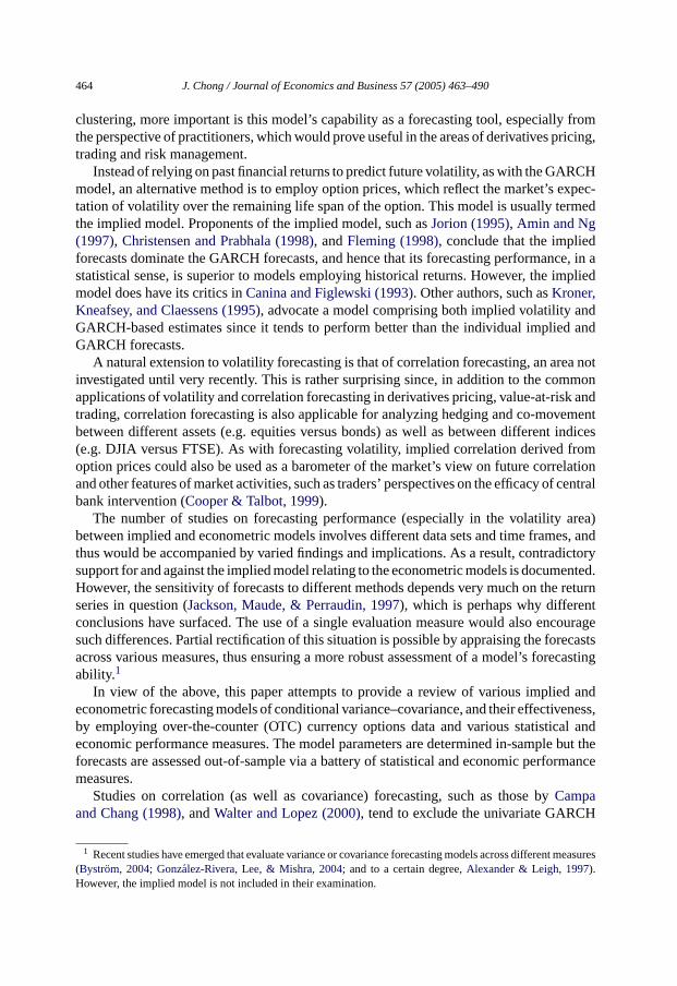
464 J. Chong / Journal of Economics and Business 57 (2005) 463–490

clustering, more important is this model’s capability as a forecasting tool, especially fromthe perspective of practitioners, which would prove useful in the areas of derivatives pricing,trading and risk management.

Instead of relying on past financial returns to predict future volatility, as with the GARCHmodel, an alternative method is to employ option prices, which reflect the market’s expec-tation of volatility over the remaining life span of the option. This model is usually termedthe implied model. Proponents of the implied model, such asJorion (1995), Amin and Ng(1997), Christensen and Prabhala (1998), andFleming (1998), conclude that the impliedforecasts dominate the GARCH forecasts, and hence that its forecasting performance, in astatistical sense, is superior to models employing historical returns. However, the impliedmodel does have its critics inCanina and Figlewski (1993). Other authors, such asKroner,Kneafsey, and Claessens (1995), advocate a model comprising both implied volatility andGARCH-based estimates since it tends to perform better than the individual implied andGARCH forecasts.

A natural extension to volatility forecasting is that of correlation forecasting, an area notinvestigated until very recently. This is rather surprising since, in addition to the commonapplications of volatility and correlation forecasting in derivatives pricing, value-at-risk andtrading, correlation forecasting is also applicable for analyzing hedging and co-movementbetween different assets (e.g. equities versus bonds) as well as between different indices(e.g. DJIA versus FTSE). As with forecasting volatility, implied correlation derived fromoption prices could also be used as a barometer of the market’s view on future correlationand other features of market activities, such as traders’ perspectives on the efficacy of centralbank intervention (Cooper & Talbot, 1999).

The number of studies on forecasting performance (especially in the volatility area)between implied and econometric models involves different data sets and time frames, andthus would be accompanied by varied findings and implications. As a result, contradictorysupport for and against the implied model relating to the econometric models is documented.However, the sensitivity of forecasts to different methods depends very much on the returnseries in question (Jackson, Maude, & Perraudin, 1997), which is perhaps why differentconclusions have surfaced. The use of a single evaluation measure would also encouragesuch differences. Partial rectification of this situation is possible by appraising the forecastsacross various measures, thus ensuring a more robust assessment of a model’s forecastingability.1

In view of the above, this paper attempts to provide a review of various implied andeconometric forecasting models of conditional variance–covariance, and their effectiveness,by employing over-the-counter (OTC) currency options data and various statistical andeconomic performance measures. The model parameters are determined in-sample but theforecasts are assessed out-of-sample via a battery of statistical and economic performancemeasures.

Studies on correlation (as well as covariance) forecasting, such as those byCampaand Chang (1998), andWalter and Lopez (2000), tend to exclude the univariate GARCH

1 Recent studies have emerged that evaluate variance or covariance forecasting models across different measures(Bystrom, 2004; Gonzalez-Rivera, Lee, & Mishra, 2004; and to a certain degree,Alexander & Leigh, 1997).However, the implied model is not included in their examination.

J. Chong / Journal of Economics and Business 57 (2005) 463–490 465

models,2 focusing their efforts on the multivariate GARCH and models such as the simplehistorical or exponentially weighted moving average (EWMA). Due to the simplicity ofthe univariate GARCH models relative to their multivariate counterparts, and their effec-tiveness at forecasting in the volatility area, these models are often used by academics andpractitioners alike. As such, so long as the conditional correlations predicted by the mod-els are within the bounds of (−1, 1), the univariate GARCH models should be includedfor analysis, and we have chosen to include four of the most prevalent types of univariateGARCH model.3

With the knowledge that the crucial objective in measuring forecast accuracy is the lossfunction, it is inevitable that the rankings of forecast accuracy may be very different acrossdifferent loss functions and/or different horizons (Diebold & Lopez, 1996). Thus far, theperformance criterion, or loss function, of choice in most studies on correlation (as well asvolatility) forecasting is the root mean squared forecast error (RMSFE). Widely upheld forits statistical objectivity, it may nevertheless be of little economic value from the viewpointof a practitioner. With this in mind, we are interested in determining whether a forecast thatperforms well under a statistical measure would do likewise under an economic criterion.Hence, over and above employing the RMSFE in ranking the performances of the variousforecasts, we also implement performance measures adopted by practitioners in the formof a reduction in the hedged portfolio’s volatility, value-at-risk (VaR) and trading profits.This would ensure that no one measure is used as the overriding criterion in determining amodel’s effectiveness in forecasting.

We show that econometric models outperform the implied model on the basis of both sta-tistical and financial measures. Despite the promise of the implied model in the volatility andcorrelation areas (as presented by proponents of the implied model), it has not been totallyeffective in predicting hedge ratios or in estimating VaR. On the other hand, the EWMAmodel produces hedged portfolios with the lowest variances, as well as VaR that cater tonegative portfolio returns. On trading profitability, the directional bets taken by the expo-nential GARCH (EGARCH) and GJR (acronym for the authors of this model—Glosten,Jaganathan, and Runkle) models in a simple trading strategy, on the whole, appear success-ful, reaping positive returns. Overall, it would appear that the EWMA model is the bestvariance–covariance forecasting model, at least with regard to the performance measuresexamined. This finding corroborates previous studies that show a simple model like EWMAperforms equally well against more sophisticated forecasting models.

The remainder of this paper is organized as follows. Section2 describes the data, fol-lowed by a discussion of the day-count convention in Section3. The methodologies of

2 For a multivariate forecasting model, one would only need two return series, in order to ascertain their condi-tional correlation. However, for a univariate forecasting model, a third return series is required. For example, if theconditional correlation between the returns of USD/DEM and USD/JPY is of interest, then the conditional GARCHvariances of the returns of USD/DEM and USD/JPY, as well as the returns of the cross-currency DEM/JPY, arerequired. This is evident in Eq.(A.11).

3 There are three incidences of conditional correlations exceeding the bounds of (−1, 1), and all are attributableto the GARCH-t model, for the USD/GBP, USD/DEM pair, at the daily, one- and three-month horizons. Eachexceedence is but 0.2% of the 534 out-of-sample observations. Further, as their magnitudes of exceedence aresmall (0.0559, 0.0002, and 0.0468, respectively), the conditional correlations were left unadjusted.


the forecasting models and evaluation measures are presented in Section4. Results arediscussed in the fifth section, while Section6 concludes.

2. Data

The data for the implied correlation and return series are from the options and spotrates of USD/DEM, USD/JPY, DEM/JPY, GBP/USD and GBP/DEM, for one- and three-month horizons. The data, provided by J.P. Morgan Chase, spans the period July 19,1993 to September 13, 1999 (1605 observations), and are collected daily at the same time(16:00 GMT) so as to avoid non-synchronous prices. A drawback of working with asyn-chronous data is that the value of a portfolio is never known at a point in time. Coupledwith the possibility of correlations being understated (Burns, Engle, & Mezrich, 1998),this would introduce systematic errors into the estimation of VaR, hedge ratios and assetallocations.

OTC currency options are used in this study, as opposed to the exchange-traded currencyoptions data (e.g. those listed on the Philadelphia Stock Exchange, PHLX) employed inmuch of the existing literature, for several reasons. First, the OTC currency options market ismore liquid; second, the time-to-expiration of OTC currency options is constant, mitigatingany possible effects from the varying times-to-expiration of exchange traded options; andthird, OTC currency options are quoted at-the-money forward, which reduces the ‘smile’effects when implied volatility varies with exercise price.

3. Day-count convention

We employ the modified day-count convention adopted by the industry in computing thevarious forecasts. Consider, for example, a one-month currency option. FollowingBreuerand Wohar (1996), the contract will settle in one calendar month from the spot value date,which is two business days from the spot transaction. If the day in which the contract settlesfall on a non-business day, the settlement date is moved forward to the next business day.However, if the next business day crosses into the next calendar month, then the settlementdate is moved backward to the previous business day. As such, the time-to-expiration forthe one-month currency option in our sample ranges from 23 to 27 trading days, whilethat of the three-month currency option ranges from 66 to 69 trading days. For comparisonacross forecasts, historical models (such as GARCH, etc.) would also have to adhere to theday-count convention.

4. Methodology

4.1. Forecasting volatility/correlation

In this study, we employ 10 forecasting models: The simple historical, EWMA, GARCH,EGARCH, GJR, GARCH-t, VECH (a column stacking operator), BEKK (acronym for


the original authors of this model—Baba, Engle, Kraft, and Kroner), dynamic conditionalcorrelation (DCC), and implied.Appendix Aprovides a detailed description of the models.

4.1.1. Deriving daily results for the implied modelFor comparison across the different performance measures, daily results must be avail-

able. However, this is not possible as the implied data are for monthly horizons only. Thereare basically three approaches to estimating the daily quotes:

1. Extrapolation: Taking the gradient between one- and three-month implied volatilities,and assuming the same between the one-day and one-month implied volatilities to derivethe one-day figure.

2. One-month estimationmethod: Assuming one-day implied volatility with the one-monthimplied volatility, as inLopez and Walter (2001). The one-day forecasts are generated byassuming constant volatility, i.e. by employing the square root of time rule for standarddeviations. An obvious shortcoming of this method is the mismatch between the one-dayimplied volatility and the one-day benchmark. Errors in forecasting, already inherent insuch an assumption, will be further compounded by using a mismatched benchmark.

3. Term structure of implied volatilities: Employing the concept of implied volatility termstructure, which refers to the relationship between implied volatilities of options withdifferent maturities. We adopt the method byHeynen, Kemna, and Vorst (1994), involv-ing the testing of volatility models based on the closeness of the forecast volatility and theimplied volatility term structures.4 The relation between average variances with differingtimes-to-maturity is represented by

(ht,T1 − h) = T2

T1

(α+ β)T1 − 1

(α+ β)T2 − 1(ht,T2 − h) (1)

whereh = γ/(1 − α− β), γ, α, β as in Eq.(A.6), andT1 >T2. The one-day (T2) impliedvolatility is then determined from either the one- or three-month (T1) implied volatility.For example, to derive the one-day implied volatility from a one-month implied volatility,T2 = 1 andT1 is the number of trading days in a month using the day-count conventionabove.ht,T1 = σ2

t,T1is the implied variance for the one-month option. Rearranging(1), we

have the one-day implied variance

ht,T2 = T1

T2

(α+ β)T2 − 1

(α+ β)T1 − 1(σ2t,T1

− h) + h,

from which to compute the one-day implied volatility.

4.1.2. Multiple day forecastsTo estimate the parameters of the various GARCH models, the first 1000 data points

are used as in-sample data (July 19, 2003 to May 20, 1997), with the out-of-sample period

4 The term structure described in(1) is employed for GARCH models. For it to be applicable to implied variances,there must be a close correspondence between the mean annualized GARCH variance and mean annualized impliedvariance. This is the case since the difference between the two variances for the various currencies is less than 1 %(not shown, but available from the author on request).


running from May 21, 1997 to June 8, 1999 (534 data points). In the case of univariateGARCH models, each of the three currency return variances is separately estimated as aunivariate process, and their covariances are derived via(A.11).5 For multivariate GARCHmodels, covariances and variances are jointly determined. Taking the GARCH(1,1) modelas an example, once its parameters have been estimated during the in-sample period, futurevalues of the conditional variance can be forecast recursively with

ht+n = γ + (α+ β)ht+n−1 (2)

where hτ denotes the daily estimate of the conditional variance for dayτ. γ, α, and βrepresent the estimates for parametersγ, α, β, andβ, respectively. This formula is onlyoptimal forn≥ 2. Forn= 1, we useht+1 = γ + αε2

t + βht . Since variances are additive intime,

∑Tn=1ht+n would be the variance forecast at timet over the nextT days.6 The same

logic applies to the covariance forecast.While most GARCH models provide an easy method to generaten-step ahead forecasts

(as in (2) above), it is not so with the DCC evolution process, which is non-linear. Then-step covariance forecast is represented by

Qt+n = (1 − α− β)Q+ α(Ξt+n−1Ξ′t+n−1) + βQt+n−1,

where Et(Ξt+n−1Ξ′t+n−1) = Et(Rt+n−1) and then-step correlation forecast,Rt+n =

Q∗−1t+nQt+nQ∗−1

t+n . We therefore follow the suggestion byEngle and Sheppard (2001), wherethe unconditional covariance approximates the unconditional correlation, i.e.Q ≈ R andEt(Qt+1) ≈ Et(Rt+1). Hence, this forecast uses the method that directly solves forwardRtvia

Et(Rt+n) =n−2∑i=0

(1 − α− β)R(α+ β)i + (α+ β)n−1Rt+1.

Using each model, multi-step ahead forecasts are constructed for up to three months (69days) following the 1000-day in-sample estimation period. The sample is then rolled for-ward, the parameters re-estimated using observations 2–1001, and forecasts again computedup to three months hence. This procedure is repeated until the full sample is exhausted.

To obtain a starting value for the computation of the EWMA model, the 1000 in-sampledata points are used to calculate the initial variance, which is set as the statistical varianceof those 1000 data points. Eqs.(A.3) and (A.4)are then imposed to obtain the variance andcovariance, respectively, until the end of the in-sample period and subsequently to forecastconditional covariances and variances for the out-of-sample period. For the simple historicalmodel, the 1000 in-sample data points are used for variance and covariance computation,

5 Following the example in footnote 2, we shall input the conditional GARCH variances of the returns ofUSD/DEM (h(x)t), USD/JPY (h(y)t), and DEM/JPY (h(x− y)t) into (A11). Forecasting conditional correlationvia univariate GARCH models is different from the constant conditional correlation model ofBollerslev (1990)since the GARCH conditional correlation is time varying.

6 While the logarithmic specification of the EGARCH ensures that volatility is always positive, the futureexpected variance beyond one period cannot be computed analytically. To calculate the variance over the nextT days, we transform lnht of Eq. (A.7) to ht = e(γ+β ln ht−1+αzt−1+ϕ(|zt−1|−

√2/π)), compute the daily variances

recursively, and then summing them up to obtain the total variance.


which are then taken to be the one-day forecast. In these cases, since the variance andcovariance are additive, the one-day forecast is simply multiplied byT days to obtain theTperiod variance and covariance, respectively.

4.2. Evaluation criteria

We shall employ four evaluation criteria: statistical, the reduction of hedged portfoliovolatility, value-at-risk, and trading profits. The forecasts are essentially evaluated on a dailybasis and then averaged over the out-of-sample period to arrive at the rank of the model.

4.2.1. StatisticalThe statistical evaluation measure, most commonly employed in academic research, is

the root mean squared forecast error (RMSFE).7 It is represented by

et = ρ(x, y)t − ρ(x, y)t (3)

RMSFEt =√√√√ T∑

t=1

(et)2

T(4)

whereρ(x, y)t andρ(x,y)t are, respectively, the forecast and realized (or implied) correla-tions ofX andY returns at timet. While it is common to determine the RMSFE against arealized value, a different ex post measure worth considering, thus far not common in thecurrent literature, is that of the implied variable. Comparing different forecasts with such ameasure has the benefit of assessing how good a proxy the various forecasts are to marketviews.

To compare the predictive accuracy of alternative forecasts, we employ an asymptotic testof the null hypothesis of no difference in the accuracy of two competing forecasts (Diebold& Mariano, 1995). Given any loss function, in this case a squared error loss function, wegenerate a time series of the differences between the loss function values of each forecastand the best forecast. A mean of zero for this difference implies that the two forecasts areequally accurate. However, should we reject the null hypothesis, then the forecast with thelower squared error is the more accurate forecast.

4.2.2. Reduction of hedged portfolio volatilityThe objective of a hedge is to reduce the risk of investing in a currencyX (for example,

USD/DEM) by holding an offsetting position in another currencyY(for example, USD/JPY)or in a currency futures contract (a USD/DEM futures). To gauge the effectiveness of ahedge, we evaluate the variability of the investor’s portfolio8 and the hedge that results

7 There is a wide variety of statistical evaluation criteria, such as the mean forecast error, mean absolute error,mean absolute percentage error, relative absolute error, etc. We employ the RMSFE due to its popularity amongpractitioners and academics (Carbone & Armstrong, 1982), and that it is the most appropriate measure for selectinga forecast model (Makridakis & Hibon, 1995).

8 The portfolio comprises of the currency in which the investor is exposed to (e.g. USD/DEM), and the currencyused for hedging (e.g. USD/JPY). As a result, the daily portfolio return isxt +βtyt, where at timet, xt andyt arethe returns for USD/DEM and USD/JPY, respectively, andβt is the optimal hedge ratio.


in the largest out-of-sample volatility reduction for the hedged portfolio, as compared tothe no-hedge outcome, is considered the most effective (Kroner & Sultan, 1993). To thisend, at every time step, the optimal hedge ratio (OHR), the hedge ratio that minimizes theconditional variance of the hedged portfolio, has to be computed and is presented as

βt = −h(x, y)th(y)t

. (5)

A detailed description of the OHR can be found inKroner and Sultan (1993).

4.2.3. Value-at-risk (VaR)VaR is defined as a measure of the maximum potential change expected in the value of a

portfolio with a given probability over a pre-determined horizon (Morgan, 1996). It is also aregulatory disclosure requirement by theBasle Committee on Banking Supervision (1996,1998) for capital adequacy and in financial reports. A further motivation for employingVaR as an evaluation tool is the many recent studies on forecast evaluation that have used itexclusively as the financial measure of choice (Brooks & Persand, 2003; Engle & Sheppard,2001, among others). In this study, we shall focus on two ways of computing the VaR ofa portfolio – the variance–covariance approach (VCV) and portfolio aggregation (PA) –using the 95% and 99% confidence levels, with forecast horizon of one-day.

The ingredients for the VCV computation are the return volatilities (variances) of theindividual assets that form the portfolio, and the correlation (covariance) between the returns.This has the advantage of allowing users to assess directly the effects that volatilities andcorrelations have on their VaR estimates. Assuming that the portfolio consists of two assets,the portfolio conditional variance is calculated via

hp = a2h(x) + b2h(y) + 2abρ(x, y)√h(x)

√h(y), (6)

whereh(x) andh(y) are the conditional variances of the returns ofX andY, respectively,ρ(x,y) is the conditional correlation between the returns series, witha andb being theproportion invested in the respective assets (in this study,a=b= 0.5). Using the notation ofBrooks and Persand (2003), the VaR is calculated as

VaRip,t(N,α) = [Fit,N ]

−1( α

100

)√hip,t,N, (7)

where VaRip,t(N,α) is the portfolio VaR at timet, determined by modeli (being any of the

10 models previously described),N is the forecast horizon, [Fit,N ]

−1is the inverse of the

cumulative distribution function,α is the percentage significance level and√hip,t,N is the

square root of the portfolio conditional variance determined by modeli. The cumulativedistribution function commonly employed in risk management literature is that of the normaldistribution, while the percentage significance level is either 1% (in line with the BasleCommittee’s recommendation) or 5% (commonly used by banks for their internal riskreporting).

The approach based on the PA principle was first proposed (Zangari, 1997) as a flexibleand efficient alternative to VCV. It alleviates the difficulty with estimating large volatility andcorrelation matrices as encountered by VCV, and instead simply estimates the volatility of


the portfolio returns. Univariate models are also much simpler and tractable than multivariatemodels. Assuming that the portfolio returns are distributed according to the conditionalnormal distribution, as undertaken by VCV, VaR is as(7), with the portfolio variancemodeled the same way as the individual component assets. There is no necessity for theestimation of individual volatilities and correlations between the various time series.

We evaluate the VaR models by examining their percentage of exceedences in a hold-out sample. Any model that has a percentage of exceedences in the out-of-sample periodgreater than that specified by the VaR model is rejected as inadequate and hence would havethe worst rank. For cases where the percentage of exceedences is lower than the nominalvalue, a model whose failure rate is closer to the nominal number is considered better (andhence would rank higher) than its comparatively conservative counterpart. We thus arguethat an asymmetric loss function should be used in evaluating the VaR models, with toomany exceedences, that is, days where the VaR is insufficient to cover the actual portfoliolosses, deemed more serious than situations where the model has generated excess capital.9

4.2.4. Trading profitsAnother criterion that could be employed to appraise forecast effectiveness is by investi-

gating the profitability of trading strategies formed from the forecasts (Noh, Engle, & Kane,1994). While the other measures are related to risk, this is the only criterion that considersthe profitability associated with forecasting.Noh et al. (1994)investigate profitability fromvolatility trading, whereasGibson and Boyer (1998), andBystrom (2002)examine fore-cast success from correlation trading. However, the data used in the studies on correlationtrading are simulated. Instead, we employ actual market quoted instruments.

Assuming that an investment of DEM 100 worth of straddles are bought and sold, withoutreinvestment of profits, then on each day, each agent applies a forecasting algorithm inestimating the volatility of tomorrow and hence effectively also forecasting the straddleprice of tomorrow. If the straddle price forecast is greater (less) than the closing straddlemarket price for today, then the straddle is bought (sold). Thus, the rate of return on buyingand selling straddles will be

rit+1 = rt+1(hit+1) =

100

VM,t(VM,t+1 − VM,t) if bought straddle

− 100

VM,t(VM,t+1 − VM,t) + 200rdt+1 if sold straddle

, (8)

whereVM,t andVM,t+1 are, respectively, the market prices of the straddle at timet andt+ 1,hit+1 the conditional variance forecast of modeli for t+ 1, rdt+1 the domestic interest rateat time t+ 1 (where the proceeds of DEM 100 and the initial DEM 100 are invested in arisk free asset when a straddle is sold). A filtering strategy is also undertaken so that tradesoccur only when the straddle price is expected to change in excess of 2 and 5%.

The pricing model for currency options commonly employed is theGarman–Kohlhagenmodel (1983), in which we replace the constant variance variable with the conditional vari-

9 An alternative would be to compare the number of exceedences to the nominal value and deem the methodwith the smallest deviation from the theoretical value the best method. Overall, there is only a slight change inrankings among the forecasts (the results are available from the author upon request).


ance forecast of modeli,hit+1|t . Since an at-the-money forward straddle is just a combination

of an at-the-money call option and an at-the-money put option,V it+1|t = Cit+1|t + Pit+1|t ,

whereCit+1|t andPit+1|t are the Garman–Kohlhagen call and put currency option priceforecasts of modeli for t+ 1 att. With the modified Garman–Kohlhagen, the variance fore-casting abilities of the various models are under review since the variable of interest ishit+1|t . To evaluate the models’ correlation forecasts,hit+1|t would have to be replaced by

hit+1|t , represented as

hit+1|t (x− y) = σ2t+1 (x) + σ2

t+1 (y) − 2σt+1 (x) σt+1 (y) ρit+1|t (x, y) (9)

whereσ2t+1(x) andσ2

t+1(y) are the implied variances of theXandY returns,xandy, respec-tively, at timet+ 1, andρit+1|t(x, y) is the correlation forecast betweenx andy predicted bymodel i for t+ 1 at t. So if the straddle of the cross currency (represented by the variablex− y) JPY/DEM is to be priced, isolating the effects of the correlation forecast, thet+ 1implied volatility quotes for DEM/USD and JPY/USD straddles as well as the correlationforecast between the returns of DEM/USD and JPY/USD are utilized.

5. Results

Please refer to the results, presented inTable 1, Panels A and B for the currency pairs ofUSD/DEM, USD/JPY and USD/GBP, USD/DEM, respectively.

5.1. Statistical

The common currencies involved in our study and those cited byCampa and Chang(1998)andWalter and Lopez (2000)are USD/DEM and USD/JPY. For both one- and three-month horizons,Campa and Chang (1998)find the implied correlation forecast to have thesmallest RMSFE whileWalter and Lopez (2000)have the VECH as the best correlationforecasting model. In our study, the EWMA model performs best for both forecastinghorizons, with its forecasts statistically different from that of the other models (Table 2).The differences in conclusion10 between the three studies should not be delved into toodeeply as they are probably due to different in- and out-of-sample horizon lengths, and thedifferent times at which the data are collected. The in-sample data are approximately thesame for the three studies, employing about four years worth of observations. The out-of-sample forecasts are approximately 6.5 years forCampa and Chang (1998), 6.5 years forWalter and Lopez (2000), and two years for this study. It is not indicated inCampa andChang (1998)or Walter and Lopez (2000)if their currency and currency options data arecollected at the same time. This could result in errors caused by non-synchronous prices.As mentioned previously, our currency and option data are collected at 16:00 GMT.

10 Jackson et al. (1997)deduce that the forecastibility of variables (be it volatility or correlation) and the sensitivityof forecasts from different methods depend very much on the return series in question whileDiebold and Lopez(1996)conclude that rankings of forecast accuracy may be very different across different loss functions and/ordifferent horizons.

J.Chong/Jo

urnalofEconomics

andBusiness57(2005)463–490

473

Table 1Average rank performance of forecasting models across measures, currencies, and horizons


Tabl

e1

(Continued)

476J.C

hong/Jo

urnalofEconomics


Table 1 (Continued)

Note: The average overall rank for the implied model (including the daily estimates) is 6.33.

J.Chong/Jo

urnalofEconomics


477

Table 2Diebold and Mariano (1995)test of accuracy for correlation forecasts under the root mean squared loss function

Benchmark currencieshorizon

Realized correlation Implied correlation

USD/DEM, USD/JPY USD/GBP, USD/DEM USD/DEM, USD/JPY USD/GBP, USD/DEM

One-month Three-month One-month Three-month One-month Three-month One-month Three-month

Forecasting modelsVECH 5.42** 9.05** 6.86** 8.79** – 1.29 4.93** –BEKK 9.59** 13.87** 7.84** 9.13** 5.35** 4.17** 7.20** 2.72**

GARCH 2.36* 6.87** 7.68** 8.99** 11.96** 10.94** 3.81** 1.32EGARCH 6.97** 9.44** 6.68** 7.81** 11.84** 9.69** 4.89** 3.88**

GJR 6.90** 8.98** 6.67** 7.20** 11.14** 7.64** 3.93** 1.21GARCH-t 6.90** 9.73** 3.35** 2.88** 14.53** 12.98** 3.00** 0.74Implied 11.29** 15.45** 8.40** 11.57** N.A. N.A. N.A. N.A.EWMA – – – – 8.85** 12.39** 3.99** 3.11**

Simple historical 15.06** 24.48** 6.62** 8.97** 18.17** 23.15** 7.00** 1.62DCC 12.17** 14.84** 11.64** 16.59** 2.82** – – 3.20**

* Indicates statistical significance at the 5% level.** Indicates statistical significance at the 1% level.


The performance of the implied model in both one- and three-month USD/DEM,USD/JPY correlation forecast is dismal. It ranks seventh in terms of RMSFE. This said, itshould be noted that implied correlations (or volatilities) should be viewed differently fromstatistical correlations (volatilities). Implied correlations are correlation forecasts that areimplicit in option prices, with the forecast horizon equivalent to the maturity of the option.The implied model employs current option prices; hence it embodies all of the investors’expectations about the likely evolution of the underlying asset. On the other hand, statisti-cal models employ the historical prices of the underlying asset. In contrast, the models thatconsistently achieve the smallest RMSFE for both the one- and three-month periods are theVECH, GARCH, GJR, and EWMA models.

On the USD/GBP, USD/DEM pair, the EWMA model once again has the lowest correla-tion RMSFE (at both the one- and three-month horizon), and it is statistically different fromthe other forecasts. The other models that perform well overall are the GARCH-t, GJR, andGARCH. In comparison to its previous performance, the VECH model did poorly, comingin ninth in both the one- and three-month correlation forecasts. Excluding the univariateGARCH models from the comparison – for consistency with the studies byCampa andChang (1998)andWalter and Lopez (2000)– the implied model has a lower RMSFE thanthe VECH model for both one- and three-month. However, it still does poorly relative tothe EWMA model.

In contrast to its dominant performance across currency pairs with the realized correlationas benchmark, the EWMA forecast, when assessed against the implied correlation, is goodonly at the one-month horizon. The VECH and DCC models, in this instance, produce fore-casts that are closest to market predictions in terms of RMSFE across different currency pairsand horizons while the GJR and GARCH-tmodels, consistent in their forecasts of USD/GBP,USD/DEM correlation, is accompanied by the BEKK for its reliability in the forecast ofUSD/DEM, USD/JPY correlation. Nevertheless, it should be noted that the VECH per-formance for the USD/GBP, USD/DEM correlation, at the three-month horizon, is notstatistically different from those of GARCH-t, GJR, simple historical, and GARCH models.

5.2. Reduction of hedged portfolio volatility

For the out-of-sample hedge ratio forecasts concerning the USD/DEM, USD/JPY pairover the daily horizon, the implied models are very impressive, dominating the top threepositions and registering the largest reductions in volatility of the hedged portfolio overthe no-hedge position. On the longer dated horizons, the EWMA is by far the best model.It ranks first in three cases and is runner-up on one occasion. Two possible grounds forthe accurate predictions of a relatively simple model like the EWMA: (1) it is better ableto generalize and has not been over-fitted to features of the data that are specific to thein-sample estimation period, and (2) it does a better job at capturing the unconditionalmoments that the longer horizons revert to.

Overall with the longer horizons, the VECH is the next best model, followed by theunivariate GARCH model. At the other end of the spectrum, the simple historical modelis the worst performer. Modified GARCH models that capture additional stylized featuresof the data, such as the GARCH-t (fat tails), or the GJR (asymmetries) models performreasonably, although they are not the best models. In particular, these results suggest that


there seems little benefit in attempting to capture asymmetries in volatility if the objectiveis to hedge currency risk.

Regarding the daily hedge ratio forecasts with USD/GBP and USD/DEM, once again theimplied models are dominant. For the one- and three-month horizons, the GARCH-tmodelappears best, followed by the EWMA model. The rest of the models are not as consistentin their performances. The VECH and the simple historical models did reasonably well forthe three-month horizon but less so for the shorter period of one-month. The EGARCH andimplied models also perform poorly over one-month.

Overall, for the longer dated horizons, the implied model has been a disappointment withregard to the forecast of the OHR. Existing literature has shown the implied volatility derivedfrom the options market to be effective in forecasting realized volatility and correlation,though there has also been evidence to the contrary (Canina & Figlewski, 1993). It wouldappear that the effectiveness of the implied model is dependent on the criterion used. Themajority of the studies that argue for the superiority of the implied model over time seriesmodels employ the RMSFE criterion to evaluate the forecasts. It is certainly not necessarilythe case, as is observed here, that the same models are preferred in the context of hedgingeffectiveness.

Our results do not contradict those ofSiegel (1997)– who finds that the implied betahedge ratio performs better than the regression-based beta hedge ratio – since we also findthat variance and covariance forecasts derived from traded options yield “better” hedgeratios than those based on ordinary least squares estimation. We do find, however, othertime series models that are superior to both.

5.3. VaR

5.3.1. USD/DEM, USD/JPYWith regard long USD/DEM, USD/JPY using the variance–covariance approach (VCV),

the BEKK model is best at the 99% level of confidence, followed jointly by the implied(extrapolation) and the implied (one-month) models.11 For the short USD/DEM, USD/JPYportfolio returns at the 99% confidence level, the GJR and EWMA models are tied forfirst, accompanied by the VECH and EGARCH models. As with the long portfolio at the95% level, GARCH once again emerges at the top. Applying the portfolio aggregation (PA)approach to long portfolio returns, the EGARCH model is best, followed by the GARCHmodel. The case of short portfolio returns is where we observe the effectiveness of thesimple historical and EWMA models emerging. Under the VCV approach and now withPA, EWMA is equal first at the 99% confidence level, accompanied by the GARCH andGJR models. The simple historical model, coming in second at the 95% level with VCV, isnow ranked best (with GJR) under PA.

11 Note that the option maturities of our data set are longer than the one-step ahead forecasts in our analysis.However, since the option pricing model assumes constant second moments over the life of the option (taking theone-month horizon), one-day forecasts could be generated by assuming that daily innovations are independent anddividing the implied variances by the number of days in a month (taking into account the day-count convention).This is also the approach taken byLopez and Walter (2001). Although we have introduced three ways of computingone-day implied forecasts, implied (one-month) is the only approach that employs market quoted options.


5.3.2. USD/GBP, USD/DEMUnder the VCV approach for long portfolio returns, implied (one-month) is the preferred

model at the 99% confidence level, followed by the implied (extrapolation) model. At the95% level of confidence, the GJR model tied for first with the BEKK, EGARCH and DCCmodels. In the short portfolio case, seven models ranked equal first at the 99% level. As withthe short USD/DEM, USD/JPY portfolio, the simple historical and the EWMA models arebeginning to show their prominence with consistent performances on short portfolio returns.Now we turn our attention to PA where the simple historical and EWMA models, once again,excel in the estimation of short portfolio VaR, with both models capturing the top position atthe 99% confidence level, and the EWMA model joint first at the 95% level. The outstandingperformance of these two models in estimating VaR for the short portfolio returns partiallyvalidates the specifications of the simple average forecasts and provides support for thecommon industry practice of using these models (Lopez and Walter, 2001).

At this moment, it is appropriate to introduce differentiating forecasts of the same rank,with the aid of the mean VaR,VaR = (1/T )

∑Tt=1VaRt and the standard deviation of VaR,

S.D. (VaR) =√

(1/T − 1)∑T

t=1(VaRt − VaR)2. It is intuitive for models with higher mean

VaR estimates to have lower percentages of exceedences as a higher VaR would have a betterchance of preventing an exceedence of returns over the threshold. However, we should alsoconsider the standard deviation of the VaR estimates. A higher standard deviation togetherwith a lower VaR mean suggest that in the context of VaR modeling, a model is better atforecasting the fluctuation of portfolio returns and hence has the ability to respond to everchanging market conditions. Another case is that of a forecast with a lower mean VaR, lowerVaR standard deviation and lower percentage exceedences. A possible implication is thatthe model is better at timing the peaks and troughs of portfolio returns than an alternativemodel.

In a separate study (available from the author on request), it is noted that for the longportfolio, VaR estimates tend to exceed the 1% failure threshold (at the 99% confidencelevel) but this is not the case for the short portfolio. However, at the 95% confidence level(commonly used by banks for their internal risk management purposes), the majority ofmodels did not violate the 5% tolerance level. Thus, the 99% coverage rate presents a muchmore severe test of the forecasting ability of the models. However, to increase the power ofthe test, the 95% coverage rate should be employed since one would be able to observe asufficient number of deviations to validate the model. We also discover that the differencesin mean and standard deviation of the models’ VaR for both approaches are slight, withlower average estimates for PA. This, however, has not translated into an obvious distinctionwhen scrutinized from the angle of percentage exceedences. It augurs well for PA, which,despite its relative computational ease, adheres as well to its statistical specification as VCV,and hence could be considered just as reliable.

5.4. Trading profits

5.4.1. Profits from volatility tradingFirst, an examination of the profits generated by the volatility forecasting models for OTC

JPY/DEM and GBP/DEM straddles is conducted, the results of which could be compared


Fig. 1. Trading profits from DEM/JPY volatility forecast.

to similar studies (though of different instruments) byHarvey and Whaley (1992)andNohet al. (1994).

With JPY/DEM straddles at all three filters, EWMA is best at predicting the directionalchange of volatility. The performance of EWMA is followed by GARCH-t and EGARCH.The main cause for the models’ dismal performances (as illustrated inFig. 1) is their inabilityin predicting the volatility change of October 7, 1998 and October 8, 1998 amidst the Asiancrisis, where a wrong prediction would reduce profits by 38.60% and 66.63%, respectively.A reason in part for EWMA’s exceptional performance is its successful forecast of such achange on October 7, 1998. Prior to those two fateful days, the models performed well andregistered healthy returns. This result confirms previous findings that, with no transactioncosts, GARCH models do have predictive power and hence could be employed as tools forprofitable trading strategies.

With regard the rate of return for GBP/DEM straddles trading, the most dependablemodel is the GJR, coming in within the top three positions for each of the filter levels. Thisis a sharp distinction from its performance with JPY/DEM straddles trading. GARCH rankssecond under no filter and 2% filter. However, its form dips in the 5% filter, reflecting thelack of profitable opportunities with smaller price swings as a result of imposing a higherfilter. A surprise would have to be the outstanding accomplishment achieved by the simplehistorical model under a 5% filter. Its top rank goes to show that in spite of its simplicityrelative to its more sophisticated peers, its computational ease could be advantageous forprofitable trading under less volatile scenarios. This time round, EWMA performs poorly,with fellow laggards in the VECH and BEKK models.

5.4.2. Profits from correlation tradingThe following section, executed in the spirit ofGibson and Boyer (1998), will describe

briefly the models’ correlation forecasting capability, applying the forecast of USD/DEM,USD/JPY correlation for JPY/DEM straddles trading and that of USD/GBP, USD/DEMcorrelation for GBP/DEM straddles.


Trading DEM/JPY straddles with USD/DEM, USD/JPY correlation forecasts for filtersof less than 2%, GJR and BEKK are the two best models, while at the 5% filter, GARCH-tand VECH inherited that title. This suggests that the strength of GJR and BEKK lie withdirectional bets on straddle prices of less than 2% while the forte of GARCH-t and VECHare with price swings of larger than 5%.

In the trading of GBP/DEM straddles, this time with just the USD/GBP, USD/DEMcorrelation forecasts, EGARCH lead for all filter levels, followed by GJR. The success ofthe models is attributed to the stability of the GBP/DEM returns volatility, in contrast to thevolatility of the JPY/DEM returns.

6. Conclusion

The primary objective of this paper has been to assess the forecasting abilities of impliedand econometric forecasting models under statistical and financial evaluation measures,which has the advantage of not relying on any one criterion for forecast evaluation, ensur-ing robustness in the conclusions—this is akin to investing in a portfolio of stocks, wherebyone does not run the risk of relying on any one criterion. To this end, the study hassought to provide a review of various models available for the prediction of conditionalvariance–covariance, and their effectiveness. Ten models are introduced for comparison:the simple historical, EWMA, GARCH, EGARCH, GJR, GARCH-t, VECH, BEKK, DCCand implied.

Highly regarded for their objectivity, their utility for financial modeling and forecastevaluation, statistical criteria such as the RMSFE have long been considered the de factomeasure, among academics, in evaluating forecasting performances. The enthusiasm ofacademics for statistical evaluation, however, may not match the interests of practitioners,who would naturally view financial performance measures as more pertinent. In our attemptto address this discrepancy, we examine the performances of forecasting models acrossfinancial criteria such as volatility reduction of a hedged portfolio, value-at-risk and tradingprofits. This approach also has the advantage of not relying on any one measure for forecastevaluation, ensuring robustness in the results.

From the findings, it would appear that econometric models outperform the impliedmodel on the basis of both statistical and financial measures. Despite the promise theimplied model holds in the volatility and correlation arena, it has not been totally effectivein predicting hedge ratios. Further, the outcome presented by the VaR criterion also suggeststhat the implied model is not effective in estimating VaR. Hence, there is a possibilitythat market expectations as determined from the options market may not be as efficient inforecasting volatility for determining hedge ratios and/or VaR as they are for forecasting thevolatility and/or correlation themselves (as presented by proponents of the implied model).

On the other hand, the EWMA model – employing an exponential weighting schemefor variances and covariances – produces hedged portfolios with the lowest variances. Thedirectional bets taken by the model in a simple trading strategy, to a certain extent, appearsuccessful, reaping positive returns. This corroborates with studies that endorse a simplermodel like EWMA, in performing equally well against more sophisticated forecastingmodels with wealth accumulation. A possible rationale for the accurate predictions of a


relatively simple model like the EWMA is that it is better able to generalize and has notbeen over-fitted to features of the data that are specific to the in-sample estimation period.With the ease of constructing such models, it might not be worth the effort implementingmore complex and cumbersome models like the multivariate GARCH.

Overall (in Table 1), it would appear that the EWMA model is the bestvariance–covariance forecasting model, at least with regard the performance measuresexamined. Our study corroborates withAlexander and Leigh (1997), who also find EWMAto outperform GARCH. This confirms the faith that practitioners placed on the EWMAmodel for irrespective of the statistical or financial criterion, it has been consistent in itsprediction. Its appeal is further enhanced by its economical implementation, saving onhuman as well as computer resources. This said, a cautionary note byNelson (1992)is inorder. He argues that, at high frequencies, if the price generating process is a diffusion, thenthere is so much information with regard to conditional variances that even a misspecifiedmodel could be a consistent filter. On the other end of the performance spectrum is thesimple historical model. Its poor performance is expected since it does not account for thetime varying nature of covariances and variances, a phenomenon widely shown to exist inthe structure of financial returns. However, it is disappointing to note that, when tested witha battery of performance measures, the univariate and multivariate GARCH models do notquite measure up to the accolades of their advocates, considering their complexity in bothstructure and implementation.

Acknowledgements

I would like to thank Kenneth Kopecky, Ravi Shukla, two anonymous referees, PCVenkatesh, and participants at the Financial Management Association 2004 and CaliforniaState University, Northridge (CSUN) seminar series for their helpful comments and sugges-tions, which vastly improved a previous draft of this paper. A grant from CSUN in supportof this study is also gratefully acknowledged.

Appendix A. Description of forecasting models

A.1. Simple historical

The simple historical model simply estimates forecasts via the statistical (or uncondi-tional) variance and covariance. They are respectively represented by

h(x)t+1 = 1

n

n∑i=0

x2t−i, h(y)t+1 = 1

n

n∑i=0

y2t−i (A.1)

and

h(x, y)t+1 = 1

n

n∑i=0

xt−iyt−i (A.2)


wherex andy refer to the daily logarithmic returns for assetsX andY, respectively, whilext is x at timet.

A.2. EWMA

An exponentially weighted moving average (EWMA) places more weight on more recentobservations. Weights associated with previous observations decline exponentially overtime. In recognizing the dynamic nature of return variability, the EWMA has an advantageover the simple historical, which could lead to an abrupt change in volatility once the shockfalls out of the measurement sample. Further, if the shock is still included in a relativelylong measurement sample period, then an abnormally large observation will imply that theforecast will remain at an artificially high level even if the market is subsequently tranquil.The EWMA variance and covariance are respectively denoted by

h(x)t+1 = (1 − λ)∞∑i=0

λix2t−i, h(y)t+1 = (1 − λ)

∞∑i=0

λiy2t−i (A.3)

and

h(x, y)t+1 = (1 − λ)∞∑i=0

λixt−iyt−i. (A.4)

λ is assumed to be 0.94 (Morgan, 1996).

A.3. GARCH(1,1)

By far the most successful volatility forecasting model is the GARCH(1,1), developed byBollerslev (1986). It describes the volatility dynamics of almost any financial return series,across markets (e.g. emerging versus developed markets) and assets (e.g. stocks, bonds,commodities, indices, foreign exchange). The GARCH(1,1) variance,ht, is represented by

xt = µ+ εt, εt ∼ N(0, ht), (A.5)

ht = γ + αε2t−1 + βht−1 (A.6)

subject toγ > 0,α, β≥ 0, α+β < 1.α andβ coefficients determine the short run dynamicsof the resulting volatility time series. A largeβ indicates that shocks to conditional variancetake a long time to dissipate; that is, volatility is said to be “persistent.” A largeα indicatesthat volatility reacts intensely to market movements.

Although the GARCH model captures thick tailed returns and volatility clustering, phe-nomenon that are evident in financial returns, it is unable to account for any asymmetricresponse of volatility to positive and negative shocks since the conditional variance in(A.6)is a function of the magnitudes of the lagged residuals and not their signs. However, it hasbeen argued that a negative shock to financial time series is likely to cause volatility torise by more than a positive shock of the same magnitude. In the case of equity returns,such asymmetries are typically attributed to leverage effects or risk premium effects. In theformer theory, a fall in the value of a firm’s stock causes the firm’s debt to equity ratio to rise.


This leads shareholders, who bear the residual risk of the firm, to perceive their future cashflow stream as being relatively more risky. In the latter theory, news of increasing volatilityreduces the demand for a stock because of risk aversion. The subsequent decline in stockvalue is followed by increased volatility as forecast by the news.

Although asymmetries in currency returns cannot be attributed to the leverage or the riskpremium effects, there is equally no reason to suppose that such asymmetries do not exist.Studies have shown foreign exchange to exhibit volatility asymmetry (Aguirre & Saidi,2000; Balaban, 2004; Hu, Jiang, & Tsoukalas, 1997; Kim, 1998; McKenzie, 2002; Tse &Tsui, 1997; Tsui & Ho, 2004), with the hypothesis that the cause for such behavior is dueto central bank intervention (McKenzie, 2002).

Two popular asymmetric formulations are employed in this paper: the exponentialGARCH (EGARCH) model proposed byNelson (1991), and the GJR model, named afterthe authorsGlosten, Jaganathan, and Runkle, 1993.

A.4. EGARCH(1,1)

In the EGARCH(1,1) model, the natural logarithm of the conditional variance followsthe process below:

ln ht = γ + β ln ht−1 + αzt−1 + ϕ

(|zt−1| −

√2

π

)(A.7)

where zt = εt/√ht , and zt ∼ NID(0,1). The motivations for the preference of the

EGARCH(1,1) model over the GARCH(1,1) are that the latter model cannot explain theasymmetric behavior of the conditional variance in asset price returns, and for the condi-tional variance of the GARCH model to be positive, its parameters have to be positive,which is not required in the EGARCH model. This implies that artificial non-negativityconstraints may have to be applied to the former, but are not necessary for the latter.

A.5. GJR(1,1)

The GJR model is effectively a GARCH formulation that also includes an additionalterm that captures asymmetry, that is, the conditional variance follows one process whenthe innovations are positive and another process when the innovations are negative. It ischaracterized by

ht = γ + αε2t−1 + ωε2

t−1S−t−1 + βht−1 (A.8)

whereS−t−1 = 1 for εt−1 < 0 and 0 otherwise, subject toγ > 0, α, β≥ 0, α+ω≥ 0, and

α+ � +ω < 1. If indeed there is volatility asymmetry, then theω coefficient in(A.8) wouldbe positive and significant.

The coefficients of the GARCH(1,1), EGARCH(1,1) and GJR(1,1) models are estimatedby the maximum likelihood procedure using the algorithm BFGS. Sincezt ∼ NID(0,1), then


the conditional distribution ofxt is normal:

f (xt|ψt−1) = 1√2πht

exp

(−(xt − µ)2

2ht

).

The sample log likelihood function is then

L(ϑ) = −T

2ln(2π) − 1

2

T∑t=1

ln(ht) − 1

2

T∑t=1

(xt − µ)2

ht,

whereϑ denotes the model parameters to be estimated.

A.6. GARCH-t

The GARCH(1,1)-t model (Bollerslev, 1987) is denoted by

xt = µ+ εt, εt ∼ tυ(0, ht) (A.9)

ht = γ + αε2t−1 + βht−1 (A.10)

and subject toγ > 0, β≥ 0, α+β < 1. It was developed with a “fat-tailed” conditional dis-tribution, which might be superior to the conditional normal of the GARCH(1,1) model.Even though the unconditional distribution of the GARCH(1,1) with conditionally normalerrors is leptokurtic, it is unclear whether the model sufficiently accounts for the observedleptokurtosis in financial time series.

The likelihood function formulationL(ϑ) assumes thatzt has a normal distribution.Bollerslev (1987)proposed thatzt be drawn from at distribution withυ degrees of freedom,whereυ is also a parameter to be estimated by maximum likelihood. The density functionof εt is given by

f (εt) = Γ [(υ + 1)/2]

π1/2Γ (υ/2)[(υ − 2)ht ]

−1/2

[1 + (xt − µ)2

ht(υ − 2)

]−(υ+1)/2

whereΓ (·) denotes the gamma function. This density can be used in place of the Gaussianspecificationf (xt|ψt−1). The log likelihood function will now be

L(ϑ) = T ln

{Γ [(υ + 1)/2]

π1/2Γ (υ/2)(υ − 2)−1/2

}− 1

2

T∑t=1

ln(ht)

− (υ + 1)

2

T∑t=1

ln

[1 + (xt − µ)2

ht(υ − 2)

]

subject to the constraintυ > 2.


To obtain the conditional covariance via univariate GARCH models, we employ

h(x, y)t = h(x)t + h(y)t − h(x− y)t2

(A.11)

A.7. VECH

The VECH model is very similar to the GARCH(1,1) model except that its covariancealso evolves over time. It is described by

vech(Ht) = W + A vech(Ht−1) + B vech(Ξt−1Ξ′t−1), (A.12)

Ξt|ψt−1 N(0, Ht). (A.13)

In matrix form,A,B, andWare coefficients, andΞ is the error term.ψt−1 is the informationset at timet− 1, while vech(·) is a column stacking operator. In this study, the VECHmodel’s conditional variance–covariance matrix has been restricted to the form developedby Bollerslev, Engle, and Wooldridge (1988). This reduces the number of parameters tobe estimated. Further, the covariance is estimated as a geometrically declining weightedaverage of past cross products of unexpected returns, with recent observations carryinghigher weights. A disadvantage of the VECH model is that there is no guarantee of apositive definite covariance matrix.

A.8. BEKK

The BEKK model (Engle & Kroner, 1995), represented by

Ht = W ′W + A′Ht−1A+ B′Ξt−1Ξ′t−1B (A.14)

addresses and solves the issue of positive definiteness of the covariance matrix, which isensured due to the quadratic nature of the second and third terms on the equation’s righthand side of(A.14).

A.9. DCC(1,1)

The dynamic conditional correlation model was first introduced byEngle (2002). Itinvolves a two-step process. In the first step, univariate GARCH models are estimatedfor each return series (we shall employ the GARCH(1,1), a model that has been appliedsuccessfully across markets and assets). Then, using the standardized residuals from thefirst step, a time varying correlation matrix is estimated via the DCC. Hence, the covariancematrix can be expressed asHt ≡ DtRtDt , whereDt is a diagonal matrix of univariateGARCH volatilities.Rt = Q∗−1

t QtQ∗−1t is the time varying correlation matrix, withQt as

described by

Qt = (1 − α− β)Q+ α(Ξt−1Ξ′t−1) + βQt−1. (A.15)

Q is the unconditional covariance of standardized residuals resulting from the first stageestimation, andQ∗

t is a diagonal matrix composed of the square root of the diagonal elementsof Qt.


As with the univariate GARCH models, the coefficients of the VECH, BEKK and DCCmodels are estimated by the maximum likelihood procedure using the algorithm of BFGS.The log likelihood function, under the assumption of conditional multivariate normality, is

L(ϑ) = −1

2

[TN ln(2π) +

T∑t=1

(ln |Ht| +Ξt′H−1

t Ξt)

]

whereΞt is anN× 1 vector stochastic process, withHt = Et−1(ΞtΞ′t), being theN×N

conditional variance/covariance matrix.

A.10. Implied model

The implied model forecasts the conditional covariance by employing implied variancesderived from currency options. This is represented by

σ2(x− y) = σ2(x) + σ2(y) − 2σ(x, y), (A.16)

where σ2 and σ denote the implied variance and covariance, respectively. The impliedcovariance equation is very similar to Eq.(A.11), except that the conditional GARCHvariances are replaced by implied variances, and is described by

σ(x, y) = σ2(x) + σ2(y) − σ2(x− y)

2. (A.17)

Since the forecast of the covariance using this model is based on option-derived variances,an implicit shortcoming is that an option pricing model has to be determined first. Eventhen, one cannot be certain that the model specifications are correct.

References

Aguirre, M. S., & Saidi, R. (2000). Asymmetries in the conditional mean and conditional variance in the exchangerate: Evidence from within and across economic blocks.Applied Financial Economics, 10, 401–412.

Alexander, C., & Leigh, C. (1997). On the covariance matrices used in value-at-risk models.Journal of Derivatives,4(3), 50–62.

Amin, K. I., & Ng, V. K. (1997). Inferring future volatility from the information in implied volatility in Eurodollaroptions: A new approach.Review of Financial Studies, 10(2), 333–367.

Balaban, E. (2004). Comparative forecasting performance of symmetric and asymmetric conditional volatilitymodels of an exchange rate.Economics Letters, 83(1), 99–105.

Basle Committee on Banking Supervision. (1996).Supervisory framework for the use of “backtesting” in con-junction with the internal models approach to market risk capital requirements.

Basle Committee on Banking Supervision. (1998).Amendment to the capital accord to incorporate market risk.Bollerslev, T. (1986). Generalized autoregressive conditional heteroscedasticity.Journal of Econometrics, 31,

307–327.Bollerslev, T. (1987). A conditionally heteroskedastic time series model for speculative prices and rates of return.

Review of Economics and Statistics, 69, 542–547.Bollerslev, T. (1990). Modeling the coherence in short-run nominal exchange rates: A multivariate generalized

ARCH model.Review of Economics and Statistics, 72, 498–505.


Bollerslev, T., Engle, R. F., & Wooldridge, J. M. (1988). A capital asset pricing model with time-varying covari-ances.Journal of Political Economy, 96, 116–131.

Breuer, J. B., & Wohar, M. E. (1996). The road less travelled: Institutional aspects of data and their influenceon empirical estimates with an application to tests of forward rate unbiasedness.The Economic Journal, 106,26–38.

Brooks, C., & Persand, G. (2003). Volatility forecasting for risk management.Journal of Forecasting, 22, 1–22.Burns, P., Engle, R. F., & Mezrich, J. (1998). Correlations and volatilities of asynchronous data.Journal of

Derivatives, 5, 1–12.Bystrom, H. (2004). Orthogonal GARCH and covariance matrix forecasting in a stress scenario: The Nordic stock

markets during the Asian financial crisis 1997–1998.European Journal of Finance, 10(4), 44–67.Bystrom, H. (2002). Using simulated currency rainbow options to evaluate covariance matrix forecasts.Journal

of International Financial Markets, Institutions and Money, 12, 216–230.Campa, J. M., & Chang, K. P. H. (1998). The forecasting ability of correlations implied in foreign exchange

options.Journal of International Money and Finance, 17, 855–880.Canina, L., & Figlewski, S. (1993). The information content of implied volatility.Review of Financial Studies, 6,

659–681.Carbone, R., & Armstrong, J. S. (1982). Evaluation of extrapolative forecasting methods: Results of a survey of

academicians and practitioners.Journal of Forecasting, 1, 215–217.Christensen, B. J., & Prabhala, N. R. (1998). The relation between implied and realized volatility.Journal of

Financial Economics, 50, 125–150.Cooper, N., & Talbot, J. (1999). The yen/dollar exchange rate in 1998: Views from options markets.Bank of

England Quarterly Bulletin, 39(1), 68–77.Diebold, F. X., & Lopez, J. (1996). Forecast evaluation and combination. In G. S. Maddala & C. R. Rao (Eds.),

The handbook of statistics(pp. 241–268). Amsterdam: North-Holland.Diebold, F. X., & Mariano, R. S. (1995). Comparing predictive accuracy.Journal of Business and Economic

Statistics, 13, 253–263.Engle, R. F. (2002). Dynamic conditional correlation: A simple class of multivariate generalized autoregressive

conditional heteroskedasticity models.Journal of Business and Economic Statistics, 20(3), 339–350.Engle, R. F., & Kroner, K. F. (1995). Multivariate simultaneous generalized GARCH.Econometric Theory, 11,

122–150.Engle, R. F., & Sheppard, K. (2001).Theoretical and empirical properties of dynamic conditional correlation

multivariate GARCH. Working paper, University of California, San Diego.Fleming, J. (1998). The quality of market volatility forecasts implied by S&P 100 index option prices.Journal of

Empirical Finance, 5, 317–345.Garman, M. B., & Kohlhagen, S. W. (1983). Foreign currency option values.Journal of International Money and

Finance, 2, 231–237.Gibson, M. S., & Boyer, B. H. (1998, Winter). Evaluating forecasts of correlation using option pricing.Journal

of Derivatives, 18–38.Glosten, L. R., Jaganathan, R., & Runkle, D. E. (1993). On the relation between the expected value and the

volatility of the nominal excess return on stocks.Journal of Finance, 48, 1779–1801.Gonzalez-Rivera, G., Lee, T., & Mishra, S. (2004). Forecasting volatility: A reality check based on option pric-

ing, utility function, value-at-risk, and predictive likelihood.International Journal of Forecasting, 20, 629–645.

Harvey, C. R., & Whaley, R. E. (1992). Market volatility prediction and the efficiency of the S&P 100 index optionmarket.Journal of Financial Economics, 31, 43–73.

Heynen, R., Kemna, A., & Vorst, T. (1994). Analysis of the term structure of implied volatilities.Journal ofFinancial and Quantitative Analysis, 29(1), 31–56.

Hu, M. Y., Jiang, C. X., & Tsoukalas, C. (1997). The European exchange rates before and after the establishmentof the European Monetary System.Journal of International Financial Markets, Institutions and Money, 7,235–253.

Jackson, P., Maude, D. J., & Perraudin, W. (1997, Spring). Bank capital and value at risk.Journal of Derivatives,73–89.

Jorion, P. (1995). Predicting volatility in the foreign exchange market.Journal of Finance, 50(2), 507–528.


Kim, S. (1998). Do Australian and the US macroeconomics news announcements affect the USD/AUD exchangerate? Some evidence from E-GARCH estimations.Journal of Multinational Financial Management, 8,233–248.

Kroner, K. F., Kneafsey, K. P., & Claessens, S. (1995). Forecasting volatility in commodity markets.Journal ofForecasting, 14, 77–95.

Kroner, K. F., & Sultan, J. (1993). Time-varying distributions and dynamic hedging in foreign currency futures.Journal of Financial and Quantitative Analysis, 28(4), 535–551.

Lopez, J., & Walter, C. (2001). Evaluating covariance matrix forecasts in a value-at-risk framework.Journal ofRisk, 3(3), 69–98.

Makridakis, S., & Hibon, M. (1995).Evaluating accuracy (or error) measures. Working paper, INSEAD.McKenzie, M. (2002). The economics of exchange rate volatility asymmetry.International Journal of Finance

and Economics, 7, 247–260.Morgan, J. P. (1996).RiskMetrics—Technical Document(4th ed.).Nelson, D. B. (1991). Conditional heteroskedasticity in asset returns: a new approach.Econometrica,59, 347–370.Nelson, D. B. (1992). Filtering and forecasting with misspecified ARCH models: Getting the right variance with

the wrong model.Journal of Econometrics, 52, 61–90.Noh, J., Engle, R. F., & Kane, A. (1994). Forecasting volatility and option prices of the S&P 500 index.Journal

of Derivatives, 17–30.Siegel, A. F. (1997). International currency relationship information revealed by cross-options prices.Journal of

Futures Markets, 17(4), 369–384.Tse, Y. K., & Tsui, A. K. C. (1997). Conditional volatility in foreign exchange rates: Evidence from the Malaysian

ringgit and Singapore dollar.Pacific-Basin Finance Journal, 5, 345–356.Tsui, A. K., & Ho, K. (2004). Conditional heteroscedasticity of exchange rates: Further results based on the

fractionally integrated approach.Journal of Applied Econometrics, 19, 637–642.Walter, C., & Lopez, J. (2000, Spring). Is implied correlation worth calculating? Evidence from foreign exchange

options.Journal of Derivatives, 65–81.Zangari, P. (1997). Streamlining the market risk measurement process. RiskMetricsTM Monitor, First Quarter,

29–35.

The forecasting abilities of implied and econometric variance–covariance models across financial...

Documents

Transcript of The forecasting abilities of implied and econometric variance–covariance models across financial...