The fluctuation-dissipation theorem

This article has been downloaded from IOPscience. Please scroll down to see the full text article.

1966 Rep. Prog. Phys. 29 255

(http://iopscience.iop.org/0034-4885/29/1/306)

Download details:

IP Address: 129.187.254.46

The article was downloaded on 02/11/2011 at 12:01

Please note that terms and conditions apply.

View the table of contents for this issue, or go to the journal homepage for more

Home Search Collections Journals About Contact us My IOPscience

The fluctuation-dissipation theorem

R. KUBO Department of Physics, University of Tokyo, Japan

Contents

1. Introduction . 2. Einstein relation . 3. Classical Langevin equation and the random force I

4. Generalized Langevin equation . 5. Linear response theory . 6. Correlations and correlation spectra . 7. The fluctuation-dissipation theorem . 8. Force correlations . 9. Correlation matrix formulation .

10. Moments, sum rules and continued fraction expansion 11. Density response, conduction and diffusion ,

References,

Page . 255 . 257 . 258 . 260 . 263 . 266 . 268 . 270 . 273 . 276 . 278 . 283

Abstract. The linear response theory has given a general proof of the fluctuation- dissipation theorem which states that the linear response of a given system to an external perturbation is expressed in terms of fluctuation properties of the system in thermal equilibrium. This theorem may be represented by a stochastic equation describing the fluctuation, which is a generalization of the familiar Langevin equation in the classical theory of Brownian motion. In this generalized equation the friction force becomes retarded or frequency-dependent and the random force is no more white. They are related to each other by a generalized Nyquist theorem which is in fact another expression of the fluctuation-dissipation theorem. This point of view can be applied to a wide class of irreversible process including collective modes in many-particle systems as has already been shown by Mori. As an illustrative example, the density response problem is briefly discussed.

1. Introduction Let us begin with a very simple example of the Brownian motion of colloidal

particles floating in a liquid medium or of a small mirror suspended in a rarefied gas. Under an ultramicroscope one can observe irregular motion of colloidal particles or, by reflection of a light beam, an irregular oscillation of the mirror. Such a random motion of colloidal particles, or of the suspended mirror, is well known as direct evidence of thermal molecular motion, which is, of course, the very basis of the microscopic theory of the structure of matter, because the random force driving the particles or the mirror is apparently due to the impacts exerted by the liquid molecules or the gas molecules. These are classical examples of the Brownian motion which always exists, even in thermal equilibrium, as a fluctuation.

Now suppose an external force is applied as a driving force. The Brownian particles, if they are charged, can be driven by an external electric field. The

25 6 R. Kubo

mirror is driven by a suitable electromagnetic device such as is used for galvano- meters. Such a forced motion always suffers from a friction or a resistive force. It results from impacts of molecules on the particle or the mirror. Although molecular collisions are random, a number of the collisions produce a systematic result proportional to the velocity of the particle or the angular velocity of the mirror.

Thus random impacts of surrounding molecules generally cause two kinds of effect: firstly, they act as a random driving force on the Brownian particle or the mirror to maintain its incessant irregular motion, and, secondly, they give rise to the frictional force for a forced motion. The first is the systematic part of the effect and the second is the random part. This in turn means that the frictional force and the random force must be related, because both come from the same origin. This internal relationship between the systematic and the random parts of nzicroscopic forces is, in fact, a very general matter, which is manifested in the so-called fluctuation-dissipation theorem.

AS we shall see in the following, this theorem states a general relationship between the response of a given system to an external disturbance and the internal fluctuation of the system in the absence of the disturbance. Such a response is characterized by a response function or equivalently by an admittance, or an impedance. The internal fluctuation is characterized by a correlation function of relevant physical quantities of the system fluctuating in thermal equilibrium, or equivalently by their fluctuation spectra. The fluctuation-dissipation theorem can thus be used in two ways: it can predict the characteristics of the fluctuation or the noise intrinsic to the system from the known characteristics of the admittance or the impedance, or it can be used as the basic formula to derive the admittance from the analysis of thermal fluctuations of the system. The Nyquist theorem is a classical example of the first category (Nyquist 1928), whereas, perhaps, Onsager’s proof of the symmetry of kinetic coefficients is the oldest example of the second (Onsager 1931).

I t is somewhat surprising that, in spite of a long history of the basic idea of the fluctuation-dissipation theorem, the importance of this theorem has only recently been realized to the full extent as fundamental to the statistical mechanics of non- equilibrium states or of irreversible processes in general (Kubo 1957, 1959). This is partly because, in non-equilibrium theory, the traditional methods such as the Boltzmann equation had been believed to be the only tool to use. There had been, of course, various attempts along the lines of the fluctuation-dissipation theorem by Einstein, Nyquist and Onsager in the old days, but it was some years before a new development was started by Callen and Welton (1951), Callen and Greene (1952), Takahashi (1952), Kubo and Tomita (1954), Green (1952, 1954), hIori (1956), Nakano (1956), Kubo (1957) and by some others. Thus, in the last ten years or so, a great number of papers appeared on this and related subjects. The present article is not intended, however, to be a comprehensive review of these recent developments, for which the reader is referred to the articles by Chester (1963) and Zwanzig (1965) particularly for extensive lists of literature, but it is meant to be an introduction to a modern aspect of the fluctuation-dissipation theorem with a complementary nature to a previous review article of the author (Kubo 1965) and with an emphasis on the viewpoint of stochastic considerations which has recently been studied by Mori (1965 a) and the author (Kubo 1966).

The jluctuation-dissipation theorem 25 7

2. Einstein relation

particle must be related to the diffusion constant of the particle by the equation Many years ago Einstein (1905) noticed that the viscous friction of a Brownian

where D is the diffusion of a given potential field

D = kT/my (2.1) constant and my is the friction constant. In the presence V(x ) , particles flow with the drift velocity

d Vjdx my ud --

which is opposed by the diffusion current, so that the net current is given by

wheref(x) is the concentration at the position x. Vanishing of this net current in equilibrium requires the Einstein relation (2.1), because f ( x ) then must have the form f ( x ) cc exp ( - V / k T ) .

Diffusion processes are observed in the presence of a non-uniformity in the concentration of the colloidal particles, but it is an obvious result of random migration of particles which is actually observed under a microscope as the Brownian motion. If a marked particle covers a distance x in one-dimensional projection, in a given time t , we may talk of the probability distribution of x, which (as is well known) is given by the solution of a diffusion equation; the diffusion constant D is identified with that which governs the diffusion process in a non-uniform colloidal solution. Therefore we may assume that

(2.4) 1

t+m 2t D = lim - ( { x ( t ) - ~(0))~)

where the average () is taken over an ensemble in thermal equilibrium. Since we have

x( t ) - x(0) = U(t’) dt’ 1: equation (2.4) is transformed as

where we assumed that lim (u(t,) ~ ( t , + t ) ) = 0. 1 - t CO

Therefore the Einstein relation (2.1) is written as

25 8 R. Kubo

which means that the mobility, or the inverse of the friction constant, is related to the fluctuation of the velocity of the Brownian motion, which is certainly a mani- festation of the fluctuation-dissipation theorem.

3. Classical Langevin equation and the random force

logical stochastic equation such as I n the classical theory of Brownian motion we usually start from a phenonieno-

mzi(t) = -mmyu+R(t) (3.1)

which is the simplest example of the Langevin equation for a free Brownian particle in one dimension. The frictional force exerted by the medium is represented by the first term on the right-hand side, and the second term, R(t), is the random force due to the random collisions of the surrounding molecules.

For the sake of simplicity and idealization, the random force is usually assumed to satisfy the two conditions (Uhlenbeck and Ornstein 1930, Chandrasekhar 1943, Wang and Uhlenbeck 1945), that (i) the process R(t) is a Gaussian process, and (ii) its correlation time is infinitely short, namely the autocorrelation function of R(t) has the form

(R(t1) R(t2)) = 2xG, q t , - t 2 ) (3.2)

where G, is a constant. The Gaussian assumption is quite reasonable for a Brownian particle having a mass much larger than the colliding molecules, because then its motion is, so to speak, a result of a great number of successive collisions, which is a condition for the central limit theorem to work. This situation also justifies the second assumption, because correlation between successive impacts remains only for the time of such molecular motion, which is short compared with the time scale of the Brownian motion. Mathematically, these are nice assump- tions defining our problem completely in a very simple manner.

Brownian motion theory then derives the required stochastic information for the process u(t) as defined by the stochastic equation (3.1). It turns out then that, by virtue of the assumption (i), it is Gaussian, and also, by the assumption (ii), it is Markoffian (Wang and Uhlenbeck 1945). Therefore complete information is provided by the transition probability W(u0, to; U, t ) from the velocity uo at the time to to another velocity U at time t . This transition probability is found to be the fundamental solution of the following Fokker-Planck equation :

W(U0, to ; U , to) = 6 ( U - uo) (3.3)

which is easily derived from the Langevin equation (3.1). It is then found that the diffusion constant D, in the velocity space is determined by the random force, namely

The juctuation-dissipation theorem 259

Since we assume that the Brownian motion is taking place in the medium in thermal equilibrium, we ought to have

lim W(uo, t o ; U, t ) = Cexp (3.5) t+ m

I n other words, the stationary solution of equation (3.4) must coincide with the NIaxwellian distribution. This requires that the relation

(3.6) D, = -kT Y m

holds between the friction and the diffusion constants. equation (3.4), we obtain

Combining this with

(3.7)

The above considerations apply also to Brownian motion in a potential field. The Langevin equation is then given by the set of equations

X = u

av mu = -myu--+R(t). ax

Under assumptions (i) and (ii), the Fokker-Planck equation for the transition probability W ( x , U, t ; xo, uo, to) becomes

W(X, U, t o ; xo, uo, to) = S(x - xo) S(u - uo). (3.9) If we require that the stationary solution of this equation coincides with the canonical distribution, i.e.

(3.10)

we again obtain the relations (3.6) and (3.7). In fact, our assumptions imply that the nature of the random force is independent of the presence of the force field.

Generally, the power spectrum of a stationary process y ( t ) is defined by

(3.11)

namely by the Fourier transform of the correlation function of y ( t ) . This means that the Fourier components of y ( t ) defined by the expression

y ( t ) = Jm y(w) eiWtdw -02

have the correlation <Y(W)Y(W’)) = G,(4 + 4 (3.12)

260 R. Kubo

which vields

G2/(w) exp {iw(t, - tz)> dw (3.13)

in accordance with equation (3.11), Now, the assumption (3.2) means that the power spectrum of the random force

R(t) is just a constant equal to G,. Thus the random force is said to have a white spectrum. Equation (3.7) then is written as

or

mk T G, = y Y

kTmy ( R ( w ) R ( w ’ ) ) = ~ S(w + w ‘ ) . 57

(3.14)

(3.15)

Equation (3.7) is another manifestation of the fluctuation-dissipation theorem which states that the systematic part of the microscopic force appearing as the friction is actually determined by the correlation of the random force. Conversely, the random force has to satisfy this condition. The relation (3.15) means much more. Xamely, it states that the random force must have the power spectrum determined by the friction. This last theorem was first discovered by Nyquist, who obtained this relation by thermodynamic considerations supplemented with the principle of microscopic balance. The friction, or more generally the resistance of a given system, represents the method by which the external work is dissipated into microscopic thermal energy. The reverse process is the generation of random force as the result of thermal fluctuation. Nyquist thus showed that the random electromotive force appearing across a resistor is determined by its impedance.

4. Generalized Langevin equation As we have seen in the previous section, the classical theory of Brownian

motion (3.1) assumes a white noise for the random force (see equations (3.2) and (3.15)) and accordingly a constant friction y in the Langevin equation. Thus the velocity correlation function in equilibrium is given by

(u(t0) U ( t 0 + 4) = (ZL*) exp ( - Y I t I ) (4.1) as one easily finds from the equation

( 4 4

(u(t1) R(t2)) = 0, t l < t,. (4.3)

d (u(t0) 4 t o + t)> = - y(u(t0) U ( t 0 + t)>, t > 0

which is obtained from equation (3.1) by noticing that

On the other hand, the velocity correlation function must satisfy the condition

d - (u( to)u( t0+t) ) = 0 dto (4.4)

The juctuation-dissipation theorem 261

since in equilibrium u(t) is a stationary process. It follows that

(u(t)zi(t)) = 0. (4.5) Thus we note that equation (4.1) is in contradiction to equation (4.5). This

contradiction obviously arises from the idealization in the classical theory and shows the need of modification for a more realistic treatment. It is a general feature of any dynamical system that the dynamical coherence becomes predominant in short times or at high frequencies, as short or as high as are characteristic of the molecular motion. Equation (4.1) is no longer valid for the very short time I tl in which the Brownian particle suffers only a few or no impacts.

Let us now consider generalization of the Brownian motion theory to random motion of a particle which is not necessarily heavier than the particles interacting with it. This means that the time scale of the molecular motion is no longer very much shorter than that of the motion of the particle under observation, so that the assumption (3 .2 ) must be abandoned for the random force. In order to meet the requirement (4.5), we have at the same time to abandon the assumption of a con- stant friction and to introduce generally a frequency-dependent friction.

Thus we are led to a natural extension of the Langevin equation in the form (Mori 1965 a, Kubo 1966),

1 1 m m

y( t - t ’ )u( t ‘ )d t ’+-R( t )+-K( t ) , t > t o

where the function y ( t ) represents a retarded effect of the frictional force and R(t) is the random force. The external force K(t) is also included in this equation. For the random force we may generally assume that it averages to zero, i.e.

<R(t)) = 0 (4.7)

<u(to)R(t)> = 0, t > to (4.8)

that it is not correlated with the velocity u(to), i.e.

and that it does not depend on the external force K, because we consider only the linear effect of K. The random force may have other properties, for example the Gaussian property, depending on the nature of the system under consideration, but they are not assumed in the following discussion.

If a periodic external force K = Kocoswt, -a<t

is applied, equation (4.6) gives the response ( u ( t ) ) = L%,LL(W) KO eiWt

where the complex admittance or the mobility p(w) is given by

y [w ] being the Fourier-Laplace transform? of the function y ( t ) , i.e.

y [w ] = lome-iWty(t) dt. (4.10)

t In the following we use the notationf[w] to indicate the Fourier-Laplace transform off(t). I8

262 R. Kubo

In the absence of the external force, the velocity correlation function is obtained from equation (4.6) using the assumption (4.8). Its Fourier-Laplace transform is found to be

1 (u(to) u(t0 + t ) ) dt = (u2) -_

iw + y [ w ]

so that the admittance p(w) satisfies the relation

I roc 4 w ) = &-& jo- (u(to) u(t0 + t ) ) e-iwt dt

which may be written as

(4.11)

(4.12)

(4.13)

if the equipartition law

is assumed. m<ua) = kT

From equation (4.6), with K(t) = 0, it can also be shown that the relation

my[w] = -__ / a < ~ ( t o ) ~ ( t ~ + t)> e-iwt dt (4.14)

holds under the assumption (4.3). Again assuming the equipartition law we can write equation (4.14) as

m(u2) 0

my[w] = - iT 1; (R( to) R( to + t ) ) e-iwt dt

which implies the relation

(4.15)

(4.16)

for the power spectrum of the random force. Equation (4.14) is proved as follows. Noticing that

(u(to) zi(t,)) = 0 and (zi(to) u(to+ t)> = - (u(to) zi(to + t ) )

by the stationarity condition, we obtain

= - i w j (zi(to) zi(to + t ) ) e-iwL dt 0

- iwy[wl ( U ( t 0 ) 2 > iw + y [ w ]

(4.17)

The jluctuation-dissipation theorem 263

where we have used equation (4.11). From equation (4.6) with K = 0, we now have

jom(R( to) R(to + t ) ) e-iwt dt

= m2Joa(zi(to) (zi(to + t ) -I- /:y(t - t’) u(to + t’) dt’ e-iwt dt I> = m2 [ /oa(zi(to) 5(to + t ) ) e-iwt dt + y[w] (zi(to) u(t0 + t ) ) e-iwt dt

which gives equation (4.14) by equation (4.17). Equation (4.12) is a generalized form of equation (2.7) and represents the most

fundamental expression of the fluctuation-dissipation theorem, as will be discussed in the following sections. When it is necessary to distinguish this from another expression of the fluctuation-dissipation theorem, we shall call this the first fluctuation-dissipation theorem. Equations (4.15) and (4.16) are generalizations of equations (3.7) and (3.15) and so represent the Nyquist theorem for the thermal noise in a resistor with a frequency-dependent impedance. This theorem may be called the second fluctuation-dissipation theorem. This may be regarded as a corollary of the first theorem, as we have seen by the above derivation. The two theorems are unified, so to speak, by the generalized Langevin equation (4.6), which may also be regarded as the definition of the random force.

Mori has shown that a dynamical equation of motion can generally be trans- formed into the form of equation (4.6) or a more general form such as is given later by equation (9.4). For the derivation, the reader is referred to his original paper (Mori 1965 a).

5. Linear response theory We now give a brief derivation of equation (4.12) by statistical mechanics

(Kubo 1957). Consider a system the natural motion of which is governed by the Hamiltonian 2. An external force K(t ) is applied to it from the infinite past, t = -00, when the system was at thermal equilibrium. If p is the distribution function or the density matrix representing the statistical ensemble, one has the equation of motion

where ig is the Liouville operator corresponding to the perturbed Hamiltonian

A being the dynamical quantity conjugate to the applied force K. In classical mechanics the Liouville operator is given by

(5.3)

264 R. Kubo

where p and q represent the set of canonical momenta and coordinates and i.2 and iPext are the Liouville operators corresponding to 8 and Xext respectively. In quantum mechanics the Liouville operators i2, ig and iPe,, are defined by com- mutators of p with the corresponding Hamiltonians, for example,

(5.4) 1 i 9 p = ( 2 p - p 8 ) .

Equation (5.1) is solved under the initial condition

p(-CO) = po = Cexp(-P%), (5.5) 1

/3 = - kT

to the first order of the external force to give

with p( t ) = p e + A p ( t ) + . . *

t Ap(t) = j-mdt’exp{i(t-t’)P}i9est(t’)p,. (5.6)

The response of the system to the force is now observed in the change of a certain physical quantity B, which is given by

A&) = T r B(P, 4 ) Ap(4 (5.7) where T r means the phase space integration

T r ... = J d p ... dq ...

in classical mechanics and the well-known trace operation in quantum mechanics. The expression (5.7) is easily transformed into the form

AB(t) = ’ dt’K(t’) T r p,(A(O), B(t- t’)). (5.8) - 0 2

Here B(t) = B = B(p,, qt) (5.9)

- - eitPYlfi B e-itXYlfi (quantal) (5.10) represents the dynamical change of the phase function B ; namely, in classical mechanics B(p,,q,) is its value as the phase point moves according to Hamilton’s

with the initial conditions p , = p , qo = q, whereas it is the Heisenberg operator in quantum mechanics as defined by equation (5.10). The bracket in equation (5.8) is the Poisson bracket

in classical mechanics, and the quantal Poisson bracket

The j-luctuation-dissipation theorem 265

in quantum mechanics. Equation (5.8) is obtained by performing partial integra- tions or by using the cyclic property of trace.

Now we define the response function

which may also be written as

and write equation (5.8) as 4sa(t) = T r ( P e , 4 0 ) ) B(t)

dt’K(t’) +ss(t - t’).

(5.14)

(5.15)

Equation (5.15) expresses the response AB(t) as linear in the external force K , as superposition of the delayed effects. The response function represents the response of the system at the time t to an impulsive force K(t ) K 8( t ) exerted on the system at t = 0. That the Poisson bracket has this meaning is seen by the following con- sideration. If the phase point is ( p , q ) at t = 0 when a unit impulsive force is applied, the displacement (Ap, Aq) is given by

for every set of canonical variables. The phase function B(t) = B(p,, qt) at the time t changes as a result of these shifts by the amount

Thus +BA(t) given by equation (5.12) is just equal to this change averaged over the initial distribution of the phase. The corresponding quantum expression, namely the commutator, means in the same way the effect of an impulsive force conjugate to a quantity A on another quantity B(t) at a later time.

The expression (5.14) is obtained from (5.13) by using the cyclic property of trace or by partial integrations. Its meaning is also clear. It is the average of B(t) over the change of distribution at t = 0 induced by the impulsive force. For a periodic force

the response (5.15) is expressed as

where the admittance xBA is given by

K = W KO eiWt

AB(t) = W x B A ( w ) &,eiwt

(5 .16~)

(5 .16b)

( 5 . 1 6 ~ )

266 R. Kubo

In classical mechanics we find that

(pep A ) = -PPe(*, A ) = PPe A by equation (5.5). The corresponding quantal equation is (Kubo 1957)

= J0%ApeA( -iliA)

where A is the time derivative of A at t = 0, i.e.

1 ili A = (A, H ) = -(A% - %A)

and A( -i#,A) is a Heisenberg operator with an imaginary time. Here we introduce the notation

(X; Y) = - dhTrp,eA*Xe-A*Y ; SOF

(5.17)

(5.18)

(5.19)

Then equation (5.18) yields the relation

((X(O), Y(t))> = P ( X ( 0 ) ; Y(t)> (5.20)

so that equation (5.16) may be written as

(5.21)

6. Correlations and correlation spectra The expression (X; Y > defined by equation (5.19) will be called hereafter the

canonical correlation of X and Y in order to distinguish it from other definitions of correlation such as

(XU? = T r p e X Y (6.1)

({XU}) = Trpe(XY+ YX)/2 (6.2) the latter being the symmetrized correlation. This discrimination is necessary only in quantal cases where physical quantities do not necessarily commute.

We note here some properties of the canonical and the symmetrized correlations (see Kubo 1957, or Kubo 1959 for the proof):

(i) They are stationary, i.e.

(6.3) (X(0); Y(t)> = (X(t0) ; Y(to + t)>

(GW) Y(t>>> = ({X(to) Y(to + t)D* (ii) They are real if X and Y are real (Hermitian). In particular, it follows that

(iii) Generally (X; X ) 2 0 (X2) 2 0. (6.4)

(X; y> = ( Y ; x > , <{XY>> = <{YX>? (6.5)

The jhctaiation-dissipation theorem 267

(6.6)

where H is the external magnetic field and ex takes the value + 1 or - 1, depending on whether X is even or odd with respect to the momenta.

These relations show that either the canonical correlations or the symmetrized correlations can be used in quantal stochastic processes as the quantal generalization of the correlations of classical variables. We have already seen, however, that the response is more directly related to the canonical correlations rather than to other sorts of correlation functions.

The power spectrum of a process X(t) may be defined either as a canonical or a symmetrized power spectrum, namely

m

G,”(w) = ’/ 2n - m (X(t,); X(to+t))e-iwtdt (6.9) or

G,’(w) = ‘Jm 277 ({X(t,) X(to + t ) } ) e-iutdt. (6.10)

The correlation of the Fourier components of X(t)

is then given by

or by (X(w); X ( w ’ ) ) = G,”(w) S(w + U ’ )

<{X(w) X(w’)>) = Gxs(w) S(w + w’ ) .

(6.11)

(6.12)

(6.13)

The power spectrum by either definition is real and positive. For two given quantal quantities X and Y, the time correlation functions

(X(0) Y(t)) and (Y(t) X ( 0 ) ) are not generally equal. Their Fourier transforms, or the correlation spectra, are related to each other by the equation

/Im(X(0) Y(t)) eciwtdt = ePnw (Y(t) X(0)) e-iwtdt. (6.14)

This is seen most easily by writing down each expression in terms of the matrix elements in the representation diagonalizing the Hamiltonian 2. Equation (6.14) gives the relation

1 27i - m

((X(O), Y(t)))e-iwtdt = 7(l-e-@’)/m (X(0) Y(t))e-iwldt (6.15)

268 R. Kubo

or

((X(O), Y(t))> e-iwtdt = ___ Im ( ( X ( 0 ) Y(t)}) e-iwt dt (6.16)

EP(w) = $&U coth $P%w (6.17)

is the average energy of a harmonic oscillator with frequency w a t T = I/@?. Using the relation (5.20), we may rewrite equation (6.16) in the form

i q ? ( W ) - m

where

I n particular, when Y = X, this gives the relation

(6.19)

between the power spectra (6.9) and (6.10).

7. The fluctuation-dissipation theorem Equation (6.16) or (6.18) generally gives a relation between the dissipative part

of the admittance function xBA(w) and the correlation spectra of the relevant physical quantities. Using equation (6.16), we obtain from (5.16)

if +sa(t) is even in t and xBA/ is dissipative and

W m xBL4”(u) = ___ I ((A(0) B(t))) e-iwt dt ~ E / ( w ) -a

(7 .2 )

if 4sa(t) is odd and xBAn is dissipative where xBA = xBd’-ixBA’’. This sort of relationship between dissipation and correlation spectra is

commonly called the fluctuation-dissipation theorem. The present form (7.1) or (7.2) includes the quantum effect through the factor E/(w). In this article we have been, however, using the phrase ‘ fluctuation-dissipation ’ theorem in a wider sense including non-dissipative parts of admittance and so speaking of the time correla- tion itself rather than the correlation spectra. Thus we regard equation (5.16) or equation (5.21) as the exact expression of the fluctuation-dissipation theorem, which is generalized to apply to quantal systems as well as classical systems. A formal generalization in quantal cases is just the use of a canonical correlation (5.21) in place of a classical one. Let us illustrate the general theory again for the simple example of a Brownian particle.

When a driving force K is applied periodically, the velocity of the Brownian particle is determined on average by the mobility y(w), which is given by

( 7 . 3 )

The jluctuation-dissipation theorem 269

This is obtained directly from equation (5.21) by inserting B = U and A = x, since we should put

in equation (5.2). Equation (7.3) is the generalized form of the first fluctuation- dissipation theorem and coincides with equation (4.12) in the classical limit. Note that equation (7.3) may be written in the form of equation (4.12)) i.e.

= -xK( t )

1 P R

Awl = &Jd (u(0) ; u( t ) ) e-iwt dt

where we have used the equipartition law

1 1 (U; mu) == ( 2 ; p ) = - < ( x , p ) ) = - P P

(7.4)

(7.5)

which is obtained from equation (5.20). Now we consider u(t) as a stochastic process just in the same way as we did in

5 4. Quantal generalization requires the use of canonical correlations. First, we write the equation of motion for the average motion of U under an external force K in the form

d m-(u(t)) dt = - m dt‘y(t-t‘)(u(t’))+K(t)

which yields, under a periodic force, a forced motion

(u( t ) ) = 22 p ( w ) KO e-iwt

where p ( w ) must be identified with equation (4.9)) i.e,

1 1 4w) = m iw + y [w ] * (7.7)

Conversely the function y in equation (7.6) is determined when the mobility p ( w ) is given.

Now let us suppose that the process u(t) , stationary in equilibrium, is generated by a random force R’(t). As a force, it should appear in place of K( t ) in equation (7.6) when the equation is replaced by a stochastic equation of motion. Thus we may assume

1 mzi(t) = - m y(t - t’) u( t ’ ) dt‘ + R’(t) (7.8) !-=

in the absence of external force. Since u(t) is stationary, R’(t) must also be stationary. Equation (7.8) yields the relation

1 1

u[w] = R’[wI m iw + y [w ] (7.9)

between the Fourier components of u(t) and R’(t). By the Rice method (see Wang and Lhlenbeck 1945)) we then have

(7.10) 1 1 GUc(w) = - _____ GRC(W) m2 I iw + y [ w ] l 2

for the canonical spectra of U and R’

270 R. Kubo

Since the function ( u ( 0 ) ; u( t ) ) is even in t , we have from equation (7.3)

9 p(w) = 13 1 (u(o) , u(t)> eiWt dt = P - 2 G U c( w ) (7.11) m

2 - m

which yields, by equations (7.7) and (7.10), m92 y [w ] = W p(w)-I

= ;GEc(w)

m = 1”J ̂ (R’(0);R’(t))e-i*‘dt. (7.12)

2 - w

If the function y [w ] is assumed to be expressed as a Fourier-Laplace transform of a real function, equation (7.12) implies that

(7.13)

(7.14) Thus, the retarded friction y ( t ) is related to the canonical correlation of the random force R’(t).

The random force R(t) defined by equation (4.6) is not the same as R’(t) in equation (7.8) but they are related by

R(t) = R’(t)-m d t ’ y ( t - f ) u ( t ’ ) . La Although R’(t) is stationary, R(t) is not stationary because it depends on to, the arbitrarily chosen initial time. However, we have seen that equation (4.15) is derived from equation (4.6), which means that the relation

(R(t0) ; R(to f t ) ) = (R’(t,) ; R’(t, + t)> (7.15) holds. Therefore we may write equation (7.13) as

(7.16)

Summarizing, we may say that the generalized Langevin equation (4.6) can be regarded as a representation of the basic theorem (7.3) for linear responses through a stochastic equation with the random force R(t) which satisfies equation (7.16), the second fluctuation-dissipation theorem. This representation is not a mere change of wording since the random force is a physical reality observable, for instance, as the thermal voltage across a resistor.

8. Force correlations The random force R(t) defined through the equation

mzi(t) = - J+(t- t’) u(t’) dt’+ R(t), t > to

<u(to); W t ) ) = 0

The juctuation-dissipation theorem 27 1

is a part of the total force

F( t ) = mzi(t) = - my(t-t’)u(t’)dt’+R(t) l: the systematic or frictional part being subtracted. We now show that a very simple relation holds between the correlation functions of F(t ) and R(t); namely

is the Fourier-Laplace transform of the total force correlation.

expression (7.3), we obtain Equation (8.3) is proved as follows. Carrying out a partial integration of the

(8.6) 1 1

zw ( i w ) mtL(w) = 7- ---;iYt[WI

where we used the relations

<u(to); zi(to)> = 0, (u(t0); q t ) > = - (C(to>; C ( t ) > . Equating the expression (8.6) to (7.7), we find equation (8.3). An alternative proof has already been given by equation (4.17) which also holds for canonical correlations, i.e.

l om(F( to ) ; F(to+ t))e-iwtdt = m(u(to); u(t,)) .--. iwy [wl zw + Y [wl

This becomes equation (8.3) when the equipartition law (7 .5) is inserted.

differently from each other. At low frequencies we generally expect that Equations (8.3) and (8.4) show explicitly how the force correlations behave

y[w] N finite and y t[w] - iw (8.8)

Y[WI Yt[WI* (8.9) whereas at high frequencies

The low-frequency limit is in accordance with the theorem which generally states that

j o a ( X ( 0 ) ; X(t )>dt = 0 (8.10)

if the random variable X ( t ) is bounded in the sense that its variation in any given time interval is finite. Then we have

1 0 = ; ~ ~ p ( t ) - X ( O ) ; X ( t ) - X ( 0 ) )

= lim tS,dlLl>,(x(t,); 1 E x( t , ) ) = I m ( X ( O ) ; X ( t ) ) d t . t - t m 0

272 R. Kubo

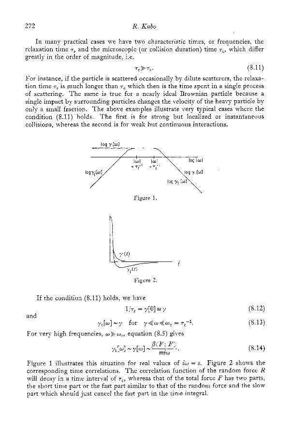
In many practical cases we have two characteristic times, or frequencies, the relaxation time T~ and the microscopic (or collision duration) time T,, which differ greatly in the order of magnitude, i.e.

T p 9 TC’ (8.11)

For instance, if the particle is scattered occasionally by dilute scatterers, the relaxa- tion time T~ is much longer than T~ which then is the time spent in a single process of scattering. The same is true for a nearly ideal Brownian particle because a single impact by surrounding particles changes the velocity of the heavy particle by only a small fraction. The above examples illustrate very typical cases where the condition (8.11) holds. The first is for strong but localized or instantaneous collisions, whereas the second is for weak but continuous interactions.

Figure 1

n

Figure 2.

If the condition (8.11) holds, we have

and l / T r = 7401 = y (8.12)

yt[w] - y for y < w < wc = 7c-1. (8.13)

For very high frequencies, w $ w c , equation (8.5) gives

(8.14)

Figure 1 illustrates this situation for real values of iw = s. Figure 2 shows the corresponding time correlations. The correlation function of the random force R will decay in a time interval of T ~ , whereas that of the total force F has two parts, the short time part or the fast part similar to that of the random force and the slow part which should just cancel the fast part in the time integral.

The jhctuation-dissipation theorem 273

The above considerations show that we may put

if the upper limit is so chosen that T o < r < r r

(8.15)

(8.16)

because the slow tail of the correlation function is cut off. The time integral in equation (8.15) then attains a plateau value for r satisfying (8.16). This fact was noticed by Kirkwood (1946) who first gave equation (8.15) as the microscopic expression for the friction constant of a Brownian particle.

9. Correlation matrix formulation Here we generalize the foregoing treatment of correlation functions to many

variables. We consider a set of physical quantities X1, . . ., X,, which are regarded as stationary stochastic variables fluctuating in equilibrium of the system. It is convenient to normalize the matrix of canonical correlations in such a way that

or

where X ( t ) is a column vector, and k(t) the corresponding row vector, i.e.

Thus (X; k) represents the correlation matrix. This normalization is achieved by diagonalizing the correlation matrix and then changing the norms.

By the stationarity condition of the process X ( t ) we may define a Hermitian matrix C2 by

iQj, = ( i k j ( t ) ; xk(t)) = - (xj(t) ; 2,(t)). (9.3) Then the Langevin equation for X ( t ) is written as a matrix equation

(9.4)

which generalizes equation (4.6) to many variables. For the random force we assume

( R ( t ) ) = 0 and ( R ( t ) ; R(to)) = 0 (9 .5 ) corresponding to equations (4.7) and (4.8). Thus, the Fourier-Laplace transforms of canonical correlation functions

Aik[o] = ~omdte- iuL(Xj ( t+ to ) ; Xk ( tO) )

274 R. Kubo

are found from equation (9.4) to be given by the matrix

where

Corresponding to equation (4.14), the correlation matrix of the random force will satisfy the relation

dte-iut(R(t+to); k(t,))

or r(t) = ( ~ ( t + to ) ; R(to)>.

(9.9)

(9.10)

This can be proved in the same way as was done for equation (4.14), only those alterations necessary for matrix formalism being made.

By equation (5.21) of the linear response theory, A(u) as given by equation (9.6) is the admittance matrix defining the linear response

( X ( t ) ) = %A[w] Koeiwt (9.11)

where K = (Kl, ..., K,) is the force, the Zth component Kl being conjugate to the variable A, defined by

A, = x,. (9.12)

Thus equation (9.6) with equation (9.11) represents the first fluctuation-dissipation theorem, whereas equation (9.9) or (9.10) represents the second fluctuation- dissipation theorem. The Langevin equation (9.4) is extended to

by including the external force K(t). This is the equation of motion of the system in the framework of linear response theory.

We may also define the total force F by

or X = iQX( t )+ F(t) (9.14)

(9.15)

in the absence of external forces. In equation (9.14), iQX is regarded as the restor- ing force for the modes X = (Xl, ..., X,) and F(t) is the microscopic force, which consists of the systematic and the random parts. The above terminology is, how- ever, rather conventional, because the normal mode frequencies are determined not only by the matrix S but also by some part of r ( w ) .

The relation (8.3) or (8.4) is easily generalized to correlation matrices of the total force and the random force. If we define

r t [w ] = e-iwt( F(to + t ) ; i ( t , ) ) (9.16)

The Juctuation-dissipation theorem 275

we then have

(9.17)

corresponding to equation (8.4). This shows that r [ w ] and r t [ w ] behave very differently around the proper frequencies of a, but they approach the same limit at very high frequencies. Generally the situation will be more complex than that discussed in the previous section because there may be more than two character- istic time constants, so that we may have to distinguish, for instance, the adiabatic, the non-adiabatic or the intermediate effects.

We add here some remarks on the symmetry of the correlation matrices. By combining the properties (6.6) and (6.8) we have, in general,

Ajk(w, H) = ~j ~ k A k j ( ~ , - H) (9.18)

where ej is plus or minus one depending on whether Xj is even or odd by time reversal. In particular, if all E ~ ’ S are equal, equation (9.18) gives the symmetry of A for transposition

A(w, H) = A(w, - H). (9.19)

Since a canonical correlation function of real quantities is real, we have the symmetry

-

and (9.20)

(9.21)

Combined with (9.19), the above-mentioned symmetry implies that

~ A n s ( w , H ) = 9 A n , ( - w , H ) = 9 2 A n , ( w , -H)

YA,(w, H) = - 3 A , ( - w , H) = 4 A , ( w , - H)

9 A a ( w , H) = 9 A a ( - U , H) = -%A,(u, - H)

9 A n , ( w , H) = -$A,( - U , H) = -$A,(co, - H) (9.22)

for the symmetric and the antisymmetric parts of the matrix A defined by - A, = &(A+A), A, = &(A-A).

The same symmetry holds for r [ w ] and r i [ w ] because they are related to A(w) by equations (9.7) and (9.17). If we write

rst = 8rs, rS” = sr,

and

rs’, rs”, I’,’ and Fa’’ are all Hermitian. r,’ and Fa’ act as damping coefficients, whereas rs” and r,” result in frequency shifts. Each term has its own even-odd symmetry with respect to w and H as indicated by (9.22).

276 R. Kubo

10. Moments, sum rules and continued fraction expansion We have seen in $ 5 that an admittance is generally expressed in the form

X ( W ) = [o-m+(t) e-iwt dt = ~ ’ ( w ) - i x”(w) . (10.1)

Depending on whether +(t) is even or odd in t , this equation is inverted as

~ ’ ( w ) eiWt dw (10.2)

or as

If the time derivatives exist for +(t) at t = 0, we then have

I ” x’(w) w2?L dw = ( - )” 4 ( 2 ? L ) ( O ) 7-r --m

for an even + and

for an odd 4, in which case another equation

(10.3)

(10.4)

(10.5)

(10.6)

should also be quoted. This last equation is obtained as a particular case of the well-known Kramers-Kronig relation or by applying equation (10.4) to

Generally, ~ ’ ( w ) or ~ ” ( w ) in these equations is positive because it represents the dissipative part of the admittance. On the right-hand sides of the equations we have the derivatives of a response function evaluated at t = 0, which are canonical correlations such as

dBll(0) = P G m ; W)) = ((W, W)) $BA(O) = P<A(O); m) = ((A(O), B(O))) M O ) = p(A(0); B(O)) = - ((A(O), A(() ) ) ) bj,,(O) = -p(A(o) ; B ( 0 ) ) = - { ( A ( O ) , B ( O ) ) ) (10.7)

and so forth. This is summarized by the general sum-rule theorem (Kubo 1957, 1959) which

states that the moments of the frequency distribution of dissipative intensities sum- rule moments are determined by the equilibrium (static) fluctuation of relevant physical quantities. The right-hand sides of equation (10.7) may be just a universal constant determined by the commutation rules of dynamical variables, in which case the sum rule becomes most impressive and useful.

The jhctuation-dissipation theorem 277

Equation (10.1) may be transformed by partial integration to

which is useful at high frequencies. If the expansion is carried out to infinite order, this becomes an asymptotic expansion expressed only in terms of the sum-rule moments, or the sum-rule quantities. This may be called a sum-rule expansion.

There exists another type of moment expansion in the form of a continued fraction which was investigated recently by Mori (1965 b). For simplicity, let us illustrate this for a pair of variables, say X’ and X ” , which represent an oscillatory mode and so form a set of canonical conjugates. We may then take a complex variable

A = X’+iX’’.

I n the absence of a magnetic field, X ‘ and X” differ under time reversal symmetry, so that correlations of the type (A ; A) or (A* ; A*) vanish identically. Then the Langevin equation (9.4) may be written as

A(t) = i w o A ( t ) - y,(t-t’)A(t’)dt’+A,(t), t > t , (10.9)

where A,(t) is a complex random force with the same symmetry as A(t). T h e equation of motion of A,(t) may be put in the same form as equation (10.9) intro- ducing a higher order random force A,(t). Repeating this process, we have a hierarchy of generalized Langevin equations in the form

!11

A,(t) = iw, A,(t) - ~ ~ + ~ ( t - t ’ ) A,(t’) dt’ + A,,+l(t), t > to (10.10) ? t i

with A,( t ) = A( t )

and

(10.11)

(10.12)

(10.13)

These recurrence formulae define the continued fraction

[om dt eciwf( A( t + to) ; A* ( t o ) )

- - (A ; A*>__--. __ (10.14) i ( w -U,) +A,[;(, - wl) + h 2 / ( i ( w - w 2 ) + ...)I-’

where

19

(10.15)

278 R. Kubo

The constants appearing in equation (10.14) are expressed in terms of initial values A,(t,), A,(t,), ..., or, by the recurrence formula (10.10), in terms of the initial derivatives of A(t), namely in terms of the sum-rule moments.

The continued fraction expansion of the type (10.14) includes perturbational calculations, but it is not limited to the category of perturbation. Mori (1965 b, 1966) used this method to investigate the anomaly of transport coefficients of a system near the critical transition. This method is closely related to modern aspects of many- body problems.

11. Density response, conduction and diffusion In order to illustrate the general theory hitherto described, we discuss here the

density response and related subjects for a system of interacting particles. The particle density at a given position is defined by

n(r, t ) = c qr- rl(t)) 2

= nk(t) exp (ik . r) (11.1) k

where nk(t) is the Fourier component

nk( t ) = L-3 C exp { - ik . r2(t)} 1

(11.2)

L3 being the volume of the space, and similarly the current density and its Fourier components are defined by

j ( r , t ) = jk(t)exp(ik.r) (11.3)

(11.4)

k

1 1 m

jk(t) = L-3 2 - [p2(t) exp { - i k . r2(t)}].

The density and current Fourier components have the Poisson bracket

(11.5) n . (j -k , %) = mzk

where n is the number density of the particle. The continuity equation is written as

hk(t)+ik.jk(t) = 0. (11.6)

When an external potential pe(r, t ) is imposed the perturbation is given by the

= c n-k(t) pke(t) (11.7)

where pke(t) is the spatial Fourier component of the external potential. Then the linear response of the system to

is expressed by

for the density, and by

Hamiltonian

k

pke( t ) = Wpke eiWt

(nk(t)) = - 9x[k, W ] pke eiot

(jk(t)) 1 - 9 p [ k , W ] ikpk" eiWt

(11.8)

(11.9)

The juctuation-dissipation theorem

for the current, where

x [ k , w ] = Jocdt e-i"'((n-k(0), nk( t ) ) )

(see equation (5.166)) is the susceptibility for the density response and "cc

,ue[k, w] = /3! dt e-i"f(j-k(0); j k ( t ) ) 0

279

(1 1.10)

(11.1 1)

is the external mobility tensor (see equations (5.21) and (11.6)). This terminology is introduced here in order to discriminate it from the local mobility p which will be defined later. The susceptibility and the external mobility are related with each other by equation (7.3), namely

iwx[k, U ] - k . p e [ k , w ] . k = 0 (1 1.12)

which is also obtained from equation (1 1.10) by performing partial integration. N o w let us consider the canonical correlation of density fluctuation

(n-k(o) ; nk(t)) and define its Fourier-Laplace transform

A [ k , W ] = dt e-iut(n-k(0); nk(t)) I O W (1 1.13)

which is related to the susceptibility by

(1 1.14)

as is easily proved by partial integration of the right-hand side of equation (11.13) with the use of equation (5.20). Here x ( k , 0) is the static density susceptibility to the external potential Pke, namely

1 N k , U1 = 7 (x[k , 01 - x [ k , W I )

zwP

x [ k , O ] = /3(n-k(o); nk(o)) = -~ (1 1.15) 8pke which approaches, as k+O,

(11.16)

where ( is the chemical potential and K the isothermal compressibility. The first equality in equation (11.16) is obtained by identifying the local change of -pe with that of the chemical potential. The second equality follows from the Gibbs- Duhem relation.

We now write A [ k , w ] , equation (1 1.13), in the form

(1 1.17)

A s we have seen in 5 7, equation (1 1.6) is then regarded as a Langevin equation

&(t) = - i k . j k o ( t ) - i k . j k ' ( t ) (1 1.18)

280 R. Kubo

where the systematic current jko(t) is defined by the equation

and

is the random current. The systematic current is the part of the total current jk(t) induced by the density change. Equation (11.18) corresponds to equation (8.1) or (10.9) (with wo = 0), so that the second fluctuation-dissipation theroem, (7.16) or ( lO, l l ) , tells us that the function Yk[w] in equation (11.17) is determined by the time correlation of the random current. Thus we may write it as

(11.21)

where the local mobility tensor is defined by m

p*[k, w ] = /3j dt e-iwt(j-i(0); jk'(t)) (1 1.22) 0

and the diffusion constant D by

D[k, w ] = p*P, wl/x[k, 01. (1 1.23)

Equation (8.3) is applied here to obtain the relationship between the external and local mobilities, which amounts to

or

(1 1.24)

(1 1.25)

In the last equation we introduced the shielding factor E*[k, w ] by the definition

(1 1.26)

(1 1.27)

by virtue of equations (11.24) and (11.12). It is remarked incidentally that the shielding factor c*[k, w ] or the susceptibility

x[k, w ] has a close relation with the thermodynamic property of the particle system. If the particles interact with a pair potential

E(Y - Y') = dk Z'k exp {ik. (r - r')] J the total interaction energy is

Eint = iL3 z'k n-k f i k . k

(1 1.28)

The jluctuation-dissipation theorem 281

Then we have for the free energy F of the system the relationship

(1 1.29) 1 7~ i'" 1 -e-pnw O1 (c*[k,w])*

a~ 2-- = (n-knk) = - dw---$ ____ zvk L3 This is an example of application of the fluctuation-dissipation theorem in the form of equation (6.15), which gives for x[k, w] the equation

l-e-pfiw m 23x[k,w] = - 1- (%k( 0 ) nk( t ) ) e-iwt dt . (1 1.30)

Reversing the transformation for t = 0 and using equation (11.27), we arrive at equation (1 1.29). This equation is sometimes called the dielectric formula? (Nozieres and Pines 1958, Englert and Brout 1960), and it allows computation of the free energy, or the ground-state energy in particular, using a certain approximation for the shielding function E*[k, U]. As an additional remark, we note that the integral on the right-hand side of equation (11.30) is known as the dynamic form factor S[k, w], which is thus expressed in terms of the shielding factor or the susceptibility function. The generalized diffusion constant D[k,w] is thus related to the dynamic form factor which is observable, for instance, by neutron inelastic measurements.

It is essentially the real part of A[k,w].

The current response (11.9) may be written as ( jk ( t ) ) = - Wp*[k, U] ikpkmeiwt (1 1.31)

where the potential pk*(t) of the local field is introduced by the definition

(11.32) 1 pk*(t) = E*[k,J p k e ( t ) *

This can be written, with the use of equations (11.27), (11.8) and (11.1.5), as

(1 1.33)

which shows that the local field is the resultant of the external field and the effective field induced by the density change. The latter causes the shielding of the applied field. The current may be supposed to be driven either by the external field with the external mobility pe[k ,w] or by the local field with the local mobility ,u*[k,w] (Luttinger 1964, Martin 1965).

As long as the particle interaction is short-ranged, it can generally be proved that the static susceptibility x[k, 01-1 is non-singular at k = 0, so that the local field correction vanishes in the long wavelength limit k+O, i.e.

lim E*[k, w] = 1 k+O

(1 1.34)

if the particles are not bound, and so the local mobility should remain finite at k = 0 and w = 0. Therefore the external and local mobilities become equal in the limit k + 0, and equation (1 1.23) gives the Einstein relation

D=D[O, 01 = p y 0 , 01 . /E (11.35)

7 Usually the dielectric formula is written in terms of the dielectric function c[k, w ] defined by equation (1 1.40) rather than the shielding factor.

282 R. Kubo

For small non-zero k’s , equation ( 1 1 . 3 3 ) may be approximated by

(1 1.36)

which means that the local field correlation is nothing but the chemical potential change induced by the density change. This appears as the diffusion force or the pressure gradient.

For charged particles the function x[k, 01-l is singular at k = 0 in such a way that

4ne2 k2 x[k, O]-’N--- (1 1.37)

is the dominant term for small A’s, e being the charge on each particle. This comes from the Coulomb interaction energy which contributes a part of the free energy change when a density fluctuation is induced with a wave number k. If we take only this term of x[k, 01-l to define the local field

(11.38)

the shielding factor becomes equal to the usual dielectric constant E[k,w]. It should be remembered, however, that the shielding factor E*[k, w ] as defined by (11.25) generally differs from the dielectric constant because the local field in equation (11.33) contains, in principle, all sorts of local effects such as diffusion, pressure gradient and even thermoelectric force.

For charged particles it is customary to talk about the conductivity defined by

(1 1.39) o[k, w ] = e2 p*[k, w]

in terms of which equation (1 1.26) is written as

477 E[k, U ] = 1 +? k . o[k, U]. k zwk2

( 1 1.40)

which is a familiar expression for the dielectric constant in terms of the conduc- tivity. T h e conductivity tensor o is therefore given by equation (11.22), namely

o[k, w ] = e z ~ ~ o ~ d ~ e - ~ w t ( j ~ k ’ ( 0 ) ; j i ( t ) ) (1 1.41)

in terms of the correlation function of the random current. This should be discriminated from the expression of the external conductivity

m oe[k, w] = e2p/ dte-lwt(j_,(0); jk(t))

0

which is related to o[k, w ] by

Note, however, that these equations may fail for large k’s for tion (11.37) is no longer valid.

(1 1.42)

(1 1.43)

which the approxima-

The fluctuation-dissipation theorem 283

The sum-rule consideration can be applied to both kinds of conductivity, although it becomes more complicated for the local conductivity. The lowest-order sum rule equally applies to both, for the random current is initially equal to the total current. Therefore we have

ne2 m 1 /a Wo[k, U ] dw = goe[k, w ] dw = --. = - m

(1 1.44)

Within the framework of the linear response theory, all the necessary informa- tion about the system is contained in the function A[k, w] or x[k, w ] or any of the related quantities. I n the spirit of the fluctuation-dissipation theorem this means that any one of these functions tells us all possible modes of collective oscillation, individual excitations around the equilibrium states, etc. I n particular, at low frequencies and for long wavelengths the macroscopic or hydrodynamical laws governing the motion of the system are directly reflected in the structure of these response functions (Kadanoff and Martin 1963). This means that the transport or the kinetic coefficients appearing in the hydrodynamic equations can be identified with proper microscopic expressions when the response functions are calculated by statistical mechanics. A simple example has been given here for the conduc- tivity. Such expressions are very fundamental for the statistical-mechanical theory of irreversible processes and have proved very useful for practical computations. The great advantage is that they, are valid even when the traditional kinetic equation method is questionable or cannot be used. On the other hand, one should, of course, appreciate the great power of kinetic equations within their own limitations as they are able to cover a large area of non-linear phenomena. Extension of the present approach to the non-linear rCgime is possible (Bernard and Callen 1959) but it has not been explored to any great extent. Further discussion of applications and extensions is out of place in the present article.

References BERNARD, W., and CALLEN, H. B., 1959, Rea. Mod. Phys., 31, 1017. CALLEN, H. B., and GREEXE, R. F., 1952, Phys. Rea., 86, 702; 88, 1387. CALLEN, H . B., and WELTON, T. A., 1 9 5 1 , Phys. Rea., 83, 34. CHANDRASEKHAR, S . , 1943, Rea. Mod. Phys., 15, 1 . CHESTER, G. V., 1963, Rep. Progr. Phys., 26, 411 (London: Institute of Physics and Physical

EINSTEIS, A., 1905, Ann. Phys., Lpz., 17, 549. ENGLERT, F., and BROUT, R., 1960, Phys. Rea., 120, 1085. GREEN, RI. S. , 1952,J. Chem. Phys., 20, 1281. __ 1954,J. Chem. Phys., 22, 398. KADANOFF, L. P., and MARTIN, P. C., 1963, Ann. Phys., A'. Y., 24, 419. KIRKWOOD, J., 1946, J. Chem. Phys., 14, 180. KUBO, R., 1957,J. Phys. Soc,Japan, 12, 570. __ 1959,Lecturesin Theoretical Physics,Vol. 1 , Ed. W. Brittin(NewYork: inter science),^. 120. __ 1965, Statistical lllechanics of Equilibrium and Non-equilibrium, Ed. J. Aleixner (Amster-

__ 1966, Tokyo Summer Lectures in Theoretical Physics, 1965, Part I, 1Wany-Body Theory,

KUBO, R., and TOMITA, K., 1954,J. Phys. Soc.Japan, 9, 888. LUTTINGER, J. AI. , 1964, Phys. Rea., 135, Al505,

Society).

dam: North-Holland), p. 80.

Ed. R. Kubo (Tokyo: Shokabo; New York: Benjamin).

284 R. Kubo

MARTIN, P. C., 1965, Statistical Mechanics of Equilibriunz and Non-equilibrium, Ed. J. Meixner

MORI, H., 1956,J. Phys. Soc.Japan, 11, 1029. - 1965 a, Progr. Theor. Phys.,Japan, 33, 423. - 1965 b, Progr. Theor. Phys.,Japan, 34, 399. - 1966, Tokyo Summer Lectures in Theoretical Physics, 1965, Part I, Many-Body Theory,

NAKANO, H., 1956, Progr. Theor. Phys.,Japan, 15, 77. NOZIERES, P., and PIKES, D., 1958, Nuovo Cim., [XI, 9, 470. NYQUIST, H., 1928, Phys. Rev., 32, 110. ONSAGER, L., 1931, Phys. Rev., 37, 405.

UHLENBECK, G. E., and ORNSTEIN, L. S., 1930, Phys. Rev., 36, 823. WANG, M. C., and UHLENBECK, G. E., 1945, Rev. Mod. Phys., 17, 327. ZWANZIG, R., 1965, Annual Revieu: of Physical Chemistry, Vol. 16, Ed. H. Eyring (Palo Alto,

(Amsterdam: North-Holland), p. 100.

Ed. R. Kubo (Tokyo: Shokabo; New York: Benjamin).

TAKAHASHI, H., 1952,J. Phys. S O C . Japan, 7, 439.

California: Annual Reviews, Inc.), p. 67.