The Fizeau Experiment: Experimental Investigations of the...

The African Review of Physics (2013) 8:0043 297

The Fizeau Experiment: Experimental Investigations of the Relativistic Doppler Effect

Anthony Maers1, Richard Furnas2, Michael Rutzke3 and Randy Wayne4,*

1Department of Biological Statistics and Computational Biology, Cornell University, Ithaca, NY, USA 2Department of Mathematics, Cornell University, Ithaca, NY USA

3Robert W. Holley Center, United States Department of Agriculture, Cornell University, Ithaca, NY, USA 4Laboratory of Natural Philosophy, Department of Plant Biology, Cornell University, Ithaca, NY USA

We built a Fizeau interferometer that takes advantage of laser light, digital image capture and computer analysis to reproduce the celebrated experiments of Fizeau, Michelson & Morley, and Zeeman, concerning the optics of bodies in relative motion. Like Fizeau, Michelson & Morley, and Zeeman, we found that the zeroth-order central fringe shifts in a velocity-difference-dependent manner. The experimentally-observed fringe displacement was 0.0419 per m/s. If the fringe shift resulted from the linear addition of the velocity of light in water and the velocity of the water, as predicted by Newtonian kinematic theory, the fringe shift would be 0.0784 per m/s. If the fringe shift resulted from the nonlinear addition of the velocity of light in water and the velocity of water, as predicted by the kinematics of the Special Theory of Relativity, the fringe shift would be 0.0151 per m/s. If the fringe shift resulted from the relativistic Doppler-induced transformation of the wavelength of light flowing with and against the water, the fringe shift would be 0.0441 per m/s. We found that the magnitude of the experimentally-observed fringe shift is most accurately accounted for by considering the moving water to cause a relativistic Doppler-induced change in the wavelength of light.

1. Introduction

Einstein [1] considered Fizeau’s aether drag experiment to be an experimentum crucis in deciding between the Newtonian velocity addition law, which is based on absolute time, and the velocity addition law consistent with Special Theory of Relativity, which is based on the relativity of time. The Fizeau experiment [2-4] measured the effect of moving water on the interference pattern produced by two beams of light—one moving parallel to the water velocity and the other moving antiparallel to the water velocity. Fizeau found that the observed displacement of the interference pattern was smaller than that that predicted to occur if the velocity of the water through which the light propagated was simply added to the velocity of light traveling parallel with the water and simply subtracted from the velocity of light traveling antiparallel to the water. The conclusion that the velocities were not simply additive were confirmed by the celebrated experimentalists, Michelson & Morley [5] and Zeeman [6,7]. _______________ *[email protected]

Von Laue [8] interpreted the lack of simple additivity of the velocities consistent with Newtonian kinematic theory to be a direct consequence of the relativity of time posited by the Special Theory of Relativity. Einstein [1] wrote that the Fizeau experiment “decides in favour of [the velocity addition law] derived from the theory of relativity, and the agreement is, indeed, very exact. According to recent and most excellent measurements by Zeeman, the influence of the velocity of flow v on the propagation of light is represented by [the velocity addition law] to within one percent”. Recently, Lahaye et al. [9] described the Fizeau experiment as “a crucial turning point between old and modern conceptions of light and space-time” and they “believe this makes its replication particularly valuable from a pedagogical point of view.”

In a paper published in this journal, Mears and Wayne [10] showed that the magnitude of the fringe shifts observed by Fizeau, Michelson & Morley, and Zeeman could be accounted for in terms of absolute time by considering the beam of light traveling parallel to the water was to be red-shifted by the Doppler effect and the beam of light traveling antiparallel to the water was to be blue-shifted by the Doppler effect. This explanation accounts for the combined results obtained by


Fizeau, Michelson & Morley, and Zeeman with greater than twice the accuracy than the explanation given by the Special Theory of Relativity [10]. Curiously, even though the Doppler Effect is readily perceived when there is relative motion, standard theories rarely, if ever, include the Doppler effect as a primary consideration in the study and description of relative motion. Our work is unique in that it incorporates the relativistic Doppler Effect from the beginning. When expanded to second order, the inclusion of the Doppler effect makes it possible to unify many aspects of mechanics, electrodynamics and optics that are usually treated separately. Indeed, the Doppler effect expanded to second order combined with absolute time also provides alternative derivations of results familiar from the Special Theory of Relativity describing the relativity of simultaneity [11], the arrow of time [12], and why charged particles cannot exceed the vacuum speed of light [13].

The Special Theory of Relativity explains the results of the Fizeau experiment using kinematics as opposed to the theory proffered by Maers and Wayne that explains the results of the Fizeau experiment as a velocity-induced transformation of waveforms [14] that result from the relativistic Doppler effect. Here we have reconstructed the Fizeau experiment using a laser, a video camera, image processing software and computer-assisted analysis. Our results confirm that the theory proffered by Mears and Wayne [10] accounts for the experimental results of the Fizeau experiment more accurately than does the Special Theory of Relativity.

2. Materials and Methods

Construction of the interferometer. This interferometer, like that built by Lahaye et al. [9], is simple and inexpensive enough to be used in high school and undergraduate physics laboratories or in science fairs. We constructed an interferometer based on Michelson & Morley’s design [5] except that the prism used in their interferometer was replaced with mirrors (Figs. 1 and 2). A 532 nm green laser pointer (Model 10098; xUMP.com) provided the light source. The laser was leveled by measuring the height of the laser beam as we projected it across the laboratory.

The laser light was shaped by an adjustable slit (Model 125096; Proindustrial.com) and was directed onto a beam splitter composed of a two inch by two inch half-silvered glass plate with 50% transmission and 50% reflection (Part # 45-854; Edmund Optics). The beam splitter was mounted on a two inch by two inch kinematic mount (Part # 58-861, Edmund Optics, Barrington, NJ USA). The

four optically flat �� front surface mirrors 12.7 mm

in diameter (Part # 43-400533; Edmund Optics, Barrington, NY USA) were each mounted on a 0.5 inch diameter three screw kinematic mount (Part # 58-853; Edmund Optics). Mirrors 1 and 4 were oriented 67.5 degrees relative to the plane of the half-silvered mirror. Mirrors 2 and 3 were oriented 45 degrees relative to the plane of the half-silvered mirror. The light in the interferometer propagated through copper tubes (½ inch L Mueller copper tube available from local hardware stores). The tubes were five feet long with an internal diameter of 1.27 cm. The two tubes were terminated on all ends with ½ inch to 1¼ inch diameter couplers and 1¼ inch diameter T-junctions to minimize the flow reductions due to the turns. A flat brass ½ inch-hole washer was welded on the terminal end of each T-junction. On one end of the two pipes, the two T-junctions were welded together with a copper tube so that the tubes formed a “U” shape and the two arms of the “U” were approximately 9.5 cm apart. The T-junctions at the ends of the tubes were closed with 3.3 mm thick BOROFLOAT windows (Part # 48-543; Edmund Optics) secured to the brass washers with Loctite 5 min quickset epoxy (Henkel Corp, Rocky Hill, CT USA). We mixed the epoxy and let it sit for approximately four minutes before spreading a thin yet complete layer around the outside of the brass washers. We then strongly pressed on the window and held the window firmly while maintaining pressure for five minutes to allow the epoxy to cure. We had to be careful not to let the epoxy seep too much into the window area or this would disrupt the laser's path. The ends of the copper tubes were approximately 1 cm from the glass windows. This adds some uncertainty on the order of 0.1% in determining the actual optical path length of the flowing water in the interferometer tubes. The tubes of the interferometer were mounted on a two meter long optical rail (Oriel Corp., Stratford, CT USA).

The African Review of Physics (2013) 8

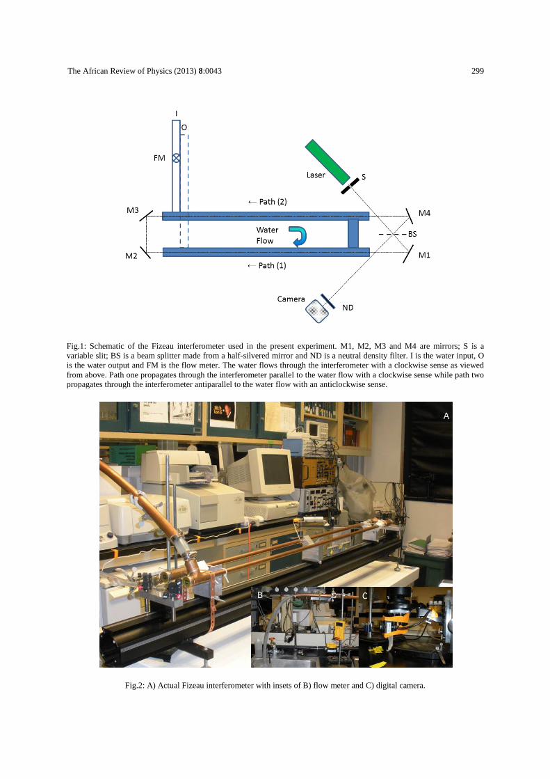
Fig.1: Schematic of the Fizeau interferometer used in the present experiment. M1, M2, M3 and M4 are mirrors; variable slit; BS is a beam splitter made from a halfis the water output and FM is the flow meter. from above. Path one propagates through the interferometer parallel to the water flow witpropagates through the interferometer antiparallel to the water flow with an anticlockwise sense.

Fig.2: A) Actual Fizeau interferometer with

8:0043

Schematic of the Fizeau interferometer used in the present experiment. M1, M2, M3 and M4 are mirrors; BS is a beam splitter made from a half-silvered mirror and ND is a neutral density filter. I is the water input, O

is the water output and FM is the flow meter. The water flows through the interferometer with a clockwise sensepropagates through the interferometer parallel to the water flow with a clockwise sense while path two

propagates through the interferometer antiparallel to the water flow with an anticlockwise sense.

Fizeau interferometer with insets of B) flow meter and C) digital camera

299

Schematic of the Fizeau interferometer used in the present experiment. M1, M2, M3 and M4 are mirrors; S is a silvered mirror and ND is a neutral density filter. I is the water input, O

r with a clockwise sense as viewed h a clockwise sense while path two

of B) flow meter and C) digital camera.


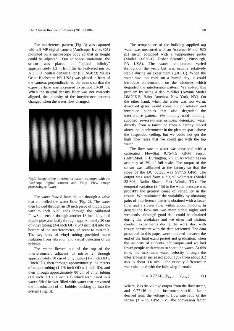
The interference pattern (Fig. 3) was captured with a 9 MP digital camera (AmScope, Irvine, CA) mounted on a microscope body so that its height could be adjusted. Due to space limitations, the sensor was placed at “optical infinity” approximately 1.3 m from the half-silvered mirror. A 2 O.D. neutral density filter (03FNG023; Melles Griot, Rochester, NY USA) was placed in front of the camera; perpendicular to the beams so that the exposure time was increased to around 10-30 ms. When the neutral density filter was not correctly aligned, the intensity of the interference patterns changed when the water flow changed.

Fig.3: Image of the interference pattern captured with the AmScope digital camera and Toup View image processing software.

The water flowed from the tap through a valve that controlled the water flow (Fig. 2). The water then flowed through an 18 inch piece of nipple pipe with ½ inch NPT ends through the calibrated FlowStat sensor, through another 18 inch length of nipple pipe and lastly through approximately 50 cm of vinyl tubing (3/4 inch OD x 5/8 inch ID) into the bottom of the interferometer, adjacent to mirror 3. The segments of vinyl tubing provided some isolation from vibration and visual detection of air bubbles.

The water flowed out of the top of the interferometer, adjacent to mirror 2, through approximately 10 cm of vinyl tubes (1¼ inch OD x I inch ID), then through approximately 1½ meters of copper tubing (1 1/8 inch OD x 1 inch ID), and then through approximately 80 cm of vinyl tubing (1¼ inch OD x 1 inch ID) which terminated in a water-filled beaker filled with water that prevented the introduction of air bubbles backing up into the system (Fig. 3).

The temperature of the building-supplied tap water was measured with an Accumet Model 925 pH meter equipped with a temperature probe (Model 13-620-17; Fisher Scientific, Pittsburgh, PA USA). The water temperature varied throughout the year, but was usually relatively stable during an experiment (±0.1 C). When the water was too cold, on a humid day, it could introduce condensation on the windows which degraded the interference pattern. We solved this problem by using a dehumidifier (Amana Model DM70E-E; Haier America, New York, NY). On the other hand, when the water was too warm, dissolved gases would come out of solution and introduce bubbles that also degraded the interference pattern. We initially used building-supplied reverse-phase osmosis deionized water directly from a faucet or from a carboy placed above the interferometer in the plenum space above the suspended ceiling, but we could not get the high flow rates that we could get with the tap water.

The flow rate of water was measured with a calibrated FlowStat 0.75-7.5 GPM sensor (InstruMart, S. Burlington, VT USA) which has an accuracy of 2% of full scale. The output of the sensor was calibrated at the factory so that the slope of the DC output was 5V/7.5 GPM. The output was read from a digital voltmeter (Model 22-806; Radio Shack, Fort Worth, TX). The temporal variation (± 4%) in the water pressure was probably the greatest cause of variability in the results. We minimized the variability by obtaining pairs of interference patterns obtained with a faster flow and a slower flow within about 30-60 s. In general the flow rate was more stable nights and weekends, although good data could be obtained during the weekdays and we often had visitors conduct experiments during the work day, with results consistent with the data presented. The data presented in this paper were obtained between the end of the final exam period and graduation, when the majority of students left campus and we had fewer people with whom to share the water. At this time, the maximum water velocity through the interferometer increased about 12% from about 3.2 m/s to about 3.6 m/s. The velocity difference � was calculated with the following formula:

� = 0.77146(�� −��) (1) Where, � is the voltage output from the flow meter, and 0.77146 is an instrument-specific factor derived from the voltage to flow rate ratio of the sensor (� =7.5 GPM/5 V), the conversion factor


� = ��

�.�� !"#$��"�%

�&�� needed to convert GPM

to m3/s, and the cross sectional area ' = 1.2267 × 10-4 m2 of the copper pipe in the interferometer. The constant that relates the velocity difference to the voltage difference is:

)*+ = 0.77146 (2)

The flow can be described by its Reynolds Number ,-:

,- ≈ /012 (3)

Where, � varied from 0 to 3.6 m/s, the water density 3 =103 kg/m3, the characteristic length or diameter of the pipe 4 = 2.54 × 10-2 m and the viscosity of the water 5 = 0.001 Pa s. The Reynolds Numbers that describe the flow of water through the pipes in the interferometer vary from ,- ≈12,700 for flows of 0.5 m/s to ,- ≈91,440 for flows of 3.6 m/s. These Reynolds Numbers are all greater than 2,300, indicating that the flow is turbulent [15]. Fizeau [4], Michelson & Morley [5], Zeeman [7] and Lahaye et al. [9] estimate that the ratio of the maximal velocity where the light beams propagate to the average velocity that is measured is approximately equal to 1.16. Consequently, the predicted theoretical fringe shifts for a given measured velocity have been multiplied by 1.16.

The pattern of the water flow is not simple. In principle, it would be possible to construct models that could predict some of the effects of accelerations around the corners of the interferometer, however, despite the significant effort that would be required; the residual uncertainty is still likely to be unacceptable to apply as a correction to the experiment. Consequently, we accept our ignorance concerning localized accelerations and consider the velocities to be constant in the straight sections of tube through which the light beams travelled.

Method of alignment. Before aligning the interferometer, we let the tap water run for at least half an hour to allow the system to stabilize. We aligned the interferometer while water was running through it with a velocity of approximately 1.5 m/s. One of the light paths was blocked by placing a card in front of either mirror 1 or mirror 4. This allowed us to isolate one light path at a time. From here we could align both the (1) clockwise and (2) anticlockwise light paths independently. Light propagating along path (1) propagated through the half-silvered mirror to mirror 1, to mirror 2, to

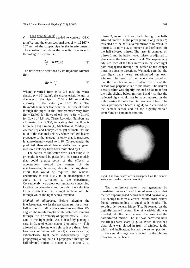
mirror 3, to mirror 4 and back through the half-silvered mirror. Light propagating along path (2) reflected off the half-silvered mirror to mirror 4, to mirror 3, to mirror 2, to mirror 1 and reflected off the half-silvered mirror. The laser is centered on mirror 1 and the half-silvered mirror is adjusted to also center the laser on mirror 4. We sequentially adjusted each of the four mirrors so that each light path propagated through the center of the copper pipes in opposite directions. We made sure that the two light paths were superimposed on each window. The sensor of the camera was placed so that the two beams were centered on it and the sensor was perpendicular to the beam. The neutral density filter was slightly inclined so as to reflect the light slightly below mirrors 1 and 4 so that the reflected light would not be superimposed on the light passing through the interferometer tubes. The two superimposed beams (Fig. 4) were centered on the camera sensor and on the digitally-marked center line on computer monitor.

Fig.4: The two beams are superimposed on the camera sensor and on the computer monitor.

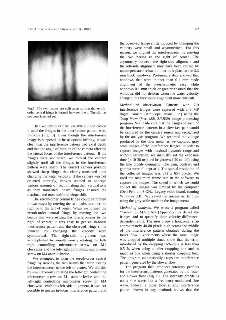
The interference pattern was generated by translating mirrors 1 and 4 simultaneously so that the two superimposed beams separated horizontally just enough to form a vertical zeroth-order central fringe, corresponding to equal path lengths. The zeroth-order central fringe (Fig. 5) formed on the digitally-marked central line. A variable slit was inserted into the path between the laser and the half-silvered mirror. The slit was narrowed until the fringes were sharp (Fig. 3). When an inclined glass plate was placed in front of window 4, the width and inclination, but not the center position, of the central fringe was affected by the oblique refraction of the beam.


Fig.5: The two beams are split apart so that the zeroth-order central fringe is formed between them. The slit has not been inserted yet.

Then we introduced the variable slit and closed it until the fringes in the interference pattern were in-focus (Fig. 3). Even though the interference image is supposed to be at optical infinity, it was clear that the interference pattern had axial depth and that the angle of rotation of the camera affected the lateral focus of the interference pattern. If the fringes were not sharp, we rotated the camera slightly until all the fringes in the interference pattern were sharp. The correct camera position showed sharp fringes that clearly translated upon changing the water velocity. If the camera was not oriented correctly, fringes seemed to undergo various amounts of rotation along their vertical axis as they translated. Sharp fringes ensured the maximal and most uniform fringe shift.

The zeroth-order central fringe could be formed in two ways: by moving the two paths to either the right or to the left of center. When we formed the zeroth-order central fringe by moving the two beams that were exiting the interferometer to the right of center, it was easy to get an in-focus interference pattern and the observed fringe shifts induced by changing the velocity were symmetrical. The right-side alignment was accomplished by simultaneously rotating the left-right controlling micrometer screw on M1 clockwise and the left-right controlling micrometer screw on M4 anticlockwise.

We attempted to form the zeroth-order central fringe by moving the two beams that were exiting the interferometer to the left of center. We did this by simultaneously rotating the left-right controlling micrometer screw on M1 anticlockwise and the left-right controlling micrometer screw on M4 clockwise. With this left-side alignment, it was not possible to get an in-focus interference pattern and

the observed fringe shifts induced by changing the velocity were small and asymmetrical. For this reason, we aligned the interferometer by moving the two beams to the right of center. The asymmetry between the right-side alignment and the left-side alignment may have been caused by uncompensated refraction that took place at the 3.3 mm thick windows. Preliminary data showed that windows that were thinner than 0.1 mm made alignment of the interferometer easy while windows 0.1 mm thick or greater ensured that the windows did not deform when the water velocity changed, but they made alignment more difficult.

Method of observation. Patterns with 7-9 interference fringes were captured with a 9 MP digital camera (AmScope, Irvine, CA) using the Toup View (Ver. x86, 3.7.939) image processing program. We made sure that the fringes in each of the interference patterns in a slow-fast pair would be captured by the camera sensor and recognized by the analysis program. We recorded the voltage produced by the flow meter as we captured gray scale images of the interference fringes. In order to capture images with maximal dynamic range and without saturation, we manually set the exposure time (≈ 10-30 ms) and brightness (-20 to -40) using the line profile command. The gain, contrast and gamma were all kept at 1. The spatial resolution of the collected images was 872 x 654 pixels. We used the maximum frame rate in the software to capture the images. The speed in which we could collect the images was limited by the computer (Dell Pentium 3 GHz, Legacy video board, running Windows XP). We saved the images as .tif files using the gray scale mode in the Image menu.

Method of analysis. We wrote a program called “ fizeau” in MATLAB (Appendix) to detect the fringes and to quantify their velocity-difference-dependent shift. The user crops a horizontal strip approximately 40-80 pixels high across the middle of the interference pattern obtained during the faster flow. Experiments where the same image was cropped multiple times show that the error introduced by the cropping technique is less than 0.5 % when using a taller cropping box and as much as 1% when using a shorter cropping box. The program automatically crops the interference pattern generated by the slower flow.

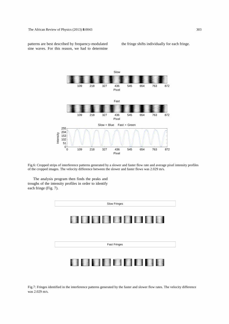
The program then produces intensity profiles for the interference patterns generated by the faster and slower flow (Fig. 6). The intensity profile is not a sine wave, but a frequency-modulated sine wave. Indeed, a close look at any interference pattern shown in any textbook shows that the


patterns are best described by frequency-modulated sine waves. For this reason, we had to determine

the fringe shifts individually for each fringe.

Fig.6: Cropped strips of interference patterns generated by a slower and faster flow rate and average pixel intensity profiles of the cropped images. The velocity difference between the slower and faster flows was 2.029 m/s.

The analysis program then finds the peaks and troughs of the intensity profiles in order to identify each fringe (Fig. 7).

Fig.7: Fringes identified in the interference patterns generated by the faster and slower flow rates. The velocity difference was 2.029 m/s.

0 109 218 327 436 545 654 763 8720

51102153204255

Pixel

Inte

nsity

Slow = Blue Fast = Green

Slow

Pixel109 218 327 436 545 654 763 872

Fast

Pixel109 218 327 436 545 654 763 872

Slow Fringes

Fast Fringes


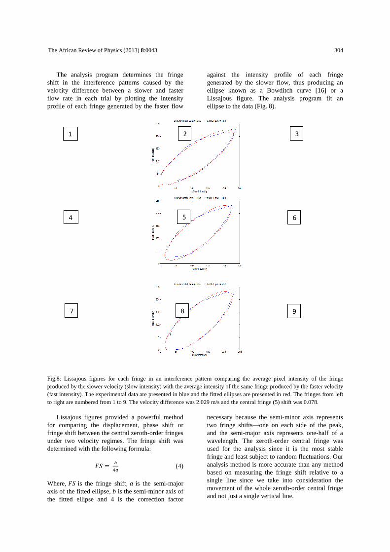
The analysis program determines the fringe shift in the interference patterns caused by the velocity difference between a slower and faster flow rate in each trial by plotting the intensity profile of each fringe generated by the faster flow

Fig.8: Lissajous figures for each fringe in an interference pattern produced by the slower velocity (slow intensity) (fast intensity). The experimental data are presented in blue and the fitted ellipses are presented in red. to right are numbered from 1 to 9. The velocity difference was

Lissajous figures provided a powerful method for comparing the displacement, phase shift or fringe shift between the central zerothunder two velocity regimes. The fringe shift was determined with the following formula:

67 = 8$� Where, 67 is the fringe shift, 9 is the semiaxis of the fitted ellipse, : is the semithe fitted ellipse and 4 is the correction factor

1

4

7

8:0043

The analysis program determines the fringe shift in the interference patterns caused by the velocity difference between a slower and faster

by plotting the intensity profile of each fringe generated by the faster flow

against the intensity profile of each fringe generated by the slower flow, thus producing an ellipse known as a Bowditch curve [Lissajous figure. The analysis program fiellipse to the data (Fig. 8).

for each fringe in an interference pattern comparing the average pixel intensity (slow intensity) with the average intensity of the same fringe produced

The experimental data are presented in blue and the fitted ellipses are presented in red. The velocity difference was 2.029 m/s and the central fringe (5) shift was 0.078.

provided a powerful method the displacement, phase shift or en the central zeroth-order fringes

The fringe shift was determined with the following formula:

(4)

is the semi-major is the semi-minor axis of

4 is the correction factor

necessary because the semitwo fringe shifts—one on each side of the peak, and the semi-major axis represents onewavelength. The zeroth-order used for the analysis since it is the most stable fringe and least subject to random fluctuations.analysis method is more accurate than any method based on measuring the fringe shift relative to a single line since we take into consmovement of the whole zerothand not just a single vertical

2

5

8

304

against the intensity profile of each fringe generated by the slower flow, thus producing an

pse known as a Bowditch curve [16] or a . The analysis program fit an

the average pixel intensity of the fringe with the average intensity of the same fringe produced by the faster velocity

The experimental data are presented in blue and the fitted ellipses are presented in red. The fringes from left shift was 0.078.

semi-minor axis represents one on each side of the peak,

major axis represents one-half of a order central fringe was

used for the analysis since it is the most stable fringe and least subject to random fluctuations. Our analysis method is more accurate than any method based on measuring the fringe shift relative to a single line since we take into consideration the movement of the whole zeroth-order central fringe

line.

9

6

3


Statistical analysis to compare the slope of the regression equation for the experimental values with the slope of the theoretical equation for the Newtonian theory, the Doppler theory,Special Theory of Relativity was performed with JMP statistical software (version 10.0.2; Institute Inc.).

Theoretical analysis. The predicted given by the following theoretical formulae

Newtonian Theory 67 = 1.16 ∙ �</�=

Special Relativity 67 = 1.16 ∙ �</�=

Doppler Theory 67 = 1.16 ∙ �</�= Where, > is the total length of the tubes (3.048 m), � is the velocity difference between the fast flow and slow flow in a given trial, ? is thof the laser (532 × 10-9 m) , @ is the vacuum speed of light (2.99 × 108 m/s) and A is the refractive index of the flowing fluid. The estimated ratio of the maximal velocity where the light beams propagate to the average velocity that is measured is 1.16. The magnitude of the fringe shift with velocity difference is instrument dependent and depends on the wavelength of lightof the tubes, which represents the amount of interaction between the light and the water.

Fizeau [2-4], Michelson & Morley [5], Zeeman [6,7] and Lahaye et al. [9] have already Newtonian theory cannot explain the results of the Fizeau experiment. What is at stake here is whether the fringe shift resulting from the relative motion of the water and the optical system is best described by Eqn. (6), where time is transforminertial frames traveling at velocity each, or by Eqn. (7), where wavelength is transformed between inertial frames traveling at velocity � relative to each.

3. Results and Discussion

In the interferometer setup used, the the left when the water velocity changes from fast to slow (Fig. 9).

8:0043

Statistical analysis to compare the slope of the regression equation for the experimental values with the slope of the theoretical equation for the Newtonian theory, the Doppler theory, and the Special Theory of Relativity was performed with

version 10.0.2; SAS

predicted fringe shifts are given by the following theoretical formulae [10]:

</�B�= (5)

</�B�= C1 − �

�BD

(6)

</�= (7)

is the total length of the tubes (3.048 m), is the velocity difference between the fast flow

is the wavelength he vacuum speed is the refractive

The estimated ratio of the maximal velocity where the light beams propagate to the average velocity that is measured

The magnitude of the fringe shift with t dependent and

depends on the wavelength of light, and the length of the tubes, which represents the amount of interaction between the light and the water.

Morley [5], Zeeman already shown that

Newtonian theory cannot explain the results of the What is at stake here is whether

the fringe shift resulting from the relative motion of the water and the optical system is best described

, where time is transformed between inertial frames traveling at velocity � relative to

, where wavelength is transformed between inertial frames traveling at

and Discussion

In the interferometer setup used, the fringes shift to city changes from fast

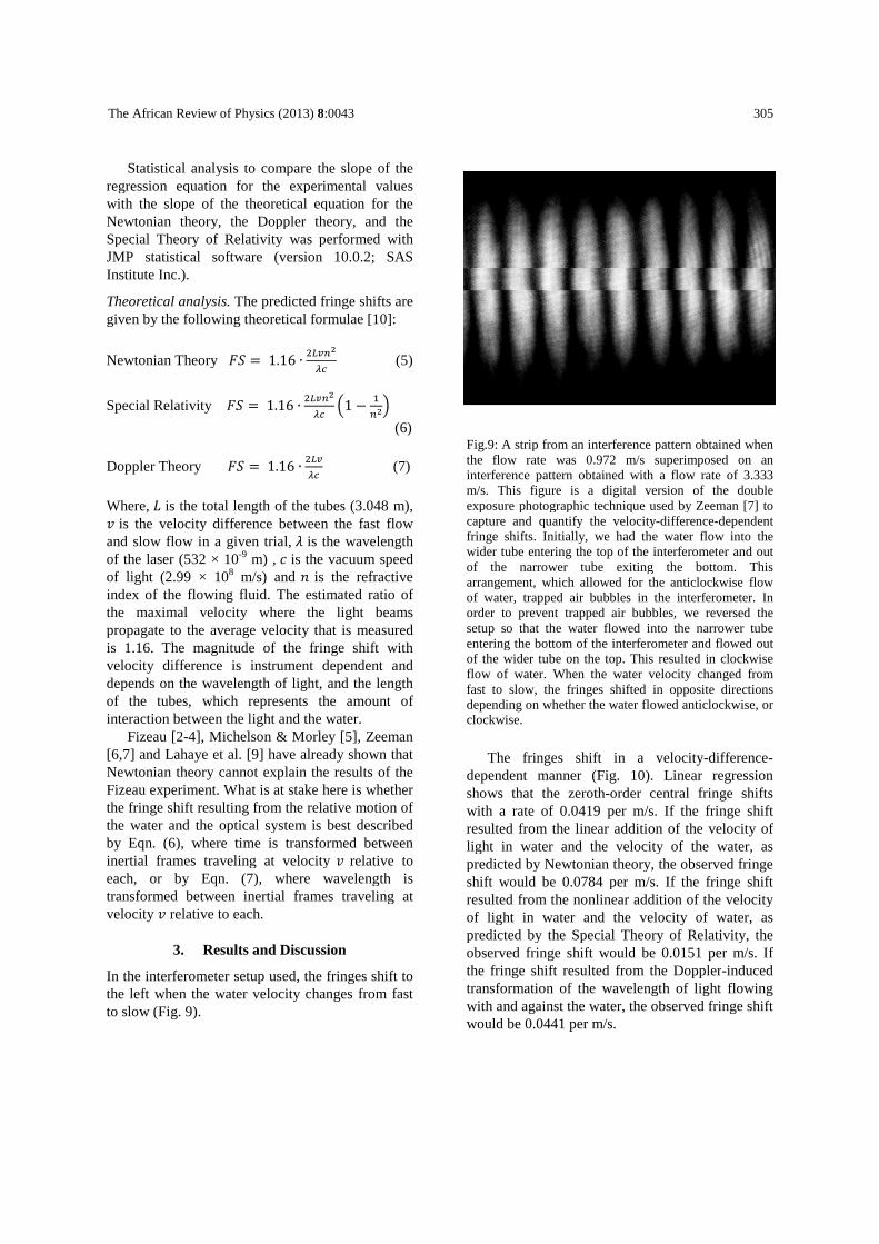
Fig.9: A strip from an interference pattern obtained the flow rate was 0.972 m/sinterference pattern obtained with a flow rate of 3.333 m/s. This figure is a digital version of the double exposure photographic technique used by Zeeman [7] to capture and quantify the velocityfringe shifts. Initially, we had the water flow into the wider tube entering the top of the interfeof the narrower tube exitingarrangement, which allowed for of water, trapped air bubbles in the interferometerorder to prevent trapped air bubblessetup so that the water flowedentering the bottom of the interferometer and flowed outof the wider tube on the top. This resulted in clockwise flow of water. When the water velocity changed from fast to slow, the fringes shifted in opposite directions depending on whether the water flowed anticlockwise.

The fringes shift in a velocitydependent manner (Fig. 10shows that the zeroth-order central with a rate of 0.0419 per m/s. If the fringe shift resulted from the linear addition of the velocity of light in water and the velocity of the water, predicted by Newtonian theory, shift would be 0.0784 per m/s. If the fringe shift resulted from the nonlinear addition of the velocity of light in water and the velocity of water, predicted by the Special Theory of Relativity, observed fringe shift would be the fringe shift resulted from the Dopplertransformation of the wavelength of light flowing with and against the water, the would be 0.0441 per m/s.

305

A strip from an interference pattern obtained when m/s superimposed on an

d with a flow rate of 3.333 This figure is a digital version of the double

exposure photographic technique used by Zeeman [7] to capture and quantify the velocity-difference-dependent

Initially, we had the water flow into the the top of the interferometer and out tube exiting the bottom. This

, which allowed for the anticlockwise flow trapped air bubbles in the interferometer. In

trapped air bubbles, we reversed the setup so that the water flowed into the narrower tube entering the bottom of the interferometer and flowed out

. This resulted in clockwise When the water velocity changed from

fast to slow, the fringes shifted in opposite directions whether the water flowed anticlockwise, or

he fringes shift in a velocity-difference-10). Linear regression

order central fringe shifts per m/s. If the fringe shift

resulted from the linear addition of the velocity of light in water and the velocity of the water, as predicted by Newtonian theory, the observed fringe

per m/s. If the fringe shift resulted from the nonlinear addition of the velocity of light in water and the velocity of water, as predicted by the Special Theory of Relativity, the

shift would be 0.0151 per m/s. If from the Doppler-induced

transformation of the wavelength of light flowing with and against the water, the observed fringe shift


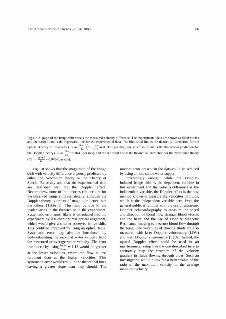
Fig.10: A graph of the fringe shift versus the and the dashed line is the regression line for the experimental data. The

Special Theory of Relativity (67 = �</�=the Doppler theory (67 = �</�= = 0.0441

(67 = �</�B

�= = 0.0784 per m/s).

Fig. 10 shows that the magnitude of the fringe

shift with velocity difference is poorly predicted by either the Newtonian theory or Special Relativity and that the experimental data are described well by the Doppler effectNevertheless, none of the theories can account for the observed fringe shift statisticallyDoppler theory is orders of magnitude better than the others (Table 1). This may be due to the inadequacies in the theories or in the experiment. Systematic error most likely is introduced into the experiment by less-than-optimal optical which would give a smaller observed fringe shift. This could be improved by using anSystematic error may also be introduced by underestimating the maximal water velocitythe measured or average water velocity. The error introduced by using

/EFG/FHI

= 1.16would be greater

at the lower velocities, where thturbulent than at the higher velocities. This systematic error would result in the theoretical lines having a greater slope than they should.

8:0043

A graph of the fringe shift versus the measured velocity difference. The experimental data are shown as filled circles and the dashed line is the regression line for the experimental data. The blue solid line is the theoretical

</�B�= C1 − �

�BD = 0.0151 per m/s), the green solid line is the

= 0.0441 per m/s), and the red solid line is the theoretical prediction for the

shows that the magnitude of the fringe is poorly predicted by

either the Newtonian theory or the Theory of he experimental data

described well by the Doppler effect. of the theories can account for

statistically, although the Doppler theory is orders of magnitude better than

. This may be due to the inadequacies in the theories or in the experiment. Systematic error most likely is introduced into the

optical alignment, which would give a smaller observed fringe shift.

sing an optical table. Systematic error may also be introduced by underestimating the maximal water velocity from the measured or average water velocity. The error

would be greater

at the lower velocities, where the flow is less turbulent than at the higher velocities. This systematic error would result in the theoretical lines having a greater slope than they should. The

random error present in the data could be reduced by using a more stable water supply.

Interestingly enough, induced fringe shift is the dependent variable this experiment and the velocityindependent variable, the Doppler effect method known to measure the velocities of fluidswhich is the independent variable heregeneral public is familiar with the use of uDoppler echocardiography and direction of blood flow through blood vessels and the heart and the use of Resonance Imaging to measure blood flow through the brain. The velocities of flomeasured with laser Doppler velocimetry (LDV) and laser Doppler anemometry (LDA). optical Doppler effect could interferometer setup like the one deaccurately map the structure of the velocity gradient in fluids flowing through pipesinvestigation would allow for a better value of the ratio of the maximum velocity to the average measured velocity.

306

velocity difference. The experimental data are shown as filled circles the theoretical prediction for the

the theoretical prediction for

red solid line is the theoretical prediction for the Newtonian theory

random error present in the data could be reduced by using a more stable water supply.

tingly enough, while the Doppler-induced fringe shift is the dependent variable in

and the velocity-difference is the Doppler effect is the best

method known to measure the velocities of fluids, ndent variable here. Even the

general public is familiar with the use of ultrasonic raphy to measure the speed

and direction of blood flow through blood vessels the use of Doppler Magnetic to measure blood flow through

The velocities of flowing fluids are also aser Doppler velocimetry (LDV)

metry (LDA). Indeed, the optical Doppler effect could be used in an interferometer setup like the one described here to

map the structure of the velocity gradient in fluids flowing through pipes. Such an investigation would allow for a better value of the ratio of the maximum velocity to the average


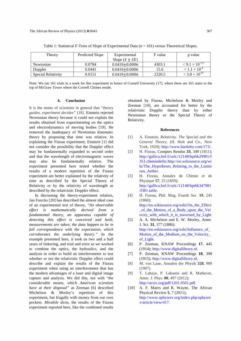
Table 1: Statistical F-Tests of Slope of Experimental Data (n = 161) versus Theoretical Slopes.

Theory Predicted Slope Experimental Slope (4̅ ± 7L)

F value p value

Newtonian 0.0784 0.0419±0.0006 4303.1 < 9.1 × 10-117 Doppler 0.0441 0.0419±0.0006 15.6 < 1.1 × 10-4 Special Relativity 0.0151 0.0419±0.0006 2320.5 < 3.8 × 10-97

Note: We ran 161 trials in a week for this experiment in honor of Cornell University [17], where there are 161 stairs to the top of McGraw Tower where the Cornell Chimes reside.

4. Conclusion

It is the motto of scientists in general that “theory guides, experiment decides” [18]. Einstein rejected Newtonian theory because it could not explain the results obtained from experimenting on the optics and electrodynamics of moving bodies [19]. He removed the inadequacy of Newtonian kinematic theory by proposing that time was relative. In explaining the Fizeau experiment, Einstein [1] did not consider the possibility that the Doppler effect may be fundamentally expanded to second order and that the wavelength of electromagnetic waves may also be fundamentally relative. The experiment presented here tested whether the results of a modern repetition of the Fizeau experiment are better explained by the relativity of time as described by the Special Theory of Relativity or by the relativity of wavelength as described by the relativistic Doppler effect.

In discussing the theory-experiment relation, Jan Frercks [20] has described the almost ideal case of an experimental test of theory, “An observable effect is mathematically derived from a fundamental theory, an apparatus capable of detecting this effect is conceived and built, measurements are taken, the data happen to be in full correspondence with the expectation, which corroborates the underlying theory.” In the example presented here, it took us two and a half years of tinkering, and trial and error as we worked to combine the optics, the hydraulics, and the analysis in order to build an interferometer to test whether or not the relativistic Doppler effect could describe and explain the results of the Fizeau experiment when using an interferometer that has the modern advantages of a laser and digital image capture and analysis. We did this, not with “the considerable means, which American scientists have at their disposal” as Zeeman [6] described Michelson & Morley’s repetition of this experiment, but frugally with money from our own pockets. Mirabile dictu, the results of the Fizeau experiment reported here, like the combined results

obtained by Fizeau, Michelson & Morley and Zeeman [10], are accounted for better by the relativistic Doppler theory than by either Newtonian theory or the Special Theory of Relativity.

References

[1] A. Einstein, Relativity. The Special and the General Theory, (H. Holt and Co., New York, 1920); http://www.bartleby.com/173/.

[2] H. Fizeau, Comptes Rendus 33, 349 (1851); http://gallica.bnf.fr/ark:/12148/bpt6k29901/f351.chemindefer.http://en.wikisource.org/wiki/The_Hypotheses_Relating_to_the_Luminous_Aether.

[3] H. Fizeau, Annales de Chimie et de Physique 57, 25 (1859); http://gallica.bnf.fr/ark:/12148/bpt6k347981/f381.table.

[4] H. Fizeau, Phil. Mag. Fourth Ser. 19, 245 (1860); http://en.wikisource.org/wiki/On_the_Effect_of_the_Motion_of_a_Body_upon_the_Velocity_with_which_it_is_traversed_by_Light

[5] A. A. Michelson and E. W. Morley, Amer. J. Sci. 31, 377 (1886); http://en.wikisource.org/wiki/Influence_of_Motion_of_the_Medium_on_the_Velocity_of_Light.

[6] P. Zeeman, KNAW Proceedings 17, 445 (1914); http://www.digitallibrary.nl.

[7] P. Zeeman, KNAW Proceedings 18, 398 (1915); http://www.digitallibrary.nl.

[8] M. von Laue, Annalen der Physik 328, 989 (1907).

[9] T. Lahaye, P. Labastie and R. Mathevet, Amer. J. Phys. 80, 497 (2012); http://arxiv.org/pdf/1201.0501.pdf.

[10] A. F. Maers and R. Wayne, The African Physical Review 5, 7 (2011); http://www.aphysrev.org/index.php/aphysrev/article/view/417.


[11] R. Wayne, The African Physical Review 4, 43 (2010); http://www.aphysrev.org/index.php/aphysrev/article/view/369/175.

[12] R. Wayne, The African Review of Physics 7, 115 (2012); http://www.aphysrev.org/index.php/aphysrev/article/view/539/233.

[13] R. Wayne, Acta Physica Polonica B 41, 2297 (2010); http://www.aphysrev.org/index.php/aphysrev/article/view/369/175.

[14] G. Weinstein, “Albert Einstein and the Fizeau 1851 water tube experiment”; http://arxiv.org/abs/1204.3390 (2012).

[15] K. J. Niklas and H.-C. Spatz, Plant Physics (University of Chicago Press, Chicago, 2012).

[16] N. Bowditch, Memoirs of the American Academy of Arts and Sciences 3, 413 (1809).

[17] Cornell Alumni Magazine 97, 36 (1995); http://ecommons.library.cornell.edu/handle/1813/28109.

[18] I. M. Kolthoff, Volumetric Analysis (J. Wiley & Sons, New York, 1928).

[19] F. S. C. Northrop, Science and First Principles (Macmillan Co., New York, 1931).

[20] J. Frercks, Boston Studies in the Philosophy of Science 267,179 (2009).

Appendix: MATLAB program for analyzing the data

Program: fizeau % Analysis of fringe displacement in a Fizeau inter ferometer % Set Shift Direction % If the observed fringe shift is from the right to the left when the % velocity of the water is decreased, set the follo wing variable to 1, % otherwise if the observed fringe shift is from th e left to the right when % the velocity of the water is decreased, set the f ollowing variable to 0. left=1; % Set Number of Imgs % Set 'start' number to at least 101 and set 'numim g' to 101 plus the % number of trials to be analyzed. start=101; numimg=110; % Initialize the Output Matrix output = { 'Fringe #' ;1;2;3;4;5;6;7;8;9;10;11;12;13;14;15;16;17;18;19;20 }; output{24,1}= 'Voltage-Velocity Factor' ; output{24,2}=0.7714624195; output{25,1}= 'Fast Velocity' ; output{26,1}= 'Slow Velocity' ; output{27,1}= 'Change in Velocity' ; output{29,1}= 'Water Factor' ; output{29,2}=1.16; output{30,1}= 'Special Relativity' ; output{30,2}=0.013; output{31,1}= 'Doppler Effect' ; output{31,2}=0.038; % Read in the Imgs for i=start:numimg eval([ 's' num2str(i) '=imread(''slow' num2str(i) '.TIF'');' ]); eval([ 'f' num2str(i) '=imread(''fast' num2str(i) '.TIF'');' ]); end


% Analyze the Imgs for j=start:numimg eval([ 'output{1,j-99}=' '''Trial ' num2str(j-100) ''';' ]); eval([ '[output] = imageanalysis(s' num2str(j) ', f' num2str(j) ', j, output, left);' ]); end % Export the output matrix to excel xlswrite( 'output.xlsx' , output); Function: imageanalysis function [output] = imageanalysis(s1, f1, j, output, left) % Creates output figures using manual cropping close all % Crop the images [s2, rect]=imcrop(s1); close all f2=imcrop(f1, rect); % Calculate means smean=mean(s2); fmean=mean(f2); % Smooth means smean=smooth(smean, 5); fmean=smooth(fmean, 5); % Find troughs using peakfinder sindex = peakfinder(smean, 50, 175, -1); findex = peakfinder(fmean, 50, 175, -1); % Segment the cropped images into individual fringe s slength = length(sindex); flength = length(findex); numfringes = slength-1; if slength == flength for i=1:numfringes if left == 1 width = sindex(i+1)-findex(i); fringei = [findex(i) rect(2) width rect (4)]; else width = findex(i+1)-sindex(i); fringei = [sindex(i) rect(2) width rect (4)]; end eval([ 's' num2str(i+2) '=imcrop(s1, fringei);' ]); eval([ 'f' num2str(i+2) '=imcrop(f1, fringei);' ]); % Calculate means eval([ 'smean' num2str(i+2) '=mean(s' num2str(i+2) ');' ]);


eval([ 'fmean' num2str(i+2) '=mean(f' num2str(i+2) ');' ]); % Smooth means eval([ 'smean' num2str(i+2) '=smooth(smean' num2str(i+2) ', 5);' ]); eval([ 'fmean' num2str(i+2) '=smooth(fmean' num2str(i+2) ', 5);' ]); end else error( 'slength= %g flength= %g' , slength, flength); end % Plot Slow and Fast Means subplot(3,1,3), plot(smean); axis([0 872 0 255]); set(gca, 'XTick' ,0:109:872); set(gca, 'YTick' ,0:51:255); xlabel( 'Pixel' ); ylabel( 'Intensity' ); str=sprintf( 'Slow = Blue Fast = Green' ); title(str); hold all subplot(3,1,3), plot(fmean); % Plot Cropped Images subplot(3,1,1), subimage(s2); set(gca, 'XTick' ,0:109:872); set(gca, 'YTick' ,[]); title( 'Slow' ); xlabel( 'Pixel' ); subplot(3,1,2), subimage(f2); set(gca, 'XTick' ,0:109:872); set(gca, 'YTick' ,[]); title( 'Fast' ); xlabel( 'Pixel' ); eval([ 'save2word(''output' num2str(j) '.doc'')' ]); close all % Plot Segmented Fringes figure for i=1:numfringes eval([ 'subplot(2,numfringes,i), subimage(s' num2str(i+2) ');' ]); set(gca, 'XTick' ,[]); set(gca, 'YTick' ,[]); eval([ 'subplot(2,numfringes,i+numfringes), subimage(f' num2str(i+2) ');' ]); set(gca, 'XTick' ,[]); set(gca, 'YTick' ,[]); end % Title the Segmented Fringes annotation( 'textbox' , [0 0.9 1 0.06], 'string' , 'Slow Fringes' , 'HorizontalAlignment' , 'center' ); annotation( 'textbox' , [0 0.45 1 0.06], 'string' , 'Fast Fringes' , 'HorizontalAlignment' , 'center' ); eval([ 'save2word(''output' num2str(j) '.doc'')' ]);


close all % Plot the Lissajous Figures for i=1:numfringes % Fit an ellipse eval([ '[semimajor_axis' num2str(i+2) ', semiminor_axis' num2str(i+2) ', x0' num2str(i+2) ', y0' num2str(i+2) ', phi' num2str(i+2) '] = ellipse_fit(smean' num2str(i+2) ', fmean' num2str(i+2) ');' ]); % Calculate fringe shift eval([ 'fs' num2str(i+2) ' = (semiminor_axis' num2str(i+2) '/ semimajor_axis' num2str(i+2) ')/4;' ]); % Plot Lissajous figure figure eval([ 'plot(smean' num2str(i+2) ', fmean' num2str(i+2) ');' ]); axis([0 255 0 255]); set(gca, 'XTick' ,0:51:255); set(gca, 'YTick' ,0:51:255); xlabel( 'Slow Intensity' ); ylabel( 'Fast Intensity' ); str=sprintf( 'Fringe %i Experimental Data = Blue Fitted Ellipse = Red' , i); title(str); hold all % Plot fitted ellipse color = 'r' ; eval([ 'ellipse(semimajor_axis' num2str(i+2) ', semiminor_axis' num2str(i+2) ', phi' num2str(i+2) ', x0' num2str(i+2) ', y0' num2str(i+2) ', color);' ]); eval([ 'save2word(''output' num2str(j) '.doc'')' ]); close all end % Add calculated shifts to output matrix for i=1:numfringes eval([ 'output{i+1,j-99}=fs' num2str(i+2) ';' ]); end end

The following functions used in the above analysis programs were written by others and downloaded from

www.mathworks.com.

Function: Peakfinder http://www.mathworks.com/matlabcentral/fileexchange/25500-peakfinder/content/peakfinder.m

Copyright Nathanael C. Yoder 2011 [email protected].


Function: Ellipse http://www.mathworks.com/matlabcentral/fileexchange/289-ellipse-m/content/ellipse.m Written by D.G. Long, Brigham Young University, based on the CIRCLES.m original written by Peter Blattner, Institute of Microtechnology, University of Neuchatel, Switzerland, [email protected] Function: Ellipse_fit http://www.mathworks.com/matlabcentral/fileexchange/22423-ellipse-fit/content/ellipse_fit.m Programmed by: Tal Hendel [email protected] Faculty of Biomedical Engineering, Technion- Israel Institute of Technology, Dec-2008 Function: Save2Word http://www.mathworks.com/matlabcentral/fileexchange/3149-save2word/content/save2word.m Suresh E Joel, Mar 6, 2003, Virginia Commonwealth University, Modification of 'saveppt' in Mathworks File Exchange and valuable suggestions by Mark W. Brown, [email protected].

Received: 28 May, 2013 Accepted: 6 September, 2013

The Fizeau Experiment: Experimental Investigations of the...

Documents

Transcript of The Fizeau Experiment: Experimental Investigations of the...